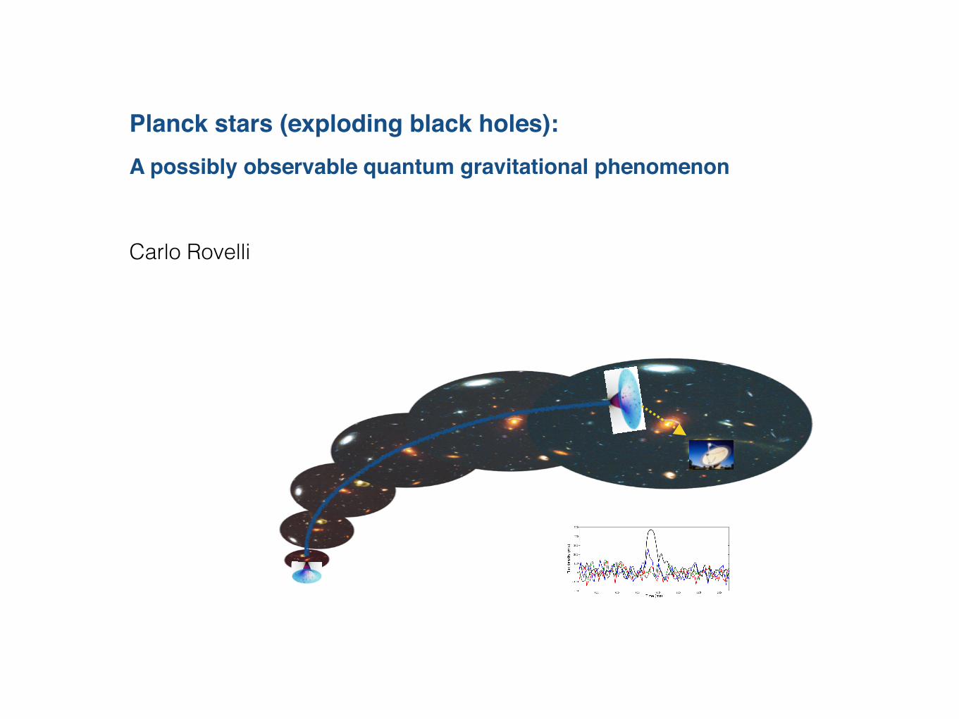
Planck stars (exploding black holes): A possibly observable quantum gravitational phenomenon

Carlo Rovelli

A real-time FRB 5

Figure 2. The full-Stokes parameters of FRB 140514 recorded in the centre beam of the multibeam receiver with BPSR. Total intensity,and Stokes Q, U , and V are represented in black, red, green, and blue, respectively. FRB 140514 has 21 ± 7% (3-�) circular polarisationaveraged over the pulse, and a 1-� upper limit on linear polarisation of L < 10%. On the leading edge of the pulse the circular polarisationis 42 ± 9% (5-�) of the total intensity. The data have been smoothed from an initial sampling of 64 µs using a Gaussian filter of full-widthhalf-maximum 90 µs.

source given the temporal proximity of the GMRT observa-tion and the FRB detection. The other two sources, GMRT2and GMRT3, correlated well with positions for known ra-dio sources in the NVSS catalog with consistent flux densi-ties. Subsequent observations were taken through the GMRTToO queue on 20 May, 3 June, and 8 June in the 325 MHz,1390 MHz, and 610 MHz bands, respectively. The secondepoch was largely unusable due to technical di�culties. Thesearch for variablility focused on monitoring each source forflux variations across observing epochs. All sources from thefirst epoch appeared in the third and fourth epochs with nomeasureable change in flux densities.

4.4 Swift X-Ray Telescope

The first observation of the FRB 140514 field was taken us-ing Swift XRT (Gehrels et al. 2004) only 8.5 hours after theFRB was discovered at Parkes. This was the fastest Swiftfollow-up ever undertaken for an FRB. 4 ks of XRT datawere taken in the first epoch, and a further 2 ks of datawere taken in a second epoch later that day, 23 hours af-ter FRB 140514, to search for short term variability. A finalepoch, 18 days later, was taken to search for long term vari-ability. Two X-ray sources were identified in the first epochof data within the 150 diameter of the Parkes beam. Bothsources were consistent with sources in the USNO catalog(Monet et al. 2003). The first source (XRT1) is located atRA = 22:34:41.49, Dec = -12:21:39.8 with RUSNO = 17.5and the second (XRT2) is located at RA = 22:34:02.33 Dec= -12:08:48.2 with RUSNO = 19.7. Both XRT1 and XRT2appeared in all subsequent epochs with no observable vari-ability on the level of 10% and 20% for XRT1 and XRT2,respectively, both calculated from photon counts from theXRT. Both sources were later found to be active galacticnuclei (AGN).

4.5 Gamma-Ray Burst Optical/Near-InfraredDetector

After 13 hours, a trigger was sent to the Gamma-Ray BurstOptical/Near-Infrared Detector (GROND) operating on the2.2-m MPI/ESO telescope on La Silla in Chile (Greiner et al.2008). GROND is able to observe simultaneously in J , H,and K near-infrared (NIR) bands with a 100 ⇥ 100 field ofview (FOV) and the optical g0, r0, i0, and z0 bands with a60 ⇥ 60 FOV. A 2⇥2 tiling observation was done, providing61% (JHK) and 22% (g0r0i0z0) coverage of the inner partof the FRB error circle. The first epoch began 16 hours af-ter FRB 140514 with 460 second exposures, and a secondepoch was taken 2.5 days after the FRB with an identicalobserving setup and 690 s (g0r0i0z0) and 720 s (JHK) ex-posures, respectively. Limiting magnitudes for J , H, and Kbands were 21.1, 20.4, and 18.4 in the first epoch and 21.1,20.5, and 18.6 in the second epoch, respectively (all in theAB system). Of all the objects in the field, analysis iden-tified three variable objects, all very close to the limitingmagnitude and varying on scales of 0.2 - 0.8 mag in the NIRbands identified with di↵erence imaging. Of the three ob-jects one is a galaxy, another is likely to be an AGN, andthe last is a main sequence star. Both XRT1 and GMRT1sources were also detected in the GROND infrared imagingbut were not observed to vary in the infrared bands on thetimescales probed.

4.6 Swope Telescope

An optical image of the FRB field was taken 16h51m afterthe burst event with the 1-m Swope Telescope at Las Cam-panas. The field was re-imaged with the Swope Telescope on17 May, 2 days after the FRB. No variable optical sources

c� 0000 RAS, MNRAS 000, 000–000

Planck stars (exploding black holes): A possibly observable quantum gravitational phenomenon

Carlo Rovelli

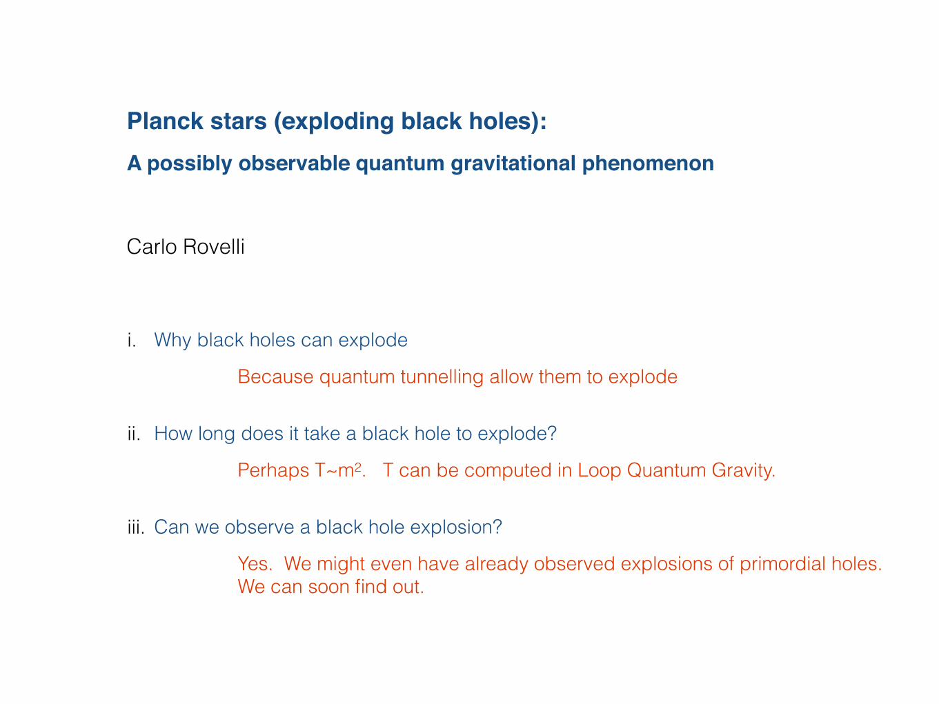
i. Why black holes can explode

ii. How long does it take a black hole to explode?

iii. Can we observe a black hole explosion?

Because quantum tunnelling allow them to explode

Perhaps T~m2. T can be computed in Loop Quantum Gravity.

Yes. We might even have already observed explosions of primordial holes.We can soon find out.

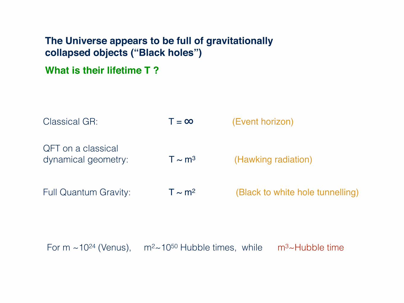
The Universe appears to be full of gravitationally collapsed objects (“Black holes”)What is their lifetime T ?

Classical GR: T = ∞ (Event horizon)

QFT on a classical dynamical geometry: T ~ m3 (Hawking radiation)

Full Quantum Gravity: T ~ m2 (Black to white hole tunnelling)

For m ~1024 (Venus), m2~1050 Hubble times, while m3~Hubble time

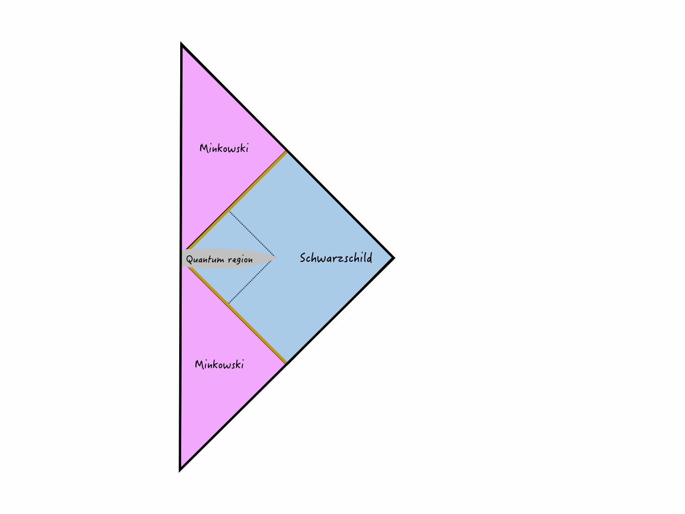
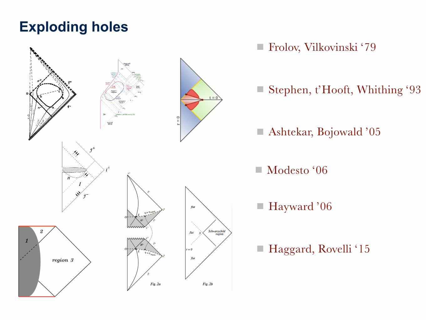
A clear theme emerges from these spacetime diagrams:⌥ build a time symmetric model

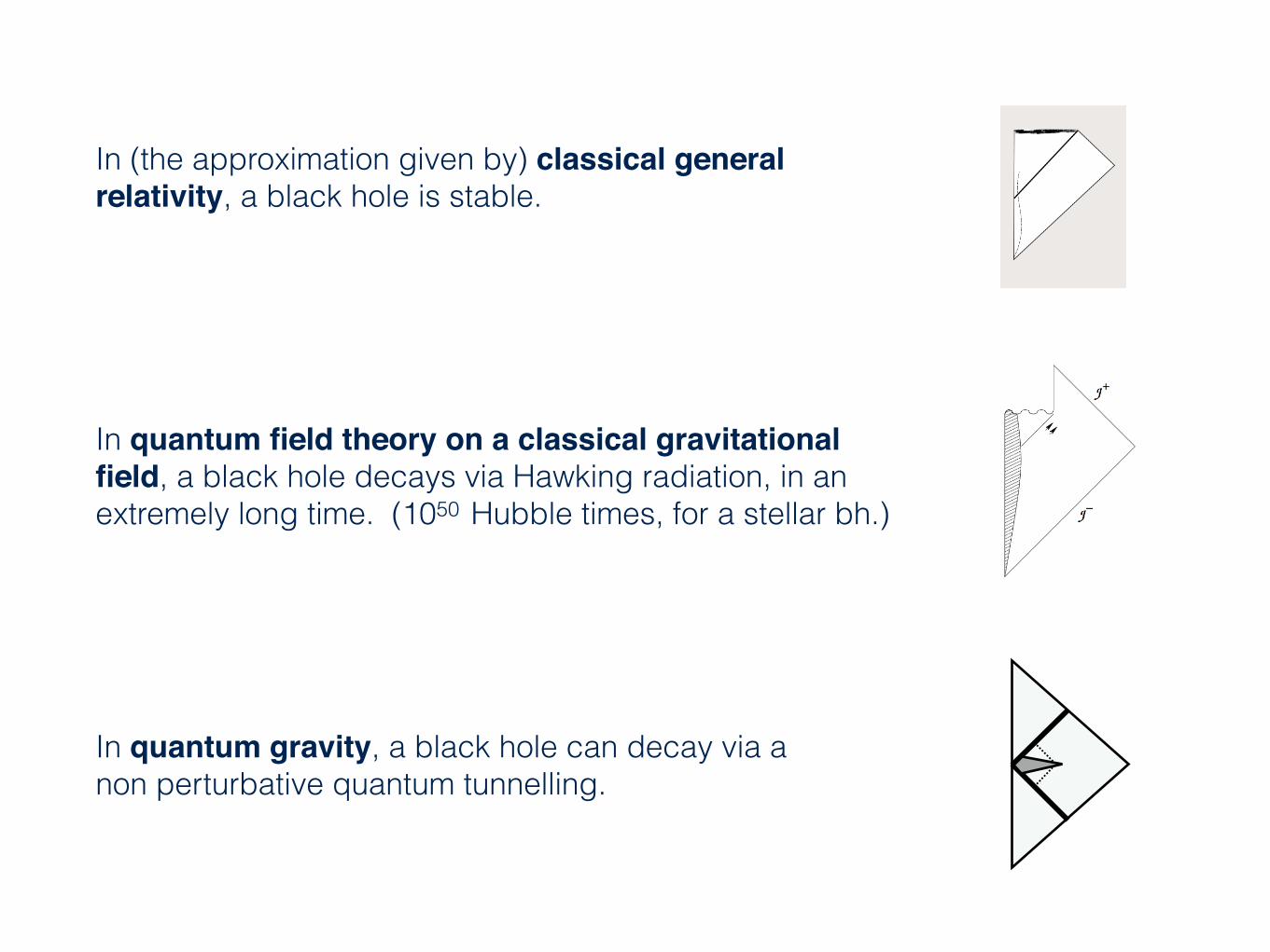
In (the approximation given by) classical general relativity, a black hole is stable.

Two deep puzzles we have all wondered about:

A brief (very incomplete) history of ideas

In quantum field theory on a classical gravitational field, a black hole decays via Hawking radiation, in an extremely long time. (1050 Hubble times, for a stellar bh.)

In quantum gravity, a black hole can decay via a non perturbative quantum tunnelling.

I

I I

I

What happens here?

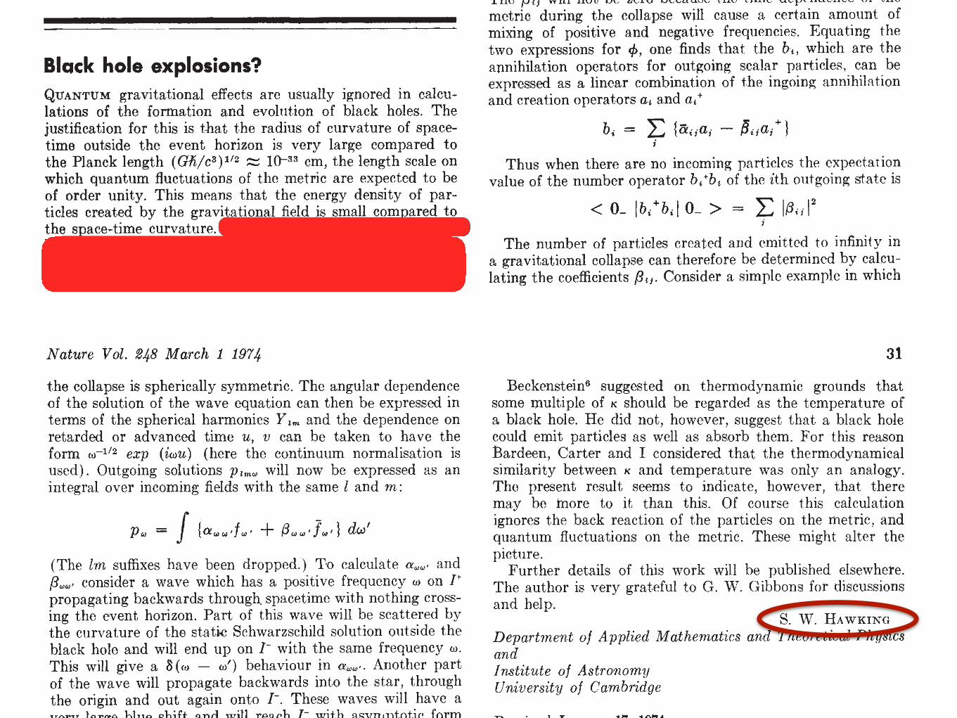
© 1974 Nature Publishing Group

© 1974 Nature Publishing Group

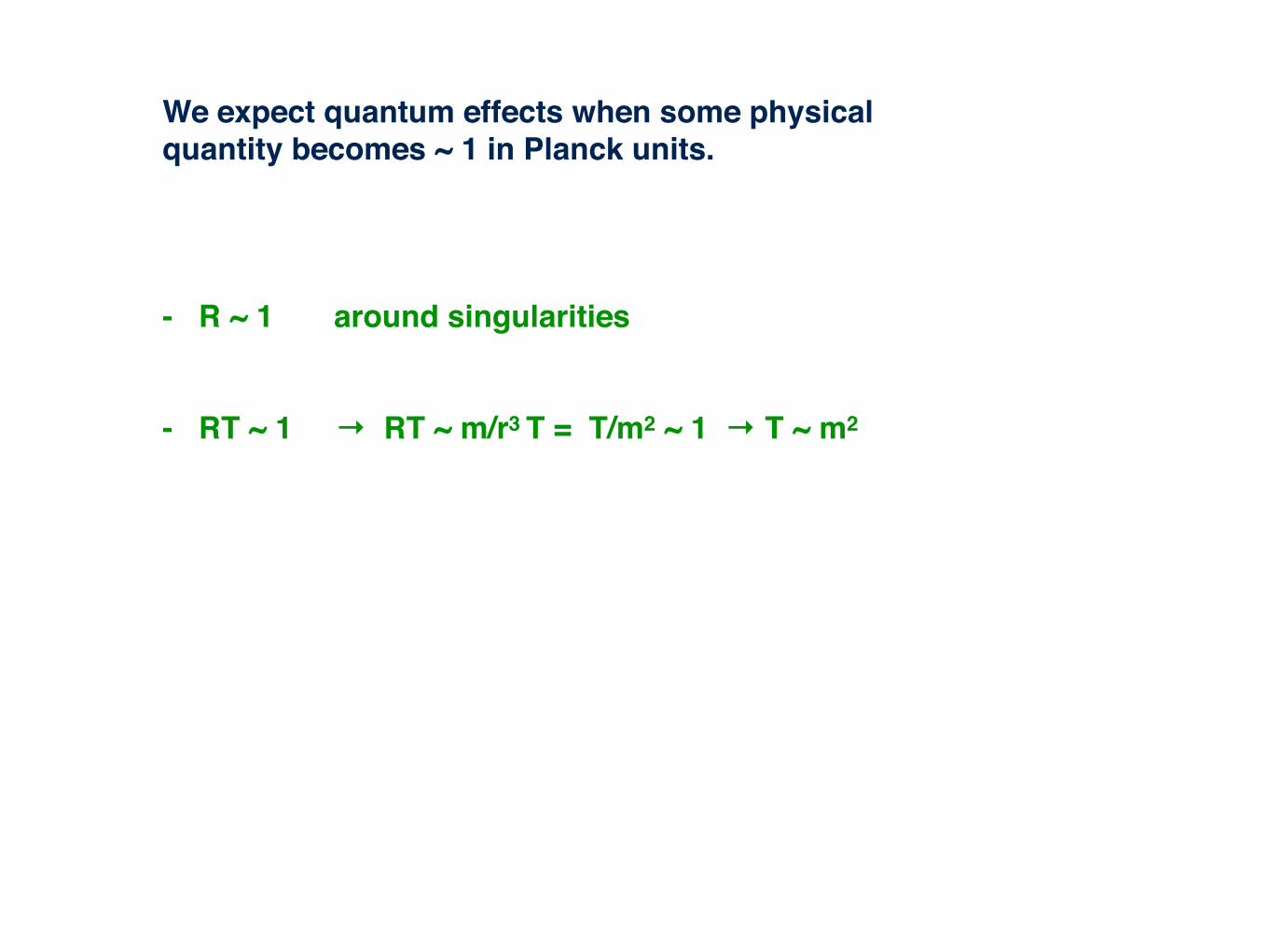
We expect quantum effects when some physical quantity becomes ~ 1 in Planck units.

- R ~ 1 around singularities

- RT ~ 1 → RT ~ m/r3 T = T/m2 ~ 1 → T ~ m2

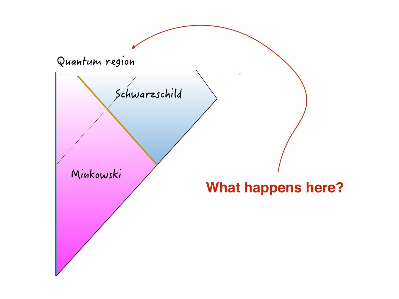
What happens here?

In ’05

Abhay Ashtekar

Martin Bojowald

At MG2 and in a paper ’79-’81

Valeri Frolov

Grigori A. Vilkovisky (left)

In ’93

Cristopher R. Stephens

Gerard ’t Hooft

Bernard F. Whiting

Exploding holesFrolov, Vilkovinski ‘79

Stephen, t’Hooft, Whithing ‘93

Ashtekar, Bojowald ’05

Hayward ’06

Haggard, Rovelli ‘15

Modesto ‘06

region 3

2

1

Figure 2: Penrose diagram for the gravitational collapse inside the event horizon (Region 1 and region2) and outside the event horizon (Region3).

Solving the constraints equations (9) we obtain the known results for the classical dust matter gravi-tational collapse [8].

2 Gravitational collapse in Ashtekar variables

In this section we study the gravitational collapse in Ashtekar variables [12]. In particular we willexpress the Hamiltonian constraint inside and outside the matter and the constraints P1 and P2 interms of the symmetric reduced Ashtekar connection [13], [14].

2.1 Ashtekar variables

In LQG the fundamental variables are the Ashtekar variables: they consist of an SU(2) connectionAi

a and the electric field Eai , where a, b, c, · · · = 1, 2, 3 are tensorial indices on the spatial section and

i, j, k, · · · = 1, 2, 3 are indices in the su(2) algebra. The density weighted triad Eai is related to the

triad eia by the relation Ea

i = 12ϵ

abc ϵijk ejb ek

c . The metric is related to the triad by qab = eia ej

b δij .Equivalently,

!

det(q) qab = Eai Eb

j δij . (10)

The rest of the relation between the variables (Aia, Ea

i ) and the ADM variables (qab, Kab) is given by

Aia = Γi

a + γKabEbjδ

ij (11)

where γ is the Immirzi parameter and Γia is the spin connection of the triad, namely the solution of

Cartan’s equation: ∂[aeib] + ϵijk Γj

[aekb] = 0.

The action is

S =1

κ γ

"

dt

"

Σd3x

#

−2Tr(EaAa) − NH− NaHa − N iGi

$

, (12)

where Na is the shift vector, N is the lapse function and N i is the Lagrange multiplier for the Gaussconstraint Gi. We have introduced also the notation E[1] = Ea∂a = Ea

i τi∂a and A[1] = Aadxa =

Aiaτ

idxa. The functions H, Ha and Gi are respectively the Hamiltonian, diffeomorphism and Gauss

4

Sean A. Hayward in ’06

[see M. Smerlak’s talk]

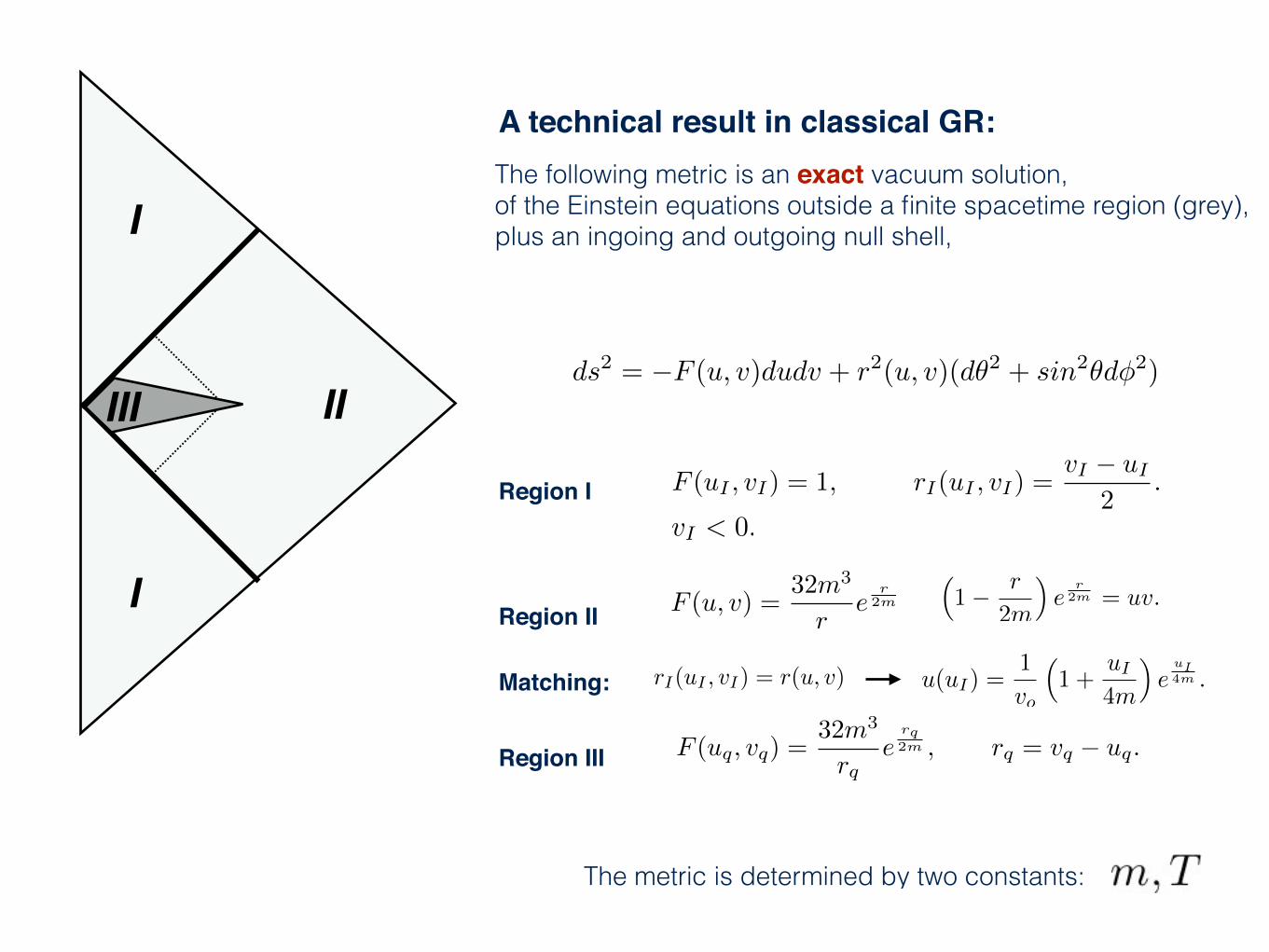
A technical result in classical GR:The following metric is an exact vacuum solution, of the Einstein equations outside a finite spacetime region (grey), plus an ingoing and outgoing null shell,

ds2 = �F (u, v)dudv + r2(u, v)(d✓2 + sin2✓d�2)

F (uI , vI) = 1, rI(uI , vI) =vI � uI

2.Region I

vI < 0.

Region II F (u, v) =32m3

re

r2m

⇣1� r

2m

⌘e

r2m = uv.

rI(uI , vI) = r(u, v)Matching: u(uI

) =1

vo

⇣1 +

uI

4m

⌘e

uI4m .

F (uq, vq) =32m3

rqe

rq2m , rq = vq � uq.Region III

The metric is determined by two constants:

I

III II

I

I

I

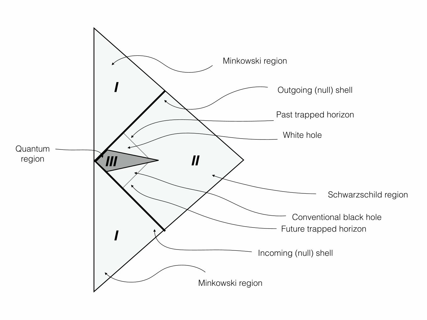
Minkowski region

Schwarzschild region

Incoming (null) shell

Outgoing (null) shell

Future trapped horizonConventional black hole

Past trapped horizon

White hole

Minkowski region

IIIIIQuantum

region

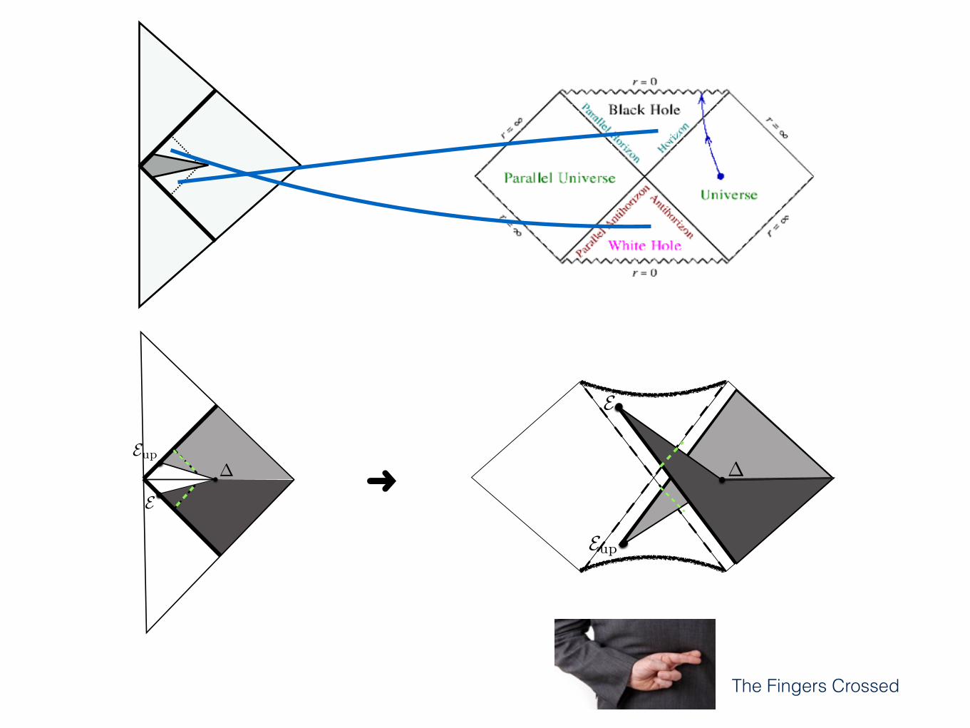
The Fingers Crossed

➜

I

I

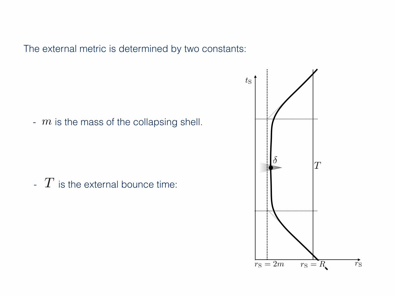
The external metric is determined by two constants:

- is the mass of the collapsing shell.m

- is the external bounce time:

r=0

r=

ar=R

t = 0τ

u

v

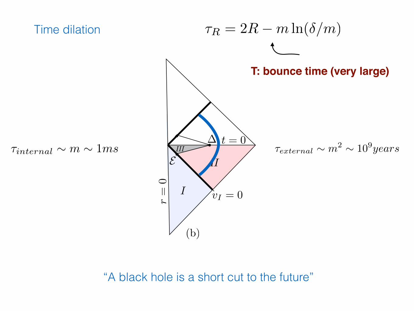
⌧internal ⇠ m ⇠ 1ms ⌧external

⇠ m2 ⇠ 109years

“A black hole is a short cut to the future”

Time dilation

T: bounce time (very large)

⌧R = 2R�m ln(�/m)

What determines T ?

Quantum gravity

�

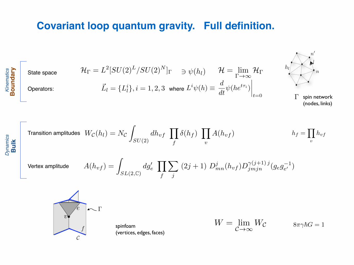
hf =Y

v

hvfTransition amplitudes

Vertex amplitude

State space

Operators: where

l

n

n0

Kinematics

Dynam

ics

�

8⇡�~G = 1

H� = L2[SU(2)L/SU(2)N ]�

WC(hl) = NC

Z

SU(2)dhvf

Y

f

�(hf )Y

v

A(hvf )

spinfoam(vertices, edges, faces)

C

f

ev

hl3 (hl)

A(hvf ) =

Z

SL(2,C)dg0e

Y

f

X

j

(2j + 1) Djmn(hvf )D

�(j+1) jjmjn (geg

�1e0 )

spin network(nodes, links)

Bou

ndar

yB

ulk

H = lim�!1

H�

W = limC!1

WC

Covariant loop quantum gravity. Full definition.

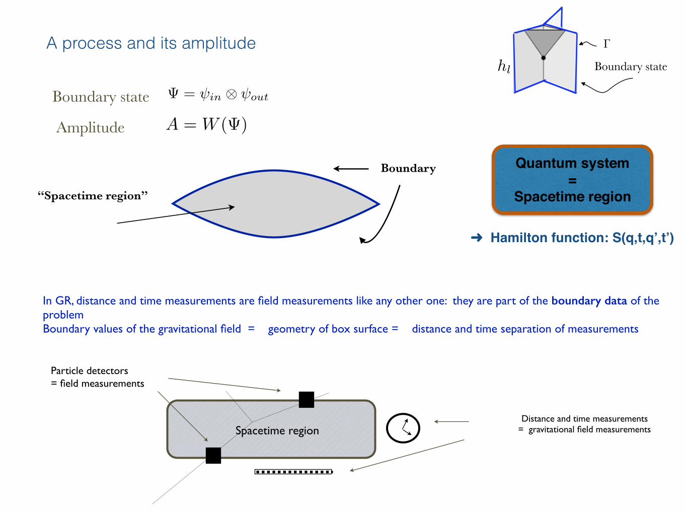
In GR, distance and time measurements are field measurements like any other one: they are part of the boundary data of the problem Boundary values of the gravitational field = geometry of box surface = distance and time separation of measurements

Spacetime region

Particle detectors = field measurements

Distance and time measurements= gravitational field measurements

“Spacetime region”

Boundary

A = W ( )

Boundary state

Amplitude

= in

⌦ out

A process and its amplitude �

hl Boundary state

Quantum system=

Spacetime region

➜ Hamilton function: S(q,t,q’,t’)

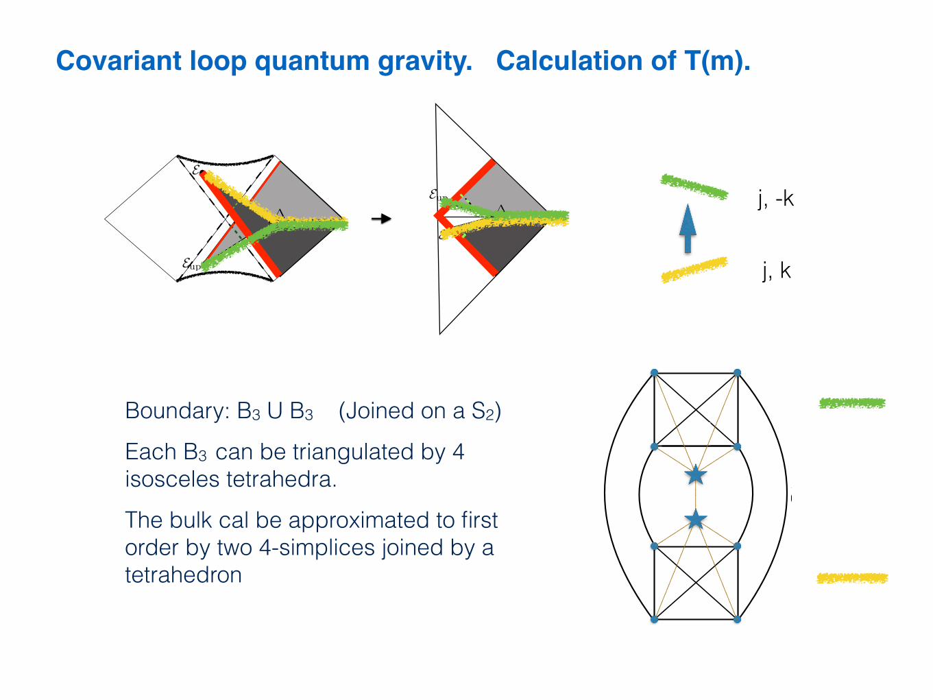
Covariant loop quantum gravity. Calculation of T(m).

j, k

j, -k

Boundary: B3 U B3 (Joined on a S2)

Each B3 can be triangulated by 4 isosceles tetrahedra.

The bulk cal be approximated to first order by two 4-simplices joined by a tetrahedron

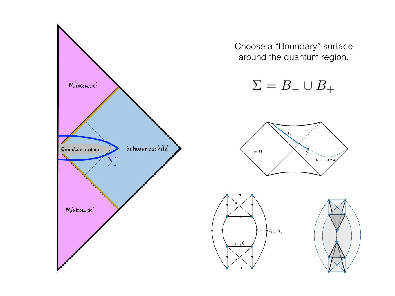
Choose a “Boundary” surface around the quantum region.

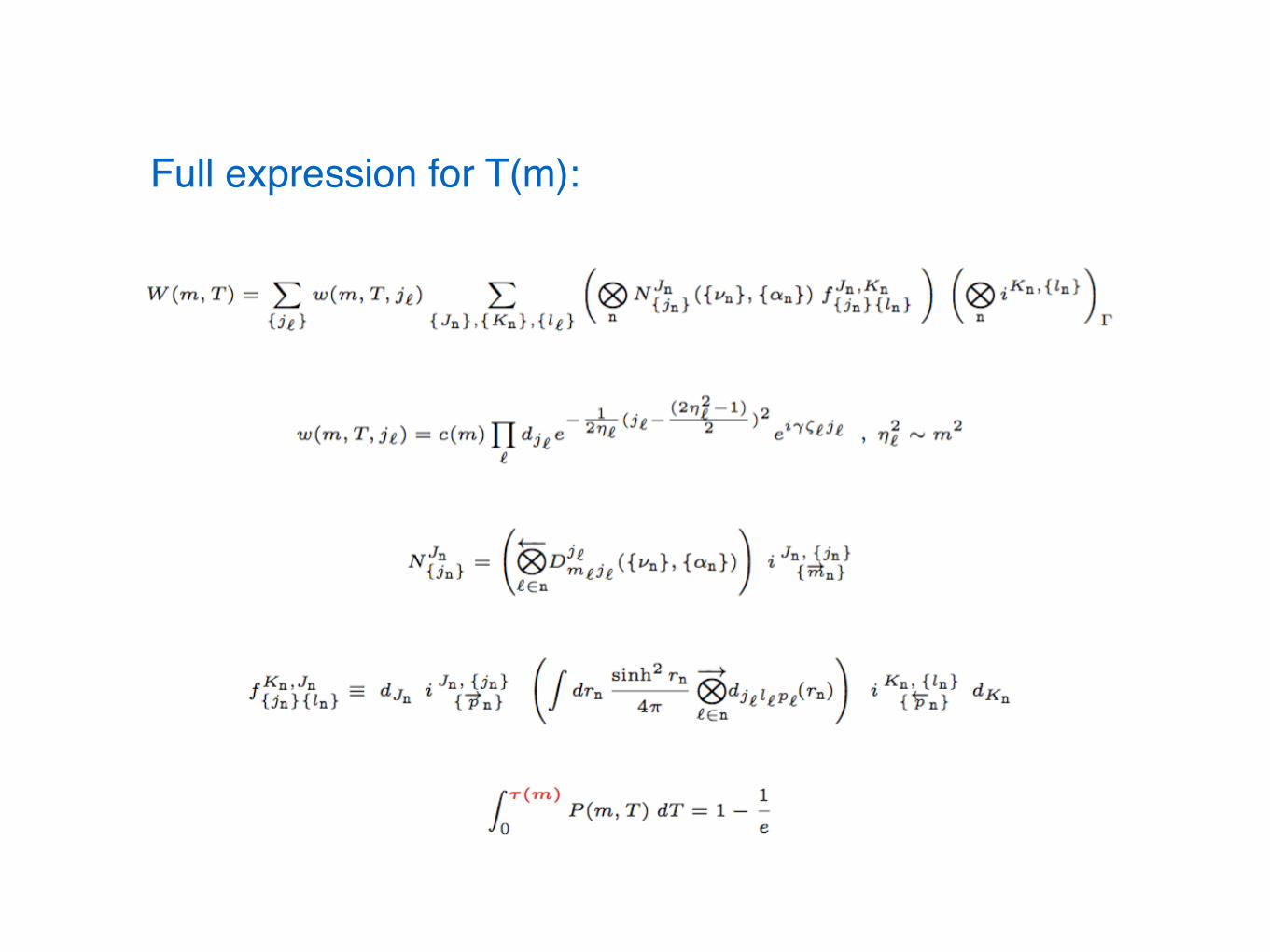
Full expression for T(m):

T ⇠ m2

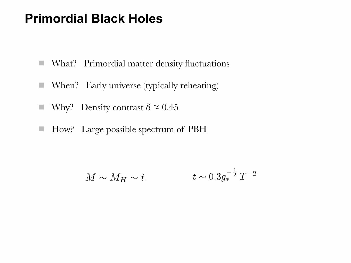
Primordial Black Holes

What? Primordial matter density fluctuations

When? Early universe (typically reheating)

Why? Density contrast δ ≈ 0.45

How? Large possible spectrum of PBH

maximal extension of the Schwarzschild metric for amass M . Region (III) is where quantum gravity becomesnon-negligible.

Importantly, by gluing together the di↵erent part ofthe e↵ective metric and estimating the time needed forquantum e↵ects to happen, it was shown that the dura-tion of the bounce should not be shorter than [10]

⌧ = 4kM2, (1)

with k > 0.05 a dimensionless parameter. We usePlanck units where G = ~ = c = 1. The bouncetime is proportional to M2 and not to M3 as in theHawking process. As long as k remains small enough,the bounce time is much smaller than the Hawkingevaporation time and the evaporation can be consideredas a dissipative correction that can be neglected in afirst order approximation.

The phenomenology was investigated in [11] under theassumption that k takes its smallest possible value, whichmakes the bounce time as short as possible. The aimof the present article is to go beyond this first study intwo directions. First, we generalize the previous resultsby varying k. The only condition for the model to bevalid is that the bounce time remains (much) smallerthan the Hawking time. This assumption is supportedby the “firewall argument” presented in [1]. We study indetail the maximal distance at which a single black-holebounce can be detected. Second, we go beyond this “sin-gle event detection” and consider the di↵use backgroundproduced by a distribution of bouncing black holes.

II. SINGLE EVENT DETECTION

For detection purposes, we are interested in blackholes whose lifetime is less than the age of the Universe.For a primordial black hole detected today, ⌧ = tHwhere tH is the Hubble time. This fixes the mass M , asa function of the parameter k (defined in the previoussection) for black holes that can be observed. In allcases considered, M is very small compared to a solarmass and therefore only primordial black holes possiblyformed in the early Universe are interesting from thispoint of view. Although no primordial black hole hasbeen detected to date, various mechanism for their pro-duction shortly after the Big Bang have been suggested(see, e.g., [12] for an early detailed calculation and [13]for a review). Although their number density might beway too small for direct detection, the production ofprimordial black holes remains a quite generic predictionof cosmological physics either directly from densityperturbations –possibly enhanced by phase transitions–or through exotic phenomena like collisions of cosmicstrings or bubbles of false vacua.

The energy (and amplitude) of the signal emitted inthe quantum gravity model considered here remainsopen. As suggested in [11] and to remain general,we consider two possible signals of di↵erent origins.The first one, referred to as the low energy signal,is determined by dimensional arguments. When thebounce is completed, the black hole (more precisely theemerging white hole) has a size (L ⇠ 2M) determined byits mass M . This is the main scale of the problem and itfixes an expected wavelength for the emitted radiation:� ⇠ L. We assume that particles are emitted at theprorata of their number of internal degrees of freedom.(This is also the case for the Hawking spectrum at theoptical limit, i.e. when the greybody factors describ-ing the backscattering probability are spin-independent.)

The second signal, referred to as the high energy com-ponent, has a very di↵erent origin. Consider the historyof the matter emerging from a white hole: it comes fromthe bounce of the matter that formed the black hole bycollapsing. In most scenarios there is a direct relation be-tween the formation of a primordial black hole of mass Mand the temperature of the Universe when it was formed(see [14] for a review). M is given by the horizon massMH :

M ⇠ MH ⇠ t. (2)

(Other more exotic models, e.g. collisions of cosmicstrings or collisions of bubbles associated with di↵erentvacua, can lead to di↵erent masses at a given cosmic time.We will not consider them in this study.) The cosmictime t is related to the temperature of the Universe T by

t ⇠ 0.3g�

12

⇤

T�2, (3)

where g⇤

⇠ 100 is the number of degrees of freedom.Once k is fixed, M is fixed (by ⌧ ⇠ tH) and T is thereforeknown. As the process is time-symmetric, what comesout from the white hole should be what went in theblack hole, re-emerging at the same energy: a blackbodyspectrum at temperature T . Intuitively, the bouncingblack hole plays the role of a “time machine” that sendsthe primordial universe radiation to the future: while thesurrounding space has cooled to 2.3K, the high-energyradiation emerges from the white hole with its originalenergy.

When the parameter k is taken larger that its smallestpossible value, that is fixed for quantum e↵ects to beimportant enough to lead to a bounce, the bounce timebecomes larger for a given mass. If this time is assumedto be equal to the Hubble time (or slightly less if wefocus on black holes bouncing far away), this meansthat the mass has to be smaller. The resulting energywill be higher for both the low energy and the high

energy signals, but for di↵erent reasons. In the firstcase, because of the smaller size of the hole, leadingto a smaller emitted wavelength. In the second case,

2

maximal extension of the Schwarzschild metric for amass M . Region (III) is where quantum gravity becomesnon-negligible.

Importantly, by gluing together the di↵erent part ofthe e↵ective metric and estimating the time needed forquantum e↵ects to happen, it was shown that the dura-tion of the bounce should not be shorter than [10]

⌧ = 4kM2, (1)

with k > 0.05 a dimensionless parameter. We usePlanck units where G = ~ = c = 1. The bouncetime is proportional to M2 and not to M3 as in theHawking process. As long as k remains small enough,the bounce time is much smaller than the Hawkingevaporation time and the evaporation can be consideredas a dissipative correction that can be neglected in afirst order approximation.

The phenomenology was investigated in [11] under theassumption that k takes its smallest possible value, whichmakes the bounce time as short as possible. The aimof the present article is to go beyond this first study intwo directions. First, we generalize the previous resultsby varying k. The only condition for the model to bevalid is that the bounce time remains (much) smallerthan the Hawking time. This assumption is supportedby the “firewall argument” presented in [1]. We study indetail the maximal distance at which a single black-holebounce can be detected. Second, we go beyond this “sin-gle event detection” and consider the di↵use backgroundproduced by a distribution of bouncing black holes.

II. SINGLE EVENT DETECTION

For detection purposes, we are interested in blackholes whose lifetime is less than the age of the Universe.For a primordial black hole detected today, ⌧ = tHwhere tH is the Hubble time. This fixes the mass M , asa function of the parameter k (defined in the previoussection) for black holes that can be observed. In allcases considered, M is very small compared to a solarmass and therefore only primordial black holes possiblyformed in the early Universe are interesting from thispoint of view. Although no primordial black hole hasbeen detected to date, various mechanism for their pro-duction shortly after the Big Bang have been suggested(see, e.g., [12] for an early detailed calculation and [13]for a review). Although their number density might beway too small for direct detection, the production ofprimordial black holes remains a quite generic predictionof cosmological physics either directly from densityperturbations –possibly enhanced by phase transitions–or through exotic phenomena like collisions of cosmicstrings or bubbles of false vacua.

The energy (and amplitude) of the signal emitted inthe quantum gravity model considered here remainsopen. As suggested in [11] and to remain general,we consider two possible signals of di↵erent origins.The first one, referred to as the low energy signal,is determined by dimensional arguments. When thebounce is completed, the black hole (more precisely theemerging white hole) has a size (L ⇠ 2M) determined byits mass M . This is the main scale of the problem and itfixes an expected wavelength for the emitted radiation:� ⇠ L. We assume that particles are emitted at theprorata of their number of internal degrees of freedom.(This is also the case for the Hawking spectrum at theoptical limit, i.e. when the greybody factors describ-ing the backscattering probability are spin-independent.)

The second signal, referred to as the high energy com-ponent, has a very di↵erent origin. Consider the historyof the matter emerging from a white hole: it comes fromthe bounce of the matter that formed the black hole bycollapsing. In most scenarios there is a direct relation be-tween the formation of a primordial black hole of mass Mand the temperature of the Universe when it was formed(see [14] for a review). M is given by the horizon massMH :

M ⇠ MH ⇠ t. (2)

(Other more exotic models, e.g. collisions of cosmicstrings or collisions of bubbles associated with di↵erentvacua, can lead to di↵erent masses at a given cosmic time.We will not consider them in this study.) The cosmictime t is related to the temperature of the Universe T by

t ⇠ 0.3g�

12

⇤

T�2, (3)

where g⇤

⇠ 100 is the number of degrees of freedom.Once k is fixed, M is fixed (by ⌧ ⇠ tH) and T is thereforeknown. As the process is time-symmetric, what comesout from the white hole should be what went in theblack hole, re-emerging at the same energy: a blackbodyspectrum at temperature T . Intuitively, the bouncingblack hole plays the role of a “time machine” that sendsthe primordial universe radiation to the future: while thesurrounding space has cooled to 2.3K, the high-energyradiation emerges from the white hole with its originalenergy.

When the parameter k is taken larger that its smallestpossible value, that is fixed for quantum e↵ects to beimportant enough to lead to a bounce, the bounce timebecomes larger for a given mass. If this time is assumedto be equal to the Hubble time (or slightly less if wefocus on black holes bouncing far away), this meansthat the mass has to be smaller. The resulting energywill be higher for both the low energy and the high

energy signals, but for di↵erent reasons. In the firstcase, because of the smaller size of the hole, leadingto a smaller emitted wavelength. In the second case,

2

A real-time FRB 5

Figure 2. The full-Stokes parameters of FRB 140514 recorded in the centre beam of the multibeam receiver with BPSR. Total intensity,and Stokes Q, U , and V are represented in black, red, green, and blue, respectively. FRB 140514 has 21 ± 7% (3-�) circular polarisationaveraged over the pulse, and a 1-� upper limit on linear polarisation of L < 10%. On the leading edge of the pulse the circular polarisationis 42 ± 9% (5-�) of the total intensity. The data have been smoothed from an initial sampling of 64 µs using a Gaussian filter of full-widthhalf-maximum 90 µs.

source given the temporal proximity of the GMRT observa-tion and the FRB detection. The other two sources, GMRT2and GMRT3, correlated well with positions for known ra-dio sources in the NVSS catalog with consistent flux densi-ties. Subsequent observations were taken through the GMRTToO queue on 20 May, 3 June, and 8 June in the 325 MHz,1390 MHz, and 610 MHz bands, respectively. The secondepoch was largely unusable due to technical di�culties. Thesearch for variablility focused on monitoring each source forflux variations across observing epochs. All sources from thefirst epoch appeared in the third and fourth epochs with nomeasureable change in flux densities.

4.4 Swift X-Ray Telescope

The first observation of the FRB 140514 field was taken us-ing Swift XRT (Gehrels et al. 2004) only 8.5 hours after theFRB was discovered at Parkes. This was the fastest Swiftfollow-up ever undertaken for an FRB. 4 ks of XRT datawere taken in the first epoch, and a further 2 ks of datawere taken in a second epoch later that day, 23 hours af-ter FRB 140514, to search for short term variability. A finalepoch, 18 days later, was taken to search for long term vari-ability. Two X-ray sources were identified in the first epochof data within the 150 diameter of the Parkes beam. Bothsources were consistent with sources in the USNO catalog(Monet et al. 2003). The first source (XRT1) is located atRA = 22:34:41.49, Dec = -12:21:39.8 with RUSNO = 17.5and the second (XRT2) is located at RA = 22:34:02.33 Dec= -12:08:48.2 with RUSNO = 19.7. Both XRT1 and XRT2appeared in all subsequent epochs with no observable vari-ability on the level of 10% and 20% for XRT1 and XRT2,respectively, both calculated from photon counts from theXRT. Both sources were later found to be active galacticnuclei (AGN).

4.5 Gamma-Ray Burst Optical/Near-InfraredDetector

After 13 hours, a trigger was sent to the Gamma-Ray BurstOptical/Near-Infrared Detector (GROND) operating on the2.2-m MPI/ESO telescope on La Silla in Chile (Greiner et al.2008). GROND is able to observe simultaneously in J , H,and K near-infrared (NIR) bands with a 100 ⇥ 100 field ofview (FOV) and the optical g0, r0, i0, and z0 bands with a60 ⇥ 60 FOV. A 2⇥2 tiling observation was done, providing61% (JHK) and 22% (g0r0i0z0) coverage of the inner partof the FRB error circle. The first epoch began 16 hours af-ter FRB 140514 with 460 second exposures, and a secondepoch was taken 2.5 days after the FRB with an identicalobserving setup and 690 s (g0r0i0z0) and 720 s (JHK) ex-posures, respectively. Limiting magnitudes for J , H, and Kbands were 21.1, 20.4, and 18.4 in the first epoch and 21.1,20.5, and 18.6 in the second epoch, respectively (all in theAB system). Of all the objects in the field, analysis iden-tified three variable objects, all very close to the limitingmagnitude and varying on scales of 0.2 - 0.8 mag in the NIRbands identified with di↵erence imaging. Of the three ob-jects one is a galaxy, another is likely to be an AGN, andthe last is a main sequence star. Both XRT1 and GMRT1sources were also detected in the GROND infrared imagingbut were not observed to vary in the infrared bands on thetimescales probed.

4.6 Swope Telescope

An optical image of the FRB field was taken 16h51m afterthe burst event with the 1-m Swope Telescope at Las Cam-panas. The field was re-imaged with the Swope Telescope on17 May, 2 days after the FRB. No variable optical sources

c� 0000 RAS, MNRAS 000, 000–000

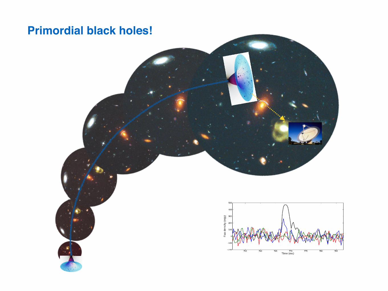
Primordial black holes!

A real-time FRB 5

Figure 2. The full-Stokes parameters of FRB 140514 recorded in the centre beam of the multibeam receiver with BPSR. Total intensity,and Stokes Q, U , and V are represented in black, red, green, and blue, respectively. FRB 140514 has 21 ± 7% (3-�) circular polarisationaveraged over the pulse, and a 1-� upper limit on linear polarisation of L < 10%. On the leading edge of the pulse the circular polarisationis 42 ± 9% (5-�) of the total intensity. The data have been smoothed from an initial sampling of 64 µs using a Gaussian filter of full-widthhalf-maximum 90 µs.

source given the temporal proximity of the GMRT observa-tion and the FRB detection. The other two sources, GMRT2and GMRT3, correlated well with positions for known ra-dio sources in the NVSS catalog with consistent flux densi-ties. Subsequent observations were taken through the GMRTToO queue on 20 May, 3 June, and 8 June in the 325 MHz,1390 MHz, and 610 MHz bands, respectively. The secondepoch was largely unusable due to technical di�culties. Thesearch for variablility focused on monitoring each source forflux variations across observing epochs. All sources from thefirst epoch appeared in the third and fourth epochs with nomeasureable change in flux densities.

4.4 Swift X-Ray Telescope

The first observation of the FRB 140514 field was taken us-ing Swift XRT (Gehrels et al. 2004) only 8.5 hours after theFRB was discovered at Parkes. This was the fastest Swiftfollow-up ever undertaken for an FRB. 4 ks of XRT datawere taken in the first epoch, and a further 2 ks of datawere taken in a second epoch later that day, 23 hours af-ter FRB 140514, to search for short term variability. A finalepoch, 18 days later, was taken to search for long term vari-ability. Two X-ray sources were identified in the first epochof data within the 150 diameter of the Parkes beam. Bothsources were consistent with sources in the USNO catalog(Monet et al. 2003). The first source (XRT1) is located atRA = 22:34:41.49, Dec = -12:21:39.8 with RUSNO = 17.5and the second (XRT2) is located at RA = 22:34:02.33 Dec= -12:08:48.2 with RUSNO = 19.7. Both XRT1 and XRT2appeared in all subsequent epochs with no observable vari-ability on the level of 10% and 20% for XRT1 and XRT2,respectively, both calculated from photon counts from theXRT. Both sources were later found to be active galacticnuclei (AGN).

4.5 Gamma-Ray Burst Optical/Near-InfraredDetector

After 13 hours, a trigger was sent to the Gamma-Ray BurstOptical/Near-Infrared Detector (GROND) operating on the2.2-m MPI/ESO telescope on La Silla in Chile (Greiner et al.2008). GROND is able to observe simultaneously in J , H,and K near-infrared (NIR) bands with a 100 ⇥ 100 field ofview (FOV) and the optical g0, r0, i0, and z0 bands with a60 ⇥ 60 FOV. A 2⇥2 tiling observation was done, providing61% (JHK) and 22% (g0r0i0z0) coverage of the inner partof the FRB error circle. The first epoch began 16 hours af-ter FRB 140514 with 460 second exposures, and a secondepoch was taken 2.5 days after the FRB with an identicalobserving setup and 690 s (g0r0i0z0) and 720 s (JHK) ex-posures, respectively. Limiting magnitudes for J , H, and Kbands were 21.1, 20.4, and 18.4 in the first epoch and 21.1,20.5, and 18.6 in the second epoch, respectively (all in theAB system). Of all the objects in the field, analysis iden-tified three variable objects, all very close to the limitingmagnitude and varying on scales of 0.2 - 0.8 mag in the NIRbands identified with di↵erence imaging. Of the three ob-jects one is a galaxy, another is likely to be an AGN, andthe last is a main sequence star. Both XRT1 and GMRT1sources were also detected in the GROND infrared imagingbut were not observed to vary in the infrared bands on thetimescales probed.

4.6 Swope Telescope

An optical image of the FRB field was taken 16h51m afterthe burst event with the 1-m Swope Telescope at Las Cam-panas. The field was re-imaged with the Swope Telescope on17 May, 2 days after the FRB. No variable optical sources

c� 0000 RAS, MNRAS 000, 000–000

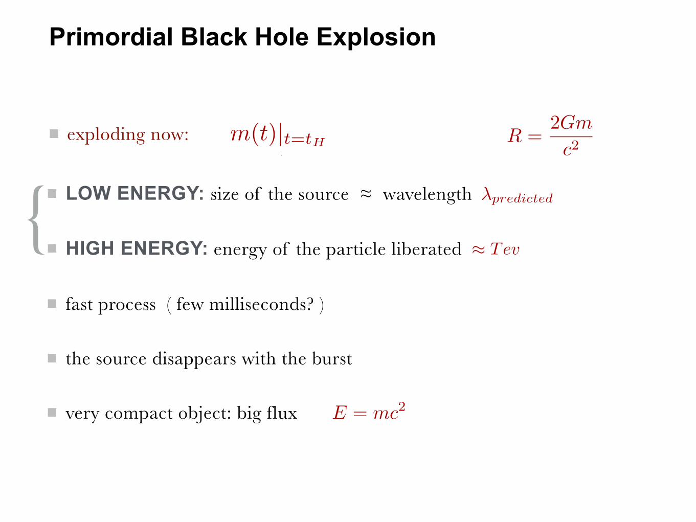
LOW ENERGY: size of the source ≈ wavelength

HIGH ENERGY: energy of the particle liberated

fast process ( few milliseconds? )

the source disappears with the burst

very compact object: big flux E = mc2 ⇠ 1.7⇥ 1047 erg

�predicted & .02 cm

exploding now: R =2Gm

c2⇠ .02 cmm =

rtH4k

⇠ 1.2⇥ 1023 kg

{⇡ Tev

Primordial Black Hole Explosion

m(t)|t=tH

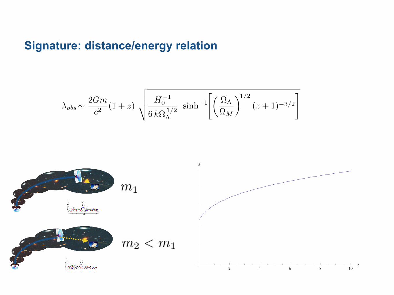
Signature: distance/energy relation

�obs

⇠ 2Gm

c2(1 + z)

vuut H�10

6 k⌦ 1/2⇤

sinh�1

"✓⌦⇤

⌦M

◆1/2

(z + 1)�3/2

#

2

2 4 6 8 10z

l

FIG. 1: White hole signal wavelength (unspecified units) asa function of z. Notice the characteristic flattening at largedistance: the youth of the hole compensate for the redshift.

The received signal is going to be corrected by standardcosmological redshift. However, signals coming form far-ther away were originated earlier, namely by younger,and therefore less massive, holes, giving a peculiar de-crease of the emitted wavelength with distance. The re-ceived wavelength, taking into account both the expan-sion of the universe and the change of time available forthe black hole to bounce, can be obtained folding (1) intothe standard cosmological relation between redshift andproper time. A straightforward calculation gives

�obs ⇠ 2Gm

c2(1 + z) ⇥ (6)

vuut H�10

6 k⌦ 1/2⇤

sinh�1

"✓⌦⇤

⌦M

◆1/2

(z + 1)�3/2

#.

where we have reinserted the Newton constant G andthe speed of light c while H0,⌦⇤ and ⌦M are the Hub-ble constant, the cosmological constant, and the matterdensity. This is a very slowly varying function of theredshift. The e↵ect of the hole’s age almost compesatesfor the red-shift. The signal, indeed, varies by less thanan order of magnitude for redshifts up to the decouplingtime (z=1100). See Figure 1.

If the redshift of the source can be estimated by usingdispersion measures or by identifying a host galaxy, givensu�cient statistics this flattening represents a decisivesignature of the phenomenon we are describing.

Do we have experiments searching for these signals?There are detectors operating at such wavelengths, begin-ning by the recently launched Herschel instrument. The200 micron range can be observed both by PACS (twobolometer arrays and two Ge:Ga photoconductor arrays)and SPIRE (a camera associated with a low to mediumresolution spectrometer). The predicted signal falls in be-tween PACS and SPIRE sensitivity zones. There is also avery high resolution heterodyne spectrometer, HIFI, on-board Herschel, but this is not an imaging instrument, itobserves a single pixel on the sky at a time. However, thebolometer technology makes detecting short white-holebursts di�cult. Cosmic rays cross the detectors very of-ten and induce glitches that are removed from the data.Were physical IR bursts due to bouncing black hole regis-tered by the instrument, they would most probably havebeen flagged and deleted, mimicking a mere cosmic ray

noise. There might be room for improvement. It is notimpossible that the time structure of the bounce couldlead to a characteristic time-scale of the event larger thanthe response time of the bolometer. In that case, aspecific analysis should allow for a dedicated search ofsuch events. We leave this study for a future work asit requires astrophysical considerations beyond this firstinvestigation. An isotropic angular distribution of thebursts, signifying their cosmological origin, could also beconsidered as an evidence for the model. In case manyevents were measured, it would be important to ensurethat there is no correlation with the mean cosmic-ray flux(varying with the solar activity) at the satellite location.Let us turn to something that has been observed.Fast Radio Bursts. Fast Radio Bursts are intense iso-

lated astrophysical radio signals with milliseconds dura-tion. A small number of these were initially detectedonly at the Parkes radio telescope [39–41]. Observationsfrom the Arecibo Observatory have confirmed the detec-tion [42]. The frequency of these signals around 1.3 GHz,namely a wavelength

�observed ⇠ 20 cm. (7)

These signals are believed to be of extragalactic origin,because the observed delay of the signal arrival time withfrequency agrees well with the dispersion due to ionizedmedium as expected from a distant source. The totalenergy emitted in the radio is estimated to be of theorder 1038 erg. The progenitors and physical nature ofthe Fast Radio Bursts are currently unknown [42].There are three orders of magnitude between the pre-

dicted signal (5) and the observed signal (7). But theblack-to-white hole transition model is still very rough. Itdisregards rotation, dissipative phenomena, anisotropies,and other phenomena, and these could account for thediscrepancy.In particular, astrophysical black holes rotate: one may

expect the centrifugal force to lower the attraction andbring the lifetime of the hole down. This should allowlarger black holes to explode today, and signals of largerwavelength. Also, we have not taken the astrophysics ofthe explosion into account. The total energy (3) avail-able in the black hole is largely su�cient –9 orders ofmagnitude larger– than the total energy emitted in theradio estimated by the astronomers.Given these uncertainties, the hypothesis that Fast Ra-

dio Burst could originate from exploding white holes istempting and deserves to be explored.High energy signal. When a black hole radiates by

the Hawking mechanism, its Schwarzschild radius is theonly scale in the problem and the emitted radiation hasa typical wavelength of this size. In the model we areconsidering, the emitted particles do not come from thecoupling of the event horizon with the vacuum quan-tum fluctuations, but rather from the time-reversal ofthe phenomenon that formed (and filled) the black hole.Therefore the emitted signal is characterized by second

A real-time FRB 5

Figure 2. The full-Stokes parameters of FRB 140514 recorded in the centre beam of the multibeam receiver with BPSR. Total intensity,and Stokes Q, U , and V are represented in black, red, green, and blue, respectively. FRB 140514 has 21 ± 7% (3-�) circular polarisationaveraged over the pulse, and a 1-� upper limit on linear polarisation of L < 10%. On the leading edge of the pulse the circular polarisationis 42 ± 9% (5-�) of the total intensity. The data have been smoothed from an initial sampling of 64 µs using a Gaussian filter of full-widthhalf-maximum 90 µs.

source given the temporal proximity of the GMRT observa-tion and the FRB detection. The other two sources, GMRT2and GMRT3, correlated well with positions for known ra-dio sources in the NVSS catalog with consistent flux densi-ties. Subsequent observations were taken through the GMRTToO queue on 20 May, 3 June, and 8 June in the 325 MHz,1390 MHz, and 610 MHz bands, respectively. The secondepoch was largely unusable due to technical di�culties. Thesearch for variablility focused on monitoring each source forflux variations across observing epochs. All sources from thefirst epoch appeared in the third and fourth epochs with nomeasureable change in flux densities.

4.4 Swift X-Ray Telescope

The first observation of the FRB 140514 field was taken us-ing Swift XRT (Gehrels et al. 2004) only 8.5 hours after theFRB was discovered at Parkes. This was the fastest Swiftfollow-up ever undertaken for an FRB. 4 ks of XRT datawere taken in the first epoch, and a further 2 ks of datawere taken in a second epoch later that day, 23 hours af-ter FRB 140514, to search for short term variability. A finalepoch, 18 days later, was taken to search for long term vari-ability. Two X-ray sources were identified in the first epochof data within the 150 diameter of the Parkes beam. Bothsources were consistent with sources in the USNO catalog(Monet et al. 2003). The first source (XRT1) is located atRA = 22:34:41.49, Dec = -12:21:39.8 with RUSNO = 17.5and the second (XRT2) is located at RA = 22:34:02.33 Dec= -12:08:48.2 with RUSNO = 19.7. Both XRT1 and XRT2appeared in all subsequent epochs with no observable vari-ability on the level of 10% and 20% for XRT1 and XRT2,respectively, both calculated from photon counts from theXRT. Both sources were later found to be active galacticnuclei (AGN).

4.5 Gamma-Ray Burst Optical/Near-InfraredDetector

After 13 hours, a trigger was sent to the Gamma-Ray BurstOptical/Near-Infrared Detector (GROND) operating on the2.2-m MPI/ESO telescope on La Silla in Chile (Greiner et al.2008). GROND is able to observe simultaneously in J , H,and K near-infrared (NIR) bands with a 100 ⇥ 100 field ofview (FOV) and the optical g0, r0, i0, and z0 bands with a60 ⇥ 60 FOV. A 2⇥2 tiling observation was done, providing61% (JHK) and 22% (g0r0i0z0) coverage of the inner partof the FRB error circle. The first epoch began 16 hours af-ter FRB 140514 with 460 second exposures, and a secondepoch was taken 2.5 days after the FRB with an identicalobserving setup and 690 s (g0r0i0z0) and 720 s (JHK) ex-posures, respectively. Limiting magnitudes for J , H, and Kbands were 21.1, 20.4, and 18.4 in the first epoch and 21.1,20.5, and 18.6 in the second epoch, respectively (all in theAB system). Of all the objects in the field, analysis iden-tified three variable objects, all very close to the limitingmagnitude and varying on scales of 0.2 - 0.8 mag in the NIRbands identified with di↵erence imaging. Of the three ob-jects one is a galaxy, another is likely to be an AGN, andthe last is a main sequence star. Both XRT1 and GMRT1sources were also detected in the GROND infrared imagingbut were not observed to vary in the infrared bands on thetimescales probed.

4.6 Swope Telescope

An optical image of the FRB field was taken 16h51m afterthe burst event with the 1-m Swope Telescope at Las Cam-panas. The field was re-imaged with the Swope Telescope on17 May, 2 days after the FRB. No variable optical sources

c� 0000 RAS, MNRAS 000, 000–000

A real-time FRB 5

Figure 2. The full-Stokes parameters of FRB 140514 recorded in the centre beam of the multibeam receiver with BPSR. Total intensity,and Stokes Q, U , and V are represented in black, red, green, and blue, respectively. FRB 140514 has 21 ± 7% (3-�) circular polarisationaveraged over the pulse, and a 1-� upper limit on linear polarisation of L < 10%. On the leading edge of the pulse the circular polarisationis 42 ± 9% (5-�) of the total intensity. The data have been smoothed from an initial sampling of 64 µs using a Gaussian filter of full-widthhalf-maximum 90 µs.

source given the temporal proximity of the GMRT observa-tion and the FRB detection. The other two sources, GMRT2and GMRT3, correlated well with positions for known ra-dio sources in the NVSS catalog with consistent flux densi-ties. Subsequent observations were taken through the GMRTToO queue on 20 May, 3 June, and 8 June in the 325 MHz,1390 MHz, and 610 MHz bands, respectively. The secondepoch was largely unusable due to technical di�culties. Thesearch for variablility focused on monitoring each source forflux variations across observing epochs. All sources from thefirst epoch appeared in the third and fourth epochs with nomeasureable change in flux densities.

4.4 Swift X-Ray Telescope

The first observation of the FRB 140514 field was taken us-ing Swift XRT (Gehrels et al. 2004) only 8.5 hours after theFRB was discovered at Parkes. This was the fastest Swiftfollow-up ever undertaken for an FRB. 4 ks of XRT datawere taken in the first epoch, and a further 2 ks of datawere taken in a second epoch later that day, 23 hours af-ter FRB 140514, to search for short term variability. A finalepoch, 18 days later, was taken to search for long term vari-ability. Two X-ray sources were identified in the first epochof data within the 150 diameter of the Parkes beam. Bothsources were consistent with sources in the USNO catalog(Monet et al. 2003). The first source (XRT1) is located atRA = 22:34:41.49, Dec = -12:21:39.8 with RUSNO = 17.5and the second (XRT2) is located at RA = 22:34:02.33 Dec= -12:08:48.2 with RUSNO = 19.7. Both XRT1 and XRT2appeared in all subsequent epochs with no observable vari-ability on the level of 10% and 20% for XRT1 and XRT2,respectively, both calculated from photon counts from theXRT. Both sources were later found to be active galacticnuclei (AGN).

4.5 Gamma-Ray Burst Optical/Near-InfraredDetector

After 13 hours, a trigger was sent to the Gamma-Ray BurstOptical/Near-Infrared Detector (GROND) operating on the2.2-m MPI/ESO telescope on La Silla in Chile (Greiner et al.2008). GROND is able to observe simultaneously in J , H,and K near-infrared (NIR) bands with a 100 ⇥ 100 field ofview (FOV) and the optical g0, r0, i0, and z0 bands with a60 ⇥ 60 FOV. A 2⇥2 tiling observation was done, providing61% (JHK) and 22% (g0r0i0z0) coverage of the inner partof the FRB error circle. The first epoch began 16 hours af-ter FRB 140514 with 460 second exposures, and a secondepoch was taken 2.5 days after the FRB with an identicalobserving setup and 690 s (g0r0i0z0) and 720 s (JHK) ex-posures, respectively. Limiting magnitudes for J , H, and Kbands were 21.1, 20.4, and 18.4 in the first epoch and 21.1,20.5, and 18.6 in the second epoch, respectively (all in theAB system). Of all the objects in the field, analysis iden-tified three variable objects, all very close to the limitingmagnitude and varying on scales of 0.2 - 0.8 mag in the NIRbands identified with di↵erence imaging. Of the three ob-jects one is a galaxy, another is likely to be an AGN, andthe last is a main sequence star. Both XRT1 and GMRT1sources were also detected in the GROND infrared imagingbut were not observed to vary in the infrared bands on thetimescales probed.

4.6 Swope Telescope

An optical image of the FRB field was taken 16h51m afterthe burst event with the 1-m Swope Telescope at Las Cam-panas. The field was re-imaged with the Swope Telescope on17 May, 2 days after the FRB. No variable optical sources

c� 0000 RAS, MNRAS 000, 000–000

⌧ ⇠ m3k=1012 k=1016

k=1019 k=1022

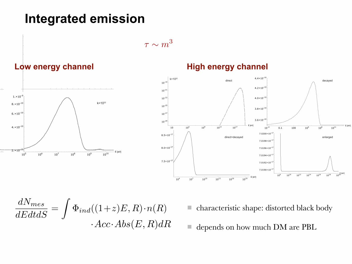
Integrated emission

Low energy channel High energy channelk=1022 direct decayed

direct+decayed enlarged

characteristic shape: distorted black body

depends on how much DM are PBL

�meashigh ⇠ 2⇡

kBT

(1 + z)

(0.3g�1⇤

)12

"H�1

0

6k⌦1/2⇤

sinh�1

"✓⌦⇤

⌦M

◆ 12

(1 + z)�32

## 14

. (6)

This shows that although the mean wavelength doesdecreases as a function of k in both cases, it does notfollow the same general behavior. It scales with k�

12

for the low energy component and as k�14 for the high

energy one.

The following conclusions can be drawn:

• The low energy channel leads to a better single-event detection than the high energy channel.Although lower energy dilutes the signal in ahigher astrophysical background, this e↵ect is over-compensated by the larger amount of photons.

• The di↵erence of maximal distances between thelow- and high energy channels decreases for highervalues of k, i.e. for longer black-hole lifetimes.

• In the low energy channel, for the smaller valuesof k, a single bounce can be detected arbitrary faraway in the Universe.

• In all cases, the distances are large enough and ex-perimental detection is far from being hopeless.

III. INTEGRATED EMISSION

In addition to the instantaneous spectrum emitted by asingle bouncing black hole, it is interesting to consider thepossible di↵use background due to the integrated emis-sion of a population of bouncing black holes. Formally,the number of measured photons detected per unit time,unit energy and unit surface, can be written as:

dNmes

dEdtdS=

Z�ind((1+z)E,R)·n(R)·Acc·Abs(E,R)dR,

(7)where �ind(E,R) denotes the individual flux emittedby a single bouncing black hole at distance R and atenergy E, Acc is the angular acceptance of the detectormultiplied by its e�ciency (in principle this is also afunction of E but this will be ignored here), Abs(E,R)is the absorption function, and n(R) is the number ofblack holes bouncing at distance R per unit time andvolume. The distance R and the redshift z enteringthe above formula are linked. The integration has tobe carried out up to cosmological distances and it istherefore necessary to use exact results behind the linearapproximation. The energy is also correlated with Ras the distance fixes the bounce time of the black holewhich, subsequently, fixes the emitted energy.

It is worth considering the n(R) term a bit more indetail. If one denotes by dn

dMdV the initial di↵erentialmass spectrum of primordial black holes per unit volume,it is possible to define n(R) as:

n(R) =

Z M(t+�t)

M(t)

dn

dMdVdM, (8)

leading to

n(R) ⇡ dn

dMdV

�t

8k, (9)

where the mass spectrum is evaluated for the mass cor-responding to a time (tH � R

c ). If one assumes that pri-mordial black holes are directly formed by the collapseof density fluctuations with a high-enough density con-trast in the early Universe, the initial mass spectrum isdirectly related to the equation of state of the Universeat the formation epoch. It is given by [18, 19]:

dn

dMdV= ↵M�1� 1+3w

1+w , (10)

where w = p/⇢. In a matter-dominated universe theexponent � ⌘ �1 � 1+3w

1+w takes the value � = �5/2.The normalization coe�cient ↵ will be kept unknownas it depends on the details of the black hole formationmechanism. For a sizeable amount of primordial blackholes to form, the power spectrum normalized on theCMB needs to be boosted at small scales. This canbe achieved, for example, through Staobinsky’s brokenscale invariance (BSI) scenario. The idea is that themass spectrum takes a high enough value in the relevantrange whereas it is naturally suppressed at small massesby inflation and at large masses by the BSI hypothesis.We will not study those questions here and just considerthe shape of the resulting emission, nor its normalisationwhich depends sensitively on the bounds of the massspectrum, that are highly model-dependent. As this partof the study is devoted to the investigation of the shapeof the signal, the y axis on the figures are not normalized.

Fortunately, the results are weakly dependent uponthe shape of the mass spectrum. This is illustrated inFig. 5 where di↵erent hypothesis for the exponent � aredisplayed. The resulting electromagnetic spectrum isalmost exactly the same. Therefore we only keep onecase (� = �5/2, corresponding to w = 1/3). The blackholes are assumed to be uniformly distributed in theUniverse, which is a meaningful hypothesis as long as

5

�meashigh ⇠ 2⇡

kBT

(1 + z)

(0.3g�1⇤

)12

"H�1

0

6k⌦1/2⇤

sinh�1

"✓⌦⇤

⌦M

◆ 12

(1 + z)�32

## 14

. (6)

This shows that although the mean wavelength doesdecreases as a function of k in both cases, it does notfollow the same general behavior. It scales with k�

12

for the low energy component and as k�14 for the high

energy one.

The following conclusions can be drawn:

• The low energy channel leads to a better single-event detection than the high energy channel.Although lower energy dilutes the signal in ahigher astrophysical background, this e↵ect is over-compensated by the larger amount of photons.

• The di↵erence of maximal distances between thelow- and high energy channels decreases for highervalues of k, i.e. for longer black-hole lifetimes.

• In the low energy channel, for the smaller valuesof k, a single bounce can be detected arbitrary faraway in the Universe.

• In all cases, the distances are large enough and ex-perimental detection is far from being hopeless.

III. INTEGRATED EMISSION

In addition to the instantaneous spectrum emitted by asingle bouncing black hole, it is interesting to consider thepossible di↵use background due to the integrated emis-sion of a population of bouncing black holes. Formally,the number of measured photons detected per unit time,unit energy and unit surface, can be written as:

dNmes

dEdtdS=

Z�ind((1+z)E,R)·n(R)·Acc·Abs(E,R)dR,

(7)where �ind(E,R) denotes the individual flux emittedby a single bouncing black hole at distance R and atenergy E, Acc is the angular acceptance of the detectormultiplied by its e�ciency (in principle this is also afunction of E but this will be ignored here), Abs(E,R)is the absorption function, and n(R) is the number ofblack holes bouncing at distance R per unit time andvolume. The distance R and the redshift z enteringthe above formula are linked. The integration has tobe carried out up to cosmological distances and it istherefore necessary to use exact results behind the linearapproximation. The energy is also correlated with Ras the distance fixes the bounce time of the black holewhich, subsequently, fixes the emitted energy.

It is worth considering the n(R) term a bit more indetail. If one denotes by dn

dMdV the initial di↵erentialmass spectrum of primordial black holes per unit volume,it is possible to define n(R) as:

n(R) =

Z M(t+�t)

M(t)

dn

dMdVdM, (8)

leading to

n(R) ⇡ dn

dMdV

�t

8k, (9)

where the mass spectrum is evaluated for the mass cor-responding to a time (tH � R

c ). If one assumes that pri-mordial black holes are directly formed by the collapseof density fluctuations with a high-enough density con-trast in the early Universe, the initial mass spectrum isdirectly related to the equation of state of the Universeat the formation epoch. It is given by [18, 19]:

dn

dMdV= ↵M�1� 1+3w

1+w , (10)

where w = p/⇢. In a matter-dominated universe theexponent � ⌘ �1 � 1+3w

1+w takes the value � = �5/2.The normalization coe�cient ↵ will be kept unknownas it depends on the details of the black hole formationmechanism. For a sizeable amount of primordial blackholes to form, the power spectrum normalized on theCMB needs to be boosted at small scales. This canbe achieved, for example, through Staobinsky’s brokenscale invariance (BSI) scenario. The idea is that themass spectrum takes a high enough value in the relevantrange whereas it is naturally suppressed at small massesby inflation and at large masses by the BSI hypothesis.We will not study those questions here and just considerthe shape of the resulting emission, nor its normalisationwhich depends sensitively on the bounds of the massspectrum, that are highly model-dependent. As this partof the study is devoted to the investigation of the shapeof the signal, the y axis on the figures are not normalized.

Fortunately, the results are weakly dependent uponthe shape of the mass spectrum. This is illustrated inFig. 5 where di↵erent hypothesis for the exponent � aredisplayed. The resulting electromagnetic spectrum isalmost exactly the same. Therefore we only keep onecase (� = �5/2, corresponding to w = 1/3). The blackholes are assumed to be uniformly distributed in theUniverse, which is a meaningful hypothesis as long as

5

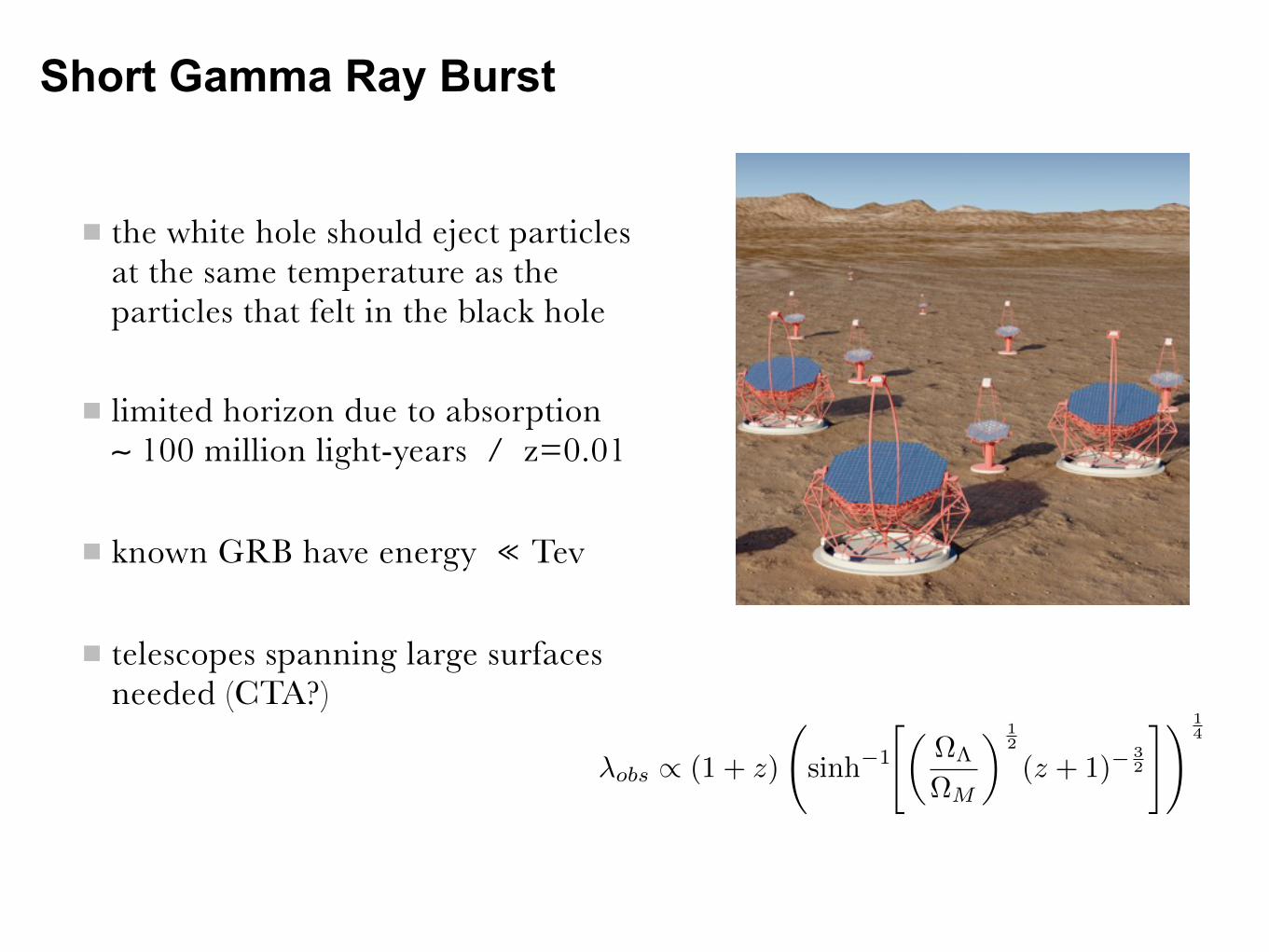
Short Gamma Ray Burst

the white hole should eject particles at the same temperature as the particles that felt in the black hole

limited horizon due to absorption ∼ 100 million light-years / z=0.01

known GRB have energy ≪ Tev

telescopes spanning large surfaces needed (CTA?)

�obs

/ (1 + z)

sinh�1

"✓⌦⇤

⌦M

◆ 12

(z + 1)�32

#! 14

Fast Radio Burst

A real-time FRB 5

Figure 2. The full-Stokes parameters of FRB 140514 recorded in the centre beam of the multibeam receiver with BPSR. Total intensity,and Stokes Q, U , and V are represented in black, red, green, and blue, respectively. FRB 140514 has 21 ± 7% (3-�) circular polarisationaveraged over the pulse, and a 1-� upper limit on linear polarisation of L < 10%. On the leading edge of the pulse the circular polarisationis 42 ± 9% (5-�) of the total intensity. The data have been smoothed from an initial sampling of 64 µs using a Gaussian filter of full-widthhalf-maximum 90 µs.

source given the temporal proximity of the GMRT observa-tion and the FRB detection. The other two sources, GMRT2and GMRT3, correlated well with positions for known ra-dio sources in the NVSS catalog with consistent flux densi-ties. Subsequent observations were taken through the GMRTToO queue on 20 May, 3 June, and 8 June in the 325 MHz,1390 MHz, and 610 MHz bands, respectively. The secondepoch was largely unusable due to technical di�culties. Thesearch for variablility focused on monitoring each source forflux variations across observing epochs. All sources from thefirst epoch appeared in the third and fourth epochs with nomeasureable change in flux densities.

4.4 Swift X-Ray Telescope

The first observation of the FRB 140514 field was taken us-ing Swift XRT (Gehrels et al. 2004) only 8.5 hours after theFRB was discovered at Parkes. This was the fastest Swiftfollow-up ever undertaken for an FRB. 4 ks of XRT datawere taken in the first epoch, and a further 2 ks of datawere taken in a second epoch later that day, 23 hours af-ter FRB 140514, to search for short term variability. A finalepoch, 18 days later, was taken to search for long term vari-ability. Two X-ray sources were identified in the first epochof data within the 150 diameter of the Parkes beam. Bothsources were consistent with sources in the USNO catalog(Monet et al. 2003). The first source (XRT1) is located atRA = 22:34:41.49, Dec = -12:21:39.8 with RUSNO = 17.5and the second (XRT2) is located at RA = 22:34:02.33 Dec= -12:08:48.2 with RUSNO = 19.7. Both XRT1 and XRT2appeared in all subsequent epochs with no observable vari-ability on the level of 10% and 20% for XRT1 and XRT2,respectively, both calculated from photon counts from theXRT. Both sources were later found to be active galacticnuclei (AGN).

4.5 Gamma-Ray Burst Optical/Near-InfraredDetector

After 13 hours, a trigger was sent to the Gamma-Ray BurstOptical/Near-Infrared Detector (GROND) operating on the2.2-m MPI/ESO telescope on La Silla in Chile (Greiner et al.2008). GROND is able to observe simultaneously in J , H,and K near-infrared (NIR) bands with a 100 ⇥ 100 field ofview (FOV) and the optical g0, r0, i0, and z0 bands with a60 ⇥ 60 FOV. A 2⇥2 tiling observation was done, providing61% (JHK) and 22% (g0r0i0z0) coverage of the inner partof the FRB error circle. The first epoch began 16 hours af-ter FRB 140514 with 460 second exposures, and a secondepoch was taken 2.5 days after the FRB with an identicalobserving setup and 690 s (g0r0i0z0) and 720 s (JHK) ex-posures, respectively. Limiting magnitudes for J , H, and Kbands were 21.1, 20.4, and 18.4 in the first epoch and 21.1,20.5, and 18.6 in the second epoch, respectively (all in theAB system). Of all the objects in the field, analysis iden-tified three variable objects, all very close to the limitingmagnitude and varying on scales of 0.2 - 0.8 mag in the NIRbands identified with di↵erence imaging. Of the three ob-jects one is a galaxy, another is likely to be an AGN, andthe last is a main sequence star. Both XRT1 and GMRT1sources were also detected in the GROND infrared imagingbut were not observed to vary in the infrared bands on thetimescales probed.

4.6 Swope Telescope

An optical image of the FRB field was taken 16h51m afterthe burst event with the 1-m Swope Telescope at Las Cam-panas. The field was re-imaged with the Swope Telescope on17 May, 2 days after the FRB. No variable optical sources

c� 0000 RAS, MNRAS 000, 000–000

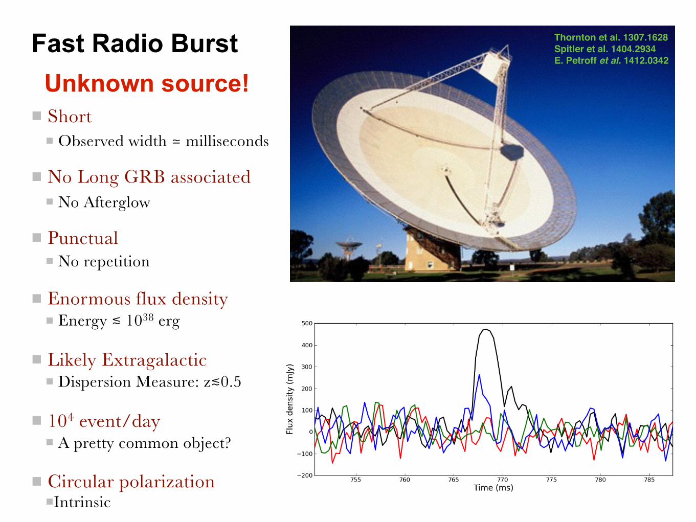
Thornton et al. 1307.1628 Spitler et al. 1404.2934 E. Petroff et al. 1412.0342

Unknown source!

Observed width ≃ milliseconds

No Afterglow

No repetition

Energy ≲ 1038 erg

Dispersion Measure: z≲0.5

A pretty common object?

Intrinsic

Short

No Long GRB associated

Punctual

Enormous flux density

Likely Extragalactic

104 event/day

Circular polarization

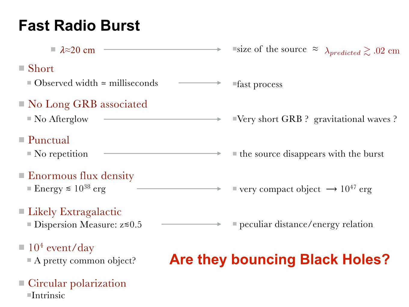
size of the source ≈

fast process

Very short GRB ? gravitational waves ?

the source disappears with the burst

very compact object ⟶ 1047 erg

peculiar distance/energy relation

Observed width ≃ milliseconds

No Afterglow

No repetition

Energy ≲ 1038 erg

Dispersion Measure: z≲0.5

A pretty common object?

Intrinsic

Fast Radio Burst

Are they bouncing Black Holes?

�predicted & .02 cm

Short

No Long GRB associated

Punctual

Enormous flux density

Likely Extragalactic

104 event/day

Circular polarization

𝜆≈20 cm

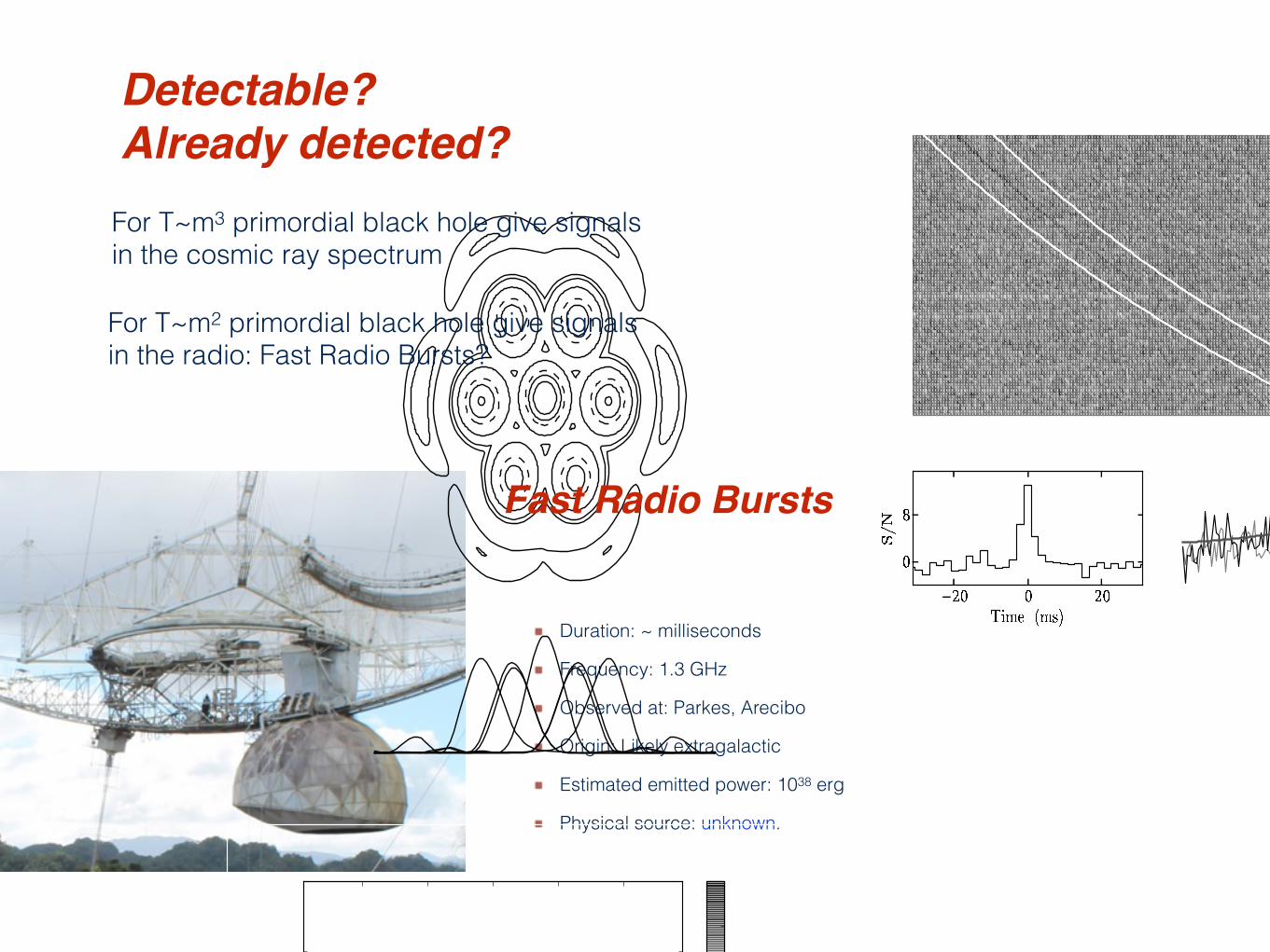
Detectable?Already detected?

Duration: ~ milliseconds

Frequency: 1.3 GHz

Observed at: Parkes, Arecibo

Origin: Likely extragalactic

Estimated emitted power: 1038 erg

Physical source: unknown.

4

Figure 1. Gain and spectral index maps for the ALFA receiver.Figure a): Contour plot of the ALFA power pattern calculatedfrom the model described in Section 3 at ν = 1375 MHz. Thecontour levels are −13, −10, −6, −3 (dashed), −2, and −1 dB(top panel). The bottom inset shows slices in azimuth for eachbeam, and each slice passes through the peak gain for its respec-tive beam. Beam 1 is in the upper right, and the beam number-ing proceeds clockwise. Beam 4 is, therefore, in the lower left.Figure b): Map of the apparent instrumental spectral index dueto frequency-dependent gain variations of ALFA. The spectral in-dexes were calculated at the center frequencies of each subband.Only pixels with gain > 0.5 K Jy−1 were used in the calculation.The rising edge of the first sidelobe can impart a positive appar-ent spectral index with a magnitude that is consistent with themeasured spectral index of FRB 121102.

of parameters. The model assumes a Gaussian pulseprofile convolved with a one-sided exponential scatter-ing tail. The amplitude of the Gaussian is scaled witha spectral index (S(ν) ∝ να), and the temporal loca-tion of the pulse was modeled as an absolute arrival timeplus dispersive delay. For the least-squares fitting theDM was held constant, and the spectral index of τd wasfixed to be −4.4. The Gaussian FWHM pulse width,the spectral index, Gaussian amplitude, absolute arrival

Figure 2. Characteristic plots of FRB 121102. In each panel thedata were smoothed in time and frequency by a factor of 30 and 10,respectively. The top panel is a dynamic spectrum of the discov-ery observation showing the 0.7 s during which FRB 121102 sweptacross the frequency band. The signal is seen to become signifi-cantly dimmer towards the lower part of the band, and some arti-facts due to RFI are also visible. The two white curves show the ex-pected sweep for a ν−2 dispersed signal at a DM = 557.4 pc cm−3.The lower left panel shows the dedispersed pulse profile averagedacross the bandpass. The lower right panel compares the on-pulsespectrum (black) with an off-pulse spectrum (light gray), and forreference a curve showing the fitted spectral index (α = 10) is alsooverplotted (medium gray). The on-pulse spectrum was calculatedby extracting the frequency channels in the dedispersed data cor-responding to the peak in the pulse profile. The off-pulse spectrumis the extracted frequency channels for a time bin manually chosento be far from the pulse.

time, and pulsar broadening were all fitted. The Gaus-sian pulse width (FWHM) is 3.0 ± 0.5 ms, and we foundan upper limit of τd < 1.5 ms at 1.4 GHz. The residualDM smearing within a frequency channel is 0.5 ms and0.9ms at the top and bottom of the band, respectively.The best-fit value was α = 11 but could be as low as α= 7. The fit for α is highly covariant with the Gaussianamplitude.Every PALFA observation yields many single-pulse

events that are not associated with astrophysical sig-nals. A well-understood source of events is false positivesfrom Gaussian noise. These events are generally isolated(i.e. no corresponding event in neighboring trial DMs),have low S/Ns, and narrow temporal widths. RFI canalso generate a large number of events, some of whichmimic the properties of astrophysical signals. Nonethe-less, these can be distinguished from astrophysical pulsesin a number of ways. For example, RFI may peak in S/Nat DM = 0pc cm−3, whereas astrophysical pulses peakat a DM > 0 pc cm−3. Although both impulsive RFIand an astrophysical pulse may span a wide range oftrial DMs, the RFI will likely show no clear correlationof S/N with trial DM, while the astrophysical pulse willhave a fairly symmetric reduction in S/N for trial DMsjust below and above the peak value. RFI may be seensimultaneously in multiple, non-adjacent beams, while abright, astrophysical signal may only be seen in only onebeam or multiple, adjacent beams. FRB 121102 exhib-ited all of the characteristics expected for a broadband,dispersed pulse, and therefore clearly stood out from allother candidate events that appeared in the pipeline out-put for large DMs.

For T~m3 primordial black hole give signals in the cosmic ray spectrum

For T~m2 primordial black hole give signals in the radio: Fast Radio Bursts?

Fast Radio Bursts

➜

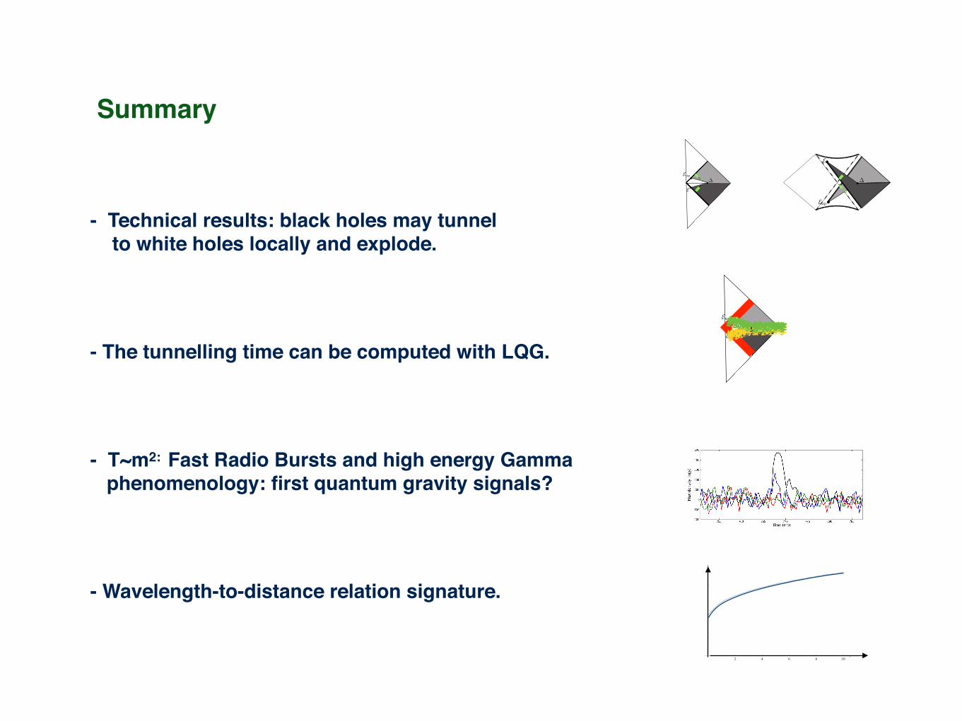
Summary

- Technical results: black holes may tunnel to white holes locally and explode.

- The tunnelling time can be computed with LQG.

- T~m2: Fast Radio Bursts and high energy Gamma phenomenology: first quantum gravity signals?

- Wavelength-to-distance relation signature.

2 4 6 8 10z

l

A real-time FRB 5

Figure 2. The full-Stokes parameters of FRB 140514 recorded in the centre beam of the multibeam receiver with BPSR. Total intensity,and Stokes Q, U , and V are represented in black, red, green, and blue, respectively. FRB 140514 has 21 ± 7% (3-�) circular polarisationaveraged over the pulse, and a 1-� upper limit on linear polarisation of L < 10%. On the leading edge of the pulse the circular polarisationis 42 ± 9% (5-�) of the total intensity. The data have been smoothed from an initial sampling of 64 µs using a Gaussian filter of full-widthhalf-maximum 90 µs.

source given the temporal proximity of the GMRT observa-tion and the FRB detection. The other two sources, GMRT2and GMRT3, correlated well with positions for known ra-dio sources in the NVSS catalog with consistent flux densi-ties. Subsequent observations were taken through the GMRTToO queue on 20 May, 3 June, and 8 June in the 325 MHz,1390 MHz, and 610 MHz bands, respectively. The secondepoch was largely unusable due to technical di�culties. Thesearch for variablility focused on monitoring each source forflux variations across observing epochs. All sources from thefirst epoch appeared in the third and fourth epochs with nomeasureable change in flux densities.

4.4 Swift X-Ray Telescope

The first observation of the FRB 140514 field was taken us-ing Swift XRT (Gehrels et al. 2004) only 8.5 hours after theFRB was discovered at Parkes. This was the fastest Swiftfollow-up ever undertaken for an FRB. 4 ks of XRT datawere taken in the first epoch, and a further 2 ks of datawere taken in a second epoch later that day, 23 hours af-ter FRB 140514, to search for short term variability. A finalepoch, 18 days later, was taken to search for long term vari-ability. Two X-ray sources were identified in the first epochof data within the 150 diameter of the Parkes beam. Bothsources were consistent with sources in the USNO catalog(Monet et al. 2003). The first source (XRT1) is located atRA = 22:34:41.49, Dec = -12:21:39.8 with RUSNO = 17.5and the second (XRT2) is located at RA = 22:34:02.33 Dec= -12:08:48.2 with RUSNO = 19.7. Both XRT1 and XRT2appeared in all subsequent epochs with no observable vari-ability on the level of 10% and 20% for XRT1 and XRT2,respectively, both calculated from photon counts from theXRT. Both sources were later found to be active galacticnuclei (AGN).

4.5 Gamma-Ray Burst Optical/Near-InfraredDetector

After 13 hours, a trigger was sent to the Gamma-Ray BurstOptical/Near-Infrared Detector (GROND) operating on the2.2-m MPI/ESO telescope on La Silla in Chile (Greiner et al.2008). GROND is able to observe simultaneously in J , H,and K near-infrared (NIR) bands with a 100 ⇥ 100 field ofview (FOV) and the optical g0, r0, i0, and z0 bands with a60 ⇥ 60 FOV. A 2⇥2 tiling observation was done, providing61% (JHK) and 22% (g0r0i0z0) coverage of the inner partof the FRB error circle. The first epoch began 16 hours af-ter FRB 140514 with 460 second exposures, and a secondepoch was taken 2.5 days after the FRB with an identicalobserving setup and 690 s (g0r0i0z0) and 720 s (JHK) ex-posures, respectively. Limiting magnitudes for J , H, and Kbands were 21.1, 20.4, and 18.4 in the first epoch and 21.1,20.5, and 18.6 in the second epoch, respectively (all in theAB system). Of all the objects in the field, analysis iden-tified three variable objects, all very close to the limitingmagnitude and varying on scales of 0.2 - 0.8 mag in the NIRbands identified with di↵erence imaging. Of the three ob-jects one is a galaxy, another is likely to be an AGN, andthe last is a main sequence star. Both XRT1 and GMRT1sources were also detected in the GROND infrared imagingbut were not observed to vary in the infrared bands on thetimescales probed.

4.6 Swope Telescope

An optical image of the FRB field was taken 16h51m afterthe burst event with the 1-m Swope Telescope at Las Cam-panas. The field was re-imaged with the Swope Telescope on17 May, 2 days after the FRB. No variable optical sources

c� 0000 RAS, MNRAS 000, 000–000

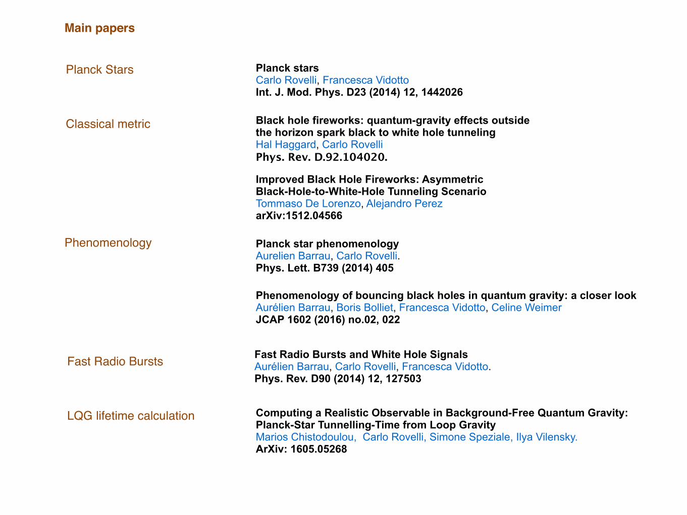
Planck stars Carlo Rovelli, Francesca Vidotto Int. J. Mod. Phys. D23 (2014) 12, 1442026

Computing a Realistic Observable in Background-Free Quantum Gravity: Planck-Star Tunnelling-Time from Loop Gravity Marios Chistodoulou, Carlo Rovelli, Simone Speziale, Ilya Vilensky. ArXiv: 1605.05268

Black hole fireworks: quantum-gravity effects outside the horizon spark black to white hole tunneling Hal Haggard, Carlo Rovelli Phys. Rev. D.92.104020.

Fast Radio Bursts and White Hole Signals Aurélien Barrau, Carlo Rovelli, Francesca Vidotto. Phys. Rev. D90 (2014) 12, 127503

Planck star phenomenology Aurelien Barrau, Carlo Rovelli. Phys. Lett. B739 (2014) 405

Planck Stars

Classical metric

Phenomenology

Fast Radio Bursts

LQG lifetime calculation

Main papers

Phenomenology of bouncing black holes in quantum gravity: a closer look Aurélien Barrau, Boris Bolliet, Francesca Vidotto, Celine Weimer JCAP 1602 (2016) no.02, 022

Improved Black Hole Fireworks: Asymmetric Black-Hole-to-White-Hole Tunneling Scenario Tommaso De Lorenzo, Alejandro Perez arXiv:1512.04566