PJM InterconnectionState of the Market Report

2001

Market Monitoring UnitPJM Interconnection, L.L.C.

June 2002

PJM Interconnection State of the Market Report2001

Contents

Section 1. State of the Market 1Purpose 1PJM Markets 1Conclusions 1Recommendations 2Energy Markets 3Capacity Markets 7Ancillary Services 9Congestion, FTRs and the FTR Auction Market 10

Section 2. Energy Market 13Summary and Conclusions 13Net Revenue 14Price-Cost Mark Up 19Market Structure 25PJM Energy Market Prices 29Appendix 49

Section 3. Capacity Credit Market 69Summary and Conclusions 69Market Fundamentals 70Market Dynamics 73Capacity Market Structure 74Capacity Availability 77Capacity Credit Market Prices 79Capacity Credit Markets in the First Quarter of 2001 81Change in the Allocation of Deficiency Revenues 91Introduction of an Interval Market 93Capacity Market Data 95Appendix 98

Section 4. Ancillary Services 101Summary and Conclusions 101Regulation Service 101The Regulation Market 103Regulation Market Structure 105Regulation Market Results 106Regulation Performance 109Spinning Reserve Service 111

Section 5. Congestion, FTRs and the FTR Auction Market 115Summary and Conclusions 115History 116Congestion Accounting 118Congestion in PJM 118Congestion Details 123PJM FTR Mechanics 127Simultaneous Feasibility Test 127FTR Values 128Acquisition of FTRs 129Network Integration Service FTRs 129Firm Point-to-Point Service FTRs 130Bilateral Market FTRs 130Monthly Auction FTRs 131Results of the FTR Auction 132

1

STATE OF THE MARKET 2001

PurposeThe PJM Interconnection State of the Market Report 2001 evaluates the state of the PJM market,identifies specific issues, and recommends potential enhancements to further improve itscompetitiveness and efficiency.

This report was prepared by the PJM Market Monitoring Unit (MMU) pursuant to Attachment Mto the PJM Open Access Transmission Tariff:

“The Market Monitoring Unit shall prepare and submit to the PJM Board and, ifappropriate, to the PJM Members Committee, periodic (and if required, ad hoc)reports on the state of competition within, and the efficiency of, the PJM Market.”

This report consists of a description of PJM markets, conclusions and recommendations followedby sections covering each of the major market areas in PJM. The report is followed by detailedtechnical sections describing the competitive dynamics in each of the major market areas andincluding more detailed analysis and supporting data.

PJM MarketsPJM operates the day-ahead energy market, the real-time energy market, the daily capacitymarket, the monthly and multi-monthly capacity markets, the regulation market and the monthlyFTR auction market. PJM introduced nodal energy pricing with market-clearing prices on April1, 1998 and nodal, market-clearing prices based on competitive offers on April 1, 1999. PJMimplemented a competitive auction-based FTR market on May 1, 1999. Daily capacity marketswere introduced on January 1, 1999 and were broadened to include monthly and multi-monthlymarkets in mid-1999. PJM implemented the day-ahead energy market and the regulation marketon June 1, 2000. PJM plans to add a market in spinning reserves in 2002. The markets managedby PJM are the focus of this report.

ConclusionsThe MMU concludes that in 2001 the energy markets were reasonably competitive, the capacitymarkets experienced a significant market power issue in the beginning of the year, the regulationmarket was competitive and the FTR auction market was competitive and succeeded in itspurpose of increasing access to FTRs, although additional action is needed to ensure equal accessto FTRs.

The MMU concludes that rule changes implemented by PJM addressed the immediate causes ofmarket power in the capacity market, that the PJM capacity market was reasonably competitivelater in 2001, but that market power remains a serious concern given the extreme inelasticity ofdemand and the high levels of concentration in the capacity credit markets.

The MMU concludes that there are potential threats to competition in the energy, capacity andregulation markets that require ongoing scrutiny and in some cases may require action in order tomaintain competition. Under certain conditions, market participants do possess some ability toexercise market power in PJM markets.

2

RecommendationsThe MMU concludes, based on its analysis, that retention of key market rules and certainenhancements to these market rules are required for continued positive results in PJM marketsand to continue improvements in the functioning of PJM markets. These include:

1. Evaluation of additional actions to increase demand side responsiveness to price in bothenergy and capacity markets and actions to address institutional issues which may inhibitthe evolution of demand side price response.

2. Modification of the FTR allocation method to eliminate any barriers to retail competition.3. Development of an approach to identify areas where transmission expansion investments

would relieve congestion where that congestion may enhance generator market powerand where such investments are needed to support competition.

4. Continued enhancements to the capacity market to stimulate competition, adoption of asingle capacity market design and incorporation of explicit market power mitigation rulesto limit the ability to exercise market power in the capacity market.

5. Retention of the $1,000/MWh bid cap in the PJM energy market and investigation ofother rules changes to reduce the incentives to exercise market power.

6. Retention of the $100/MW bid cap in the PJM regulation market.

PJM is pursuing actions to address the issues raised in these recommendations. Specifically,PJM:

1. Has taken several steps to encourage demand side price responsiveness in the wholesalemarkets.

2. Is actively pursuing a change in the FTR allocation method via the stakeholder process.3. Has begun to address the issue of transmission expansion to relieve congestion to support

competition via the stakeholder process.4. Has modified the capacity market rules to eliminate specific incentives to exercise market

power and to make the market term more consistent with the nature of capacityobligations. PJM is also actively engaged in the stakeholder process to review theexisting capacity market rules.

5. Has consistently supported the retention of bid caps in markets where they are necessaryto limit the exercise of market power.

Based on the experience of the MMU during its third year and its analysis of the PJM markets,the MMU does not recommend any change to the Market Monitoring Unit or the MarketMonitoring Plan at this time.

3

Energy MarketsEnergy Market DesignIn PJM, market participants wishing to buy and sell energy have multiple options. Marketparticipants decide whether to meet their energy needs through self-supply, bilateral purchasesfrom generation owners or market intermediaries, through the day-ahead market or the real-timebalancing, or spot, market. Energy purchases can be made over any time frame frominstantaneous real-time balancing market purchases to long term, multi-year bilateral contracts.Purchases may be made from generation located within or outside the PJM control area. Marketparticipants also decide whether and how to sell the output of their generation assets. Generationowners can sell their output within the PJM control area or outside the control area and can usegeneration to meet their own loads, to sell into the spot market or to sell bilaterally. Generationowners can sell their output over multiple time frames from the real-time spot market to multi-year bilateral arrangements. Market participants can use increment and decrement bids in theday-ahead market to hedge positions or to arbitrage expected price differences between markets.The PJM energy market comprises all types of energy transactions, including the sale orpurchase of energy in spot markets, bilateral markets, forward markets, self-supply, imports andexports.

For the full year, real-time spot market activity averaged 6,563 MW during peak periods and6,395 MW during off peak periods, or 21% of average loads. (Figure 1.) In the day-aheadmarket, spot market activity averaged 4,794 MW on peak and 4,877 MW off peak, or 15% ofaverage loads. The day-ahead market is a financial market and thus may be used to provide ahedge against price fluctuations in the real-time spot market.

Figure 1: 2001 PJM Average Hourly Load and Spot Market Volume

0

5,000

10,000

15,000

20,000

25,000

30,000

35,000

40,000

Jan Feb Mar Apr May Jun Jul Aug Sep Oct Nov Dec

Month

Vol

ume

(MW

)

Average Load Average Spot Volume

4

Market participants can import and export energy in real time in response to price differentials,to fulfill bilateral contracts or to self-supply. PJM was a net importer of energy on a monthlybasis for every month in 2001 (Figure 2). On average, PJM imported 1,131 MW in each hour of2001. Imports and exports respond to market prices. The level of transaction activity illustratesthat the PJM energy market exists in the context of a larger energy market. Imports from thatlarger energy market, in response to PJM prices, served as a source of competition for PJMgeneration and limited the duration of high prices during 2001 high demand periods.

Energy Market ResultsThe PJM day-ahead and real-time market prices are key benchmarks against which marketparticipants measure the results of other types of transactions. The MMU has reviewed keymeasures of market structure and performance for 2001, including net revenue, a price-cost markup index, concentration levels and prices. In addition, the MMU evaluated the performance andpotential of demand side management programs in PJM. Based on that review, the MMUconcludes that the energy market was reasonably competitive in 2001.

Net revenue is a significant indicator of overall market performance. Net revenue measures thecontribution to capital costs paid by loads and received by generators from energy markets, fromcapacity markets, from ancillary services and from operating reserve payments. Net revenue isthus an indicator of the profitability of an investment in generation. In 2001, the net revenuesfrom the energy market, the capacity market, ancillary services and operating reserves wouldhave more than covered the fixed costs of peaking units with operating costs of about $45/MWhwhich ran during all profitable hours. The operating cost of $45/MWh reflects operating costestimates based on the average cost of gas in 2001 and the heat rate for a peaking unit. The

Figure 2: Total Import and Export Volume - 2001

-

500,000

1,000,000

1,500,000

2,000,000

2,500,000

3,000,000

JAN FEB MAR APR MAY JUN JUL AUG SEP OCT NOV DEC

Month

Vol

ume

(MW

h)

Imports Exports Total Net Imports

5

market results in 2001 suggest that the fixed costs of a marginal unit were more than fullycovered by net revenues, recognizing that the estimate of net revenues is an upper bound. Whilemarket results vary from year to year, the results in 2001 reflect both higher energy prices than in2000 and higher capacity market prices that resulted in significant part from the exercise ofmarket power during the first quarter of 2001. The net revenue result is consistent with theconclusion that the energy market was reasonably competitive in 2001.

The price-cost markup is a widely used measure of market power. While there are severalapproaches to this measure, the price-cost markup is defined here as the difference between priceand marginal cost, divided by price. Overall, the data on the price-cost markup are consistentwith the conclusion that the energy market was reasonably competitive in 2001.

Concentration ratios are a summary measure of market shares, a key element of market structure.High concentration ratios mean that a small number of sellers dominate the market while lowconcentration ratios mean that a larger number of sellers share in market sales more equally.Concentration measures must be used carefully in assessing the competitiveness of markets. Lowaggregate market concentration ratios do not establish that a market is competitive, that marketparticipants cannot exercise market power or that concentration is not high in particulargeographical market areas. However, high aggregate market concentration ratios do indicate anincreased potential for market participants to exercise market power. The structural analysisindicates that overall the PJM energy market exhibits moderate market concentration. However,specific geographical areas of the PJM system exhibit moderate to high market concentrationthat may be problematic when transmission constraints exist. There is no evidence that marketpower was exercised in these areas in 2001, primarily due to the load obligations of thegenerators there, but a significant market-power related risk exists going forward should thoseobligations change. In addition, concentration levels in the intermediate and peaking portions ofthe PJM supply curve are relatively high.

The result of market structure and the conduct of individual market entities within that structureis reflected in market prices, termed locational marginal prices (LMPs) in PJM. The overall levelof prices is a good general indicator of market performance, although overall price results mustbe interpreted carefully because of the multiple factors that affect them. For example, overallaverage price levels do not reflect congestion, which results in higher prices in some areas andlower prices in other areas.

PJM average prices increased in 2001 over 2000 for several reasons including increased fuelcosts and relatively short periods of high load conditions. The simple hourly average system-wide LMP was 15.1% higher in 2001 than in 2000, $32.38/MWh versus $28.14/MWh and14.3% higher than in 1999. When hourly load levels are reflected, the load-weighted LMP of$36.65/MWh in 2001 was 19.3% higher than in 2000 and 7.6% higher than in 1999. The load-weighted result reflects the fact that market participants typically purchase more energy duringhigh price periods. However, when increased fuel costs are accounted for, the average fuel costadjusted, load-weighted LMP in 2001 was 7.6% higher than in 2000, $33.05/MWh compared to$30.72/MWh. Thus, after accounting for both the actual pattern of loads and the increased costsof fuel, average prices in PJM were 7.6% higher in 2001 than in 2000.

6

During 2001, PJM average prices exceeded $900/MWH for 10 hours and exceeded $150/MWHfor 60 hours. While prices during most hours reflected the interaction of demand and lower-priceenergy offers, prices on high load days resulted from the interaction of high demands with highprice energy offers. These prices reflected a combination of market power and scarcity. If theimpact of prices during the high load week of August 6 were excluded, the average load-weighted, fuel cost adjusted price would have been $29.98, a 5.7% decrease from 2000. Energymarket price levels are consistent with the conclusion that the energy market was reasonablycompetitive in 2001.

The energy market results for 2001 were in part the result of periods of hot weather and relateddemand conditions. Analysis of the energy market has identified a number of concerns regardingcompetitive conditions including the ability of market participants to exercise market powerduring periods of high demand, the relatively high levels of concentration during certain periodsin markets defined by transmission constraints and the relatively high levels of concentration inthe intermediate and peaking portions of the aggregate supply curve.

Energy Market Demand SideMarkets require both a supply side and a demand side to function effectively. The demand sideof the wholesale energy market is severely underdeveloped. This underdevelopment is one of thebasic reasons for maintaining an offer cap in PJM and other wholesale power markets. It iswidely recognized that wholesale energy markets will work better when a significant level ofpotential demand side response is available in the market. In order to develop such demand sideresponse it is necessary to increase the level of load which can see prices in real time, which canreact to prices in real time and which can benefit from reacting to prices in real time. This is acomplex issue that includes a variety of institutional barriers ranging from jurisdictional issues tofundamental incentive issues. It is difficult to measure the reaction of loads to prices if loads donot have meters that record use by time period. As a result, it is difficult for loads to react toprices in real time and difficult for loads to benefit from reacting to prices in real time. It is notclear what market entity currently has an incentive to invest in the widespread installation of themeters necessary to have effective demand side participation. While retail price caps apparentlylimit the degree to which price signals from the wholesale market are transmitted to the retailmarket, retail price caps do not remove the incentive to reduce load at times when wholesalemarket prices are high. The incentive to reduce load is shifted to the generator or load servingentity which has an obligation to deliver energy to load at a fixed price but which incurs muchhigher costs to serve that load. These costs include the direct costs incurred by a load servingentity purchasing on the spot market to serve load and the opportunity costs incurred by agenerator selling a fixed price product to a load serving entity at times of high spot prices.

The pattern of prices within days and across months illustrates that prices are directly related todemand. The fact that price is a direct function of load (Figure 3) illustrates the potentialsignificance of price elasticity of demand in affecting price. The potential for load to respond tochanges in price is a critical component of a competitive market which remains as yetundeveloped in the wholesale energy market.

7

While PJM’s Demand Side Management (DSM) program in 2001 was limited in enrollment, itdemonstrated the potential impact of effective demand side participation in the market. Themaximum hourly reduction in load that resulted from PJM programs was 1,858 MWh during2001.1 The average hourly load reduction during hours when a PJM DSM program was calledupon was about 1,200 MW, or about 2.2 percent of peak load. The average price impact of thisload reduction was about $135 per MWh. As a measure of the potential of DSM programs toimpact price, there would have been a further reduction in price of about $300 per MWh if anadditional 2,000 MW of load reductions had been made during the hours when existing programswere activated during the summer of 2001.2

Capacity MarketsCapacity Market DesignUnder PJM rules, each load-serving entity (LSE) has the obligation to own or acquire capacityresources equal to the peak load that it serves plus a reserve margin. LSEs have the flexibility toacquire capacity by buying or building units, by entering into bilateral arrangements with termsdetermined by the parties or by participating in the capacity credit markets operated by PJM.Collectively, these arrangements are known as the ICAP market (Installed Capacity Market). ThePJM capacity credit markets (CCMs) provide the mechanism to balance the supply of anddemand for capacity not met via the bilateral market or via self-supply. Capacity credit marketsare intended to provide a transparent, market-based mechanism for new, competitive LSEs toacquire the capacity resources needed to meet their capacity obligations and to sell capacity

1 These load reductions include both the ALM program and the Customer Load Reduction Pilot Program.2 See: “Report on the 2001-2002 PJM Customer Load Reduction Pilot Program,” December 2001.

Figure 3: PJM Average Hourly LMP and System Load - 2001

0

10

20

30

40

50

60

1 2 3 4 5 6 7 8 9 10 11 12 13 14 15 16 17 18 19 20 21 22 23 24

Hour Ending

LM

P (

$/M

Wh)

0

5,000

10,000

15,000

20,000

25,000

30,000

35,000

40,000

Loa

d (M

W)

Average Hourly LMP Load Weighted Average LMP Average Hourly Load

8

resources when no longer needed to serve load. PJM’s daily capacity credit markets enable LSEsto match capacity resources with changing obligations caused by daily shifts in retail load.Monthly, multi-monthly and interval capacity credit markets enable longer-term capacityobligations to be matched with available capacity resources.

Capacity Market ResultsThe MMU has reviewed the design and structure of the capacity markets, the bidding behavior ofmarket participants and the performance of the capacity markets for 2001. The MMU concludesthat there was a significant exercise of market power in the capacity markets in the first quarterof 2001, that the immediate causes of the market power have been successfully addressed bymodifications to the rules filed by PJM in the first quarter, but that the potential exercise ofmarket power remains a concern. During 2001, the system of capacity obligations functionedeffectively and helped ensure that energy was available during emergency conditions.Nonetheless, given the extreme inelasticity of demand and the high levels of concentration in thecapacity credit markets, the potential exercise of market power in the capacity markets requirescontinued attention. As a result, the MMU recommends that that explicit market powermitigation rules be part of capacity market rules for the future.

The PJM ICAP market plays a critical role in ensuring the reliability of the PJM system byproviding a market mechanism to match load obligations of end users in PJM with suppliers ofthe capacity required to serve those loads reliably. In 2001, 739,262 MW days of capacity were

bought and sold in the capacity markets operated by PJM, a reduction of 29.5 percent from the1,048,528 MW days transacted in 2000. The overall weighted average price of this capacity was$95.34 per MW-day or $34,894 per MW-year. (Figure 4.) This represents a price increase of

Figure 4: January Through December 31, 2001Daily vs Monthly Capacity Credit Market Performance

0

25,000

50,000

75,000

100,000

125,000

150,000

Jan-

01

Feb-

01

Mar

-01

Apr

-01

May

-01

Jun-

01

Jul-0

1

Aug

-01

Sep-

01

Oct

-01

Nov

-01

Dec

-01

Month

Vol

ume

of C

redi

ts T

rans

acte

d (U

nfor

ced

MW

)

$0

$50

$100

$150

$200

$250

Wei

ghte

d A

vera

ge C

apac

ity C

lear

ing

Pric

e (

$/M

W-d

ay)

Daily CCM (MW) Monthly CCM (MW) Wtg Avg Price Monthly ($/MW) Wtd Avg Price Daily ($/MW)

9

57.9% over 2000. The weighted average annual capacity prices reflect the exercise of marketpower during the first portion of 2001. Prices returned to more competitive levels in the latterhalf of 2001.

The State of the Market Reports for 1999 and 2000 recommended modifications to the capacitycredit market rules to better align market incentives with PJM’s reliability requirements whilelimiting the exercise of market power. In particular, the reports recommended that the capacitycredit market rules should be modified to require that all LSEs meet their obligation to serve loadon an annual or semiannual basis and that all capacity resources be offered on a comparablebasis. During 2001, PJM filed revised capacity credit market rules that were consistent with theserecommendations.

The design of the PJM West capacity market was approved during 2001, with implementationscheduled for 2002. The PJM West capacity market is based on an available capacity design,focused on the short-term deliverability of energy in real time, rather than the installed capacitydesign used in PJM. The MMU is concerned about the existence of two interacting capacitymarkets within PJM with different rules and different incentives and the associated potential forgaming. The MMU will carefully monitor these markets as they evolve. The MMU recommendsthat PJM implement a single capacity market design across all parts of PJM.

Ancillary ServicesRegulation Market DesignRegulation is one of six ancillary services defined by FERC in Order No. 888. Regulation isrequired to match generation with short-term increases or decreases in load that would otherwiseresult in an imbalance between the two. Longer-term deviations between system load andgeneration are met via primary and secondary reserves and generation responses to economicsignals. Market participants can acquire regulation in the regulation market in addition to self-scheduling their own resources or purchasing regulation bilaterally.

The market design implemented by PJM provides incentives to owners based on current, unit-specific opportunity costs in addition to the regulation offer price. The market for regulationpermits suppliers to make offers of regulation subject to a bid cap of $100 per MW, plusopportunity costs.

Regulation Market ResultsThe MMU has reviewed the structure of the market, the number and nature of regulation offers,the level of the regulation price and the system regulation performance in 2001. The MMUconcludes that the regulation market was competitive in 2001. At present, concerns about thestructure of ownership in the regulation market are offset by the available supply of regulationcapacity from PJM resources compared to the demand for regulation. The price of regulationunder the market introduced on June 1, 2000 has approximately equaled the price under the prioradministrative and cost-based system and the market price has exhibited the expectedrelationship to changes in demand. When energy market demand is high and energy marketprices are high, the regulation price is correspondingly high as it includes the opportunity costsassociated with not producing energy. (Figure 5.) There is the corresponding potential for non-competitive behavior in the energy market to affect the regulation market. The introduction of a

10

market in regulation resulted in a significant improvement in system regulation performance,measured by the availability of regulation and by NERC Control Performance Standards CPS1and CPS2.

Spinning ReserveSpinning reserve is an ancillary service defined as generation synchronized to the system andcapable of producing output within 10 minutes. Spinning reserve can be provided by a number ofsources including steam units with available ramp (incidental spinning), condensing hydro units,condensing combustion turbines (CTs), CTs running at minimum generation and steam unitsscheduled day ahead to provide spinning reserves. PJM plans to introduce a market in spinningreserves during 2002.

The total level of required spinning reserves ranged from about 1,100 MW to 1,500 MW from1999 to 2001 and averaged about 1,200 MW. The costs associated with meeting PJM’s demandfor spinning reserves declined during 2001 from about $30/MW in January to $17/MW inDecember. Incidental spinning is not explicitly compensated under current market rules.

Congestion, FTRs and the FTR Auction MarketFTR Auction Market DesignPJM introduced Fixed Transmission Rights (FTRs) in its initial market design in order to providea hedge against congestion to firm transmission service customers, who pay the costs of thetransmission system. PJM introduced the monthly FTR auction market to provide increasedaccess to FTRs and thus increased price certainty for transactions not otherwise hedged by

Figure 5: Daily Regulation Cost Per MW1999 vs 2000 vs 2001

$0

$100

$200

$300

$400

$500

$600

$700

$800

$900

Jan

Feb

Mar

Apr

May Jun

Jul

Aug Se

p

Oct

Nov

Dec

$/M

W

Regulation Rate 2001 Regulation Rate 2000 Regulation Rate 1999

11

allocated FTRs. The FTR auction provides a mechanism to auction the residual FTR capabilityon the transmission system and to permit the sale and purchase of existing FTRs.

In PJM, firm point-to-point and network transmission service customers may request FTRs as ahedge against the congestion costs that can result from locational marginal pricing (LMP). AnFTR is a financial instrument that entitles the holder to receive revenues (or charges) based ontransmission congestion measured as the hourly energy locational marginal price differences inthe day-ahead market across a specific path. An FTR does not represent a right to physicaldelivery of power. FTRs can protect transmission service customers, whose day-ahead energydeliveries are consistent with their FTRs, from uncertain costs caused by transmission congestionin the day-ahead market. Transmission customers are hedged against real-time congestion bymatching real-time energy schedules with day-ahead energy schedules. FTRs can also provide ahedge for market participants against the basis risk associated with delivering energy from onebus or aggregate to another. An FTR holder does not need to deliver energy in order to receivecongestion credits. FTRs can be purchased with no intent to deliver power on a path.

FTR Auction Market ResultsCongestion costs in PJM increased significantly, from $53M in 1999 to $271M in 2001. Thisincrease can be attributed to different patterns of generation, imports and load and, in particular,the increased frequency of congestion at PJM’s Western Interface which affects about 75 percentof PJM load. The increased level of congestion suggests the importance of PJM implementingFERC’s Order to develop an approach to identify areas where investments in transmissionexpansion would relieve congestion where that congestion may enhance generator market powerand where such investments are needed to support competition. 3

The FTR Auction Market was designed to make FTRs more widely available to marketparticipants by providing a venue for holders of FTRs to sell them and for PJM to make availableunsubscribed FTRs. Since its approval by FERC on April 13, 1999, the basic mechanics of theFTR auction have worked as intended. The FTR auction was competitive in 2001 and hasincreased access to FTRs. There has been a steady increase in the MW of cleared FTRs. (Figure6.) The trends in the number of bids, the number of offers and MW of bids have also beenupward. The increase in the FTR auction clearing prices reflect the prices bid to purchase FTRs,which were supplied primarily from PJM residual capacity.

Nonetheless, the results of the FTR allocation process and the FTR auction do not yet result inincumbent retail load servers and potential competitors facing the same level of congestion riskfor serving the same customers. PJM is currently developing a method for auctioning all FTRs,while continuing to protect the customers who pay for the transmission system from congestioncharges, and linking the associated protection from congestion to the end use customers ratherthan to the incumbent utilities.

3 96 FERC ¶ 61,061 (2001).

12

The PJM Interconnection State of the Market Report 2001 is the fourth annual report on the stateof the PJM markets to the Board of Managers of PJM Interconnection, L.L.C. (PJM). This reportwas prepared by the MMU, fulfilling the commitment described in PJM’s Market MonitoringPlan to objectively assess the state of the PJM market and recommend potential enhancements soas to further improve its competitiveness and efficiency.

Figure 6FTR Monthly Auction Volume Cleared and Net Revenue

0

2,000

4,000

6,000

8,000

10,000

12,000

14,000

16,000

May-99

Jun-99 Jul-

99Aug-

99Sep

-99Oct-9

9Nov-

99Dec-

99Jan

-00Feb

-00Mar-0

0Apr-

00

May-00

Jun-00 Jul-

00Aug-

00Sep

-00Oct-0

0Nov-

00Dec-0

0Jan

-01Feb

-01Mar-0

1Apr-0

1May-

01Jun

-01 Jul-01

Aug-01

Sep-01

Oct-01Nov-

01Dec-

01

MW

-Mon

ths

$0

$200,000

$400,000

$600,000

$800,000

$1,000,000

$1,200,000

$1,400,000

$1,600,000

Net

Rev

enue

($)

Cleared FTRs Revenue

13

ENERGY MARKET

Summary and ConclusionsThe PJM energy market comprises all types of energy transactions including the sale or purchaseof energy in day ahead and real time balancing markets, bilateral and forward markets, and selfsupply. The energy transactions analyzed in this report include those in the PJM day-ahead andreal-time spot markets. These markets provide a key benchmark against which marketparticipants may measure the results of other transaction types. The MMU has analyzed keymeasures of energy market structure and performance for 2001, including net revenue, price-costmarkup, concentration and prices. The MMU concludes that the PJM energy market wasreasonably competitive in 2001.

Net revenue is a significant indicator of overall market performance. Net revenue measures thecontribution to capital costs paid by loads and received by generators from energy markets, fromcapacity markets, from ancillary services and from operating reserve payments. Net revenue isthus an indicator of the profitability of an investment in generation. In 2001, the net revenuesfrom the energy market, the capacity market, ancillary services and operating reserves wouldhave more than covered the fixed costs of a peaking unit with operating costs of about $45/MWhwhich ran during all profitable hours, recognizing that the estimate of net revenues is an upperbound. The operating cost of $45/MWh reflects operating cost estimates based on the averagecost of gas in 2001 and the heat rate for a new peaking unit. While market results vary from yearto year, the results in 2001 reflect both higher energy prices and higher capacity market pricesthan in 2000. The higher capacity market prices resulted in significant part from the exercise ofmarket power during the first quarter of 2001.

The price-cost markup is a widely used measure of market power. While there are severalapproaches to this measure, the price-cost markup is defined here as the difference between priceand marginal cost, divided by price. Overall, the data on the price-cost markup are consistentwith the conclusion that the energy market was reasonably competitive in 2001 although theevidence is not dispositive. The MMU continues to develop this analysis to refine the measure ofthe markup over competitive prices and to incorporate explicit accounting for opportunity costs,scarcity rents and economic withholding where appropriate. The increase in the markup index forsteam units is a cause for concern, especially given the high levels of concentration in theintermediate segment of the supply curve, as it suggests the potential exercise of market powerby mid-merit steam units during times of moderate demand.

Concentration ratios are a summary measure of market shares, a key element of market structure.High concentration ratios mean that a small number of sellers dominate the market while lowconcentration ratios mean that a larger number of sellers share in market sales more equally. Thestructural analysis indicates that the PJM control area exhibits moderate market concentrationoverall, but that concentration in the intermediate and peaking segments of the supply curve ishigh. In addition, specific areas of the PJM system exhibit moderate to high market concentrationthat may be problematic when transmission constraints exist. There is no evidence that marketpower was exercised in these areas during 2001, primarily because of the load obligations of thegenerators in the areas, but a significant market-power related risk will continue should thoseobligations change.

14

The result of market structure and the conduct of individual market entities within that structureis reflected in market prices, termed locational marginal prices (LMPs) in PJM. The overall levelof prices is a good general indicator of market performance, although overall price results mustbe interpreted carefully because of the multiple factors that affect them. For example, overallaverage price levels subsume congestion as well as price differences over time.

PJM average prices increased in 2001 over 2000 for several reasons including increased fuelcosts and relatively short periods of high load conditions. The simple hourly average system-wide LMP was 15.1% higher in 2001 than in 2000, $32.38/MWh versus $28.14/MWh and14.3% higher than in 1999. When hourly load levels are reflected, the load-weighted LMP of$36.65/MWh in 2001 was 19.3% higher than in 2000 and 7.6% higher than in 1999. The load-weighted result reflects the fact that market participants typically purchase more energy duringhigh price periods. However, when increased fuel costs are accounted for, the average fuel costadjusted, load-weighted LMP in 2001 was 7.6% higher than in 2000, $33.05/MWh compared to$30.72/MWh. Thus, after accounting for both the actual pattern of loads and the increased costsof fuel, average prices in PJM were 7.6% higher in 2001 than in 2000.

During 2001, PJM average prices exceeded $900/MWH for 10 hours and exceeded $150/MWHfor 60 hours. While prices during most hours reflected the interaction of demand and lower-priceenergy offers, prices on high load days resulted from the interaction of high demands with highprice energy offers. These prices reflected a combination of market power and scarcity rents. Ifthe impact of prices during the high load week of August 6 were excluded, the average load-weighted, fuel cost adjusted price would have been $29.98, a 5.7% decrease from 2000.

The energy market results for 2001 were in part the result of periods of hot weather and relateddemand conditions. Analysis of the energy market has identified a number of concerns regardingcompetitive conditions including the ability of market participants to exercise market powerduring periods of high demand, the relatively high levels of concentration during certain periodsin markets defined by transmission constraints and the relatively high levels of concentration inthe intermediate and peaking portions of the aggregate supply curve.

Net RevenueNet revenue is a significant indicator of overall market performance. Net revenue measures thecontribution to capital costs paid by loads and received by generators from PJM markets and isthus an indicator of the relative profitability of an investment in generation as well as a measureof the incentives to build new generation to serve PJM markets. The product of energy marketprices and output determine gross revenue to generators. Gross revenue less variable cost equalsnet revenue, and a net revenue curve (Figure 1) illustrates the relationship between net energyrevenue and generation cost. Net revenue represents revenue after variable costs, fuel andvariable operation and maintenance (O&M) expenses, are covered. Net revenue is available tocover fixed costs, including a return on investment, depreciation and fixed O&M expenses.

In a perfectly competitive, energy-only market, net revenue would be expected to equal the totalof all these fixed costs for the marginal unit, including a competitive return on investment, inlong run equilibrium. The PJM capacity, energy and ancillary services markets are all sources ofrevenue to cover the fixed costs of generators. In a perfectly competitive market, with energy,capacity and ancillary services payments, the net revenue from all sources would equal the fixed

15

costs of generation, for the marginal unit, in long run equilibrium. In other words, net revenue isa measure of whether generators are receiving competitive returns on invested capital andwhether market prices are high enough to encourage the entry of new capacity. The net revenuecurves presented here reflect net revenues from energy markets only, while the additionalsources of revenue are shown in Table 1.

Figure 1, PJM Energy Market Net Revenue, shows, on its vertical axis, the dollars per MW-yearreceived by a unit in PJM which operated whenever the system price exceeded the variable costlevels ($/MWh) on the horizontal axis. For example, a unit with marginal costs equal to$30/MWh had an incentive to operate whenever the LMP exceeded $30/MWh. If this unitoperated in all profitable hours, whenever LMP exceeded $30/MWh, it would have receivedabout $83,000/MW in net revenue during 2001 from the energy market. The net revenue curve isan approximate measure of the contribution to generators’ fixed costs from the energy marketand represents the upper bound of such contributions. The net revenue curve does not takeaccount of forced outages or operating constraints. For example, a twelve hour start up timecould prevent a unit from running during two profitable hours in the morning and two profitablehours in the evening, separated by eight non-profitable hours. As another example, ramplimitations might prevent a unit from starting and ramping up to full output in time to operate forall profitable hours.

Energy market net revenues in 2001 exhibited a different shape than in 1999. In 1999, if a unitwith marginal costs of $30/MWh operated in all hours when the LMP exceeded $30/MWh, itwould have received about $77,000/MW in net energy revenue versus about $64,000 in 2000 andabout $83,000 in 2001. The relationship between energy market net revenues in 2000 and 2001remains approximately constant while it reverses for energy market net revenues in 1999 and2001. As the marginal cost increases, net revenues in 1999 exceed those in 2001 and the gapwidens for higher marginal cost units. In 1999, if a unit with marginal costs of $50/MWhoperated in all hours when LMP exceeded $50/MWh, it would have received about $61,000/MWin net energy revenue versus about $27,000 in 2000 and about $44,000 in 2001.

The differences in the shape and position of the net energy revenue curves for the three yearsresult from the different distribution of energy market prices. These differences illustrate thesignificance of a relatively small number of high price hours to the profitability of high marginalcost units. While average prices in 2000 were approximately equal to average prices in 1999,hourly average prices in 2000 were actually higher than hourly average prices in 1999 for allhours except hours 1200 through 1800, when 1999 prices significantly exceeded 2000 prices.These peak hours included the hours when 1999 prices spiked to in excess of $900 for a limitednumber of hours. The 91 hours in 1999 when prices exceeded $150/MWh and the 43 hours inwhich price exceeded $800 generally occurred during these peak hours and resulted in the shapeof the net revenue curve for 1999. In 2000, there were only 27 hours in which the price exceeded$150 and only 1 hour in which the price exceeded $800. The limited number of high price hoursin 2000 resulted in lower net revenue for units operating at marginal costs in excess of$30/MWh.

16

Average prices in 2001 exceeded those in both 2000 and 1999 which explains why the netrevenue curve for 2001 is higher for marginal cost levels less than about $35/MWh. Whileaverage prices were higher in 2001 than 1999, the price spikes in 2001 were more limited infrequency and duration than in 1999 which explains why the net revenue curve for 2001 is belowthat for 1999 for marginal costs in excess of $35/MWh.

Generators receive capacity related revenues in addition to energy related revenues. In 2001,PJM capacity resources received a weighted average payment from all capacity markets of$95.34/MW-day, or $36,700/MW for the year. In 2000, the average payment from the capacitymarkets was $60.55/MW-day, or $23,308/MW-year, while in 1999 the average payment fromthe capacity markets was $52.86/MW-day, or $20,469/MW-year.1 The higher capacity marketrevenues in 2001 offset the positive differential in net energy revenue between 1999 and 2001,for units with marginal costs in excess of $35/MWh, while capacity market revenues increasedthe differential between 2001 and 2000. Thus, a PJM capacity resource with a marginal cost of$30/MWh which operated in all profitable hours would have received revenues of about$120,000/MW-year in 2001 from capacity and energy markets versus about $98,000/MW-yearin 1999 and about $87,000/MW-year in 2000.

Generators received ancillary service revenues and operating reserve revenues in addition toenergy and capacity related revenues. Aggregate ancillary services revenues from regulationwere about $131,000,000 and from spinning about $35,000,000 or a total of $166,000,000 in2001. Spread over all installed capacity, this is about $2,900 per MW-year. Total operating

1 These values are on an installed basis while the capacity prices are on an unforced basis.

Figure 1: PJM Energy Market Net Revenue - 1999, 2000, and 2001

$0

$50,000

$100,000

$150,000

$200,000

$250,000

10 20 30 40 50 60 70 80 90 100 110 120 130 140 150

Unit Marginal Cost

Net

Rev

enue

Net Revenue 1999 Net Revenue 2000 Net Revenue 2001

17

reserve payments were about $249,000,000 in 2001. When operating reserve payments arespread over total installed capacity this is about $4,300 per MW-year.

Taking account of all the revenue streams to generation, a PJM capacity resource with a marginalcost of $30/MWh would have received revenues of about $127,000/MW-year in 2001 while aunit with a cost of $50/MWh would have received revenues of about $88,000/MW-year. Table 1presents the results for units with a range of marginal costs. The differential in net revenues for aunit with a marginal cost of $50/MWh between 2001 and 2000 was about $31,500. Thisdifferential results from the $17,000 difference in energy market revenues and $13,400difference in capacity market revenues, with the balance made of up of differences in ancillaryservices and operating reserve revenues. The net revenues for a unit with a marginal cost of$50/MWh was basically equal for 2001 and 1999. The composition of net revenues was quitedifferent in each year, with energy market revenues in 1999 exceeding those in 2001 by about$16,000 and capacity market revenues in 2001 exceeding those in 1999 by about $16,000.

To put the net revenue results in perspective, the average gas cost in PJM in 2001 was about$4.60/MMBtu and the corresponding variable cost for a new combustion turbine (CT) wasbetween $45 and $50/MWh. The corresponding variable cost for a combined cycle (CC) wasbetween $30/MWh and $35/MWh.2 The PJM Capacity Deficiency Rate (CDR) is $58,400/MW-year. The CDR is designed to reflect the annual fixed costs of a CT in PJM and the annual fixedcosts of the associated transmission investment, including a return on investment, depreciationand fixed operation and maintenance expense. The CDR also includes, as an offset, an energycredit of about $4,500/MW-year designed to reflect the difference between the PJM dispatch rateand CT costs during the hours when the CTs ran. Thus the annual fixed cost of a CT in PJM, perthe CDR calculations, is about $63,000/MW-year. The capacity costs of intermediate and baseload units are higher while their variable costs are lower than those of a CT.

In 2001, the net revenues from the energy market, the capacity market, ancillary services andoperating reserves of between $103,064 and $88,212 would have more than covered the fixedcosts of peaking units with operating costs between $40 and $50/MWh which ran during allprofitable hours.

While it can be expected that in the long run, in a competitive market, net revenues from allsources will cover the fixed costs of investing in new generating resources including a return oninvestment, actual results will vary from year to year. Revenues from the capacity market,ancillary services and operating reserves clearly vary from unit to unit depending on particularcapacity market transactions, the provision of specific ancillary services and the receipt ofspecific operating reserves. The results in 2001 suggest that the fixed costs of a marginal unitwere more than fully covered, even given that the estimate of net revenues is an upper bound andthat the fixed cost estimate based on the CDR may be somewhat low. The data suggest thatgenerators’ net revenues exceeded the fixed costs of generation and that this was primarily theresult of the high capacity market prices that resulted from the exercise of market power in PJMcapacity credit markets in 2001.

2 The two key variables are the cost of fuel and the heat rate of the unit.

18

Table 1: Net Revenues in 2001 by Marginal Cost of Unit

Net Revenue Sources ($/MW-year)Unit MarginalCost

Energy Capacity AncillaryServices

OperatingReserves

Total

($/MWh)

$10 $197,632 $36,700 $2,851 $4,275 $241,458$20 $122,746 $36,700 $2,851 $4,275 $166,572$30 $82,833 $36,700 $2,851 $4,275 $126,659$40 $59,238 $36,700 $2,851 $4,275 $103,064$50 $44,386 $36,700 $2,851 $4,275 $88,212$60 $35,223 $36,700 $2,851 $4,275 $79,049$80 $25,753 $36,700 $2,851 $4,275 $69,579$100 $21,652 $36,700 $2,851 $4,275 $65,478$120 $19,498 $36,700 $2,851 $4,275 $63,324$140 $17,968 $36,700 $2,851 $4,275 $61,794

Net revenues provide an incentive to build new generation to serve PJM markets. While theseincentives operate with a significant lag and are based on expectations of future net revenues, thelevel of planned new generation in the PJM area reflects the incentives provided by thecombination of revenues from the PJM energy, capacity and ancillary services markets plusoperating reserve payments. At the end of 2001, about 46,000 MW of capacity are in the

Figure 2: PJM Control Area Queued Capacity

0

1,000

2,000

3,000

4,000

5,000

6,000

7,000

8,000

9,000

10,000

11,000

12,000

13,000

14,000

In-Ser

vice 200

2200

3200

4200

5200

6

In-Service Date

Pro

ject

ed C

apac

ity

(MW

)

Queue HQueue G

Queue F

Queue E

Queue D

Queue CQueue B

Queue A

Project in-service dates are provided by the generation developers.

19

generation request queues for construction through 2007, compared to installed capacity of about59,000 MW. (Figure 2.) While it is clear that not all of this generation will be completed, PJM issteadily adding capacity.

Price-Cost MarkupThe price-cost markup is a widely used measure of market power. The goal of the markupanalysis is to estimate the difference between the observed market price and the competitivemarket price.

A price-cost markup index can be defined as the difference between price and marginal cost,divided by price, where price is determined by the offer of the marginal unit and marginal cost isfrom the highest marginal cost unit operating. (The markup index = (P – MC)/P.) This markupindex measure varies from 0, when price equals marginal cost and there is no markup, to 1.00when price is high compared to marginal cost.3 (See Figure 3.)

PJM has data on the price and cost offers for every unit in the PJM system for whichconstruction commenced prior to July 9, 1996. The markup can thus be calculated directly forany time period. The markup is calculated for the marginal unit or units in every five-minuteperiod. The marginal unit is the unit that sets LMP in the five-minute interval. There are multiplemarginal units when congestion exists. Congestion is accounted for by weighting the markup foreach of the multiple marginal units, in a five-minute interval with congestion, by the load thatpays the price determined by that marginal unit.4 The resultant markups are adjusted so that themark up index compares the price offer for the marginal unit to the cost corresponding to theoutput of the highest marginal cost unit operating rather than to the marginal cost of the marginalunit.

Figure 3 shows the monthly average of the markup index. The average markup was .02 in 2001,with a maximum mark up of .05 in January and a minimum markup of less than .01 inNovember. Generators in PJM are permitted to provide cost-based offers that include a markupover marginal cost of 10 percent. Since an unknown number of generators have increased theircost bids by 10 percent, the calculated markup could be low. The adjusted markup index inFigure 3 adjusts the markup index results assuming that all units’ costs include a 10 percentmarkup over cost. For the adjusted markup index, the average markup in 2001 was .11 in 2001,with a maximum mark up of .13 in January and a minimum markup in October of .09.

3 The value of the index can be less than zero if a unit offers its output at less than marginal cost. This is not

implausible because units in PJM may provide a cost curve equal to cost plus ten percent. Thus the indexcan be negative if the marginal unit’s offer price was between cost and cost plus ten percent.

4 For example, if a marginal unit with a markup index of .50 set the LMP for 3,000 MW of load in aninterval and a second marginal unit with a markup index of .01 set the LMP for 27,000 MW of load, theweighted average markup index for the interval would be .06.

20

The mark up index calculation is based on the marginal production cost of the highest marginalcost operating unit and does not include the marginal cost of the next most expensive unit, theappropriate scarcity rent, if any, or the opportunity cost, if any, as a component of cost. Thus, ifthe marginal unit is a combustion turbine (CT) with a price offer equal to $500/MWh and thehighest marginal cost of an operating unit is $130/MWh, the observed price-cost markup indexwould be .74 ((500-130)/500). However, if the unit has the ability to export power and the real-time price in an external control area is $500/MWh, then the appropriately calculated markupwould actually be zero.

In order to understand the dynamics underlying the observed markups, the marginal units wereanalyzed in more detail including fuel type, plant type and ownership.

Figure 4 shows the average unit specific markup by fuel type. The mark up = (P-MC)/P whereprice and marginal cost are for the specific unit of the identified fuel type, which is marginalduring any five-minute interval. Units using coal and miscellaneous fuels showed the highestlevels of markup index. Coal and miscellaneous fuel units had average markups of between .10and .09 during 2001.5

5 The primary fuel types included in the miscellaneous category include methane, petroleum coke, refuse,

refinery gas, waste coal, wood and wood waste.

Figure 3: 2001 Average Monthly Load Weighted Mark Up Indices

0.00

0.25

0.50

0.75

1.00

January February March April May June July August September October November December

Month

Inde

x

Mark Up Adjusted Mark Up

21

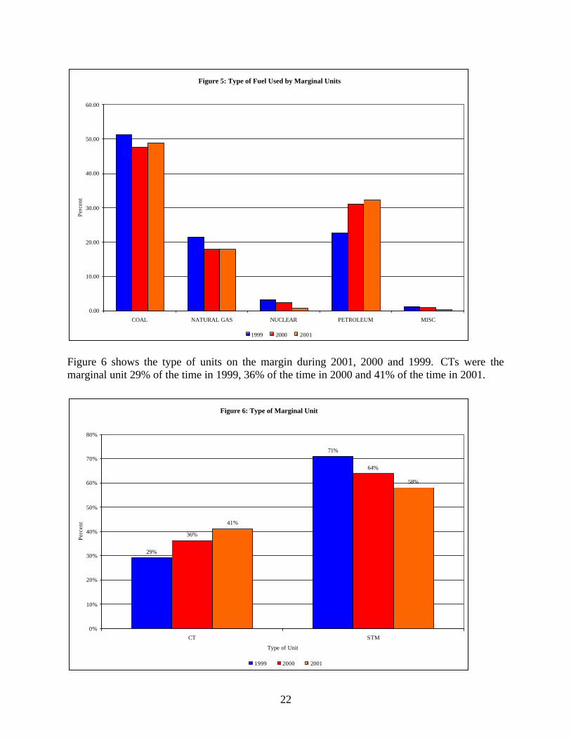
Figure 5 shows the type of fuel used by the marginal units. In 2001, coal-fired units were on themargin 49% of the time, petroleum-fired units 32% of the time, gas-fired units 18% of the timeand nuclear units 1%. Petroleum-fired units’ share of marginal usage increased from 31% in2000 to 32% in 2001, the share of coal also increased by about 1%, the shares of nuclear andmiscellaneous decreased and the share of natural gas was unchanged.

Figure 4: Average Mark Up Index by Type of Fuel

0.01 0.00 0.00

0.04

0.00

0.07

0.010.00

0.04

0.07

0.10

0.020.00

0.06

0.09

-0.1

0

0.1

0.2

0.3

0.4

0.5

COAL NATURAL GAS NUCLEAR PETROLEUM MISC

Inde

x

1999 2000 2001

22

Figure 6 shows the type of units on the margin during 2001, 2000 and 1999. CTs were themarginal unit 29% of the time in 1999, 36% of the time in 2000 and 41% of the time in 2001.

Figure 5: Type of Fuel Used by Marginal Units

0.00

10.00

20.00

30.00

40.00

50.00

60.00

COAL NATURAL GAS NUCLEAR PETROLEUM MISC

Perc

ent

1999 2000 2001

Figure 6: Type of Marginal Unit

29%

71%

36%

64%

41%

58%

0%

10%

20%

30%

40%

50%

60%

70%

80%

CT STM

Type of Unit

Perc

ent

1999 2000 2001

23

Steam units were the marginal unit 71% of the time in 1999, 64% of the time in 2000 and 58% ofthe time in 2001.

Figure 7 shows the average markup index by type of unit. The average annual mark up index washigher for steam units than for CTs, and the average annual index increased for both steam unitsand CTs in 2001.

Figure 8 shows the distribution of ownership of the marginal units. Taking all the units whichwere on the margin for one or more five-minute intervals during the year, in 2001, the bars onthe graph show that two companies each owned 15-20% of the marginal units while two othercompanies each owned 10-15% of the marginal units. The “2001 Total” line on the graph showsthat two companies owned the marginal unit in more than 30 percent of the five minute intervalsin 2001, while four companies owned the marginal unit in about 60 percent of the intervals in2001, and eight companies owned the marginal unit in almost 90 percent of the intervals. In2000, almost 80% of the marginal units were owned by the top five companies while in 1999,more than 60% of the marginal units were owned by the top five companies. When combinedwith the information on bidding behavior, the distribution of ownership of marginal units is afurther cause for concern.

Figure 7: Average Index by Type of Unit

0.03

0.010.02

0.06

0.03

0.09

0

0.05

0.1

0.15

0.2

0.25

CT STM

Inde

x

1999 2000 2001

24

Overall, the index results presented here are consistent with the conclusion that the energymarket was reasonably competitive in 2001. The MMU will continue to develop this analysis torefine the measure of the markup over competitive prices and to incorporate explicit accountingfor opportunity costs and scarcity rents.

Figure 8: Marginal Unit Ownership

0

2

4

6

8

10

12

14

16

5% or Less 10% 15% 20%

Percent of Marginal Units Owned by Individual Companies

Num

ber

of C

ompa

nies

0

10

20

30

40

50

60

Tot

al P

erce

nt o

f M

argi

nal U

nits

1999 2000 2001 2001 Total 2000 Total 1999 Total

25

Market StructureConcentration ratios are a summary measure of market shares, a key element of market structure.High concentration ratios mean that a small number of sellers dominate the market while lowconcentration ratios mean that a larger number of sellers share in market sales more equally.Concentration measures must be used carefully in assessing the competitiveness of markets. Thebest tests for assessing the competitiveness of markets are direct tests of the conduct andperformance of individual participants within markets and their impact on market prices. Theprice-cost markup test is one such test and direct examination of the offer behavior of individualmarket participants is another. Low aggregate- market concentration ratios do not establish that amarket is competitive or that market participants cannot exercise market power. However, highmarket concentration ratios do indicate an increased potential for market participants to exercisemarket power. Concentration ratios are presented here because they provide useful informationon market structure and are a widely used measure of market structure.

The analysis indicates that the PJM Control Area exhibits moderate energy market concentrationoverall, but that concentration in the intermediate and peaking segments of the supply curve ishigh. High levels of concentration, particularly in the peaking segment, increase the probabilitythat a generation owner will be pivotal during high demand periods. In addition, specific areas ofthe PJM system exhibit moderate to high market concentration that may be problematic whentransmission constraints exist. There is no evidence that market power was exercised in theseareas in 2001, primarily due to the load obligations of the generators in those areas, but asignificant market-power related risk exists going forward should those load obligations change.

MethodThe concentration ratio used here is the Herfindahl-Hirschman Index (HHI), calculated as thesum of the squares of the market shares of the firms in a market. Hourly energy market HHIswere calculated based on the real-time energy output of generators located in the PJM controlarea, adjusted for hourly imports (Table 2). The installed HHIs were calculated based on theinstalled capacity of PJM generating resources, adjusted for aggregate import capability (Table3). The ability of the transmission system to deliver external energy into the control area wasincorporated in the HHI calculations because additional energy can be imported into PJM undermost conditions. The overall maximum hourly HHI was calculated by assigning all actualpositive net tie flows in each hour to the market participant with the largest market share, whilethe overall minimum hourly HHI was determined by assigning hourly net tie flows to five non-affiliated market participants. The overall maximum installed HHI was calculated by assigningall import capability to the market participant with the largest market share, the overall minimuminstalled HHI was determined by assigning import capability to five non-affiliated marketparticipants and the overall average is the average of the two. For both hourly and installedHHIs, generators were aggregated by ownership and, in the case of affiliated companies, parentorganization. Hourly and installed HHIs were also calculated for baseload, intermediate andpeaking segments of generation supply. The hourly segment HHIs were calculated based onhourly market shares, unadjusted for imports, while the installed segment HHIs were calculatedon an installed capacity basis, also unadjusted for import capability.

26

In addition to the aggregate PJM calculations, HHIs were calculated for various areas of PJM toprovide an indication of the level of concentration that exists when specific areas within PJM areisolated from the larger PJM market by the existence of transmission constraints.

FERC’s Merger Policy Statement states that a market can be broadly characterized asunconcentrated when the market HHI is below 1000 (the equivalent of 10 firms with equalmarket shares), as moderately concentrated when the market HHI is between 1000 and 1800 andhighly concentrated when the market HHI is greater than 1800 (the equivalent of between 5 and6 firms with equal market shares).6

ResultsThe results of the aggregate PJM HHI calculations for both the installed and the hourly measure(Tables 2 and 3) indicate that the PJM energy market is, in general, moderately concentrated bythe FERC standards. Overall market concentration varies from 975 to 2140 based on the hourlymeasure and from 1155 to 1405 based on the installed measure.7

Table 2. 2001 PJM Hourly HHIsOverall

MinimumOverall

MaximumMaximum 1885 2140Average 1375 1565Minimum 975 1275

Table 3. 2001 PJM Installed HHIsOverall

MinimumOverall

AverageOverall

MaximumOverall 1155 1280 1405

Tables 4 and 5 include HHI values for the capacity and energy measures by supply curvesegment, including base load, intermediate and peaking plants. The hourly measure indicates thatintermediate and peaking segments are highly concentrated on average while the installedmeasure indicates that all segments are moderately concentrated on average. For both hourly andinstalled measures, HHIs are calculated for facilities located in PJM only.

Table 4. 2001 PJM Hourly HHIs by SegmentBase Intermediate Peak

Maximum 1725 4575 9080Average 1525 2925 5140Minimum 1325 1270 1200

6 77 FERC ¶ 61,263, Inquiry Concerning the Commission’s Merger Policy Under the Federal Power Act:

Policy Statement, Order No. 592, pages 64-70.7 The maximum HHI level for the Overall Maximum hourly measure is based on the assumption that all

imports are controlled by the market participant with the largest market share. While this is an importantsensitivity, there is no evidence that this has occurred or is likely to occur.

27

Table 5. 2001 PJM Installed HHIs by SegmentBase Intermediate Peak

HHI 1397 1448 1776

Figure 9 shows the HHI results for the Overall Minimum hourly measure.

High Market Concentration and Frequent CongestionThere were five areas within the PJM Control Area that had high local market concentration andexperienced frequent congestion in 2001: Northern Public Service, Northcentral Public Service,Eastern PJM, the Delmarva Peninsula, and the Atlantic subarea of Conectiv.

Northern Public Service was constrained during 602 hours in 2001, compared to 637 hours in2000. Of the congested hours, 45 percent occurred during on-peak periods. Energy transfers intothe area were primarily restricted by limitations on the Roseland-Cedar Grove and Cedar Grove-Clifton corridors. When this area is constrained, some 3,200-4,600 MW of load is isolated,depending on load levels. Market concentration for the local market is high, with a minimumHHI of 4800.

Northcentral Public Service also exhibits relatively high concentration and experienced localcongestion during 371 hours in 2001, a decrease of about 100 hours from 2000, with 80 percentof congested hours during on-peak periods. Energy transfers into the area were primarilyrestricted by limitations on the Brunswick-Edison-Meadow Road 138 kV circuit. When this area

Figure 9: 2001 PJM Hourly Energy Market Minimum HHI

0

500

1000

1500

2000

2500

Jan-01 Feb-01 Mar-01 Apr-01 May-01 Jun-01 Jul-01 Aug-01 Sep-01 Oct-01 Nov-01 Dec-01

28

is constrained, some 350-550 MW of load is isolated. Market concentration varies from aminimum HHI of 2200 to a maximum HHI of over 9000.

Transfers into PJM East were constrained by the Eastern Interface limit during 230 hours in2001, a decrease from 345 hours from 2000. Of the congested hours, 80 percent occurred duringon-peak periods. This constraint isolates 19-27,000 of eastern load from the rest of PJM. Marketconcentration was moderate to high with minimum, average, and maximum HHIs of 1695, 2270,and 2845. About 60 percent of the new generation projects in the PJM queues are located in theeastern region of PJM, which, if built, may decrease concentration and could reduce thefrequency of congestion.

Transmission reinforcements8 appear to have alleviated a major constraint that frequentlyaffected the entire Delmarva Peninsula. Prior to 2001, the DPL South voltage limit hadfrequently isolated some 1,100-1,850 MW of load on the peninsula. This constraint, which wasin effect during 229 hours in 2000, was not encountered at all during 2001. However, many localconstraints that typically isolate small, highly concentrated load pockets still exist and arefrequently encountered. Such local constraints occurred during more than 3,000 hours in 2000and nearly 2,000 hours in 2001, with 85% of congested hours occurring during on-peak periods.The HHIs in these areas ranged from 3500 to 10000. Twelve 69 kV and six 138 kV constraintswere encountered on the Peninsula during 2001.

The Atlantic Electric area also had many local constraints that typically isolated small, highlyconcentrated load pockets of 100 MW or less. Such constraints were in effect for 1,600 hoursduring 2001, an 1,100-hour increase over 2000, with 65 percent of the constraints occurringduring on-peak periods. Two 69 kV constraints accounted for 55 percent of the congested hours:Motts Farm-Cedar and Shield Alloy-Vineland. The HHIs in these load pockets were high,ranging from 3500 to 10000.

8 DPL transmission reinforcements:• Added 515 MVAR of capacitors (218 MVAR transmission, 297 MVAR distribution).• Added 300 MVAR of SVCs (150 MVAR at Indian River 230, 150 MVAR at Nelson 138).• Added a second Steele 230/138 transformer (increased capability by 289 MW).• Replaced Vienna 230/138 transformer (increased capability by 284 MW).• Converted Loretto-Oak Hall 69 kV to 138 kV (increased capability by 125 MW).• Added a second Oak Hall 138/69 transformer (increased capability by 134 MW).• Added a New Church 138 kV substation.• Added a second New Church-Oak Hall 138 kV (increased capability by 342 MW).

29

Energy Market PricesThe conduct of individual market entities within a market structure is reflected in market prices.The overall level of prices is a good general indicator of market performance, although overallprice results must be interpreted carefully because of the multiple factors that affect them. Theremainder of this section discusses PJM energy market prices. The Appendix providesmethodological background and additional, more detailed, price data and comparisons.

Prices in the Real-Time Spot MarketPrices are a key outcome of markets. Prices vary across hours, across days and across years, andprices vary for multiple reasons. Prices are an indicator of the level of competition in a market,although prices are not always easy to interpret. In a competitive market in long run equilibrium,prices are directly related to the cost of the marginal unit required to serve load. The mark upindex is a direct measure of that relationship. Prices in PJM, LMPs, are a broader indicator of thelevel of competition. While PJM has experienced price spikes, these have been limited induration and, in general, prices in PJM have been well below the marginal cost of the highestcost unit installed on the system. The pattern of prices within days and across months and yearsillustrates how prices are directly related to demand conditions and thus illustrates the potentialsignificance of price elasticity of demand in affecting price.

PJM average prices increased in 2001 over 2000 for several reasons including increased fuelcosts and relatively short periods of high load conditions. The simple hourly average system-wide LMP was 15.1% higher in 2001 than in 2000, $32.38/MWh versus $28.14/MWh and14.3% higher than in 1999.1 (Table 3.) When hourly load levels are reflected, the load-weightedLMP of $36.65/MWh in 2001 was 19.3% higher than in 2000 and 7.6% higher than in 1999.(Table 5.) The load-weighted result reflects the fact that market participants typically purchasemore energy during high price periods. However, when increased fuel costs are accounted for,the average fuel cost adjusted, load-weighted LMP in 2001 was 7.6% higher than in 2000,$33.05/MWh compared to $30.72/MWh. (Table 6.) Thus, after accounting for both the actualpattern of loads and the increased costs of fuel, average prices in PJM were 7.6% higher in 2001than in 2000.

Prices rose to their highest levels of the year during the week of August 6, 2001 when new levelsof peak demand were established on three successive days. During 2001, PJM average pricesexceeded $900/MWH for 10 hours and exceeded $150/MWH for 60 hours. While prices duringmost hours reflected the interaction of demand and lower-price energy offers, prices on high loaddays reflected a combination of market power and scarcity. Prices reflected economic scarcitybecause loads exceeded the energy available from units operating within PJM at prices equal tomarginal costs. Prices reflected market power because a significant block of MW offered theirenergy at prices exceeding marginal cost and exceeding the price of available imports. Theinteraction of high levels of demand and the supply offers from this high-priced block resulted inhigher prices. Competition from imports responding to these prices limited the duration of highprices. If the impact of prices during the high load week of August 6 were excluded, the averageload-weighted, fuel cost adjusted price would have been $29.98, a 5.7% decrease from 2000.

1 The simple average system-wide LMP is the average of the hourly LMP in each hour without any

weighting.

30

Energy market price levels are consistent with the conclusion that the energy market wasreasonably competitive in 2001.

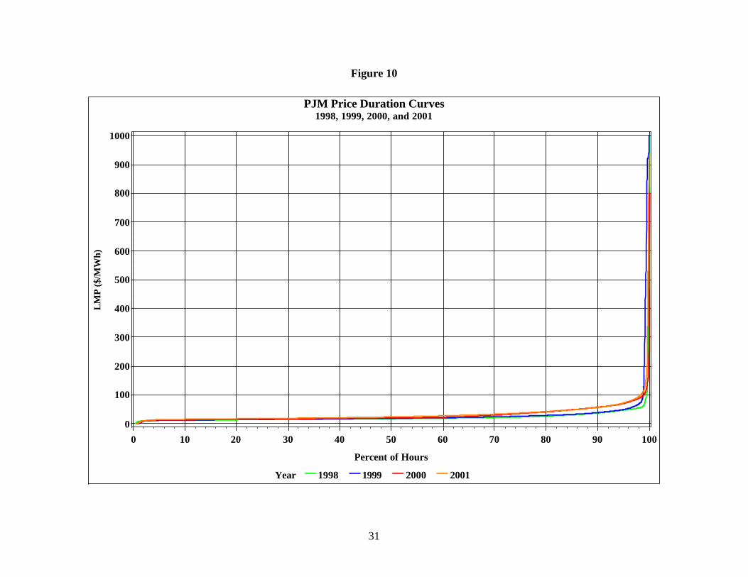
Figure 10 compares the PJM system-wide price duration curves for 1998, 1999, 2000, and 2001.A price duration curve represents the percent of hours that LMP was at or below a given price forthe year. Figure 10 shows that there was relatively little difference in LMPs for 60% of the hoursin each of the four years, for 96% of the hours in 2000 and 2001, and for more than 96% of thehours in 1998 and 1999. Figure 11 compares the price duration curves for hours above the 95th

percentile. Figure 11 shows that prices greater than $150/MWh occurred in each year for about1% or less of the hours.

As can be seen in Figures 10 and 11, LMPs exceeded $900/MWh in 1998, 1999, and 2001. In1998 and 1999, the highest prices occurred during the hot, summer months. Prices were above$900/MWh for a total of 35 hours during these two summers. In 2001, the highest LMPsoccurred during a single period of hot weather in the week of August 6, when new system peakloads occurred on three consecutive days, August 7, 8 and 9. During these three days, pricesexceeded $900/MWh for 10 hours. As a result of relatively mild weather, LMPs in 2000 did notreach the levels obtained in the other years, and did not exhibit the same volatility.

31

Figure 10

PJM Price Duration Curves1998, 1999, 2000, and 2001

Year 1998 1999 2000 2001

LM

P ($

/MW

h)

0

100

200

300

400

500

600

700

800

900

1000

Percent of Hours

0 10 20 30 40 50 60 70 80 90 100

32

Figure 11

PJM Price Duration CurvesHours Above the 95th Percentile

Year 1998 1999 2000 2001

LM

P ($

/MW

h)

0

100

200

300

400

500

600

700

800

900

1000

Percent of Hours

95 96 97 98 99 100

33

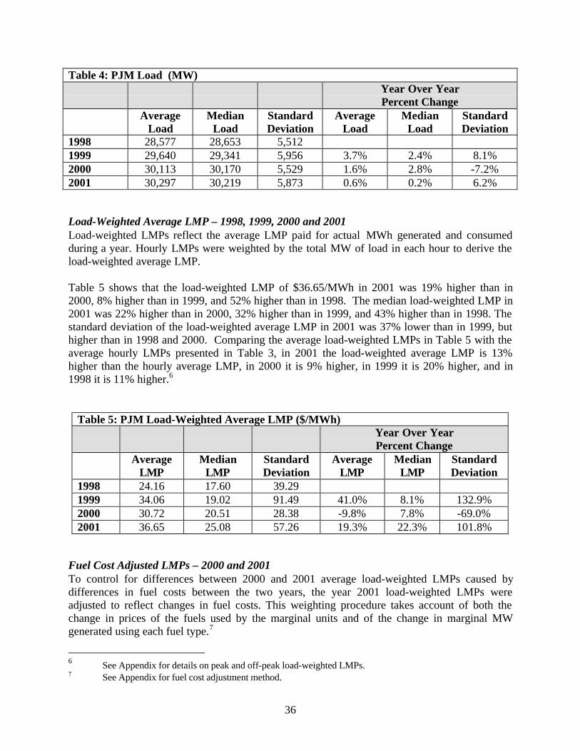
Table 3 provides summary LMP statistics for the years from 1998 to 2001. The annual statisticswere calculated from the hourly-integrated PJM system-wide LMPs (and MCPs for January –March 1998).2 Average system-wide LMP was about 15% higher in 2001 than 2000. Themedian3 LMP was more than 20% higher in 2001 than in 2000, 29% higher than in 1999, and38% higher than 1998. The standard deviation4 of average LMP is lowest in 2000 relative to theother years, reflecting the hotter summers in 1998, 1999, and 2001.

Table 3: PJM Average Hourly LMP ($/MWh)Year Over YearPercent Change

AverageLMP

MedianLMP

StandardDeviation

AverageLMP

MedianLMP

StandardDeviation

1998 21.72 16.60 31.451999 28.32 17.88 72.41 30.4% 7.7% 130.2%2000 28.14 19.11 25.69 -0.6% 6.9% -64.5%2001 32.38 22.98 45.03 15.1% 20.3% 75.3%

Load – 1998, 1999, 2000 and 2001Figure 12 shows the load duration curve for the years 1998, 1999, 2000 and 2001. Figure 12indicates that load in 2001 was virtually identical to load in 2000 for slightly more than 90% ofthe hours, with load in 2001 reaching higher levels for about 10% of the hours due in part to thehot week of August 6. Indeed, new peak demand was set on three consecutive days during thisweek, surpassing the previous peak demand of 51,700 MW established in July 1999. On August7 a new peak demand of 53,071 MW was established; on August 8 a new peak demand of 53,531MW was established; and on August 9 the final new peak demand of 54,014 MW wasestablished.

Table 4 presents summary load statistics for the four years. The average load of 30,297 MW in2001 was 0.6% higher than in 2000, 2.2% higher than in 1999, and 6% higher than in 1998. Themedian load in 2001 was also 0.2% higher than in 2000. The variability in load, indicated by thestandard deviation, increased by 6.2% in 2001.5

2 MCP is the single market clearing price calculated by PJM prior to implementation of LMP.3 The median is defined as the midpoint of the data values. Fifty percent of the data values lie above the

median and fifty percent lie below the median.4 The standard deviation is a measure of the variability of the data around the mean. 68% of the data will lie

within plus and minus one standard deviation from the mean.5 See Appendix for more details on load frequency including on-peak and off-peak loads.

35

Figure 12

PJM Hourly Load Duration Curve1998, 1999, 2000, and 2001

Year 1998 1999 2000 2001

PJM

Loa

d (M

W)

10000

20000

30000

40000

50000

60000

Percent of Hours

0 10 20 30 40 50 60 70 80 90 100

36

Table 4: PJM Load (MW)Year Over YearPercent Change

AverageLoad

MedianLoad

StandardDeviation

AverageLoad

MedianLoad

StandardDeviation

1998 28,577 28,653 5,5121999 29,640 29,341 5,956 3.7% 2.4% 8.1%2000 30,113 30,170 5,529 1.6% 2.8% -7.2%2001 30,297 30,219 5,873 0.6% 0.2% 6.2%

Load-Weighted Average LMP – 1998, 1999, 2000 and 2001Load-weighted LMPs reflect the average LMP paid for actual MWh generated and consumedduring a year. Hourly LMPs were weighted by the total MW of load in each hour to derive theload-weighted average LMP.

Table 5 shows that the load-weighted LMP of $36.65/MWh in 2001 was 19% higher than in2000, 8% higher than in 1999, and 52% higher than in 1998. The median load-weighted LMP in2001 was 22% higher than in 2000, 32% higher than in 1999, and 43% higher than in 1998. Thestandard deviation of the load-weighted average LMP in 2001 was 37% lower than in 1999, buthigher than in 1998 and 2000. Comparing the average load-weighted LMPs in Table 5 with theaverage hourly LMPs presented in Table 3, in 2001 the load-weighted average LMP is 13%higher than the hourly average LMP, in 2000 it is 9% higher, in 1999 it is 20% higher, and in1998 it is 11% higher.6

Table 5: PJM Load-Weighted Average LMP ($/MWh)Year Over YearPercent Change

AverageLMP

MedianLMP

StandardDeviation

AverageLMP

MedianLMP

StandardDeviation

1998 24.16 17.60 39.291999 34.06 19.02 91.49 41.0% 8.1% 132.9%2000 30.72 20.51 28.38 -9.8% 7.8% -69.0%2001 36.65 25.08 57.26 19.3% 22.3% 101.8%

Fuel Cost Adjusted LMPs – 2000 and 2001To control for differences between 2000 and 2001 average load-weighted LMPs caused bydifferences in fuel costs between the two years, the year 2001 load-weighted LMPs wereadjusted to reflect changes in fuel costs. This weighting procedure takes account of both thechange in prices of the fuels used by the marginal units and of the change in marginal MWgenerated using each fuel type.7

6 See Appendix for details on peak and off-peak load-weighted LMPs.7 See Appendix for fuel cost adjustment method.

37

Table 6 compares 2001 load-weighted, fuel cost adjusted average LMPs to 2000 load-weightedaverage LMPs. The table shows that after adjusting for fuel price changes between the two years,average load-weighted LMP in 2001 was 7.6% higher than in 2000, $33.05/MWh compared to$30.72/MWh. Thus, if fuel prices had been the same in 2001 as in 2000, the 2001 load-weightedLMP would have been about 10% lower, $33.05/MWh instead of $36.65/MWh, or an 8%increase over 2000.8 In other words, more than half the 19% increase in the load-weighted LMPbetween 2000 and 2001 was the result of increased fuel costs. The increase in the median load-weighted, fuel cost adjusted LMP was 14.5%, $23.49/MWh in 2001 to $20.51/MWh in 2000.The standard deviation of load-weighted, fuel cost adjusted LMP was 95% higher in 2001 than2000.

Table 6: Load-Weighted, Fuel Cost Adjusted LMPs ($/MWh)2000 2001 % Increase

Average LMP 30.72 33.05 7.6%Median LMP 20.51 23.49 14.5%Standard Deviation 28.38 55.34 95.0%

Day-Ahead and Real-Time Market LMPsThe day-ahead market was introduced on June 1, 2000. The day-ahead and real-time marketcomparisons that follow are for calendar year 2001. It would be expected that competition wouldcause the prices in the day-ahead and real-time markets to tend to converge. On average, day-ahead prices were slightly greater than real-time prices during 2001. Figure 13 shows the priceduration curve for the two markets, while Figure 14 shows the price duration curve for hoursabove the 95th percentile. Real-time prices are slightly lower than day-ahead prices for the lowestpriced 80% of the hours and are higher for the remaining 20% of the hours while the differenceincreases in the highest priced 1% or less of the hours. This difference reflects in part the pricelevels in real time during the hot week of August 6, which were not fully anticipated in the day-ahead market. Figure 15 compares average day-ahead and real-time LMPs for each hour. Figure16 shows the difference between real-time hourly LMP and day-ahead hourly LMP (real-timeLMP minus day-ahead LMP).9

8 See Appendix for details on LMPs during constrained hours.9 See Appendix for more details on the frequency distribution of prices.

38

Figure 13

PJM Price Duration CurvesReal Time and Day Ahead Markets - 2001

Market Day Ahead Real Time

LM

P ($

/MW

h)

-100

0

100

200

300

400

500

600

700

800

900

1000

Percent of Hours

0 10 20 30 40 50 60 70 80 90 100

39

Figure 14

PJM Price Duration CurvesReal Time and Day Ahead Markets - 2001

Hours Above the 95th Percentile

Market Day Ahead Real Time

LM

P ($

/MW

h)

0

100

200

300

400

500

600

700

800

900

1000

Percent of Hours

95 96 97 98 99 100

40

Figure 15

PJM Average Hourly System LMPDay Ahead and Real Time Markets

2001

Market Day Ahead Real Time

LM

P ($

/MW

h)

10

20

30

40

50

Hour

1 2 3 4 5 6 7 8 9 10 11 12 13 14 15 16 17 18 19 20 21 22 23 24

41

Figure 16

Hourly RT LMP Minus DA LMP2001

LM

P D

iffe

renc

e ($

/MW

h)

-500

-400

-300

-200

-100

0

100

200

300

400

500

600

700

Hour

01/01/01 03/01/01 05/01/01 07/01/01 09/01/01 11/01/01 01/01/02

42

Figure 16 shows that the difference between day-ahead and real-time prices narrowed during2001, excluding the week of August 6.

Table 7 presents summary statistics for the two markets. The average LMP in the day-aheadmarket was $0.37/MWh or 1.1% higher than the average LMP in the real-time market. The day-ahead median LMP was 17.7% larger than the real-time LMP, an average difference of$4.07/MWh. Consistent with the price duration curve, price dispersion in the real-time market is32.5% higher than the day-ahead market, with the average difference in standard deviationbetween the two markets of $14.61/MWh.10 11

Table 7: Comparison of Real-Time and Day-Ahead Market LMPs ($/MWh)

Day-Ahead Real-TimeAverage

DifferencePercent Over Real-

TimeAverage LMP 32.75 32.38 -0.37 1.1%Median LMP 27.05 22.98 -4.1 17.7%Standard Deviation 30.42 45.03 14.6 -32.5%

Day-Ahead and Real-Time Market Generation and LoadDay-Ahead and Real-Time GenerationThere are three types of “generation” in the day-ahead market – self-scheduled generation,generator offers, and increment offers. Self-scheduled generation can be submitted as a fixedblock of MW that must be run, or as a minimum amount of MW that must run plus adispatchable component above the minimum. Generator offers are schedules of MW offered andthe corresponding offer price. Finally, increment offers are financial offers in the day-aheadmarket to supply a specified amount of MW at, or above, a given price. In all cases,commitments made and cleared in the day-ahead market are financially binding. Real-timegeneration is the actual production of electricity during the operating day.

Figure 17 shows the average hourly values of day-ahead generation, day-ahead generation plusincrement offers, and real-time generation. Day-ahead generation is generation that is cleared inthe day-ahead market. Real-time generation is always higher than day-ahead generation.However, when increment offers are added to day-ahead generation, total day-ahead MW offersalways exceed real-time generation.

Table 8 presents summary statistics for day-ahead and real-time generation and the averagedifferences between the two. The table shows that real-time generation averaged 2,757 MWmore than day-ahead generation.

10 See Appendix for more details on peak and off-peak LMPs.11 See Appendix for more details on LMPs during constrained hours.

43

Figure 17

Real Time and Day Ahead Generation2001

Average Hourly Values

DA_GEN RT_GEN DA_GEN_plus_INCS

MW

21000

22000

23000

24000

25000

26000

27000

28000

29000

30000

31000

32000

33000

34000

35000

36000

37000

38000

Hour Ending

1 2 3 4 5 6 7 8 9 10 11 12 13 14 15 16 17 18 19 20 21 22 23 24

44

When increment offers are added to day-ahead generation offers, the sum in the day-aheadmarket is 3,790 MW higher than real-time generation.

Table 8: Day-Ahead and Real-Time Generation (MW)Day-Ahead Real-Time Average Difference

GenerationIncrement

Offers Generation Generation

DA GenerationPlus Increment

OffersAverage MW 26,423 6,547 29,180 2,757 3,790Median MW 26,002 6,284 28,977 2,715 3,549StandardDeviation 4,767 2,172 5,315

As can be seen in Figure 17, the differences among the three types of day-ahead generationoffers widen during peak hours (hours ending 8 to 23). Table 9 shows the average MW values inthe day-ahead and real-time markets during the off-peak and peak hours, while Table 10 showsthe average differences during the two periods. Real-time generation exceeds day-aheadgeneration during both periods. The average difference between real-time and day-aheadgeneration during off- peak hours is 2,216 MW, and the average difference during peak hours is

Table 9: Day-Ahead and Real-Time Peak and Off-Peak Generation (MW)Day-Ahead Real-Time

Off-Peak Peak Off-Peak Peak Off-Peak Peak

Generation GenerationIncrement

OffersIncrement

Offers Generation GenerationAverageMW 23,897 29,320 5,199 8,094 26,114 32,697MedianMW 23,481 28,183 5,045 7,824 25,685 31,549StandardDeviation 3,620 4,248 1,339 1,894 3,925 4,453

3,377 MW. When increment offers are added to day-ahead generation, the total exceeds real-time generation during both periods. During off-peak hours, day-ahead generation plusincrement offers averaged 2,982 MW more than real-time generation, and during peak hours,day-ahead generation plus increment offers averaged 4,716 MW more than real-time generation.

45

Table 10: Average Differences Between Day-Ahead and Real-Time Markets (MW)Off-Peak Peak

GenerationGeneration Plus

Increment Offers GenerationGeneration Plus

Increment OffersAverage MW

Difference 2,216 2,982 3,377 4,716Median MWDifference 2,211 2,904 3,415 4,626

Day-Ahead and Real-Time LoadThere are three types of load in the day-ahead market. Fixed demand bids represent load that willpurchase a defined MW level of energy, regardless of the level of LMP. Price sensitive bidsrepresent load that will purchase a defined MW level of energy only up to a specified LMP;above that LMP, the load bid is zero. Decrement bids are similar to price sensitive bids in thatthey represent load that will purchase a defined MW level of energy up to a specified LMP andare zero above that LMP. However, decrement bids are financial bids that can be submitted byany market participant. All load bids that are cleared in the day-ahead market are financiallybinding. Real-time load is the actual load on the system during the operating day.

Figure 18 shows the average hourly values of day-ahead fixed demand, price sensitive load,decrement bids, and total day-ahead and real-time load (total day-ahead load is defined here asthe sum of the three demand components). Table 11 presents the summary statistics for the day-ahead load components, total day-ahead load, real-time load, and the average difference betweentotal day-ahead load and total real-time load. As Figure 18 and Table 11 show, total day-aheadload was higher than real-time load by an average of 3,026 MW. The table also shows that fixeddemand is the largest component of day-ahead load, 77%, while price sensitive was the smallestcomponent, 7%, with decrement bids accounting for the remaining 16% of day-ahead load.

Table 11: Day-Ahead and Real-Time Load (MW)Day-Ahead Real-Time

FixedDemand

PriceSensitive

DecrementBids

Total DALoad

Total RTLoad

AverageDifference

AverageMW 25,741 2,195 5,383 33,318 30,297 3,026MedianMW 25,420 2,144 5,159 32,812 30,219 2,983StandardDeviation 5,234 640 1,403 6,489 5,873

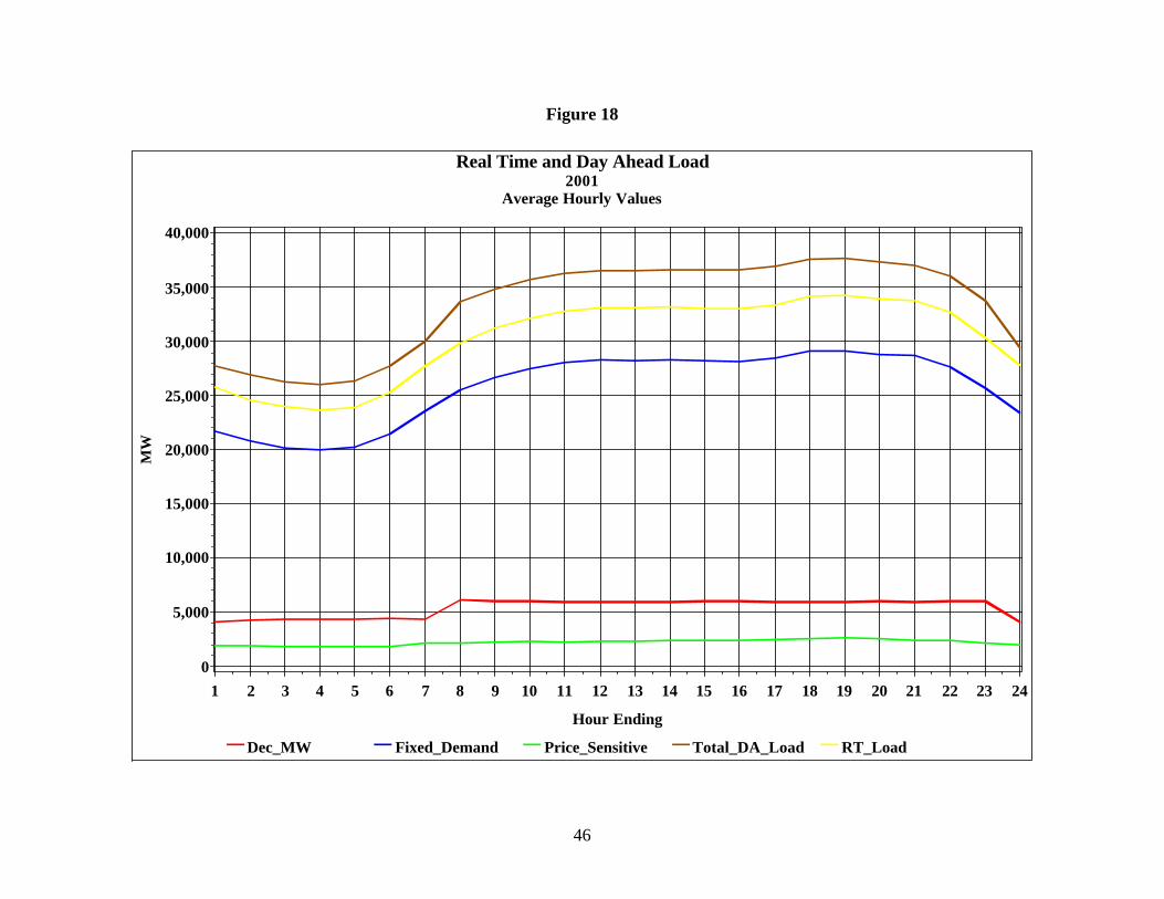
46

Figure 18

Real Time and Day Ahead Load2001

Average Hourly Values

Dec_MW Fixed_Demand Price_Sensitive Total_DA_Load RT_Load

MW

0

5,000

10,000

15,000

20,000

25,000

30,000

35,000

40,000

Hour Ending

1 2 3 4 5 6 7 8 9 10 11 12 13 14 15 16 17 18 19 20 21 22 23 24

47

As can be seen in Figure 18, the day-ahead load components (except for price sensitive demand)increased during the peak hours (hours ending 8 to 23), as did real-time load. Table 12 shows theaverage load MW values in the day-ahead and real-time markets during the off-peak and peakhours. Total day-ahead load was higher than real time load during both off-peak and peak hours.The average difference during off-peak hours was 2,483 MW, while the average differenceduring peak hours was 3,636 MW. The percentage of day-ahead load comprised by each of thecomponents is similar during the two periods. Fixed demand accounts for the largest percentageof day-ahead load during the off-peak and peak periods, 77% during both periods, with pricesensitive load accounting for the smallest percentage during both periods, 7% and 6%,respectively, and decrement bids accounting for 16% and 17%, respectively.

Table 12: Day-Ahead and Real-Time Load During Off-Peak and Peak Hours (MW)Day-Ahead Real-Time

Off-Peak PeakOff-Peak Peak

FixedDemand

PriceSensitive

DecrementBids

TotalLoad

FixedDemand

PriceSensitive

DecBids

TotalLoad

TotalLoad

TotalLoad

AverageMW 22,629 2,074 4,584 29,287 29,307 2,334 6,298 37,939 26,804 34,303MedianMW 22,235 1,983 4,573 28,854 28,313 2,352 6,201 36,864 26,433 33,076StandardDeviation 3,692 603 902 4,322 4,400 652 1,311 5,383 4,225 4,851

Figure 19 shows day-ahead and real-time load and generation. Note that increment offers havebeen subtracted from total day-ahead load. Since increment offers look like generation,subtracting increment offers from day-ahead load provides an estimate of day-ahead generationthat must be turned on to meet the load.

Another difference between the two markets is the lower level of net external transactions(imports and exports) in the day-ahead market. In the real-time market, during peak hours, nettransactions averaged 1,606 MW. During the same period in the day-ahead market, nettransactions averaged 525 MW. A final observation is that there is a relatively constantdifference between real-time load and day-ahead load excluding decrement bids; that is, day-ahead load as fixed plus price sensitive load. During off-peak hours the difference between real-time load and fixed plus price sensitive load averages 2,101 MW, while during peak hours theaverage difference is 2,662 MW.

48

Figure 19

Real Time and Day Ahead Load and Generation2001

Average Hourly Values

DA_Load_minus_Incs Fixed_plus_Price_Sensitive DA_GenRT_Gen RT_Load

MW

21,000

22,000

23,000

24,000

25,000

26,000

27,000

28,000

29,000

30,000

31,000

32,000

33,000

34,000

35,000

Hour Ending

1 2 3 4 5 6 7 8 9 10 11 12 13 14 15 16 17 18 19 20 21 22 23 24

49

AppendixFrequency Distribution of LMPFigures A.1, A.2, A.3, and A.4 provide the frequency distribution, by hour, of LMPs for 1998,1999, 2000 and 2001.12 The figures show the number of hours (FREQ.), the cumulative numberof hours (CUM FREQ.), the percent of hours (PCT.), and the cumulative percent of hours (CUMPCT.) that LMPs were within a given $10 price interval.13

Comparing the figures, it can be seen that LMPs were most frequently in the interval $10/MWhto $20/MWh in each year. However, a decreasing percentage of hours fell in this interval in eachsucceeding year: 65% in 1998; 58% in 1999; 51% in 2000; and 36% in 2001. In 1998, 1999,2000, and 2001, prices were less than $30/MWh 85%, 83%, 71%, and 66% of the hours,respectively. LMPs were less than $60/MWh 99%, 97%, 92%, and 92% of the hours,respectively, and less than $100/MWh 99.4%, 98.8%, 98.9%, and 98.4% of the hours,respectively. LMP was $150/MWh or greater for 60 hours (0.7% of the hours) in 2001, 27 hours(0.3% of the hours) in 2000, 95 hours (1% of the hours) in 1999, and 29 hours (0.3% of thehours) in 1998.

Frequency Distribution of LoadFigures A.5, A.6, A.7, and A.8 provide the frequency distribution, by hour, of LMPs for 1998,1999, 2000 and 2001. The figures show that in 1998 and 1999 load was most frequently in therange of 25,000 to 30,000 MW, 35% and 34% of the hours, respectively, and that load was lessthan 30,000 MW for 63% of the hours in 1998 and 56% of the hours in 1999. By contrast, loadwas most frequently in the range of 30,000 to 35,000 MW in 2000 and 2001, 34% of the hours ineach year, and was less than 30,000 MW for 48% of the hours in each year. Load was less than45,000 MW for 99% of the hours in both 1998 and 2000, and never exceeded 50,000 MW. Loadwas less than 45,000 MW for 98% of the hours in both 1999 and 2001. Load in 1999 exceeded50,000 MW for 15 hours and for 53 hours in 2001. A new all-time peak demand was set in bothyears: 51,700 MW in 1999 and 54,014 in 2001.

On-Peak and Off-Peak LoadTable A.1 presents the summary load statistics for 1998 to 2001 for the off-peak and peak hours,while Table A.2 shows the percentage changes in load year to year. The peak period is definedfor each weekday (Monday through Friday) as hour ending 0800 to hour ending 2300, excludingholidays. As can be seen from the table, in all four years peak load is about 30% higher than theoff-peak load, while the median peak load ranges from 20% to 30% higher. Average load duringpeak hours in 2001 was about 1.6% higher than that in 2000, 3% higher than in 1999, and 6.1%higher than in 1998. Off-peak load in 2001 was 0.4% lower than in 2000, but higher than in1999 and 1998, 1.5% and 6.1%, respectively.

12 LMPs were instituted in PJM in April, 1998. Prior to April, there was a single system price, the Market

Clearing Price (MCP), which was the system lambda.13 Only LMP intervals with a positive frequency are included in the figure.

50

Figure A.1

Frequency Distribution by Hours of PJM LMPs - 1998

FREQ.CUM.

FREQ. PCT.CUM.PCT.

204 204 2.33 2.335729 5933 65.40 67.731539 7472 17.57 85.30

607 8079 6.93 92.23396 8475 4.52 96.75178 8653 2.03 98.78

27 8680 0.31 99.0910 8690 0.11 99.2015 8705 0.17 99.376 8711 0.07 99.44

11 8722 0.13 99.571 8723 0.01 99.581 8724 0.01 99.594 8728 0.05 99.633 8731 0.03 99.676 8737 0.07 99.742 8739 0.02 99.761 8740 0.01 99.771 8741 0.01 99.781 8742 0.01 99.791 8743 0.01 99.815 8748 0.06 99.862 8750 0.02 99.891 8751 0.01 99.901 8752 0.01 99.911 8753 0.01 99.921 8754 0.01 99.931 8755 0.01 99.943 8758 0.03 99.982 8760 0.02 100.00

LMP ($/MWh)

$990 to $1,000$890 to $900$850 to $860$700 to $710$680 to $690$510 to $520$500 to $510$460 to $470$300 to $310$240 to $250$220 to $230$200 to $210$190 to $200$180 to $190$150 to $160$140 to $150$130 to $140$120 to $130$110 to $120$100 to $110

$90 to $100$80 to $90$70 to $80$60 to $70$50 to $60$40 to $50$30 to $40$20 to $30$10 to $20$ 0 to $10

FREQUENCY (Hours)

0 1000 2000 3000 4000 5000 6000

51

Figure A.2

Frequency Distribution by Hours of PJM LMPs - 1999

FREQ.CUM.

FREQ. PCT.CUM.PCT.

227 227 2.59 2.595042 5269 57.56 60.151982 7251 22.63 82.77733 7984 8.37 91.14379 8363 4.33 95.47154 8517 1.76 97.2384 8601 0.96 98.1833 8634 0.38 98.5613 8647 0.15 98.718 8655 0.09 98.804 8659 0.05 98.853 8662 0.03 98.882 8664 0.02 98.901 8665 0.01 98.924 8669 0.05 98.961 8670 0.01 98.971 8671 0.01 98.981 8672 0.01 99.002 8674 0.02 99.022 8676 0.02 99.041 8677 0.01 99.051 8678 0.01 99.061 8679 0.01 99.081 8680 0.01 99.092 8682 0.02 99.112 8684 0.02 99.132 8686 0.02 99.161 8687 0.01 99.171 8688 0.01 99.181 8689 0.01 99.192 8691 0.02 99.211 8692 0.01 99.222 8694 0.02 99.251 8695 0.01 99.261 8696 0.01 99.273 8699 0.03 99.301 8700 0.01 99.321 8701 0.01 99.331 8702 0.01 99.342 8704 0.02 99.362 8706 0.02 99.381 8707 0.01 99.391 8708 0.01 99.411 8709 0.01 99.422 8711 0.02 99.441 8712 0.01 99.451 8713 0.01 99.462 8715 0.02 99.491 8716 0.01 99.501 8717 0.01 99.511 8718 0.01 99.527 8725 0.08 99.601 8726 0.01 99.611 8727 0.01 99.621 8728 0.01 99.63

10 8738 0.11 99.7511 8749 0.13 99.872 8751 0.02 99.901 8752 0.01 99.911 8753 0.01 99.927 8760 0.08 100.00

LMP ($/MWh)

$990 to $1,000$970 to $980$950 to $960$940 to $950$930 to $940$910 to $920$900 to $910$890 to $900$870 to $880$840 to $850$820 to $830$790 to $800$780 to $790$760 to $770$750 to $760$670 to $680$620 to $630$610 to $620$600 to $610$570 to $580$560 to $570$540 to $550$530 to $540$510 to $520$490 to $500$470 to $480$460 to $470$450 to $460$440 to $450$430 to $440$400 to $410$370 to $380$360 to $370$330 to $340$310 to $320$300 to $310$270 to $280$260 to $270$250 to $260$240 to $250$220 to $230$200 to $210$190 to $200$180 to $190$170 to $180$160 to $170$140 to $150$130 to $140$120 to $130$110 to $120$100 to $110$90 to $100$80 to $90$70 to $80$60 to $70$50 to $60$40 to $50$30 to $40$20 to $30$10 to $20$ 0 to $10

FREQUENCY (Hours)

0 1000 2000 3000 4000 5000 6000

52

Figure A.3

Frequency Distribution by Hours of PJM LMPs - 2000

FREQ.CUM.

FREQ. PCT.CUM.PCT.

210 210 2.39 2.394522 4732 51.48 53.871494 6226 17.01 70.88

782 7008 8.90 79.78591 7599 6.73 86.51459 8058 5.23 91.73315 8373 3.59 95.32147 8520 1.67 96.99115 8635 1.31 98.30

56 8691 0.64 98.9431 8722 0.35 99.29

9 8731 0.10 99.4013 8744 0.15 99.54

5 8749 0.06 99.608 8757 0.09 99.696 8763 0.07 99.763 8766 0.03 99.802 8768 0.02 99.821 8769 0.01 99.832 8771 0.02 99.851 8772 0.01 99.861 8773 0.01 99.872 8775 0.02 99.901 8776 0.01 99.911 8777 0.01 99.921 8778 0.01 99.934 8782 0.05 99.981 8783 0.01 99.991 8784 0.01 100.00

LMP ($/MWh)

$800 to $810$590 to $600$480 to $490$360 to $370$290 to $300$280 to $290$260 to $270$220 to $230$210 to $220$190 to $200$180 to $190$170 to $180$160 to $170$150 to $160$140 to $150$130 to $140$120 to $130$110 to $120$100 to $110

$90 to $100$80 to $90$70 to $80$60 to $70$50 to $60$40 to $50$30 to $40$20 to $30$10 to $20$ 0 to $10

FREQUENCY (Hours)

0 1000 2000 3000 4000 5000

53

Figure A.4

Frequency Distribution by Hours of PJM LMPs - 2001

FREQ.CUM.

FREQ. PCT.CUM.PCT.

210 210 2.40 2.403167 3377 36.15 38.552423 5800 27.66 66.211109 6909 12.66 78.87

704 7613 8.04 86.91433 8046 4.94 91.85264 8310 3.01 94.86155 8465 1.77 96.63104 8569 1.19 97.82

50 8619 0.57 98.3936 8655 0.41 98.8018 8673 0.21 99.0113 8686 0.15 99.16

5 8691 0.06 99.219 8700 0.10 99.326 8706 0.07 99.386 8712 0.07 99.452 8714 0.02 99.475 8719 0.06 99.531 8720 0.01 99.541 8721 0.01 99.551 8722 0.01 99.571 8723 0.01 99.583 8726 0.03 99.611 8727 0.01 99.621 8728 0.01 99.631 8729 0.01 99.652 8731 0.02 99.671 8732 0.01 99.682 8734 0.02 99.701 8735 0.01 99.711 8736 0.01 99.731 8737 0.01 99.743 8740 0.03 99.771 8741 0.01 99.782 8743 0.02 99.811 8744 0.01 99.822 8746 0.02 99.841 8747 0.01 99.851 8748 0.01 99.861 8749 0.01 99.871 8750 0.01 99.893 8753 0.03 99.921 8754 0.01 99.931 8755 0.01 99.945 8760 0.06 100.00

LMP ($/MWh)

$930 to $940$920 to $930$910 to $920$900 to $910$830 to $840$770 to $780$740 to $750$690 to $700$650 to $660$620 to $630$550 to $560$530 to $540$520 to $530$470 to $480$440 to $450$390 to $400$370 to $380$360 to $370$330 to $340$320 to $330$290 to $300$280 to $290$260 to $270$250 to $260$240 to $250$210 to $220$190 to $200$180 to $190$170 to $180$160 to $170$150 to $160$140 to $150$130 to $140$120 to $130$110 to $120$100 to $110

$90 to $100$80 to $90$70 to $80$60 to $70$50 to $60$40 to $50$30 to $40$20 to $30$10 to $20$ 0 to $10

FREQUENCY (Hours)

0 1000 2000 3000 4000

54

Figure A.5

Frequency Distribution of Hourly PJM Load - 1998

FREQ.CUM.

FREQ. PCT.CUM.PCT.

356 356 4.06 4.06

2137 2493 24.39 28.46

3063 5556 34.97 63.42

2171 7727 24.78 88.21

704 8431 8.04 96.24

270 8701 3.08 99.33

59 8760 0.67 100.00

Load (MW)

45,000 to 50,000

40,000 to 45,000

35,000 to 40,000

30,000 to 35,000

25,000 to 30,000

20,000 to 25,000

20,000 and Less

FREQUENCY (Hours)

0 1000 2000 3000 4000

55

Figure A.6

Frequency Distribution of Hourly PJM Load - 1999

FREQ.CUM.

FREQ. PCT.CUM.PCT.

218 218 2.49 2.49

1776 1994 20.27 22.76

2944 4938 33.61 56.37

2476 7414 28.26 84.63

773 8187 8.82 93.46

392 8579 4.47 97.93

166 8745 1.89 99.83

15 8760 0.17 100.00

Load (MW)

50,000 to 55,000

45,000 to 50,000

40,000 to 45,000

35,000 to 40,000

30,000 to 35,000

25,000 to 30,000

20,000 to 25,000

20,000 and Less

FREQUENCY (Hours)

0 1000 2000 3000

56

Figure A.7

Frequency Distribution of Hourly PJM Load - 2000

FREQ.CUM.

FREQ. PCT.CUM.PCT.

99 99 1.13 1.13

1658 1757 18.88 20.00

2485 4242 28.29 48.29

2975 7217 33.87 82.16

1159 8376 13.19 95.36

337 8713 3.84 99.19

71 8784 0.81 100.00

Load (MW)

45,000 to 50,000

40,000 to 45,000

35,000 to 40,000

30,000 to 35,000

25,000 to 30,000

20,000 to 25,000

20,000 and Less

FREQUENCY (Hours)

0 1000 2000 3000

57

Figure A.8

Frequency Distribution of Hourly PJM Load - 2001

FREQ.CUM.

FREQ. PCT.CUM.PCT.

107 107 1.22 1.22

1597 1704 18.23 19.45

2502 4206 28.56 48.01

3032 7238 34.61 82.63

965 8203 11.02 93.64

376 8579 4.29 97.93

128 8707 1.46 99.39

53 8760 0.61 100.00

Load (MW)

50,000 to 55,000

45,000 to 50,000

40,000 to 45,000

35,000 to 40,000

30,000 to 35,000

25,000 to 30,000

20,000 to 25,000

20,000 and Less

FREQUENCY (Hours)

0 1000 2000 3000 4000

58

Table A.1: Off-Peak and Peak Load – 1998, 1999, 2000, and 2001 (MW)Average Load Median Load Standard Deviation

YearOff-Peak Peak

Peak/Off-Peak

Off-Peak Peak

Peak/Off-Peak

Off-Peak Peak

Peak/Off-Peak

1998 25,268 32,344 1.3 24,728 31,081 1.3 4,091 4,388 1.11999 26,409 33,291 1.3 25,795 31,987 1.2 4,862 4,870 1.02000 26,921 33,766 1.3 26,327 32,771 1.2 4,453 4,226 0.92001 26,804 34,303 1.3 26,433 33,076 1.3 4,225 4,851 1.1

Table A.2: Year Over Year Percent Change in LoadAverage Load Median Load Standard Deviation

Year Off-Peak Peak Off-Peak Peak Off-Peak Peak19981999 4.5% 2.9% 4.3% 2.9% 18.8% 11.0%2000 1.9% 1.4% 2.1% 2.5% -8.4% -13.2%2001 -0.4% 1.6% 1.4% 0.9% -5.1% 14.8%

Peak and Off-Peak Load-Weighted LMPs – 2000 and 2001Table A.3 shows the load-weighted average LMPs for 2000 and 2001 during the off-peak andpeak periods. In 2000 the peak load-weighted LMP was 80% greater than the off-peak LMP,while in 2001 it was about 110% greater. The peak load-weighted average LMP in 2001 was25% higher than in 2000, while the off-peak LMP in 2001 was 8% higher than in 2000. Both thepeak and off-peak median LMPs were higher in 2001 than in 2000, 10% and 16%, respectively.The dispersion in LMPs, as indicated by the standard deviation, was higher in 2001 during peakhours, 138% higher than 2000, while the standard deviation of off-peak LMPs showed a 33%reduction in 2001.

Contrasting Tables A.3 with Table 5, the average on-peak load-weighted LMP in 2001 was 32%higher than the all-hours load-weighted average, while the off-peak load-weighted average LMPwas 36% lower than the all-hours load-weighted average. Similarly, in 2000 the average on-peakload-weighted LMP was 26% higher than the all-hours load-weighted average, while the off-peak load-weighted average LMP was 29% lower than the all-hours load-weighted average.

Table A.3: Off-Peak and Peak Load-weighted LMPs – 2000 and 2001 ($/MWh)

2000 2001% Change

2000 to 2001Off-Peak Peak

Peak/Off-Peak

Off-Peak Peak

Peak/Off-Peak

Off-Peak Peak

Average LMP 21.94 38.74 1.8 23.59 48.36 2.1 7.5% 24.8%Median LMP 16.47 30.40 1.9 19.12 33.50 1.8 16.1% 10.2%

StandardDeviation 20.69 31.86 1.5 13.87 75.86 5.5 -33.0% 138.1%

59

Fuel Cost AdjustmentFuel costs for 2000 and 2001 were taken from various published sources and then adjusted by thehistorical basis differential for that fuel. The near-month NYMEX gas futures contract was usedfor natural gas; Platts Oilgram New York Harbor Spot Cargo and Barge prices were used forpetroleum products; the bi-monthly spot and contract prices from Coal Outlook were used forcoal; and month-end uranium spot prices for 2000 and 2001 were obtained from the UxConsulting Company, LLC and the Uranium Exchange Company.14

The price index for each fuel was calculated as a chain-weighted index, where the weights arethe number of MW generated in each month of 2000 and 2001 for which the price wasdetermined by the marginal generating unit firing the indicated fuel. First, an index wascalculated using 2000 fuel-specific MW as the weights: Year 2001 fuel-specific prices timesYear 2000 fuel-specific MW divided by Year 2000 fuel-specific prices times Year 2000 fuel-specific MW. Second, an index was calculated using Year 2001 fuel-specific MW as theweights: Year 2001 fuel-specific prices times Year 2001 fuel-specific MW divided by Year 2000fuel-specific prices times Year 2001 fuel-specific MW. The two indices were then chain-weighted by calculating their geometric mean. Each year 2001 monthly LMP was then dividedby the chain-weighted price index for the month to derive the fuel cost adjusted LMP, which wasthen weighted by load to derive the load adjusted, fuel cost adjusted LMP.

LMPs During Constrained Hours – 2000 and 200115

Figure A.9 shows the number of constrained hours during each month in 2000 and 2001 and theaverage number of constrained hours per month for each year. There were 3,853 constrainedhours in 2000 and 4,823 in 2001, an increase of 25%. Figure A.9 also shows that although therewere six months in 2000 when the number of constrained hours was higher than in 2001, themonthly average number of constrained hours was higher in 2001: 402 hours compared to 321hours.

Table A.4 presents the summary statistics for the load-weighted average LMP during constrainedhours in 2000 and 2001. During constrained hours, the average load-weighted LMP in 2001 wasabout 24% higher than in 2000, the median load-weighted LMP in 2001 was about 13% higher,

Table A.4: 2000 and 2001 Load-Weighted Average LMPs During Constrained Hours($/MWh)

2000 2001 % IncreaseAverage LMP 35.35 43.79 23.9%Median LMP 26.15 29.44 12.6%

Standard Deviation 29.98 72.00 140.2%

14 Source: The Ux Consulting Company, LLC (www.uxc.com).15 For the purpose of this discussion, a constrained hour is defined as one in which the difference in LMP

between at least two buses in that hour is greater than $1.00.

60

Figure A.9: PJM Constrained Hours - 2000 and 2001

210193

140

209

503

475

420

325

463

343

301

271

321

165

562

735

213

363

401414

524 534

420

297

195

402

0

100

200

300

400

500

600

700

800

Jan Feb Mar Apr May Jun Jul Aug Sep Oct Nov Dec Average

Num

ber

of C

onst

rain

ed H

ours

2000 2001

61

and the dispersion of LMPs about the average, as shown by the standard deviation, was about140% higher than in 2000.

Table A.5 provides a comparison of load-weighted average LMPs during constrained andunconstrained hours for the two years. In 2001, average load-weighted LMP during constrainedhours was 66% higher than average load-weighted LMP during unconstrained hours. Thecomparable numbers for 2000 are 33% and 47%, respectively.

Table A.5: Load-Weighted LMPs During Constrained and Unconstrained Hours ($/MWh)2000 2001

UnconstrainedHours

ConstrainedHours

PercentDifference

UnconstrainedHours

ConstrainedHours

PercentDifference

Average LMP 26.59 35.35 32.9% 26.40 43.79 65.9%Median LMP 17.84 26.15 46.6% 19.53 29.44 50.7%StandardDeviation 26.19 29.98 14.5% 19.12 72.00 276.6

Day-Ahead and Real-Time PricesAs noted earlier, real-time prices are slightly lower than day-ahead prices for most hours, whilereal-time prices reach higher overall levels. This pattern of price distribution can be seen inFigures A.4 and A.10. The figures show the frequency distribution by hours for the two markets.In the real-time market the most frequently occurring price interval is $10/MWh to $20/MWh,36% of the hours. The most frequently occurring price interval in the day-ahead market is$20/MWh to $30/MWh, 31% of the hours. In the real-time market, prices are less than$20/MWh for 39% of the hours, while prices are less than $20/MWh in the day-ahead market for27% of the hours. Cumulatively, prices are less than $30/MWh for 66% of the hours in the real-time market, 56% in the day-ahead; less than $40/MWh for 79% in the real-time market, 76% inthe day-ahead market. At less than $50/MWh the real-time and day-ahead markets have aboutthe same cumulative percent of 87%. In the real-time market, prices were above $150/MWh for60 hours (0.6% of the hours), reaching a high for the year of $932/MWh also on August 9. In theday-ahead market, prices were above $150/MWh for 44 hours (0.5% of the hours), reaching ahigh for the year of $701/MWh on August 9. Figure A.11 shows how the daily average real-timeand day-ahead LMPs compared over the year.

Peak and Off-Peak LMPsTable A.6 shows the average LMPs during the off-peak and peak periods for the day-ahead andreal-time markets. Day-ahead and real-time peak average LMPs were about twice as high as thecorresponding off-peak average LMPs. The real-time peak average LMP was 1.6% higher thanthe day-ahead peak average LMP. The median LMPs during the peak hours were 75% and 71%

62

Figure A.10

Frequency Distribution by Hours of Day Ahead Market LMPs2001

FREQ.CUM.

FREQ. PCT.CUM.PCT.

155 155 1.77 1.772213 2368 25.26 27.032710 5078 30.94 57.971607 6685 18.34 76.31977 7662 11.15 87.47514 8176 5.87 93.33266 8442 3.04 96.37130 8572 1.48 97.85

64 8636 0.73 98.5831 8667 0.35 98.9424 8691 0.27 99.21

9 8700 0.10 99.3212 8712 0.14 99.45

2 8714 0.02 99.472 8716 0.02 99.503 8719 0.03 99.531 8720 0.01 99.545 8725 0.06 99.601 8726 0.01 99.613 8729 0.03 99.652 8731 0.02 99.673 8734 0.03 99.701 8735 0.01 99.711 8736 0.01 99.731 8737 0.01 99.741 8738 0.01 99.752 8740 0.02 99.771 8741 0.01 99.785 8746 0.06 99.842 8748 0.02 99.862 8750 0.02 99.891 8751 0.01 99.902 8753 0.02 99.921 8754 0.01 99.933 8757 0.03 99.971 8758 0.01 99.981 8759 0.01 99.991 8760 0.01 100.00

LMP ($/MWh)

$700 to $710$690 to $700$650 to $660$550 to $560$510 to $520$500 to $510$490 to $500$470 to $480$450 to $460$400 to $410$380 to $390$350 to $360$340 to $350$320 to $330$310 to $320$300 to $310$290 to $300$250 to $260$240 to $250$190 to $200$170 to $180$160 to $170$150 to $160$140 to $150$130 to $140$120 to $130$110 to $120$100 to $110

$90 to $100$80 to $90$70 to $80$60 to $70$50 to $60$40 to $50$30 to $40$20 to $30$10 to $20$ 0 to $10

FREQUENCY (Hours)

0 1000 2000 3000

63

Figure A.11: PJM Average Daily System LMPDay Ahead and Real Time Markets

2001

Market Day Ahead Market Real Time Market

LM

P ($

/MW

h)

0

100

200

300

400

Day

01/01/01 03/01/01 05/01/01 07/01/01 09/01/01 11/01/01 01/01/02

64

higher in the day-ahead and real-time markets, respectively, than the off-peak median LMPs.The day-ahead median LMP was also 13% higher than the real-time median LMP. Since themean lies above the median in both markets, both markets show a positive skewness. However,the mean is proportionately higher than the median in the real-time market than in the day-aheadmarket, during both peak and off- peak periods (39% and 21% compared to 21% and 16%,respectively) reflecting the larger positive skewness in the real-time market. During peak hours,the standard deviation in the real-time market is about 55% higher than in the day-ahead market,while it is 13% higher during the off-peak hours.

Figures A.12 and A.13 show the difference between real-time and day-ahead LMPs in 2001during the peak and off peak hours, respectively. The average difference in LMP during thepeak hours was only $0.68/MWh (real-time LMP higher than day-ahead LMP), while during off-peak hours the average difference between the two markets was -$1.23/MWh (real-time LMPless than day-ahead LMP). The figures show that there was more variability in the pricedifferences during the peak than the off-peak hours. However, both figures show that thedifference in the LMP between real-time and day-ahead decreased over the course of the year.

Table A.6: 2001 Off-Peak and Peak LMPs ($/MWh)

Day-Ahead Real-TimePercent Change

Day-Ahead to Real-TimeOff-Peak Peak

Peak/Off-Peak

Off-Peak Peak

Peak/Off-Peak Off-Peak Peak

AverageLMP 23.65 43.19 1.83 22.37 43.86 1.96 -5.4% 1.6%MedianLMP 20.40 35.85 1.76 18.48 31.67 1.71 -9.4% -11.7%StandardDeviation 11.61 40.36 3.48 13.11 62.53 4.77 12.9% 54.9%

LMPs During Constrained Hours – Day-Ahead and Real-Time Markets16

Figure A.14 shows the number of constrained hours in each month for the day-ahead and real-time markets and the average number of constrained hours for 2001. Overall, there were 4,823constrained hours in the real-time market and 7,337 constrained hours in the day-ahead market,52% more. Figure A.14 shows that in every month of 2001 the number of constrained hours inthe day-ahead market exceeded those in the real-time market.

16 For the purpose of this discussion, a constrained hour is defined as one in which the difference in LMP

between at least two buses in that hour is greater than $1.00.

65

Figure A.12

Hourly Real Time LMP Minus Day Ahead LMP - Peak Hours2001

LM

P D

iffe

renc

e ($

/MW

h)

-500

-400

-300

-200

-100

0

100

200

300

400

500

600

700

Hour

01/01/01 03/01/01 05/01/01 07/01/01 09/01/01 11/01/01 01/01/02

66

Figure A.13

Hourly Real Time LMP Minus Day Ahead LMP - Off Peak Hours2001

LM

P D

iffe

renc

e ($

/MW

h)

-100

0

100

200

Hour

01/01/01 03/01/01 05/01/01 07/01/01 09/01/01 11/01/01 01/01/02

67

Figure A.14: Real Time and Day Ahead Market Constrained Hours - 2001

165

562

735

213

363

401414

524 534

420

297

195

402371

640

744

411

482

577

675 674703 692

706

662

611

0

100

200

300

400

500

600

700

800

Jan Feb Mar Apr May Jun Jul Aug Sep Oct Nov Dec Average

Num

ber

of C

onst

rain

ed H

ours

Real Time Day Ahead

68

Table A.7 shows average LMPs during constrained and unconstrained hours in the day-aheadand real-time markets. In the day-ahead market, average LMP during constrained hours was 8%lower than average LMP during unconstrained hours. In the real-time market, average LMPduring constrained hours was 58% higher than average LMP during unconstrained hours.Average LMP during constrained hours was about 20% higher in the real-time market than theday-ahead market. There was greater price dispersion in the day-ahead market duringunconstrained hours than constrained hours, while the real-time market exhibits more pricedispersion during constrained hours than unconstrained hours.

Table A.7: LMPs During Constrained and Unconstrained Hours ($/MWh)Day-Ahead Real-Time

UnconstrainedHours

ConstrainedHours

PercentIncrease

UnconstrainedHours

ConstrainedHours

PercentIncrease

AverageLMP 35.16 32.28 -8.2% 24.50 38.81 58.4%MedianLMP 23.13 27.48 18.8% 18.44 27.68 50.1%StandardDeviation 55.96 22.28 -60.2% 17.64 57.77 227.5%

Contrasting Table A.7 and Table 7, average LMP in the day-ahead market during constrainedhours was about 1% lower than the overall average LMP for the day-ahead market, whileaverage LMP during unconstrained hours was about 7% higher. In the real-time market, averageLMP during constrained hours was 20% higher than the overall average LMP for the real-timemarket, while average LMP during unconstrained hours was 24% lower.

69

CAPACITY CREDIT MARKET

Summary and ConclusionsUnder PJM rules, each LSE has the obligation to own or acquire capacity resources greater thanor equal to the peak load that it serves plus a reserve margin. 1 The PJM capacity credit marketprovides a mechanism to balance the supply and demand of capacity that is not met via thebilateral market or self supply. Sometimes referred to as the capacity market, the PJM capacitycredit market is comprised of interval, daily, monthly and multi-monthly capacity credit markets.The capacity credit market provides a transparent, market based mechanism for new, competitiveretail LSEs to acquire the capacity resources needed to meet their capacity obligations and to sellcapacity resources when no longer needed to serve load. PJM’s daily capacity credit marketprovides a mechanism to permit LSEs to match capacity resources with daily shifts in retail loadwhile interval, monthly and multi-monthly capacity credit markets provide a mechanism thatmatches longer term capacity obligations with capacity resources that are available.

The MMU has analyzed key measures of capacity credit market structure and performance for2001, including prices, concentration and outage rate performance. The MMU concludes thatthere was a significant exercise of market power in 2001, that rule changes implemented by PJMaddressed the immediate causes of that market power, that the PJM capacity credit market wasreasonably competitive later in 2001, but that market power remains a serious concern given theextreme inelasticity of demand and the high levels of concentration in the capacity creditmarkets.

In January 2001, the MMU determined that there was a market power issue in the PJM dailycapacity credit markets. In response to the observed behavior, the MMU proposed a change tothe methodology used to allocate capacity deficiency revenues. The existing methodologyallocated deficiency revenues solely to holders of unsold capacity resources. The MMUconcluded that, under the specific market conditions in place during the first quarter of 2001, thismethodology encouraged holders of unsold capacity to offer it for sale at a price greater than orequal to the Capacity Deficiency Rate (CDR) of $177.30 per MW-day. This conduct, in turn,caused market participants short of capacity either to be deficient (and pay the CDR, which thenwould be distributed to the withholder of the unsold capacity resources) or to purchase thecapacity credits at a price equal to the CDR. The MMU’s proposed rule change was to revise themethodology for the distribution of capacity deficiency revenues to holders of unsold capacityresources so as to provide the higher of market value or an allocation which included all LSEsthat had met their obligations.

Based on the MMU findings, PJM filed to modify the rules governing the allocation of capacitydeficiency payments. The modified rules became effective on June 1, 2001. The result has beensubstantially to remove the incentive to withhold capacity in order to receive CDR revenues.

The State of the Market Reports for 1999 and for 2000 recommended modifications to thecapacity credit market rules to better align market incentives with PJM’s reliability requirementswhile limiting the exercise of market power. In particular, the Reports recommended that the

1 Capacity credit market terms are defined at the end of this section.

70

capacity credit market rules should be modified to require that all LSEs meet their obligation toserve load on an annual or semiannual basis. Based on these recommendations, PJM filed in2001 to implement an interval market which gives LSEs an incentive to meet their obligation toserve load on an interval basis and gives capacity owners a corresponding incentive to sellcapacity on an interval basis. The new RAA rules define three seasonal intervals. These changesbecame effective July 1, 2001. The result of the new rules has been an improved alignmentbetween market incentives and system reliability requirements, as well as a reduction ofincentives to exercise market power in the daily capacity credit markets.

Prices in the daily capacity credit market fell after the first quarter of the year and prices in thelonger-term credit markets fell in the last quarter of the year, in both cases to levels closer tocompetitive levels. Concentration levels were high in both daily and longer-term capacity creditmarkets. While concentration levels declined somewhat in the latter part of the year theyremained high. Unit outage rate performance continued to improve in 2001, consistent with theincentives provided by the capacity market.

Based on the structural conditions in the capacity credit markets including high levels ofconcentration and extremely inelastic demand, the MMU recommends that explicit market powermitigation rules be part of capacity market rules for the future.

A system of capacity obligations is required in order to ensure reliability and, despite its flaws, acapacity market, in some form, is required in order to permit the sale and purchase of capacitycredits as load shifts among retail competitors. It is important to recognize that during the periodof record high demands for energy in August 2001, the PJM system of capacity obligations,implemented in part via the capacity credit markets, functioned effectively and helped ensurethat energy was available to meet those demands.

The design of the PJM West capacity market was approved during 2001, with implementationscheduled for 2002. The PJM West capacity market is based on an available capacity structure,focused on the short-term deliverability of energy in real time, rather than the installed capacitystructure used in PJM. The MMU is concerned about the existence of two interacting capacitymarkets within PJM with different rules and different incentives and the associated potential forgaming. The MMU will carefully monitor these markets as they evolve. The MMU recommendsthat PJM implement a single capacity market design across all parts of PJM.

Market FundamentalsPJM and its members have long relied upon capacity obligations as one of the methods to ensurereliability. Prior to the advent of retail restructuring, the original PJM members determined theirloads and their related capacity obligations on an annual basis. When combined with stateregulatory requirements to construct plants and incentives to maintain adequate capacity, thesystem of PJM capacity obligations resulted in a reliable pool, with the cost of capacityobligations borne equitably by members and their loads and with capacity and energy adequateto serve load.

Capacity obligations continue to play a critical role in maintaining reliability and contributing tothe effective, competitive operation of the PJM energy market. Adequate capacity resources, as

71

defined by the PJM Operating Agreement (OA) and Reliability Assurance Agreement AmongLoad Serving Entities in the PJM Control Area (RAA) help ensure that energy will be availableon even the highest load days.

On January 1, 1999, in response to the requirements of retail restructuring, PJM introduced atransparent, open, PJM-run market in capacity credits.2 New retail market entrants needed a wayto acquire capacity credits to meet obligations associated with load gained through thecompetitive process and the existing utilities needed a way to sell capacity credits no longerneeded if load was lost to new competitors. The PJM capacity credit market is the mechanismthat balances the supply and demand for capacity credits that is not met via the bilateral marketor via self-supply. The PJM capacity credit market provides another mechanism to exchangecapacity credits among market participants as obligations change and as capacity available forsale varies. It is intended to provide a transparent market in which new competitors can buycapacity, new and existing generators can sell capacity and all competitors can buy and sellcapacity based on need.

PJM’s RAA states that the purpose of capacity obligations is to “ensure that adequate CapacityResources will be planned and made available to provide reliable service to loads within the PJMControl Area, to assist other Parties during Emergencies and to coordinate planning of CapacityResources consistent with the Reliability Principles and Standards. Further, it is the intention andobjective of the Parties to implement this Agreement in a manner consistent with thedevelopment of a robust competitive marketplace.”3

Under the RAA, each LSE must own or purchase capacity resources greater than or equal to theload that it serves plus a reserve margin. To cover their obligations, LSEs may own or purchaseunit-specific generating capacity that meets the PJM criteria to be a capacity resource orpurchase capacity credits. If an LSE’s capacity resources are less than its obligation, the LSE isdeficient. Deficient LSEs pay an interval penalty equal to the Capacity Deficiency Rate (CDR),which was $177.30/MW-day, times the number of days in an interval.4 If an LSE is short as aresult of a short-term increase in load the LSE pays the daily penalty until the end of the month.

Capacity resources may be purchased in three different ways which collectively comprise thecapacity market:• On a bilateral basis from a source internal to the PJM control area. Internal bilateral

transactions may be in the form of a sale of all or part of a specific generating unit, or in theform of a capacity credit, which is defined in terms of unforced capacity and measured inMW.

• From the PJM daily, monthly, multi-monthly or interval capacity credit markets. Thesemarkets, administered by PJM for terms of a day, a month, or multiple months, facilitate theexchange of capacity credits.

2 The first capacity markets were run in late 1998 with effective dates starting January 1, 1999.3 Reliability Assurance Agreement Among Load Serving Entities in the PJM Control Area, revised March

21, 2000 (“RAA”), Article 2—Purpose, page 8.4 The CDR is a function both of the annual carrying costs of a CT and the forced outage rate and thus may

change annually. The CDR was changed to $176.83/MW-day effective June 1, 2001.

72

• From a generating unit external to the PJM control area. These capacity imports must meetPJM criteria including that the imports are from specific units and that the seller must havefirm transmission from the identified units to the metered boundaries of the PJM ControlArea.

Capacity resources are MW of net generation capacity which meet specified criteria and arecommitted to serving specific PJM loads, or MW of net generation capacity within the PJMControl Area which meet specified criteria. All capacity resources must pass tests regarding thecapability of the generation to serve load and the deliverability of the energy to PJM load whichrequires adequate transmission service.5

The first link between capacity obligation and reliability is provided by the requirement thatwhen generation owners sell capacity resources to PJM LSEs, they sell a recall right to theenergy generated by their units and sold to entities outside PJM. This recall right enables PJM torecall energy exports from capacity resources when it invokes emergency procedures.6 The recallright establishes a link between capacity and the actual delivery of energy when it is needed.Thus, the energy from all capacity resources can be called upon by PJM in order to serve loadwithin the PJM area. When recalled, the energy supplier is paid the PJM energy market price.

A second link between capacity obligation and reliability is the requirement that owners ofcapacity resources offer the output of these resources into PJM’s day-ahead energy market.When LSEs purchase capacity, they ensure that the resources will be available to provide energyon a daily basis and not solely in emergencies. Since day-ahead offers are financially binding,resource owners must provide the offered energy at the offered price. This energy must beprovided either from the specific unit offered or, if that unit is unavailable, by purchasing theenergy at the spot market price and reselling the energy at the offer price.

Finally, FTRs are available to load only if a specific capacity resource is identified as the sourceof the energy to that load. Ownership of capacity credits is not adequate. Since capacity creditsare not unit specific, there is no associated ability to use a capacity credit as the basis for an FTR.The FTR requirement adds value to the decision to be a capacity resource because thisrequirement creates an incentive for loads to enter into bilateral arrangements with capacityowners for unit specific capacity where load exists and is otherwise unhedged against the risk ofcongestion. A related trading strategy has emerged in which a generation owner will trade unitspecific capacity for capacity credits. The actual terms of such a transaction depend on therelative values of the two commodities. For example, unit-specific capacity may be morevaluable to a purchaser because of the relative locations of that capacity and the purchaser’s loadand the value of the associated FTRs. The result could be that the purchaser would be willing totrade more than the equivalent amount of capacity credits for a MW of such capacity.

5 See RAA, Capacity Resources, page 2.6 PJM Emergency procedures are defined in the PJM Manual for Emergency Operations.

73

The first two features of capacity resources clearly are essential to the definition of a capacityresource and contribute directly to the reliability of the system. The importance of the linkbetween capacity resources and FTRs is less clear.

Market DynamicsProcedures set forth in the RAA determine the total capacity obligation for PJM and thus thetotal demand for capacity credits. The RAA includes rules for allocating the total capacityobligation to individual LSEs. This obligation is equivalent to a fixed total demand, net of ActiveLoad Management (ALM), bilateral contracts and self-supply, that must be bid into interval,multi-monthly, monthly or daily capacity credit markets. Demand for capacity credits in dailymarkets are the residual demand after capacity credits are purchased in monthly and multi-monthly markets or through bilateral transactions.

The supply of capacity credits in all the PJM capacity credit markets is a function of physicalcapacity in the PJM control area, prices in the PJM capacity market, capacity resource imports,the availability and price of transmission, prices in the PJM energy market and prices in externalenergy markets. The existence of physical capacity resources in the PJM control area has nonecessary relationship to the supply of capacity in the PJM capacity markets, as capacityresources can be delisted, i.e. exported, from the PJM control area and imported from externalcontrol areas. It is the option to delist capacity resources, as well as the more limited ability toimport capacity resources, which makes capacity supply in PJM a function of both capacitymarket prices and the spread between internal and external energy market prices.

Generation owners can be expected to sell capacity into the most profitable market. If themarkets worked efficiently and generators faced only the choice between selling energy toexternal markets or selling capacity and energy to the PJM markets, the value of capacity wouldbe defined by the difference between the external energy price and the internal energy price. Theopportunity cost of selling both capacity and energy in the PJM markets would be defined by theexternal energy price. The difference between the external energy price and the internal energyprice would be the marginal cost of capacity and thus the expected market price.

Opportunity cost is more complex than this simple case. In fact, generators can both remaincapacity resources and sell energy to external energy markets. When generators do this, if thecapacity markets worked efficiently, the PJM capacity price would be a function of the expecteddistribution of the difference between external and internal energy prices and the expecteddistribution and cost of PJM recalls of the external energy sales. The marginal cost and thus theexpected price of capacity is a function of the difference between (a) the opportunity to delist andthus sell the energy from that capacity externally without risk of recall, and (b) the opportunity toreceive capacity payments plus the opportunity to choose the most profitable mix of internalenergy sales and external energy sales offset by the possibility that the external energy sales maybe recalled. Thus, the expected difference in revenue between the choice to delist a unit and thechoice to be a capacity resource, will range from zero (or less than zero) to the simple differencebetween the external price and the internal price. This difference is a function of the expectedprobability of recall and the expected distribution of the difference between external and internalenergy prices. The higher the expected probability of recall, the lower the value of selling energy

74

externally while remaining a capacity resource and thus the higher the opportunity cost ofremaining a capacity resource.

Generators can be expected to evaluate the opportunities to sell capacity on a continuing basis,over a variety of time frames, depending on the rules of the capacity markets. The existence ofinterval markets makes the generators’ decisions more dependent on assessments of seasonalenergy market price differentials and recall probabilities. With longer capacity obligations, thelikelihood of the net external price differential exceeding the capacity penalty for the period islower and therefore the incentives to sell the system short are lower.

In the capacity market, as in other markets, market power is the ability of a market participant toincrease the market price above the competitive level. The competitive market price is themarginal cost of producing the last unit of output, assuming no scarcity and includingopportunity costs. For capacity, the opportunity cost of selling into the PJM market is theadditional revenue foregone from not selling into an external energy and/or capacity market.

Capacity Market StructureSupply SideConcentration ratios are a summary measure of market shares, a key element of market structure.High concentration ratios mean that a small number of sellers dominate the market while lowconcentration ratios mean that a larger number of sellers share in market sales more equally.However, concentration measures must be used carefully in assessing the competitiveness ofmarkets. Low aggregate market concentration ratios do not establish that a market is competitive,that market participants cannot exercise market power or that concentration is not high inparticular geographical market areas. However, high aggregate market concentration ratios doindicate an increased potential for market participants to exercise market power.

The structural analysis indicates that overall, PJM capacity credit markets exhibit high levels ofconcentration. HHIs for the daily capacity credit markets averaged about 2700 during 2001, witha maximum of about 5500 and a minimum of about 1100. (Four firms with equal market shareswould result in an HHI of 2500.) HHIs for monthly and multi-monthly capacity credit marketsaveraged about 3800, with a maximum of 10000 and a minimum of more than 1700.7 (Threefirms with equal market shares would result in an HHI of 3333.)

Demand SidePJM electric utility companies served the majority of PJM load obligations in 2001, followed byaffiliates of PJM electric utilities and non-affiliated companies, as shown in Figure 1. PJMelectric utilities served an average of 74% of PJM load obligations in 2001, while their affiliatesserved 20% and non-affiliated companies served 6%. The share of PJM electric utilitiesgenerally increased over the year and ranged from 66% to 77%. The share of the affiliates ofPJM electric utilities generally declined over the year and ranged from 18% to 25% while theshare of non-affiliated companies also generally decreased over the year and ranged from 5% to9%.

7 See the Energy Section for a discussion of the HHI measure.

75

Reliance on PJM capacity credit markets also varied by sector during 2001, as shown in Table 1.PJM electric utilities relied on the PJM capacity credit markets for a weighted average of .6% oftheir load obligation during 2001. Affiliates of PJM electric utilities relied on the PJM capacitycredit markets for a weighted average of –3.2% of their load obligations during 2001 while non-affiliated companies relied on the PJM capacity credit markets for a weighted average of 4.5% oftheir load obligations. The use of PJM capacity credit markets ranged from negative to positiveduring the year for each of these groups. The measure of reliance on the PJM capacity creditmarkets is the net of each group’s purchases and sales of capacity credits in the PJM markets.This excludes self-supply and bilateral transactions. A negative number means that, as a group,sales of capacity credits in PJM markets exceeded purchases of capacity credits. For example,the load obligations of non-affiliated companies declined from April 1 to May 31. As loadobligations declined, sales of capacity credits increased while purchases declined. The net impactwas a negative share of load obligation served from the capacity credit market for the groupduring May. This reversed in June, as sales declined and purchases increased.

Figure 1: Per Cent of PJM Load Obligation Served 2001

0.0%

10.0%

20.0%

30.0%

40.0%

50.0%

60.0%

70.0%

80.0%

90.0%

1/1/01

1/15/0

11/2

9/01

2/12/0

12/2

6/01

3/12/0

13/2

6/01

4/9/01

4/23/0

15/7

/015/2

1/01

6/4/01

6/18/0

17/2

/017/1

6/01

7/30/0

18/1

3/01

8/27/0

19/1

0/01

9/24/0

110/

8/01

10/22/

0111/

5/01

11/19/

0112/

3/01

12/17/

01

12/31/

01

Date

Per

Cen

t

Non-Affiliaties of Original PJM Utilities Affiliaties of Original PJM Utilities Original PJM Utilities

76

Table 1. Load Obligation Served by the PJM Capacity Credit MarketMonth Original PJM

UtilitiesAffiliates ofOriginal PJMUtilities

Non-Affiliates

Jan-01 0.7% -2.1% 0.7%Feb-01 1.3% -6.0% 6.3%Mar-01 0.9% -4.7% 6.0%Apr-01 2.9% -12.1% 8.0%May-01 2.8% -7.0% -8.8%Jun-01 -0.7% -4.5% 26.0%Jul-01 1.4% 0.5% 2.5%Aug-01 -0.4% -0.3% 6.4%Sep-01 -0.3% 0.6% 2.0%Oct-01 -0.2% -0.8% 5.4%Nov-01 -0.3% -0.1% 4.7%Dec-01 -0.2% 1.2% -1.6%For The Year2001

0.6% -3.2% 4.5%

Given the basic features of capacity market structure including high levels of concentration, therelatively small number of non-affiliated LSEs, the capacity deficiency penalty structure facingLSEs, supplier knowledge of the penalty structure, and supplier knowledge of aggregate marketdemand if not individual LSE demand, the MMU concludes that the likelihood of the exercise ofmarket power is high.

77

Capacity Availability (Outage Rates)The ICAP market creates an incentive to minimize forced outages because the amount ofcapacity resources available from a specific unit is directly related to the forced outage rate of theunit. The existence of a competitive energy market also creates an incentive to minimize forcedoutages, as units must run when called upon in order to receive revenues. PJM’s equivalentdemand forced outage rate has trended down since 1996. The equivalent demand forced outagerate is a statistical measure of the probability that a unit will fail, either partially or totally, toperform when needed. The equivalent demand forced outage rate (EFORd) was 4.5% in 2001.Figure 2 shows the equivalent demand forced outage rates.

Figure 2: Equivalent Demand Forced Outage Rate1994 - 2001

0%

2%

4%

6%

8%

10%

12%

1994 1995 1996 1997 1998 1999 2000 2001

78

Certain outage statistics are calculated by reference to the total hours in the year, rather thanstatistical probabilities. Figure 3 shows these performance measures for PJM units. TheEquivalent Availability Factor, for example, represents the proportion of hours in the year that aunit was available to generate, in effect, at full capacity. The sum of the Equivalent AvailabilityFactor, the Equivalent Maintenance Outage Factor, the Equivalent Planned Outage Factor andthe Equivalent Forced Outage Factor equals 100%. The PJM aggregate Equivalent AvailabilityFactor was 86.7% in 2001.

Figure 3: Equivalent Outage Factors and Equivalent Availability Factor1994-2001

78%

79%

80%

81%

82%

83%

84%

85%

86%

87%

88%

Year

Equ

ival

ent

Ava

ilabi

lity

Fac

tor

(Per

Cen

t)[S

olid

Lin

e]

0%

2%

4%

6%

8%

10%

12%

Out

age

Fac

tors

(P

er C

ent)

[Das

hed

Lin

es]

Equivalent Availability Factor Equivalent Maintenance Outage Factor

Equivalent Planned Outage Factor Equivalent Forced Outage Factor

79

Capacity Credit Market PricesCapacity credit market prices and volumes for the entire year are shown in Figure 4 below and inTable 2. The volume-weighted average price for 2001 was $100.43/MW-day in the monthly andmulti-monthly capacity credit markets and $87.98/MW-day in daily capacity credit markets. Thevolume-weighted average of all capacity credit markets was $95.34/MW-day. 8 Prices in thecapacity credit markets in 2001 were significantly higher overall than in 2000 and 1999. Prices inboth daily and monthly/multi-monthly markets peaked in the first half of the year and declined inthe second half of the year. The volume-weighted average of all capacity credit markets was$52.86/MW-day in 1999 and $60.55 in 2000. Prices in the monthly and multi-monthly capacitycredit markets were $70.66/MW-day in 1999 and $53.16 in 2000, while the daily capacity creditmarket price averaged $3.63/MW-day in 1999 and $69.39 in 2000.

As explained below, capacity market prices in the first part of 2001 reflected the exercise ofmarket power in the capacity credit market. The market power issue was addressed via theintroduction of new rules governing the allocation of capacity deficiency payments. Prices in thedaily capacity credit markets fell after the first quarter of the year and prices in the longer-termcapacity credit markets fell in the last quarter, in both cases to levels closer to competitive levels.

8 The data in the graph and the average price data are all in terms of unforced capacity . Capacity credits are,

by definition, in terms of unforced capacity.

Figure 4: January Through December 2001Daily and Monthly Capacity Credit Market Performance

0

25,000

50,000

75,000

100,000

125,000

150,000

Jan-

01

Feb-

01

Mar

-01

Apr

-01

May

-01

Jun-

01

Jul-0

1

Aug

-01

Sep-

01

Oct

-01

Nov

-01

Dec

-01

Month

Vol

ume

of C

redi

ts T

rans

acte

d (U

nfor

ced

MW

)

$0

$50

$100

$150

$200

$250

Wei

ghte

d A

vera

ge C

apac

ity C

lear

ing

Pric

e (

$/M

W-d

ay)

Daily CCM (MW) Monthly CCM (MW) Wtg Avg Price Monthly ($/MW) Wtd Avg Price Daily ($/MW)

80

Table 2. PJM CapacityCredit Market, 2001Month/Year Daily

(MW)Monthly andMulti-Monthly(MW)

Combined(MW)

WeightedAverage PriceDaily($/MW)

WeightedAverage PriceMonthly andMulti-Monthly($/MW)

WeightedAverage PriceCombined($/MW)

Jan-01 41,498 22,859 64,358 195.36 52.51 144.62Feb-01 43,759 34,076 77,835 177.30 87.35 137.92Mar-01 45,597 36,385 81,982 172.96 102.62 141.74Apr-01 35,398 57,570 92,968 20.30 153.61 102.85May-01 32,168 46,336 78,503 0.74 114.22 67.72Jun-01 52,017 16,020 68,037 40.61 213.13 81.23Jul-01 16,922 22,357 39,280 0.00 207.24 117.96Aug-01 11,955 28,102 40,057 0.00 136.48 95.75Sep-01 9,455 41,595 51,050 0.19 110.24 89.86Oct-01 5,890 32,156 38,047 0.00 55.33 46.77Nov-01 5,818 45,390 51,208 0.00 38.95 34.52Dec-01 1,973 53,965 55,938 0.00 33.49 32.312001 302,451 436,811 739,262 87.98 100.43 95.34

81

Capacity Credit Markets in the First Quarter of 2001In its report to the Pennsylvania Public Utility Commission (PaPUC) covering the PJM capacitycredit markets from January through April 2001, the MMU concluded that a single entity, actingunilaterally, exercised undue market power in the PJM capacity credit markets during the firstquarter of 2001.9 The result was that the price in the capacity credit markets during this intervalwas higher than it would have been in a competitive market.

Market power is defined as the ability to increase the market price above the competitive level,that is, the price that would exist in a competitive market. The exercise of undue market power isthus an action taken which results in an increase of the market price above the competitive level.This standard is broader than the legal standard for antitrust enforcement.

A participant in the PJM daily capacity credit market raised the market price in the daily capacitycredit market above the competitive level for a portion of the period from January 1 to April 30,2001. While the rules of the capacity market did not explicitly prohibit this conduct, the behaviorconstituted the exercise of undue market power and was inconsistent with the intendedconsequences of the rules. The higher prices in the daily capacity credit market were the directresult of actions by a participant in the PJM capacity credit markets. (This participant will bereferred to as Entity1 or E1.) In the absence of those actions, the prices in the daily capacitymarkets would have been lower.

Figure 5 shows the prices in the PJM daily capacity credit markets from October 1, 2000 to April30, 2001. PJM daily capacity prices were approximately zero from October 1, 2000 to December31, 2000, increased to about $177 on January 1 and 2, increased further to about $354 for oneday, January 3, and then declined to $177 where they remained until late March when the pricebegan to decline further, reaching $0 in early April. Prices reached $354/MW-day on January 3as a result of the capacity market rules which provided that any deficient party must pay twicethe CDR on a day when the overall market is deficient, or short, and which required the entry ofmandatory bids at twice the CDR for any deficient party. The overall market was deficient onJanuary 1, 2 and 3.

Prices in the PJM daily capacity credit markets averaged about $177/MW-day for the periodfrom January 1 to March 31, 2001. (Figure 5.) While it is not a simple matter to define thecompetitive price for this period, it can be estimated within a reasonable range.

9 By a letter dated April 12, 2001, the PaPUC requested information and set forth questions concerning the

clearing prices for installed capacity credits in the capacity credit markets administered by PJMInterconnection, L.L.C. (“PJM”). The report was provided in November to permit the inclusion of detailedoffer data which may only be made public by PJM six months after the fact under the Federal EnergyRegulatory Commission (“FERC”) Order approving the formation of the PJM Marketing Monitoring Unit(“MMU”). PJM Interconnection, L.L.C., 86 FERC ¶ 61,247, reh’g denied, 88 FERC ¶ 61,274 (1999).

82

In general, high prices do not, by themselves, demonstrate the exercise of market power. Forexample, the MMU concluded that high prices in the PJM capacity credit market during thesummer of 2000 reflected market fundamentals, not the exercise of market power.10

When the pool is capacity deficient, it can be plausibly argued that the competitive price is atleast $177.30/MW-day and as high as two times the daily deficiency rate, or $354.60/MW-day,based on the RAA rules in existence at that time, which doubled the deficiency payment whenthe pool was short. This would not be the competitive price if the pool were deficient as theresult of non-economic delisting. Non-economic delisting, or economic withholding, is delistingwhen such delisting is not profitable on a transaction-specific basis.

In the last quarter of 2000, the net PJM capacity position was approximately 2,000 MW long; theavailable supply of capacity exceeded the obligation to purchase capacity. (Figure 6.) However,the PJM capacity credit market was tighter (the excess of available supply over demand wassmaller) after January 1, 2001 than it had been in the fourth quarter of 2000.

10 PJM Interconnection State of the Market Report 2000.

Figure 5: Daily Capacity Credit Market Clearing Price

$0

$50

$100

$150

$200

$250

$300

$350

$40010

/1/0

0

11/1

/00

12/1

/00

1/1/

01

2/1/

01

3/1/

01

4/1/

01

Date

Cle

arin

g P

rice

($/M

W-D

ay)

Daily Capacity Capacity Credit Market Clearing Price

83

The reasons for the changed balance between supply and demand are straightforward. On thedemand side, the capacity obligations of LSEs grew by nearly 2,000 MW or almost 4 percent onJanuary 1. This increase was the result of the process by which capacity obligations aredetermined under the RAA. Capacity obligations are primarily a function of the weather adjustedpeak load for the prior summer and become effective on January 1 of each year.11

On the supply side, the result of decisions by PJM generation owners to delist capacity, or toreturn delisted capacity in January, reduced the net supply of capacity by a small amount (37MW) on January 1. (Figure 7.) On January 4, 246 MW of capacity, which had been delisted forthe first three days of January, returned to the pool and the pool was capacity sufficient as aresult. The pool remained capacity sufficient for the balance of the quarter.

In summary, PJM was capacity deficient (Figure 6) on January 1, 2 and 3, 2001 by about 30MW. That is, on these three days there was slightly less capacity available for sale in the poolthan the capacity purchase obligations of the LSEs in the pool. On subsequent days, the net PJMposition was positive and grew steadily more positive through the end of April. In December2000, the average net PJM position was about 2,000 MW, in January 2001 about 200 MW, inFebruary about 600 MW, in March about 900 MW and in April about 1,400 MW.

11 The January 2001 increase in capacity obligation had been made public by PJM in October 2000, so both

capacity owners and LSEs were aware of the pending increase.

Figure 6: PJM Unforced Capacity, Total LSE Obligation, Net PJM Position

50,000

51,000

52,000

53,000

54,000

55,000

56,000

57,000

58,00010

/1/0

0

11/1

/00

12/1

/00

1/1/

01

2/1/

01

3/1/

01

4/1/

01

Date

Unf

orce

d C

apac

ity

or L

SE O

blig

atio

n (M

W)

-500

0

500

1,000

1,500

2,000

2,500

3,000

Net

PJM

Pos

itio

n (M

W)

Unforced Capacity Total LSE Obligation PJM Position

84

When the daily capacity credit market price is compared to the alternative opportunities availablefor selling the capacity of generating units, or the firm energy which the units can provide, itbecomes clear that, based on the available data for the identified alternatives, the price in thePJM daily capacity credit markets exceeded the competitive level, for the period after January 3.The alternative to selling capacity and energy in the PJM market for the next day is to sell thefirm energy output from the capacity resource to a purchaser outside PJM. The owner of capacityfaces a range of alternatives including selling the firm energy forward for the next day or sellingthe firm energy for the balance of the month including the next day. Figure 8 shows the prices inthe PJM daily capacity credit markets compared to the value of selling firm energy into Cinergyor N.Y. Zone A (West) for the next day. The value of selling daily firm energy outside PJM forthe next day is calculated, in Figure 8, as the difference between the external daily forward priceand the PJM daily forward price for the sixteen on peak hours reflected in the forward prices.

From January through the beginning of April, the price in the daily PJM capacity credit marketexceeded the spread between the PJM West hub and both Cinergy and N.Y. Zone A, valued over16 hours. In other words, the price of capacity credits in the daily market exceeded the additionalvalue of selling firm energy from that capacity to the Cinergy hub or N.Y. West Zone A for thenext day rather than selling energy to the PJM West hub and capacity to the PJM capacity creditmarket. This opportunity cost calculation is conservative in that it does not include anytransmission costs or transaction costs and does not account for the fact that capacity can be soldin the PJM capacity market and, at the same time, the firm energy from that capacity can also besold outside PJM, subject to the risk of recall, which was low during this period. Thisopportunity cost calculation does not include any value associated with the probability that therecould be a spike in the differential between the external real time price and the internal real time

Figure 7: PJM Capacity Imports and Exports

52,000

53,000

54,000

55,000

56,000

57,000

58,00010

/1/0

0

11/1

/00

12/1

/00

1/1/

01

2/1/

01

3/1/

01

4/1/

01

Date

Unf

orce

d C

apac

ity

(MW

)

-1,000

0

1,000

2,000

3,000

4,000

5,000

Impo

rts/

Exp

orts

(M

W)

Unforced Capacity Net Imports Imports Exports

85

price for the operating day. This probability was also relatively low during the period underreview.

Figure 9 provides a similar comparison for balance of the month forward prices at Cinergy.Again, for the period from January to April, the price in the daily PJM capacity credit marketexceeded the spread between the PJM West hub and Cinergy, valued over 16 hours. In other

words, the price of capacity credits in the daily market exceeded the additional value of sellingfirm energy from that capacity to the Cinergy hub for the balance of the month rather than sellingenergy to the PJM West hub for the balance of the month.12

12 There was inadequate published data for balance of month contracts for sales into New York to include in

the graph.

Figure 8: Daily Capacity Credit Market Prices and Value of Exporting Firm Energy From Daily Forwards October 2000 through April 2001

-$500.00

-$400.00

-$300.00

-$200.00

-$100.00

$0.00

$100.00

$200.00

$300.00

$400.00

10/1

/00

11/1

/00

12/1

/00

1/1/

01

2/1/

01

3/1/

01

4/1/

01Date

$/M

W-D

ay

Daily Value Cinergy Daily Capacity Credit Market Price Daily Value NY West

86

The ability of a seller unilaterally to exercise market power in the daily market is a function ofthe seller’s available capacity compared to daily demand and the available capacity of othersellers. If the seller’s available capacity exceeds the difference between the daily demand forcapacity and the available capacity of all other sellers, the seller has the ability to exercise marketpower. In effect, such a seller has an effective monopoly position in that it is the only seller ofcapacity to the residual market demand.

It is clear how Entity1 exercised market power in the daily capacity credit markets. Entity1offered more total capacity in the daily market than the total net capacity offers in the PJM dailymarket, i.e. Entity1’s offers of capacity were greater than the daily demand for capacity less thecapacity offered by all other suppliers.13 In other words, Entity1 was longer than the total market.To cover their obligations, LSEs had to buy capacity from E1. Entity1 held this market position,in which it offered more capacity than the total net excess capacity offers in PJM, for the periodfrom January 1 to March 30, 2001.

As shown in Figure 10, Entity1 substantially increased its offers of capacity in the daily marketas of January 1, 2001. Figure 11 shows that E1 offered capacity amounts well in excess of thetotal excess offers in PJM, beginning in January and continuing through the end of March 2001,

13 Some LSEs that relied upon the daily market to meet their obligations could have purchased a portion of

the capacity needed to meet their obligation for the months of January to April for less than $177/MW-day,if they had purchased in a monthly or multi-monthly auction prior to January 1. In particular, Entity1offered some capacity in the January to May capacity credit markets, run in October, November andDecember 2000, at less than $177/MW-day.

Figure 9: Daily Capacity Credit Market Price and Value of Exporting Firm Energy For Balance of Month Spreads

January to April 2001

-200

-100

0

100

200

300

400

1/1/

01

2/1/

01

3/1/

01

4/1/

01

Transaction Date

$/M

W-D

ay

Balance of Month Cinergy Spread Daily Capacity Credit Market Price

87

although the difference narrowed from late February through late March. Entity1 offerscomprised more than half the total offers for the January to March period while the balance ofthe capacity offers were made by a number of other suppliers.

Figure 12 compares the daily capacity, in MW, offered by E1 to the level of demand, in MW,which had to purchase capacity from E1 or be deficient. This residual demand was at its highestlevels in January, when it averaged about 1,800 MW/day. The average level of residual demandwas 965 MW in February, 381 MW in March and –170 MW in April. The average monthly levelof residual demand was between -1,700 MW and -2,200 MW in the months from Octoberthrough December 2000.

Taken together, Figures 10, 11 and 12 show that since E1 offers of capacity were substantiallygreater than the total PJM net capacity offers, some buyers of capacity had to buy capacity fromE1 if they did not wish to be deficient. If these LSEs became deficient they would be required topay the capacity deficiency rate of $177.30/MW-day. Entity1’s share of total capacity offers putit in a position to set the market price at $177.30. However, if E1 offered capacity to the marketat a price greater than $177.30/MW-day, capacity buyers would be better off if they weredeficient and paid the $177.30. If buyers were deficient due to inadequate supply offers at a priceless than or equal to $177.30, E1 would receive most or all of the deficiency revenues due to theRAA allocation rules in effect at the time, which determined the allocation of the deficiencyrevenues based on the shares of the total excess capacity.14

14 In fact, E1 was in a better position if they offered capacity at a price in excess of $177.30 because the RAA

rules in effect at the time penalized LSEs who were deficient for more than 30 days by increasing the

Figure 10: Daily Capacity Credit Market Supply

-500

500

1,500

2,500

3,500

4,500

5,500

6,500

10/1

/00

11/1

/00

12/1

/00

1/1/

01

2/1/

01

3/1/

01

4/1/

01

Date

MW

Entity1 Offers Other Offers Total Offers

88

As long as the overall market was extremely tight, in the sense that total supply was very close tototal demand, the deficiency revenues accruing to E1 would not be affected if other supplierspriced below $177.30 or if other suppliers decided to follow the same strategy as E1. If othersuppliers sold all their MW at $177.30 or below, some buyers would still need to buy from E1. Ifother suppliers offered capacity at greater than $177.30, every additional MW priced at greaterthan $177.30 would result in an LSE being deficient by a MW and adding $177.30 to thedeficiency payment revenues for distribution across excess MW which would have alsoincreased by 1 MW. The essential fact is that E1 would receive $177.30/MW-day as long as itdid not offer capacity at a price below $177.30. There was no competition to constrain E1’sability to set the market price.

While no single other supplier had the unilateral ability to set the market price, the result of evenone supplier offering capacity at a price of $177.30, with economic withholding by E1, was amarket clearing price equal to $177.30. Rational sellers, recognizing that purchasers were beingforced to be deficient, even at elevated prices, offered at least some capacity at a price of$177.30. Rational purchasers, faced with the risk of being deficient, offered to purchase at leastsome capacity at $177.30. The result was a market clearing price of $177.30. If the supply curveof all other offers was unaffected by E1’s behavior, offers by E1 at a lower price would havereduced the price on every day in January, although by a relatively small amount, in general. Theoffers of other suppliers might have been a function, at least in part, of the offers from E1. Thedegree to which the daily market prices in January would have been reduced by lower offers

capacity deficiency rate that they must pay. Thus by forcing LSEs deficient, E1 would ultimately increasethe capacity deficiency revenues available.

Figure 11: Daily Capacity Credit Market Supply and Demand

-500

0

500

1,000

1,500

2,000

2,500

3,000

10/1/00 11/1/00 12/1/00 1/1/01 2/1/01 3/1/01 4/1/01

Date

MW

PJM net position Entity1 Offers

89

from E1 is a function of the behavior of other suppliers. If other suppliers reacted to lower E1offers, the price reduction in January that resulted from lower E1 offers could have beensignificant. In February and March, offers by E1 at a lower price, with no change in the supplycurve of all other offers, would have set the market clearing price.

As shown in Figure 13, buyers of capacity relied on the daily market more heavily in Januaryand February 2001 than in late 2000. The Buyers’ Day Ahead Position line in Figure 13 showsthe extent to which LSEs needed to purchase in the daily market in order to avoid beingdeficient. From October 1 to December 31, 2000, capacity buyers relied on the daily market forabout 1,200 MW of capacity on average. During January, capacity buyers purchased about 3,000MW in the daily market, in February about 1,900 MW, in March about 1,500 MW and in Aprilabout 1,200 MW in the daily market on average. While capacity buyers purchased theirrequirements at less than $177.30/MW-day in the daily market from October 1 to December 31,2000, that was not the case during January and February 2001. In those months, short capacitypurchasers were not able to purchase their full capacity requirements in the daily capacity creditmarket at a price less than or equal to $177.30/MW-day and were deficient as a result, inaggregate, by an average of 1,732 MW per day in January and 346 MW per day in February(Figure 13). Capacity purchasers were not deficient in March and April. Figure 13 also shows theextent to which capacity purchasers met their obligations in the daily capacity credit markets.The Buyers’ Final Position line shows the net position of capacity purchasers in the daily marketafter the daily market has cleared. The Buyers’ Final Position line shows that buyers were notdeficient after February 24 since the buyers’ aggregate net position is zero after that date.

Figure 12: Entity1 Supply and Residual Demand

-2,500

-2,000

-1,500

-1,000

-500

0

500

1,000

1,500

2,000

2,500

10/1

/00

11/1

/00

12/1

/00

1/1/

01

2/1/

01

3/1/

01

4/1/

01

Date

MW

Entity1 Offers Residual Demand

90

The deficient LSEs paid capacity deficiency charges equal to $177.30/MW-day for all days onwhich they were deficient except the day the pool was deficient, when they paid $354.60/MW-day. The total capacity deficiency charges paid was $1,000 or less for the period from October 1to December 31, 2000 and for the period from March 1 to April 30, 2001. However, totaldeficiency charges were $11,767,541 from January 1, 2001 to February 24, 2001.

Figure 14 shows that Entity1 captured virtually 100% of the revenues resulting from capacitydeficiency charges during the period from January through February.

Figure 13: PJM Unforced Capacity andBuyers' Position (Day Ahead and Final)

50,000

52,000

54,000

56,000

58,00010

/1/0

0

11/1

/00

12/1

/00

1/1/

01

2/1/

01

3/1/

01

4/1/

01

Date

Unf

orce

d C

apac

ity

(MW

)

-6,000

-4,000

-2,000

0

2,000

4,000

6,000

Pos

itio

n (M

W)

Unforced Capacity Buyers Day Ahead Position Buyers Final Position PJM Position

91

Prices through March 2001 stayed near the CDR of $177.30/MW-Day (Figure 5). However, asE1’s market position weakened somewhat (Figure 12), E1’s strategy changed. E1 reduced theoffer price on a portion of its available daily capacity to $177.30 and the MW offers cleared. InMarch, E1 offered more capacity at $177.30 and as a result all demand bids cleared but themarket price remained at $177.30.

In April, PJM’s excess capacity increased for a number of reasons including new construction,capacity imports, the rerating of existing units and the reduction of forced outage rates (Figure6). Some capacity purchasers bought capacity bilaterally, reducing their participation in the dailymarkets. For the first time since January, the capacity offered by E1 was no longer required inorder to meet capacity requirements in the daily market after April 1 (Figure 12). The residualdemand was negative. At the same time, Entity1 changed its offer strategy, offering morecapacity at lower prices. Prices declined as a result of these factors.

In summary, the MMU concluded that Entity1 did unilaterally exercise undue market powerduring the first quarter of 2001, resulting in higher prices than would otherwise have occurred.The capacity credit market rules did not expressly prohibit the actions of Entity1, which took theform of economic withholding. Entity1 successfully withheld capacity by offering it at priceshigher than the CDR because it held capacity that LSEs needed to purchase to meet theircapacity obligations. Entity1 held more net capacity than the total excess capacity in the market.

Change in the Allocation of Deficiency RevenuesNew RulesAs described above, under the then existing methodology for allocating deficiency chargerevenue, a capacity owner could effectively set the price of capacity at the CDR in circumstances

Figure 14: Deficiency Payments and Credits

$0

$50,000

$100,000

$150,000

$200,000

$250,000

$300,000

$350,000

10/1

/00

11/1

/00

12/1

/00

1/1/

01

2/1/

01

3/1/

01

4/1/

01

Date

Tot

al C

harg

es/C

redi

ts (

$)

Total LSE Deficiency Charges E1 Total Excess Credits Others Total Excess Credits

92

where that owner had excess capacity and LSEs required that excess capacity to meet theirobligations (that is, the capacity owner had a longer position than the aggregate pool was long).Under these conditions, the price of capacity results from the interaction of offer behavior by thecapacity owner and the economic incentives of an allocation methodology that guarantees thatcapacity owner a price equal to the CDR.

The result of the above analysis was that the MMU proposed a rule change to the RAA whichwas ultimately approved and filed with FERC on March 7, 2001.15 The amended methodologyfor distribution of deficiency charge revenues expanded the pool of recipients who receivedistribution of deficiency charge revenues from all long LSEs and long capacity owners (thecurrent methodology) to all LSEs that complied with their Accounted-For Obligation and alllong capacity owners. The result is to reduce the deficiency charge revenues an owner of excesscapacity receives on a megawatt basis to a level below the CDR when that lower level isconsistent with the market value of the capacity. While under the prior methodology a singlecapacity owner that is longer than the aggregate pool would receive all deficiency chargerevenues, under the amendment such a capacity owner would share those revenues withcompliant LSEs when this allocation is greater than or equal to the market value of the capacity.

Under the amendment, if the allocation would result in a distribution to excess capacity ownersthat was below the market value of the capacity on a $/MW basis, then the long capacity ownerwould receive the market value of capacity (referred to in the amendment as “Alternate Value”)for the capacity required to meet the total pool obligation.16 The market value of capacity isdefined, in the amendment, to be the difference in the daily forward market energy pricesbetween the Cinergy Hub and PJM’s Western Hub for the applicable day.

Reducing deficiency revenue distribution below the CDR when consistent with the market valueof capacity should incent the long capacity owner to sell excess capacity at competitive prices.Specifically, in circumstances where an owner is longer than the pool, the amendment eliminatesthe owner’s effective power to set the market price at the CDR. Under the amendment, if thatowner offers capacity above the CDR, the LSE’s buy bid still will not clear, but, becausedeficiency revenues will be distributed to a wider group of recipients, such an owner will receiveless than the CDR in the distribution, if consistent with the market value of capacity.

Impact of the Change in Allocation MethodologyThe revised method for allocating deficiency revenues was implemented on June 1, 2001. Thusfar, it is difficult to assess the impact of the change directly. Prices in the daily capacity creditmarkets fell after March but this is largely attributable to the changed balance in supply anddemand in the daily markets described above. Nonetheless, knowledge of the coming changecertainly altered the forward-looking profitability of the strategy used during the first quarter.Following the introduction of the interval market on July 1, there was a strong disincentive to 15 Implementation of the rule change required amendment of the RAA. The amendment process entailed

initial approval by the PJM Reliability Committee (comprised of LSEs) and further approval by the FERC.The Reliability Committee approved the rule change by a vote of 42 to 2 on February 28, 2001. PJM filedthe associated amendment to the RAA on March 7, 2001. The FERC accepted the rule change effectiveJune 1, 2001. PJM Interconnection, L.L.C., 95 FERC ¶ 61,175 (2001). The combination of marketconditions and the rule changes resulted in a change in market outcomes after April 1, 2001.

16 The distribution of CDR revenues will never exceed the total CDR revenues paid in by deficient entities.

93

rely on the daily capacity market to meet obligations. Significantly reduced demand combinedwith more than adequate supply and the absence of pivotal suppliers resulted in average prices ofzero in the daily market from July 1 to December 31.

Introduction of an Interval MarketNew RulesIn the State of the Market Report 2000, the MMU concluded that the existence of daily capacitymarkets created incentives which resulted in a diminution of reliability in PJM when the dailyforward price differential between external and internal markets increased such that delisting wasmore profitable than selling capacity resources into PJM. During the summer of 2000, relativelylarge amounts of capacity delisted in response to these daily market incentives. On June 1, 2000,for the first time since the introduction of the PJM daily capacity markets on January 1, 1999, thetotal demand for daily capacity credits in the PJM markets exceeded the total supply of dailycapacity credits. In other words, the sum of pool capacity obligations exceeded the sum ofcapacity made available to PJM. Although adequate physical capacity was present in the PJMregion, the owners of that capacity did not sell all of it to PJM LSEs. As a result, the PJM systemas a whole was short capacity when compared to peak season generation needs. The delistingpersisted throughout the summer, leaving PJM short of capacity on 16 peak season days. As itturned out, mild weather during the summer of 2000 kept this capacity deficiency fromproducing adverse reliability consequences. But, if the weather had been hotter, then the capacityshortfalls could have put PJM reliability in jeopardy.

In response to the findings of the MMU, the PJM stakeholder group known as the FutureAdequacy Working Group (FAWG) met numerous times over the course of eight months anddesigned the interval market proposal filed with FERC.17

PJM filed in April 2001 to introduce an interval capacity market obligation. The FERC acceptedthese changes effective July 1, 2001.18 The amendments to the RAA:• adjusted the time period over which an LSE must commit generation resources to PJM to

meet its capacity obligations under the RAA from a daily commitment to a seasonal intervalcommitment (ranging from three to five months),

• adjusted the deficiency charge provisions to provide for an interval penalty, rather than adaily penalty, when load serving entities have insufficient capacity to meet their capacityobligations under the RAA, and

• required generation owners to commit excess capacity to PJM (capacity not alreadycommitted to an LSE) for an entire interval, rather than daily, in order to participate in anydistribution of revenues from capacity deficiency charges paid by load serving entities.

The interval market amendments to the RAA retained the revised deficiency charge allocationrules and eliminated the provisions which escalated the CDR payments under certain conditions

17 FAWG met approximately nine times between August 2000 and March 2001. Participation included 25 to

60 representatives from load serving entities, generators, end-use customers, and others. The statecommissions and consumer advocates also participated. The amendments were ultimately filed by the PJMBoard under Section 206 of the Federal Power Act because the proposals did not meet the supermajorityvoting requirements under the RAA, as it existed at that time.

18 PJM Interconnection, L.L.C., 95 FERC ¶ 61,330 (2001).

94

and which doubled the CDR payment when the PJM capacity market was short. Theseprovisions were unnecessary when the minimum deficiency payment by an LSE for being shortfor a day in an interval was increased from $177.30/MW to $21,630/MW during the summerinterval.

Impact of Interval MarketsThe impact of the interval markets can be measured in several dimensions including capacitycredit market prices, adequacy of capacity resources, volume of transactions by market andability to exercise market power. By each of these measures, the introduction of interval marketscontributed to the more competitive functioning of the capacity credit market.

As Figure 4 shows, prices in the monthly and multi-monthly capacity markets fell steadily fromtheir peak in June to levels more consistent with a competitive market. MW volumes in the dailymarkets fell significantly starting in July and rose correspondingly in the monthly and multi-monthly markets. LSEs were deficient for 2 MW on average during the summer interval and for6 MW on average for the fall interval. PJM in aggregate had capacity resources in excess of thetotal load obligation. While one supplier was pivotal in the daily markets during the first quarterof 2001, no suppliers were pivotal in the daily markets during the summer or fall intervals.

SummaryAs the result of changes in underlying market conditions, of actions by market participants andof rule changes proposed by PJM and accepted by the FERC, LSE reliance on the daily markethas decreased and prices have declined in the daily, monthly and multi-monthly markets to levelsmore consistent with a competitive outcome. (See Figure 4.) The capacity credit marketcontinues to be the focus of significant attention by PJM and its members.

PJM recognizes the need for continued improvement to the ICAP market and is working todevelop new solutions that address the needs associated with retail choice as well as the uniquereliability requirements of this region. The situation in the daily capacity market in the firstquarter of 2001 was an extreme case where a single supplier was pivotal and had the ability to setthe market price above a competitive level. It is important that PJM recognize that while thechange in the allocation methodology and the introduction of the interval market have clearlyimproved the functioning of the capacity market, structural conditions in the capacity market arestill conducive to the exercise of market power.

95

Capacity Market Data: 2001The balance of this section provides PJM system-wide data and analysis of the capacity marketsfor the year 2001. The data include the components of the capacity markets: installed capacity,unforced capacity, obligation, excess, deficiency, imports, exports (delists), internal bilateraltransactions, capacity credit market exchanges and Active Load Management (ALM) credits.The Appendix to this section defines and describes the principal components of capacityrequirements in further detail.

Capacity Supply and Demand in PJMDuring 2001, capacity resources exceeded capacity obligation by approximately 1,300 MW onaverage (Table 3). PJM was capacity deficient for three days in January, as shown in Figure 15.While the pool capacity obligation is determined for the year, the amount of capacity resourcesin PJM on any day is a function of the addition of new resources, the retirement of old resourcesand of decisions to list or delist capacity resources which in turn are a function of short-termmarket forces.

Figure 15: Capacity ObligationJanuary through December 2001

50,000

52,000

54,000

56,000

58,000

60,000

1/1/01 2/1/01 3/1/01 4/1/01 5/1/01 6/1/01 7/1/01 8/1/01 9/1/01 10/1/01 11/1/01 12/1/01

Date

MW

[Sol

id L

ines

]

-1,000

0

1,000

2,000

3,000

4,000

MW

[Das

hed

Lin

es]

Installed Capacity Unforced Capacity Obligation Net Excess Net Exports

96

Exporting (Delisting) CapacityAs shown in Figures 15 and 16, owners of capacity increased their external sales of capacityresources for the summer period although there was no systematic difference between externaldaily forward energy prices and PJM prices. The PJM price in these graphs is the firm, dailyforward on-peak PJM Western Hub energy price, while the external price is the firm, dailyforward on-peak price for Cinergy.19

System Capacity, Obligation, and Net Excess Capacity20

System net excess capacity can be determined using installed capacity, unforced capacity,obligation, the sum of members’ excesses, and the sum of members’ deficiencies. Table 3presents these data for 2001. The net excess is the net pool position, and reflects a comparison oftotal capacity resources and obligation. Obligation includes expected load plus a reserve margin.Thus a net pool position of zero is consistent with the established reliability objectives. During2001, the pool was, on average, long by about 1,300 MW. The maximum and minimum netexcess capacity data indicate that the pool was long by about 2,100 MW on one or more daysand that the pool was deficient on one or more days by a maximum amount of about 30 MW. Adeficiency means that there were less capacity resources in the pool than required to meet thepool’s reliability objectives as defined by the total capacity obligation of all LSEs. 19 These daily forward prices are for weekdays, which are not holidays, only.20 These data are posted on a monthly basis at www.pjm.com under the Market Monitoring Unit link. Each

item presented in this section is a PJM system total, expressed in MW of unforced capacity, unlessotherwise noted.

Figure 16: PJM Daily CCM Price vs. Cinergy Spread and Net PJM Exports

-1,500

-1,000

-500

0

500

1,000

1,500

1/1/01 2/1/01 3/1/01 4/1/01 5/1/01 6/1/01 7/1/01 8/1/01 9/1/01 10/1/01 11/1/01 12/1/01 1/1/02

Date

Net

Exp

orts

(M

W)

[Sol

id L

ines

]

-$2,500

-$2,000

-$1,500

-$1,000

-$500

$0

$500

Pric

e ($

/MW

-Day

)[D

ashe

d L

ines

]

Net Exports Clearing Price Cinergy Spread

97

Table 3: Summary of members' capacity, January – December, 2001 (MW)Mean Minimum Maximum Standard

DeviationIncreasefrom 2000

Per Cent

Installed capacity 58,858 57,876 59,618 445 1,452 2.5%

Unforced Capacity 55,786 54,623 56,500 463 1,896 3.5%Obligation 54,488 54,321 54,690 150 1,790 3.4%Sum of Excess 1,482 648 2,151 425 249 20.2%Sum of Deficiency 184 0 1,893 502 143 357.2%Net Excess 1,299 -29 2,136 543 105 8.8%Imports 739 453 970 152 304 70.0%Exports 669 0 1,246 431 -288 -30.1%Net Exports -70 -960 435 384 -592 -113.4%Internal BilateralTransactions

59,336 43,502 69,382 9,137 27,801 88.2%

Daily Capacity Credits 829 57 4,186 676 -475 -36.5%

Monthly Capacity Credits 663 291 1,569 382 29 4.5%Multi-Monthly CapacityCredits

534 228 1,029 260 -393 -42.4%

All Capacity Credits 2,025 1,197 4,962 695 -839 -29.3%ALM Credits 1,851 1,693 2,002 133 32 1.8%

Bilateral Capacity TransactionsPJM capacity resources may be traded bilaterally within and outside of the PJM control area.Table 3 presents PJM bilateral capacity transaction data for 2001. In 2001, an average of 739MW of capacity resources was imported into PJM and an average of 669 MW was exported(delisted) for an average net import of 70 MW of capacity resources. The maximum net export(delist) was 435 MW, while the maximum net import was 960 MW.

PJM Capacity Credit MarketPJM operates daily, monthly and multi-monthly capacity credit markets. Table 3 presents data onthese markets in 2001. In 2001, the daily capacity credit market averaged 829 MW oftransactions, or about 1.5% of the average capacity obligation. Trading in PJM capacity creditmarkets in 2001 showed a decrease over trading in these markets in 2000.

Active Load Management CreditsActive Load Management (ALM) reflects the ability of individual customers, under contractwith their local utility, to reduce specified amounts of load when PJM declares an emergency.ALM credits, measured in MW of curtailable load, reduce LSE’s capacity obligation. Data onALM credits in PJM during 2001 are presented in Table 3. In 2001, ALM credits averaged 1,851MW, up slightly from the level of 1,819 MW in 2000.

98

Appendix

The general requirement for each Load-Serving Entity is:

Sum of Unforced Capacity from capacity resources > Unforced capacity obligation.

Where:

Unforced Capacity for capacity resource “i” = (Installed capacityi) * (12 mo rolling average EFORdi)

Unforced capacity obligation21 for LSE “j” = [(Weather-adjusted actual coincident peak loadj *Diversity factor) - ALM adjustmentj] *[(1 + PJM Reserve margin) *(1 – PJM 5yr average forced outage rate)]

Unforced capacity and unforced capacity obligation are compared on a daily basis to determinewhether a Load-Serving Entity is deficient. A deficiency results in a penalty of $160/MW-day ofdeficiency, or, in unforced capacity terms, $177.30/MW-day. Both the capacity and obligationsides of the equation can change on a daily basis, as illustrated in the data presented in thissection.

The outage rates used in crediting units with capacity are based on the 12-month rolling averageoutage rates for the units, applied with a two-month lag. An unusually high occurrence of forcedoutages on a given day would not affect the amount of unforced capacity credits effective thatday, but would affect the amount of capacity credits for 12 months starting two months after theevent. The capacity obligation in capacity markets is based on the prior summer’s weather-adjusted actual peak load, prior year ALM load credits and the approved forecast reserve margin.A significant increase in observed loads would not have an impact on the current year capacityobligation.

Definitions of key capacity market terms are presented below:

• Capacity Resource. Capacity which is either committed to serving capacity obligationswithin PJM or capacity from resources within the PJM control area which are accredited tothe PJM control area per the RAA.

• Installed Capacity. System total installed capacity measures the sum of the installedcapacity (in installed terms, not unforced terms) from all internal and qualified externalresources designated as PJM capacity resources. Installed capacity can change on a dailybasis principally due to exports (delisting) and imports of capacity or when a physical changeis made to a generating unit.

• Unforced Capacity. System total unforced capacity is the installed capacity adjusted foroutage rates. Installed capacity was between 6.2 percent and 7.0 percent greater than

21 Schedule 7 of Reliability Assurance Agreement Sections B.1 and B.2. The Forecast Pool Requirement is

defined in Schedule 4.1 and can be simplified to (1+ reserve margin) * (1-forced outage rate).

99

unforced capacity over this time period, reflecting unforced outage rates in effect over thetime period.

• Obligation. The sum of all Load-Serving Entities’ unforced capacity obligations isdetermined by summing the weather-adjusted summer coincident peak demands for the priorsummer, netting out ALM credits, adding a reserve margin and adjusting for the systemaverage forced outage rate.

• Gross excess. The sum of all LSE’s individual excess capacity, or the excess of unforcedcapacity above unforced capacity obligation. The term is referred to as Accounted-for Excessin the PJM Accounted-For Obligation Manual (Manual 17).

• Gross deficiency. The sum of all companies’ individual capacity deficiency, or the shortfallof unforced capacity below unforced capacity obligation. The term is also referred to asAccounted-for Deficiency.

• Net excess. The net of gross excess and gross deficiency, therefore the total PJM capacityresources in excess of the sum of LSE’s obligations.

• Imports. The sum of all external transactions where a qualified external resource isdesignated as a PJM capacity resource. Capacity imports from external units must becertified as deliverable using firm transmission, and non-recallable by any external party.

• Exports. The sum of all external transactions where all or part of an internal generating unitis removed from capacity resource status to sell the capacity to a destination outside the PJMcontrol area. Exports of capacity mean that the capacity is delisted from its capacity resourcestatus in PJM.

• Net exports. Capacity exports (or delists) less capacity imports.• Internal bilateral transactions. Bilateral transactions of capacity where the source and sink

are internal to the PJM control area. Internal bilateral transactions may reflect capacitycredits or unit-specific transactions.

• Daily Capacity Credit Market (Daily CCMs). The Capacity Credits cleared through PJMdaily capacity credit markets (CCMs).

• Monthly CCMs. The Capacity Credits cleared through PJM single month capacity creditmarkets (CCMs).

• Multi-monthly CCMs. The Capacity Credits cleared through PJM multi-monthly capacitycredit markets (CCMs).

• Interval Market. The capacity market rules provide for three interval markets, covering themonths from January through May, June through September, and October throughDecember.

100

101

ANCILLARY SERVICES

Summary and ConclusionsRegulation is one of six ancillary services defined by FERC in Order No. 888. Regulation isrequired in order to match generation with short-term increases or decreases in load that wouldotherwise result in a short-term imbalance between the two. Longer-term deviations betweensystem load and generation are met via primary and secondary reserves and generation responsesto economic signals. The PJM regulation market supplanted an administrative and cost-basedregulation procurement mechanism that had been in place for many years.

Consistent with its incremental approach to the introduction of new markets, PJM introduced theregulation market on June 1, 2000 after 14 months experience with a market-priced energymarket. Market participants can now acquire regulation in the regulation market in addition toself-scheduling their own resources or purchasing regulation bilaterally. The new regulationmarket is a step towards PJM’s goal of implementing a market-based approach to all componentsof the energy, capacity and ancillary services markets, where it is viable.

The MMU has reviewed the structure of the regulation market, the number and nature ofregulation offers, the level of regulation prices and system regulation performance since theimplementation of the regulation market. The MMU has concluded that the regulation marketfunctioned effectively and was competitive in 2001. Concerns about the structure of ownershipin the regulation market are offset at present by the available supply of regulation capacity fromPJM resources relative to the demand for regulation (Figure 1). The price of regulation in themarket was approximately equal to the price under the administrative and cost-based system(Figures 2 and 3) and the price exhibited the expected relationship to changes in demand (Figure4). There is the potential for various forms of non-competitive behavior in the energy market toaffect the regulation market, although there is no evidence of such an issue during 2001. Theintroduction of a market in regulation has resulted in a significant improvement in systemregulation performance, measured by the availability of regulation (Figure 5) and by NERCControl Performance Standards CPS1 and CPS2 (Figure 6) which continued in 2001.

Spinning reserve is another ancillary service, defined to be generation that is synchronized to thesystem and capable of producing output within 10 minutes. Spinning reserve can be provided bya number of sources including steam units with available ramp, condensing hydro units,condensing CTs, CTs running at minimum generation and steam units scheduled day ahead toprovide spinning. PJM plans to introduce a market in spinning reserves during 2002.

The total level of required spinning reserves ranged from about 1,100 MW to 1,500 MW from1999 to 2001 and averaged about 1,200 MW (Figure 8). The costs associated with meetingPJM’s demand for spinning reserves declined during 2001 from about $30/MW in January to$17/MW in December (Figure 7).

Regulation ServiceThe PJM control area maintains regulating capability to eliminate any short-term imbalancesbetween the supply and usage of energy. Regulation helps to maintain the balance between load

102

and generation by moving the output of selected generators up and down via an automaticcontrol signal.

The regulation service supplied by individual generating units is defined as: “The capability of aspecific generating unit with appropriate telecommunications, control and response capability toincrease or decrease its output in response to a regulating control signal.” The generating unitsassigned to meet PJM regulation requirements must be capable of responding to the AreaRegulation (AR) signal within five minutes and must increase or decrease their outputs at theramping capability rates specified in the unit-specific offer data submitted to PJM.

Not all generating units are equipped to provide regulation service. Moreover, the amount ofregulation a properly equipped generating unit can supply is limited by the physical ability of theunit to increase or decrease output within the required five minutes. The regulation capability ofan individual generator is the difference between its current operating level and the level that itcould ramp to, either up or down, within five minutes. Of the 540 generating units in the PJMarea1, 114 are qualified to provide regulation.2 In the PJM area there are more than 59,000 MWof generating capacity while about 1,802 MW of regulation capability have been identified inthis analysis.3

The PJM control area establishes separate area-wide regulation requirements for both peak hours(hours ended 0600-2400) and off-peak hours (hours ended 0100-0500 hours). The regulationrequirement for the peak period is 1.1 percent of the forecast peak load; for the off-peak period itis 1.1 percent of the valley load forecast.4 During 2001, this requirement ranged fromapproximately 200 MW of regulation capability for the off-peak period to approximately 600MW for the peak period.

Responsibility for the control area’s hourly regulation requirement is assigned to all LoadServing Entities (LSEs) within the PJM control area based upon each LSE’s share of the controlarea’s hourly load. The LSE’s regulation obligation can be met by self-scheduling of its owngenerators, bilateral purchases or purchases through the PJM operated regulation market.5

Regulation for the PJM control area must be supplied by generators located within its meteredelectrical boundaries. Thus, the largest relevant geographic market for regulation service in PJMis the PJM control area. Within the control area, there are no geographic restrictions on eithergenerators that can supply regulation service, or transmission costs involved in supplyingregulation. In general, even when there are internal transmission constraints within PJM,regulation still can be supplied from any generators electrically within the PJM control area.Suppliers in the relevant geographic market include all entities owning generating capacity in themarket that is equipped to provide regulation.

1 Mid Atlantic Area Council, Regional Reliability Council EIA-411 Report, April 1, 2001.2 In this analysis, the units which are qualified to provide regulation are those which have actually offered to

provide regulation in the day ahead market during 2001.3 This regulation capability is net of forced outages based on average forced outage rates.4 PJM Manual for Scheduling Operations, Manual M-11, page 3-4.5 PJM Open Access Transmission Tariff, Attachment K--Appendix.

103

As noted, internal transmission constraints do not affect the geographic extent of the regulationmarket. However, internal transmission constraints may affect the cost structure of regulationoffers via their impact on opportunity costs, an important component of such offers. As anexample, if, on a day-ahead basis, the eastern interface is constrained, regulation to the west ofthe interface could be more economic than regulation to the east. The eastern interface constraintcould make LMPs higher to the east and thus could increase the regulation market offers of unitsin the east by increasing the opportunity costs of those units relative to the units in the west.Then the western supply of regulation could serve the entire system because the amount ofregulation required is quite small in comparison to the size of the eastern interface transmissionlimit and would have no significant impact on operating the system.6 The actual opportunitycosts of specific units would depend both on the LMP at the unit bus and the energy offer of theunit. (The opportunity cost is the difference between the LMP and the energy offer.) In general,the amount by which the opportunity costs in the east and the west differ would be a function ofboth the LMPs in the east and west and the energy offers of regulating units in the east and westand could vary over a wide range, from positive to negative.

The Regulation MarketGenerators wishing to participate in the PJM regulation market submit offers for specific units by1800 of the day prior to the operating day. Regulation offers include the attributes of the unit’sregulation capability and are subject to a $100/MWh offer cap. PJM uses the day-ahead LMPsand generation schedules, which result from clearing the day-ahead market, together with theregulation offers, to calculate opportunity costs by unit for each hour of the operating day.Regulation offers and opportunity costs are added to create a total offer price which, inaggregate, results in a regulation supply curve. The supply curve and the PJM demand curve forregulation are used to calculate a Regulation Market Clearing Price (RMCP).

During the operating day, PJM calculates the actual opportunity cost for each unit based on thereal-time LMPs. The real-time opportunity costs and the regulation offer prices are added tocreate a total offer price for each unit and to create, in aggregate, a real-time supply curve. Thereal-time supply curve is used to select the most economic units to supply regulation in real time.Units selected to provide regulation in real time are compensated at the higher of the RMCP orthe regulation offer plus the real-time opportunity cost. 7

For units that were made available for energy and regulation in the day-ahead market, regulatingcapability can be decreased but not increased during the operating day. This market rule isdesigned to prevent withholding from the regulation market, which determines the RMCP, andthen providing regulation at the resultant higher price during the operating day. In order to effectdecreases in regulating capability in real time, regulating units can modify certain attributes oftheir offer on an hourly basis in real time including regulation capability in MW, regulationlimits in MW and regulation status. Regulation capability is the MW amount by which the unit 6 For example, transmission capability into the eastern portion of PJM from the rest of PJM is, in general,

approximately 6,000 MW. (The precise number varies depending upon actual operating conditions on thenetwork.) The regulation requirement for the eastern portion of PJM alone would be about 250 MW. Theregulation requirement in the east, net of self-scheduled requirements, would be even lower.

7 The use of actual opportunity costs, calculated by PJM, permits generators to be compensated for opportunitycosts without requiring the addition of a risk premium to the offer to cover the risk associated with a distributionof opportunity costs which is unknown before the fact.

104

can change output within five minutes in response to the regulation signal. Regulation limitsrefer to the maximum and minimum MW a unit can produce while providing regulation.Regulation status refers to whether the unit is available or unavailable to provide regulation andwhether the unit is self-scheduled for regulation. Real-time changes to regulation status caninclude: available to unavailable, self-scheduled to unavailable and available to self-scheduled.Units that were not made available for energy in the day-ahead market but become availableduring the operating day may be made available to provide regulation to the market or to be self-scheduled in real time. Bilateral regulation transactions are accounting transactions that take theform of transferring regulation obligation between parties. Bilateral transactions can be enteredthrough 1200 the day after the transaction starts.

When units are paid RMCP, the positive difference, if any, between RMCP and the sum of theunit specific offer price and the unit specific opportunity cost, is a credit against PJM’sobligation to pay make-whole operating reserves from the energy market. PJM guarantees that agenerator will receive all start up and no load costs not covered by energy market payments. Anysuch payments are made from operating reserves. The difference between the market clearingprice received by a unit in the regulation market and unit specific regulation costs also offsetsany unrecovered start up and no load costs and thus reduces operating reserve payments.

105

Regulation Market StructureThe MMU recommended, in an affidavit filed with FERC, that PJM be permitted to implement aregulation market, based, in part, on a traditional measure of market structure, a concentrationratio, as measured by the HHI or Herfindahl-Hirschman Index.8 Concentration ratios measure theconcentration of ownership in a market, in this case, the ownership of regulation assets. The HHIis the sum of the squares of the market shares of the firms in a market. An analysis of HHIssince the introduction of the regulation market indicates that seasonal HHIs fall between 1700and 1800, which is categorized as “moderately concentrated” under the 1992 joint Department ofJustice/Federal Trade Commission Horizontal Merger Guidelines and FERC’s Merger PolicyStatement. A moderately concentrated market is one with an HHI between 1000 and 1800. Thefact that several entities have large shares of the available supply of regulation is also a cause forconcern. Offsetting these concerns, the available supply of regulation is substantially larger thanthe demand for regulation. During 2001, the total regulation offers exceeded regulationpurchases by a factor of about three as illustrated in Figure 1.

8 Federal Energy Regulatory Commission, Docket No. ER00-1630, Affidavit of Joseph E. Bowring, February

2000.

Figure 1: Regulation MW Offered Versus MW Purchased

0

200

400

600

800

1,000

1,200

1,400

1,600

1,800

Jun-

00

Jul-0

0

Aug

-00

Sep-

00

Oct

-00

Nov

-00

Dec

-00

Jan-

01

Feb-

01

Mar

-01

Apr

-01

May

-01

Jun-

01

Jul-0

1

Aug

-01

Sep-

01

Oct

-01

Nov

-01

Dec

-01

MW

Total MW Offered Average Hourly Purchase Max Hourly Purchase

106

Regulation Market ResultsAs Figure 2 shows, despite several significant, short-lived spikes in the cost of regulation, mostnotably in the summer of 1999, in May 2000 and in August 2001, hourly regulation costs havebeen relatively stable since January 1999. Price spikes were experienced under the cost-basedregime in the first half of 1999 because the credit paid to sellers of regulation was a function ofthe difference between hourly LMP and the regulation cost. Price spikes occur under theregulation market when high energy prices increase the opportunity cost component of theregulation offers.

Figure 2: Hourly Regulation Cost Per MW

0

500

1,000

1,500

2,000

2,500

01JA

N99

:00:

00:0

0

31JA

N99

:15:

00:0

0

03M

AR

99:0

6:00

:00

02A

PR99

:21:

00:0

0

03M

AY

99:1

2:00

:00

03JU

N99

:03:

00:0

0

03JU

L99:

18:0

0:00

03A

UG

99:0

9:00

:00

03SE

P99:

00:0

0:00

03O

CT9

9:15

:00:

00

03N

OV

99:0

5:00

:00

03D

EC99

:20:

00:0

0

03JA

N00

:11:

00:0

0

03FE

B00

:02:

00:0

0

04M

AR

00:1

7:00

:00

04A

PR00

:08:

00:0

0

04M

AY

00:2

3:00

:00

04JU

N00

:14:

00:0

0

05JU

L00:

05:0

0:00

04A

UG

00:2

0:00

:00

04SE

P00:

11:0

0:00

05O

CT0

0:02

:00:

00

04N

OV

00:1

7:00

:00

05D

EC00

:08:

00:0

0

04JA

N01

:23:

00:0

0

04FE

B01

:14:

00:0

0

07M

AR

01:0

5:00

:00

06A

PR01

:20:

00:0

0

07M

AY

01:1

1:00

:00

07JU

N01

:02:

00:0

0

07JU

L01:

17:0

0:00

07A

UG

01:0

8:00

:00

06SE

P01:

23:0

0:00

07O

CT0

1:14

:00:

00

07N

OV

01:0

5:00

:00

07D

EC01

:20:

00:0

0

107

Figure 3 compares the average daily cost of regulation for 1999, 2000 and 2001 (including theseven months in 2000 after the introduction of the regulation market). The total cost of regulationwas 10% higher in 2001 than in 2000 and 2.1% higher than in 1999. The per unit cost ofregulation was 1.6% higher in 2001 than in 2000 and 3.6% lower than in 1999.

The data presented in Figures 2 and 3 show that the average per unit price of regulation duringthe first nineteen months of the market was approximately equal to the price of regulation underthe cost-based system in place prior to market implementation. This test suggests that theregulation market has been competitive since its introduction.

Figure 3: Daily Regulation Cost Per MW1999 vs 2000 vs 2001

$0

$100

$200

$300

$400

$500

$600

$700

$800

$900

Jan

Feb

Mar

Apr

May Jun

Jul

Aug Se

p

Oct

Nov

Dec

$/M

W

Regulation Rate 2001 Regulation Rate 2000 Regulation Rate 1999

108

Figure 4 compares the regulation cost per MW to the demand for regulation for the period fromJanuary 1999 through December 2001. Since the introduction of a regulation market, the per unitcost of regulation spikes when system LMP spikes. The demand for regulation is a linearfunction of forecast energy demand, as noted above. When loads increase, the demand forregulation increases as a result. In addition, increases in system LMP lead to an increase inopportunity costs when the spread between LMP and the energy offers of the regulating unitsincreases. The system LMP increases when load increases and higher price units must bedispatched to meet demand. As a result, load, energy prices and regulation prices are highlycorrelated.

The data presented in Figure 4 show the expected relationship between demand and price. Priceis a positive function of demand as would be expected with an upward sloping supply curve.Again, the result is consistent with the conclusion that regulation market was competitive in2001.

The close relationship between the regulation market and the energy market is essential for theefficient and competitive provision of both energy and regulation. However this closerelationship also creates the potential for market issues in the energy market to be transferred tothe regulation market. For example if the price in the energy market is above competitive levels,this will tend to increase the price of regulation. Economic withholding in the energy marketcould also impact the regulation market. While there is no evidence that such behavior affectedthe price of regulation in 2001, the potential for issues requires ongoing scrutiny.

Figure 4: Daily Regulation MW Purchased Compared to Cost Per Unit

0

2,000

4,000

6,000

8,000

10,000

12,000

14,000

Jan-

99

Feb-

99

Mar

-99

Apr

-99

May

-99

Jun-

99

Jul-9

9

Aug

-99

Sep-

99

Oct

-99

Nov

-99

Dec

-99

Jan-

00

Feb-

00

Mar

-00

Apr

-00

May

-00

Jun-

00

Jul-0

0

Aug

-00

Sep-

00

Oct

-00

Nov

-00

Dec

-00

Jan-

01

Feb-

01

Mar

-01

Apr

-01

May

-01

Jun-

01

Jul-0

1

Aug

-01

Sep-

01

Oct

-01

Nov

-01

Dec

-01

Reg

ulat

ion

MW

0

100

200

300

400

500

600

700

800

900

Reg

ulat

ion

Cos

t per

MW

$

Regulation MW Regulation Rate

109

Regulation PerformanceUnder both under the prior administrative approach and the market-based approach, systemregulation performance is related to the incentives to provide regulation. Under theadministrative regime, the system had less than the target amount of regulation at times duringsome off-peak hours and at times during the transition between off-peak and on-peak periods.This could well have resulted from the fact that the administrative payments for regulation werebased on the difference between the current hourly LMP and a fixed regulation cost based on anhistorical average energy cost calculation. The result, during some off-peak hours, was that theremight have been little incentive to provide regulation. The regulation market design providesbetter incentives to owners based on current, unit-specific opportunity costs and the submissionof a current regulation offer price.

Figure 5 shows that during the first five months of 2000, the supply of regulation wasconsistently less than the target level of regulation. After the introduction of the regulationmarket, the availability of regulation increased significantly. The proportion of hours in whichPJM met the minimum regulation target doubled from an average of about 42% in the first fivemonths of 2000 to about 87% in the months after the introduction of the regulation market. Theproportion of hours in which PJM exceeded the minimum regulation target increased from lessthan 1% in the first five months of 2000 to more than 12% on average in the nineteen monthsafter the introduction of the regulation market.

Regulation helps to maintain the balance between load and generation by moving the output ofselected generators up and down via an automatic control signal. The balance between load andgeneration is defined in terms of the frequency of the system, measured in Hertz (Hz).

Figure 5: Percent of Hours Within Required PJM Regulation Limits

24%

39%

44%

64%

39%

73% 75%

86% 84% 85%

91% 91% 90%94%

91%

86%

76% 74% 74%

81%

89%94%

98%

90%

0% 1% 1% 1% 1%

8%

16%

22%

6% 8%

14%

41%

11%9%

6% 6%8%

4% 5%

9% 11%

16%

11%15%

0%

10%

20%

30%

40%

50%

60%

70%

80%

90%

100%

Jan-

00

Feb-

00

Mar

-00

Apr

-00

May

-00

Jun-

00

Jul-0

0

Aug

-00

Sep-

00

Oct

-00

Nov

-00

Dec

-00

Jan-

01

Feb-

01

Mar

-01

Apr

-01

May

-01

Jun-

01

Jul-0

1

Aug

-01

Sep-

01

Oct

-01

Nov

-01

Dec

-01

Percent of Hours Meeting Minimum Regulation Requirement Percent of Hours Exceeding Regulation Requirement

110

Regulation is the PJM control action to correct for changes in load or generation that may causethe power system to operate above or below 60 Hz. The response to the PJM regulation controlaction is the variable energy produced by units under automatic control, independent of theeconomic cost signal and within five minutes of the need for it.9 While the improved availabilityof regulation illustrated in Figure 4 is important, the ultimate success of regulation in balancingload and generation is measured by NERC Control Performance Standards CPS1 and CPS2.10

Figure 6 shows PJM’s regulation performance as measured by the NERC Control PerformanceStandards CPS1 and CPS2. These standards measure the relationship between generation andload. CPS1 is measured on a 12-month rolling average and provides what NERC terms a“frequency-sensitive evaluation” of how the control area meets it demand requirements. CPS2measures the balance between load and generation on a 10-minute basis. Figure 6 shows thatperformance, as measured by both CPS1 and CPS2, has improved since the introduction of theregulation market.

The data presented in Figures 5 and 6 illustrate the improvement in regulation performancewhich occurred after the implementation of the regulation market. The evidence is consistentwith a significant increase in performance resulting from the introduction of a market. As withthe other evidence, it must be remembered that the regulation market has been in place for only 9 PJM documents with information on regulation include the PJM Manual for Pre-Scheduling Operations, Manual

M-10, PJM Manual for Scheduling Operations, Manual M-11.10 NERC Operating Manual, March 29, 2001.

Figure 6: CPS1 and CPS2 Performance

88.0

89.0

90.0

91.0

92.0

93.0

94.0

95.0

96.0

97.0

98.0

Jan-

00

Feb-

00

Mar

-00

Apr

-00

May

-00

Jun-

00

Jul-0

0

Aug

-00

Sep-

00

Oct

-00

Nov

-00

Dec

-00

Jan-

01

Feb-

01

Mar

-01

Apr

-01

May

-01

Jun-

01

Jul-0

1

Aug

-01

Sep-

01

Oct

-01

Nov

-01

Dec

-01

CPS

2 C

ompl

ianc

e (%

)

150.0

155.0

160.0

165.0

170.0

175.0

CPS

1 C

ompl

ianc

e (%

)

CPS2 (monthly average) CPS1 (12 month rolling average)

111

nineteen months and that further experience is required before a final conclusion can be reachedregarding the competitiveness of the regulation market. The early evidence is quite positive.

Spinning Reserve ServicePJM plans to introduce a market in spinning reserves during 2002. Some basic features of thesupply of and demand for spinning reserves during 2001 are presented here as a benchmark forthe introduction of a market.

Spinning reserve is an ancillary service defined to be generation which is synchronized to thesystem and capable of producing output within 10 minutes. Spinning reserve can be provided bya number of sources including steam units with available ramp (incidental spinning), condensinghydro units, condensing CTs, CTs running at minimum generation and steam units scheduledday ahead to provide spinning.

There are three types of operating reserve on the PJM system: spinning reserve, 10 minute orquick start reserve and 30 minute reserve. Primary reserve is equal to spinning reserve plus quickstart reserve. Secondary reserve is the total 30 minute reserve less the primary reserve, or allreserve capable of providing energy in from 10 to 30 minutes. The three types of operatingreserves are additive. The level of spinning reserves covers part of the requirement for quick startreserves and both the level of spinning reserves and quick start reserves cover part of therequirement for 30 minute reserves.

The total level of required spinning reserves ranged from about 1,100 MW to 1,500 MW from1999 to 2001 and averaged about 1,200 MW. (See Figure 8.)

112

The costs associated with meeting PJM’s demand for spinning reserves declined during 2001.Figure 7 shows the decline from about $30/MW in January to $17/MW in December. Figure 8compares the total amount of required spinning reserve to the amount of spinning reservespurchased on an average hourly basis. The difference between required spinning reserve andspinning reserve provided by condensing units is provided by units which are following the PJMdispatch signal but which are not at maximum output and have available ramp, or the capabilityto increase output within 10 minutes. This incidental spinning is not explicitly compensatedunder current market rules. Figure 9 shows the annual average hourly condensing MW purchasedby PJM since 1998.

Figure 7: Total Condensing Credits Per MW

0.0

5.0

10.0

15.0

20.0

25.0

30.0

35.0

40.0

45.0Ja

n-99

Feb-

99

Mar

-99

Apr

-99

May

-99

Jun-

99

Jul-9

9

Aug

-99

Sep-

99

Oct

-99

Nov

-99

Dec

-99

Jan-

00

Feb-

00

Mar

-00

Apr

-00

May

-00

Jun-

00

Jul-0

0

Aug

-00

Sep-

00

Oct

-00

Nov

-00

Dec

-00

Jan-

01

Feb-

01

Mar

-01

Apr

-01

May

-01

Jun-

01

Jul-0

1

Aug

-01

Sep-

01

Oct

-01

Nov

-01

Dec

-01

$/M

W

113

Figure 8: Required Spin Provided by Condensing

0.0

200.0

400.0

600.0

800.0

1,000.0

1,200.0

1,400.0

1,600.0

Jan-

99

Mar

-99

May

-99

Jul-9

9

Sep-

99

Nov

-99

Jan-

00

Mar

-00

May

-00

Jul-0

0

Sep-

00

Nov

-00

Jan-

01

Mar

-01

May

-01

Jul-0

1

Sep-

01

Nov

-01

MW

Required Spin Spin Proved by Condensing (MW)

Figure 9: Average Hourly Condensing MWs

0.0

50.0

100.0

150.0

200.0

250.0

300.0

350.0

400.0

450.0

500.0

1 2 3 4 5 6 7 8 9 10 11 12 13 14 15 16 17 18 19 20 21 22 23 24

Hour

MW

1998 1999 2000 2001

114

115

CONGESTION, FTRS AND THE FTR AUCTION MARKET

Summary and ConclusionsCongestion results when units are dispatched out of merit order in order to control loadings ontransmission facilities and nodal prices differ as a result.1 Congestion in PJM increased in 2001over 2000. Total congestion in 2001 was the result, in part, of relatively high levels of congestionduring specific months, which were in turn affected by congestion across facilities whichaffected large portions of PJM load.

In PJM, Fixed Transmission Rights (FTRs) are available to firm point-to-point and networktransmission service customers as a hedge against the congestion charges that can result fromPJM’s system of locational marginal pricing (LMP). These firm transmission customers haveaccess to FTRs because they pay the costs of the transmission system. Such customers receiveFTRs to the extent that they are consistent with the physical capability of the transmissionsystem and consistent with the other requests for FTRs. An FTR is a financial instrument thatentitles the holder to receive revenues (or pay charges) based on the hourly LMP differences inthe day-ahead market across a specific path. An FTR does not represent a right to physicaldelivery of power. FTRs can protect transmission service customers, whose day-ahead energydeliveries are consistent with their FTRs, from uncertain costs caused by transmission congestionin the day-ahead market. Transmission customers are hedged against real-time congestion bymatching real-time energy schedules with day-ahead energy schedules. FTRs can also provide ahedge for market participants against the basis risk associated with delivering energy from onebus or aggregate to another bus or aggregate. An FTR holder does not need to deliver energy inorder to receive congestion credits. FTRs can be purchased with no intent to deliver power on apath.

The initial annual FTR allocation process provided FTRs only to network and firm point-to-pointtransmission customers and the bilateral market allowed the exchange of only those specificFTRs. The initial FTR allocation process also provided that existing FTRs for network and firmpoint to point service had priority in subsequent annual FTR allocations. The initial FTRs weresimply continued. The network FTRs were actually held by the utilities that were the initialproviders of retail service to network customers. Clearly, it would be difficult for an LSE thatwished to serve customers in a congested area to compete with an incumbent utility that heldFTRs. The new entrant would face the risk of congestion while the incumbent would not. Inorder to address this issue, PJM modified the FTR allocation process effective June 1, 2001, toeliminate this priority and treat all requests for FTRs identically. The revised process allocatedFTRs to network service customers based on annual peak load share rather than on historicpriority. The result was to open the access to FTRs to new LSEs that did not have historic FTRs.

The FTR Auction Market was designed to make FTRs more available to market participants byproviding a venue for holders of FTRs to sell them and for PJM to make available unsubscribedFTRs.

1 Merit order means in order of generator offers from lowest to highest. Congestion occurs when loadings on

transmission facilities mean that the next unit in merit order cannot be used and that a higher cost unit mustbe used in its place.

116

The basic mechanics of the FTR auction have worked as intended, since their approval by FERCon April 13, 1999.2 A review of the operation of the FTR auction process indicates that the FTRauction was competitive and has succeeded in its purpose of increasing access to FTRs. Therehas been a steady increase in the MW of cleared FTRs. (See Figure 4.) The trends in the numberof bids, the number of offers and MW of bids have also been upward. (See Figures 5, 6 and 7.)The increase in the FTR auction clearing prices reflect the prices bid to purchase FTRs whichwere supplied primarily from PJM residual capacity.

Nonetheless, the results of the FTR allocation process and the FTR auction do not yet result inincumbent retail load servers and potential competitors facing the same level of congestion riskfor serving the same customers. For example, if an LSE gains customers from a utility or anotherLSE after the close of nominations for annual FTRs, there is no automatic process to transferFTRs with the customers from the utility to the LSE. If the existing utility’s load is 100 percenthedged with FTRs and it loses load, then the utility must return the FTRs corresponding to thelost load. The new LSE may request the FTRs. However, if the existing utility is only 80 percenthedged with FTRs and it loses 10 percent of its load, the utility does not need to return any FTRsbecause its total FTRs are less than its peak load. Thus, the new LSE does not have access to thesame level of hedging as the existing utility. PJM is currently developing a method forauctioning all FTRs, while continuing to protect the customers who pay for the transmissionsystem from congestion charges and linking the associated protection from congestion to the enduse customers rather than to the incumbent utilities.3 The FTR allocation method should bemodified to eliminate any barriers to retail competition.

Finally, the significant increases in congestion suggest the importance of PJM implementingFERC’s Order to develop an approach to identify areas where investments in transmissionexpansion would relieve congestion where that congestion may enhance generator market powerand where such investments are needed to support competition.

HistoryOn November 25, 1997, the Federal Energy Regulatory Commission (FERC) approved thecomprehensive restructuring of the PJM marketplace, establishing PJM as an IndependentSystem Operator (“ISO”). 4 In the November 25 Order, the Commission conditionally approved alocational marginal pricing method (LMP) for managing transmission congestion together withthe provision of FTRs to firm transmission customers.

As part of the November 25 Order, FERC directed PJM to file a proposal addressing any lack ofprice certainty that might exist under LMP for transactions not hedged by FTRs. On December31, 1997, the PJM Supporting Companies5 filed proposed amendments to Schedule 1 of the 2 87 FERC ¶61,054 (1999).3 There is currently disagreement among PJM members regarding the extent to which these are issues and

the way in which the issues should be addressed.4 Pennsylvania-New Jersey-Maryland Interconnection, 81 FERC ¶ 61,257 (1997) (“November 25 Order”).5 The PJM Supporting Companies were Atlantic City Electric Company, Baltimore Gas and Electric

Company, Delmarva Power & Light Company, Jersey Central Power & Light Company, MetropolitanEdison Company, Pennsylvania Electric Company, PP&L, Inc., Potomac Electric Power Company andPublic Service Electric and Gas Company.

117

Operating Agreement to implement an FTR auction, which, they concluded, was one way toaddress the lack of price certainty. On March 25, 1998, PJM filed in support of the FTR auctionproposal of the PJM Supporting Companies.

On April 1, 1998, PJM implemented LMP for energy and offered FTRs as a transmissioncongestion hedging mechanism to all firm transmission service customers. The initial allocationof FTRs was for a 2-month transition period from April 1 through May 31, 1998. The first long-term FTRs were effective for the 1998-1999 Planning Period, June 1, 1998 through May 31,1999.

The Commission issued an Order on February 11, 1999,6 rejecting the Supporting Companies’proposal regarding the FTR auction, and directing PJM to develop, with stakeholder input,another FTR auction proposal addressing the Commission's concerns within 90 days. 7

On March 2, 1999, in compliance with the February 11 Order, PJM made a filing revising theFTR auction proposal. PJM's Members Committee unanimously ratified the revised FTR auctionproposal on March 26, 1999.8 PJM filed revised pages to the PJM Open Access TransmissionTariff (OATT) and Operating Agreement (OA) establishing an FTR auction.9 On April 13, 1999,the Commission issued an Order conditionally accepting the FTR Auction filing with aneffective date of April 13, 1999.10

On June 1, 2000, PJM introduced the Two-Settlement System under which there are two energymarkets (settlements): a day-ahead and a real-time, or balancing, market. The day-ahead marketpermits market participants to lock in nodal energy prices one day ahead of real time.Differences between market participants’ day-ahead and real-time energy injections andwithdrawals are settled in the balancing market at real-time prices. The most significant featureof the Two-Settlement System for FTRs is that transmission congestion is now hedged by FTRsonly in the day-ahead market. FTRs are settled at day-ahead energy market prices. Marketparticipants are hedged in real-time to the extent that their energy schedules in the real-timemarket are consistent with their energy schedules in the day-ahead market.

On July 12, 2001, FERC issued an Order provisionally granting PJM RTO status.11 In that Order,FERC stated, with respect to congestion, that the transmission planning process “should alsofocus on identifying projects that expand trading opportunities, better integrate the grid, andalleviate congestion that may enhance generator market power. The PJM ISO planning processappears to be driven more by the particular needs of TOs in serving their traditional retailcustomers than in fostering competitive markets. Consequently, we will require PJM to modifySchedule 6 to specify an RTO planning process that gives full consideration to all marketperspectives and identifies expansions that are critically needed to support competition as well asreliability needs.”

6 86 FERC ¶61,147 (1999).7 Id. at 61,527.8 Letter from counsel for PJM dated March 26, 1999.9 Attachment K-Appendix to the OATT and Schedule 1 of the OA.10 87 FERC ¶61,054 (1999).11 96 FERC ¶ 61,061 (2001).

118

Congestion AccountingTransmission congestion can exist in both the day-ahead and balancing markets, and totalcongestion is the sum of the two. Only transmission congestion in the day-ahead market can bedirectly hedged by using FTRs. Thus, real-time congestion charges can only be hedged to theextent that a participant’s energy flows in real time are consistent with those in the day-aheadmarket.

Total congestion charges are the sum of the day-ahead and balancing market congestion chargesplus the day ahead and balancing market congestion charges implicitly paid in the spot market,minus any negatively-valued FTR target allocations. The day-ahead and balancing marketcongestion charges consist of implicit and explicit congestion charges. Implicit congestioncharges are incurred by network customers in delivering their generation to their load, whileexplicit congestion charges are those incurred by point-to-point transactions.

Implicit congestion charges are equal to the difference between a participant's load charges andgeneration credits, less the participant's spot market bill. In the day-ahead market, load chargesare calculated as the sum of the demand at every bus times the bus LMP. Demand includes load,decrement bids, and sale transactions. Generation credits are similarly calculated as the sum ofthe supply at every bus times the bus LMP, where supply includes generation, increment bids,and purchase transactions. In the balancing market, load charges and generation credits arecalculated the same way, using the differences between day-ahead and real-time demand andsupply and valuing congestion using real-time LMP.

Explicit congestion charges, for point-to-point transmission transactions, are equal to the productof the transacted MW and LMP differences between sources and sinks in the day-ahead market.Balancing market explicit congestion charges are equal to the product of the differences betweenthe real-time and day-ahead transacted MW and the differences between the real-time LMP atthe transactions’ sources and sinks.

Spot market charges are equal to the difference between total spot market purchase payments andtotal spot market sale revenues.

Congestion in PJMTable 1 shows total congestion by year from 1999 through 2001. There was a total of$271,400,000 in congestion charges on the PJM system during 2001, approximately twice the$132,000,000 of congestion charges in 2000 which was in turn about two and a half times thelevel of congestion in 1999. While the details of the congestion in 2001 are presented below, theoverall increase in congestion costs can be attributed to different patterns of generation, importsand load and in particular the increased frequency of congestion at PJM’s Western Interfacewhich affects about 75 percent of PJM load.

The significant increases in congestion suggest the importance of PJM implementing FERC’sOrder to develop an approach to identify areas where investments in transmission expansionwould relieve congestion that may enhance generator market power and are needed to supportcompetition.

119

Table 1.Total Congestion

Year ($106)1999 $532000 $1322001 $271

Table 2 lists the monthly congestion charges, FTR target allocations and credits, payout ratios,congestion credit deficiencies, and excess congestion charges by month for 2001. At year-end,excess congestion charges are used to offset any monthly congestion credit deficiencies andthese adjustments are shown as a separate line item. Although there were months withcongestion credit deficiencies, FTRs were paid at 99% of the target allocation level after theyear-end distribution of excess congestion charges. The fact that FTRs in aggregate provided ahedge against 99% of congestion does not mean that all those paying congestion were hedged.The aggregate numbers do not indicate anything about the underlying distribution of FTRholders and those paying congestion.

Table 2. 2001 PJM Congestion Accounting Summary

Month

CongestionCharges

(106)

FTRTarget

Allocations(106)

CongestionCredits

(106)

FTRPayoutRatio

CongestionCredit

Deficiency(106)

ExcessCongestion

Charges(106)

Jan-01 $9.7 $10.7 $9.7 90% $1.1 $0.0Feb-01 $14.2 $26.3 $14.2 54% $12.1 $0.0Mar-01 $15.5 $23.4 $15.5 66% $8.0 $0.0Apr-01 $7.4 $7.6 $7.4 97% $0.2 $0.0May-01 $17.7 $17.4 $17.4 100% $0.0 $0.3Jun-01 $30.2 $23.1 $23.1 100% $0.0 $7.1Jul-01 $19.8 $23.0 $19.8 86% $3.2 $0.0Aug-01 $73.6 $60.1 $60.1 100% $0.0 $13.4Sep-01 $28.6 $27.5 $27.5 100% $0.0 $1.1Oct-01 $25.5 $30.2 $25.5 84% $4.7 $0.0Nov-01 $20.6 $18.5 $18.5 100% $0.0 $2.1Dec-01 $8.8 $7.6 $7.6 100% $0.0 $1.2Total $271.4 $275.4 $246.2 89% $29.3 $25.2

Final 2001 values after distribution of excess congestion charges:Total $271.4 $275.4 $271.4 99% $3.2 $0.0

Table 3 shows the variation in congestion charges by month, day and hour. As shown, monthlycongestion charges varied from a maximum of $73,600,000 in August to a minimum of$7,400,000 in April. August had $43,000,000 more in congestion charges than the next mostcongested month. Median and mean monthly congestion charges were $16,100,000 and$19,900,000.

120

Table 3. 2001 Transmission Congestion Revenue StatisticsPeriod Maximum Mean Median MinimumMonthly $73,600,000 $19,900,000 $16,100,000 $7,400,000Daily $27,800,000 $700,000 $375,000 -$12,600,000Hourly $5,000,000 $29,400 $8,500 $-2,100,000

The maximum value of daily congestion, $27,800,000, occurred on August 10th, with congestionover $20,000,000 higher than the next highest day. August 10th was the last day of an all timepeak load setting heat wave. PJM was operating under the Western Interface constraint. Thecongestion charges incurred on August 10th were more than were incurred during every monthexcept June, August, and September.

The minimum value of daily congestion, -$12,600,000, occurred on July 25th. PJM was operatingunder the Eastern and Western Interface constraints. The median of daily congestion charges was$375,000 and the average value was $700,000. Eight of the ten days with the highest congestioncharges occurred during the summer. The maximum value of hourly congestion, $5,000,000,occurred during the hour ended 1600 on August 10th. In fact, nine of the ten highest values ofhourly congestion all occurred on August 10th for the hours ended 1200 through 2000.

Analysis indicates that during most heavily congested months, the majority of the congestioncharges were accrued during just a few days. For example, the five highest congested daysduring the highest congested month of August accounted for 63% of all congestion chargesincurred during the month. Similarly, five days in June and September, the months with thesecond and third highest congestion charges, had 59% and 50% of all congestion chargesincurred during the month.

Table 2 shows that monthly FTR payout ratios averaged about 90% and that February and Marchaccounted for $20,000,000 out of $29,000,000 of all congestion credit deficiencies incurredduring the year. These deficiencies were in part the result of unanticipated differences in loopflows between the day-ahead and real-time markets, which were in turn the result of marketparticipants gaming the differences in interface modeling between the PJM and New Yorkmarkets. PJM had both a New York East and a New York West Interface modeled while theNew York ISO had only one PJM interface modeled. Market participants scheduled transactionsinto New York in the day-ahead market through the PJM-New York West Interface. In real-timethe power actually flowed across the PJM Eastern Interface and the PJM-New York EastInterface. The difference between real-time and day-ahead flows across the Eastern Interfaceresulted in congestion in real time because more expensive units were required in the east in realtime than in the day ahead market. Load in the east did not change correspondingly and wastherefore largely hedged against real time congestion. The result was congestion credits that werenot balanced by congestion charges. A new market rule that combined the two New Yorkinterfaces into a single interface was implemented, which solved the problem.

121

Table 4 lists the constraints that ranked in the top 25 for hours of occurrence for 2000 or 2001and ranked by positive or negative change between the years, sorted by percent of PJM loadimpacted.12

Constraints 1 through 4 in Table 4 comprise the set of constraints that impact more than 50% ofPJM load, a set comprised entirely of the primary operating interfaces.13 The number ofcongested hours increased between 2000 to 2001 for this group, from 533 to 841 hours, a 308-hour increase, impacting, on average, 70% of PJM load. Congestion increased on the Westernand Western Voltage Interfaces by a net 388 hours, increased on the Central Interface by 35hours, and decreased on the Eastern Interface by 115 hours. The Eastern Interface impacts the57% of PJM load located in New Jersey, Delaware, Eastern Pennsylvania, and on Maryland'sEastern Shore, while the Central Interface also impacts eastern load, along with an additional14% of PJM load located in Central Pennsylvania. The Western Interface and Western VoltageInterface constraints impact these areas as well as load in Western Pennsylvania, WashingtonD.C., and the Baltimore zone. The results presented in Table 4 show that transmission congestionon the main operating interfaces that impact large amounts of PJM load has increased infrequency and moved west, impacting more PJM load more frequently.

Constraints 5 through 7 in Table 4 comprise the set of constraints that impact between 10 and50% of PJM load. The number of congested hours increased from 14 to 508 hours for this group,a 494-hour increase, impacting, on average, 16% of PJM load. Congestion increased on allfacilities within the group, especially on the Keeney transformers, which impacts 25% of PJMload and is the most severe constraint within the group.

Constraints 8 through 10 in Table 4 comprise the set of constraints that impact between 5 and10% of PJM load. The number of congested hours remained nearly constant, increasing 15 hoursfrom 615 to 630 hours for this group, impacting, on average, 7% of PJM load. All three of theseconstraints are located in Northern PSEG.

The remaining constraints 11 through 43 comprise the set of constraints that impact less than 5%of PJM load. The number of congested hours increased from 4,317 to 5,907 hours for this group,a 1,590-hour increase, impacting, on average, 1% of PJM load. Twenty-one of these thirty-threeconstraints are 69 kV, eleven are 115 and 138 kV, and one 230 kV operating voltages. TheMount Olive-Piney Grove 69 constraint was the most frequent, in effect for 1,559 hours ornearly 20% of all hours.

The transmission reinforcements installed on the Delmarva Peninsula during 2000 reducedcertain instances of congestion. The Southern DPL voltage constraint (constraint 14 in Table 4)was not encountered during 2001, a 229-hour decrease from year 2000. Other DelmarvaPeninsula constraints that were effectively eliminated during 2001 were Vienna-Vienna Local (-115 hours), Kings Creek-Loretto (-157 hours), Centerville-Wye Mills (-201 hours), Easton-Trappe (-438 hours), and Oak Hall-Tasley (-502 hours), all 69 kV lines.

12 The constrained hour data presented here use the convention that if congestion occurs in an hour, the hour

is considered congested.13 The percent of load impacted, as presented in Table 4, is an approximation.

122

Table 4. Constraint Duration SummaryPercentof PJM

Load Constrained Hours Percent of Hours# Constraint Impacted 2000 2001 Change 2000 2001 Change1 Western Interface 75% 77 493 416 1% 6% 5%2 West Volt Interface 75% 111 83 -28 1% 1% 0%3 Central Interface 70% 0 35 35 4% 3% -1%4 Eastern Interface 57% 345 227 -115 4% 3% -1%

5 Keeney 500/230 25% 14 326 312 0% 4% 4%6 Whitpain 500/230 14% 0 58 58 0% 1% 1%7 Branchburg – Flagtown 230 10% 0 124 124 0% 1% 1%

8 Cedargrove – Roseland 230 9% 494 378 -20 6% 5% 0%9 Cedargrove – Clifton 230 7% 18 118 102 0% 1% 1%10 Bayonne - PVSC 138 5% 103 36 -67 1% 0% -1%

11 Churchtown 230/69 3% 0 199 199 0% 2% 2%12 Cumberland 230/138 3% 7 70 63 0% 1% 1%13 Monroe 230/69 3% 22 181 159 0% 2% 2%14 DPL South Interface 3% 229 0 -229 3% 0% -3%15 Erie West 345/115 2% 447 670 223 5% 8% 3%16 Hunterstown 230/115 2% 40 223 183 0% 3% 2%17 Jackson 230/115 2% 0 199 173 0% 2% 2%18 Edison - Meadow Rd. 138 2% 170 242 61 2% 3% 1%19 Talbot - Trappe TP 69 2% 116 43 -73 1% 0% -1%20 Brunswick – Edison 138 2% 175 82 -93 2% 1% -1%21 Plainsboro – Trenton 138 2% 95 1 -94 1% 0% -1%22 Mt. Olive - Piney Grove 69 1% 137 1559 1422 2% 18% 16%23 Shield Alloy – Vineland 69 1% 11 389 378 0% 4% 4%24 Hallwood - Oak Hall 69 1% 231 532 301 3% 6% 3%25 Cedars - Motts 69 1% 187 475 288 2% 5% 3%26 Laurel – Woodstown 69 1% 3 151 148 0% 2% 2%27 Greenwood - S.Harrington 69 1% 21 126 105 0% 1% 1%28 Bridgeview – Greenwood 69 1% 4 108 104 0% 1% 1%29 Milford - S.Harrington 138 1% 2 95 93 0% 1% 1%30 Indian River 230/115 1% 23 102 79 0% 1% 1%31 Mt. Hermon - N. Salisbury 69 1% 73 146 73 1% 2% 1%32 Beckett – Paulsboro 69 1% 0 58 58 0% 1% 1%33 Cheswold 138/69 1% 137 144 7 2% 2% 0%34 Oakhall – Pocomoke 69 1% 88 19 -69 1% 0% -1%35 Loretto - Vienna 138 1% 98 0 -98 1% 0% -1%36 Lewis - Motts 69 1% 118 13 -105 1% 0% -1%37 Vienna - Vienna Local 69 1% 115 0 -115 1% 0% -1%38 Kings Creek – Loretto 69 1% 182 25 -157 2% 0% -2%39 Cly - Collins 115 1% 232 38 -194 3% 0% -2%40 Centreview – Wyemills 69 1% 201 0 -201 2% 0% -2%41 Towanda Interface 1% 213 0 -213 2% 0% -2%42 Easton - Trappe 69 1% 438 0 -438 5% 0% -5%43 Oakhall - Tasley 69 1% 502 0 -502 6% 0% -6%

123

However, there are still many local constraints on the Peninsula, especially Mt. Olive-PineyGrove 69, which was constrained during 1559 hours, 18% of all hours, that frequently affectsmaller, local load pockets. Other frequently occurring 69 kV Peninsula constraints areHallwood-Oak Hall, 532 hours, Mt. Hermon-N.Salisbury, 146 hours, Cheswold 138/69, 144hours, Greenwood-S. Harrington, 126 hours, and Bridgeview-Greenwood, 108 hours.

Congestion DetailsAs shown in the summary data of Table 5, there were 8,227 congestion-event hours during 2001,a 17% increase from the 7,040 hours in 2000. A congestion event exists when a unit or unitsmust be dispatched off cost in order to control the impact of a contingency on a monitoredfacility or to control an actual overload. There were 147 different monitored facilities on whichcongestion occurred, a decrease of 38. This does not mean that the system was constrained 8,227hours because constraints are frequently simultaneous. While Table 4 presents data on individualcircuit elements, Table 5 presents summary data by facility type, voltage class and location. Forexample, Table 4 lists the individual constraints Cedargrove – Roseland and Cedargrove –Clifton, while Table 5 lists Cedar Grove which includes these two facilities and any others in theCedar Grove area.

124

VoltageLocale Facility (kV) 1998 1999 2000 2001 1998 1999 2000 2001

1244 2134 7040 8227 100% 100% 100% 100%Line 1002 1383 4984 4847 81% 65% 71% 59%Transfrmr 225 345 1017 2530 18% 16% 14% 31%Interface 17 406 1039 850 1% 19% 15% 10%

69 147 2826 2697 7% 40% 33%230 588 818 1461 2317 47% 38% 21% 28%500 203 189 684 1326 16% 9% 10% 16%138 365 819 1045 797 29% 38% 15% 10%345 71 148 491 725 6% 7% 7% 9%115 17 13 528 365 1% 1% 8% 4%

34 5 0% Line 69 147 2762 2691 7% 39% 33%Line 230 540 454 1008 1324 43% 21% 14% 16%Transfrmr 230 48 104 224 993 4% 5% 3% 12%Interface 500 17 146 533 844 1% 7% 8% 10%Transfrmr 345 57 146 475 675 5% 7% 7% 8%Line 138 362 767 869 580 29% 36% 12% 7%Transfrmr 500 117 43 142 472 9% 2% 2% 6%Transfrmr 138 3 52 176 217 0% 2% 3% 3%Line 115 17 13 315 192 1% 1% 4% 2%Transfrmr 115 173 2%Line 345 14 2 16 50 1% 0% 0% 1%Line 500 69 9 10 6% 0% 0%Interface 69 64 6 1% 0%Line 34 5 0% Interface 115 213 3% Interface 230 260 229 12% 3%

Erie 5 118 447 670 0% 6% 6% 8%Hallwood 21 231 532 1% 3% 6%Cedar Grove 361 188 515 496 29% 9% 7% 6%Cedar 192 495 3% 6%PJM West Interface 50 77 493 2% 1% 6%Mt. Olive 137 1557 2% 19%Shield Alloy 11 389 0% 5%Keeney 5 14 326 0% 0% 4%Edison 174 24 170 242 14% 1% 2% 3%PJM Eastern Interface 17 73 345 227 1% 3% 5% 3%Branchburg 41 11 52 224 3% 1% 1% 3%Hunterstown 9 40 223 0% 1% 3%Churchtown 199 2%Jackson (ME Zone) 199 2%Monroe 22 181 0% 2%Cheswold 39 139 151 2% 2% 2%Laurel 3 151 0% 2%Mt. Hermon 73 146 1% 2%Greenwood 21 126 0% 2%Bridgeville 7 4 108 0% 0% 1%Indian River 10 59 102 0% 1% 1%

Congestion Event Hours Percent of Congestion Event Hours

Table 5. Constraint Event Summary, by Facility Type, Voltage Class, and Location.

125

Figure 1 provides congestion subtotals by facility type: line, transformer, and interface. Asshown, transmission line and transformer thermal limits have historically accounted for about70% and 20% of all congestion hours, while interface constraints have averaged about 10% of allconstraints since the inception of the FTR market.

Figure 1Constrained Hours as Percent of Total by Facility Type

0%

10%

20%

30%

40%

50%

60%

70%

80%

90%

100%

1998 1999 2000 2001

Line Transformer Interface

126

Figure 2 provides congestion hour subtotals by facility voltage class. As shown, constrainedhours have increased over all voltage classes. There has been a notable increase in constraints onlower-voltage facilities, i.e., operating voltage less than or equal to 115 kV, which haveincreased from 17 in 1998 to over 3,000 constraint-hours in 2000 and 2001. These data indicatethat there is an increased occurrence of local constraints that generally affect smaller loadpockets. The increased hours of constraints on lower voltage portions of the transmission systemmeans that there is more visible congestion but does not necessarily mean that there is moreactual congestion on these facilities, although that may be the case. Transmission owners haverequested, pursuant to the PJM Operating Agreement, that PJM assume monitoring and controlof lower voltage facilities. This in turn has resulted in more visible constrained hours as PJMcontrols for congestion on the facilities by redispatching generation which, in turn, creates LMPdifferentials. This phenomenon has been especially notable on the Delmarva Peninsula where thenumber of constrained hours on lower-voltage facilities increased markedly after PJM assumedcontrol of these facilities in the latter half of 1999. Prior to PJM control, congestion wascontrolled by the local integrated utility which, in some cases, ran additional generationequipment as required but did not affect LMP.

Figure 2. Constrained Hours by Facility Voltage

0

1,000

2,000

3,000

4,000

5,000

6,000

7,000

8,000

9,000

1998 1999 2000 2001

Con

stra

ined

Eve

nt-H

ours

500 kV 345 kV 230 kV 138 kV 115 kV 69 kV 34 kV

127

PJM FTR MechanicsEach FTR is defined from a point of receipt, where power is injected into the grid, to a point ofdelivery, where the power is withdrawn from the grid.14 Each FTR has two key dimensions,direction, as defined by the injection and withdrawal points, and MW level. For each hour duringwhich congestion occurs on the transmission system and the FTR is in the same direction as thecongested flow, the FTR holder receives a share of the transmission congestion charges collectedfrom market participants. This share is the participant’s transmission congestion credit. Creditsare paid to all FTR holders, for paths with positive LMP differentials, regardless of whodelivered energy or how much energy was delivered across the constrained path. FTR holderspay a charge if the FTR is in the direction opposite to the congested flow.

An FTR can provide financial benefits or liabilities. An FTR provides a benefit when the pathdesignated in the FTR is in the same direction as the congested flow, i.e., the LMP at the point ofwithdrawal is higher than the LMP at the point of injection. The value of the FTR is equal to theFTR MW reservation times the (positive) difference between the LMP at the point of withdrawaland the LMP at the point of injection. An FTR can be a liability when the designated path is inthe direction opposite to the congested flow, i.e. the LMP at the point of withdrawal is lower thanthe LMP at the point of injection. In this case, the value of the FTR is equal to the FTR MWreservation times the (negative) difference between the LMP at the point of withdrawal and theLMP at the point of injection. In either case, an FTR holder that delivers energy on thedesignated path consistent with the FTR would either receive FTR revenues or make FTRpayments equal to congestion charges or congestion credits. The result would be no netcongestion-related benefits or liabilities.

If FTRs were a perfect hedge, each FTR holder would receive a credit equal to its FTR MWreservation multiplied by the LMP difference between the point of delivery and the point ofreceipt of their FTR, when constraints exist on the transmission system. This is termed thetransmission credit target allocation. FTRs are not necessarily a perfect hedge and in fact FTRshave hedged from 98 percent to 99 percent of congestion costs.

PJM time-stamps and processes all FTR requests in the order in which they are received. PJMapproves FTRs based on the results of the Simultaneous Feasibility Test, and market participantsmust confirm approved FTRs for them to become effective.

Simultaneous Feasibility TestThe Simultaneous Feasibility Test (SFT) is a market feasibility test that attempts to ensure thatthe physical transmission system can support the subscribed set of FTRs during expected systemconditions. The SFT attempts to ensure that the MW levels of FTRs will actually be deliverablewithout congestion. In other words, the intent of the SFT is to ensure that no more hedges againstcongestion are sold than are expected be actually available. One important result of selling onlyfeasible FTRs is that it preserves the financial value of the FTRs. In other words, it preservesrevenue adequacy, which means that each FTR holder will actually be paid the value ofcongestion on a path. If an FTR passes the Simultaneous Feasibility Test, it is consideredfeasible and may be awarded. If congestion occurs and actual system conditions at the time ofthe congestion are consistent with the system conditions expected when the FTRs were allocated, 14 Point of injection and withdrawal refers to one or more buses.

128

PJM will collect sufficient revenues through congestion charges to cover the FTR congestioncredits payable to the holders of FTRs, and revenue adequacy will exist. The primary purpose ofthe Simultaneous Feasibility Test is to preserve the economic value of FTRs by attempting toensure that all FTRs awarded can be fully funded.15

FTR ValuesTables 6a and 6b include FTR target allocations for the highest value transmission paths,measured by target allocations, from the auction for January 2001 through the auction inDecember. FTR target allocations represent the amount of FTR revenues needed to fully hedgeFTR holders against congestion. During this period FTR target allocations totaled $246,000,000on approximately 2,500 different transmission paths.

Table 6a. FTR Target Allocations by Path,Twenty-Five Largest Financial Benefit

Table 6b. FTR Target Allocations by Path,Twenty-Five Largest Financial Liability

PathTarget

Allocations PathTarget

AllocationsPeach Bottom – PSEG Zone $22,720,584 Kings Creek – DPL Zone ($961,840)Edgemoor – DPL Zone $17,049,472 Homer City – JCPL Zone ($960,031)Peach Bottom – PECO Zone $10,487,243 Cedar – DPL Zone ($691,785)Chalk Point – AECO Zone $8,267,927 Hallwood – Newberry ($591,735)Mercer – PSEG Zone $7,539,744 NYPP-E – Springboro ($568,589)Conemaugh – PSEG Zone $7,365,041 Aldene – Susquehanna ($478,468)Keystone – PSEG Zone $7,243,532 PSEG Zone – JCPL Zone ($414,683)Martins Creek – PSEG Zone $6,332,172 Salem – PECO Zone ($412,794)Burlington – PSEG Zone $5,752,824 Homer City – Meted Zone ($390,912)TMI – Penelec Zone $4,721,133 NYPP-E – Western Hub ($380,858)Vienna – Kings Creek $4,573,064 Indian River – Harrington ($374,063)Crane – DPL Zone $4,461,192 Warren – Penelec Zone ($371,381)Conemaugh – PECO Zone $4,455,583 AP – PEPCO Zone ($350,620)Keystone – PECO Zone $4,284,090 TMI – JCPL Zone ($320,962)Yards Creek – PSEG Zone $4,247,340 Essex – Rolling Meadows ($315,543)Muddy Run – PECO Zone $3,932,111 Dumont – PEPCO Zone ($270,571)Susquehanna – DPL Zone $3,809,585 Salem – Franklin ($251,093)Limerick – PECO Zone $3,231,341 NYPP-E – Erie West ($245,017)Perryman – DPL Zone $3,181,845 Western Hub – ECAR ($214,341)Chambers – AECO Zone $2,968,588 NYPP-W – Penelec Zone ($205,286)Riverside – DPL Zone $2,778,789 Western Hub – PPL Zone ($179,747)Bridgeport – AECO Zone $2,686,748 Facerock – PPL Zone ($176,787)Susquehanna – AECO Zone $2,138,675 Hudson – Conemaugh ($168,083)Vienna – Oakhall $2,134,601 NYYP-W – Western Hub ($158,235)Crane – DPL ODEC $1,669,193 Susquehanna – JCPL Zone ($149,122)TOTALS $148,032,418 TOTALS ($9,602,546)

15 PJM Manual for Fixed Transmission Rights, Manual M-06.

129

Table 6a lists the twenty-five FTRs with the largest financial benefits for the period. These FTRsaccount for over $148,000,000, or 65 percent, of the total target allocations. Most of these arefrom sources in Western and Central Pennsylvania to destinations in Eastern PJM, such as thePSEG, PECO, DPL, and AECO zones. The top 3 FTRs maintain their ranking from last year, asdo 7 of the top 10 and 14 of the top 25 FTRs.

Table 6b lists the twenty-five FTR paths with the largest financial liabilities over the sameperiod. These FTRs account for about $9,600,000, or 18 percent, of the $53,000,000 negativetarget allocations. There is no clear directional pattern for these FTRs. Some are east-to-west,others are west-to-east, while others are local. Only 6 of the top 25 FTRs with negative valuesmaintain their top 25 ranking from last year, while 10 of the 25 were of an east-to-west direction.

Acquisition of FTRsAs noted earlier, there are four ways to acquire FTRs:• Network Integration Service• Firm Point-to-Point Service• Bilateral FTR Market• FTR Auction

FTRs can be obtained together with Network Integration Service and Firm Transmission Service.The Bilateral Market and the FTR Auction allow trading of existing FTRs, regardless of how theFTRs were acquired.

Network Integration Service FTRsNetwork customers may select FTRs from any combination of their network resources to theirnetwork load in an amount up to their total peak load, and are free to add or drop FTRs at anytime, subject to the Simultaneous Feasibility Test. PJM permits changes to the designation ofnetwork resources and loads at any time, subject to the Simultaneous Feasibility Test. NetworkFTRs are designated along paths from the specific, selected capacity resources, or theinterconnection point with an external control area, to customers’ aggregate loads. Thegenerators selected for FTRs, which must be capacity resources, are referred to as designatednetwork resources.16

FTRs are determined to be feasible from a capacity resource to a particular company’s aggregateload. However, the FTRs from this specific capacity resource may not be feasible to a differentcompany’s aggregate load and therefore cannot be automatically reconfigured. As a result, FTRsassociated with specific capacity resources cannot be directly transferred to meet a differentcompany’s aggregate load. In general, buyers of FTRs must request the FTRs subject to theSimultaneous Feasibility Test. In order to establish feasibility, FTRs associated with capacitysales are available to the buyer only if the specific generating units and capacity amounts areidentified. FTRs cannot be obtained for capacity credit transactions.

16 See Capacity Markets section for a definition of capacity resource.

130

Firm Point-to-Point Service FTRsPJM members may obtain FTRs with firm point-to-point transmission service, and may requestFTRs up to the amount of their transmission service. As in the case of network service, PJMapproves all, part, or none of any FTR request based on the results of the SimultaneousFeasibility Test. The FTRs remain in effect for the duration of the transmission service, whichmay be one year, one month, one week, or one day. Table 7, Transmission Service and FTRRequest and Approval Timeline, details the required lead and response times and maximumterms for point-to-point service requests and FTRs.

Firm point-to-point transmission service is generally used in PJM for transmission out of PJM orthrough PJM. The associated FTRs are for the transmission path specified in the transmissionreservation. The point of injection (receipt) may be, for example, a generation resource withinthe PJM Control Area or the interconnection point with an external control area. The point ofwithdrawal (delivery) may be, for example, one of the PJM aggregates or the point ofinterconnection with an external control area.

Table 7.Transmission Service and FTR Request and Approval TimelineEvent Annual Monthly Weekly DailyEarliest Request No Limit 18-months 2-weeks 3-daysLatest Request 2-months 14-days 7-days 2-daysOI Respond 1-month Per tariff 2-days 4-hours

Customer Confirm15-days after PJM approves

ORBy 12 noon on day before service starts

Maximum Term No Limit 1-month 2-weeks 2-days

Bilateral Market FTRsFTRs may be traded among buyers and sellers on the secondary market. Such bilateral trades canbe made using PJM’s eFTR trading system or they can be made independent of PJM’s system.The data here reflect only those bilateral trades made using PJM’s system. 17 Table 8 shows that atotal of 4,349 MW of FTRs were traded in 35 separate transactions during the period from June1, 1999 to May 31, 2000, while 4,501 MW of FTRs were traded in 42 transactions period fromJune 1, 2000 to May 31, 2001. Ninety-eight percent (98%) of the second half trades werecontinuations of the first-half trades, and 92% of all bilateral transactions were trades betweenaffiliates.

17 PJM does not track bilateral FTR trades made outside its system.

131

Table 8. Bilateral Market Statistics By Period

FTR Contract PeriodSum

(MW) CountAverage

(MW)June 1, 1999 - May 31, 2000 4349 35 124June 1, 2000 - May 31, 2001 4501 42 107June 1, 2001 - December 31, 2001 2499 38 66

Monthly Auction FTRsPJM conducts a monthly auction of both FTRs associated with the residual capability of the PJMtransmission system and FTRs offered by market participants. The residual capability of thetransmission system is that remaining after network and firm point to point transmission FTRshave been awarded. PJM members and transmission customers may participate in the FTRauction.

Each monthly auction is comprised of both an on-peak and an off-peak auction. The on-peakauction is for FTRs that are valid for hours ending 0800 to 2300 on weekdays, while off-peakFTRs are valid for hours ending 2400 to 0700 on weekdays and all weekend and NERC holidayhours. All auction FTR contracts are for a period of one month.

Auction FTRs may be obtained between single buses, between a single bus and a combination ofbuses for which an LMP is calculated and posted or between such combinations of buses, subjectto the Simultaneous Feasibility Test. These combinations of buses include hubs, zones,aggregates, and single buses either internal or external to PJM. Auction FTRs may be designatedbetween any injection and withdrawal points.

Table 9, FTR Auction Timeline, details the timing of key events in the FTR auction. Asindicated, the auction bidding period opens fifteen days prior to the effective date of thetransmission rights being auctioned. PJM calculates and posts estimates of non-simultaneous,available FTR capability for the PJM operating and external interfaces. The bids undergo pre-processing where they are verified for proper syntax and the ownership of sell offers is verified.Rejected bids are sent back to the owner for correction and resubmittal.

Table 9. FTR Auction TimelineTime Activity15-days Prior to FTR Period Bidding Period Opens10-days Prior to FTR Period Bidding Period Closes2-days After Bidding Period Closes Market is Cleared and Results Posted

Bidding closes ten business days prior to the start date of the period for which the FTRs wereauctioned. The auction analysis determines a new set of feasible FTRs by calculating a market-clearing price for every location in PJM and then selecting the highest valued (bid-based)combination of feasible FTR paths. The value of an FTR path is the difference between thesource and sink market clearing prices. Buy bids which have prices above the clearing price pay

132

the path clearing price and sell offers which have prices below the path clearing price receive thepath clearing price. The winning set of bids is the simultaneously feasible set of FTRs thatmaximizes the value of the awarded FTRs to the buyers.

The auction solution includes residual system capability plus FTRs offered into the auction. Theauction solution does not attempt to match buy and sell offers on particular paths. FTRs offeredfor sale on particular paths can make additional FTRs available on different, seemingly unrelatedpaths. Such reconfiguration of FTRs can change the total amount of FTRs available and makeavailable a different, previously infeasible set of FTRs. As a result, buyers can buy FTRs whichare different from the FTRs explicitly offered by sellers. Conversely, certain FTRs offered forsale may not clear because they would introduce an infeasible condition.

After the auction is completed, successful bids are loaded into the FTR auction database andtransferred to the PJM accounting and billing systems. Winning bids are posted in publiclyavailable files on eFTR, PJM’s internet-based FTR auction management system, no later thantwo days after the bidding period closes, and all bids are posted after six months. Buyers andsellers settle at path clearing prices for the FTRs they acquire or sell. This settlement is separatefrom the transmission congestion settlements. Auction revenues, net of payments made to theFTR sellers, are allocated among the regional transmission owners in proportion to theirrespective transmission revenue requirements.

Results of the FTR AuctionAs noted earlier, the FTR Auction was designed to increase the availability of FTRs to interestedbidders. The auction has worked as intended, was competitive and has succeeded in increasingthe availability of FTRs. Auction activity has increased steadily since the inception of the auctionas shown by the data in Table 5 and Figures 3 to 13 below.

Table 10 presents data on FTRs by type. The data show that auction FTRs increased from anaverage of 3% of all FTRs in 1999 to 10% in 2000 and 12% in 2001. In the January 2001Auction 8,396 MW of FTRs cleared, about 25% of all FTRs for the month. About 13% of FTRswere traded on the secondary FTR market. As shown in Figure 3, network FTRs comprise about90% of all FTRs since market inception and about 88% for 2001. Point-to-point FTRs representabout 2% of all FTRs.

133

FTRs %Total

Period NetworkPt. To

Pt.On-Peak Auction

Total(MW)

Network(%)

Pt. To Pt. (%)

On-Peak Auction

(%)Secondary

(MW)Secondary

(%)May-99 30,684 607 357 31,648 97% 2% 1% - 0%Jun-99 29,808 1,107 184 31,099 96% 4% 1% 4,349 14%Jul-99 28,058 1,107 708 29,873 94% 4% 2% 4,349 15%Aug-99 32,144 1,107 873 34,124 94% 3% 3% 4,349 13%Sep-99 32,144 1,107 1,721 34,972 92% 3% 5% 4,349 12%Oct-99 31,550 1,107 1,729 34,386 92% 3% 5% 4,349 13%Nov-99 31,178 1,107 1,874 34,159 91% 3% 5% 4,349 13%Dec-99 31,178 1,107 1,332 33,617 93% 3% 4% 4,349 13%Jan-00 30,936 750 2,817 34,503 90% 2% 8% 4,349 13%Feb-00 30,936 750 2,567 34,253 90% 2% 7% 4,349 13%Mar-00 30,936 750 2,585 34,271 90% 2% 8% 4,349 13%Apr-00 30,936 750 3,565 35,251 88% 2% 10% 4,349 12%May-00 30,981 750 2,396 34,127 91% 2% 7% 4,349 13%Jun-00 30,213 750 3,752 34,715 87% 2% 11% 4,501 13%Jul-00 29,916 750 2,718 33,384 90% 2% 8% 4,501 13%Aug-00 30,053 750 3,838 34,641 87% 2% 11% 4,501 13%Sep-00 30,038 250 4,026 34,314 88% 1% 12% 4,501 13%Oct-00 30,038 250 3,966 34,254 88% 1% 12% 4,501 13%Nov-00 29,655 250 3,017 32,922 90% 1% 9% 4,501 14%Dec-00 29,655 250 7,311 37,216 80% 1% 20% 4,501 12%Jan-01 24,620 150 8,396 33,166 74% 0% 25% 4,501 14%Feb-01 28,986 150 4,950 34,086 85% 0% 15% 4,501 13%Mar-01 29,062 150 3,021 32,233 90% 0% 9% 4,501 14%Apr-01 29,019 150 6,464 35,633 81% 0% 18% 4,501 13%May-01 29,018 150 3,528 32,696 89% 0% 11% 4,501 14%Jun-01 23,497 150 1,131 24,778 95% 1% 5% 2,491 10%Jul-01 23,497 150 2,083 25,730 91% 1% 8% 2,499 10%Aug-01 23,497 150 2,097 25,744 91% 1% 8% 2,499 10%Sep-01 23,497 150 2,788 26,435 89% 1% 11% 2,499 9%Oct-01 22,341 150 3,776 26,267 85% 1% 14% 2,499 10%Nov-01 22,197 150 2,233 24,580 90% 1% 9% 2,499 10%Dec-01 22,234 150 2,923 25,307 88% 1% 12% 2,499 10%1999 Mean 30,843 1,045 1,097 32,985 94% 3% 3% 3,805 12%2000 Mean 30,358 583 3,547 34,488 88% 2% 10% 4,438 13%2001 Mean 25,122 150 3,616 28,888 87% 1% 13% 3,332 12%Overall Mean 28,516 536 2,960 32,012 89% 2% 9% 3,865 12%

Percent of TotalFTRsTable 10. FTRs by Service Type

134

It is usually assumed that a cleared FTR buy bid reduces available FTRs and that a cleared FTRsell offer increases available FTRs, but neither is always correct. For example, when an interfaceis constrained west-to-east, both a west-to-east FTR sell offer and an east-to-west buy bid wouldmake more FTRs available in the direction of congestion.

In the MMU’s FTR Auction Report covering the first year of the FTR auction, all buy bids werecategorized as purchases regardless of whether the buy bid was in the same direction as thecongested flow or in the opposite direction.18 The data in Table 10 reflect this convention.However, in the figures in this report, bids and offers are categorized as buys or sells based onwhether they are in the same direction as the congested flow or in the opposite direction.

18 Report to the Federal Energy Regulatory Commission: FTR Auction, PJM Market Monitoring Unit, August

1, 2000.

Figure 3.FTRs as Percentage of Total by Service Type

0%

20%

40%

60%

80%

100%

Jun-99

Sep-99

Dec-99

Mar-00

Jun-00

Sep-00

Dec-00

Mar-01

Jun-01

Sep-01

Dec-01

Network Pt. To Pt. On-Peak Auction

135

Figure 4, FTR Monthly Auction Volume and Net Revenue, depicts the total cleared bid and offervolume in MW-months together with the total auction revenue generated each month. Averageauction revenue increased from $30,000/month in 1999, to $371,000/month in 2000, to$644,000/month in 2001, while the total cleared bid and offer volume increased from 2,300MW-months in 1999 to 6,700 MW-months in 2000, and 7,000 MW-month in 2001. Revenueincreased during the second half of 2001, while cleared volume decreased. As of December 31,2001, $12,000,000 of net revenue has been produced by the FTR Monthly Auction anddistributed to transmission owners.

Figure 4FTR Monthly Auction Volume Cleared and Net Revenue

0

2,000

4,000

6,000

8,000

10,000

12,000

14,000

16,000

May-99

Jun-99 Jul-

99Aug-

99Sep

-99Oct-9

9Nov-

99Dec-

99Jan

-00Feb

-00Mar-0

0Apr-

00

May-00

Jun-00 Jul-

00Aug-

00Sep

-00Oct-0

0Nov-

00Dec-0

0Jan

-01Feb

-01Mar-0

1Apr-0

1May-

01Jun

-01 Jul-01

Aug-01

Sep-01

Oct-01Nov-

01Dec-

01

MW

-Mon

ths

$0

$200,000

$400,000

$600,000

$800,000

$1,000,000

$1,200,000

$1,400,000

$1,600,000

Net

Rev

enue

($)

Cleared FTRs Revenue

136

As shown in Figure 5, FTR Monthly Auction Activity, the number of buy bids increased steadilyuntil April 2000, when a substantial increase occurred, from an average of 260 bids per monthfor the prior period to about 2,000 bids per month through the end of 2000. Another increaseoccurred in 2001 where the average number of bids per month rose to about 7,500. The numberof sell offers has consistently been extremely low during most of the auction’s existence,averaging only 21 offers per month from May 1999 through December 2001, including zerooffers from May 2000 through August 2001.

The increased average buy bid clearing price during the second half of 2001 is consistent withthe increased revenue and reduced volume of cleared bids shown in Figure 4. The increasedaverage bid clearing price reflected the underlying fundamentals, that is the underlying increasein the level of congestion and thus the increase in the value of FTRs.

Figure 5FTR Monthly Auction

Bid and Offer Count and Average Bid Clearing Price

0

2,000

4,000

6,000

8,000

10,000

12,000

14,000

Jun-99 Sep-99 Dec-99 Mar-00 Jun-00 Sep-00 Dec-00 Mar-01 Jun-01 Sep-01 Dec-01

Num

ber

of B

ids/

Off

ers

$0

$100

$200

$300

$400

$500

$600

$700

Bid Offered Average Buy Bid Clearing Price

137

Figure 6, Bid and Offer Volume, presents the MW volume of the submitted and cleared bids andoffers. Monthly bid volume increased from nearly 6,000 MW in 1999 to 35,000 MW in 2000,and 78,000 MW in 2001, while offer volume decreased from 8,300 MW in 1999 to 1,600 MW in2000 and 172 MW in 2001. A significant increase in MW bids occurred during the fourthquarter of 2000. This increase was maintained through 2001 with bid volume averaging about78,000 MW in 2001, more than twice the average for 2000. Cleared bid volume increased fromabout 2,000 MW in 1999 to 6,700 in 2000 and 6,900 MW in 2001, while cleared offers averaged342 MW in 1999, 39 MW in 2000 and 111 MW in 2001. Over the life of the auction, clearedbids exceed cleared offers by 5,500 MW per month on average. Overall, cleared FTR bids areprimarily supplied from residual system capability rather than FTR offers.

Figure 6FTR Monthly Auction Bid and Offer Volume

-10,000

10,000

30,000

50,000

70,000

90,000

110,000

130,000

150,000

Jun-99 Sep-99 Dec-99 Mar-00 Jun-00 Sep-00 Dec-00 Mar-01 Jun-01 Sep-01 Dec-01

MW

Bid Offered Cleared Bids Cleared Offers

138

Figure 7, Percentage of Bid and Offer Volume Cleared, presents the percentage of bids andoffers that cleared. Cleared bids decreased from 32% of total bids in 1999, to 24% in 2000 and9% in 2001, while cleared offers were 4%, 2%, and 55% of total offers during 1999, 2000, and2001, respectively. The lower percentage of cleared bids reflects the large increase in total bids,while the increase in the percent of cleared offers reflects the very low number of offers in 2001.

Figure 7Percentage of Bid and Offer Volume Cleared

0%

10%

20%

30%

40%

50%

60%

70%

80%

90%

100%

Jun-99 Sep-99 Dec-99 Mar-00 Jun-00 Sep-00 Dec-00 Mar-01 Jun-01 Sep-01 Dec-01

Per

cent

Cle

ared

% Bids Cleared % Offers Cleared

139

Figure 8, Ten Highest Revenue Producing FTR Sinks Purchased, depicts the revenue and MWvolume of the ten FTR sinks purchased in the auction that produced the most revenue. Eight ofthese ten are located in Eastern PJM, and these ten accounted for 53% of all FTR bid revenueproduced.

140

Figure 9, Ten Highest Revenue Producing FTR Sinks Sold, depicts the revenue and MW volumeof the ten FTR sinks sold in the auction that produced the most revenue. These ten sinksaccounted for 47% of all FTR offer revenue produced and their locations were dispersedthroughout the system.

141

Figure 10, Ten Highest Revenue Producing FTR Sources Purchased, depicts the revenue andMW volume of the ten FTR sources that produced the most revenue. These ten sourcesaccounted for 48% of all FTR bid revenue produced. Three of the top four are located in WesternPJM and accounted for 24% of all FTR bid revenue produced, and five of the top ten were inEastern PJM and accounted for 17% of all FTR bid revenue. The top three accounted for 27% ofall FTR bid revenue produced.

142

Figure 11, Ten Highest Revenue Producing FTR Sources Sold, presents the revenue and MWvolume of the ten FTR sources sold that produced the most revenue. These ten accounted for47% of all FTR offer revenue produced, and all except NYPP are located in Eastern PJM.

Figure 11 Twenty Highest Producing FTR Sources Sold

Revenue and Volume

0

1,000

2,000

3,000

4,000

5,000

6,000

Newark

BayHuds

on

PSEG Zo

ne NYPPEss

ex

PECO

Zone

Limeric

k

Eastern

HubLe

onia

Salem

Glen Gard

ner

Keyston

e/Cone

maugh Alde

ne

Bayview

Hawtho

rne

Western H

ub

Whitpain

DPL Zo

ne

Branchb

urg

Edgem

oor

Cle

ared

MW

$0

$130,000

$260,000

$390,000

$520,000

$650,000

$780,000

Rev

enue

($)

Offered Revenue