CHAPTERusers.uoa.gr/~pjioannou/mechgrad/chapter3_Goldstein.pdf · Not all the problems of central...

CHAPTER

70

orce

In this chapter we shall discuss the problem of two bodies moving under the influence of a mutual central force as an application of the Lagrangian formulation. Not all the problems of central force motion are integrable in terms of well-known functions. However, we shall attempt to explore the problem as thoroughly as is pof)sible with the tools already developed. In the last section of this chapter we consider some of the complications that follow by the presence of a third body.

3.1 • REDUCTION TO THE EQUIVALENT ONE-BODY PROBLEM

Consider a monogenic system of two mass points, m1 and mz (cf. Fig. 3. 1), where the only forces are those due to an interaction potential U. We will assume at first that U is any function of the vector between the two particles, rz -r1 , or of their relative velocity, r2 - r1 , or of any higher derivatives of rz -r1 . Such a system has six degrees of freedom and hence six independent generalized coordinates. We choose these to be the three components of the radius vector to the center of mass, R, plus the three components of the difference vector r = rz -r1. The Lagrangian will then have the for1n

• L = T(R, r) - U(r, r, . . . ).

FIGURE 3.1 Coordinates for the two-body problem.

(3.1)

3 .1 Reduction to the Equivalent One-Body Problem 71

The kinetic energy T can be written as the sum of the kinetic energy of the motion of the center of mass, plus the kinetic energy of motion about the center of mass, T':

T = ! (m1 + m2) R2 + T'

with

Here � and ri are the radii vectors of the two particles relative to the center of mass and are related to r by

m2 ii= - r,

m1 +m2 I ffl}

r2 = r m1 +m2

Expressed in te1·1ns of r by means of Eq. (3.2), T' takes on the fo1·1n

T' = � m1m2 r2 2m1 +m2

and the total Lagrangian (3.1) is

m1+m2·2 1 m1m2 .,_ . L = R + - r - U(r, r, .. . ).

2 2m1 +m2

(3.2)

(3.3)

It is seen that the three coordinates R are cyclic, so that the center of mass is either at rest or moving unifo1·1nly. None of the equations of motion for r will

• contain terms involving R or R. Consequently, the process of integration is par-ticularly simple here. We merely drop the first ter111 from the Lagrangian in all subsequent di&cussion.

The rest of the Lagrangian is exactly what would be expected if we had a fixed center of force with a single particle at a distance r from it, having a mass

(3.4)

whereµ, is known as the reduced ma.v.v. Frequently, Eq. (3.4) is written in the form

1 1 1 (3.5) -=-+ .

m1 m2

Thus, the central force motion of two bodies about their center of mass can always be reduced to an equivalent one-body problem.

72 Chapter 3 The Central Force Problem

3.2 • THE EQUATIONS OF MOTION AND FIRST INTEGRALS

We now restrict ourselves to conservative central forces, where the potential is V (r), a function ot· r only, so that the force is always along r. By the results of the preceding section, we need only consider the problem of a single particle of reduced mass m moving about a fixed center of force, which will be taken as the ongin ot the coordinate system. Since potential energy involves only the radial distance, the problem has spherical symmetry; i.e., any rotation, about any fixed axis, can have no effect on the solution. Hence, an angle coordinate representing rotation about a fixed axis must be cyclic. These symmetry properties result in a considerable simplification in the problem.

Since the problem is spherically symmetric, the total angular momentum vector,

L = r x p,

is conserved. It therefore follows that r is always perpendicular to the fixed direction of J, in space. This can be true only if r always lies in a plane whose normal is pa1·allel to L. While this reasoning breaks down if L is zero, the motion in that case must be along a straight line going through the center of force, for L = 0 requires r to be parallel to r, which can be satisfied only in straight-line motion.* Thus, central force motion is always motion in a plane.

Now, the motion of a single particle in space is described by three coordinates; in spherical polar coordinates these are the azimuth angle e, the zenith angle (or colatitude) 1/f, and the radial distance r. By choosing the polar axis to be in the direction of L, the motion is always in the plane perpendicular to the polar axis. The coordinate 1/f then has only the constant value rr /2 and can be dropped from the subsequent discussion. The conservation of the angular momentum vector furnishes three independent constant.<; of motion (corresponding to the three Cartesian components). In effect, two of these, expressing the constant direction of the angular momentum, have been used to reduce the problem from three to two degrees of freedom. The third of these constants, corresponding to the conservation of the magnitude of L, remains still at our disposal in completing the solution.

Expressed now in plane polar coordinates, the Lagrangian is

L=T-V

= �m(r2 + r202) - V(r). (3.6)

As was forseen, (} is a cyclic coordinate, whose corresponding canonical momentum is the angular momentum of the system:

aL 2• PB = . = mr fJ. 8(}

• • "'Formally r = rn7 + rOne, hence r x r = 0 requrres 9 = 0.

3.2 The Equations of Motion and First Integrals

One of the two equations of motion is then simply

with the immediate integral

. d 2 . PB = mr () = 0. dt

73

(3.7)

(3.8)

where l is the constant magnitude of the angular momentum. From (3.7) is also follows that

d

dt

1 2 . 2r () = 0. (3.9)

The factor t is inserted because :!r2e is just the areal velocity-the area swept out by the radius vector per unit time. This interpretation follows from Fig. 3.2, the differential area swept out in time dt being

dA = !r (r dB) ,

and hence

dA 1 2d() ---r -dt - 2 dt

.

The conservation of angular momentum is thus equivalent to saying the areal velocity i� constant. Here we have the proof of the well-known Kepler's second law of planetary motion: The radius vector sweeps out equal areas in equal times. It should be emphasized however that the conservation of the areal velocity is a general property of central force motion and is not restricted to an inverse-square law of force.

FIGURE 3.2 The area swept out by the radius vector 1n a time dt.


The remaining Lagrange equation, for the coordinate r, is

d . av d

(mr) - mre2 + , = 0. t iJ1· (3.10)

Designating the value of the force along r, -av jar, by f (r) the equation can be rewritten as

mr - m1·e2 = j'(r). (3.11)

• By making u�e of the first integral, Eq. (3.8), e can be eliminated from the equa-tion of motion, yielding a second-order differential equation involving r only:

.. z2 f mr - 3 = (r) . mr· (3.12)

There is another first integral of motion available, namely the total energy, since the forces are conservative. On the basis of the general energy conservation theorem, we can immediately state that a constant of the motion is

(3.13)

where E is the energy of the system. Alternatively, this first integral could be derived again directly from the equations of motion (3.7) and (3.12). The latter can be wntten as

.. d mr=-dr 1 12

v + -2 2 . mr

If both sides of Eq. (3.14) are multiplied by f the left '>ide become!>

•• • d mrr= -dt 1 ·2 -mr 2

•

(3.14)

The right side similarly can be written as a total time derivative, for if g(r) is any tunction of r, then the total time derivative of g has the for111

d dgdr dtg(r) = dr dt ·

Hence, Eq. (3.14) is equivalent to

or

d dt

d dt

1 • , d 1 12 -mr- = - V + - --2 dt 2 mr2

1 1 12 -m1�2 + - + V 2 2 mr2 = 0,

3.2 Tl1c Equations of Motion and Fi rst Integrals

and therefore

1 I /2 2

mr2 + 2 mr2 + V = constant.

75

(3.15)

Equation (3.15) is the statement of the conservation of total energy, for by using (3.8) for/, the middle te1m can be written

2 2 ·2 l I I 2 4 •2 mr e - = m re = -- . 2 mr2 2mr2 2

and (3.15) reduces to (3.13) . These fir!.t two integrals give us in effect two of the quadratures necessary to

complete the p1·oblem. As there are two variables, r and e, a total of four integrations are needed to solve t11e equations of motion. The first two integrations have left the Lagrange equations as two first-order equations (3.8) and (3.15); the two remaining integrations can be accomplished (forn1ally) in a variety of ways. Perhaps the simplest procedure starts from Eq. (3.15). Solving for r, we have

or

• r=

2

m z2

E -V- -� 2mr2 ,

dr dt = --;::== • l. E-V- 12 1n 2mr2

(3.16)

(3.17)

At time t = 0, let,. have the initial value ro. Then tlle integral of both sides of tlle equation from the initial state to the state at tirne t takes the fo1m

(3.18)

As it stands, Eq. (3.18) gives t as a function of rand the constants of integration E, l. and ro. However, it may be inverted, at least fortnally, to giver as a function of t and the constants. Once the solution for r is found, the solution e follows immediately from Eq. (3. 8), which can be written as

de= I dt. mr2

If the initial value of e is 80, then the integral of (3.19) is simply

e =Z I dt 2( )

+ Oo. o mr t

(3.19)

(3.20)


Equations (3.18) and (3.20) are the two remaining integrations, and fo1mally the problem has been reduced to quadrature'>, with four constants of integration E,

/, ro , Bo. These constants are not the only ones that can be considered. We might • equally as well have taken ro, Bo, ro, Bo, but of course E and I can always be deter-mined in tertns of this set. For many applications, however, the set containing the energy and angular momentum is the natural one. In quantum mechanics, such

• constants as the initial values of r and B' or of r and B' become meaningless. but we ca11 still talk in ter111s of the system energy or of the system angular momentum. Indeed, two salient differences between classical and quantum mechanics appear in the properties of E and I in the two theories. In order to discuss the transition to quantum theories, it is therefore important that the classical description of the system be in terms of its energy and angular momentum.

3.3 • THE EQUIVALENT ONE-DIMENSIONAL PROBLEM,

AND CLASSIFICATION OF ORBITS

Although we have solved the t)ne-dimensional problem for111ally, practically speaking the integrals (3.18) and (3.20) are usually quite unmanageable, and in any specific case it is often more convenient to perfo11n the integration in some other fashion. But before obtaining the solution for any specific force laws, Jet us see what can be learned about the motion in the general case, using only the equations of motion and the conservation theorems, without requiring explicit solutions.

For example, with a system of known energy and angular momentum, the magnitude and direction of the velocity of the particle can be immediately deter1nined in te1ms of the di�tance r. The magnitude v follows at once from the conservation ot· energy in the for111

or

E = !mv2 + V(1·)

2 v = (E -V(r)). m (3.21)

The radial velocity the component of r along the radius vector has been given in Eq. (3.16). Combined with the magnitude v, this is sufficient information to fur11ish the direction of the velocity.* These results, and much more, can also be obtained from consideration of an equivalent one-dimensional problem . •

The equation of motion in r, withe expressed in ter111s of/, Eq. (3.12), involves only r and its derivatives. It is the same equation as would be obtained for a

*Altemat1vely, the conservation ot angular momentum furnishes 9, the angular veloc1ty, and this to

gether with 1' give� both the magnitude and direction of i:.

3.3 The Equivalent One-Dimensional Problem 77

fictitious one-dimensional problem in which a particle of mass m is subject to a force

z2 !' = f +

3 · mr (3.22)

The significance of the additional term is clear if it ii. written as mrtl2 = mv�j r, which is the familiar centrifugal force. An equivalent statement can be obtained from the conservation theorem for energy. By Eq. (3.15) the motion of the particle in r is that of a one-dimensional problem with a fictitious potential energy:

As a check, note that

1 12 V' = V + -2 2 . mr

av' 12 !' = -

a = f (r) + 3 ' r mr

(3.22')

which agrees with Eq. (3.22). The energy conservation theorem (3.15) can thus also be written as

(3.15')

As an illustration of this method of examining the motion, consider a plot of V' against r fo1· the specific case of an attractive inverse-square law of force:

k f = - 2 · r

(For positive k, the minus sign ensures that the force is to-w·ard the center of force. ) The potential energy for this force is

k V ---- ' r

and the corresponding fictitious potential is

k 12 I v = -- + . r 2mr2

Such a plot is shown in Fig. 3.3; the two dashed lines represent the separate components

k -

-r

and the solid line is the sum V'.

and z2

2mr2'


V'

V'

\ \ \ ',

......... .... _

r --- -

/ / E4

I Iv- k I - - r

I I

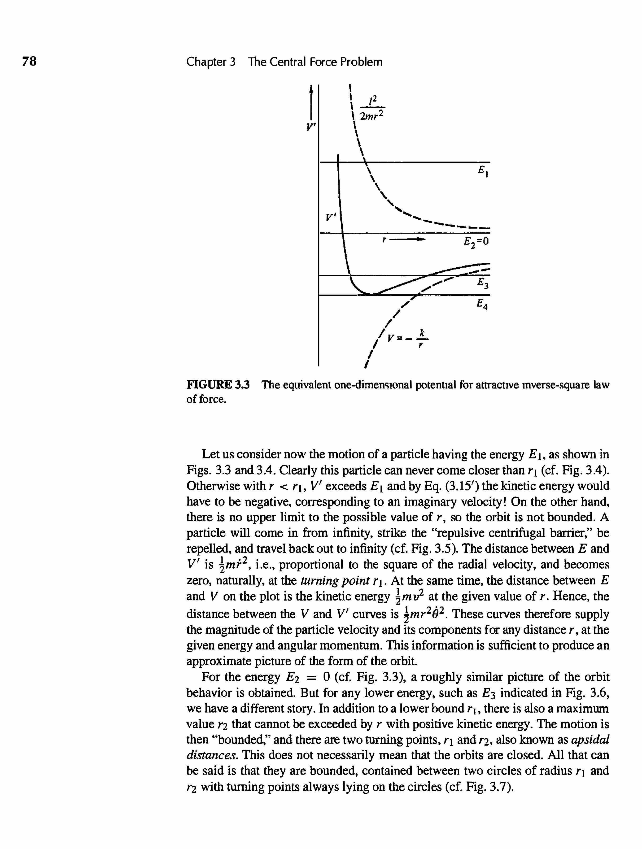
FIGURE 3.3 The equivalent one-dimen�1onal potential for attractive inverse-square law of force.

Let us consider now the motion of a particle having the energy E 1. as shown in Figs. 3.3 and 3.4. Clearly this particle can never come closer than r1 (cf. Fig. 3.4). Otherwise with r < r1, V' exceeds E 1 and by Eq. (3.15') the kinetic energy would have to be negative, corresponding to an imaginary velocity! On the other hand, there is no upper limit to the possible value of r, so the orbit is not bounded. A particle will come in from infinity, strike the ''repulsive centrifugal barrier," be repelled, and travel back out to infinity (cf. Fig. 3.5). The distance between E and V' is �mr2, i.e., proportional to the square of the radial velocity, and becomes zero, naturally, at the turning point r1• At the same time, the distance between E and V on the plot is the kinetic energy �mv2 at the given value of r. Hence, the

distance between the V and V' curves is �mr2ti2. These curves therefore supply � the magnitude of the particle velocity and its components for any distance r, at the given energy and angular momentum. This information is sufficient to produce an approxin1ate picture of the for111 of the orbit.

For the energy E2 = 0 (cf. Fig. 3.3), a roughly similar picture of the orbit behavior is obtained. But for any lower energy, such as £3 indicated in Fig. 3.6, we have a different story. In addition to a lower bound r1, there is also a maximum value r2 that cannot be exceeded by r with positive kinetic energy. The motion is then ''bounded," and there are two turning points, r1 and rz, also known as apsidal di.�tance.�. This does not necessarily mean that the orbits are closed. All that can be said is that they are bounded, contained between two circles of radius r1 and r2 with turning points always lying on the circles (cf. Fig. 3.7).

3.3 The Equivalent One-Dimensional Problem

V'

I I I I I I I

, ,

V'

79

1:.· I

1 mr2 2

r

FIGURE 3.4 Unbounded motion at positive energie� for inverse-square law of fo1ce.

FIGURE 3.5 The orbit for E 1 correspo11d1ng to unbounded motion.

80 Chapter 3 The Central Force Prob lem

V'

I I I I I I

'2 ----

1 , __ I I I I I

FIGURE 3.6 The equivalent one-dimensional potential for inver�e-�quare law of torce, 1llu�tratJ.ng bounded 1notion at negative energies.

If the energy is £4 at the minimum of the fictitious potential as shown in Fig. 3.8, then the two bounds coincide. In such case, motion is possible at only one radius; r = 0, and the orbit is a circle. Remembering that the effective ''force'' is the negative of the slope of the V' curve, the requirement for circular orbits is simply that f' be zero, or

z2 ·2 f (r) = - 3 = -mre . mr·

We have here the familiar elementary condition for a circular orbit, that the applied force be equal and opposite to the ''reversed effective force'' of centripetal

I I

-- --

- -

FIGURE 3.7 The nature of the orbits for bounded motion.

3.3 The Equivalent One-D1mens1onal Problem

V' '•

I I I I I I I I I I I

��

81

r

E4

FIGURE 3.8 The equivalent one-dimensio11al potential of 1nver&e-squai-e law of force, illustrat1ng the condition t"or circular orbit�.

acceleration.* The properties ot· circular orbits and the conditions for them will be studied in greater detail in Section 3.6.

Note that all of thil> discussion ot· the orbits for various energies has been at one value of the angular momentum. Changing l changes the quantitative details of the V' curve, but it does not affect the general classification of the types of orbits.

For the attractive inver!.e-square law of force discussed above, we shall see that the orbit for E1 is a hyperbola, for E2 a parabola, and for E3 an ellipse. With other forces the orbits may not have such simple forms. However, the same general qualitative division into open, bounded, and circular orbits will be true for any attractive potential that (1) falls off slower than 1/r2 as r ) oo, and ( 2) becomes infinite slower than 1/1·2 as r ) 0. The first condition en!>ures that the potential predominates over the centrifugal tem1 for large r, while the second condition is such that for small r it is the centrifugal tenn that is important.

The qualitative nature of the 1notion will be altered if the potential does not satisfy these requirements, but we may still use the method of the equivalent potential to examine features of the orbits. As an example, let us consider the attractive potential

a V(r) = - 3,

r

3a with f = - 4.

r

The energy diagram is then as shown in Fig. 3.9. For an energy E, the1·e are two possible types of motion, depending upon the initial value of r. If ro is less than

r1 the motion will be bounded, r will always remain less than r1, and the particle will pass through the center of force. It" r is initially greater than r2 , then it will

*The case E < £4 doe& nol correspond to physically possible mot1on, for then i·2 would have to be • • • • negative, or r 1mag1nary.


v \

12

I I I

\ 2rnr2 \ \ \ \ \ \

'1

" ' I I I

'2 -7"' / I

I V' /v

I

E

r

FIGURE 3.9 The eq111valent one-dimen�tonal potential t"or an attractive inver�e-fourth law of t"orce

always remain so; the mc>tion 1s unbounded, and the particle can never get inside the ''potential'' hole. The initial condition r1 < ro < rz is again not physically possible.

Another interesting example of the method occur& for a linear restoring force (isotropic harmonic oscillator):

f = -kr,

For zero angular momentum, cc>11esponding to motion along a straight line, V' = V and the situation is as shown in Fig. 3.10. For any positive energy the motion is bounded and, as we know. simple harmonic. If I =!= 0, we have the state of affairs shown in Fig. 3.1 1 . The motion then is always bounded for all physically possible

V'

V' = V=

I= 0

I kr2 2

E

r -

FIGURE 3.10 Eftecl1,1e potenllal for zero angular momentum.

3 .4 The Vir1al Theorem

l � 0

V' t \ \ v• \

:.;' E I / I I\ / I I // I I ' / I

I I ' / I z2 V- k 2 I ,><.;;. I -'--- r 1 / " I 2 2 ;...,,,. "· ·- I 2mr

- -- -

r --

83

FIGURE 3.11 The equivalent one-dimensional potential for a linear restonng force.

energies and does not pass through the center of force. In this particular case, it is easily seen that the orbit is elliptic, for if f = -kr, the x· and y-components of the force are

fx = -kx, f}' = -ky.

The total motion 1s thus the re5ultant of two simple hannonic oscillations at right angles, and of the same frequency, which in general leads to an elliptic orbit.

A well-known example is the spherical pendulum for small amplitudes. The familiar Lissajous figures are obtained as the composition of two sinusoidal oscillations at right angles where the ratio of the frequencies is a rational number. For two oscillations at the same frequency, the figure is a straight line when the oscillations are in phase, a circle when they are 90° out of phase, and an elliptic i:.hape otherwise. Thus, central force motion under a linear restoring force therefore provides the simplest of the Lissajous fig11res.

3.4 • THE VIRIAL THEOREM

Another property of central force motion can be derived as a special case of a general theorem valid for a large variety of systems the virial theorem. It differs in character from the theorems previously discussed in being statistical in nature; i.e., it i� concerned with the time averages of various mechanical quantities.

Consider a general system of mass points with position vectors r, and applied forces F, (including any t'orces of constraint). The fundamental equations of motion are then

p; = F,. (1.3)

We are interested in the quantity


G = LP1. r, . • I

where the summation is over all particles in the system. The total time derivative of this quantity is

dG '"°'. '"°'. dt

= L.., r, . p, + L.., p, • r,. I I

The first term can be transfo1·1r1ed to

I I I

while the second te11n by (l.3) is

L Pi • r, = L F1 • r,. I I

Equation (3.23) tl1erefore reduces to

d

dt L p, · r1 = 2T + L F, · r,. I I

(3.23)

(3.24)

The time average of Eq. (3. 24) over a time interval -r is obtained by integrating both sidei:. with respect to t from 0 to -r, and dividing by -r:

or

1 'dG dG -

d dt =

d = 2T + L F, • r, 1: 0 t t

l

1 2T + LF, · r; = - fG(-r) - G(O)J.

• I

(3.25)

If the motion is periodic, i.e., all coordinates repeat after a certain time, and it' -r is chosen to be the period, then the right-hand side of (3.25) vanishes. A similar conclusion can be reached even if the motion is not periodic, provided that the coordinates and velocities for all particles remain finite so that there is an upper bound to G. By choosing -r sufficiently long, the 1ight-hand side ofEq. (3.25) can be made as small as desired. In both cases, it then follows that

(3.26)

Equation (3.26) is known as the virial theorem, and the right-hand side is called the virial cif Clausius. In this fo1·1r1 the theorem is imporant in the kinetic theory

1.4 The V1rial Theorem 85

of gases 1.ince it can be used U) derive ideal gas law for perfect gases by means of

the following brief argument. We consider a gas consisting of N atoms confined within a container of vol

ume V. The gas is further assumed to be at a Kelvin temperature T (not to be confused with the symbol for kinetic energy). Then by the equipartition theorem ot· kinetic theory, the average kinetic energy ot· each atom is given by �kBT, kB

being the Boltzmann constant, a relation that in effect is the definition of temperature. Tue left-hand side ()f Eq. (3.26) is therefore

�NkBT.

On the right-hand side of Eq. (3.26), the forces Fi include both the forces of interaction between atoms and the torces of constraint on the sy stem. A perfect gas is defined as one for which the torces of interactic'n contribute negligibly to

the virial. This occurs, e.g., if the gas is so tenuous that collisions between atoms occur rarely, compared to collisions with the walls of the container. It is these walls that constitute the constraint on the system, and the forces of constraint, F c.

are localized at the wall and come into existence whenever a gas atom collides with the wall. The sutn on the right-hand side of Eq. (3.26) can therefore be replaced in the average by an integral over rhe surface ot· the container. The force of constraint represents the reaction of the wall to the collision forces exerted by the atoms on the wall, i.e., to the pressure P. With the usual outward convention for the unit vector n in the direction of the nor111al to the surface, we can therefore write

or

dF, = -PndA,

1 p 2LF,·ri=- 2 n·rdA. l

But, by Gauss's theorem,

n·rdA= V·rdV=3V.

The virial theorem, Eq. (3.26), for the system representing a perfect gas can therefore be written

which, cancelling the common factor of � on both sides. is the familiar ideal gas law. Where the interparticle forces contribute to the virial, the perfect gas law of course no longer holds. The virial theorem is then the principal tool, in classical kinetic theory, fc>r calculating the equation of state corresponding to such imperfect gases.


We can further show that if the force� F1 are the sum of nonfrictional forces F; and frictional forces f; proportional to the velocity, then the virial depends only on the F;; there is no contribution from the f,. Of course, the motion of the system must not be allowed to die down as a result of the frictional forces. Energy must constantly be pumped into the system to maintain the motion; otherwise all time averages would vanish as r increases indefinitely (cf. Derivation 1.)

If the forces are derivable from a potential, then the theorem becomes

- l " T = l .L.,, 'VV • r1, I

and for a single particle moving under a central force it reduces to

_ I av T = - r.

2 or

It" l-' is a power-law function of r,

V = arn+l,

where the exponent is chosen so that the force law goes as rn, then

and Eq. (3.28) becomes

av -r = (n + l)V, or

T=n+lv. 2

(3.27)

(3.28)

(3.29)

By an application of Euler's theorem for homogeneous functions (cf. p. 62), it is clear that Eq. (3.29) also holds whenever V is a homogeneous function in r of degree n + I . For the further special case of inverse-square law forces, n is - 2, and the virial theorem takes on a well-known fo11n:

3.5 • THE DIFFERENTIAL EQUATION FOR THE ORBIT,

AND INTEGRABLE POWER-LAW POTENTIALS

(3.30)

In treating specific details of actual central force problems, a change in the orientation of our discussion is desirable. Hitherto solving a problem has meant finding r and() as functions of time with E, l, etc., as constants of integration. But most ot"ten what we really seek is the equation of the orbit, i.e., the dependence of r upon (), eliminating the parameter t. For central force problems, the elimination is particularly simple, since t occurs in the equations of motion only as a variable of differentiation. Indeed, one equation of motion, (3.8), simply provides a definite

3 .5 The Differential Equation for the Orbit 87

relation between a differential change dt and the corresponding change de:

I dt = mr2 de. (3.31)

The co1·1esponding relation between derivatives with respect to t and e is

d l d (3.32) - - -..,- --

dt - m1·2 de·

These relations may be used to convert the equation of motion (3.12) or (3.16) to a differential equation for the orbit. A substitution into Eq. (3.12) gives a secondorder differential equation, while a substitution into Eq. (3.17) gives a simpler first-order differential equation.

The substitution into Eq. (3.12) yields

l d 1 dr r2 de mr2 de

12 - 3 = f (r), mr· (3.33)

which upon substituting u = 1/r and expressing the results in terrns of the potential gives

d2u m d 1

de2 + u = - z2 du v � .

(3.34)

The preceding equation is such that the resulting orbit is symmetric about two adjacent turning points. To prove this statement, note that if the orbit is symmetrical it should be possible to reflect it about the direction of the turning angle without producing any change. If the coordinates are chosen so that the turning point occurs for e = 0, then the reflection can be effected mathematically by substituting -e fore. The differential equation for the orbit, (3.34), is obviously invariant under such a substitution. Further the initial conditions, here

u = u(O), du

= 0, de 0

fore = 0,

will likewise be unaffected. Hence, the orbit equation must be the same whether expressed in te11ns of e or -e, which is the desired conclusion. The orbit i.f therefore invariant under reflection about the apsidal vector.f . In effect, this means that the complete orbit can be traced if the portion of the orbit between any two turning points is known. Reflection of the given portion about one of the apsidal vectors produces a neighboring stretch of the orbit, and this process can be repeated indefinitely until the rest of the orbit is completed, as illustrated in Fig. 3.12.

For any particular t'orce law, the actual equation of the orbit can be obtained by eliminating t trom the solution (3.17) by means of (3.31 ), resulting in

l dr de = ---;::.====== ·

mr2 l. E - V (1·) - 12 m 2mr2

(3.35)


-I �, I I \ \ \ \ \

FIGURE 3.12 Extension of the orbit by reflection of a portion about the aps1dal vector&.

With slight rearrangements, the integral of (3.35) is

r () = == + eo, 2mE 2mV I

,2 - /2 - 'i'2

d1· (3.36) ro r2

or, if the variable of integration is changed to u = 1 / r, u du • (3.37)

uo 21nE _ 2mV _ u2 /2 /2

As in the case of the equation of motion, Eq. (3.37), while solving the problem fo1mally, is not always a practicable solution, because the integral often cannot be expressed in terrns ot' well-known functions. In fact, only certain types of force laws have been investigated. The rnost important rue the po\ver-law functions of r,

V = ar11+1 (3.38) so that the force varies at the nth power of r. * With this potential, (3.37) becomes

,, du (3.39) --;:================ · II() 2111£ - 21n.a u-11-l - u2 /2 /2

This again is integrable in ter1ns of simple functions only in certain cases. The particular power-law exponents for v.1hich the results can be expressed in ter1ns of trigonometric function� are

n = 1, - 2, -3 .

._The case n = -1 1s to be excluded from the discussion. In the potential (3.38), It corresponds to a con�tant polenti.il, 1.e , no force at all It 1s an equally anomalou� c�e if the exponent is Ubed in the force law directly, �1nce a force varying as r-1 corresponds to a loganthm1c potential, which is not a power law at all. A loganthrruc potential is unusual for motion about a point, it is more characteristic

of a line source. Further detail� of the�e ca.�cs are given 1n the second edition of this text.

3.6 Conditions for Closed Orbits (Bertrand's Theorem)

The results of the integral for

n = 5, 3, 0, -4, -5, -7

89

can be expressed in terms of elliptic functions. These are all the possibilities for an integer exponent where the form.al integrations are expressed in te1·111s of simple well-known functions. Some fractional exponents can be '>hown to lead to elliptic functions, and many other exponents can be expressed in tenns of the hypergeometric function. The trigonometnc and elliptical functions are special cases of generalized hypergeometric function integrals. Equation (3.39) can of course be numerically integrated for a11y nonpathological potential, but thii> is beyond the scope of the text.

3.6 • CONDITIONS FOR CLOSED ORBITS (BERTRAND'S THEOREM)

We have not yet extracted all the information that can be obtained from the equivalent one-dimen<;ional problem or from the orbit equation without explicitly solving for the motion. In particular, it is possible to derive a powerful and thoughtprovoking theorem on the types of attractive central forces that lead to closed orbits, i.e., orbits in which the particle eventually retraces it<; own tootsteps.

Conditions have already been described for one kind of closed orbit, namely a circle about the center of force. For any given l, this will occur it· the equivalent potential V'(r) has a minimum or maximum at some distance r0 and if the energy Eis just equal to V1(ro). The requirement that V' have an extremum is equivalent to the varushing of /1 at ro, leading tt) the condition derived previously (cf. Section 3.3).

[2 f(ro) = - 3•

mr0 (3.40)

which says the force must be attractive for circular orbits to be possible. In addition, the energy of the particle must be given by

z2 E = V(ro) + 2• 2mr0

(3.41)

which, by Eq. (3. 15), co1·1e;;ponds to the requirement that for a circular orbit r is zero. Equations (3.40) and (3.41) are both elementary and familiar. Between them they imply that for any attractive central force it is possible to have a circular orbit at some arbitrary radius ro, provided the angular momentum l is given by Eq. (3.40) and the particle energy by Eq. (3.41).

The character of the circular orbit depends on whether the extremum of V' is a minimum, as in Fig. 3.8, or a maximum, as if Fig. 3.9. If the energy is slightly above that required for a circular orbit at the given value of l , then for a minimum in V' the motion, though no longer circular, will still be bounded. However, if


V' exhibit� a maximum, then the slightest raising of E above the circular value, Eq. (3.34), results in motion that is unbounded, with the particle moving both through the center of force and out to infinity for the potential shown in Fig. 3.9. Borrowing the terminology t'rom the case of static equilibriurn, the circular orbit arising in Fig. 3.8 is said to be .�table; that in Fig. 3.9 is unstable. The stability of the circular orbit is thus dete11nined by the sign of the second derivative of V' at the radius of the circle, bemg stable for positive second derivative (V' concave up) and unstable for V' concave down. A stable orbit therefore occurs if

o2v' af 312 2 = - "' + 4 > 0.

or r=ro u1· r=ro mro

Using Eq. (3.40), this condition can be written

or

of 01· r=1·0

3 f (1·0) < - --- ,

dlnf > -3 dlnr r=ro

(3.42)

(3.43)

(3.43')

where f(ro)/ ro is assumed to be negative and given by dividing Eq. (3.40) by ro. If the force behaves like a power law of 1· in the vicinity of' the circular radius r0,

f = -krn,

then the stability condition, Eq. (3.43), becomes

-knrn-l < 3krn-l

or

n > -3, (3.44)

where k is assumed to be po�itive. A power-law attractive potential varying more slowly than l/ r2 is thus capable of stable circular orbits for all values of ro.

If the circular orbit is stable, then a small increase in the particle energy above the value for a circular orbit results in only a slight variation of r about ro. It can be easily shown that for such small deviations t'rom the circularity conditions, the particle executes a o;;imple hannomc motion mu(= l/r) about uo:

U = Uo + a COS fje. (3.45)

Her·e a is an amplitude that depends upon the deviation of the energy fro1n the value for circular orbits, and f3 is a quantity arising from a Taylor series expansion

3.6 Cond1t1ons for Closed Orbits (Bertrand's Theorem) 91

of the t"orce law f (r) about the circular orbit radius ro. Dire"1: substitution into the force law gives

• (3.46)

As the radius vector of the particle sweeps completely around the plane, u gc>es through f3 cycles of its oscillation (cf. Fig. 3.13). If f3 is a rational number, the ratio of two integers, p / q, then after q revolutions of the radius vector the orbit would begin to retrace itself c;o that the orbit is closed.

At each ro such that the inequality in Eq. (3.43) is satisfied, it is possible to establish a <stable circular orbit by giving the particle an initial energy and angular momentum prescribed by Eqs. (3.40) and (3 .41). The question naturally a1ises as to what fo1·111 the force law must take in order that the slightly perturbed orbit about any of these circular orbits c;hould be closed. It is clear that under the�e conditions f3 must not only be a rational number, it must also be the .�ame rational number at all distances that a circular orbit is possible. Otherwise, since f3 can take on only di�crete values, the number of oscillatory periods would change discontinuously with 1·0, and indeed the orbits could not be closed at the discontinuity. With {32 everywhere ct>nstant, the defining equation t"or {:J2, Eq. (3.46), becomes in effect a differential equation for the force la\V j in terms of the independent van able ro.

We can indeed con�ider Eq. (3.46) to be written in terrns of r if we keep in mind that the equation is valid only over the ranges in r for which stable circular orbits are possible. A slight rearrangement of Eq. (3.46) leads to the equation

I

I I

I

dlnf =

{32 _ 3, dlnr

/' /

- . '

\ \

\ '

' �-..... /

I I

(3.47)

FIGURE 3.13 Orbit for motion in a central force deviating slightly from a circular orbit for f3 = 5.


which can be immediately integrated to give a force law:

k f (r) = - ,.3-p2. (3.48)

All torce laws of this fo1·111, with f3 a rational number, lead to closed stable orbits t'or initial conditions that differ only slightly from conditions defining a circular orbit. Included within the possibilities allowed by Eq. (3.48) are some familiar torces such as the inverse-square law (/3 = l ), but of course many other behaviors, such as f = -kr-219({3 = i), are also per1nitted.

Suppose the initial conditions deviate more than slightly from the requirementc;; t'or circular orbits; will these same force laws still give circular orbits? The question can be answered directly by keeping an additional te11n in the Taylor series expansion of the force Jaw and solving the resultant orbit equation.

J. Bertrand solved this problem in 1873 and found that for mc>re than first-order deviations from circularity, the orbits are closed only for {32 = 1 and {32 = 4. The first of these values ot' {32, by Eq. (3.48), leads to the familiar attractive inversesquare law; the second is an attractive force proportional to the radial distance� Hooke's law! These force laws, and only these, could possibly produce closed orbits for any arbitrary combination of l and E(E < 0), and in fact we know fron1 direct !-.olution of the orbit equation that they do. Hence, we have Bertrand's theorem: The only central forces that result tn closed orbit.1',f<Jr all b<Jund particles are the inverse-square law and Hooke's la�v.

This is a remarkable result, well worth the tedious algebra required. It is a commonplace astronomical observation that bound celestial objects move in orbitc; that are in first approximation closed. For the most part, the small deviations from a closed orbit are traceable tt> perturbations such as the presence of other bodies. The prevalence ot· closed orbits holds true whether we consider only the solar system, t)r look to the many examples of true binary stars that have been observed. Now, Hooke's law is a most unrealistic force law to hold at all distances, for it implies a force increasing indefinitely to infinity. Thus, the existence of closed orbits t'or a wide range of initial conditions by itself leads to the conclusion that the gravitational force varies as the inverse-square of the distance.

We can phrase this conclusion in a slightly dift'erent manner, one that is of somewhat more significance in modem physics. The orbital motion in a plane can be looked on as compounded of two oscillatory motions, one in r and one in () with the same period. The cha1·acter <Jf <Jrbit.� in a gravitational field fixes the form of the force law. Later on we shall encounter other fo1111ulations of the relation bet\veen degeneracy and the nature of the potential.

3.7 • THE KEPLER PROBLEM: INVERSE-SQUARE LAW OF FORCE

The inverse-square law is the most important of all the central force laws, and it deserves detailed treatment. For this case, the force and potential can be written

3.7 The Kepler Problem: Inverse-Square Law of Force

as

k /=-2 r

k V - --- . r

93

(3.49)

There are several ways to integrate the equation for the orbit, the simplest being to substitute (3.49) in the differential equation for the orbit (3.33). Another approach is to start with Eq. (3.39) with n set equal to -2 t"or the gravitational force

e =e' - du -;:.======· 2mE + 2mku _ u2 /2 /2

(3.50)

where the integral is now taken as indefinite. The quantity ()' appearing in (3.50) is a constant of integration deter111ined by the initial conditions and will not necessarily be the same as the initial angle 80 at time t = 0. The indefinite integral is ot· the standard fo11n,

where

dx 1 f3 +2yx ---;:::===== = ---r= arc cos- --- , Ja +.Bx+ yx2 -y y'q

q = {32 - 4ay.

To apply this to (3.50), we must set

2mE 2mk .B = [2 a= [2 , y = -1,

and the discrinrinant q 1s therefore

q = 2mk 2 [2

'

2El2 I+ -

mk2 •

With these sub<;titutef., Eq. (3.50) becomes

12,, - 1 () = ()' - arc co<, -rm=k===;=·

1 + 2E/2 mk2

Finally, by solving fo1 u, = 1/ r, the equation of the orbit is found to be

1 -- -r

mk [2 1+

2£/2 1 + mk2 cos(e - e') .

(3.51)

(3.52)

(3.53)

(3.54)

(3.55)

The constant of integration()' can now be identified from Eq. (3.55) as one of the turning angles of the orbit. Note that only three of the four constants of integration appear in the orbit equation; this is always a characteristic property of the orbit. In


effect, the fourth constant locates the initial position of the particle on the orbit. If we are interested solely in the orbit equation, this info1111ation is clearly irrelevant and hence does not appear in the answer. Of course, the missing e<>nstant has to be supplied if we wish to complete the solution by finding r and () as functions of time. Thus, if we choose to integrate the conservation theorem for angular rnomentum,

mr2 d() = l dt,

by means of (3.55), we must additionally specit·y the initial angle eo. Now, the general equation of a conic with one focus at the origin is

l - = C[l + e cos(() - ()')] , r

(3.56)

where e is the eccentricity of the conic section. By comparison with Eq. (3.55), it follows that the orbit is always a conic section, with the eccentricity

e = 2£[2

I + mk2 . (3.57)

The nature of the orbit depends upon the magnitude of e according to the following scheme:

e > 1 . e = l , e < 1,

e = 0,

E > 0: E = 0: E < 0:

mk2 E - .

- - 2/2 •

hyperbola, parabola, ellipse,

circle.

This classification agrees with the qualitative discussion of the orbits on the energy diagram of the equivalent one-dimensional potential V'. The condition for circular motion appears here in a somewhat different form, but it can easily be derived as a consequence of the previous conditions for circularity. For a circular orbit, T and V are constant in time, and from the virial theorem

Hence

k E - -

- 2ro · (3.58)

But from Eq. (3.41), the statement of equilibrium between the central force and the ''eft"ective force," we can write

k 12 � = _...,. r2 mr3 ' 0 0


or

!2 ro = .

mk

With this for11·1ula for the orbital radius, Eq. (3.58) becomes

mk2 E = - 212 '

the above condition for circular motion.

95

(3.59)

In the case of elliptic orbits, it can be shown the major axi� depends solely upon the energy, a theorem of considerable importance in the Bohr theory of the atom. The semimajor axis is one-half the sum of the two apsidal distances r1 and r2 (cf. Fig. 3.6). By definition, the radial velocity is zero at these points, and the conservation of energy implies that the apsidal distances are therefore the root<; of the equation (cf. Eq. (3. 15) )

or

12 k E - + - = 0, 2mr2 ,.

k [2 r2 + r - = 0.

E 2m E (3.60)

Now, the coefficient of the linear term in a quadratic equation is the negative of the �um of the roots. Hence, the sernimajor axis is given by

r1 + r2 k a = = - -

2 2E ' (3.61)

Note that in the circular limit, Eq. (3.61 ) agrees with Eq. (3.58). In ter111s of the semimajor axis, the eccentricity of the ellipse can be written

e = z2 I - '

mka (3.62)

(a relation we will have use for in a later chapter). Further, from Eq. (3.62) we have the expression

[2 - = a(l - e2) , mk

in te1111s of which the elliptical orbit equation (3.55) can be written

a(l - e2) r = .

l + e cos(e - e')

(3.63)

(3.64)


t; = 0 E = 0.5

I!. = 0 75

E = 0.9

FIGURE 3.14 Ellipses with the same major axes and eccentncities from 0.0 to 0.9.

From Eq. (3.64), 1t follows that the two apsidal distances (which occur when e - e' is 0 and n, respectively) are equal to a(l - e) and a( l + e), a� is to be expected from the properties of an ellipse.

Figure 3. 14 shows sketches of four elliptical orbits with the same major axis a, and hence the same energy, but with eccentricities s = 0.0, 0.5, 0.75, and 0.9. Figure 3. 15 shows how r1 and r2 depend on the eccentricity e.

The velocity vector v11 of the particle along the elliptical path can be resolved • into a radial component Vr = r = Pr Im plu!> an angular CC>mponent v9 = re = l /mr

� VII = Vrf + V9 6.

The radial component with the magnitude vr = svo sin e /(1 - e2) vanishes at the two apsidal distances, while v9 attains its maximum value at perihelion and its minimum at aphelion. Table 3. 1 lists angular velocity values at the apsidal distances t"or several eccentricities. Figure 3. 1 6 presents plots of the radial velocity component Vr versu<; the radius vector r for the half cycle when Vr points outward, i.e., it is positive. During the remaining half cycle Vr is nega-

2

aphelion distance

J{' I perihelion d1�tance

0 0 c I

FIGURE 3.15 Dependence ot' no11r1alized ap�1dal di�tances r1 (lower line) and rz (upper line) on the eccentricity s .


• •

97

TABLE 3.1 No11·11alit:ed angular speeds () and v9 = r() at perihelion (r1) and aphelion (r2), re�pect1vely, rn Keplerian orbits ot' vanou:. eccentr1cittes (F.). The no1111alized radial distances at perihelion and aphelion are listed in columns 2 and 3, re:.pectJvely. The nonnalization ts with respect to motion in a circle with the radius a and the angular n1011ientun1 l = mavo = ma29o.

Eccentricity Penhel1on Aphelion Angular :.peed Linear angular speed • • • •

r1 /a r2/a 81 /fJo fJz/fJo v91 /vo v92/vo

I - I" 1 l l 1

s l + e ( 1 - e)2 (1 + e)2 1 - e l + s

0 1 I 1 1 l 1

0. 1 0.9 I . I 1.234 0.826 l . l I l 0.909 0.3 0.7 1 .3 2 041 0.592 1 .429 0.769 0.5 0.5 1.5 4 000 0.444 2.000 0.667 0 7 0.3 1 .7 l l . 1 1 1 0.346 3.333 0.588

0.9 0. 1 1 .9 100.000 0.277 10.000 0.526

tive, and the plot of Fig. 3.1 6 repeats itself for the negative range below t'r = 0 (not shown). Figure 3. 1 7 shows analogous plots of the angular velocity component ve versus the angle e. In these plots and 1n the table the velociues are

• normalized relative to the quantities vo and Bo obtained from the expressions l = mr20 = mrv9 = ma20o = mavo f"or the conservation of angular momentum in the elliptic orbits of semimajor axis a, and in the circle of radius a.

0.6 -

0.4

0 2 -

o --

().5

c = 0 5

/,,-.....s = O 3

,g = 0 l / ' \

I ,. ;;;

I 5

FIGURE 3.16 No1111alized radial velocity, vr. versus r for three valuei:. of the eccentricity e.


2

S = 0 5

--- s = 0.3 1-

l' = 0 1

0 J OO 300

FIGURE 3.17 No1111al1zed orbital velocity, ve, versus e tor three values of the eccentricity e.

3.8 • THE MOTION IN TIME IN THE KEPLER PROBLEM

The orbital equation for motion in a central inverse-square force law can thus be solved in a fairly straightforward manner with results that can be stated in simple closed expressions. Describing the motion of the particle in time a-; it traverses the orbit is however a much more involved matter. In principle, the relation between the radial distance of the particle r and the time (relative to some f..tarting point) is given by Eq. (3 . 1 8), which here takes on the form

m r dr (3.65) t =

2 ro --;:::======== · k /2

r - 2mr2 + E Similarly, the polar angle () and the time are connected through the conserva

tion of angular momentum,

mr2 dt = l d(),

which combined with the orbit equation (3.5 1 ) leads to

t3 e d() t = --

mk2 Bo [ 1 + e cos(() - ()')]2 · (3.66)

Either of these integrals can be carried out in te1111s of elementary functions. However, the relations are very complex, and their inversions to give r or () as functions of t pose for11ridable problems, especially when one wants the high precision needed for astronomical observations.

To illustrate some of these involvements, let us consider the situation for parabolic motion (e = 1 ), where the integrations can be most simply carried out. It is customary to measure the plane polar angle from the radius vector at

3.8 The Motion in Time i n the Kepler Prob lem 99

the point of closest approach a point most usually designated as the perihelion.* This convention corresponds to setting e' in the orbit equation (3.5 1 ) equal to zero. Correspondingly, time is measured from the moment, T , of perihelion passage. Using the trigonometric identity

() 1 + cos e = 2 cos2 - ,

2

Eq. (3.66) then reduces for parabolic motion to the fo1111

z3 e e t =

2 sec4 - de.

4mk o 2

The integration is easily perfo1·111ed by a change of variable to x = tan(() /2), leading to the integral

t3 t = ---=-2mk2 o

tan(B/2)

(1 + x2) dx,

or

z3 t

= 2mk2

(3.67)

In this equation, -TC < e < TC , where for t > -oo the particle starts approaching from infinitely far away located at e = -TC . The time t = 0 corresponds to () = 0, where the particle is at perihelion. Finally t --* +oo corresponds to e ) TC as the particle moves infinitely far away. This is a straightforward relation t'or t as a function of e ; inversion to obtain () at a given time requires solving a cubic equation for tan(61 /2), then finding the corresponding arctan. The radial distance at a gi,1en ti1ne is given through the orbital equation.

For elliptical motion, Eq. (3.65) is most conveniently integrated through an auxiliary variable i/f, denoted as the eccentric anomaly,* and defined by the relation

r = a( l - e cos i/f ) . (3.68)

By comparison with the orbit equation, (3.64), it is clear that i/f also covers the interval 0 to 2n as () goes through a complete revolution, and that the perihelion occurs at i/f = 0 (where e = 0 by convention) and the aphelion at i/f = TC = e.

'l<L1terally, the tel'tr1 �hould be restnctcd to orbit� around the Sun, whtle the more gener.il te1111 �hould

be periap.\·i.•. However, 1t ha� become customary to use perJ.hellon no matter where the center of force

1s Eve11 for space craft orbiting the Moon, official descnptionb of the orb1t.tl parameter<; refer to

perihelion where pericynthion would be the pedantic te1111 *Medieval astronomers expected the angular motion to be constant. The angle calculated by mulnplying th.ts average angular velocity (2ir /period) by the time since the la�t perihelion pa�sage was called the meJn mom.ily From the me.in anomaly the eccentnc anomaly could be calculated and then used to calculate the true anomaly. The angle e 1� called the true anomaly JUSt as it was in medieval

astronomy.

1 00 Chapter 3 The Central Force Problem

Expressing E and e in terms of a, e, and k, Eq. (3.65) can be rewritten for elliptic motion as

m r r dr t = -

2k ro --;===r=2==a=(l=-=e2:==) ' r - za - 2

(3.69)

where, by the convention on the starting time, ro is the perihelion distance. Substitution of r in ter1ns of if! from Eq. (3.68) reduces this integral, after some algebra, to the simple fo1'lrt

I = ma3

k 0

1f; (1 - e cos if!) difr. (3 .70)

First, we may note that Eq. (3.70) provides an expression for the period, •, of elliptical motion, if the i11tegral is carried over the full range in if! of 2n:

'r - 2rra3/2 m -

k . (3. 71 )

This important result can also be obtained directly from the properties of an ell1pse. From the conse1vation of angular momentum, the areal velocity is constant and is given by

dA l 2 l dt = 2

r e = 2m . (3.72)

The area of the orbit, A, is to be found by integrating (3.72) over a complete period •:

Now, the area of an ellipse is

• dA l• - dt = A = . o dt 2m

A = nab,

where, by the definition of eccentr·icity, the semiminor axis b is related to a according to the fo11nula

b = a./I - e2 •

By (3.62), the semiminor axis can also be written as

b = al/2 z2 mk '

3.8 The Motion in Time in the Kepler Problem

and the period is therefore

• = 2m na3/2 I

[2 m - = 2na312 mk k '

1 01

as was found previously. Equation (3.71) states that, other things being equal, the square tlf the period is proportional to the cube of the major axis, and this conclusion is often referred to as the third of Kepler's laws.* Actually, Kepler was concerned with the specific problem of planetary motion in the gravitational field of the Sun. A more precise statement of this third law would therefore be: The square of the periods of the various planets are proporti(Jnal to the cube of thei1· major axes. In this fortn, the law is only approximately true. Recall that the motion of a planet about the Sun i� a two-body problem and m in (3.7 1) must be replaced by the reduced mass: (cf. Eq. (3.4))

where m1 may be taken as referring to the planet and m2 to the Sun. Further, the gravitational law of attraction is

so that the constant k is

(3.73)

Under these conditions, (3.7 1) becomes

2na312 (3.74) 0 = ,JG(m1 + m2) � -;::;G:::=m=2 '

if we neglect the m�s of the planet compared to the Sun. It is the approximate version of Eq. (3.74) that is Kepler's third law, for it states that • is proportional to a312, with the same constant of proportionality for all planets . However, the planetary mass m1 is not always completely negligible compared to the Sun's; for example, Jupiter has a mass of about O.lo/o of the mass of the Sun. On the other hand, Kepler's third law i� rigorously true for the electron orbits in the Bohr atom, since µ and k are then the same for all orbit� in a given atom.

To return to the general problem of the position in time t'or an elliptic orbit, we may rewrite Eq. (3.70) slightly by introducing the frequency of revolution w as

tKepler's three laws of planetary motion, publihhed around 1610, were the rehult of lus p1oneenng analysis of planetary ob�ervations and Ja1d the groundwork for Newton'� great advance.� The second law, the conservation ot are<1l velocity. 1� a general theorem for central force motion, a� h� been noted previously. However, the first that the planets move 1n ellipt1cal orbith about the Sun at one

focus and the third are restricted specifically to the inverse-�quare Jaw of force.


2.rr w = - = r

k ma3 • (3.75)

The integration in Eq. (3.70) is ot' course easily performed, resulting in the relation

wt = if! - e sin if!, (3.76)

known as Kepler's equation. The quantity wt goes through the range 0 to 2.rr , along with if! and e, in the course ot· a complete orbital revolution and is therefore also denoted as an anomaly, specifically the mean anomaly.

To find the position in orbit at a given time t, Kepler's equation, (3.76), would first be inverted to obtain the corresponding eccentric anomaly if!. Equation (3.68) then yields the radial distance, while the polar angle e can be expressed in ter1ns of if! by comparing the defining equation (3.68) with the orbit equation (3.64 ):

1 - e2 l + e cos e = .

I - e cos 1/1

With a little algebraic manipulation, this can be simplified, to

cos if! - e cos e = .

1 - e cos if! (3.77)

By successively adding and subtracting both sides of Eq. (3.77) from unity and taking the ratio of the resulting two equations, \Ve are led to the alternative forn1

e tan - = 2

l + e if! tan 2 .

1 - e (3.78)

Either Eq. (3.77) or (3.78) thus provides e, once if! is known. The solution ot· the transcendental Kepler's equation (3.76) to give the value of if! corresponding to a given time is a problem that has attracted the attention of many famous mathematicians ever since Kepler posed the question early in the seventeenth century. Newton, for example, contributed what today would be called an analog solution. Indeed, it can be claimed that the practical need to solve Kepler's equation to accuracies of a second of arc over the whole range of eccentricity fathered many of the developments in numerical mathematics in the eighteenth and nineteenth centuries. A few of the more than 1 00 methods of solution developed in the precomputer era are considered in the exercises to this chapter.

3.9 • THE LAPLACE-RUNGE-LENZ VECTOR

The Kepler problem is also distinguished by the existence of an additional conserved vector besides the angular momentum. For a general central force, New-

3.9 The Laplace-Runge-Lenz Vector

ton's second law of mot:J.on can be written vectorially as

. f r p = (r) - . ,.

1 03

(3 .79)

The cross product of i> with the constant angular momentum vector L therefore can be expanded as

. L

mf (r) . p x = [r x (r x r)] r

m f (r ) . 2 · = r(r · r) - r r . r Equation (3.80) can be further simplified by noting that

. 1 d r . r = - (r . r) = r r

2 dt

(3. 80)

(or, in less for1nal ter1ns, the component of the velocity in the radial direction is f ). As L is constant, Eq. (3.80) can then be rewritten, after a little manipulation, as

or

d (p x IJ) = -m f (r)r2 ! -rr2• •

dt · r r

d (p x L) = -mf (r )r2 d .!: .

dt dt r (3 .81)

Without specifying the fo1·1n of f (r ), we can go no further. But Eq. (3.8 1 ) can be immediately integrated if f (r ) is inversely proportional to r2 the Kepler problem. Writing f (r) in the form prescribed by Eq. (3 .49), Eq. (3 .81) then becomes

d d dt

(p x L) = dt

mkr r '

which says that for the Kepler problem there exists a conserved vector A defined by

r A = p x L - mk - . r (3.82)

The relationships between the three vectors in Eq. (3.82) and the conservation of A are illustrated in Fig. 3. 1 8, which shows the three vectors at different positions in the orbit. In recent times, the vector A has become known amongst physicists as the Runge-Lenz vector, but priority belongs to Laplace.

From the definition of A, we can easily see that

A · L = 0, (3.83)

since L is perpendicular to p x L and r is perpendicular to L = r x p. It follows from this orthogonality of A to L that A must be some fixed vector in the plane of


A --

mk

p X L p

p X L 111k

A

P p X L A ---

FIGURE 3.18 The vectors p, L, and A at three positions 1n a Keplenan orbit. At penhelion (extreme let't) IP x LI = mk(l +e) and at aphelion (extreme right) Ip x LI = mk(l -e). The vector A always points tn the same direction with a magrutude mke.

the oro1t. lr & '1s used to denote the ang)e 'between r and the nxea Cl1rect1on or A., then the dot product of r and A is given by

A · r = At· cos e = r · (p x L) - mkr.

Now, by pe1·1nutation of the te1·1ns in the triple dot product, we have

r · (p x L) = L · (r x p) = /2 ,

so that Eq. (3.84) becomes

or

Ar Cose = l2 - mkr,

l mk - -..,..-

;: - z2 A ) + cos l1 . mk

(3.84)

The Laplace-Runge-Lenz vector thus provides still anl)ther way of deriving the orbit equation for the Kepler problem! Comparing Eq. (3.85) with the orbit equation in the fo1·1n of Eq. (3.55) shows that A is in the direction of the radius vector to the perihelion point on the orbit, and has a magnitude

A = mke. (3.86)

For the Kepler problem \Ve have thus identified two vector constants of the motion L and A, and a scalar E. Since a vector must have all three independent components, this corresponds to seven conserved quantities in all. Now, a system such as this with three degrees of freedom has six independent constants of the motion, corresponding, say to the three components of both the initial position

3 .9 The Laplace-Runge-Lenz Vector 1 05

and the initial velocity of the particle. Further, the constants of the motion we have found are all algebraic functions of r and p that describe the orbit as a whole (orientation in space, eccentricity, etc.); none of these seven con�erved quantities relate to where the particle is located in the orbit at the initial time. Since one constant of the motion must relate to this information, say in the form of T . the time of the perihelion passage, there can be only five independent constant� of the motion describing the size, shape, and 01·ientation of the orbit. We can therefore conclude that not all of the quantities making up L, A, and E can be independent; there must in fact be two relations connecting these quantities. One o;;uch relation has already been obtained as the orthogonality of A and L, Eq. (3.83). The other t"ollows from Eq. (3.86) when the eccentricity is expressed in ter1ns of E and l from Eq. (3.57), leading to

(3.87)

thus confi1·111ing that there are only five independent constants out of the seven. The angular momentum vector and the energy alone contain only four inde

pendent constants of the motion: The Laplace-Runge-Lenz vector thus adds one more. It is natural to ask why there should not exist for any general central force law some conserved quantity that together with L and E serves to define the orbit in a manner similar to the Laplace-Runge-Lenz vector for the special case of the Kepler problem. The answer seems to be that such conserved quantities can in t"act be constructed, but that they are in general rather peculiar functions of the motion. The constants of the motion relating to the orbit between them define the orbit, i.e., lead to the orbit equation giving r as a function of e. We have �een that in general orbits for central force motion are not closed; the arguments of Section 3.6 show that closed orbits imply rather stringent conditions on the form of the force law. It is a property of nonclosed orbits that the curve will eventually pass through any arbitrary (r, 6) point that lies between the bounds of the turning points of r. Intuitively this can be seen from the nonclosed nature of the orbit; as e goes around a full cycle, the particle must never 1·etrace its footsteps on any previous orbit. Thus, the orbit equation is such that r is a multivalued function of e (modulo 2n); in fact, it is an infinite-valued function of e. The corresponding conserved quantity additional to L and E defining the orbit must similarly involve an infinite-valued function of the particle motion. Suppose the r variable is periodic with angular frequency w, and the angular coordinate e is periodic with angular frequency WB . If these two frequencies have a ratio (wr/wB) that is an integer or integer fraction, periods are said to be commensurate. Commensurate orbits are closed with the orbiting n1ass continually retracing its path. When we > wr the orbit will spiral abc>ut the origin as the distance varies between the apsidal (maximum and minimum) values, closing c>nly if the frequencies are commensurate. If, as in the Kepler problem, wr = we, the periods are said to be degenerate. If the orbits are degenerate there exists an additional conserved quantity that is an algebraic function of r and p, such as the Runge-Lenz vector.

From these arguments we would expect a simple analog of such a vector to exist for the case of a Hooke's Jaw force, where, as we have seen. the orbits are


also degenerate. This is indeed the case, except that the natural way to fo1·111ulate the constant of the motion leads not to a vector but to a tensor of the second rank (cf. Section 7.5). Thus, the exi�tence of an additional constant or integral of the motion, be)1ond E and L, that is a simple algebraic function of the motion is sufficient to indicate that the motion is degenerate and the bounded orbits are closed

3.1 0 • SCATIERING IN A CENTRAL FORCE FIELD

Historically, the interest in central forces arose out of the astronomical proble:tns of planetary motion. There is no reason, however, why central force motion must be thclught of only in ter1ns of such problemr,; mention has already been made of the orbits in the Bohr atom. Another field that can be in\.estigated in terms of classical mechanics is the scattering of particles by central force fields. Of course, if the partJ.cles are on the atomic scale, it must be expected that the specific results of a classical treatment will often be incorrect physically, for quantum effects are usually large in such regions. Nevertheless, many classical predictions remain valid to a good approximation. More important, the procedures for describing scattering phenomena are the same whether the mechanics is classical or quantum; we can learn to speak the language equally as well on the basis of classical physics.

In its one-body for·1nulation, the scattering problem is concerned with the scattering of particles by a center <Jf f<J1r:e. We consider a uniform beam of particleswhether electrons, or a-particles. or planets is irrelevant all of the same mass and energy incident upon a center of force. It will be assumed that the t'orce falls off to zero t'or very large distances. The incident beam is characterized by specif yi11g ill) internity I (all)u call�tl flux d�nsity), which gives the number of particles crossing unit a1·ea normal to the beam in unit time. As a particle approaches the center of force, it will be either attracted or repelled, and its orbit will deviate from the incident straight-line trajectory. After passing the center of force, the force acting on the particle will eventually diminish so that the orbit once again approaches a straight line. In general, the final direction of motion is not the sa11e as the incident direction. and the particle is said to be scattered. The cro.�.� .�ect1on for scc.ttering in a gii·en direction, a(fi), is defined by

fl number of particles scattered into solid angle d Q per unit time a( ) dQ = . 'd . . ,

1nc1 ent 1ntens1ty (3.88)

whe1·e dn is a11 ele111e11t of solid ai1gle i11 tl1e ui1cctil111 a. Oft�11 a (fi) ii) dl:su dt:l)ignated as the differential scattering cross �·ection. With central forces there must be complete symmetry around the axis of the incident beam; hence the element of solid angle can be written

dr2 = 2rr sin e de , (3.89)

3.1 0 Scattering in a Central Force Field

s

ds

1 07

I I

FIGURE 3.19 Scatte1 i11g of an incident beam of particle.� by a center of force.

where e is tl1e ai.1gle belwee11 I.lie 1-caltered and incident directions, known as the scattering angle (cf. Fig. 3 . 19, where repulsive scattering is illustrated). Note that the name ''cross section'' is deserved in that <F (fi) has the dimensions of an area.

For any given particle the constants of the orbit, and hence the amount of scattering, are dete1·n1ined by its energy and angular momentum. It is convenient to express the angular momentum in te1·111s of the energy and a quantity known as the impact parameter, s, defined as the perpendicular distance between the center of force and the incident velocity. If vo is the incident speed of the particle, then

l = mvo.� = s.J2mE. (3.90)

Once E and .� are fixed, the angle of scattering E> is then determined uniquely. -t<

For the moment, it will be assumed that different values of s cannot lead to the same scattering angle. Therefore, the number of particles scattered into a solid angle dn lying betwee11 e and e + de must be equal to the number of the incident particles with impact parameter lying between the cor1esponding .1· and s + d.� :

2Jr /.� lds l = 2rra(B)I sin e I d81. (3.9 1 )

Absolute value signs are introduced in Eq. (3.9 1) because numbers of particles must of course always be positive, while s and e often vary in opposite directions. If s is considered as a function of the energy and the corresponding scattering angle,

.� = s(e, E), (3.92)

"It 1 � at th1. point m the fo1111ulc1.t1on that classical and quantum n1echanics part company. Indeed,

it is fundamentally characteristic of quantum mechan1cb that we cannot unequivocally predict the

trajectory of any particular par1i1..le. We can 011ly gJ\'e prcbabilities tor �cattering in variou� directions.


FIGURE 3.20 Relation of orbit parameter5 and scattering angle 111 a11 example of repul-• s1ve �cattermg.

then the dependence of the differential cross section on e is given by

s ds a (B) = . sin e dB

(3.93)

A fo1·1nal expression for the scattering angle E-) as a function of s can be directly obtained from the orbit equation, Eq. (3.36). Again, for simplicity, we will consider the case of purely repulsive scattering (cf. Fig. 3 20). As the orbit must be S)mmetric about the directi()n of the periapsis, the scattering angle is given by

8 = Jr - 2\11, (3.94)

where \II is the angle between the direction of the incoDl!ng asymptote and the periapsis (closest approach) directicln. In turn, \JI can be obtained from Eq. (3.36) by setting ro = 00 when e() = Jr (the incoming directionl, whence e = Jr - w wl1t:11 r = rm, tilt: ili1>l<lr1ct: uf clu1>t:1>L appruach. A Lrivial rt:arrangt:111t:nl ll1t:n lt:ad� t()

00 d1· (3.95) W =

r,,, r2 -r======= · 2ra E 2n1 V 1 /2 - /2 - ;-r

Expressing l in te1·1nr. 0f the impact parameter s (Eq. (3.90)). the resultant expression for 8(s) is

oc s dr 8 (.�) = Jr - 2 r,,, r ,2 ' - .r;; -

or, changing r tc> I ju

ll111 .� du e�s) = Jr - 2 ---;======= · 0

• (3.96)

(3.97)

3 . 1 0 Scattering 1n a Central Force Field 1 09

Equations (3. 96) and (3.97) are rarely used except for direct numerical computation of the scattering angle. However, when an analytic expression is available for the orbits, the relation between e and s can often be obtained almost by inspection. An historically important illustration of such a procedure is the repulsive scattering of charged particles by a Coulomb tield. The scattering force field is that produced by a fixed charge -Ze acting on the incident particles having a charge

-Z' e so that the force can be written as

ZZ'e2 f = -..,,-2- · r

i .e., a repulsive inverse-square law. The results of Section 3 .7 can be taken over here with no more change that writing the force constant as

k = -ZZ'e2. (3.98)

The energy E is greater tl1a11 zero, a11d tl1e 01·bit is a l1ype1bola witl1 tl1e ecce11tlicit)

given by"

E = 2£/2 1 + = m(ZZ1e2)2

l + 2Es ZZ'e

2

, (3.99)

where use has been made of Eq. (3.90). If (J' in Eq. (3.55) is chosen to be Jr . periapsis corresponds to e = 0 and the orbit equation becomes

1 mZZ'e -;: =

12 (E COS (J - 1). (3. 100)

Tlri� hyperbolic orbit equation ha." the same fo1111 as the elliptic orbit equation (3.56) except for a change in sign. The direction of the incoming asymptote. W , is then deter111ined by the condition r -+ oo:

or, by Eq. (3.94),

Hence,

and using Eq. (3 .99)

l cos W = -

E

• e I sin -

2 = ; ·

e cot2 = E2 - 1 , 2

*To avoid confu�ron \\'Ith the electron charge e, the eccentnc1ty w1ll temporanly be denoted by "·

1 1 0 Chapter 3 The Central Force Problem

e 2Es cot 2 = ZZ'e ·

The desired functional relationship between the impact parameter and the scatteri11g a11gle is tl1e1efo1e

ZZ'e2 8 s = 2E cot 2 , (3 . 10 1 )

so that on carrying through the manipulation required by Eq. (3.93), we find that o- (8) is given by

I a (8) = -

4

ZZ'e2 2E

2 4 8

csc 2 . (3. 102)

Equation (3.102) gives the famous Rutherford scattering cross section, originally denved by Rutherford for the scattering of a particles by atomic nuclei. Quantum mechanics in the nonrelativistic limit yields a cross section identical with this classical result.

as In atomic physics, the concept of a total .�cattering cr<Jss sel·tion O"T , defined

a·1· = a (fi) dQ. = 2n. 4n 0

Jr

a (8) sin (") de.

is of considerable importance. However, if we attempt to calculate the total cross section for Coulomb scattering by substituting Eq. (3. l 02) in this definition, we obtain an infinite result! The physical reason behind this behavior is not difficult to discern. From its definition the total cross section is the number of particles scattered in all directions per unit time for unit incident intensity. Now, the Coulomb field is an example of a ''long-range'' force; its effects extend to infinity. The very small deflections occur only for particles with very large impact parameters. Hence, all particles in an incident beam of infinite lateral extent will be scattered to some extent and must be included in the total �cattering cross section. It is therefore clear that the infinite value for aT is not peculiar to the Coulomb field; it occurs in classical mechanics whenever the scattering field is different trom zero at all distances, no matter how large."" Only if the force field ''cut� off," i.e., i� zero beyond a certain distance, will the scattering cross section be finite. Physically, such a cut-off occurs for the Coulomb field of a nucleus as a result of the presence of the atomic electrons. which ··�creen'' the nucleu!> and effectively cancel its charge outside the atom.

*ur 1� al�o 1nf1n1Le for the Coulomb held 10 quantum mechan1cs, srnce it has been stated that Eq (3 102) re1nams valid there. However, not all ''long-rc1nge'' forces give n�e Lo 1nfin1te total cro�� ections in quantum mechanicb. It turns out that all potential� that fall orr fa�ter at larger distances than 1/r2 produce a finite quantum-mechanicc1l total scattering cross section

3. 1 0 Scattering in a Central Force Field 1 1 1

In Rutherford scattering, the scattering angle e is a smooth monotonic func

tion of the impact parameter s. From Eq. (3. 101) we see that as s decreases from infinity, e increases monotonically from zero, reaching the value Jr as .v goes to zero. However, other types of behavior are possible in classical systems, requiring some modification in the prescription, Eq. (3.93), for the classical cross section. For example, with a repulsive potential and particle energy qualitatively of the nature shown in Fig. 3.2l(a), it is easy to see physically that the curve of e versus s may behave as indicated in Fig. 3.21 1b). Thus, with very large values of the impact parameter, as noted above, the particle always remains at large radial distances from the center of force and suffers only minor deflection. At the other extreme, for s = 0, the particle travels in a straight line into the center of force, and if the energy is greater than the maximum of the potential, it will continue on through the center without being scattered at all. Hence, for both limits in s, the scattering angle goes to zero. For some inte1111ediate value of s, the scattering angle must pass through a maximum em . When e < em. there will be two va l11t><: of � th11t c11n give rise to the same scattering angle Each will contribt1te to the scattering cross section at that angle, and Eq. (3.93) should accordingly be modified to the for111

L s, ds a (e) = . e de ' Sill � M

I I (3 . 103)

where for e f. em the index i takes on the values 1 and 2. Here the subscript I distinguishes the various values of .s giving nse to the same value of (M).

Of particular interest is the cross section at the maximum angle of scattering 8m . As the derivative of e with respect to s vanishes at this angle, it follows from Eq. (3.93) or (3. 103) that the cross section must become infinite at e > em . But for all larger angles the cross section is zero, since the scattering angle cannot exceed Bm. The phenomenon of the infinite rise of the cross section followed by abrupt disappearance is very similar to what occurs in the geometrical optics of the scattering of sunlight by raindrops. On the basis of this similarity, the phenomenon is called rainbow .vcattering.

E ��-

t v -......

em !-------� e

r --· s --(a) (b)

FIGURE 3.21 Repulsive noni.1ngular scattenng potential and double-valued curve of scattenng angle e versus impact parameter so for sufficiently high energy.


So far, the examples have been for purely repulsive scattering. If the scattering involves attractive forces, further complications may arise. The effect of attraction will be to pull the particle in toward the center instead of the repulsive deflection outward shown in Fig. 3.20. In consequence, the angle W between the incoming direction and the periapsis direction inay be greater than Jr /2, and the scattering angle as given by Eq. (3.94) is then negative. This in itself is no great difficulty as clearly it is the magnitude of e that is involved in finding the cross sectlon. But, under circumstances E-) as calculated by Eq. (3.96) may be greater than 2rr . That is, the particle undergoing scattering may circle the center of force for one or more revolutions before going off finally in the scattered direction.

To see how this may occur physically, consider a scattering potential shown as the .� = 0 curve in Fig. 3 .22. It is typical of the inter111olecular potentials assumed in many kinetic theory prclblems an attractive potential at large distances falling off more rapidly than 1 / r2, with a rapidly rising repulsive potential at small distances. The other curves in Fig. 3.22 show the effective one-dimensic)nal potential V' (r ), Eq. (3.22'), tor various values of the impact parameter .� (equivalently· var

ious values of /). Since the repulsive centrifugal barrier dominates at large r tor all values of s > 0, the equivalent potential for small s will exhibit a hump.

Now let us consider an incoming parllcle with impact puarneter .\"J and at the energy E1 corresponding to the maximum of the hump. As noted in Section 3.3, the difference between Er and V' (r) is proportional to the square of the radial velocity at that di '\tance When the incoroing particle reaches 1·1 , the location of

the maximum in V', the radial velocity is zero. Indeed, recall from the discussion

V'(r)

'1 r ---

s = 0, V'= V

FIGURE 3.22 A combined attracl.Jve and repulsive scaltering potential, and the corresponding equivalent one-dimensional potential at se,1eral value� of the impact parameter s.

3 . 1 0 Scattering in a Central Force Freid 1 1 3

in Section 3.6 that we have here the conditions for an unstable circular orbit at the distance '"1 . In the absence of any perturbation, the incoming particle with parameters El and s1 , once having reached r, would circle around the center ot· force indefinitely at that distance without ever emerging! For the same impact parameter but at an energy E slightly higher than E 1 , no true ci1·cular orbit W(>uld be established. However, when the particle is in the immediate vicinity of r1 the radial speed would be very small, and the particle would spend a disproportionately

• large time in the neighbourhood of the hump The angular velocity, e, meanwhile would not be affected by the existence of a maximum, being given at r, by (3.90)

. I ,\ I e = -�? = --=-·

mr- r2 I I

2E - . m

Thus, in the time it takes the particle to get through the region of the hump, the angular velocity may have carried the particle through angles larger than 2rr or even multiples thereof. In such instances, the classical scattenng is said to exhibit orbiting or .�piraling.

As the impact parameter is increased, tl:e well and hump in the equivalent potential V' tend to flatten t1ut, until at some parameter s2 there is only a point of inflection in V' at an energy E2 (cf. Fig. 3.22). For particle energies above E2. there will no longer be orbiting. But the combined effects of the attractive and repulsive components of the effective potential can lead even in such cases to zero deflection tor some finite value of the impact parameter. At large energies and small impact parameters, the major scattering effects are caused by the strongl)' repul�ive potentials at small distances, and the scattering qualitatively resembles the behavior of Rutherford scattering.

We have !>een that the scattered particle may be deflected by more than n when orbiting takes place. On the other hand, the observed �cattering angle in the laboratory lies between 0 and Jt . It is therefore helpful in such ambiguous cases to distingui�h between a deflection angle cl>, as calculated by the right-hand sides of Eqs. (3.96) or (3.97), and the observed scattering angle e. For given cl>, the angle e is to be determined from the relation

E> = ±<P - 2mn, m a positive integer.

The sign and the value of m are to be chosen so that B lies benveen 0 and n . The sum in Eq. (3 . 103) then covers all values of <t> leading to the same e. Figure 3.23 shows curves of (_, versus .� for the potential of Fig. 3.22 at two dift'erent energies The orbiting that takes place for E = E 1 shows up as a singularity in the curve at s = .s 1 · When E > E2, orbiting no longer takes place, but there is a rainbow effect at e = - cl>' (although there is a nonvanishing cross section at higher scattering angles). Note that E> vanishes at .f = s3, which means frt1m Eq. (3.93) that the cross section becomes infinite in the forward direction thrciugh the vanishing of sin E>. The cross section can similarly become infinite in the backward direction

1 1 4 Chapter 3 The Central 1-orce Problem

1T

0 S3

if>' £ > £2

S I s

I I I E = 1:,· ,

I I I I I I

FIGURE 3.23 Curves of deflection angle <f> versus .r , for the potential of Fig. 3 .22 at two different energies.

providing

remains finite at e = ;r . These infinities i11 tl1t: furwdftl or backward scattering angles are referred to as glor}' .scattering. again in analogy to the corresponcing phenomenon 1n meteorological optics.*

A more general treatment would involve quantum corrections, but in some instances quantum effects are small, as in the scattering of low-energy ions in crystal lattices, and the classical calculations are directly useful. Even when quantummcchanical correction:, cue i111pl>1·tw1l, it often suffices to use an approxim.atlon method (the ''semiclass1cal'' approximation) for which a knowledge of the c!assical trajectory is required. For almost all potentials of practical interest, it is impossible to find an anal)' tic fo1·11·1 for the orbit, and Eq. (3.96) (or variant for111s) is either approximated for particular regions of .� or integrated numerically.

3.1 1 • TRANSFORMATION OF THE SCAITERING PROBLEM

TO LABORATORY COORDINATES

In the previous section we were concerned with the one-body problem of the scattering of a particle by a fixed center of force. In practice, the scattering always involved two bodies; e.g., in Rutherford scattering we have the a particle and the atomic nucleus. The second particle, mz, is nut fixed but recoils from its in itial position as a result of the scattering. Since it has been shown that any two-body

*The backward glory 1s falill.iar to airplane travelers ai. the nng of hght observed to encircle the

�hadow of the plane projected on clouds underneath

3.1 1 Transformation of the Scattering Problem

e

FIGURE 3.24 Scattering of two particles as viewed in the laboratory system.

1 1 5

central force problem can be reduced to a one-body problem, it might be thought that the only change is to replace m by the reduced mass µ,. However. the matter is not quite that si1nple. The scattering angle actually measured in the laboratory, which we shall denote by {}, is the angle between the final and incident directions of the scattered particle in laboratory coordinates. t On the other hand, the angle 6 1.:al1;ulc1lt:tl fIUIIl tilt: t:4uivclit:IJ( Ullt:-buuy problt:III i::. ()It: ar1glt: bt:lWt:t:ll tilt: fi11al and initial directions of the relative vector between the two particles in the center of mass coordinater.. These two angles, () and e, would be the same only if the second particle remains stationary through the scattering process. In general, h<)wever, the �econd particle, though initially at rest, is itself set in motion by the mutual force between the tv10 particles, and, as is indicated in Fig. 3.24, the two angles then have different values. The equivalent one-body problem thus does not directly furnish the scattering angle as measured in the laboratory coordinate system.

The relationship between the scattering angles e and {} can be determined by examining how the scattering takes place in a coordinate system moving with the center of mass of both particles. In such a system the total linear momentum 1s zero, of course, and the two particles always move with equal and opposite 1n<>menta. Figure 3.25 i llustrates the appearance of the scattering process to an <)bserver in the center of mass system. Before the scattering, the particles are moving directly toward each other: after, they are moving directly away from each other. The angle between the initial and final directions of the relative vector, B, must therefore be the same as the scattering angle of either part!cle in the centerof-mass system. The connection between the two scattenng angles <-:? and 1'} can thus be obtained by considering the transforrnation between the center-of-mass system and the laboratory system .

.,The scallerng angle iJ musl not be confused with the angle coordinate 8 of the relative vector, r, bet\veen the two particle�


I I I I

I I

I I I

I I

FIGURE 3.25 Scattering of t\VO particles as viewed in the center of mass system.

It is convenient here to use the te1·111inology of Section 3. 1 , with slight modifications :

r1 and v1 are the position and velocity, after scattering. of the incident particle, m 1 . in the laboratory system,

r; and v� are the position and velocity, after scattering, of particle m 1 1n the center of mass system, and

R and V are the position and (constant) velocity in the center of mass in the

laboratory system.

At any instant, by defininon

and consequently

(3.104)

Figure 3.26 graphically portrays this ve::tor relation evaluated after the scattering has taken place; at which time v 1 and "� make the angles fJ and B, respectively,

V = µ v in o 2

FIGURE 3.26 The relation:.. between the velocit1e� 1n the center of mac;s and laboratory coordmates.

3. 1 1 Transformation of the Scattering Problem 1 17

with the vector V lying along the initial direction. Since the target is initially stationary in the laboratory system, the incident velocity of particle 1 in that system, vo, is the same as the initial relative velocity of the particles. By conservation of total linear momentu1n, the constant velocity of the center of mass is therefore given by

or

where µ., = m 1 m1/(m 1 + 11i2) . From Fig. 3.26, it is readily seen that

VJ sin 7J = Vj sin 8

and

VJ COS 7J = V� COS 8 + V.

The ratio of these twl> equations gives a relation between -0- and e:

where r- is defined a�

Sin 8 tan 7J = ,

cos e + p

f.L VO p = . m2 v;

(.) . 105)

(3 . 106)

(3 . 107)

(3. 1 08)

An alternative relation can be obtained by expressing v1 in ter111s of the other speeds through the cosine law as applied to the triangle of Fig. 3.26:

vf = v;2 + V2 + 2vl V cos (., . (3.109)

When this is used to eliminate v 1 from Eq. (3. 1 06) and V is expressed in ter111s of vo by Eq. (3. 105), we find

cos e + p cos 7J = .

Ji + 2p cos e + p2 (3 .1 10)

Both these 1·elatil)ns !.till involve a ratio of speeds through o . By the definition of center of mass, the speed of particle I in the center-of-1nass system, v; , is Cl)nnected with the relative speed l-' after the collision, by the equation (cf. Eq. (3.2)), where v = l r l :


Hence, p can also be written as

(3 . 108')

where v, it should be emphasized. is the relative speed after the collision. When the collision is elastic, !he total kinetic energy of the two particles remains unaltered and v must equal vo so that p is simply

(elastic collision) (1 1 1 1 )

independent of energies or speeds. If the collision is inelastic:, the total kinetic energy of the two particles is altered (e.g., some of the kinetic energy goes into the form of internal excitation energy of the target) . Since the total energy is conserved and momentum is conserved, the energy change resulting from' the collision can be exprei;,sed as

µv2 - µ,v5 - - + Q.

2 2 (3. 1 1 2)

The so-called Q value of the inelastic collision is clearly negative in magnitude, but the sign conventlon is chosen to confonn to that used in general for atomic and nuclear reactions. From Eq. (3. 1 12) the ratio of relative speeds before and after collision can be written

v (3. 1 1 3) - =

Vo

where E = 1mv5 is the energy of the incoming particle (1n the laboratory system). Thus, for inelai;,tic scattering p becomes

(inelastic scattering) (3. 1 14)

Not only are the scattering angles t} and e in general different in magnitude, but the values of the differential scattering cross section depend upon which of the t'ho angles is used as the argument of a. The connection between the two ft1nctional for111s is obtained from the observation that in a particular experiment

the number of particles scattered into a given element of solid angle must be the same whether we measure the event in te1·1ns of i} or 8. As an equation, this statement can be written

2rr I a (8) sin 81 d81 = 2rr I a'(-D) sin -D I atJ I .

3 . 1 1 Transforn1ation of the Scattering Problem

or

sin e de d(cos 9) a'(rr) = a (C-)) = a (8) ,

sin 1� d-0 d(cos -0)

1 1 9

(3. 1 15 >

where a'(-0) is the differential scattering cross section expressed in terms of the scattering angle in the laboratory system. The derivative can easily be evaluated from Eq. (3 . 1 10), leading to the result

(1 + 2p cos e + p2)312 a ' ( i?) = a (0) ---'-----'---.

1 + p cos e (3 . 1 16)

Note that a (e) is not the cross section an observer would measure in the center-of-mas� system. Both a (8) and a' (-0) are cross sections measured in the laboratory system; they are merely expressed in ter111!. of different coordinates. An observer fixed in the center-of-mass system would see a different ftux density of incident particles from that measured in the laboratory system. and this transformation of ftux density would have to be included if (for some reason) we wanted to relate the cross sections as measured in the two different systems.

The two scattering angles have a particularly simple relation for elastic scattering when the two masses of particles are equal. It then follows that p = 1 , and trom Eq. (3. 1 10) we have

or

cos rr = ' i + cos 0 e

2 = cos

2,

e -0 = ' 2

(r- = 1) .

Thus, with equal masses, scattering angles greater than 90° cannot occur in the laboratory system; all the scattering is in the forward hemisphere. Correspondingly, the scattering cro!.s section is given in ter1ns of e from Eq. (3. 1 1 6) as

a'(-0 ) = 4 cos 1� · a (8) , 7(

-D :s 2 , (p = l) .

Even when the scattering is isotropic in terms of 8, i.e., a (E>) is constant, independent of e, then the cror.s section in ten11s of -0 varies as the cosine of the angle! When, however, the •cattering mass m2 is very large compared to the incide11t pru·li�lt: 1I1a:.:. m 1 and the scanering is elastic, then from Eq. (3. 1 1 1 ) p � 0, so a' (-0) � a (e) from Eq. (3. 1 16).

We have seen that even in elastic collisions, where the total kinetic energy remains constant, a collision with an initially �tationary target results in a transfer of kinetic energy to the target with a corresponding decrease in the kinetic energy of the incident particle. In other words, the collision slows down the incident


particle. The degree of slowing down can be obtained from Eq. (3. 109) if v} and V are expressed in te1·1ns of vo by Eqs. (3. 1 08) and (3. 1 05), respectively:

v2 --;<-) -

v2 -)

2 ( 1 + 2p cos (-) + p2)

For elastic collisions p = m 1 / m2, and Eq. (3 . 1 1 7) can be simplified to

£1 --

Eo l + 2p cos (:) + p2

(I + p)2 • (elastic collision)

(3 . 1 17)

(3 . 1 171)

where Eo is the initial kinetic energy of the incident particle in the laboratory system and E 1 the corresponding energy after scattering. When the particles are of equal mass, this relation becomes

Et l + cos (:)

Eo = 2

= cos tJ.

Thus, at the inaximum scattering angle (f<) = rr , tJ = rr /2l, the incident particle loses all its energy and is con1pletely Stl)pped in the Jabc)ratory system.

This transfer of kinetic energy by scattering i.,, of course, the principle behind the ''moderator'' in a the1·111al neutron reactor. Fa'>t neutrons prl)duced by fission make successive elastic scatterings until tileir kinetic energy is reduced to then11al energies , where they are more liable to cause fission than to be captured. Clearly the best moderators will be the light element'>, ideally hydr<>gen (p = I ). For a nuclear reactor, hydrogen is p1actical only when contained as part of a llliXture or compc1und, such as water. Other light elements useful for their moderating prl)perties include deuterium, of mass 2, and carbon, of mass 1 2. Hydrogen, as present 1n par<tffin, �1ater, or plastics, is frequently used in the laboratory to slow down neutrons.

Despite their current usef"ul applications, these calculations of the transfo11nation from laboratory to center of mass coo1·dinate&, and of the transfer of kinetic energy, are not particularly ''modem'' or ''quantum'' in nature. Nor is the classical mechanics involved particularly advanced or difficult. All that has been used, essentially, is the conservation of momenmm and energy. Indeed, similar calculations may be found in freshman textbooks, usually in terms of elastic collisions between, say, billiard balls. But it is their elementary natLire that results in the widespread validity of the<,e calculations. So long as momentum is conversed (and this will be true in quantum mechanics) and the Q value is known, the details of the scattering process are irrelevant. In effect, the vicinity of the scattering particle is a ''black box," and we are concerned only with what goes in and what comes out. It matters not at all whether the phenomena occurring inside the box are ''classical'' or ''quantum." Consequently, the formulae of this section may be used in the experimental analysis l>f phenomena essentially quantum in nature, as for example, neutron-proton scattering, so long as the energies are low enough that relativistic effects may be neglected. (See Section 7. 7 for a discussion of the relativistic treatment of the kinematics ot· collisions.)

3 . 1 2 The Three-Body Problem

3.1 2 • THE THREE-BODY PROBLEM

1 21

Thus far, we have treated integrable problems in which the equations of motion can be integrated to give a closed-form solution. For the two-body case of the inverse-square law, we found solutions involving motion in elliptic, parabolic, and hyperbolic orbits, the fonner of which constitute closed orbits. Solutions can also be found for some additional power laws of the for1n V (r) = arn . Nevertheless, for almost all other possible central force potentials, the equations ot' motion cannot be integrated. When one more mass is added, the situation becomes much more complex. Even for inverse-square law forces, this three-body Kepler-type problem has no known general solution. In the present section we shall examine some simple examples of what happens when this third mass is added.

The Newtonian three-body problem involves three masses m1, mz, and m3 at the respective positions r1, r2, and r3, interacting with each other via gravitational forces. We assume that the position vectors r1, r2, and r3 are expressed in the center of mass system. It is easy to write the equation of motion of the first mass since by Newton's second law m1r1 equals the gravitational forces that the other two masses exert on m 1 :

(3. 1 18)

and analogously for the other two masses. If 'he make use of the relative-position vectors defined by

(3 . 1 1 9)

in Fig. 3.27, then clearly

SJ + Sz + S3 = 0. (3. 120)

CM

FIGURE 3.27 Poi..ition vectors s1 = r1 - rk for the three-body problem. Adapted from Hestenes, !Yew Foundations for Classical Mechatiics, 1999, Fig. 5.1 .


After a little algebra, tne equations of motion assume the symmetrical for1n

.. G Si G s, = -m 3 + m, .5;

where i = 1 , 2, 3, the quantity m is the sum of the three masses

and the vector G is gi\en by

SJ S2 S) � + + � s3 s3 s3 I 2 3

•

(3 1 2 1 )

(3 122)

(3 123)

The three coupled equation� in the symmetrical fo1·111, (3. 12 1 ), cannot be solved in general, but they do provide solutions to the three-body problem for some simple case�.

There is a solution due to Euler in which mass m2 always lies on the straight line between the other two masses so rhat rJ , r2, rJ, S J , s2, s3, and G are all collinear. Figure 3.28 shows Euler's negative-energy (i.e., bound-state) solution for the mass ratio m1 < m2 < m3 in which the masses move along cont'ocal ellipses \\1ith the same period r . During each period, the masses pass through bul.11 ii pt:ri11e::liu11 1,;u111iguriiliu11, i11 wlrl1,;h ll1t:y lit: 1,;lu:.e:: luge::l.111::1 iilu11g ll1t: iiJl.i� uf

the ellipses, and an aphelion configuration, in which they lie along this same axis but far apart. The aphelion positions in the orbits are indicated in Figure 3.28.

If the vector G = 0. the equations of motion decouple, t.nd Eq. (3. 1 2 1 ) reduces to the two-body fo1·111 of the Kepler problem,

.. . s, s1 = -mu 3 , �· I

(3. 1 24)

with each mass moving along an elliptical orbit lying in the same plane with the same focal point and the same period. This decoupling occurs when the three

FIGURE 3.28 Euler's collinear solution to the three-body proble1n for the mass ratio m 1 < m2 < m3. Three of the dots show aphelion positions. Adapted from Hestenes, New Foundat1on.5f<11· Cla.5.�ical Mechanics, 1999, Fig. 5.2

J . 1 2 The Three-Body Problem 1 23

111., -

FIGURE 3.29 Lagrange's equilateral triangle solution to the three-body problem for the mas� ratio m 1 < 1n2 < nz3 . Adapted from Hestenes, New Foundations for Classical Me<.:�an1cs, 1999. Fig. 5 3.

masses are at the vertices of an equilateral triangle. As the motion proceeds, the equations remain uncoupled so the equilateral triangle condition continues to be satisfied, but the triangle changes in size and orientation. Figure 3.29 presents Lagrange·s elliptic solution case with the same mass ratio as before, m 1 < m2 < m3. The figure shows the configuration when the musses urc close together, euch at its respecttve perihelion point, and also indicates the analogous aphelion arrangement.

Various asymptotic solutions have been worked out for the three-body problem. For example, if the total energy is positive, then all three masses can move away from each other, or one can escape, carrying away most of the ene1gy, and lt:avt: tl1t: l'll1t:1 lwu bt:l1i11u i11 elliptic 01bits. If tl1e e11e1gy is 11egative, 011e ca11 escape and leave the other two in a bound state, or all three can move in bound orbits.

The restricted three-body problem is one in which two of the masses are large and bound, and the third is small and merely perturbs the motion of the other two. Examples are a spacecraft in orbit between Earth and the Moon, or the perturbation of the Sun on the Moon's orbit. In the spacecraft ca1'.e, ll1t: frr1>t app1ual:l1 i'S to assume that the Earth and Moon move in their unperturbed orbits, and the satellite interacts with them through their respective inver<>e-square gravitational torces. We should also note that satellite1' orbiting Earth at altitudes of 90 miles or 150 kilometers have their orbits perturbed by Earth's nonspherical mass distribution.

1 24 Charter 3 The Central Force Problem

A complicating t"actor in the restricted three-body problem is the distribution of gravitational potential energy i n the vicinity of the Earth-Moon system. Close to Earth, we experience a gravitational force directed toward Earth, and close to the t\1oon, the force is directed toward the Moon. This means that the equipotentials, or curves of constant gravitational energy, are closed curves that encircle the Earth, (m 1 ) and Moon, (m2), respectively, as shown in Fig. 3.30. In contrast to this, far from the Earth and Moon, the equipotentials encircle the Earth-:tvloon pair, as o:;hown in the figure. At some point, called Lagrange point L2, along the horizontal line in the figure between the Earth and Mt1on, the attraction to the two bodies is equal in magnitude and opposite in direction so the force experienced by a small mass placed there is zero. In other words, L2 is a local potential minimum along this line. More precisely, this point is a saddle poin: because the potential energy is a minimum only along the Earth-Moon axis, and decreases in directions. perpendicular to this axis. Two other Lagrange points, L1 and L3, along this same axis between the Earth and Moon are located at the transition points between orbits that encircle the Earth and the Moon individually, and orbits that encircle the

L, -"'2 •

FIGURE 3.30 Contour map of equipotential curves of two masses m 1 > m2 plottetl 1n a reference system i·otating with the two masses around each other. From Hestenes, New

Foundations for Classical Mechanics, 1986, Fig. 5.5.

3.1 2 The Three-Body Problem 1 25

two together as a pair. These are also saddle points. The fourth and fifth Lagrange

points, L4 and Ls, which are not collinear with the other three, correspond to local minima in the gravitati<)nal potential energy. Massee; in the vicinity ot· these two points experience a force of attraction toward them, and �an find themselves in stable elliptical-shaped orbits around them.

We can venfy the preceding statements by considering the c;olutions found in Sections 3.7 and 3.8 for two massive bodies in the center-of-mass frame and asking if there are locations \Vhere a small test body will remain at rest relative to the two bodies. By a test body we mean one whose mass is sufficiently Ftmall that we can neglect its effect on the motions of the other two bodies. For simplicity, we will limit our attention to the restricted case where the bodies undergo circular motion abt1ut the center of mass. The Lagrangian for the motion of the test mass, m, can be w1itten, in general , as

(3. 125)

where V(r, (}, t) i� the time-dependent potential due to the two massive bodies. As a consequence of the circular motion. the radius vector, r, between the two

bodies is of constant length and rotates with a constant frequency, w, in the inertial frame. If we go to a coordtnate system rotating at the frequency, the two massive bodies r..ppear to be at 1·est and we can write the Lagrangian in te11ns of the rotating '>Y<>tem hy llsing fl' = 8 +(,>t a<: thf' tran<:f1)1 111ation to the rotating trame Thu'\, the Lagrangian in the rotating ct1ordinates can be written in ter1ns of the cylindrical coordinates, p, (} = (}' - wt, and z, with p being the distance from the center of mass and (} the counterclock\vise angle from the line joining the two ma<>ses shown in Fig. 3.30. So

or

L = �m p2 + p2 (e' - w)2 + z2 - V'(p , e, z). (3. 126)

The fifth and sixth te11ns are the potentials tor the Coriolis effect (cf. Section 4. 1 0) and the centrifugal effect, respectively.

The procedure then is to find the Lagrange equations and look for solutions • with the conditions that p = z = (} = 0. The solutions are the five Lagrange

points shown in Fig. 3.30. Stability can be determined by investigating the effect'> of <>mall clisplac:emi>nt<: from the<:e position<: 11'\ing the methods discussed 1n Chapters 6 and 1 2. Only L4 and Ls are stable.

Even though the L2 point is not stable against displacements along the line between the masse'l, it has been useful for studier. of the Sun. The L2 between the Earth and Sun ir:. the approximate location in the 1990s for the solar and heliospheric obsen1atory, SOHO, which orbits the L2 point tn a plane perpendicular to


the Earth-Sun line. The satellite cannot be exactly at the L2 point, or we could not receive its transmissions against the bright Sun. Small steering rockets correct for the slow drift toward, or away from, L2.

DERIVATIONS

l. Con!.1der a system in which the lotal forces acting on the particles consist of conservative forces F� and frictional forces f, proportional to the velocity. Show that for sucha system the virial theorem holds m the form

providing the motion reaches a �teady :,tate and is not allowed to die down as a result of the factional forces.

2. By expanding e sm l/f in a Fourier �eries in wt, :-how that Kepler's equation has thefo1111al solution

00 2 if! = WI + L n ln (ne) s1n wt,

11=1 where Jn 1:, the Bessel function of order n. tor small argument, the Bessel tunchoncan be approxlffiated in a power series ot the argument. Accordingly, from this re:,ult derive the first few terms in the expansion of lfr i11 powers of e.

3. If the difference if! - wt is represented by p, Kepler':, equation can be written

p = e sin(wt + p).

Succe1>�1ve approXlffiations to p can be obtained by expanding sin p in a Taylor series 1n p, and then replacing p by its expression given by Kepler's equation. Show that the fir:,t approximation by p is Pl , given by

e sin wt tan p1 = ---

! - e co:- wt '

and that the next approximation 1s found from

sm(pz - P1) = - e 1 sin((.rJf + Pl )(1 + e coswt) ,

an expression that is accurate through te1ms ot· order e4.

4. Show that for repulsive scattering, Eq. (3.96) for the angle of �cattering a� a functionot· the impact parameter, s , can be rewntten as

1 p dp e = 71: - 4s =============== · 0 2

petros

Pencil

petros

Pencil

petros

Pencil

petros

Pencil

petros

Pencil

Derivations 1 27

or

l dp 8 = Tt - 4s = · 0

by changing the variable of integration to some function p(r). Show that for a repul�1ve potential the integrand is never singular in the limit r -+ r1n. Because ofthe definite limits of integration, these fonnulations have advantages for numencal calculations of El(.�) and allow naturally for the use of Gauss-Legendre q\1adrature schemes.

5. Appl)' the fo1111ulat1on of the preceding exercise to compute numencally e (s) and thedifferential cross !.ection of u(8) for the repulsive potential

V = Vo 1 + t

and for a total energy E = I .2V0. It i� suggested that 16-point Gauss-Legendrequadrature will give adequate accuracy. Does the scattering exhibit a rainbow·?

6. If a repulsive potential drops of monotonically with r, then for energies high compared :o V(rm) the angle of scattering will be small. Under these conditions show thatEq. (3 97) can be manipulated so that the deflection angle 1s given approximately by

I 0 = -

E o

where y, obviously, ts u/um .

l (V(um) - V(u)) dy (1 - y2)3/2 '

Show further, that If V(u) is of the fo11n Cu11, where n is a positive integer, then inthe high-energy limit the CTl)<;S sec-tion is proportional to 9-2(1+1/n).

7. (a) Show that the angle of recoil of the target particle relative to the incident directionof the scattered particle is simply 4> = � (:ir - E>).

(b) It 1s observed that in ela�tic scattering the scattering cross section is isotropic in tenns of e. What are the corresponding probability distributions for the scattered energy of the incident particle, El • and for the recoil energy of the target particle,E ')

2 ·

8. Show that the angle of scattering in the laboratory system, TJ, is related to the energybefore scattering, Eo, and the energy after scattering El · according to the equation

m2 + m 1cos TJ = 2 m1

9. Show tllat the central force problem 1s soluble in ter·ms of elliptic functions when theforce 1s a power-law function of the distance with the following fractional exponents:

3 5 1 5 7 n - - - - - - - - - - -- 2 ' 2 ' 3 · 3 ' 3 ·

petros

Pencil


EXERCISES

10. A planet of mass M 1s in an orbit of eccentricity e = 1 - o: whe1e o: << 1, about the Sun. Assume the motion of the Sun can be neglected and that only gravitational forces a::t. When the planet is at its greatest distance from the Sun, 1t is struck by a comet of mass m. where m << M traveling in a tangential direction. Assuffilng the collision is completely inelastic, find the minimum krnetic energy the comet must have to change the nevv orbit to a parabola.

11. Two particle::. move about each other 1n crrcular orbits under the influence of gravitational forces, with a Jeriod i. Therr motion is ::.uddenly stopped at a given instant of time, and the)' ru-e then released and allowed to fall into each other. Pro\'e that they collide after a time if 4../2.

12. Suppose that there are long-range i11teractions between atoms in a gas 1n the form of central forces deri\1able from a potential

k U(1 ) - . rm

where r 1� the d1::.tanc..e between any pair of atom� and m ii> a pos1t1ve integer. Assume further that relative to any given atom the other atom� are distributed in space �uch that their volume density 1s given by the Boltzmann factor:

µ(r) = �e-Tl(r)/1'T , v

�1here N i� the total number of atoms 1n a volume V. Find the addition lo the vinal of Claus1u� resulting trom these t"orce� between pair::. ot atom::., and compute the re::.ulting c0rrect1on to Boyle'� law. Take N ::.o large that sum::. may be replaced by integrals While closed results can be found for any positive rn, 1f desired, the mathematics can be s1mpl1fied by taking m = + 1

13. (a) Show that 11 a particle describes a circular orbit under the influence of an attractive central force directed toward a point on the circle, then the force varies as the inver�e-fifth power of the distance.

(b) Show that for the orbit described the total energy of the prutJcle i::. zero.

(c) Find the period of the 1notion.

(d) Find x , .v, and v as a function of angle around the circle and show that all three quantities are 1nt.n1te as the particle goe� thr{iugh the center of force.

14. (a) For circular and parabolic orbits in an attractive 1/ r potential having the same angular momentum, show that the perihelion distance of the parabola is one-half the radius of the circle.

(b) Prove thut in the :,ume central force us 1n part (u) the speed of u particle at UTI) p{)int in a parabolic orbit is ../2 11mei. the speed in a circular orbit passing through the same point.

15. A meteor is observed to strike Earth with a speed v. making an angle <P witl" the zenith. Suppose that far from Earth the meteor's speed wa::. v' and it wa� procee:i1ng in a direction making a zenith angle <P'. the ettect ot Earth's gravity being to pull it into

Exercises 1 29

a hyperbolic orbit intersecting Earth's surface. Show how v1 and r/J1 can be dete1·1nined from v and <P 1n te11ns of known constant1..

16. Prove that in a Kepler elliptic orbit with small eccentricity e the angular motion of u particle as viewed from the empty focus of the ellipse is uniform (the empty focus is tile focus that is no1 the center of attractlon) to first order in e. It is this theorem that enables the Ptolemaic picture of planetary motion to be a reasonably accurate approximation. On this picture the Sun is as1>umed to move unifo1111ly on a circle whose center 1s shifted from Earth by a distance called the equant. If the equant is taken as the distance between the two foci of the correct elliptlcal orbit, then the angular motion is thu.� described by the Ptolemaic picture accurately to first order in e.

17. One classic theme in science fiction is a twin planet (''Planet X'') to Earth that is identical in mass, energy, and momentum but is located on the orbit 90° out of phai,e with Earth !.o that 1t is ludden from the Sun. However, because of the elliptical nature of the orbit, it is not alway1> completely hidden. Assume this twin planet 1!. 1n the !-ame Keplenan orbit a1> Earth in such a manner than it is in aphelion when Earth is in perihelion. Calculate to first order in the eccentricity e the maximum angular separation of the twin l!ld the Sun a� v1e�·ed from the Earth. Could such a twin be visible from Earth? Suppose the twin planet 1s 1n an elliptical orbit having the same size and shape as that of Earth, but rotated 180° from Earth's orbit, so that Earth and the twin are 1n perihelion at the same time. Repeat your calculat.Lon and compare the visibility in the two situations.

18. At pengee of an elliptic grav1talional orbit a particle expenences an impulse S (cf. Exerci1>e 11 , Chapter 2) in the rad.Jal d!rectlon, sending the particle into another ell1pt1c orbit. Determine the new semimaJor axis, eccentricity, and orientat.Lon m te1111s of the old

19. A particle moves in a force field described by

where k and a are positive.

k F(r) = - 2 exp

r

1 - -'

a

(a) Write the equation� ot motion and reduce them to the equivalent one-dimensional problem. U1>e the effectlve potential to di�cuss the qualitative nature of the orbits for different value� of the energy and the angular momentum.

(b) Show that if the orbit is nearly circular, the apsides will advance approximately by Tt p /a per revolution, where p is the radius of the circular orbit.

20. A uniform distribution of dust m the solar system adds to the gravitational attraction of the Sun on a planet an additional force

F = -7!Cr,

where m is the n1ass of the planet, C is a con�tant proport1onal to the gravitational con1>tant and the density of the dust, and r is the radius vector from the Sun to the planet (both considered as points). This additional force is very small compared to the direct Sun-planet gravitational force.


(a) Calculate the period for a circular orbit of radius r0 of the planet in this combi,ed field.

(b) Calculate the period of radial oscillations for slight disturbances from this circular orbit.

(c) Shovv that nearly circular orbits can be approximated by a precessing ellipse and find the prece1>s1o;i frequency. ls the precession in the same or opposite direction to the orbital angular velocity?

21. Show that the motion of a particle in the potential field

k h V(r) = - -;: + ....,.,2

is the same a� that of the motion under the Kepler potential alone when expre1>sed in ter111s of a coordinate �ystem rotating or precessing around the center of force.

For negative total energy, show that if the additional potential ter111 1s very small compared to the Kepler potential, then the angular speed of precession of the elliptical orhtt ic:

. 2:rtmh n = 2 .

l i The penhelion of Mercury is observed to precess (after correction for known planetary perturbations) at the rate of about 40'' of arc per century. Show that this precession could be accounted for clas�ically if the dimensionless quantity

h T'/ =

ka

(which is a measure of the perturbing inverse-square potential relative to the gravitational potential) were as small as 7 x 10-8. (The eccentricity of Mercury's orbit is 0.206, and its period is 0.24 year. )

22. The additional te11n m the potential behaving a� ,-2 in Exercise 21 looks very much like the centrifugal barrier te11n in the equivalent one-dimensional potential. Why 1s it then that tlie additional force term causes a precession of the orbit, while an additJ.on to the barrier, through a change in l , does not'?

23. Evaluate approximately the ratio of mass of the Sun to that of Earth, using only the lengths of the year and of the lunar month (27.3 days), and the mean radii of Earth's

orbit (1 .49 x 1 08 km) and of the Moon's orbit (3.8 x I0-5 km).

24. Show that for elliptical motion m a gravitatlonal field the radial speed can be written as

. wa 2 2 ( ? r = a e - r - a)�. r

Introduce the eccentnc anomaly variable 1/1 in place of r and show that the resul11ng differential equation in 1/1 can be integrated immediately to give Kepler's equation.

25. If the eccentricity e is small, Kepler's equat.Lon for the eccentnc anomaly 1/1 ac; a function of wt, Eq. (3.76), is easily solved on a computer by an iterative technique mat treats the e sin 1/1 tenn a� of lower order than ifr. Denoting 1/111 by the nth iterative

Exercises 1 31

1>olut1on, the obvious iteration relation is

1/ln = wt + e sin 1/ln- 1 .

Using this iteration procedure, find the analytic fo11n for an expansion of 1/1 in pov1ers of e at least through terms i.t1 e3 .

26. Earth'� penod between successive perihelion transits (the ''anomalistic year'') 1�365.2596 n1ean solar days, and the eccentricity of its orbit is 0.01 67504. Ai.sumingmotion in a Keplerian elhptical orbit, how tar does the Earth move in angle in the orbit, starting from perihelion, in a time equal to one-quarter of the anomalislic year? Give your result in degrees to an accuracy of one second of arc or better. Any method may be used, including numencal computation with a calculator or computer.

27. In hyperbolic motion in a 1/ r potential, the analogue of the eccentric anomaly t.� Fdefined by

1· = a(e cosh F - 1),

where a(e - 1) i� the distance of closest app1oach. Find the analogue to Kepler'sequation giving t from the time of closest approach as a function of F.

28. A magne1ic.. mrJnrJpole i� defined (if one exists) by a magnetic field 1.Ingularity of thefor111 B = hr/ r >, where b is a constant (a measure of the magnetic charge, as it were). Suppose a particle of mass m moves in the field of a magnetic montipole and a central force field derived from the potential V(r) = -k/r.

(a) Find the form ot Newton'!> equation of motion, using the Lorentz force given by

Eq. (1 .60) By locking at the product r x p show that while the mechanical angularmomentum is not conserved (the field of force i� noncenlral) there is a conserved vector

qb r D = L - - . c r

(b) By paralleling the steps leading from Eq. (3.79) to Eq. (3.82), show that for some

f (r) there is a con1>erved vector analogous to the Laplace-Runge-Lenz vector in which D play1> the same role as L in the pure Kepler force problem.

29. If all the momentum vectors of a particle along its trajectory are translated so as tostart from the center of force, then the heads of the vectors trace out the particle'shodograph, a locus curve of considerable antiquity in the history of mecharucs, with �omcth1ng (lf a rcviva in ccinncction with space vehicle dynunucs. By tuking the c·os$

product of L with the Laplace-Runge-Lenz vector A, show that the hodograph for elliptical Kepler motion is a circle ot· rdd!u!. mk / l with origin on the y axis displaced a distance A/ l from the center ot· force.

30. Vl'hat change1>, if any, would there be in Rutherford scattering if the Coulomb forcewere attractive, instead of repulsive'?

31. E'lam1ne the scatteri11g produced by a repulsive central force f = kr-.i . Show thatthe differential cross section is given by

cr (e) de = k ( 1 - x) dx ,2£ x2 (2 - x)2 sinrrx

where x is the ratio ot· e /rr and E is the energy.


32. A central force potential frequently encountered in nuclear physics is the rectang.1.la1· well, defined by the potential

V = O

= - Ve

r > a

r < a - .

Show that the scattering produced by such a potential in classical mechanics is identical with the refraction of light rays by a sphere of radius a and relative index of refraction

n = F. + Vo

E •

(This equivalence demonstrates why it wa� possible to explain refraction phenomena both by Huygen's wave� and by Newton's mechanical corpuscles.) Show also that the differential cross section 1�

'\\-bat is the total cro�s �ect1on?

e / e ' n cos 2 - I n - c<>'> 2 , , 2

1 + n2 - 2n cos � '

33. A parttcle of mas� m is constrained to move under gravity without fnction on the inside of a paraboloid ot" revolution whose axis 1s vertical Find the one-rlimt"n�1onal

problem equivalent to its motion. What is the condition on the particle's initial velocity to produce circular motion ? Find the penod of 1>mall osc1Ilattons about this circulru 1not1on.

34. Consider a truncated repul1>1ve Coulomb potential defined as

\I = k r > a

r

k = - r < a . -a

For a particle of total energy E > k/a, obtain expressions for the scattering angle e as a function of s / s0, .vhere .10 is the impact parameter for which the periap1>1s occurs

at the point r = a. (The formulas can be given 1n closed fonn but they are not simple!)

Make a numencal plot of e versus s/.10 for the special case E = 2k/a. What can you deduce about the angular scattenng cross section from the dependence of e on s /so for this parucular case'?

35. Another version of the truncated Coulomb potential has the fonn

k J. V = - - - r > ''

1· a = 0 r < a.

Obtain closed-for111 expression� t'or the scattering angle and the differential scattering croi,.s 1>ection. These are n1ost convenient!)' expressed in ter111s of a parameter measuring the distance of closest approach in units of a. What i� the total cross section?

petros

Pencil

Exercises 1 33

36. The restncted three-body problem consist� of two masse1> m crrcular orbits about each

other and a thrrd body of much smaller mass whose effect on the two larger bodies can be neglected.

(a) Definf' ;:in efff'.{�five pnte"ntial V ( i: , y) for thi� problem where the x axis is the 11-i.e of the two larger masse:. Sketch the function V (x, 0) and show that there are t\vo ''valleys'' (point� t)f stable equilibrium) corresponding to the two masses. Also show that there are three ''hills'' (three points of unstable equilibrium).

(b) U1>mg a computer program, calculate some orbits for the restncted three-body problem. Many orbit� will end with eje::tion of the smaller mass. Start by assuming a position and a vector velocity for the small mass.

CHAPTERusers.uoa.gr/~pjioannou/mechgrad/chapter3_Goldstein.pdf · Not all the problems of central...

Documents

Transcript of CHAPTERusers.uoa.gr/~pjioannou/mechgrad/chapter3_Goldstein.pdf · Not all the problems of central...