Pipeline-Based Processing of the Deep LearningFramework Caffe

Ayae IchinoseOchanomizu University

2-1-1 Otsuka, Bunkyo-ku,Tokyo, 112-8610, Japan

ayae@ogl.is.ocha.ac.jp

Atsuko TakefusaNational Institute of

Informatics2-1-2 Hitotsubashi,

Chiyoda-ku, Tokyo 101-8430,Japan

takefusa@nii.ac.jpHidemoto Nakada

National Institute of AdvancedIndustrial Science and

Technology (AIST)2-3-26 Aomi, Koto-ku, Tokyo

135-0064, Japanhide-nakada@aist.go.jp

Masato OguchiOchanomizu University

2-1-1 Otsuka, Bunkyo-ku,Tokyo, 112-8610, Japan

oguchi@is.ocha.ac.jp

ABSTRACTMany life-log analysis applications, which transfer data fromcameras and sensors to a Cloud and analyze them in theCloud, have been developed with the spread of various sen-sors and Cloud computing technologies. However, difficul-ties arise because of the limitation of the network bandwidthbetween the sensors and the Cloud. In addition, sending rawsensor data to a Cloud may introduce privacy issues.Therefore, we propose distributed deep learning processingbetween sensors and the Cloud in a pipeline manner to re-duce the amount of data sent to the Cloud and protect theprivacy of the users. In this paper, we have developed apipeline-based distributed processing method for the Caffedeep learning framework and investigated the processingtimes of the classification by varying a division point and theparameters of the network models using data sets, CIFAR-10 and ImageNet. The experiments show that the accuracyof deep learning with coarse-grain data is comparable to thatwith the default parameter settings, and the proposed dis-tributed processing method has performance advantages incases of insufficient network bandwidth with actual sensorsand a Cloud environment.

CCS Concepts•Computer systems organization → Client-server ar-chitectures; Neural networks; Pipeline computing; •Com-puting methodologies → Machine learning;

Permission to make digital or hard copies of all or part of this work for personal orclassroom use is granted without fee provided that copies are not made or distributedfor profit or commercial advantage and that copies bear this notice and the full cita-tion on the first page. Copyrights for components of this work owned by others thanACM must be honored. Abstracting with credit is permitted. To copy otherwise, or re-publish, to post on servers or to redistribute to lists, requires prior specific permissionand/or a fee. Request permissions from permissions@acm.org.

IMCOM ’17 January 05–07, 2017, Beppu, Japanc⃝ 2017 ACM. ISBN 978-1-4503-4888-1/17/01. . . $15.00

DOI: http://dx.doi.org/10.1145/3022227.3022323

KeywordsDeep Learning; Machine Learning; Distributed Processing;Cloud Computing; Life-log Analysis

1. INTRODUCTIONThe spread of various sensors and Cloud computing tech-

nologies have made it easy to acquire various life-logs andaccumulate their data. As a result, many life-log analysisapplications, which transfer data from cameras and sensorsto the Cloud and analyze them in the Cloud, have beendeveloped. Cameras with a server function called networkcameras have become cheap and readily available for securityservices and the monitoring of pets and children from remotelocations. There has been much research on the analysis ofsensor data in a Cloud and the efficient analysis processing ina Cloud. In these services, raw data from sensors, includingcameras, are generally transferred to a Cloud and processedthere. However, it is difficult to send a large amount of databecause of the limitation of network bandwidth between sen-sors and a Cloud. In addition, sending raw sensor data to aCloud may introduce privacy issues.Deep learning is a neural network technique widely used foranalysis of images or videos. Deep learning makes it possibleto automatically perform feature extraction from data; so,it has attracted attention for improving the accuracy andspeed. There have been several deep learning frameworkssuch as Caffe [5], TensorFlow [1], and Chainer [10]. Caffeenables high-speed processing and provides trained networkmodels. Preparing proper network definitions is one barrierto performing deep learning processing, but it is possible touse the network models provided by Caffe to easily performexperiments.We propose distributed deep learning processing betweensensors and a Cloud to reduce the amount of data sent tothe Cloud and protect the privacy of users by sending pre-processed data. We also have developed this technique forthe Caffe deep learning framework. We split a deep learningprocessing sequence of a neural network and performed dis-

tributed processing between the client side and the Cloudside in a pipeline manner. We compare the processing timesof classification of three cases as follows: performing all pro-cessing on the client side, distributing the processing usingthe proposed method, and performing all processing on theCloud side. In the experiments, we use the image data setsof CIFAR-10 [2] and ImageNet [8]. We also investigate thelearning accuracy by varying a division point and its pa-rameters to reduce the amount of data transferred to theCloud. The experimental results show that the accuracy ofdeep learning with coarse-grain data is comparable to thatwith the default parameter settings, and the proposed dis-tributed processing has performance advantages in the casesof insufficient network bandwidth using actual sensors anda Cloud environment.

2. DEEP LEARNINGDeep learning is a machine learning scheme using a neural

network with a large number of middle layers. The neuralnetwork is an information system that imitates the structureof the human cerebral cortex. It is able to provide more ex-act recognition by extracting characteristics such as colors,shapes, and whole aspects, at the middle layers. Currently,it is widely used for the recognition of images and sounds.Caffe (Convolutional Architecture for Fast Feature Embed-ding) is a deep learning framework developed by the Berke-ley Vision and Learning Center (BVLC). Caffe comprises acombination of modules with specific functions such as con-volution and pooling, and determines the operation of thewhole system through the communication betweenacross themodules. This approach can be expanded to new data for-mats and network layers. The core part of Caffe is writtenin C++, so, it is possible to use user-friendly image classifi-cation tools, such as the Jupyter Notebook implemented inPython, using the Caffe C++ API. In addition, Caffe is ca-pable of high-speed processing because it corresponds to theGPU, and enabling the easy execution of experiments usingthe trained network models provided in the Caffe package.Caffe constructs a network architecture called a convolu-tional neural network. The convolutional neural network,which is mainly applied to image recognition, usually re-peats a convolution layer and a pooling layer in pairs toperform the basic calculation of image processing and thenplaces full-connected layer. Convolution layers are used tocompute dot products between the entries of the filter andthe input image at any position and extract a characteris-tic gray structure represented by the filter from the image.Pooling layers take the square area of the input image andobtain a single pixel value using the pixel values containedtherein. This process lowers the position sensitivity of thefeatures extracted in the convolution layers.Here, we describe the details of each layer to be used in theCaffe network.

• ConvolutionThe Convolution layer perform the convolution calcu-lation. Here, it is necessary to set the number of filtersand the kernel size representing the height and widthof each filter. Optionally, it is possible to set the striderepresenting the interval to apply to the filters inof theinput, the padding representing the number of pixelsto be added to the edge of the input and the group

Figure 1: Proposed pipeline-based distributionmethod for deep learning.

representing the number of divisions in the channels.

• PoolingThe Pooling layer performs the pooling calculation.It is necessary to set the kernel size and if possible,to set the methods of the pooling, the padding, andthe stride. Examples of methods of pooling are max-pooling, which selects the maximum value from a setof pixel values, and mean-pooling, which calculates theaverage value.

• Local Response Normalization (LRN)The local response normalization layer performs a typeof “lateral inhibition”by normalizing across local inputregions.

• Inner ProductThe inner product layer treats an input as a simplevector and produces an output in the form of a singlevector.

3. DISTRIBUTED DEEP LEARNINGFRAMEWORK

We propose a pipeline-based distribution method as shownin Figure 1. We modified Caffe so that we can split a con-volution neural network into two portion, the client sideand the Cloud side. The client side and the Cloud side arethe independent processes of Caffe. “Sink” is located at theend of the client side network, and terminates. “Source” isthe starting point of the Cloud side network. Correspond-ing Sink and Source are connected by TCP/IP connection.Sink receives the data from upstream layer, transfers it tothe paired Source and waits for the ACK from the Source.Source receives data from the Sink, sends ACK and then,forward data to downstream layers. Note that the clientside prosess and the Cloud side process perform computa-tion in parallel in a pipeline manner.Examples of a configuration file of Sink and Source are shownin Figures 2 and 3. Sink specifies the host name and portnumber of the Cloud side process. Source specify the portnumber. Note that the Sink layer also defines the shape ofthe matrix. This is required since matrix size is necessaryon the layer stack construction phase.When one splits a network, more than one link could becut. In such a case, one should set up a Sink-Source pair foreach cut link. The pairs are identified by the port number.This approach makes it possible to protect the privacy ofusers by not sending raw data but rather sending feature

layer {name: "sink1"type: "Sink"bottom: "pool1"sink_param: {

host_name: "server.example.com"port: 3000

}}

Figure 2: Example of configuration file of Sink.

layer {name: "source1"type: "Source"top: "pool1"source_param: {

port: 3000}reshape_param{ shape { dim : [ 100, 32, 16, 16 ] } }

}

Figure 3: Example of configuration file of Source.

Table 1: Experimental environmentOS Ubuntu 14.04LTS

CPUIntel(R) Xeon(R) CPU W5590 @3.33 GHz(8 cores)× 2 sockets

Memory 8 GbyteGPGPU NVIDIA GeForce GTX 980

values, and reducing the amount of transferred data betweena sensor and a Cloud for low-bandwidth environments.

4. EXPERIMENTSTo indicate the effectiveness of the proposed method, we

compare the processing times of the classification of threecases as follows: performing all processing on the client side,distributing the processing using the proposed method, andperforming all processing on the Cloud side. In the exper-iments, we use the image data sets of CIFAR-10 [2] andImageNet [8]. We also investigate the learning accuracy byvarying a division point and its parameters to reduce theamount of data transferred to the Cloud. After we describethe network models and distribution methods for each of thedatasets, we show the experimental results.The experimental environment is as shown in Table 1. Weuse the same quality nodes in the experiments of investigat-ing accuracies and those of comparison of processing times.We use one node in the former experiments and use twonodes on the client side and the Cloud side in the latterexperiments. We use only a CPU on the client side anduse a GPU on the Cloud side, and the network bandwidthbetween the two machines is 1 Gbps.

4.1 Datasets and the separation pointsof the distributed processing

4.1.1 CIFAR-10 DatasetCIFAR-10 is a dataset in which images of 32× 32 pixels

are classified into 10 categories, and the network model of

Figure 4: Network model for CIFAR-10.

Table 2: Parametarsn : num output number of filtersp : pad width of paddingk : kernel size size of each filters : stride interval to apply the filtersg : group the number of division of the channels

Figure 5: Distribution1 in the experiments usingCIFAR-10.

one of the datasets is provided by Caffe. The structure ofthe network model is shown in Figure 4. The parametersdefined in each layer are shown in Table 2.Caffe stores and communicates data in 4-dimensional arraysas follows: the batch size, the number of channels and thetwo-dimensional image size. The channel parameters accordwith the number of filters in the convolution layer just beforethat.

• Distribution1

As shown in Figure 5, we split the network betweenthe pool1 layer and the norm1 layer as distribution1.We reduce the number of the filters of the conv1 layerto reduce the amount of data. The numbers of filtersof the conv2 layer and the conv3 layer are set to 32 and64, respectively, which are the default values, varyingthe number of filters of the conv1 layer from 1 to 32.The correspondence between the number of filters andthe amount of transferred data are shown in Table 3.

• Distribution2

As shown in Figure 6, we split the network betweenthe pool2 layer and the norm2 layer as distribution2.We reduce the number of the filters of the conv2 layerto reduce the amount of data. The numbers of filters

Figure 6: Distribution2 in the experiments usingCIFAR-10.

Figure 7: Network model for ImageNet

of the conv1 layer and the conv3 layer are set to 32 and64, respectively, which are the default values, varyingthe number of filters of the conv2 layer from 1 to 32.The correspondence between the number of filters andthe amount of transferred data are shown in Table 3.

4.1.2 ILSVRC2012 DatasetILSVRC (ImageNet Large Scale Visual Recognition Chal-

lenge) is a competition that evaluates algorithms for ob-ject detection and image classification at a large scale. Thetest data set for this competition consists of 150,000 pho-tographs, collected from Flickr and other search engines,hand-labeled with the presence or absence of 1000 objectcategories. The network model of the is provided as CIFAR-10, as shown in Figure 7.The batch size for the test is set to 256, so when the param-etar is set to the default value, the amount of data is (256× 3 × 227 × 227) bytes at the beginning, and it becomes(256× 96× 55× 55) bytes after the conv1 layer, where thenumber of filters is 96 and the stride is 4. Then, the amountof data after the pool1 layer, where the stride is 2, becomes(256× 96× 27× 27) bytes, which is about one-half of theraw data. Identically, the amount of data becomes approxi-mately a one-third after the pool2 layer. Here, we show twodistribution methods utilized in the experiments in this pa-per, considering the amount of data during communication.

• Distribution1We split the network between the pool1 layer and thenorm1 layer as distribution1 (Figure 8). The amountof data during the communication is approximatelyhalf of raw data, and we consider to further reducingthe amount of data by changing the number of filters

Figure 8: Distribution1 in the experiments usingImageNet.

Figure 9: Distribution2 in the experiments usingImageNet.

at the conv1 layer. The numbers of filters are set to72 and 48 in this paper, which are three-fourths andone-half of default value, respectively.

• Distribution2We split the network between the pool2 layer and thenorm2 layer as distribution2 (Figure 9). The amountof data during the communication is approximatelyone-third of the raw data, and we consider further re-ducing the amount of data by changing the number offilters in the conv2 layer. The numbers of filters are setto 192 and 128 in this paper, which are three-fourthsand one-half of the default value, respectively.

4.2 Learning acuracies upon varyingthe number of filters

The reduction of the amount of transferred data betweenthe layers of the neural network may decrease the accuracyof recognition; so, we investigate the accuracies when wechange the number of filters and thereby reduce the amountof transferred data.In the experimets using CIFAR-10, the correspondence be-tween the number of filters and the amount of transferreddata is shown in Table 3. The experimental results of distri-bution1 using CIFAR-10 is shown in Figure 10, and that ofdistribution2 is shown in Figure 11. The horizontal axisesrepresent the filter numbers, and the vertical axises repre-sent the accuracy of the identification. We can see that theaccuracies converge when the numbers of filters are small, asshown in Figure 10 and Figure 11. Even in the case of thenumber of filters being 4 at the conv1 layer, the accuracy ismaintained at 73.35%, which is comparable to the result ofthe default state, 78.11%, while the amount of transferreddata in the case of 4 is one-third of the raw data. In the

Table 3: Correspondence between the number of filters in the conv1 layer and the conv2 layer and the amountof data for communication in the experiments using CIFAR-10(KB).

filters 1 4 8 12 16 20 24 28 32conv1 25.6 102.4 204.8 307.2 409.6 512.0 614.4 716.8 819.2conv2 6.4 25.6 51.2 76.8 102.4 128.0 153.6 179.2 204.8

Figure 10: Accuracy upon varying the number offilters of the conv1 layer using CIFAR-10.

Figure 11: Accuracy upon varying the number offilters of the conv2 layer using CIFAR-10.

case of the number of filters being 4 at the conv2 layer,the accuracy is maintained at 73.35%, while the amount oftransferred data is one-twelfth of the raw data.In the experiments using ImageNet, the accuracy is main-tained at 56.8% in the case of 72 at conv1 layer and 56.3% inthe case of 48, compared to 57.4% in the case of the defaultvalue. And the accuracy is maintained at 57.0% in the caseof 192 at conv2 layer and 56.4% in the case of 128.Hence, we can see that high accuracy can maintained evenif we reduce the amount of transferred data by reducing thenumber of filters of the convolution layers.

4.3 Comparison of Processing TimesWe show the effectiveness of the proposed method by mea-

suring the processing times of the identification of 1 batchusing two machines as the client side and the Cloud side, re-spectively. We compare three cases as follows: (1) perform-ing all processing on the client side, (2) distributing process-ing between the client and Cloud sides using the proposed

Figure 12: Processing times varying the number offilters at the conv1 layer using CIFAR-10 (1 Gbps).

method, (3) performing all processing on the cloud side. Nodata are transferred between the client and the Cloud incase (1), while processed and filtered data are sent to theCloud in case (2), and the raw image data are sent to theCloud in case (3). In cases (2) and (3), the client side andthe Cloud side synchronously work, so we use the processingtimes measured in the client side, including connection timesand waiting times. In all of the experiments, we use only aCPU on the client side and use a GPU on the Cloud side.We use the same quality nodes on the client side and theCloud side as shown in Table 1, and the network bandwidthbetween the two machines is 1 Gbps. We use PSPacer [9]for network bandwidth control in order to represent varioussensor and Cloud netowork environments.

4.3.1 Experiments using CIFAR-10We set the network bandwidth between the two machines

to 1 Gbps and 10 Mbps and measure the processing timesby varying the number of filters of the conv1 layer.The results of Distribution1 are shown in Figure 12 and

13 and those of Distribution2 are shown in Figure 14 and15. Client (CPU), Distribution and Cloud (GPU) refer theresults in cases (1), (2) and (3), respectively. In figure 12,because of the reduced processing on the client side, theresults of case (2) are faster in comparison with those ofcase (1). At this time, the case (3) are superior to the othercases because deep learning processing for images takes morethan the time of transmission between the client and theCloud. However, in the 10 Mbps environment, consideringthe communication environment between general homes anda Cloud, the results of case (2) are faster than those of case(3) when the number of filters is set to less than 12, sothat the amount of transferred data is smaller than the rawdata. Case (1) is not realistic because of the limitation ofthe resources on the sensor side, so distributed processing iseffective in an actual environment.

Figure 13: Processing times varying the number offilters at the conv1 layer using CIFAR-10 (10 Mbps).

Figure 14: Processing times varying the number offilters at the conv2 layer using CIFAR-10 (1 Gbps).

Figure 15: Processing times varying the number offilters at the conv2 layer using CIFAR-10 (10 Mbps).

Figure 14 shows that in distribution2, the results of case(2) take longer than in distribution1 because the deep learn-ing processing for images of the client is more extensive thandistribution1, and the processing time is longer upon in-creasing the amount of data from the conv1 layer to theconv2 layer for setting the number of filters of the conv1layer to a default value. Case (3) is superior to the othercases as with distribution1, but in the 10 Mbps environ-ment, the results of case (2) are faster than those of case(3) because the amount of transferred data are smaller in

Figure 16: Processing time of distribution1 for set-ting the number of filters of the conv1 layer to thedefault value using ImageNet.

Figure 17: Processing time of distribution1 for set-ting the number of filters of the conv1 layer to 72using ImageNet.

distribution2. As with the results of distribution1, case (1)is faster than the other cases but not realistic, so distributedprocessing is effective.

4.3.2 ImageNetWe measure the processing times by fixing the number of

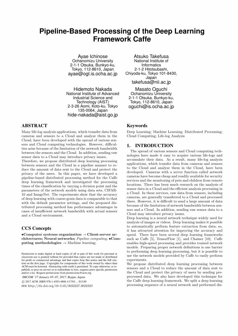
filters and changing the network bandwidth between the twomachines from 1 Gbps to 10 Mbps.Figures 16, 17 and 18 show the results of distibution1, set-ting the number of filters of the conv1 layer to 96, 72 and 48,respectively and Figures 19, 20 and 21 show the results ofdistibution2, setting the number of filters of the conv2 layerto 256, 192 and 128, respectively.

In both experiments, the results of case (3) are faster thanthose of the other cases when the network bandwidth be-tween two machines is 1 Gbps. However, it is confirmedthat for 10 Mbps and 50 Mbps, the results of case (3) takelonger than those of case (2) because the raw data are large,and it takes a longer time for communication, so the totalprocessing time is longer. In addition, the processing timein the distributed processing can be further reduced by re-ducing the number of filters. When the network bandwidthbetween the two machines is set to 10 Mbps, the result of

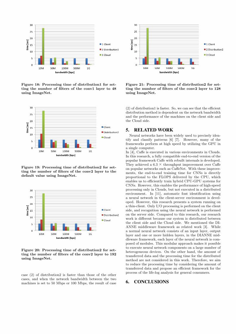
Figure 18: Processing time of distribution1 for set-ting the number of filters of the conv1 layer to 48using ImageNet.

Figure 19: Processing time of distribution2 for set-ting the number of filters of the conv2 layer to thedefault value using ImageNet.

Figure 20: Processing time of distribution2 for set-ting the number of filters of the conv2 layer to 192using ImageNet.

case (2) of distribution2 is faster than those of the othercases, and when the network bandwidth between the twomachines is set to 50 Mbps or 100 Mbps, the result of case

Figure 21: Processing time of distribution2 for set-ting the number of filters of the conv2 layer to 128using ImageNet.

(2) of distribution1 is faster. So, we can see that the efficientdistribution method is dependent on the network bandwidthand the performance of the machines on the client side andthe Cloud side.

5. RELATED WORKNeural networks have been widely used to precisely iden-

tify and classify patterns [6] [7]. However, many of theframeworks perform at high speed by utilizing the GPU ina single computer.In [4], Caffe is executed in various environments in Clouds.In this research, a fully compatible end-to-end version of thepopular framework Caffe with rebuilt internals is developed.They achieved a 6.3× throughput improvement over Caffeon popular networks such as CaffeNet. With these improve-ments, the end-to-end training time for CNNs is directlyproportional to the FLOPS delivered by the CPU, whichenables us to efficiently train hybrid CPU-GPU systems forCNNs. However, this enables the performance of high-speedprocessing only in Clouds, but not executed in a distributedenvironment. In [11], automatic font identification usinga neural network in the client-server environment is devel-oped. However, this research presents a system running ona thin-client. Only I/O processing is performed on the clientside, and recognition using the neural network is performedon the server side. Compared to this research, our researchwork is different because our system is distributed betweenthe client side and the Cloud side. We mentioned the DI-ANNE middleware framework as related work [3]. Whilea normal neural network consists of an input layer, outputlayer and one or more hidden layers, in the DIANNE mid-dleware framework, each layer of the neural network is com-posed of modules. This modular approach makes it possibleto execute neural network components on a large number ofheterogeneous devices. On the other hand, the amount oftransferred data and the processing time for the distributedmethod are not considered in this work. Therefore, we aimto reduce the processing time by considering the amount oftransferred data and propose an efficient framework for theprocess of the life-log analysis for general consumers.

6. CONCLUSIONS

We propose a pipeline-based distributed processing fordeep learning and implement the distributed processing ofthe deep learning framework Caffe for the purpose of thesensor data analysis process, considering privacy and thenetwork bandwidth. When we take into account a realisticnetwork bandwidth between general homes and a Cloud, ittakes time to transfer raw sensor data, so the effectivenessof the proposed method is proven. We observed that it ispossible to maintain a high accuracy and perform efficientprocessing even if we reduce the amount of transferred datafrom a sensor to a Cloud by reducing the number of filtersof the convolution layers.In the future, we will perform sexperiments using machinesof realistic performance as a client for general homes andusing video data.

7. ACKNOWLEDGMENTThis paper is partially based on results obtained from

a project commissioned by the New Energy and IndustrialTechnology Development Organization (NEDO) and JSPSKAKENHI Grant Number JP16K00177.

8. REFERENCES[1] M. Abadi, A. Agarwal, P. Barham, E. Brevdo,

Z. Chen, C. Citro, G. S. Corrado, A. Davis, J. Dean,M. Devin, S. Ghemawat, I. Goodfellow, A. Harp,G. Irving, M. Isard, Y. Jia, R. Jozefowicz, L. Kaiser,M. Kudlur, J. Levenberg, D. Mane, R. Monga,S. Moore, D. Murray, C. Olah, M. Schuster, J. Shlens,B. Steiner, I. Sutskever, K. Talwar, P. Tucker,V. Vanhoucke, V. Vasudevan, F. Viegas, O. Vinyals,P. Warden, M. Wattenberg, M. Wicke, Y. Yu, andX. Zheng. TensorFlow: Large-scale machine learningon heterogeneous systems, 2015. http://download.tensorflow.org/paper/whitepaper2015.pdf.pp. 1-19.

[2] K. Alex, V. Nair, and G. Hinton. The cifar-10 dataset.https://www.cs.toronto.edu/˜kriz/cifar.html(accessedDecember 27, 2015).

[3] E. De Coninck, T. Verbelen, B. Vankeirsbilck,S. Bohez, S. Leroux, and P. Simoens. Dianne:Distributed artificial neural networks for the internetof things. In In Proceedings of the 2Nd Workshop onMiddleware for Context-Aware Applications in the

IoT, M4IoT 2015, pages 19–24, New York, NY, USA,2015. ACM.

[4] S. Hadjis, F. Abuzaid, C. Zhang, and C. Re. Caffe controll: Shallow ideas to speed up deep learning. InProceedings of the Fourth Workshop on Data Analyticsin the Cloud, DanaC’15, pages 2:1–2:4, 2015.

[5] Y. Jia, E. Shelhamer, J. Donahue, S. Karayev,J. Long, R. Girshick, S. Guadarrama, and T. Darrell.Caffe: Convolutional architecture for fast featureembedding. In Proceedings of the 22Nd ACMInternational Conference on Multimedia (MM’14),pages 675–678, 2014.

[6] A. Krizhevsky, I. Sutskever, and G. E. Hinton.Imagenet classification with deep convolutional neuralnetworks. In F. Pereira, C. J. C. Burges, L. Bottou,and K. Q. Weinberger, editors, Advances in NeuralInformation Processing Systems 25, pages 1097–1105.2012.

[7] S. Pierre, E. David, Z. Xiang, M. Michael, F. Rob, andL. Yann. Overfeat: Integrated recognition, localizationand detection using convolutional networks. In InProceedings of International Conference on LearningRepresentations, 2013. 15 pages.

[8] O. Russakovsky, J. Deng, H. Su, J. Krause,S. Satheesh, S. Ma, Z. Huang, A. Karpathy,A. Khosla, M. Bernstein, A. C. Berg, and L. Fei-Fei.ImageNet Large Scale Visual Recognition Challenge.International Journal of Computer Vision (IJCV),115(3):211–252, 2015.

[9] R. Takano, T. Kudoh, Y. Kodama, and F. Okazaki.High-resolution timer-based packet pacing mechanismon linux operating system. IEICE Transactions onCommunications, E94.B(8):2199–2207, 2011.

[10] S. Tokui, K. Oono, S. Hido, and J. Clayton. Chainer:a next-generation open source framework for deeplearning. In In Proceedings of Workshop on MachineLearning Systems (LearningSys) in The Twenty-ninthAnnual Conference on Neural Information ProcessingSystems (NIPS), 2015. 6 pages.

[11] Z. Wang, J. Yang, H. Jin, J. Brandt, A. Agarwala,Z. Wang, Y. Song, J. Hsieh, E. Shechtman, S. Kong,and T. S. Huang. Deepfont: A system for fontrecognition and similarity. In In Proceedings of the23rd ACM international conference on Multimedia