Pipe Mapping with Monocular Fisheye Imagery

Peter Hansen, Hatem Alismail, Peter Rander and Brett Browning

Abstract— We present a vision-based mapping and localiza-tion system for operations in pipes such as those found inLiquified Natural Gas (LNG) production. A forward facingfisheye camera mounted on a prototype robot collects imageryas it is tele-operated through a pipe network. The imagesare processed offline to estimate camera pose and sparsescene structure where the results can be used to generate 3Drenderings of the pipe surface. The method extends state ofthe art visual odometry and mapping for fisheye systems toincorporate geometric constraints based on prior knowledgeof the pipe components into a Sparse Bundle Adjustmentframework. These constraints significantly reduce inaccuraciesresulting from the limited spatial resolution of the fisheyeimagery, limited image texture, and visual aliasing. Preliminaryresults are presented for datasets collected in our fiberglass pipenetwork which demonstrate the validity of the approach.

I. INTRODUCTIONPipe inspection is a critical task to a number of industries,

including Natural Gas production where pipe surface struc-ture changes at the scale of millimeters are of concern. Inthis work, we report on the development of a fisheye visualodometry and mapping system for an in-pipe inspectionrobot (e.g. [1]) to produce detailed, millimeter resolution3D surface structure and appearance maps. By registeringmaps over time, changes in structure and appearance canbe identified, which are both cues for corrosion detection.Moreover, these maps can be imported into rendering enginesfor effective visualization or measurement and analysis.

In prior work [2], we developed a verged perspectivestereo system capable of measuring accurate camera poseand producing dense sub-millimeter resolution maps. A limi-tation of the system was the inability of the camera to imagethe entire inner surface of the pipe. Here, we address thisissue by using a forward-facing wide-angle fisheye cameramounted on a small robot platform, as shown in Fig. 1a.This configuration enables the entire inner circumference tobe imaged from which full coverage appearance maps can beproduced. Fig. 1b shows the constructed 400mm (16 inch)internal diameter pipe network used in the experiments. Thispipe diameter is commonly used in Liquified Natural Gas(LNG) processing facilities, which is a target domain for oursystem. Sample images from the fisheye camera are shownin Figs. 1c and 1d. The extreme lighting variations evident inthe sample images pose significant challenges during imageprocessing, as discussed in Section III.

This publication was made possible by NPRP grant #08-589-2-245 fromthe Qatar National Research Fund (a member of Qatar Foundation). Thestatements made herein are solely the responsibility of the authors.

Hansen is with the QRI8 lab, Carnegie Mellon University, Doha, Qatarphansen@qatar.cmu.edu. Alismail, Rander, and Browning arewith the Robotics Institute/NREC, Carnegie Mellon University, PittsburghPA, USA, {halismai,rander,brettb}@cs.cmu.edu

(a) Robot. (b) Test pipe network.

(c) Image in straight section. (d) Image in T-intersection.

Fig. 1: The prototype robot with forward facing fisheyecamera (a), 400mm (16 inch) internal diameter pipe network(b), and sample images logged in a straight section (c) andT-intersection (d) during tele-operation through the network.Lighting is provided by 8 LEDs surrounding the camera.

Our system builds from established visual odometry andmultiple view techniques for central projection cameras [3],[4], [5], [6]. Binary thresholding, morphology and shapestatistics are first used to classify straight sections and T-intersection. Pose and structure results are obtained foreach straight section using a sliding window Sparse Bun-dle Adjustment (SBA) and localized straight cylinder fit-ting/regularization within the window. Fitting a new straightcylinder each window allows some degree of gradual pipecurvature to be modeled, e.g. sag in the pipes. After pro-cessing each straight section, results for the T-intersectionsare obtained using SBA and a two cylinder intersectionfitting/regularization – the two cylinders are the appropriatestraight sections of the pipe network. When applicable, loopclosure with g2o [7] is implemented using pose estimatesfrom visual correspondences in overlapping sections of adataset. As a final step, the pose and structure estimates areused to produce a dense point cloud rendering of the interiorsurface of the pipe network.

Results are presented in Section IV which show the visualodometry and sparse scene reconstruction for two datasetscollected in our pipe network. Dense 3D point cloud ren-derings for one dataset are also provided. These preliminaryresults illustrate the validity of the proposed system.

II. FISHEYE CAMERA

We use a 190◦ angle of view Fujinon fisheye lens fitted toa 1280pix× 960pix resolution CCD firewire camera. Imageformation is modeled using a central projection polynomialmapping, which is a common selection for fisheye cameras(e.g. [8], [9]). A scene point Xi projects to a coordinateη(θ, φ) = Xi/||Xi|| on the camera’s unit view spherecentered at the single effective viewpoint (0, 0, 0)T . Theangles θ and φ are, respectively, colatitude and longitude.The projected fisheye image coordinates u(u, v) are

u =

[(k1θ + k2θ

3 + k3θ4 + k4θ

5) cosφ+ u0(k1θ + k2θ

3 + k3θ4 + k4θ

5) sinφ+ v0

], (1)

where u0(u0, v0) is the principal point. Multiple imagesof a checkerboard calibration target with known Euclideangeometry were collected, and the model parameters fittedusing a non-linear minimization of the sum of squaredcheckerboard grid point image reprojection errors.

III. VISUAL ODOMETRY AND MAPPING

The visual odometry (VO) and mapping procedure isbriefly summarized as follows:A. Perform feature matching/tracking with keyframing.B. Divide images into straight sections and T-intersections.C. Obtain VO/structure estimates for each straight section

using a sliding window SBA and localized straight cylin-der fitting/regularization.

D. Obtain VO/structure estimates for each T-intersectionusing a two cylinder T-intersection model. This stepeffectively merges the appropriate straight sections.

E. Perform loop closure when applicable.The visual odometry steps (C and D) use different cylinder

fitting constraints to obtain scene structure errors includedas a regularization error in SBA. As previously mentioned,we have observed this to be a critically important stepwhich significantly improves the robustness and accuracy ofthe visual odometry and scene reconstruction estimates inthe presence of: limited spatial resolution from the fisheyecamera; feature location noise due to limited image textureand extreme lighting variations; and an often high percentageof feature tracking outliers due again to limited image textureand visual aliasing. At present an average a priori metricmeasurement of the pipe radius r is used during cylinderfitting. Cylinder fitting with a supplied pipe radius alsoresolves monocular visual odometry scale ambiguity.

A. Feature Tracking

An efficient region-based Harris detector [10] based on theimplementation in [6] is used to find a uniform feature distri-bution in each image. The image is divided into 2×2 regions,and the strongest N = 200 features per region are retained.Initial temporal correspondences between two images, imagei and image j, are found using cosine similarity matchingof 11 × 11 grayscale template descriptors for each feature.Each of these 11 × 11 template descriptors is interpolatedfrom a 31 × 31 region surrounding the feature. Five-pointrelative pose [3] and RANSAC [11] are used to remove

Fig. 2: Sparse optical flow vectors in a straight section (left)and T-intersection (right) obtained using a combination ofHarris feature matching and epipolar guided ZNCC.

outliers and provide an initial estimate of the essential matrixE. We experimented with multiple scale-invariant feature de-tectors/descriptors (e.g. SIFT [12], SURF [13]), but observedno significant improvements in matching performance.

For all unmatched features in image i, a guided Zero-mean Normalized Cross Correlation (ZNCC) is applied tofind their pixel coordinate in image j. Here, guided refersto a search within an epipolar region in image j. Sincewe implement ZNCC in the original fisheye imagery, weback project each integer pixel coordinate to a sphericalcoordinate η, and constrain the epipolar search regions using|ηT

j E ηi| < thresh — the subscripts denote image i and j.As a final step we implement image keyframing, selectingonly images separated by a minimum median sparse opticalflow magnitude or minimum percentage correspondences.Both minimums are selected empirically.

Fig. 2 shows examples of the sparse optical flow vectorsfor the feature correspondences found between keyframes ina straight section, and keyframes in a T-intersection. Featuresare ‘tracked’ across multiple frames by recursively matchingusing the method described.

The grayscale intensity of an imaged region of the pipesurface can change significantly between frames. This is dueprimarily to the non-uniform ambient lighting provided bythe robot. The cosine similarity metric for matching templatedescriptors and ZNCC were both selected to provide someinvariance to these intensity changes.

B. Image classification: straight vs. T-intersection

The image keyframes must be divided into straight sec-tions and T-intersection before implementing pose estimatingand mapping. To classify each image as belonging to astraight section or T-intersection, the image resolution isfirst reduced by sub-sampling pixels from every second rowand column. A binary thresholding is applied to extractdark blobs within the cameras field of view, followed bybinary erosion and clustering of the blobs. The largest blob isselected and the second moments of area L and Lp computedabout the blob centroid and principal point, respectively. Animage is classified as straight if the ratio Lp/L is less thanan empirical threshold; we expect to see a large round blobnear the center of images in straight sections.

Figs. 3a through 3c show the blobs extracted in threesample images, and initial classification of each image. After

(a) Straight section (b) T-intersection (c) T-intersection

0 500 1000 1500 2000 2500

Non−straight

Straight

Keyframe Number

0 500 1000 1500 2000 2500

Non−straight

Straight

Keyframe Number

(d) Initial classification (top), and after temporal filtering (bottom). Each ofthe 4 T-intersection clusters is a unique T-intersection in the pipe network.

Fig. 3: Straight section and T-intersection image classifica-tion. Example initial classifications (a-c), and the classifica-tion of all keyframes before and after temporal filtering (d).

initial classification, a temporal filtering is used to correctmis-classification, as illustrated in Fig. 3d. This filteringenforces a minimum straight/T-intersection cluster size.

C. Straight VO: Sliding Window SBA / local straight cylinder

For each new keyframe, the feature correspondences areused to estimate the new camera pose and scene pointscoordinates. This includes using Nister’s 5-point algorithmto obtain an initial unit-magnitude pose change estimate,optimal triangulation to reconstruct the scene points [4], andprior reconstructed scene coordinates in the straight sectionto resolve relative scale. After every 50 keyframes, a mod-ified sliding window SBA is implemented which includes alocalized straight cylinder fitting used to compute a scenepoint regularization error. A 100 keyframe window size isused which, for a typical dataset, equates to a segment ofpipe approximately one meter in length. This SBA is a multi-objective least squares minimization of image reprojectionerrors εI and scene point errors εX. An optimal estimate ofthe camera poses P and scene points X in the window, aswell as the fitted cylinder C are found which minimize thecombined error ε:

ε = εI + τ εX. (2)

The parameter τ is a scalar weighting which controls thetrade-off between the competing error terms εI and εX.

The image reprojection error εI is the sum of squareddifferences between all valid feature observations u andreprojected scene point coordinates u′:

εI =∑i

||ui − u′i||2, (3)

where u(u, v) and u′(u′, v′) are both inhomogeneous fisheyeimage coordinates.

The scene point error term εX is the sum of squared errorsbetween the optimized scene point coordinates X and a fitted

straight cylinder. The cylinder pose C is defined relative tothe first camera pose Pm = [Rm|tm] in the sliding windowas the origin. It is parameterized using 4 degrees of freedom:

C = [R | t]= [RX(γ)RY (β) | (tX , tY , 0)T ], (4)

where RA denotes a rotation about the axis A, and tA denotesa translation in the axis A. Each scene point coordinate Xi

maps to a coordinate Xi in the cylinder frame using

Xi = R (RmXi + tm) + t. (5)

The regularization error εX is

εX =∑i

(√X2

i + Y 2i − r

)2

, (6)

where the pipe radius r is supplied. Referring to (2), we usean empirically selected value τ = 2.5× 105.

As noted previously, there are frequently many featurecorrespondence outliers resulting from the challenging rawimagery. To minimize the influence of outliers, a Huberweighting is applied to individual error terms before comput-ing εI and εX. Outliers are also removed at multiple stages(iteration steps) using Median Absolute Deviation of the setof all signed Huber weighted errors u − u′. This outlierremoval stage is beneficial when the percentage of outliersis large.

D. T-intersections

The general procedure for processing the T-intersectionsis illustrated in Fig. 4. After processing each straight section,straight cylinders are fitted to the scene points in the first andlast 1 meter segment (Fig. 4a). In both cases, these cylindersare fitted with respect to the first and last camera poses asthe origins, respectively, using the parameterization in (4).

As illustrated in Fig. 4b, a T-intersection is modeled as twointersecting straight cylinders; the red cylinder axis intersectsthe blue cylinder axis at a unique point I. Let Pr be thefirst/last camera pose in a red section, and Cr be the cylinderfitted with respect to this camera as the origin. Similarly,let Pb be the last/first camera pose in a blue section, andCb be the cylinder fitted with respect to this camera as theorigin. The parameters ζr and ζb are rotations about the axisof the red and blue cylinders, and lr and lb are the signeddistances of the cylinder origins O(Cr) and O(Cb) from theintersection point I. Finally, φ is the angle of intersectionbetween the two cylinder axes in the range 0◦ ≤ φ < 180◦.These parameters fully define the change in pose Q betweenPb and Pr, and ensure that the two cylinder axes intersect ata single unique point I. Letting

D = p([RZ(ζr)|(0, 0, lr)T ], [RZ(ζb)RY (φ)|(0, 0, lb)T ]

),

(7)where p(b, a) is a projection a followed by b, and RA is arotation about axis A, then

Q = p (inv(Cr), p(D,Cb)) , (8)

where inv(Cr) is the inverse projection of Cr.

(a) Straight sections with cylinders fitted to endpoints.

(b) The two cylinder T-intersectionmodel parameters (refer to text fordetailed description). The red andblue cylinders have the same inter-nal radius r and are constrained tointersect at a unique point I.

(c) Visual odometry and scene re-construction result using the T-intersection model. The scene pointshave been automatically assigned toeach cylinder allowing cylinder fitregularization terms to be evaluated.

Fig. 4: A T-intersection is modeled as the intersection ofcylinders fitted to the straight sections of the pipe. Respec-tively, the blue and red colors distinguish the horizontal andvertical sections of the ‘T’, as illustrated in (b).

SBA is used to optimize all camera poses PT in the T-intersection between Pr and Pb, as well as all new scenepoints X in the T-intersection, and the T-intersection modelparameters Φ(ζr, lr, ζb, lb, φ). Again, the objective functionminimized is the same form as (2), which includes an imagereprojection error (3) and scene fitting error (6). The samevalue τ = 2.5×105, robust cost function, and outlier removalscheme are also used.

Special care needs to be taken when computing the scenefitting error εX in (6) as there are two cylinders Cr, Cb

in the T-intersection model. Specifically, we need to assigneach scene point to one of the cylinders, and compute theindividual error terms in (6) with respect to this cylinder.This cylinder assignment is performed by finding the distanceto each of the cylinder surfaces, and selecting the cylinderfor which the absolute distance is a minimum. Fig. 4cshows the results for one of the T-intersections after SBAhas converged. The color-coding of the scene points (dots)represent their cylinder assignment.

E. Loop Closure

For multi-loop datasets, loop closure is implemented usingthe graph based optimization algorithm g2o [7]. The graphvertices are the set of all camera poses described by their Eu-clidean coordinates and orientations (quaternions). The graphedges connect temporally adjacent camera poses, and theloop closures connecting camera poses in the same sectionof the pipe network visited at different times. Each edge has

Fig. 5: Pipe network: T1 through T4 are the T-intersections.

an associated relative pose estimate between the vertices itconnects, and a covariance of the estimate. Alternate graph-based loop closure techniques with comparable performanceand improved efficiency could also be used (e.g. [14]).

Our constrained environment enables potential loop clo-sures to be selected without the need for visual placerecognition techniques, such as those based on bag of visualwords (BoW)[15]. This is achieved by knowing the sectionof the network where the robot begins, and simply countingleft/right turns – see Fig. 5. Let Pi and Pj be the poses inthe same straight section of pipe visited at different times.We compute the Euclidean distances li and lj to the T-intersection centroid I at the end of the straight section.Poses Pi are Pj are selected as a candidate pair if li ≈ lj .

Once candidate loop closure poses Pi ↔ Pj are se-lected, the relative pose estimate is refined using imagecorrespondences found by matching SIFT descriptors forthe previously detected Harris corners. SIFT descriptors areused at this stage to achieve improved rotation invariance.Prior knowledge of the surrounding scene structure (fittedcylinders) is used to resolve the monocular scale ambiguityof the relative pose estimates obtained using the five-pointalgorithm and RANSAC, followed by non-linear refinement.

IV. EXPERIMENTS AND RESULTSTwo grayscale monocular fisheye image datasets

(1280pix× 960pix resolution, 7.5 frames per second) werecollected in our constructed 400mm (16 inch) internaldiameter fiberglass pipe network shown in Fig. 5. Forthis, the robot was tele-operated using images streamedover a wireless link, and all lighting was provided by8 high intensity LEDs equipped on the robot — seeFig. 1. Dataset A is a near full loop of the pipe networkcontaining approximately 26,000 images, from which 2760keyframes were automatically selected. Dataset B is a fullloop datasets containing approximately 24,000 images and4170 keyframes. All image processing steps described inSection III were implemented offline.

A. Visual Odometry

The visual odometry and sparse scene reconstruction re-sults for each straight section in dataset A were shownpreviously in Fig. 4a. The complete results for both datasetsare provided in Fig. 6. The labels T1 through T4 correspondto those in Fig. 5. Note that no loop closure was possiblefor dataset A. For dataset B, loop closure was implementedusing 15 loop closure poses in the straight section betweenthe T-intersections T1 and T4.

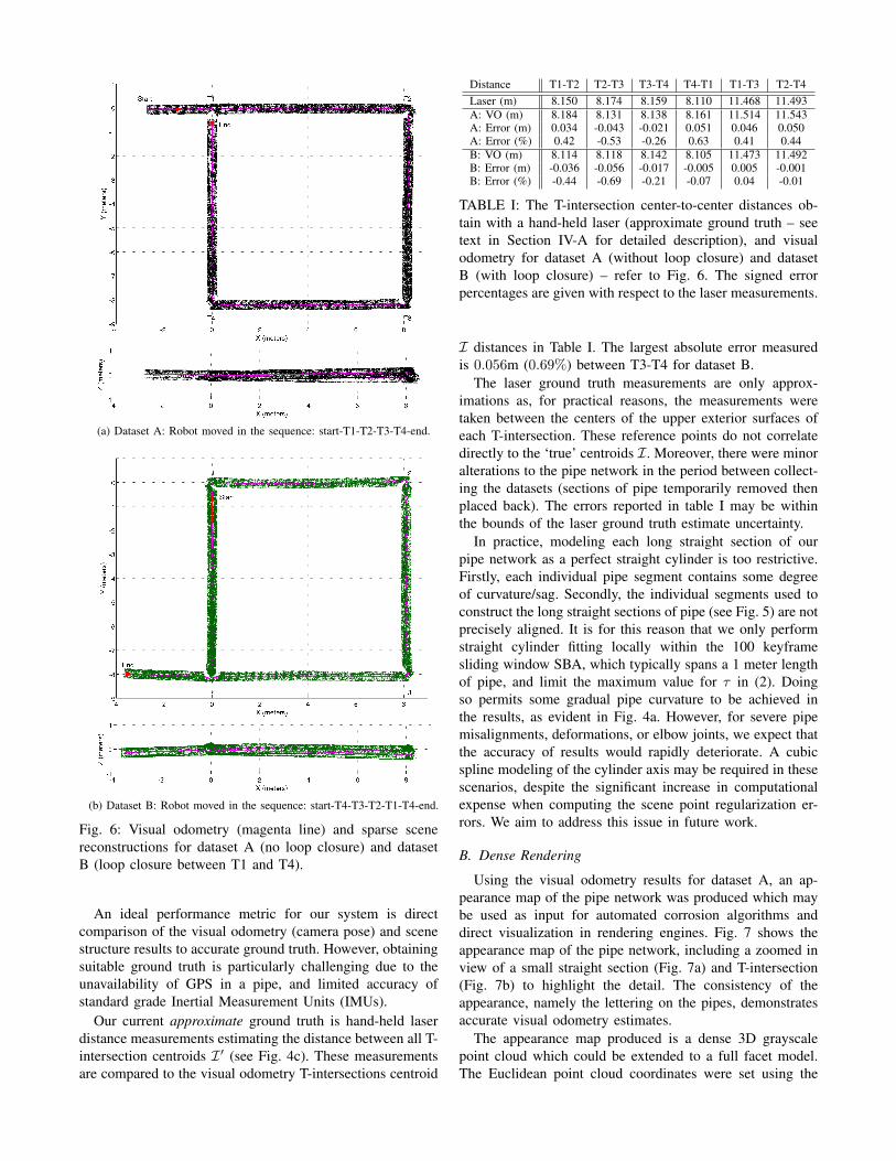
(a) Dataset A: Robot moved in the sequence: start-T1-T2-T3-T4-end.

(b) Dataset B: Robot moved in the sequence: start-T4-T3-T2-T1-T4-end.

Fig. 6: Visual odometry (magenta line) and sparse scenereconstructions for dataset A (no loop closure) and datasetB (loop closure between T1 and T4).

An ideal performance metric for our system is directcomparison of the visual odometry (camera pose) and scenestructure results to accurate ground truth. However, obtainingsuitable ground truth is particularly challenging due to theunavailability of GPS in a pipe, and limited accuracy ofstandard grade Inertial Measurement Units (IMUs).

Our current approximate ground truth is hand-held laserdistance measurements estimating the distance between all T-intersection centroids I ′ (see Fig. 4c). These measurementsare compared to the visual odometry T-intersections centroid

Distance T1-T2 T2-T3 T3-T4 T4-T1 T1-T3 T2-T4Laser (m) 8.150 8.174 8.159 8.110 11.468 11.493A: VO (m) 8.184 8.131 8.138 8.161 11.514 11.543A: Error (m) 0.034 -0.043 -0.021 0.051 0.046 0.050A: Error (%) 0.42 -0.53 -0.26 0.63 0.41 0.44B: VO (m) 8.114 8.118 8.142 8.105 11.473 11.492B: Error (m) -0.036 -0.056 -0.017 -0.005 0.005 -0.001B: Error (%) -0.44 -0.69 -0.21 -0.07 0.04 -0.01

TABLE I: The T-intersection center-to-center distances ob-tain with a hand-held laser (approximate ground truth – seetext in Section IV-A for detailed description), and visualodometry for dataset A (without loop closure) and datasetB (with loop closure) – refer to Fig. 6. The signed errorpercentages are given with respect to the laser measurements.

I distances in Table I. The largest absolute error measuredis 0.056m (0.69%) between T3-T4 for dataset B.

The laser ground truth measurements are only approx-imations as, for practical reasons, the measurements weretaken between the centers of the upper exterior surfaces ofeach T-intersection. These reference points do not correlatedirectly to the ‘true’ centroids I. Moreover, there were minoralterations to the pipe network in the period between collect-ing the datasets (sections of pipe temporarily removed thenplaced back). The errors reported in table I may be withinthe bounds of the laser ground truth estimate uncertainty.

In practice, modeling each long straight section of ourpipe network as a perfect straight cylinder is too restrictive.Firstly, each individual pipe segment contains some degreeof curvature/sag. Secondly, the individual segments used toconstruct the long straight sections of pipe (see Fig. 5) are notprecisely aligned. It is for this reason that we only performstraight cylinder fitting locally within the 100 keyframesliding window SBA, which typically spans a 1 meter lengthof pipe, and limit the maximum value for τ in (2). Doingso permits some gradual pipe curvature to be achieved inthe results, as evident in Fig. 4a. However, for severe pipemisalignments, deformations, or elbow joints, we expect thatthe accuracy of results would rapidly deteriorate. A cubicspline modeling of the cylinder axis may be required in thesescenarios, despite the significant increase in computationalexpense when computing the scene point regularization er-rors. We aim to address this issue in future work.

B. Dense Rendering

Using the visual odometry results for dataset A, an ap-pearance map of the pipe network was produced which maybe used as input for automated corrosion algorithms anddirect visualization in rendering engines. Fig. 7 shows theappearance map of the pipe network, including a zoomed inview of a small straight section (Fig. 7a) and T-intersection(Fig. 7b) to highlight the detail. The consistency of theappearance, namely the lettering on the pipes, demonstratesaccurate visual odometry estimates.

The appearance map produced is a dense 3D grayscalepoint cloud which could be extended to a full facet model.The Euclidean point cloud coordinates were set using the

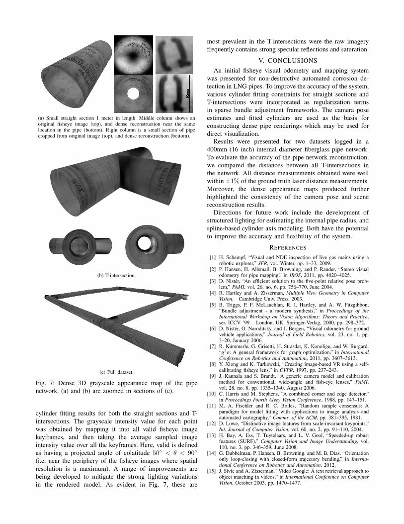
(a) Small straight section 1 meter in length. Middle column shows anoriginal fisheye image (top), and dense reconstruction near the samelocation in the pipe (bottom). Right column is a small section of pipecropped from original image (top), and dense reconstruction (bottom).

(b) T-intersection.

(c) Full dataset.

Fig. 7: Dense 3D grayscale appearance map of the pipenetwork. (a) and (b) are zoomed in sections of (c).

cylinder fitting results for both the straight sections and T-intersections. The grayscale intensity value for each pointwas obtained by mapping it into all valid fisheye imagekeyframes, and then taking the average sampled imageintensity value over all the keyframes. Here, valid is definedas having a projected angle of colatitude 50◦ < θ < 90◦

(i.e. near the periphery of the fisheye images where spatialresolution is a maximum). A range of improvements arebeing developed to mitigate the strong lighting variationsin the rendered model. As evident in Fig. 7, these are

most prevalent in the T-intersections were the raw imageryfrequently contains strong specular reflections and saturation.

V. CONCLUSIONSAn initial fisheye visual odometry and mapping system

was presented for non-destructive automated corrosion de-tection in LNG pipes. To improve the accuracy of the system,various cylinder fitting constraints for straight sections andT-intersections were incorporated as regularization termsin sparse bundle adjustment frameworks. The camera poseestimates and fitted cylinders are used as the basis forconstructing dense pipe renderings which may be used fordirect visualization.

Results were presented for two datasets logged in a400mm (16 inch) internal diameter fiberglass pipe network.To evaluate the accuracy of the pipe network reconstruction,we compared the distances between all T-intersections inthe network. All distance measurements obtained were wellwithin ±1% of the ground truth laser distance measurements.Moreover, the dense appearance maps produced furtherhighlighted the consistency of the camera pose and scenereconstruction results.

Directions for future work include the development ofstructured lighting for estimating the internal pipe radius, andspline-based cylinder axis modeling. Both have the potentialto improve the accuracy and flexibility of the system.

REFERENCES

[1] H. Schempf, “Visual and NDE inspection of live gas mains using arobotic explorer,” JFR, vol. Winter, pp. 1–33, 2009.

[2] P. Hansen, H. Alismail, B. Browning, and P. Rander, “Stereo visualodometry for pipe mapping,” in IROS, 2011, pp. 4020–4025.

[3] D. Nister, “An efficient solution to the five-point relative pose prob-lem,” PAMI, vol. 26, no. 6, pp. 756–770, June 2004.

[4] R. Hartley and A. Zisserman, Multiple View Geometry in ComputerVision. Cambridge Univ. Press, 2003.

[5] B. Triggs, P. F. McLauchlan, R. I. Hartley, and A. W. Fitzgibbon,“Bundle adjustment - a modern synthesis,” in Proceedings of theInternational Workshop on Vision Algorithms: Theory and Practice,ser. ICCV ’99. London, UK: Springer-Verlag, 2000, pp. 298–372.

[6] D. Nister, O. Naroditsky, and J. Bergen, “Visual odometry for groundvehicle applications,” Journal of Field Robotics, vol. 23, no. 1, pp.3–20, January 2006.

[7] R. Kummerle, G. Grisetti, H. Strasdat, K. Konolige, and W. Burgard,“g2o: A general framework for graph optimization,” in InternationalConference on Robotics and Automation, 2011, pp. 3607–3613.

[8] Y. Xiong and K. Turkowski, “Creating image-based VR using a self-calibrating fisheye lens,” in CVPR, 1997, pp. 237–243.

[9] J. Kannala and S. Brandt, “A generic camera model and calibrationmethod for conventional, wide-angle and fish-eye lenses,” PAMI,vol. 28, no. 8, pp. 1335–1340, August 2006.

[10] C. Harris and M. Stephens, “A combined corner and edge detector,”in Proceedings Fourth Alvey Vision Conference, 1988, pp. 147–151.

[11] M. A. Fischler and R. C. Bolles, “Random sample consensus: Aparadigm for model fitting with applications to image analysis andautomated cartography,” Comms. of the ACM, pp. 381–395, 1981.

[12] D. Lowe, “Distinctive image features from scale-invariant keypoints,”Int. Journal of Computer Vision, vol. 60, no. 2, pp. 91–110, 2004.

[13] H. Bay, A. Ess, T. Tuytelaars, and L. V. Gool, “Speeded-up robustfeatures (SURF),” Computer Vision and Image Understanding, vol.110, no. 3, pp. 346–359, June 2008.

[14] G. Dubbelman, P. Hansen, B. Browning, and M. B. Dias, “Orientationonly loop-closing with closed-form trajectory bending,” in Interna-tional Conference on Robotics and Automation, 2012.

[15] J. Sivic and A. Zisserman, “Video Google: A text retrieval approach toobject matching in videos,” in International Conference on ComputerVision, October 2003, pp. 1470–1477.