PIPE FLOW - fkm.utm.mysyahruls/resources/SKMM1313/8-Pipe.pdf · The overall head loss for the pipe...

Chapter 8 – Pipe Flow

PIPE FLOW

The Energy Equation The first law of thermodynamics for a system is, in words Net time rate of

energy addition by work transfer into

the system

= + Time rate of

energy of the

Net time rate of energy addition by heat transfer into

the system

increase of the total storage

t We could express this relation by using Bernoulli equation as :

lossininin

outoutout hz

gV

gP

zg

VgP

+++=++22

22

ρρ hloss head loss

1


EXAMPLE 1

Figure 1

A 30m wide river with a flowrate of 800m3/s flows over a rock pile as shown in Figure 1. Determine the direction of flow and the head loss associated with the flow across the rock pile.

2


EXAMPLE 2

Figure 2

An incompressible liquid flows steadily along the pipe shown in Figure 2. Determine the direction of flow and the head loss over the 6m length of pipe.

3


EXAMPLE 3

Figure 3

Water is pumped steadily through a 0.10m diameter pipe from one closed, pressurized tank to another as shown in Figure 3. The pump adds 4.0kW to the water and the head loss of the flow is 10m. Determine the velocity of the water leaving the pipe.

4


EXAMPLE 4

Figure 4

Water flows through a vertical pipe as shown in Figure 4. Is the flow up or down? Explain.

5


PIPE FLOW

General Characteristic of Pipe Flow

Figure 1

Some of the basic components of a typical pipe system are shown in Figure 1. They include the pipes, the various fitting used to connect the individual pipes to form the desired system, the flowrate control device or valves, and the pumps or turbines that add energy to or remove energy from the fluid.

1


(a) Pipe flow (b) Open-channel flow

Figure 2 The difference between open-channel flow and the pipe flow is in the fundamental mechanism that drives the flow. For open-channel flow, gravity alone is the driving force – the water flows down a hill. For pipe flow, gravity may be important (the pipe need not be horizontal), but the main driving force is likely to be a pressure gradient along the pipe. If the pipe is not full, it is not possible to maintain this pressure difference, P1- P2.

2


Laminar and Turbulent Flow

Figure 3

The flow of a fluid in a pipe may be laminar flow or it may be turbulent flow. Osborne Reynolds (1842-1912), a British scientist and mathematician, was the first to distinguish the difference between these two classifications of flow by experimental. For “small enough flowrates” the dye streak ( a streakline) will remain as a well-defined line as it flows along, with only slight blurring due to molecular diffusion of the dye into the surrounding water. It is called laminar flow.

3


For “intermediate flowrate” the dye streak fluctuates in time and space, and intermittent burst of irregular behavior appear along the streak. It is called transitional flow. For “large enough flowrates” the dye streak almost immediately becomes blurred and spreads across the entire pipe in a random fashion. It is called turbulent flow. To determine the flow conditions, one dimensionless parameter was introduced by Osborne Reynolds, called the Reynolds number, Re. Reynolds number, Re is the ratio of the inertia to viscous effects in the flow. It is written as ;

µρVD

=Re ρ : Density (kg/m3) V : Average velocity in pipe (m/s) D : Diameter of pipe (m) µ : Dynamic viscosity (Ns/m2)

The distinction between laminar and turbulent pipe flow and its dependence on an appropriate dimensionless quantity was first appointed out by Osborne Reynolds in 1883.

4


The Reynolds number ranges for which laminar, transitional or turbulent pipe flows are obtained cannot be precisely given. The actual transition from laminar to turbulent flow may take place at various Reynolds numbers, depending on how much the flow is disturbed by vibration of pipe, roughness of the entrance region and other factors. For general engineering purpose, the following values are appropriate : 1. The flow in a round pipe is laminar if the Reynolds

number is less than approximately 2100. 2. The flow in a round pipe is turbulent if the

Reynolds numbers is greater that approximately 4000.

3. For Reynolds number between these two limits, the flow may switch between laminar and turbulent conditions in an apparently random fashion.

5


Entrance Region and Fully Developed Laminar Flow

Figure 4 The region of flow near where the fluid enters the pipe is termed the entrance region. The shape of velocity profile in the pipe depends on whether the flow is laminar or turbulent, as does the length of the entrance region, el

6


The dimensionless entrance length, Del , correlates quite well with the Reynolds number. Typical entrance lengths are given by ;

(Re06.0=D

el ) (for laminar flow) and

( )61

Re4.4=D

el (for turbulent flow) for Re=2000, De 120=l

for 104<Re<105, DD e 3020 << l From figure 4, the flow between (2) and (3) is termed fully developed flow.

7


Fully Developed Turbulent Flow

Figure 5

Turbulent in pipe flow is actually more likely to occur than laminar flow in practical situation. Turbulent flow is a very complex process.

8


For pipe flow the value of the Reynolds number must be greater than approximately 4000 for turbulent flow. For flow along a flat plate the transition between laminar and turbulent flow occurs at a Reynolds number of approximately 500,000.

µρVL

=plateflat Re

9


PIPE FLOW

Losses in Pipe It is often necessary to determine the head loss, hL, that occur in a pipe flow so that the energy equation, can be used in the analysis of pipe flow problems. The overall head loss for the pipe system consists of the head loss due to viscous effects in the straight pipes, termed the major loss and denoted hL-major. The head loss in various pipe components, termed the minor loss and denoted hL-minor. That is ;

hL = hL-major + hL-minor The head loss designations of “major” and “minor” do not necessarily reflect the relative importance of each type of loss. For a pipe system that contains many components and a relatively short length of pipe, the minor loss may actually be larger than the major loss.

1


Major Losses The head loss, hL-major is given as ;

gV

Dfh majorL 2

2l=−

where f is friction factor. Above mention equation is called the Darcy-Weisbach equation. It is valid for any fully developed, steady, incompressible pipe flow, whether the pipe is horizontal or on hill Friction factor for laminar flow is ;

Re64

=f Friction factor for turbulent flow is based on Moody chart. It is because, in turbulent flow, Reynolds number and relative roughness influence the friction.

Reynolds number, µρVD

=Re

Relative roughness Dε

= (relative roughness is not present in the laminar flow)

2


3


The Moody chart is universally valid for all steady, fully developed, incompressible pipe flows. The following equation from Colebrook is valid for the entire non-laminar range of the Moody chart. It is called Colebrook formula.

⎟⎟

⎠

⎞

⎜⎜

⎝

⎛+−=

fD

f Re51.2

7.3log0.21 ε

4


Minor Losses The additional components such as valves and bend add to the overall head loss of the system, which is turn alters the losses associated with the flow through the valves. Minor losses termed as ;

gV

Kh LL 2

2

minor =−

where KL is the loss coefficient. Each geometry of pipe entrance has an associated loss coefficient.

5


Entrance flow conditions and loss coefficient.

Condition: 02

1 =AA

or ∞=2

1

AA

6


Exit flow conditions and loss coefficient.

Condition: 02

1 =AA

or ∞=2

1

AA

7


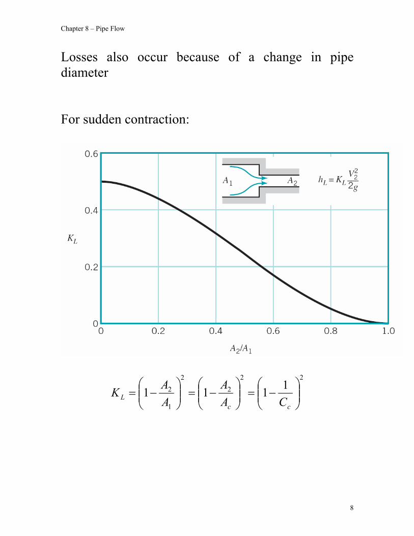
Losses also occur because of a change in pipe diameter For sudden contraction:

22

2

2

1

2 1111 ⎟⎟⎠

⎞⎜⎜⎝

⎛−=⎟⎟

⎠

⎞⎜⎜⎝

⎛−=⎟⎟

⎠

⎞⎜⎜⎝

⎛−=

ccL CA

AAA

K

8


For sudden expansion

2

2

11 ⎟⎟⎠

⎞⎜⎜⎝

⎛−=

AA

K L

9


EXAMPLE 1

Figure 1 Water flows from the nozzle attached to the spray tank shown in Figure 1. Determine the flowrate if the loss coefficient for the nozzle (based on upstream conditions) is 0.75 and the friction factor for the rough hose is 0.11.

10


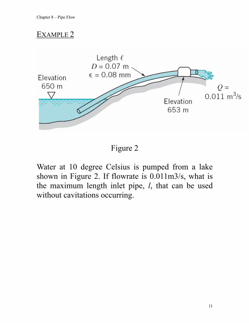
EXAMPLE 2

Figure 2

Water at 10 degree Celsius is pumped from a lake shown in Figure 2. If flowrate is 0.011m3/s, what is the maximum length inlet pipe, l, that can be used without cavitations occurring.

11


EXAMPLE 3

Figure 3 Water flows steadily through the 2.5cm diameter galvanized iron pipe system shown in Figure 3 at rate 6x10-4m3/s. Your boss suggests that friction losses in the straight pipe sections are negligible compared to losses in the threaded elbows and fittings of the system. Do you agree or disagree with your boss? Support your answer with appropriate calculations.

12


13


PIPE FLOW A pipe system which has only one pipe line is called single pipe system. In many pipe systems there is more than one pipe line involved, and this mechanism is called multiple pipe systems. Multiple pipe systems are the same as for the single pipe system; however, because of the numerous unknowns involved, additional complexities may arise in solving for the flow in these systems.

Single pipe system

Multiple pipe systems

1


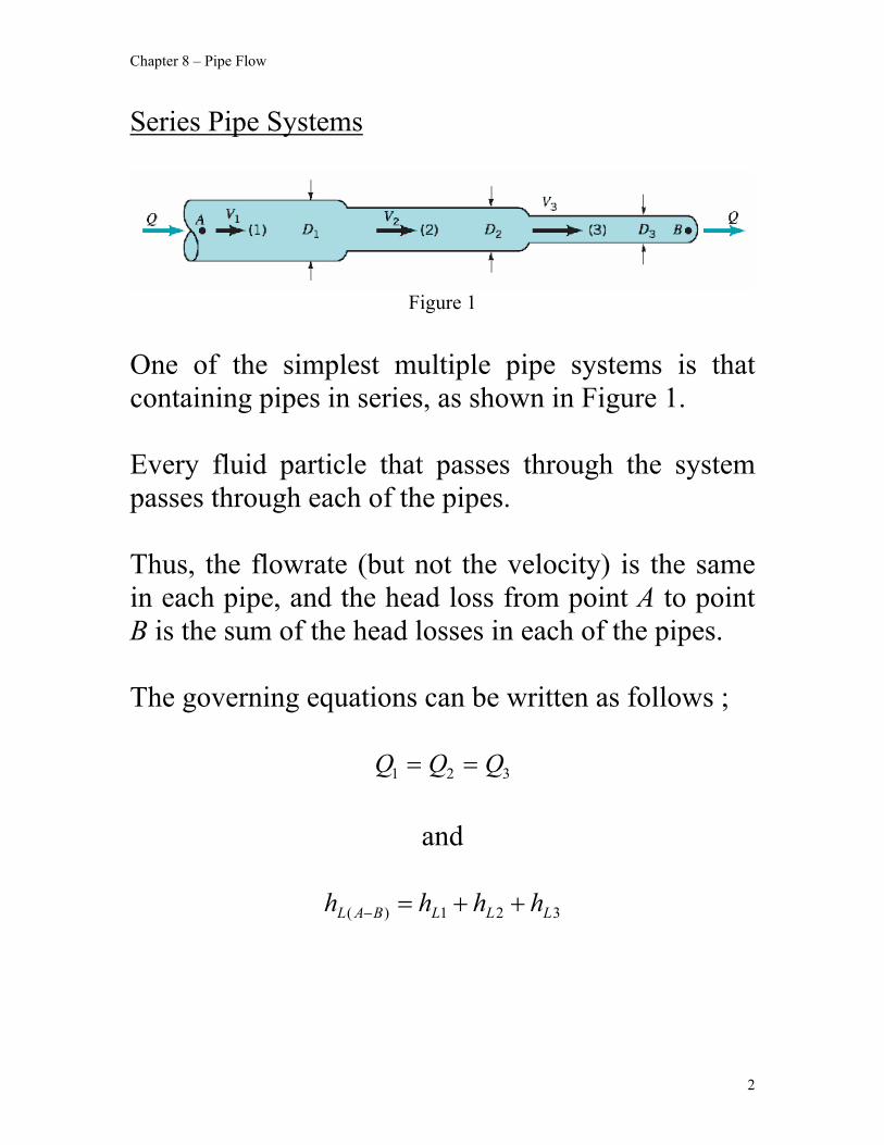
Series Pipe Systems

Figure 1

One of the simplest multiple pipe systems is that containing pipes in series, as shown in Figure 1. Every fluid particle that passes through the system passes through each of the pipes. Thus, the flowrate (but not the velocity) is the same in each pipe, and the head loss from point A to point B is the sum of the head losses in each of the pipes. The governing equations can be written as follows ;

321 QQQ ==

and

321)( LLLBAL hhhh ++=−

2


Parallel Pipe Systems

Figure 2

Another common multiple pipe system contains pipes in parallel, as shown in Figure 2. In this system a fluid particle traveling from A to B may take any of paths available, with the total flowrate equal to the sum of the flowrates in each pipe. The head loss experienced by any fluid particle traveling between these two locations is independent of the path taken. The governing equation for parallel pipe systems are ;

321 QQQQ ++=

and

321 LLL hhh ==

3


Loop Pipe Systems

Figure 3

Another type of pipe system called a loop is shown in Figure 3. In this case, the flowrate through pipe (1) equals the sum of the flowrates through pipes (2) and (3), or

321 QQQ +=

The energy equation between the surfaces of each reservoir, the head loss for pipe (2) must equal that for pipe (3), even though the pipe sizes and flowrates may be different for each.

4


For a fluid particle traveling through pipe (1) and (2):

21

22

22 LLBBB

AAA hhz

gV

gPz

gV

gP

++++=++ρρ

For a fluid particle traveling through pipe (1) and (3):

31

22

22 LLBBB

AAA hhz

gV

gPz

gV

gP

++++=++ρρ

These can be combined to give :

32 LL hh =

5


Three-reservoir system

Figure 4 The branching system termed the three-reservoir problem shown in Figure 4. With all valves open, however, it is not necessarily obvious which direction the fluid flows. According to Figure 4, it is clear that fluid flows from reservoir A because the other reservoir levels are lower.

6


EXAMPLE 1 Air flows in a 0.5m diameter pipe at a rate of 10m3/s. The pipe diameter changes to 0.75m through a sudden expansion. Determine the pressure rise across this expansion. Explain how there can be a pressure rise across the expansion when there is an energy loss (KL > 0) EXAMPLE 2 The surface elevations of reservoir A, B and C are at 640m, 545m and 580m respectively. A 0.45m diameter pipe, 3.2km long runs from reservoir A to a node at an elevation of 610m, where the 0.3m diameter pipes each of 1.6km length branch from the original pipe and connect reservoirs B and C. If the friction factor for each pipe is 0.020, determine the flowrate in each pipe.

7


EXAMPLE 3

Figure 5 The three water-filled tanks shown in Figure 5 are connected by pipes as indicated. If minor losses are neglected, determine the flowrate in each pipe.

8


TUTORIAL 1 FOR PIPE FLOW

Question 1 Carbon dioxide at 20ºC and a pressure of 550 kPa(abs) flows in a pipe at a rate of 0.04N/s. Determine the maximum diameter allowed if the flow is to be turbulent. Question 2 A soft drink with the properties of 10ºC water is sucked through a 4mm diameter, 0.25m long straw at a rate of 4cm3/s. Is the flow at the outlet of the straw laminar? Is it fully developed? Explain. Question 3 Water flow in a constant diameter pipe with the following conditions measured: At section (a); Pa=22.5kPa and za=17m. At section (b); Pb=20kPa and zb=21m. Is the flow from (a) to (b) or from (b) to (a)? Explain.

1


PAST YEAR QUESTION FOR PIPE FLOW

Question 1 Rajah 1 menunjukkan satu aliran dalam paip licin yang dikawal oleh tekanan udara di dalam tangki. Berapakah tekanan tolok (pressure gauge) P1 yang diperlukan supaya air yang mempunyai ketumpatan dan kelikatan masing-masing ialah 998 kg/m3 dan 1.003x10-3 kg/m.s mengalir dengan kadar 60 m3/jam. Ambil pekali kehilangan pada pengecilan dan bengkokkan pada paip masing-masing 0.5 dan 0.4.

Rajah 1

1


Question 2 a) Terangkan apakah yang dimaksudkan dengan kehilangan besar (major loss) dan

kehilangan kecil (minor loss) untuk suatu system paip. b) Sebuah system paip keluli komersil seperti yang dilakarkan dalam Rajah 2 digunakan

untuk mengepam bendalir penyejukkan yang berketumpatan bandingan 0.92 dan berkelikatan dinamik 1.7577x10-4 Pa.s dari tangki B ke tangki A. Jika kadar aliran bendalir penyejukkan yang dipam ke tangki A ialah 140 liter per minit pada keadaan injap terbuka sepenuhnya, tentukan kuasa pam untuk memastikan aras cecair penyejukkan di dalam tangki A dan B kekal pada aras seperti yang dilakarkan dalam rajah. Semua dimensi dalam gambarajah adalah dalam unit meter (m).

Rajah 2

2


Question 3 a) Explain the physical meaning of Reynolds number. b) Water is pumped at the rate of 60 liters per second from a reservoir to free discharge

shown in Figure 3. All pipes are made of commercial steel. Determine the power required by the pump if the efficiency of the pump is 85%. Included all the losses in the pipe system. Moody diagram is given. Viscosity of water is given as 1x10-3 Pa.s.

Figure 3

3

PIPE FLOW - fkm.utm.mysyahruls/resources/SKMM1313/8-Pipe.pdf · The overall head loss for the pipe...

Documents

Transcript of PIPE FLOW - fkm.utm.mysyahruls/resources/SKMM1313/8-Pipe.pdf · The overall head loss for the pipe...