Pillars of Heaven

6th International Conference on High Energy Density Laboratory AstrophysicsMarch 11 – 14, 2006

Marc Pound University of Maryland

Jave Kane, Bruce Remington, Dmitri RyutovLawrence Livermore National Laboratory

Akira MizutaMax-Planck-Institute for Astrophysics

How do pillars form?

Pillars (elephant trunks) common

Formation mechanism unclear

Instabilities at cloud interface?

Pre-existing dense cores?

Observations of morphology alonecannot distinguish between models.

H+

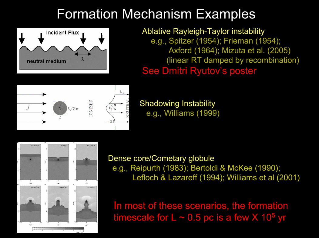
Formation Mechanism ExamplesAblative Rayleigh-Taylor instability

e.g., Spitzer (1954); Frieman (1954); Axford (1964); Mizuta et al. (2005)

(linear RT damped by recombination)See Dmitri Ryutov’s poster

Shadowing Instabilitye.g., Williams (1999)

Dense core/Cometary globulee.g., Reipurth (1983); Bertoldi & McKee (1990);

Lefloch & Lazareff (1994); Williams et al (2001)

In most of these scenarios, the formationtimescale for L ~ 0.5 pc is a few X 105 yr

Measure received power W as a function of frequency; Antenna temperature TA= W/k. Doppler shift gives radial velocity.

θ ~ 0.2 – 10'' δV ~ 0.1 km/s

CO(J=1–0) is the primary observational surrogate for H2

Horsehead Nebula

0.5 pc

Radiotelescopes

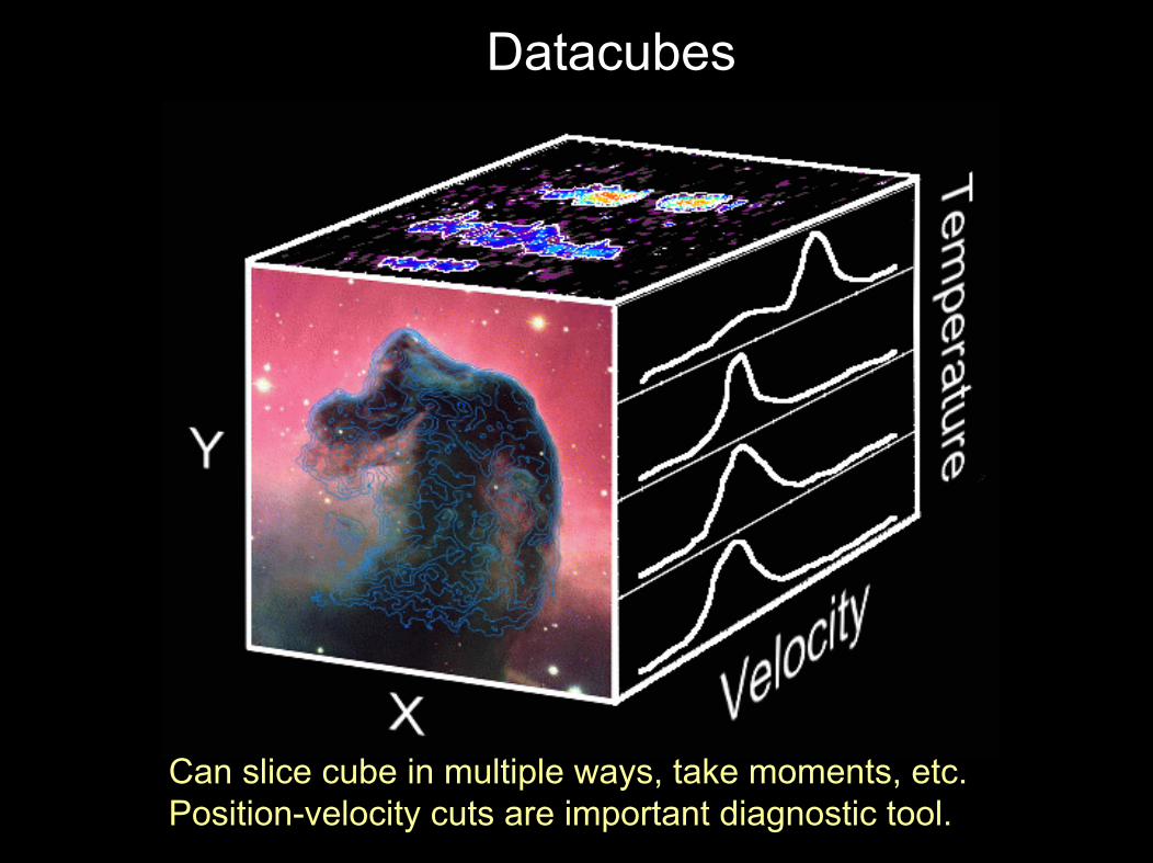
Datacubes

Can slice cube in multiple ways, take moments, etc.Position-velocity cuts are important diagnostic tool.

Geometry of Eagle Nebula

Pillars are also inclined to line of sight

CO(J=1-0) Integrated Intensity

Our Data from BIMA radio interferometer

What the observations tell us (model constraints)

Observables

Temperature

Velocity

absolute

gradient

dispersion

line shape

Magnetic Field

Derivables

Density

Mass

Pressure

thermal

turbulent

Column density

Timescales:

Dynamical

Evaporation

... 40 K

... 25 km/s

... 2-10 km/s/pc

... 1 km/s

... complex

... ??

... 105 cm-3

... 800 Msun

(dyne cm-2)... 10-10

... 10-8

... 1022 cm-2

... 105 years

... 107 years

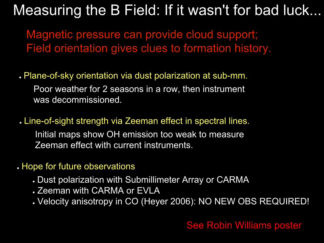
See Robin Williams poster

Measuring the B Field: If it wasn't for bad luck...Magnetic pressure can provide cloud support; Field orientation gives clues to formation history.

● Hope for future observations

● Plane-of-sky orientation via dust polarization at sub-mm.

● Line-of-sight strength via Zeeman effect in spectral lines.

Poor weather for 2 seasons in a row, then instrument was decommissioned.

Initial maps show OH emission too weak to measureZeeman effect with current instruments.

● Dust polarization with Submillimeter Array or CARMA● Zeeman with CARMA or EVLA● Velocity anisotropy in CO (Heyer 2006): NO NEW OBS REQUIRED!

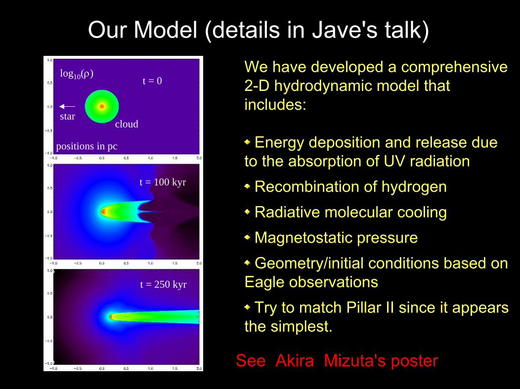
Our Model (details in Jave's talk)We have developed a comprehensive 2-D hydrodynamic model that includes:

Energy deposition and release due to the absorption of UV radiation

Recombination of hydrogenRadiative molecular coolingMagnetostatic pressureGeometry/initial conditions based on

Eagle observationsTry to match Pillar II since it appears

the simplest.

See Akira Mizuta's poster

log10(ρ)

starcloud

positions in pc

t = 0

t = 100 kyr

t = 250 kyr

The Objective To go from this...

R, Z, VR, VZ, ρ...to this.

X, Y, VZ, F

We need to create synthetic observations (datacube)by ''observing'' the model. (See my last HEDLA talk)

Synthetic Observations – very briefly

BIMA millimeter array

Interferometers measure the Fourier Transform of the sky brightness distributionAs Earth rotates, antennas pairs trace out ellipses in the Fourier domain, sampling different spatial frequencies. Longer baselines give higher spatial resolution. Orient model on sky to match Eagle. Sample it with the same uv coverage. FFT and deconvolveusing the known point spread function. u

v

Example uv coverage

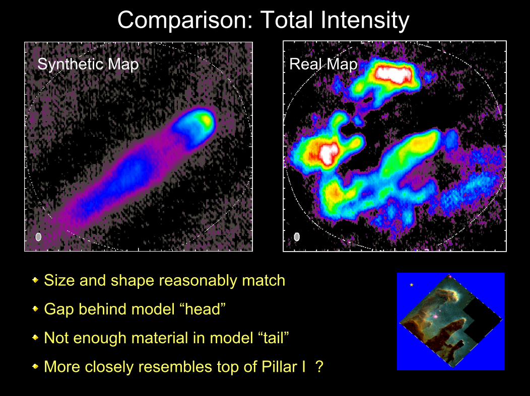
Comparison: Total Intensity

Size and shape reasonably match

Gap behind model “head”

Not enough material in model “tail”

More closely resembles top of Pillar I ?

Synthetic Map Real Map

Location of Position-Velocity Cuts

Synthetic Map Real Map

Comparison: Velocity Field (Long axis)

Velocity gradient is roughly correct. Not enough material in model tail. Velocity dispersion too small in model (Line width too narrow).

5 km

/s

~ 1 pc

Comparison: Velocity Field (short axis)

Model shows signature of “inside-out shear”; data cut not so obvious.Model has limb brightening, data do not.

3 km

/s

~0.3 pc

My Ideal Scaled Laser Experiment

● Real molecular clouds have structure.

● Velocity, velocity, velocity!Measure pillar internal velocities with spectrometer or VISAR

See Paula Rosen’s poster

M ~ 10

Re ~ 5x108

Clumps, filaments, inter-clump gas

My Ideal Scaled Laser Experiment

● Real molecular clouds have structure.

● Velocity, velocity, velocity!Measure pillar internal velocities with spectrometer or VISAR

See Paula Rosen’s poster

M ~ 10

Re ~ 5x108

Clumps, filaments, inter-clump gas

“The question you need to ask yourself is Do I feel lucky?”

My Ideal Scaled Laser Experiment

● Real molecular clouds have structure.

● Velocity, velocity, velocity!Measure pillar internal velocities with spectrometer or VISAR

See Paula Rosen’s poster

M ~ 10

Re ~ 5x108

“Well, do ya, punk?

Clumps, filaments, inter-clump gas

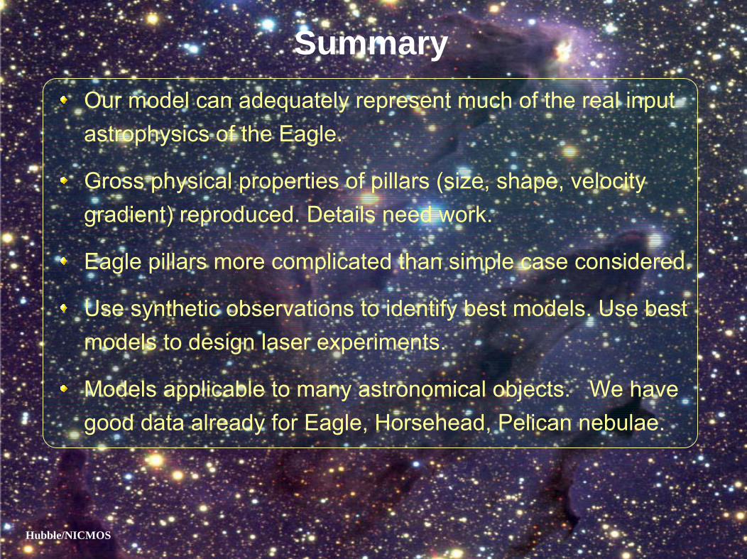
Summary Our model can adequately represent much of the real input astrophysics of the Eagle.

Gross physical properties of pillars (size, shape, velocity gradient) reproduced. Details need work.

Eagle pillars more complicated than simple case considered.

Use synthetic observations to identify best models. Use best models to design laser experiments.

Models applicable to many astronomical objects. We have good data already for Eagle, Horsehead, Pelican nebulae.

Hubble/NICMOS

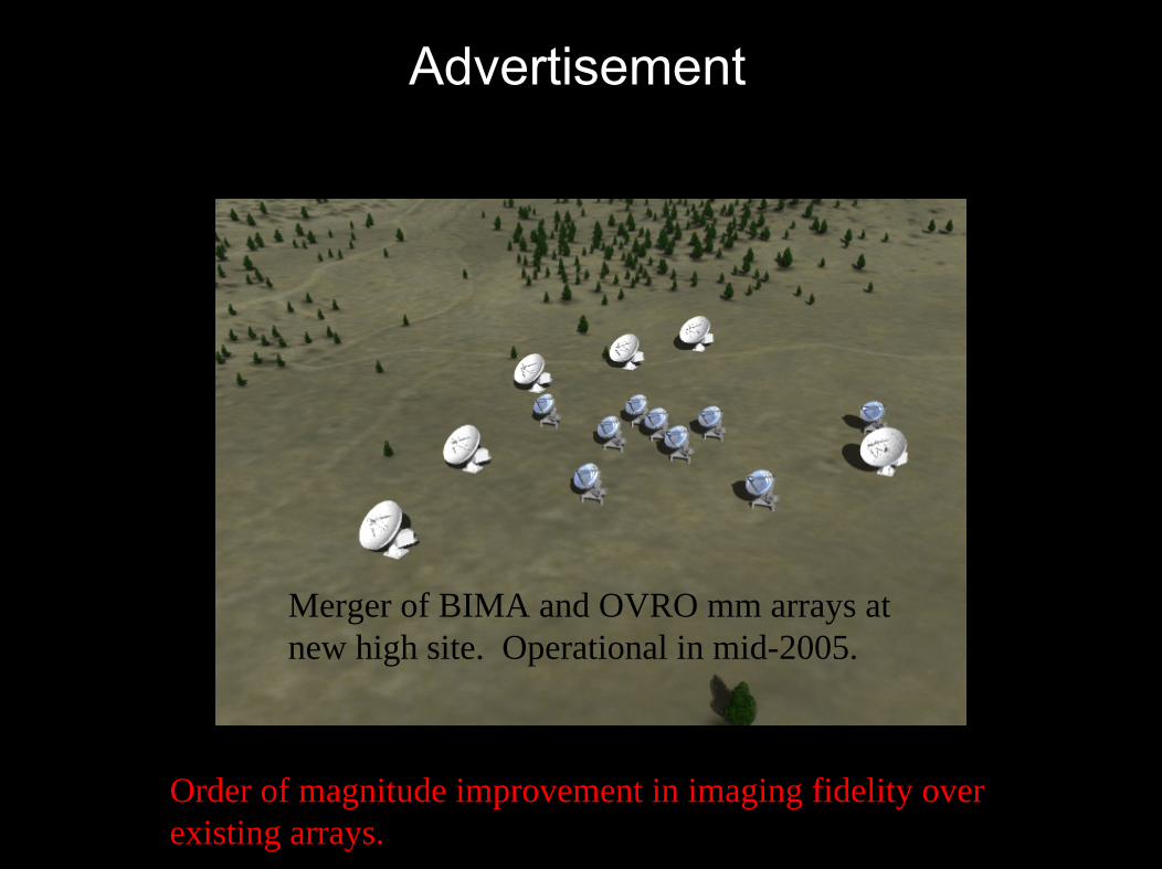
AdvertisementThe Combined Array for Research in Millimeter-wave Astronomy

(CARMA)

Merger of BIMA and OVRO mm arrays atnew high site. Operational in mid-2005.

Order of magnitude improvement in imaging fidelity over existing arrays.

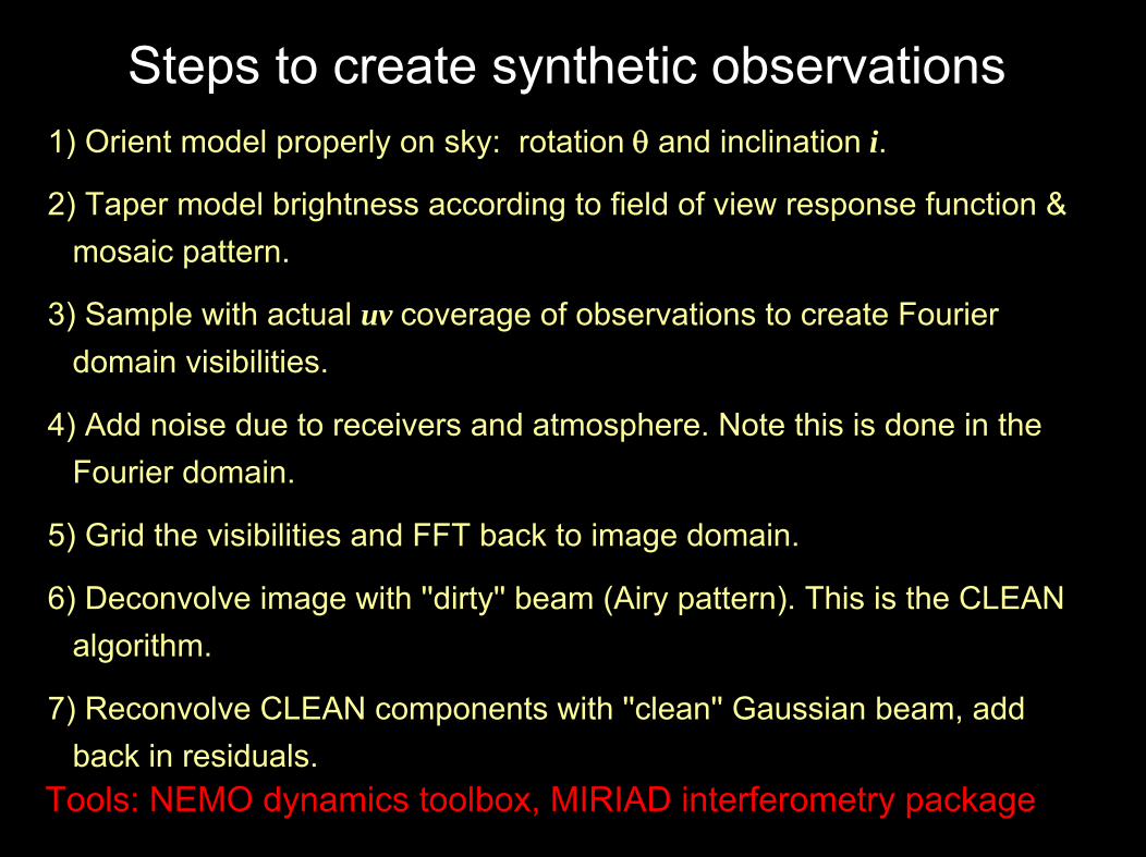
Steps to create synthetic observations1) Orient model properly on sky: rotation θ and inclination i.

2) Taper model brightness according to field of view response function & mosaic pattern.

3) Sample with actual uv coverage of observations to create Fourier domain visibilities.

4) Add noise due to receivers and atmosphere. Note this is done in the Fourier domain.

5) Grid the visibilities and FFT back to image domain.

6) Deconvolve image with ''dirty'' beam (Airy pattern). This is the CLEAN algorithm.

7) Reconvolve CLEAN components with ''clean'' Gaussian beam, add back in residuals.

Tools: NEMO dynamics toolbox, MIRIAD interferometry package

SuccessesBasic shape reproduced

Correct final densities reproduced:

n(H2) = 103 – 105 cm-3

Correct velocity gradient reproduced:

VY sini ~ 3 km/s/pc, compare with 2.2 km/s/pc in Pillar II

CaveatsNo radiative transfer – brightness assumed proportional to mass in pixel.Comparing 2D model to integrated 3D datacube – need a full 3D or cylindrical model to examine velocity field and pillar substructure.

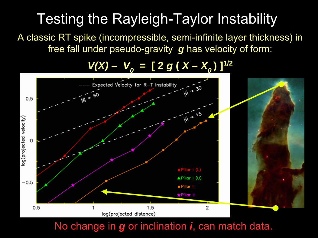
Testing the Rayleigh-Taylor Instability

No change in g or inclination i, can match data.

A classic RT spike (incompressible, semi-infinite layer thickness) in free fall under pseudo-gravity g has velocity of form:

V(X) – V0 = [ 2 g ( X – X0 ) ]1/2

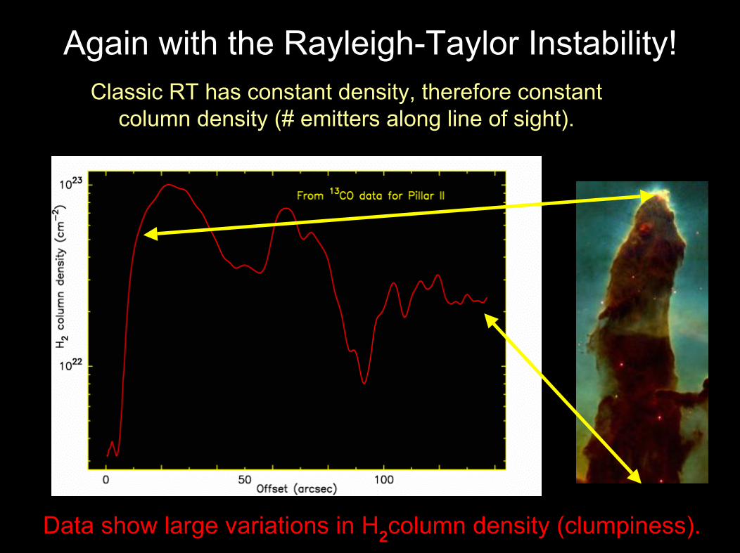
Again with the Rayleigh-Taylor Instability!Classic RT has constant density, therefore constant

column density (# emitters along line of sight).

Data show large variations in H2column density (clumpiness).

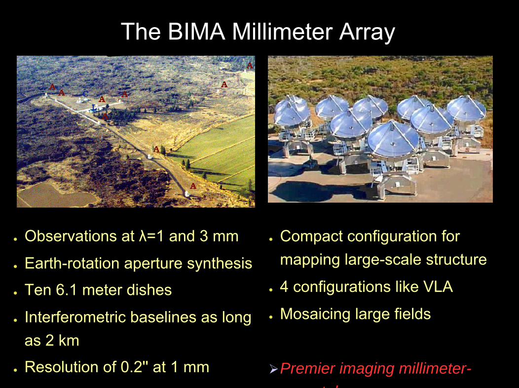
The BIMA Millimeter Array

● Observations at λ=1 and 3 mm

● Earth-rotation aperture synthesis

● Ten 6.1 meter dishes

● Interferometric baselines as long as 2 km

● Resolution of 0.2'' at 1 mm

● Compact configuration for mapping large-scale structure

● 4 configurations like VLA

● Mosaicing large fields

Premier imaging millimeter-wave telescope

How long will the Horsehead last?

evaporation timescaletevap= M / (dM/dt)

mass loss rate due to photoionizationdM/dt = 2�r2 ci mpni

Lyman continuum absorbed in layer comparable to cloud radiusni = (LLyC / 4�αB)1/2 r-1/2 d-1

tevap ~ 5 Myr

...plug in the numbers, turn crank...

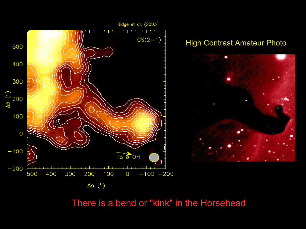
High Contrast Amateur Photo

There is a bend or "kink" in the Horsehead

Horsehead NebulaV = 8 – 15 km/s

CO(J=1-0) Integrated Intensity

Horsehead Nebula

Centroid Velocitycontours: 0.5 km/s

Velocity Dispersioncontours: 0.15 km/s

Molecular clouds

Agglomerations of molecular material with masses 102 to 106 Msun

Located primarily in galactic spiral arms

Where stars form

Dominated by turbulence

Clumpy structure

Temperatures ~ few X 10K

Volume densities ~ 103 – 107 cm-3

Primarily H2 with traces of:

CO – 10– 4

dust – 10– 2

Bell Labs

10 pc

Orion GMC

Complications

● Eagle pillars appear to be in a very late stage of RT evolution, after the bubble has burst.

● Horsehead appears to be in early stage, but nearby star formation history unclear.

● Magnetic fields