1

Piketty’s 𝑟 − 𝑔 model: wealth inequality and tax policy

Clemens Fuest†, Andreas Peichl

‡ and Daniel Waldenström

◊

February 20, 2015

Abstract

This study discusses implications of Piketty’s (2014) 𝑟 − 𝑔 model for wealth inequality and

tax policy. Using historical cross-country panel data on wealth inequality and indicators of

capital returns and income growth we find some tentative empirical support for the predic-

tions of the 𝑟 − 𝑔 model. The scope for addressing inequality by increasing taxes on capital is

limited due to capital mobility but some tax instruments, in particular recurrent taxes on im-

movable property, may offer an opportunity to tax the well off without undermining economic

growth. Our main conclusion, however, is that more research is needed to establish a clearer

understanding of the links between macroeconomic development and distributional outcomes.

JEL: D31, H20, N10

Keywords: r-g model, wealth distribution, tax policy, redistribution.

† ZEW (fuest@zew.de), University of Mannheim, CESifo and IZA.

‡ ZEW (peichl@zew.de), University of Mannheim, CESifo and IZA.

◊ Department of Economics, Uppsala University (daniel.waldenstrom@nek.uu.se), IZA, UCLS, UCFS, IFN and

IFAU.

2

1. Introduction

The so-called 𝑟 − 𝑔 model of Piketty (2014), which relates the difference between the rate of

return on capital, 𝑟, and the rate of income growth, 𝑔 to the level of economic inequality has

received enormous attention in both academic and popular circles. In its simplest characteriza-

tion, it says that when existing (“old”) capital grows faster than new capital is created out of

accumulated incomes, then already relatively rich capital owners will become even richer

relative to the others not holding capital, and thus inequality will increase. In Piketty (2014)

and Piketty and Zucman (2014, 2015) this model was incorporated into and derived from a

more general theoretical framework.

How convincing is the view that the difference between the return on capital and the rate of

economic growth is a key factor driving economic inequality? Piketty’s formula raises a num-

ber of theoretical and empirical issues. From a theoretical perspective it is clear 𝑟 > 𝑔 is nei-

ther necessary nor sufficient for inequality to increase. It is not necessary because inequality

may increase due to other reasons like, for instance, inequality of labour income, which has

been a key driver of the recent surge in income inequality in the United States. It is not suffi-

cient either, in particular because capitalists may earn much but save little. As recently em-

phasised by Mankiw (2015), 𝑟 > 𝑔 may not lead to increasing inequality because capital in-

come taxes may reduce the net return to capital below g or because capital owners consume

part of their income. If capital owners have enough children, wealth concentration will fall as

they leave their wealth to the next generation.1

In addition, even if capital owners save a lot their income cannot grow indefinitely. While the

interest rate may indeed be permanently higher than the growth rate of GDP, it is obvious that

capital income cannot permanently grow faster than GDP. Also, the marginal productivity

will decline as the capital intensity of production increases.

At the same time, while it is true that economic theory offers no unambiguous support for the

view that 𝑟 > 𝑔 leads to increasing inequality, it is equally true that a growing difference be-

tween 𝑟 and 𝑔 may, at least for periods of time, be an important factor driving income or

wealth inequality, as argued by Piketty (2014) and Piketty and Zucman (2014, 2015). How the

difference between 𝑟 and 𝑔 is related to inequality is ultimately an empirical question which

1 However, evidence suggests that the number of children is decreasing with income (Jones and Tertilt, 2006).

The average number of children per family is below 2 for rich households.

3

we address in this paper. We also derive implications for tax policy based on our empirical

findings.

2. The 𝒓 − 𝒈 model and wealth inequality: A preliminary empirical assessment

What is the empirical relationship between 𝑟 − 𝑔 and economic inequality? To date quite lim-

ited systematic evidence about this relationship has been presented. Piketty himself presents

some circumstantial pieces of evidence and informative point estimates in Piketty (2014), but

the book contains no comprehensive statistical analysis using detailed historical country-

specific or cross-country datasets. Recently, Acemoglu and Robinson (2015) made an attempt

to empirically assess the 𝑟 − 𝑔 model by relating proxies of 𝑟 − 𝑔 to top income shares and

the capital share of value added. Their main analysis used data from the World Top Income

Database to regress the annual level of top income shares against the annual level of 𝑟 − 𝑔

(including lags) and it did not indicate any clear systematic relationships. Acemoglu and Rob-

inson also could not establish a link when using up to 20-year averages or capital share of

value added as main inequality outcome.2 While their empirical results thus questioned the

mechanisms of the 𝑟 − 𝑔 model, Piketty (2015) pointed out a number of potential explana-

tions to their findings as well as conceptual problems with some of their data.

One important mechanism of the 𝑟 − 𝑔 model that was not examined by Acemoglu and Rob-

inson, however, is how 𝑟 − 𝑔 influences wealth inequality. Even if income inequality has

generally received more attention, the inequality of wealth is, in fact, at the centre of Piketty’s

𝑟 − 𝑔 model and perhaps the most direct distributional outcome of the 𝑟 − 𝑔 relationship.3

We will in this essay therefore present a preliminary analysis of the link between 𝑟 − 𝑔 and

some standard measures of wealth concentration. There are several challenges associated with

empirically estimating the 𝑟 − 𝑔 model for wealth inequality. First, we can think of no catch-

all measure of the rate of return to capital, 𝑟. For example, we know that 𝑟 varies between

different types of capital and we know that the composition of capital differs between coun-

tries, time periods and potentially also over the wealth distribution. Instead of trying to com-

2 Acemoglu and Robinson presented several variants of these regressions, but none of them suggested a system-

atic relationship between 𝑟 − 𝑔 and top income shares or the capital share. See also Piketty (2015) for a discus-

sion of their results. 3 See Piketty and Zucman (2015) and Piketty (2015) for a systematic derivation of this effect. In brief, they show

using different variants of dynamic wealth accumulation models that a higher 𝑟 − 𝑔 differential is associated

with a higher wealth inequality.

4

pute an explicit measure of 𝑟, which we know would be highly imperfect in most dimensions,

we therefore propose a proxy of 𝑟 being the development of the financial sector. Much of the

capital held by the rich consists of financial assets, either in the form of bank deposits, cash

and bonds, or as corporate stock.4 Therefore the growth of the financial sector, measured as a

combination of the size of the banking sector and stock market capitalization, may in fact cap-

ture much of what we want to capture as canonical 𝑟 in the 𝑟 − 𝑔 model. We do, however,

also run regressions similar to Acemoglu and Robinson (2015) where we assume 𝑟 to be the

same over time and across countries and only let the level of income growth 𝑔 vary. Needless

to say, all of these measures carry large problems of their own, but we leave it to future re-

search to dwell deeper into measuring and estimating these variables.

A second challenge concerns time horizons. The 𝑟 − 𝑔 model essentially describes the rela-

tionship between macroeconomic outcomes in steady state and is therefore not concerned

primarily with annual variation in the relevant outcomes. In our regressions, we therefore use

averages over five-year periods. We sometimes include lag variables stretching back three

five-year periods, i.e., 15 years. A third challenge is that wealth inequality is also not meas-

ured as consistently and abundantly measured as income inequality is measured. We use the

available data on historical top wealth shares that researchers have produced as of today,

yielding a dataset with at most nine countries spanning some 130 years in the longest case.5

Our econometric methodology is to regress the wealth share of the top percentile 𝑇𝑜𝑝𝑊1%

(“the rich”), the next nine percentiles in the top decile 𝑇𝑜𝑝𝑊10 − 1% (“the upper middle

class”), and the bottom nine deciles 𝐵𝑜𝑡𝑊90% (“the rest”), a highly heterogeneous group, on

a set of explanatory variables. Our most important explanatory variables are 𝑟, which is the

level of financial development (𝐹𝑖𝑛. 𝑑𝑒𝑣.) and its growth (�̃�), and 𝑔, which is measured as the

log GDP per capita in level (𝑌) and growth (𝑔). According to the 𝑟 − 𝑔 model, we would ex-

pect that a higher 𝑟 increases top wealth shares but reduces bottom wealth shares due to the

skewed distribution of capital possessions. Equivalently, we would expect that a higher 𝑔

reduces top wealth shares but increases bottom wealth shares, all according to the logic that

4 For example, Saez and Zucman (2014) find that about 90 percent of the wealth held by the U.S. top 0.1 wealth

percentile is different kinds of financial assets. 5 Our data are based a dataset constructed by Roine, Vlachos and Waldenström (2009) where variable definitions

and sources are provided. These data were recently updated and complemented with top wealth shares by the

Roine and Waldenström (2015) handbook chapter. For the U.S. top wealth shares we use the series of Saez and

Zucman (2014). The other countries included in this analysis are Argentina, Australia, Finland, Netherlands,

Norway, Sweden, Switzerland and the U.K.

5

higher income growth enables the less well-off to accumulate new wealth and thus reduce

wealth concentration. We also include control variables aimed at accounting for other influ-

ences on wealth concentration in order to see whether there are other, underlying institutional

political or economic variables, that drive both 𝑟 and 𝑔 and wealth concentration. Here we

include measures of income inequality, measured as the income shares to the top percent

(𝑇𝑜𝑝𝑌1%), next nine percent (𝑇𝑜𝑝𝑌10 − 1%) and the bottom nine deciles (𝐵𝑜𝑡𝑌90%), trade

openness measured as the sum of imports and exports as share of GDP (𝑂𝑝𝑒𝑛𝑛𝑒𝑠𝑠), two

measures of public-sector redistribution proxied by the size of central government spending

(𝐺𝑜𝑣. 𝑠𝑝𝑒𝑛𝑑.) and top marginal income taxation (𝑀𝑎𝑟𝑔𝑡𝑎𝑥), and a control for the country’s

population size (𝑃𝑜𝑝). The econometric specification follows the similar analysis of Roine,

Vlachos and Waldenström (2009) in which a first-difference GLS accounting for country-

specific effects and country-specific time trends was used in order to hold constant as many

unobserved influences as possible.

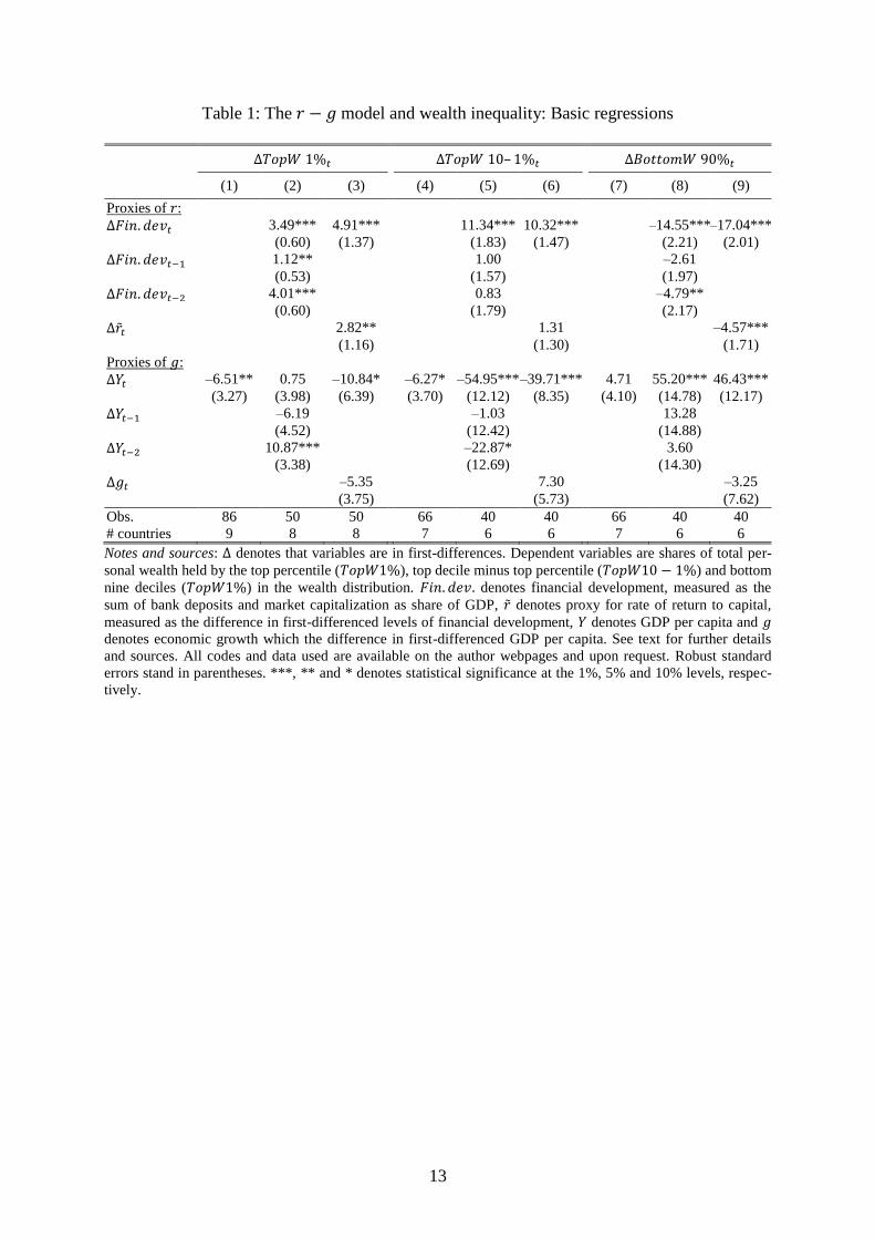
The results are presented in two tables. Table 1 shows stripped-down regressions where

wealth shares of the different groups are regressed on 𝑟 and 𝑔. Looking first at the impact of 𝑟

– whether in contemporaneous or lagged levels or growth – it is consistently positively asso-

ciated with higher wealth shares in the top percentile and the next nine percentiles of the top

decile (columns 1 through 6). For example, increasing total capitalization by one standard

deviation (0.5, about 50% of GDP) is related to an instant increase in the wealth share of the

top percentile by about 4 percentage points. When the lags are also included the increase is

almost 10 percentage points. As the mean wealth share of the top percentile is about 30 per-

cent, this effect is notable. The bottom nine percentiles in the wealth distribution, however,

experience the exact opposite effect, reduced wealth shares, following financial sector growth.

Looking instead at economic growth, 𝑔, the pattern is quite the opposite: a higher GDP per

capita growth is negatively associated with top wealth shares but positively associated with

bottom wealth shares. The impact is not as clear within the top as it is in the case of financial

development, in particular as concerns the actual growth variable g which is statistically in-

significant for all wealth groups.

[Table 1 about here]

Table 2 reports the 𝑟 − 𝑔 regressions when including controls for some institutional differ-

ences across countries. The general pattern from the regressions in Table 1 is still visible and,

6

in fact, stronger when adding controls for income inequality and other potentially important

confounding factors. The growth of the financial sector, our proxy for 𝑟, is positively correlat-

ed with top wealth shares, in particular the shares of the top percentile. By contrast, income

growth, 𝑔, is negatively associated with top wealth shares, once again most clearly visible in

the top percentile. As for the bottom 90 percent, admittedly a very heterogeneous group of

wealth holders, the signs are opposite, with wealth shares decreasing as the financial sector

expands but increasing as GDP per capital grows. The other control variables included in the

regressions are not of primary interest to us in this investigation, yet it is reassuring to note

that in particular public sector influence, whether in the form of government spending or mar-

ginal taxation of incomes, works in the expected direction by having a negative association

with top wealth shares. Income distribution seems, also not too unexpectedly, correlated with

the wealth distribution, especially in the top. But since incomes are themselves in part directly

determined by wealth (e.g., in the form of capital income), the interpretation of these simulta-

neous outcomes cannot be fully settled here.

Altogether, the results in Tables 1 and 2 offer some tentative support for the 𝑟 − 𝑔 model as

proposed by Piketty (2014) and its proposed links between the 𝑟 − 𝑔 differential and wealth

inequality. Given the considerable problems at hand with measurement, data availability and

statistical specification, much more effort is of course needed before we can begin to speak

about any stable relationships in these outcomes. Furthermore, the relationship between top

wealth shares, financial sector development and economic growth reveals nothing about the

direction of causality. For instance, it is perfectly possible that an increasing wealth concen-

tration causes a stronger growth of the financial sector. We conclude therefore that more re-

search is needed to settle the issues at hand.

[Table 2 about here]

3. Implications for Tax Policy

What are the policy implications of the results described in the preceding section? As pointed

out above the available empirical evidence is insufficient to conclude that the difference be-

tween 𝑟 and 𝑔 does indeed cause either income or wealth inequality. It is nevertheless inter-

esting to consider different policy options to address inequality in the light of the hypothesis

that 𝑟 − 𝑔 may be an important driver of inequality. Piketty (2014) argues that governments

7

should use tax policy to fight trends towards increasing inequality. He proposes that govern-

ments should levy higher taxes on capital income and wealth. The ambition is that higher tax-

es on capital income will reduce the after tax return to capital and thus tend to reduce ine-

quality of income and, ultimately, wealth. Wealth taxes would address wealth inequality di-

rectly. This proposal raises two questions: Firstly, how effective are capital taxes as an in-

strument to redistribute income, that is to reduce the (after tax) return on capital? Secondly,

what are the implications of this proposal for economic growth?

3.1 How effective are capital taxes as an instrument to redistribute income?

An important objection against using capital income taxes as an instrument for income redis-

tribution is that trying to do so will be self-defeating if capital is internationally mobile. High-

er taxes would just lead to capital outflows until the after tax rate of return is the same as be-

fore, and the burden of capital taxation would fall on domestic immobile factors of produc-

tion, in particular labour.6

This argument is most relevant for source-based capital income taxes. The most important

source-based capital tax in existing tax systems is the corporate income tax. Empirical work

on the impact of corporate income taxes on the international location of investment confirms

that corporate income taxes have a significant effect on investment behaviour. Countries with

a high income tax burden attract less investment and the investment they do attract is less

profitable (Becker et al., 2012). Governments have understood this and, in the last two dec-

ades, reduced their corporate income tax rates significantly.

There are two ways in which countries can try to avoid that higher domestic taxes on capital

income reduce domestic investment. Firstly, they can try to coordinate their tax policy inter-

nationally. This has been suggested many times in the past, with little effect, even within the

European Union. The main reason for this inability to coordinate is that different countries

have very different interests. While large countries with high income levels and preferences

for high tax rates and high levels of public expenditures typically favour international tax co-

ordination with the objective to limit tax competition, smaller and less wealthy countries usu-

ally oppose tax coordination because they benefit from tax competition or they see low taxes

6 To be precise, a capital tax increase in one country would reduce domestic labor income but labor income in

other countries, which experience a capital inflow, would increase, see, e.g., Kotlikoff and Summers (1987).

8

as an important policy instrument which allows them to compensate disadvantages like a poor

infrastructure or an unfavourable geographical position.

Secondly, countries may rely on residence based capital income taxes. Residence based taxa-

tion at the corporate level is not very effective if corporate headquarters are internationally

mobile or corporate group structures can be adjusted (Becker and Fuest, 2010).

International mobility is slightly less problematic when it comes to capital income taxation at

the personal level. Personal capital income taxes are levied according to the residence princi-

ple, so that international mobility is not a problem as long as individuals do not change their

country of residence in response to taxation. How effective is a residence based capital in-

come tax as an instrument for redistribution? Here the views are divided. Opponents of higher

capital income taxes emphasize that these taxes reduce incentives to accumulate capital. If the

rate of time preference is given and determines the after-tax return on savings in the long

term, and capital markets are frictionless (Judd, 1985), it follows that taxes cannot reduce the

rate of return to capital and the optimal tax rate on capital income is zero. But other authors

(e.g., Piketty and Saez, 2013) have argued that the existence of bequests, combined with capi-

tal market imperfections, can lead to different conclusions, with positive optimal tax rates on

capital income. From this perspective capital income taxes have the purpose of i) indirectly

taxing bequests and ii) providing insurance against uninsurable uncertainty about future re-

turns to capital.

Many countries have in the last two decades introduced dual income tax systems where labour

income is taxed progressively and capital income in the form of interest income or dividends

is taxed at a lower, flat rate. Figure 1 provides an overview over effective marginal tax rates

(EMTR) on dividend and interest income in selected European countries, simulated for the

top income decile group for the years 2007 and 2013. These tax rates are derived in a simula-

tion based on the European microsimulation model EUROMOD. The tax rates show a great

variation ranging between 10 percent and 45 percent. With the notable exception of Germany

(which introduced a dual income tax in 2009), most countries did not decrease or even in-

creased their tax burden on capital income in the last few years.

[Figure 1 about here]

9

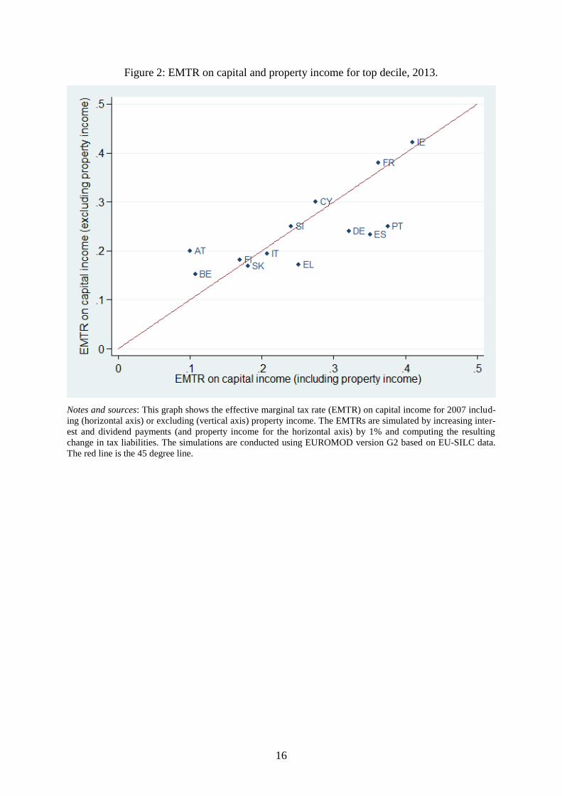
Besides interest payments and dividends, income from immovable property represents an im-

portant component of overall capital income. Its tax treatment, however, is usually different.

Firstly, dual income tax systems often tax property income at higher and progressive rates,

like labour income. The effective marginal tax rates for the top income decile are given in

Figure 2. In most countries, the EMTRs are similar to those of capital income while in some

they are lower. The reasons for this are large exemptions and deduction possibilities for prop-

erty income. For instance in Germany, the sum of taxable property income is negative in most

years.

[Figure 2 about here]

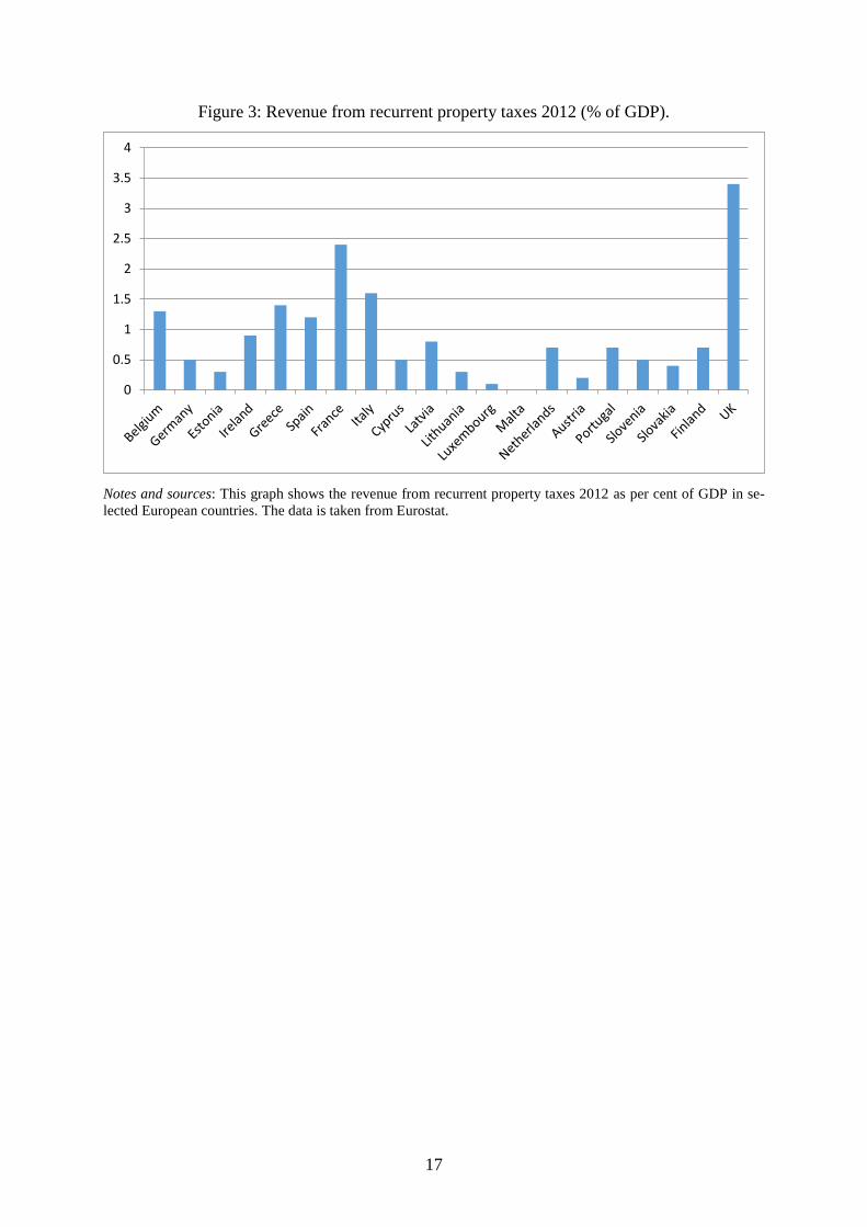
Secondly, immovable property is taxed not just through income taxation but also through tax-

es on property transactions and recurrent taxes on immovable property. Taxes on immovable

property seem attractive as a redistributive instrument because land is immobile and its supply

is fixed.

Should capital income taxation be increased to achieve more income redistribution? For in-

stance, would it be desirable to abolish dual income taxation and tax capital income at pro-

gressive rates, like labour income? For a long time the enforcement of residence-based taxes

on capital income was undermined by tax evasion through bank accounts held abroad. This

was an important reason to reduce tax rates on capital income. But recent developments in

international information exchange for tax purposes, in particular supported by the OECD and

the US government, have made it significantly more difficult for taxpayers to evade these

taxes.

However, very wealthy individuals are typically also internationally mobile in the choice of

their country of residence. This implies that higher residence based capital taxes on savings

may be effective as an instrument to redistribute income from the relatively well off to the

less well off, but the very wealthy are likely to be able to avoid these taxes.

3.2 Tax policy and growth

If it is true that higher rates of economic growth, for given rates of return on capital, have an

equalizing effect, tax reforms towards more growth friendly tax structures could have a desir-

able impact on the income distribution as well. To some extent this perspective would chal-

10

lenge the traditional view, according to which tax policy faces a fundamental trade-off be-

tween efficiency and equity.

How can the tax system be changed to achieve more economic growth? In the literature on the

link between tax structures and economic growth, the view is widespread that capital income

taxes, in particular corporate income taxes, are harmful for growth. For instance, a widely

recognized study about the impact of tax structures on economic growth conducted by the

OECD (Johansson et al., 2008) concludes:

‘The reviewed evidence and the empirical work suggests a “tax and growth ranking”

with recurrent taxes on immovable property being the least distortive tax instrument in

terms of reducing long-run GDP per capita, followed by consumption taxes (and other

property taxes), personal income taxes and corporate income taxes.’

The interpretation of the results in Johansson et al. (2008) and the empirical approach used in

this study are the subject of an ongoing and controversial debate (see Xing, 2012). Of course,

the suggestion to reduce corporate income taxes and increase consumption taxes does seem to

face the traditional efficiency equity trade-off. But this might be different for other tax in-

struments, in particular for a shift towards higher recurrent taxes on immovable property. Fig-

ure 3 gives an overview over the contribution of recurrent taxes on immovable property in

selected European countries.

[Figure 3 about here]

Figure 3 shows that the role of these taxes differs considerably, ranging from 3.4 per cent of

GDP in the United Kingdom to zero in Malta.7

This suggests that there may be room for rais-

ing more revenue from this source. Using the additional revenue to reduce labour taxes, for

instance, would probably stimulate growth and have positive effects on the income distribu-

tion.

7 One should bear in mind, though, that fees charged for local government services, which are not classified as

taxes, play a role similar to that of recurrent property taxes in some countries.

11

4. Conclusions

The so-called 𝑟 − 𝑔 model of Piketty (2014) has received enormous attention in both academ-

ic and popular circles. In its simplest characterization, it says that when existing (“old”) capi-

tal grows faster than new capital is created out of accumulated incomes, then already relative-

ly rich capital owners will become even richer relative to the others not holding capital, and

thus inequality will increase. However, economic theory offers no unambiguous support for

the view that 𝑟 > 𝑔 leads to increasing inequality. Hence, how the difference between 𝑟 and 𝑔

is related to inequality is ultimately an empirical question. Our preliminary analysis offers

some tentative support for the 𝑟 − 𝑔 model and its proposed link between the difference be-

tween 𝑟 and 𝑔 and wealth inequality. However, given the considerable problems at hand with

measurement, data availability and statistical specification, much more effort is of course

needed before we can begin to speak about stable relationships in these outcomes. This is an

important direction for future research.

We also discussed implications for tax policy under the assumption that the 𝑟 − 𝑔 model and

its link to wealth inequality is correct. Increasing the taxation of mobile capitalis only possible

on a global scale, as suggested by Piketty (2014). Experience with policy coordination in this

area suggests that this will not be possible. It therefore seems more promising to try to in-

crease 𝑔 rather than to decrease 𝑟 through tax policy. Some evidence suggests that recurrent

taxes on immovable property and consumption taxes (and other property taxes) are the least

distortive tax instrument in terms of reducing long-run GDP per capita. Increasing these taxes

and using the additional revenue to reduce labour taxes, for instance, would probably stimu-

late growth and have positive effects on the income distribution.

12

References

Acemoglu, D. and J. A. Robinson (2015). “The Rise and Decline of General Laws of Capital-

ism”. Journal of Economic Perspectives 29(1): 3–28.

Becker, J. and C. Fuest (2010). “Taxing foreign profits with international mergers and acqui-

sitions”. International Economic Review 51(1): 171–186.

Becker, J, C. Fuest and N. Riedel (2012). “Corporate Tax Effects on the Quantity and Quality

of FDI”. European Economic Review 56(8): 1495–1511.

Johansson, Å., C. Heady, J. Arnold, B. Brys and L. Vartia (2008), “Tax and Economic

Growth”, OECD Economics Department Working Paper 28.

Jones, L. E. and M. Tertilt (2008). “An Economic History of Fertility in the United States:

1826–1960.” in: P. Rupert (ed.), Frontiers of Family Economics. Bingley, West Yorkshire:

Emerald Group Publishing Limited.

Judd, K. (1985). “Redistributive Taxation in a Simple Perfect Foresight Model”. Journal of

Public Economics 28(1): 59–83.

Kotlikoff, L. and L. Summers (1987). “Tax Incidence”, in: A. Auerbach and M. Feldstein

(eds), Handbook of Public Economics, Vol. II, Amsterdam: North-Holland.

Piketty, T. (2014). Capital in the 21st century, Cambridge, MA: Belknap.

Piketty, T. (2015). "Putting Distribution Back at the Center of Economics: Reflections on

Capital in the Twenty-First Century”. Journal of Economic Perspectives 29(1): 67–88.

Piketty, T. and E. Saez (2013). “A Theory of Optimal Inheritance Taxation”. Econometrica

81(5): 1851–1886.

Piketty, T. and G. Zucman (2014), “Capital is Back: Wealth-Income Ratios in Rich Countries,

1700-2010”. Quarterly Journal of Economics 129(3): 1255–1310.

Piketty, T. and G. Zucman (2015). “Wealth and inheritance in the long run”, in: A.B. Atkin-

son and F. Bourguignon (eds.), Handbook of Income Distribution, vol.2B, Amsterdam:

North-Holland.

Roine, J., J. Vlachos and D. Waldenström (2009). “The Long-Run Determinants of Inequali-

ty: What Can We Learn from Top Income Shares?”. Journal of Public Economics 93(7–8):

974–988.

Roine, J. and D. Waldenström (2015). “Long-run trends in the distribution of income and

wealth”, In: Atkinson, A.B., Bourguignon, F. (Eds.), Handbook of Income Distribution,

vol. 2A, Amsterdam : North-Holland.

Saez, E. and G. Zucman (2014). “Wealth Inequality in the United States since 1913: Evidence

from Capitalized Income Tax Data”. NBER working paper 20625.

Xing, J. (2012). “Tax structure and growth: How robust is the empirical evidence?”. Econom-

ics Letters 117(1): 379–382.

13

Table 1: The 𝑟 − 𝑔 model and wealth inequality: Basic regressions

∆𝑇𝑜𝑝𝑊 1%𝑡 ∆𝑇𝑜𝑝𝑊 10– 1%𝑡 ∆𝐵𝑜𝑡𝑡𝑜𝑚𝑊 90%𝑡

(1) (2) (3) (4) (5) (6) (7) (8) (9)

Proxies of 𝑟:

∆𝐹𝑖𝑛. 𝑑𝑒𝑣𝑡 3.49*** 4.91*** 11.34*** 10.32*** –14.55*** –17.04***

(0.60) (1.37) (1.83) (1.47) (2.21) (2.01)

∆𝐹𝑖𝑛. 𝑑𝑒𝑣𝑡−1 1.12** 1.00 –2.61

(0.53) (1.57) (1.97)

∆𝐹𝑖𝑛. 𝑑𝑒𝑣𝑡−2 4.01*** 0.83 –4.79**

(0.60) (1.79) (2.17)

∆�̃�𝑡 2.82** 1.31 –4.57***

(1.16) (1.30) (1.71)

Proxies of 𝑔:

∆𝑌𝑡 –6.51** 0.75 –10.84* –6.27* –54.95*** –39.71*** 4.71 55.20*** 46.43***

(3.27) (3.98) (6.39) (3.70) (12.12) (8.35) (4.10) (14.78) (12.17)

∆𝑌𝑡−1 –6.19 –1.03 13.28

(4.52) (12.42) (14.88)

∆𝑌𝑡−2 10.87*** –22.87* 3.60

(3.38) (12.69) (14.30)

∆𝑔𝑡 –5.35 7.30 –3.25

(3.75) (5.73) (7.62)

Obs. 86 50 50 66 40 40 66 40 40

# countries 9 8 8 7 6 6 7 6 6

Notes and sources: ∆ denotes that variables are in first-differences. Dependent variables are shares of total per-

sonal wealth held by the top percentile (𝑇𝑜𝑝𝑊1%), top decile minus top percentile (𝑇𝑜𝑝𝑊10 − 1%) and bottom

nine deciles (𝑇𝑜𝑝𝑊1%) in the wealth distribution. 𝐹𝑖𝑛. 𝑑𝑒𝑣. denotes financial development, measured as the

sum of bank deposits and market capitalization as share of GDP, �̃� denotes proxy for rate of return to capital,

measured as the difference in first-differenced levels of financial development, 𝑌 denotes GDP per capita and 𝑔

denotes economic growth which the difference in first-differenced GDP per capita. See text for further details

and sources. All codes and data used are available on the author webpages and upon request. Robust standard

errors stand in parentheses. ***, ** and * denotes statistical significance at the 1%, 5% and 10% levels, respec-

tively.

14

Table 2: The 𝑟 − 𝑔 model and wealth inequality: Controlling for policy and institutions.

∆𝑇𝑜𝑝𝑊 1%𝑡 ∆𝑇𝑜𝑝𝑊 10– 1%𝑡 ∆𝐵𝑜𝑡𝑡𝑜𝑚𝑊 90%𝑡

(1) (2) (3) (4) (5) (6) (7) (8)

Proxies of 𝑟:

∆𝐹𝑖𝑛. 𝑑𝑒𝑣𝑡 4.42*** 7.14*** 2.05** 9.29*** 7.50*** –14.86*** –13.41***

(1.39) (1.20) (0.87) (1.43) (1.70) (1.67) (1.97)

∆𝐹𝑖𝑛. 𝑑𝑒𝑣𝑡−1 4.69***

(0.96)

∆�̃�𝑡 2.48** 4.70*** 0.90 –0.97 –4.15*** –2.37

(1.17) (1.05) (1.18) (1.39) (1.41) (1.62)

∆𝐹𝑖𝑛. 𝑑𝑒𝑣2𝑡 3.95***

(1.19)

∆�̃�2𝑡 2.10**

(0.96)

Proxies of 𝑔:

∆𝑌𝑡 –8.69 –36.08*** –17.98*** –23.62** –41.50*** –21.52* 56.23*** 61.80***

(5.65) (8.57) (6.68) (9.69) (7.41) (11.37) (9.32) (13.37)

∆𝑌𝑡−1 –19.18***

(4.22)

∆𝑌𝑡−2 15.51***

(5.90)

∆𝑔𝑡 –9.34** –15.47*** –14.25*** 1.60 2.45 11.82* 15.40**

(3.74) (3.98) (4.71) (6.25) (6.34) (6.82) (6.95)

Controls:

∆𝑃𝑜𝑝𝑡 73.60*** 76.42*** 72.91*** 61.32* 39.68 109.86** –182.26*** –152.10**

(26.42) (29.04) (28.06) (34.40) (47.59) (51.43) (55.14) (59.79)

∆𝑂𝑝𝑒𝑛𝑛𝑒𝑠𝑠𝑡 –1,470.1** –1,377.4 –2,009.9** –1,203.7 –1,150.2 1,544.4 2,597.6

(730.2) (947.0) (902.9) (1,042.7) (1,333.2) (1,256.9) (1,672.6)

∆𝐺𝑜𝑣. 𝑆𝑝𝑒𝑛𝑑𝑡 –0.23 13.09 –4.79 –0.96 –62.18*** –82.57*** 69.60*** 90.61***

(13.67) (14.35) (16.68) (16.45) (18.40) (20.62) (20.18) (26.35)

∆𝑀𝑎𝑟𝑔. 𝑡𝑎𝑥𝑡 –8.49*** –8.94*** –6.55** 5.26 6.47*

(2.17) (2.05) (2.61) (3.38) (3.66)

∆𝑇𝑜𝑝𝑌 1%𝑡 0.78*** 0.86*** 0.36 –1.44*** –1.06

(0.29) (0.28) (0.36) (0.49) (0.84)

∆𝑇𝑜𝑝𝑌10– 1%𝑡 0.08

(0.30)

∆𝐵𝑜𝑡𝑌 90%𝑡 –0.70*

(0.38)

Obs. 50 43 43 43 40 38 40 38

# countries 8 7 7 7 6 6 6 6

Notes and sources: See Table 1 for denotations of 𝐹𝑖𝑛. 𝐷𝑒𝑣., �̃�, 𝑌 and 𝑔. Dependent variables are shares of total

personal wealth held by the top percentile (𝑇𝑜𝑝𝑊1%), top decile minus top percentile (𝑇𝑜𝑝𝑊10 − 1%) and

bottom nine deciles (𝑇𝑜𝑝𝑊1%) in the wealth distribution. 𝑃𝑜𝑝. denotes population, 𝑂𝑝𝑒𝑛𝑛𝑒𝑠𝑠 the trade share in

GDP, 𝐺𝑜𝑣. 𝑆𝑝𝑒𝑛𝑑. is central government expenditures over GDP, 𝑀𝑎𝑟𝑔. 𝑡𝑎𝑥 is top marginal income tax rate,

and 𝑇𝑜𝑝𝑌1%, 𝑇𝑜𝑝𝑌10 − 1% and 𝐵𝑜𝑡𝑌90% are income shares of the top percentile, top decile minus top per-

centile and bottom nine deciles, respectively. See text for further details and sources. All codes and data used are

available on the author webpages and upon request. Robust standard errors stand in parentheses. ***, ** and *

denotes statistical significance at the 1%, 5% and 10% levels, respectively.

15

Figure 1: EMTR on capital income for top decile, difference between 2007 and 2013.

Notes and sources: This graph shows the effective marginal tax rate (EMTR) on capital income for 2007 (hori-

zontal axis) and 2013 (vertical axis). The EMTRs are simulated by increasing interest and dividend payments by

1% and computing the resulting change in tax liabilities. The simulations are conducted using EUROMOD ver-

sion G2 based on EU-SILC data. The red line is the 45 degree line.

16

Figure 2: EMTR on capital and property income for top decile, 2013.

Notes and sources: This graph shows the effective marginal tax rate (EMTR) on capital income for 2007 includ-

ing (horizontal axis) or excluding (vertical axis) property income. The EMTRs are simulated by increasing inter-

est and dividend payments (and property income for the horizontal axis) by 1% and computing the resulting

change in tax liabilities. The simulations are conducted using EUROMOD version G2 based on EU-SILC data.

The red line is the 45 degree line.

17

Figure 3: Revenue from recurrent property taxes 2012 (% of GDP).

Notes and sources: This graph shows the revenue from recurrent property taxes 2012 as per cent of GDP in se-

lected European countries. The data is taken from Eurostat.

0

0.5

1

1.5

2

2.5

3

3.5

4