by

http://ssrn.com/abstract_id=322224

Thomas A. Lubik and Frank Schorfheide

“Testing for Indeterminacy:

An Application to U. S. Monetary Policy”

PIER Working Paper 02-025

Penn Institute for Economic Research Department of Economics University of Pennsylvania

3718 Locust Walk Philadelphia, PA 19104-6297

pier@econ.upenn.edu http://www.econ.upenn.edu/pier

Testing for Indeterminacy:

An Application to U.S. Monetary Policy∗

Thomas A. Lubik

Department of Economics

Johns Hopkins University†

Frank Schorfheide

Department of Economics

University of Pennsylvania‡

July, 2002

JEL CLASSIFICATION: C11, C52, C62, E52

KEY WORDS: Econometric Evaluation and Testing, Rational

Expectations Models, Indeterminacy, Monetary

DSGE Models

∗We would like to thank Jinill Kim, Peter Ireland, and seminar participants at Johns Hopkins

University, the University of Pennsylvania, Tilburg University, the NBER Summer Institute, the

North American Econometric Society Summer Meeting in Los Angeles, the Meetings of the Society

for Computational Economics in Aix-en-Provence for insightful comments and suggestions. The

second author gratefully acknowledges financial support from the University Research Foundation

of the University of Pennsylvania.†Mergenthaler Hall, 3400 N. Charles Street, Baltimore, MD 21218. Tel.: (410) 516-5564. Fax:

(410) 516-7600. Email: thomas.lubik@jhu.edu‡McNeil Building, 3718 Locust Walk, Philadelphia, PA 19104. Tel.: (215) 898-8486. Fax: (215)

573-2057. Email: schorf@ssc.upenn.edu

Testing for Indeterminacy:

An Application to U.S. Monetary Policy

Abstract

This paper considers a prototypical monetary business cycle model for the

U.S. economy, in which the equilibrium is undetermined if monetary policy

is ‘inactive’. In previous multivariate studies it has been common practice

to restrict parameter estimates to values for which the equilibrium is unique.

We show how the likelihood-based estimation of dynamic stochastic general

equilibrium models can be extended to allow for indeterminacies and sunspot

fluctuations. We propose a posterior odds test for the hypothesis that the

data are best explained by parameters that imply determinacy. Our empiri-

cal results show that the Volcker-Greenspan policy regime is consistent with

determinacy, whereas the pre-Volcker regime is not. We find that before 1979

non-fundamental sunspot shocks may have contributed significantly to inflation

and interest rate volatility, but essentially did not affect output fluctuations.

1

1 Introduction

Economists are increasingly making use of dynamic stochastic general equilibrium

(DSGE) models for macroeconomic analysis. In order to solve these models and

keep them tractable, linear rational expectations (LRE) models are typically used

as local approximations. However, it is well known that LRE models can have

multiple equilibria. This implies that for every sequence of exogenous shocks there

exists more than one sequence of rational expectations errors for which the model

dynamics are stable. Under equilibrium indeterminacy non-fundamental sunspot

shocks can influence equilibrium allocations and induce business cycle movements

that would not be present under determinacy.

Indeterminacy often arises in business cycle models where a monetary author-

ity follows an interest rate rule. For instance, if the nominal interest rate is not

raised aggressively enough in response to an increase in inflation, the local equi-

librium dynamics are indeterminate. Hence, a central bank that wants to stabilize

aggregate fluctuations should avoid policies that lead to this possibility. It has been

suggested by Clarida, Galı, and Gertler [5] that the Federal Reserve’s policy rule

before 1979 was inconsistent with equilibrium determinacy. Beginning with Paul

Volcker’s tenure as Board Chairman and, later on, Alan Greenspan’s the Federal

Reserve implemented a much more aggressive rule that suppresses self-fulfilling ex-

pectations. Studying indeterminacy can therefore contribute to our understanding

of the macroeconomic instability during the 1970s and further the design of benefi-

cial policy rules.

The main objective of this paper is to develop an econometric framework for as-

sessing the quantitative importance of indeterminacy. We use a Bayesian approach

to evaluate the indeterminacy hypothesis by the posterior probability of the param-

eter region for which multiple stable equilibria exist. While in DSGE models with

indeterminacies not all parameters are identifiable, we show that the structure of the

models nevertheless generates testable implications for the endogenous dynamics.

By introducing sunspot shocks we essentially characterize the set of multiple equi-

2

libria. Our approach enables us to estimate the stochastic properties of the sunspot

shocks and to evaluate its contribution to the fluctuation of, for instance, output,

inflation, and interest rates.

We apply our procedure to a New Keynesian business cycle model and revisit

the question whether U.S. monetary policy was stabilizing pre- and post-Volcker.

Our estimates confirm earlier univariate studies that U.S. monetary policy before

1979 has contributed to aggregate instability and that policy has become markedly

more stabilizing during the Volcker-Greenspan period. Based on our variance de-

compositions, sunspot shocks increased the variability of inflation significantly prior

to 1979, but essentially did not affect the volatility of output.

Previous empirical studies of indeterminacy fall broadly into two categories:

First, calibration exercises, such as Farmer and Guo [7], Perli [24], Schmitt-Grohe

[32, 33], or Thomas [37], that attempt to quantify the extent to which sunspot

shocks are helpful in matching model properties to business cycle facts. They face

the common difficulty of specifying the stochastic properties of the sunspot shock.

The typical practice is to choose its variance to match the observed variance of out-

put. While these authors demonstrate the qualitative importance of indeterminacy,

their quantitative conclusions are more tenuous. As we show in this paper, equi-

librium indeterminacy does not imply that aggregate fluctuations are in fact driven

by sunspots. An alternative empirical approach is taken by Farmer and Guo [8],

Salyer [29] and Salyer and Sheffrin [30]. They try to identify sunspot shocks from

rational expectations residuals that are left unexplained by exogenous fundamentals.

Although this approach imposes more structure than simple calibration, it cannot

distinguish between omitted fundamentals and actual sunspots.

The closest theoretical and empirical precursors1 to this paper are Kim [19], Ire-

land [16], and Rabanal and Rubio-Ramirez [27] who estimate monetary models sim-

ilar to ours with likelihood-based techniques. Ireland [16] finds significant evidence1In a much earlier contribution Jovanovic [17] provides a general characterization of the identi-

fication problems inherent in econometric analyses of models with multiple equilibria. Cooper [6]

surveys different empirical approaches to indeterminacy from several fields.

3

of a change in monetary policy behavior after 1979. However, all of the above au-

thors explicitly rule out indeterminate equilibria in their estimation strategy. Since

the parameters of the monetary policy rule potentially imply indeterminacy, this

approach may result in model misspecification and biased parameter estimates.

Our paper also builds on ideas in Clarida et al. [5], who estimate a univariate

monetary policy rule by GMM over the two subsamples and argue that the pre-

Volcker estimates imply indeterminacy. However, univariate estimation results tend

to be fragile with respect to the choice of instruments. The potential presence of

sunspot fluctuations may cause identification problems that are not readily transpar-

ent in a univariate analysis. We provide an example in which the policy parameter

is only identifiable under indeterminacy. Indeterminacy is a property of a dynamic

system and should therefore be studied through a multivariate analysis. Moreover,

the boundary of the determinacy region is generally a function of both the policy

parameters and the structural parameters of the model. An accurate assessment

requires therefore the joint estimation of all parameters.

This paper is structured as follows. In the next section, we present a structural,

New Keynesian monetary business cycle model where the possibility of indetermi-

nacy arises due to the specification of the monetary policy rule. The log-linearized

business cycle model belongs to the class of LRE models. In Section 3 we derive

and compare the autocovariance properties of LRE models under both determinacy

and indeterminacy. Section 4 develops a posterior odds test for indeterminacy. A

simplified version of the monetary model is solved analytically in Section 5 in order

to illustrate the test procedure. Empirical results for the full model are presented in

Section 6. Section 7 concludes and the Appendix contains proofs and computational

details.

2 A Model for the Analysis of Monetary Policy

We study a monetary business cycle model with optimizing households and monop-

olistically competitive firms that face nominal price adjustment costs. The central

4

bank follows a monetary policy rule that adjusts the nominal interest rate in re-

sponse to changes in the target variables. The model is a variant of what is often

referred to as the New Keynesian IS-LM model. Related descriptions and deriva-

tions can be found, among others, in Galı and Gertler [11], King [20], King and

Wolman [21], and Woodford [38].

2.1 The Household

The economy is populated by a representative household that derives utility from

consumption c and real balances M/P , and disutility from working, where n denotes

the labor supply:

Ut = Et

∞∑s=t

βs−t

c

1− 1τ

s − 11− 1

τ

+ χ logMs

Ps− ns

. (1)

0 < β < 1 is the discount factor, τ > 0 the intertemporal substitution elasticity,

and χ > 0 is a scale factor. P is the economy-wide nominal price level which the

household takes as given. We define the (gross) inflation rate πt = Pt/Pt−1.

The household supplies perfectly elastic labor services to the firms period by

period for which it receives the real wage w. The household has access to a domestic

capital market where nominal government bonds B are traded that pay (gross)

interest R. Furthermore, it receives aggregate residual profits Π from the firms and

has to pay lump-sum taxes T . Consequently, the household maximizes (1) subject

to its budget constraint:

ct +Bt

Pt+

Mt

Pt+

Tt

Pt= wtnt +

Mt−1

Pt+ Rt−1

Bt−1

Pt+ Πt. (2)

The usual transversality condition on asset accumulation applies which rules out

Ponzi-schemes. Initial conditions are given by B0. The household’s behavior is

described by the following first-order conditions:

c−1/τt = IEt

[β

Rt

πt+1c−1/τt+1

], (3)

Mt

Pt= χ

Rt

Rt − 1c1/τt , (4)

wt = c1/τt . (5)

5

and the budget constraint (2).

Equation (3) is the usual consumption Euler equation. Expected consumption

growth is thus an increasing function of the real interest rate, which is defined as

the nominal interest rate adjusted for (expected) inflation. A monetary policy that

controls the nominal interest rate thus affects the time path of consumption. It

is through this channel that the possibility of indeterminacy arises. Equation (4)

is a standard, interest-sensitive money-demand schedule. Once consumption and

the nominal rate are determined, real balances adjust automatically in equilibrium.

Specification of an interest rate rule is therefore enough to close the model, and the

money demand equation plays no additional role in deriving a solution. Finally, (5)

is the utility-weighted labor-supply equation.

2.2 The Firms

The production sector is described by a continuum of monopolistically competitive

firms each of which faces a downward-sloping demand curve for its differentiated

product:

pt(j) =(

yt(j)yt

)−1/ν

Pt. (6)

This demand function can be derived in the usual way from Dixit-Stiglitz prefer-

ences, whereby pt(j) is the profit-maximizing price consistent with production level

yt(j). The parameter ν is the elasticity of substitution between two differentiated

goods. As ν → ∞ the demand function becomes perfectly elastic and the differen-

tiated goods become substitutes. The aggregate price level and aggregate demand

yt are beyond the control of the individual firm.

We introduce nominal rigidity by assuming that firms are subject to quadratic

adjustment costs in nominal prices. When a firm wants to change its price beyond

the general trend in prices, given by the economy-wide inflation rate π, it incurs

‘menu costs’ in the form of lost output. The parameter ϕ ≥ 0 governs the degree of

stickiness in the economy. Production is assumed to be linear in labor nt(j), which

6

each firm hires from the household:

yt(j) = Atnt(j). (7)

Total factor productivity At is an exogenous process. Note that At affects all firms

in the same way.

The firm j thus chooses factor input nt(j) to maximize:

IEt

[ ∞∑s=t

qsΠs(j)

]= IEt

[ ∞∑s=t

qs

[ps(j)Ps

ys(j)− wsns(j)− ϕ

2

(ps(j)

ps−1(j)− π

)2

ys

]]

(8)

subject to (6) and (7). q is the (potentially) time-dependent discount factor that

firms use to evaluate future profit streams. Under the assumption of perfect in-

surance markets qt+1

qt= β

(ct

ct+1

)1/τ. In other words, since the household is the

recipient of the firms’ residual payments it directs firms to make decisions based on

the households intertemporal rate of substitution (see Kim [19]).

Although firms are heterogeneous ex ante, we impose the usual solution concept

for this kind of production structure: We assume that firms behave in an identical

way so that the individual firms can be aggregated into a single representative,

monopolistically competitive firm. The firm’s first-order conditions after imposing

the homogeneity assumption are:

nt =yt

wt

(1− 1

ϑt

), (9)

1ϑt

=1ν

IEt

[1− ϕ (πt − π) πt + β

(ct

ct+1

)1/τ

ϕ (πt+1 − π) πt+1yt+1

yt

]. (10)

ϑt can be interpreted as the output demand elasticity augmented by the cost of

price adjustment. Note that the mark-up of price over marginal cost is(1− 1

ϑt

)−1.

In steady state, the mark-up is νν−1 , so that ν indexes the degree of monopolistic

distortion in the economy. In the perfectly competitive case, with ν →∞, the mark-

up is unity. Furthermore, when prices are perfectly flexible (ϕ = 0), or when the

monetary authority perfectly stabilizes the price level (πt = π for all t) the mark-up

is constant.

7

2.3 Monetary Policy Rules

In order to close the model we need to specify the behavior of the monetary authority.

We assume that the central bank follows a nominal interest rate rule by adjusting its

instrument in response to deviations of output and inflation from their respective

target levels. The monetary authority is also concerned about a smooth interest

rate path. We consider a monetary policy rule of the form

Rt = RρRt−1R

1−ρR∗,t eεR,t , (11)

where the target rate R∗,t evolves according to

R∗,tR

=(πt

π

)ψ1(

yt

y∗,t

)ψ2

. (12)

The shock εR,t can be interpreted as monetary policy implementation error or the

unsystematic component of monetary policy. Potential output y∗,t is defined as the

level of output that would prevail under the absence of price stickiness (ϕ = 0).

Finally, we need to specify the behavior of the fiscal authority. It is assumed

that the government levies a lump-sum tax (or subsidy) TtPt

to finance any shortfall

in government revenues (or to rebate any surplus):

Tt

Pt− Mt −Mt−1

Pt+

Bt −Rt−1Bt−1

Pt= g∗t . (13)

The fiscal authority follows a ‘passive’ rule by endogenously adjusting the primary

surplus to changes in the government’s outstanding liabilities. The monetary au-

thority, on the other hand, is free to pursue an active or a passive policy. g∗t denotes

aggregate government purchases. We assume for simplicity that the government con-

sumes a fraction of each individual good: g∗t (j) = ζtyt(j).2 Define γt = 1/(1 − ζt).

The aggregate demand can then be written in log-linear form as: ln yt = ln ct +ln γt.

2.4 Equilibrium and Log-linear Approximation

In order to find a solution to the model, we log-linearize the equations describing

the equilibrium around a deterministic steady state. The log-linearized equation2See Galı [10] for a derivation and justification of this assumption.

8

system can be reduced to three equations in output yt, inflation πt and the nominal

interest rate Rt, where xt = ln xt − lnx:

yt = IEt[yt+1]− τ(Rt − IEt[πt+1]) + γt − IEt[γt+1], (14)

πt = βIEt[πt+1] +ν − 1τϕπ2

[yt − (τAt + γt)], (15)

Rt = ρRt−1 + (1− ρ)(ψ1πt + ψ2[yt − (τAt + γt)]

)+ εR,t, (16)

The potential output y∗,t = τAt+γt. The overall degree of distortion in the economy

is measured by κ = (ν−1)/(τϕπ2). Eq. (14), often referred to as the New Keynesian

IS-curve, is an intertemporal Euler-equation, while (15) is derived from firms’ opti-

mal price-setting problem and governs inflation dynamics around the steady state

π ≥ 1. This relation can be interpreted as an (expectational) Phillips-curve with

slope κ. Eq. (16) is the log-linearized monetary policy rule where 0 ≤ ρ < 1 is

the smoothing coefficient and ψ1, ψ2 ≥ 0 are the policy parameters. We define the

exogenous processes3

gt = γt − IEt[γt+1] (17)

zt = τAt + γt (18)

and assume that both gt and zt evolve according to univariate AR(1) processes with

autoregressive coefficients ρg and ρz, respectively. The innovations of the AR(1)

processes are denoted by εg,t and εz,t and assumed to be correlated.

3 Autocovariance Properties of Linear Rational Expec-

tations Models

The log-linearized DSGE model presented in the previous section can be written as

a linear rational expectations (LRE) model of the form

Γ0(θ(1))st = Γ1(θ(1))st−1 + Ψ(θ(1)) + Π(θ(1))ηt, (19)

3Instead of imposing the cross-equation restrictions derived from the theoretical model we allow

for a more general covariance structure. This follows common practice in the related literature (see,

for instance, Galı [10]). We will return to this issue in Section 5.3.

9

where

st = [yt, πt, Rt, IEt[yt+1], IEt[πt+1], gt, zt]′

εt = [εR,t, εg,t, εz,t]′

ηt = [(yt − IEt−1[yt]), (πt − IEt−1[πt])]′

and θ(1) ∈ Θ(1) stacks the structural parameters of the DSGE model. In general, let

st be a n× 1 vector. Moreover, the dimension of the vector of fundamental shocks

εt is l×1 and the dimension of the vector of expectation errors ηt is k×1. The LRE

system has a stable solution if one can choose the expectation errors ηt to suppress

the explosive components of st.

We assume that in addition to the fundamental shocks εt agents observe a p× 1

vector of sunspot shocks ζt. These sunspot shocks can potentially influence the en-

dogenous variables through the expectation formation embodied in ηt. Fundamental

and sunspot shocks are regarded as exogenous. The expectation errors ηt are linear

functions of εt and ζt

ηt = η1(εt) + η2(ζt) (20)

with the property ηi(0) = 0 and hence considered endogenous. The solution of

the LRE system is unique (determinacy) if there is only one mapping from the

fundamental shocks to the expectation errors for which st is non-explosive and ηt

does not depend on the sunspot shocks. Indeterminacy refers to the case in which

there are many mappings from the fundamental shocks to the expectation errors

and sunspot shocks potentially affect the expectation formation. Let νt = [ε′t, ζ ′t]′.

Throughout this section we will assume that νt has mean zero and variance Σνν

conditional on the information set generated by past νt’s.

The DSGE model is used to obtain a probabilistic representation for a m × 1

vector of observable variables, related to st through the linear relationship

xt = Ξst. (21)

Under the LRE model xt is a linear function of current and past shocks νt. Since

νt has a constant variance and we restrict ourselves to stable solutions of the LRE

10

model the process xt is covariance stationary and its stochastic properties can be

characterized through its autocovariance sequence Γxx,h = IE[xtx′t−h], h = 0, 1, 2, . . ..

The goal of this paper is to devise an empirical test of determinacy versus indeter-

minacy. Hence, we will begin by showing to what extent the autocovariance pattern

of xt is distinguishable under the two regimes.

In solving the LRE system we closely follow the approach by Sims [35], extended

in Lubik and Schorfheide [23].4 To keep the exposition simple we assume that the

matrix Γ0 in Eq. (19) is invertible.5 The system can be rewritten as

st = Γ∗1st−1 + Ψ∗εt + Π∗ηt. (22)

Replace Γ∗1 by its Jordan decomposition JΛJ−1 and define the vector of transformed

model variables wt = J−1st. Let the i’th element of wt be wi,t and denote the i’th

row of J−1Π∗ and J−1Ψ∗ by [J−1Π∗]i. and [J−1Ψ∗]i., respectively. The model can

be rewritten as a collection of AR(1) processes

wi,t = λiwi,t−1 + [J−1Π∗]i.εt + [J−1Ψ∗]i.ηt. (23)

Define the set of stable AR(1) processes as

Is(θ(1)) ={

i ∈ {1, . . . n}∣∣∣∣∣∣λi(θ(1))

∣∣ < 1}

(24)

and let Ix(θ(1)) be its complement. Let ΨJx and ΠJ

x be the matrices composed of the

row vectors [J−1Ψ∗]i. and [J−1Π∗]i. that correspond to unstable eigenvalues, i.e.,

i ∈ Ix(θ(1)). To ensure stability of st the expectation errors ηt have to satisfy

ΨJxεt + ΠJ

xηt = 0 (25)4Sims [35] solution method generalizes the method proposed by Blanchard and Kahn [2]. In

particular, it does not require the researcher to separate the list of endogenous variables into ‘jump’

and ‘predetermined’ variables. It recognizes that it is the structure of the coefficient matrices

that implicitly pins down the solution. Instead of imposing ex ante which individual variables are

‘predetermined’, Sims’ algorithm determines endogenously the linear combination of variables that

has to be ‘predetermined’ for a solution to exist.5If Γ0 is singular, a generalized complex Schur decomposition (QZ) can be used to manipulate

the system, see Sims [35].

11

for all t. Three cases can be distinguished: (i) Eq. (25) has no solution, (ii) one

solution (determinacy), and (iii) multiple solutions (indeterminacy). We will focus

on (ii) and (iii) and assume that the parameter space Θ(1) is restricted to the set of

θ(1)’s for which at least one solution to Equation (25) exists. We characterize the

solution in the following proposition, which is proved in Lubik and Schorfheide [23].

Proposition 1 Let UDV ′ be the singular value decomposition of ΠJx and partition

U = [U.1, U.2], D = diag(D11, D22), V = [V.1, V.2]. The partitions U.1 and V.1

conform with the non-zero singular values D11. If there exists a solution to Eq. (25)

that expresses the forecast errors as function of the exogenous shocks νt, it is of the

form

ηt = η1(εt) + η2(ζt) (26)

= (−V.1D−111 U ′

.1ΨJx + V.2M1)εt + V.2M2ζt,

where r is the number of singular values that are equal to zero, M1 is an r×l matrix,

M2 is an r × p matrix, and the dimension of V.2 is k × r. The solution is unique if

r = 0 and V.2 is empty.

The parameter space can be partitioned into two regions. For θ(1) ∈ ΘD(1) the

LRE system has a unique stable solution, that is, r = 0. If θ(1) ∈ ΘI(1) then r > 0

and there exist multiple stable solutions. Eq. (26) shows that indeterminacy has two

effects. First, without additional assumptions the impact of the structural shocks

on the forecast errors is not determined, since θ(1) does not pin down the matrix

M1. Second, the sunspot shocks ζt can influence the model dynamics through the

expectation errors ηt (M2 6= 0).

We will introduce the parameter vector θ(2) ∈ Θ(2) to index the matrices M1 and

M2 that appear in Eq. (26). The vector θ(2) essentially indexes the multiple equilibria

that arise under indeterminacy. The structural parameter vector is extended to

θ = [θ′(1), θ′(2)]

′ ∈ Θ. We partition the domain of θ into ΘD and ΘI , which conform

with the partitions of θ(1). If θ(1) ∈ ΘD(1) then the value of θ(2) does not matter, that

is, the models [θ′(1), θ′(2)]

′ and [θ′(1), θ′(2)]

′ are observationally equivalent.

12

Under the assumption that wi,0 = 0 for i ∈ Ix(θ(1)) we obtain the following

result

wi,t =

λi(θ(i))wi,t−1 + µi(θ(1), θ(2))νt i ∈ Is(θ(1))

0 i ∈ Ix(θ(1)),(27)

where µi can be obtained by substituting (26) into Eq. (23). Thus, by construction

of the solution some of the AR(1) processes are equal to zero. Since xt is a linear

combination of the wi,t processes, its autocovariances are given by

IE[xk,txl,t−h] =∑

i∈Is

λhi

[ ∑

j∈Is

11− λiλj

Ξk,iµiΣννµ′jΞj,l

]. (28)

More generally, the autocovariance matrices of xt have a representation of the form

Γxx,h(θ) =∑

i∈Is(θ(1))

λhi (θ(1))Di(θ(1), θ(2)). (29)

The autocovariance sequence {Γxx,h(θ∗)}∞h=0 provides enough information to classify

the parameter θ∗ ∈ ΘI as belonging to the indeterminacy region if there does not

exist a θ ∈ ΘD such that {Γxx,h(θ)}∞h=0 = {Γxx,h(θ∗)}∞h=0. Let Λ(θ) be the set of non-

repeated stable eigenvalues λi(θ(1)), i ∈ Is(θ(1)). The following proposition provides

a sufficient condition for the identifiability of indeterminacy based on autocovariance

sequences. The proposition is a direct consequence of Eq. (29).

Proposition 2 Suppose θ∗ ∈ Θs, where s ∈ {D, I}. Then θ∗ can be correctly

classified based on the sequence of autocovariances if Λ(θ) 6= Λ(θ∗) for all θ ∈ Θ\Θs.

Under indeterminacy the number of stable eigenvalues is generally larger than

under determinacy. Thus, one can expect a richer autocovariance pattern that

cannot be reproduced with parameters from the determinacy region. The intuition

for our test procedure is that indeterminacy is potentially6 identifiable based on the

autocovariance sequence of xt, which can be estimated from the data.

Since every xi,t is a linear combination of at most n AR(1) processes, the au-

tocovariance structure of xt can be reproduced with an ARMA(p,q) process, where6Two notable exceptions are indeterminacy parameters that lead to repeated eigenvalues, and

equilibria under indeterminacy for which µi(θ(1), θ(2))νt = 0 for all t and some i ∈ Is(θ(1)).

13

p ≤ n and q ≤ n− 1. We can represent

xt = At + A1xt−1 + . . . + Anxt−n + ut + B1ut−1 + . . . + Bn−1ut−n+1, (30)

where the innovations ut are functions of the fundamental shocks εt and the sunspot

shocks ζt with conditional covariance Σuu. We express Σuu and the VARMA coeffi-

cient matrices as functions of a non-redundant parameter vector φ ∈ Φ. The DSGE

model imposes nonlinear restrictions on the parameters of the VARMA representa-

tion.

4 Econometric Approach

This section develops a test of the hypothesis θ ∈ ΘD versus θ ∈ ΘI and outlines

our strategy to obtain an estimate of θ based on a sequence of endogenous variables

XT = {x1, . . . , xT }. For the remainder of the paper we assume that θ completely

characterizes the probability distribution of the observables XT so that we have

a parametric likelihood function available. This can be achieved, for instance, by

assuming that νt is normally distributed. We showed in the previous section that

testing for determinacy is closely related to determining the number of latent (non-

zero) autoregressive state variables wi,t that determine the evolution of xt.

In the context of classical hypothesis testing, determining the number of latent

state variables is a non-standard problem. Suppose under the null hypothesis, H0,

xt is driven by two latent AR(1) processes, whereas under the alternative, Ha, xt is a

function of three latent AR(1) processes. The autoregressive coefficient of the third

state process is not identifiable under the null hypothesis because the innovation to

the third state process is zero under H0. The econometric implications of param-

eters that are not identifiable under the null hypothesis have been studied from a

frequentist perspective in, for instance, Andrews and Ploberger [1] and Hansen [14].

In the case of testing determinacy versus indeterminacy the number of latent

states is only one piece of information that can be used to discriminate the two hy-

potheses. The second piece of information is embodied in the cross-equation restric-

tions that the DSGE model potentially imposes on the state space representation of

14

xt. We will use a Bayesian approach that exploits both pieces of information simul-

taneously. From a joint probability distribution of the data XT and the structural

parameters θ a posterior distribution of θ given XT will be derived. Our assessment

of the empirical relevance of indeterminacy and sunspot fluctuations is based on the

prior and posterior probability mass assigned to the indeterminacy region ΘI .

The parameter φ ∈ Φ of the reduced form VARMA representation (30) is used to

index the probability distribution of the data. The likelihood function of φ is denoted

by L(φ|XT ). The solution algorithm described in Section 3 provides a mapping Tfrom the (extended) structural parameter space Θ into the reduced form parameter

space, denoted by Φ. The mapping T , however, is not one-to-one, which creates

the identification problems in this model. For instance, if θ ∈ ΘD, the parameters

that are used to index multiple equilibria under indeterminacy, θ(2), have no effect

on the reduced form of xt. The likelihood function for the structural parameters is

given by L(T (θ)|XT ).

We will use P and PX,T to denote the prior and posterior distribution of θ.

Moreover, Q and QX,T signify prior and posterior distribution of φ. According

to Bayes Theorem, the posterior distribution of the structural parameters has the

following density (with respect to its prior distribution)

dPX,T

dP=

L(T (θ)|XT )∫L(T (θ)|XT )dP

. (31)

Since the mapping T is not one-to-one, the likelihood function is flat in some direc-

tions of the parameter space. More precisely, the likelihood function is constant on

the sets {θ : T (θ) = φ}.

The denominator in Equation (31) can be rewritten as∫

L(T (θ)|XT )dP =∫

[∫

L(T (θ)|XT )dPφ]dQ (32)

=∫

L(φ|XT )dQ,

where Pφ is the conditional prior distribution of θ given that T (θ) = φ. The distri-

bution of T (θ) under the Bayesian posterior IPX,T is the posterior distribution of

15

the reduced form parameters, denoted by QX,T . It has density

dQX,T

dQ=

L(φ|XT )∫L(φ|XT )dQ

(33)

with respect to Q.

The posterior expectation of a function f(θ) is computed as follows. First,

integrate f(θ) on the sets {θ : T (θ) = φ} with respect to the conditional prior

distribution of θ given φ, Pφ. The likelihood function is constant on these sets and

the data do not lead to an updating of the distribution Pφ.7 Second, the reduced

form parameter φ is integrated out with respect to its posterior, QX,T . Since the

likelihood function is informative about φ its distribution is updated. Formally,∫

f(θ)dPX,T =∫

f(θ)L(T (θ)|XT )∫L(T (θ)|XT )dP

dP (34)

=∫ [∫

f(θ)L(T (θ)|XT )∫L(T (θ)|XT )dP

dPφ

]dQ

=∫ [∫

f(θ)dPφ

]dQX,T .

Despite a lack of identification of the structural parameters, the prior distribution

of θ is updated in the directions in which the data are informative and the resulting

posterior distribution can be used for inference.

The probability mass assigned to the indeterminacy region of the structural

parameter space will be used to assess the evidence in favor of the indeterminacy

hypothesis. The prior probability mass is given by

π0(I) =∫ [∫

{θ ∈ ΘI}dPφ

]dQ, (35)

whereas the posterior probability mass is

πT (I) =∫ [∫

{θ ∈ ΘI}dPφ

]dQX,T . (36)

Suppose that data are generated from the LRE model (19, 21) with parameters

θ0. Let φ0 = T (θ0). Under mild regularity conditions, e.g. Kim [18], the posterior7This is a general feature of Bayesian inference for models with non-identifiable parameters, see

Poirier [26].

16

distribution of the reduced form parameters begins to concentrate around φ0 as

more observations become available. The posterior probability of indeterminacy

will asymptotically converge to the prior probability of indeterminacy conditional

on the reduced form parameters taking the ‘true’ value φ0. The result is summarized

in the following proposition. ‘p−→’ signifies convergence in distribution under the

probability distribution of XT .

Proposition 3 Let a δ-neighborhood of φ0, Nδ(φ0), be a subset of Φ such that

|φ − φ0| < δ. Suppose there exists a collection of δ-neighborhoods {Nδ(φ0)}δ>0

such that g(φ) =∫ {θ ∈ ΘI}dPφ is continuous at φ0 within Nδ(φ0) and the posterior

distribution of φ concentrates in the δ-neighborhood in the sense∫Nδ(φ0) dQX,T

p−→ 1,

then

πT (I)p−→

∫{θ ∈ ΘI}dPφ0 (37)

as T −→∞.

Suppose that data are generated from the indeterminacy region, θ0 ∈ ΘI , and

the distribution of XT under θ0 is distinguishable, e.g., based on the number of

latent AR(1) processes, from the distributions that can arise under determinacy,

that is, T −1(φ0) ∈ ΘI .8 The Proposition implies that in this case the posterior

probability of indeterminacy will tend to one. Regardless of their prior distribu-

tion, econometricians will reach the same conclusion as T −→ ∞. If the reduced

form representation is consistent with both regimes then the posterior probability

of indeterminacy will converge to the prior probability conditional on φ0. We will

examine the concentration of the posterior and the consistency of the posterior-

probability based assessment of the indeterminacy hypothesis in the specific context

of the monetary DSGE model.8The set T −1(φ) is defined as {θ ∈ Θ : T (θ) = φ}.

17

5 A Simplified Version of the Monetary DSGE Model

Before applying our solution method and inference procedure to the full model

described in Section 2, we will study a simplified version of the DSGE model ana-

lytically. We assume that the monetary authority does not attempt to smooth the

nominal interest rate (ρR = 0), and it only targets current inflation (ψ2 = 0). Fur-

thermore, the exogenous processes gt and zt are serially uncorrelated (ρg = ρz = 0).

Define the conditional expectations ξyt = IEt[yt+1], ξπ

t = IEt[πt+1], and the expecta-

tion errors ηyt = yt−ξy

t−1, ηπt = πt−ξπ

t−1. Instead of applying the solution algorithm

to the full DSGE model, we exploit its block-triangular structure. Notice that

yt

πt

Rt

=

1 0

0 1

0 ψ1

ξy

t

ξπt

+

0

0

1

εR,t +

1 0

0 1

0 ψ1

ηy

t

ηπt

. (38)

The conditional expectations ξt = [ξyt , ξπ

t ]′ evolve according to

ξt =

1 + κτ

β τ(ψ1 − 1β )

−κβ

1β

︸ ︷︷ ︸Γ∗1

ξt−1 +

τ −1 0

0 0 κ

︸ ︷︷ ︸Ψ∗

εt +

1 + κτ

β τ(ψ1 − 1β )

−κβ

1β

︸ ︷︷ ︸Π∗

ηt.

(39)

The vector of expectation errors ηt = [ηyt , ηπ

t ]′ can be determined by solving the

two-dimensional subsystem (39). Replace Γ∗1 by its Jordan decomposition JΛJ−1,

define wt = J−1ξt, and rewrite the model as

wt = Λwt−1 + J−1Ψ∗εt + J−1Π∗ηt. (40)

Tedious but straightforward algebra yields the eigenvalues that appear in the diag-

onal matrix Λ in Eq. (40):

λ1, λ2 =12

(1 +

κ + 1β

)−+

12

√(κ + 1

β− 1

)2

+4κ

β(1− ψ1). (41)

It can be shown9 that the determinacy properties of this model solely hinge on the

policy parameter ψ1.9See Bullard and Mitra [3] or Lubik and Marzo [22].

18

5.1 Determinacy

If ψ1 > 1 then both λ1 and λ2 are greater than one in absolute value. Thus,

Ix(θ(1)) = {1, 2} if θ(1) ∈ ΘD(1). The only stable solution of (39) is ξt = 0, which is

obtained if ξ0 = 0 and

ηt = −Π∗−1

Ψ∗εt = − 11 + κτψ1

τ −1 −τκψ1

κτ −κ κ

εt. (42)

Thus, the expectation errors ηt are uniquely determined as functions of the structural

shocks and the evolution of output, inflation, and interest rates is given by

yt

πt

Rt

=

11 + κτψ1

−τ 1 τκψ1

−κτ κ −κ

1 κψ1 −κψ1

εR,t

εg,t

εz,t

. (43)

The model exhibits no dynamics because the solution suppresses the two roots of the

autoregressive matrix Γ∗1. An unanticipated monetary contraction leads to a one-

period fall in output and inflation. An Euler-equation shock εg,t increases output,

inflation, and interest rate. A Phillips-curve shock εz,t raises output, but lowers

inflation and interest rates for one period.

5.2 Indeterminacy

If the inflation elasticity of the interest rate rule is less than one, then the smaller of

the two eigenvalues, λ1, is less than one and only the second element, w2,t, of the 2×1

vector wt is explosive. Thus, Ix(θ(1)) = {2} and the stability condition (25) consists

of one equation, that does not uniquely determine the 2 × 1 vector of expectation

errors ηt. The full set of solutions for ηt is given by Proposition 1.

It is useful to transform the representation of ηt given in Proposition 1 as fol-

lows. Notice that in this model the set Ix(θ(1)) = {1, 2} = IDx is constant in the

determinacy region θ(1) ∈ ΘD(1) and nests Ix(θ(1)) = {2} for θ(1) ∈ ΘI

(1). Thus, one

solution to the stability condition can be obtained by using the equations

[J−1Π∗]i.εt + [J−1Ψ∗]i.ηt (44)

19

for i ∈ IDx even though θ(1) ∈ ΘI

(1). For the simple monetary model we obtain

ηt =

− 1

1 + κτψ1

τ −1 −τκψ1

κτ −κ κ

+

(λ2 − 1− κτψ1)

κλ2

M1

εt

+

(λ2 − 1− κτψ1)

κλ2

ζ∗t , (45)

where ζ∗t = M2ζt is a normalized sunspot shock and M1 is a 1 × 3 matrix that is

not determined by the parameters θ(1) of the DSGE model. It can be shown that

both λ2 ≥ 0 and λ2− 1−κτψ ≥ 0. Thus a positive normalized sunspot shock raises

the expectation errors in output and inflation. The effect of the structural shocks

on the expectation errors is not uniquely determined.

Define the following linear combination of fundamental shock and sunspot shocks

η∗t =

(λ2 − 1− κτψ1)

κλ2

(M1εt + ζ∗t ). (46)

The law of motion for output, inflation, and interest rate becomes

yt

πt

Rt

=

11 + κτψ1

−τ 1 τκψ1 (λ2 − 1− κτψ1)

−κτ κ −κ κλ2

1 κψ1 −κψ1 ψ1κλ2

εR,t

εg,t

εz,t

η∗t

(47)

+

(β(λ2 − 1)− τκ)/κ

1

ψ1

w1,t−1,

where w1,t follows the AR(1) process

w1,t = λ1w1,t−1 + µ1η∗t . (48)

In the indeterminacy case only one root of Γ∗1 is suppressed and the endogenous

variables are generally serially correlated through the process w1,t. Notice that the

fundamental shocks εt affect the latent process w1,t only indirectly through η∗t . Thus,

if M1 = 0 the effects of fundamental shocks vanish after one period.

20

5.3 Orthogonal Shocks

The monetary DSGE model is driven by three fundamental shocks, namely a mon-

etary policy shock εR,t, a shock to the Euler equation, εg,t, a shock to the Phillips

curve, εz,t, and potentially a sunspot shock, ζ∗t . We assume that the sunspot shock

ζ∗t is unrelated to the fundamental shocks εt. Moreover, the monetary policy shock is

uncorrelated with εg,t and εz,t, as the reaction function of the central bank captures

any systematic responses of the monetary policy to changes in the fundamentals.

While we allow εg,t and εz,t to be generally correlated, we assume that they are

functions of orthogonal ‘demand’ and ‘supply’ shocks. The ‘demand’ shock, such as

a government spending shock, shifts both the Euler equation and the Phillips curve,

whereas the ‘supply’ shock, such as a technology shock, only affects the price setting

equation (see Section 2).

Let νt = [εR,t, εg,t, εz,t, η∗t ]′, where η∗t is defined in Eq. (46). To complete the

probabilistic specification of the model, let νt ∼ iidN (0,Σνν), where

Σνν =

σ2R 0 0 ρRησRση

σ2g ρgzσgσz ρgησgση

σ2z ρzησzση

σ2η

. (49)

The correlations are restricted to ensure that the covariance matrix is positive. The

correlations ρRη, ρgη, and ρzη arise because the effect of the fundamental shocks on

the expectation errors, i.e., the matrix M1 in Eq. (46), is not uniquely pinned down

under indeterminacy. In the notation of Section 3, the correlations would enter the

extension θ(2) of the structural parameter vector.

The relationship between νt and the normalized and orthogonalized shocks is

given by

εR,t

εg,t

εz,t

η∗t

=

c11 0 0 0

0 c22 c23 0

0 0 c33 0

c41 c42 c43 c44

εR,t

εg,t

εz,t

ζ∗t

. (50)

21

The coefficients cij can be uniquely determined from the covariance matrix Σνν . If

M1 = 0 in Eq. (46) then ρRη = ρgη = ρzη = 0 and c41 = c42 = c43 = 0. In this case

the orthogonalized fundamental shocks do not enter the model through η∗t and the

response of the endogenous variables to the fundamental shocks is continuous in the

parameters at the boundary of the determinacy region ψ1 = 1. If in addition the

variance of the sunspot shock ζ∗t is zero, then ση = 0 and Eq. (47) reduces to the

law of motion obtained under determinacy in Eq. (43).

5.4 Identification of Indeterminacy Regimes in Large Samples

This section examines whether the posterior probability of indeterminacy is consis-

tent in the sense that it converges to one if XT was generated from the indeterminacy

region and to zero otherwise. The (extended) vector of structural parameters of the

simplified monetary DSGE model is

θ = [ψ1, κ, τ, ρgz, ρRη, ρgη, ρzη, σR, σg, σz, ση]′ ∈ Θ ⊂ IR11. (51)

The results of Section 5.1 and 5.2 imply that the reduced form of the DSGE model

is ARMA(1,1):

xt = Axt−1 + ut + But−1, ut ∼ iidN (0,Σuu). (52)

We express the ARMA coefficient matrices A, B, and Σuu as functions of the reduced

parameter vector φ = [φ′1, φ′2]′. We assume that the reduced form parameters are

defined such that Σuu = Σuu(φ1), A = A(φ2), B = B(φ2), A(0) = 0, and B(0) =

0. Thus, φ1 indexes the covariance matrix Σuu of the reduced-form innovations

ut, whereas φ2 determines the autoregressive and moving-average structure of the

process. If φ2 = 0 then xt has no serial correlation.

The prior distribution of θ is assumed to be continuous with the property that

0 < π0(I) =∫ {ψ1 > 1}dP < 1. According to Eq. (36) the first step of the analysis

is to determine∫ {θ ∈ ΘI}dPφ:

∫{θ ∈ ΘI}dPφ =

1 if φ2 6= 0

0 if φ2 = 0. (53)

22

If φ2 6= 0 it can be deduced that T −1(φ) ∈ ΘI because only indeterminacy can gen-

erate autocorrelation. If φ = 0, that is, xt has no serial correlation, the information

is inconclusive. The covariance matrix Σuu does not uniquely determine ψ1 and the

lack of serial correlation does not only arise in the determinacy case, but also under

indeterminacy if the standard deviation of the composite shock η∗t is equal to zero.

Given the other structural parameters, our prior assigns probability zero to

{ση = 0} and probability one to {ση > 0}. Since under determinacy φ2 = 0

for arbitrary values of ση we conclude that the prior probability of indeterminacy

conditional on no serial correlation is equal to zero.10

The second step of the large sample analysis is to examine the continuity of

g(φ) =∫ {θ ∈ ΘI}dPφ and the concentration of the posterior distribution QX,T .

According to Eq. (53), g(φ) is continuous for φ2 6= 0. If φ = [φ′1, 0]′, then g(φ) is

in general discontinuous because an arbitrary small deviation from φ2 = 0 changes

g(φ) from zero to one. However, continuity is preserved within neighborhoods that

lie in the subspace of φ for which φ2 = 0. Thus, in order to apply Proposition 3 to

φ0 = [φ′1,0, 0] it has to be shown that the posterior distribution QX,T concentrates

in the subspace of Φ for which φ2 = 0. Details are provided in the Appendix. The

result is summarized in the following proposition.

Proposition 4 Suppose XT is generated according to the LRE model given in

Eq. (38) and (39) with innovations νt ∼ (0, Σνν) and the prior distribution P of

Θ is continuous then the posterior probability of the indeterminacy region converges

to

πT (I)p−→

0 if θ ∈ ΘD

1 if θ ∈ ΘI(54)

except for a subset of the parameter space that has prior probability zero.

Proposition 4 states that the Bayesian test for indeterminacy is consistent.11 It

is instructive to compare our Bayesian test to an alternative procedure that has been10Under a prior distribution that assigns non-zero mass to ση = 0 the prior probability of inde-

terminacy given φ2 = 0 could be non-zero.11The proposition could be extended to cases in which XT is generated from a more general

23

applied by Clarida et al. [5] in the context of the full model specified in Section 2.

Since the inflation elasticity of the interest rate is a perfect regime classifier, it

appears plausible to estimate ψ1 based on

Rt = ψ1πt + εR,t (55)

and compare the estimate to unity. According to the results in Section 5.1 and 5.2

the equilibrium inflation rate is a function of εR,t. Hence simple OLS estimation of

ψ1 will lead to an inconsistent estimate.

Instrumental variable (IV) estimation is also problematic. As long as the sunspot

shock ηt is zero at all times, πt is only a function of the current shocks. Since output

is correlated both with the demand shock and the monetary policy shock it is not a

valid instrument. Thus, there is no observable variable that could serve directly as

an instrument.

The only remaining possibility is to use lagged values of inflation, output, or

interest rates as instruments. However, this approach is only successful if the data

were generated under the indeterminacy regime and ση > 0. Thus, although plau-

sible at first glance, testing for indeterminacy based on a univariate estimate of the

reaction function is not feasible in the model examined in this section.

In Section 6 we will apply the testing procedure to U.S. postwar data, with-

out restricting the serial correlation coefficients ρR, ρg, and ρz to be zero. In the

unrestricted model, output, inflation, and interest rates will be serially correlated

also under determinacy. However, the autoregressive and moving-average order of

the ARMA representation will be larger under indeterminacy due to one additional

autoregressive factor in the state space representation. All the arguments presented

in this section have a straightforward extension to the unrestricted model. However,

analytical calculations are cumbersome.

probability distribution PT . Under mild regularity conditions the pseudo-maximum-likelihood es-

timate of the reduced form parameter φ will converge to a φ∗0 that asymptotically minimizes the

Kullback-Leibler distance between PT and the parametric VARMA representation of XT . The

posterior distribution of φ will concentrate around this pseudo-true value φ∗0. For details, see for

instance Kim [18], Phillips [25], and Fernandez-Villaverde and Rubio-Ramirez [9].

24

6 Empirical Results

The log-linearized monetary DSGE model described in Section 2.4 is fitted to quar-

terly post-war U.S. data on output fluctuations yt, inflation πt, and nominal interest

rate Rt.12 In line with the monetary policy literature13, we consider the following

sample periods: pre-Volcker sample from 1960:I to 1979:II, and Volcker-Greenspan

sample from 1979:III to 1997:IV. All three series have been demeaned based on the

full sample prior to estimation.

The first step in the empirical analysis is the specification of a prior distribution

for the structural parameters. Prior means, 90% coverage intervals and the respec-

tive densities are reported in Table 1. The prior for the annualized real interest rate

is centered at 2 percent which corresponds to a quarterly discount factor β of 0.995.

The slope coefficient in the Phillips-curve is chosen to be consistent with the range

of values typically found in the New-Keynesian Phillips-curve literature (see, for

instance, Rotemberg and Woodford [28], Galı and Gertler [11], and Sbordone [31]).

Its mean is set at 0.5, but we allow the slope to vary widely in the unit interval.14

The prior confidence interval for the intertemporal substitution elasticity τ−1 ranges

from 1.045 to 1.451, where 1 is log utility.

In choosing priors for the policy parameters we adopted an agnostic approach.

The output gap coefficient ψ2 is set to be roughly consistent with the values typically

used in applications of the Taylor-rule, while the inflation coefficient ψ1, centered

at 1.1 with a wide confidence interval of [0.337, 1.852], is chosen to achieve 50

percent prior probability on the determinacy region. The prior confidence intervals

for the autocorrelation parameters are set at a high degree of persistence. The

priors for the correlations of the structural shocks are all centered at zero. A zero12The time series are extracted from the DRI·WEFA database. Output is log real per capita

GDP (GDPQ), HP detrended between 1955:I to 1998:IV, multiplied by 100 to convert into percent.

Inflation is annualized percentage change of CPI-U (PUNEW), demeaned. Nominal interest rate is

average Federal Funds Rate (FYFF) in percent, demeaned.13See Clarida et al. [5] for further discussion.14Note that in the estimation we put a prior on the coefficient κ = ν−1

τϕπ2 instead of the individual

structural parameters ν, τ , ϕ.

25

correlation between the sunspot shock and the fundamental shocks implies that the

impulse response functions of the fundamental shocks are continuous at the border

between the determinacy and indeterminacy region. Instead of using prior evidence

on the variances of the fundamental innovations we chose them to get reasonable

variance decompositions from the model’s prior so that ‘demand’ and ‘supply’ shocks

largely drive aggregate fluctuations. The unsystematic monetary policy shock only

contributes 15%, while the sunspot shock is largely insignificant (see Table 4).

We now turn to a description of the multivariate estimation results of the DSGE

model in Section 2.4. Details on the computational approach can be found in the

Appendix. Table 2 contains the posterior estimates of the structural parameters.

In the Volcker-Greenspan years, the posterior for ψ1 indicates that monetary policy

followed the Taylor-principle. The posterior probability of ψ1 being greater than

one is essentially one. ‘Active’ inflation-targeting is supported by a substantial

degree of output-gap targeting as well as interest-rate smoothing which indicates a

determinate equilibrium. Estimates of the other structural parameters are in line

with other empirical studies. The posterior mean of the slope of the Phillips-curve

is 0.78 with a confidence interval of [0.39, 1.15] which is on the high side, but not

unreasonably so. Estimates of the sunspot parameters ση and the correlations ρ.η

reveal the choice of the prior. As we argued in Section 4, from a classical perspective,

these parameters are not ‘identifiable’ under determinacy. The posterior estimates

are the same as the priors.

The posterior mean of ψ1 based on the pre-Volcker sample is 0.86, and the 90

percent confidence interval lies below 1 which indicates an indeterminate equilib-

rium even in combination with output-gap targeting.15 In general, however, the

determinacy region does not only depend on the policy parameters, but also on

the model’s other structural parameters. Our framework allows us to compute pos-

terior probabilities for the indeterminacy region that take the complicated shape

of these regions into account. The results are reported in Table 3. Our choice of15See Lubik and Marzo [22] for analytical results on the determinacy properties of this type of

interest-rate rule.

26

priors put equal probability weight on the determinacy and indeterminacy region.

The posterior probabilities reveal striking differences. The posterior probability of

determinacy is 0.97 for the Volcker-Greenspan years which leads us to reject the

hypothesis that sunpot shocks contributed to aggregate fluctuations. Pre-Volcker,

however, the estimates show that that there is virtually no probability mass in the

determinacy region. This is reflected in the estimates of the sunspot parameters.

The posterior means of the correlation coefficients are negative between -0.21 to

-0.13, but the parameters are fairly imprecisely estimated. The posterior estimate

of the sunspot variance differs from the prior, revealing information in the data.

Based on these estimates, we can not rule out the existence of a sunspot equilibrium

without sunspots. That is, the use of a ‘passive’ monetary policy rule led to an

indeterminate equilibrium.

In order to assess the importance of sunspots fluctuations we compute variance

decompositions which are reported in Table 4. The estimates are based on the or-

thogonalization scheme described in Section 5.4. The orthogonal ‘demand’ shock

affects both the Euler equation and and the Phillips curve, while the ‘supply’ shock

only influences the latter. Under the determinate Volcker-Greenspan regime sunspot

shocks do not influence aggregate business cycles.16 Output is driven largely by sup-

ply shocks, while the demand shock mainly determines inflation and the nominal

interest rate. There is a sizeable effect of unsystematic policy shocks on inflation

which is in line with VAR studies of monetary policy. During the pre-Volcker years,

sunspot shocks contribute significantly to inflation and interest rate variances. In-

terestingly, they do not affect output fluctuations which are solely determined by

supply shocks. We can conclude that sunspots played a significant role during the

pre-Volcker years in contributing to aggregate inflation volatility, but that this is

not reflected in output.

Figures 1 and 2 report the estimated impulse response functions and 90% error16Since the posterior probability of indeterminacy is slightly positive the posterior means of the

sunspot shock contributions to the variances in Table 4 are non-zero, albeit very small. However, the

90 percent confidence intervals are exactly zero. The same is true for the sunspot shock responses

in Figure 1.

27

bands to orthogonalized shocks for the pre-Volcker and Volcker-Greenspan regimes,

respectively. Across both regimes, monetary policy shocks are contractionary, al-

though more persistent under indeterminacy as is consistent with the structure of

the model solution. The responses lack the characteristic hump-shaped pattern ev-

ident in VAR analyses which reflects the simplicity of the underlying theoretical

model. Supply shocks, as well as aggregate demand shocks, are expansionary and

have persistent effects. This is mainly due to the assumed structure of the unob-

served shock processes since the theoretical model contains only very weak endoge-

nous dynamics. Under indeterminacy sunspot shocks affect output and inflation in

the same direction which we showed analytically in Section 5.2 for the simplified

model. Consequently, the (orthogonalized) sunspot shock cannot be interpreted as

a ‘stagflation’ shock during the 1970’s in itself.

Indeterminacy potentially changes the effect of the fundamental shocks, since

there are infinitely many ways to coordinate on expectations in response to funda-

mental innovations. In Figure 3 we compare posterior means of impulse response

functions conditional on the determinacy and indeterminacy region of the parameter

space. It turns out that the shapes of the mean responses are fairly similar across re-

gions. This finding is consistent with the small estimates of the correlations between

the composite shock η∗t and the fundamental shocks reported in Table 2.

In summary, our empirical results show that the pre-Volcker years were charac-

terized by a monetary policy that violated the Taylor-principle. This led to inde-

terminacy in aggregate business cycle dynamics in which sunspot shocks did play

a substantial role. The specific sunspot equilibrium the U.S. found itself in can

also be used to lend tentative support for the idea that sunpot shocks are behind

this stagflationary episode. In the Volcker-Greenspan regime, on the other hand,

monetary policy is sufficiently anti-inflationary to rule out any indeterminacy.

28

7 Conclusion

We develop and estimate a monetary business cycle model of the U.S. economy

where monetary policy is characterized by an interest rate rule that attempts to

stabilize output and inflation deviations around their target levels. It is well known

that the application of such a rule may lead to (local) indeterminacy, thus opening

the possibility of sunspot-driven aggregate fluctuations. Although previous research

has acknowledged this problem and made some attempts to deal empirically with

indeterminacy, our paper is, to the best of our knowledge, the first theoretically and

empirically consistent attempt to estimate a DSGE model without restricting the

parameters to the determinacy region.

We construct a multivariate test of determinacy versus indeterminacy that can

be widely applied to assess the importance of sunspot fluctuations. In particular,

our test takes into account the dependence of the determinacy and indeterminacy

regions on all structural parameters and not just the policy parameters. This raises

doubt about the applicability of a two-step approach to analyze models with inde-

terminate equilibria, which might pose subtle identification problems. Equilibrium

indeterminacy is a property of a dynamic system and therefore has to be studied in

a multivariate framework.

Empirical results confirm earlier studies that the behavior of the monetary au-

thority has changed beginning with the tenure of Paul Volcker as Federal Reserve

Chairman in 1979. During the Volcker-Greenspan years policy reacts very aggres-

sively towards inflation which puts the U.S. economy into the determinacy region.

On the other hand, monetary policy was much less active in the pre-Volcker period,

and we cannot reject the possibility of a sunspot equilibrium. We conclude that

while the U.S. was in a sunspot equilibrium before 1979, aggregate output fluctua-

tions were not due to sunspot shocks, which did, however, contribute significantly

to inflation and interest volatility.

The DSGE model in this paper, albeit widely employed in the recent monetary

policy literature, is highly stylized. It may be premature to draw conclusions about

29

the importance of indeterminacy and sunspot fluctuations based on the analysis

in this paper alone. In particular, the model economy does not contain a strong

endogenous propagation mechanism. It may be the case that the apparent sunspot

dynamics can be explained by a richer economic environment inducing more per-

sistence. It is worthwhile studying in future research whether our indeterminacy

results obtain in a model with investment or habit persistence.

References

[1] Andrews, Donald W.K. and Werner Ploberger (1994): “Optimal Tests when a

Nuisance Parameter is Present only under the Alternative”. Econometrica, 62,

1383-1414.

[2] Blanchard, Olivier J. and Charles M. Kahn (1980): “The Solution of Linear

Difference Models under Rational Expectations”. Econometrica, 48, 1305-1311.

[3] Bullard, James and Kaushik Mitra (2002): “Learning about Monetary Policy

Rules”. Forthcoming: Journal of Monetary Economics.

[4] Chao, John and Peter C.B. Phillips (1999): “Model Selection in Partially Non-

stationary Vector Autoregressive Processes with Reduced Rank Structura”.

Journal of Econometrics, 91, 227-272.

[5] Clarida, Richard, Jordi Galı, Mark Gertler (2000): “Monetary Policy Rules

and Macroeconomic Stability: Evidence and Some Theory”. Quarterly Journal

of Economics, 115(1), 147-180.

[6] Cooper, Russell W. (2001): “Estimation and Indentification of Structural Pa-

rameters in the Presence of Multiple Equilibria”. Manuscript, Department of

Economics, Boston University.

[7] Farmer, Roger E. A. and Jang-Ting Guo (1994): “Real Business Cycles and

the Animal Spirits Hypothesis”. Journal of Economic Theory, 63, 42-72.

30

[8] Farmer, Roger E. A. and Jang-Ting Guo (1995): “The Econometrics of Indeter-

minacy: An Applied Study”. Carnegie-Rochester Conference Series on Public

Policy, 43, 225-271.

[9] Fernandez-Villaverde, Jesus and Juan Francisco Rubio-Ramirez (2001): “Com-

paring Dynamic Equilibrium Models to Data”. Manuscript, University of

Pennsyvlania.

[10] Galı, Jordi (2001): “Targeting Inflation in an Economy with Staggered Price

Setting”. Central Bank of Chile Working Paper # 123.

[11] Galı, Jordi and Mark Gertler (1999): “Inflation Dynamics: A Structural Econo-

metric Analysis”. Journal of Monetary Economics, 44(2), 195-222.

[12] Geweke, John F. (1999): “Using Simulation Methods for Bayesian Econometric

Models: Inference, Development, and Communication.” Econometric Reviews,

18, 1-126.

[13] Hannan, E.J. (1980): “The Estimation of the Order of an ARMA Process”.

Annals of Statistics, 8, 1071-1081.

[14] Hansen, Bruce (1996): “Inference when a Nuisance Parameter is not Identified

under the Null Hypothesis”. Econometrica, 64, 413-430.

[15] Hartigan, J.A. (1983): “Bayes Theory”. Springer-Verlag, New York.

[16] Ireland, Peter N. (2001): “Sticky-Price Models of the Business Cycle: Specifi-

cation and Stability”. Journal of Monetary Economics, 47, 3-18.

[17] Jovanovic, Boyan (1989): “Observable Implications of Models with Multiple

Equilibria”. Econometrica, 57, 1431-1438.

[18] Kim, Jae-Young (1998): “Large Sample Properties of Posterior Densities,

Bayesian Information Criterion, and the Likelihood Principle in Nonstation-

ary Time Series Models”. Econometrica, 66, 359-380.

31

[19] Kim, Jinill (2000): “Constructing and Estimating a Realistic Optimizing Model

of Monetary Policy”. Journal of Monetary Economics, 45(2), 329-359.

[20] King, Robert G. (2000): “The New IS-LM Model: Language, Logic, and Lim-

its”. Federal Reserve Bank of Richmond Economic Quarterly, 86(3), 45-103.

[21] King, Robert G. and Alexander L. Wolman (1999): “What Should the Mone-

tary Authority Do If Prices Are Sticky?” In: John B. Taylor (ed.): Monetary

Policy Rules. University of Chicago Press.

[22] Lubik, Thomas A. and Massimiliano Marzo (2001): “An Inventory of Monetary

Policy Rules in a Simple, New-Keynesian Macroeconomic Model”. Manuscript,

Department of Economics, Johns Hopkins University.

[23] Lubik, Thomas A. and Frank Schorfheide (2001): “Computing Sunspots in

Linear Rational Expectations Models”. Manuscript, Department of Economics,

Johns Hopkins University.

[24] Perli, Roberto (1998): “Indeterminacy, Home Production, and the Business

Cycle: A Calibrated Analysis”. Journal of Monetary Economics, 41, 105-125.

[25] Phillips, Peter C.B. (1996): “Econometric Model Determination”, Economet-

rica, 64, 763-812.

[26] Poirier, Dale (1998): “Revising Beliefs in Nonidentified Models”. Econometric

Theory, 14, 183-209.

[27] Rabanal, Pau and Juan Francisco Rubio-Ramirez (2002): “Nominal versus Real

Wage Rigidities: A Bayesian Approach”. Manuscript, Federal Reserve Bank of

Atlanta.

[28] Rotemberg, Julio and Michael Woodford (1997): “An Optimization-Based

Econometric Framework for the Evaluation of Monetary Policy”. NBER

Macroeconomics Annual, 12, 297-246.

[29] Salyer, Kevin D. (1995): “The Macroeconomics of Self-Fulfilling Prophecies: A

Review Essay”. Journal of Monetary Economics, 35, 215-242.

32

[30] Salyer, Kevin D. and Steven M. Sheffrin (1998): “Spotting Sunspots: Some Ev-

idence in Support of Models with Self-Fulfilling Prophecies”. Journal of Mon-

etary Economics, 42, 511-523.

[31] Sbordone, Argia M. (2002): “Prices and Unit Labor Costs: A New Test of Price

Stickiness”. Journal of Monetary Economics, 49, 265-292.

[32] Schmitt-Grohe, Stephanie (1997): “Comparing Four Models of Aggregate Fluc-

tuations due to Self-Fulfilling Fluctuations”. Journal of Economic Theory, 72,

96-147.

[33] Schmitt-Grohe, Stephanie (2000): “Endogenous Business Cycles and the Dy-

namics of Output, Hours, and Consumption”. American Economic Review,

90(5), 1136-1159.

[34] Schorfheide, Frank (2000): “Loss Function-Based Evaluation of DSGE Models”.

Journal of Applied Econometrics, 15, 645-670.

[35] Sims, Christopher A. (2000): “Solving Linear Rational Expectations Models”.

Manuscript, Princeton University.

[36] Sin, Chor-Yiu. and Halbert White (1996): “Information Criteria for Selecting

Possibly Misspecified Parametric Models”. Journal of Econometrics, 71, 207-

225.

[37] Thomas, Julia (1998): “Do Sunspots Produce Business Cycles?” Manuscript,

University of Minnesota.

[38] Woodford, Michael (2000): “A Neo-Wicksellian Framework for the Analysis of

Monetary Policy”. Manuscript, Princeton University.

33

A Proofs and Derivations

Proof of Proposition 3:

Let IP signify the probability distribution of XT . By assumption, the concen-

tration of the posterior implies that

IP

{1−

∫

Nδ(φ0)dQX,T < ε

}−→ 1 (56)

as T −→∞ for every ε > 0. Let g(φ) =∫ {θ ∈ ΘI}dPφ and write

πT (I) =∫

Φ\Nδ(φ0)g(φ)dQX,T +

∫

Nδ(φ0)g(φ)dQX,T . (57)

Since 0 ≤ g(φ) ≤ 1, the first term can be bounded above by 1−∫Nδ(φ0) dQX,T which

converges in probability to zero.

By continuity of g(φ) at φ0 within {Nδ(φ0)}δ>0 the δ-neighborhood can be

chosen such that |g(φ)− g(φ0)| < ν for any ν > 0. Thus, we can bound∣∣∣∣∣∫

Nδ(φ0)g(φ)dQX,T − g(φ0)

∣∣∣∣∣ ≤ ν + 1−∫

Nδ(φ0)dQX,T . (58)

Since 1− ∫Nδ(φ0) dQX,T is less than ε with probability tending to one for any ε > 0,

the left-hand side can be bounded by an arbitrary η > 0 with probability tending

to one. ¤

Proof of Proposition 4

We have to distinguish the following three cases:

(i) Suppose ψ1 < 1, and ση > 0. Thus, the “true” φ2,0 is not equal to zero. In

this case∫ {θ ∈ ΘI}dPφ is continuous at the “true” value φ0. It is well known that

the parameter vector φ of the VARMA representation can be consistently estimated,

for instance by maximum likelihood. The mere existence of a consistent estimator

implies the concentration of the posterior around φ0 (Doob’s Theorem, see Harti-

gan [15]). Alternative sufficient conditions for the concentration of the posterior are

provided in Kim [18].

34

(ii) Suppose ψ1 ≥ 1 and the “true” φ2,0 equals zero. In this case we have to

show that the posterior QX,T concentrates in the subset of the parameter space for

which φ2 = 0. Our prior for θ assigns positive probability to the determinacy region.

Therefore, the implicitly specified prior for φ assigns positive prior probability to

the lower-dimensional subspace of Φ in which φ2 = 0. The prior distribution can be

represented as the mixture

Q = π0(φ2 = 0)Q(φ2=0) + π0(φ2 6= 0)Q(φ2 6=0), (59)

where π0(φ2 = 0) is the prior probability assigned to φ2 = 0 and Q(φ2=0) is the prior

distribution of φ conditional on φ2 = 0. The posterior odds ratio of {φ2 = 0} versus

{φ2 6= 0} is given by

πT (φ2 = 0)πT (φ2 6= 0)

=π0(φ2 = 0)π0(φ2 6= 0)

∫L(φ|XT )dQ(φ2=0)∫L(φ|XT )dQ(φ2 6=0)

. (60)

This posterior odds ratio corresponds to the posterior odds of an VARMA(0,0) ver-

sus VARMA(1,1) representation. The marginal data densities∫

L(φ|XT )dQ(φ2=0)

and∫

L(φ|XT )dQ(φ2=0) can be represented as maximized likelihood functions ad-

justed by a penalty term, see, for instance, Kim [18] and Phillips [25]. While[

supφ∈Φ,φ2=0

ln L(φ|XT )

]−

[sup

φ∈Φ,φ2 6=0lnL(φ|XT )

](61)

is stochastically bounded from below (if φ2,0 = 0), the penalty term differential

grows at rate lnT such that the posterior odds in favor of φ2 = 0 tend to infinity.

General proofs can be found, for instance, in Chao and Phillips [4] and Sin

and White [36]. A rigorous argument has to pay special attention to the fact that

as ση −→ 0 the autoregressive polynomial I − A(φ2)z and the moving average

polynomial I + B(φ2)z cancel in the sense that (I − A(φ2)z)−1(I + B(φ2)z) −→0 and the VARMA(1,1) representation reduces to a VARMA(0,0) representation

in the limit. This is a common problem in order-selection for models with both

autoregressive and moving average components. Techniques to formally account for

the problem are provided, for instance, in Hannan [13].

35

(iii) Suppose ψ1 < 1 and ση = 0. In this case φ2,0 and πT (I) −→ 0, see (ii).

Thus, the test will asymptotically lead to the wrong conclusion. However, our prior

assigns probability zero to this event. ¤

B Computational Issues

B.1 Model Solution

The construction of the model solution under indeterminacy in Section 5.2 is based

on solving the set of equations

[J−1Π∗]i.εt + [J−1Ψ∗]i.ηt (62)

for i ∈ IDx , where ID

x is the set of indices of the eigenvalues that are unstable in the

determinacy region. Unfortunately, the numerical eigenvalue procedures available

in GAUSS and Matlab do not maintain the same ordering of the λi(θ(1)) functions

as Γ∗1(θ(1)) changes. Thus, under indeterminacy it is not possible to determine

which of the stable eigenvalues belong to the set IDx as the ordering produced by

the numerical procedure is sensitive to θ(1). To avoid this problem, we reduce the

monetary model with ρR 6= 0, ρg 6= 0, and ρz 6= 0 to a three-dimensional system

and use Cardan’s formula to solve the cubic equation |Γ∗1 − λI| = 0.

B.2 Bayesian Computations

Let p(θ) and p(θ|XT ) denote prior and posterior densities of θ, respectively. Since the

likelihood function L(T (θ)|XT ) is discontinuous at the boundary of the determinacy

region for ση > 0, we conduct the computations for the two regions of the parameter

space separately.

The overall prior distribution can be written as

p(θ) = {θ ∈ ΘD}p(θ) + {θ ∈ ΘI}p(θ) (63)

= π0(D)pD(θ) + π0(I)pI(θ),

36

where ps(θ) = p(θ){θ ∈ Θs}/π0(s), is the prior density of θ conditional on region

s ∈ {D, I}. The posterior has the decomposition

p(θ|XT ) = πT (D)pD(θ|XT ) + πT (I)pI(θ|XT ), (64)

where

ps(θ|XT ) =L(T (θ)|XT )ps(θ)∫L(T (θ)|XT )ps(θ)dθ

πT (s) =π0(s)

∫L(T (θ)|XT )ps(θ)dθ∑

j∈{D,I} π0(j)∫

L(T (θ)|XT )pj(θ)dθ.

Conditional on a parameter value θ, the likelihood function of the linearized

DSGE model L(T (θ)|XT ) can be evaluated with the Kalman filter. A numerical-

optimization procedure is used to find the posterior mode in each region. The

inverse Hessian is calculated at the posterior mode. For each region, 1,000,000

draws from ps(θ|XT ) are generated with a random-walk Metropolis-Hastings Algo-

rithm. The first 100,000 draws are discarded. The scaled inverse Hessian serves as

a covariance matrix for the Gaussian proposal distribution used in the Metropolis-

Hastings algorithm. If one of the two regions of the parameter space does not have

a (local) mode, we use the inverse Hessian obtained from the other region. The

marginal data densities∫

L(T (θ)|XT )ps(θ)dθ for the two regions are approximated

with Geweke’s [12] modified harmonic-mean estimator. The parameter draws θ are

converted into impulse response functions and variance decompositions to generate

the results reported in Section 6. Further details of these computations are discussed

in Schorfheide [34].

37

Table 1: Prior Distributions for DSGE Model Parameters

Name Range Density Mean 90% Interval

ψ1 IR+ Gamma 1.100 [ 0.337, 1.852 ]

ψ2 IR+ Gamma 0.250 [ 0.055, 0.436 ]

ρR [0,1) Beta 0.500 [ 0.182, 0.829 ]

r∗ IR+ Gamma 2.000 [ 0.448, 3.477 ]

κ IR+ Gamma 0.500 [ 0.123, 0.868 ]

τ−1 IR+ Gamma 1.250 [ 1.045, 1.451 ]

ρg [0.1) Beta 0.700 [ 0.540, 0.860 ]

ρz [0,1) Beta 0.700 [ 0.540, 0.860 ]

ρgz [-1,1] Normal 0.000 [-0.656, 0.656 ]

ρRη [-1,1] Normal 0.000 [-0.328, 0.328 ]

ρgη [-1,1] Normal 0.000 [-0.328, 0.328 ]

ρzη [-1,1] Normal 0.000 [-0.328, 0.328 ]

σR IR+ Inv. Gamma 0.314 [ 0.133, 0.497 ]

σg IR+ Inv. Gamma 0.376 [ 0.159, 0.594 ]

σz IR+ Inv. Gamma 0.756 [ 0.335, 1.201 ]

ση IR+ Inv. Gamma 0.251 [ 0.108, 0.829 ]

Notes: The Inverse Gamma priors are of the form p(σ|ν, s) ∝ σ−ν−1e−νs2/2σ2, where

ν = 4 and s equals 0.25, 0.3, 0.6, and 0.2, respectively. The prior is truncated to

ensure that the covariance matrix of the shocks is positive-definite.

38

Table 2: Parameter Estimation Results

Pre-Volcker Volcker-Greenspan

Mean Conf. Interval Mean Conf Interval

ψ1 0.86 [ 0.56, 1.00] 1.58 [ 1.21, 1.98]

ψ2 0.29 [ 0.03, 0.61] 0.26 [ 0.05, 0.45]

ρR 0.62 [ 0.50, 0.75] 0.69 [ 0.62, 0.77]

r∗ 1.94 [ 0.42, 3.34] 1.99 [ 0.47, 3.44]

κ 0.59 [ 0.01, 0.97] 0.78 [ 0.39, 1.15]

τ−1 1.33 [ 1.11, 1.53] 1.30 [ 1.08, 1.50]

ρg 0.80 [ 0.74, 0.85] 0.87 [ 0.81, 0.93]

ρz 0.71 [ 0.59, 0.84] 0.82 [ 0.75, 0.88]

ρgz -0.79 [-1.00, -0.49] -0.54 [-0.77, -0.31]

ρRη -0.13 [-0.44, 0.19] 0.00 [-0.33, 0.33]

ρgη -0.21 [-0.57, 0.12] 0.00 [-0.33, 0.33]

ρzη -0.15 [-0.44, 0.13] 0.00 [-0.33, 0.33]

σR 0.25 [ 0.17, 0.32] 0.35 [ 0.29, 0.41]

σg 0.26 [ 0.15, 0.41] 0.25 [ 0.18, 0.32]

σz 1.09 [ 0.67, 1.38] 0.70 [ 0.60, 0.80]

ση 0.40 [ 0.15, 0.71] 0.25 [ 0.11, 0.83]

Notes: The table reports posterior means and 90 percent confidence intervals (in

brackets). The posterior summary statistics are calculated from the output of the

Metropolis algorithm.

39

Table 3: Determinacy and Model Fit

Probability Marginal Data Density

Determ. Indeterm. Determ. Indeterm.

Prior 0.50 0.50 N/A N/A

Pre-Volcker 1E-5 1.00 -377.92 -366.59

Volcker-Greenspan 0.97 0.03 -370.55 -374.23

Notes: The posterior probabilities are calculated based on the output of the

Metropolis algorithm. Marginal data densities are approximated by Geweke’s (1999)

harmonic mean estimator.

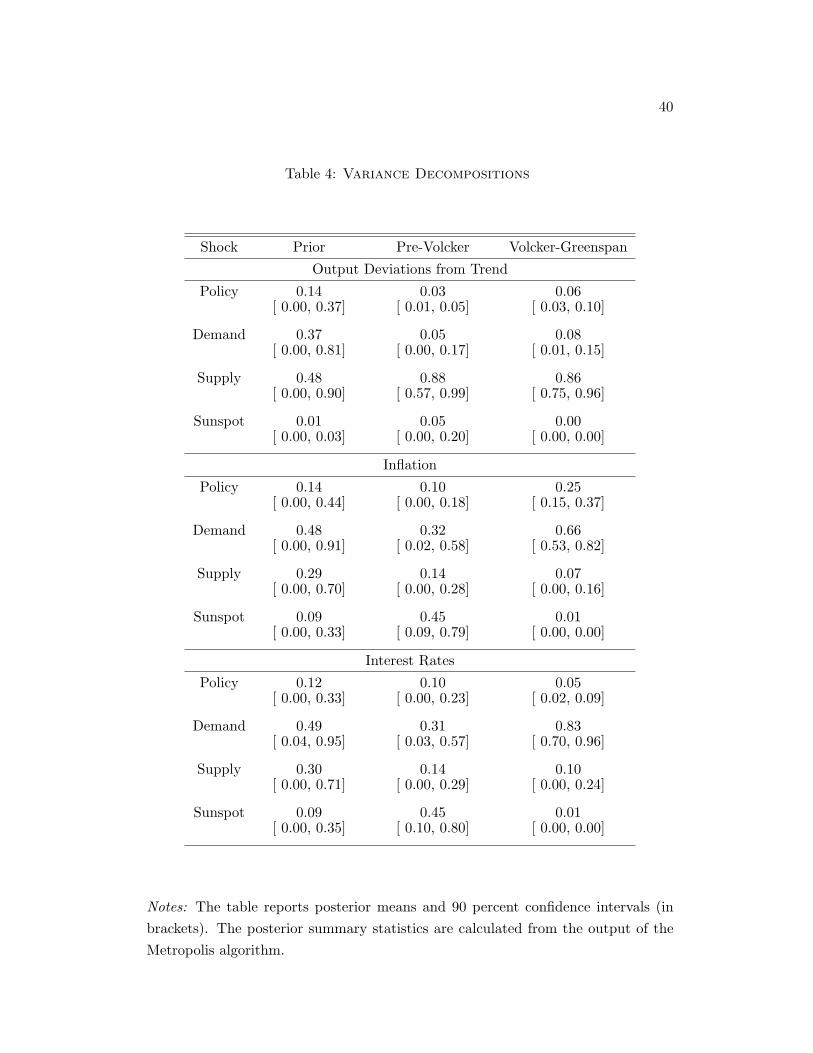
40

Table 4: Variance Decompositions

Shock Prior Pre-Volcker Volcker-Greenspan

Output Deviations from Trend

Policy 0.14 0.03 0.06[ 0.00, 0.37] [ 0.01, 0.05] [ 0.03, 0.10]

Demand 0.37 0.05 0.08[ 0.00, 0.81] [ 0.00, 0.17] [ 0.01, 0.15]

Supply 0.48 0.88 0.86[ 0.00, 0.90] [ 0.57, 0.99] [ 0.75, 0.96]

Sunspot 0.01 0.05 0.00[ 0.00, 0.03] [ 0.00, 0.20] [ 0.00, 0.00]

Inflation

Policy 0.14 0.10 0.25[ 0.00, 0.44] [ 0.00, 0.18] [ 0.15, 0.37]

Demand 0.48 0.32 0.66[ 0.00, 0.91] [ 0.02, 0.58] [ 0.53, 0.82]

Supply 0.29 0.14 0.07[ 0.00, 0.70] [ 0.00, 0.28] [ 0.00, 0.16]

Sunspot 0.09 0.45 0.01[ 0.00, 0.33] [ 0.09, 0.79] [ 0.00, 0.00]

Interest Rates

Policy 0.12 0.10 0.05[ 0.00, 0.33] [ 0.00, 0.23] [ 0.02, 0.09]

Demand 0.49 0.31 0.83[ 0.04, 0.95] [ 0.03, 0.57] [ 0.70, 0.96]

Supply 0.30 0.14 0.10[ 0.00, 0.71] [ 0.00, 0.29] [ 0.00, 0.24]

Sunspot 0.09 0.45 0.01[ 0.00, 0.35] [ 0.10, 0.80] [ 0.00, 0.00]

Notes: The table reports posterior means and 90 percent confidence intervals (inbrackets). The posterior summary statistics are calculated from the output of theMetropolis algorithm.

41

Figure 1: Impulse Responses: Pre-Volcker

Notes: Figure depicts posterior means (solid lines) and pointwise 90% posterior

confidence intervals (dashed lines) for impulse responses of output, inflation, and

the nominal interest rate to one-standard deviation orthogonalized shocks.

42

Figure 2: Impulse Responses: Volcker-Greenspan

Notes: Figure depicts posterior means (solid lines) and pointwise 90% posterior

confidence intervals (dashed lines) for impulse responses of output, inflation, and

the nominal interest rate to one-standard deviation orthogonalized shocks.

43

Figure 3: Determinacy vs Indeterminacy, Pre-Volcker

Notes: Figure depicts posterior mean of the indeterminacy region (solid lines) and

posterior mean of the determinacy region (dashed lines) for impulse responses of

output, inflation, and the nominal interest rate to one-standard deviation orthogo-

nalized shocks.