
Picos Documentation - KOBV fileTakustraße 7 D-14195 Berlin-Dahlem Germany Konrad-Zuse-Zentrum für...
72
Takustraße 7 D-14195 Berlin-Dahlem Germany Konrad-Zuse-Zentrum für Informationstechnik Berlin GUILLAUME S AGNOL Picos Documentation Release 0.1.1 ZIB-Report 12-48 (December 2012)
Transcript of Picos Documentation - KOBV fileTakustraße 7 D-14195 Berlin-Dahlem Germany Konrad-Zuse-Zentrum für...

Takustraße 7D-14195 Berlin-Dahlem
GermanyKonrad-Zuse-Zentrumfür Informationstechnik Berlin
GUILLAUME SAGNOL
Picos DocumentationRelease 0.1.1
ZIB-Report 12-48 (December 2012)

Herausgegeben vomKonrad-Zuse-Zentrum für Informationstechnik BerlinTakustraße 7D-14195 Berlin-Dahlem
Telefon: 030-84185-0Telefax: 030-84185-125
e-mail: [email protected]: http://www.zib.de
ZIB-Report (Print) ISSN 1438-0064ZIB-Report (Internet) ISSN 2192-7782

Picos DocumentationRelease 0.1.1
Guillaume Sagnol
December 10, 2012

CONTENTS
1 Introduction 11.1 First Example . . . . . . . . . . . . . . . . . . . . . . . . . . . . . . . . . . . . . . . . . . . . . 21.2 Solvers . . . . . . . . . . . . . . . . . . . . . . . . . . . . . . . . . . . . . . . . . . . . . . . . 41.3 Requirements . . . . . . . . . . . . . . . . . . . . . . . . . . . . . . . . . . . . . . . . . . . . . 41.4 Installation . . . . . . . . . . . . . . . . . . . . . . . . . . . . . . . . . . . . . . . . . . . . . . 41.5 License . . . . . . . . . . . . . . . . . . . . . . . . . . . . . . . . . . . . . . . . . . . . . . . . 51.6 Author and contributors . . . . . . . . . . . . . . . . . . . . . . . . . . . . . . . . . . . . . . . 5
2 Tutorial 72.1 Variables . . . . . . . . . . . . . . . . . . . . . . . . . . . . . . . . . . . . . . . . . . . . . . . 72.2 Affine Expressions . . . . . . . . . . . . . . . . . . . . . . . . . . . . . . . . . . . . . . . . . . 82.3 Norm of an affine Expression . . . . . . . . . . . . . . . . . . . . . . . . . . . . . . . . . . . . 112.4 Quadratic Expressions . . . . . . . . . . . . . . . . . . . . . . . . . . . . . . . . . . . . . . . . 122.5 Constraints . . . . . . . . . . . . . . . . . . . . . . . . . . . . . . . . . . . . . . . . . . . . . . 122.6 Write a Problem to a file . . . . . . . . . . . . . . . . . . . . . . . . . . . . . . . . . . . . . . . 152.7 Solve a Problem . . . . . . . . . . . . . . . . . . . . . . . . . . . . . . . . . . . . . . . . . . . 16
3 Examples 213.1 Examples from Optimal Experimental Design . . . . . . . . . . . . . . . . . . . . . . . . . . . . 213.2 Cut problems in graphs . . . . . . . . . . . . . . . . . . . . . . . . . . . . . . . . . . . . . . . . 36
4 The PICOS API 494.1 Problem . . . . . . . . . . . . . . . . . . . . . . . . . . . . . . . . . . . . . . . . . . . . . . . . 494.2 picos.tools . . . . . . . . . . . . . . . . . . . . . . . . . . . . . . . . . . . . . . . . . . . . . . 574.3 Expression . . . . . . . . . . . . . . . . . . . . . . . . . . . . . . . . . . . . . . . . . . . . . . 604.4 Constraint . . . . . . . . . . . . . . . . . . . . . . . . . . . . . . . . . . . . . . . . . . . . . . 62
Index 65
i

ii
CHAPTER
ONE
INTRODUCTION
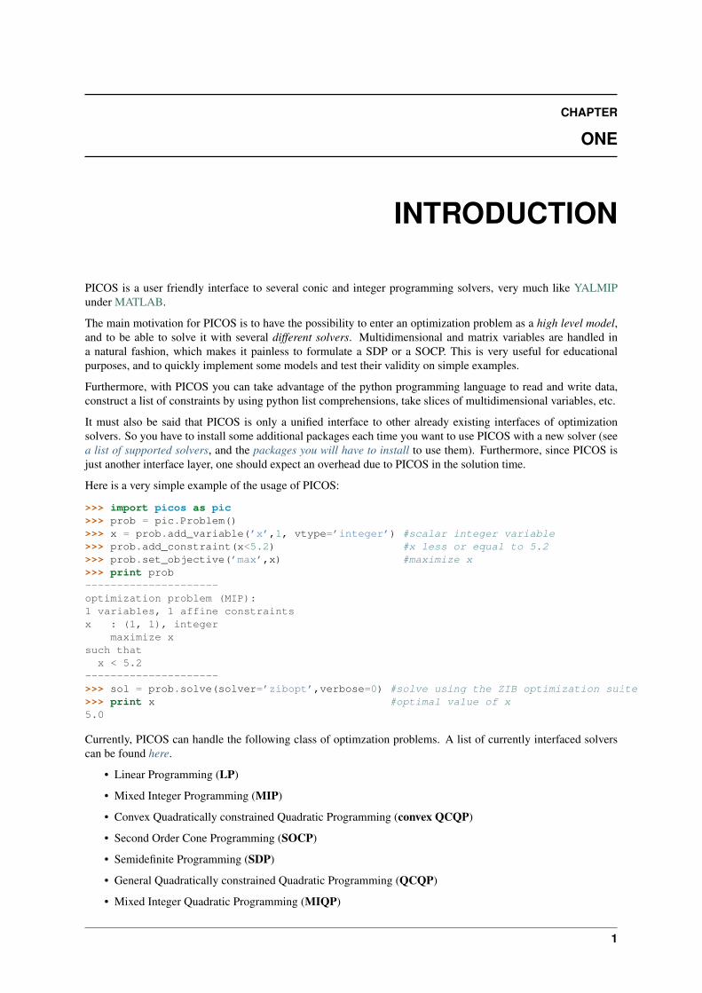
PICOS is a user friendly interface to several conic and integer programming solvers, very much like YALMIPunder MATLAB.
The main motivation for PICOS is to have the possibility to enter an optimization problem as a high level model,and to be able to solve it with several different solvers. Multidimensional and matrix variables are handled ina natural fashion, which makes it painless to formulate a SDP or a SOCP. This is very useful for educationalpurposes, and to quickly implement some models and test their validity on simple examples.
Furthermore, with PICOS you can take advantage of the python programming language to read and write data,construct a list of constraints by using python list comprehensions, take slices of multidimensional variables, etc.
It must also be said that PICOS is only a unified interface to other already existing interfaces of optimizationsolvers. So you have to install some additional packages each time you want to use PICOS with a new solver (seea list of supported solvers, and the packages you will have to install to use them). Furthermore, since PICOS isjust another interface layer, one should expect an overhead due to PICOS in the solution time.
Here is a very simple example of the usage of PICOS:
>>> import picos as pic>>> prob = pic.Problem()>>> x = prob.add_variable(’x’,1, vtype=’integer’) #scalar integer variable>>> prob.add_constraint(x<5.2) #x less or equal to 5.2>>> prob.set_objective(’max’,x) #maximize x>>> print prob---------------------optimization problem (MIP):1 variables, 1 affine constraintsx : (1, 1), integer
maximize xsuch that
x < 5.2--------------------->>> sol = prob.solve(solver=’zibopt’,verbose=0) #solve using the ZIB optimization suite>>> print x #optimal value of x5.0
Currently, PICOS can handle the following class of optimzation problems. A list of currently interfaced solverscan be found here.
• Linear Programming (LP)
• Mixed Integer Programming (MIP)
• Convex Quadratically constrained Quadratic Programming (convex QCQP)
• Second Order Cone Programming (SOCP)
• Semidefinite Programming (SDP)
• General Quadratically constrained Quadratic Programming (QCQP)
• Mixed Integer Quadratic Programming (MIQP)
1

Picos Documentation, Release 0.1.1
There exists a number of similar projects, so we provide a (non-exhausive) list below, explaining their maindifferences with PICOS:
• CVXPY:
This is a python interface that can be used to solve any convex optimization problem. However, CVXPYinterfaces only the open source solver cvxopt for disciplined convex programming (DCP)
• Numberjack:
This python package also provides an interface to the integer programming solver scip, as well as satisfia-bility (SAT) and constraint programming solvers (CP).
• OpenOpt:
This is probably the most complete optimization suite written in python, handling a lot of problem typesand interfacing many opensource and commercial solvers. However, the user has to transform every opti-mization problem into a canonical form himself, and this is what we want to avoid with PICOS.
• puLP:
A user-friendly interface to a bunch of LP and MIP solvers.
• PYOMO:
A modelling language for optimization problems, a la AMPL.
• pyOpt:
A user-friendly package to formulate and solve general nonlinear constrained optimization problems. Sev-eral open-source and commercial solvers are interfaced.
• python-zibopt:
This is a user-friendly interface to the ZIB optimization suite for solving mixed integer programs (MIP).PICOS provides an interface to this interface.
1.1 First Example
We give below a simple example of the use of PICOS, to solve an SOCP which arises in optimal experimentaldesign. More examples can be found here. Given some observation matrices A1, . . . , As, with Ai ∈ Rm×li , anda coefficient matrix K ∈ Rm×r, the problem to solve is:
minimizeµ∈Rs
∀i∈[s], Zi∈Rli×r
s∑i=1
µi
subject tos∑i=1
AiZi = K
∀i ∈ [s], ‖Zi‖F ≤ µi,
where ‖M‖F :=√
traceMMT denotes the Frobenius norm of M . This problem can be entered and solved asfollows with PICOS:
import picos as picimport cvxopt as cvx
#generate dataA = [ cvx.sparse([[1 ,2 ,0 ],
[2 ,0 ,0 ]]),cvx.sparse([[0 ,2 ,2 ]]),cvx.sparse([[0 ,2 ,-1],
[-1,0 ,2 ],
2 Chapter 1. Introduction
Picos Documentation, Release 0.1.1
[0 ,1 ,0 ]])]
K = cvx.sparse([[1 ,1 ,1 ],[1 ,-5,-5]])
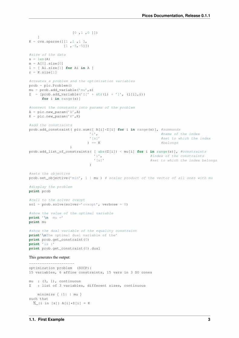
#size of the datas = len(A)m = A[0].size[0]l = [ Ai.size[1] for Ai in A ]r = K.size[1]
#creates a problem and the optimization variablesprob = pic.Problem()mu = prob.add_variable(’mu’,s)Z = [prob.add_variable(’Z[’ + str(i) + ’]’, (l[i],r))
for i in range(s)]
#convert the constants into params of the problemA = pic.new_param(’A’,A)K = pic.new_param(’K’,K)
#add the constraintsprob.add_constraint( pic.sum([ A[i]*Z[i] for i in range(s)], #summands
’i’, #name of the index’[s]’ #set to which the index
) == K #belongs)
prob.add_list_of_constraints( [ abs(Z[i]) < mu[i] for i in range(s)], #constraints’i’, #index of the constraints’[s]’ #set to which the index belongs
)
#sets the objectiveprob.set_objective(’min’, 1 | mu ) # scalar product of the vector of all ones with mu
#display the problemprint prob
#call to the solver cvxoptsol = prob.solve(solver=’cvxopt’, verbose = 0)
#show the value of the optimal variableprint ’\n mu =’print mu
#show the dual variable of the equality constraintprint’\nThe optimal dual variable of the’print prob.get_constraint(0)print ’is :’print prob.get_constraint(0).dual
This generates the output:
---------------------optimization problem (SOCP):15 variables, 6 affine constraints, 15 vars in 3 SO cones
mu : (3, 1), continuousZ : list of 3 variables, different sizes, continuous
minimize ⟨ |1| | mu ⟩such that
Σ_{i in [s]} A[i]*Z[i] = K
1.1. First Example 3
Picos Documentation, Release 0.1.1
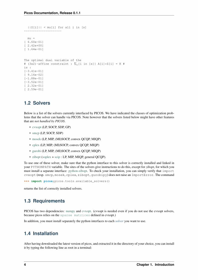
||Z[i]|| < mu[i] for all i in [s]---------------------
mu =[ 6.60e-01][ 2.42e+00][ 1.64e-01]
The optimal dual variable of the# (3x2)-affine constraint : Σ_{i in [s]} A[i]*Z[i] = K #is :[-3.41e-01][ 9.16e-02][-1.88e-01][-3.52e-01][ 2.32e-01][ 2.59e-01]
1.2 Solvers
Below is a list of the solvers currently interfaced by PICOS. We have indicated the classes of optimization prob-lems that the solver can handle via PICOS. Note however that the solvers listed below might have other featuresthat are not handled by PICOS.
• cvxopt (LP, SOCP, SDP, GP)
• smcp (LP, SOCP, SDP)
• mosek (LP, MIP, (MI)SOCP, convex QCQP, MIQP)
• cplex (LP, MIP, (MI)SOCP, convex QCQP, MIQP)
• gurobi (LP, MIP, (MI)SOCP, convex QCQP, MIQP)
• zibopt (soplex + scip : LP, MIP, MIQP, general QCQP).
To use one of these solver, make sure that the python interface to this solver is correctly installed and linked inyour PYTHONPATH variable. The sites of the solvers give instructions to do this, except for zibopt, for which youmust install a separate interface: python-zibopt. To check your installation, you can simply verify that importcvxopt (resp. smcp, mosek, cplex, zibopt, gurobipy) does not raise an ImportError. The command
>>> import picos;picos.tools.available_solvers()
returns the list of correctly installed solvers.
1.3 Requirements
PICOS has two dependencies: numpy and cvxopt. (cvxopt is needed even if you do not use the cvxopt solvers,because picos relies on the sparse matrices defined in cvxopt.)
In addition, you must install separately the python interfaces to each solver you want to use.
1.4 Installation
After having downloaded the latest version of picos, and extracted it in the directory of your choice, you can installit by typing the following line as root in a terminal:
4 Chapter 1. Introduction

Picos Documentation, Release 0.1.1
$ python setup.py install
If you do not have administrator rights, you can also do a local installation of picos with the prefix scheme. Forexample:
$ python setup.py install --prefix ~/python
and make sure that $HOME’/python/lib/python2.x/site-packages/’ is in your PYTHONPATHvariable.
To test your installation, you can run the test file:
$ python picos/test_picos.py
This will generate a table with a list of results for each available solver and class of optimization problems.
1.5 License
This program is free software: you can redistribute it and/or modify it under the terms of the GNU General PublicLicense as published by the Free Software Foundation, either version 3 of the License, or (at your option) anylater version.
This program is distributed in the hope that it will be useful, but WITHOUT ANY WARRANTY; without eventhe implied warranty of MERCHANTABILITY or FITNESS FOR A PARTICULAR PURPOSE. See the GNUGeneral Public License for more details.
You should have received a copy of the GNU General Public License along with this program. If not, see<http://www.gnu.org/licenses/>.
1.6 Author and contributors
• Author: Picos initial author and current primary developer is:
Guillaume Sagnol, <sagnol( a t )zib.de>
• Contributors: People who contributed to Picos and their contributions (in no particular order) are:
– Bertrand Omont
– Elmar Swarat
1.5. License 5

Picos Documentation, Release 0.1.1
6 Chapter 1. Introduction
CHAPTER
TWO
TUTORIAL
First of all, let us import the PICOS module and cvxopt
>>> import picos as pic>>> import cvxopt as cvx
We now generate some arbitrary data, that we will use in this tutorial.
>>> pairs = [(0,2), (1,4), (1,3), (3,2), (0,4),(2,4)] #a list of pairs>>> A = []>>> b = ( [0 ,2 ,0 ,3 ], #a tuple of 5 lists,... [1 ,1 ,0 ,5 ], #each of length 4... [-1,0 ,2 ,4 ],... [0 ,0 ,-2,-1],... [1 ,1 ,0 ,0 ]... )>>> for i in range(5):... A.append(cvx.matrix(range(i-3,i+5),(2,4))) #A is a list of 2x4 matrices>>> D={’Peter’: 12,... ’Bob’ : 4,... ’Betty’: 7,... ’Elisa’: 14... }
Let us now create an instance P of an optimization problem
>>> prob = pic.Problem() #create a Problem instance
2.1 Variables
We will now create the variables of our optimization problem. This is done by calling the methodadd_variable(). This function adds an instance of the class Variable in the dictionaryprob.variables, and returns a reference to the freshly added variable. As we will next see, we can usethis Variable to form affine and quadratic expressions.
>>> t = prob.add_variable(’t’,1) #a scalar>>> x = prob.add_variable(’x’,4) #a column vector>>> Y = prob.add_variable(’Y’,(2,4)) #a matrix>>> Z = []>>> for i in range(5):... Z.append( prob.add_variable(’Z[{0}]’.format(i),(4,2)) )# a list of 5 matrices>>> w={}>>> for p in pairs: #a dictionary of (scalar) binary variables, indexed by our pairs... w[p] = prob.add_variable(’w[{0}]’.format(p),1 , vtype=’binary’)
Now, if we try to display a variable, here is what we get:
7
Picos Documentation, Release 0.1.1
>>> w[2,4]# variable w[(2, 4)]:(1 x 1),binary #>>> Y# variable Y:(2 x 4),continuous #
Also note the use of the attributes name, value, size, and vtype:
>>> w[2,4].vtype’binary’>>> x.vtype’continuous’>>> x.vtype=’integer’>>> x# variable x:(4 x 1),integer #>>> x.size(4, 1)>>> Z[1].value = A[0].T>>> Z[0].is_valued()False>>> Z[1].is_valued()True>>> Z[2].name’Z[2]’
2.2 Affine Expressions
We will now use our variables to create some affine expressions, which are stored as instance of the classAffinExp, and will be the core to define an optimization problem. Most python operators have been over-loaded to work with instances of AffinExp (a list of available overloaded operators can be found in the doc ofAffinExp). For example, you can form the sum of two variables by writing:
>>> Z[0]+Z[3]# (4 x 2)-affine expression: Z[0] + Z[3] #
The transposition of an affine expression is done by appending .T:
>>> x# variable x:(4 x 1),integer #>>> x.T# (1 x 4)-affine expression: x.T #
2.2.1 Parameters as constant affine expressions
It is also possible to form affine expressions by using parameters stored in data structures such as a list or acvxopt matrix (In fact, any type that is recognizable by the function _retrieve_matrix()).
>>> x + b[0]# (4 x 1)-affine expression: x + [ 4 x 1 MAT ] #>>> x.T + b[0]# (1 x 4)-affine expression: x.T + [ 1 x 4 MAT ] #>>> A[0] * Z[0] + A[4] * Z[4]# (2 x 2)-affine expression: [ 2 x 4 MAT ]*Z[0] + [ 2 x 4 MAT ]*Z[4] #
In the above example, you see that the list b[0] was correctly converted into a 4×1 vector in the first expression,and into a 1× 4 vector in the second one. This is because the overloaded operators always try to convert the datainto matrices of the appropriate size.
If you want to have better-looking string representations of your affine expressions, you will need to convert theparameters into constant affine expressions. This can be done thanks to the function new_param():
8 Chapter 2. Tutorial

Picos Documentation, Release 0.1.1
>>> A = pic.new_param(’A’,A) #list of constant affine expressions... # [A[0],...,A[4]]>>> b = pic.new_param(’b’,b) #list of constant affine expressions... # [b[0],...,b[4]]>>> D = pic.new_param(’D’,D) #dictionary of constant AffExpr,... # indexed by ’Peter’, ’Bob’, ...>>> alpha = pic.new_param(’alpha’,12) #a scalar parameter
>>> alpha# (1 x 1)-affine expression: alpha #>>> D[’Betty’]# (1 x 1)-affine expression: D[Betty] #>>> b[# (4 x 1)-affine expression: b[0] #,# (4 x 1)-affine expression: b[1] #,# (4 x 1)-affine expression: b[2] #,# (4 x 1)-affine expression: b[3] #,# (4 x 1)-affine expression: b[4] #]
>>> print b[0][ 0.00e+00][ 2.00e+00][ 0.00e+00][ 3.00e+00]
The above example also illustrates that when a valued affine expression exp is printed, it is its value that is dis-played. For a non-valued affine expression, __repr__ and __str__ produce the same result, a string of the form ’#(size)-affine expression: string-representation #’. Note that the constant affine expres-sions, as b[0] in the above example, are always valued. To assign a value to a non-constant AffinExp, youmust set the value property of every variable involved in the affine expression.
>>> x_minus_1 = x - 1 #note that 1 is recognized as the>>> x_minus_1 #(4x1)-vector with all ones# (4 x 1)-affine expression: x -|1| #>>> print x_minus_1# (4 x 1)-affine expression: x -|1| #>>> x_minus_1.is_valued()False>>> x.value = [0,1,2,-1]>>> x_minus_1.is_valued()True>>> print x_minus_1[-1.00e+00][ 0.00e+00][ 1.00e+00][-2.00e+00]
We also point out that new_param() converts lists into vectors and lists of lists into matrices (given in rowmajor order). In contrast, tuples are converted into list of affine expressions:
>>> pic.new_param(’vect’,[1,2,3]) # a vector of dimension 3# (3 x 1)-affine expression: vect #>>> pic.new_param(’mat’,[[1,2,3],[4,5,6]]) # a (2x3)-matrix# (2 x 3)-affine expression: mat #>>> pic.new_param(’list_of_scalars’,(1,2,3)) # a list of 3 scalar parameters[# (1 x 1)-affine expression: list_of_scalars[0] #,# (1 x 1)-affine expression: list_of_scalars[1] #,# (1 x 1)-affine expression: list_of_scalars[2] #]
>>> pic.new_param(’list_of_vectors’,([1,2,3],[4,5,6])) # a list of 2 vector parameters[# (3 x 1)-affine expression: list_of_vectors[0] #,# (3 x 1)-affine expression: list_of_vectors[1] #]
2.2. Affine Expressions 9
Picos Documentation, Release 0.1.1
2.2.2 Overloaded operators
OK, so now we have some variables (t, x, w, Y, and Z) and some parameters (A, b, D and alpha). Let us createsome affine expressions with them.
>>> A[0] * Z[0] #left multiplication# (2 x 2)-affine expression: A[0]*Z[0] #>>> Z[0] * A[0] #right multiplication# (4 x 4)-affine expression: Z[0]*A[0] #>>> A[1] * Z[0] * A[2] #left and right multiplication# (2 x 4)-affine expression: A[1]*Z[0]*A[2] #>>> alpha*Y #scalar multiplication# (2 x 4)-affine expression: alpha*Y #>>> t/b[1][3] - D[’Bob’] #division by a scalar and substraction# (1 x 1)-affine expression: t / b[1][3] -D[Bob] #>>> ( b[2] | x ) #dot product# (1 x 1)-affine expression: ⟨ b[2] | x ⟩ #>>> ( A[3] | Y ) #generalized dot product for matrices:
# (A|B)=trace(A*B.T)# (1 x 1)-affine expression: ⟨ A[3] | Y ⟩ #
We can also take some subelements of affine expressions, by using the standard syntax of python slices:
>>> b[1][1:3] #2d and 3rd elements of b[1]# (2 x 1)-affine expression: b[1][1:3] #>>> Y[1,:] #2d row of Y# (1 x 4)-affine expression: Y[1,:] #>>> x[-1] #last element of x# (1 x 1)-affine expression: x[-1] #>>> A[2][:,1:3]*Y[:,-2::-2] #extended slicing with (negative) steps# (2 x 2)-affine expression: A[2][:,1:3]*( Y[:,-2::-2] ) #
In the last example, we keep only the second and third columns of A[2], and the columns of Ywith an even index,considered in the reverse order. To concatenate affine expressions, the operators // and & have been overloaded:
>>> (b[1] & b[2] & x & A[0].T*A[0]*x) // x.T #vertical (//) and horizontal (&) concat.# (5 x 4)-affine expression: [b[1],b[2],x,A[0].T*A[0]*x;x.T] #
When a scalar is added/substracted to a matrix or a vector, we interprete it as an elementwise addition of the scalarto every element of the matrix or vector.
>>> 5*x - alpha# (4 x 1)-affine expression: 5*x + |-alpha| #
Warning: Note that the string representation ’|-alpha|’ does not stand for the absolute value of -alpha,but for the vector whose all terms are -alpha.
2.2.3 Summing Affine Expressions
You can take the advantage of python syntax to create sums of affine expressions:
>>> sum([A[i]*Z[i] for i in range(5)])# (2 x 2)-affine expression: A[0]*Z[0] + A[1]*Z[1] + A[2]*Z[2] + A[3]*Z[3] + A[4]*Z[4] #
This works, but you might have very long string representations if there are a lot of summands. So you’d betteruse the function picos.sum()):
>>> pic.sum([A[i]*Z[i] for i in range(5)],’i’,’[5]’)# (2 x 2)-affine expression: Σ_{i in [5]} A[i]*Z[i] #
It is also possible to sum over several indices
10 Chapter 2. Tutorial
Picos Documentation, Release 0.1.1
>>> pic.sum([A[i][1,j] + b[j].T*Z[i] for i in range(5) for j in range(4)],... [’i’,’j’],’[5]x[4]’)# (1 x 2)-affine expression: Σ_{i,j in [5]x[4]} |A[i][1,j]| + b[j].T*Z[i] #
A more complicated example, given in two variants: in the first one, p is a tuple index representing a pair, whilein the second case we explicitely say that the pairs are of the form (p0,p1):
>>> pic.sum([w[p]*b[p[1]-1][p[0]] for p in pairs],(’p’,2),’pairs’)# (1 x 1)-affine expression: Σ_{p in pairs} w[p]*b[p__1-1][p__0] #>>> pic.sum([w[p0,p1]*b[p1-1][p0] for (p0,p1) in pairs],[’p0’,’p1’],’pairs’)# (1 x 1)-affine expression: Σ_{p0,p1 in pairs} w[(p0, p1)]*b[p1-1][p0] #
It is also possible to sum over string indices (see the documentation of sum()):
>>> pic.sum([D[name] for name in D],’name’,’people_list’)# (1 x 1)-affine expression: Σ_{name in people_list} D[name] #
2.2.4 Objective function
The objective function of the problem can be defined with the function set_objective(). Its first argumentshould be ’max’, ’min’ or ’find’ (for feasibility problems), and the second argument should be a scalarexpression:
>>> prob.set_objective(’max’,( A[0] | Y )-t)>>> print prob---------------------optimization problem (MIP):59 variables, 0 affine constraints
w : dict of 6 variables, (1, 1), binaryZ : list of 5 variables, (4, 2), continuoust : (1, 1), continuousY : (2, 4), continuousx : (4, 1), integer
maximize ⟨ A[0] | Y ⟩ -tsuch that
[]---------------------
With this example, you see what happens when a problem is printed: the list of optimization variables is displayed,then the objective function and finally a list of constraints (in the case above, there is no constraint).
2.3 Norm of an affine Expression
The norm of an affine expression is an overload of the abs() function. If x is an affine expression, abs(x) isits Euclidean norm
√xTx.
>>> abs(x)# norm of a (4 x 1)- expression: ||x|| #
In the case where the affine expression is a matrix, abs() returns its Frobenius norm, defined as ‖M‖F :=√trace(MTM).
>>> abs(Z[1]-2*A[0].T)# norm of a (4 x 2)- expression: ||Z[1] -2*A[0].T|| #
Note that the absolute value of a scalar expression is stored as a norm:
2.3. Norm of an affine Expression 11

Picos Documentation, Release 0.1.1
>>> abs(t)# norm of a (1 x 1)- expression: ||t|| #
However, a scalar constraint of the form |aTx+ b| ≤ cTx+ d is handled as two linear constraints by PICOS, andso a problem with the latter constraint can be solved even if you do not have a SOCP solver available. Besides,note that the string representation of an absolute value uses the double bar notation. (Recall that the single barnotation |t| is used to denote the vector whose all values are t).
2.4 Quadratic Expressions
Quadratic expressions can be formed in several ways:
>>> t**2 - x[1]*x[2] + 2*t - alpha #sum of linear and... #quadratic terms#quadratic expression: t**2 -x[1]*x[2] + 2.0*t -alpha #>>> (x[1]-2) * (t+4) #product of two AffExpr#quadratic expression: ( x[1] -2.0 )*( t + 4.0 ) #>>> Y[0,:]*x #Row vector multiplied... #by column vector#quadratic expression: Y[0,:]*x #>>> (x +2 | Z[1][:,1]) #dot product of 2 AffExpr#quadratic expression: ⟨ x + |2.0| | Z[1][:,1] ⟩ #>>> abs(x)**2 #recall that abs(x) is... #the euclidean norm of x#quadratic expression: ||x||**2 #>>> (t & alpha) * A[1] * x #quadratic form#quadratic expression: [t,alpha]*A[1]*x #
It is not possible (yet) to make a multidimensional quadratic expression.
2.5 Constraints
A constraint takes the form of two expressions separated by a relation operator.
2.5.1 Linear (in)equalities
Linear (in)equalities are understood elementwise. The strict operators < and > denote weak inequalities (lessor equal than and larger or equal than). For example:
>>> (1|x) < 2 #sum of the x[i] < or = than 2# (1x1)-affine constraint: ⟨ |1| | x ⟩ < 2.0 #>>> Z[0] * A[0] > b[1]*b[2].T #A 4x4-elementwise inequality# (4x4)-affine constraint: Z[0]*A[0] > b[1]*b[2].T #>>> pic.sum([A[i]*Z[i] for i in range(5)],’i’,’[5]’) == 0 #A 2x2 equality;... #The RHS is the all-zero matrix.# (2x2)-affine constraint: Σ_{i in [5]} A[i]*Z[i] = |0| #
Constraints can be added in the problem with the function add_constraint():
>>> for i in range(1,5):... prob.add_constraint(Z[i]==Z[i-1]+Y.T)>>> print prob---------------------optimization problem (MIP):59 variables, 32 affine constraints
w : dict of 6 variables, (1, 1), binary
12 Chapter 2. Tutorial

Picos Documentation, Release 0.1.1
Z : list of 5 variables, (4, 2), continuoust : (1, 1), continuousY : (2, 4), continuousx : (4, 1), integer
maximize ⟨ A[0] | Y ⟩ -tsuch that
Z[1] = Z[0] + Y.TZ[2] = Z[1] + Y.TZ[3] = Z[2] + Y.TZ[4] = Z[3] + Y.T
---------------------
The constraints of the problem can then be accessed with the function get_constraint():
>>> prob.get_constraint(2) #constraints are numbered from 0# (4x2)-affine constraint: Z[3] = Z[2] + Y.T #
An alternative is to pass the constraint with the option ret = True, which has the effect to return a referenceto the constraint you want to add. In particular, this reference can be useful to access the optimal dual variable ofthe constraint, once the problem will have been solved.
>>> mycons = prob.add_constraint(Z[4]+Z[0] == Y.T, ret = True)>>> print mycons# (4x2)-affine constraint : Z[4] + Z[0] = Y.T #
2.5.2 Groupping constraints
In order to have a more compact string representation of the problem, it is advised to use the functionadd_list_of_constraints(), which works similarly as the function sum().
>>> prob.remove_all_constraints() #we first remove the 4 constraints precedently added>>> prob.add_constraint(Y>0) #a single constraint>>> prob.add_list_of_constraints([Z[i]==Z[i-1]+Y.T for i in range(1,5)],’i’,’1...4’)... #the same list of constraints as above>>> print prob---------------------optimization problem (MIP):59 variables, 40 affine constraints
w : dict of 6 variables, (1, 1), binaryZ : list of 5 variables, (4, 2), continuoust : (1, 1), continuousY : (2, 4), continuousx : (4, 1), integer
maximize ⟨ A[0] | Y ⟩ -tsuch that
Y > |0|Z[i] = Z[i-1] + Y.T for all i in 1...4
---------------------
Now, the constraint Z[3] = Z[2] + Y.T, which has been entered in 4th position, can either be accessed byprob.get_constraint(3) (3 because constraints are numbered from 0), or by
>>> prob.get_constraint((1,2))# (4x2)-affine constraint: Z[3] = Z[2] + Y.T #
where (1,2) means the 3rd constraint of the 2d group of constraints, with zero-based numbering.
Similarly, the constraint Y > |0| can be accessed by prob.get_constraint(0) (firstconstraint), prob.get_constraint((0,0)) (first constraint of the first group), orprob.get_constraint((0,)) (unique constraint of the first group).
2.5. Constraints 13
Picos Documentation, Release 0.1.1
2.5.3 Quadratic constraints
Quadratic inequalities are entered in the following way:
>>> t**2 > 2*t - alpha + x[1]*x[2]#Quadratic constraint -t**2 + 2.0*t -alpha + x[1]*x[2] < 0 #>>> (t & alpha) * A[1] * x + (x +2 | Z[1][:,1]) < 3*(1|Y)-alpha#Quadratic constraint [t,alpha]*A[1]*x + ⟨ x + |2.0| | Z[1][:,1] ⟩ -(3.0*⟨ |1| | Y ⟩ -alpha) < 0 #
Note that PICOS does not check the convexity of convex constraints. It is the solver which will raise an Exceptionif it does not support non-convex quadratics.
2.5.4 Second Order Cone Constraints
There are two types of second order cone constraints supported in PICOS.
• The constraints of the type ‖x‖ ≤ t, where t is a scalar affine expression and x is a multidimensional affineexpression (possibly a matrix, in which case the norm is Frobenius). This inequality forces the vector [x; t]to belong to a Lorrentz-Cone (also called ice-cream cone)
• The constraints of the type ‖x‖2 ≤ tu, t ≥ 0, where t and u are scalar affine expressions and x is amultidimensional affine expression, which constrain the vector [x, t, u] inside a rotated version of the Lorretzcone. When a constraint of the form abs(x)**2 < t*u is passed to PICOS, it is implicitely assumedthat t is nonnegative, and the constraint is handled as the equivalent, standard ice-cream cone constraint‖ [2x, t− u] ‖ ≤ t+ u.
A few examples:
>>> abs(x) < (2|x-1) #A simple ice-cream cone constraint# (4x1)-SOC constraint: ||x|| < ⟨ |2.0| | x -|1| ⟩ #>>> abs(Y+Z[0].T) < t+alpha #SOC constraint with Frobenius norm# (2x4)-SOC constraint: ||Y + Z[0].T|| < t + alpha #>>> abs(Z[1][:,0])**2 < (2*t-alpha)*(x[2]-x[-1]) #Rotated SOC constraint# (4x1)-Rotated SOC constraint: ||Z[1][:,0]||^2 < ( 2.0*t -alpha)( x[2] -(x[-1])) #>>> t**2 < D[’Elisa’]+t #t**2 is understood as... #the squared norm of [t]# (1x1)-Rotated SOC constraint: ||t||^2 < D[Elisa] + t #>>> 1 < (t-1)*(x[2]+x[3]) #1 is understood as... #the squared norm of [1]# (1x1)-Rotated SOC constraint: 1.0 < ( t -1.0)( x[2] + x[3]) #
2.5.5 Semidefinite Constraints
Linear matrix inequalities (LMI) can be entered thanks to an overload of the operators << and >>. For example,the LMI
3∑i=0
xibibTi � b4bT4 ,
where � is used to denote the Löwner ordering, is passed to PICOS by writing:
>>> pic.sum([x[i]*b[i]*b[i].T for i in range(4)],’i’,’0...3’) >> b[4]*b[4].T# (4x4)-LMI constraint Σ_{i in 0...3} x[i]*b[i]*b[i].T � b[4]*b[4].T #
Note the difference with
>>> pic.sum([x[i]*b[i]*b[i].T for i in range(4)],’i’,’0...3’) > b[4]*b[4].T# (4x4)-affine constraint: Σ_{i in 0...3} x[i]*b[i]*b[i].T > b[4]*b[4].T #
which yields an elementwise inequality.
14 Chapter 2. Tutorial

Picos Documentation, Release 0.1.1
For convenience, it is possible to add a symmetric matrix variable X, by specifying the optionvtype=symmetric. This has the effect to store all the affine expressions which depend on X as a functionof its lower triangular elements only.
>>> sdp = pic.Problem()>>> X = sdp.add_variable(’X’,(4,4),vtype=’symmetric’)>>> sdp.add_constraint(X >> 0)>>> print sdp---------------------optimization problem (SDP):10 variables, 0 affine constraints, 10 vars in 1 SD cones
X : (4, 4), symmetric
find varssuch that
X � |0|---------------------
In this example, you see indeed that the problem has 10=(4*5)/2 variables, which correspond to the lower trian-gular elements of X.
Warning: When a constraint of the form A >> B is passed to PICOS, it is not assumed that A-B is symmet-ric. Instead, the symmetric matrix whose lower triangular elements are those of A-B is forced to be positivesemidefnite. So, in the cases where A-B is not implicitely forced to be symmetric, you should add a constraintof the form A-B==(A-B).T in the problem.
2.6 Write a Problem to a file
It is possible to write a problem to a file, thanks to the function write_to_file(). Several file formats andfile writers are available, have a look at the doc of write_to_file() for more explanations.
Below is a hello world example, which writes a simple MIP to a .lp file:
import picos as picprob = pic.Problem()y = prob.add_variable(’y’,1, vtype=’integer’)x = prob.add_variable(’x’,1)prob.add_constraint(x>1.5)prob.add_constraint(y-x>0.7)prob.set_objective(’min’,y)#let first picos display the problemprint probprint#now write the problem to a .lp file...prob.write_to_file(’helloworld.lp’)print#and display the content of the freshly created file:print open(’helloworld.lp’).read()
Generated output:
---------------------optimization problem (MIP):2 variables, 2 affine constraints
y : (1, 1), integerx : (1, 1), continuous
minimize ysuch that
2.6. Write a Problem to a file 15

Picos Documentation, Release 0.1.1
x > 1.5y -x > 0.7---------------------
writing problem in helloworld.lp...done.
\* file helloworld.lp generated by picos*\Minimizeobj : 1 ySubject Toin0 : -1 y+ 1 x <= -0.7Boundsy free1.5 <= x<= +infGeneralsyBinariesEnd
2.7 Solve a Problem
To solve a problem, you have to use the method solve() of the class Problem. This methodaccepts several options. In particular the solver can be specified by passing an option of the formsolver=’solver_name’. For a list of available parameters with their default values, see the doc of thefunction set_all_options_to_default().
Once a problem has been solved, the optimal values of the variables are accessible with the value property.Depending on the solver, you can also obtain the slack and the optimal dual variables of the constraints thanks tothe properties dual and slack of the class Constraint. See the doc of dual for more explanations on thedual variables for second order cone programs (SOCP) and semidefinite programs (SDP).
The class Problem also has two interesting properties: type, which indicates the class of the optimizationproblem (‘LP’, ‘SOCP’, ‘MIP’, ‘SDP’,...), and status, which indicates if the problem has been solved (thedefault is ’unsolved’; after a call to solve() this property can take the value of any code returned by asolver, such as ’optimal’, ’unbounded’, ’near-optimal’, ’primal infeasible’, ’unknown’,...).
Below is a simple example, to solve the linear programm:
minimizex∈R2
0.5x1 + x2
subject to x1 ≥ x2[1 01 1
]x ≤
[34
].
More examples can be found here.
P = pic.Problem()A = pic.new_param(’A’, cvx.matrix([[1,1],[0,1]]) )x = P.add_variable(’x’,2)P.add_constraint(x[0]>x[1])P.add_constraint(A*x<[3,4])objective = 0.5 * x[0] + x[1]P.set_objective(’max’, objective)
#display the problem and solve itprint Pprint ’type: ’+P.typeprint ’status: ’+P.statusP.solve(solver=’cvxopt’,verbose=False)print ’status: ’+P.status
16 Chapter 2. Tutorial

Picos Documentation, Release 0.1.1
#--------------------## objective value ##--------------------#
print ’the optimal value of this problem is:’print P.obj_value() #"print objective" would also work
#--------------------## optimal variable ##--------------------#x_opt = x.valueprint ’The solution of the problem is:’print x_opt #"print x" would also work, since x is now valuedprint
#--------------------## slacks and duals ##--------------------#c0=P.get_constraint(0)print ’The dual of the constraint’print c0print ’is:’print c0.dualprint ’And its slack is:’print c0.slackprint
c1=P.get_constraint(1)print ’The dual of the constraint’print c1print ’is:’print c1.dualprint ’And its slack is:’print c1.slack
---------------------optimization problem (LP):2 variables, 3 affine constraints
x : (2, 1), continuous
maximize 0.5*x[0] + x[1]such that
x[0] > x[1]A*x < [ 2 x 1 MAT ]
---------------------type: LPstatus: unsolvedstatus: optimal
the optimal value of this problem is:3.0000000002The solution of the problem is:[ 2.00e+00][ 2.00e+00]
The dual of the constraint# (1x1)-affine constraint : x[0] > x[1] #is:[ 2.50e-01]
2.7. Solve a Problem 17
Picos Documentation, Release 0.1.1
And its slack is:[ 1.83e-09]
The dual of the constraint# (2x1)-affine constraint : A*x < [ 2 x 1 MAT ] #is:[ 4.56e-10][ 7.50e-01]
And its slack is:[ 1.00e+00][-8.71e-10]
2.7.1 A note on dual variables
For second order cone constraints of the form ‖x‖ ≤ t, where x is a vector of dimension n, the dual variable is avector of dimension n+ 1 of the form [λ; z], where the n− dimensional vector z satisfies ‖z‖ ≤ λ.
Since rotated second order cone constraints of the form ‖x‖2 ≤ tu, t ≥ 0, are handled as the equivalent ice-creamconstraint ‖[2x; t− u]‖ ≤ t+ u, the dual is given with respect to this reformulated, standard SOC constraint.
In general, a linear problem with second order cone constraints (both standard and rotated) and semidefiniteconstraints can be written under the form:
minimizex∈Rn
cTx
subject to Aex+ be = 0Alx+ bl ≤ 0
‖Asix+ bsi ‖ ≤ f si
Tx+ dsi , ∀i ∈ I‖Arjx+ br
j‖2 ≤ (fr1jTx+ dr1j )(fr2j
Tx+ dr2j ), ∀j ∈ J
0 ≤ fr1jTx+ dr1j , ∀j ∈ J∑n
i=1 xiMi �M0
where
• c,{f si}i∈I ,
{fr1j}j∈J ,
{fr2j}j∈J are vectors of dimension n;
•{dsi}i∈I ,
{dr1j}j∈J ,
{dr2j}j∈J are scalars;
•{bsi
}i∈I are vectors of dimension nsi and
{Asi}i∈I are matrices of size nsi × n;
•{brj
}j∈J are vectors of dimension nrj and
{Arj}j∈J are matrices of size nrj × n;
• be is a vector of dimension ne and Ae is a matrix of size ne × n;
• bl is a vector of dimension nl and Al is a matrix of size nl × n;
•{Mk
}k=0,...,n
are m×m symmetric matrices (Mk ∈: math :mathbb{S}_m‘).
Its dual problem can be written as:
maximize beTµe + blTµl +∑i∈I(bsiT zsi − dsiλi
)+∑j∈J
(brjT zrj − d
r1j αj − d
r2j βj
)+ 〈M0, X〉
subject to c+AeTµe +AlTµl +
∑i∈I(Asi
T zsi − λif si)+∑j∈J
(Arj
T zrj − αjfr1j − βjf
r2j
)=M•X
µl ≥ 0‖zsi ‖ ≤ λi, ∀i ∈ I‖zrj‖2 ≤ 4αjβj , ∀j ∈ J0 ≤ αj , ∀j ∈ JX � 0
whereM•X stands for the vector of dimension n with 〈Mi, X〉 on the i th coordinate, and the dual variables are
• µe ∈ Rne
• µl ∈ Rnl
18 Chapter 2. Tutorial
Picos Documentation, Release 0.1.1
• zsi ∈ Rnsi , ∀i ∈ I
• λi ∈ R, ∀i ∈ I
• zrj ∈ Rnrj , ∀j ∈ J
• (αj , βj) ∈ R2, ∀j ∈ J
• X ∈ SmWhen quering the dual of a constraint of the above primal problem, picos will return
• µe for the constraint Aex+ be = 0;
• µl for the constraint Alx+ bl ≥ 0;
• The (nsi + 1)− dimensional vector µsi := [λi; zsi ] for the constraint
‖Asix+ bsi ‖ ≤ f si
Tx+ dsi ;
• The (nrj + 2)− dimensional vector µrj = 12 [ (βj + αj); z
rj ; (βj − αj) ] for the constraint
‖Arjx+ brj‖2 ≤ (fr1j
Tx+ dr1j )(fr2j
Tx+ dr2j )
In other words, if the dual vector returned by picos is of the form µrj = [σ1j ;uj;σ
2j ], where uj is of
dimension nrj , then the dual variables of the rotated conic constraint are αj = σ1j − σ2
j , βj = σ1j + σ2
j andzrj = 2uj;
• The symmetric positive definite matrix X for the constraint∑ni=1 xiMi �M0.
2.7. Solve a Problem 19

Picos Documentation, Release 0.1.1
20 Chapter 2. Tutorial

CHAPTER
THREE
EXAMPLES
3.1 Examples from Optimal Experimental Design
Optimal experimental design is a theory at the interface of statistics and optimization, which studies how toallocate some experimental effort within a set of available expeiments. The goal is to allow for the best possibleestimation of an unknown parameter θ. In what follows, we assume the standard linear model with multiresponseexperiments: the ith experiment gives a multidimensional observation that can be written as yi = ATi θ+ εi, whereyi is of dimension li, Ai is a m× li− matrix, and the noise vectors εi are i.i.d. with a unit variance.
Several optimization criterions exist, leading to different SDP, SOCP and LP formulations. As such, optimalexperimental design problens are natural examples for problems in conic optimization. For a review of the differentformulations and more references, see [1].
The code below initializes the data used in all the examples of this page. It should be run prior to any of the codespresented in this page.
import cvxopt as cvximport picos as pic
#---------------------------------## First generate some data : ## _ a list of 8 matrices A ## _ a vector c ##---------------------------------#A=[ cvx.matrix([[1,0,0,0,0],
[0,3,0,0,0],[0,0,1,0,0]]),
cvx.matrix([[0,0,2,0,0],[0,1,0,0,0],[0,0,0,1,0]]),
cvx.matrix([[0,0,0,2,0],[4,0,0,0,0],[0,0,1,0,0]]),
cvx.matrix([[1,0,0,0,0],[0,0,2,0,0],[0,0,0,0,4]]),
cvx.matrix([[1,0,2,0,0],[0,3,0,1,2],[0,0,1,2,0]]),
cvx.matrix([[0,1,1,1,0],[0,3,0,1,0],[0,0,2,2,0]]),
cvx.matrix([[1,2,0,0,0],[0,3,3,0,5],[1,0,0,2,0]]),
cvx.matrix([[1,0,3,0,1],[0,3,2,0,0],[1,0,0,2,0]])
21
Picos Documentation, Release 0.1.1
]
c = cvx.matrix([1,2,3,4,5])
3.1.1 c-optimality, multi-response: SOCP
We compute the c-optimal design (c=[1,2,3,4,5]) for the observation matrices A[i].T from the variable Adefined above. The results below suggest that we should allocate 12.8% of the experimental effort on experiment#5, and 87.2% on experiment #7.
Primal Problem
The SOCP for multiresponse c-optimal design is:
minimizeµ∈Rs
∀i∈[s], zi∈Rli
s∑i=1
µi
subject tos∑i=1
Aizi = c
∀i ∈ [s], ‖zi‖2 ≤ µi,
#create the problem, variables and paramsprob_primal_c=pic.Problem()AA=[cvx.sparse(a,tc=’d’) for a in A] #each AA[i].T is a 3 x 5 observation matrixs=len(AA)AA=pic.new_param(’A’,AA)cc=pic.new_param(’c’,c)z=[prob_primal_c.add_variable(’z[’+str(i)+’]’,AA[i].size[1]) for i in range(s)]mu=prob_primal_c.add_variable(’mu’,s)
#define the constraints and objective functionprob_primal_c.add_list_of_constraints(
[abs(z[i])<mu[i] for i in range(s)], #constraints’i’, #index’[s]’ #set to which the index belongs)
prob_primal_c.add_constraint(pic.sum(
[AA[i]*z[i] for i in range(s)], #summands’i’, #index’[s]’ #set to which the index belongs)
== cc )prob_primal_c.set_objective(’min’,1|mu)
#solve the problem and retrieve the optimal weights of the optimal design.print prob_primal_cprob_primal_c.solve(verbose=0,solver=’cvxopt’)
mu=mu.valuew=mu/sum(mu) #normalize mu to get the optimal weightsprintprint ’The optimal deign is:’print w
Generated output:
22 Chapter 3. Examples

Picos Documentation, Release 0.1.1
---------------------optimization problem (SOCP):32 variables, 5 affine constraints, 32 vars in 8 SO cones
z : list of 8 variables, (3, 1), continuousmu : (8, 1), continuous
minimize ⟨ |1| | mu ⟩such that||z[i]|| < mu[i] for all i in [s]Σ_{i in [s]} A[i]*z[i] = c---------------------
The optimal deign is:[...][...][...][...][ 1.28e-01][...][ 8.72e-01][...]
The [...] above indicate a numerical zero entry (i.e., which can be something like 2.84e-10). We use the ellipsis... instead for clarity and compatibility with doctest.
Dual Problem
This is only to check that we obtain the same solution with the dual problem, and to provide one additionalexample in this doc:
maximizeu∈Rm
cTu
subject to ∀i ∈ [s], ‖ATi u‖2 ≤ 1
#create the problem, variables and paramsprob_dual_c=pic.Problem()AA=[cvx.sparse(a,tc=’d’) for a in A] #each AA[i].T is a 3 x 5 observation matrixs=len(AA)AA=pic.new_param(’A’,AA)cc=pic.new_param(’c’,c)u=prob_dual_c.add_variable(’u’,c.size)
#define the constraints and objective functionprob_dual_c.add_list_of_constraints(
[abs(AA[i].T*u)<1 for i in range(s)], #constraints’i’, #index’[s]’ #set to which the index belongs)
prob_dual_c.set_objective(’max’, cc|u)
#solve the problem and retrieve the weights of the optimal designprint prob_dual_cprob_dual_c.solve(verbose=0)
#Lagrangian duals of the SOC constraintsmu = [cons.dual[0] for cons in prob_dual_c.get_constraint((0,))]mu = cvx.matrix(mu)w=mu/sum(mu) #normalize mu to get the optimal weightsprint
3.1. Examples from Optimal Experimental Design 23

Picos Documentation, Release 0.1.1
print ’The optimal deign is:’print w
Generated output:
---------------------optimization problem (SOCP):5 variables, 0 affine constraints, 32 vars in 8 SO cones
u : (5, 1), continuous
maximize ⟨ c | u ⟩such that||A[i].T*u|| < 1 for all i in [s]---------------------
The optimal deign is:[...][...][...][...][ 1.28e-01][...][ 8.72e-01][...]
3.1.2 c-optimality, single-response: LP
When the observation matrices are row vectors (single-response framework), the SOCP above reduces to a simpleLP, because the variables zi are scalar. We solve below the LP for the case where there are 12 available experi-ments, corresponding to the columns of the matrices A[4], A[5], A[6], and A[7] defined in the preambule.
The optimal design allocates 3.37% to experiment #5 (2nd column of A[5]), 27.9% to experiment #7 (1st columnof A[6]), 11.8% to experiment #8 (2nd column of A[6]), 27.6% to experiment #9 (3rd column of A[6]), and29.3% to experiment #11 (2nd column of A[7]).
#create the problem, variables and paramsprob_LP=pic.Problem()AA=[cvx.sparse(a[:,i],tc=’d’) for i in range(3) for a in A[4:]] #12 column vectorss=len(AA)AA=pic.new_param(’A’,AA)cc=pic.new_param(’c’,c)z=[prob_LP.add_variable(’z[’+str(i)+’]’,1) for i in range(s)]mu=prob_LP.add_variable(’mu’,s)
#define the constraints and objective functionprob_LP.add_list_of_constraints(
[abs(z[i])<mu[i] for i in range(s)], #constraints handled as -mu_i < z_i< mu_i’i’, #index’[s]’ #set to which the index belongs)
prob_LP.add_constraint(pic.sum(
[AA[i]*z[i] for i in range(s)], #summands’i’, #index’[s]’ #set to which the index belongs)
== cc )prob_LP.set_objective(’min’,1|mu)
#solve the problem and retrieve the weights of the optimal designprint prob_LP
24 Chapter 3. Examples
Picos Documentation, Release 0.1.1
prob_LP.solve(verbose=0)
mu=mu.valuew=mu/sum(mu) #normalize mu to get the optimal weightsprintprint ’The optimal deign is:’print w
Note that there are no cone constraints, because the constraints of the form |zi| ≤ µi are handled as two inequalitieswhen zi is scalar, so the problem is a LP indeed:---------------------optimization problem (LP):24 variables, 29 affine constraints
z : list of 12 variables, (1, 1), continuousmu : (12, 1), continuous
minimize ⟨ |1| | mu ⟩such that||z[i]|| < mu[i] for all i in [s]Σ_{i in [s]} A[i]*z[i] = c---------------------
The optimal deign is:[...][...][...][...][ 3.37e-02][...][ 2.79e-01][ 1.18e-01][ 2.76e-01][...][ 2.93e-01][...]
3.1.3 SDP formulation of the c-optimal design problem
We give below the SDP for c-optimality, in primal and dual form. You can observe that we obtain the same resultsas with the SOCP presented earlier: 12.8% on experiment #5, and 87.2% on experiment #7.
Primal Problem
The SDP formulation of the c-optimal design problem is:
minimizeµ∈Rs
s∑i=1
µi
subject tos∑i=1
µiAiATi � ccT ,
µ ≥ 0.
#create the problem, variables and paramsprob_SDP_c_primal=pic.Problem()AA=[cvx.sparse(a,tc=’d’) for a in A] #each AA[i].T is a 3 x 5 observation matrixs=len(AA)
3.1. Examples from Optimal Experimental Design 25
Picos Documentation, Release 0.1.1
AA=pic.new_param(’A’,AA)cc=pic.new_param(’c’,c)mu=prob_SDP_c_primal.add_variable(’mu’,s)
#define the constraints and objective functionprob_SDP_c_primal.add_constraint(
pic.sum([mu[i]*AA[i]*AA[i].T for i in range(s)], #summands’i’, #index’[s]’ #set to which the index belongs)>> cc*cc.T )
prob_SDP_c_primal.add_constraint(mu>0)prob_SDP_c_primal.set_objective(’min’,1|mu)
#solve the problem and retrieve the weights of the optimal designprint prob_SDP_c_primalprob_SDP_c_primal.solve(verbose=0)w=mu.valuew=w/sum(w) #normalize mu to get the optimal weightsprintprint ’The optimal deign is:’print w
Generated output:
---------------------optimization problem (SDP):8 variables, 8 affine constraints, 15 vars in 1 SD cones
mu : (8, 1), continuous
minimize ⟨ |1| | mu ⟩such thatΣ_{i in [s]} mu[i]*A[i]*A[i].T � c*c.Tmu > |0|---------------------
The optimal deign is:[...][...][...][...][ 1.28e-01][...][ 8.72e-01][...]
Dual Problem
This is only to check that we obtain the same solution with the dual problem, and to provide one additionalexample in this doc:
maximizeX∈Rm×m
cTXc
subject to ∀i ∈ [s], 〈AiATi , X〉 ≤ 1,
X � 0.
26 Chapter 3. Examples

Picos Documentation, Release 0.1.1
#create the problem, variables and paramsprob_SDP_c_dual=pic.Problem()AA=[cvx.sparse(a,tc=’d’) for a in A] #each AA[i].T is a 3 x 5 observation matrixs=len(AA)AA=pic.new_param(’A’,AA)cc=pic.new_param(’c’,c)m =c.size[0]X=prob_SDP_c_dual.add_variable(’X’,(m,m),vtype=’symmetric’)
#define the constraints and objective functionprob_SDP_c_dual.add_list_of_constraints(
[(AA[i]*AA[i].T | X ) <1 for i in range(s)], #constraints’i’, #index’[s]’ #set to which the index belongs)
prob_SDP_c_dual.add_constraint(X>>0)prob_SDP_c_dual.set_objective(’max’, cc.T*X*cc)
#solve the problem and retrieve the weights of the optimal designprint prob_SDP_c_dualprob_SDP_c_dual.solve(verbose=0,solver=’smcp’)#Lagrangian duals of the SOC constraintsmu = [cons.dual[0] for cons in prob_SDP_c_dual.get_constraint((0,))]mu = cvx.matrix(mu)w=mu/sum(mu) #normalize mu to get the optimal weightsprintprint ’The optimal deign is:’print wprint ’and the optimal positive semidefinite matrix X is’print X
Generated output:
---------------------optimization problem (SDP):15 variables, 8 affine constraints, 15 vars in 1 SD cones
X : (5, 5), symmetric
maximize c.T*X*csuch that⟨ A[i]*A[i].T | X ⟩ < 1.0 for all i in [s]X � |0|---------------------
The optimal deign is:[...][...][...][...][ 1.28e-01][...][ 8.72e-01][...]
and the optimal positive semidefinite matrix X is[ 5.92e-03 8.98e-03 2.82e-03 -3.48e-02 -1.43e-02][ 8.98e-03 1.36e-02 4.27e-03 -5.28e-02 -2.17e-02][ 2.82e-03 4.27e-03 1.34e-03 -1.66e-02 -6.79e-03][-3.48e-02 -5.28e-02 -1.66e-02 2.05e-01 8.39e-02][-1.43e-02 -2.17e-02 -6.79e-03 8.39e-02 3.44e-02]
3.1. Examples from Optimal Experimental Design 27
Picos Documentation, Release 0.1.1
3.1.4 A-optimality: SOCP
We compute the A-optimal design for the observation matrices A[i].T defined in the preambule. The optimaldesign allocates 24.9% on experiment #3, 14.2% on experiment #4, 8.51% on experiment #5, 12.1% on experiment#6, 13.2% on experiment #7, and 27.0% on experiment #8.
[ 2.49e-01] [ 1.42e-01] [ 8.51e-02] [ 1.21e-01] [ 1.32e-01] [ 2.70e-01]
Primal Problem
The SOCP for the A-optimal design problem is:
minimizeµ∈Rs
∀i∈[s], Zi∈Rli×m
s∑i=1
µi
subject tos∑i=1
AiZi = I
∀i ∈ [s], ‖Zi‖F ≤ µi,
#create the problem, variables and paramsprob_primal_A=pic.Problem()AA=[cvx.sparse(a,tc=’d’) for a in A] #each AA[i].T is a 3 x 5 observation matrixs=len(AA)AA=pic.new_param(’A’,AA)Z=[prob_primal_A.add_variable(’Z[’+str(i)+’]’,AA[i].T.size) for i in range(s)]mu=prob_primal_A.add_variable(’mu’,s)
#define the constraints and objective functionprob_primal_A.add_list_of_constraints(
[abs(Z[i])<mu[i] for i in range(s)], #constraints’i’, #index’[s]’ #set to which the index belongs)
prob_primal_A.add_constraint(pic.sum([AA[i]*Z[i] for i in range(s)], #summands’i’, #index’[s]’ #set to which the index belongs)== ’I’ )
prob_primal_A.set_objective(’min’,1|mu)
#solve the problem and retrieve the weights of the optimal designprint prob_primal_Aprob_primal_A.solve(verbose=0)w=mu.valuew=w/sum(w) #normalize mu to get the optimal weightsprintprint ’The optimal deign is:’print w
Generated output:
---------------------optimization problem (SOCP):128 variables, 25 affine constraints, 128 vars in 8 SO cones
Z : list of 8 variables, (3, 5), continuousmu : (8, 1), continuous
28 Chapter 3. Examples
Picos Documentation, Release 0.1.1
minimize ⟨ |1| | mu ⟩such that||Z[i]|| < mu[i] for all i in [s]Σ_{i in [s]} A[i]*Z[i] = I---------------------
The optimal deign is:[...][...][ 2.49e-01][ 1.42e-01][ 8.51e-02][ 1.21e-01][ 1.32e-01][ 2.70e-01]
Dual Problem
This is only to check that we obtain the same solution with the dual problem, and to provide one additionalexample in this doc:
maximizeU∈Rm×m
trace U
subject to ∀i ∈ [s], ‖ATi U‖2 ≤ 1
#create the problem, variables and paramsprob_dual_A=pic.Problem()AA=[cvx.sparse(a,tc=’d’) for a in A] #each AA[i].T is a 3 x 5 observation matrixs=len(AA)m=AA[0].size[0]AA=pic.new_param(’A’,AA)U=prob_dual_A.add_variable(’U’,(m,m))
#define the constraints and objective functionprob_dual_A.add_list_of_constraints(
[abs(AA[i].T*U)<1 for i in range(s)], #constraints’i’, #index’[s]’ #set to which the index belongs)
prob_dual_A.set_objective(’max’, ’I’|U)
#solve the problem and retrieve the weights of the optimal designprint prob_dual_Aprob_dual_A.solve(verbose = 0)
#Lagrangian duals of the SOC constraintsmu = [cons.dual[0] for cons in prob_dual_A.get_constraint((0,))]mu = cvx.matrix(mu)w=mu/sum(mu) #normalize mu to get the optimal weightsprintprint ’The optimal deign is:’print w
Generated output:
---------------------optimization problem (SOCP):25 variables, 0 affine constraints, 128 vars in 8 SO cones
3.1. Examples from Optimal Experimental Design 29

Picos Documentation, Release 0.1.1
U : (5, 5), continuous
maximize trace( U )such that||A[i].T*U|| < 1 for all i in [s]---------------------
The optimal deign is:[...][...][ 2.49e-01][ 1.42e-01][ 8.51e-02][ 1.21e-01][ 1.32e-01][ 2.70e-01]
3.1.5 A-optimality with multiple constraints: SOCP
A-optimal designs can also be computed by SOCP when the vector of weights w is subject to several linearconstraints. To give an example, we compute the A-optimal design for the observation matrices given in thepreambule, when the weights must satisfy:
∑3i=0 wi ≤ 0.5 and
∑7i=4 wi ≤ 0.5. This problem has the following
SOCP formulation:
minimizew∈Rs
µ∈Rs
∀i∈[s], Zi∈Rli×m
s∑i=1
µi
subject tos∑i=1
AiZi = I
3∑i=0
wi ≤ 0.5
7∑i=4
wi ≤ 0.5
∀i ∈ [s], ‖Zi‖2F ≤ µiwi,
The optimal solution allocates 29.7% and 20.3% to the experiments #3 and #4, and respectively 6.54%, 11.9%,9.02% and 22.5% to the experiments #5 to #8:
#create the problem, variables and paramsprob_A_multiconstraints=pic.Problem()AA=[cvx.sparse(a,tc=’d’) for a in A] #each AA[i].T is a 3 x 5 observation matrixs=len(AA)AA=pic.new_param(’A’,AA)
mu=prob_A_multiconstraints.add_variable(’mu’,s)w =prob_A_multiconstraints.add_variable(’w’,s)Z=[prob_A_multiconstraints.add_variable(’Z[’+str(i)+’]’,AA[i].T.size) for i in range(s)]
#define the constraints and objective functionprob_A_multiconstraints.add_constraint(
pic.sum([AA[i]*Z[i] for i in range(s)], #summands’i’, #index’[s]’ #set to which the index belongs)
30 Chapter 3. Examples
Picos Documentation, Release 0.1.1
== ’I’ )prob_A_multiconstraints.add_constraint( (1|w[:4]) < 0.5)prob_A_multiconstraints.add_constraint( (1|w[4:]) < 0.5)prob_A_multiconstraints.add_list_of_constraints(
[abs(Z[i])**2<mu[i]*w[i]for i in range(s)],’i’,’[s]’)
prob_A_multiconstraints.set_objective(’min’,1|mu)
#solve the problem and retrieve the weights of the optimal designprint prob_A_multiconstraintsprob_A_multiconstraints.solve(verbose=0)w=w.valuew=w/sum(w) #normalize w to get the optimal weightsprintprint ’The optimal deign is:’print w
Generated output:
---------------------optimization problem (SOCP):136 variables, 27 affine constraints, 136 vars in 8 SO cones
Z : list of 8 variables, (3, 5), continuousmu : (8, 1), continuousw : (8, 1), continuous
minimize ⟨ |1| | mu ⟩such thatΣ_{i in [s]} A[i]*Z[i] = I⟨ |1| | w[:4] ⟩ < 0.5⟨ |1| | w[4:] ⟩ < 0.5||Z[i]||^2 < ( mu[i])( w[i]) for all i in [s]---------------------
The optimal deign is:[...][...][ 2.97e-01][ 2.03e-01][ 6.54e-02][ 1.19e-01][ 9.02e-02][ 2.25e-01]
3.1.6 Exact A-optimal design: MISOCP
In the exact version of A-optimality, a number N ∈ N of experiments is given, and the goal is to find the optimalnumber of times ni ∈ N that the experiment #i should be performed, with
∑i ni = N .
The SOCP formulation of A-optimality for constrained designs also accept integer constraints, which results in aMISOCP for exact A-optimality:
3.1. Examples from Optimal Experimental Design 31
Picos Documentation, Release 0.1.1
minimizet∈Rs
n∈Ns
∀i∈[s], Zi∈Rli×m
s∑i=1
ti
subject tos∑i=1
AiZi = I
∀i ∈ [s], ‖Zi‖2F ≤ niti,s∑i=1
ni = N.
The exact optimal design is n = [0, 0, 5, 3, 2, 2, 3, 5]:
#create the problem, variables and paramsprob_exact_A=pic.Problem()AA=[cvx.sparse(a,tc=’d’) for a in A] #each AA[i].T is a 3 x 5 observation matrixs=len(AA)m=AA[0].size[0]AA=pic.new_param(’A’,AA)cc=pic.new_param(’c’,c)N =pic.new_param(’N’,20) #number of experiments allowedI =pic.new_param(’I’,cvx.spmatrix([1]*m,range(m),range(m),(m,m))) #identity matrixZ=[prob_exact_A.add_variable(’Z[’+str(i)+’]’,AA[i].T.size) for i in range(s)]n=prob_exact_A.add_variable(’n’,s, vtype=’integer’)t=prob_exact_A.add_variable(’t’,s)
#define the constraints and objective functionprob_exact_A.add_list_of_constraints(
[abs(Z[i])**2<n[i]*t[i] for i in range(s)], #constraints’i’, #index’[s]’ #set to which the index belongs)
prob_exact_A.add_constraint(pic.sum([AA[i]*Z[i] for i in range(s)], #summands’i’, #index’[s]’ #set to which the index belongs)== I )
prob_exact_A.add_constraint( 1|n < N )prob_exact_A.set_objective(’min’,1|t)
#solve the problem and display the optimal designprint prob_exact_Aprob_exact_A.solve(solver=’mosek’,verbose = 0)print n
Generated output:---------------------optimization problem (MISOCP):136 variables, 26 affine constraints, 136 vars in 8 SO cones
Z : list of 8 variables, (3, 5), continuousn : (8, 1), integert : (8, 1), continuous
minimize ⟨ |1| | t ⟩such that||Z[i]||^2 < ( n[i])( t[i]) for all i in [s]
32 Chapter 3. Examples
Picos Documentation, Release 0.1.1
Σ_{i in [s]} A[i]*Z[i] = I⟨ |1| | n ⟩ < N---------------------[...][...][ 5.00e+00][ 3.00e+00][ 2.00e+00][ 2.00e+00][ 3.00e+00][ 5.00e+00]
3.1.7 approximate and exact D-optimal design: (MI)SOCP
The D-optimal design problem has a convex programming formulation:
maximizeL∈Rm×m
w∈Rs
∀i∈[s], Vi∈Rli×m
log
m∏i=1
Li,i
subject tos∑i=1
AiVi = L,
L lower triangular,‖Vi‖F ≤
√m wi,
s∑i=1
wi ≤ 1.
By introducing new SOC constraints, we can create a variable u01234 such that u801234 ≤
∏4i=0 Li,i. Hence, the
D-optimal problem can be solved by second order cone programming. The example below allocates respectively22.7%, 3.38%, 1.65%, 5.44%, 31.8% and 35.1% to the experiments #3 to #8.
#create the problem, variables and paramsprob_D = pic.Problem()AA=[cvx.sparse(a,tc=’d’) for a in A] #each AA[i].T is a 3 x 5 observation matrixs=len(AA)m=AA[0].size[0]AA=pic.new_param(’A’,AA)mm=pic.new_param(’m’,m)L=prob_D.add_variable(’L’,(m,m))V=[prob_D.add_variable(’V[’+str(i)+’]’,AA[i].T.size) for i in range(s)]w=prob_D.add_variable(’w’,s)#additional variables to handle the product of the diagonal elements of Lu={}for k in [’01’,’23’,’4.’,’0123’,’4...’,’01234’]:
u[k] = prob_D.add_variable(’u[’+k+’]’,1)
#define the constraints and objective functionprob_D.add_constraint(
pic.sum([AA[i]*V[i]for i in range(s)],’i’,’[s]’)== L)
#L is lower triangularprob_D.add_list_of_constraints( [L[i,j] == 0
for i in range(m)for j in range(i+1,m)],[’i’,’j’],’upper triangle’)
prob_D.add_list_of_constraints([abs(V[i])<(mm**0.5)*w[i]
3.1. Examples from Optimal Experimental Design 33

Picos Documentation, Release 0.1.1
for i in range(s)],’i’,’[s]’)prob_D.add_constraint(1|w<1)#SOC constraints to define u[’01234’] such that#u[’01234’]**8 < L[0,0] * L[1,1] * ... * L[4,4]prob_D.add_constraint(u[’01’]**2 <L[0,0]*L[1,1])prob_D.add_constraint(u[’23’]**2 <L[2,2]*L[3,3])prob_D.add_constraint(u[’4.’]**2 <L[4,4])prob_D.add_constraint(u[’0123’]**2 <u[’01’]*u[’23’])prob_D.add_constraint(u[’4...’]**2 <u[’4.’])prob_D.add_constraint(u[’01234’]**2<u[’0123’]*u[’4...’])
prob_D.set_objective(’max’,u[’01234’])
#solve the problem and display the optimal designprint prob_Dprob_D.solve(verbose=0)print w
Generated output:---------------------optimization problem (SOCP):159 variables, 36 affine constraints, 146 vars in 14 SO cones
V : list of 8 variables, (3, 5), continuousu : dict of 6 variables, (1, 1), continuousL : (5, 5), continuousw : (8, 1), continuous
maximize u[01234]such thatL = Σ_{i in [s]} A[i]*V[i]L[i,j] = 0 for all (i,j) in upper triangle||V[i]|| < (m)**0.5*w[i] for all i in [s]⟨ |1| | w ⟩ < 1.0||u[01]||^2 < ( L[0,0])( L[1,1])||u[23]||^2 < ( L[2,2])( L[3,3])||u[4.]||^2 < L[4,4]||u[0123]||^2 < ( u[01])( u[23])||u[4...]||^2 < u[4.]||u[01234]||^2 < ( u[0123])( u[4...])---------------------[...][...][ 2.27e-01][ 3.38e-02][ 1.65e-02][ 5.44e-02][ 3.18e-01][ 3.51e-01]
As for the A-optimal problem, there is an alternative SOCP formulation of D-optimality [2], in which integerconstraints may be added. This allows us to formulate the exact D-optimal problem as a MISOCP. For N = 20,we obtain the following N-exact D-optimal design: n = [0, 0, 5, 1, 0, 1, 6, 7]:
#create the problem, variables and paramsprob_exact_D = pic.Problem()L=prob_exact_D.add_variable(’L’,(m,m))V=[prob_exact_D.add_variable(’V[’+str(i)+’]’,AA[i].T.size) for i in range(s)]T=prob_exact_D.add_variable(’T’,(s,m))n=prob_exact_D.add_variable(’n’,s,’integer’)N = pic.new_param(’N’,20)#additional variables to handle the product of the diagonal elements of Lu={}
34 Chapter 3. Examples

Picos Documentation, Release 0.1.1
for k in [’01’,’23’,’4.’,’0123’,’4...’,’01234’]:u[k] = prob_exact_D.add_variable(’u[’+k+’]’,1)
#define the constraints and objective functionprob_exact_D.add_constraint(
pic.sum([AA[i]*V[i]for i in range(s)],’i’,’[s]’)== L)
#L is lower triangularprob_exact_D.add_list_of_constraints( [L[i,j] == 0
for i in range(m)for j in range(i+1,m)],[’i’,’j’],’upper triangle’)
prob_exact_D.add_list_of_constraints([abs(V[i][:,k])**2<n[i]/N*T[i,k]for i in range(s) for k in range(m)],[’i’,’k’])
prob_exact_D.add_list_of_constraints([(1|T[:,k])<1for k in range(m)],’k’)
prob_exact_D.add_constraint(1|n<N)
#SOC constraints to define u[’01234’] such that#u[’01234’]**8 < L[0,0] * L[1,1] * ... * L[4,4]prob_exact_D.add_constraint(u[’01’]**2 <L[0,0]*L[1,1])prob_exact_D.add_constraint(u[’23’]**2 <L[2,2]*L[3,3])prob_exact_D.add_constraint(u[’4.’]**2 <L[4,4])prob_exact_D.add_constraint(u[’0123’]**2 <u[’01’]*u[’23’])prob_exact_D.add_constraint(u[’4...’]**2 <u[’4.’])prob_exact_D.add_constraint(u[’01234’]**2<u[’0123’]*u[’4...’])
prob_exact_D.set_objective(’max’,u[’01234’])
#solve the problem and display the optimal designprint prob_exact_Dprob_exact_D.solve(solver=’mosek’,verbose=0)print n
Generated output:
---------------------optimization problem (MISOCP):199 variables, 41 affine constraints, 218 vars in 46 SO cones
V : list of 8 variables, (3, 5), continuousu : dict of 6 variables, (1, 1), continuousL : (5, 5), continuousT : (8, 5), continuousn : (8, 1), integer
maximize u[01234]such thatL = Σ_{i in [s]} A[i]*V[i]L[i,j] = 0 for all (i,j) in upper triangle||V[i][:,k]||^2 < ( n[i] / N)( T[i,k]) for all (i,k)⟨ |1| | T[:,k] ⟩ < 1.0 for all k⟨ |1| | n ⟩ < N||u[01]||^2 < ( L[0,0])( L[1,1])||u[23]||^2 < ( L[2,2])( L[3,3])||u[4.]||^2 < L[4,4]||u[0123]||^2 < ( u[01])( u[23])||u[4...]||^2 < u[4.]
3.1. Examples from Optimal Experimental Design 35
Picos Documentation, Release 0.1.1
||u[01234]||^2 < ( u[0123])( u[4...])---------------------[...][...][ 5.00e+00][ 1.00e+00][...][ 1.00e+00][ 6.00e+00][ 7.00e+00]
3.1.8 References
1. “Computing Optimal Designs of multiresponse Experiments reduces to Second-Order Cone Programming”,G. Sagnol, Journal of Statistical Planning and Inference, 141(5), p. 1684-1708, 2011.
2. “SOC-representability of the D-criterion of optimal experimental design”, R. Harman and G. Sagnol, Draft.
3.2 Cut problems in graphs
The code below initializes the graph used in all the examples of this page. It should be run prior to any of thecodes presented in this page. The packages networkx and matplotlib are recquired.
We use an arbitrary graph generated by the LCF generator of the networkx package. The graph is deterministic,so that we can run doctest and check the output. We also use a kind of arbitrary sequence for the edge capacities.
import picos as picimport networkx as nx
#number of nodesN=20
#Generate a graph with LCF notation#(you can change the values below to obtain another graph!)G=nx.LCF_graph(N,[1,3,14],5)G=nx.DiGraph(G) #edges are bidirected
#generate edge capacitiesc={}for i,e in enumerate(G.edges()):
c[e]=((-2)**i)%17 #an arbitrary sequence of numbers
3.2.1 Max-flow, Min-cut (LP)
Max-flow
Given a directed graph G(V,E), with a capacity c(e) on each edge e ∈ E, a source node s and a sink node t, themax-flow problem is to find a flow from s to t of maximum value. Recall that a flow s to t is a mapping from Eto R+ such that:
• the capacity of each edge is respected: ∀e ∈ E, f(e) ≤ c(e)
• the flow is conserved at each non-terminal node: ∀n ∈ V \{s, t},∑
(i,n)∈E f((i, n)) =∑
(n,j)∈E f((n, j))
Its value is defined as the volume passing from s to t:
value(f) =∑
(s,j)∈E
f((s, j))−∑
(i,s)∈E
f((i, s)) =∑
(i,t)∈E
f((i, t))−∑
(t,j)∈E
f((t, j)).
36 Chapter 3. Examples
Picos Documentation, Release 0.1.1
This problem clearly has a linear programming formulation, which we solve below for s=16 and t=10:
maxflow=pic.Problem()#source and sink nodess=16t=10
#convert the capacities as a picos expressioncc=pic.new_param(’c’,c)
#flow variablef={}for e in G.edges():
f[e]=maxflow.add_variable(’f[{0}]’.format(e),1)
#flow valueF=maxflow.add_variable(’F’,1)
#upper bound on the flowsmaxflow.add_list_of_constraints(
[f[e]<cc[e] for e in G.edges()], #list of constraints[(’e’,2)], #e is a double index
# (start and end node of the edges)’edges’ #set to which the index e belongs)
#flow conservationmaxflow.add_list_of_constraints([ pic.sum([f[p,i] for p in G.predecessors(i)],’p’,’pred(i)’)== pic.sum([f[i,j] for j in G.successors(i)],’j’,’succ(i)’)for i in G.nodes() if i not in (s,t)],
’i’,’nodes-(s,t)’)
#source flow at smaxflow.add_constraint(pic.sum([f[p,s] for p in G.predecessors(s)],’p’,’pred(s)’) + F== pic.sum([f[s,j] for j in G.successors(s)],’j’,’succ(s)’))
#sink flow at tmaxflow.add_constraint(pic.sum([f[p,t] for p in G.predecessors(t)],’p’,’pred(t)’)== pic.sum([f[t,j] for j in G.successors(t)],’j’,’succ(t)’) + F)
#nonnegativity of the flowsmaxflow.add_list_of_constraints(
[f[e]>0 for e in G.edges()], #list of constraints[(’e’,2)], #e is a double index
# (origin and destination of the edges)’edges’ #set the index belongs to)
#objectivemaxflow.set_objective(’max’,F)
#solve the problemprint maxflowmaxflow.solve(verbose=0)
print ’The optimal flow has value {0}’.format(F)
Generated output:
3.2. Cut problems in graphs 37
Picos Documentation, Release 0.1.1
---------------------optimization problem (LP):61 variables, 140 affine constraints
f : dict of 60 variables, (1, 1), continuousF : (1, 1), continuous
maximize Fsuch thatf[e] < c[e] for all e in edgesΣ_{p in pred(i)} f[(p, i)] = Σ_{j in succ(i)} f[(i, j)] for all i in nodes-(s,t)Σ_{p in pred(s)} f[(p, 16)] + F = Σ_{j in succ(s)} f[(16, j)]Σ_{p in pred(t)} f[(p, 10)] = Σ_{j in succ(t)} f[(10, j)] + Ff[e] > 0 for all e in edges---------------------The optimal flow has value 15.0
Let us now draw the maximum flow:
#display the graphimport pylabfig=pylab.figure(figsize=(11,8))
node_colors=[’w’]*Nnode_colors[s]=’g’ #source is greennode_colors[t]=’b’ #sink is blue
pos=nx.spring_layout(G)#edgesnx.draw_networkx(G,pos,
edgelist=[e for e in G.edges() if f[e].value[0]>0],node_color=node_colors)
labels={e:’{0}/{1}’.format(f[e],c[e]) for e in G.edges() if f[e].value[0]>0}#flow labelnx.draw_networkx_edge_labels(G, pos,
edge_labels=labels)
#hide axisfig.gca().axes.get_xaxis().set_ticks([])fig.gca().axes.get_yaxis().set_ticks([])
pylab.show()
38 Chapter 3. Examples

Picos Documentation, Release 0.1.1
4.0/13
4.0
/13
1.0/1
5.0/15
13.0
/13
1.0/15
1.0
/1
1.0/1
1.0/154.
0/4
1.0
/113.0/13
10.0
/15
1.0/16
1.0/1
4.0
/15
5.0/
9
9.0/16
4.0
/4
1.0/1
3
10.0
/16
4.0/4
1.0
/9
1.0
/13
9.0/9
4.0
/15
5.0/9
10.0/16
9.0/9
10.0
/16
0
1
2
3
4
5
6
7
8
9
10
11
12
13
1415
16
17
18
19
The graph shows the source in blue, the sink in green, and the value of the flow together with the capacity on eachedge.
Min-cut
Given a directed graph G(V,E), with a capacity c(e) on each edge e ∈ E, a source node s and a sink node t,the min-cut problem is to find a partition of the nodes in two sets (S, T ), such that s ∈ S, t ∈ T , and the totalcapacity of the cut, capacity(S, T ) =
∑(i,j)∈E∩S×T c((i, j)), is minimized.
It can be seen that binary solutions d ∈ {0, 1}E , p ∈ {0, 1}V of the following linear program yield a minimumcut:
minimized∈RE
p∈RV
∑e∈E
c(e)d(e)
subject to ∀(i, j) ∈ E, d((i, j)) ≥ p(i)− p(j)p(s) = 1
p(t) = 0
∀n ∈ V, p(n) ≥ 0
∀e ∈ E, d(e) ≥ 0
Remarkably, this LP is the dual of the max-flow LP, and the max-flow-min-cut theorem (also known as Ford-Fulkerson theorem [1]) states that the capacity of the minimum cut is equal to the value of the maximum flow.This means that the above LP always has an optimal solution in which d is binary. In fact, the matrix defining thisLP is totally unimodular, from which we know that every extreme point of the polyhedron defining the feasibleregion is integral, and hence the simplex algorithm will return a minimum cut.
We solve the mincut problem below, for s=16 and t=10:
3.2. Cut problems in graphs 39

Picos Documentation, Release 0.1.1
mincut=pic.Problem()
#source and sink nodess=16t=10
#convert the capacities as a picos expressioncc=pic.new_param(’c’,c)
#cut variabled={}for e in G.edges():
d[e]=mincut.add_variable(’d[{0}]’.format(e),1)
#potentialsp=mincut.add_variable(’p’,N)
#potential inequalitiesmincut.add_list_of_constraints(
[d[i,j] > p[i]-p[j]for (i,j) in G.edges()], #list of constraints[’i’,’j’],’edges’) #indices and set they belong to
#one-potential at sourcemincut.add_constraint(p[s]==1)#zero-potential at sinkmincut.add_constraint(p[t]==0)
#nonnegativitymincut.add_constraint(p>0)mincut.add_list_of_constraints(
[d[e]>0 for e in G.edges()], #list of constraints[(’e’,2)], #e is a double index
# (origin and destination of the edges)’edges’ #set the index belongs to)
#objectivemincut.set_objective(’min’,
pic.sum([cc[e]*d[e] for e in G.edges()],[(’e’,2)],’edges’)
)
print mincutmincut.solve(verbose=0)
print ’The minimal cut has capacity {0}’.format(mincut.obj_value())
cut=[e for e in G.edges() if d[e].value[0]==1]S =[n for n in G.nodes() if p[n].value[0]==1]T =[n for n in G.nodes() if p[n].value[0]==0]
print ’the partition of the nodes is: ’print ’S: {0}’.format(S)print ’T: {0}’.format(T)
Generated output:
---------------------optimization problem (LP):80 variables, 142 affine constraints
d : dict of 60 variables, (1, 1), continuous
40 Chapter 3. Examples
Picos Documentation, Release 0.1.1
p : (20, 1), continuous
minimize Σ_{e in edges} c[e]*d[e]such thatd[(i, j)] > p[i] -p[j] for all (i,j) in edgesp[16] = 1.0p[10] = 0p > |0|d[e] > 0 for all e in edges---------------------The minimal cut has capacity 15.0the partition of the nodes is:S: [15, 16, 17, 18]T: [0, 1, 2, 3, 4, 5, 6, 7, 8, 9, 10, 11, 12, 13, 14, 19]
Note that the minimum-cut could also habe been found by using the dual variables of the maxflow LP:
>>> #capacited flow constraint>>> capaflow=maxflow.get_constraint((0,))>>> dualcut=[e for i,e in enumerate(G.edges()) if capaflow[i].dual[0]==1]>>> #flow conservation constraint>>> consflow=maxflow.get_constraint((1,))>>> Sdual = [s]+ [n for i,n in... enumerate([n for n in G.nodes() if n not in (s,t)])... if consflow[i].dual[0]==1]>>> Tdual = [t]+ [n for i,n in... enumerate([n for n in G.nodes() if n not in (s,t)])... if consflow[i].dual[0]==0]>>> cut == dualcutTrue>>> set(S) == set(Sdual)True>>> set(T) == set(Tdual)True
Let us now draw the maximum flow:
import pylabfig=pylab.figure(figsize=(11,8))
node_colors=[’w’]*Nnode_colors[s]=’g’ #source is greennode_colors[t]=’b’ #sink is blue
pos=nx.spring_layout(G)#edges (not in the cut)nx.draw_networkx(G,pos,
edgelist=[e for e in G.edges() if e not in cut],node_color=node_colors)
#edges of the cutnx.draw_networkx_edges(G,pos,
edgelist=cut,edge_color=’r’)
#hide axisfig.gca().axes.get_xaxis().set_ticks([])fig.gca().axes.get_yaxis().set_ticks([])
pylab.show()
3.2. Cut problems in graphs 41

Picos Documentation, Release 0.1.1
0
1
2
3
4
5
6
7
8
9
10
11
12
13
1415
16
17
18
19
On this graph, the source in blue, the sink in green, and the edges defining the cut are marked in red.
3.2.2 Multicut (MIP)
Multicut is a generalization of the mincut problem, in which several pairs of nodes must be disconnected. Thegoal is to find a cut of minimal capacity, such that for all pair (s, t) ∈ P = {(s1, t1), . . . , (sk, tk))}, there is nopath from s to t in the graph where the edges of the cut have been removed.
We can obtain a MIP formulation of the multicut problem by doing a small modification the mincut LP. The ideais to introduce a different potential for every node which is the source of a pair in P:
∀s ∈ S = {s ∈ V : ∃t ∈ V (s, t) ∈ P}, ps ∈ RV ,
and to force the cut variable to be binary.
minimizey∈{0,1}E
∀s∈S, ps∈RV
∑e∈E
c(e)y(e)
subject to ∀(i, j), s ∈ E × S, y((i, j)) ≥ ps(i)− ps(j)∀s ∈ S, ps(s) = 1
∀(s, t) ∈ P, ps(t) = 0
∀(s, n) ∈ S × V, ps(n) ≥ 0
Unlike the mincut problem, the LP obtained by relaxing the integer constraint y ∈ {0, 1}E is not guaranteedto have an integral solution (see e.g. [2]). We solve the multicut problem below, for the terminal pairs P ={(0, 12), (1, 5), (1, 19), (2, 11), (3, 4), (3, 9), (3, 18), (6, 15), (10, 14)}.
42 Chapter 3. Examples
Picos Documentation, Release 0.1.1
multicut=pic.Problem()
#pairs to be separatedpairs=[(0,12),(1,5),(1,19),(2,11),(3,4),(3,9),(3,18),(6,15),(10,14)]
#source and sink nodess=16t=10
#convert the capacities as a picos expressioncc=pic.new_param(’c’,c)
#list of sourcessources=set([p[0] for p in pairs])
#cut variabley={}for e in G.edges():
y[e]=multicut.add_variable(’y[{0}]’.format(e),1,vtype=’binary’)
#potentials (one for each source)p={}for s in sources:
p[s]=multicut.add_variable(’p[{0}]’.format(s),N)
#potential inequalitiesmulticut.add_list_of_constraints(
[y[i,j]>p[s][i]-p[s][j]for s in sourcesfor (i,j) in G.edges()], #list of constraints[’i’,’j’,’s’],’edges x sources’)#indices and set they belong to
#one-potentials at sourcemulticut.add_list_of_constraints(
[p[s][s]==1 for s in sources],’s’,’sources’)
#zero-potentials at sinkmulticut.add_list_of_constraints(
[p[s][t]==0 for (s,t) in pairs],[’s’,’t’],’pairs’)
#nonnegativitymulticut.add_list_of_constraints(
[p[s]>0 for s in sources],’s’,’sources’)
#objectivemulticut.set_objective(’min’,
pic.sum([cc[e]*y[e] for e in G.edges()],[(’e’,2)],’edges’)
)
print multicutmulticut.solve(verbose=0)
print ’The minimal multicut has capacity {0}’.format(multicut.obj_value())
cut=[e for e in G.edges() if y[e].value[0]==1]
print ’The edges forming the cut are: ’print cut
3.2. Cut problems in graphs 43

Picos Documentation, Release 0.1.1
Generated output:
---------------------optimization problem (MIP):180 variables, 495 affine constraints
y : dict of 60 variables, (1, 1), binaryp : dict of 6 variables, (20, 1), continuous
minimize Σ_{e in edges} c[e]*y[e]such thaty[(i, j)] > p[s][i] -p[s][j] for all (i,j,s) in edges x sourcesp[s][s] = 1.0 for all s in sourcesp[s][t] = 0 for all (s,t) in pairsp[s] > |0| for all s in sources---------------------The minimal multicut has capacity 49.0The edges forming the cut are:[(1, 0), (1, 4), (2, 16),(2, 8), (3, 4), (5, 11),(7, 8), (9, 8), (10, 11),(13, 16), (13, 12),(13, 14), (17, 16)]
Let us now draw the multicut:
import pylab
fig=pylab.figure(figsize=(11,8))
#pairs of dark and light colorscolors=[(’Yellow’,’#FFFFE0’),
(’#888888’,’#DDDDDD’),(’Dodgerblue’,’Aqua’),(’DarkGreen’,’GreenYellow’),(’DarkViolet’,’Violet’),(’SaddleBrown’,’Peru’),(’Red’,’Tomato’),(’DarkGoldenRod’,’Gold’),]
node_colors=[’w’]*Nfor i,s in enumerate(sources):
node_colors[s]=colors[i][0]for t in [t for (s0,t) in pairs if s0==s]:
node_colors[t]=colors[i][1]
pos=nx.spring_layout(G)nx.draw_networkx(G,pos,
edgelist=[e for e in G.edges() if e not in cut],node_color=node_colors)
nx.draw_networkx_edges(G,pos,edgelist=cut,edge_color=’r’)
#hide axisfig.gca().axes.get_xaxis().set_ticks([])fig.gca().axes.get_yaxis().set_ticks([])
pylab.show()
44 Chapter 3. Examples
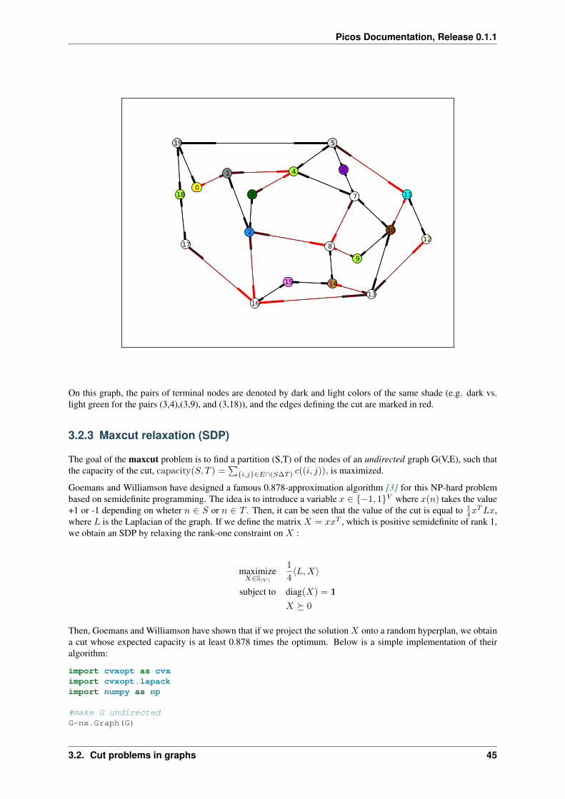
Picos Documentation, Release 0.1.1
0
1
2
3
4
5
6
7
8
9
10
11
12
13
1415
16
17
18
19
On this graph, the pairs of terminal nodes are denoted by dark and light colors of the same shade (e.g. dark vs.light green for the pairs (3,4),(3,9), and (3,18)), and the edges defining the cut are marked in red.
3.2.3 Maxcut relaxation (SDP)
The goal of the maxcut problem is to find a partition (S,T) of the nodes of an undirected graph G(V,E), such thatthe capacity of the cut, capacity(S, T ) =
∑{i,j}∈E∩(S∆T ) c((i, j)), is maximized.
Goemans and Williamson have designed a famous 0.878-approximation algorithm [3] for this NP-hard problembased on semidefinite programming. The idea is to introduce a variable x ∈ {−1, 1}V where x(n) takes the value+1 or -1 depending on wheter n ∈ S or n ∈ T . Then, it can be seen that the value of the cut is equal to 1
4xTLx,
where L is the Laplacian of the graph. If we define the matrix X = xxT , which is positive semidefinite of rank 1,we obtain an SDP by relaxing the rank-one constraint on X :
maximizeX∈S|V |
1
4〈L,X〉
subject to diag(X) = 1
X � 0
Then, Goemans and Williamson have shown that if we project the solution X onto a random hyperplan, we obtaina cut whose expected capacity is at least 0.878 times the optimum. Below is a simple implementation of theiralgorithm:
import cvxopt as cvximport cvxopt.lapackimport numpy as np
#make G undirectedG=nx.Graph(G)
3.2. Cut problems in graphs 45

Picos Documentation, Release 0.1.1
#allocate weights to the edgesfor (i,j) in G.edges():
G[i][j][’weight’]=c[i,j]+c[j,i]
maxcut = pic.Problem()X=maxcut.add_variable(’X’,(N,N),’symmetric’)
#Laplacian of the graphL=pic.new_param(’L’,1/4.*nx.laplacian(G))
#ones on the diagonalmaxcut.add_constraint(pic.tools.diag_vect(X)==1)#X positive semidefinitemaxcut.add_constraint(X>>0)
#objectivemaxcut.set_objective(’max’,L|X)
print maxcutmaxcut.solve(verbose = 0)
print ’bound from the SDP relaxation: {0}’.format(maxcut.obj_value())
#---------------------------##RANDOM PROJECTION ALGORITHM##---------------------------#
#Cholesky factorizationV=X.value
cvxopt.lapack.potrf(V)for i in range(N):
for j in range(i+1,N):V[i,j]=0
#random projection algorithm#Repeat 100 times or until we are within a factor .878 of the SDP optimal valuecount=0obj_sdp=maxcut.obj_value()obj=0while (count <100 or obj<.878*obj_sdp):
r=cvx.normal(20,1)x=cvx.matrix(np.sign(V*r))o=(x.T*L*x).value[0]if o>obj:
x_cut=xobj=o
count+=1
print ’value of the cut: {0}’.format(obj)S1=[n for n in range(N) if x[n]<0]S2=[n for n in range(N) if x[n]>0]cut = [(i,j) for (i,j) in G.edges() if x[i]*x[j]<0]
#we comment this because the output in unpredicatable for doctest:#print ’partition of the nodes:’#print ’S1: {0}’.format(S1)#print ’S2: {0}’.format(S2)
Generated output:
46 Chapter 3. Examples

Picos Documentation, Release 0.1.1
---------------------optimization problem (SDP):210 variables, 20 affine constraints, 210 vars in 1 SD cones
X : (20, 20), symmetric
maximize ⟨ L | X ⟩such thatdiag(X) = |1|X � |0|---------------------bound from the SDP relaxation: 478.2074...value of the cut: 471.0
Let us now draw this cut:
#display the cutimport pylab
fig=pylab.figure(figsize=(11,8))
pos=nx.spring_layout(G)
node_colors=[(’g’ if n in S1 else ’b’) for n in range(N)]
nx.draw_networkx(G,pos,edgelist=[e for e in G.edges() if e not in cut],node_color=node_colors)
nx.draw_networkx_edges(G,pos,edgelist=cut,edge_color=’r’)
#hide axisfig.gca().axes.get_xaxis().set_ticks([])fig.gca().axes.get_yaxis().set_ticks([])
pylab.show()
3.2. Cut problems in graphs 47

Picos Documentation, Release 0.1.1
0
1
2
3
4
5
6
7
8
9
10
11
12
13
1415
16
17
18
19
On this graph, the red edges are those defining the cut, and the nodes are blue or green depending on the partitionthey belong to.
3.2.4 References
1. “Maximal Flow through a Network”, LR Ford Jr and DR Fulkerson, Canadian journal of mathematics,1956.
2. “Analysis of LP relaxations for multiway and multicut problems”, D.Bertsimas, C.P. Teo and R. Vohra,Networks, 34(2), p. 102-114, 1999.
3. “Improved approximation algorithms for maximum cut and satisfiability problems using semidefinite pro-gramming”, M.X. Goemans and D.P. Williamson, Journal of the ACM, 42(6), p. 1115-1145, 1995.
48 Chapter 3. Examples
CHAPTER
FOUR
THE PICOS API
4.1 Problem
class picos.Problem(**options)This class represents an optimization problem. The constructor creates an empty problem. Some op-tions can be provided under the form key = value. See the list of available options in the doc ofset_all_options_to_default()
add_constraint(cons, key=None, ret=False)Adds a constraint in the problem.
Parameters
• cons (Constraint) – The constraint to be added.
• key (str.) – Optional parameter to describe the constraint with a key string.
• ret (bool.) – Do you want the added constraint to be returned ? This can be useful toaccess the dual of this constraint.
add_list_of_constraints(lst, it=None, indices=None, key=None, ret=False)adds a list of constraints in the problem. This fonction can be used with python list comprehensions(see the example below).
Parameters
• lst – list of Constraint.
• it (None or str or list.) – Description of the letters which should be used to replacethe dummy indices. The function tries to find a template for the string representationsof the constraints in the list. If several indices change in the list, their letters shouldbe given as a list of strings, in their order of appearance in the resulting string. Forexample, if three indices change in the constraints, and you want them to be named’i’, ’j’ and ’k’, set it = [’i’,’j’,’k’]. You can also group two indiceswhich always appear together, e.g. if ’i’ always appear next to ’j’ you could set it= [(’ij’,2),’k’]. Here, the number 2 indicates that ’ij’ replaces 2 indices.If it is set to None, or if the function is not able to find a template, the string of thefirst constraint will be used for the string representation of the list of constraints.
• indices (str.) – a string to denote the set where the indices belong to.
• key (str.) – Optional parameter to describe the list of constraints with a key string.
• ret (bool.) – Do you want the added list of constraints to be returned ? This can beuseful to access the duals of these constraints.
Example:
>>> import picos as pic>>> import cvxopt as cvx>>> prob=pic.Problem()
49
Picos Documentation, Release 0.1.1
>>> x=[prob.add_variable(’x[{0}]’.format(i),2) for i in range(5)]>>> x[# variable x[0]:(2 x 1),continuous #,# variable x[1]:(2 x 1),continuous #,# variable x[2]:(2 x 1),continuous #,# variable x[3]:(2 x 1),continuous #,# variable x[4]:(2 x 1),continuous #]
>>> y=prob.add_variable(’y’,5)>>> IJ=[(1,2),(2,0),(4,2)]>>> w={}>>> for ij in IJ:... w[ij]=prob.add_variable(’w[{0}]’.format(ij),3)...>>> u=pic.new_param(’u’,cvx.matrix([2,5]))>>> prob.add_list_of_constraints(... [u.T*x[i]<y[i] for i in range(5)],... ’i’,... ’[5]’)>>>>>> prob.add_list_of_constraints(... [abs(w[i,j])<y[j] for (i,j) in IJ],... [(’ij’,2)],... ’IJ’)>>>>>> prob.add_list_of_constraints(... [y[t] > y[t+1] for t in range(4)],... ’t’,... ’[4]’)>>>>>> print prob---------------------optimization problem (SOCP):24 variables, 9 affine constraints, 12 vars in 3 SO cones
x : list of 5 variables, (2, 1), continuousw : dict of 3 variables, (3, 1), continuousy : (5, 1), continuous
find varssuch thatu.T*x[i] < y[i] for all i in [5]||w[ij]|| < y[ij__1] for all ij in IJy[t] > y[t+1] for all t in [4]
---------------------
add_variable(name, size=1, vtype=’continuous’)adds a variable in the problem, and returns the corresponding instance of the Variable.
For example,
>>> prob=pic.Problem()>>> x=prob.add_variable(’x’,3)>>> x# variable x:(3 x 1),continuous #
Parameters
• name (str.) – The name of the variable.
• size (int or tuple.) – The size of the variable.
Can be either:
– an int n , in which case the variable is a vector of dimension n
50 Chapter 4. The PICOS API
Picos Documentation, Release 0.1.1
– or a tuple (n,m), and the variable is a n x m-matrix.
• vtype (str.) – variable type. Can be:
– ’continuous’ (default),
– ’binary’: 0/1 variable
– ’integer’: integer valued variable
– ’symmetric’: symmetric matrix
– ’semicont’: 0 or continuous variable satisfying its bounds
– ’semiint’: 0 or integer variable satisfying its bounds
Returns An instance of the class Variable.
check_current_value_feasibility(tol=1e-05)returns True if the current value of the variabless is a feasible solution, up to the tolerance tol. Iftol is set to None, the option parameter options[’tol’] is used instead. The integer feasibilityis checked with a tolerance of 1e-3.
constraints = Nonelist of all constraints
copy()creates a copy of the problem.
countCons = Nonenumner of (multidimensional) constraints
countVar = Nonenumber of (multidimensional) variables
get_constraint(ind)returns a constraint of the problem.
Parameters ind (int or tuple.) – There are two ways to index a constraint.
• if ind is an int n, then the nth constraint (starting from 0) will be returned, where allthe constraints are counted in the order where they were passed to the problem.
• if ind is a tuple (k, i), then the ith constraint from the kth group of constraints is re-turned (starting from 0). By group of constraints, it is meant a single constraint or a listof constraints added together with the function add_list_of_constraints().
• if ind is a tuple of length 1 (k, ), then the list of constraints of the kth group isreturned.
Example:
>>> import picos as pic>>> import cvxopt as cvx>>> prob=pic.Problem()>>> x=[prob.add_variable(’x[{0}]’.format(i),2) for i in range(5)]>>> y=prob.add_variable(’y’,5)>>> prob.add_list_of_constraints(... [(1|x[i])<y[i] for i in range(5)],... ’i’,... ’[5]’)>>> prob.add_constraint(y>0)>>> print prob---------------------optimization problem (LP):15 variables, 10 affine constraints
x : list of 5 variables, (2, 1), continuousy : (5, 1), continuous
4.1. Problem 51

Picos Documentation, Release 0.1.1
find varssuch that
⟨ |1| | x[i] ⟩ < y[i] for all i in [5]y > |0|
--------------------->>> prob.get_constraint(1) #2d constraint (numbered from 0)# (1x1)-affine constraint: ⟨ |1| | x[1] ⟩ < y[1] #>>> prob.get_constraint((0,3)) #4th consraint from the 1st group# (1x1)-affine constraint: ⟨ |1| | x[3] ⟩ < y[3] #>>> prob.get_constraint((1,)) #unique constraint of the 2d ’group’# (5x1)-affine constraint: y > |0| #>>> prob.get_constraint((0,)) #list of constraints of the 1st group[# (1x1)-affine constraint: ⟨ |1| | x[0] ⟩ < y[0] #,# (1x1)-affine constraint: ⟨ |1| | x[1] ⟩ < y[1] #,# (1x1)-affine constraint: ⟨ |1| | x[2] ⟩ < y[2] #,# (1x1)-affine constraint: ⟨ |1| | x[3] ⟩ < y[3] #,# (1x1)-affine constraint: ⟨ |1| | x[4] ⟩ < y[4] #]
>>> prob.get_constraint(5) #6th constraint# (5x1)-affine constraint: y > |0| #
get_valued_variable(name)Returns the value of the variable (as an cvxopt matrix) with the given name. If name refers to alist (resp. dict) of variables, named with the template name[index] (resp. name[key]), then thefunction returns the list (resp. dict) of these variables.
Parameters name (str.) – name of the variable, or of a list/dict of variables.
Warning: If the problem has not been solved, or if the variable is not valued, this function willraise an Exception.
get_variable(name)Returns the variable (as a Variable) with the given name. If name refers to a list (resp. dict) ofvariables, named with the template name[index] (resp. name[key]), then the function returnsthe list (resp. dict) of these variables.
Parameters name (str.) – name of the variable, or of a list/dict of variables.
is_continuous()Returns True if there are only continuous variables
numberAffConstraints = Nonetotal number of (scalar) affine constraints
numberConeConstraints = Nonenumber of SOC constraints
numberConeVars = Nonenumber of auxilary variables required to handle the SOC constraints
numberLSEConstraints = Nonenumber of LogSumExp constraints (+1 if the objective is a LogSumExp)
numberLSEVars = Nonenumber of vars in LogSumExp expressions
numberOfVars = Nonetotal number of (scalar) variables
numberQuadConstraints = Nonenumber of quadratic constraints (+1 if the objective is quadratic)
numberQuadNNZ = Nonenumber of nonzero entries in the matrices defining the quadratic expressions
52 Chapter 4. The PICOS API

Picos Documentation, Release 0.1.1
numberSDPConstraints = Nonenumber of SDP constraints
numberSDPVars = Nonesize of the s-vecotrized matrices involved in SDP constraints
obj_value()If the problem was already solved, returns the objective value. Otherwise, it raises anAttributeError.
remove_all_constraints()Removes all constraints from the problem
remove_constraint(ind)Deletes a constraint or a list of constraints of the problem.
Parameters ind (int or tuple.) – The indexing of constraints works as in the functionget_constraint():
• if ind is an integer n, the nth constraint (numbered from 0) is deleted
• if ind is a tuple (k, i), then the ith constraint from the kth group of con-straints is deleted (starting from 0). By group of constraints, it is meanta single constraint or a list of constraints added together with the functionadd_list_of_constraints().
• if ind is a tuple of length 1 (k, ), then the whole kth group of constraints is deleted.
Example:
>>> import picos as pic>>> import cvxopt as cvx>>> prob=pic.Problem()>>> x=[prob.add_variable(’x[{0}]’.format(i),2) for i in range(4)]>>> y=prob.add_variable(’y’,4)>>> prob.add_list_of_constraints(... [(1|x[i])<y[i] for i in range(4)], ’i’, ’[5]’)>>> prob.add_constraint(y>0)>>> prob.add_list_of_constraints(... [x[i]<2 for i in range(3)], ’i’, ’[3]’)>>> prob.add_constraint(x[3]<1)>>> prob.constraints[# (1x1)-affine constraint: ⟨ |1| | x[0] ⟩ < y[0] #,# (1x1)-affine constraint: ⟨ |1| | x[1] ⟩ < y[1] #,# (1x1)-affine constraint: ⟨ |1| | x[2] ⟩ < y[2] #,# (1x1)-affine constraint: ⟨ |1| | x[3] ⟩ < y[3] #,# (4x1)-affine constraint: y > |0| #,# (2x1)-affine constraint: x[0] < |2.0| #,# (2x1)-affine constraint: x[1] < |2.0| #,# (2x1)-affine constraint: x[2] < |2.0| #,# (2x1)-affine constraint: x[3] < |1| #]
>>> prob.remove_constraint(1) #2d constraint (numbered from 0) deleted>>> prob.constraints[# (1x1)-affine constraint: ⟨ |1| | x[0] ⟩ < y[0] #,# (1x1)-affine constraint: ⟨ |1| | x[2] ⟩ < y[2] #,# (1x1)-affine constraint: ⟨ |1| | x[3] ⟩ < y[3] #,# (4x1)-affine constraint: y > |0| #,# (2x1)-affine constraint: x[0] < |2.0| #,# (2x1)-affine constraint: x[1] < |2.0| #,# (2x1)-affine constraint: x[2] < |2.0| #,# (2x1)-affine constraint: x[3] < |1| #]
>>> prob.remove_constraint((1,)) #2d ’group’ of constraint deleted,... #i.e. the single constraint y>|0|>>> prob.constraints[# (1x1)-affine constraint: ⟨ |1| | x[0] ⟩ < y[0] #,# (1x1)-affine constraint: ⟨ |1| | x[2] ⟩ < y[2] #,
4.1. Problem 53

Picos Documentation, Release 0.1.1
# (1x1)-affine constraint: ⟨ |1| | x[3] ⟩ < y[3] #,# (2x1)-affine constraint: x[0] < |2.0| #,# (2x1)-affine constraint: x[1] < |2.0| #,# (2x1)-affine constraint: x[2] < |2.0| #,# (2x1)-affine constraint: x[3] < |1| #]
>>> prob.remove_constraint((2,)) #3d ’group’ of constraint deleted,... #(originally the 4th group, i.e. x[3]<|1|)>>> prob.constraints[# (1x1)-affine constraint: ⟨ |1| | x[0] ⟩ < y[0] #,# (1x1)-affine constraint: ⟨ |1| | x[2] ⟩ < y[2] #,# (1x1)-affine constraint: ⟨ |1| | x[3] ⟩ < y[3] #,# (2x1)-affine constraint: x[0] < |2.0| #,# (2x1)-affine constraint: x[1] < |2.0| #,# (2x1)-affine constraint: x[2] < |2.0| #]
>>> prob.remove_constraint((1,1)) #2d constraint of the 2d group (originally... #the 3rd group, i.e. x[1]<|2| )>>> prob.constraints[# (1x1)-affine constraint: ⟨ |1| | x[0] ⟩ < y[0] #,# (1x1)-affine constraint: ⟨ |1| | x[2] ⟩ < y[2] #,# (1x1)-affine constraint: ⟨ |1| | x[3] ⟩ < y[3] #,# (2x1)-affine constraint: x[0] < |2.0| #,# (2x1)-affine constraint: x[2] < |2.0| #]
remove_variable(name)Removes the variable name from the problem. :param name: name of the variable to remove. :typename: str.
set_all_options_to_default()set all the options to their default. The following options are available:
•General options common to all solvers:
–verbose = 1 : verbosity level [0(quiet)|1|2(loud)]
–solver = None : currently the available solvers are ’cvxopt’, ’cplex’, ’mosek’,’gurobi’, ’smcp’, ’zibopt’. The default None means that you let picos select asuitable solver for you.
–tol = 1e-8 : Relative gap termination tolerance for interior-point optimizers (feasibilityand complementary slackness).
–maxit = None : maximum number of iterations (for simplex or interior-point optimizers).This option is currently ignored by zibopt.
–lp_root_method = None : algorithm used to solve continuous LP problems, includingthe root relaxation of mixed integer problems. The default None selects automatically analgorithm. If set to psimplex (resp. dsimplex, interior), the solver will use a primalsimplex (resp. dual simplex, interior-point) algorithm. This option currently works only withcplex, mosek and gurobi.
–lp_node_method = None : algorithm used to solve subproblems at nodes of the branch-ing trees of mixed integer programs. The default None selects automatically an algorithm.If set to psimplex (resp. dsimplex, interior), the solver will use a primal simplex(resp. dual simplex, interior-point) algorithm. This option currently works only with cplex,mosek and gurobi.
–timelimit = None : time limit for the solver, in seconds. The default None means notime limit. This option is currently ignored by cvxopt and smcp.
–treememory = None : size of the buffer for the branch and bound tree, in Megabytes.This option currently works only with cplex.
–gaplim = 1e-4 : For mixed integer problems, the solver returns a solution as soon as thisvalue for the gap is reached (relative gap between the primal and the dual bound).
54 Chapter 4. The PICOS API

Picos Documentation, Release 0.1.1
–onlyChangeObjective = False : set this option to True if you have already solvedthe problem, and want to recompute the solution with a different objective funtion or differentparameter settings. This way, the constraints of the problem will not be parsed by picos nexttime solve() is called (this can lead to a huge gain of time).
–noprimals = False : if True, do not copy the optimal variable values in the valueattribute of the problem variables.
–noduals = False : if True, do not try to retrieve the dual variables.
–nbsol = None : maximum number of feasible solution nodes visited when solving amixed integer problem.
–hotstart = False [if True, the MIP optimizer tries to start from the solution] speci-fied (even partly) in the value attribute of the problem variables. This option currentlyworks only with cplex, mosek and gurobi.
–convert_quad_to_socp_if_needed = True : Do we convert the convex quadrat-ics to second order cone constraints when the solver does not handle them directly ?
•Specific options available for cvxopt/smcp:
–feastol = None : feasibility tolerance passed to cvx.solvers.options If feastol hasthe default value None, then the value of the option tol is used.
–abstol = None : absolute tolerance passed to cvx.solvers.options If abstol has thedefault value None, then the value of the option tol is used.
–reltol = None : relative tolerance passed to cvx.solvers.options If reltol has the de-fault value None, then the value of the option tol, multiplied by 10, is used.
•Specific options available for cplex:
–cplex_params = {} : a dictionary of cplex parameters to be set before the cplex opti-mizer is called. For example, cplex_params={’mip.limits.cutpasses’ : 5}will limit the number of cutting plane passes when solving the root node to 5.
–acceptable_gap_at_timelimit = None : If the the time limit is reached, the op-timization process is aborted only if the current gap is less than this value. The default valueNone means that we interrupt the computation regardless of the achieved gap.
•Specific options available for mosek:
–mosek_params = {} : a dictionary of mosek parameters to be set before the mosekoptimizer is called. For example, mosek_params={’simplex_abs_tol_piv’ :1e-4} sets the absolute pivot tolerance of the simplex optimizer to 1e-4.
•Specific options available for gurobi:
–gurobi_params = {} : a dictionary of gurobi parameters to be set before the gurobioptimizer is called. For example, gurobi_params={’NodeLimit’ : 25} limits thenumber of nodes visited by the MIP optimizer to 25.
set_objective(typ, expr)Defines the objective function of the problem.
Parameters
• typ (str.) – can be either ’max’ (maximization problem), ’min’ (minimizationproblem), or ’find’ (feasibility problem).
• expr – an Expression. The expression to be minimized or maximized. This pa-rameter will be ignored if typ==’find’.
set_option(key, val)Sets the option key to the value val.
Parameters
4.1. Problem 55
Picos Documentation, Release 0.1.1
• key (str.) – The key of an option (see the list of keys in the doc ofset_all_options_to_default()).
• val – New value for the option.
set_var_value(name, value, optimalvar=False)Sets the value attribute of the given variable.
Parameters
• name (str.) – name of the variable to which the value will be given
• value – The value to be given. The type of value must be recognized by the func-tion _retrieve_matrix(), so that it can be parsed into a cvxopt sparsematrix of the desired size.
Example
>>> prob=pic.Problem()>>> x=prob.add_variable(’x’,2)>>> prob.set_var_value(’x’,[3,4]) #this is equivalent to x.value=[3,4]>>> abs(x)**2#quadratic expression: ||x||**2 #>>> print (abs(x)**2)25.0
solve(**options)Solves the problem.
Once the problem has been solved, the optimal variables can be obtained thanks to the property valueof the class Expression. The optimal dual variables can be accessed by the property dual of theclass Constraint.
Parameters options – A list of options to update before the call to the solver. In particular,the solver can be specified here, under the form key = value. See the list of availableoptions in the doc of set_all_options_to_default()
Returns A dictionary sol which contains the information returned by the solver.
solver_selection()Selects an appropriate solver for this problem and sets the option ’solver’.
status = Nonestatus returned by the solver. The default when a new problem is created is ‘unsolved’.
typeType of Optimization Problem (‘LP’, ‘MIP’, ‘SOCP’, ‘QCQP’,...)
update_options(**options)update the option dictionary, for each pair of the form key = value. For a list of available optionsand their default values, see the doc of set_all_options_to_default().
variables = Nonedictionary of variables indexed by variable names
write_to_file(filename, writer=’picos’)This function writes the problem to a file.
Parameters
• filename (str.) – The name of the file where the problem will be saved. The extensionof the file (if provided) indicates the format of the export:
– ’.lp’: LP format . This format handles only linear constraints, unless the writer’cplex’ is used, and the file is saved in the extended cplex LP format
– ’.mps’: MPS format (recquires mosek, gurobi or cplex).
– ’.opf’: OPF format (recquires mosek).
56 Chapter 4. The PICOS API

Picos Documentation, Release 0.1.1
– ’.dat-s’: sparse SDPA format This format is suitable to save semidefinite pro-grams (SDP). SOC constraints are stored as semidefinite constraints with an arrowpattern.
• writer (str.) – The default writer is picos, which has its own LP and sparse SDPAwrite functions. If cplex, mosek or gurobi is installed, the user can pass the optionwriter=’cplex’, writer=’gurobi’ or writer=’mosek’, and the writefunction of this solver will be used.
4.2 picos.tools
picos.tools.available_solvers()Lists all available solvers
picos.tools.diag(exp, dim=1)if exp is an affine expression of size (n,m), diag(exp,dim) returns a diagonal matrix of size dim*n*m× dim*n*m, with dim copies of the vectorized expression exp[:] on the diagonal.
In particular:
•when exp is scalar, diag(exp,n) returns a diagonal matrix of size n×n, with all diagonal elementsequal to exp.
•when exp is a vector of size n, diag(exp) returns the diagonal matrix of size n×n with the vectorexp on the diagonal
Example
>>> import picos as pic>>> prob=pic.Problem()>>> x=prob.add_variable(’x’,1)>>> y=prob.add_variable(’y’,1)>>> pic.tools.diag(x-y,4)# (4 x 4)-affine expression: Diag(x -y) #>>> pic.tools.diag(x//y)# (2 x 2)-affine expression: Diag([x;y]) #
picos.tools.diag_vect(exp)Returns the vector with the diagonal elements of the matrix expression exp
Example
>>> import picos as pic>>> prob=pic.Problem()>>> X=prob.add_variable(’X’,(3,3))>>> pic.tools.diag_vect(X)# (3 x 1)-affine expression: diag(X) #
picos.tools.eval_dict(dict_of_variables)if dict_of_variables is a dictionary mapping variable names (strings) to variables, this functionreturns the dictionary names -> variable values.
picos.tools.lse(exp)shorter name for the constructor of the class LogSumExp
Example
>>> import picos as pic>>> import cvxopt as cvx>>> prob=pic.Problem()>>> x=prob.add_variable(’x’,3)>>> A=pic.new_param(’A’,cvx.matrix([[1,2],[3,4],[5,6]]))>>> pic.lse(A*x)<0# (2x1)-Geometric Programming constraint LSE[ A*x ] < 0 #
4.2. picos.tools 57
Picos Documentation, Release 0.1.1
picos.tools.new_param(name, value)Declare a parameter for the problem, that will be stored as a cvxopt sparse matrix. It is possible togive a list or a dictionary of parameters. The function returns a constant AffinExp (or a list or a dictof AffinExp) representing this parameter.
Note: Declaring parameters is optional, since the expression can as well be given by using normal variables.(see Example below). However, if you use this function to declare your parameters, the names of theparameters will be displayed when you print an Expression or a Constraint
Parameters
• name (str.) – The name given to this parameter.
• value – The value (resp list of values, dict of values) of the parameter. The type ofvalue (resp. the elements of the list value, the values of the dict value) should beunderstandable by the function _retrieve_matrix().
Returns A constant affine expression (AffinExp) (resp. a list of AffinExp of the samelength as value, a dict of AffinExp indexed by the keys of value)
Example:
>>> import cvxopt as cvx>>> prob=pic.Problem()>>> x=prob.add_variable(’x’,3)>>> B={’foo’:17.4,’matrix’:cvx.matrix([[1,2],[3,4],[5,6]]),’ones’:’|1|(4,1)’}>>> B[’matrix’]*x+B[’foo’]# (2 x 1)-affine expression: [ 2 x 3 MAT ]*x + |17.4| #>>> #(in the string above, |17.4| represents the 2-dim vector [17.4,17.4])>>> B=pic.new_param(’B’,B)>>> #now that B is a param, we have a nicer display:>>> B[’matrix’]*x+B[’foo’]# (2 x 1)-affine expression: B[matrix]*x + |B[foo]| #
picos.tools.sum(lst, it=None, indices=None)sum of a list of affine expressions. This fonction can be used with python list comprehensions (see theexample below).
Parameters
• lst – list of AffinExp.
• it (None or str or list.) – Description of the letters which should be used to replacethe dummy indices. The function tries to find a template for the string representationsof the affine expressions in the list. If several indices change in the list, their lettersshould be given as a list of strings, in their order of appearance in the resulting string.For example, if three indices change in the summands, and you want them to be named’i’, ’j’ and ’k’, set it = [’i’,’j’,’k’]. You can also group two indiceswhich always appear together, e.g. if ’i’ always appear next to ’j’ you could set it= [(’ij’,2),’k’]. Here, the number 2 indicates that ’ij’ replaces 2 indices. Ifit is set to None, or if the function is not able to find a template, the string of the firstsummand will be used for the string representation of the sum.
• indices (str.) – a string to denote the set where the indices belong to.
Example:
>>> import picos as pic>>> prob=pic.Problem()>>> x={}>>> names=[’foo’,’bar’,’baz’]>>> for n in names:... x[n]=prob.add_variable( ’x[{0}]’.format(n),(3,5) )
58 Chapter 4. The PICOS API

Picos Documentation, Release 0.1.1
>>> x{’baz’: # variable x[baz]:(3 x 5),continuous #,’foo’: # variable x[foo]:(3 x 5),continuous #,’bar’: # variable x[bar]:(3 x 5),continuous #}>>> pic.sum([x[n] for n in names],’n’,’names’)# (3 x 5)-affine expression: Σ_{n in names} x[n] #>>> pic.sum([(i+1) * x[n] for i,n in enumerate(names)],[’i’,’n’],’[3] x names’) #two indices# (3 x 5)-affine expression: Σ_{i,n in [3] x names} i*x[n] #>>> IJ = [(1,2),(2,4),(0,1),(1,3)]>>> pic.sum([x[’foo’][ij] for ij in IJ],[(’ij’,2)],’IJ’) #double index# (1 x 1)-affine expression: Σ_{ij in IJ} x[foo][ij] #
picos.tools._retrieve_matrix(mat, exSize=None)parses the variable mat and convert it to a cvxopt sparse matrix. If the variable exSize is provided,the function tries to return a matrix that matches this expected size, or raise an error.
Warning: If there is a conflit between the size of mat and the expected size exsize, the function mightstill return something without raising an error !
Parameters mat – The value to be converted into a cvx.spmatrix. The function will try to parsethis variable and format it to a vector/matrix. mat can be of one of the following types:
• list [creates a vecor of dimension len(list)]
• cvxopt matrix
• cvxopt sparse matrix
• numpy array
• int or real [creates a vector/matrix of the size exSize (or of size (1,1) if exSize isNone), whith all entries equal to mat.
• following strings:
– ‘|a|‘ for a matrix with all terms equal to a
– ‘|a|(n,m)‘ for a matrix forced to be of size n x m, with all terms equal to a
– ‘e_i(n,m)‘ matrix of size (n,m), with a 1 on the ith coordinate (and 0 elsewhere)
– ‘e_i,j(n,m)‘ matrix of size (n,m), with a 1 on the (i,j)-entry (and 0 elsewhere)
– ‘I‘ for the identity matrix
– ‘I(n)‘ for the identity matrix, forced to be of size n x n.
– ‘a%s‘, where %s is one of the above string: the matrix that should be returned whenmat == %s, multiplied by the scalar a.
Returns A tuple of the form (M, s), where M is the conversion of mat into a cvxopt sparsematrix, and s is a string representation of mat
Example:
>>> import picos as pic>>> pic.tools._retrieve_matrix([1,2,3])(<3x1 sparse matrix, tc=’d’, nnz=3>, ’[ 3 x 1 MAT ]’)>>> pic.tools._retrieve_matrix(’e_5(7,1)’)(<7x1 sparse matrix, tc=’d’, nnz=1>, ’e_5’)>>> print pic.tools._retrieve_matrix(’e_11(7,2)’)[0][ 0 0 ][ 0 0 ][ 0 0 ][ 0 0 ][ 0 1.00e+00][ 0 0 ][ 0 0 ]
4.2. picos.tools 59
Picos Documentation, Release 0.1.1
>>> print pic.tools._retrieve_matrix(’5.3I’,(2,2))(<2x2 sparse matrix, tc=’d’, nnz=2>, ’5.3I’)
4.3 Expression
class picos.Expression(string)The parent class of AffinExp (which is the parent class of Variable), Norm, LogSumExp, andQuadExp.
4.3.1 AffinExp
class picos.AffinExp(factors=None, constant=None, size=(1, 1), string=‘0’)A class for defining vectorial (or matrix) affine expressions. It derives from Expression.
Overloaded operators
+ sum (with an affine or quadratic expression)
+= in-place sum (with an affine or quadratic expression)
- substraction (with an affine or quadratic expression) or unitary minus
* multiplication (by another affine expression or a scalar)
/ division (by a scalar)
| scalar product (with another affine expression)
[.] slice of an affine expression
abs() Euclidean norm (Frobenius norm for matrices)
** exponentiation (works with arbitrary powers for constant affine expressions, andonly with the exponent 2 if the affine expression involves some variables)
& horizontal concatenation (with another affine expression)
// vertical concatenation (with another affine expression)
< less or equal (than an affine or quadratic expression)
> greater or equal (than an affine or quadratic expression)
== is equal (to another affine expression)
<< less than inequality in the Loewner ordering (linear matrix inequality �)
>> greater than inequality in the Loewner ordering (linear matrix inequality �)
Warning: We recall here the implicit assumptions that are made when using relation operator overloads,in the following two situations:
•the rotated second order cone constraint abs(exp1)**2 < exp2 * exp3 implicitely as-sumes that the scalar expression exp2 (and hence exp3) is nonnegative.
•the linear matrix inequality exp1 >> exp2 only tells picos that the symmetric matrix whoselower triangular elements are those of exp1-exp2 is positive semidefinite. The matrixexp1-exp2 is not constrained to be symmetric. Hence, you should manually add the con-straint exp1-exp2 == (exp1-exp2).T if it is not clear from the data that this matrix issymmetric.
TTransposition
constant = Noneconstant of the affine expression, stored as a cvxopt sparse matrix.
60 Chapter 4. The PICOS API

Picos Documentation, Release 0.1.1
factors = Nonedictionary storing the matrix of coefficients of the linear part of the affine expressions. The matricesof coefficients are always stored with respect to vectorized variables (for the case of matrix variables),and are indexed by instances of the class Variable.
is0()is the expression equal to 0 ?
isconstant()is the expression constant (no variable involved) ?
size = Nonesize of the affine expression
valuevalue of the affine expression
Variable
class picos.Variable(name, size, Id, startIndex, vtype=’continuous’)This class stores a variable. It derives from AffinExp.
Id = NoneAn integer index
endIndex = Noneend position in the global vector of all variables
name = NoneThe name of the variable (str)
startIndex = Nonestarting position in the global vector of all variables
valuevalue of the variable. The value of a variable is defined in the following two situations:
•The user has assigned a value to the variable, by using either the present value attribute, or thefunction set_var_value() of the class Problem.
•The problem involving the variable has been solved, and the value attribute stores the optimalvalue of this variable.
vtype = Noneone of the following strings:
•‘continuous’ (continuous variable)
•‘binary’ (binary 0/1 variable)
•‘integer’ (integer variable)
•‘symmetric’ (symmetric matrix variable)
•‘semicont’ (semicontinuous variable [can take the value 0 or any other admissible value])
•‘semiint’ (semi integer variable [can take the value 0 or any other integer admissible value])
4.3.2 Norm
class picos.Norm(exp)Euclidean (or Frobenius) norm of an Affine Expression. This class derives from Expression.
Overloaded operators
** exponentiation (only implemented when the exponent is 2)
4.3. Expression 61
Picos Documentation, Release 0.1.1
< less or equal (than a scalar affine expression)
exp = NoneThe affine expression of which we take the norm
4.3.3 QuadExp
class picos.QuadExp(quad, aff, string, LR=None)Quadratic expression. This class derives from Expression.
Overloaded operators
+ addition (with an affine or a quadratic expression)
- substraction (with an affine or a quadratic expression) or unitary minus
* multiplication (by a scalar or a constant affine expression)
< less or equal than (another quadratic or affine expression).
> greater or equal than (another quadratic or affine expression).
LR = Nonestores a factorization of the quadratic expression, if the expression was entered in a factorized form.We have:
•LR=None when no factorization is known
•LR=(aff,None) when the expression is equal to ||aff||**2
•LR=(aff1,aff2) when the expression is equal to aff1*aff2.
aff = Noneaffine expression representing the affine part of the quadratic expression
quad = Nonedictionary of quadratic forms, stored as matrices representing bilinear forms with respect to two vec-torized variables, and indexed by tuples of instances of the class Variable.
4.3.4 LogSumExp
class picos.LogSumExp(exp)
Log-Sum-Exp applied to an affine expression. If the affine expression z is of size N , with elementsz1, z2, . . . , zN , then LogSumExp(z) represents the expression log(
∑ni=1 e
zi). This class derives fromExpression.
Overloaded operator
< less or equal than (the rhs must be 0, for geometrical programming)
valuevalue of the logsumexp expression
4.4 Constraint
class picos.Constraint(typeOfConstraint, Id, Exp1, Exp2, Exp3=None, dualVariable=None,key=None)
A class for describing a constraint.
Exp1 = NoneLHS
62 Chapter 4. The PICOS API
Picos Documentation, Release 0.1.1
Exp2 = NoneRHS (ignored for constraints of type lse and quad, where Exp2 is set to 0)
Exp3 = NoneSecond factor of the RHS for RScone constraints (see typeOfConstraint).
Id = NoneAn integer identifier
dualValue of the dual variable associated to this constraint
See the note on dual variables in the tutorial for more information.
key = NoneA string to give a key name to the constraint
slackValue of the slack variable associated to this constraint (should be nonnegative/zero if the inequal-ity/equality is satisfied)
slack_var()returns the slack of the constraint (For an inequality of the type lhs<rhs, the slack is rhs-lhs, andfor lhs>rhs the slack is lhs-rhs).
typeOfConstraint = NoneA string from the following values, indicating the type of constraint:
•lin<, lin= or lin> : Linear (in)equality Exp1 ≤ Exp2, Exp1 = Exp2 or Exp1 ≥Exp2.
•SOcone : Second Order Cone constraint ||Exp1|| < Exp2.
•RScone : Rotated Cone constraint ||Exp1||**2 < Exp2 * Exp3.
•lse : Geometric Programming constraint LogSumExp(Exp1)<0
•quad: scalar quadratic constraint Exp1 < 0.
•sdp< or sdp>: semidefinite constraint Exp1 � Exp2 or Exp1 � Exp2.
4.4. Constraint 63

Picos Documentation, Release 0.1.1
64 Chapter 4. The PICOS API

INDEX
_retrieve_matrix() (in module picos.tools), 59
add_constraint() (picos.Problem method), 49add_list_of_constraints() (picos.Problem method), 49add_variable() (picos.Problem method), 50aff (picos.QuadExp attribute), 62AffinExp (class in picos), 60available_solvers() (in module picos.tools), 57
check_current_value_feasibility()(picos.Problem method), 51
constant (picos.AffinExp attribute), 60Constraint (class in picos), 62constraints (picos.Problem attribute), 51copy() (picos.Problem method), 51countCons (picos.Problem attribute), 51countVar (picos.Problem attribute), 51
diag() (in module picos.tools), 57diag_vect() (in module picos.tools), 57dual (picos.Constraint attribute), 63
endIndex (picos.Variable attribute), 61eval_dict() (in module picos.tools), 57exp (picos.Norm attribute), 62Exp1 (picos.Constraint attribute), 62Exp2 (picos.Constraint attribute), 62Exp3 (picos.Constraint attribute), 63Expression (class in picos), 60
factors (picos.AffinExp attribute), 61
get_constraint() (picos.Problem method), 51get_valued_variable() (picos.Problem method), 52get_variable() (picos.Problem method), 52
Id (picos.Constraint attribute), 63Id (picos.Variable attribute), 61is0() (picos.AffinExp method), 61is_continuous() (picos.Problem method), 52isconstant() (picos.AffinExp method), 61
key (picos.Constraint attribute), 63
LogSumExp (class in picos), 62LR (picos.QuadExp attribute), 62lse() (in module picos.tools), 57
name (picos.Variable attribute), 61new_param() (in module picos.tools), 57Norm (class in picos), 61numberAffConstraints (picos.Problem attribute), 52numberConeConstraints (picos.Problem attribute), 52numberConeVars (picos.Problem attribute), 52numberLSEConstraints (picos.Problem attribute), 52numberLSEVars (picos.Problem attribute), 52numberOfVars (picos.Problem attribute), 52numberQuadConstraints (picos.Problem attribute), 52numberQuadNNZ (picos.Problem attribute), 52numberSDPConstraints (picos.Problem attribute), 52numberSDPVars (picos.Problem attribute), 53
obj_value() (picos.Problem method), 53
picos.tools (module), 57Problem (class in picos), 49
quad (picos.QuadExp attribute), 62QuadExp (class in picos), 62
remove_all_constraints() (picos.Problem method), 53remove_constraint() (picos.Problem method), 53remove_variable() (picos.Problem method), 54
set_all_options_to_default() (picos.Problem method),54
set_objective() (picos.Problem method), 55set_option() (picos.Problem method), 55set_var_value() (picos.Problem method), 56size (picos.AffinExp attribute), 61slack (picos.Constraint attribute), 63slack_var() (picos.Constraint method), 63solve() (picos.Problem method), 56solver_selection() (picos.Problem method), 56startIndex (picos.Variable attribute), 61status (picos.Problem attribute), 56sum() (in module picos.tools), 58
T (picos.AffinExp attribute), 60type (picos.Problem attribute), 56typeOfConstraint (picos.Constraint attribute), 63
update_options() (picos.Problem method), 56
value (picos.AffinExp attribute), 61
65

Picos Documentation, Release 0.1.1
value (picos.LogSumExp attribute), 62value (picos.Variable attribute), 61Variable (class in picos), 61variables (picos.Problem attribute), 56vtype (picos.Variable attribute), 61
write_to_file() (picos.Problem method), 56
66 Index