Pi - CMS-SMC

Pi in the

SkyIssue 14, Fall 2010

In ThIs Issue:(-1) x (-1)=1 . . . but WHY?Palindrome DatesPrimes from FractionsReasoning from the Specific to the GeneralThe Mathematics of Climate Modelling

1

On the CoverPredicting the evolution of the Earth’s climate system is one of the most daunting mathematical modeling challenges that humanity has ever undertaken. In his article on page 17, Adam Monahan discusses the interweaving of mathematics with modern climate science.

Editorial BoardJohn Bowman (University of Alberta)Tel: (780) 492-0532, E-mail: [email protected] Bremner (University of Saskatchewan)Tel: (306) 966-6122, E-mail: [email protected] Campbell (Archbishop MacDonald High, Edmonton)Tel: (780) 441-6000, E-mail: [email protected] Diacu (University of Victoria)Tel: (250) 721-6330, E-mail: [email protected] Friesen (Galileo Educational Network, Calgary)Tel: (403) 220-8942, E-mail: [email protected] Hamilton (Masters Academy and College, Calgary)Tel: (403) 242-7034, E-mail: [email protected] Hoechsmann (University of British Columbia)Tel: (604) 822-3782, E-mail: [email protected] Hrimiuc (University of Alberta)Tel: (780) 492-3532, E-mail: [email protected] Lamoureux (University of Calgary)Tel: (403) 220-8214, E-mail: [email protected] Leeming (University of Victoria)Tel: (250) 472-4928, E-mail: [email protected] Mark MacLean (University of British Columbia)Tel: (604) 822-5552, E-mail: [email protected] Maidorn (University of Regina)Tel: (306) 585-4013, E-mail: [email protected] Swonnell (Greater Victoria School District)Tel: (250) 477-9706, E-mail: [email protected]

Managing EditorAnthony Quas (University of Victoria)Tel: (250) 721-7463, E-mail: [email protected]

Contact InformationPi in the SkyPIMS University of Victoria Site Office, SSM Building Room A418bPO Box 3060 STN CSC, 3800 Finnerty Road, Victoria, BC, V8W 3R4T/(250) 472-4271 F/(250) 721-8958 E-mail: [email protected]

Pi in the Sky is a publication of the Pacific Institute for the Mathematical Sciences (PIMS). PIMS is supported by the Natural Sciences and Engineering Research Council of Canada, the Province of Alberta, the Province of British Columbia, the Province of Saskatchewan, Simon Fraser University, the University of Alberta, the University of British Columbia, the University of Calgary, the University of Lethbridge, the University of Regina, the University of Victoria and the University of Washington.

Pi in the Sky is aimed primarily at high school students and teachers, with the main goal of providing a cultural context/landscape for mathematics. It has a natural extension to junior high school students and undergraduates, and articles may also put curriculum topics in a different perspective.

Submission InformationFor details on submitting articles for our next edition of Pi in the Sky, please see:

http://www.pims.math.ca/resources/publications/pi-sky

Table of Contents

Editorialby Anthony Quas . . . . . . . . . . . . . . . . . . . . . . . . . . . . . . . . . . . . 1

(-1) x (-1) = 1 . . . but WHY?by Marie Kim . . . . . . . . . . . . . . . . . . . . . . . . . . . . . . . . . . . . . . . 3

Palindrome Dates in Four-Digit Yearsby Aziz S. Inan . . . . . . . . . . . . . . . . . . . . . . . . . . . . . . . . . . . . . . 5

Primes from Fractionsby Alex P. Lamoureux and Michael P. Lamoureux. . . . . . . . . . . 8

Reasoning from the Specific to the Generalby Bill Russell . . . . . . . . . . . . . . . . . . . . . . . . . . . . . . . . . . . . . . 11

Book ReviewPythagorean CrimesReviewed by Gord Hamilton . . . . . . . . . . . . . . . . . . . . . . . . . . 15

The Mathematics of Climate Modellingby Adam H. Monahan. . . . . . . . . . . . . . . . . . . . . . . . . . . . . . . . 17

Pi in the Sky Math ChallengesSolutions to problems published in Issue 13. . . . . . . . . . . . . . . 22New Problems . . . . . . . . . . . . . . . . . . . . . . . . . . . . . . . . . . . . . 25

1

EditorialAnthony Quas

MATHEMATICAL ModELLIng: WHAT, HoW And WHY?

In my work and outside it too I often hear about Mathematical Modelling. In this editorial I'll say a bit about what it is; how to do it; and why it's important.

What is Mathematical Modelling?

First let's try a quick answer: Mathematical Modelling is the process of using mathematics to understand something `in the real world'. For high school students the closest thing to this in the curriculum might be the (often-dreaded) word problems. Here is an example taken from the internet:

Mr.S is planting flowers to give his girl friend on Valentine's day, which is half a year away. Currently the flowers are 7 inches tall and will be fully grown once they reach one foot. If the flowers grow at a rate of half an inch per month, then how large will they be on the day? Will the flowers be fully grown? or will he have to find another gift?

The aim here is to take something which is on the surface not a mathematical question, translate it into a mathematical question, solve the mathematical question and translate the answer back into the framework of the original question.

In this case we let x denote the height of the flowers on Valentine's Day and say that x = 7 + t / 2 where t is the number of months until Valentine's Day. Since we're told it's half a year away we have t = 6 so that we can compute x = 10. Since we're told the flowers will be 12 inches when they're fully grown it sounds as though `Mr.S' will have to think of a new present.

For some more advanced examples, here are some other questions that might be approached using mathematical modelling.

When light is reflected in water the r e f l e c t i o n seems to be stretched out along the line connecting the viewer and the source. Why is this? Why isn't it stretched in the perpendicular d i r e c t i o n (horizontally in this picture)?

In the case of a fast-spreading epidemic involving an unknown disease (e.g. the SARS epidemic that hit China in late 2002 / early 2003 and spread to other countries including Canada) what are the best policies to follow to minimize sickness and death from the disease while avoiding over-reacting?

Finally one of the most important cases of all: climate modelling. Here you're trying to predict the weather patterns in 10 years; 20 years; 100 years. For more information on this see the article in this issue by Adam Monahan.

How do you do Mathematical Modelling?

Just as in the case of the word problem, a first step is trying to decide which variables to study in the problem. There is an important difference though. The word problem is typically constructed to give you all of the information you need to solve the problem (and no more). Generally the variables are given to you in the statement of the problem itself. When you're doing more advanced modelling you have to decide which variables to include (and often equally importantly which ones to leave out of consideration).

2 3

www.xkcd.com

This last idea is at first sight quite surprising. Surely the best model is the one that takes everything into account? Actually that's not usually considered to be the case. Rather a good model is usually considered to be the simplest one that explains the behaviour you're trying to study. This is an important idea that is sometimes called `Occam's Razor' (named after a 14th Century monk who first expressed it).

For example in the case of the reflected lights one might try to take account of the positions of all of the water molecules! This would probably be a bad idea because people don't know exactly how liquids work. Also because there are a number of trillion trillion water molecules in the picture it would be impossible to do any computations even if you did know where they all were.

In practice what you do is this: pick out some variables that you think could be important (in the water case I used the `slopiness' of the water: how far away from being flat it is as a variable for example) and try to write down some equations relating the observations to the situation you're modelling. This may involve making some guesses as to how things work. Test your model: does it give the results you expected?; can you apply it to make predictions in situations other than the one

where you know the answer? If it's not working you may need to tweak the model to improve it.

Why does mathematical modelling matter?

Mathematical modelling can be great or it can be useless. It all depends on the model chosen. Good mathematical modelling should make some predictions that you can test with existing data (it's important that you haven't already used the data to build the model-otherwise you end up with a circular argument: you build the model to work for a certain set of data and then check that it works with that same data). It should then make some predictions that you can test in the future.

You can use mathematical modelling to test ideas that would be impractical or unethical to do as an actual experiment. For instance in the SARS modelling example you might want to predict what would happen if we took no action and compare it to the effect of (say) shutting down schools and airports for two weeks. Doing an actual experiment would be politically impossible but doing it in the model doesn't impact people in the same way.

In the best case, mathematical modelling tells you how things work and informs decisions. It is an invaluable tool across science and economics.

2 3

Marie Kim is at Cheong Shim International Academy, currently in 11th grade. She's from South Korea, and plans to go to the U.S. for college and major in biology or neurology.

Negative numbers. Most students find the concept hard to understand and to accept at first. Mathematicians before Descartes refused to accept negative numbers, including the great Pascal himself. Negative numbers actually are believed to have been found in the East the earliest, in China. An ancient Chinese text, written in B.C. 1000, titled \Ku Jang San Sul" - meaning \nine arithmetic formulas"- includes in part a computation of negative numbers.

(-1) x (-1) = 1 . . . but WHY?Marie Kim, Cheong Shim International Academy

1. Pattern

2 x 2 = 4 1 x 2 = 2 0 x 2 = 0 (-1) x 2 = (-2) (-2) x 2 = (-4)

2 x 1 = 2 1 x 1 = 1 0 x 1 = 0 (-1) x 1 = (-1) (-2) x 1 = (-2)

2 x 0 = 0 1 x 0 = 0 0 x 0 = 0 (-1) x 0 = 0 (-2) x 0 = 0

Take a look at the pattern above. In each row, you'll be able to find that constant decrease in the number multiplied results in constant change in the product. The same for each column. Applying this same pattern, the next row will be:

2 x (-1) = (-2) 1 x (-1) = (-1) 0 x (-1) = 0 (-1) x (-1) = 1 (-2) x (-1) = 2

This pattern is an initial indication why the statement \negative number multiplied by negative number results in positive number" might be correct.

2. number line

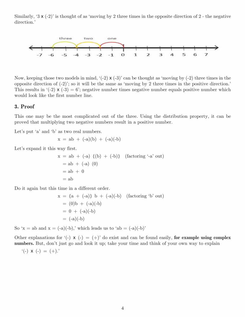
On the number line, `3 x 2' is thought of as `moving by 2 three times in the same direction as 2 - the positive direction.'

*2

2. Number line

On the number line, `2 x 3' is thought as `moving by 2 three times in the same direction as 2 - the positive direction.'

Similarly, `(-2) x 3' is thought as `moving by 2 three times in the opposite direction of 2 - the negative direction.'

Now, keeping those two models in mind, `(-2) x (-3)' can be thought as `moving by (-2) three times in the opposite direction of (-2)'; so it will be the same as `moving by 2 three times in the positive direction.' This results in `(-2) x (-3) = 6'; negative number times negative number equals positive number which would look like the first number line.

3. Proof

This one may be the most complicated out of the three. Using the distribution property, it can be proved that multiplying two negative numbers result in a positive number.

Let's put `a' and `b' as two real numbers.

x = ab + (-a)(b) + (-a)(-b)

Positive and negative numbers are often explained with the model of `debt and profit.' Profit is positive and debt is negative; adding positive numbers results in profit while adding negative numbers deducts profit - adding to debt. This model however, failed to make people understand the concept of multiplying a negative number by a negative number since it is hard to find such cases in everyday life.

How is the concept `negative number x negative number' explained, then? There are quite a few illustrations and models that are available to help people understand and accept such a concept. Out of those explanations, here are three easy ones.

4 5

Similarly, 3 x (-2)' is thought of as moving by 2 three times in the opposite direction of 2 - the negative direction.'

Now, keeping those two models in mind, (-2) x (-3)' can be thought as moving by (-2) three times in the opposite direction of (-2)'; so it will be the same as `moving by 2 three times in the positive direction.' This results in `(-2) x (-3) = 6'; negative number times negative number equals positive number which would look like the first number line.

3. Proof



x = ab + (-a)(b) + (-a)(-b)

Let's expand it this way first.

x = ab + (-a) {(b) + (-b)} (factoring `-a' out)

x = ab + (-a) (0)

x = ab + 0

x = ab

Do it again but this time in a different order.

x = {a + (-a)} b + (-a)(-b) (factoring `b' out)

x = (0)b + (-a)(-b)

x = 0 + (-a)(-b)

x = (-a)(-b)

So `x = ab and x = (-a)(-b),' which leads us to `ab = (-a)(-b)'

Other explanations for `(-) x (-) = (+)' do exist and can be found easily, for example using complex numbers. But, don't just go and look it up; take your time and think of your own way to explain

`(-) x (-) = (+).'

*2

2. Number line

On the number line, `2 x 3' is thought as `moving by 2 three times in the same direction as 2 - the positive direction.'

Similarly, `(-2) x 3' is thought as `moving by 2 three times in the opposite direction of 2 - the negative direction.'

Now, keeping those two models in mind, `(-2) x (-3)' can be thought as `moving by (-2) three times in the opposite direction of (-2)'; so it will be the same as `moving by 2 three times in the positive direction.' This results in `(-2) x (-3) = 6'; negative number times negative number equals positive number which would look like the first number line.

3. Proof



x = ab + (-a)(b) + (-a)(-b)

4 5

Aziz Inan was born in Turkey, did his PhD at Stanford and now teaches Electrical Engineering at University of Portland. He enjoys posing Recreational Math Puz-zles. He has noted that even his name has a puzzling geometric property. Write out AZIZ INAN. Swap A’s and I’s and rotate the consonants by 90 degrees. The two names switch places!

Introduction

In most of the world's countries, a specific calendar date in a four-digit year is expressed in the format DD/MM/YYYY (or DD.MM.YYYY or DD-MM-YYYY) where the first two digits (DD) are reserved for the day, the next two (MM) for the month and the last four (YYYY) for the year numbers. (The United States is one of the few countries which use the MM/DD/YYYY date format in which the places of the month and the day numbers are switched.) In general, if one removes the separators between the day, the month and the year numbers, a full date number consists of a single eight-digit number sequence given as DDMMYYYY. For example, the birth date of the famous American recreational mathematician Martin Gardner is 21 October 1914 which can be expressed as a single date number as 21101914 in the DDMMYYYY format (or 10211914 in the MMDDYYYY format).

Palindrome dates

Assuming each date in all the four-digit years is assigned a single eight-digit date n u m b e r DDMMYYYY, a question that comes to mind

is, \Can some of these eight-digit full dates be palindrome numbers?" (A palindrome number is a number that reads the same forwards or backwards [1-2].)

The answer is yes, and these special dates are called palindrome dates.

For example, in the DDMMYYYY date format, the first palindrome date of this (21st) century occurred on 10 February 2001 since this date, expressed as the single date number 10022001, is indeed a palindrome number. Note that palindrome date 10022001 is also the first palindrome date of this century that occurred in the MMDDYYYY date format, but it corresponds to a different actual date, which is October 2, 2001.

Generally speaking, palindrome dates are very rare and sometimes don't occur for centuries. If any, only a single palindrome date can exist in a given four-digit year Y1Y2Y3Y4. Also, among all four-digit years, a specific date designated by both month and day numbers as D1D2M1M2 (or M1M2D1D2) can be a palindrome date only once represented by a date number D1D2M1M2M2M1D2D1 (or M1M2D1D2D2D1M2M1).

In the DDMMY1Y2Y3Y4 date format, since each single palindrome date number must satisfy

Palindrome dates in Four-digit YearsAziz S. Inan

Table 1

Palindrome date combinations in the DDMMY1Y2Y3Y4 date format. Note that the total number of palindrome dates in each category adds up to 335.

D=Y4 D=Y3 M=Y2 M=Y1 Y1 Y2 Y3 Y4 N0 1 to 9 0 1 to 9 1 to 9 0 1 to 9 0 810 1 to 9 1 1,2 1,2 1 1 to 9 0 181,2 0 to 9 0 1 to 9 1 to 9 0 0 to 9 1,2 1801,2 0 to 9 1 1,2 1,2 1 0 to 9 1,2 403 0 0 1,3 to 9 1,3 to 9 0 0 3 83 1 0 1,3,5,7,8 1,3,5,7,8 0 1 3 53 0 1 1 1 1 0 3 13 1 1 0,2 0,2 1 1 3 2

6 7

*5

each single palindrome date number must satisfy Y4Y3Y2Y1Y1Y2Y3Y4, palindrome dates can only occur in years ending with a digit Y4 less than four (since day number cannot exceed 31). In addition, the hundredth digit Y2 of the year number of the palindrome date must either be zero or one (since month number cannot exceed 12). In the special case when the thousandth digit Y1 of the year satisfies Y1 > 2, Y2 must equal zero. In other words, palindrome dates in the second and third millenniums (years 1001 to 3000) can only occur in the first two centuries of each millennium. On the other hand, palindrome dates that fall between fourth and tenth millenniums (years 3001 to 10000) can only occur in the first century of each millennium. Also, between years 1000 to 10000, palindrome dates in each century all fall on the same month with month number Y2Y1. Table 1 provides allpossible combinationsof palindrome dates in the DDMMY1Y2Y3Y4 date format categorized in terms of different values and ranges of digits Y4, Y2, Y3 and Y1, where N is the total number of palindrome dates in each category. Based on Table 1, in the DDMMYYYY date format, a total of 335 palindrome dates exist among all the four-digit years.

In the MMDDY1Y2Y3Y4 date format, palindrome dates represented by Y4Y3Y2Y1Y1Y2Y3Y4 can only occur in years ending with digit Y4 equal to either zero or one since the month number cannot exceed 12. In the case when Y4 = 1, the tenth digit Y3 of the year number cannot exceed two. In addition, the second digit Y2 of the year number of the palindrome date must be less than four since the day number cannot exceed 31. Furthermore, if Y1 > 1, then, Y2 < 3. That is, for the MMDDY1Y2Y3Y4 date format, palindrome dates in the second millennium (years 1001 to 2000) can occur only in the first four centuries of each millennium. On the other

hand, palindrome dates between the third and tenth millenniums (2001 to 10000) only occur in the first three centuries of each millennium. Also, between years 1000 and 10000, palindrome dates in each century all fall on the same day of the month, with day number equal to Y2Y1. Table 2 provides all possible combinations of palindrome dates in the MMDDY1Y2Y3Y4 date format categorized in terms of different values and ranges of digits Y4, Y2, Y3 and Y1, where N is the total number of palindrome dates in each category.

According to Table 2, there are a total of 331 palindrome dates in the MMDDYYYY date format involving all the four-digit years.

Note that even if some palindrome date numbers represented by Y4Y3Y2Y1Y1Y2Y3Y4 are valid date numbers in each date format, unless the day and the month numbers are the same, they correspond to different actual dates in each date format (e.g., palindrome date number 10022001 as mentioned above). There are also palindrome date numbers which are only valid dates in one date format but not the other.

For example, palindrome date number 21022012 is a valid date number in the DDMMYYYY date format and represents 21 February 2012. However, 21022012 is not a valid date number in the MMDDYYYY format since its month number 21 exceeds 12.

Palindrome dates in the second millennium

In the DDMMYYYY date format, a total of 61 palindrome dates occurred in the second millennium (years 1001 to 2000), 31 in the 11th century (all in the month of January) and 30 in the 12th century (all in November), with the last one being 29 November 1192 (29111192). No other palindrome dates occurred between the

TABLE 2

Table 2. Palindrome date combinations in the MMDDY1Y2Y3Y4 date format. Note that the total number of palindrome dates in each category adds up to 331.

Y4Y3Y2Y1Y1Y2Y3Y4, palindrome dates can only occur in years ending with a digit Y4 less than four (since day number cannot exceed 31). In addition, the hundreds digit Y2 of the year number of the palindrome date must either be zero or one (since month number cannot exceed 12). In the special case when the thousands digit Y1 of the year satisfies Y1 > 2, Y2 must equal zero. In other words, palindrome dates in the second and third millenniums (years 1001 to 3000) can only occur in the first two centuries of each millennium. On the other hand, palindrome dates that fall between fourth and tenth millenniums (years 3001 to 10000) can only occur in the first century of each millennium. Also, between years 1000 to 10000, palindrome dates in each century all fall on the same month with month number Y2Y1. Table 1 provides all possible combinations of palindrome dates in the DDMMY1Y2Y3Y4 date format categorized in terms of different values and ranges of digits Y4, Y2, Y3 and Y1, where N is the total number of palindrome dates in each category. Based on Table 1, in the DDMMYYYY date format, a total of 335 palindrome dates exist among all the four-digit years.

In the MMDDY1Y2Y3Y4 date format, palindrome dates represented by Y4Y3Y2Y1Y1Y2Y3Y4 can only occur in years ending with digit Y4 equal to either zero or one since the month number cannot exceed 12. In the case when Y4 = 1, the tenth digit Y3 of the year number cannot exceed two. In addition, the second digit Y2 of the year number of the palindrome date must be less than four since the day number cannot exceed 31. Furthermore, if Y1 > 1, then, Y2 < 3. That is, for the MMDDY1Y2Y3Y4 date format, palindrome dates in the second millennium (years 1001 to 2000) can occur only in the first four centuries of each millennium. On the other hand, palindrome dates between the third and tenth millenniums (2001 to 10000) only occur in the first three centuries of each millennium. Also, between years 1000 and 10000, palindrome dates in each century all fall on the same day of the month,

with day number equal to Y2Y1. Table 2 provides all possible combinations of palindrome dates in the MMDDY1Y2Y3Y4 date format categorized in terms of different values and ranges of digits Y4, Y2, Y3 and Y1, where N is the total number of palindrome dates in each category.

According to Table 2, there are a total of 331 palindrome dates in the MMDDYYYY date format involving all the four-digit years.

Note that even if some palindrome date numbers represented by Y4Y3Y2Y1Y1Y2Y3Y4 are valid date numbers in each date format, unless the day and the month numbers are the same, they correspond to different actual dates in each date format (e.g., palindrome date number 10022001 as mentioned earlier). There are also palindrome date numbers which are only valid dates in one date format but not the other.

For example, palindrome date number 21022012 is a valid date number in the DDMMYYYY date format and represents 21 February 2012. However, 21022012 is not a valid date number in the MMDDYYYY format since its month number 21 exceeds 12.

Palindrome dates in the second millennium

In the DDMMYYYY date format, a total of 61 palindrome dates occurred in the second millennium (years 1001 to 2000), 31 in the 11th century (all in the month of January) and 30 in the 12th century (all in November), with the last one being 29 November 1192 (29111192). No other palindrome dates occurred between the 13th and 20th centuries, more than 800 years.

In the MMDDYYYY date format, a total of 43 palindrome dates occurred during the second

Table 2.

Palindrome date combinations in the MMDDY1Y2Y3Y4 date format. Note that the total number of palindrome dates in each category adds up to 331.

M=Y4 M=Y3 D=Y2 D=Y1 Y1 Y2 Y3 Y4 N0 1 to 9 0 to 2 1 to 9 1 to 9 0 to 2 1 to 9 0 2430 1,3,5,7,8 3 1 1 3 1,3,5,7,8 0 51 0 to 2 0 to 2 1 to 9 1 to 9 0 to 2 0 to 2 1 811 0,2 3 1 1 3 02 1 2

6 7

millennium, split as 12, 12, 12 and 7 among the 11th, 12th, 13th and 14th centuries respectively. The 11th century palindrome dates all occurred on the first day of the month, the 12th century ones all on the 11th day, 13th century ones all on the 21st day of the month, and the 14th century ones all on the 31st day of the month. The last palindrome date of the second millennium occurred on August 31, 1380 (08311380) and no other palindrome dates existed between the 15th and 20th centuries, over 600 years.

Also, interestingly enough, among all the palin-drome date numbers in the second millennium common to both date formats, only two corre-spond to the same actual dates: 1 January 1010 (01011010) and 11 November 1111 (11111111).

Palindrome dates in the 21st century

The 21st century has 29 palindrome dates in the DDMMYYYY versus only 12 in the MMDDYYYY date formats. The first palindrome date in this century in each date format was 10022001, in 2001. The second palindrome date of this century in the DDMMYYYY date format was 20022002 representing 20 February 2002. The third palindrome date in the DDMMYYYY date format, which also happens to be the second palindrome date in this century in the MMDDYYYY format, is 01022010. This date number represents 1 February 2010 in the DDMMYYYY date format versus January 2, 2010 in the MMDDYYYY format. The first twelve palindrome dates of this century in both date formats are provided in Table 3. Note that in this century, palindrome dates in the DDMMYYYY date format all occur in the month of February. On the other hand, in the MMDDYYYY date format, palindrome dates of this century all fall on the second day of the month. The last palindrome date of this century will be 29 February 2092 (29022092) in the DDMMYYYY date format versus September 2, 2090 (09022090) in the MMDDYYYY format. Also, there is one common palindrome date to occur in this century, 02022020, which corresponds to the same actual date in each format, that being 2 February 2020.

Palindrome dates after the 21st century

After this century, in the DDMMYYYY date format there will be 31 more palindrome dates,

all in the month of December, to occur during the 22nd century and no more after that until the end of the third millennium. In the MMDDYYYY format, 12 more palindrome dates (all being on the 12th day of the month) are to occur in the 22nd century followed by 12 more (all on day 22 of the month) in the 23rd, and no more afterwards until year 3001. In addition, there is a second palindrome date to occur in this millennium, 12122121, which is not only common to both date formats but also represents the same actual day in each format, which is 12 December 2121. In the DDMMYYYY date format, starting with the fourth millennium there will be 31 more palindrome dates (all in the month of March) to occur in the 31st century, 30 (all in April) to occur in the 41st, 31 (all in May) to occur in the 51st, 30 (all in June) to occur in the 61st, 31 (all in July) to occur in the 71st, 31 (all in August) to occur in the 81st, and 30 (all in September) to occur in the 91st centuries, the last one being 29 September 9092 (29099092). No other palindrome dates will exist in all the other

Table 3.

The first twelve palindrome dates of the 21st century in each date format.

Number MMDDYYYY DDMMYYYY

1 10022001October 2, 2001

1002200110 February 2001

2 01022010January 2, 2010

2002200220 February 2002

3 11022011November 2, 2011

010220101 February 2010

4 02022020February 2, 2020

1102201111 February 2011

5 12022021December 2, 2021

2102201221 February 2012

6 03022030March 2, 2030

020220202 February 2020

7 04022040April 2, 2040

1202202112 February 2021

8 05022050May 2, 2050

2202202222 February 2022

9 06022060June 2, 2060

030220303 February 2030

10 07022070July 2, 2070

1302203113 February 2031

11 08022080August 2,2080

2302203223 February 2032

12 09022090September 2, 2090

040220404 February 2040

8 9

centuries that fall between the fourth and tenth millenniums (year 3001 to 10000).

The number of palindrome dates to occur in the MMDDYYYY date format starting with the fourth millennium up to the tenth is 36 per each millennium, distributed as 12, 12 and 12 between the first three centuries of each millennium. The 12 palindrome dates in each century all fall on the same day of the month, which equals the reverse of the first two digits of the year number. For example, there will be 36 palindrome dates in the 6th millennium and these 36 palindrome dates will be distributed as 12, 12 and 12 between the 51st, 52nd, and 53rd centuries respectively. The 12 in the 51st century will all happen on the fifth day of the month, the 12 in the 52nd on day 15 of the month, and the 12 in the 53rd are all going to be on the 25th day of the month. No further palindrome dates will exist in the other centuries (54th to 60th) of the 6th millennium. The last palindrome

Alex Lamoureux is a senior at Queen Elizabeth School in Calgary. He enjoys reading, fencing, and video games – in addition to his school work.

Michael Lamoureux is a professor of mathematics at the University of Calgary, He does research in analy-sis and its applications to geophysics and signal pro-cessing, and teaches courses from calculus to gradu-ate research seminars.

Coming home

\Hey Dad," announced Alex one day, arriving home from school. \There is something weird about the fraction one-sixth. See, if you write it out in decimal form,

1/6 = .16666 . . .

and start moving the decimal place, you get primes!"

\That's nuts," said his father, Michael. \The first

Primes from FractionsAlex P. Lamoureux and Michael P. Lamoureux

date in four- digit years in the MMDDYYYY date format will be 09299290, which is September 29, 9290 and after this one, no more palindrome dates will occur until the next one which is October 10, 10101 (101010101) to occur in year 10101.

Lastly, between the fourth and tenth millenniums, there is one common palindrome date that exists in each millennium that corresponds to the same actual date in each date format. For example, common palindrome date number 05055050 to occur during the first century of the 6th millennium represents 5 May 5050 in each date format.

References:

1. M. Gardner, The Colossal Book of Mathematics, Chapter 3, W. W. Norton & Company, 2001.

2. J. N. Friend, Numbers: Fun and Facts, Chapter VIII, Charles Scribner's Sons, 1954.

decimal gives you 1," he points out, \which is not a prime. Next one is 16, also not a prime. And after that is 166, 1666, 16666, none of which are primes. So what are you talking about?"

\No, Dad, you have to round up the numbers. So you start with 1.666 . . . which rounds up to 2, which is a prime. Next is 16.666 . . ., which rounds up to 17, which is also a prime.

After that is is 166.666 . . ., which rounds to 167, also prime, and after that is 1667, which I'm pretty sure is a prime too."

\You're right Alex, all of those are primes. But the next one, 16667, is that prime?"

\I don't know, but let's check. Of course two doesn't divide it, since it is not even. Three does not divide it since the digits don't add to a multiple of 3. Five doesn't divide it since it doesn't end in 0 or 5. What about seven?"

8 9

\Yes, what about seven? With our calculator, or even in our head, we can check that 16667/7 = 2381. So that one is not prime."

\Still, Dad, this fraction one-sixth is doing pretty good. See, by comparison, if you look at one-half, in decimal it is

1/2 = .5000 ...,

so shifting decimals gives you 5 (a prime), then the numbers 50, 500, 5000, etc., none of which are prime."

\Same thing with one-third, in decimal

1/3 = .3333 . . . ,

so shifting gives you 3 (a prime), then the numbers 33, 333, 3333, etc., also none of which are prime. The fractions one-fourth, and one-fifth also give only one prime each."

\So the one-sixth is pretty special. Why is that, Dad?"

Why is that?

Why indeed? This is a question for a number theorist, and neither of us are such. But it still is interesting to think about. The pattern of the numbers generated by one-sixth are pretty special. Except for the first number 2, the integers we get are of the form of a one, followed by many sixes, and ending in seven. That is, they look like this:

1666 ... 6667.

So these are always odd numbers, which is good, as they will not be divisible by 2. The digits never add up to a multiple of 3 (since the 1+7 is not a multiple of 3, while the sixes all are), so this number is not divisible by 3. And of course it is not divisible by 5. So at least we have a few factors that \can't" happen.

In fact, this pattern of repeating digits might remind us of Mersenne primes, those primes of the form n = 2k - 1. In binary notation, where we use only the digits 0 and 1, these primes are in the form

n=111 . . . 111(binary),with exactly k repeats of 1

Of course, not all numbers binary numbers of this form are prime, but many are, including

3 = 11(binary) 7 = 111(binary) 31 = 11111(binary) 127 = 1111111(binary)

and even the huge prime number

243112609 - 1 = 111 . . . (binary) with 43112609

ones, which was discovered in 2008.

So perhaps our one-sixth prime generator can also produce big primes for us. How can we tell?

Testing for primes

To find out experimentally what is going on, we can use a computer program that can look at a big integer and decide whether it is prime. There are lots of tools out there: MAPLETM, MathematicaTM, GIMPS, among others. Since the second author is a mathematician, he has access to lots of these tools. So we just use any one of them.

Mathematica is a useful mathematical tool, with plenty of commands to do all sorts of mathematical calculations quickly and painlessly. It has a very simple command, PrimeQ[n], which tests whether an integer n is prime or not. Mathematica is also smart enough to keep track of all the digits of a very long number. Another nice command, FactorInteger[n] will compute the prime factors of n, if we are interested in those.

So, for instance, we type in PrimeQ[16667] and discover the number 16667 is not a prime. Type in PrimeQ[166667] and discover 166667 is actually a prime.

A little \FOR" loop can be used to test a bunch of numbers:

For[n=0, n<101, If[PrimeQ[Round[(1/6)*10^n]], Print[n]]; n++].

We can make the code a bit nicer by typing out both the prime and its index n:

For[n=0, n<101, If[PrimeQ[x = Round[(1/6)*10^n]], Print[x,n]]; n++].

With this little piece of code, we can find the prime numbers hidden in the decimal expansion of any fraction.

10 11

Some fractions

We start with the fraction 1/6 = .16666 . . ., and see how many primes appear in the first 100 digits. We test for number of digits n up to 100, and get the following twelve primes:

2, n = 1 17, n = 2 167, n = 3 1667, n = 4 166667, n = 6 1666666667, n = 10 166666666667, n = 12 166666666666667, n = 15 166666666666666666666666666666667, n = 33 1666666666666666666666666666666666666666666666666666667, n = 55 16666666666666666666666666666666666666666666666666666667, n = 56 1666666666666666666666666666666666666666666666666666666666667, n = 61

a ratio of two integers. Everyone knows about the number pi, which is irrational. Its decimal expansion starts out as π = 3.1415926 . . . Here, in the first 100 digits, we see only four primes:

3, n = 1 31, n = 2 314159 n = 6 314159265359 n = 12

Another prime that we learn about in calculus is the exponential number e = 2.718 ....

There are only two primes that appear in the first 100 digits of the expansion.

3, n=1 2718281828459045235360287471352662497757247093699959574966967627724076630353547594571, n=85

Wow, that's not a lot of primes!

Conclusion

Well, one-sixth is pretty special. We get a dozen primes in its first one hundred digits, which is a lot more than our other test cases! We have no idea why. Michael thinks Alex should experiment with more fractions, and more digits, to see what is going on. Or maybe some of the readers of this article might be inspired to look into why we get primes this way.

In fact, if we are patient (and have a fast enough computer), we can use Mathematica to find more primes of this form. Up to one-thousand digits, we find primes of the form 1666 . . . 6667 for digit lengths of n = 154, 201, 462, 570, 841, and 848. There may be more!

Alex pointed out that one-sixth seems really special. So let's use this numerical test to compare what we get with other fractions.

To start, let's try the fraction 1/7 = .142857 . ... We get the following five primes, with digit length less than 100:

1429, n = 4 1428571, n = 7 1428571429, n = 10 1428571428571429, n = 16 1428571428571428571428571, n = 25

For the fraction 1/9 = .1111 . . . we only get get three primes in the first one hundred digits:

11, n = 2 1111111111111111111, n = 19 11111111111111111111111, n = 23

So again, it looks like one-sixth is pretty special.

Irrational numbers

Not all number are fractions, some of them are irrational - numbers that cannot be written as

10 11

Bill Russell teaches math at James Bowie High School in Austin, Texas, where he's worked for the past 22 years.

Solving a math problem that involves numbers can often open the door to discovering a more general mathematical concept. Much of mathematics is about relationships, and once these relationships are recognized, the next logical step is to try to extend them into more profound revelations.

For example, while practicing multiplication tables, an elementary student might observe that the product of two odd numbers always appears to be an odd number. However, since there are infinitely many 2-number combinations of odd numbers, it is not possible to check each pairing and make sure that the product is odd. However, a first-year algebra student has the tools necessary to prove this relationship is always true.

Any odd number can be represented as 2n + 1, where n is some integer. A second odd number, then, can be represented as 2m + 1 for some (possibly different) integer m. The product of these two integers, then, is (2m + 1)(2n + 1)=4mn + 2m + 2n +1 =2(2mn + m + n)+1 This last expression represents one more than an even integer, and is therefore an odd integer, thus proving that the product of 2 odd integers is always odd.

This very simple example shows how a specific numerical problem such as 3 x 5 = 15 can be extended to arrive at a more general mathematical

concept such as odd x odd = odd. The following is a more advanced example of this principle.

Problem A (Take 1)

A total of 240 meters of fencing is to be used to enclose a rectangular region and divide it into 15 smaller rectangular regions (see Figure 1). Find the values of x and y that will maximize the total enclosed area.

Solution: From the picture, 240 = 4x + 6y, or

y = - x + 40. The goal is to maximize the area.

A(x) = xy = x(- x = 40) (2)

We observe that the function A(x) is quadratic and therefore its graph has a vertical line of symmetry midway between its zeros. Since equation (2) above is in factored form, one can easily finds its zeros by setting each factor equal to zero and solving. This reveals that the function has zeros at x = 0 and x = 60. Furthermore, since the leading coefficient of (2) is negative, the function will take on a maximum value at the vertex, which, as symmetry dictates, is located midway between the zeros at x = 30. This gives a

corresponding width of y = - (30) + 40 = 20 ft.

Thus, the maximum area enclosed is 20 m x 30 m = 600 m2, a correct but less than provocative outcome.

Of much greater interest is to observe that in this optimum situation, the total horizontal fencing used is 4 x 30 = 120 m, and the total vertical fencing used is 6 x 20 = 120 m! The question that should arise is whether this is a coincidence | an accident of the specific numbers chosen | or whether this is a numerical example of some greater law of rectangular regions. Moreover, if

Reasoning from the Specific to the general

Bill Russell

Figure 1

Specific example of the fencing problem

12 13

this is a universal truth, then how would one prove this?

It would be easy enough to repeat the computations using other numbers, but even if similar results were observed the only thing that would be proven is that the rule holds for those specific numbers chosen. To prove that it always holds true, it is necessary to solve the related general problem by replacing the numbers with variables. With this in mind, the original problem can now be restated.

Problem A (Take 2)

A total of T meters of fencing is to be used to enclose a rectangular region and divide it into smaller rectangular regions using m horizontal

pieces, each of length x and n vertical pieces, each of length y (see Figure 2). Show that when the enclosed area is maximized that the total amount of vertical fencing used equals the total amount of horizontal fencing used.

Solution: In this version of the problem,

T = mx + ny or

true, it is necessary to solve the related general problem by replacing the numbers with variables. With this in mind, the original problem can now be restated.

Problem A (Take 2): A total of T meters of fencing is to be used to enclose a rectangular region and divide it into smaller rectangular regions using m horizontal pieces, each of length x and n vertical pieces, each of length y (see Figure 2). Show that when the enclosed area is maximized that the total amount of vertical fencing used equals the total amount of horizontal fencing used.

Solution: In this version of the problem, nymxT += or nmxTy = , and the goal is to maximize

( )=nmxTxxA . (3)

We observe that ( )xA is a quadratic function and that the leading coefficient nm is negative, indicating as

before that the function takes on a maximum value at the vertex. This function has zeros at 0=x and at

mTx = , and the vertex lies midway between these zeros at

mTx2

= . Thus, the total horizontal fencing used is

22T

mTm = , precisely one-half of the total fencing, thereby completing this proof.

Let's take a moment and review what we just did. After solving a routine specific numerical problem, we observed an interesting result. Attempting to prove a general theorem that would encompass many such specific problems, we restated the original problem in more general terms and tried to prove it. Although our proof depended mostly on some simple algebra, we supplemented that algebra with words that explain to the reader what we were doing. In the end, we were rewarded with a remarkably simple yet powerful result that precludes the need for repeating those same calculations in the future. For example, we now know that if 300 meters of fencing is available, then the optimum enclosure uses 150 meters of fencing in each direction.

In Problem A, proving the general case was relatively easy because we were able to use the exact same methodology for the general problem that we used in the specific numerical problem. The only difference was that in the general problem we used variables in the formula rather than numbers. Although this is sometimes possible, solving the general problem will sometimes require visualizing a completely different approach to the problem, as the next example illustrates.

At several times in the secondary curriculum, students are exposed to a unit on finding the areas of triangles. The following is a problem that they might encounter in such a unit.

Problem B (Take 1): Find the area of a triangle with vertices at (2, 1), (8, 3) and (4, 6).

Solution: Most of my students approach this problem by using Heron's Formula, which states that the area of a triangle with sides of lengths a, b, and c is ( )( )( )csbsassA = , where s is the semiperimeter of the

triangle. The distance formula is used to find that a, b, and c are 5, 40 , and 29 . Substituting these values into Heron's Formula (and using a calculator, since the calculations with those radicals get pretty messy) gives the value of the area as exactly 13.

At this point, the observant student should marvel at the result. Even though two of the sides had lengths that are irrational values and these numbers are plugged into a formula that requires taking a square root, the answer came out a nice neat integer. This raises the question of whether or not this will always be the case if you only use integer values for the coordinates of the vertices. Again, you could try repeating the calculations

, and the goal is to

maximize A(x) = x

�T −mx

n

� (3)

We observe that A(x) is a quadratic function

and that the leading coefficient




( )=nmxTxxA . (3)




mTx2


22T









is negative,

indicating as before that the function takes on a

maximum value at the vertex. This function has

zeros at x = 0 and at




( )=nmxTxxA . (3)




mTx2


22T









, and the vertex lies

midway between these zeros at




( )=nmxTxxA . (3)




mTx2


22T









. Thus,

the total horizontal fencing used is m�

T

2m

�=

T

2,

precisely one-half of the total fencing, thereby completing this proof.

Let's take a moment and review what we just did. After solving a routine specific numerical problem, we observed an interesting result. Attempting to

Figure 2

General case of the fencing problem

prove a general theorem that would encompass many such specific problems, we restated the original problem in more general terms and tried to prove it. Although our proof depended mostly on some simple algebra, we supplemented that algebra with words that explain to the reader what we were doing. In the end, we were rewarded with a remarkably simple yet powerful result that precludes the need for repeating those same calculations in the future. For example, we now know that if 300 meters of fencing is available, then the optimum enclosure uses 150 meters of fencing in each direction.



Problem B (Take 1)

Find the area of a triangle with vertices at (2, 1), (8, 3) and (4, 6).

Solution: Most of my students approach this problem by using Heron's Formula, which states that the area of a triangle with sides of lengths

a, b, and c is




( )=nmxTxxA . (3)




mTx2


22T









, where s is the semiperimeter of the triangle. The distance formula is used to find that a, b, and c are 5,




( )=nmxTxxA . (3)




mTx2


22T









, and




( )=nmxTxxA . (3)




mTx2


22T









. Substituting these values into Heron's Formula (and using a calculator, since the calculations with those radicals get pretty messy) gives the value of the area as exactly 13.

At this point, the observant student should marvel at the result. Even though two of the sides had lengths that are irrational values and these numbers are plugged into a formula that requires taking a square root, the answer came

12 13

out a nice neat integer. This raises the question of whether or not this will always be the case if you only use integer values for the coordinates of the vertices. Again, you could try repeating the calculations using different points. Eventually, you would find that sometimes the area is not

an integer but rather is a multiple of

using different points. Eventually, you would find that sometimes the area is not an integer but rather is a

multiple of 21 (for example, if the point (8, 3) is changed to (7, 3), the area becomes 10.5.) However, after

trying several sets of points, you find that the area always seems to be half of an integer. Although you haven't actually proved anything yet, you are now ready to state a hypothesis and try to prove it. Before reading any further, see if you can state the property that we will need to prove. Finished? My statement of the general problem appears below. Keep in mind that there are other correct ways of stating it.

Problem B (Take 2): Prove that if all of the vertices of a triangle have integer coordinates, then twice the triangle's area is always an integer.

Solution: We could try to prove this using Heron's Formula, but it should quickly become clear that this approach would be messy. It would be necessary to show that the radicand ( )( )( )csbsass is always a perfect square, and since we would have radical expressions for s, a, b, and c, this looks like an algebraic nightmare. Consequently, we are motivated to find a different approach to the problem.

Start by drawing the original triangle (the one with numerical vertices) on graph paper. It should look like Figure 3. We want to try to visualize the area using integers rather than radicals. After a bit of thought, you might envision the triangle enclosed inside of a 6 5 rectangle, as shown in Figure 4 (the gridlines have been deleted for clarity.) It is now clear that the area A is simply 32130 AAA , where each of the Aj (j = 1,2,3) is the area of a right triangle, which is half the product of its legs.

For our numerical example, then, we have ( ) ( ) ( ) 13252143

2126

2130 ==A , as previously found.

Moreover, though, it should now be apparent why the area must always be half of an integer. Armed with this new insight, we are ready to proceed with our proof.

A proof is a connected series of statements intended to establish a proposition. As before, we are going to have to use words in these statements, and we want to choose those words carefully so that our proof says what we intend for it to say. With this in mind, let's carefully analyze each of these statements one at a time. We must first get rid of all numbers and replace them with variables as we did in our first proof, identifying this as the given information. This is easy enough.

Statement 1: Let ( ) ( )dcYbaX ,,, , and ( )feZ , be the coordinates of the vertices of triangle XYZ, where edcba ,,,, and f are integers.

Next we have to describe the rectangle enclosing the triangle, and this is actually a bit tricky. For now, let's claim the following:

1 2 3 4 5 6 7 8 9

1

1

2

3

4

5

6

Figure 3 Specific example of the

triangle problem

Figure 4 More general picture of

the triangle problem

A

A1 A2

A3

(for

example, if the point (8, 3) is changed to (7, 3), the area becomes 10.5.) However, after trying several sets of points, you find that the area always seems to be half of an integer. Although you haven't actually proved anything yet, you are now ready to state a hypothesis and try to prove it. Before reading any further, see if you can state the property that we will need to prove. Finished? My statement of the general problem appears below. Keep in mind that there are other correct ways of stating it.

Problem B (Take 2)

Prove that if all of the vertices of a triangle have integer coordinates, then twice the triangle's area is always an integer.

Solution: We could try to prove this using Heron's Formula, but it should quickly become clear that this approach would be messy. It would be necessary to show that the radicand s (s - a)(s - b)(s - c) is always a perfect square, and since we would have radical expressions for s, a, b, and c, this looks like an algebraic nightmare. Consequently, we are motivated to find a different approach to the problem.

Start by drawing the original triangle (the one with numerical vertices) on graph paper. It should

look like Figure 3. We want to try to visualize the area using integers rather than radicals. After a bit of thought, you might envision the triangle enclosed inside of a 6 x 5 rectangle, as shown in Figure 4 (the gridlines have been deleted for clarity.) It is now clear that the area A is simply 30 - A

1 - A

2 - A

3, where each of the A

j (j = 1, 2,

3) is the area of a right triangle, which is half the product of its legs.

For our numerical example, then, we have

using different points. Eventually, you would find that sometimes the area is not an integer but rather is a

multiple of 21 (for example, if the point (8, 3) is changed to (7, 3), the area becomes 10.5.) However, after

trying several sets of points, you find that the area always seems to be half of an integer. Although you haven't actually proved anything yet, you are now ready to state a hypothesis and try to prove it. Before reading any further, see if you can state the property that we will need to prove. Finished? My statement of the general problem appears below. Keep in mind that there are other correct ways of stating it.

Problem B (Take 2): Prove that if all of the vertices of a triangle have integer coordinates, then twice the triangle's area is always an integer.

Solution: We could try to prove this using Heron's Formula, but it should quickly become clear that this approach would be messy. It would be necessary to show that the radicand ( )( )( )csbsass is always a perfect square, and since we would have radical expressions for s, a, b, and c, this looks like an algebraic nightmare. Consequently, we are motivated to find a different approach to the problem.

Start by drawing the original triangle (the one with numerical vertices) on graph paper. It should look like Figure 3. We want to try to visualize the area using integers rather than radicals. After a bit of thought, you might envision the triangle enclosed inside of a 6 5 rectangle, as shown in Figure 4 (the gridlines have been deleted for clarity.) It is now clear that the area A is simply 32130 AAA , where each of the Aj (j = 1,2,3) is the area of a right triangle, which is half the product of its legs.

For our numerical example, then, we have ( ) ( ) ( ) 13252143

2126

2130 ==A , as previously found.

Moreover, though, it should now be apparent why the area must always be half of an integer. Armed with this new insight, we are ready to proceed with our proof.


Statement 1: Let ( ) ( )dcYbaX ,,, , and ( )feZ , be the coordinates of the vertices of triangle XYZ, where edcba ,,,, and f are integers.


1 2 3 4 5 6 7 8 9

1

1

2

3

4

5

6

Figure 3 Specific example of the

triangle problem

Figure 4 More general picture of

the triangle problem

A

A1 A2

A3

as previously found. Moreover, though, it should now be apparent why the area must always be half of an integer. Armed with this new insight, we are ready to proceed with our proof.


Statement 1

Let X(a,b), Y(c,d) and Z(e,f ) be the vertices of triangle XYZ, where a, b, c, d, e, and f are integers.


Statement 2

A rectangle with its sides parallel to the coordinate axes can be drawn so that X, Y, and Z all lie on the rectangle and at least one of the vertices of the triangle coincides with a vertex of the rectangle.

This is actually a pretty strong (and not completely true!) statement and would be rather difficult to justify rigorously, but it seems obvious from our existing drawing, so for now we're going to proceed with the assumption that it

Figure 3

Specific example of the triangle problem

Figure 4

More general picture of the triangle problem

14 15

is true. Bear in mind that in a truly thorough proof, this statement would require considerable justification.

Clearly, there are many different ways to draw the triangle and the rectangle based only on Statement 2. We can only deal with one such orientation at a time, so we make the following our next statement:

Statement 3

Assume without loss of generality that vertex X is in the lower left corner of the rectangle and vertex Y lies on the vertical side to its right. Figure 4, then represents this particular configuration.

Effectively, we are claiming that the proof proceeds the same regardless of which triangle vertex coincides with which rectangle vertex, as long as all of the conditions of Statement 2 are met. The disclaimer in bold (often abbreviated \WLOG") is a great time-saver, but one should

exercise caution when making this claim.

One of my more cynical college professors once informed me that the words \without loss of generality" are almost always followed by a statement that results in a loss of generality. While he likely overstated the extent of its misuse, his overall message to use this statement cautiously is worth remembering. For example, in our first problem you do not want to claim, \Assume WLOG that and m = 5 and n = 3." There can be little doubt that this condition limits the generality of the proof. By contrast, in our current problem, we could list each possible configuration implied by Statement 2 and work out the area for each, but such an exercise would be pointless and repetitive. Hence, in this case, the use of \WLOG" seems justified.

The rest of the proof proceeds much as it would if numbers were involved.

Figure 5

An obtuse triangle that does not conform to the conditions of statement 2

Statement 4

The dimensions of the rectangle, then, are (c - a) x (f - b). Also,

Statement 2: A rectangle with its sides parallel to the coordinate axes can be drawn so that X, Y, and Z all lie on the rectangle and at least one of the vertices of the triangle coincides with a vertex of the rectangle.

This is actually a pretty strong (and not completely true!) statement and would be rather difficult to justify rigorously, but it seems obvious from our existing drawing, so for now we're going to proceed with the assumption that it is true. Bear in mind that in a truly thorough proof, this statement would require considerable justification.


Statement 3: Assume without loss of generality that vertex X is in the lower left corner of the rectangle and vertex Y lies on the vertical side to its right. Figure 4, then represents this particular configuration.

Effectively, we are claiming that the proof proceeds the same regardless of which triangle vertex coincides with which rectangle vertex, as long as all of the conditions of Statement 2 are met. The disclaimer in bold (often abbreviated "WLOG") is a great time-saver, but one should exercise caution when making this claim.

One of my more cynical college professors once informed me that the words "without loss of generality" are almost always followed by a statement that results in a loss of generality. While he likely overstated the extent of its misuse, his overall message to use this statement cautiously is worth remembering. For example, in our first problem you do not want to claim, "Assume WLOG that 5=m and 3=n ." There can be little doubt that this condition limits the generality of the proof. By contrast, in our current problem, we could list each possible configuration implied by Statement 2 and work out the area for each, but such an exercise would be pointless and repetitive. Hence, in this case, the use of "WLOG" seems justified.


Statement 4: The dimensions of the rectangle, then, are ( ) ( )bfac . Also,

( )( )bfaeA =21

1 , ( )( )dfecA =21

2 , and ( )( )bdacA =21

3 . (4)

Thus,

( )( ) ( )( ) ( )( ) ( )( )[ ]bdacdfecbfaebfacA ++=21 (5)

and ( )( ) ( )( ) ( )( ) ( )( )[ ]bdacdfecbfaebfacA ++= 22 . (6)

We now need to interpret this algebraic statement (6) to explain why it establishes our proposition.

Statement 5: Since edcba ,,,, and f are integers and the set of integers is closed under the operations of addition, subtraction, and multiplication, it follows that 2A must be an integer.

In case you are not familiar with the use of the word "closed" in Statement 5, this just says that any time you add, subtract, or multiply two integers, the result will always be an integer. These closure properties justify the conclusion that A2 is an integer.

It might appear that we are finished with this proof, but we have to tidy up one loose end. For Statement 2 to be true, each vertex of the triangle must have at least one coordinate that is either a maximum or a minimum value within the triangle. That is always true if XYZ is right or acute, but if XYZ is obtuse, it is only true if one of the sides of the triangle lies on one of the sides

1 2 3 4 5 6 7 8 9

1

1

2

3

4

5

6

Figure 5 -- An obtuse triangle that does not conform to the conditions of Statement 2.

(4)

Thus,

Statement 2: A rectangle with its sides parallel to the coordinate axes can be drawn so that X, Y, and Z all lie on the rectangle and at least one of the vertices of the triangle coincides with a vertex of the rectangle.

This is actually a pretty strong (and not completely true!) statement and would be rather difficult to justify rigorously, but it seems obvious from our existing drawing, so for now we're going to proceed with the assumption that it is true. Bear in mind that in a truly thorough proof, this statement would require considerable justification.


Statement 3: Assume without loss of generality that vertex X is in the lower left corner of the rectangle and vertex Y lies on the vertical side to its right. Figure 4, then represents this particular configuration.

Effectively, we are claiming that the proof proceeds the same regardless of which triangle vertex coincides with which rectangle vertex, as long as all of the conditions of Statement 2 are met. The disclaimer in bold (often abbreviated "WLOG") is a great time-saver, but one should exercise caution when making this claim.

One of my more cynical college professors once informed me that the words "without loss of generality" are almost always followed by a statement that results in a loss of generality. While he likely overstated the extent of its misuse, his overall message to use this statement cautiously is worth remembering. For example, in our first problem you do not want to claim, "Assume WLOG that 5=m and 3=n ." There can be little doubt that this condition limits the generality of the proof. By contrast, in our current problem, we could list each possible configuration implied by Statement 2 and work out the area for each, but such an exercise would be pointless and repetitive. Hence, in this case, the use of "WLOG" seems justified.


Statement 4: The dimensions of the rectangle, then, are ( ) ( )bfac . Also,

( )( )bfaeA =21

1 , ( )( )dfecA =21

2 , and ( )( )bdacA =21

3 . (4)

Thus,

( )( ) ( )( ) ( )( ) ( )( )[ ]bdacdfecbfaebfacA ++=21 (5)

and ( )( ) ( )( ) ( )( ) ( )( )[ ]bdacdfecbfaebfacA ++= 22 . (6)


Statement 5: Since edcba ,,,, and f are integers and the set of integers is closed under the operations of addition, subtraction, and multiplication, it follows that 2A must be an integer.

In case you are not familiar with the use of the word "closed" in Statement 5, this just says that any time you add, subtract, or multiply two integers, the result will always be an integer. These closure properties justify the conclusion that A2 is an integer.

It might appear that we are finished with this proof, but we have to tidy up one loose end. For Statement 2 to be true, each vertex of the triangle must have at least one coordinate that is either a maximum or a minimum value within the triangle. That is always true if XYZ is right or acute, but if XYZ is obtuse, it is only true if one of the sides of the triangle lies on one of the sides

1 2 3 4 5 6 7 8 9

1

1

2

3

4

5

6

Figure 5 -- An obtuse triangle that does not conform to the conditions of Statement 2.

(5)

and (6)


Statement 5

Since a, b, c, d, e, and f are integers and the set of integers is closed under the operations of addition, subtraction, and multiplication, it follows that 2A must be an integer.

In case you are not familiar with the use of the word \closed" in Statement 5, this just says that any time you add, subtract, or multiply two integers, the result will always be an integer. These closure properties justify the conclusion that 2A is an integer.

It might appear that we are finished with this proof, but we have to tidy up one loose end. For

14 15

In the Autumn of 2010, Dr. Hamilton opened www.MathPickle.com to provide practical help to K-12 teachers. He is also a founding member of the Game Artisans of Canada – Canada's premier board game design group.

Pythagorean Crimes is written by the Greek ac-ademic, Tefcros Michaelides. In a compact \da Vinci Code" style, the reader is led helter skel-ter through historical, mathematical, and artistic events of the early 1900s - all to set up an exciting murder trial.

By the end of the book I was thoroughly satisfied, but for the first part of the book, where the majority of the mathematical history is found, I was distracted: The self-reflections of the narrator, Michael Ingerinos, and the conversations with his friend, Stephanos Kandartzis, sometimes felt forced.

For example, to introduce a discussion of prime numbers, the author sacrificed authentic self-reflections in order to teach the mathematically unprimed:

\I knew that prime numbers were those that cannot be divided except by themselves and the number one." P. 19

...But within a page, a question from the narrator shows that he is at a significantly higher level:

\...Isn't that Gauss' conjecture? If I'm not mistaken, he worked out, but was unable to prove, how many prime numbers are smaller than a given number." P. 20

The motivation to expand the readership to include those that need an explanation of prime numbers is understandable, but it unfortunately undermines the believability of the narrator.

The believability of the narrator doesn't matter if you are reading for the purpose of getting a

*15

Book Review

Pythagorean Crimes is written by the Greek academic, Tefcros Michaelides. In a compact �daVinci Code� style, the reader is led helter skelter through historical, mathematical, and artistic events of the early 1900s � all to set up an exciting murder trial.

By the end of the book I was thoroughly satisfied, but for the first part of the book, where the majority of the mathematical history is found, I was distracted: The self-reflections of the narrator, Michael Igerinos, and the conversations with his friend, Stephanos Kandartzis, sometimes felt forced.

For example, to introduce a discussion of prime numbers, the author sacrificed authentic self-reflections in order to teach the mathematically unprimed:

�� I knew that prime numbers were those that cannot be divided except by themselves and the number one.� P.19

� but within a page, a question from the narrator shows that he is at a significantly higher level:

� �Isn�t that Gauss� conjecture? If I�m not mistaken, he worked out, but was unable to prove, how many prime numbers are smaller than a given number.�� P.20

The motivation to expand the readership to include those that need an explanation of prime numbers is understandable, but it unfortunately undermines the believability of the narrator.

The believability of the narrator doesn�t matter if you are reading for the purpose of getting a glimpse of mathematicians at the turn of the last

century. Here the book delivers with aplomb:

�This was the first time in the history of mathematics that someone had been bold enough to prove the existence of a mathematical solution without illustrating how it was to be constructed. The article Hilbert published in 1888 created an uproar. The ultraconservative Kronecker, who doubted even the existence of irrational numbers such as the square root of 2, dismissed the solution without further argument. Gordan himself, who was known for his geniality and his generosity toward young, talented mathematicians, responded angrily to Hilbert�s paper, saying, �This is not mathematics, but theology.� As for Lindemann, he described his former pupil�s method as unheimlich � profane. Others, however, such as Arthur Cayley in Cambridge and Klein studied the proof in detail and, having initially believed it to be impossible, ended up congratulating Hilbert warmly. Hilbert became a fanatical proponent of proofs of existence. �Inside this hall,� he would often say in his lectures, �there is at least one student who has more hair on his head than any other. We don�t know who that person is, nor is there any practical way of finding out. But this doesn�t mean that he doesn�t exist!�� P.59

That is the kind of paragraph which made the book such a satisfying read. My reservations about the development of Stefanos and Michael are also off-set by insightful psychological sketches of other people:

� � the top brass at [military] headquarters considered me and the three other mathematicians who worked with the French to be geniuses. This didn�t stop them from burdening us with all sorts of chores whenever they could, however, just so we wouldn�t forget our place.� P.155

By the middle of the book Michael and Stefanos were more believable and definitely interestingly opinionated� For example, here is a discussion on the newly constructed Eifel Tower:

[Stefanos:] �This monument symbolizes a new era, the era of technology. What we have before us is a marvel of statics, dynamics, chemistry, electricity � they have all combined to make this the tallest construction in the world. And the foundations of all these subjects are to be found in mathematics. What you see is an apotheosis of

Book ReviewGord Hamilton

Statement 2 to be true, each vertex of the triangle must have at least one coordinate that is either a maximum or a minimum value within the triangle. That is always true if ΔXYZ is right or acute, but if ΔXYZ is obtuse, it is only true if one of the sides of the triangle lies on one of the sides of the rectangle. Again, this is not an easy statement to justify rigorously, but a couple of quick sketches should convince you that it is true. Thus, way back at the beginning, we need to split this proof into two separate cases.

Statement 0

Case 1 | ΔXYZ does not contain an obtuse angle.

Now that the proof for non-obtuse triangles is complete, Statement 6 should begin the proof of the obtuse case. The picture for the obtuse case looks a bit different (see Figure 5), but otherwise the proof should proceed pretty much the same as the one that we just did. Try to prove the

obtuse case on your own. Choose your wording carefully, and always question whether or not your statements say what you intend for them to say. After writing your proof, have a friend read it and give you feedback about how clearly you made your case.

The body of knowledge encompassed by mathematics is constantly growing. The impetus for additions to this body of knowledge is curiosity. New relationships are constantly being discovered because someone perceives an interesting result to a problem and starts wondering how and if this result can be generalized or extended. Although the examples in this article take you down mathematical paths that have already been trodden many times, they hopefully show you how such paths are found in the first place and have helped you develop some of the thinking skills required to experience mathematical adventures of your own. Happy exploring!

16 17

glimpse of mathematicians at the turn of the last century. Here the book delivers with aplomb:

\This was the first time in the history of mathematics that someone had been bold enough to prove the ex-istence of a mathematical solution without illustrat-ing how it was to be constructed. The article Hilbert published in 1888 caused an uproar. The ultracon-servative Kronecker, who doubted even the existence of irrational numbers such as the square root of 2, dismissed the solution without further argument. Gordan himself who was known for his geniality and his generosity toward young, talented mathemati-cians, responded angrily to the paper, saying, \This is not mathematics, but theology." As Lindemann, he described his former pupil' method as unheimlich - profane. Others, however, such as Arthur Cayley in Cambridge and Klein studied the proof in detail and, having initially believed it to be impossible, ended up congratulating Hilbert warmly. Hilbert became a fanatical proponent of proofs of existence. \In-side this hall," he would often say in his lectures, \there is at least one student who has more hair on his head than any other. We don't know who that person is, nor is there any practical way of finding our. But this doesn't mean that he doesn't exist" P. 59

That is the kind of paragraph which made the book such a satisfying read. My reservations about the development of Stefanos and Michael are also off-set by insightful psychological sketches of other people:

\... The top brass at [military] headquarters considered me and the three other mathematicians who worked with the French to be geniuses. This didn't stop them from burdening us with all sorts of chores. Whenever they could, however, just so we wouldn't forget our place." P. 155

By the middle of the book Michael and Stefanos were more believable and definitely interestingly opinionated... For example, here is a discussion on the newly constructed Eiffel Tower:

[Stefanos:] \This moment symbolizes a new era, the era of technology. What we have before us is a marvel of statics, dynamics, chemistry, electricity - they have all combined to make this the tallest construction in the world. And the

foundations of all these subjects are to be found in mathematics. What you see is an apotheosis of algebra, trigonometry, infinitesimal calculus. It is the tower of wisdom! I'm surprised you don't see it that way."

[Michael:] \It's the tower of Hubris," I said, annoyed \The only thing it symbolizes is human arrogance. Mathematics can construct bridges, houses, trains, and ships. It doesn't need such contraptions to justify itself." P. 84

That's an entertaining argument to eavesdrop.

I also like that the narrator's observations are sometimes flawed. For example, he totally misses the melancholic mood in Picasso's paintings of harlequins and pierrots - declaring them \cheerful stuff" P. 149.

However, despite my enjoyment of the book, I am uneasy about recommending it for grade 12 students.

First, the book will not appeal to every top mathematics student because of its impressive breadth of subject matters - the reader should be interested not only in mathematics but also in history and art. Without these interests, a person is liable to get irritated by the interjections - such as the one page summary of the Dreyfus affair in the middle of a description of the delegates at a mathematics conference:

\French society in 1900 was being torn apart by a scandal revolving around Alfred Dreyfus, a young lieutenant convicted six years earlier of being a spy. After a farcical court-martial, the military had sentenced him to hard labour for life and sent him to Devil's Island, a penal colony off the coast of French Guiana. The royalists, backed by the Catholic Church, seized the opportunity of the conviction to attack the republican constitution. The fact that Dreyfus was a Jew contributed to the rekindling of anti-Semitic feeling among certain sections of French society." P. 20

Second, many high schools will not want to expose their students to some of the passages describing a bohemian lifestyle.

In a nutshell - I thoroughly recommend the book, but not necessarily for high school student.

16 17

The Mathematics of Climate ModellingAdam H. Monahan

The Mathematics of Climate Modelling

Adam H. Monahan

Introduction

Predicting the evolution of the Earth’s climatesystem is one of the most daunting mathematicalmodelling challenges that humanity has ever un-dertaken. The atmosphere and ocean display vari-ability over a bewildering range of space and timescales - from microns to thousands of kilometers,and from seconds to millions of years. The challengeis increased by the fact that the climate systemconsists not just of the atmosphere and the oceanbut also includes the cryosphere (frozen water inland and sea ice), the biosphere (life on Earth), andthe geosphere (the solid Earth). While descriptiveclimate science is a centuries-old discipline, modernclimate physics - with a quantitative focus onmechanism - is relatively recent. In fact, the firstglobal atmospheric circulation model was built onlyin the mid-1950’s (a nice discussion of the historyof atmospheric modelling for weather forecastingis given in Harper et al. (2007)). Modern climatephysics is a fundamentally mathematical discipline,making use of tools and techniques from across thespectrum of modern applied mathematics. Thisbrief article discusses the interweaving of mathe-matics with modern climate science.

Climate Modelling and Budgets

An idea fundamental to climate modelling is thatof a “budget”. In everyday life, the budgets wemost often think about are budgets of money. Themoney you have may exist in different forms - incash or in a bank account; in Canadian dollars or

Euros or renminbi. Each of these forms of moneyrepresents a different “pool”. You can move moneyfrom one pool to another - depositing cash to a bankaccount, or changing currencies; we can call suchtransfers “fluxes”. Fluxes don’t change the totalamount of money you have (if we neglect servicecharges) - they just change the form that it’s in.You gain or lose money by earning or spending -these processes represent net changes in the totalamount of money you have. Earning is a “source” ofmoney, while spending is a “sink”. Different poolsmay have different sources and sinks - if you buysomething with cash, that’s a sink for that pool; ifyou use your bank card, that’s a sink for your bankaccount. The amount of money you have in a givenpool increases with time if the sum (sources + fluxes- sinks) is positive; it decreases with time if thissum is negative. The process of budgeting involvesunderstanding these processes - how much you havein each pool, what the fluxes are between them,and what the various sources and sinks are. Thescience (and art) of mechanistic modelling involvesrepresenting these processes mathematically.

Mechanistic climate modelling is concerned withbudgets of physical, chemical, and biological quanti-ties - energy, momentum, water (in various phases),carbon (in various chemical compounds), terrestrialvegetation biomass, and many others. Newton’sSecond Law of Motion

F =d

dt(mv)

is a mathematical description of the momentumbudget: accelerations are changes in the “mo-mentum pool” of a physical object resulting fromsources and sinks of momentum which we callforces. Newton’s Third Law of Motion - “the forceof A on B is equal and opposite to the force of B onA” - is just a statement that forces acting betweenobjects are momentum fluxes that may change themomentum of each object (that is, an individualmomentum pool) but don’t change the total amount

Adam Monahan is an associate professor in the School of Earth and Ocean Sciences at the University of Victoria. His research focuses on studying interac-tions between “large” and “small” scales in the atmo-sphere and ocean (the “weather-climate connection”).

18 19

of momentum (the sum over all pools). In thesame kind of way, the First Law of Thermodynamicsis a description of the energy budget - energy isnot created or destroyed, just transformed betweenpools (gravitational potential energy, kinetic energy,internal energy, etc.).

Seen in this way, climate modelling seemsstraightforward. To build a climate model, all youneed to do is

1. determine what quantities are important tothe part of the climate system you’re con-cerned with understanding or predicting,

2. decide what the important pools of thesequantities are,

3. come up with mathematical descriptions ofthe fluxes between these pools, of the sources,and of the sinks, and

4. study the properties of the resulting mathe-matical models to make predictions about theclimate.

So this is a breeze, right? Not really - none ofthese steps is easy. As always, the devil is in thedetails. All four steps require expertise in physics,chemistry, biology, or geology - and (particularly insteps 3 and 4) mathematics.

Mathematics and Climate Modelling

Consider the budget of some climatically significantquantity - for example, the amount of CO2 in theatmosphere (Figure 1). If Q is the amount of thisquantity that we have at some time t, then thebudget analysis for the time rate of change of Q wetalked about earlier can be written mathematicallyas the differential equation

dQ

dt= sources + fluxes - sinks

To make predictions about how Q changes in time,we need to understand the fluxes, sources, and sinksand represent these mathematically. For example -what are atmospheric CO2 sources and sinks, andwhat determines how strong these are? An im-portant natural source is respiration by organisms- the release of CO2 as a byproduct of extractingenergy from organic carbon (what we normally call“food”). The flip side of this is a major sink ofatmospheric CO2: photosynthesis, by which CO2 istransformed into organic carbon. To model theseprocesses mathematically, we need to express ratesof photosynthesis and respiration (in vegetation, insoils, in animals) as functions of the variables we aremodelling - a wonderful problem of mathematicalbiology.

Figure 1: Estimate of global carbon cycle pools (or reservoirs) and fluxes. Black numbers are estimates of pre-industrial (e.g. natural) values,while red numbers represent estimates of changes caused by human activities (as of the 1990’s). From Chapter 7 of Solomon et al. (2007).

of momentum (the sum over all pools). In thesame kind of way, the First Law of Thermodynamicsis a description of the energy budget - energy isnot created or destroyed, just transformed betweenpools (gravitational potential energy, kinetic energy,internal energy, etc.).

Seen in this way, climate modelling seemsstraightforward. To build a climate model, all youneed to do is

1. determine what quantities are important tothe part of the climate system you’re con-cerned with understanding or predicting,

2. decide what the important pools of thesequantities are,

3. come up with mathematical descriptions ofthe fluxes between these pools, of the sources,and of the sinks, and

4. study the properties of the resulting mathe-matical models to make predictions about theclimate.

So this is a breeze, right? Not really - none ofthese steps is easy. As always, the devil is in thedetails. All four steps require expertise in physics,chemistry, biology, or geology - and (particularly insteps 3 and 4) mathematics.

Mathematics and Climate Modelling

Consider the budget of some climatically significantquantity - for example, the amount of CO2 in theatmosphere (Figure 1). If Q is the amount of thisquantity that we have at some time t, then thebudget analysis for the time rate of change of Q wetalked about earlier can be written mathematicallyas the differential equation

dQ

dt= sources + fluxes - sinks

To make predictions about how Q changes in time,we need to understand the fluxes, sources, and sinksand represent these mathematically. For example -what are atmospheric CO2 sources and sinks, andwhat determines how strong these are? An im-portant natural source is respiration by organisms- the release of CO2 as a byproduct of extractingenergy from organic carbon (what we normally call“food”). The flip side of this is a major sink ofatmospheric CO2: photosynthesis, by which CO2 istransformed into organic carbon. To model theseprocesses mathematically, we need to express ratesof photosynthesis and respiration (in vegetation, insoils, in animals) as functions of the variables we aremodelling - a wonderful problem of mathematicalbiology.

Figure 1: Estimate of global carbon cycle pools (or reservoirs) and fluxes. Black numbers are estimates of pre-industrial (e.g. natural) values,while red numbers represent estimates of changes caused by human activities (as of the 1990’s). From Chapter 7 of Solomon et al. (2007).

18 19

There are other sources of CO2 - not the least ofwhich is the burning of organic carbon stored ingeological reservoirs (coal, oil, natural gas). Thestrength of this source – that is, the rate at which weburn fossil fuels – is largely determined by economicdecisions regarding resource extraction and energygeneration; modelling these emissions represents anexercise in mathematical economics.

And what about atmospheric CO2 fluxes? Well,CO2 dissolves in water - in fact, the oceans containmore than 50 times the amount of carbon thatthe atmosphere does - and CO2 is constantly beingexchanged between these atmospheric and oceanicpools (Figure 2). This CO2 flux between the atmo-sphere and ocean is very important – but how do werepresent it mathematically? Physical chemistrytells us that the flux should be proportional to theair-water CO2 concentration difference

CO2 flux water to air = k([COwater

2 ]− [COair2 ]

)

This equation is deceptively simple-looking: thecoefficient k bundles together a lot of very compli-cated physics. The air-water interface consists oftwo boundary layers (one in each fluid) which areoften turbulent. Understanding and modelling thisturbulence - the strength and character of whichare responsible for mediating the exchanges of CO2

(and other quantities) between the fluids - is “thegreat unsolved problem of classical physics”. Thisproblem involves more budgets - budgets of mo-mentum (for the winds and the currents), budgets

of energy (for temperatures), budgets of freshwater(evaporation and precipitation) - that are the do-main of the physical disciplines of mechanics andthermodynamics.

And what determines the concentration of CO2

in water? Well, this is a whole new budget problem- one with all the complications of the budgetfor atmospheric CO2. Currents move CO2 aroundalong with the water, photosynthesis in the oceanconsumes it, respiration releases it, CO2 reacts withseawater to form bicarbonate HCO−

3 and carbonateCO2−

3 ions - and all of these processes need to berepresented mathematically. This involves morebudgets, more equations, and more complications;as should be clear, even a straightforward ques-tion like “how much CO2 is exchanged betweenthe ocean and atmosphere?” can represent a veryinvolved problem of physics, chemistry, and biology- and of the mathematics needed to model it all.

Further complicating matters is the fact thatvery often, we’re interested not just in the totalamount of some quantity in the atmosphere orocean, but also in how the abundance varies fromplace to place. We don’t experience globally-averaged temperature: we experience what thetemperature is right here. Therefore, we needmathematical models of how quantities vary inboth space and time - that is, partial differentialequations. These represent local budgets, in whichthe abundance of our quantity of interest at everypoint in space represents a different pool.

Figure 2: Air-sea CO2 fluxes (in moles of carbon per square meter per year) for the year 1995 as computed from a Global Climate Model (leftpanel) and as estimated from observations (right panel). Positive values indicate a CO2 flux from the ocean to the atmosphere; negative valuesindicate fluxes from the atmosphere to the ocean. While there is broad agreement between the observed and modelled fluxes, there are manydifferences in detail. There is still plenty of work to be done in climate modelling. Adapted from Zahariev et al. (2008).

There are other sources of CO2 - not the least ofwhich is the burning of organic carbon stored ingeological reservoirs (coal, oil, natural gas). Thestrength of this source – that is, the rate at which weburn fossil fuels – is largely determined by economicdecisions regarding resource extraction and energygeneration; modelling these emissions represents anexercise in mathematical economics.

And what about atmospheric CO2 fluxes? Well,CO2 dissolves in water - in fact, the oceans containmore than 50 times the amount of carbon thatthe atmosphere does - and CO2 is constantly beingexchanged between these atmospheric and oceanicpools (Figure 2). This CO2 flux between the atmo-sphere and ocean is very important – but how do werepresent it mathematically? Physical chemistrytells us that the flux should be proportional to theair-water CO2 concentration difference

CO2 flux water to air = k([COwater

2 ]− [COair2 ]

)

This equation is deceptively simple-looking: thecoefficient k bundles together a lot of very compli-cated physics. The air-water interface consists oftwo boundary layers (one in each fluid) which areoften turbulent. Understanding and modelling thisturbulence - the strength and character of whichare responsible for mediating the exchanges of CO2

(and other quantities) between the fluids - is “thegreat unsolved problem of classical physics”. Thisproblem involves more budgets - budgets of mo-mentum (for the winds and the currents), budgets

of energy (for temperatures), budgets of freshwater(evaporation and precipitation) - that are the do-main of the physical disciplines of mechanics andthermodynamics.

And what determines the concentration of CO2

in water? Well, this is a whole new budget problem- one with all the complications of the budgetfor atmospheric CO2. Currents move CO2 aroundalong with the water, photosynthesis in the oceanconsumes it, respiration releases it, CO2 reacts withseawater to form bicarbonate HCO−

3 and carbonateCO2−

3 ions - and all of these processes need to berepresented mathematically. This involves morebudgets, more equations, and more complications;as should be clear, even a straightforward ques-tion like “how much CO2 is exchanged betweenthe ocean and atmosphere?” can represent a veryinvolved problem of physics, chemistry, and biology- and of the mathematics needed to model it all.

Further complicating matters is the fact thatvery often, we’re interested not just in the totalamount of some quantity in the atmosphere orocean, but also in how the abundance varies fromplace to place. We don’t experience globally-averaged temperature: we experience what thetemperature is right here. Therefore, we needmathematical models of how quantities vary inboth space and time - that is, partial differentialequations. These represent local budgets, in whichthe abundance of our quantity of interest at everypoint in space represents a different pool.

Figure 2: Air-sea CO2 fluxes (in moles of carbon per square meter per year) for the year 1995 as computed from a Global Climate Model (leftpanel) and as estimated from observations (right panel). Positive values indicate a CO2 flux from the ocean to the atmosphere; negative valuesindicate fluxes from the atmosphere to the ocean. While there is broad agreement between the observed and modelled fluxes, there are manydifferences in detail. There is still plenty of work to be done in climate modelling. Adapted from Zahariev et al. (2008).

20 21

For example, the partial differential equation forthe temperature field T (x, y, p, t) (in which pressurerather than altitude is used as the vertical coordi-nate, following common meteorological practice) is

cpρ

(∂T

∂t+ u

∂T

∂x+ v

∂T

∂y+ ω

∂T

∂p

)− ω = ε2 −∇ · q

In this equation - which is just a mathematicalstatement of the first law of thermodynamics - (u, v)is the horizontal velocity vector, ω is the verticalvelocity (in pressure coordinates), cp is the specificheat capacity of air at constant pressure, ρ is theair density, and ε2 is the heating rate associatedwith viscous dissipation in a turbulent flow. Thevector q is the spatial flux of heat energy throughthe atmosphere due to the emission and absorp-tion of electromagnetic radiation, phase changes ofwater, chemical reactions, and conduction. Eachof u, v, ω, ρ, ε2, and q are themselves (x, y, p, t)-dependent fields with their own budgets (expressedas partial differential equations). Clearly, modellingclimate variability in both space and time can bevery complicated indeed.

Once we’ve got these partial differential equa-tions written down, how do we use them to studythe climate system? Some things we can learn bylooking at the form of the equations. In particular,by considering the relative sizes of different termswe can gain some insight into the relative impor-tance of different processes. We can even carry outformal asymptotic analyses of the equations, tosystematically “throw away” less important termsto simplify the models.

But even these simplified equations are still verycomplicated in general, and can’t be solved byhand to make predictions. In this case, all we cando is replace the original equations with discreteapproximations appropriate for simulation by com-puters. That is, we need to make use of numericalanalysis. In these approximate models, only spaceand time scales above a particular threshold areexplicitly modelled. However, the smaller scalescannot generally be ignored - the nonlinearity of theoriginal partial differential equations leads to im-portant interactions between large and small scales.The effect of the smaller unresolved scales must beparameterised in terms of the larger resolved scales.There are different approaches to addressing theparameterisation problem, but some of the mostpromising make use of perspectives from statistical

physics. In particular, an emerging school ofthought takes advantage of the essentially randomcharacter of small-scale turbulence to make use oftools from probability theory and stochasticprocesses.

Such probabilistic perspectives are also usefulfor appreciating the difference between “weather”and “climate”. Robert Heinlein put it best: “Cli-mate is what you expect, weather is what youget”. This perspective is fundamentally proba-bilistic: “climate” is the probability distribution ofoutcomes for many rolls of dice, and “weather” isthe outcome of any particular throw. Changes inclimate are changes in the weighting of the dice.From a dynamical systems perspective, we canspeak of the slowly-evolving “climate attractor” incontrast to the fast “weather trajectory”.

Of course, all of these mathematical modelswould only be so much science fiction without obser-vations to test them and to help estimate parametervalues - so statistical analyses play a fundamentalrole in modern climate science. These analyseshelp us understand our budgets. For example, theincreasing trend in atmospheric CO2 concentrationis a result of sources being stronger than sinks andfluxes (as we burn fossil fuels); statistical analysesof these trends help us understand just how outof balance these budgets are. Statistical analysesalso help us understand how different parts ofthe climate system are related - for example, howvariability in the Eastern Pacific sea surface temper-ature is related to large scale pressure distributionsin the El Nino - Southern Oscillation phenomenon.Understanding these relationships in observationshelps us both build and assess our mechanisticmodels. Furthermore, all of these mathematicalrepresentations of sources, sinks, and fluxes inmechanistic models have various parameters thatneed to be set. Some of these - the speed of light,for example, or the acceleration of gravity - arewell known. Others, such as the dependence of soilrespiration rate on soil temperature and moisture,are not so well constrained. Inverse modellingprovides a systematic framework for estimatingthese parameters so as to bring mechanistic modelsinto closest accord with observations – and therebyto make better predictions.

20 21

Conclusions

While the Earth’s climate system is intimidatinglycomplex, the reality of climate change compels usto build models for understanding the system andpredicting its future behaviour. These models,expressed in the language of mathematics, rangeacross a hierarchy of complexity. At one endof this hierarchy are idealised conceptual modelsthat are useful for developing understanding butcannot be expected to be quantitatively accurate.At the other end of the hierarchy are the fullycomplex Global Climate Models which representthe physics, chemistry, and biology of the climatesystem - but which are so complicated that they canonly be studied numerically using computers. Theworld’s most powerful computers require severalmonths of computational time to perform 1000-yearsimulations with these complex models; increasesin computer power are generally consumed by in-creases in model complexity or resolution. In fact,models from across the entire range of this hierarchyplay important roles in understanding and predic-tion, and mathematics provides the fundamentalframework by which these models are constructed,studied, and refined.

Further Reading

The climate literature is extensive and can beintimidating to the uninitiated. An comprehensiveoverview of the state of the art of climate scienceis given in the most recent report of WorkingGroup I of the Intergovernmental Panel on ClimateChange, available as a book (Solomon et al., 2007)or online at http://www.ipcc.ch. A more succinctintroduction to climate modelling is presented byThorpe (2005), while Weaver (2008) provides anon-technical discussion of climate change (witha particular focus on Canada). There too manygood books on the physics of the climate to providean exhaustive list here; an excellent introductorytext is Hartmann (1994), while a more quantita-tively detailed treatment is provided in Peixotoand Oort (1992). Colling (2001) and Wallace andHobbs (2006) are good introductions to physicaloceanography and meteorology, respectively; deepertreatments of modern geophysical fluid mechan-ics are given in Holton (2004) and Vallis (2006).

Sarmiento and Gruber (2006) present a detaileddiscussion of the ocean’s role in the global carboncycle from a modelling perspective, and an excellentintroduction to statistical analyses of climate datais provided in Wilks (2005). Unfortunately outof print, Haltiner and Williams (1980) is a classicintroductory text on numerical methods for meteo-rological modelling.

Acknowledgements

The author would like to thank Jim Christian forproviding Figure 2, and an anonymous reviewer forvery helpful comments on the original version ofthe manuscript. The author is supported by theNatural Sciences and Engineering Research Councilof Canada.

References

Colling, A., 2001: Ocean Circulation. Butterworth-Heinemann.

Haltiner, G. J. and R. T. Williams, 1980: Numeri-cal Prediction and Dynamic Meteorology . Wiley,New york, 477 pp.

Harper, K., L. W. Uccellini, E. Kalnay, K. Carey,and L. Morone, 2007: 50th anniversary of opera-tional numerical weather prediction. Bull. Amer.Meteor. Soc., 88, 639–650.

Hartmann, D. L., 1994: Global Physical Climatol-ogy . Academic Press, San Diego, 411 pp.

Holton, J. R., 2004: An Introduction to DynamicMeteorology . Academic Press.

Peixoto, J. P. and A. H. Oort, 1992: Physicsof Climate. American Institute of Physics, NewYork.

Sarmiento, J. L. and N. Gruber, 2006: OceanBiogeochemical Dynamics . Princeton UniversityPress.

Solomon, S., D. Qin, M. Manning, Z. Chen,M. Marquis, K. Averyt, M. Tignor, and H. Miller,eds., 2007: Climate Change 2007: The PhysicalScience Basis. Contribution of Working Group

22 23

I to the Fourth Assessment Report of the In-tergovernmental Panel on Climate Change 2007 .Cambridge University Press.

Thorpe, A. J., 2005: Climate change prediction:A challenging scientific problem. Institute ofPhysics.

Vallis, G. K., 2006: Atmospheric and OceanicFluid Dynamics: Fundamentals and Large-ScaleCirculation. Cambridge University Press.

Wallace, J. M. and P. V. Hobbs, 2006: Atmo-spheric Science: An Introductory Survey . Aca-demic Press.

Weaver, A., 2008: Keeping Our Cool: Canada in aWarming World . Viking Canada.

Wilks, D. S., 2005: Statistical Methods in theAtmospheric Sciences . Academic Press.

Zahariev, K., J. R. Christian, and K. L. Den-man, 2008: Preindustrial, historical, and fertil-ization simulations using a global ocean carbonmodel with new parameterizations of iron limi-tation, calcification, and N2 fixation. Progress inOceanography , 77, 56–82.

Pi in the Sky Math ChallengesSolutions to the problems published in the 13th Issue of Pi in the Sky

Problem 1: Find all positive integers n such that log2008 n = log2009 n+ log2010 n.

Solution:A solution for the above equation is n = 1. Let us prove that there are no other solutions.

For any positive integers k > 2, n > 1 we have

logk+2 n+ logk+1 n− logk n =1

logn (k + 2)+

1

logn (k + 1)− 1

logn k

=logn (k + 1) (logn k

2 − logn (k + 2)) + logn (k + 2) (logn k2 − logn (k + 1))

2 logn (k + 2) logn (k + 1) logn k> 0

since k2 > k + 1. Hence, if we take k = 2008 we get log2009 n+ log2010 n > log2008 n.

Problem 2: Find the smallest value of the positive integer n such that (x2 + y2 + z2)2 ≤

n (x4 + y4 + z4) for any real numbers x, y, z.

Solution: The given inequality can be transformed into an equivalent useful format:

(n− 3)(x4 + y4 + z4

)+(x2 − y2

)2+(y2 − z2

)2+(z2 − x2

)2 ≥ 0.

Since the minimum value of (x2 − y2)2+ (y2 − z2)

2+ (z2 − x2)

2is 0 , we must have

(n− 3) (x4 + y4 + z4) ≥ 0, hence n ≥ 3.

An alternative solution, using a geometric argument was given by Carlo Del Noce, Gen-ova, Italy.

Problem 3: Let a be a positive real number. Find f(a) = maxx∈R{a+ sin x, a+ cosx}.

Solution:This problem is trivial. Since maxx∈R{a+sin x, a+cosx} is clear a+1 then f(a) = a+1.

Problem 4: Prove that the equation x2 − x+ 1 = p(x+ y) where p is a prime number, hasintegral solutions (x, y) for infinitely many values of p.

Pi in the Sky Math ChallengesSolutions to the problems published

in the 13th issue of Pi in the Sky

22 23

Pi in the Sky Math ChallengesSolutions to the problems published in the 13th Issue of Pi in the Sky

Problem 1: Find all positive integers n such that log2008 n = log2009 n+ log2010 n.

Solution:A solution for the above equation is n = 1. Let us prove that there are no other solutions.

For any positive integers k > 2, n > 1 we have

logk+2 n+ logk+1 n− logk n =1

logn (k + 2)+

1

logn (k + 1)− 1

logn k

=logn (k + 1) (logn k

2 − logn (k + 2)) + logn (k + 2) (logn k2 − logn (k + 1))

2 logn (k + 2) logn (k + 1) logn k> 0

since k2 > k + 1. Hence, if we take k = 2008 we get log2009 n+ log2010 n > log2008 n.

Problem 2: Find the smallest value of the positive integer n such that (x2 + y2 + z2)2 ≤

n (x4 + y4 + z4) for any real numbers x, y, z.

Solution: The given inequality can be transformed into an equivalent useful format:

(n− 3)(x4 + y4 + z4

)+(x2 − y2

)2+(y2 − z2

)2+(z2 − x2

)2 ≥ 0.

Since the minimum value of (x2 − y2)2+ (y2 − z2)

2+ (z2 − x2)

2is 0 , we must have

(n− 3) (x4 + y4 + z4) ≥ 0, hence n ≥ 3.

An alternative solution, using a geometric argument was given by Carlo Del Noce, Gen-ova, Italy.

Problem 3: Let a be a positive real number. Find f(a) = maxx∈R{a+ sin x, a+ cosx}.

Solution:This problem is trivial. Since maxx∈R{a+sin x, a+cosx} is clear a+1 then f(a) = a+1.

Problem 4: Prove that the equation x2 − x+ 1 = p(x+ y) where p is a prime number, hasintegral solutions (x, y) for infinitely many values of p.

Solution:Let us assume by contradiction that the equation has integral solutions (x, y) only for

a finite number of prime numbers, among which the greatest is denoted by P. If we takex = 2 · 3 · 5 · .... · P then x2 − x + 1 = x(x − 1) + 1 is not divisible by any of the primenumbers which are ≤ P. Hence x2 − x+ 1 = Qm, where m is an integer and Q is a prime,Q > P. So, if we take y = m − x, then (x, y) would be an integral solution of the equationx2 − x+ 1 = Q(x+ y), which is a contradiction.

This problem was also solved by Carlo Del Noce,Genova, Italy.

Problem 5: Find all functions f : Z −→ Z such that 3f(n)− 2f(n+ 1) = n− 1, for everyn ∈ Z. (Here Z denotes the set of all integers).

Solution:It is clear that f(n) = n + 1 is a solution of the problem. Let us prove that there is

no other solution. If we set g(n) = f(n) − n − 1 and using the given equation one obtains3g(n) = 2g(n + 1) for every integer n. Assume by contradiction that there is an integer msuch that g(m) �= 0. Then

2g(m) = 3g(m− 1) = 32g(m− 2) = ... = 3kg(m− k)

for any positive integer k. Hence 3k|g(m) for any positive integer k and therefore we musthave g(n) = 0 for any integer n.

A correct solution was received from Carlo Del Noce,Genova, Italy.

Problem 6: In ∆ABC, we have AB = AC and BAC = 100◦. Let D be on the extended

line trough A and C such that C is between A and D and AD = BC. Find DBC.

Solution:Ahmet Arduc from Turkey, submitted five solutions to this problem. The following is his

first solution.

Let α = m(CBD). Draw the equilateral triangle AED.

Since ∆ACB ≡ ∆BAE(SAS) we get AB = BE,m(BAE) = m(BEA) = 40◦,m(ABE) =100◦. As AB = BE and AD = DE, ABED is a deltoid with BD the axis of symmetry.

Hence m(DBE) = m(DBA) = 50◦ = 40◦ + α. Thus α = 10◦.

Carlo Del Noce also solved this problem.

24 25

Solution:Let us assume by contradiction that the equation has integral solutions (x, y) only for

a finite number of prime numbers, among which the greatest is denoted by P. If we takex = 2 · 3 · 5 · .... · P then x2 − x + 1 = x(x − 1) + 1 is not divisible by any of the primenumbers which are ≤ P. Hence x2 − x+ 1 = Qm, where m is an integer and Q is a prime,Q > P. So, if we take y = m − x, then (x, y) would be an integral solution of the equationx2 − x+ 1 = Q(x+ y), which is a contradiction.

This problem was also solved by Carlo Del Noce,Genova, Italy.

Problem 5: Find all functions f : Z −→ Z such that 3f(n)− 2f(n+ 1) = n− 1, for everyn ∈ Z. (Here Z denotes the set of all integers).

Solution:It is clear that f(n) = n + 1 is a solution of the problem. Let us prove that there is

no other solution. If we set g(n) = f(n) − n − 1 and using the given equation one obtains3g(n) = 2g(n + 1) for every integer n. Assume by contradiction that there is an integer msuch that g(m) �= 0. Then

2g(m) = 3g(m− 1) = 32g(m− 2) = ... = 3kg(m− k)

for any positive integer k. Hence 3k|g(m) for any positive integer k and therefore we musthave g(n) = 0 for any integer n.

A correct solution was received from Carlo Del Noce,Genova, Italy.

Problem 6: In ∆ABC, we have AB = AC and BAC = 100◦. Let D be on the extended

line trough A and C such that C is between A and D and AD = BC. Find DBC.

Solution:Ahmet Arduc from Turkey, submitted five solutions to this problem. The following is his

first solution.

Let α = m(CBD). Draw the equilateral triangle AED.

Since ∆ACB ≡ ∆BAE(SAS) we get AB = BE,m(BAE) = m(BEA) = 40◦,m(ABE) =100◦. As AB = BE and AD = DE, ABED is a deltoid with BD the axis of symmetry.

Hence m(DBE) = m(DBA) = 50◦ = 40◦ + α. Thus α = 10◦.

Carlo Del Noce also solved this problem.

Pi in the Sky, Issue 13 (fall 2009) Math Challenges Problem 6

Ahmet Arduç – www.ahmath.com Page 1

In ∆ABC, we have AB = AC and BAC = 100°. Let D be on the extended line through A and C such that C is between A and D and AD = BC. Find DBC. Solution – 1:

i) Draw equilateral triangle AED, ii) ACB ≌ BAE (SAS congruency)

a. |AB| = |BE| b. m(BAE) = m(BEA) = 40° c. m(ABE) = 100°

iii) Let m(CBD) = α. iv) Since |AB| = |BE| and |AD| = |DE|

a. ABED is a deltoid, b. [BD] is the symmetry axis of the deltoid

ABED c. m(DBE) = m(DBA) = 50° = 40° + α

⟹ α = 10°.

Solution – 2:

i) Draw equilateral triangle AEC. ii) Draw [BE] and get the isosceles triangle ABE. iii) m(BAE) = 100° + 60° = 160°

⟹ m(ABE) = m(AEB) = 10° ⟹ m(EBC) = 30° and m(BEC) = 50°.

iv) ECB ≌ BAD ⟹ m(BEC) = m(DBA) ⟹ 50° = 40° + α ⟹ α = 10°.

Solution – 3:

i) Draw equilateral triangle ABE. ii) We get m(EAD) = 40°. iii) Draw [ED]. iv) EAD ≌ ABC (SAS congruency)

a. |ED| = |AC| b. m(BAC) = m(AED) = 100°

v) Since |ED| = |EB|, m(BED) = 60° + 100° = 160°

vi) m(EDB) = m(EBD) = (180° – 160°)/2 = 10° vii) m(CBD) = m(ABE) – m(ABC) – m(EBD)

= 60° – 40° – 10° = 10°

\It is proven that the celebration of birthdays is healthy. Statistics

show that those people who celebrate the most birthdays become

the oldest."

S. den Hartog, Phd Thesis, University of gronigen

24 25

Math Challenges

PRoBLEM 1:

Find all the real pairs (x, y) such that

log3 x + logx 3 ≤ 2 cos πy.

PRoBLEM 2:

Determine all the triples (a, b, c) of integers such that

a3 + b3 + c3 = 2011.

PRoBLEM 3:

In decimal representation the number 22010 has m digits while 52010 has n digits. Find m + n.

PRoBLEM 4:

Find all the polynomials P(x) with real coefficients such that

sin P(x) = P(sin x), for all x ∈ R.

PRoBLEM 5:

The interior of an equilateral triangle of side length 1 is covered by eight circles of the same radius r.

Prove that r ≥ 1–7 .

PRoBLEM 6:

Prove that in a convex hexagon of area S there exist three consecutive vertices A, B and C such that

Area (ABC ) ≤ S 6

26

Year of ScienceScience is everywhere and affects everything we do - from

driving our cars, to how we communicate and how we learn

in schools. Science can improve the quality of our lives at

many different levels - from our everyday activities to global

issues. You would have to live in an exceptionally remote

part of our world not to enjoy at least some offshoot, some

benefit of scientific inquiry. But does the average person

really think about how science affects our daily lives?

In British Columbia and across Canada, scientists and

researchers carry out - through chemistry, biology, physics,

mathematics and other fields - a wide range of work which

is continually leading the way to the development of many

new products and practical solutions that are vital to every

aspect of our daily lives.

Learn more at www.YearOfScienceBC.ca

Pi - CMS-SMC

Documents

Transcript of Pi - CMS-SMC