1

Physics of simple pendulum

a case study of nonlinear dynamics

Masatsugu Suzuki and Itsuko S. Suzuki Department of Physics, State University of New York at Binghamton, Binghamton, New

York 3902-6000, U.S.A.

(August 28, 2008) Abstract

A simple pendulum is an idealization of a real pendulum. It consists of an infinitely light rigid rod attached to a frictionless pivot point, and a point mass attached to the free end of rigid rod. The motion of the simple pendulum is described by an angle displacement of the pendulum from its vertical equilibrium position. For small amplitude of the angle, the motion of a simple pendulum is well described by a linear simple harmonics. For the large angle, on the other hand, the motion of the simple pendulum is described by a nonlinear differential equation. In this sense, the simple pendulum exhibits a variety of motions, depending on the angles. Because of the difficulty in solving the nonlinear differential equation, the physics of the simple pendulum for the large angle has not been taught sufficiently at least in Introductory Physics Course, in spite of strong interest of students.

The present lecture note was originally written as a part of the lecture note for students taking the Introductory Physics (Phys.131) as one of advanced topics. It is a revised form of the original lecture notes. Here we discuss the time dependence of the angle when the initial angular velocity is changed as a parameter. The nonlinear differential equations are also solved numerically using the Mathematica (NDSolve). The Fast Fourier Transform (FFT) is used to analyze the higher harmonics of the oscillating waves. The nature of the nonlinearity is strongly enhanced as the angle approaches 180º. The time dependence of the angle changes from sinusoidal wave to square wave having many higher harmonics. The period of the wave becomes longer. The trajectories in the phase space of angular velocity vs the angle is strongly dependent on the degree of the nonlinearity.

The numerical method is not so powerful in the simple pendulum since the exact solution can be given by Jacobi elliptic functions. When the perturbation effect in a system such as a resistive pendulum, is added to the unperturbed system, however, the numerical method is so useful. It greatly helps us to understand the nature of nonlinearity in the dynamic system. As a typical example, the differential equation of the resistive pendulum with an external torque is the same as that of the Josephson junction in the superconductivity. This means that the there is an exact correspondence between the dynamics of the Josephson junction and the dynamics of pendulum. In this sense, the study on the physics of simple pendulum with linearity and nonlinearity is a key to our understanding the nonlinear dynamics of many other systems. There have been several excellent textbooks on the simple pendulum, including the books written by Pippard,1 Toda,2 and Baker and Blackburn.3 A part of our discussion is based on a book written by Toda (Theory of Oscillation, Baifukan, 7-th edition 1977) [in Japanese]. The further discussion on the Josephson junction and DC SQUID (superconducting quantum interference device) is presented at the Web site (M.S.).4 One can see a very good review of the simple pendulum at the Web sites such as Wikipedia.5

2

A part of the Mathematica programs (Mathematica 6.0 and 6.0.1) used in the present note is given in the Appendix. Without Mathematics, it is very difficult to visualize the nature of the nonlinearity in the systems. Contents 1. Theory of simple pendulum

1.1 Formulation 1.2 Energy conservation and potential energy 1.3 Trajectory in phase space [θ vs v (= dθ/dt)]

2. Exact solution of simple pendulum using Jacobi elliptic function (k<1)

2.1 Differential equation for the motion 2.2 Jacobi elliptic function 2.3. Angle as a function of time 2.4 Wave analysis by fast Fourier transform 2.5 Trajectory in the phase space (v vs θ) 2.6 Period T 2.7 The behavior of ω in the vicinity of v0 = 2 for ε = 1. 2.8 θmax vs v0

3. Exact solution for k>1

3.1 Time dependence of the rotation angle θ 3.2 Period T 3.3 Critical behavior of ω in the vicinity of v0 = 2 for ε = 1.

4. Geometrical consideration

4.1 Oscillation with k<1 4.2 k = 1 (critical state) 4.3 k>1 (the case of rotating pendulum)

5. Numerical calculation using Mathematica for simple pendulum

5.1 Formulation 5.2 Time dependence (θ vs t) 5.3 Trajectory in the phase space (v vs θ)

6. Fourier analysis using Fast Fourier transform (FFT) 7. Resistive pendulum

7.1 Time dependence 7.2 Trajectory in the phase space

8. Resistive pendulum with a constant external torque

8.1 Formulation 8.2 Numerical calculation 8.3 Analogy with Josephson junction

3

9. Conclusion APPENDIX A. Elliptic integral of the first kind B. Jacobi elliptic function C. Typical Mathematica program

C.1 Commands of Mathematica C.2 FFT analysis using Fourier (Mathematica program) C.3 Geometry by Graphics C.4 Numerical method of solving differential equation (NDSolve) C.5 ContourPlot C.6 ParametricPlot: Trajectories in the phase space

1. Theory of simple pendulum 1.1 Formulation

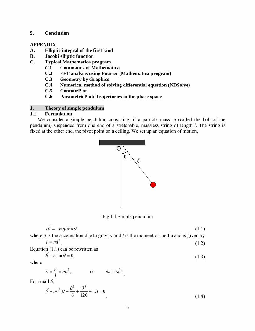
We consider a simple pendulum consisting of a particle mass m (called the bob of the pendulum) suspended from one end of a stretchable, massless string of length l. The string is fixed at the other end, the pivot point on a ceiling. We set up an equation of motion,

Fig.1.1 Simple pendulum

θθ sinmglI −=&& . (1.1) where g is the acceleration due to gravity and I is the moment of inertia and is given by

2mlI = . (1.2) Equation (1.1) can be rewritten as

0sin =+ θεθ&& . (1.3) where

20ωε ==

lg , or εω =0 .

For small θ,

0...)1206

(33

20 =++−+

θθθωθ&&. (1.4)

4

The solution of this equation is given by the nonlinear terms ...)5cos()3cos()cos( 531 ++++++= δωαδωαδωαθ ttt (1.5)

where 321 ααα >> and δ is a phase factor;

192241

91

)16

1()16

1(22

)811(

313

12

020

23

2

0

2

0

21

20

2

ααωωω

α

ααωπ

ωπ

αωω

−≈+−

≈

+=+==

−=

TT

, (1.6) with

glT π

ωπ 22

00 == . (1.7)

In the limit of θ →0, we have 02

0 =+ θωθ&& , (1.8) which corresponds to a simple harmonics,

)cos( 01 δωαθ += t . (1.9) 1.2. Energy conservation and potential energy

The multiplication of θ&on both sides and integration with respect to t lead to 0sin =+ θθεθθ &&&& , (1.10)

or

0)]cos1(21[ 2 =−+ θεθ&

dtd

,

or

)cos1(21

)cos1(21

2

2

θε

θεθ

−+=

−+=

v

E &

, (1.11) where θ&=v , and the first term is the kinetic energy and the second term is a potential energy defined by

)cos1( θε −=U . (1.12)

5

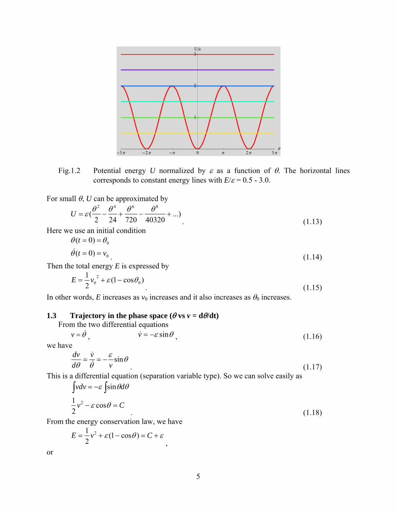
Fig.1.2 Potential energy U normalized by ε as a function of θ. The horizontal lines corresponds to constant energy lines with E/ε = 0.5 - 3.0.

For small θ, U can be approximated by

...)40320720242

(8642

+−+−=θθθθεU

. (1.13)

Here we use an initial condition

0

0

)0(

)0(

vt

t

==

==

θ

θθ&

. (1.14)

Then the total energy E is expressed by

)cos1(21

02

0 θε −+= vE. (1.15)

In other words, E increases as v0 increases and it also increases as θ0 increases. 1.3 Trajectory in the phase space (θ vs v = dθ/dt)

From the two differential equations θ&=v , θε sin−=v& , (1.16)

we have

θεθθ

sinv

vddv

−== &&

. (1.17) This is a differential equation (separation variable type). So we can solve easily as

Cv

dvdv

=−

−= ∫∫θε

θθε

cos21

sin

2

. (1.18) From the energy conservation law, we have

εθε +=−+= CvE )cos1(21 2

,

or

-3 p -2 p -p 0 p 2 p 3 pq

1

2

3Uêe

6

ε−= EC . Now we consider the trajectory in the phase space (θ vs v) for

Ev =−+ )cos1(21 2 θε

. (1.19) Figure 1.3 shows the trajectory in the phase space (θ vs v) for Eq.(1.19), where ε = 1 and the parameter E is changed as a parameter. The character of the trajectories changes from a closed orbit for E<2ε to an open orbit for E>2ε. The curve with E = 2ε is called a separatrics.

Fig.1.3 Trajectories in the phase space (v vs θ) for ε = 1. E = 0.5, 1.0, 1.5, 2.0, 2.5, 3.0,

and 3.5. E = 2ε = 2 is the highest energy of the potential. In Eq.(1.17), both the numerator and the denominator becomes zero at the singular points [v = 0 and θ = nπ (n = 0, ±1, ±2, …)]. We consider the motion near the singular points by putting

ξπθ =− n ( 0≈ξ ). (1.20) For n = even, we have

εξξεπξεξ

−=−=+−==

sin)sin( nvv&

& , (1.21)

which is equivalent to the equation of the simple harmonics. Then the singular points are called stable spiral points. For n = odd, we have

εξξεπξεπξεξ

==+−=+−==

sin)sin()sin( nvv&

&

7

or

vv

ddv ξε

ξξ== &

&

(1.22) or

122

21 Cv =− εξ , (1.23)

where C1 is constant. The singular points are called saddle points. Figure 1.4 shows the motion near the saddle point (ξ = 0, v = 0).

Fig.1.4 Trajectories in the phase space (v vs ξ) for ε = 1, which is the contour plot of Eq.(1.18) with C1 being changed as a parameter.

2. Exact solution of simple pendulum using Jacobi elliptic function (k<1) 2.1 Differential equation for the motion

We consider the energy conservation given by 2

02

21)cos1(

21 vvE =−+= θε

. (2.1) We assume that

v = 0, when θ = θmax. So we have

2sin2)cos1(

21)cos1(

21 max2

max2

02 θεθεθε =−==−+= vvE .

From this, we get

8

)cos(cos

)cos1()cos1(21

max22

max2

θθεθ

θεθε

−==

−+−−=

&v

v

. (2.2) Using a formula,

2sin21cos 2 θθ −=

,

we have

2sin

2sin2 2max2 θθεθθ −==

dtd&

, (2.3)

or

∫∫∫−

=−

==θθ

ϕϕ

ϕθϕεε

0 22

0 2max20

2sin11

21

2sin

2sin

21'

k

dk

dtdtt

, (2.4) where

tu ε= and )2

sin( maxθ=k

. (2.5)

In Eq.(2-4), we put

2sin1 ϕξ

k= ,

leading to

ϕξϕϕξ dkk

dk

d 22121

2cos

21

−==,

or

2212

ξξϕ

kkdd−

=.

When ϕ is equal to θ in Eq.(2.4), the upper limit of ξ is

2sin1sin θφ

kz == . (2.6)

Then Eq.(2-4) can be rewritten as

∫ −−=

z

kdu

0222 11 ξξ

ξ

, (2.7)

or in the form of differential equation, as

222 111

zkzdzdu

−−=

. (2.8) Using the relation,

φφφ

ddzz

cossin

==

,

du can be rewritten as

9

φφ

22 sin1 kddu

−=

, (2.9)

or in the differential form, as

φφ 22 sin11

kddu

−=

. (2.10)

2.2 Jacobi elliptic function

Here we introduce the Jacobi elliptic functions. These functions are defined as follows (see the Appendix for the detail).

)(sin usnz == φ , (2.11) )(1sin1cos)( 22 usnucn −=−== φφ , (2.12)

and

)()(12

sin12

cos

)(2

sin

222 udnusnk

usnk

=−=−=

⋅=

θθ

θ

, (2.13) where

1)()( 22 =+ ucnusn . (2.14) Using the relation

)()(1sin1 2222 udnusnkkdud

=−=−= φφ

, (2.15) we have

)()()(1)(

)()()cos()(

)()()sin()(

222

ucnusnkdu

usnkddu

uddn

udnusndu

ddu

udcn

udnucndu

ddu

udsn

−=−

=

−==

==

φ

φ

, (2.16) 2.3. Expression for the angle as a function of time

For k<1, we get an exact expression for the angle of the single pendulum,

),(2

sin1sin ktusnk

z εθφ ====, (2.17)

or )],(sin[2 ktusnkArc εθ =⋅= . (2.18)

The angle θ is a single-valued function of t. From Eq.(2.18), dtd /θ can be calculated as

10

).(),(),(21

2cos kudnkucnk

dtdukusn

dudk ⋅=⋅⋅=⋅ εθθ &

, (2.19) or

),(),(2 0 ktucnvktucnkv εεεθ ===⋅== &, (2.20)

where 2max22

0 22

sin221 kvE εθε === . (2.21)

or

021 vk

ε= (<1). (2.22)

We note that from the relation, 1)()( 22 =+ ucnusn , we get the energy conservation law for the pendulum,

20

2

21)cos1(

21 vv =−+ θε . (2.23)

For k = 1, we have

)tanh()1,(2

sin tutusn εεθ====

, (2.24)

or )]sin[tanh(2 tuArc εθ == . (2.25)

When t→∞, θ become π. This means that it takes infinity-time for θ to change from θ = 0 to θ = π. ((Example)) Calculation of θ vs t. ε = 1. v0 is changed as a parameter.

Fig.2.1 Plot of θ vs t. ε = 1. v0 = 1.7 (red), 1.75 (yellow), 1.80 (green), 1.85 (blue), 1.90 (purple), and 1.95.

11

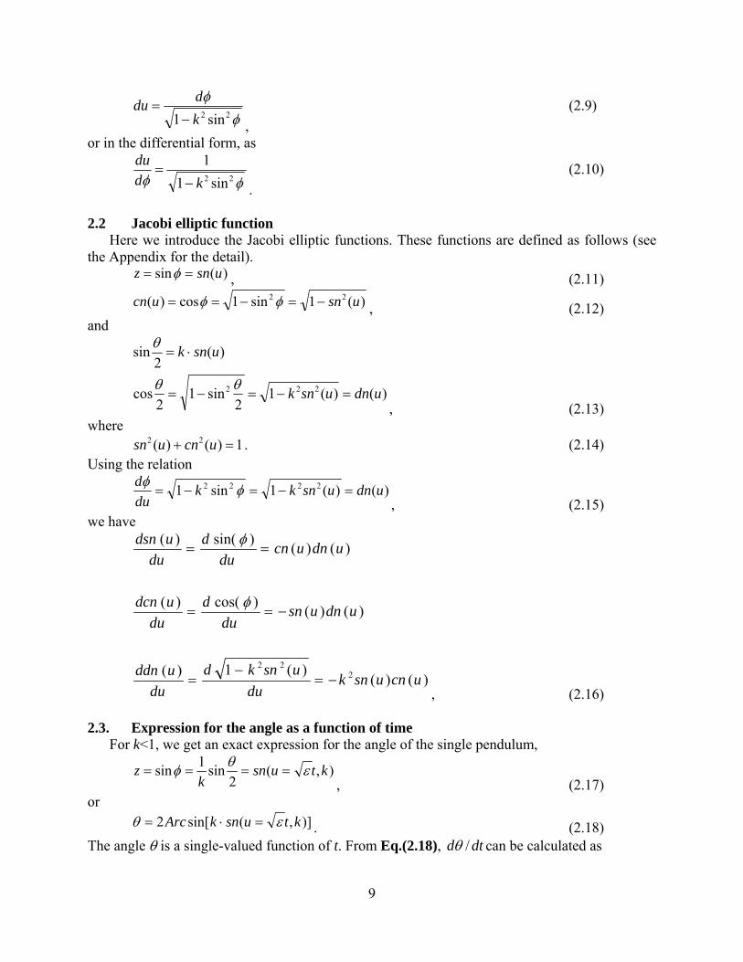
Fig.2.2 Plot of θ vs t. ε = 1. v0 = 1.995 (red), 1.996 (yellow), 1.997 (green), and 1.998 (blue).

Fig.2.3 Plot of θ vs t. ε = 1. v0 = 1.9990 (red), 1.9992 (yellow), 1.9994 (green), and 1.9996 (blue).

12

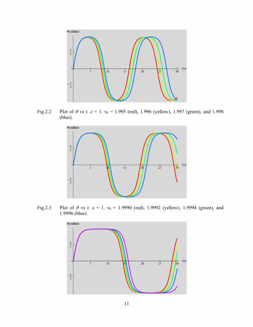
Fig.2.4 Plot of θ vs t. ε = 1. v0 = 1.999990 (red), 1.999992 (yellow), 1.999994 (green),

1.999996 (blue), and 1.999998 (blue). 2.4 Wave analysis by Fast Fourier transform

The sine wave is formed at small vo. The form of the sine wave is deformed as vo increases. In the vicinity of v0 ≈ 2, the form changes from the sine wave to a square wave, indicating the enhancement of effects from higher order harmonics. The frequency of the first harmonic is reduced to zero at v0 = 2. Using the fast Fourier transform (FFT), we analyze how the higher order terms due to the nonlinearity of the system is enhanced when v0 approaches 2. (a) v0 = 0.2

Fig.2.5 The square of amplitude in FFT Fourier spectrum vs ω (rad/s). ε = 1. v0 = 0.2

(b) v0 = 1.60

Fig.2.6 The square of amplitude in FFT Fourier spectrum vs ω (rad/s). ε = 1. v0 = 1.6.

0 1 2 3 4 510-8

10-6

10-4

0.01

1

100

1040.2

0 1 2 3 4 510-4

0.01

1

100

104

1.6

13

(c) v0 = 1.92

Fig.2.7 The square of amplitude in FFT Fourier spectrum vs ω (rad/s). ε = 1. v0 = 1.92.

(d) v0 = 1.98

Fig.2.8 The square of amplitude in FFT Fourier spectrum vs ω (rad/s). ε = 1. v0 = 1.98. (e) v0 = 1.998

0 1 2 3 4 510-4

0.01

1

100

104

1.92

0 1 2 3 4 510-4

0.01

1

100

104

1.98

14

Fig.2.9 Fourier spectrum of the square of amplitude vs ω (rad/s). ε = 1. v0 = 1.998

2.5 Trajectories in the phase space (v vs θ)

Fig.2.10 Trajectories in the phase space of θ vs v. ε = 1. v0 is changes as a parameter. v0 = 1.80 (red), 1.85 (yellow), 1.90 (Green), and 1.95 (blue).

0 1 2 3 4 510-4

0.01

1

100

104

1.998

15

Fig.2.11 Trajectories in the phase space of θ vs v. ε = 1. v0 is changes as a parameter. v0 = 1.96 (red), 1.97 (yellow), 1.98 (Green), and 1.99 (blue).

2.6 Period T

Noting that tu ε= , the period T is given by

)(42 kKTεω

π==

. (2.26) where K(k) is the complete elliptic integral of the first kind and is defined by

∫ −−=

1

0222 11

)(ξξ k

dzkK (= EllipticK[m (= k2)]). (2.27)

We note that K(k) can be also defined as

∫ −=

2/

022 sin1

)(π

ϕϕ

kdkK

. (2.28) The complete elliptic integral of the first kind is implemented in Mathematica as EllipticK[m (= k2)]. Note the use of the parameter m = k2 instead of the modulus k. The parameter k is related to vo and ε as

021 vk

ε= , (2.29)

because of the energy conservation given by 2max2

max2

0 22

sin2)cos1(21 kv εθεθε ==−=

. (2.30) In summary, ω is given by

)2

(

12 0

ε

επω vkK ==

. (2.31)

16

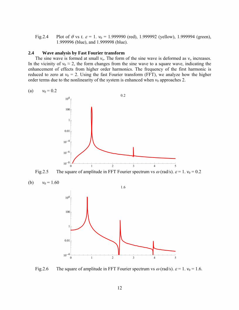
Here we show the result of calculation of ω as a function of v0. For simplicity, we assume that ε = 1. We make a plot of ω vs v0 for ε = 1. Note that

0lim020

=−→

ωv . (2.32)

Fig. 2.12 Plot of ω vs v0 for ε = 1. The angular frequency reduces to zero at v0 = 2.

Fig. 2.13 Plot of ω vs v0 for ε = 1. The angular frequency reduces to zero at v0 = 2.

0. 0.5 1. 1.5 2.v00.

0.2

0.4

0.6

0.8

1.w

1.9 1.91 1.92 1.93 1.94 1.95 1.96 1.97 1.98 1.99 2.v00.

0.2

0.4

0.6

w

17

Fig.2. 14 Plot of ω vs v0 for ε = 1. The angular frequency reduces to zero at v0 = 2. 2.7 The behavior of ω in the vicinity of v0 = 2 for ε = 1.

We consider the value of ω in the vicinity of the critical value v0 = 2. For convenience we introduce the parameter t which is defined by

tv −= 20 . (2.33) Note that t is not a time. Then the critical behavior of ω can be expressed by

)2

1(

12)

2(

12 0 tkKvkK −=

==

=π

ε

πω

. (2.34) around t = 0, where ε = 1. Using the Mathematica, it can be easily demonstrated that

]4[]1[ 2/1−≈− tLogtEllipticK , (2.35) in the limit of t→0. This approximation in the Mathematica can be rewritten as

)4ln()2

1()1( 2/1−≈−=≈−= ttkKtkK, (2.36)

in the standard form. Using this formula, we find that ω (=ωl) tends to zero as

)4ln(1

2 2/1−≈=tl

πωω, (2.37)

in the limit of t→0, where l stands for lower.

1.99 1.995 2.v0

0.2

0.3

0.4

w

18

Fig.2.15 ω (rad/s) vs t (t = = 2 - v0) in the vicinity of v0 = 2. ε = 1. 2.8 θmax vs v0

The maximum angle θmax is related to v0 as

)2

arcsin(2)arcsin(2 0max ε

θ vk ==. (2.38)

We make a plot of θmax vs v0 for ε = 1 (denoted by red curve). For comparison we also show a plot of the straight line (denoted by a blue line); εθ /2 0max v= . The red curve almost coincides with the blue line for v0<0.8. This difference becomes large when v0 tends to 2 from the smaller side of v0.

Fig.2.16 Plot of θmax vs v0 (red) for ε = 1. The blue line is a prediction of θmax vs v0 in the

small angle limit approximation. 3. Exact solution for k>1 3.1 Time dependence of the rotation angle

We now discuss the case when E>2ε,

10-12 10-9 10-6 0.001 1t=H2-v0L

0.2

0.4

0.6

0.8

w

0.5 1. 1.5 2.v0

p4

p2

3 p4

p

qmax

19

εθεθε 221

2sin2

21)cos1(

21 2

0222 >=+=−+= vvvE

, (3.1) In this case, the bob with a mass m continues to rotate. From Eq.(3.1), we get a differential equation for θ,

2sin4 22

0θεθ −== vv &

. (3.2) Here we introduce a new parameter κ defined by

112

0

<==kv

εκ. (3.3)

Then we get

2sin12 22 θκ

κεθθ −==

dtd&

. (3.4) This equation can be rewritten as

∫−

=θ

ϕκ

ϕκ

ε

0 22

2sin1

2 dt

. (3.5) We put

ϕξϕϕξ

ϕξ

ddd 2121

2cos

21

2sin

−==

=

. (3.6) Then we get

∫ −−==

)2/sin(

02222 11

θ

ξκξκϕ

κε dut

. (3.7) The solution of Eq.(3.7) is given by a Jacobi elliptic function

),(),(2

sin κκεκθ tsnusn ==

. (3.8) ((Note))

),(1),(

),(1),(22

2

κκκ

κκ

usnudn

usnucn

−=

−=

. (3.9) The angle θ is a multi-valued function of t. We make a plot of θ vs t using a ContourPlot (Mathematica). We assume that ε = 1.

20

Fig.3.1 Plot of θ (rad) vs t (s) for v0 = 2.3. The appropriate curve passes through the origin among a family of curves.

Fig.3.2 Plot of θ (rad) vs t (s) for v0 = 2.1. The appropriate curve passes through the origin among a family of curves.

0 5 10 15 20 25 300

10

20

30

40

50

60

2.3

0 5 10 15 20 25 300

10

20

30

40

50

60

2.1

21

Fig.3.3 Plot of θ (rad) vs t (s) for v0 = 2.01. The appropriate curve passes through the origin among a family of curves.

3.2 Period T

The period T is calculated in the following way.

∫∫ −=

−=

2/

022

0 22 sin14

2sin1

22 ππ

ϕκϕ

ϕκ

ϕκ

ε ddT

, (3.10) or

)(2sin1

2 2/

022

κεκ

ϕκϕ

εκ π

KdT =−

= ∫. (3.11)

The angular frequency ω is obtained as

)(12κκ

εππωKT

==. (3.12)

We make a plot of ω vs v0 for ε = 1, where 00

22vv

==εκ and v0>2. We note that

0lim020

=+→

ωv . (3.13)

0 5 10 15 20 25 300

10

20

30

40

50

60

2.01

22

Fig.3.4 Plot of ω vs v0 for v0>2. ε = 1. 00

22vv

==εκ

.

3.3 Critical behavior of ω vs v0 in the vicinity of v0 = 2

We consider the value of ω in the vicinity of the critical value v0 = 2 (v0>2). For convenience we use the parameter t defined by

tv += 20 . (3.14) where t is not a time. Then the parameter κ is given by

21

22 t

t−≈

+=κ

for ε = 1. The critical behavior of ω around t = 0 is described by

)2

1()2

1(

1

21 tKtKt

−=≈

−=−=

κ

π

κ

πω

. (3.15) Here we use the approximation given by

)4ln()2

1()1( 2/1−≈−=≈−= ttKtK κκ, (3.16)

in the limit of t→0. Then ω (= ωu) tends to zero as

)4ln(1

2/1−≈=tu πωω

, (3.17) in the limit of t→0, where the subscript u stands for upper. Note that the ratio ωu/ωl = 2 at the same t, indicating the asymmetric behavior of ω with respect to the axis of v0 = 2. We show the plot of ω vs t where t = v0 -2.

2.0 2.1 2.2 2.3 2.4 2.5v00.0

0.5

1.0

1.5

2.0w radês

23

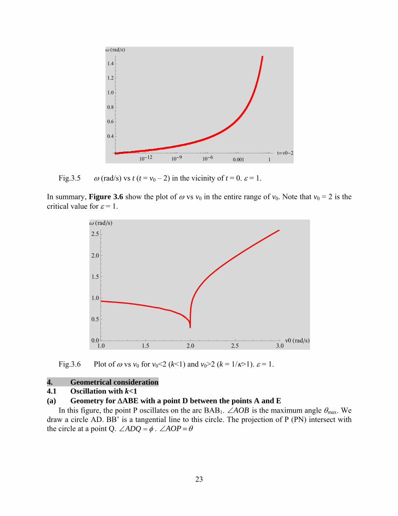
Fig.3.5 ω (rad/s) vs t (t = v0 – 2) in the vicinity of t = 0. ε = 1. In summary, Figure 3.6 show the plot of ω vs v0 in the entire range of v0. Note that v0 = 2 is the critical value for ε = 1.

Fig.3.6 Plot of ω vs v0 for v0<2 (k<1) and v0>2 (k = 1/κ>1). ε = 1. 4. Geometrical consideration 4.1 Oscillation with k<1 (a) Geometry for ΔABE with a point D between the points A and E

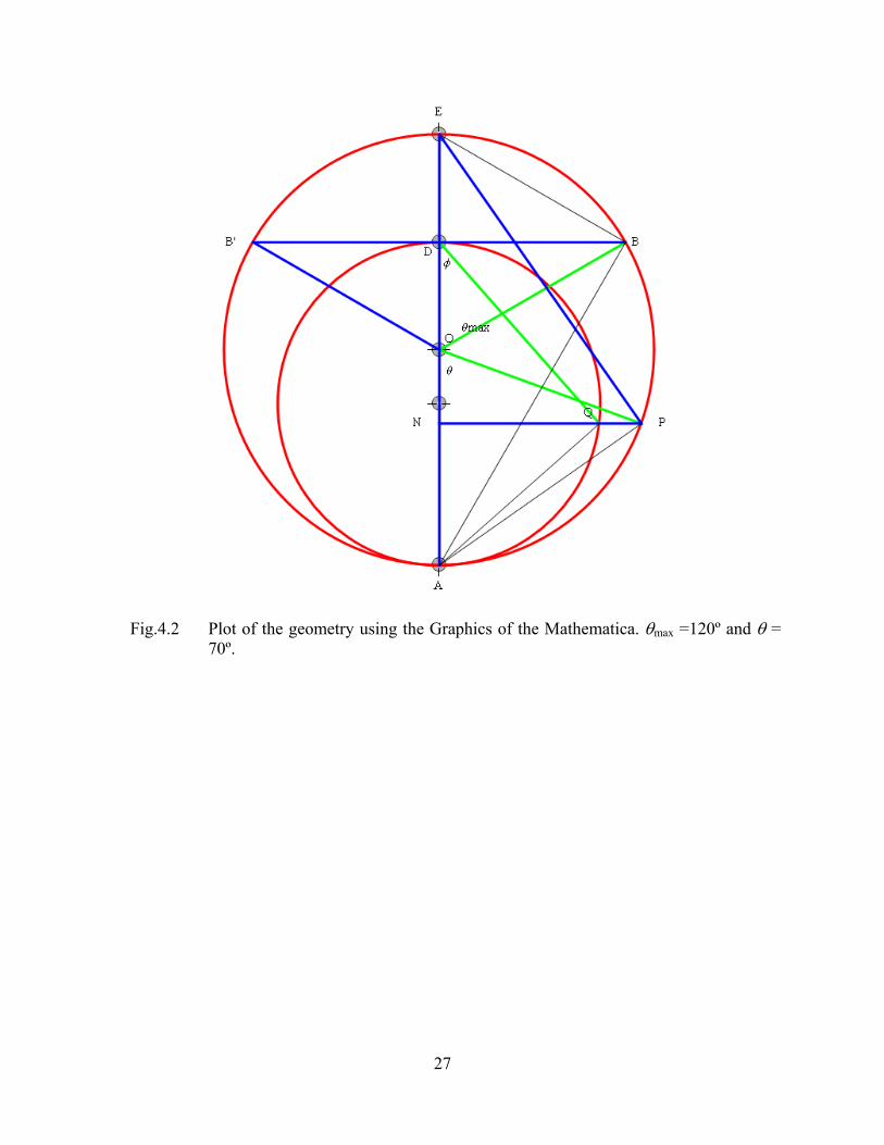
In this figure, the point P oscillates on the arc BAB1. AOB∠ is the maximum angle θmax. We draw a circle AD. BB’ is a tangential line to this circle. The projection of P (PN) intersect with the circle at a point Q. φ=∠ADQ . θ=∠AOP

10-12 10-9 10-6 0.001 1t=v0-2

0.4

0.6

0.8

1.0

1.2

1.4

w HradêsL

1.0 1.5 2.0 2.5 3.0v0 HradêsL0.0

0.5

1.0

1.5

2.0

2.5

w HradêsL

24

Fig.4.1 Plot of the geometry using the Graphics of the Mathematica. θmax =80º and θ = 50º.

First we consider the geometrical relations for ΔABE with a point D between the points A and E

2maxmax

2max

max

max

max

max

122

cos22

cos

22

sin

22

sin

2212

21

kllAEBE

lkABAD

lkAEAB

lOBlAE

ABD

ABE

AEB

AOB

−==⋅=

=⋅=

=⋅=

==

=∠

=∠

=∠

=∠

θθ

θ

θ

θ

π

θ

θ

,

(4.1)

where

25

2sin maxθ

=k and 2max 12

cos k−=θ . (4.2)

We note that ΔABE is similar to ΔADB. This leads to the following relation,

AEAB

ABADk == , or

AEAD

AEAB

ABADk ==2 . (4.3)

(b) Geometry for ΔAEP with a point N between the points A and E We consider the geometrical relations for ΔAEP with a point N between the points A and E

)()(22

cos

)(2)](1[2)(2)](1[2

)(22

sin22

sin

)(22

sin22

sin

22

sin2)cos1(

)(22

cos22

cos

212

21

222

2222

222

2max2max

udnusnlkAPNP

udnlusnklANAEENucnlkusnlkANADND

usnlklAPAN

usnlklAEAP

lkllDOAOAD

udnllAEEP

APN

APE

AEP

AOP

⋅⋅=⋅=

⋅=⋅−⋅=−=

⋅=−⋅=−=

⋅=⋅=⋅=

⋅=⋅=⋅=

=⋅=−⋅=−=

⋅=⋅=⋅=

=∠

=∠

=∠

=∠

θ

θθ

θθ

θθ

θθ

θ

π

θ

θ

. (4.4)

We note that ΔPEN is similar to ΔAPN. This leads to the relation

ANNP

NPEN

=, (4.5)

or )()(4)(2)(2 22222222 usnudnklusnlkudnlANENNP ⋅=⋅⋅⋅=⋅= . (4.6)

(c) Geometry for ΔADQ with a point N between the points A and D

We consider the geometrical relation for ΔADQ with a point N between the points A and D

26

)()(2cossin2cos)(2sin2sinsin

)(2sin2sin

2

22

22222

22

ucnusnlklkAQNQusnlklkADAQAN

usnlklkADAQAQN

AQD

ADQ

⋅==⋅=

⋅=⋅=⋅=⋅=

⋅=⋅=⋅=

=∠

=∠

=∠

φφφ

φφφ

φφ

φ

πφ

. (4.7)

We note that ΔDNQ is similar to ΔQNA. This leads to the relation

ANNQ

NQDN

=, (4.8)

or )(2)(2 22222 usnlkucnlkANDNNQ ⋅⋅⋅=⋅= , (4.9)

or )()(2 2 ucnusnlkNQ ⋅⋅= . (4.10)

(d) Relation between θ and φ

From the above consideration, we have the relation, the length AN is described by φ22 sin2 ⋅= lkAN , (4.11)

in terms of φ. The length AN is also described by

2sin2 2 θlAN =

, (4.12) in terms of θ. From these relations, we obtain

zk =⋅= φθ sin2

sin. (4.13)

((Example))

27

Fig.4.2 Plot of the geometry using the Graphics of the Mathematica. θmax =120º and θ = 70º.

28

Fig.4.3 Plot of the geometry using the Graphics of the Mathematica. θmax = 150º, θ = 70º. 4.2 k = 1 (critical state)

The circle AD coincides with the circle AE.

)(sec)1,(cos

)tanh()1,(sin2

sin

2

uhkucn

ukusn

===

====

=

φ

φθ

φθ

(4.14),

where ukusn tanh)1,( == ,

29

)(sec)tanh(2)1,()1,(2cossin2cos

tanh2)1,(22

sin2sin2sin

)tanh(2)1,(22

sin2sin2

2

2222

uhulkucnkusnllAPNP

ulkusnlllAPAN

ulkusnlllAP

APN

OEP

AOP

⋅⋅==⋅=⋅=⋅=⋅=

⋅==⋅=⋅=⋅=⋅=

⋅==⋅=⋅=⋅=

=∠

=∠

=∠

φφφ

θφφ

θφ

φ

φθ

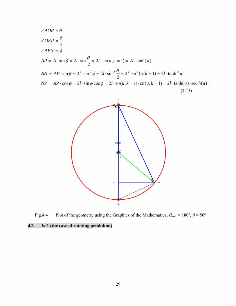
, (4.15)

Fig.4.4 Plot of the geometry using the Graphics of the Mathematica. θmax = 180º, θ = 50º 4.3. k>1 (the case of rotating pendulum)

30

Fig.4.5 Plot of the geometry using the Graphics of the Mathematica. κ = 0.90 and θ = 70°.

From the energy conservation law, 2

02

21)cos1(

21 vvE =−+= θε

, (4.16) the angular velocity at the point E (θ = π) can be calculated as

εθ 420 −== vv &

. (4.17) We note that the velocity at the point E is

ε420 −== vllvVE . (4.18)

We choose the point D such that the velocity Vff at the point E after the free fall from the point D is equal to the velocity VE when it reaches at the top of the circle (the point E). The distance DE is related to the velocity Vff at the point E is

lV

gV

DE ffff

ε

22

2==

, (4.19) where ε = g/l or g = εl and Vff = VE. Then the distance is rewritten as

)11(22

)44(

2)4(

2

2220 −=

−=

−=

κε

εκ

ε

εε l

l

llvDE

, (4.20)

31

where

κε2

0 =v. (4.21)

Then the distance AD is given by

222)11(22κκ

lllDEAEAD =−+=+=. (4.22)

From the above figure, we have the following relations.

),(),(sin2

sin

2

κεκφθ

φθ

tsnusn ===

=. (4.23)

lAEucnusnlAEAPNP

udnlusnlllANADDN

ucnlAEEPENusnlAEAPAN

ucnlAEEPusnlAEAP

2),(),(2cossincos

),(2)),(1(2sin22),(2coscos),(2sinsin

),(2cos),(2sin

22

222

22

22

22

=⋅=⋅=⋅=

⋅=−=⋅−=−=

⋅=⋅=⋅=

⋅=⋅=⋅=

⋅=⋅=⋅=⋅=

κκφφφ

κκ

κκκ

φκ

κφφ

κφφ

κφκφ

. (4.24)

5. Numerical calculation using Mathematica for simple pendulum

Here we show the numerical calculation using Mathematica. We use NDSolve to solve the nonlinear differential equation with the appropriate initial conditions. The advantage of this method is that we do not need any mathematical knowledge on the Jacobi elliptic functions. It is interesting to compare our numerical calculations with the results obtained from the exact solutions above described. 5.1 Formulation

For convenience, the differential equation is separated into two parts θ&=v θε sin−=v& . (5.1)

1. First we solve this differential equation using numerical method (Mathematica, NDSolve)

2. We analyze the Fourier component by using the fast Fourier transform (FFT) (Mathematica , Fourier). a. We choose the N (= 2n) data, typically the data between 0 and T (= tmax). b. The minimum time division is NT /=Δ , which corresponds to the maximum wmax

given by

NTπω 2

max =. (5.2)

c. The Fourier spectrum is plotted as a function of the angular frequency defined by channel number multiplied by (2p)/T.

32

For simplicity, we consider the case of θ0 = 0. Then we have 2

021 vE =

(5.3) When v0<2 ε (or E<2ε), the value of θ is limited between –π and π. When v0>2 ε (or E>2ε), the value of θ is unlimited. 5.2 Time dependence (θ vs t)

We show the time dependence of θ as a function of t with v0 being changed as a parameter. Here we choose. ε = 1. (a) v0 = 0.1, 0.2, 0.3, 0.4, 0.5

Fig.5.1 Time dependence of θ. ε = 1. v0 is changed as a parameter: v0 = 0.1 (red), 0.2 (yellow), 0.3 (light green), 0.4 (blue), and 0.5 (purple).

(b) v0 = 1.4, 1.5, 1.6

Fig.5.2 Time dependence of θ. ε = 1. v0 is changed as a parameter: v0 = 1.4 (red), 1.5 (light green), and 1.6 (blue).

10 20 30 40 50t

- p6

p6

q

10 20 30 40 50 60 70 80 90 100t

- p4

p4

q

33

(c) v0 = 1.91, 1.92, 1.93

Fig.5.3 Time dependence of θ. ε = 1. v0 is changed as a parameter: v0 = 1.91 (red), 1.92 (light green), and 1.93 (blue).

(d) v0 = 1.982, 1.984, 1.986, 1.988, 1.990

Fig.5.4 Time dependence of θ. ε = 1. v0 is changed as a parameter: v0 = 1.982 (red), 1.984 (brown), 1.986 (light green), 1.988 (dark green), and 1.990 (blue).

(e) v0 = 1.9992, 1.9993, 1.9994, 1.9995, 1.9996, 1.9997

10 20 30 40 50 60 70 80 90 100t

- 3 p4

- p2

- p4

p4

p2

3 p4

q

10 20 30 40 50 60 70 80 90 100t

- 3 p4

- p2

- p4

p4

p2

3 p4

q

34

Fig.5.5 Time dependence of θ. ε = 1. v0 is changed as a parameter: 1.9992 (red), 1.9993, 1.9994, 1.9995, 1.9996, 1.9997 (green)

(f) v0 = 1.999992, 1.999993, 1.999994, 1.999995, 1.999996, 1.999997, 1.999998, 1.999999

As v0 approaches 2.0, the shape of θ vs t curve becomes square-like. This means that the effect of the nonlinearity is enhanced.

Fig.5.6 Time dependence of θ. ε = 1. v0 is changed as a parameter: v0 = 1.999992 (red), 1.999993, 1.999994, 1.999995, 1.999996, 1.999997, 1.999998, 1.999999 (purple)

(g) v0 = 2

In this case, the total energy E is equal to the peak height of the potential energy. This is a result form the computer calculation. This result does not agree with the theoretical prediction. Nevertheless we show this result here, indicating that the numerical calculation may be wrong in such a critical condition (v0 = 2.0).

10 20 30 40 50 60 70 80 90 100t

-p

- 3 p4

- p2

- p4

p4

p2

3 p4

p

q

10 20 30 40 50 60 70 80 90 100t

-p

- p2

p2

p

q

35

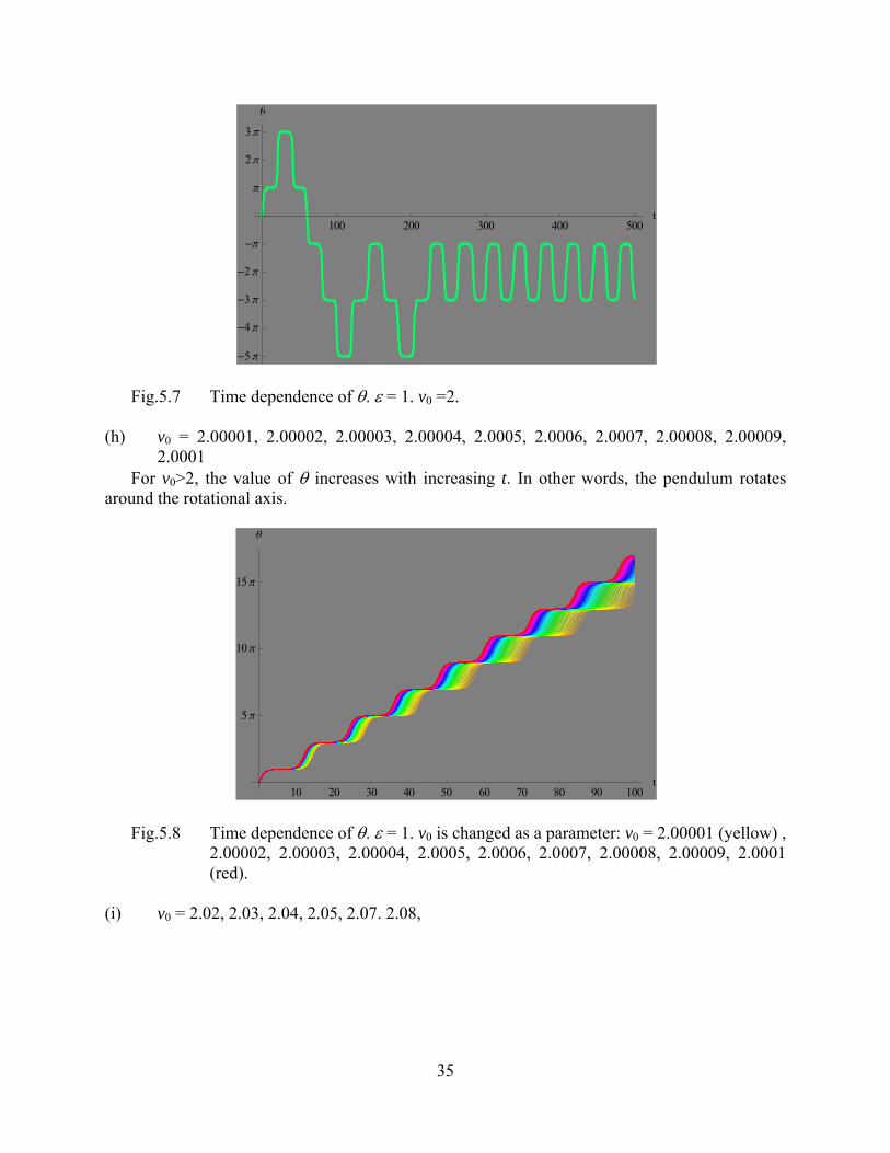
Fig.5.7 Time dependence of θ. ε = 1. v0 =2. (h) v0 = 2.00001, 2.00002, 2.00003, 2.00004, 2.0005, 2.0006, 2.0007, 2.00008, 2.00009,

2.0001 For v0>2, the value of θ increases with increasing t. In other words, the pendulum rotates

around the rotational axis.

Fig.5.8 Time dependence of θ. ε = 1. v0 is changed as a parameter: v0 = 2.00001 (yellow) , 2.00002, 2.00003, 2.00004, 2.0005, 2.0006, 2.0007, 2.00008, 2.00009, 2.0001 (red).

(i) v0 = 2.02, 2.03, 2.04, 2.05, 2.07. 2.08,

100 200 300 400 500t

-5 p

-4 p

-3 p

-2 p

-p

p

2 p

3 p

q

10 20 30 40 50 60 70 80 90 100t

5 p

10 p

15 p

q

36

Fig.5.9 Time dependence of θ. ε = 1. v0 is changed as a parameter: v0 = 2.02 (red), 2.03, 2.04, 2.05, 2.07. and 2.08 (blue).

(j) v0 = 2.10, 2.12, 2.14, 2.16, 2.18. and 2.20

Fig.5.10 Time dependence of θ. ε = 1. v0 is changed as a parameter: v0 = 2.10 (red), 2.12, 2.14, 2.16, 2.18. and 2.20 (blue).

5.3 Trajectories in the phase space (v vs θ)

Figure shows the trajectories in the phase space (v vs θ) for ε = 1, when v0 is changed as a parameter. (a) v0 = 1.0, 1.1, 1.2, 1.3, 1.4, 1.5

10 20 30 40 50 60 70 80 90 100t

10 p

20 p

30 p

q

10 20 30 40 50 60 70 80 90 100t

10 p

20 p

30 p

40 p

q

37

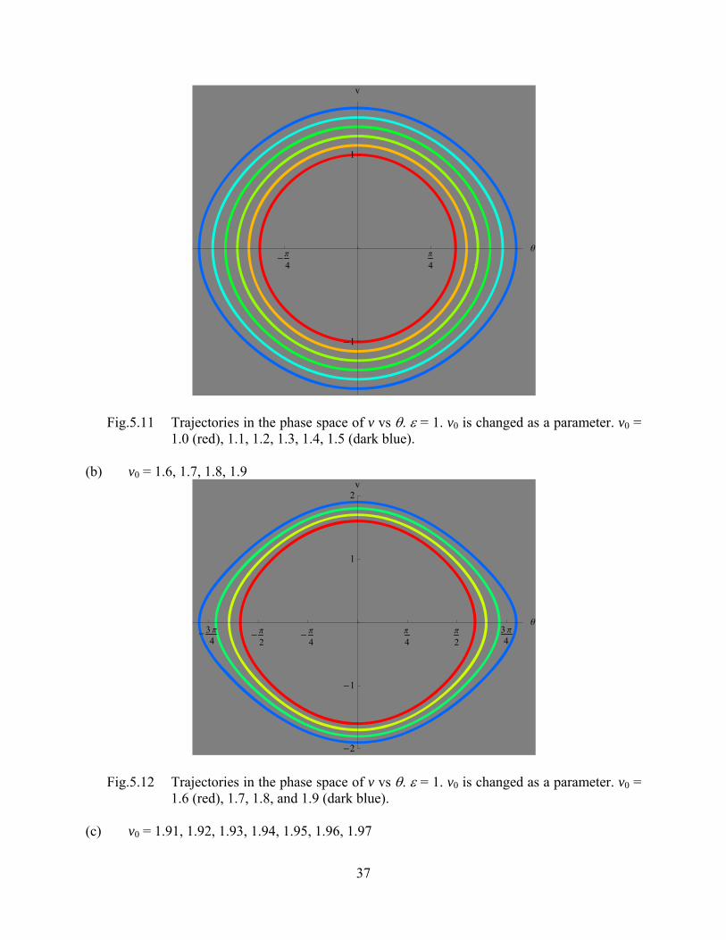
Fig.5.11 Trajectories in the phase space of v vs θ. ε = 1. v0 is changed as a parameter. v0 = 1.0 (red), 1.1, 1.2, 1.3, 1.4, 1.5 (dark blue).

(b) v0 = 1.6, 1.7, 1.8, 1.9

Fig.5.12 Trajectories in the phase space of v vs θ. ε = 1. v0 is changed as a parameter. v0 = 1.6 (red), 1.7, 1.8, and 1.9 (dark blue).

(c) v0 = 1.91, 1.92, 1.93, 1.94, 1.95, 1.96, 1.97

- p4

p4

q

-1

1

v

- 3 p4

- p2

- p4

p4

p2

3 p4

q

-2

-1

1

2v

38

Fig.5.13 Trajectories in the phase space of v vs θ. ε = 1. v0 is changed as a parameter. v0 = 1.91 (red), 1.92, 1.93, 1.94, 1.95, 1.96, 1.97 (purple)

(d) v0 = 1.980, 1,981, 1.982, 1.983, 1.984, 1.985, 1.986, 1.987, 1.988, 1.989, 1.990.

Fig.5.14 Trajectories in the phase space of v vs θ. ε = 1. v0 is changed as a parameter. v0 = 1.980, 1,981, 1.982, 1.983, 1.984, 1.985, 1.986, 1.987, 1.988, 1.989, 1.990.

(e) v0 = 2.0

- 3 p4

- p2

- p4

p4

p2

3 p4

q

-2

-1

1

2v

- 3 p4

- p2

- p4

p4

p2

3 p4

q

-2

-1

1

2

v

39

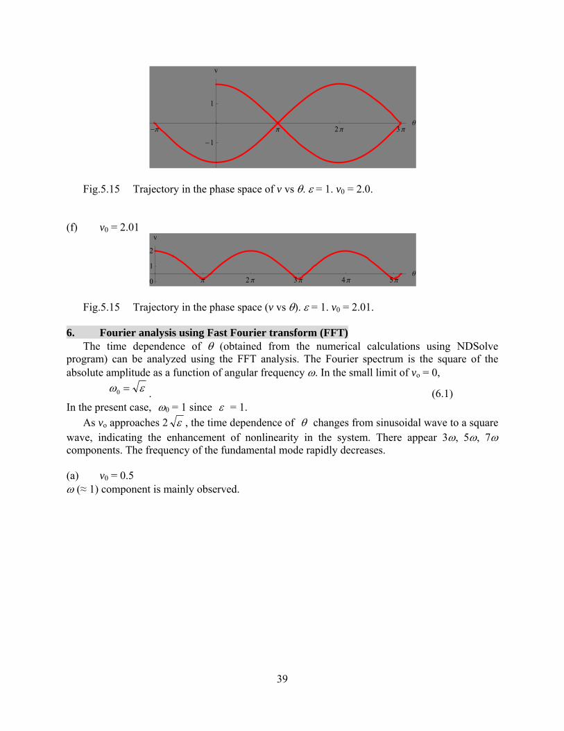
Fig.5.15 Trajectory in the phase space of v vs θ. ε = 1. v0 = 2.0. (f) v0 = 2.01

Fig.5.15 Trajectory in the phase space (v vs θ). ε = 1. v0 = 2.01. 6. Fourier analysis using Fast Fourier transform (FFT)

The time dependence of θ (obtained from the numerical calculations using NDSolve program) can be analyzed using the FFT analysis. The Fourier spectrum is the square of the absolute amplitude as a function of angular frequency ω. In the small limit of vo = 0,

εω =0 . (6.1) In the present case, ω0 = 1 since ε = 1.

As vo approaches 2 ε , the time dependence of θ changes from sinusoidal wave to a square wave, indicating the enhancement of nonlinearity in the system. There appear 3ω, 5ω, 7ω components. The frequency of the fundamental mode rapidly decreases. (a) v0 = 0.5 ω (≈ 1) component is mainly observed.

-p p 2 p 3 pq

-1

1

v

p 2 p 3 p 4 p 5 pq

0

1

2

v

40

Fig.6.1 Fourier spectrum obtained from the FFT analysis of the θ vs t obtained from the numerical calculation using Mathematica. The x axis is the angular frequency ω and the y axis is the squares of the absolute value of complex amplitude. The fundamental harmonic is observed at ω (= 1).

(b) v0 =1.6 ω (<1) and 3ω component are mainly observed.

Fig. 6.2 The FFT spectrum for v0 = 1.6. (c) v0 = 1.9

ω, 3ω, and 5ω component are mainly observed.

0 1 2 3 4 510-5

0.001

0.1

10

1000

0 1 2 3 4 50.001

0.01

0.1

1

10

100

1000

41

Fig. 6.3 The FFT spectrum for v0 = 1.9. (d) v0 = 1.981

ω, 3ω, 5ω, and 7ω component are mainly observed.

Fig. 6.4 The FFT spectrum for v0 = 1.981. (e) v0 = 1.9962

ω, 3ω, 5ω, 7ω, and 9ω component are mainly observed.

0 1 2 3 4 50.001

0.01

0.1

1

10

100

1000

0 1 2 3 4 50.001

0.01

0.1

1

10

100

1000

42

Fig. 6.5 The FFT spectrum for v0 = 1.9962. (f) v0 = 1.9991

ω, 3ω, 5ω, 7ω, 9ω, 11ω, and 13ω component are mainly observed.

Fig. 6.6 The FFT spectrum for v0 = 1.9991. (g) v0 = 1.999995

ω, 3ω, 5ω, 7ω, 9ω, 11ω, 13ω, 15ω, and 17ω component are mainly observed.

0 1 2 3 4 50.001

0.01

0.1

1

10

100

1000

0 1 2 3 4 50.001

0.01

0.1

1

10

100

1000

43

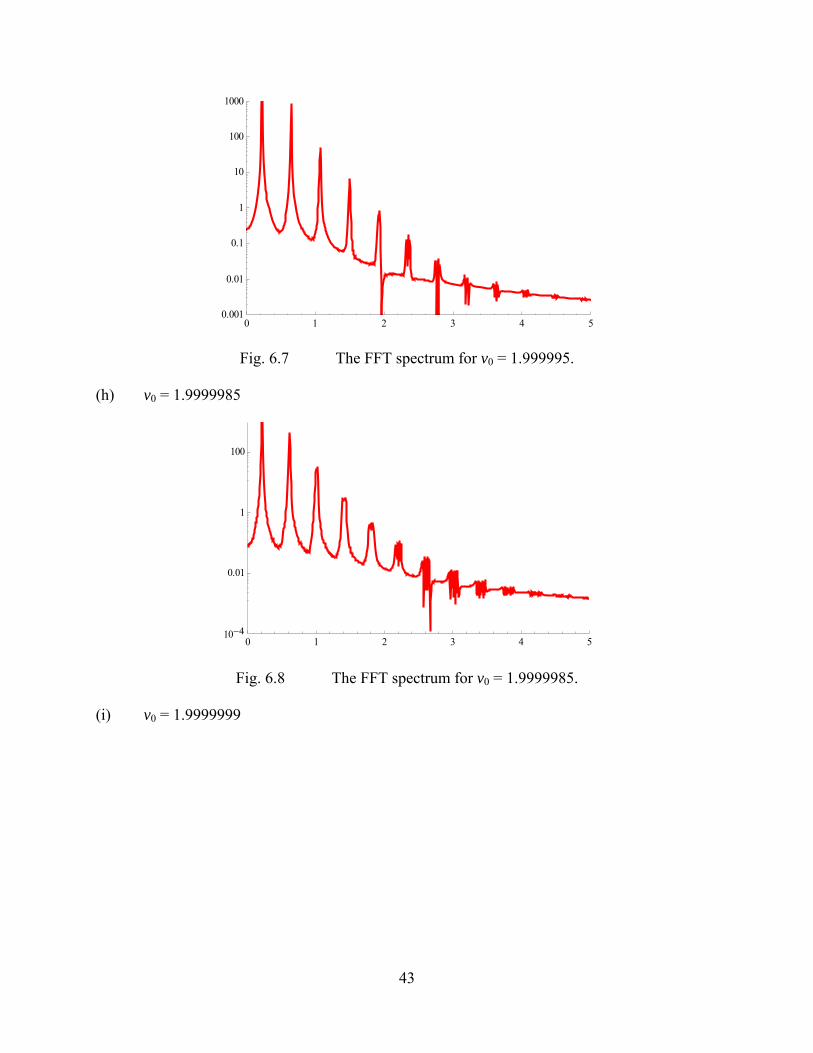
Fig. 6.7 The FFT spectrum for v0 = 1.999995. (h) v0 = 1.9999985

Fig. 6.8 The FFT spectrum for v0 = 1.9999985. (i) v0 = 1.9999999

0 1 2 3 4 50.001

0.01

0.1

1

10

100

1000

0 1 2 3 4 510-4

0.01

1

100

44

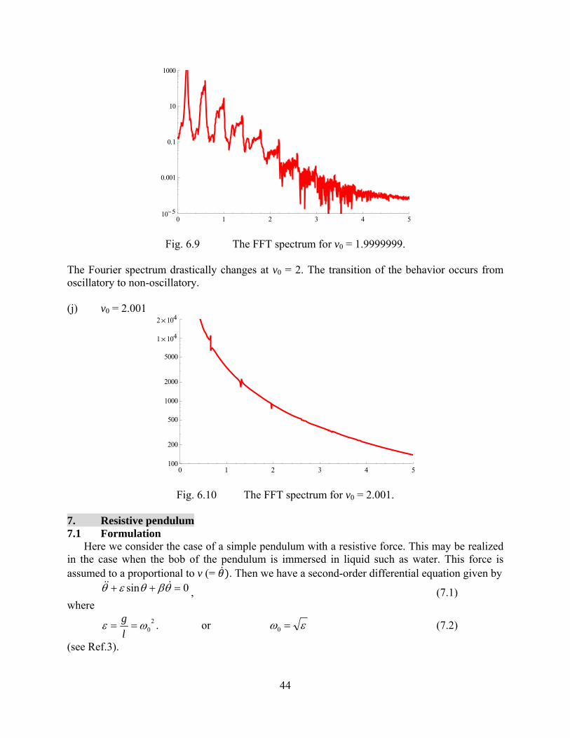
Fig. 6.9 The FFT spectrum for v0 = 1.9999999. The Fourier spectrum drastically changes at v0 = 2. The transition of the behavior occurs from oscillatory to non-oscillatory. (j) v0 = 2.001

Fig. 6.10 The FFT spectrum for v0 = 2.001. 7. Resistive pendulum 7.1 Formulation

Here we consider the case of a simple pendulum with a resistive force. This may be realized in the case when the bob of the pendulum is immersed in liquid such as water. This force is assumed to a proportional to v (= . Then we have a second-order differential equation given by

0sin =++ θβθεθ &&&, (7.1)

where 2

0ωε ==lg . or εω =0 (7.2)

(see Ref.3).

0 1 2 3 4 510-5

0.001

0.1

10

1000

0 1 2 3 4 5

1μ 104

2μ 104

100

200

500

1000

2000

5000

45

Here we assume that β is a very small positive value. The above differential equation is equivalent to a pair of the first-order differential equations, which are given by

vvv

βθεθ

−−==

sin&

&, (7.3)

or

vvv

ddv )sin( βθε

θθ+

−== && . (7.4)

In Eq.(7.4), both the numerator and the denominator of the right-hand side become zero when v = 0 and θ = nπ. This point in the trajectory in the v vs θ plane is called a singular point. In order to study the detail of the trajectory near the singular point, we introduce a new variable φ, which is defined by

φπθ += n . (7.5) Then we get

vvnvv

n βεφβφπε

φ

−−≈−+−=

=+1)1()sin(&

&, (7.6)

or the second-order differential equation 0)1( =−++ εφφβφ n&&&

. (7.7) When n = even, this equation is the same as one of simple harmonics with viscous damping;

0=++ εφφβφ &&&, (7.8)

where 2√ . Thus the points (v = 0 ,θ = 0, 2π. 4π,…) are stable spiral points. For n = odd, the situation is rather different,

0=−+ εφφβφ &&&. (7.9)

When teλφ ∝ , the value of λ satisfies the quadratic equation given by 02 =−+ εβλλ . (7.10)

The roots of this equation are real. One root is a real positive and the other is a real negative. In this case the points (v = 0 ,θ = π, 3π. 5π,…) are saddle points. 7.2 Numerical calculation using Mathematica 7.2.1 Time dependence of θ

We calculate the time dependence of θ numerically. The Mathematica program with a NDSolve command, is used to solve the differential equations given by

)()(sin)()()(

tvttvtvt

βθεθ

−−==

&

&, (7.11)

with an initial conditions,

0

0

)0()0(

θθ == vv

. (7.12)

For simplicity, we choose ε = 1 and θ0 = 0. Figure 7.1 shows the plot of θ vs t for v0 = 2.3, where β is changed as a parameter (0.01 β 0.16). Note that for β = 0, the pendulum continues to rotate around the pivot point for v0 > 2. For finite values of β (see Fig.7.1), however, the rotation angle θ increases with increasing t, and after a characteristic time depending on β, it

46

starts to oscillate around a fixed value (2nπ) with integer n and tends to reduce to the value 2nπ. The value of n is strongly dependent on the value of β; n = 0 for β = 0.16, n = 1 for β = 0.12 and 0.08, n = 1 for β = 0.04, n = 3 for β = 0.02, n = 4 for β = 0.018 and 0.016, n = 5 for β = 0.014, n = 6 for β = 0.012, and n = 7 for β = 0.010.

Figure 7.2 shows the plot of v vs t for v0 = 2.3, where β is changed as a parameter (0.04 β 0.16). The angular velocity v oscillates around v = 0 and tends to decay after sufficient long times. In other words, the average angular velocity (or the terminal angular velocity) is equal to zero, for any β (except for β = 0).

Fig.7.1 θ vs t for ε = 1. v0 = 2.3. β is changed as a parameter. β = 0.010 (red), 0.012, 0.014, 0.016, 0.018, 0.020, 0.04, 0.08, 0.12, and 0.16 (blue).

Fig.7.2 v vs t for ε = 1. v0 = 2.3. β is changed as a parameter. β = 0.04 (red), 0.08 (light green), 0.12 (light blue), and 0.16 (dark blue).

7.2.2 Trajectories in the phase space of v vs θ.

Figure 7.3 shows the trajectories in the phase space of v vs θ, where ε = 1, v0 = 2.3, and β is changed as a parameter. The spiral (stable) point are at θ = 2nπ and v = 0, where n is an integer

10 20 30 40 50 60 70 80 90 100t HsL

2 p

4 p

6 p

8 p

10 p

12 p

14 p

q

50 100 150t HsL

-1

1

2

v

47

and the saddle points are at θ = (2n+1)π and v = 0. Each trajectories for finite β (β 0 converges to the spiral points. The spiral points become far away from the origin with decreasing β. The terminal angular velocity v (the angular velocity at sufficiently long times) is equal to zero except for the case of β = 0.

Fig.7.3 Trajectories in the phase space of v (= vs θ for ε = 1 and v0 = 2.3. β is changed as a parameter. β = 0, (red), 0.02, 0.04, 0.06, 0.08, 0.10, 0.12, 0.14, 0.16, 0.18, and 0.20 (green).

8. Simple rigid pendulum and Josephson junctions 8.1 Formulation

Finally we consider the motion of the pendulum with an applied torque T around the pivot point P.

Fig.8.1 Simple pendulum with an applied torque. The equation of motion for the pendulum is given by

θηθθ &&& −−= sinmglTI , (8.1)

p 2 p 3 p 4 p 5 p 6 p 7 pq

-2-1

12

v

48

where T is an external torque, I is a moment of inertia around the pivot P and the third term of the right-hand side is a viscosity of air. Since , this equation can be rewritten as

θεθβθτ sin++= &&&, (8.2)

where

2mlηβ =

, and 2ml

T=τ

. (8.3) For simplicity we assume that ε = 1. 8.2 Numerical calculation for the simple case 8.2.1 The trajectory in the phase space v vs θ (β = 0.16 and v0 = 0.2)

The trajectory changes from the spiral orbits (small τ) to the open orbits (large τ) around τ = 0.6 – 0.8. The stable point of the spiral orbits is moved from the origin to an equilibrium point (= θs) on the positive θ axis (v = 0). The value of θs is related to τ as

sθτ sin= , (8.4) for τ≤0.6. This relation is valid at least for small β and small v0.

Fig.8.2 The trajectory in the phase space of v vs θ. β = 0.16 and v0 = 0.2. τ is changed as a parameter. τ = 0 (red), 0.2 (light blue), 0.4, 0.6 (dark blue), and 0.8 (yellow).

8.2.2 The trajectory in the phase space v vs θ (β = 0.16. v0 = 1.98) for τ = 0.19 – 0.25.

The trajectory changes from the spiral orbits (small τ) to the open orbits (large τ) around τ = 0.21. The stable point of the spiral orbits is moved from the origin to an equilibrium point (= θs)

p4

p2

q

-0.5

0.5

1.v

49

on the positive θ axis (v = 0). On the other hand, the value of v on the open orbit oscillates with increasing θ and reaches an equilibrium value v0 (= 1.98 here). Figure 8.4 shows the time dependence of v, which drastically changes around τ = 0.21. For τ = 0.20, v oscillate around v = 0 with time t, while for τ>0.22, v oscillates around a finite value of v (not equal to zero) with time t,

Fig.8.3 Trajectories in the phase space for of v vs θ. τ = 0.19 (red), 0.20, 0.21 (blue), 0.22, 0.23, and 0.24 (purple).

Fig.8.4 The time dependence of v for τ = 0.19, 0.20, 0.21, 0.22, 0.23, and 0.24. 8.2. β = 0.16. τ = -0.01 – 0.40 (the separation Δτ = 0.01)

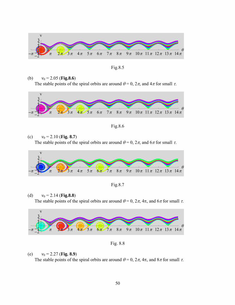
Through the computer simulation we find some peculiar behavior in the trajectories in the phase space, where β = 0.16 and ε = 1. For each v0 (= 2.01 – 3.15), the value of τ is changed as a parameter: typically τ = 0.01 – 0.40 with Δτ = 0.01. The trajectory changes from the spiral orbit for small τ to the open orbit for large τ. (a) v0 = 2.01 (Fig.8.5)

The stable points of the spiral orbits are around θ = 0 and 2π for small τ.

-p p 2 p 3 p 4 pq

-2

-1

1

2

3v

50 100 150t

-2

-1

0

1

2

v

50

Fig.8.5 (b) v0 = 2.05 (Fig.8.6)

The stable points of the spiral orbits are around θ = 0, 2π, and 4π for small τ.

Fig.8.6 (c) v0 = 2.10 (Fig. 8.7)

The stable points of the spiral orbits are around θ = 0, 2π, and 6π for small τ.

Fig.8.7 (d) v0 = 2.14 (Fig.8.8)

The stable points of the spiral orbits are around θ = 0, 2π, 4π, and 6π for small τ.

Fig. 8.8 (e) v0 = 2.27 (Fig. 8.9)

The stable points of the spiral orbits are around θ = 0, 2π, 4π, and 8π for small τ.

-p p 2 p 3 p 4 p 5 p 6 p 7 p 8 p 9 p 10 p 11 p 12 p 13 p 14 pq

-2-1

123

v

-p p 2 p 3 p 4 p 5 p 6 p 7 p 8 p 9 p 10 p 11 p 12 p 13 p 14 pq

-2-1

123

v

-p p 2 p 3 p 4 p 5 p 6 p 7 p 8 p 9 p 10 p 11 p 12 p 13 p 14 pq

-2-1

123

v

-p p 2 p 3 p 4 p 5 p 6 p 7 p 8 p 9 p 10 p 11 p 12 p 13 p 14 pq

-2-1

123

v

51

Fig. 8.9 (e) v0 = 2.40 (Fig. 8.10)

The stable points of the spiral orbits are around θ = 0, 2π, 4π, 6π, and 8π for small τ.

Fig. 8.10 (f) v0 = 2.60 (Fig. 8.11)

The stable points of the spiral orbits are around θ = 0, 2π, 4π, 6π, and 10π.

Fig.8 11 (g) v0 = 2.80 (Fig. 8.12)

The stable points of the spiral orbits are around θ = 0, 2π, 4π, 6π, 8π and 10π.

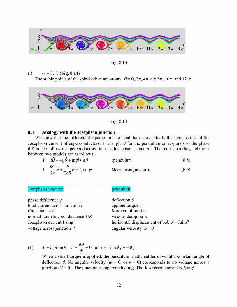
Fig. 8.12 (h) v0 = 2.95 (Fig. 8.13)

The stable points of the spiral orbits are around θ = 0, 2π, 4π, 6π, 8π and 12π.

-p p 2 p 3 p 4 p 5 p 6 p 7 p 8 p 9 p 10 p 11 p 12 p 13 p 14 pq

-2-1

123

v

-p p 2 p 3 p 4 p 5 p 6 p 7 p 8 p 9 p 10 p 11 p 12 p 13 p 14 pq

-2-1

123

v

-p p 2 p 3 p 4 p 5 p 6 p 7 p 8 p 9 p 10 p 11 p 12 p 13 p 14 pq

-2-1

123

v

-p p 2 p 3 p 4 p 5 p 6 p 7 p 8 p 9 p 10 p 11 p 12 p 13 p 14 pq

-2-1

123

v

52

Fig. 8.13 (i) v0 = 3.15 (Fig. 8.14)

The stable points of the spiral orbits are around θ = 0, 2π, 4π, 6π, 8π, 10π, and 12 π.

Fig. 8.14 8.3 Analogy with the Josephson junction

We show that the differential equation of the pendulum is essentially the same as that of the Josephson current of superconductors. The angle θ for the pendulum corresponds to the phase difference of two superconductors in the Josephson junction. The corresponding relations between two models are as follows.

θθηθ sinmglIT +++= &&& (pendulum). (8.5)

φφφ sin22 cIeRe

CI ++= &h&&h (Josephson juncton). (8.6)

_______________________________________________________________________ Josephson junction pendulum phase difference φ deflection θ total current across junction I applied torque T Capacitance C Moment of inertia normal tunneling conductance 1/R viscous damping η Josephson current Icsinφ horizontal displacement of bob θsinlx = voltage across junction V angular velocity θω &= _______________________________________________________________________

(1) θsinmglT = , 0==dtdθω (or θετ sin= , 0=v )

When a small torque is applied, the pendulum finally settles down at a constant angle of deflection θ. No angular velocity (ω = 0, or v = 0) corresponds to no voltage across a junction (V = 0). The junction is superconducting. The Josephson current is Icsinφ.

-p p 2 p 3 p 4 p 5 p 6 p 7 p 8 p 9 p 10 p 11 p 12 p 13 p 14 pq

-2-1

123

v

-p p 2 p 3 p 4 p 5 p 6 p 7 p 8 p 9 p 10 p 11 p 12 p 13 p 14 pq

-2-1

123

v

53

(2) If the torque is gradually increased, the pendulum deflects to a greater but steady angle. We can pass more current through a junction without any voltage appearing.

(3) Critical torque Tc = mgl (or τc = ε). This is the torque which deflects the pendulum through a right angle so that it is horizontal.

(4) For T>Tc (or τ >ε), the pendulum cannot remain at rest but rotates continuously. As the pendulum rotates, the horizontal deflection x oscillates. The angular velocity is always in the same direction. This corresponds to the case of I>Ic and V≠0. A DC voltage will appear across the junction if the current passed through it exceeds a critical value.

The detail of the Josephson junction and DC SQUID will be found in the Lecture Note on the

Solid State Physics (M. Suzuki and I.S. Suzuki). All the calculations are made using the NDSolve command in the Mathematica. 9. CONCLUSION

The physics of a simple pendulum for large angles is much more complicated than that for small angle because of the nonlinearity of the system. The time dependence of the angle can be exactly described by a Jacobi elliptic function. The numerical calculation can be also used to solve the nonlinear differential equation with appropriate initial conditions. As is expected, the results of numerical calculation are in excellent agreement with the exact solutions from the theory without any approximation. The numerical method is not so useful for a simple pendulum since the exact solution is expressed by a Jacobi elliptic function. This method becomes very powerful when the perturbation effect becomes significant in a system such as a resistive pendulum with an external torque. In this note, we show that the trajectories in the phase space in such a system are strongly dependent on the damping factor, the initial velocity, and the external torque because of the nonlinearity of the system. The nature of nonlinearity for the Josephson junction is essentially the same as that of the resistive pendulum with an external torque. The study on the physics of the pendulum is a key to understand the nature of nonlinear dynamics in the general systems.

Finally we stress that the book by Toda is very useful for us to understand the essential points of the vibration. Unfortunately, the book was written in Japanese. As far as we know no translation of the book has been made from Japanese to English. If the book is translated from Japanese to English, many readers over the world will think that the book is excellent. REFERENCES 1. A.B. Pippard, The Physics of Vibrartion 1 (Cambridge University Press 1978). 2. M. Toda, Theory of Oscillation (Shokabo, Tokyo 1975) [in Japanese]. 3. G.L. Baker and J.A. Blackburn, The Pendulum, a case study in physics (Oxford

University Press 2005, New York). 4. M. Suzuki and I.S. Suzuki, Lecture Note on Solid State Physics Josephson junction and

DC SQUID; http://www.binghamton.edu/physics/Sei_Suzuki/suzuki.html 5. Pendulum, Wikipedia, http://en.wikipedia.org/wiki/Pendulum APPENDIX A. Elliptic Integral of the First Kind

54

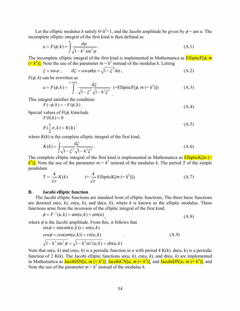
Let the elliptic modulus k satisfy 0<k2<1, and the Jacobi amplitude be given by φ = am u. The incomplete elliptic integral of the first kind is then defined as

∫ −==

φ

ϕϕφ

022 sin1

),(kdkFu . (A.1)

The incomplete elliptic integral of the first kind is implemented in Mathematica as EllipticF[φ, m (= k2)]. Note the use of the parameter m = k2 instead of the modulus k. Letting

ϕξ sin= , ϕξϕϕξ ddd 21cos −== , (A.2) F(φ, k) can be rewritten as

∫=

−−==

φ

ξξξφ

sin

0222 11

),(z

kdkFu

. (=EllipticF[φ, m (= k2)]) (A.3)

This integral satisfies the condition ),(),( kFkF φφ −=− . (A.4)

Special values of F(φ, k)include

)(),21(

0),0(

kKkF

kF

=

=

π, (A.5)

where K(k) is the complete elliptic integral of the first kind,

∫ −−=

1

0222 11

)(ξξ

ξk

dkK . (A.6)

The complete elliptic integral of the first kind is implemented in Mathematica as EllipticK[m (= k2)]. Note the use of the parameter m = k2 instead of the modulus k. The period T of the simple pendulum

)(4 kKTε

= (=ε4 EllipticK[m (= k2)]). (A.7)

B. Jacobi elliptic function

The Jacobi elliptic functions are standard form of elliptic functions, The three basic functions are denoted sn(u, k), cn(u, k), and dn(u, k), where k is known as the elliptic modulus. These functions arise from the inversion of the elliptic integral of the first kind,

)(),(),(1 uamkuamkuF === −φ , (A.8)

where φ is the Jacobi amplitude. From this, it follows that

),(),(1sin1

),()),(cos(cos),()),(sin(sin

2222 kudnkusnkk

kucnkuamkusnkuam

=−=−

====

φ

φφ

. (A.9)

Note that sn(u,k) and cn(u, k) is a periodic function in u with period 4 K(k). dn(u, k) is a periodic function of 2 K(k). The Jacobi elliptic functions sn(u, k), cn(u, k), and dn(u, k) are implemented in Mathematica as JacobiSN[u, m (= k2)], JacobiCN[u, m (= k2)], and JacobiDN[u, m (= k2)], and Note the use of the parameter m = k2 instead of the modulus k.

55

Fig.A1 Plot of sn(u, m) as a function of u, where m is changed as a parameter. m = 0 (red), 0.2, 0.4 0.6, 0.8 (blue), and 1.0 (purple).

C Typical Mathematical program C.1 Commands of mathematica

We use the following Mathematica commands in the present calculations. Fourier

Fourier[list] finds the discrete Fourier transform of a list of complex numbers. NDSolve

NDSolve[eqns, y, {x, xmin, xmax}] finds a numerical solution to the ordinary differential equations eqns for the function y with the independent variable x in the range xmin to xmax.

EllipticK[m (= k2)]

EllipticK[m = k2] gives the complete elliptic integral of the first kind )( mkK = . JacobiSN[u, m (= k2)] and JacobiCN[u, m (= k2)]

JacobiSN[u, m], JacobiCN[u, m], etc. give the Jacobi elliptic functions,

),( mkusn = and ),( mkucn = . ContourPlot

ContourPlot[f == g, {x, xmin, xmax}, {y, ymin, ymax} ] plots contour lines for which f = g, in the x-y plane

Graphics

Graphics[primitives,options] represents a two-dimensional graphical image. ParametricPlot

ParametricPlot[{fx(u), fy(u)}, {u, umin, umax}] generates a parametric plot of a curve with x and y coordinates and fx(u) and fy(u)} are a function of u.

56

C.2 FFT analysis using Fourier (Mathematica program) (Section 2.4 and Chapter 6)

Fig.A2 v0 = 1.92. C.3 Geometry from Graphics (Chapter 4)

FFT analysis of the wave form for Simple Pendulum

We analyze the Fourier conmonent by using FFT (Mathematica , Fourier).

1. We choose the N (= 2n) data, typically the data between 0 and T (=tmax).2. The minimum time division is D= T

N, which corresponds to the maximum wmax = 2 p

D= 2 p

TN

3. Th Fourier spectrum is plotted as a function of the channel numer multiplied by 2 pT

.

In[1]:= Clear@"Global`∗"D

In[2]:= G1@t_D := 2 ArcSinAk JacobiSNAt, k2EE ê. k →v0

2

In[3]:= pentime@8θ0_, v1_<, ε_, tmax_, N1_D :=

ModuleB8numtable<,

numtable = TableB8t, G1@tD ê. v0 → v1<, :t, 0, tmax,tmax

N1>FF

In[4]:= eq1 = pentime@80, 1.92<, 1, 1600, 32 768D; d1 = Dimensions@eq1D@@1DD;list1 = Table@eq1@@i, 2DD, 8i, 1, d1 − 1<D; list2 = Fourier@list1D êê Chop;

list3 = TableB: 2 π

1600n, Abs@list2@@nDDD2>, 8n, 0, 32 768<F;

ListLogPlot@list3, Joined → True,PlotRange → 880, 5<, 80.0001, 100 000<<, PlotStyle → 8Thick, Red<,PlotLabel → 1.92D

Out[4]=

0 1 2 3 4 510-4

0.01

1

100

104

1.92

57

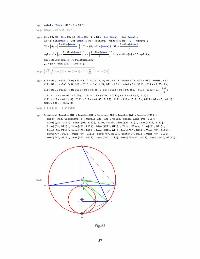
Fig.A3

In[1]:= rule1 = 8θmax → 80 °, θ → 50 °<Out[1]= 8θmax → 80 °, θ → 50 °<

In[2]:= O1 = 80, 0<; E1 = 80, 1<; A1 = 80, −1<; B1 = 8Sin@θmaxD, −Cos@θmaxD<;B2 = 8−Sin@θmaxD, −Cos@θmaxD<; P1 = 8Sin@θD, −Cos@θD<; N1 = 80, − Cos@θD<;

O2 = :0, −1 + Cos@θmaxD

2>; D1 = 80, −Cos@θmaxD<; R2 =

1 − Cos@θmaxD2

;

eq1 = x2 + y +1 + Cos@θmaxD

2

2==

1 − Cos@θmaxD2

2ê. y → −Cos@θD êê Simplify;

eq2 = Solve@eq1, xD êê FullSimplify;Q1 = 8x ê. eq2@@2DD, −Cos@θD<

Out[2]= : 2 HCos@θD − Cos@θmaxDL SinBθ2F2

, −Cos@θD>

In[3]:= B11 = B1 ê. rule1 êê N; B21 = B2 ê. rule1 êê N; P11 = P1 ê. rule1 êê N; O21 = O2 ê. rule1 êê N;N11 = N1 ê. rule1 êê N; Q11 = Q1 ê. rule1 êê N; R21 = R2 ê. rule1 êê N; B111 = B11 + 80.05, 0<;

D11 = D1 ê. rule1 êê N; O111 = O1 + 80.05, 0.05<; O112 = O1 + 80.055, −0.1<; O113 = O1 +B11

5;

D111 = D11 + 8−0.05, −0.05<; D112 = D11 + 80.04, −0.1<; E111 = E1 + 80, 0.1<;N111 = N11 + 8−0.1, 0<; Q111 = Q11 + 8−0.05, 0.05<; P111 = P11 + 80.1, 0<; A111 = A1 + 80, −0.1<;B211 = B21 + 8−0.1, 0<

Out[3]= 8−1.08481, −0.173648<

In[4]:= Graphics@8Locator@E1D, Locator@O1D, Locator@O21D, Locator@A1D, Locator@D11D,Thick, Red, Circle@O1, 1D, Circle@O21, R21D, Thick, Green, Line@8O1, P11<D,Line@8Q11, D11<D, Line@8O1, B11<D, Blue, Thick, Line@8A1, E1<D, Line@8B21, B11<D,Line@8O1, B21<D, Line@8E1, P11<D, Line@8P11, N11<D, Thin, Black, Line@8E1, B11<D,Line@8A1, P11<D, Line@8A1, B11<D, Line@8Q11, A1<D, Text@"E" , E111D, Text@"B", B111D,Text@"O" , O111D, Text@"D", D111D, Text@"N", N111D, Text@"Q", Q111D, Text@"P", P111D,Text@"A", A111D, Text@"φ", D112D, Text@"θ", O112D, Text@"θmax", O113D, Text@"B'", B211D<D

Out[4]=

58

C.4 Numerical method of solving differential equation (NDSolve) (Chapters 5, 7, and 8)

Initial conditionq(t=0)=0, q'(t=0)=v0The total energy E is conserved. E= 1

2v02. The maximum of the potential energy is 2e.

e=w02. The character of the motion drastically changes when E is larger than 2e. In other words, The critical value of v0 is v0=2 e .

phase@8θ0_, v0_<, ω0_, tmax_, opts__D :=

ModuleA8numso1, numgraph<,

numso1 =

NDSolveA9 ω02 Sin@θ@tDD + v'@tD 0, v@tD == θ'@tD,

θ@0D θ0, v@0D v0=, 8θ@tD, v@tD<, 8t, 0, tmax<E êê Flatten;

numgraph = Plot@Evaluate@θ@tD ê. numso1D, 8t, 0, tmax<,opts, DisplayFunction → IdentityDE

For simplicity we assume that w0 = 1 (e=1). The critical value of v0 is 2 in this case.

(a) v0 = 1.999992, 1.999993, 1.999994, 1.999995, 1.999996, 1.999997, 1.999998, 1.999999

phlist =

phaseB80, <, 1.0, 100,

PlotStyle → 8Thick, Hue@100 000 H − 1.999992LD<,AxesLabel → 8"t", "θ"<, Prolog → AbsoluteThickness@2D,Background → GrayLevel@0.5D, PlotRange → All,

Ticks → : Range@0, 100, 10D, π RangeB−3

2,

3

2,

1

2F>,

DisplayFunction → IdentityF & ê@

Range@1.999992, 1.999999, 0.000001D;Show@phlist, DisplayFunction → $DisplayFunctionD

10 20 30 40 50 60 70 80 90 100t

-p

- p2

p2

p

q

59

Fig. A4

C.5 ContourPlot (Section 3.1)

Fig.A5 C.6 ParametricPlot: Trajectories in the phase space (Section 8.2)

In[1]:= G1@v0_D := SinB θ

2F == JacobiSNBt

κ, κ2F ê. κ →

2

v0

In[2]:= f2 = ContourPlot@Evaluate@G1@2.1DD, 8t, 0, 30<, 8θ, 0, 20 π<,ContourStyle → 8Thick, Red<, Background → LightGray,PlotPoints → 70, PlotLabel → 2.1D

Out[2]=

0 5 10 15 20 25 300

10

20

30

40

50

60

2.1

In[3]:=

60

Fig.A6

In[1]:= Clear@"Global`∗"D

In[2]:= phase@8θ0_, τ_<, 8β_, v0_<, tmax_, opts__D :=

Module@8numso1, numgraph<,numso1 =

NDSolve@8 v '@tD + β v@tD+ Sin@θ@tDD τ, θ '@tD v@tD, θ@0D θ0,v@0D v0<, 8v@tD, θ@tD<, 8t, 0, tmax <D êê Flatten;

numgraph = ParametricPlot@8Evaluate@θ@tD ê. numso1D, Evaluate@v@tD ê. numso1D<,8t, 0, tmax <, opts, DisplayFunction → IdentityDD

In[3]:= phlist =

phase@80, <, 80.16, 2.1<, 100, PlotStyle → 8Thick, Hue@8 H − 0.05LD<,AxesLabel → 8"θ", "v"<, Background → LightGray,PlotRange → 88− π, 14 π<, 8−2, 3<<,Ticks → 8 π Range@−10, 14D, Range@−2, 4D<,DisplayFunction → IdentityD & ê@ Range@0.01, 0.35, 0.01D;

Show@phlist, DisplayFunction → $DisplayFunctionD

Out[3]=

-p p 2 p 3 p 4 p 5 p 6 p 7 p 8 p 9 p 10 p 11 p 12 p 13 p 14 pq

-2

123v