0

Tomsk Polytechnic University

Antonov V. M., Pichugin V. F., Pivovarov Yu. L.

PHYSICS II Textbook

Electricity and Magnetism. Electromagnetic Oscillations and

Waves

Tomsk 2002

1

UDC 53 (076)

Antonov V. M., Pichugin V. F., Pivovarov Yu. L. PHYSICS II. Electricity

and Magnetism. Electromagnetic Oscillations and Waves. Textbook.

Tomsk: TPU, 2002, 93 pp.

This textbook is the second part of the general course in physics for

technical universities. It includes Electricity and Magnetism, Oscillations

and Waves. The main theoretical concepts are formulated in logical

fashion. There are many examples and practice problems to be solved. This

textbook has been approved by the Department of Theoretical and

Experimental Physics and the Department of General Physics of TPU.

Reviewed by: V.Ya. Epp, Professor of Department Physics and

Mathematics, TSPU, D.Sc.

2

Preface 3

1. 1 Electric Field in a Vacuum 2

1.1 Electric charge 2

1.2 Coulomb’s law 3

1.3 Electric Field Strength 3

1.4 Gauss’ Theorem

4

1.5 Calculating fields with the aid of Gauss’ theorem 5

1.6 Potential 7

1.7 Relations between the electric field strength and potential 8

1.8 Equipotential Surfaces and Strength Lines 9

1.9 Capacitance 10

1.10 Interaction Energy of a System of Charges 12

1.11 Energy of a Charged Conductor 12

1.12Energy of a Charged Capacitor 12

1.13 Examples 13

2. Electric Field in Dielectrics 21

2.1. Dipole Electric Moment 21

2.2. Polar and Non-polar Molecules 22

2.3 Polarization of Dielectrics 22

2.4 Space and Surface Bound Charges 23

25 Electric Displacement Vector 25

2.6 Examples of Calculating the Field in Dielectrics 26

2.7 Conditions at the Interface Between Two Dielectrics 29

2.8 Forces Acting on a Charge in a Dielectric 31

Examples 32

3. Steady Electric Current 37

3.1. Electric Current 37

3.2. Continuity Equation 38

3.3 Electromotive Force 39

3.4. Ohm’s Law. Resistance of Conductors 40

3.5. Ohm’s Law for an Inhomogeneous Circuit Section 41

3.6 Kirchhoff’s Rules 42

3.7 Power of a Current 43

3.8 The Joule-Lenz Law 43

Examples 44

4. 4. Magnetic Field 46

4.1. Biot-Savart’s law. Ampere’s law 46

4.2 The Flux and Circulation of Magnetic Field 34

4.3 Lorentz’s force. Hall’s effect 58

4.4 Electromagnetic induction 63

3

Problems to Chapter 4 (Magnetic field) 65

5. Magnetic field in matter 66

5.1 Magnetic moments of atoms 66

5.2 Magnetic properties of matter 69

5.3 Classification of Magnetic Materials (Substances) 70

6. Maxwell’s Equations .72

6.1 Maxwell’s Equations in an Integral Form 72

6.2 . Maxwell’s Equations in the Differential Form 75

7. Electromagnetic oscillations and waves 77

7.1. Electromagnetic oscillations 77

7.2 7.2. Electromagnetic Waves 83

4

PREFACE

This textbook is a second part of course in introductory physics for students

mastering science or engineering. The main objective of this part is electromagnetism,

which involves the theory of electricity, magnetism, and electromagnetic fields.

The mathematical background of the student taking this course should include

one or two semesters of calculus. A large number of examples of varying difficulty are

presented as an aid in understanding concepts. In many cases, these examples serve as

models for solving another problems.

Electricity and Magnetism

2. Electric Field in a Vacuum 2.1 Electric charge

Electrostatics is a science dealing with the interaction of electric charges at rest.

The motion at velocities v<<c may also be taken into consideration.

In nature there are two kinds of electric charges: positive and negative. These

definitions have been established historically. In our “common” world, the electric

charge of a body is caused either by excess of deficiency of electrons or protons – the

main particles of which atoms are composed, (the third fundamental particle – neutron

has no electric charge). The electron carries the negative charge –e, the proton carries

the positive charge +e. SI unit of e = 1.610-19

Coulomb. One coulomb is a charge,

passing through the conductor’s cross-section during the unit time (1 sec) when the

current strength equals 1A.

Electrons, protons and neutrons are the “bricks” of which the atoms and

molecules of any substance are built , therefore all bodies contain electric charges. The

charge q of a body is formed by a plurality of elementary charges, i.e.

Neq (1.1)

An elementary charge is so small that macroscopic charges may be considered to have

continuously changing magnitudes.

The magnitude of a charge in different inertial frames is known to be the same;

thus, an electric charge is a relativistic invariant.

Electric charges can vanish and appear again. Two elementary charges of

opposite signs always appear or vanish simultaneously. For example, an electron and

positron meeting each other annihilate themselves giving birth to two or more gamma-

photons: e-+e

+2. And vice versa, a gamma-photon getting into the field of an atomic

nucleus transforms into a pair of particles (an electron and a positron), i.e.: e-+e

+.

Thus, the total charge of an electrically isolated system (no charged particles can

penetrate through the surface confining it) does not change. This statement forms the

law of electric charge conservation. It must be noted that the law is associated with the

relativistic invariance of a charge. Indeed, if the magnitude of a charge depended on its

velocity, then by bringing charges of one sign into motion we would change the total

charge of the relevant isolated system.

5

2.2 Coulomb’s law

The law describing the interaction between point charges was established

experimentally in 1785 by Charles A. De Coulomb. A point charge is defined as a

charged body whose dimensions may be disregarded in comparison with the distances

from this body to other bodies carrying electric charges. Coulomb’s law can be

formulated as follows: the force of interaction between two stationary point charges is

proportional to the magnitude of each of them and inversely proportional to the square

of the distance between them; the direction of the force coincides with that of straight

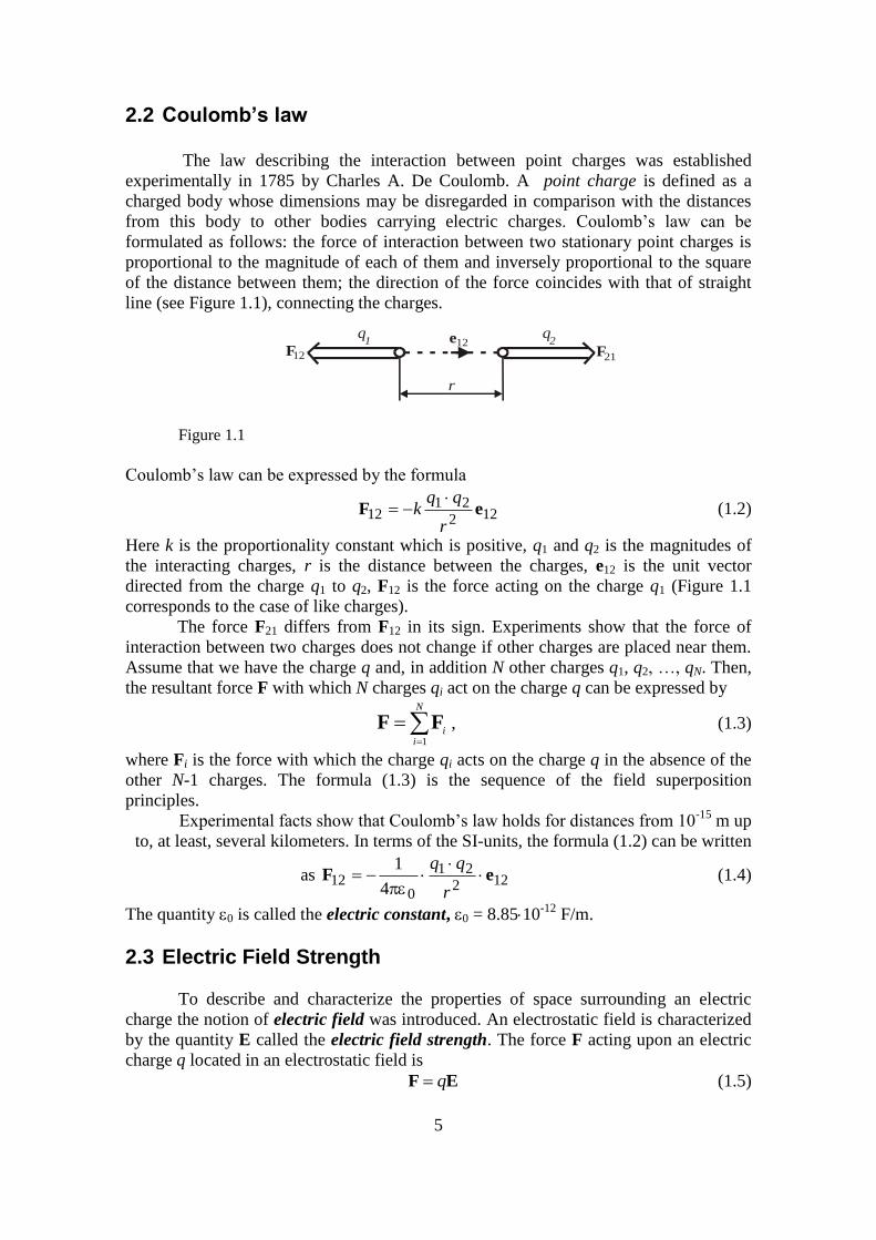
line (see Figure 1.1), connecting the charges.

Figure 1.1

Coulomb’s law can be expressed by the formula

122

2112 eF

r

qqk

(1.2)

Here k is the proportionality constant which is positive, q1 and q2 is the magnitudes of

the interacting charges, r is the distance between the charges, e12 is the unit vector

directed from the charge q1 to q2, F12 is the force acting on the charge q1 (Figure 1.1

corresponds to the case of like charges).

The force F21 differs from F12 in its sign. Experiments show that the force of

interaction between two charges does not change if other charges are placed near them.

Assume that we have the charge q and, in addition N other charges q1, q2, …, qN. Then,

the resultant force F with which N charges qi act on the charge q can be expressed by

N

ii

1

FF , (1.3)

where Fi is the force with which the charge qi acts on the charge q in the absence of the

other N-1 charges. The formula (1.3) is the sequence of the field superposition

principles.

Experimental facts show that Coulomb’s law holds for distances from 10-15

m up

to, at least, several kilometers. In terms of the SI-units, the formula (1.2) can be written

as 122

21

012

4

1eF

r

qq (1.4)

The quantity 0 is called the electric constant, 0 = 8.8510-12

F/m.

2.3 Electric Field Strength

To describe and characterize the properties of space surrounding an electric

charge the notion of electric field was introduced. An electrostatic field is characterized

by the quantity E called the electric field strength. The force F acting upon an electric

charge q located in an electrostatic field is

EF q (1.5)

q q

r

e12F F12 21

1 2

6

Comparing (1.5) and (1.4) we come to a conclusion that the electric field strength

produced by a point charge q at a distance r is equal (absolute magnitude) to

204 r

qE

(1.6)

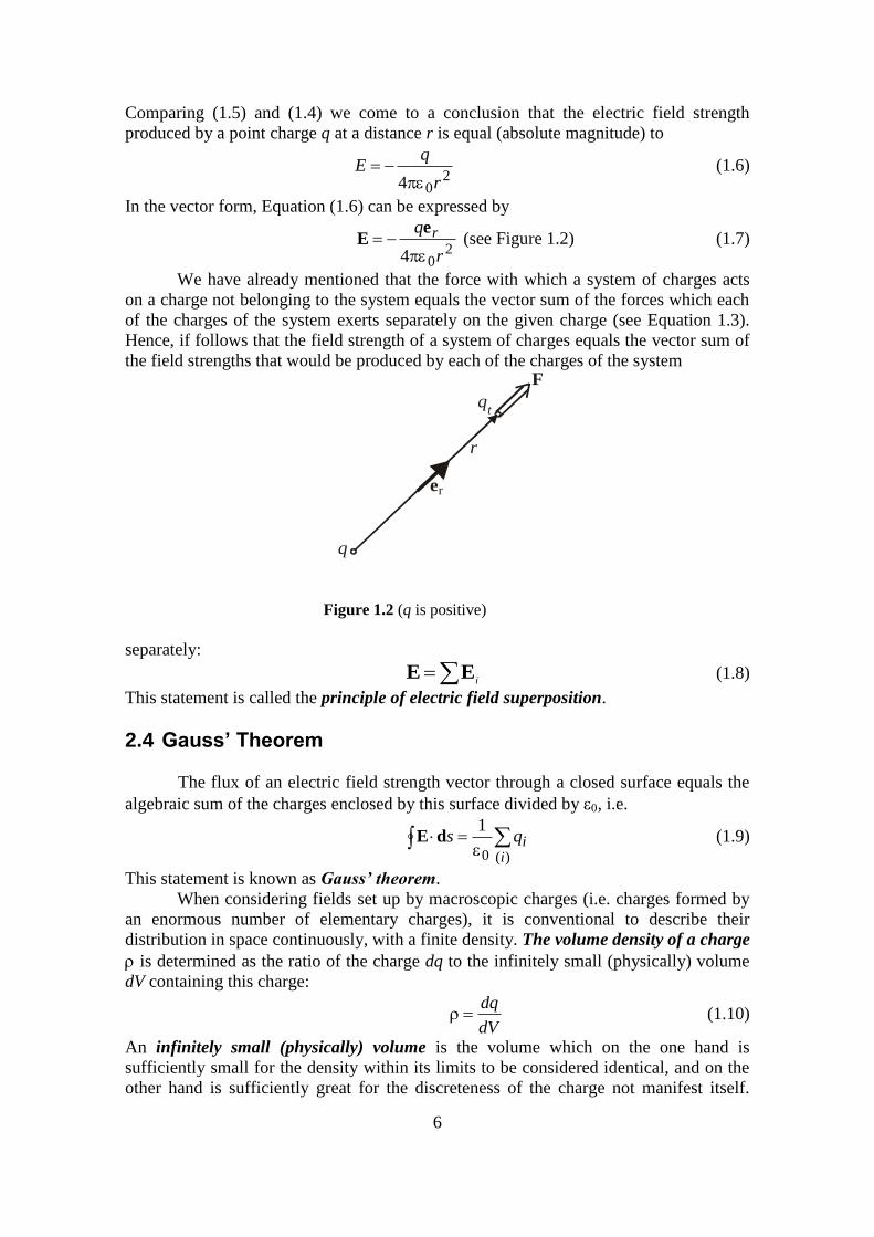
In the vector form, Equation (1.6) can be expressed by

204 r

q r

eE (see Figure 1.2) (1.7)

We have already mentioned that the force with which a system of charges acts

on a charge not belonging to the system equals the vector sum of the forces which each

of the charges of the system exerts separately on the given charge (see Equation 1.3).

Hence, if follows that the field strength of a system of charges equals the vector sum of

the field strengths that would be produced by each of the charges of the system

Figure 1.2 (q is positive)

separately:

iEE (1.8)

This statement is called the principle of electric field superposition.

2.4 Gauss’ Theorem

The flux of an electric field strength vector through a closed surface equals the

algebraic sum of the charges enclosed by this surface divided by , i.e.

)(0

1

iiqsdE (1.9)

This statement is known as Gauss’ theorem.

When considering fields set up by macroscopic charges (i.e. charges formed by

an enormous number of elementary charges), it is conventional to describe their

distribution in space continuously, with a finite density. The volume density of a charge

is determined as the ratio of the charge dq to the infinitely small (physically) volume

dV containing this charge:

dV

dq (1.10)

An infinitely small (physically) volume is the volume which on the one hand is

sufficiently small for the density within its limits to be considered identical, and on the

other hand is sufficiently great for the discreteness of the charge not manifest itself.

q

r

qt

er

F

7

Thus, replacing the surface integral in Equation (1.9) with a volume one in accordance

with Stokes’ theorem, we have

V V

dVdVE0

1 (1.11)

This relation holds for any arbitrary chosen volume V. Hence,

0

1E (1.12)

Equation (1.12) expresses Gauss’ theorem in the differential form.

2.5 Calculating fields with the aid of Gauss’ theorem

Using Gauss’ theorem it is rather easy to calculate the electric field strength produced by the charged bodies with some kind of symmetry.

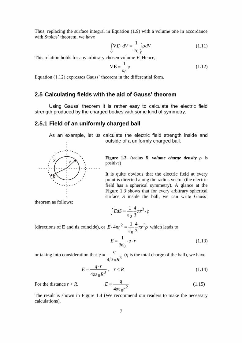
2.5.1 Field of an uniformly charged ball

As an example, let us calculate the electric field strength inside and outside of a uniformly charged ball.

Figure 1.3. (radius R, volume charge density is

positive)

It is quite obvious that the electric field at every

point is directed along the radius vector (the electric

field has a spherical symmetry). A glance at the

Figure 1.3 shows that for every arbitrary spherical

surface S inside the ball, we can write Gauss’

theorem as follows:

3

0 3

41rEdS

(directions of E and ds coincide), or

3

0

2

3

414 rrE which leads to

rE

03

1 (1.13)

or taking into consideration that 334 R

q

(q is the total charge of the ball), we have

304 R

rqE

, r < R (1.14)

For the distance r > R, 2

04 r

qE

(1.15)

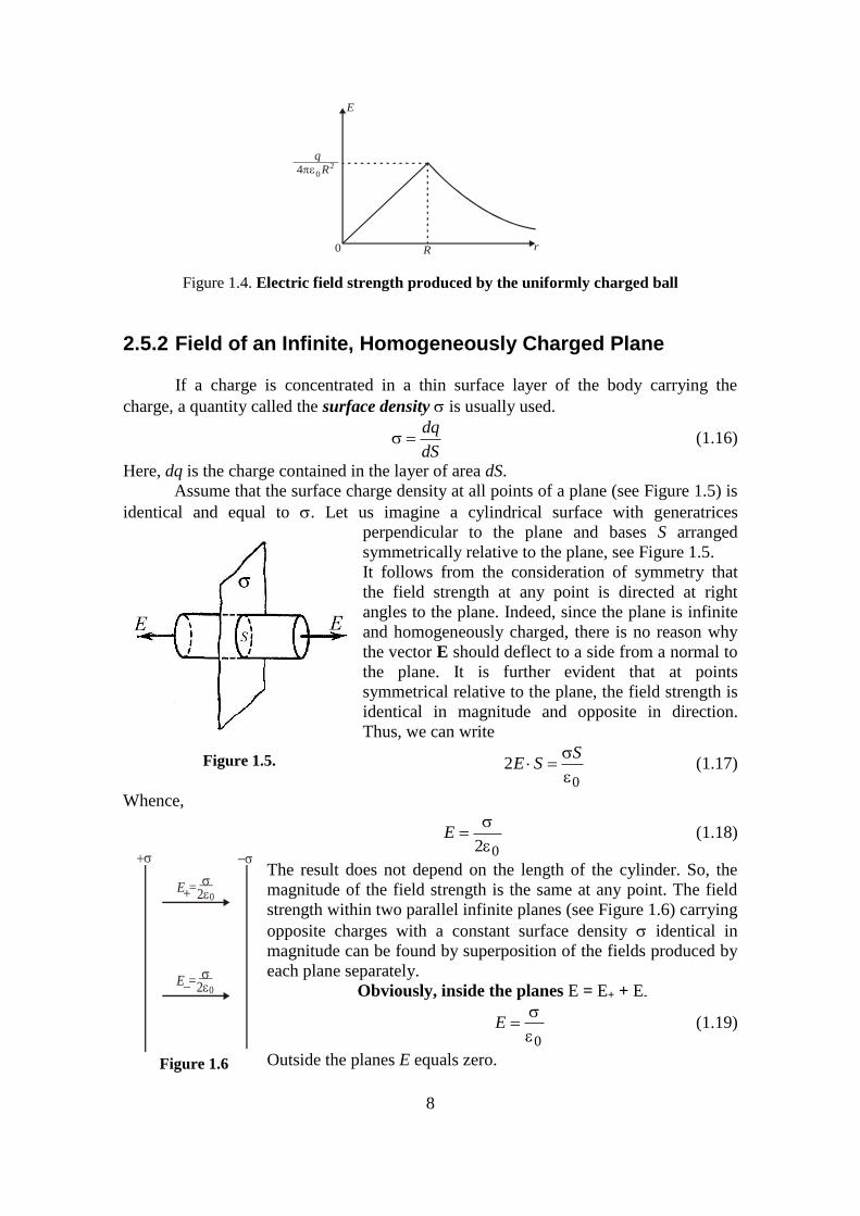
The result is shown in Figure 1.4 (We recommend our readers to make the necessary

calculations).

R

rS

8

Figure 1.4. Electric field strength produced by the uniformly charged ball

2.5.2 Field of an Infinite, Homogeneously Charged Plane

If a charge is concentrated in a thin surface layer of the body carrying the

charge, a quantity called the surface density is usually used.

dS

dq (1.16)

Here, dq is the charge contained in the layer of area dS.

Assume that the surface charge density at all points of a plane (see Figure 1.5) is

identical and equal to . Let us imagine a cylindrical surface with generatrices

perpendicular to the plane and bases S arranged

symmetrically relative to the plane, see Figure 1.5.

It follows from the consideration of symmetry that

the field strength at any point is directed at right

angles to the plane. Indeed, since the plane is infinite

and homogeneously charged, there is no reason why

the vector E should deflect to a side from a normal to

the plane. It is further evident that at points

symmetrical relative to the plane, the field strength is

identical in magnitude and opposite in direction.

Thus, we can write

0

2

SSE (1.17)

Whence,

02

E (1.18)

The result does not depend on the length of the cylinder. So, the

magnitude of the field strength is the same at any point. The field

strength within two parallel infinite planes (see Figure 1.6) carrying

opposite charges with a constant surface density identical in

magnitude can be found by superposition of the fields produced by

each plane separately.

Obviously, inside the planes E = E+ + E-

0

E (1.19)

Outside the planes E equals zero.

q

4R02

E

rR0

E = +

__20

E = __

20

Figure 1.5.

Figure 1.6

9

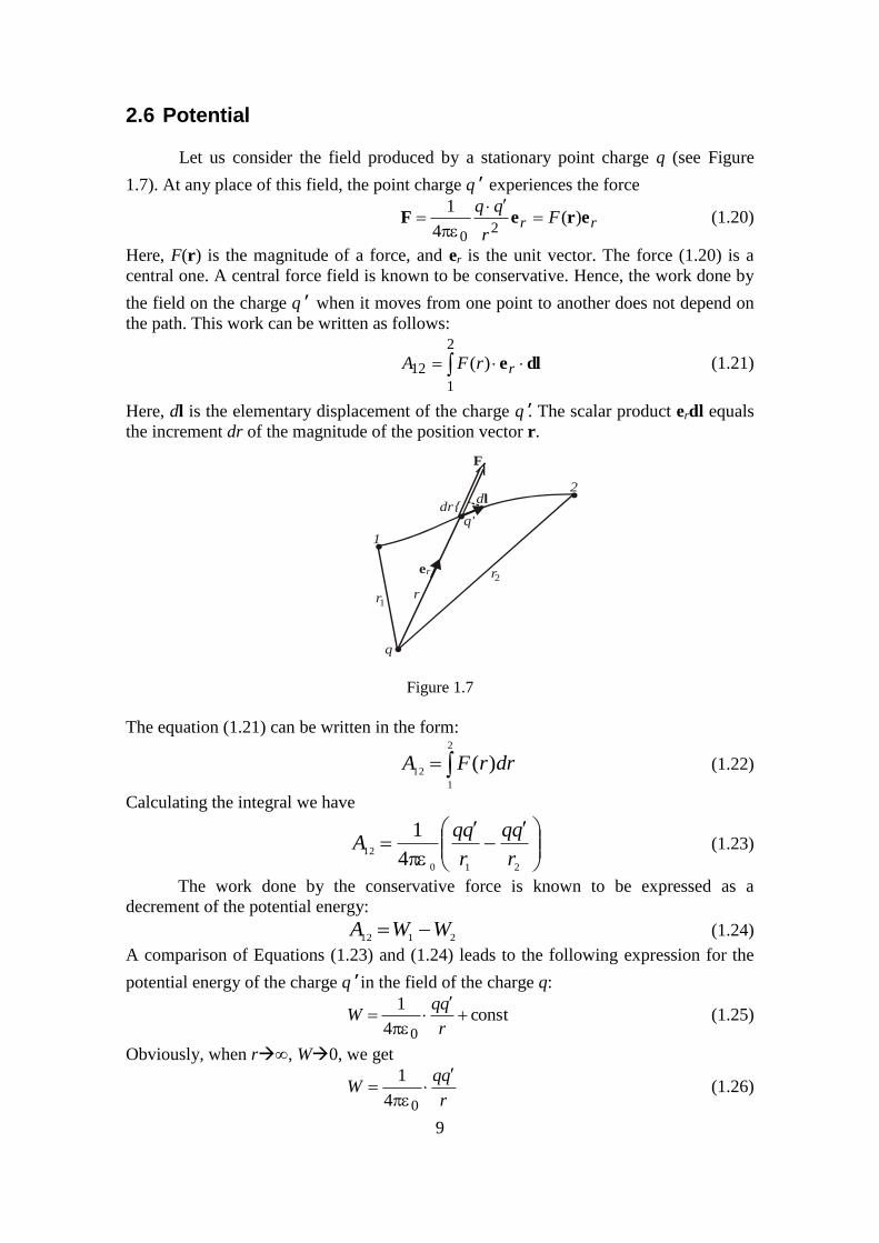
2.6 Potential

Let us consider the field produced by a stationary point charge q (see Figure

1.7). At any place of this field, the point charge q' experiences the force

rr Fr

qqereF )(

4

1

20

(1.20)

Here, F(r) is the magnitude of a force, and er is the unit vector. The force (1.20) is a

central one. A central force field is known to be conservative. Hence, the work done by

the field on the charge q' when it moves from one point to another does not depend on

the path. This work can be written as follows:

2

1

12 )( dlerrFA (1.21)

Here, dl is the elementary displacement of the charge q'. The scalar product erdl equals

the increment dr of the magnitude of the position vector r.

Figure 1.7

The equation (1.21) can be written in the form:

2

1

12)( drrFA (1.22)

Calculating the integral we have

210

124

1

r

qq

r

qqA (1.23)

The work done by the conservative force is known to be expressed as a

decrement of the potential energy:

2112WWA (1.24)

A comparison of Equations (1.23) and (1.24) leads to the following expression for the

potential energy of the charge q' in the field of the charge q:

const4

1

0

r

qqW (1.25)

Obviously, when r, W0, we get

r

qqW

04

1 (1.26)

..

.

.{1

2

q

r r

r

1

2er

drdl

q'

F

10

The quantity = W/q' is called the field potential at a given point, and it is used

together with the field strength E to describe electric field. So, the potential produced by

a point charge q at a distance r is

r

q

04

1 (1.27)

Using the superposition principle we get:

N

i i

i

r

q

104

1 (1.28)

The equation (1.28) signifies that the potential of the field produced by a system of

charges equals the algebraic sum of the potentials produced by each of the charges

separately. Whereas, the field strengths are added vectorially in the superposition of

fields, the potentials are added algebraically. This is why it is usually more convenient

to calculate the potentials than the electric field strengths. The work of the field forces

on the charge q can be expressed as follows:

)(2112

qA (1.29)

If the charge q is removed from a point having the potential to infinity, then

qA (1.30)

Hence, the potential numerically equals the work done by the forces of a field on a unit

positive point charge when the latter is removed from the given point to infinity. Work

of the same magnitude must be done against the electric field forces to move a unit

positive point of a field. Equation (1.30) can be used to establish the units of potential.

The SI unit of potential called the volt (V) is taken equal to the potential at a point when

work of 1 joule has to be done to move a charge of 1 coulomb from infinity to this point

1J = 1C1V. Whence,

1C

1JV1 (1.31)

2.7 Relations between the electric field strength and potential

This relation can be easily established using the relevant relation between the

force and potential energy of conservative fields.

WW gradF (1.32)

For a charged particle in an electrostatic field, we have F=qE and W=q. Introducing

these values into equation (1.32), we find that

gradE (1.33)

when an electric charge moves along the closed path, the work done is zero

0lE dqA (1.34)

The quantity

lEd is called the circulation of an electrostatic field.

0

lEd (1.35)

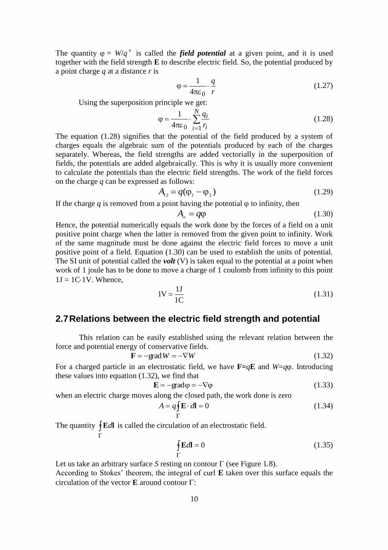
Let us take an arbitrary surface S resting on contour (see Figure 1.8).

According to Stokes’ theorem, the integral of curl E taken over this surface equals the

circulation of the vector E around contour :

11

Figure 1.9

lEddSE

S

][ (1.37)

Since the circulation equals zero, then

0][

S

dSE (1.38)

This condition holds for any surface S rested on

arbitrary contour . This is possible only if the curl of

the vector E at every point of the electrostatic field

equals zero:

0][ E (1.39 )

2.8 Equipotential Surfaces and Strength Lines

Graphically an electrostatic field can be characterized by the equipotential

surfaces and strength lines. An imaginary surface all of whose points have the same

potential is called the equipotential surface. Its equation has the form:

(x, y, z) = const (1.40)

The strength lines are imaginary lines drawn in such a way that a tangent to them at

every point coincides with the direction of vector E. The density of the lines is selected

so that their number passing through a unit area at right angles to the lines, equals the

numerical value of vector E. Thus, the potential does not change in movement along an

equipotential surface over the distance dl (d). Hence, the tangential component of

vector E equals zero:

0

lE

l (1.41)

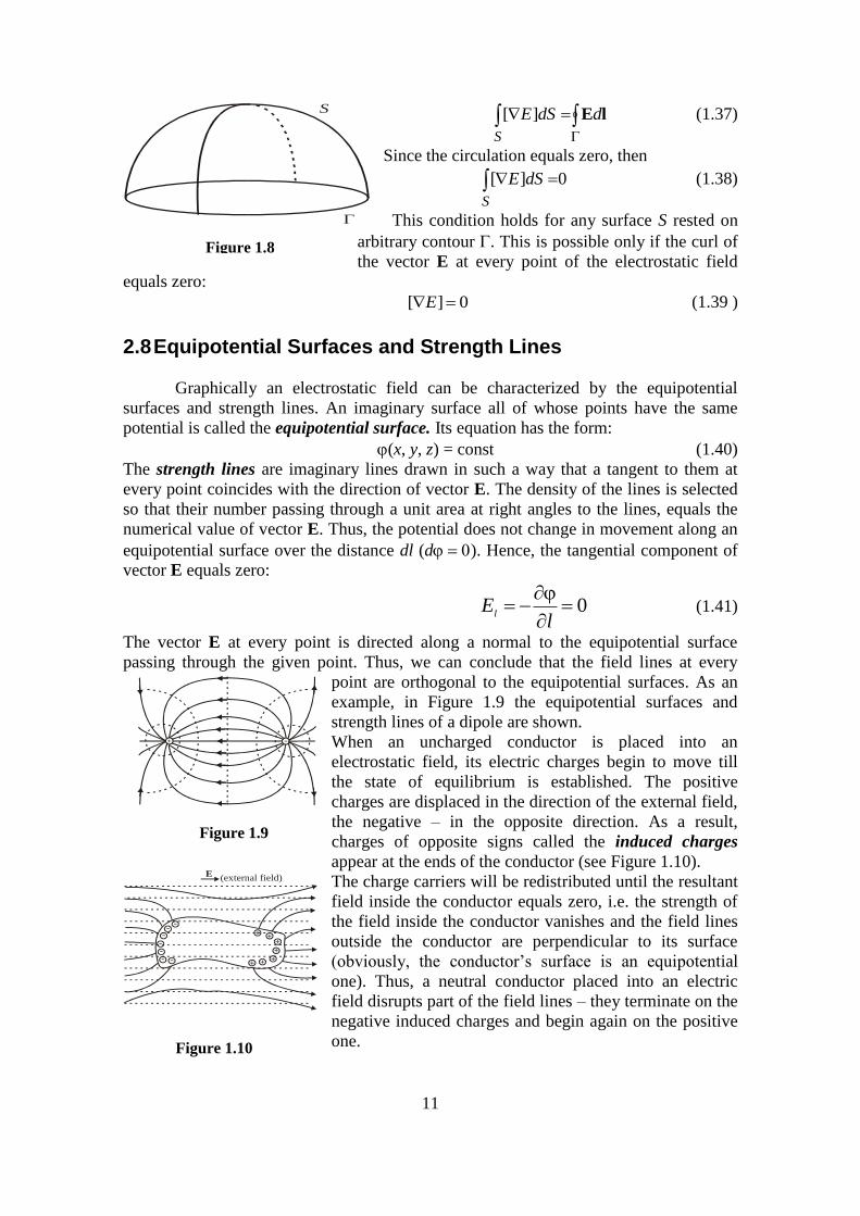
The vector E at every point is directed along a normal to the equipotential surface

passing through the given point. Thus, we can conclude that the field lines at every

point are orthogonal to the equipotential surfaces. As an

example, in Figure 1.9 the equipotential surfaces and

strength lines of a dipole are shown.

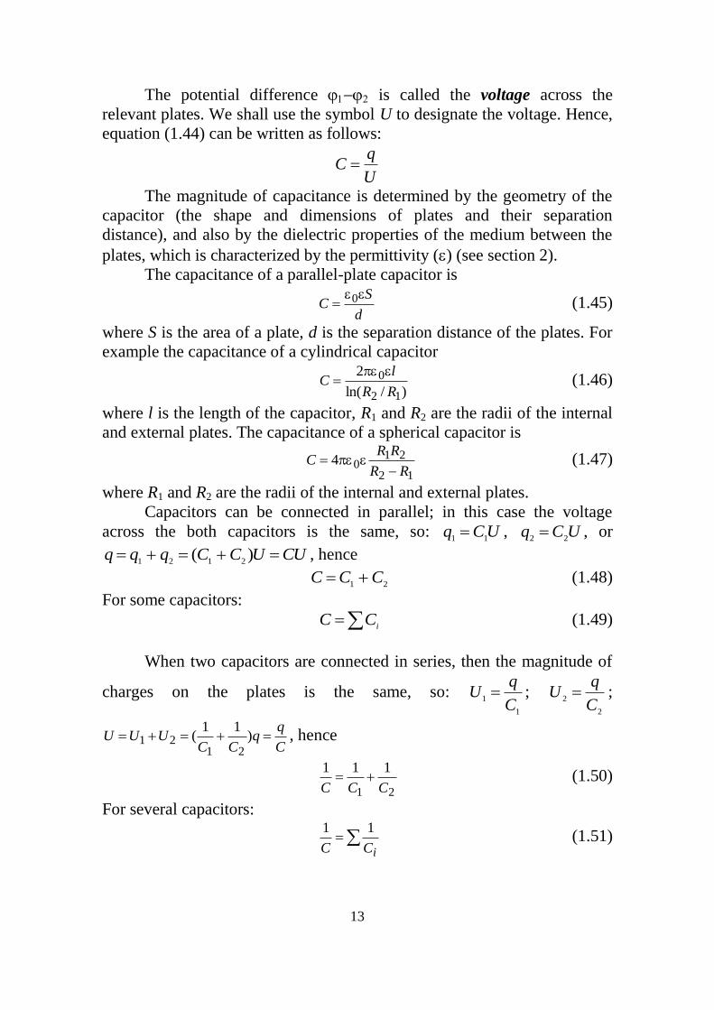
When an uncharged conductor is placed into an

electrostatic field, its electric charges begin to move till

the state of equilibrium is established. The positive

charges are displaced in the direction of the external field,

the negative – in the opposite direction. As a result,

charges of opposite signs called the induced charges

appear at the ends of the conductor (see Figure 1.10).

The charge carriers will be redistributed until the resultant

field inside the conductor equals zero, i.e. the strength of

the field inside the conductor vanishes and the field lines

outside the conductor are perpendicular to its surface

(obviously, the conductor’s surface is an equipotential

one). Thus, a neutral conductor placed into an electric

field disrupts part of the field lines – they terminate on the

negative induced charges and begin again on the positive

one.

S

+- + ++

+++

-----

-

E (external field)

Figure 1.10

+ -

Figure 1.8

12

1.9. Capacitance

If a conductor is isolated, i.e. the other bodies are very far from it,

then the experiments show that the charge and potential of the conductor

are proportional one another.

Cq (1.42)

A quantity

qC (1.43)

is called the capacitance. In accordance with Equation (1.43), it follows

that the capacitance numerically equals the charge which when imparted to

a conductor increases its potential by unity (1V). SI-unit of capacitance is a

farad (F). The farad is a very big unit. Indeed, an isolated sphere having a

radius of 9109 m, i.e. a radius 1500 times greater than that of the Earth,

would have the capacitance of 1 F. For this reason, submultiples of farad

are used in practice – the millifarad (mF), microfarad (F), nanofarad (nF),

and picofarad (pF).

Isolated conductors have a small capacitance. However, such devices

are needed in practice which with a low potential relative to the

surrounding bodies would accumulate charges of an appreciable

magnitude. Such devices, called capacitors, are based on the fact that the

capacitance of a conductor increases when other bodies are brought close to

it. This in its turn is due to the fact that induced charges of the sign opposite

to that of the conductor will be closer to the conductor than charges of the

same sign, thus diminishing the conductor’s potential and in accordance

with equation (1.43) increasing its capacitance. Capacitors are made in the

form of two conductors placed close to each other. The conductors forming

a capacitor are called its plates, which can be made in the form of two

plates, two coaxial cylinders, and two concentric spheres. Accordingly,

they are called parallel-plate, cylindrical, and spherical capacitors. The

electrostatic field is confined inside a capacitor. The strength (in general

case, the electric displacement (see section 2)) lines begin on one plate and

finish on the other. Consequently, the charges produced on the plates have

the same magnitude and are opposite in sign.

The basic characteristic of a capacitor is its capacitance, by which is

meant a quantity proportional to the charge q and inversely proportional to

the potential difference between the plates:

21

qC (1.44)

13

The potential difference is called the voltage across the

relevant plates. We shall use the symbol U to designate the voltage. Hence,

equation (1.44) can be written as follows:

U

qC

The magnitude of capacitance is determined by the geometry of the

capacitor (the shape and dimensions of plates and their separation

distance), and also by the dielectric properties of the medium between the

plates, which is characterized by the permittivity () (see section 2).

The capacitance of a parallel-plate capacitor is

d

SC

0 (1.45)

where S is the area of a plate, d is the separation distance of the plates. For

example the capacitance of a cylindrical capacitor

)/ln(

2

12

0

RR

lC

(1.46)

where l is the length of the capacitor, R1 and R2 are the radii of the internal

and external plates. The capacitance of a spherical capacitor is

12

2104

RR

RRC

(1.47)

where R1 and R2 are the radii of the internal and external plates.

Capacitors can be connected in parallel; in this case the voltage

across the both capacitors is the same, so: UCq11

, UCq22

, or

CUUCCqqq )(2121

, hence

21CCC (1.48)

For some capacitors:

iCC (1.49)

When two capacitors are connected in series, then the magnitude of

charges on the plates is the same, so: 1

1C

qU ;

2

2C

qU ;

C

qq

CCUUU )

11(

2121 , hence

21

111

CCC (1.50)

For several capacitors:

iCC

11 (1.51)

14

1.10 Interaction Energy of a System of Charges

In accordance with equation (1.19), the interaction energy of a

system of charged particles can be written in the form:

)( 04

1

2

1

ki ik

ki

r

qqW , (1.52)

where rik is the distance between the qi and qk charges. The factor “1/2” is

necessary in order not to take into account the Wik two times. Equation

(1.52) can be rewritten as follows:

)( 1 04

1

2

1

i k ik

ki

r

qqW (1.53)

The expression

104

1

k ik

ki

r

q (1.54)

describes the potential produced by all the charges except qi at the point

where the charge qi is located. Thus, we get the interaction energy in the

form:

N

iiiqW

12

1 (1.55)

1.11 Energy of a Charged Conductor

The charge q on a conductor can be considered as a system of point

charges qi. The surface of a conductor is equipotential. Thus, having in

mind the expression (1.46) we can write

222

1 22

C

C

qqW (1.56)

1.12 Energy of a Charged Capacitor

Assume the potential of a capacitor plate carrying the charge +q is

1, and that of a plate carrying the charge –q is 2. Then, using the

expression (1.55) we get

22

2

1)(

2

1)()(

2

1

22

2121

CU

C

q

qUqqqW

(1.57)

Having in mind that U/d=E, Sd=V and the capacitance of a parallel-plate

capacitor d

SC

0 , we can rewrite the equation (1.57) in the form

15

VVE

W

2

20 , (1.58)

where, the energy density

2

20 E

(1.59)

Equation (1.59) holds everywhere.

Examples

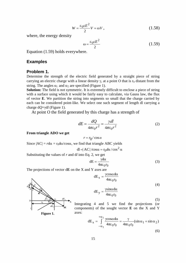
Problem 1. Determine the strength of the electric field generated by a straight piece of string

carrying an electric charge with a linear density , at a point O that is r0 distant from the

string. The angles and are specified (Figure 1).

Solution: The field is not symmetric. It is extremely difficult to enclose a piece of string

with a surface using which it would be fairly easy to calculate, via Gauss law, the flux

of vector E. We partition the string into segments so small that the charge carried by

each can be considered point-like. We select one such segment of length dl carrying a

charge dQ=dl (Figure 1).

At point O the field generated by this charge has a strength of

20

20 44 rπε

γdl

rπε

dQdE (2)

From triangle ADO we get

α/rr cos0

Since |AC| = rd= r0d/cos, we find that triangle ABC yields

20 cos//cos|AC|dl dr

Substituting the values of r and dl into Eq. 2, we get

004π

ddE

r

(3)

The projections of vector dE on the X and Y axes are

00x

4π

dcosdE

r

(4)

00y

4π

dsindE

r

(5)

Integrating 4 and 5 we find the projections (or

components) of the sought vector E on the X and Y

axes:

)sin(sin4π4π

dcosdE 21

0000x

1

1

rr

(6)

.

.

.

.

.

X

Y

dE

dE

dE

x

y

Dr

0 1

d

2

A

BC

dl

r

O

Figure 1.

16

)cos(cos4π4π

dsindE 21

0000y

1

1

rr

(7)

Clearly, the field generated by a charged infinitely straight string, constitutes a

particular case of the field generated by a piece of charged straight string. Indeed, for

and Eq. 6 and 7 yield Ex=r0 and Ey=0.

Problem 2. An infinitely long string uniformly charged with a linear density 1=+310

-7 C/m and a

segment of length l = 20 cm uniformly charged with a linear density 2=+210-7

C/m lie

in a plane at right angles to each other and separated by a distance r0=10 cm. Determine

the force with which these two bodies interact.

Solution: Two objects constitute the physical system, the infinitely long string and the

segment. Neither of the two can be considered a particle. The physical phenomenon

consists of the effect that the field of the string has on the charge of the segment. We

wish to find the force of this interaction. The charge Q2 = 2l carried by the segment is

positioned in the electric field of the string, which is known.

It would seem that to find the force acting on the charge we need only use the formula

F = Q2E, where E = 1/2r0. This is not correct, however, since the formula is valid

also in the case of a point charge (Q2 is distributed over the segment). On different

sections (of equal length) of the segment of length l different forces are acting.

Therefore, to calculate the force with which the nonhomogeneous field generated by the

string acts on the distributed charge Q2 we use the method of differentiation and

successive integration. We partition segment l into sections of length dx so small that

the charge dQ=2dx of each section can be considered a point charge. The charge dQ is

in the electric field of the string. Since this is a point charge, the force acting on it is

xx

QEF d2π

dd0

21

where x is the distance from charge dQ to the string.

We now have the differential of the sought quantity. The force acting on each section of

the segment depends on the distance x from the segment to the string, and so we select x

as the variable of integration (it varies from x1 = r0 to x2 = r0 + l). Integrating previous

equation with respect to x, we get

lr

rr

xx

0

0

)l

1ln(2π

d2π

F00

21

0

21

Substitution of numerical values yields the result F 1.210-3

N.

The terms of the above problem can be changed by placing the segment parallel to the

string, at an angle to the string, in a plane perpendicular to the string, and so on. All

these variants can be solved by the same method.

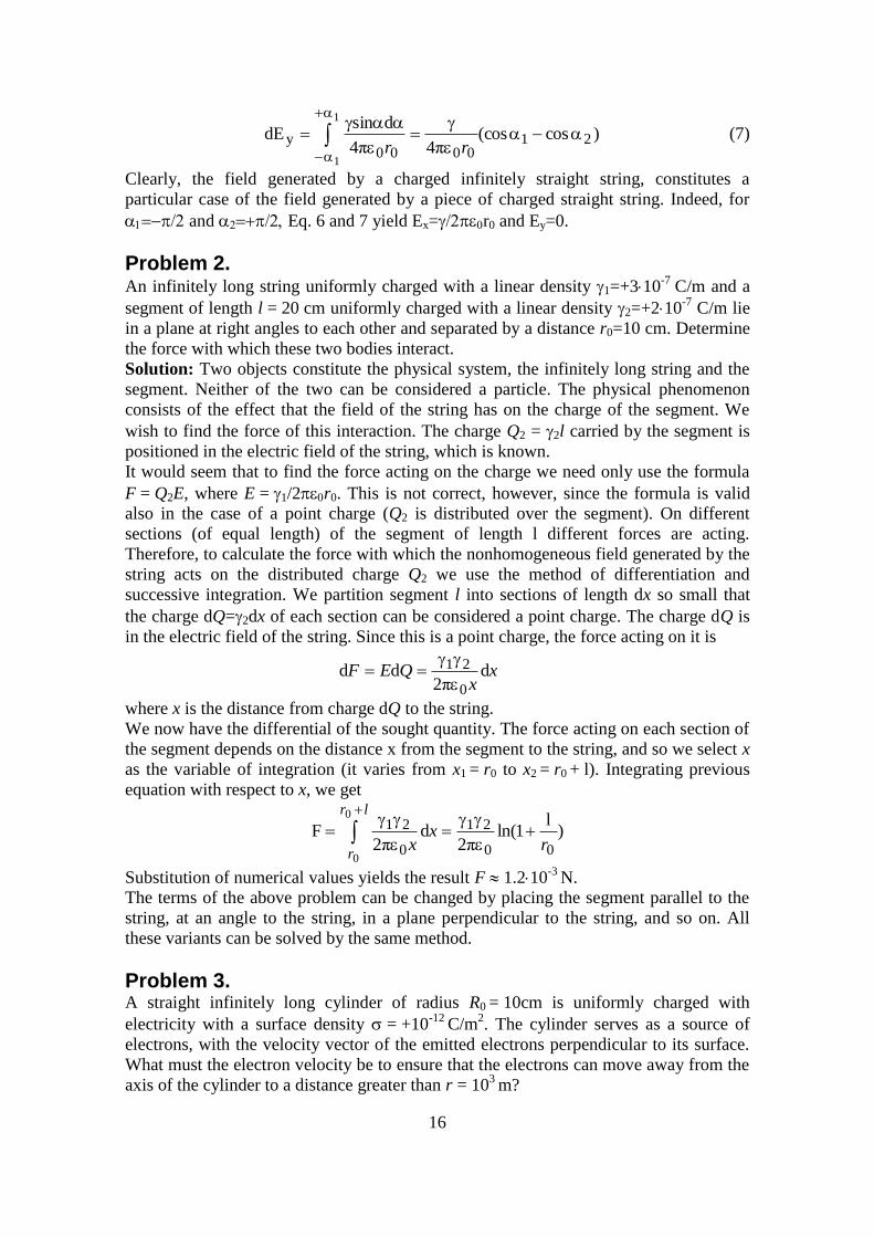
Problem 3. A straight infinitely long cylinder of radius R0 = 10cm is uniformly charged with

electricity with a surface density = +10-12

C/m2. The cylinder serves as a source of

electrons, with the velocity vector of the emitted electrons perpendicular to its surface.

What must the electron velocity be to ensure that the electrons can move away from the

axis of the cylinder to a distance greater than r = 103

m?

17

Solution: The physical system consists of two objects: the positively charged cylinder

and an electron. The physical phenomenon consists of the electron moving in a

decelerated manner in the electric field of the cylinder. We wish to find one of the

parameters of motion, the electron velocity.

To describe the motion of the electron we must first calculate the electric field of the

cylinder. The charge on the cylinder cannot be considered a point charge. We apply

Gauss’ law. For this we surround the cylinder with a cylindrical surface (coaxial with

the cylinder) of an arbitrary radius r > R0 (Figure 3). In view of the symmetry of the

problem, the electric vector E of the field of the cylinder is perpendicular at all points to

the constructed cylindrical surface. Hence, the flux of E out of the cylindrical surface of

length l is

rlEE 2

By Gauss’ theorem,

00 σ/22 lRrlE

whence

r

RE

0

0σ

(1)

Now, by applying the dynamical method we find that

Newton’s second law yields

r

Re

t

rm

0

0

2

2

ed

d

,

where me is the electron mass, and e is the electron

charge. From the standpoint of physics the problem is

solved.

It would be solved completely if we were to solve the above differential equation and

obtain the law of motion of the electron r = r(t). Knowing this law, we could find the

law of variation of the electron’s velocity with time, v = r(t), and so on. But instead let

us apply the law of energy conservation. By this law,

eevm

0

20e

2, (2)

where 0 is the potential of the cylinder, and the potential of the field of the cylinder

at a point r distant from the cylinder’s axis. Employing the relationship E = -ddr that

exists between the field strength E and potential and allowing for Eq.1, we arrive at

the following differential equation:

rr

R

d

dσ

0

0

.

Integrating, we find that

СrR

lnσ

0

0 (3)

with C being an arbitrary constant. Hence,

СRR

00

00 ln

σ (4)

The system of Equations 2,3,4 yields the following value for the sought initial velocity

of electron:

R0

r

l

Figure 3

18

ra

a

r

a

b

E

ra

E=r

k Qe

2

__

m/s. 103.7 ,ε

)ln(σ2 50

e0

000 v

m

r/ReRv

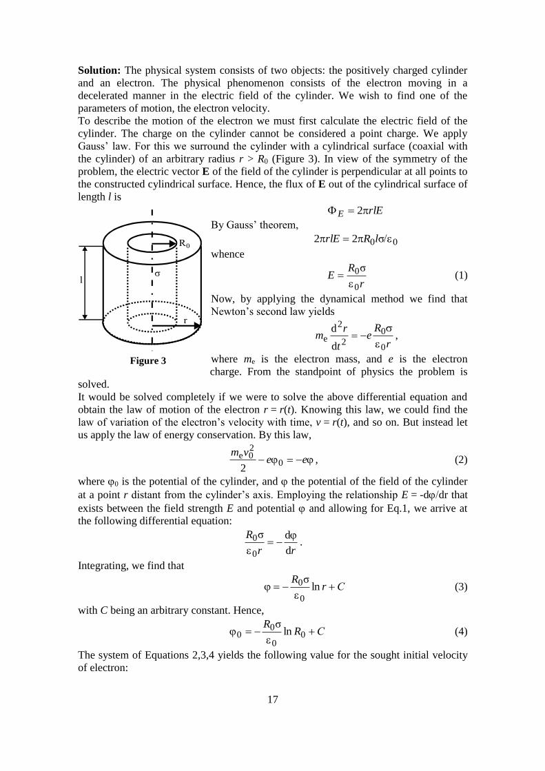
Problem 4 An insulating sphere of radius a has a uniform

charge density and a total positive charge Q (see

Figure 4). (a) Calculate the magnitude of the electric

field at a point outside the sphere.

Solution: Since the charge distribution is spherically

symmetric, we select a spherical gaussian surface of

radius r, concentric with the sphere, as in Fig.4a.

Gauss’ law gives

0

qEdAdc AE

By symmetry, E is constant everywhere on the surface, and so it can be removed from

the integral Therefore

00

32 1ρπ

3

4)π4(

QarEdAEEdA

where we have used the fact that the surface area of a sphere is 4r2. Hence, the

magnitude of the field at a distance r from the center of the sphere

2204 r

Qk

r

QE e

(for r>a)

Note that this result is identical to that obtained for a point charge. Therefore, we

conclude that, for a uniformly charged sphere, the field in the region external to the

sphere is equivalent to that of a point charge located at the center of the sphere.

(b) Find the magnitude of the electric field at a point inside the sphere.

Reasoning and Solution: In this case we select a spherical gaussian surface with radius

r<a, concentric with the charge distribution (see Figure 4b). Let us denote the volume

of this smaller sphere by V'. To apply Gauss’ law in this situation, it is important to

recognize that the charge qin within the gaussian surface of volume V' is a quantity less

than the total charge Q. To calculate the charge qin, we use the fact that qin=V', where

is the charge per unit volume and V' is the volume enclosed by the gaussian surface,

given by V' = 4/3r3 for a sphere. Therefore,

)34( 3rVqin

On Figure 4: A uniformly charged insulating sphere of radius a and total charge

Q. (a) The field at a point exterior to the sphere is keQ/r2. (b) The

field inside the sphere is due only to the charge within the gaussian

surface and is given by (keQ/a3)r.

A plot of E versus r for a uniformly charged insulating sphere. The

field inside the sphere (r<a) varies linearly with r. The field

outside the sphere (r>a) is the same as that of a point charge Q

located at the origin.

Figure 4

19

The magnitude of the electric field is constant everywhere on the spherical gaussian

surface and is normal to the surface at each point. Therefore, Gauss’ law in the region

r<a gives

0

2 )4(

inqrEdAEEdA

Solving for E gives

rr

r

r

qE in

02

0

3

20

34

3

4

4

Since by definition 3

3

4/ aQ , this can be written

ra

Qk

a

QrE

3

3

304

(for r<a)

Note that this result for E differs from that obtained in part (a). It shows that E0 as

r0, as you might have guessed based on the spherical symmetry of the charge

distribution. Therefore, the result fortunately eliminates the singularity that would exist

at r = 0 if E varied as 1/r2 inside the sphere. That is, if E1/r

2, the field would be

infinite at r = 0, which is clearly a physically impossible situation. A plot of E versus r

is shown in Figure 4.

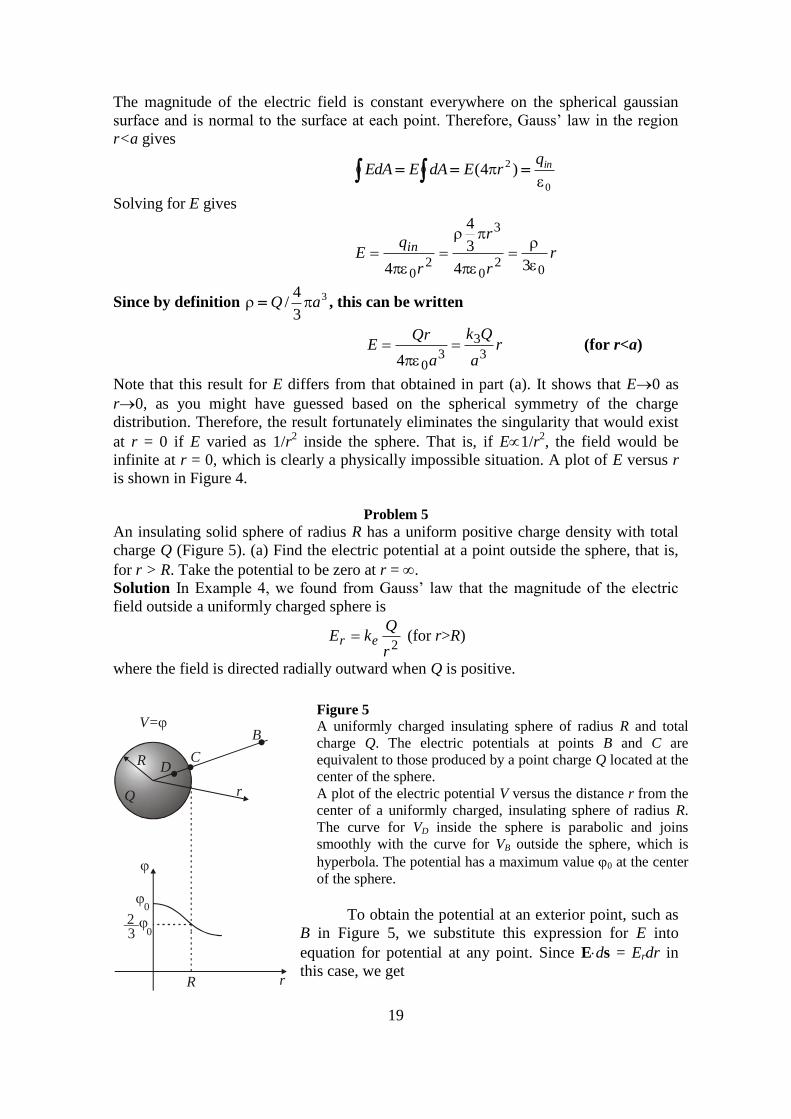
Problem 5

An insulating solid sphere of radius R has a uniform positive charge density with total

charge Q (Figure 5). (a) Find the electric potential at a point outside the sphere, that is,

for r > R. Take the potential to be zero at r = .

Solution In Example 4, we found from Gauss’ law that the magnitude of the electric

field outside a uniformly charged sphere is

2r

QkE er (for r>R)

where the field is directed radially outward when Q is positive.

To obtain the potential at an exterior point, such as

B in Figure 5, we substitute this expression for E into

equation for potential at any point. Since Eds = Erdr in

this case, we get

Figure 5

A uniformly charged insulating sphere of radius R and total

charge Q. The electric potentials at points B and C are

equivalent to those produced by a point charge Q located at the

center of the sphere.

A plot of the electric potential V versus the distance r from the

center of a uniformly charged, insulating sphere of radius R.

The curve for VD inside the sphere is parabolic and joins

smoothly with the curve for VB outside the sphere, which is

hyperbola. The potential has a maximum value 0 at the center

of the sphere.

R ..

.B

CD

rQ

V=

R r

0

023

__

20

r

er

r

r

Br

drQkdrEdV

2sE

r

QkV eB (for r>R)

Note that the result is identical to that for the electric potential due to a point charge.

Since the potential must be continuous at r = R, we can use this expression to obtain the

potential at the surface of the sphere. That is, the potential at a point such as C in Fig.5

is

R

QkV eC (for r=R)

(b) Find the potential at a point inside the charged sphere, that is, for r<R.

Solution In Example 12 we found that the electric field inside a uniformly charged

sphere is

rR

QkE er 3

(for r<R)

We can use this result to evaluate the potential difference VD VC, where D is an

interior point:

r

Reer

R rCD rRR

Qkrdr

R

QkdrEVV )(

2

22

33

Substituting VC = keQ/R into this expression and solving for VD, we get

)3(2 2

2

R

r

R

QkV e

D (for r<R)

At r = R, this expression gives a result for the potential that agrees with that for the

potential at the surface, that is, VC. A plot of V versus r for this charge distribution is

given in Figure 5.

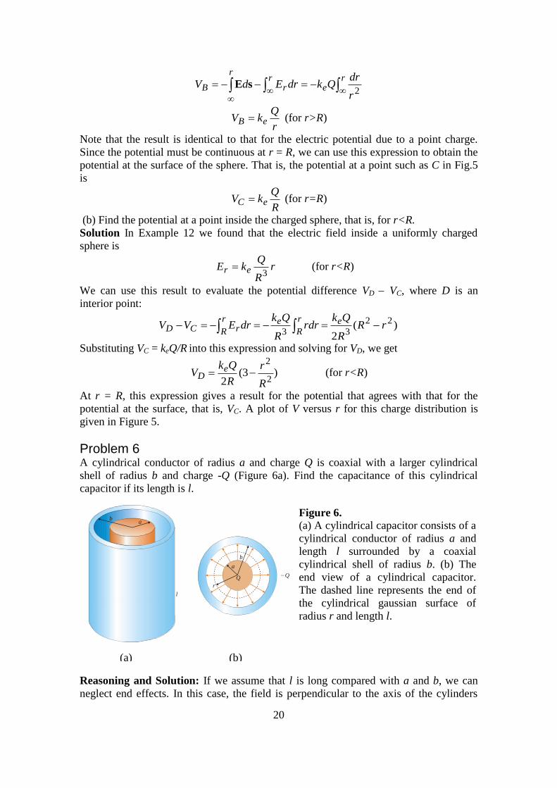
Problem 6 A cylindrical conductor of radius a and charge Q is coaxial with a larger cylindrical

shell of radius b and charge -Q (Figure 6a). Find the capacitance of this cylindrical

capacitor if its length is l.

Reasoning and Solution: If we assume that l is long compared with a and b, we can

neglect end effects. In this case, the field is perpendicular to the axis of the cylinders

Figure 6.

(a) A cylindrical capacitor consists of a

cylindrical conductor of radius a and

length l surrounded by a coaxial

cylindrical shell of radius b. (b) The

end view of a cylindrical capacitor.

The dashed line represents the end of

the cylindrical gaussian surface of

radius r and length l.

ba

l

Q_a

b

r

Q

(a) (b)

(a) (b)

21

and is confined to the region between them (Figure 6 b). We must first calculate the

potential difference between the two cylinders, which is given in general by

b

aab dVV sE

where E is the electric field in the region a<r<b. The electric field of a cylinder of

charge per unit length is E = 2ker. The same result applies here, since the outer

cylinder does not contribute to the electric field inside it. Using this result and noting

that E is along r in Figure 6b, we find that

)ln(22a

bk

r

drkdrEVV e

b

a

b

aerab

Substituting this into equation for the capacitance and using the fact that = Q/l, we get

)ln(2)ln(2

a

be

a

be k

l

l

Qk

Q

V

QC

where V is the magnitude of the potential difference, given by 2keln(b/a), a positive

quantity. That is, V = Va – Vb is positive because the inner cylinder is at the higher

potential. Our result for C makes sense because it shows that the capacitance is

proportional to the length of the cylinder. As you might expect, the capacitance also

depends on the radii of the two cylindrical conductors. As an example, a coaxial cable

consists of two concentric cylindrical conductors of radii a and b separated by an

insulator. The cable carries currents in opposite directions in the inner and outer

conductors. Such a geometry is especially useful for shielding an electrical signal from

external influences. From the latter equation we see that the capacitance per unit length

of a coaxial cable is

)ln(2

1

a

bekl

C .

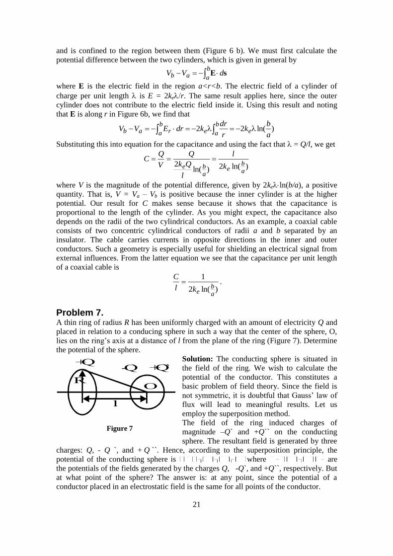
Problem 7. A thin ring of radius R has been uniformly charged with an amount of electricity Q and

placed in relation to a conducing sphere in such a way that the center of the sphere, O,

lies on the ring’s axis at a distance of l from the plane of the ring (Figure 7). Determine

the potential of the sphere.

Solution: The conducting sphere is situated in

the field of the ring. We wish to calculate the

potential of the conductor. This constitutes a

basic problem of field theory. Since the field is

not symmetric, it is doubtful that Gauss’ law of

flux will lead to meaningful results. Let us

employ the superposition method.

The field of the ring induced charges of

magnitude –Q` and +Q`` on the conducting

sphere. The resultant field is generated by three

charges: Q, - Q `, and + Q ``. Hence, according to the superposition principle, the

potential of the conducting sphere is where are

the potentials of the fields generated by the charges Q, -Q`, and +Q``, respectively. But

at what point of the sphere? The answer is: at any point, since the potential of a

conductor placed in an electrostatic field is the same for all points of the conductor.

Figure 7

+Q+Q̀̀-Q̀

l

OR

22

In our case, the entire volume bound by the conducting sphere as equipotential. Thus,

we need only calculate the potential at the most convenient point, the center of the

sphere. Indeed, notwithstanding the fact that we know neither the values of the induced

charges –Q` and +Q`` nor the distributions of the respective charge densities -` and

+`` over the sphere, we can state that the total potential of the field of these charges at

the special point (the center of the sphere) is zero: (the induced charges

–Q` and +Q`` lie at equal distances from the center of the sphere, are equal in

magnitude, |-Q`| = |+Q``|, and are opposite in sign). Hence, we need only to calculate

the potential 1 of the ring’s field at O (Figure 7):

1/2220

1)(l4π R

Q

.

This constitutes the potential of the sphere, .

23

Electric Field in Dielectrics 2.1. Dipole Electric Moment

In a strict sense, dielectrics (or insulators) are substances which cannot conduct

an electric current. Ideal isolators do not exist in nature. All substances, even of to a

negligible extent, conduct an electric current. But substances called conductors conduct

a current from 1015

to 1020

times better than substances called dielectrics.

A molecule is a system with a total charge of zero. To characterize its electrical

properties, the quantity called the dipole electric moment (p) is used:

iiq rp (2.1)

(summation is performed both over the electrons and nuclei). If the system has the total

electric charge equal to zero, the magnitude of the dipole moment does not depend on

the choice of the coordinate system origin. Indeed, let us make a transformation

ar ii

r , (2.2)

where a is the shift of the coordinate origin. Obviously,

pararrp iiiiiiiqqqq )( (2.3)

The electrons in a molecule are in motion, and the quantity (2.3) constantly

changes. The velocities of electrons are so high, however, that the mean value of the

dipole moment(2.3) is detected in practice:

ii

q rp . (2.4)

In other words, we shall consider that the electrons are at rest relative to the nuclei at

certain points obtained by averaging the positions of the electrons in time.

The behavior of a molecule in an external electric field is determined by its

dipole moment. Let us calculate the potential energy of a molecule located in an

external field. Having in mind that the magnitude of <ri> is small, we can write the

potential at the point where i-th charge is in the form

ii

r . (2.5)

Hence,

iiiiiii

qqqqW rr )( (2.6)

Taking into account that 0i

q and substituting –E for we arrive at

cospEW pE . (2.7)

Differentiating this expression with respect to we get the rotational momentum

(torque) T=pEsin, or in the vector form:

pET . (2.8)

Differentiating Equation (2.7) with respect to linear coordinates (x, y, z) we get

the force acting on the dipole. For example, when a dipole is located in an

inhomogeneous field that is symmetric relative to the x-axis,

0 ;cos

zyxFF

x

Ep

x

WF . (2.9)

Here, is an angle between p and E. For a system containing only two charges +q and

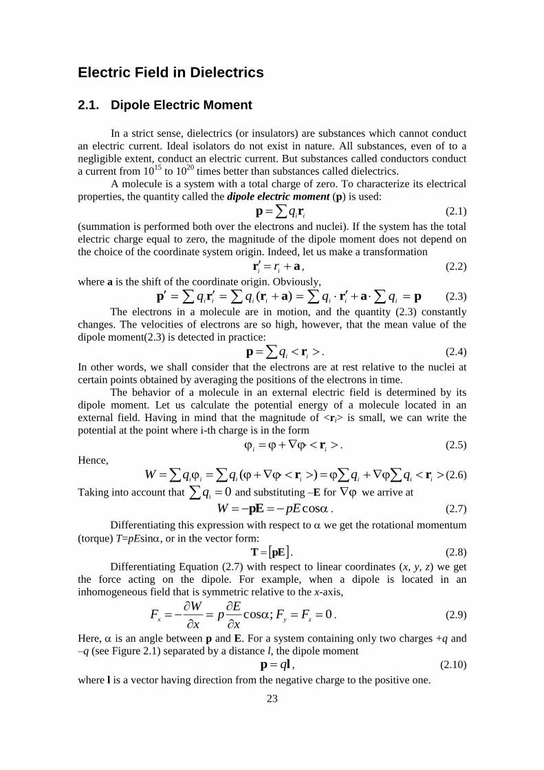
–q (see Figure 2.1) separated by a distance l, the dipole moment

lp q , (2.10)

where l is a vector having direction from the negative charge to the positive one.

24

Figure 2.1.

2.2 Polar and Non-polar Molecules

The interpretation of any real system by two charges of different signs holds if

we mean by –q and +q the centers (rc) of the spherical distribution, correspondingly, of

the negative and positive charges:

dV

q

c

iic

rr

rr or ,} (2.11)

(summation or integration is taken over only the charges of the same sign).

In symmetrical molecules (such as H2, O2, N2), the centers of the spatial

distribution of the positive and negative charges coincide in the absence of an external

electric field. These molecules have no intrinsic dipole moments and are called non-

polar. In asymmetrical molecules (such as CO, NH, HCO the centers of the spatial

distribution of the charges of opposite signs are displaced relative to each other, thus

these molecules have an intrinsic dipole moment and are called polar.

Under the action of an external electric field, the charges of a non-polar

molecule become displaced relative to one another; the positive ones in the direction of

the field, the negative ones against the field. As a result, the molecule acquires an

induced dipole moment whose magnitude is proportional to the field strength:

Ep0

, (2.12)

where 0 is the electric constant, and is a quantity called the palarizability of a

molecule.

The process of polarization of a non-polar molecule proceeds as if the positive

and negative charges of the molecule were bound to each other by electric forces. In an

external field a non-polar molecule is said to behave itself like an electric dipole. The

action of an external field on a polar molecule consists mainly in turning of molecules

so that its dipole moment is arranged in the direction of the field. An external field does

not virtually affect the magnitude of a dipole moment. Consequently, a polar molecule

behaves in an external field like a rigid dipole.

2.3 Polarization of Dielectrics

In the absence of an external electric field, the dipole moments of the molecules

of a dielectric usually either equal zero (non-polar molecules) or are distributed in space

by directions chaotically (polar molecules). In both cases, the total dipole moment of

dielectric equals zero. (We say usually, because there are some substances that can have

a dipole moment in the absence of an external field).

To characterize the polarization of a dielectric at a given point, the vector

quantity P called the polarization of a dielectric is used:

l

+q

-q

25

V

i

p

P . (2.13)

Here, V is an infinitely small (in physical sense) volume, ip is the resultant dipole

moment of this volume.

The polarization of an isotropic (we have no possibility to discuss the general

case of anisotropic dielectrics) is proportional to the field strength

EP 0

, (2.14)

where is a quantity independent of E and it is called the electric susceptibility of a

dielectric. Equation (2.14) holds for not too large magnitudes of E.

For dielectrics built of polar molecules, the orienting action of the external field

is counteracted by the thermal motion of molecules tending to scatter their dipole

moments in all directions. As a result, a certain preferable orientation of dipole

moments of molecules sets in the direction of the field. The electric susceptibility of

such dielectrics varies inversely with their absolute temperature.

In ionic crystals, the separate molecules lose their individuality. An entire crystal

is, as it were, a single giant molecule. The lattice of an ionic crystal can be considered as

two lattices inserted into each other, one of which is formed by the positive, and the

other by the negative ions. When an external field acts on the crystal ions, both lattices

are displaced relative to each other, which leads to polarization of dielectric. The

polarization in this case is related with the field strength by Equation (2.14). We remind

once more that the linear relation between E and P described by Equation (2.14) is valid

only for not too strong fields.

2.4 Space and Surface Bound Charges

Polarization of a dielectric causes the surface density (' ), and in some cases

also the volume density of the bound charges becomes different from zero. (We remind

our readers that usually for not polarized dielectrics, these quantities equal zero).

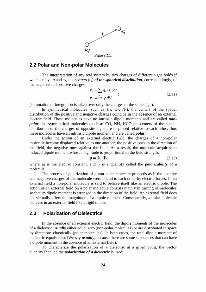
The Figure 2.2 shows schematically a polarized dielectric with non-polar (a) and

polar (b) molecules. The polarization is attended by the appearance of a surplus of

bound charges of the same sign in the thin surface layer of the dielectric.

Figure 2.2.

+- +- +- +-

+-

+-

+-

+-

+-

+-

+- +-

+- +-

+- +-

E E

+- +- +- +

-

+- +

- +- +-

+- +- +- +-

+- +- +

- +-

(a) (b)

26

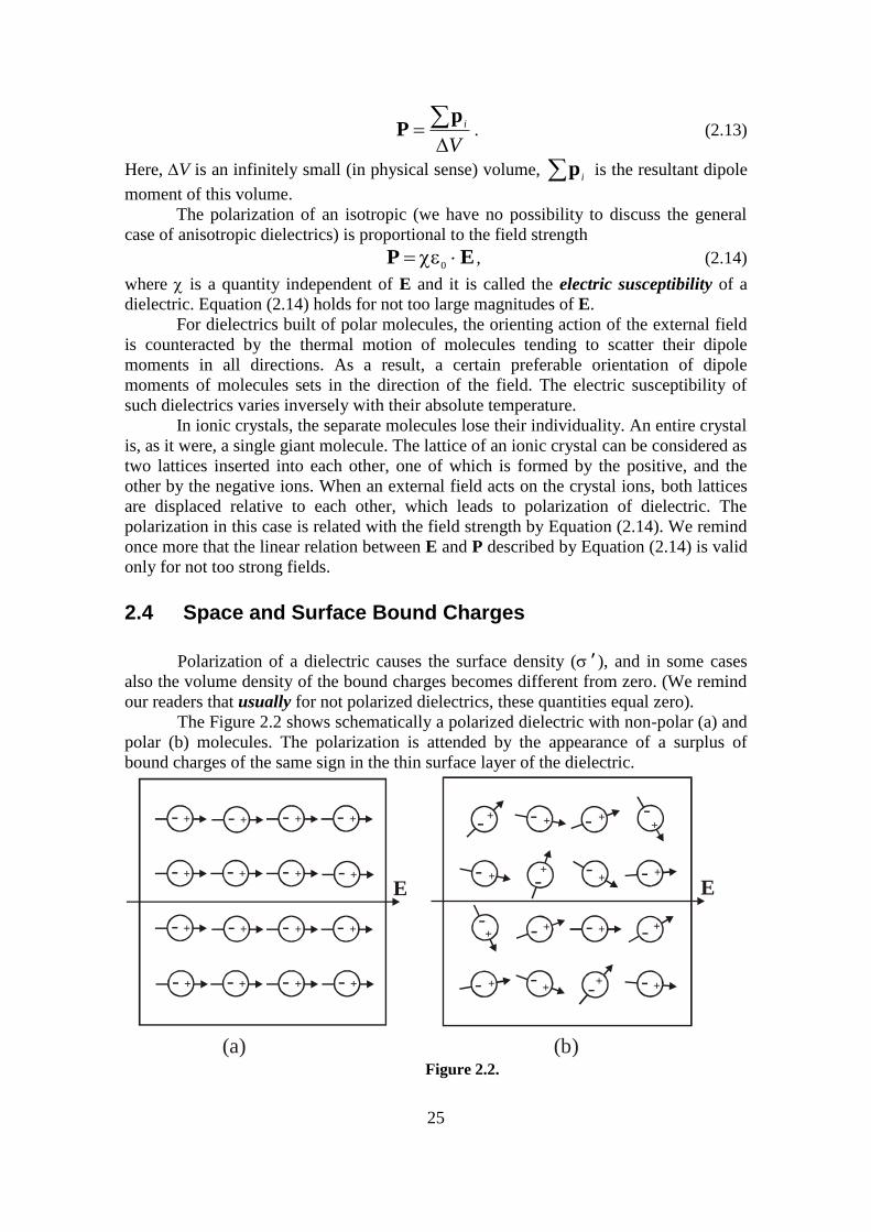
To find the relation between the polarization P and surface density of bound

charges ' , let us consider an infinite plane-parallel plate of a homogeneous dielectric

placed in a homogeneous electric field (see Figure 2.3).

Figure 2.3

Let us mentally separate an elementary volume in the plate in the form of a very

thin cylinder with generatrices parallel to E in the dielectric, and with bases of area S

coinciding with the surfaces of the plate. A dipole electric moment of this volume

cosSPlPdVp . (2.15)

On the other hand, it can be expressed as follows:

Slp . (2.16)

Comparing Equations (2.15) and (2.16) we conclude that

nPP cos , (2.17)

where Pn is the projection of polarization onto an outward normal to the relevant

surface. Using Equation (2.14) we can write Equation (2.17) as

nE

0 , (2.18)

where En is the normal component of the field strength inside the dielectric. According

to equation (2.18), at the points where the field lines emerge from the dielectric (En>0),

positive bound charges come up to the surface, while where the field lines enter the

dielectric (En<0), negative surface charges appear.

Equations (2.17) and (2.18) also hold in the most general case when an

inhomogeneous dielectric of an arbitrary shape is located in an inhomogeneous electric

field. By Pn and En we must understand now the normal component of the relevant

vector taken in direct proximity to the surface element for which ' is being determined.

Analogous but a little more tiresome calculations lead to the expression describing the

spatial density of bound charges:

P . (2.19)

I.e., the density of bound charges equals the divergence of the polarization vector P

taken with the opposite sign.

d

- ' '

l

P

E

n

S

+ q

( - S

- q

n

27

2.5 Electric Displacement Vector

Bound charges differ from extraneous ones only in that they cannot leave the

confines of the molecules which they are in. Otherwise, they have the same properties

as all other charges. In particular, they are the sources of an electric field. Therefore,

when the density of the bound charges ' differs from zero, equation (1.12) must be

written as follows:

)(1

0

E . (2.20)

Here, ' is the density of the extraneous charges. Equation (2.20) is of virtually no use

for finding the vector E because it expresses the properties of the unknown quantity E

through bound charges, which in turn are determined by the unknown quantity E.

Calculation of the fields is often simplified if we introduce an auxiliary quantity

whose source are only extraneous charges . To establish what this quantity looks like,

let us substitute equation (2.19) for ' into equation (2.20):

)(1

0

PE

, (2.21)

whence it follows that

)(0

PΕ . (2.22)

The quantity

PΕD 0 (2.23)

is called the electric displacement, it is just the required quantity. Inserting equation

(2.14) for P, we get

ΕΕΕD 1000 . (2.24)

The dimensionless quantity

1 (2.25)

is called the relative permittivity (or simply permittivity) of a medium. Thus,

ΕD 0

(2.26)

According the Equation (2.26), the vector D is proportional to the vector E. We remind

our readers that we are dealing with isotropic dielectrics. In anisotropic dielectrics, the

vectors E and D, generally speaking, are not collinear.

In accordance with Equations (1.7) and (2.26), the electric displacement of the

field of a point charge in a vacuum ( = 1) is

rr

qeD

24

1. (2.27)

Equation (2.22) can be written as

D . (2.28)

Integration of this Equation over an arbitrary volume V yields

V V

dVdVD , (2.29)

or

S V

dVSDd . (2.30)

28

The quantity on the left-hand side of (2.30) is D, the flux of the vector D through

closed surface S, while that on the right-hand side is the sum of the extraneous charges

iq enclosed by this surface. Hence,

iDq , (2.31)

Equation (2.31) is known to be the Gauss’ theorem for dielectric. This statement holds

also for any inhomogeneous dielectric.

The field of the vector D can be depicted with the aid of electric displacement

lines. Their direction and density are determined in exactly the same way as for the lines

of the vector E. The lines of vector E can begin and terminate at both extraneous and

bound charges. The sources of the field of the vector D are only extraneous charges.

Hence, displacement lines can begin or terminate only at extraneous charges. These

lines pass without interruption through points at which bound charges are placed.

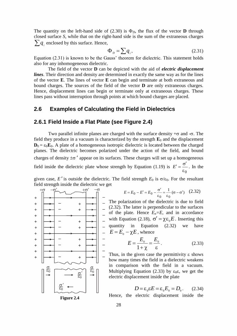
2.6 Examples of Calculating the Field in Dielectrics 2.6.1 Field Inside a Flat Plate (see Figure 2.4)

Two parallel infinite planes are charged with the surface density + and -. The

field they produce in a vacuum is characterized by the strength E0 and the displacement

D0 = E0. A plate of a homogeneous isotropic dielectric is located between the charged

planes. The dielectric becomes polarized under the action of the field, and bound

charges of density ' appear on its surfaces. These charges will set up a homogeneous

field inside the dielectric plate whose strength by Equation (1.19) is 0

E . In the

given case, E' is outside the dielectric. The field strength E0 is /0. For the resultant

field strength inside the dielectric we get

)(1

0000

EEEE (2.32)

The polarization of the dielectric is due to field

(2.32). The latter is perpendicular to the surfaces

of the plate. Hence En=E, and in accordance

with Equation (2.18), E0

. Inserting this

quantity in Equation (2.32) we have

EEE 0

, whence

00

1

EEE . (2.33)

Thus, in the given case the permittivity shows

how many times the field in a dielectric weakens

in comparison with the field in a vacuum.

Multiplying Equation (2.33) by , we get the

electric displacement inside the plate

0000DEED . (2.34)

Hence, the electric displacement inside the

''

_

_

_

_

_

_

_

_

_

_

_

_

_

_

_

_

_

_

_

+

+

+

+

+

+

+

+

+

+

+

+

+

+

+

+

+

+

0 0'

0

'0

Figure 2.4

29

dielectric coincides with that of the external field D0. Substituting /0 for E0 into

equation (2.34) we find

D =

To find ' , let us express E and E0 in Equation (2.32) through the charge densities:

00

0

0

)(1 E

E ,

whence

1. (2.36)

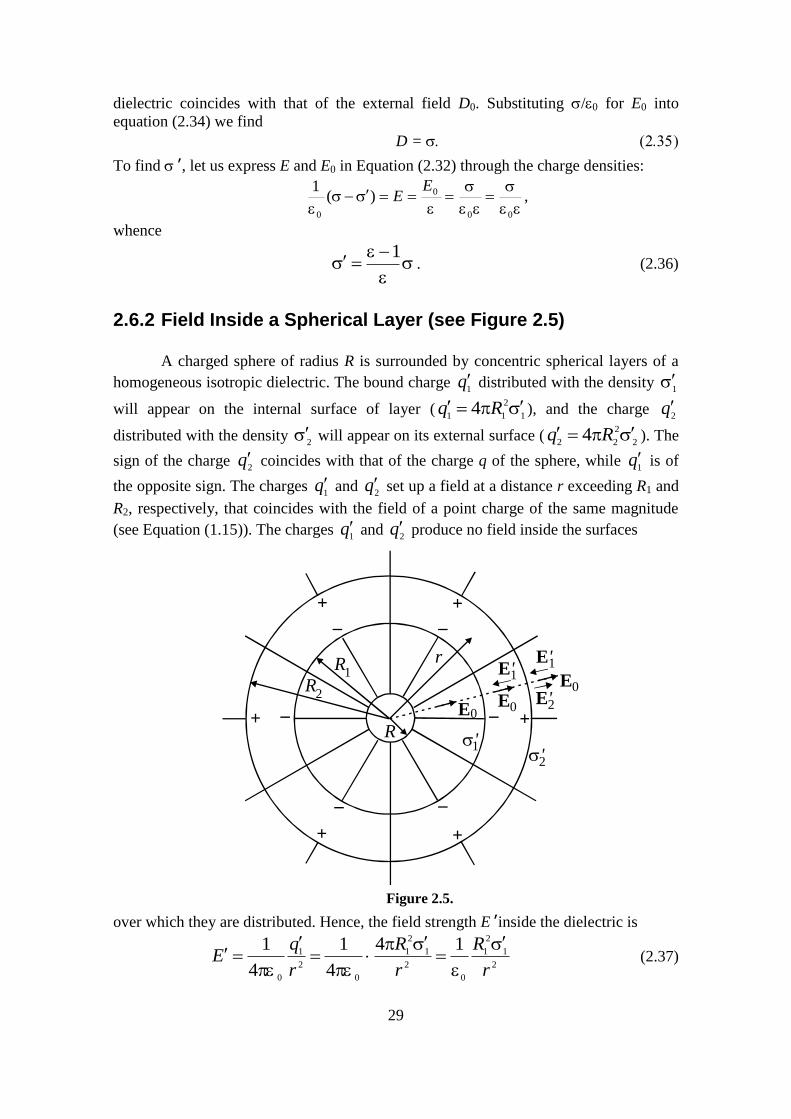
2.6.2 Field Inside a Spherical Layer (see Figure 2.5)

A charged sphere of radius R is surrounded by concentric spherical layers of a

homogeneous isotropic dielectric. The bound charge 1

q distributed with the density 1

will appear on the internal surface of layer (1

2

114 Rq ), and the charge

2q

distributed with the density 2

will appear on its external surface (2

2

224 Rq ). The

sign of the charge 2

q coincides with that of the charge q of the sphere, while 1

q is of

the opposite sign. The charges 1

q and 2

q set up a field at a distance r exceeding R1 and

R2, respectively, that coincides with the field of a point charge of the same magnitude

(see Equation (1.15)). The charges 1

q and 2

q produce no field inside the surfaces

Figure 2.5.

over which they are distributed. Hence, the field strength E' inside the dielectric is

2

1

2

1

0

2

1

2

1

0

2

1

0

14

4

1

4

1

r

R

r

R

r

qE

(2.37)

_

__

_

__

+

+

++

+

+

R

R

R1

2

r

''

1

2

E0

E0

E0E'

1

2

E'1E'

30

and is opposite in direction to the field strength E0. The resultant field inside the

dielectric

2

1

2

1

0

2

0

0

1

4

1)(

r

R

r

qEErE

. (2.38)

It diminishes in proportion to 1/r2. So, we can write

2

1

2

12

1

2

1 )()(or ,)(

)(

R

rrERE

R

r

rE

RE , (2.39)

where E(R1) is the field strength in the dielectric in direct proximity to the internal

surface of the layer. It is exactly the strength that determines the quantity 1

:

2

1

2

0101)()(

R

rrERE , (2.40)

(at each point of the surface |En|=E). Substituting expression for from equation (2.40)

into equation (2.38) we get

)()()(1

4

1)(

02

1

2

2

0

2

1

0

2

0

rErERr

rrER

r

qrE

, (2.41)

whence

)()( 0

rErE , (2.42)

000DED . (2.43)

The field inside the dielectric changes in proportion to 1/r2. Therefore, the

relation 2

1

2

221RR holds. Hence,

21qq . Consequently, the fields set up by

these charges at distances exceeding R2 mutually terminate each other so that outside

the spherical layer E'=0 and E=E0.

Assuming that R1=R and R2=, we arrive at the case of a charged sphere

immersed in an infinite homogeneous and isotropic dielectric. The field strength outside

such a sphere is

204

1

r

qE

. (2.44)

Both examples considered above are characterized by the fact that a dielectric

was homogeneous and isotropic, and the surfaces enclosing it coincided with the

equipotential surfaces of the field of extraneous charges. The result we have obtained in

these cases is a general one. If a homogeneous and isotropic dielectric completely fills

the volume enclosed by equipotential surfaces of the field of extraneous charges, then

the electric displacement vector coincides with the vector of the field strength of the

extraneous charges multiplied by 0, and therefore, the field strength inside the dielectric

is 1/ of that of the field strength of the extraneous charges in a vacuum.

If the above conditions are not satisfied, the vectors D and 0E do not coincide.

For example, Figure 2.6 shows the field in the dielectric plate skewed relative to the

planes carrying extraneous charges. The vector E' is perpendicular to the faces of the

plate, therefore E and E' are not collinear.

31

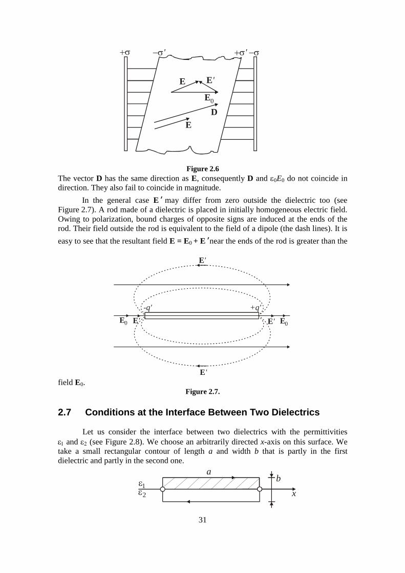
Figure 2.6

The vector D has the same direction as E, consequently D and 0E0 do not coincide in

direction. They also fail to coincide in magnitude.

In the general case E' may differ from zero outside the dielectric too (see

Figure 2.7). A rod made of a dielectric is placed in initially homogeneous electric field.

Owing to polarization, bound charges of opposite signs are induced at the ends of the

rod. Their field outside the rod is equivalent to the field of a dipole (the dash lines). It is

easy to see that the resultant field E = E0 + E' near the ends of the rod is greater than the

field E0. Figure 2.7.

2.7 Conditions at the Interface Between Two Dielectrics

Let us consider the interface between two dielectrics with the permittivities

and (see Figure 2.8). We choose an arbitrarily directed x-axis on this surface. We

take a small rectangular contour of length a and width b that is partly in the first

dielectric and partly in the second one.

''

E

D

E'

E

E

0

x

ba

1

2

+q'-q'

E'

E'

E' E' E0E0

32

Figure 2.8

Let E1 and E2 be the field strengths inside dielectrics. Since [E]=0, the circulation of

the vector E around the contour equals zero, i.e.

02,2,1

bEaEaEdlEbxxl

. (2.45)

where <Eb> is the mean value of El on the contour perpendicular to the interface. In the

limit, when the width b of the contour tends to zero, we get

E1,x = E2,x . (2.46)

Let us represent each of the vectors E1 and E2 as the sum of the normal and tangential

components:

E1 = E1,n + E1, E2 = E2,n + E2,

The equation (2.46) signifies that

E1, = E2,

Substituting the projections of the vector D divided by for the projections of the

vector E, we get

20

,2

10

,1

DD

,

(2.49)

whence it follows that

2

1

,2

,1

D

D. (2.50)

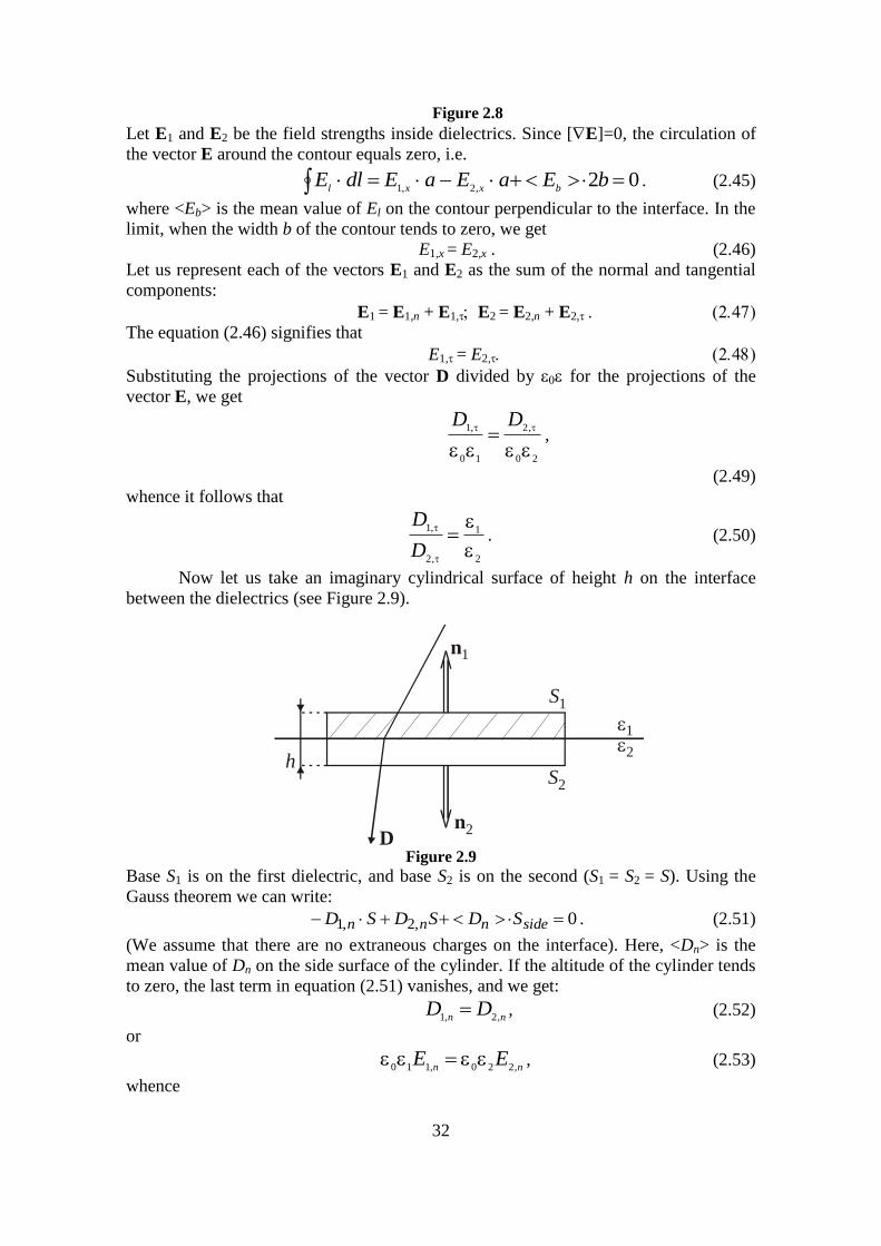
Now let us take an imaginary cylindrical surface of height h on the interface

between the dielectrics (see Figure 2.9).

Figure 2.9

Base S1 is on the first dielectric, and base S2 is on the second (S1 = S2 = S). Using the

Gauss theorem we can write:

0,2,1 sidennn SDSDSD . (2.51)

(We assume that there are no extraneous charges on the interface). Here, <Dn> is the

mean value of Dn on the side surface of the cylinder. If the altitude of the cylinder tends

to zero, the last term in equation (2.51) vanishes, and we get:

nnDD

,2,1 , (2.52)

or

nnEE

,220,110 , (2.53)

whence

h

1

2

S1

S2

n

n

1

2D

33

1

2

,2

.1

n

n

E

E. (2.54)

The results we have obtained signify that when passing through the interface

between two dielectrics, the normal component of the vector D and the tangential

component of the vector E change continuously. The tangential component of the vector

D and the normal component of the vector E, however, are disrupted when passing

through the interface.

Equations (2.48), (2.50), (2.52), and (2.54) determine the conditions which the

vector E and D must comply with on the interface between two dielectrics (if there are

no extraneous charges on this interface). We have obtained these equations for an

electrostatic field. They also hold, however, for fields varying in time.

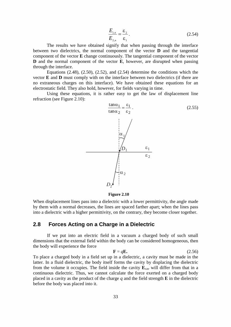
Using these equations, it is rather easy to get the law of displacement line

refraction (see Figure 2.10):

2

1

2

1

tan

tan

. (2.55)

When displacement lines pass into a dielectric with a lower permittivity, the angle made

by them with a normal decreases, the lines are spaced farther apart; when the lines pass

into a dielectric with a higher permittivity, on the contrary, they become closer together.

2.8 Forces Acting on a Charge in a Dielectric

If we put into an electric field in a vacuum a charged body of such small

dimensions that the external field within the body can be considered homogeneous, then

the body will experience the force

F = qE. (2.56)

To place a charged body in a field set up in a dielectric, a cavity must be made in the

latter. In a fluid dielectric, the body itself forms the cavity by displacing the dielectric

from the volume it occupies. The field inside the cavity Ecav will differ from that in a

continuous dielectric. Thus, we cannot calculate the force exerted on a charged body

placed in a cavity as the product of the charge q and the field strength E in the dielectric

before the body was placed into it.

D

1

2

2

2

11

Figure 2.10

34

When calculating the force acting on a charged body in a fluid dielectric, the

mechanical tension Ften set up on the boundary with the body must be taken into

account.

Thus, the force acting on a charged body in a dielectric, generally speaking,

cannot be determined by equation (2.56), and it is usually a very complicated task to

calculate it. These calculations give an interesting result for a fluid dielectric. The

resultant of the electric force qEcav and the mechanical force Ften is found to be exactly

equal to qE, where E is the field strength in the continuous dielectric

EFEF qq tencav . (2.57)

The strength of the field produced in a homogeneous infinitely extending

dielectric by a point charge is determined by equation (2.44). Hence, we get the

following expression for the force of interaction of two point charges immersed in a

homogeneous infinitely extending fluid dielectric

221

04

1

r

qqF

. (2.58)

Some authors characterize equation (2.58) as “the most general expression of

Coulomb’s law”. In this connection, we are going to cite Richard P. Feynman: “Many

older books on electricity start with the “fundamental” law that the force between two

charges is …[equation (2.58) is given]…, a point of view is thoroughly unsatisfactory.

For one thing, it is not true in general; it is true only for a world filled with a liquid.

Secondly, it depends on the fact that is a constant which is only approximately true for

most real materials”.

In this textbook, we are not going to discuss problems relating to the forces

acting on a charge inside a cavity made in a solid dielectric.

Examples

Problem 1 A parallel-plate capacitor has a capacitance C0 in the absence of dielectric. A slab

of dielectric material of dielectric constant

and thickness d/3 is inserted between the

plates (Fig.15). What is the new capacitance

when the dielectric is present?

Reasoning: This capacitor is equivalent of

two parallel-plate capacitors of the same area

A connected in series, one (C1) with a plate separation d/3 (dielectric filled) and the

other (C2) with a plate separation 2d/3 and air between the plates (Figure 15) The two

capacitances are

3

01

d

AC

and

32

01

d

AC

.

Solution Using the equation for two capacitors combined in series, we get

Figure 15

A parallel-plate capacitor of plate separation d

partially filled with a dielectric of thickness

d/3

d

13

32

_

_

d

d

35

21

32

1

3

323111

000021 A

d

A

d

A

d

A

d

CCC,

d

AC 0

12

3

.

Since the capacitance without the dielectric is C0 = 0A/d, we see that

012

3CC

.

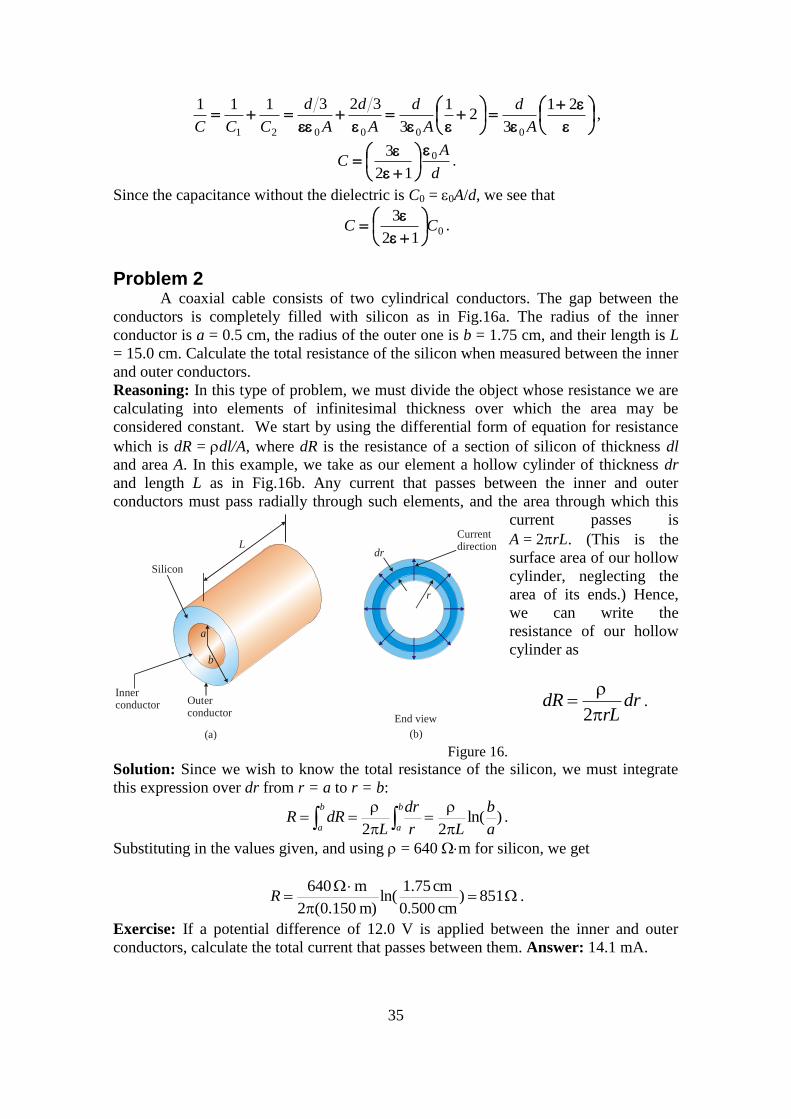
Problem 2 A coaxial cable consists of two cylindrical conductors. The gap between the

conductors is completely filled with silicon as in Fig.16a. The radius of the inner

conductor is a = 0.5 cm, the radius of the outer one is b = 1.75 cm, and their length is L

= 15.0 cm. Calculate the total resistance of the silicon when measured between the inner

and outer conductors.

Reasoning: In this type of problem, we must divide the object whose resistance we are

calculating into elements of infinitesimal thickness over which the area may be

considered constant. We start by using the differential form of equation for resistance

which is dR = dl/A, where dR is the resistance of a section of silicon of thickness dl

and area A. In this example, we take as our element a hollow cylinder of thickness dr

and length L as in Fig.16b. Any current that passes between the inner and outer

conductors must pass radially through such elements, and the area through which this

current passes is

A = 2rL. (This is the

surface area of our hollow

cylinder, neglecting the

area of its ends.) Hence,

we can write the

resistance of our hollow

cylinder as

drrL

dR

2.

Figure 16.

Solution: Since we wish to know the total resistance of the silicon, we must integrate

this expression over dr from r = a to r = b:

)ln(22 a

b

Lr

dr

LdRR

b

a

b

a

.

Substituting in the values given, and using = 640 m for silicon, we get

851)

cm 500.0

cm 75.1ln(

m)150.0(2

m 640R .

Exercise: If a potential difference of 12.0 V is applied between the inner and outer

conductors, calculate the total current that passes between them. Answer: 14.1 mA.

L

a

b

Silicon

Innerconductor Outer

conductor

(a)

dr

r

Current direction

(b)

End view

36

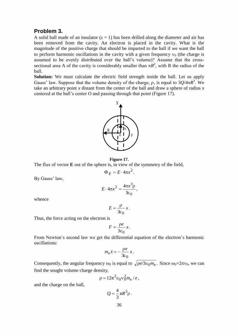
Problem 3. A solid ball made of an insulator (= 1) has been drilled along the diameter and air has

been removed from the cavity. An electron is placed in the cavity. What is the

magnitude of the positive charge that should be imparted to the ball if we want the ball

to perform harmonic oscillations in the cavity with a given frequency 0 (the charge is

assumed to be evenly distributed over the ball’s volume)? Assume that the cross-

sectional area A of the cavity is considerably smaller than R2, with R the radius of the

ball.

Solution: We must calculate the electric field strength inside the ball. Let us apply

Gauss’ law. Suppose that the volume density of the charge, , is equal to 3Q/4R3. We

take an arbitrary point x distant from the center of the ball and draw a sphere of radius x

centered at the ball’s center O and passing through that point (Figure 17).

Figure 17.

The flux of vector E out of the sphere is, in view of the symmetry of the field, 24 xEE .

By Gauss’ law,

0

32

3

44

xxE ,

whence

xE03

.

Thus, the force acting on the electron is

xe

F03ε

ρ .

From Newton’s second law we get the differential equation of the electron’s harmonic

oscillations:

xe

xm0

e3

.

Consequently, the angular frequency 0 is equal to ./3ερ e0me Since 0=2, we can

find the sought volume charge density,

em /ε12πρ e200

2 ,

and the charge on the ball,

ρπ3

4 3RQ .

xR

X

o

37

For

Hz = 1 Mhz and R = 10-1

m we have 610-9

C/m3 and Q 2.410

-11 C.

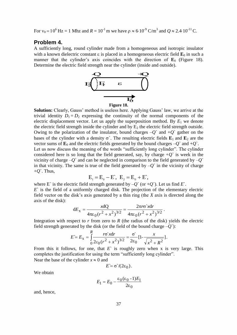
Problem 4. A sufficiently long, round cylinder made from a homogeneous and isotropic insulator

with a known dielectric constant is placed in a homogeneous electric field E0 in such a

manner that the cylinder’s axis coincides with the direction of E0 (Figure 18).

Determine the electric field strength near the cylinder (inside and outside).

Figure 18.

Solution: Clearly, Gauss’ method is useless here. Applying Gauss’ law, we arrive at the

trivial identity D1 = D2 expressing the continuity of the normal components of the

electric displacement vector. Let us apply the superposition method. By E1 we denote

the electric field strength inside the cylinder and by E2 the electric field strength outside.

Owing to the polarization of the insulator, bound charges –Q` and +Q` gather on the

bases of the cylinder with a density `. The resulting electric fields E1 and E2 are the

vector sums of E0 and the electric fields generated by the bound charges –Q` and +Q`.

Let us now discuss the meaning of the words “sufficiently long cylinder”. The cylinder

considered here is so long that the field generated, say, by charge +Q` is week in the

vicinity of charge –Q` and can be neglected in comparison to the field generated by –Q`

in that vicinity. The same is true of the field generated by –Q` in the vicinity of charge

+Q`. Thus,

E ,̀EE E ,̀EE0201

where E` is the electric field strength generated by –Q` (or +Q`). Let us find E`.

E` is the field of a uniformly charged disk. The projection of the elementary electric

field vector on the disk’s axis generated by a thin ring (the X axis is directed along the

axis of the disk):

3/2220

3/2220

x)(4

d`2

)(4

dQd

xr

rxr

xr

xE

.

Integration with respect to r from zero to R (the radius of the disk) yields the electric

field strength generated by the disk (or the field of the bound charge –Q`):

]1[2ε

σ`

)(2

dσ``

22003/222

0

x

Rx

x-

xrε

rxrEE

R

.

From this it follows, for one, that E` is roughly zero when x is very large. This

completes the justification for using the term “sufficiently long cylinder”.

Near the base of the cylinder x 0 and

)2ε`/(σ` 0E .

We obtain

0

10001

2

1)-(

EEE

and, hence,

EE

-Q̀ +Q̀

E

2 1

0

38

011

2EE

.

Then, it yields

001

1-2` E

.

We obtain

01

1-` EE

.

Hence,

02ε1

2εEE

.

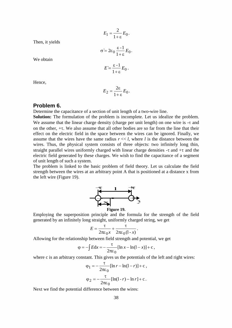
Problem 6. Determine the capacitance of a section of unit length of a two-wire line.

Solution: The formulation of the problem is incomplete. Let us idealize the problem.

We assume that the linear charge density (charge per unit length) on one wire is - and

on the other, +. We also assume that all other bodies are so far from the line that their

effect on the electric field in the space between the wires can be ignored. Finally, we

assume that the wires have the same radius r << l, where l is the distance between the

wires. Thus, the physical system consists of three objects: two infinitely long thin,

straight parallel wires uniformly charged with linear charge densities -and + and the

electric field generated by these charges. We wish to find the capacitance of a segment

of unit length of such a system.

The problem is linked to the basic problem of field theory. Let us calculate the field

strength between the wires at an arbitrary point A that is positioned at a distance x from

the left wire (Figure 19).

Figure 19.

Employing the superposition principle and the formula for the strength of the field

generated by an infinitely long straight, uniformly charged string, we get

)-(l22 00 xxE

.

Allowing for the relationship between field strength and potential, we get

c)](lln[ln2

d0

xxxE ,

where c is an arbitrary constant. This gives us the potentials of the left and right wires:

c)](lln[ln2 0

1

rr ,

c]ln)-l[ln(2 0

2

rr .

Next we find the potential difference between the wires:

._ +

l

x X

+

39

r

r-lln

021

.

Since r<<l by hypothesis, we have

.l

ln0 r

Employing relationship C = Q/, we can determine the capacitance of a section of unit

length of a two-wire line:

.)ln(l/

C 0

r

3. Steady Electric Current 3.1 Electric Current

If a total charge other than zero is carried through a surface, an electric current

(or simply current) is said to flow through this surface. For a current to flow, the given

medium must contain charged particles that can move in the limits of the medium. Such

particles are called current carriers (electrons, ions, or even macroscopic particles). A

current is produced if there is an electric field inside the body. The mean value of the

velocity of thermal motion is zero, thus when the electric field acts upon the current

carriers, they acquire the additional velocity U coinciding for the positive carriers with

the field direction and opposite to that for the negative carriers. If the charge dq is

carried through a surface during the time dt, it is said the current strength (or simply

the current)

dt

dqI (3.1)

is established. The transfer of a negative charge in one direction is equivalent to the

transfer of a positive charge of the same magnitude in the opposite direction. Thus, if a

current is produced by carriers of both signs, we can write

dt

dq

dt

dqI

. (3.2)

The direction of motion of the positive carriers has been historically assumed to be the

direction of a current.

A current (I) is a scalar quantity and it can be distributed non-uniformly over the

relevant surface. In order to characterize this distribution, a vector quantity j, called the

current density is introduced

Sj ddI . (3.3)

Thus, the current flowing through the elementary surface characterized by the surface

vector dS can be expressed as a scalar product of j and dS.

Let us assume that the space densities of positive and negative charges are,

correspondingly, n+ and n

-. If the carriers acquire the average velocities U

+ and U

-, then

the current density can be expressed as: UUj nene . (3.4)

In equation (3.4) both addends are of the same direction: the vector U- is directed

oppositely to the vector j, when it is multiplied by the negative scalar e-, we get a vector

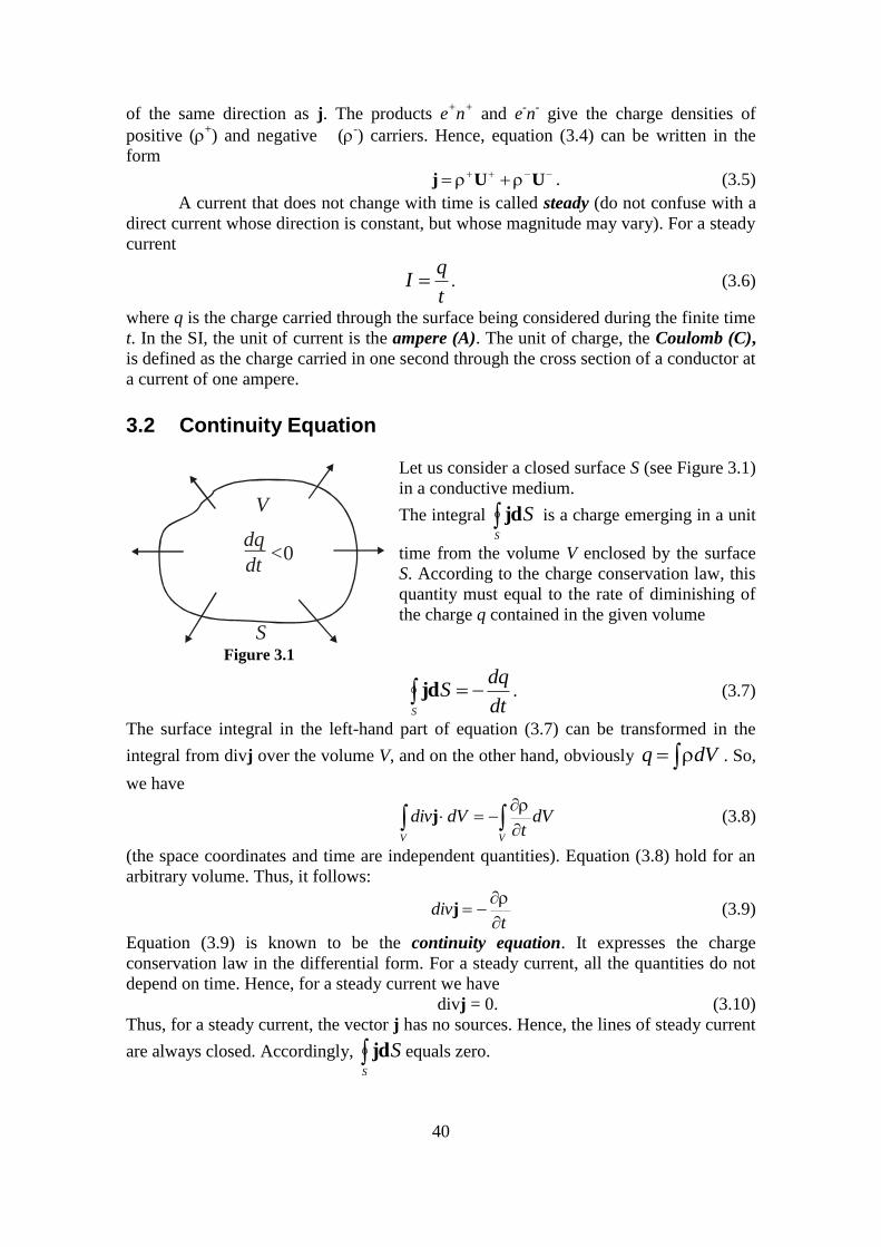
40

of the same direction as j. The products e+n

+ and e

-n

- give the charge densities of

positive (+) and negative (

-) carriers. Hence, equation (3.4) can be written in the

form UUj . (3.5)

A current that does not change with time is called steady (do not confuse with a

direct current whose direction is constant, but whose magnitude may vary). For a steady

current

t

qI . (3.6)

where q is the charge carried through the surface being considered during the finite time

t. In the SI, the unit of current is the ampere (A). The unit of charge, the Coulomb (C),

is defined as the charge carried in one second through the cross section of a conductor at

a current of one ampere.

3.2 Continuity Equation

Let us consider a closed surface S (see Figure 3.1)

in a conductive medium.

The integral S

Sjd is a charge emerging in a unit

time from the volume V enclosed by the surface

S. According to the charge conservation law, this

quantity must equal to the rate of diminishing of

the charge q contained in the given volume

Figure 3.1

S dt

dqSjd . (3.7)

The surface integral in the left-hand part of equation (3.7) can be transformed in the

integral from divj over the volume V, and on the other hand, obviously dVq . So,

we have

VV

dVt

dVdivj (3.8)

(the space coordinates and time are independent quantities). Equation (3.8) hold for an

arbitrary volume. Thus, it follows:

tdiv

j (3.9)

Equation (3.9) is known to be the continuity equation. It expresses the charge

conservation law in the differential form. For a steady current, all the quantities do not

depend on time. Hence, for a steady current we have

divj = 0. (3.10)

Thus, for a steady current, the vector j has no sources. Hence, the lines of steady current

are always closed. Accordingly, S

Sjd equals zero.

V

S

dq__dt

<0

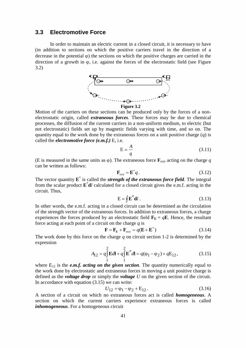
41

3.3 Electromotive Force

In order to maintain an electric current in a closed circuit, it is necessary to have

(in addition to sections on which the positive carriers travel in the direction of a

decrease in the potential ) the sections on which the positive charges are carried in the

direction of a growth in , i.e. against the forces of the electrostatic field (see Figure

3.2)

Figure 3.2

Motion of the carriers on these sections can be produced only by the forces of a non-

electrostatic origin, called extraneous forces. These forces may be due to chemical

processes, the diffusion of the current carriers in a non-uniform medium, to electric (but

not electrostatic) fields set up by magnetic fields varying with time, and so on. The

quantity equal to the work done by the extraneous forces on a unit positive charge (q) is

called the electromotive force (e.m.f.) E, i.e.

q

A (3.11)

(E is measured in the same units as ). The extraneous force Fextr acting on the charge q

can be written as follows:

q*

extr EF . (3.12)

The vector quantity E* is called the strength of the extraneous force field. The integral

from the scalar product E*dl calculated for a closed circuit gives the e.m.f. acting in the

circuit. Thus,

ldE*E . (3.13)

In other words, the e.m.f. acting in a closed circuit can be determined as the circulation

of the strength vector of the extraneous forces. In addition to extraneous forces, a charge

experiences the forces produced by an electrostatic field FE = qE. Hence, the resultant

force acting at each point of a circuit on the charge q is

)( *

extr EEFFF E q (3.14)

The work done by this force on the charge q on circuit section 1-2 is determined by the

expression

1221

2

1

*2

1

12 E)( qqdqdqA lElE , (3.15)

where E12 is the e.m.f. acting on the given section. The quantity numerically equal to

the work done by electrostatic and extraneous forces in moving a unit positive charge is

defined as the voltage drop or simply the voltage U on the given section of the circuit.

In accordance with equation (3.15) we can write:

122112 EU . (3.16)

A section of a circuit on which no extraneous forces act is called homogeneous. A

section on which the current carriers experience extraneous forces is called

inhomogeneous. For a homogeneous circuit

+

+ + +

+

+

1 2

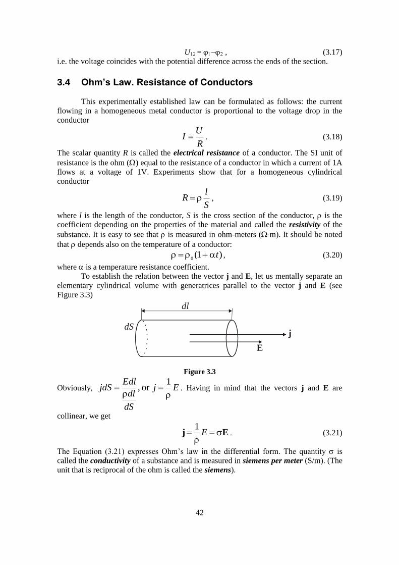
42

U12 = , (3.17)

i.e. the voltage coincides with the potential difference across the ends of the section.

3.4 Ohm’s Law. Resistance of Conductors

This experimentally established law can be formulated as follows: the current

flowing in a homogeneous metal conductor is proportional to the voltage drop in the

conductor

R

UI . (3.18)

The scalar quantity R is called the electrical resistance of a conductor. The SI unit of

resistance is the ohm () equal to the resistance of a conductor in which a current of 1A

flows at a voltage of 1V. Experiments show that for a homogeneous cylindrical

conductor

S

lR , (3.19)

where l is the length of the conductor, S is the cross section of the conductor, is the

coefficient depending on the properties of the material and called the resistivity of the

substance. It is easy to see that is measured in ohm-meters (m). It should be noted

that depends also on the temperature of a conductor:

)1(0

t , (3.20)

where is a temperature resistance coefficient.

To establish the relation between the vector j and E, let us mentally separate an

elementary cylindrical volume with generatrices parallel to the vector j and E (see

Figure 3.3)

Figure 3.3

Obviously, Ej

dS

dl

EdljdS

1or , . Having in mind that the vectors j and E are

collinear, we get

Ej

E1

. (3.21)

The Equation (3.21) expresses Ohm’s law in the differential form. The quantity is

called the conductivity of a substance and is measured in siemens per meter (S/m). (The

unit that is reciprocal of the ohm is called the siemens).

dS

dl

E

j

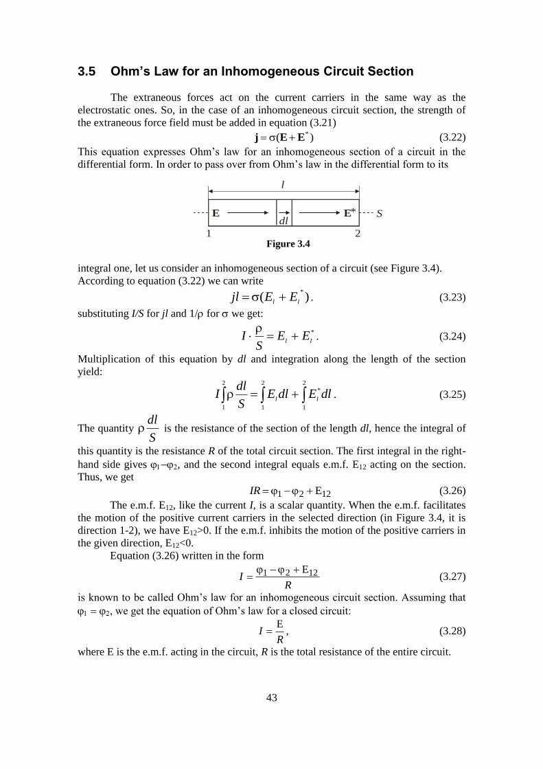
43

3.5 Ohm’s Law for an Inhomogeneous Circuit Section

The extraneous forces act on the current carriers in the same way as the

electrostatic ones. So, in the case of an inhomogeneous circuit section, the strength of

the extraneous force field must be added in equation (3.21)

)( *EEj (3.22)

This equation expresses Ohm’s law for an inhomogeneous section of a circuit in the

differential form. In order to pass over from Ohm’s law in the differential form to its

Figure 3.4

integral one, let us consider an inhomogeneous section of a circuit (see Figure 3.4).

According to equation (3.22) we can write

)(*

llEEjl . (3.23)

substituting I/S for jl and 1/ for we get:

*

llEE

SI

. (3.24)

Multiplication of this equation by dl and integration along the length of the section

yield:

2

1

*

2

1

2

1

dlEdlES

dlI

ll. (3.25)

The quantity S

dl is the resistance of the section of the length dl, hence the integral of

this quantity is the resistance R of the total circuit section. The first integral in the right-

hand side gives , and the second integral equals e.m.f. E12 acting on the section.

Thus, we get

1221 EIR (3.26)

The e.m.f. E12, like the current I, is a scalar quantity. When the e.m.f. facilitates

the motion of the positive current carriers in the selected direction (in Figure 3.4, it is

direction 1-2), we have E12>0. If the e.m.f. inhibits the motion of the positive carriers in

the given direction, E12<0.

Equation (3.26) written in the form

RI 1221 E (3.27)

is known to be called Ohm’s law for an inhomogeneous circuit section. Assuming that

, we get the equation of Ohm’s law for a closed circuit:

RI

E , (3.28)

where E is the e.m.f. acting in the circuit, R is the total resistance of the entire circuit.

l

E E*

1 2

Sdl

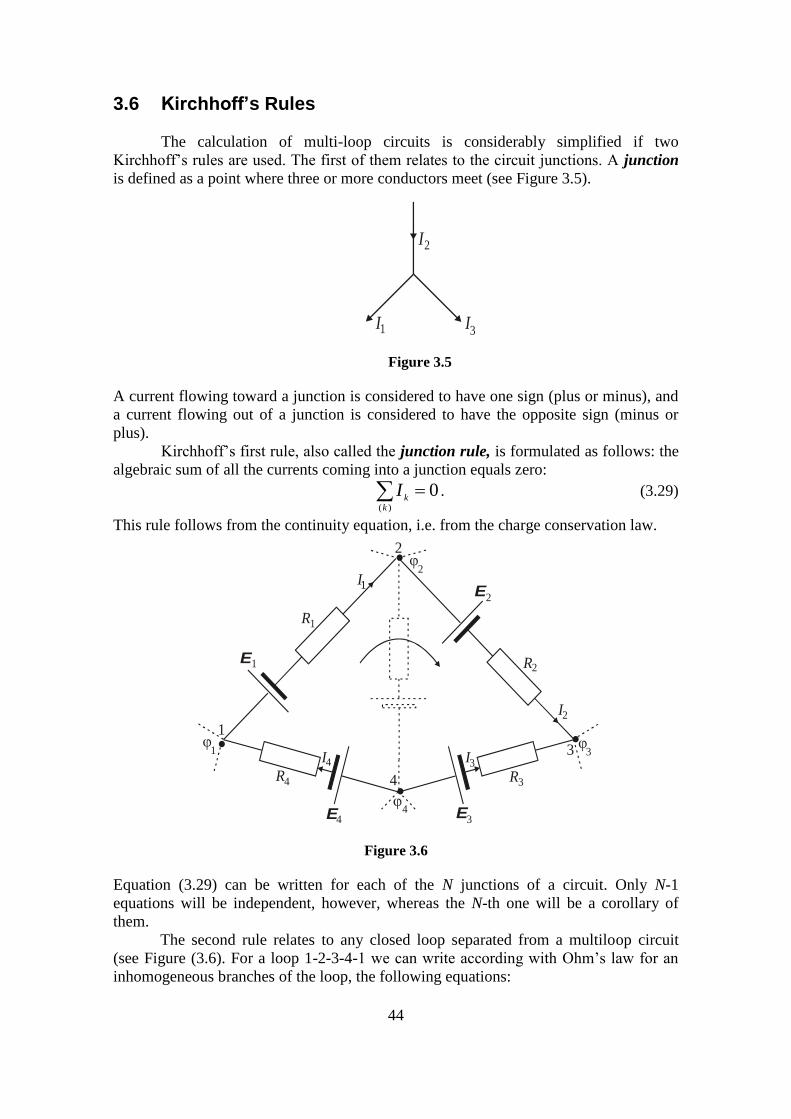
44

3.6 Kirchhoff’s Rules

The calculation of multi-loop circuits is considerably simplified if two

Kirchhoff’s rules are used. The first of them relates to the circuit junctions. A junction

is defined as a point where three or more conductors meet (see Figure 3.5).

Figure 3.5

A current flowing toward a junction is considered to have one sign (plus or minus), and

a current flowing out of a junction is considered to have the opposite sign (minus or

plus).

Kirchhoff’s first rule, also called the junction rule, is formulated as follows: the

algebraic sum of all the currents coming into a junction equals zero:

0)(

k

kI . (3.29)

This rule follows from the continuity equation, i.e. from the charge conservation law.

Figure 3.6

Equation (3.29) can be written for each of the N junctions of a circuit. Only N-1

equations will be independent, however, whereas the N-th one will be a corollary of

them.

The second rule relates to any closed loop separated from a multiloop circuit

(see Figure (3.6). For a loop 1-2-3-4-1 we can write according with Ohm’s law for an

inhomogeneous branches of the loop, the following equations:

I

1

2

3I I

1

2

3

4

.

...1

2

3

4

1

R

R2

RR 34

I

I

I

I

1

2

34

E

E

E E

1

1

3

2

4

45

41444

34333

23222

12111

E

E

E

E

RI

RI

RI

RI

When these expressions are summed, the potentials are cancelled, and we get

k

Ekk

RI (3.30)

Equation (3.30) expresses Kirchhoff’s second rule, also called the loop rule. Equation

(3.30) can be written for all the closed loops that can be separated mentally in a given

multiloop circuit. Only the equations for the loop that cannot be obtained by the

superposition of the loops on one another will be independent, however.

3.7 Power of a Current

The electrostatic and extraneous forces acting on the given section of an electric

circuit do the work

UItUqA . (3.31)

Dividing equation (3.31) by the time t during which it is done we get the power of the

current

IIUIP1221

)( E . (3.32)

The ratio of the power P developed by a current in the volume V of a

conductor to the magnitude of this volume is called the unit power of the current PU

corresponding to the given point of the conductor

V

PP

U

. (3.33)

An expression for the unit power can be obtained from the following

considerations. The force e(E+E*) develops a power of

UEE )( * eP , (3.34)

where U is the average velocity of the carriers (the thermal velocity must be taken into

consideration!).

Obviously, the power P developed in the volume V can be obtained by

multiplying P' by the number of current carriers in this volume, i.e. by nV (n is the

number of carriers per unit volume). Thus,

VVneP * )()( *EEjUEE . (3.35)

Hence,

)( *EEj

UP . (3.36)

This expression is a differential form of the integral equation (3.32).

3.8 The Joule-Lenz Law

When a conductor is stationary and no chemical transformations occur in it, the

work done by current increases the internal energy of the conductor, and as a result the

latter gets heated, i.e. the heat

UItQ (3.37)

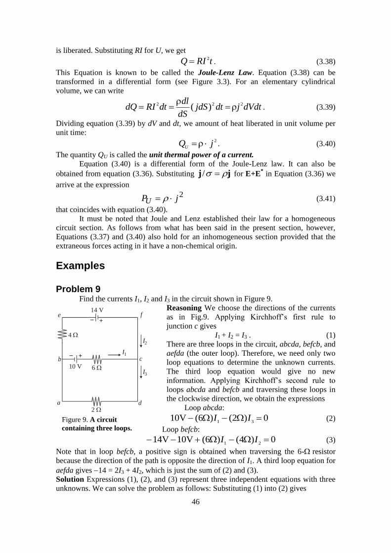
46

is liberated. Substituting RI for U, we get

tRIQ 2 . (3.38)

This Equation is known to be called the Joule-Lenz Law. Equation (3.38) can be

transformed in a differential form (see Figure 3.3). For an elementary cylindrical

volume, we can write

dVdtjdtjdSdS

dldtRIdQ 222 )(

. (3.39)

Dividing equation (3.39) by dV and dt, we amount of heat liberated in unit volume per

unit time: 2jQ

U . (3.40)

The quantity QU is called the unit thermal power of a current.

Equation (3.40) is a differential form of the Joule-Lenz law. It can also be

obtained from equation (3.36). Substituting jj / for E+E* in Equation (3.36) we

arrive at the expression

2jPU (3.41)

that coincides with equation (3.40).

It must be noted that Joule and Lenz established their law for a homogeneous

circuit section. As follows from what has been said in the present section, however,

Equations (3.37) and (3.40) also hold for an inhomogeneous section provided that the

extraneous forces acting in it have a non-chemical origin.

Examples Problem 9 Find the currents I1, I2 and I3 in the circuit shown in Figure 9.

Reasoning We choose the directions of the currents

as in Fig.9. Applying Kirchhoff’s first rule to

junction c gives

I1 + I2 = I3 . (1)

There are three loops in the circuit, abcda, befcb, and

aefda (the outer loop). Therefore, we need only two

loop equations to determine the unknown currents.

The third loop equation would give no new

information. Applying Kirchhoff’s second rule to

loops abcda and befcb and traversing these loops in

the clockwise direction, we obtain the expressions

Loop abcda:

0)2()6(V1031 II (2)

Loop befcb:

0)4()6(V10V1421 II (3)

Note that in loop befcb, a positive sign is obtained when traversing the 6-resistor

because the direction of the path is opposite the direction of I1. A third loop equation for

aefda gives 14 = 2I3 + 4I2, which is just the sum of (2) and (3).

Solution Expressions (1), (2), and (3) represent three independent equations with three

unknowns. We can solve the problem as follows: Substituting (1) into (2) gives

Figure 9. A circuit

containing three loops.

e f14 V_

+

4

b10 V

_+

6

I1

I2

c

I3

2 a d

47

10 6I1 2(I1 I2) = 0;

10 = 8I1 + 2I2. (4)

Dividing each term in (3) by 2 and rearranging the equation gives

12 = 3I1 + 2I2. (5)

Subtracting (5) from (4) eliminates I2, giving

22 = 11I1;

I1 = 2A.

Using this value of I1 in (5) gives a value for I2:

2I2 = 3I1 12 = 3(2) 12 = 6;

I2 = 3A.

Finally, I3 = I1 + I2 = 1A. Hence, the currents have the values

I1 = 2A I2 = -3A I3 = -1A

The fact that I2 and I3 are both negative indicates only that we chose the wrong direction

for these currents. However, the numerical values are correct.

Exercise: Find the potential difference between points b and c.

Answer: Vb Vc = 2V.

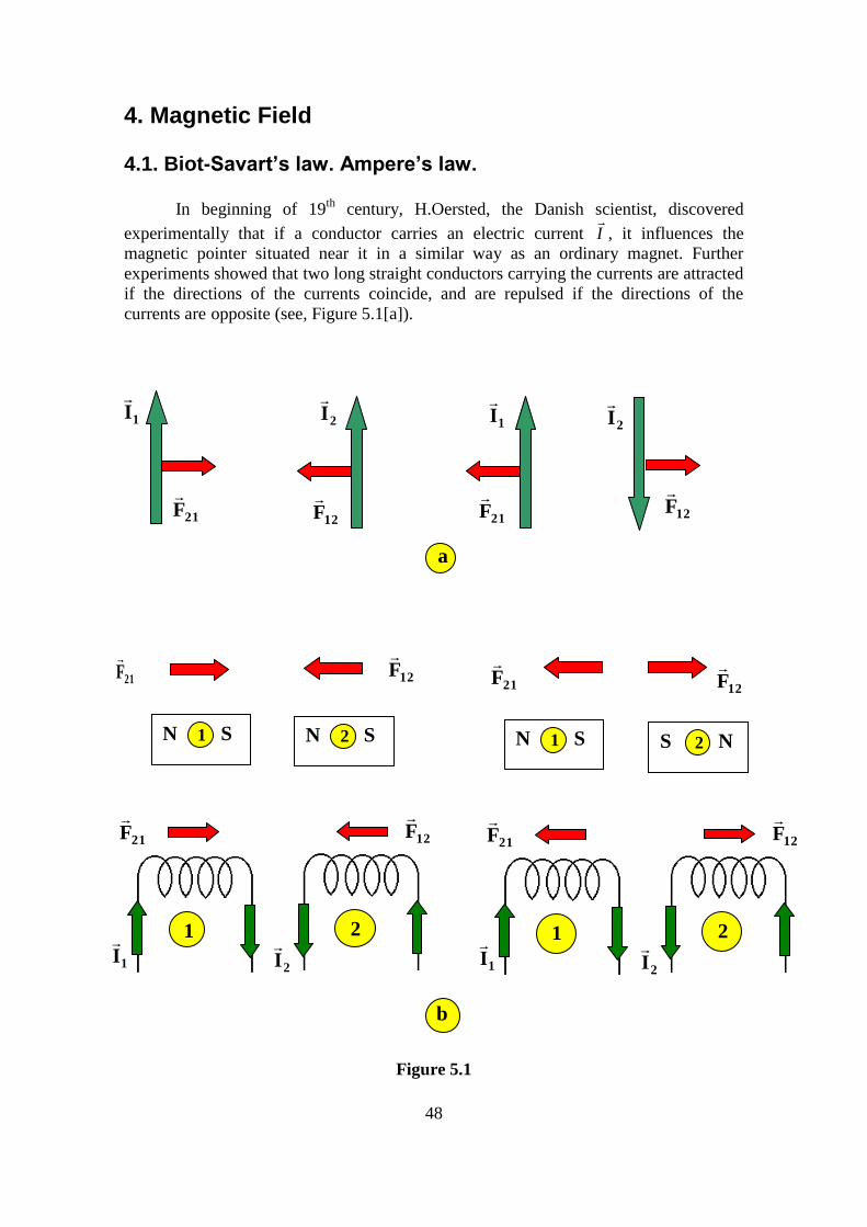
48

4. Magnetic Field

4.1. Biot-Savart’s law. Ampere’s law.

In beginning of 19th

century, H.Oersted, the Danish scientist, discovered

experimentally that if a conductor carries an electric current I

, it influences the

magnetic pointer situated near it in a similar way as an ordinary magnet. Further

experiments showed that two long straight conductors carrying the currents are attracted

if the directions of the currents coincide, and are repulsed if the directions of the

currents are opposite (see, Figure 5.1[a]).

12F

Figure 5.1

a

1I

21F

2I

12F

21F

1I

2I

12F

b

N S 1 N S 1 N S 2 S N 2

21F

12F

21F

21F

1I

1

12F

2

2I

21F

1I

1

12F

2

2I

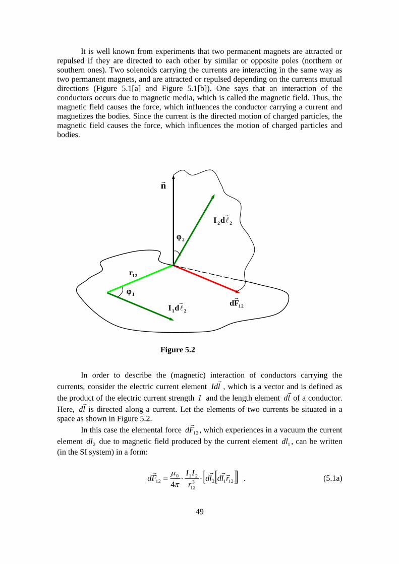
49

It is well known from experiments that two permanent magnets are attracted or

repulsed if they are directed to each other by similar or opposite poles (northern or

southern ones). Two solenoids carrying the currents are interacting in the same way as

two permanent magnets, and are attracted or repulsed depending on the currents mutual

directions (Figure 5.1[a] and Figure 5.1[b]). One says that an interaction of the

conductors occurs due to magnetic media, which is called the magnetic field. Thus, the

magnetic field causes the force, which influences the conductor carrying a current and

magnetizes the bodies. Since the current is the directed motion of charged particles, the

magnetic field causes the force, which influences the motion of charged particles and

bodies.

In order to describe the (magnetic) interaction of conductors carrying the

currents, consider the electric current element lId

, which is a vector and is defined as

the product of the electric current strength I and the length element ld

of a conductor.

Here, ld

is directed along a current. Let the elements of two currents be situated in a

space as shown in Figure 5.2.

In this case the elemental force 12Fd

, which experiences in a vacuum the current

element 2dl due to magnetic field produced by the current element 1dl , can be written

(in the SI system) in a form:

12123

12

210

124

rldldr

IIFd

. (5.1a)

Figure 5.2

n

2

12Fd

22dI

12r

21dI

1

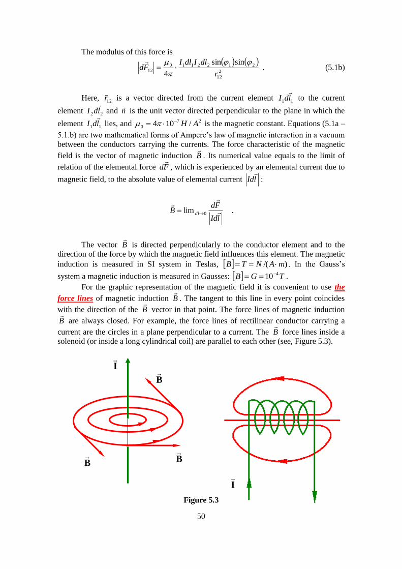
50

The modulus of this force is

2

12

2122110

12

sinsin

4 r

dlIdlIFd

. (5.1b)

Here, 12r is a vector directed from the current element 11 ldI

to the current

element 22 ldI

and n

is the unit vector directed perpendicular to the plane in which the

element 11 ldI

lies, and 27

0 /104 AH is the magnetic constant. Equations (5.1a –

5.1.b) are two mathematical forms of Ampere’s law of magnetic interaction in a vacuum

between the conductors carrying the currents. The force characteristic of the magnetic

field is the vector of magnetic induction B

. Its numerical value equals to the limit of

relation of the elemental force Fd

, which is experienced by an elemental current due to

magnetic field, to the absolute value of elemental current lId

:

lId

FdB dl

0lim .

The vector B

is directed perpendicularly to the conductor element and to the

direction of the force by which the magnetic field influences this element. The magnetic

induction is measured in SI system in Teslas, )/( mANTB . In the Gauss’s

system a magnetic induction is measured in Gausses: TGB 410 . For the graphic representation of the magnetic field it is convenient to use the

force lines of magnetic induction B

. The tangent to this line in every point coincides

with the direction of the B

vector in that point. The force lines of magnetic induction

B

are always closed. For example, the force lines of rectilinear conductor carrying a

current are the circles in a plane perpendicular to a current. The B

force lines inside a

solenoid (or inside a long cylindrical coil) are parallel to each other (see, Figure 5.3).

Figure 5.3

I

B

B

B

I

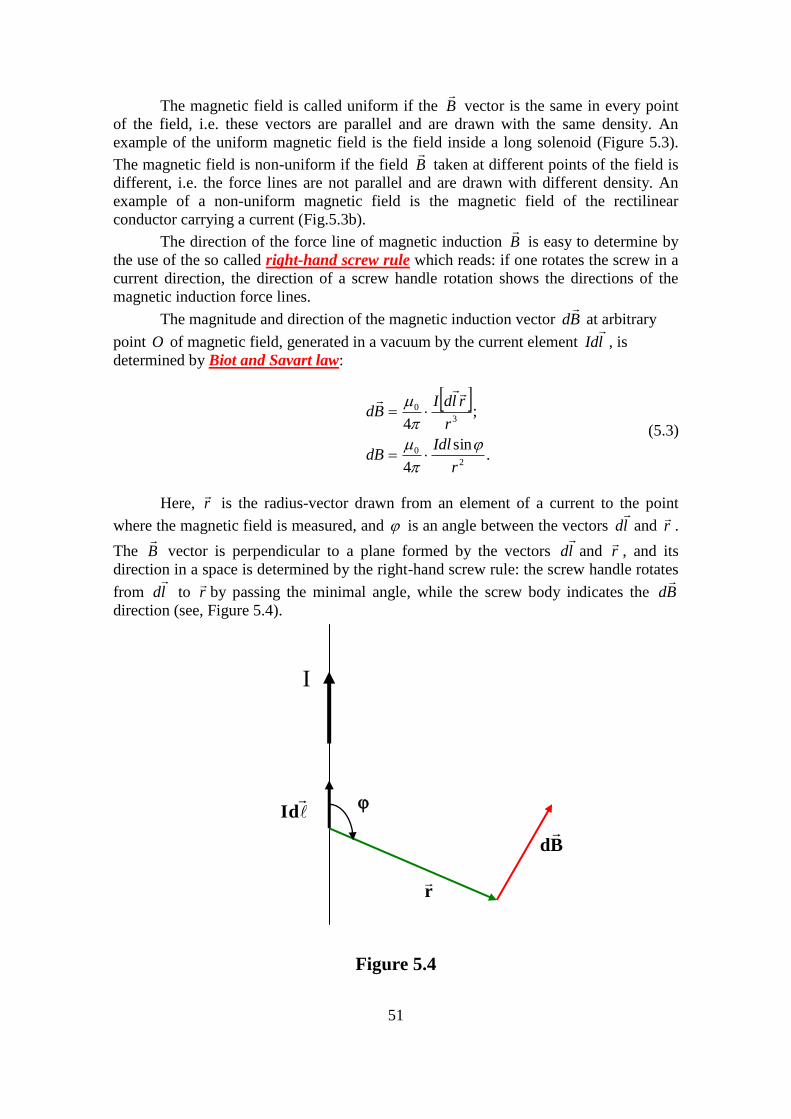
51

The magnetic field is called uniform if the B

vector is the same in every point

of the field, i.e. these vectors are parallel and are drawn with the same density. An

example of the uniform magnetic field is the field inside a long solenoid (Figure 5.3).

The magnetic field is non-uniform if the field B

taken at different points of the field is

different, i.e. the force lines are not parallel and are drawn with different density. An

example of a non-uniform magnetic field is the magnetic field of the rectilinear

conductor carrying a current (Fig.5.3b).

The direction of the force line of magnetic induction B

is easy to determine by

the use of the so called right-hand screw rule which reads: if one rotates the screw in a

current direction, the direction of a screw handle rotation shows the directions of the

magnetic induction force lines.

The magnitude and direction of the magnetic induction vector Bd

at arbitrary

point O of magnetic field, generated in a vacuum by the current element lId

, is

determined by Biot and Savart law:

.sin

4

;4

2

0

3

0

r

IdldB

r

rldIBd

(5.3)

Here, r

is the radius-vector drawn from an element of a current to the point

where the magnetic field is measured, and is an angle between the vectors ld

and r

.

The B

vector is perpendicular to a plane formed by the vectors ld

and r

, and its

direction in a space is determined by the right-hand screw rule: the screw handle rotates

from ld

to r

by passing the minimal angle, while the screw body indicates the Bd

direction (see, Figure 5.4).

Figure 5.4

r

Bd

I

Id

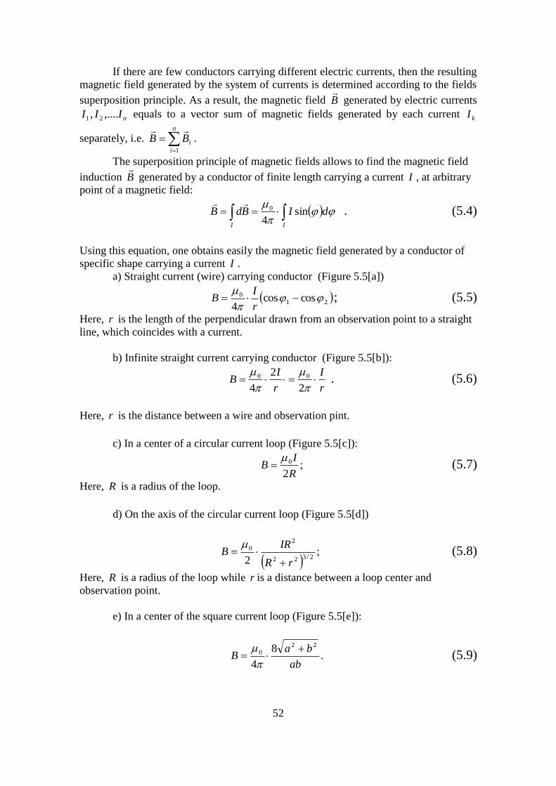
52

If there are few conductors carrying different electric currents, then the resulting

magnetic field generated by the system of currents is determined according to the fields

superposition principle. As a result, the magnetic field B

generated by electric currents

nIII ,...., 21 equals to a vector sum of magnetic fields generated by each current kI

separately, i.e.

n

i

iBB1

.

The superposition principle of magnetic fields allows to find the magnetic field

induction B

generated by a conductor of finite length carrying a current I , at arbitrary

point of a magnetic field:

I I

dIBdB

sin

4

0

. (5.4)

Using this equation, one obtains easily the magnetic field generated by a conductor of

specific shape carrying a current I .

a) Straight current (wire) carrying conductor (Figure 5.5[a])

21

0 coscos4

r

IB ; (5.5)

Here, r is the length of the perpendicular drawn from an observation point to a straight

line, which coincides with a current.

b) Infinite straight current carrying conductor (Figure 5.5[b]):

r

I

r

IB

2

2

4

00 . (5.6)

Here, r is the distance between a wire and observation pint.

c) In a center of a circular current loop (Figure 5.5[c]):

;2

0

R

IB

(5.7)

Here, R is a radius of the loop.

d) On the axis of the circular current loop (Figure 5.5[d])

;

2 2/322

20

rR

IRB

(5.8)

Here, R is a radius of the loop while r is a distance between a loop center and

observation point.

e) In a center of the square current loop (Figure 5.5[e]):

.8

4

22

0

ab

baB

(5.9)

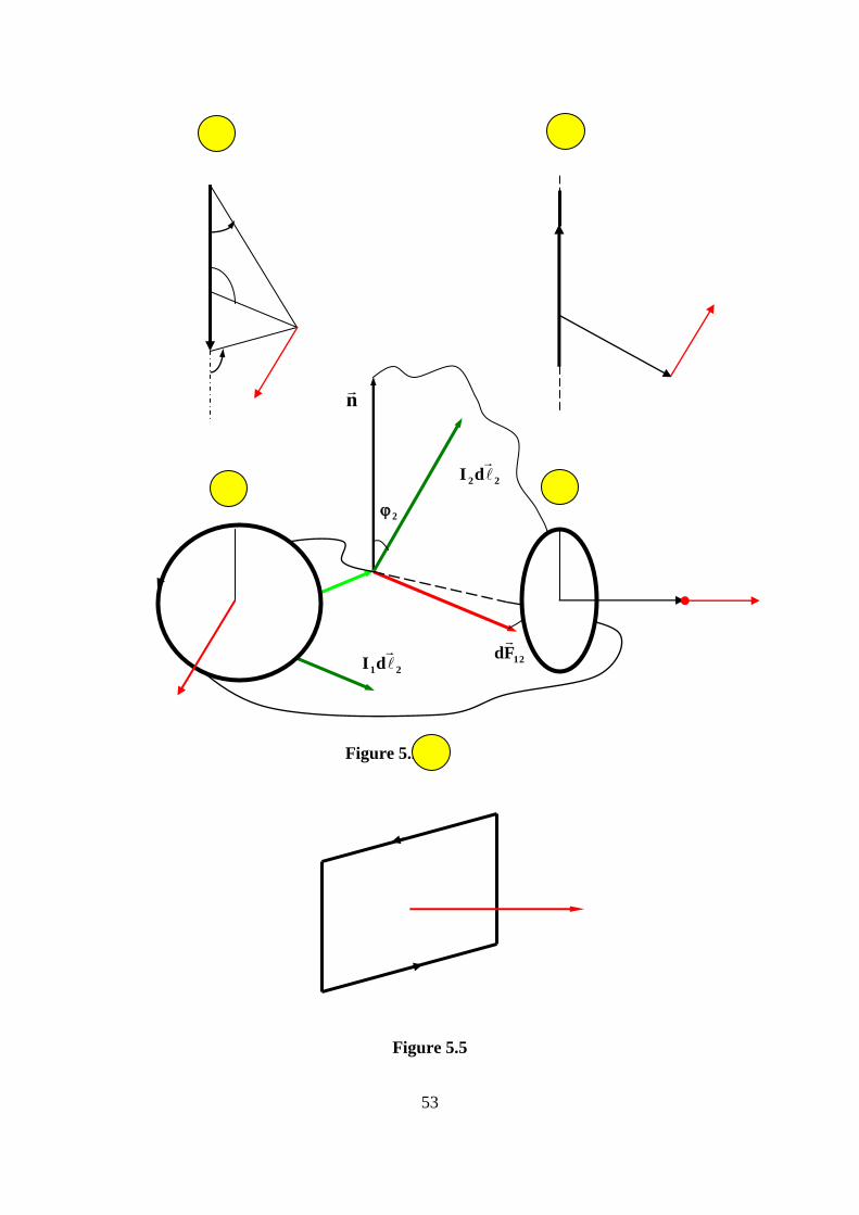
53

Figure 5.5

Figure 5.2

n

2

12Fd

22dI

12r

21dI

1

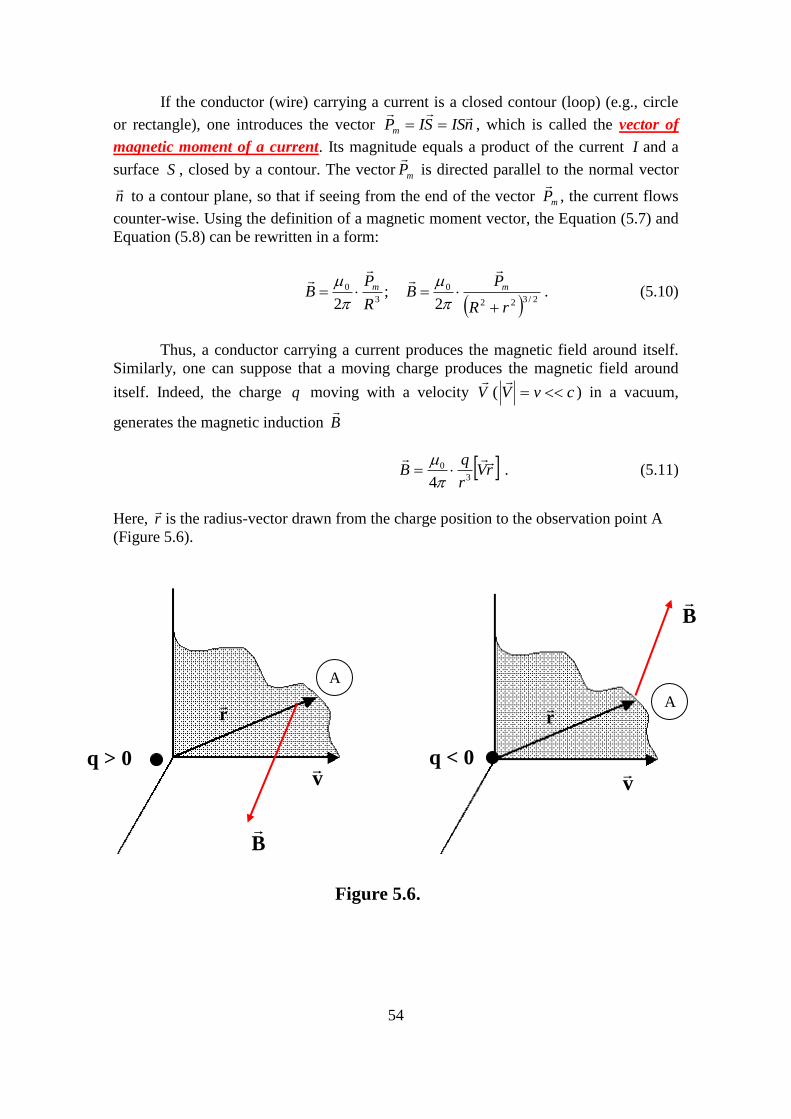
54

If the conductor (wire) carrying a current is a closed contour (loop) (e.g., circle

or rectangle), one introduces the vector nISSIPm

, which is called the vector of

magnetic moment of a current. Its magnitude equals a product of the current I and a

surface S , closed by a contour. The vector mP

is directed parallel to the normal vector

n

to a contour plane, so that if seeing from the end of the vector mP

, the current flows

counter-wise. Using the definition of a magnetic moment vector, the Equation (5.7) and

Equation (5.8) can be rewritten in a form:

;2 3

0

R

PB m

2/322

0

2 rR

PB m

. (5.10)

Thus, a conductor carrying a current produces the magnetic field around itself.

Similarly, one can suppose that a moving charge produces the magnetic field around

itself. Indeed, the charge q moving with a velocity V

( cvV

) in a vacuum,

generates the magnetic induction B

rVr

qB

3

0

4

. (5.11)

Here, r

is the radius-vector drawn from the charge position to the observation point A

(Figure 5.6).

q > 0 v

B

q < 0

v

B

Figure 5.6.

r

r

A

A

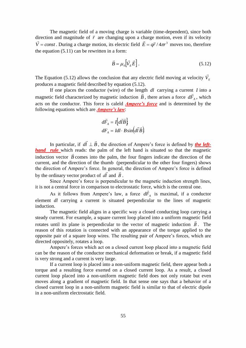
55

The magnetic field of a moving charge is variable (time-dependent), since both

direction and magnitude of r

are changing upon a charge motion, even if its velocity

constV

. During a charge motion, its electric field 34/ rrqE

moves too, therefore

the equation (5.11) can be rewritten in a form:

EVB E

0 . (5.12)

The Equation (5.12) allows the conclusion that any electric field moving at velocity EV

produces a magnetic field described by equation (5.12).

If one places the conductor (wire) of the length dl carrying a current I into a

magnetic field characterized by magnetic induction B

, there arises a force AFd

, which

acts on the conductor. This force is caleld Ampere’s force and is determined by the

following equations which are Ampere’s law:

.sin

;

BldBIdldF

BIdIFd

A

A

In particular, if Bld

, the direction of Ampere’s force is defined by the left-

hand rule which reads: the palm of the left hand is situated so that the magnetic

induction vector B

comes into the palm, the four fingers indicate the direction of the

current, and the direction of the thumb (perpendicular to the other four fingers) shows

the direction of Ampere’s force. In general, the direction of Ampere’s force is defined

by the ordinary vector product of ld

and B

.

Since Ampere’s force is perpendicular to the magnetic induction strength lines,

it is not a central force in comparison to electrostatic force, which is the central one.

As it follows from Ampere’s law, a force AFd

is maximal, if a conductor

element dl carrying a current is situated perpendicular to the lines of magnetic

induction.

The magnetic field aligns in a specific way a closed conducting loop carrying a

steady current. For example, a square current loop placed into a uniform magnetic field

rotates until its plane is perpendicular to the vector of magnetic induction B

. The

reason of this rotation is connected with an appearance of the torque applied to the

opposite pair of a square loop wires. The resulting pair of Ampere’s forces, which are

directed oppositely, rotates a loop.

Ampere’s forces which act on a closed current loop placed into a magnetic field

can be the reason of the conductor mechanical deformation or break, if a magnetic field

is very strong and a current is very large.

If a current loop is placed into a non-uniform magnetic field, there appear both a

torque and a resulting force exerted on a closed current loop. As a result, a closed

current loop placed into a non-uniform magnetic field does not only rotate but even

moves along a gradient of magnetic field. In that sense one says that a behavior of a

closed current loop in a non-uniform magnetic field is similar to that of electric dipole

in a non-uniform electrostatic field.

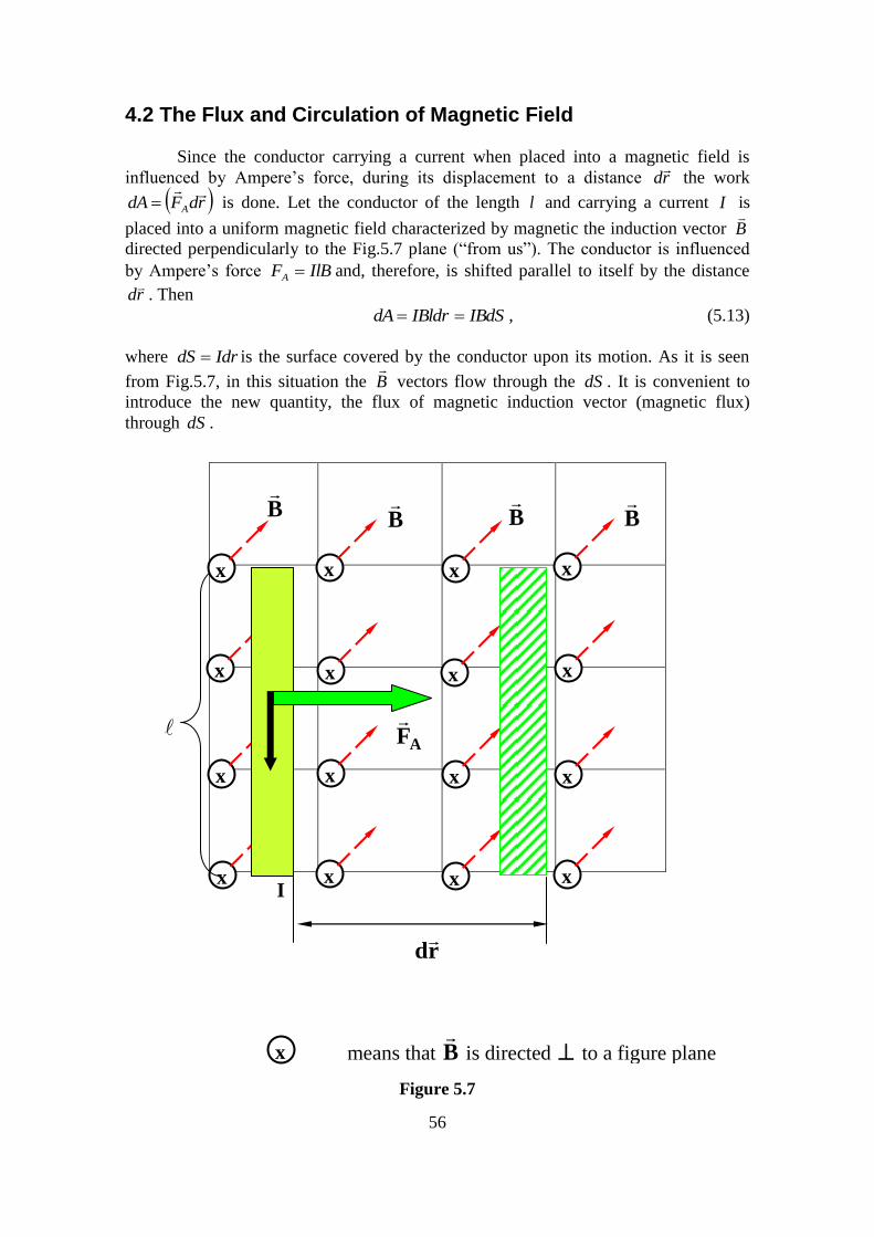
56

4.2 The Flux and Circulation of Magnetic Field

Since the conductor carrying a current when placed into a magnetic field is

influenced by Ampere’s force, during its displacement to a distance rd

the work

rdFdA A

is done. Let the conductor of the length l and carrying a current I is

placed into a uniform magnetic field characterized by magnetic the induction vector B

directed perpendicularly to the Fig.5.7 plane (“from us”). The conductor is influenced

by Ampere’s force IlBFA and, therefore, is shifted parallel to itself by the distance

rd

. Then

IBdSIBldrdA , (5.13)

where IdrdS is the surface covered by the conductor upon its motion. As it is seen

from Fig.5.7, in this situation the B

vectors flow through the dS . It is convenient to

introduce the new quantity, the flux of magnetic induction vector (magnetic flux)

through dS .

Figure 5.7

x

x

x

x x x

x x x x

x x x

x x x

AF

rd

x means that B

is directed to a figure plane

(«from us»)

B

B

B

B

I

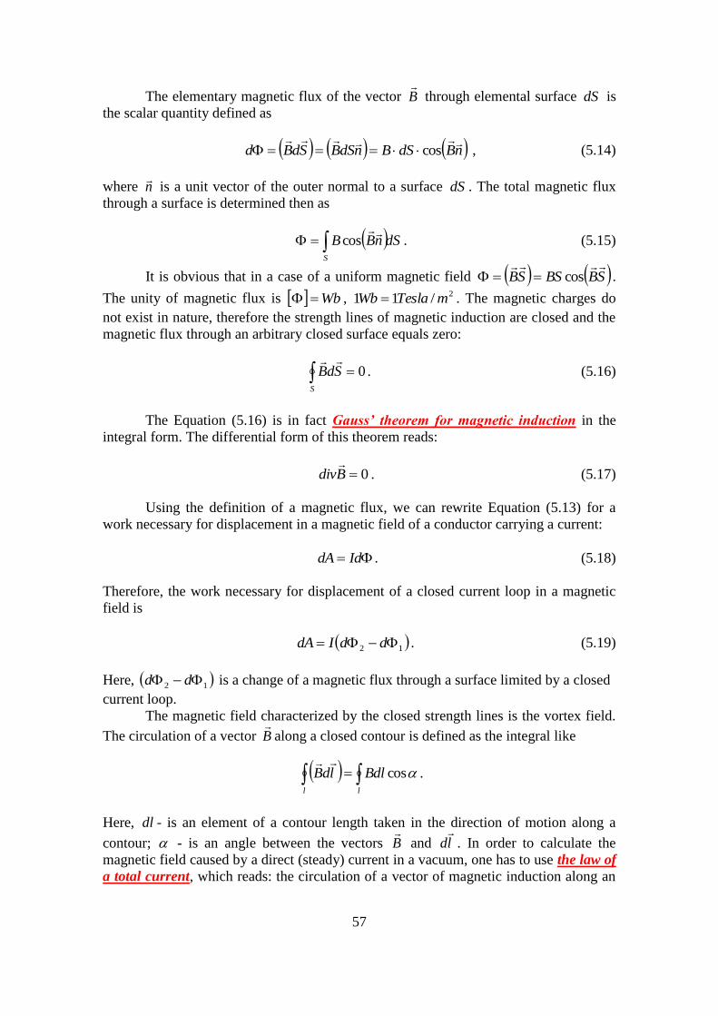
57

The elementary magnetic flux of the vector B

through elemental surface dS is

the scalar quantity defined as

nBdSBndSBSdBd

cos , (5.14)

where n

is a unit vector of the outer normal to a surface dS . The total magnetic flux

through a surface is determined then as

dSnBBS

cos . (5.15)

It is obvious that in a case of a uniform magnetic field SBBSSB

cos .

The unity of magnetic flux is Wb , 2/11 mTeslaWb . The magnetic charges do

not exist in nature, therefore the strength lines of magnetic induction are closed and the

magnetic flux through an arbitrary closed surface equals zero:

S

SdB 0

. (5.16)

The Equation (5.16) is in fact Gauss’ theorem for magnetic induction in the

integral form. The differential form of this theorem reads:

0Bdiv

. (5.17)

Using the definition of a magnetic flux, we can rewrite Equation (5.13) for a

work necessary for displacement in a magnetic field of a conductor carrying a current:

IddA . (5.18)

Therefore, the work necessary for displacement of a closed current loop in a magnetic

field is

12 ddIdA . (5.19)

Here, 12 dd is a change of a magnetic flux through a surface limited by a closed

current loop.

The magnetic field characterized by the closed strength lines is the vortex field.

The circulation of a vector B

along a closed contour is defined as the integral like

ll

BdlldB cos

.

Here, dl - is an element of a contour length taken in the direction of motion along a

contour; - is an angle between the vectors B

and ld

. In order to calculate the

magnetic field caused by a direct (steady) current in a vacuum, one has to use the law of

a total current, which reads: the circulation of a vector of magnetic induction along an

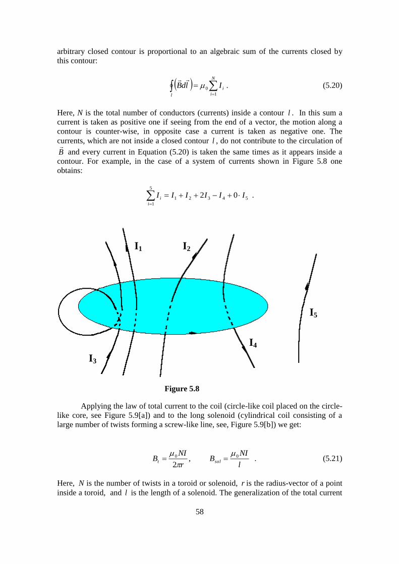
58

arbitrary closed contour is proportional to an algebraic sum of the currents closed by

this contour:

N

i

i

l

IldB1

0

. (5.20)

Here, N is the total number of conductors (currents) inside a contour l . In this sum a

current is taken as positive one if seeing from the end of a vector, the motion along a

contour is counter-wise, in opposite case a current is taken as negative one. The

currents, which are not inside a closed contour l , do not contribute to the circulation of

B

and every current in Equation (5.20) is taken the same times as it appears inside a

contour. For example, in the case of a system of currents shown in Figure 5.8 one

obtains:

5

1

54321 02i

i IIIIII .

Applying the law of total current to the coil (circle-like coil placed on the circle-

like core, see Figure 5.9[a]) and to the long solenoid (cylindrical coil consisting of a

large number of twists forming a screw-like line, see, Figure 5.9[b]) we get:

,2

0

r

NIBt

l

NIBsol

0 . (5.21)

Here, N is the number of twists in a toroid or solenoid, r is the radius-vector of a point

inside a toroid, and l is the length of a solenoid. The generalization of the total current

I1 I2

I3

I4

I5

Figure 5.8

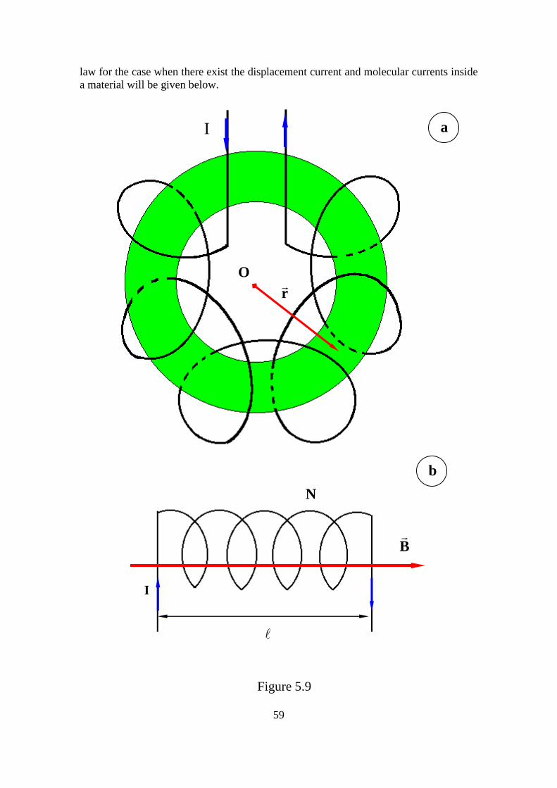
59

law for the case when there exist the displacement current and molecular currents inside

a material will be given below.

b

N

B

Figure 5.9

I

r

O

a

I

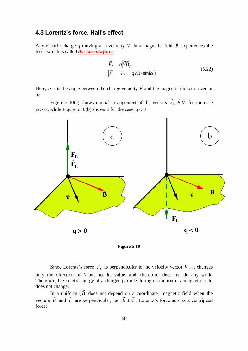
60

4.3 Lorentz’s force. Hall’s effect

Any electric charge q moving at a velocity V

in a magnetic field B

experiences the

force which is called the Lorentz force:

.sin

,

qVBFF

BVqF

LL

L

(5.22)

Here, - is the angle between the charge velocity V

and the magnetic induction vector

B

.

Figure 5.10(a) shows mutual arrangement of the vectors VBFL

,, for the case

0q , while Figure 5.10(b) shows it for the case 0q .

Since Lorentz’s force LF

is perpendicular to the velocity vector V

, it changes

only the direction of V

but not its value, and, therefore, does not do any work.

Therefore, the kinetic energy of a charged particle during its motion in a magnetic field

does not change.

In a uniform ( B

does not depend on a coordinate) magnetic field when the

vectors B

and V

are perpendicular, i.e. VB

, Lorentz’s force acts as a centripetal

force:

LF

LF

v

B

0q 0q

v

B

Figure 5.10

LF

a b

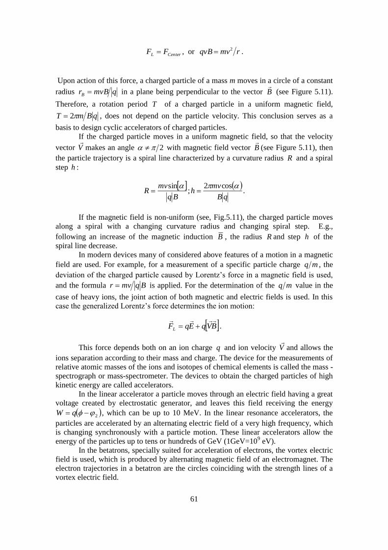
61

CenterL FF , or rmvqvB 2 .

Upon action of this force, a charged particle of a mass m moves in a circle of a constant

radius qmvBrB in a plane being perpendicular to the vector B

(see Figure 5.11).

Therefore, a rotation period T of a charged particle in a uniform magnetic field,

qBmT 2 , does not depend on the particle velocity. This conclusion serves as a

basis to design cyclic accelerators of charged particles.

If the charged particle moves in a uniform magnetic field, so that the velocity

vector V

makes an angle 2 with magnetic field vector B

(see Figure 5.11), then

the particle trajectory is a spiral line characterized by a curvature radius R and a spiral

step h :

.

cos2;

sin

qB

mvh

Bq

mvR

If the magnetic field is non-uniform (see, Fig.5.11), the charged particle moves

along a spiral with a changing curvature radius and changing spiral step. E.g.,

following an increase of the magnetic induction B , the radius R and step h of the

spiral line decrease.

In modern devices many of considered above features of a motion in a magnetic

field are used. For example, for a measurement of a specific particle charge mq , the

deviation of the charged particle caused by Lorentz’s force in a magnetic field is used,

and the formula Bqmvr is applied. For the determination of the mq value in the

case of heavy ions, the joint action of both magnetic and electric fields is used. In this

case the generalized Lorentz’s force determines the ion motion:

BVqEqFL

.

This force depends both on an ion charge q and ion velocity V

and allows the

ions separation according to their mass and charge. The device for the measurements of

relative atomic masses of the ions and isotopes of chemical elements is called the mass -

spectrograph or mass-spectrometer. The devices to obtain the charged particles of high

kinetic energy are called accelerators.

In the linear accelerator a particle moves through an electric field having a great

voltage created by electrostatic generator, and leaves this field receiving the energy

2 qW , which can be up to 10 MeV. In the linear resonance accelerators, the

particles are accelerated by an alternating electric field of a very high frequency, which

is changing synchronously with a particle motion. These linear accelerators allow the

energy of the particles up to tens or hundreds of GeV (1GeV=109 eV).

In the betatrons, specially suited for acceleration of electrons, the vortex electric

field is used, which is produced by alternating magnetic field of an electromagnet. The

electron trajectories in a betatron are the circles coinciding with the strength lines of a

vortex electric field.

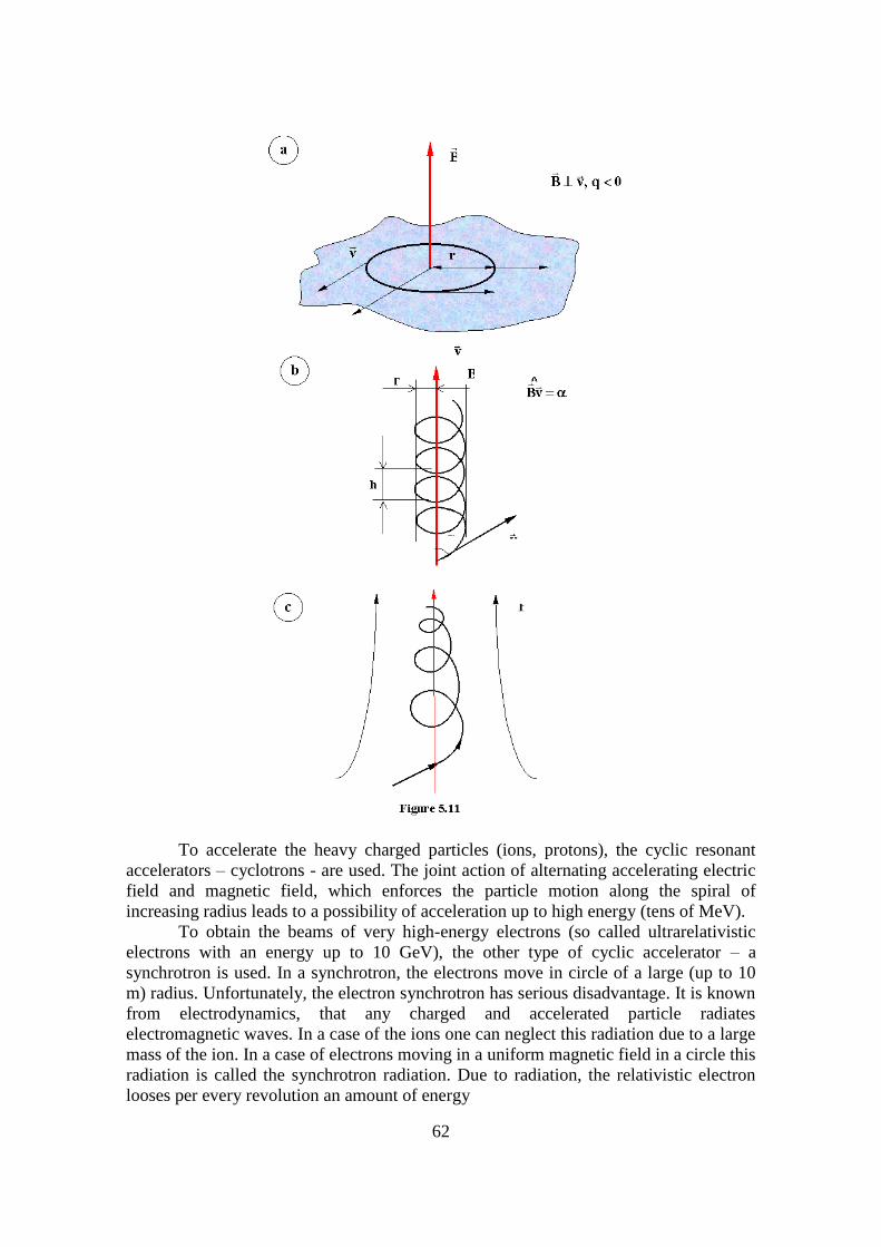
62

To accelerate the heavy charged particles (ions, protons), the cyclic resonant

accelerators – cyclotrons - are used. The joint action of alternating accelerating electric

field and magnetic field, which enforces the particle motion along the spiral of

increasing radius leads to a possibility of acceleration up to high energy (tens of MeV).

To obtain the beams of very high-energy electrons (so called ultrarelativistic

electrons with an energy up to 10 GeV), the other type of cyclic accelerator – a

synchrotron is used. In a synchrotron, the electrons move in circle of a large (up to 10

m) radius. Unfortunately, the electron synchrotron has serious disadvantage. It is known

from electrodynamics, that any charged and accelerated particle radiates

electromagnetic waves. In a case of the ions one can neglect this radiation due to a large

mass of the ion. In a case of electrons moving in a uniform magnetic field in a circle this

radiation is called the synchrotron radiation. Due to radiation, the relativistic electron

looses per every revolution an amount of energy

63

R

EconstWrad

4

.

Here, RE, are the energy of relativistic electron and an orbit radius, respectively.

Therefore, this radiation energy loss must be compensated by additional acceleration in

order to keep the electron energy constant. The advantage is that the synchrotron

radiation is widely used through the world as the bright source of soft X-rays, which are

used in lithography and in biological and medical research.

In electronic optics one studies the properties of charged particle beams

(electrons, protons) interacting with electric and magnetic fields. In particular, the

diffraction phenomena are studied, which are connected with the wave properties of the

particles.

Hall’s effect is called a phenomenon when the voltage and transverse

electric field arises in a metal or semiconductor carrying an electric current I , if they

are placed into a magnetic field, which is perpendicular to the current direction. Let the

metal conductor be placed into magnetic field characterized by the magnetic induction

B

, as shown in Figure 5.12.

Under the action of Lorentz’s force LF , the conductivity electrons are deflected

to the upper surface of the conductor. Therefore, the enhanced concentration of positive

charges arises near the lower surface. These two oppositely charged surfaces causes the

transverse electric field E

. When it reaches a definite value, the stationary distribution

of charges is established and the voltage can be found using the equation

h

IBR , (5.24)

with qnR 1 being Hall’s constant ( nq, are the charge of particle causing the current

and their concentration, respectively). The vector E

is defined by the equation

Figure 5.12

q v

h

q<0

B

B

+ + + +

- - - -

I E

LF

64

jBRE

,

Here, j

- is the vector of the current density. Hall’s effect allows to determine the

concentration of the current carriers and to make conclusions on the type of

conductivity (e.g., in the case of semiconductors to conclude on hole, electronic or

mixed – n and p type - conductance).

Indeed, the sign of Hall’s constant coincides with a sign of the charge of the

particles, which are responsible for a conductance of a material. Therefore, if one

measures Hall’s constant R for a semiconductor, one can say that a conductance is

electronic one if R<0 and is hole-type if R<0.

From the other side, if Hall’s constant and charge of current carriers and their

nature are known one can determine their concentration. E.g., for metals

qnn 1 ,

which coincides with atomic concentration.

In a case of electronic conductance, one can use the R value to estimate the mean

free path of electrons in a conductor. Indeed, the specific electric conductance is

defined as

um

ne

2

2 .

Here, m, and u are the mass of electron, its mean free path and mean velocity of

thermal motion, respectively. Therefore, the mean free path of electrons is defined by

following equation:

e

Rum

ne

um

222

.

An estimation according this formula reads that the mean free path of electrons in a

conductor is hundreds of interatomic distances, i.e. m810 .

65

4.4 Electromagnetic induction

The phenomenon of electromagnetic induction discovered by the great English

physicist M.Faraday (1831) is the appearance of electric induction i in a conducting

contour placed into an alternating magnetic field. If the contour is closed, there appears

an inductive electric current inside it. The law of electromagnetic induction ( Faraday’s

law) reads: the electric induction in a contour is equal and has an opposite sign to the

rapidity of a change of magnetic flux through the surface closed by this contour:

dt

di

. (5.25)

The direction of the path along a contour is selected in the following way: if

seeing from the end of a normal external vector n

to the contour surface, this path is

counter-clockwise. If a closed contour consists of N connected coils, then is the

total magnetic flux through the surfaces limited by all N coils, namely

N

i

i

1

,

Here, - is the contour coupling flux. Therefore,

dt

di

.

The minus sign in Equation (5.25) is determined by Lentz’s rule: an induction

current I in a contour has always the same direction as the magnetic field created by it,

and the magnetic flux through the surface limited by a contour prevents the change of

magnetic flux, which causes this induction current.

The magnetic flux in Equation (5.25) can be different due to a change of the

contour size (e.g., its deformation), or due to the movement of the contour (e.g.,

rotation) in an external magnetic field, or due to a change of the magnetic field in time.

For example, under rotation of a frame in uniform magnetic field constB at a

constant angular velocity , the magnetic flux is tBS cos , and therefore there

appears an alternating electric induction tBSi sin . This effect is used in the

alternating current generators.

The induction currents, which appear in the bulk of the conductors are named

the vortex currents or Foucault’s currents. Foucault’s currents obey Lentz’s law: their

magnetic field is directed in the way in order to prevent a change of the magnetic flux

which induces the vortex currents. These currents cause the heating of the conductors:

the amount of the heat generated by vortex currents per time unit is directly proportional

to the frequency squared of the magnetic flux change.

The appearance of an electric induction in a circuit during a change of a current

in this circuit is named the self-induction. The self magnetic field of a current in a

contour creates the magnetic flux through the surface S closed by the contour. One

says that the magnetic flux is coupled with a contour,

66

LI . (5.26)

Here, L - is the inductivity of a contour. The inductivity L is measured in Henrey:

1Hn=Vsec/A. The inductivity L depends on the geometric form of a contour, its size,

and on the properties of a media where this contour is placed. For example, the

inductivity of a solenoid of a length l and a surface of cross-section S and the number

of twists N is:

l

SNL

2

0 . (5.27)

By substituting of Equation (5.26) into Equation (5.25) one obtains:

dt

dILi . (5.28)

That means, the contour inductivity is a measure of its inertia with respect to the

current change.

If there are two contours 1 and 2 near each other, and the current strength

changes in one of them, in the second one appears an electromagnetic induction. The

law of mutual induction is written in the form:

dt

dIL

dt

dIL 2

1211

212 ; . (5.29)

The coefficients constLL 2112 are named the coefficients of mutual

inductivity of contours 1 and 2. In particular, the principle of the work of transformers,

which are used to increase or decrease the voltage of alternating current, is based on the

phenomenon of mutual induction: the alternating magnetic field of the current I in the

primary winding causes an appearance of mutual electric induction in the secondary

winding. The core provides a sufficient mutual inductivity 12L of the transformer.

The magnetic field of an electric current has an energy which can be expressed

as:

2

2

1LIWm . (5.30)

For example, the energy of magnetic field of a long solenoid in a vacuum is:

VInWm

22

02

1 , (5.31)

Here, V - is the volume of a solenoid, n - is the number of the twists per its

length unit. In order to obtain the amount of energy closed in a unit volume of a field,

one introduces the definition of the volume density of the energy m :

67

BHHB

dV

dWm

2

1

2

1

2

1 2

0

0

2

, (5.32)

Here, 0BH is named the strength of a magnetic field in a vacuum.

Problems to Chapter 4 (Magnetic field)

Problem 1 Calculate the magnitude of the magnetic field at a distance 100 cm from a long, thin

conductor carrying a current of 1.0 A.

Problem 2 A long, thin conductor carries a current of 10.0 A. At what distance from the conductor

the magnitude of the resulting magnetic field equals 1.0010-4

T ?

Problem 3 A wire in which there is a current of 5.0 A is to be formed into a circular loop of one

turn. If the required value of the magnetic field at the center of the loop is 10.0 T, what

is the required radius of the loop?

Problem 4 In Bohr's model of the hydrogen atom (1913), an electron circles the proton at a

distance of 5.310-11

m with a speed of 2.2106 m/s. Compute the magnetic field strength

which produces this motion at the location of the proton.

Problem 5

A 12-cm 16-cm rectangular loop of superconducting wire carries a current of 30 A.

What is the magnetic field at the center of the loop?

Problem 6 A long, straight wire lies on a horizontal table and carries a current of 1.2 A. A proton

moves parallel to the wire (opposite the current) with a constant speed of 2.3104 m/s at

a distance d above the wire. Determine the value of d. You may ignore the magnetic

field due to the Earth.

Problem 7 The magnetic coil of a tokamak fusion reactor is in the shape of a toroid having an inner

radius of 0.70 m and outer radius of 1.30 m. If the toroid has 900 turns of large-diameter

wire, each of which carries a current of 14 kA, find the magnetic field strength along (a)

the inner radius and (b) the outer radius.

Problem 8 A packed bundle of 100 long straight, insulated wires forms a cylinder of radius

R = 0.5 cm. (a) If each wire carries a current of 2.0 A, what are the magnitude and

direction of the magnetic force per unit length acting on a wire located 0.2 cm from the

center of the bundle? (b) Would a wire on the outer edge of the bundle experience a

force greater or smaller than the value calculated in part (a)?

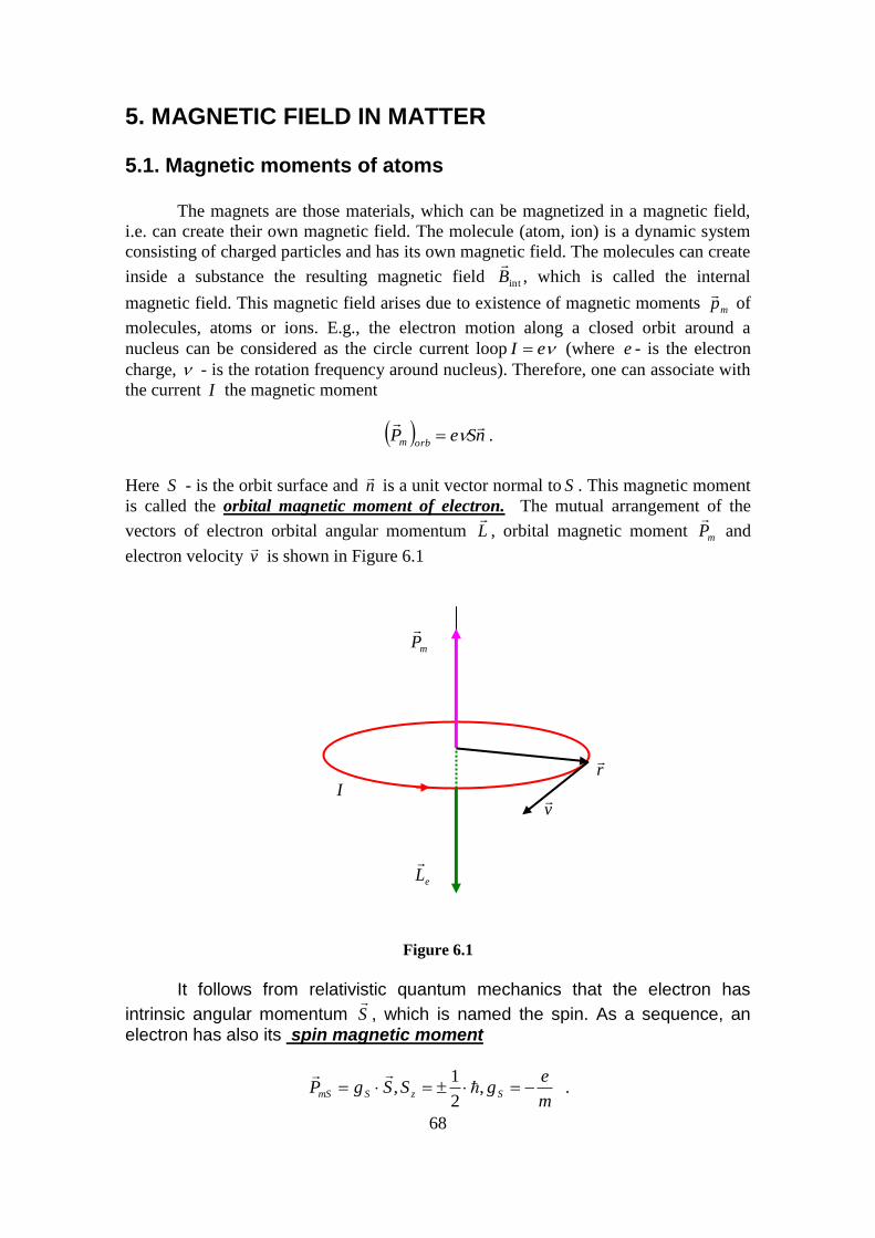
68

5. MAGNETIC FIELD IN MATTER

5.1. Magnetic moments of atoms

The magnets are those materials, which can be magnetized in a magnetic field,

i.e. can create their own magnetic field. The molecule (atom, ion) is a dynamic system

consisting of charged particles and has its own magnetic field. The molecules can create

inside a substance the resulting magnetic field intB

, which is called the internal

magnetic field. This magnetic field arises due to existence of magnetic moments mp

of

molecules, atoms or ions. E.g., the electron motion along a closed orbit around a

nucleus can be considered as the circle current loop eI (where e - is the electron

charge, - is the rotation frequency around nucleus). Therefore, one can associate with

the current I the magnetic moment

nSePorbm

.

Here S - is the orbit surface and n

is a unit vector normal to S . This magnetic moment

is called the orbital magnetic moment of electron. The mutual arrangement of the

vectors of electron orbital angular momentum L

, orbital magnetic moment mP

and

electron velocity v

is shown in Figure 6.1

mP

r

I v

eL

Figure 6.1

It follows from relativistic quantum mechanics that the electron has

intrinsic angular momentum S

, which is named the spin. As a sequence, an electron has also its spin magnetic moment

m

egSSgP SzSmS ,

2

1,

.

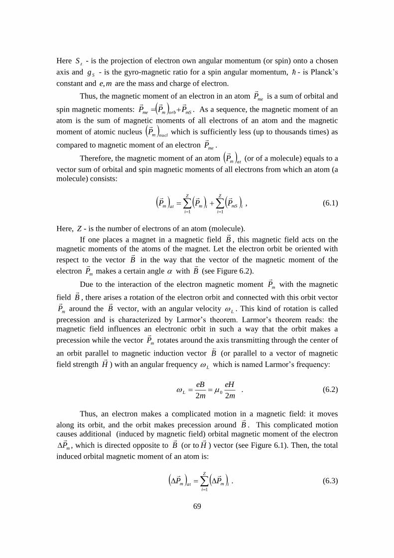
69

Here zS - is the projection of electron own angular momentum (or spin) onto a chosen

axis and Sg - is the gyro-magnetic ratio for a spin angular momentum, - is Planck’s

constant and me, are the mass and charge of electron.

Thus, the magnetic moment of an electron in an atom meP

is a sum of orbital and

spin magnetic moments: mSorbmme PPP

. As a sequence, the magnetic moment of an

atom is the sum of magnetic moments of all electrons of an atom and the magnetic

moment of atomic nucleus nuclmP

which is sufficiently less (up to thousands times) as

compared to magnetic moment of an electron meP

.

Therefore, the magnetic moment of an atom atmP

(or of a molecule) equals to a

vector sum of orbital and spin magnetic moments of all electrons from which an atom (a

molecule) consists:

Z

iimS

Z

iimatm PPP

11

, (6.1)

Here, Z - is the number of electrons of an atom (molecule).

If one places a magnet in a magnetic field B

, this magnetic field acts on the

magnetic moments of the atoms of the magnet. Let the electron orbit be oriented with

respect to the vector B

in the way that the vector of the magnetic moment of the

electron mP

makes a certain angle with B

(see Figure 6.2).

Due to the interaction of the electron magnetic moment mP

with the magnetic

field B

, there arises a rotation of the electron orbit and connected with this orbit vector

mP

around the B

vector, with an angular velocity L . This kind of rotation is called

precession and is characterized by Larmor’s theorem. Larmor’s theorem reads: the

magnetic field influences an electronic orbit in such a way that the orbit makes a

precession while the vector mP

rotates around the axis transmitting through the center of

an orbit parallel to magnetic induction vector B

(or parallel to a vector of magnetic

field strength H

) with an angular frequency L which is named Larmor’s frequency:

m

eH

m

eBL

220 . (6.2)

Thus, an electron makes a complicated motion in a magnetic field: it moves

along its orbit, and the orbit makes precession around B

. This complicated motion

causes additional (induced by magnetic field) orbital magnetic moment of the electron

mP

, which is directed opposite to B

(or to H

) vector (see Figure 6.1). Then, the total

induced orbital magnetic moment of an atom is:

Z

iimatm PP

1

. (6.3)

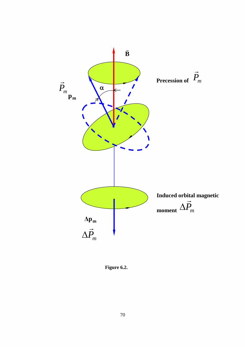
70

mP

mP

Figure 6.2.

B

mp

Induced orbital magnetic

moment mP

Precession of mP

mΔp

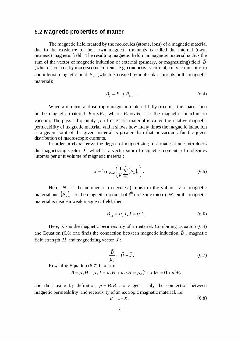
71

5.2 Magnetic properties of matter

The magnetic field created by the molecules (atoms, ions) of a magnetic material

due to the existence of their own magnetic moments is called the internal (own,

intrinsic) magnetic field. The resulting magnetic field in a magnetic material is thus the

sum of the vector of magnetic induction of external (primary, or magnetizing) field B

(which is created by macroscopic currents, e.g. conductivity current, convection current)

and internal magnetic field intB

(which is created by molecular currents in the magnetic

material):

int0 BBB

. (6.4)

When a uniform and isotropic magnetic material fully occupies the space, then

in the magnetic material 0BB

, where HB

0 - is the magnetic induction in

vacuum. The physical quantity of magnetic material is called the relative magnetic

permeability of magnetic material, and it shows how many times the magnetic induction

at a given point of the given material is greater than that in vacuum, for the given

distribution of macroscopic currents.

In order to characterize the degree of magnetizing of a material one introduces

the magnetizing vector J

, which is a vector sum of magnetic moments of molecules

(atoms) per unit volume of magnetic material:

N

iimV P

VJ

1

0

1lim

. (6.5)

Here, N - is the number of molecules (atoms) in the volume V of magnetic

material and imP

- is the magnetic moment of i

th molecule (atom). When the magnetic

material is inside a weak magnetic field, then

HJJB

,0int . (6.6)

Here, - is the magnetic permeability of a material. Combining Equation (6.4)

and Equation (6.6) one finds the connection between magnetic induction B

, magnetic

field strength H

and magnetizing vector J

:

JHB

0

. (6.7)

Rewriting Equation (6.7) in a form

000000 11 BHHHJHB

,

and then using by definition 0BB , one gets easily the connection between

magnetic permeability and receptivity of an isotropic magnetic material, i.e.

1 . (6.8)

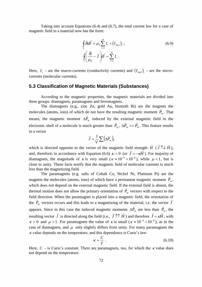
72

Taking into account Equations (6.4) and (6.7), the total current law for a case of

magnetic field in a material now has the form:

l

N

iimoli IIldB

1

0

; (6.9)

l

N

i

iIldJB

10

.

Here, iI - are the macro-currents (conductivity currents) and imolI - are the micro-

currents (molecular currents).

5.3 Classification of Magnetic Materials (Substances)

According to the magnetic properties, the magnetic materials are divided into

three groups: diamagnets, paramagnets and ferromagnets.

The diamagnets (e.g., zinc Zn, gold Au, bismuth Bi) are the magnets the

molecules (atoms, ions) of which do not have the resulting magnetic moment mP

. That

means, the magnetic moment mP

induced by the external magnetic field in the

electronic shell of a molecule is much greater than mP

, mm PP

. This feature results

in a vector

mPV

J 1

,

which is directed opposite to the vector of the magnetic field strength H

( HJ

),

and, therefore, in accordance with Equation (6.6) 0 (or HJ

). For majority of

diamagnets, the magnitude of is very small ( 64 1010 ), while 1 , but is

close to unity. These facts testify that the magnetic field of molecular currents is much

less than the magnetizing field.

The paramagnets (e.g. salts of Cobalt Co, Nickel Ni, Platinum Pt) are the

magnets the molecules (atoms, ions) of which have a permanent magnetic moment mP

,

which does not depend on the external magnetic field. If the external field is absent, the

thermal motion does not allow the primary orientation of mP

vectors with respect to the

field direction. When the paramagnet is placed into a magnetic field, the orientation of

the mP

vectors occurs and this leads to a magnetizing of the material, i.e. the vector J

appears. Since in this case the induced magnetic moments mP

are less than mP

, the

resulting vector J

is directed along the field (i.e., HJ

) and therefore HJ

, with

0 and 1 . For paramagnets the value of is small ( 64 1010 ), as in the

case of diamagnets, and only slightly differs from unity. For many paramagnets the

value depends on the temperature, and this dependence is Curie’s law:

T

C . (6.10)

Here, C - is Curie’s constant. There are paramagnets, too, for which the value does

not depend on the temperature.

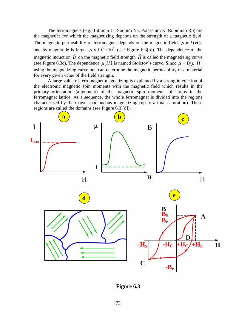
73

The ferromagnets (e.g., Lithium Li, Sodium Na, Potassium K, Rubidium Rb) are

the magnetics for which the magnetizing depends on the strength of a magnetic field.

The magnetic permeability of ferromagnet depends on the magnetic field, )(Hf

,

and its magnitude is large, 53 1010 (see Figure 6.3[b]). The dependence of the

magnetic induction B

on the magnetic field strength H

is called the magnetizing curve

(see Figure 6.3c). The dependence H is named Stoletov’s curve. Since HB 0 ,

using the magnetizing curve one can determine the magnetic permeability of a material

for every given value of the field strength.

A large value of ferromagnet magnetizing is explained by a strong interaction of

the electronic magnetic spin moments with the magnetic field which results in the

primary orientation (alignment) of the magnetic spin moments of atoms in the

ferromagnet lattice. As a sequence, the whole ferromagnet is divided into the regions

characterized by their own spontaneous magnetizing (up to a total saturation). These

regions are called the domains (see Figure 6.3 [d]).

e

B BS

Br

-HC +HC +HS

-Br

A

C

D

H

I

H

Imax

H

1

B

H

а b с

d

-HS

Figure 6.3

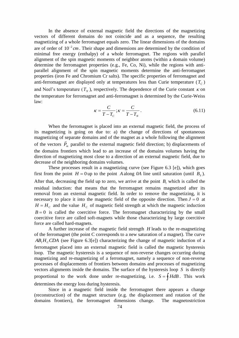
74

In the absence of external magnetic field the directions of the magnetizing

vectors of different domains do not coincide and as a sequence, the resulting

magnetizing of a whole ferromagnet equals zero. The linear dimensions of the domains

are of order of cm210 . Their shape and dimensions are determined by the condition of

minimal free energy (enthalpy) of a whole ferromagnet. The regions with parallel

alignment of the spin magnetic moments of neighbor atoms (within a domain volume)

determine the ferromagnet properties (e.g., Fe, Co, Ni), while the regions with anti-

parallel alignment of the spin magnetic moments determine the anti-ferromagnet

properties (iron Fe and Chromium Cr salts). The specific properties of ferromagnet and

anti-ferromagnet are displayed only at temperatures less than Curie temperature ( CT )

and Neel’s temperature ( NT ), respectively. The dependence of the Curie constant on

the temperature for ferromagnet and anti-ferromagnet is determined by the Curie-Weiss

law:

NC TT

C

TT

C

; . (6.11)

When the ferromagnet is placed into an external magnetic field, the process of

its magnetizing is going on due to: a) the change of directions of spontaneous

magnetizing of separate domains and of the magnet as a whole following the alignment

of the vectors mP

parallel to the external magnetic field direction; b) displacements of

the domains frontiers which lead to an increase of the domains volumes having the

direction of magnetizing most close to a direction of an external magnetic field, due to

decrease of the neighboring domains volumes.

These processes result in a magnetizing curve (see Figure 6.3 [e]), which goes

first from the point 0H up to the point A along 0A line until saturation (until SB ).

After that, decreasing the field up to zero, we arrive at the point lB which is called the

residual induction: that means that the ferromagnet remains magnetized after its

removal from an external magnetic field. In order to remove the magnetizing, it is

necessary to place it into the magnetic field of the opposite direction. Then 0J at

CHH and the value CH of magnetic field strength at which the magnetic induction

0B is called the coercitive force. The ferromagnet characterizing by the small

coercitive force are called soft-magnets while those characterizing by large coercitive

force are called hard-magnets.

A further increase of the magnetic field strength H leads to the re-magnetizing

of the ferromagnet (the point C corresponds to a new saturation of a magnet). The curve

CDAHAB Cl (see Figure 6.3[e]) characterizing the change of magnetic induction of a

ferromagnet placed into an external magnetic field is called the magnetic hysteresis

loop. The magnetic hysteresis is a sequence of non-reverse changes occurring during

magnetizing and re-magnetizing of a ferromagnet, namely a sequence of non-reverse

processes of displacements of frontiers between domains and processes of magnetizing

vectors alignments inside the domains. The surface of the hysteresis loop S is directly

proportional to the work done under re-magnetizing, i.e. HdBS . This work

determines the energy loss during hysteresis.

Since in a magnetic field inside the ferromagnet there appears a change

(reconstruction) of the magnet structure (e.g. the displacement and rotation of the

domains frontiers), the ferromagnet dimensions change. The magnetostriction

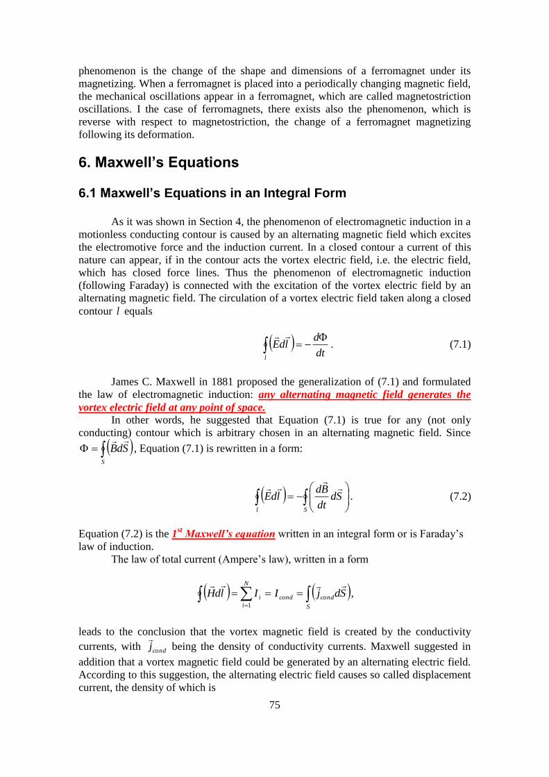
75

phenomenon is the change of the shape and dimensions of a ferromagnet under its

magnetizing. When a ferromagnet is placed into a periodically changing magnetic field,

the mechanical oscillations appear in a ferromagnet, which are called magnetostriction

oscillations. I the case of ferromagnets, there exists also the phenomenon, which is

reverse with respect to magnetostriction, the change of a ferromagnet magnetizing

following its deformation.

6. Maxwell’s Equations

6.1 Maxwell’s Equations in an Integral Form

As it was shown in Section 4, the phenomenon of electromagnetic induction in a

motionless conducting contour is caused by an alternating magnetic field which excites

the electromotive force and the induction current. In a closed contour a current of this

nature can appear, if in the contour acts the vortex electric field, i.e. the electric field,

which has closed force lines. Thus the phenomenon of electromagnetic induction

(following Faraday) is connected with the excitation of the vortex electric field by an

alternating magnetic field. The circulation of a vortex electric field taken along a closed

contour l equals

l

dt

dldE

. (7.1)

James C. Maxwell in 1881 proposed the generalization of (7.1) and formulated

the law of electromagnetic induction: any alternating magnetic field generates the

vortex electric field at any point of space.

In other words, he suggested that Equation (7.1) is true for any (not only

conducting) contour which is arbitrary chosen in an alternating magnetic field. Since

S

SdB

, Equation (7.1) is rewritten in a form:

l S

Sddt

BdldE

. (7.2)

Equation (7.2) is the 1st Maxwell’s equation written in an integral form or is Faraday’s

law of induction.

The law of total current (Ampere’s law), written in a form

N

i S

condcondi SdjIIldH1

,

leads to the conclusion that the vortex magnetic field is created by the conductivity

currents, with condj

being the density of conductivity currents. Maxwell suggested in

addition that a vortex magnetic field could be generated by an alternating electric field.

According to this suggestion, the alternating electric field causes so called displacement

current, the density of which is

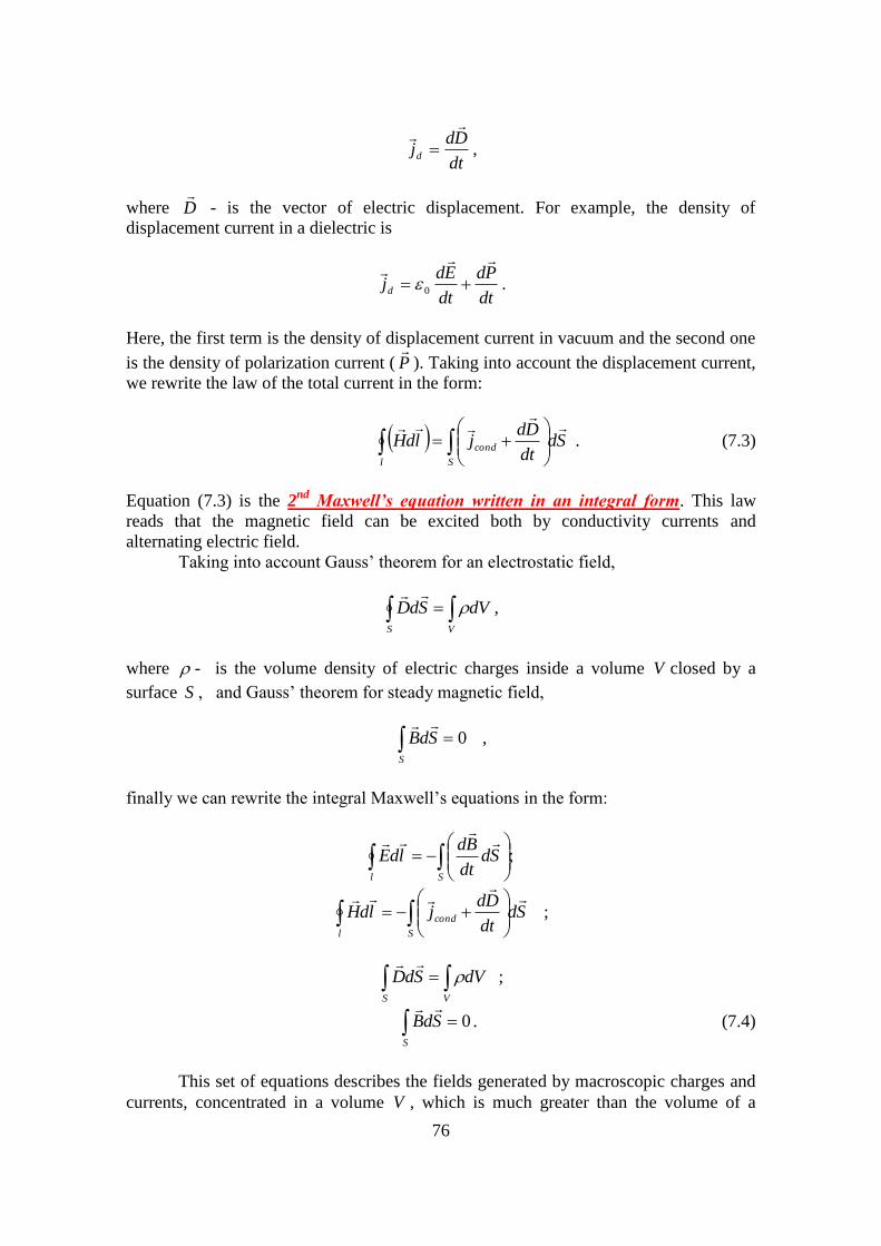
76

dt

Ddjd

,

where D

- is the vector of electric displacement. For example, the density of

displacement current in a dielectric is

dt

Pd

dt

Edjd

0 .

Here, the first term is the density of displacement current in vacuum and the second one

is the density of polarization current ( P

). Taking into account the displacement current,

we rewrite the law of the total current in the form:

Sddt

DdjldH

l S

cond

. (7.3)

Equation (7.3) is the 2nd

Maxwell’s equation written in an integral form. This law

reads that the magnetic field can be excited both by conductivity currents and

alternating electric field.

Taking into account Gauss’ theorem for an electrostatic field,

S V

dVSdD

,

where - is the volume density of electric charges inside a volume V closed by a

surface S , and Gauss’ theorem for steady magnetic field,

S

SdB 0

,

finally we can rewrite the integral Maxwell’s equations in the form:

;

l S

Sddt

BdldE

Sddt

DdjldH

l S

cond

;

S V

dVSdD

;

S

SdB 0

. (7.4)

This set of equations describes the fields generated by macroscopic charges and

currents, concentrated in a volume V , which is much greater than the volume of a

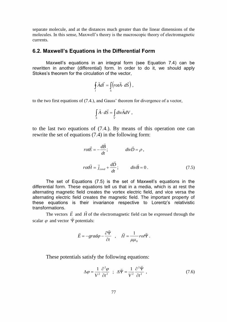
77

separate molecule, and at the distances much greater than the linear dimensions of the

molecules. In this sense, Maxwell’s theory is the macroscopic theory of electromagnetic

currents.

6.2. Maxwell’s Equations in the Differential Form

Maxwell’s equations in an integral form (see Equation 7.4) can be rewritten in another (differential) form. In order to do it, we should apply Stokes’s theorem for the circulation of the vector,

l S

SdArotldA

,

to the two first equations of (7.4.), and Gauss’ theorem for divergence of a vector,

VS

dVAdivSdA

,

to the last two equations of (7.4.). By means of this operation one can

rewrite the set of equations (7.4) in the following form:

;dt

BdErot

Ddiv

,

dt

DdjHrot cond

; 0Bdiv

. (7.5)

The set of Equations (7.5) is the set of Maxwell’s equations in the differential form. These equations tell us that in a media, which is at rest the alternating magnetic field creates the vortex electric field, and vice versa the alternating electric field creates the magnetic field. The important property of these equations is their invariance respective to Lorentz’s relativistic transformations.

The vectors E

and H

of the electromagnetic field can be expressed through the

scalar and vector

potentials:

tgradE

,

rotH0

1

.

These potentials satisfy the following equations:

2

2

2

1

tV

;

2

2

2

1

tV

, (7.6)

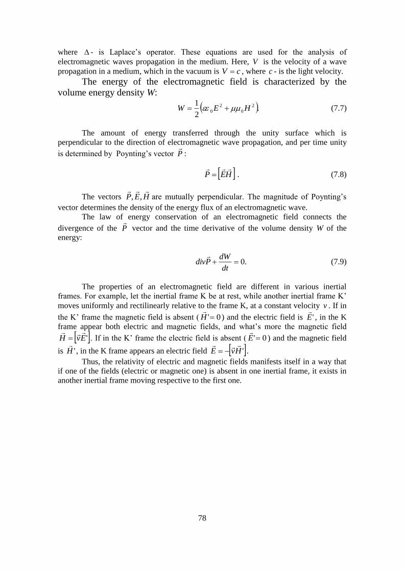
78

where - is Laplace’s operator. These equations are used for the analysis of

electromagnetic waves propagation in the medium. Here, V is the velocity of a wave

propagation in a medium, which in the vacuum is cV , where c - is the light velocity.

The energy of the electromagnetic field is characterized by the

volume energy density W:

.2

1 2

0

2

0 HEW (7.7)

The amount of energy transferred through the unity surface which is

perpendicular to the direction of electromagnetic wave propagation, and per time unity

is determined by Poynting’s vector P

:

HEP

. (7.8)

The vectors HEP

,, are mutually perpendicular. The magnitude of Poynting’s

vector determines the density of the energy flux of an electromagnetic wave.

The law of energy conservation of an electromagnetic field connects the

divergence of the P

vector and the time derivative of the volume density W of the

energy:

.0dt

dWPdiv

(7.9)

The properties of an electromagnetic field are different in various inertial

frames. For example, let the inertial frame K be at rest, while another inertial frame K’

moves uniformly and rectilinearly relative to the frame K, at a constant velocity v . If in

the K’ frame the magnetic field is absent ( 0'H

) and the electric field is 'E

, in the K

frame appear both electric and magnetic fields, and what’s more the magnetic field

'EvH

. If in the K’ frame the electric field is absent ( 0'E

) and the magnetic field

is 'H

, in the K frame appears an electric field 'HvE

.

Thus, the relativity of electric and magnetic fields manifests itself in a way that

if one of the fields (electric or magnetic one) is absent in one inertial frame, it exists in

another inertial frame moving respective to the first one.

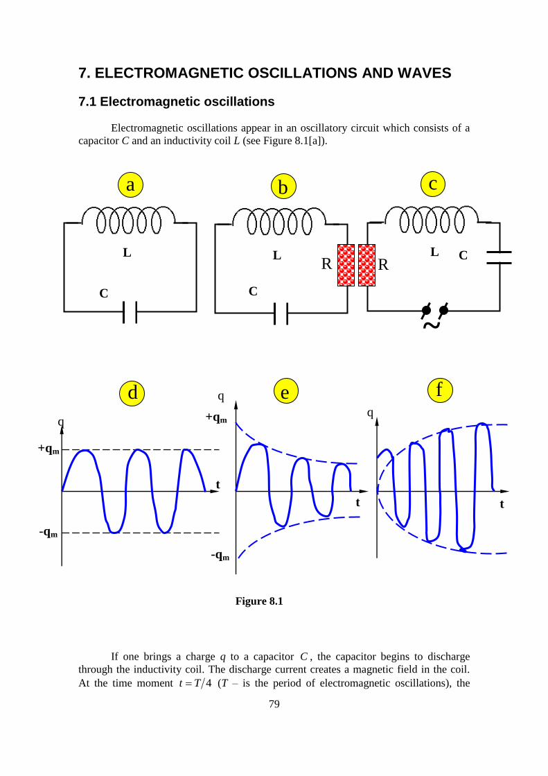
79

7. ELECTROMAGNETIC OSCILLATIONS AND WAVES

7.1 Electromagnetic oscillations

Electromagnetic oscillations appear in an oscillatory circuit which consists of a

capacitor C and an inductivity coil L (see Figure 8.1[a]).

If one brings a charge q to a capacitor C , the capacitor begins to discharge

through the inductivity coil. The discharge current creates a magnetic field in the coil.

At the time moment 4Tt (T – is the period of electromagnetic oscillations), the

+qm

-qm

q

L L L C

C C

R R

a b c

d e f

+qm

t

-qm

t

q

q

t

Figure 8.1

~

80

energy of the electromagnetic field equals zero while the energy of the magnetic field

reaches its maximum value. At a greater time the magnetic field in the coil decreases

and the electric current in the coil is induced. This current again charges the capacitor,

but now its polarity is opposite. At a time moment 2Tt the energy of magnetic field

equals zero, while the energy of electric field reaches its maximal value. At greater

times these processes go on in reverse direction, and at the time moment Tt the

oscillatory circuit returns to its initial state.

Thus, in a circuit exist the oscillations of electric charge at the capacitors plates

(with a period T), the oscillations of the current in a circuit (with a period T) and the

oscillations of the energy of electric and magnetic fields. At the time moments

TTt ,2,0 the energy of the electric field is maximal while the energy of magnetic

field equals zero. At the time moments 43,4 TTt the energy of the magnetic field is

maximal while the energy of the electric field equals zero.

The differential equation describing the free non-damping oscillations in an

oscillatory circuit consisting of an inductivity coil L and a capacitor C (assuming a

resistance R=0) has the form:

02

02

2

qdt

qd , (8.1)

where LC10 - is the self-frequency of undamped oscillations. As a sequence, the

period of oscillations is determined by Thompson’s formula: LCT 22 00 .

The solution of Equation (8.1) is

00sin)( tqtq m , (8.2)

where mq - is the maximal value of a charge on the capacitor’s plate and 0 - is the

initial phase. Using this solution, the current in the oscillatory circuit is defined by the

equation

2/sin)(

)( 00 tIdt

tdqtI m ,

with mm qI 0 being the current amplitude (current maximal value). Using these

solutions for q(t) and I(t), the energy of electric and magnetic fields in the oscillatory

circuit can be written in the following form:

.2cos1

42

cos

2)(

;2cos14

sin22

)(

00

2

00

222

00

2

00

222

tLItLILI

tW

tC

qt

C

q

C

qtW

mmm

mmel

(8.3)

As it follows from Equation (8.3) the values of elW (t) and mW (t) are changing

with the frequency 02 , which is twice as the self-frequency 0 of self-oscillations.

81

If the active resistance R is included into the oscillatory circuit (see Figure

8.1[b]), the damped oscillations of a charge on the capacitor’s plates and damped

oscillations of a current in a circuit occur. In this case the differential equation for the

charge oscillations is as follows:

02 2

02

2

qdt

dq

dt

qd . (8.4)

Equation (8.4) has the solution

0sin)( teqtq t

m , (8.5)

where LR 2 - is the damping coefficient. The frequency and period T of damped

oscillations are determined by the following relations :

22

0 ; 22

0

2

T . (8.6)

As it follows from Equation (8.6), the frequency of damped oscillations is less

than the frequency of free oscillations: 0 , while the period of damped oscillations

is greater than the period of free oscillations, 0TT . When CLR 2 , the process of

a change of the charge at the capacitor’s plates is not the periodic one. Therefore, the

discharge of a capacitor in this case is called non-periodic one. In comparison to free

oscillations, now the maximal values of a charge at capacitor’s plates exponentially

decrease in time, i.e. tqq mm exp , see Figure 8.1(e). The time dependence of the

current in the contour consisting of an active resistance R is described now by equation:

)sin( 0 teII t

m ,

where 2 .

The quantity

TTtq

tq

ln

is called the logarithmic decrement of the damped oscillations. Its physical meaning is

that determines the number of oscillations during the time when the maximal value of

the charge at the capacitor’s plate is decreased by ...71.2e times. Another quantity,

which is often used to characterize the damped oscillations, is the quality factor (Q-

factor) of a circuit. It is defined as

C

L

RQ

1

.

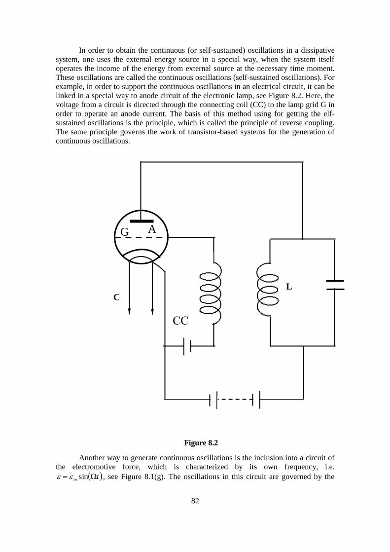
82

In order to obtain the continuous (or self-sustained) oscillations in a dissipative

system, one uses the external energy source in a special way, when the system itself

operates the income of the energy from external source at the necessary time moment.

These oscillations are called the continuous oscillations (self-sustained oscillations). For

example, in order to support the continuous oscillations in an electrical circuit, it can be

linked in a special way to anode circuit of the electronic lamp, see Figure 8.2. Here, the

voltage from a circuit is directed through the connecting coil (CC) to the lamp grid G in

order to operate an anode current. The basis of this method using for getting the elf-

sustained oscillations is the principle, which is called the principle of reverse coupling.

The same principle governs the work of transistor-based systems for the generation of

continuous oscillations.

Another way to generate continuous oscillations is the inclusion into a circuit of

the electromotive force, which is characterized by its own frequency, i.e.

tm sin , see Figure 8.1(g). The oscillations in this circuit are governed by the

СС

G A

C

L

Figure 8.2

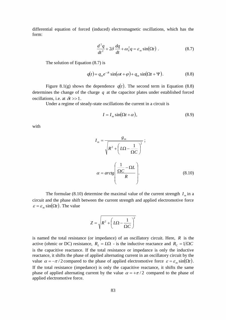
83

differential equation of forced (induced) electromagnetic oscillations, which has the

form:

tqdt

dq

dt

qdm sin2 2

02

2

. (8.7)

The solution of Equation (8.7) is

tqteqtq m

t

m sinsin . (8.8)

Figure 8.1(g) shows the dependence tq . The second term in Equation (8.8)

determines the change of the charge q at the capacitor plates under established forced

oscillations, i.e. at 1t .

Under a regime of steady-state oscillations the current in a circuit is

tII m sin , (8.9)

with

2

2 1

CLR

gI m

m ;

R

LCarctg

1

. (8.10)

The formulae (8.10) determine the maximal value of the current strength mI in a

circuit and the phase shift between the current strength and applied electromotive force

tm sin . The value

2

2 1

CLRZ

is named the total resistance (or impedance) of an oscillatory circuit. Here, R is the

active (ohmic or DC) resistance, LRL - is the inductive reactance and CRC 1

is the capacitive reactance. If the total resistance or impedance is only the inductive

reactance, it shifts the phase of applied alternating current in an oscillatory circuit by the

value 2/ compared to the phase of applied electromotive force tm sin .

If the total resistance (impedance) is only the capacitive reactance, it shifts the same

phase of applied alternating current by the value 2/ compared to the phase of

applied electromotive force.

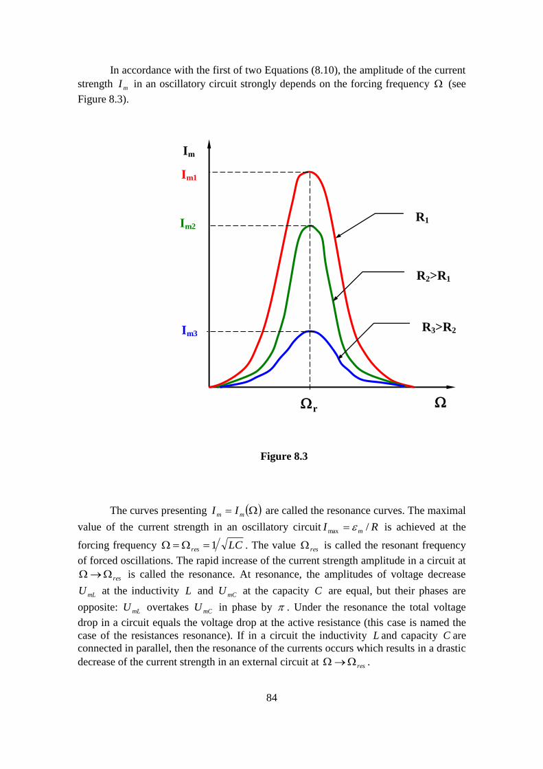
84

In accordance with the first of two Equations (8.10), the amplitude of the current

strength mI in an oscillatory circuit strongly depends on the forcing frequency (see

Figure 8.3).

The curves presenting mm II are called the resonance curves. The maximal

value of the current strength in an oscillatory circuit RI m /max is achieved at the

forcing frequency LCres 1 . The value res is called the resonant frequency

of forced oscillations. The rapid increase of the current strength amplitude in a circuit at

res is called the resonance. At resonance, the amplitudes of voltage decrease

mLU at the inductivity L and mCU at the capacity C are equal, but their phases are

opposite: mLU overtakes mCU in phase by . Under the resonance the total voltage

drop in a circuit equals the voltage drop at the active resistance (this case is named the

case of the resistances resonance). If in a circuit the inductivity L and capacity C are

connected in parallel, then the resonance of the currents occurs which results in a drastic

decrease of the current strength in an external circuit at res .

Im

Im1

Im2

Im3

r

R2>R1

R1

R3>R2

Figure 8.3

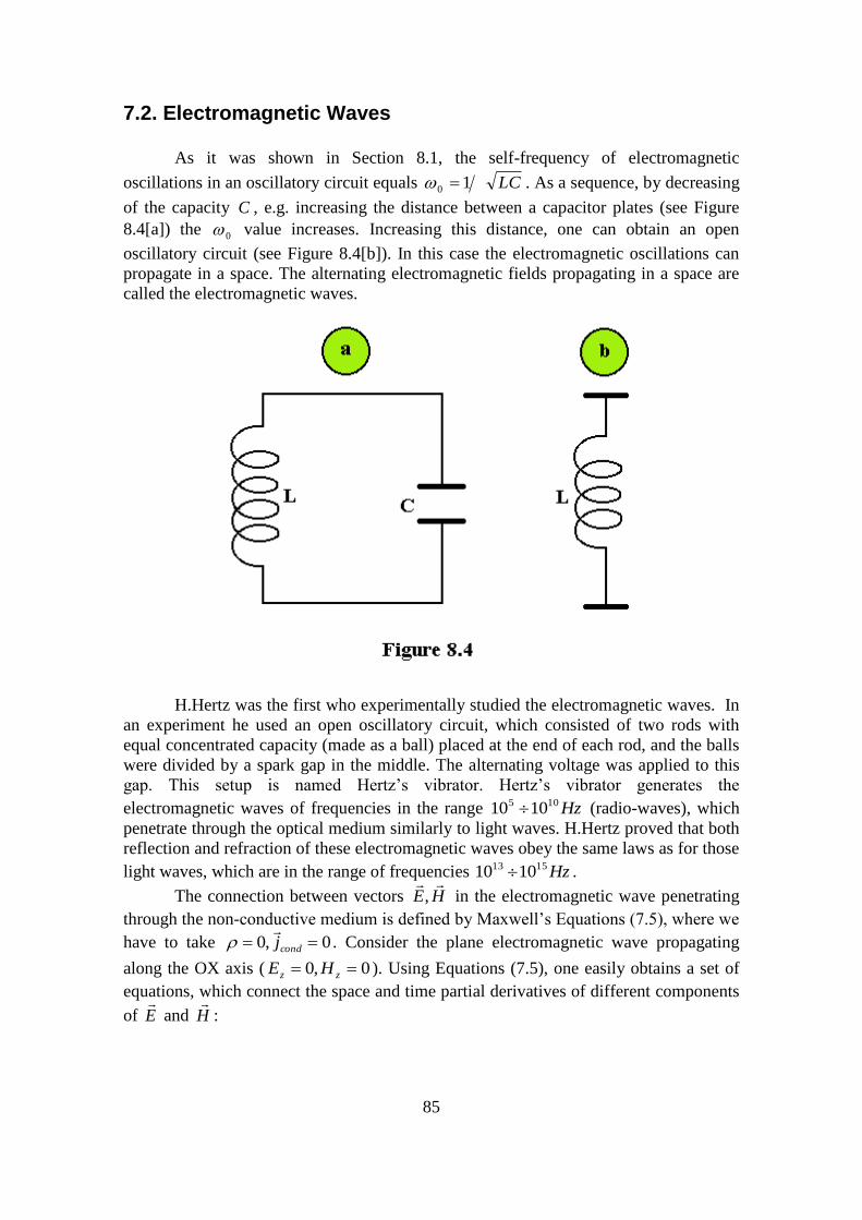
85

7.2. Electromagnetic Waves

As it was shown in Section 8.1, the self-frequency of electromagnetic

oscillations in an oscillatory circuit equals LC10 . As a sequence, by decreasing

of the capacity C , e.g. increasing the distance between a capacitor plates (see Figure

8.4[a]) the 0 value increases. Increasing this distance, one can obtain an open

oscillatory circuit (see Figure 8.4[b]). In this case the electromagnetic oscillations can

propagate in a space. The alternating electromagnetic fields propagating in a space are

called the electromagnetic waves.

H.Hertz was the first who experimentally studied the electromagnetic waves. In

an experiment he used an open oscillatory circuit, which consisted of two rods with

equal concentrated capacity (made as a ball) placed at the end of each rod, and the balls

were divided by a spark gap in the middle. The alternating voltage was applied to this

gap. This setup is named Hertz’s vibrator. Hertz’s vibrator generates the

electromagnetic waves of frequencies in the range Hz105 1010 (radio-waves), which

penetrate through the optical medium similarly to light waves. H.Hertz proved that both

reflection and refraction of these electromagnetic waves obey the same laws as for those

light waves, which are in the range of frequencies Hz1513 1010 .

The connection between vectors HE

, in the electromagnetic wave penetrating

through the non-conductive medium is defined by Maxwell’s Equations (7.5), where we

have to take 0,0 condj

. Consider the plane electromagnetic wave propagating

along the OX axis ( 0,0 zz HE ). Using Equations (7.5), one easily obtains a set of

equations, which connect the space and time partial derivatives of different components

of E

and H

:

86

t

H

x

Ezy

0 ;

t

H

x

E yz

0 ;

t

E

x

Hzy

0 ; .0

t

E

x

H yz

(8.11)

From the set of Equations (8.11) one obtains the wave equations for the

components of the vectors E

and H

of the plane electromagnetic wave:

2

2

0022

2

t

E

x

E yy

:

2

2

002

2

t

H

t

H zz

. (8.12)

The comparison of Equations (8.12) and (7.6) leads to the conclusion that the

plane electromagnetic wave can be completely defined using only the vector potential

.

Indeed,

krotE

,1

00

,

here k

- is the unit vector directed along the propagation of electromagnetic wave. The

velocity of this wave is

00

1v . (8.13)

Here, scmc /1031 9

00 is the speed of light in a vacuum. Therefore, the

velocity of electromagnetic wave given by Equation (8.13) is rewritten now in the form:

n

ccv

, (8.14)

where n - is the refractive index of a medium through which an electromagnetic wave

propagates. The coincidence of Equation (8.14) with similar equation in the optics let us

make a conclusion (J.C.Maxwell): the light waves are the electromagnetic waves. From

Equations (8.12) it follows also that the vectors E

and H

are mutually perpendicular

and are perpendicular to the velocity vector v

of a wave, see Figure 8.5. Therefore, the

light is the electromagnetic transverse waves. In these waves the vectors E

, H

always

oscillate in the same phases, and their values at the arbitrary point of a space are

connected through equation

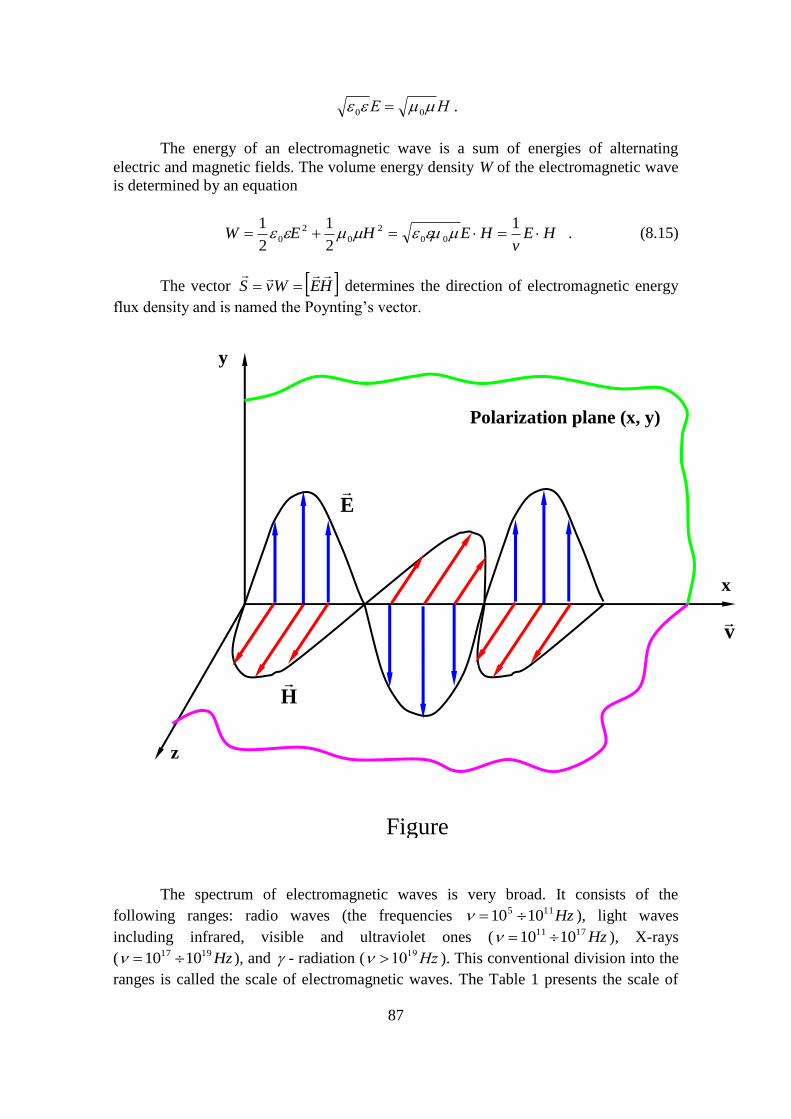
87

HE 00 .

The energy of an electromagnetic wave is a sum of energies of alternating

electric and magnetic fields. The volume energy density W of the electromagnetic wave

is determined by an equation

HEv

HEHEW 1

2

1

2

100

2

0

2

0 . (8.15)

The vector HEWvS

determines the direction of electromagnetic energy

flux density and is named the Poynting’s vector.

The spectrum of electromagnetic waves is very broad. It consists of the

following ranges: radio waves (the frequencies Hz115 1010 ), light waves

including infrared, visible and ultraviolet ones ( Hz1711 1010 ), X-rays

( Hz1917 1010 ), and - radiation ( Hz1910 ). This conventional division into the

ranges is called the scale of electromagnetic waves. The Table 1 presents the scale of

Polarization plane (x, y)

H

E

v

x

y

z

Figure

8.5

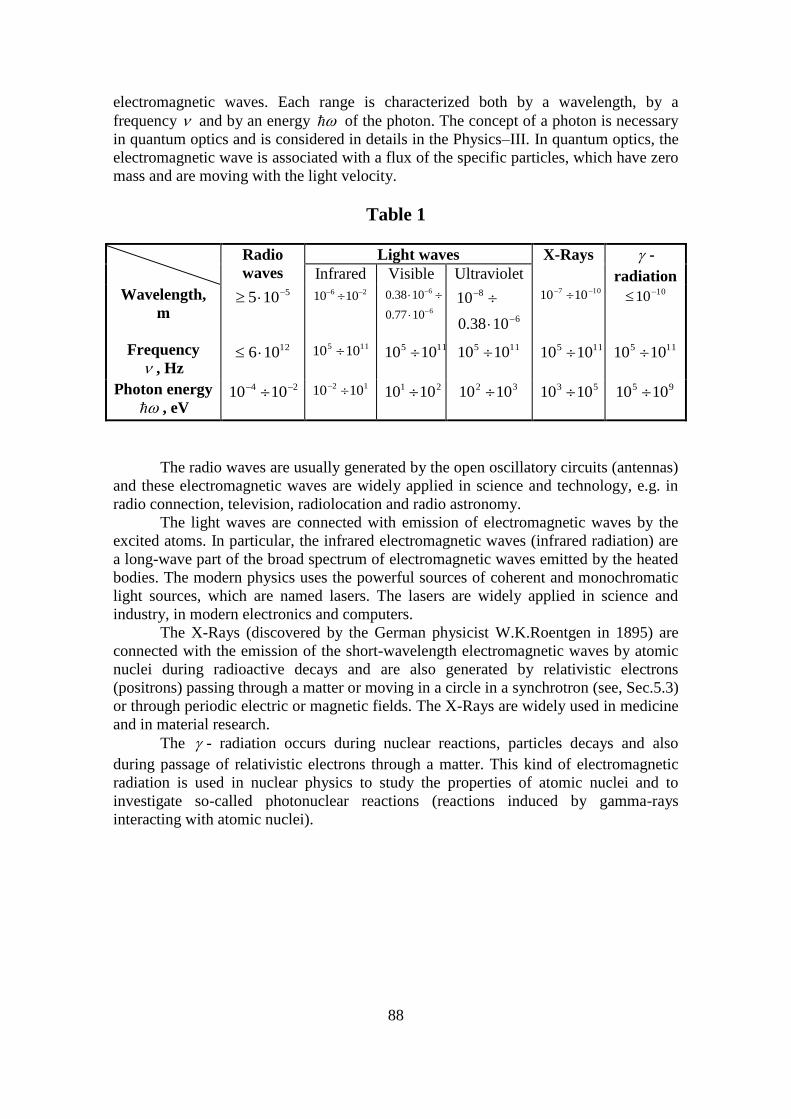
88

electromagnetic waves. Each range is characterized both by a wavelength, by a

frequency and by an energy of the photon. The concept of a photon is necessary

in quantum optics and is considered in details in the Physics–III. In quantum optics, the

electromagnetic wave is associated with a flux of the specific particles, which have zero

mass and are moving with the light velocity.

Table 1

Radio

waves

Light waves X-Rays -

radiation Infrared Visible Ultraviolet

Wavelength,

m

5105 26 1010

6

6

1077.0

1038.0

6

8

1038.0

10

107 1010

1010

Frequency

, Hz

12106 115 1010 115 1010

115 1010 115 1010

115 1010

Photon energy

, eV

24 1010

12 1010 21 1010

32 1010 53 1010

95 1010

The radio waves are usually generated by the open oscillatory circuits (antennas)

and these electromagnetic waves are widely applied in science and technology, e.g. in

radio connection, television, radiolocation and radio astronomy.

The light waves are connected with emission of electromagnetic waves by the

excited atoms. In particular, the infrared electromagnetic waves (infrared radiation) are

a long-wave part of the broad spectrum of electromagnetic waves emitted by the heated

bodies. The modern physics uses the powerful sources of coherent and monochromatic

light sources, which are named lasers. The lasers are widely applied in science and

industry, in modern electronics and computers.

The X-Rays (discovered by the German physicist W.K.Roentgen in 1895) are

connected with the emission of the short-wavelength electromagnetic waves by atomic

nuclei during radioactive decays and are also generated by relativistic electrons

(positrons) passing through a matter or moving in a circle in a synchrotron (see, Sec.5.3)

or through periodic electric or magnetic fields. The X-Rays are widely used in medicine

and in material research.

The - radiation occurs during nuclear reactions, particles decays and also

during passage of relativistic electrons through a matter. This kind of electromagnetic

radiation is used in nuclear physics to study the properties of atomic nuclei and to

investigate so-called photonuclear reactions (reactions induced by gamma-rays

interacting with atomic nuclei).