PHYSICS DEPARTMENT’ - · PDF filePHYSICS DEPARTMENT’ ’ ’...
139
PHYSICS DEPARTMENT Heat Transport in Evacuated Perlite Powder Insulations and Its Application in LongTerm Hot Water Storages Master Thesis of Matthias Demharter TECHNISCHE UNIVERSITÄT MÜNCHEN
Transcript of PHYSICS DEPARTMENT’ - · PDF filePHYSICS DEPARTMENT’ ’ ’...

PHYSICS DEPARTMENT
Heat Transport in Evacuated Perlite Powder Insulations and Its Application in Long-‐Term
Hot Water Storages
Master Thesis of
Matthias Demharter
TECHNISCHE UNIVERSITÄT
MÜNCHEN


Heat Transport in Evacuated Perlite Powder Insulations and Its
Application in Long-Term Hot Water Storages
Master Thesis
of
Matthias Demharter
Technische Universität München
Physics Department
Supervisor: Prof. Dr. Rudolf Gross
Bavarian Center for Applied Energy Research (ZAE Bayern)
Division 1: Technology for Energy Systems and Renewable Energy
Advisor: Dr. Thomas Beikircher
Garching, August 2011

.

iii
Abstract
For many years, the technique of vacuum super insulation (VSI) with expanded perlitehas been used for cryogenic applications, especially the storage of liquid gases at temper-atures of 20K ≤ T ≤ 90K. Expanded perlite is an amorphous, highly porous, granularmaterial of volcanic origin. Its two main components are SiO2 (70 %) and Al2O3 (15 %).Due to the small pore diameters and the small distances between the grains, gas con-duction in the pores and in the intergranular spaces is suppressed already in the regimeof fine vacuum (p ≈ 0.01mbar). As a consequence of the material structure, solid con-duction is inhibited to a great extent. Furthermore, thermal radiation is blocked by theopaque solid.
Due to these properties and as a consequence of the temperature dependency of theradiative heat transport, which scales with T
4, effective thermal conductivities as lowas 3 to 5 · 10−3 W/mK have been realized at cryogenic temperatures. Compared to con-ventional insulation materials like polyurethane or rock wool at ambient temperature,the thermal conductivity is lowered by a factor of 6 to 10. A commercially availabletype of expanded perlite is TECHNOPERL ® - C 1,5 from the Austrian manufacturerEUROPERL, STAUSS PERLITE GMBH. This specific material is actually used in practicefor liquid gas storage tanks.
In a current federally granted research project at ZAE Bayern (grant number 0325964A,German ministry of environment), the approach is pursued to apply perlite based VSIalso at higher temperatures. Primarily, the long-term and seasonal storage of hot wa-ter up to T = 150 °C in solar thermal heating systems is considered. However, otherfields of application have also been identified, for example the intermediate storageof thermal energy in industrial processes or in solar thermal power plants for electricpower generation. So far, experimental data for the effective thermal conductivity λeff
of evacuated perlite in this temperature regime has been very rare. Therefore, vari-ous measurements have been performed within this thesis in order to determine λeff
of TECHNOPERL ® - C 1,5 at different temperatures (20 °C ≤ T ≤ 150 °C), vacuumpressures (10−3 mbar ≤ p ≤ 103 mbar), densities (55kg/m³ ≤ ρ ≤ 95kg/m³) and grainstructures (self-compression of the bulk by space-saving arrangement in a close-packingof spheres on the one hand versus application of external mechanical pressure, result-ing in partial grain destruction on the other hand). Laboratory experiments have been

iv Abstract
done both in an existing parallel plate apparatus and in a cut-off cylinder device, whichwas specially designed and set up during this thesis. In order to separately determinethe radiative heat transport, Fourier transform infrared spectroscopy (FTIR) measure-ments have been performed and evaluated. Furthermore, a real-size cylindrical storageprototype with a water storage volume of V = 16.4m³ has been available for experimentsunder practical conditions.
In order to interpret and compare the measurement data, a theoretical understandingof the different heat transport mechanisms contributing to the effective thermal con-ductivity of evacuated perlite has been developed, and it has been possible to explainthe results of all four measurements in a consistent way. For this theoretical descrip-tion, conventional approaches and models have been used, which have successfully beenapplied to similar systems during the last decades, and which can be found in litera-ture: The pressure dependency of gaseous conduction has been characterized using theSherman interpolation between the continuum at high pressures and the regime of freemolecular flow at low pressures. Regarding the solid thermal conductivity, a linear de-pendency on density has been derived from the experimental data. This result is inagreement with other empirical findings. However, the initially assumed dependencyof solid conduction on temperature has not been observable. Radiative heat transporthas been treated using the heat diffusion model, which describes absorption and scat-tering of thermal radiation within a material and allows the introduction of a radiativethermal conductivity. For the gas conduction in the intergranular spaces, also referredto as coupling effect, a special new model for perlite has been developed, based on ap-proaches, which have originally been applied to particle beds in general, and have alsobeen adapted to aerogels in particular.
For gaseous conduction inside the pores, the experimentally determined characteris-tic half-value pressure for air ranges from p
g1/2 = 1.38mbar to p
g1/2 = 5.1mbar. These
values correspond to effective mean pore diameters of dp = 167µm and dp = 45.1µm.Similar results have been obtained from measurements with the inert gases argon(pg1/2 = 1.46mbar) and krypton (pg1/2 = 1.24mbar). For the coupling term, a half-valuepressure of pc1/2 = 39mbar has been derived from the measurements with air. This re-sult is equivalent to an effective grain interspace of dg = 5.9µm. For argon and krypton,the respective values are p
c1/2 = 17.4mbar (argon) and p
c1/2 = 4.5mbar (krypton). This
might indicate that the interaction of the heavy noble gases with the perlite surface isdifferent from the diatomic air molecules N2 and O2.
For practical purposes, simple formulas have been derived to calculate the effectivethermal conductivity λeff of TECHNOPERL ® - C 1,5 and its individual componentsλr (radiative heat transport), λs (solid conduction), λg (gas conduction in pores) and λc
(coupling effect) as a function of vacuum pressure (including the filling gases air, argonand krypton), bulk density and temperature. This knowledge is of particular interest

Abstract v
for the application of vacuum super insulation in practice. From the theoretical modelsand the experimental results, it has been possible to suggest optimization approaches tominimize λeff . Currently, a value as low as λeff = 9.2 · 10−3 W/mK has been achieved forthe real-size prototype at a mean water temperature of T = 86.4 °C, which is composedof λr = 2.6 · 10−3 W/mK, λs = 5.1 · 10−3 W/mK and λg + λc = 1.5 · 10−3 W/mK. By using abulk density of around ρ = 60kg/m³ and lowering the vacuum pressure to p = 0.01mbar,this value is expected to decrease to λeff ≈ 7.3 · 10−3 W/mK according to the theoreticalpredictions. The application of inert filling gases like argon or krypton has been provento be disadvantageous.
A further experimental task was the determination of the moisture content withinTECHNOPERL ® - C 1,5. According to theory, moisture in its liquid or gaseous form candramatically increase the thermal conductivity of an insulation in some cases. However,as a result of the experiments and due to phase diagram considerations, these effectscan be neglected for practical applications.

vi
Contents
1 Introduction 1
1.1 Motivation and Background . . . . . . . . . . . . . . . . . . . . . . . . . . . 1
1.2 Definition of Tasks and Goals . . . . . . . . . . . . . . . . . . . . . . . . . . 7
1.3 Structure and Procedure . . . . . . . . . . . . . . . . . . . . . . . . . . . . . 7
2 Fundamentals of Heat Transport 9
2.1 Conduction . . . . . . . . . . . . . . . . . . . . . . . . . . . . . . . . . . . . . 9
2.2 Convection . . . . . . . . . . . . . . . . . . . . . . . . . . . . . . . . . . . . . 11
2.3 Radiation . . . . . . . . . . . . . . . . . . . . . . . . . . . . . . . . . . . . . . 14
3 Overview: Insulation Techniques 17
3.1 Conventional Insulation Materials . . . . . . . . . . . . . . . . . . . . . . . 17
3.2 Vacuum Insulation . . . . . . . . . . . . . . . . . . . . . . . . . . . . . . . . 18
3.3 Vacuum Super Insulation . . . . . . . . . . . . . . . . . . . . . . . . . . . . 20
3.3.1 Foil Insulation . . . . . . . . . . . . . . . . . . . . . . . . . . . . . . . 20
3.3.2 Powder Insulation . . . . . . . . . . . . . . . . . . . . . . . . . . . . . 22
4 Heat Transport in Evacuated Powder Insulations 23
4.1 Gas Heat Conduction and Smoluchowski Effect . . . . . . . . . . . . . . . . 23
4.2 Solid Heat Conduction . . . . . . . . . . . . . . . . . . . . . . . . . . . . . . 30
4.3 Radiative Heat Transfer . . . . . . . . . . . . . . . . . . . . . . . . . . . . . 32
4.4 Coupling Effect . . . . . . . . . . . . . . . . . . . . . . . . . . . . . . . . . . 36
4.5 Effective Thermal Conductivity . . . . . . . . . . . . . . . . . . . . . . . . . 39
4.6 Influences of Moisture . . . . . . . . . . . . . . . . . . . . . . . . . . . . . . 40

Contents vii
5 Perlite and Vacuum Super Insulation: State of the Art 45
5.1 General Properties of Perlite . . . . . . . . . . . . . . . . . . . . . . . . . . . 45
5.2 Vacuum Super Insulation in Cryogenic Engineering . . . . . . . . . . . . . 47
5.3 Vacuum Super Insulation of District Heating Pipelines . . . . . . . . . . . 48
5.4 Vacuum-Super-Insulated Panels in Civil Engineering . . . . . . . . . . . . 49
5.5 Material Selection and Motivation for Additional Research . . . . . . . . . 50
6 Laboratory Measurements Regarding the Heat Conductivityof Evacuated Perlite 53
6.1 Spectroscopic Determination of The Radiative Thermal Conductivity . . . 53
6.1.1 Principles of FTIR Spectroscopy . . . . . . . . . . . . . . . . . . . . . 54
6.1.2 Measurement Procedure . . . . . . . . . . . . . . . . . . . . . . . . . 56
6.1.3 Experimental Results . . . . . . . . . . . . . . . . . . . . . . . . . . . 56
6.2 Effective Thermal Conductivity Measurements in a Parallel Plate Setup . 59
6.2.1 Measurement Setup and Experimental Procedure . . . . . . . . . . 59
6.2.2 Presentation and Evaluation of Measurement Results . . . . . . . . 61
6.3 Measurements in a Cut-Off Cylinder Apparatus . . . . . . . . . . . . . . . 67
6.3.1 Conception, Setup and Procedure of the Experiment . . . . . . . . . 67
6.3.2 Presentation and Discussion of Measurement Results . . . . . . . . 73
6.4 Determination of the Moisture Content . . . . . . . . . . . . . . . . . . . . 86
7 Heat Loss Measurements on a Real-Size Storage Prototype 89
7.1 Tank Layout and Measurement Setup . . . . . . . . . . . . . . . . . . . . . 89
7.2 Presentation and Evaluation of Measurement Results . . . . . . . . . . . . 92
8 Summary of the Experimental Results and Conclusions 103
8.1 Calculation of the Effective Thermal Conductivity for Practical Purposes . 103
8.2 Suggestion of Optimization Approaches . . . . . . . . . . . . . . . . . . . . 106
9 Outlook 113

.

1
Chapter 1
Introduction
1.1 Motivation and Background
During the last years, renewable energy sources have continuously gained importance(figure 1.1). In Germany, roughly 10 % of the overall energy demand are meanwhilesupplied from renewables [1]. As one of the pioneering nations regarding the expansionof renewable energies, the German government has declared the intent to increase thisfraction to 18 % until 2020 and to 50 % by 2050 [2]. Also in other countries, there areinitiatives to expand the usage of renewable energies. This development is mainly mo-tivated by the ambition of climate protection. In general, an increasing awareness forsustainability has been observed in our society during the last years [3]. Especially nu-clear energy has dramatically lost its acceptance as a consequence of the recent series ofaccidents at the Fukushima nuclear power plant [4]. The nuclear power phase-out until2022, which was subsequently decided by the German government [5], is planned to berealized by enhanced application of renewable energies.
Figure 1.1: Contribution of renewables to the supply of final energy in Germany [1].

2 Chapter 1. Introduction
However, the change from conventional energy sources to renewables can not be accom-plished just by political decisions and societal trends. Economic factors also play animportant role. In many cases, burning fossil fuels for heating and electric power gener-ation is still favorable from the economic point of view, not to mention automotive andtransport applications. Nevertheless, because the availability of fossil fuels is begin-ning to decrease [6] and prices have steadily been rising (figure 1.2) [7], the break-evenpoint might soon be reached. Due to the recent introduction of CO2 emissions trading[8], renewable energy sources will be more competitive in future. In both the economicand environmental context, also the terms of energy saving and energy efficiency havegained a greater significance.
Even in an industrialized country like Germany, the supply of hot water for domestic useand residential heating makes up a considerable fraction of approximately 20 % [9] ofthe total energy demand (compare also figure 1.3). Most heating systems are still basedon fossil fuels like oil or gas, but there is a huge potential to provide the energy requiredfor this purpose from renewable sources. Modern solar thermal systems [10, 11] havebecome an economically reasonable alternative, not to mention environmental factorslike reduction of CO2 emissions.
Figure 1.2: Development of the crude oil price in US Dollar per barrel [12].
Figure 1.3: Energy demand profile of Germany in 2007 [7].

1.1. Motivation and Background 3
A solar thermal system for single-family houses (figure 1.4) basically consists of a collec-tor and a storage. The essential component of any collector is the absorber, which heatsup as it absorbs the incoming solar radiation. For simple and economic collectors, theemissivity ε (and thus also the absorptivity α, see section 2.3) of the absorber surfaceis typically close to 1 in the whole spectral range. Modern absorbers in high-efficiencycollectors have a selective coating with a high emissivity only in the range of incomingradiation and a low emissivity in the infrared regime in order to reduce losses from re-emission [13]. The heat emerging at the absorber is led away by the heat carrier, oftena mixture of water and glycol for frost protection, which flows through the collector. Theexisting types of collectors basically only differ from each other regarding the insulationtechniques that are applied in order to reduce thermal losses. Due to this, also the geo-metrical layout varies. Free convection is usually suppressed by glass covers. Commonflat plate collectors are additionally insulated with mineral wool or similar materials ontheir rear side and reach efficiencies of 50 - 60 % at typical operation temperatures be-tween 50 and 80 °C [14, 15]. Evacuated tube collectors utilize the insulating propertiesof vacuum to obtain higher efficiencies at operation temperatures up to 120 °C.
Since solar irradiation is not constantly available, thermal storages are fundamentallyimportant for solar thermal systems. A typical storage tank is built in a slim, cylindricallayout. Due to the the temperature dependency of the density of water, this designallows the development of a stable temperature gradient to maximize the storage exergy.The water at the bottom of the tank is colder and thus heavier than the hotter waterlayered further above. To charge the storage with the heat coming from the collector, aheat exchanger is installed at the cold bottom of the tank. Hence, the temperature ofthe heat carrier fluid running back into the collector circuit reaches a lower level, whichis more beneficial for the overall efficiency of the system [14]. The connections for theextraction of hot water are located in the upper part of the tank to ensure water supplywith the hottest possible temperature.
Figure 1.4: System overview of a solar thermal heating installation [14].

4 Chapter 1. Introduction
An important component of any storage is its insulation, which reduces the thermallosses of the stored hot water to its colder surroundings. At present, storages are insu-lated using conventional materials like mineral wool or polyurethane foam. The heatconductivity λ of these materials (at room temperature) is typically between 0.024 and0.05 W/mK.
Most of today’s solar thermal installations are only used to produce hot water for domes-tic use. Only a minority of installed facilities also supports residential heating. Witha collector area of 10 - 20 m² and storage sizes between 500 and 1500 liters [16], suchsystems can provide around 20 - 30 % of the total heat demand of a single-family house(solar fraction). The remaining bigger part must still be supplied by fossil fuels. Adetailed investigation using numerical simulation methods [17] shows, that the solarfraction can be improved not only by lowering the heat conductivity of the insulation,but also by increasing the storage volume to 10 - 20 m³ (assuming reasonably-sized col-lectors). In this way it is possible to transfer the thermal energy generated at days withhigh solar irradiation into colder periods. Due to this long-time storage, solar fractionsof more than 50 % are possible (fossil-supported solar heating). In the extreme case, theheat generated in summer can be carried over into the winter months. This conceptis referred to as seasonal storage and allows solar fractions of up to 100 % (completesolar coverage). However, seasonal storage requires storage volumes of around 100 m³and higher. So far, the number of solar thermal installations with such large storagesand solar fractions greater than 50 % has been very low (only around 100 buildings inGermany [18]), although lately more and more manufacturers offer conventionally in-sulated tanks with volumes of several m³ for long-time storage [19, 20].
From a general consideration of the thermal energy storage process, some importantprinciples for practical applications can be derived. The temperature T of the storagemedium (initial temperature T0) decreases with time t as a consequence of the thermallosses Q to the colder surroundings (ambient temperature Ta). On the one hand, Q isconnected to the temperature decrease dT/dt by the integral heat capacity C = cpρV ofthe storage medium (cp: specific heat capacity, ρ: density, V : storage volume). On theother hand, Q can be expressed by λA (T − Ta) /d (λ: heat conductivity of the insula-tion, A: tank surface, d: insulation thickness). After solving the emerging differentialequation, the evolution of T (t) can be calculated:
λA
d(T − Ta) = Q = −C
dT
dt= −cpρV
dT
dt
dT
T − Ta= − Aλ
cpρV ddt
ln
T − Ta
T0 − Ta
= − Aλ
cpρV dt
T (t) = (T0 − Ta) exp
− Aλ
cpρV dt
+ Ta (1.1)
1.1. Motivation and Background 5
On a sidenote, the relation Q = λA (T − Ta) /d is an approximation, which is only valid ifthe insulation thickness is much smaller than the radius of the cylindrical tank (d r,see section 2.1 for details). For practical applications, it is desired to keep the constantAλ/cpρV d, which determines the cooling rate, as small as possible. Because ρ and cp arenatural properties of water, this can be achieved by three different approaches:
• A first possibility is to minimize the ratio A/V , which can be done by building largestorage tanks. This result is in good agreement with the numerical simulationsmentioned above, which showed that an up-scaling of the tank dimensions yieldshigher solar fractions. In addition, spherically-shaped storage tanks are most fa-vorable regarding the ratio A/V . The cylindrical geometry is more practical inmany applications, though.
• Furthermore, the cooling rate can be lowered by increasing the insulation thick-ness d. However, this method is limited by spatial restrictions. In practice, it isdesired to obtain a reasonable ratio of storage volume against total tank volume.
• A third method is to use insulation materials and techniques which yield low ther-mal conductivities. This approach is pursued in this thesis.
In this context, a new super-insulated long-term hot water storage is being developed atthe Bavarian Center for Applied Energy Research (ZAE BAYERN) in cooperation withHUMMELSBERGER GMBH, a medium-sized company in the branch of steel processing.The project is funded by the German Federal Environment Ministry [2]. The cylindricaltanks can be built in sizes between 5 and 100 m³. A particular feature is the applicationof vacuum super insulation. This technique is known from cryogenic engineering and isnow used in solar thermal applications for the first time. By evacuating a microporouspowder, all possible heat transfer mechanisms are effectively suppressed and in princi-pal, thermal conductivities as low as 0.005 W/mK can be reached [17, 21]. The materialused for this purpose is perlite, a porous compound of volcanic origin.
In general, the newly-developed storage tank can be applied to any kind of thermal en-ergy storage process. From storage efficiency considerations, it is obvious though thatan improvement of the thermal insulation is especially important for long storage du-rations and for high temperature levels (compare equation 1.1). Thus, one can identifythe following main fields of application for the new super-insulated tank:
First, the long-term storage of solar thermal energy as described above is considered.Due to T < 100 °C, this represents an application at relatively low temperatures, butlong storage durations. With maximum possible tank volumes of 100 m³, seasonal stor-age is also possible. For conventional solar thermal applications, the storage can beequipped with a special stratification device, which ensures that the water coming fromthe collector is inserted at the appropriate height according to its temperature. In thisway, the temperature gradient can be kept stable, and a mixing of the different temper-atures is prevented.

6 Chapter 1. Introduction
Moreover, one can also think of the intermediate storage of industrial process heat toimprove the energy efficiency and to lower production costs. Roughly a third of the pro-cess heat demand is in the temperature range below 250 °C [22]. Relevant branches arefor example the chemical industry, food industry and paper production. At this temper-ature level, pressurized water is a suitable storage medium. With recently developedcollectors [23], heat at this temperature range (T ≈ 150 °C) can even be supplied bysolar thermal systems.
Higher temperatures from 300 °C of up to 1600 °C are mainly needed for mineral oiland metal processing and for some processes in chemical industry. If it is possible toimplement intermediate storage for these processes, their energy efficiency could beconsiderable increased, because vacuum super insulation is especially advantageousat these high storage temperatures. However, as a small restriction, the maximumtemperature is limited, because the amorphous, glass-like perlite can not withstandtemperatures above 800 °C. Furthermore, alternative storage media (e.g. molten salts)would have to be used.
As a third field of application, solar thermal power plants for electric power generationcan be mentioned [24, 25]. For large-scale applications in the range of 10 to 50 MW, twodifferent concepts can be distinguished. With parabolic trough collectors (figure 1.5 a),the incident solar radiation is concentrated on a focal line. Concentration factors ofaround 80 and temperatures close to 400 °C can be reached. Even higher temperaturesare possible with solar towers (figure 1.5 b), which are also called central receiver sys-tems (CRS). Here, an arrangement of reflectors (heliostats) is used to concentrate thesolar radiation to a small volume at the central receiver, which is located on top of a sta-tionary tower. Concentration factors of 500 to 1000 and temperatures of up to 1100 °Ccan be achieved as a consequence of the two-dimensional concentration. The theoreti-cal limit is given by T = 5777K, which is the surface temperature of the sun. In bothconcepts, conventional turbines are used to generate electricity.
Figure 1.5: Parabolic trough collector at the National Solar Energy Center in Israel (a),Gemasolar CRS power plant in Fuentes de Andalucía, Spain (b) [26, 27].

1.2. Definition of Tasks and Goals 7
Figure 1.6: System overview of a solar thermal power plant with thermal storage [25].
The implementation of intermediate thermal storage is possible for both systems andhas already been realized (figure 1.6). In this way, excess heat can be stored during theday, and the power plant can continue to generate electricity after sunset. For example,the operation time can be extended by an interval of up to 7 hours in some parabolictrough plants in Spain. With a combination of collectors, storages and turbines of ap-propriate sizes, configurations for base load, medium load and peak load supply can beset up. In the relevant temperature regime, molten salts are often used as a storagemedium. With the application of vacuum super insulation, which is especially advanta-geous at high temperatures, the efficiency of the storage process can be increased.
1.2 Definition of Tasks and Goals
The primary aim of this thesis is the theoretical and experimental investigation of theheat transport in an evacuated perlite powder insulation. This includes both the quan-tification of the overall heat conductivity and the analysis of different heat transportmechanisms as a function of pressure, temperature and density. Based on this funda-mental understanding, another goal is to examine how the total thermal conductivitycan be minimized under economical aspects in practice, and to formulate optimizationapproaches for the application in long-term hot water storages.
1.3 Structure and Procedure
In the first part of this report, the physical and technical background of vacuum superinsulation is depicted. After a short overview about heat transport in general (chap-ter 2) and a brief presentation of existing insulation techniques (chapter 3), the theory

8 Chapter 1. Introduction
of heat transport in the special case of evacuated powders is investigated in chapter 4.Subsequently, the material perlite and its general properties are treated (chapter 5).Apart from the cryogenic application mentioned above, vacuum super insulations havealso been developed for civil engineering applications. Furthermore, the technology hasbeen considered and examined for long-distance heating pipelines. Therefore, chapter 5also presents the state of scientific and technical knowledge for these applications andmotivates the additional research done in this thesis.
The second part is about the performed experiments. Laboratory measurements (chap-ter 6) have been done in order to provide a general understanding of the heat transportmechanisms of evacuated perlite. In addition, the influence of inert filling gases on thethermal conductivity has been analyzed, and the moisture content of the material hasbeen determined. In order to examine whether the results from laboratory experimentsremain valid under practical conditions, heat loss measurements have been performedon a real-size storage prototype (chapter 7). Both experimental chapters contain thedescription of the respective measurement setup and procedure as well as the presen-tation and discussion of results. Eventually, chapter 8 summarizes the experimentalresults with regard to the practical application of vacuum super insulation in hot waterstorages and outlines optimization approaches.

9
Chapter 2
Fundamentals of Heat Transport
Generally speaking, heat is the form of energy which can be transferred between ther-modynamic systems as a consequence of a temperature difference [28]. Three differentmechanisms of heat transport can be distinguished: conduction, convection and radia-tion. The following sections will briefly describe each of them and focus on equationsthat will be used in the further progression of this thesis. More detailed explanationscan be found in relevant textbooks [10, 28, 30, 31, 32, 33].
2.1 Conduction
Conduction is a heat transfer mechanism that is based on the direct interaction betweenparticles (atoms, molecules, electrons, phonons) and can occur in any kind of matter.Unlike radiation, conduction requires a medium, but no bulk movement of particles. Ingases and liquids, the atoms or molecules are mobile, and conduction happens due tocollisions of the particles along their random walk. In solids, by contrast, the atomsare bound in a lattice, and conduction is a result of vibrations, physically described byphonons. Additionally, there can be a contribution of free electrons.
Consider a homogeneous, arbitrarily-shaped, three-dimensional body composed of anisotropic material with a temperature distribution T (x). In the stationary case, heatconduction can be mathematically expressed by Fourier’s law. In its differential form itreads
−→q = −λ∇T (2.1)
where −→q is the local heat flux per unit area, ∇T is the temperature gradient and the
constant of proportionality λ is the thermal conductivity of the material. This equationshows very descriptively that a heat flux is caused by a temperature gradient and thatthe flux in a certain direction is proportional to the temperature gradient in that spe-cific direction. The negative sign expresses that heat flux is always directed towardsdecreasing temperatures.

10 Chapter 2. Fundamentals of Heat Transport
For simple geometries, Fourier’s law can be reduced into its one-dimensional form:
Q = −AλdT
dr(2.2)
Here, the gradient ∇T is replaced by the one-dimensional derivative dT/dr and the areaA is introduced, which is always aligned normally to the direction of the heat flux Q.For a planar geometry (e.g. an insulator sandwiched between two parallel plates withtemperatures T1 and T2, see figure 2.1 a), one can easily solve this differential equationby integration to obtain:
Qp = λA
d(T1 − T2) (2.3)
In the cylindrical case (figure 2.1 b), with A = 2πrH and after separation of variablesand integration, one arrives at:
Qc = λ2πH
ln (r2/r1)(T1 − T2) (2.4)
If d = r2 − r1 r1 one can neglect terms of quadratic and higher order in the Taylorexpansion of the logarithm and arrives at equation 2.3. This result is intuitively obvious,because the curvature of the cylindrical surfaces becomes very small in this case andtherefore the planar geometry is a good approximation. It still has to be noted thatequations 2.3 and 2.4 are only valid for plates with infinite dimensions and cylinderswith infinite height. In the case of finite extensions, the influences of the boundaries aregenerally not negligible.
A geometry of concentrical spheres (figure 2.1 c) can be treated in analogy to the cylin-drical case. By inserting A = 4πr2 into equation 2.2, one can derive:
Qs = λ4π
1r1
− 1r2
(T1 − T2) (2.5)
Just like above, for d = r2 − r1 r1, the geometry can be approximated by equation 2.3.Due to the fact that spheres are closed surfaces, there are no boundary effects.
The heat flux in a general geometry (also three-dimensional) can be calculated using
Qg = λS (T1 − T2) with S =1
T1 − T2
¨
A
∇Td A (2.6)
where S is a shape factor in units of length that describes the respective geometry. Theshape factors for planar, cylindrical and spherical geometries can be read off by com-paring equations 2.3, 2.4 and 2.5 with equation 2.6. Shape factors for more complicatedtechnical configurations like squares, ribs and pipes can be found in [34]. This standardreference of engineering science also contains tabulated values for the heat conductivi-ties of numerous gases, liquids and solids.

2.2. Convection 11
Figure 2.1: Heat conduction between parallel plates (a), concentric cylinders (b) andconcentric spheres (c). The conducting material is depicted yellow. It has the thermalconductivity λ and the temperatures T1 and T2 at its boundaries.
2.2 Convection
When a (solid) surface is in contact with a fluid in motion, the heat transport betweenboth is referred to as convection [28]. Convection includes both conduction and theeffects that are connected to a bulk movement of atoms or molecules within the gasor liquid. The motion can be induced either by external action like fans, pumps orwind (forced convection) or by buoyancy forces due to temperature and therefore densitydifferences (natural or free convection). In case of a fluid at rest, the heat transfer onlyhappens via conduction. For that reason, conduction can be seen as the limiting case ofconvection.

12 Chapter 2. Fundamentals of Heat Transport
Consider the case of air flowing over the surface of a hot solid (figure 2.2). The fluidlayer at the boundary, which is at rest due to friction, heats up by conduction from thesolid. At this point, convection takes effect: On the one hand, conduction within thefluid occurs, so that layers further above will also heat up eventually. On the otherhand, the motion of the fluid carries away hot atoms or molecules, replacing them withcolder ones. It is therefore obvious that the rate of heat exchange is enhanced comparedto pure conduction. The convective heat transfer is described by Newton’s law of cooling,which reads:
Q = HcA (Ts − T∞) (2.7)
Here, Ts is the temperature of the solid. For continuity reasons, Ts is equal to the tem-perature of the boundary layer. T∞ is the fluid temperature at large distances from thesurface. Although convection is a rather complex phenomenon, the rate of heat exchangeis proportional to the temperature difference ∆T = Ts − T∞. The proportionality is ex-pressed by the convection heat transfer coefficient Hc, which is not a material constantand in fact depends on a variety of fluid parameters like dynamic viscosity µ, thermalconductivity λ, density ρ and velocity v.
It is very common to introduce characteristic dimensionless numbers for the mathe-matical description of fluid dynamics. A very fundamental quantity derived from theconvection heat transfer coefficient Hc is the Nusselt number Nu, which is defined as:
Nu =Hcδ
λ(2.8)
In this equation, δ is a characteristic length of the respective geometry. Examples forδ are the length of a plate in the direction of the fluid flow or the diameter of a pipe orsphere. For more complex geometries, δ can be defined as the fluid volume V divided bythe surface area A.
The Nusselt number can be interpreted in a very descriptive way if one considers theheat transport within a fluid layer, which has a temperature T1 at its bottom boundarysurface A and temperature T2 at the top border (figure 2.3). According to the abovedefinition, the characteristic length δ is in this case given by the layer thickness d. Theheat transport by conduction is equal to
Qcond = λA
d(T1 − T2)
whereas the convective heat transport is given by:
Qconv = HcA (T1 − T2)
Taking the ratio Qconv/Qcond one obtains:
Qconv
Qcond
=HcA (T1 − T2)
λAd (T1 − T2)
=Hcd
λ=
Hcδ
λ= Nu (2.9)

2.2. Convection 13
Therefore, the Nusselt number expresses the proportion between convection and con-duction, or in other words the enhancement of the conductive heat transport caused byfluid motion. A Nusselt number of Nu = 1 describes the case of pure conduction. Fromthe fact that the Nusselt number can typically reach values from 10 up to 10.000 andeven higher, it is obvious that convection is a very effective heat transport mechanismcompared to pure conduction.
For natural convection, the Nusselt number can be expressed by the Rayleigh numberRa. The exact relation Nu = f (Ra) depends on the geometry [34]. For an arrangementof two parallel plains with an inclination angle β towards the horizontal, Ra can becalculated according to equation 2.10 [35]:
Ra =gp
2cpd
3M
2∆T
µλR2T 3cosβ (2.10)
Descriptively, Ra describes the ratio of weight, buoyancy and friction, which are thethree forces that are involved in the emergence of free convection [36]. If Ra > 1708,natural convection occurs [37]. For the description of forced convection, the Reynoldsnumber Re is used, which expresses the ratio of inertial forces against viscous force.
Figure 2.2: Cooling of a hot solid by forced convection.
Figure 2.3: Heat transfer through a fluid layer.

14 Chapter 2. Fundamentals of Heat Transport
2.3 Radiation
Radiative heat transfer is based on the exchange of electromagnetic waves (or photons)between atoms or molecules. Therefore, this mode of heat transport can also occurin vacuum (unlike conduction and convection, which require a transfer medium) andproceeds at the speed of light. In general, the emission of electromagnetic waves canbe connected to various reasons, for example low-frequency waves due to electric dipoleoscillations or gamma radiation as a result of radioactive decay. For heat transport,one is particularly interested in the thermal radiation emitted by a body due to itstemperature [28]. One defines an idealized body, called blackbody, which is a perfectemitter and absorber of radiation. The blackbody spectral irradiation power Ibλ, whichis the amount of emitted radiation energy at a given wavelength λ and temperature T
per unit time, per unit area and per unit wavelength, is given by Planck’s law [28]:
Ibλ =2πhc2
λ5 (exp (hc/λkBT )− 1)(2.11)
The natural constants in this equation are the Planck constant h = 6.6261 · 10−34 Js, theBoltzmann constant kB = 1.3807 · 10−23 J/K and the speed of light c = 2.9979 · 108 m/s.Figure 2.4 shows the blackbody spectral irradiation power for different temperatures.
Figure 2.4: Blackbody emission spectra at different temperatures [29]. The curve withT = 5777K corresponds to the sun’s surface.

2.3. Radiation 15
By integration over the whole wavelength spectrum [11], one obtains the Stefan-Boltz-mann law, which describes the total amount of eradiated power from a surface A as afunction of its temperature:
P = εσAT4 (2.12)
Here, σ = 5.6704 · 10−8 W/m2K4 is the Stefan-Boltzmann constant and ε denotes theemissivity, which is defined as the total amount of radiation emitted by a given surfaceof temperature T divided by the radiation of a blackbody at the same temperature. As aconsequence, ε = 1 for the blackbody whereas ε < 1 for all real surfaces.
Since matter does not only emit, but also absorb radiation, another important quantityis the absorptivity α, which is the fraction of incident radiation that is absorbed by asurface. Both emissivity and absorptivity are temperature- and wavelength-dependentin general. According to Kirchhoff ’s law, ε and α are equal at a given temperature andwavelength:
ε (λ, T ) = α (λ, T ) (2.13)
Another equation that can be derived from Planck’s law is Wien’s displacement law. Itstates that the wavelength λmax, at which the irradiated intensity attains its maximumvalue (see figure 2.4), is inversely proportional to the temperature:
λmax =2897.8µm K
T(2.14)
For the sun with an effective surface temperature of 5777 K, the intensity maximum isat λmax ≈ 500 nm, which corresponds to green visible light. Bodies at room temperaturehave their maximum in the infrared regime: λmax (T = 300 K) ≈ 10 µm.
As an example, consider the general case of radiative heat transport between two opaquesurfaces with different sizes, emissivities and temperatures (figure 2.5). Both surfacesemit radiation according to their area A, emissivity ε and temperature T as expressedby the Stefan-Boltzmann law (equation 2.12). In addition, both surfaces absorb, trans-mit and reflect fractions of incident radiation. These fractions are denoted with α, τ and. From energy conservation, one can derive α + τ + = 1. For opaque surfaces, τ = 0
and thus ε+ = 1, where α is replaced by ε due to Kirchhoff ’s law. Furthermore, one hasto introduce a view factor F12. It describes the fraction of radiation leaving surface 1 (byemission or reflection) which arrives directly (without intermediate reflection) at sur-face 2 (and gets absorbed or reflected there). View factors only depend on the geometryof the problem. The factors F12 and F21, which describe the energy flux in opposite direc-tions are related via A1F12 = A2F21. Therefore, the radiation exchange can be calculatedfrom the view of either surface. If T1 > T2 without loss of generality, the net heat flowQ12 has a positive value and is given by [28]:
Q12 = σT41 − T
42
1− ε1
A1ε1+
1
A1F12+
1− ε2
A2ε2
−1
(2.15)

16 Chapter 2. Fundamentals of Heat Transport
A more specific case with large practical relevance is the radiation exchange betweenparallel plates (figure 2.6) with A = A1 = A2. If A is large enough compared to thedistance d between the plates, the view factor approaches F12 = 1. The heat flux is thengiven by
Q12 = σAT41 − T
42
1
ε1+
1
ε2− 1
−1
= εeffσAT41 − T
42
(2.16)
with εeff denoting the effective emissivity defined as:
εeff =
1
ε1+
1
ε2− 1
−1
(2.17)
Figure 2.5: Radiative heat transport between arbitrary surfaces.
Figure 2.6: Radiative heat transport between parallel plates.

17
Chapter 3
Overview: Insulation Techniques
Thermal insulations have numerous fields of application in technology and in everydaylife. The reduction of a heat flux is often required to slow down the temperature changeof a system, to reduce the heating or cooling power that is needed to keep it at a certaintemperature or to decouple it from its surroundings. In general, three major insulationtechniques can be distinguished, which differ regarding their functionality, effort andinsulation performance. A brief introduction of each of them is given in this chapter.
3.1 Conventional Insulation Materials
The insulating properties of conventional insulation materials are based on the confine-ment of air by a porous solid, which can be a granular, fibrous or foamed material. Theheat transport within these materials is a combination of solid and gaseous conduction.Convection is suppressed inside the small pores, as the emerging buoyancy forces donot exceed friction (Ra 1 for typical values, compare equation 2.10), and radiationis blocked by the opaque solid. The heat conductivities of commonly used materialsare listed in table 3.1, some of these materials are shown in figure 3.1. A remarkableclass of materials are aerogels [38, 39, 40, 41, 42], which can reach thermal conductiv-ities around λ = 0.02 W/mK as a result of their high porosity and small pore size (seesection 4.1).
In practice, one defines the heat transfer coefficient (also called k-value) for a given insu-lation, which includes both the thermal conductivity of the material and the insulationthickness d:
Hi =λ
d=
Q
A (T1 − T2)=
q
∆T(3.1)
A lower value indicates a better suppression of the heat flux by the insulation. Whenmaterials with a lower thermal conductivity are used, the insulation thickness can bereduced to obtain the same heat transfer coefficient, which is often desired in practicedue to space-saving.

18 Chapter 3. Overview: Insulation Techniques
material λ [W/mK]
perlite 0.05...0.07
foam glass 0.04...0.05
rock wool 0.032...0.045
polystyrene 0.03...0.05
polyurethane 0.024...0.035
aerogels 0.013...0.02
Table 3.1: Thermal conductivities of selected insulation materials at ambient pressure.The values are taken from [43, 44].
Figure 3.1: Conventional insulation materials: rock wool (a), polyurethane (b), poly-styrene (c) and foam glass (d) [45, 46, 47, 48].
3.2 Vacuum Insulation
A vacuum insulation is realized by evacuating the empty space between two walls. Asmentioned in chapter 2, the only heat transfer mechanism that can occur in vacuum isradiation. In practice, gas conduction will also happen to a very small amount, becausea perfect vacuum cannot be generated. However, this effect can be neglected if thepressure is sufficiently low (see section 4.1 for details).

3.2. Vacuum Insulation 19
Therefore, the rate of heat exchange is in general given by equation 2.15. Consider nowthe special case of a cylindrical vacuum flask (also called Dewar flask, see figure 3.2),which is a very common application for vacuum insulation. Because the inner vesselis convex and completely surrounded by the outer surface, the view factor is equal toF12 = 1. As a consequence, the heat transport is given by:
Q12 = σA1T41 − T
42
1
ε1+
1− ε2
ε2
A1
A2
−1
(3.2)
If the content of the vessel is colder than its surroundings, Q12 has a negative value,because the direction of the heat flux is in fact reversed. Equation 3.2 is also valid forthe case of concentrical spheres with surfaces A1 and A2. A planar geometry is coveredby equation 2.16.
To reduce the amount of exchanged heat, one would ideally use surfaces with low emis-sivities. Some materials fulfill this requirement innately, for example aluminum withεAl = 0.04 [31]. For the rest, a low ε can be achieved by surface coating. Additionalheat loss mechanisms in practice are solid conduction in the upper part of the flaks,where the closure is located (figure 3.2 b), or direct thermal contact of the liquid gaswith environmental air (figure 3.2 c).
Because radiation is not attenuated in vacuum, a special property of vacuum insulationis the fact that the radiative heat transfer is independent of the thickness d of the spac-ing. Thus, the gap size can be only a few millimeters (see figure 3.2 b), which comesto advantage in applications where space-saving is an issue. On the contrary, vacuuminsulation can be unfavorable in the case of high temperatures, since the radiative heattransfer increases with the fourth power of temperature.
Figure 3.2: Vacuum insulation: sketch of a vacuum flask (a), sliced vacuum flask fordomestic use, e.g. storage of beverages (b), Dewar flask for cryogenic applications, e.g.liquid gases (c) [49].

20 Chapter 3. Overview: Insulation Techniques
3.3 Vacuum Super Insulation
As mentioned in the previous section, radiation is the only significant heat transportmechanism that occurs in vacuum. To a certain extent, it can be reduced by surfaceswith low emissivities. However, the radiative heat transfer can be significantly sup-pressed further by introducing opaque materials into the evacuated spacing of a vacu-um insulation, in order to block radiation. Although solid conduction appears as anadditional mode of heat transfer, the total rate of heat exchange can effectively be re-duced using proper techniques. This type of insulation is called vacuum super insulation[50]. There are two types with practical relevance: foil insulation and powder insula-tion. Both shall briefly be described in this section. A detailed investigation of the heattransport in evacuated powder insulations will be made in chapter 4.
3.3.1 Foil Insulation
Beginning from the heat transfer between two parallel plates (figure 3.3 a), which isdescribed by equation 2.16, consider the case where a single foil is introduced into theevacuated gap (figure 3.3 b). For the sake of simplicity, let the surface areas A of bothplates and all foils be equal and let A be large enough to neglect boundary effects, so thatall view factors are equal to Fij = 1. In addition, let all surfaces initially be blackbodies:ε1 = ε2 = ... = εN = 1. The following considerations are equally valid for the radiationheat flux Q1, which is directed from the hotter towards the colder plate, for Q2, whichhas opposite direction, and thus also for the net heat flux Q12, which is the difference ofboth.
The radiation power Q1 being directed from left to right is absorbed by the foil, whichheats up until equilibrium is reached, i.e. the emitted and the absorbed radiation powerare equal. However, the irradiation of the foil happens homogeneously into both direc-tions. Therefore, only half of the incoming heat flux arrives at the cold plate, whereasthe other half is radiated back towards the hot plate. The effective heat flux from leftto right Q1 eff (indicated by the green arrows in figure 3.3) is thus reduced by a factorof 2. If additional foils are introduced, the radiation power that reaches the cold plateis further decreased. By inserting 2 foils (figure 3.3 c), Q1 eff is reduced by a factor of 3in thermal equilibrium. For the general case of N foils, the reduction factor is given byN + 1 (see figure 3.3 d).
The above arguments remain valid for real surfaces with emissivities ε < 1. In typicalapplications, all surfaces are identical: ε1 = ε2 = ... = εN = ε < 1. The net heat flux Q12
is then given by:
Q12 =σA
T41 − T
42
2ε − 1
(N + 1)
(3.3)
Comparison with equation 2.16 shows again that introducing N foils suppresses theradiative heat flux by a factor of N + 1.

3.3. Vacuum Super Insulation 21
Figure 3.3: Principle of foil insulation: Due to the fact that the eradiation from the foilsis always homogeneously emitted into both directions, the effective heat flux is reducedwith increasing number of foils. Image d) only shows the heat flux between the last foiland the cold plate, which is always equal to Q1 eff . To avoid confusion, only the arrowsconnected to the heat flux Q1, which emerges at the hot plate, are drawn. However, thesituation is exactly analog for Q2, which is eradiated from the cold plate, and as well forthe net heat flux Q12 = Q1 eff − Q2 eff .
The most important application of foil insulation is in spacecraft engineering, becausethermal losses of satellites and space vehicles in the orbit are almost only due to radia-tion. The technique is also often called multilayer insulation in this context [51, 52] andis mainly necessary to keep on-board electronic devices at an operating temperature ofaround 20 °C. For this purpose, plastic foils with a thickness of only a few micrometersare coated with a thin metal layer (silver, aluminum or gold). The layers are separatedby a mesh made of cloth or synthetic materials (figure 3.4 a). Despite of the resultingsolid conduction, the effective total heat flux can be reduced by a factor of around 300using 30 to 40 layers with surface emissivities below ε = 0.05 [52].
Figure 3.4: Foil insulation: Closeup view (a), Mars Reconnaissance Orbiter coveredwith multilayer insulation (b) [51, 52].

22 Chapter 3. Overview: Insulation Techniques
3.3.2 Powder Insulation
In a very similar way to the multilayer insulation described above, also a powder canreduce the radiative heat transfer between two surfaces. The powder grains absorb andre-emit radiation just like foils. The only major difference is, that due to the sphericalshape of the grains, the emitted radiation will be homogeneously distributed into allspatial directions. In contrast, flat foils only emit into the two directions perpendicularto their surface.
It still has to be mentioned that a vacuum super insulation could in principal be realizedby evacuating any conventional insulation material. Experiments with rockwool [21]have shown that the results differ only slightly from powders due to different pore sizesand porosities. However, using powders is often less complicated in practice, also com-pared to multilayer insulations. Whereas spacecraft applications naturally take placein evacuated space, the vacuum inside a gap-shaped leakproof enclosure has to be gen-erated artificially for applications on earth. Filling a powder or a similar bulk materialinto this gap prior to evacuating is often easier than installing plates of conventionalinsulation materials or a multilayer insulation there. For this reason, also the vacuumsuper insulation of the long-term hot water storage, which is newly developed in thecontext of this thesis, is realized using a perlite powder. Due to its granular structure,the material is self-adapting to any arbitrary geometry.

23
Chapter 4
Heat Transport in EvacuatedPowder Insulations
As the previous chapters contained a general overview about heat transfer and thepresentation of different insulation techniques, now the physics of heat transport in apowder-based vacuum super insulation is treated. In the framework of this thesis, thistechnique is applied to hot water storages. There are four mechanisms which contributeto the heat transfer inside the evacuated powder: gaseous conduction, solid conduction,radiation and the coupling effect. Each of them will be described below. Additionally,the utilization of insulating inert gases (section 4.1) and the influence of moisture withinthe material (section 4.6) will be addressed from a theoretical point of view.
4.1 Gas Heat Conduction and Smoluchowski Effect
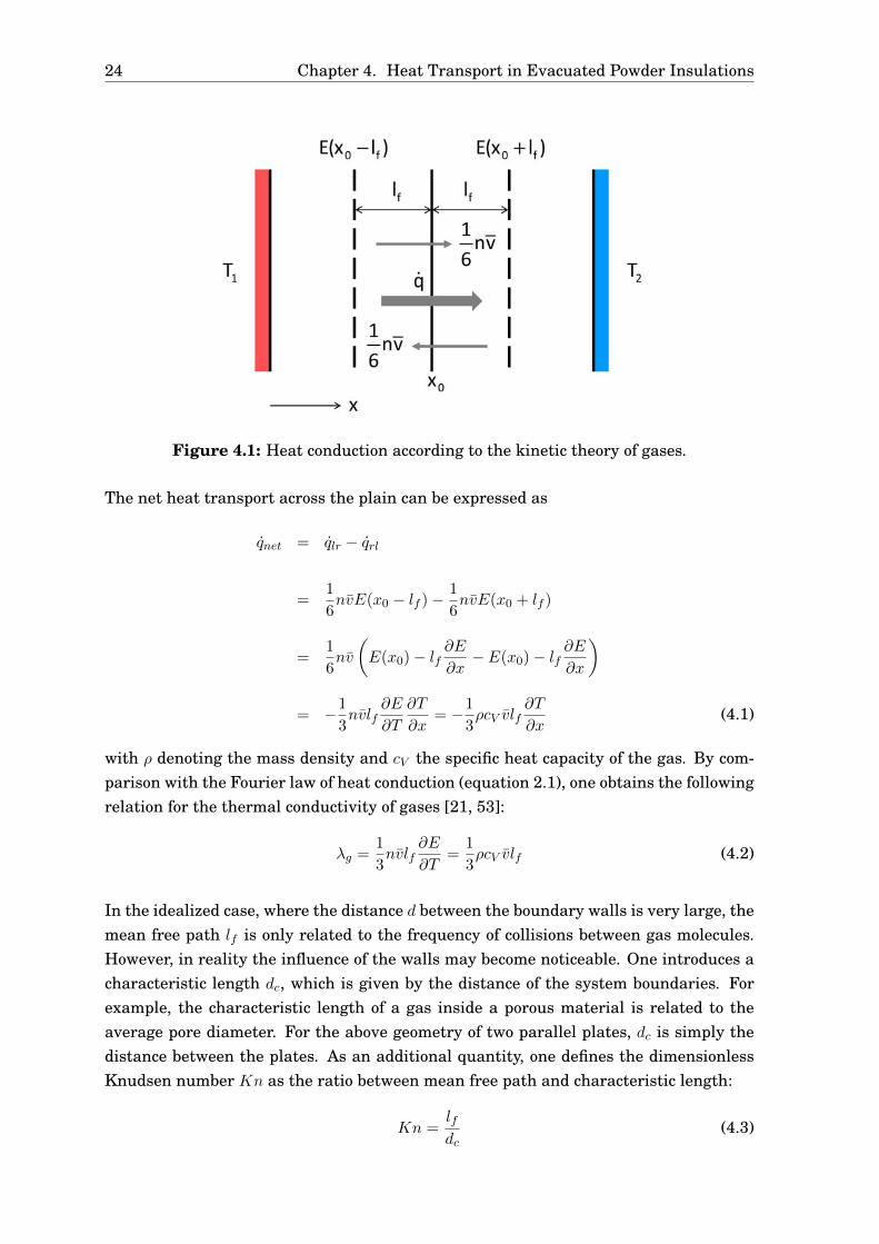
Consider a gas enclosed between two walls of different temperatures and an imaginaryplane at position x0 (figure 4.1). The number of gas molecules per unit time per unit areathat cross the plane in one direction is given by nv/6, where n is the particle density andv is their average velocity according to the Maxwell-Boltzmann distribution. The factor1/6 is due to the fact that particle motion is possible in all three dimensions of spacewith a positive and a negative direction for every dimension. The mean distance whichthe molecules can travel freely between collisions with other particles is called mean freepath lf . Since both the distance between the walls and the gas density are assumed to bevery large, collisions with the boundary walls can be neglected compared to the numberof gas-gas-collisions. The thermal energy E = kBT/2 of the particles is a function oftheir temperature, and as temperature varies along the x-direction, also E depends onx. Molecules crossing the plane from the left have the mean energy Elr = E(x0 − lf ),because their last collision was at an average distance lf from the plain. In analogy,particles from the right carry the average thermal energy Erl = E(x0 + lf ).
24 Chapter 4. Heat Transport in Evacuated Powder Insulations
Figure 4.1: Heat conduction according to the kinetic theory of gases.
The net heat transport across the plain can be expressed as
qnet = qlr − qrl
=1
6nvE(x0 − lf )−
1
6nvE(x0 + lf )
=1
6nv
E(x0)− lf
∂E
∂x− E(x0)− lf
∂E
∂x
= −1
3nvlf
∂E
∂T
∂T
∂x= −1
3ρcV vlf
∂T
∂x(4.1)
with ρ denoting the mass density and cV the specific heat capacity of the gas. By com-parison with the Fourier law of heat conduction (equation 2.1), one obtains the followingrelation for the thermal conductivity of gases [21, 53]:
λg =1
3nvlf
∂E
∂T=
1
3ρcV vlf (4.2)
In the idealized case, where the distance d between the boundary walls is very large, themean free path lf is only related to the frequency of collisions between gas molecules.However, in reality the influence of the walls may become noticeable. One introduces acharacteristic length dc, which is given by the distance of the system boundaries. Forexample, the characteristic length of a gas inside a porous material is related to theaverage pore diameter. For the above geometry of two parallel plates, dc is simply thedistance between the plates. As an additional quantity, one defines the dimensionlessKnudsen number Kn as the ratio between mean free path and characteristic length:
Kn =lf
dc(4.3)
4.1. Gas Heat Conduction and Smoluchowski Effect 25
Expressed by the Knudsen number, three different regimes of gas heat conduction canbe distinguished:
A) Continuum (Kn 1): Collisions with the boundary walls become negligible ifdc lf , which corresponds to Kn 1. This is exactly the previously described case,where the heat conductivity is given by equation 4.2. From the kinetic theory of gases[53], it is known that the mean free path is inversely proportional to the particle (andmass) density: lf ∼ n
−1 ∼ ρ−1. The expression for λg contains the product ρlf and
the quantities cV and v, which do not depend on pressure for an ideal gas. As a firstimportant result, it follows that the thermal conductivity is independent of gas pressure.The heat transport for Kn 1 is also referred to as heat diffusion, because it is onlyrelated to collisions of gas molecules along their random walk.
B) Free Molecular Flow / Knudsen Flow (Kn 1): In the opposite case with dc lf ,which for example occurs at low gas pressures or small pore diameters, the collisions be-tween the molecules can be neglected. Thus, thermal energy is directly transferred be-tween the boundary walls. This situation is also called ballistic transport. Equation 4.2is still valid, but lf has to be replaced by dc, which is the new effective distance thatparticles can travel before they hit the walls. Because dc is a constant, but the term forλg still includes the density ρ, which is proportional to the gas pressure, the thermalconductivity becomes a linear function of pressure. In a perfect vacuum, λg approacheszero, and gaseous conduction is suppressed.
C) Transition Regime (Kn ≈ 1): Whereas the limiting cases above could be treatedstraight-foreward, the discussion of gas heat conduction in the transition range betweencontinuum and free molecular flow becomes rather complicated. In a detailed investi-gation of gas conduction in evacuated solar thermal collectors, different calculation ap-proaches have been collected and discussed [35]. The most general method is solvingthe Boltzmann transport equation [54], which is connected to a considerable calcula-tory effort. Analytical solutions are only known for simple geometries and within nar-row pressure and temperature intervals. Another possibility is the temperature-jumpmethod, which assumes Fourier’s law to be valid also in the transition regime, but atthe same time uses different boundary conditions at the walls. In its original form, thismethod was applicable only in the region of Kn < 0.1 [55]. A modified version of thetemperature-jump method has been developed, which is valid for a significantly largerrange of Knudsen numbers, but requires the solution of the heat equation with mixedboundary conditions [35]. Finally, a simple and heuristic equation derived from exper-imental data is known, which interpolates the thermal conductivity in the transitionregime [34, 56]:
λg =λ0
1 + 2βSKn=
λ0
1 +p1/2p
(4.4)
Here, λ0 is the heat conductivity in the continuum, and p1/2 is the characteristic pres-sure at which λg reaches half of the continuum value. βS is an experimentally deter-mined constant. For air, the values are p1/2 = 230mbar/ (dc [µm]) and βS = 1.6 [57].
26 Chapter 4. Heat Transport in Evacuated Powder Insulations
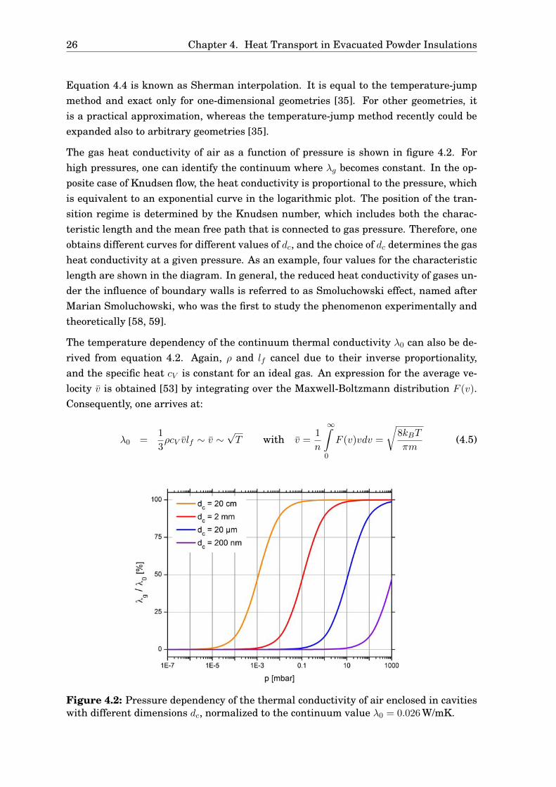
Equation 4.4 is known as Sherman interpolation. It is equal to the temperature-jumpmethod and exact only for one-dimensional geometries [35]. For other geometries, itis a practical approximation, whereas the temperature-jump method recently could beexpanded also to arbitrary geometries [35].
The gas heat conductivity of air as a function of pressure is shown in figure 4.2. Forhigh pressures, one can identify the continuum where λg becomes constant. In the op-posite case of Knudsen flow, the heat conductivity is proportional to the pressure, whichis equivalent to an exponential curve in the logarithmic plot. The position of the tran-sition regime is determined by the Knudsen number, which includes both the charac-teristic length and the mean free path that is connected to gas pressure. Therefore, oneobtains different curves for different values of dc, and the choice of dc determines the gasheat conductivity at a given pressure. As an example, four values for the characteristiclength are shown in the diagram. In general, the reduced heat conductivity of gases un-der the influence of boundary walls is referred to as Smoluchowski effect, named afterMarian Smoluchowski, who was the first to study the phenomenon experimentally andtheoretically [58, 59].
The temperature dependency of the continuum thermal conductivity λ0 can also be de-rived from equation 4.2. Again, ρ and lf cancel due to their inverse proportionality,and the specific heat cV is constant for an ideal gas. An expression for the average ve-locity v is obtained [53] by integrating over the Maxwell-Boltzmann distribution F (v).Consequently, one arrives at:
λ0 =1
3ρcV vlf ∼ v ∼
√T with v =
1
n
∞
0
F (v)vdv =
8kBT
πm(4.5)
Figure 4.2: Pressure dependency of the thermal conductivity of air enclosed in cavitieswith different dimensions dc, normalized to the continuum value λ0 = 0.026W/mK.

4.1. Gas Heat Conduction and Smoluchowski Effect 27
One could have also obtained the relation v ∼√T from E = 1
2kBT = 12mv2. However,
this derivation is somewhat sloppy, because the mean square speed v2 has to be distin-guished from the squared average speed v
2 is ignored. Actually, v2 and v2 differ from
each other only by a constant factor of 8/3π, which does not matter for the temperature-dependency. But this fact can only be derived from integrating both v and v
2 over theMaxwell-Boltzmann distribution. Therefore, the integral has to be calculated anyway.
Up to now, general properties of the thermal conductivity of gases and their dependen-cies on pressure and temperature have been discussed. In the following, some morespecific aspects are presented, which may become relevant under practical conditions.First of all, an important relation is obtained from a closer look at the different quanti-ties that determine the heat conductivity of a gas according to equation 4.2:
λg =1
3ρcV vlf ∼ f
ς√M
(4.6)
with ρ ∼ M cV ∼ f
Mv ∼ 1√
Mlf ∼ 1
ς
As a consequence, gases with a high cross section ς for collisions, a high molar mass M
and few degrees of freedom f have lower thermal conductivities. All three requirementsare fulfilled for the inert gases argon, krypton and xenon. These gases consist of onlyone atom. Therefore, degrees of freedom due to rotation and oscillation are not existent,and only the three degrees of freedom connected to translational motion are available.In addition, the atoms are relatively heavy and have a large effective diameter, whichis especially valid for krypton and even more for xenon. The resulting low continuumheat conductivities and other relevant properties of these gases are listed in table 4.1.For comparison, the values for air have also been included.
Air Argon Krypton Xenon
M [g/mol] 14.007 39.948 83.798 131.293
rW [pm] 155 188 202 216
f [1] 6 3 3 3
λ0 [10−3 W/mK] at T = 25 °C 26.1 17.7 9.5 5.6
αHGS 0.83 1 0.5 0.55
αAl 0.95 0.34 0.5 0.4
Table 4.1: Selected properties of argon, krypton and xenon compared to air: molarmass M , van der Waals radius rW , number of degrees of freedom f , continuum heatconductivity λ0 and accommodation coefficients α for high-grade steel and aluminum.For air, the values of M , rW and f refer to pure nitrogen [34, 35, 44, 66, 67, 68, 69].

28 Chapter 4. Heat Transport in Evacuated Powder Insulations
From a more detailed investigation [35] based on the temperature-jump method accord-ing to [55] and [58], one can derive equation 4.7, which describes the gas heat conductiv-ity in a very explicit way. It contains the pressure dependency according to equation 4.4,the temperature dependency from equation 4.5 and also includes the parameters f , ςand M from equation 4.6:
λg (p, T ) =
RT8πM
16√2ς
5πkB(2f+9) +T
pdcαred(f+1)
(4.7)
In addition to the already defined quantities, the gas constant R = 8.31J/K mol andthe reduced accommodation coefficient αred, which shall be explained later, occur in thisterm. For the limiting case of p → ∞, which corresponds to the continuum, one canneglect the second summand in the denominator to obtain equation 4.8, which is a moreprecise version of equation 4.6:
λg ∼ (2f + 9)√T
ς√M
(4.8)
In the opposite situation where p → 0, the first addend can be ignored, which yields:
λg ∼ pαred (f + 1)√MT
(4.9)
In this case of ballistic heat transport, the interactions between molecules can be ne-glected compared to collisions with the boundary walls (see page 25). It is thereforecomprehensible that the cross section ς for intermolecular collisions does no longer mat-ter. Instead, an accommodation coefficient α occurs, which describes the interactionwith the walls. It is defined as:
α =Tout − Tin
Twall − Tin(4.10)
If the incoming particles with temperature Tin adopt the wall temperature completely,which means Tout = Twall after the collision, the accommodation coefficient is α = 1. Thesituation where there is no temperature exchange at all (Tout = Tin) is described by anaccommodation coefficient of α = 0. The intermediate cases are expressed by 0 < α < 1,according to how big the temperature change is. The coefficients for a specific gas varyfor different wall materials. As an example, the values for nitrogen, argon, krypton andxenon in combination with high-grade steel and aluminum are listen in table 4.1.
For the usual case where a gas is enclosed between two parallel plates with accommo-dation coefficients α1 and α2, the reduced accommodation coefficient has to be used toinclude the interaction with both walls:
αred =α1α2
α1 + α2 − α1α2(4.11)

4.1. Gas Heat Conduction and Smoluchowski Effect 29
If the surface areas of the boundary walls are not equal, for example in cylindrical ge-ometries, the reduced accommodation coefficient in equation 4.9 has to be replaced bythe area-asymmetric accommodation factor f (αi, Ai) to correct the errors of the stan-dard temperature-jump method at low gas pressures. An expression for f (αi, Ai) wasfirst derived by [70]:
f (αi, Ai) =
1
A1α1+
1
A2
1
α2− 1
−1
(4.12)
Putting everything together, the thermal conductivity of the inert gases argon, kryptonand xenon is lower compared to nitrogen not only in the continuum, but also in theregime of free molecular flow due to beneficial accommodation coefficients, a high mo-lar mass and a low number of degrees of freedom. This fact has also been confirmedexperimentally [35]. On a sidenote, this does not automatically have to be true. For ex-ample, sulfur hexafluoride SF6 has a lower heat conductivity than nitrogen in the con-tinuum because of its high mass and large diameter. However, in the Knudsen regime,its thermal conductivity is higher. This is a result of disadvantageous accommodationcoefficients and the high number of degrees of freedom (fSF6 = 19), which are weighteddifferently in the regime of free molecular flow (factor 2f + 9 versus f + 1, see equa-tions 4.8 and 4.9).
In practical applications with evacuated powder insulations, it may be reasonable toreplace air with an inert gas, for example if the vacuum pressure that is necessary fora complete suppression of gaseous conduction cannot be maintained because of tech-nically unavoidable leakages. In this case, the insulating properties of inert gases de-scribed above can be utilized. In real applications, due to the entrance of air through theleakage, a gas mixture will be present though, and the fraction of air will increase withtime. It is known [71] that the thermal conductivity of gas mixtures can be expressedby the following formula if the pressure is in the continuum regime for both gases:
λtot =λ1p1 + λ2p2
p1 + p2=
λ1p1P2
+ λ2p1p2
+ 1(4.13)
λi and pi are the continuum heat conductivities and the partial pressures of the singlecomponents. The combined thermal conductivity λtot only depends on the ratio of partialpressures. In a logarithmic plot, one obtains an S-shaped curve, which is shown infig. 4.3 for a mixture of air and krypton.
Although the thermal conductivity of inert gases is well-known, the effective heat con-ductivity of an evacuated perlite powder insulation under the influence of argon andkrypton has been measured in the experimental part of this thesis (section 6.3). Themain motivation of these measurements was to verify the demonstrated effects for per-lite and to investigate the coupling effect for inert gases.

30 Chapter 4. Heat Transport in Evacuated Powder Insulations
Figure 4.3: Total thermal conductivity of a gas mixture of air and krypton in the con-tinuum at T = 25 °C as a function of partial pressure ratio [71].
4.2 Solid Heat Conduction
As mentioned in section 2.1, conductive heat transfer in solids can be due to phonons orelectrons. However, the electronic heat transport requires mobility of electrons, whichis only given in metals and, to a lower extent, in semiconductors. Heat insulation mate-rials are usually not electrically conducting, since the electrons are bound to the latticeatoms. Therefore, only the phononic heat transport occurs. For porous materials, tworelevant solid heat conductivities can be distinguished. On the one hand, there is theheat conductivity λ
∗s, which describes the massive part of the solid without any effects
that are related to the material structure. On the other hand, there is the effective solidheat conductivity λs, which takes into account the morphology of the material.
For the theoretical characterization of λ∗s, the phononic heat transport has to be consid-
ered. From a physical point of view, one can treat phonons like an ideal gas of particlesconfined in the volume of the solid. As a consequence, the results from kinetic theoryof gases can be transferred, and equation 4.2 is still valid if the values v and lf areadjusted for phonons. The quantity v, which previously was the mean velocity of gasmolecules according to the Maxwell-Boltzmann distribution, has to be replaced by thegroup velocity of phonons, which is obtained from the dispersion relation. Regarding themean free path lf , one has to consider both phonon-phonon-scattering and scattering ondefects and impurities.
In order to describe the temperature dependency of the solid heat conductivity in detail,it has to be taken into account that both the specific heat cV of the solid and the meanfree path lf of phonons can vary with temperature [60]. For the description of cV at

4.2. Solid Heat Conduction 31
low temperatures, a quantum mechanical treatment is necessary. However, at hightemperatures (room temperature), the specific heat capacity approaches the classicallyobtained Dulong-Petit value of cV = 3NkB/m = const. where N is the total number ofatoms and m is the mass of the solid. Therefore, only the mean free path lf determinesthe temperature dependency of the solid heat conductivity λ
∗s. At high temperatures,
scattering on defects can be neglected, and only phonon-phonon scattering is relevant.As a consequence, lf becomes inversely proportional to T [60]:
λ∗s ∼
1
T(4.14)
The effective solid heat conductivity λs of a porous insulation material is usually muchsmaller than λ
∗s [10], because the morphology of these materials influences the heat
transport (see figure 4.4). The heat flux (red arrow) can not always be aligned parallelto the temperature gradient and has to follow an indirect route, because the direct path-way is obstructed by the presence of pores. As an additional effect in the case of powders,the transition to an adjacent grain can only happen at the small contact area, which ispointlike in an idealized view . The combination of both effects results in small effectivesolid heat conductivities. In other words, there are additional thermal resistances aris-ing from the structure of the material. A very demonstrative example for these effectsis the highly-porous perlite: The two major components of this material are SiO2 (65to 75 %) and Al2O3 (10 to 15 %) with thermal conductivities of λ∗
SiO2≈ 1.2 W/mK and
λ∗Al2O3
≈ 28 W/mK [44]. Therefore, λ∗perlite is supposed to be in the order of 1 W/mK.
Typical values for λs are 2 to 3 orders of magnitude lower.
It is obvious that the effective solid heat conductivity λs rises with higher bulk densities,because the volume ratio between massive solid and pores increases. From empiricalfindings, the following relation between λs and the bulk density ρ of the material isknown:
λs ∼ ργ (4.15)
The scaling parameter γ can vary between 1 ≤ γ ≤ 2 depending on the type of material[41, 57, 61, 62].
Figure 4.4: Illustration of solid conduction in a porous powder.

32 Chapter 4. Heat Transport in Evacuated Powder Insulations
4.3 Radiative Heat Transfer
In section 2.3, the heat exchange between two gray surfaces due to radiation was treated,where the intermediate space between the surfaces was supposed to be evacuated. Asa consequence, there was no attenuation of radiation by absorption or scattering, andthermal energy was directly transferred from one surface to the other (comparable toballistic heat transport for gases in section 4.1).
The situation changes if the radiative heat transfer in an evacuated powder is consid-ered, because a certain amount of radiation will be absorbed by the material. As a firstassumption, one could think that the intensity I of radiation at the position x inside themedium follows the Lambert-Beer law, which describes the attenuation of (especiallyhigh-energetic) radiation as a result of absorption:
Ix = I0 exp (−κx) (4.16)
In this equation, the coefficient κ expresses the ability of the material to absorb radi-ation. However, it has to be said that thermal radiation is not only absorbed by thepowder, but also constantly emitted due to its temperature. Therefore, equation 4.16becomes invalid. As already mentioned in section 3.3.2, the emission is distributed ho-mogeneously into all spatial directions. Furthermore, scattering of radiation occurs.It is therefore necessary to apply the heat diffusion model to infrared-photons. Onceagain, one can proceed like in section 4.1 to obtain an expression for the radiative heattransport (compare to equation 4.1):
qnet = −1
3nvlf
∂E
∂T
∂T
∂x(4.17)
Now some specifications have to be made to represent a gas of photons, which are theparticles related to the exchange of electromagnetic radiation. At first, the productn (∂E/∂T ) is equivalent to the temperature derivative of the energy density u which canbe obtained from Planck’s law:
u(T ) =
∞
0
u(ν, T )dν =
∞
0
8πhν3
c3
1
exp
hνkBT
− 1
dν
=8πn3
k4BT
4
h3c3
∞
0
x3
exp(x)− 1dx
=8πn3
k4BT
4
h3c3
π4
15=
4σn3T4
c
n∂E
∂T=
∂u
∂T=
16σn3T3
c(4.18)

4.3. Radiative Heat Transfer 33
For this derivation, the spectral energy density u(ν, T ) as a function of frequency ν hasbeen used. The refractive index n = c/c has been introduced, where c is the propa-gation velocity of radiation inside the medium. For the evaluation of the integral, thesubstitution x = hν/kBT has been applied. The occurring constants have been com-bined using the Stefan-Boltzmann constant σ. The result for ∂u/∂T can be inserted intoequation 4.17. With v = c and by expressing the mean free path lf of phonons as thereciprocal of an extinction coefficient Eex(T ) (see equations 4.22 to 4.28), one arrives at[10]:
qnet = −1
3
c
n
1
Eex(T )
16σn3T3
c
∂T
∂x=
16σn2T3
3Eex(T )
∂T
∂x(4.19)
In the case of diffusive radiation propagation, it is now reasonable to introduce a radia-tive heat conductivity λr by comparing equation 4.19 with Fourier’s law (equation 2.1)to obtain [57]:
λr =16σn2
T3r
3Eex(Tr)(4.20)
Here, Tr denotes the so-called radiation temperature, which is a mean value of theboundary temperatures T1 and T2 defined as:
T41 − T
42 = 4T 3
r (T1 − T2) ⇒ Tr =3
1
4
T21 + T
22
(T1 + T2) (4.21)
For small temperature differences and planar geometries, Tr approaches the arithmeticmean temperature Tr =
12 (T1 + T2).
In the following, the extinction coefficient Eex(Tr) is described more explicitly. First,a spectral mass-specific extinction coefficient e
∗λ(λ) is defined. As already mentioned
above, both scattering and absorption contribute to the extinction of thermal radiationin a given material. Both mechanisms are wavelength-dependent in general. The spec-tral mass-specific extinction coefficient e
∗λ(λ) is then obtained by adding the spectral
mass-specific scattering coefficient s∗λ(λ) and the spectral mass-specific absorption coef-ficient a∗λ(λ) [63]:
e∗λ(λ) = s
∗λ(λ) + a
∗λ(λ) (4.22)
The quantity e∗λ(λ) can be interpreted as the fraction Ie(x,λ)/I0 of radiation that is
scattered or absorbed on its way through a thin layer of matter, divided by the massdensity ρ and the layer thickness x:
e∗λ(λ) =
Ie(x,λ)
I0ρx(4.23)

34 Chapter 4. Heat Transport in Evacuated Powder Insulations
The normalization is reasonable, since the extinction will generally increase for highervalues of ρ and x. Therefore, e∗λ(λ) is a material constant. The ratio Ie(x,λ)/I0 can beexpressed by the layer thickness x and the mean free path lf (λ) of photons:
Ie(x,λ)
I0=
x
lf (λ)(4.24)
This becomes obvious by considering some special cases: If x = 0, which is equivalentto the absence of a medium, radiation will not be extinguished at all, thus Ie(0,λ) = 0.For increasing values of x, the absorbed or scattered fraction will rise proportionally. Ifx = lf (λ), every incoming photon gets scattered or absorbed exactly once, and thereforethe relation Ie(lf ,λ)/I0 = 1 is valid. For x > lf (λ), multiple scattering or absorptionand re-emission occurs, which is expressed by Ie(lf ,λ)/I0 > 1. By inserting the relationIe(lf ,λ)/I0 = 1 into equation 4.23, one obtains an important correlation between themass-specific extinction coefficient and the mean free path:
e∗λ(λ) =
1
ρlf (λ)⇔ lf (λ) =
1
ρe∗λ(λ)
(4.25)
Up to now, all quantities have been functions of wavelength. In order to eliminate thisdependency and to obtain average values, one has to integrate over the whole wave-length spectrum [63]:
1
e∗(T )=
´∞0
1e∗λ(λ)
fR(λ, T )dλ´∞0 fR(λ, T )dλ
(4.26)
with fR(λ, T ) =∂IB(λ, T )
∂IB(T )(4.27)
Different wavelengths are weighted using the Rosseland function fR(λ, T ), which is de-fined as the partial derivative of the spectral blackbody intensity IB(λ, T ) at a giventemperature with respect to the total intensity IB(T ) irradiated at the same temper-ature. Therefore, the Rosseland weighting function favors wavelengths according totheir fraction of occurrence within the blackbody spectrum. As a consequence, the to-tal mass-specific extinction coefficient e
∗(Tr) receives a weak temperature-dependence.This is related to the wavelength shift of the Planck spectrum with varying temperature(compare to Wien’s displacement law, equation 2.14).
Finally, by multiplying the total mass-specific extinction coefficient e∗(Tr) with the den-sity ρ, one arrives at the initially introduced extinction coefficient Eex(Tr). It is thereciprocal of the effective mean free path lf,eff , which is averaged over all wavelengths[57]:
Eex(Tr) = ρe∗(Tr) =
1
lf,eff(4.28)
4.3. Radiative Heat Transfer 35
The extinction coefficient Eex(Tr) is needed to calculate the radiative heat conductivityλr (see equation 4.20). Eex(Tr) is no longer a material constant, but a characteristicproperty of a given material sample with density ρ. In this context, it has to be notedthat the bulk density of powders can vary considerably between different samples. Fur-thermore, the material can be compressed by external forces, by its own weight or byvibrations which cause the grains to align in a more compact packing of spheres.
By means of the previous result, one can deduce a criterion that indicates whether theheat diffusion model is suitable for a given case or not. From the requirement thatthe mean free path lf,eff has to be much smaller than the thickness d of the materialsample, one obtains with equation 4.28:
lf,eff d ⇒ 1
ρe∗(Tr) d ⇒ dρe
∗(Tr) 1 (4.29)
A given sample between two surfaces at temperatures T1 and T2 is called optically thickif dρe
∗(Tr) 1. In this case, the heat diffusion model can be applied, and the totalheat exchange no longer depends on surface emissivities [10]. To reduce the heat flux,one has to maximize the optical thickness τ0 = dρe
∗(Tr). The extinction e∗(Tr) depends
mainly on optical properties of the material, especially on the effective cross section forscattering and absorption. For example, a practical method to increase e
∗(Tr) is theintroduction of highly absorbing soot particles.
As a final note, it is remarkable from a physical point of view that all three mechanismsof gas heat conduction, solid heat conduction and radiative heat transfer can be de-scribed in an analog way by assuming a gas of particles (accordingly molecules, phononsor photons) and using the kinetic theory of gases. This procedure is very fundamentalfor the physical description of heat transport. For example, it is also possible to derivean expression for the heat conductivity of metals if one considers a free electron gas andadjusts equation 4.2 respectively [60].

36 Chapter 4. Heat Transport in Evacuated Powder Insulations
4.4 Coupling Effect
As pointed out in section 4.2, powders have small effective solid thermal conductivities,which is mainly due to thermal resistances as a consequence of pointlike contacts be-tween the grains. However, when the intermediate space between the grains is filled bya gas, the thermal resistances are shorted by gaseous conduction [41, 42, 57, 61]. There-fore, an additional mode of heat transfer occurs, which is referred to as coupling effectand quantitatively expressed by the coupling heat conductivity λc. Conduction via thegas inside the pores remains unaffected. The coupling effect can be significant at moder-ate vacuum pressures (p > 10mbar) and at ambient pressure. Values of λc = 0.02W/mKup to λc = 0.03W/mK are possible for powders [41, 57], which is in the range of thecontinuum heat conductivity of air. In order to suppress the coupling, the material hasto be sufficiently far evacuated, typically below 1 mbar.
In this thesis, a special model has been developed with the aim to quantify the couplingeffect for perlite. It starts out from an existing model for particle beds in general [64],which has been adapted also for aerogels [42]. Although some simplifications are in-troduced, the measured data for perlite can successfully be described (see sections 6.2.2and 6.3.2).
For an illustration of the model, the heat transport between two perlite grains is shownin figure 4.5, both with and without coupling. The particles are supposed to be spher-ical, which is an appropriate assumption for perlite [65]. If the material is completelyevacuated (image a), the situation is exactly like in section 4.2, where the heat flow isrestricted by the pointlike contact between the grains. A possible pathway is indicatedby the red arrow. In the presence of a gas (image b), there are additional routes whichinvolve heat transport along the solid backbone (red arrows) and via the gas (blue ar-rows). At the grain border, a transition between solid and gaseous conduction occurs.As a consequence, the coupling thermal conductivity can be calculated from a serial con-nection of thermal resistances, which are defined in analogy to electrical resistances andfollow the same rules for serial and parallel connection:
Rel =d
Aσel⇒ Rth =
d
Aλ
Rtot =N
i=1
Ri for serial connection
1
Rtot=
N
i=1
1
Rifor parallel connection (4.30)
In the above definition, σel is the electrical conductivity, d is the length of the conductorand A is the reference area.

4.4. Coupling Effect 37
Applying these relations to the serial connection of solid and gaseous conduction de-scribed above, one arrives at:
λc = (1−Π)
1− Γ
λ∗s
+ Γ
λ0
1 +pc1/2p
−1
−1
(4.31)
It is assumed that the thermal conductivity for the heat transport along the massivesolid backbone is equal to λ
∗s (see section 4.2). For the gas heat conduction, the ex-
pression from equation 4.4 is inserted. λ0 is the continuum thermal conductivity of thegas, and p
c1/2 is the characteristic pressure. Because the effective gap size between the
grains is different from the average pore diameter, the characteristic pressures pc1/2 for
coupling and pg1/2 for gaseous conduction inside the pores are expected to vary from each
other. The solid and gaseous contributions to the coupling effect are weighted by thefactor Γ, which is related to the relevant pathlengths of the solid and gaseous phase andwill be explained below. The overall term is weighted by 1 − Π, where Π is a modifiedporosity which only takes into account the volume of the pores [42]. It differs from theconventional porosity Ψ which also includes the volume of the empty space between thegrains. As a consequence, the weighting factor 1 − Π is equal to the volume fraction inwhich coupling occurs.
Due to the fact that the heat conductivity λ∗s along the solid is in the order of 1 W/mK
(see section 4.2) and thus much larger than the maximum heat conductivity of the gas(λ0 = 0.026W/mK for air at T = 25 °C), the first addend in equation 4.31 is expected tobecome negligible in practice. As an approximation, the coupling thermal conductivitycan consequently also be written as:
λc =1−Π
Γ
λ0
1 +pc1/2p
= Φλ0
1 +pc1/2p
(4.32)
Here, the factors 1−Π and 1/Γ have been summarized to a general weighting factor Φ.
Figure 4.5: Coupling effect for a powder consisting of spherical particles. Gas heatconduction inside the pores is not depicted.

38 Chapter 4. Heat Transport in Evacuated Powder Insulations
In the following, the weighting factor Γ is described in more detail: Consider the heatflux due to the coupling effect Qc, which flows from the warm end of a perlite sample(thickness Dtot) to the cold end (temperatures T1 and T2). The pathway is composed ofsmall distances di, which are located either in the solid phase (ds,i, depicted red) or in thegas phase (dg,i, depicted blue). On the one hand, the total effective thermal resistanceof the sample due to coupling is given by:
Rth =Dtot
Aλc(4.33)
On the other hand, from the law of serial connections of resistances (equation 4.30), asecond equation for Rth is obtained:
Rth =N
i=1
Ri =N
i=1
di
Aλi=
Ds
Aλ∗s+
Dg
Aλg(4.34)
Here, Ds =
ds,i and Dg =
dg,i are the total distances which the heat flux travels ineither the solid or the gas phase on its way through the perlite sample. λ∗
s and λg are therespective thermal conductivities. By comparing equations 4.33 and 4.34, one arrivesat:
λc =
Ds
Dtotλ∗s+
Dg
Dtotλg
−1
(4.35)
Because Ds +Dg = Dtot, the weighting factor Γ is defined according to:
Dg
Dtot= Γ ⇔ Ds
Dtot= 1− Γ (4.36)
As a consequence, Γ is always smaller than 1. In the simplified coupling model (equa-tion 4.32), the prefactor (1−Π) is also in the range 0 < (1−Π) < 1. Hence, the weight-ing factor Φ = (1−Π) /Γ, which is determined by fitting of experimental data in thisthesis, can theoretically have values between zero and infinity.
Figure 4.6: Thermal resistance model for the coupling effect.
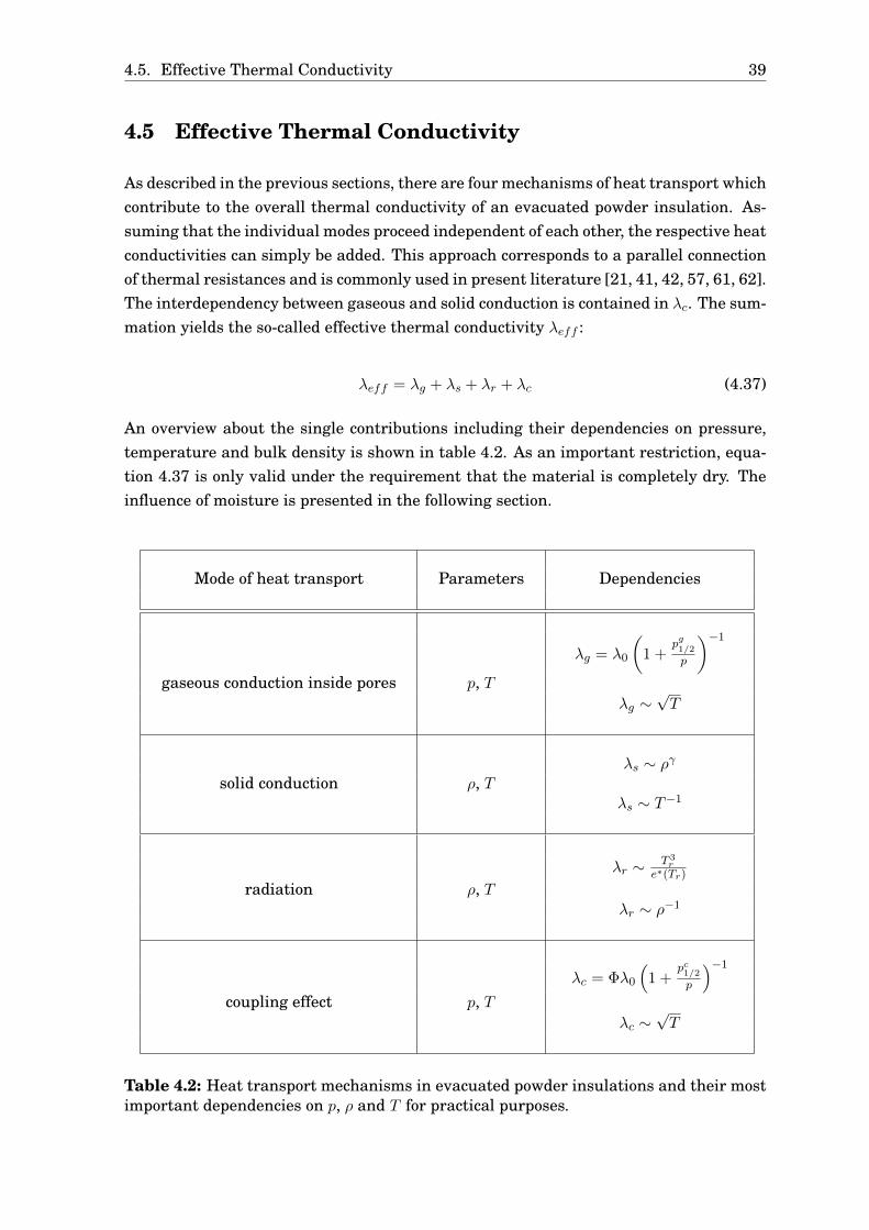
4.5. Effective Thermal Conductivity 39
4.5 Effective Thermal Conductivity
As described in the previous sections, there are four mechanisms of heat transport whichcontribute to the overall thermal conductivity of an evacuated powder insulation. As-suming that the individual modes proceed independent of each other, the respective heatconductivities can simply be added. This approach corresponds to a parallel connectionof thermal resistances and is commonly used in present literature [21, 41, 42, 57, 61, 62].The interdependency between gaseous and solid conduction is contained in λc. The sum-mation yields the so-called effective thermal conductivity λeff :
λeff = λg + λs + λr + λc (4.37)
An overview about the single contributions including their dependencies on pressure,temperature and bulk density is shown in table 4.2. As an important restriction, equa-tion 4.37 is only valid under the requirement that the material is completely dry. Theinfluence of moisture is presented in the following section.
Mode of heat transport Parameters Dependencies
λg = λ0
1 +
pg1/2p
−1
gaseous conduction inside pores p, Tλg ∼
√T
λs ∼ ργ
solid conduction ρ, Tλs ∼ T
−1
λr ∼ T 3r
e∗(Tr)
radiation ρ, Tλr ∼ ρ
−1
λc = Φλ0
1 +
pc1/2p
−1
coupling effect p, Tλc ∼
√T
Table 4.2: Heat transport mechanisms in evacuated powder insulations and their mostimportant dependencies on p, ρ and T for practical purposes.

40 Chapter 4. Heat Transport in Evacuated Powder Insulations
4.6 Influences of Moisture
The considerations of the previous sections were based on the condition of dry insulationmaterials. When moisture is present, additional effects can occur. First of all, it has tobe mentioned that moisture can exist in a gaseous phase in the form of water vaporand in a liquid phase as water. It is obvious that water vapor increases both gaseousconduction and the coupling effect. The thermal conductivity in the continuum regimegiven by is λwv = 0.025W/mK at T = 100 °C [34] and has almost the same value as air.Moreover, the characteristic pressure for gas heat conduction according to equation 4.4can be specified for water vapor: p
g1/2 = 120mbar/(dc [µm]) [57]. In the simultaneous
presence of air or other gases, equation 4.13 for gas mixtures can be used. As anotherobvious effect of moisture, conduction inside a porous structure can be enhanced byliquid water. Due to its high thermal conductivity (λw = 0.6W/mK at T = 25 °C [34, 72]),this can have a significant negative impact. However, this effect requires high moisturelevels and therefore only has a minor relevance in practice.
An additional mode of heat transfer occurring in moistened pores is the so-called porediffusion. This term refers to the transport of latent heat as a result of evaporationand subsequent condensation of water molecules. It requires the pore surface to becompletely covered with a thin layer of water [73]. Consider a moistened pore with atemperature gradient (figure 4.7). In equilibrium, evaporation and condensation happenat equal rates over the whole surface. However, the water molecules will preferablyevaporate in the hot domain and, after a diffusion process, condensate in the cold region.Because the molecules can move back to the hot region via the water layer on the poresurface, the latent heat ∆hv connected to the phase change is transported from one endof the pore to the other. To quantify this effect, the pore diffusion thermal conductivityλdiff is introduced.
Figure 4.7: Pore diffusion: Transport of latent heat inside a pore due to moisture underthe effect of a temperature gradient.

4.6. Influences of Moisture 41
In general, λdiff depends on the vapor diffusion coefficient Dv, the specific heat of evap-oration ∆hv and the saturation vapor pressure psat. The exact dependency on thesequantities is not completely consistent, and there are several formulas in literature toexpress λdiff , which differ slightly from each other [74]. For a bulk material, λdiff isalso correlated to the ratio of open and closed pores, because only open pores are well-accessible for moisture. It is also comprehensible that λdiff increases with temperature,since as it is easier to supply the energy needed for the evaporation at higher temper-atures. If T approaches the evaporation temperature of water at atmospheric pressure(Tev = 100 °C), the pore diffusion heat conductivity of a moistened material can be up to10 times larger than the overall effective heat conductivity of the dry material [74, 75].This is connected to the fact that the transport of latent heat is a very effective modeof heat transfer. Under vacuum, lower temperatures are sufficient to cause the porediffusion effect, because the evaporation temperature decreases with lower pressures.
A general model that can be used to describe the heat transport within moistened insu-lation materials was first developed by Krischer [73]. It has been extended to includematerials with both open and closed pores [74]. The model is based on the followingsteps and assumptions:
• Heat transport within the moistened material can occur via the solid backbone,condensed liquid water, water vapor, other gases (e.g. air) and pore diffusion. Thefive different modes have to be weighted differently according to their occurrencewithin the material.
• Solid conduction is described by λs. It has to be weighted by a factor of 1 − Ψ,where Ψ = 1 − ρ/ρs is the porosity of the material. For this definition, the bulkdensity ρ and the solid density ρs were used. Pores can be either open or closed,thus Ψ = Ψop +Ψcl.
• The heat conductivity for closed pores is denoted with λcl. As closed pores areinaccessible for liquid water by definition, λcl only includes conduction via gases(e.g. air, water vapor) and radiation: λcl = λg + λr. The weighting factor is Ψcl.
• A fraction of open pores described by the factor Ψw is completely flooded with liquidwater. The thermal conductivity inside these pores is given by λw = 0.6 W
mK .
• From the remaining part Ψop − Ψw, the percentage 1 − b is dry, which means thatthere is no pore diffusion. It can be treated in analogy to closed pores with theonly difference being the fact that the gas mixture inside these pores also containswater vapor. Therefore, the thermal conductivity is equal to λop = λg+wv + λr.
• The last fraction of open pores is moistened, and therefore pore diffusion occurs.The heat conductivity in these pores is given by λop + λdiff . The weighting factoris b (Ψop −Ψw).

42 Chapter 4. Heat Transport in Evacuated Powder Insulations
• To obtain an overall thermal conductivity, the thermal resistances connected tothese five modes can be aligned either serial or parallel, depending on the geom-etry and structure of the material. For a parallel connection, the five thermalconductivities add up, which corresponds to the maximum total heat conductivity(compare equation 4.30). By using the weighting factors, one obtains:
λparallel = (1−Ψ)λs +Ψwλw + b (Ψop −Ψw) (λop + λdiff ) +
+ (1− b) (Ψop −Ψw)λop +Ψclλcl (4.38)
For a serial connection, which is equivalent to the lowest possible total heat con-ductivity, the reciprocal values of the heat conductivities add up (equation 4.30),and one arrives at:
λserial =
1−Ψ
λs+
Ψw
λw+
b (Ψop −Ψw)
λop + λdiff+
(1− b) (Ψop −Ψw)
λop+
Ψcl
λcl
−1
(4.39)
• In the general case, one combines a serial and a parallel connection and introducesanother weighting factor a, so that the overall effective heat conductivity is givenby:
λeff =
a
λparallel+
1− a
λserial
−1
(4.40)
It is obvious that λeff (a = 0) = λserial and λeff (a = 1) = λparallel. The weightingfactor a can be determined experimentally.
An illustrative sketch of the combination of serial and parallel connection including thedifferent weighting factors is shown in figure 4.8.
Figure 4.8: Extended Krischer model for the calculation of the effective heat conductiv-ity of moistened materials [73, 74].

4.6. Influences of Moisture 43
For various insulation materials like mineral wool, foam glass, polystyrene, polyurethaneand also perlite, the extended Krischer model has successfully been used to describe thetemperature dependency of the effective thermal conductivity under the effect of mois-ture [74, 75]. However, as a restriction, the measurements have only been performed atambient pressure.
From a look at the phase diagram of water (figure 4.9), one can deduce some importantfacts for the practical relevance of the possible moisture-related effects described above:The triple point of water is at p = 6.1mbar and T = 0.01 °C [72]. At lower pressures,water can only exist in the solid or in the gaseous phase. In vacuum super insulations,the pressure is typically at 0.001mbar ≤ p ≤ 1mbar. As a consequence, pore diffusioncannot occur, because it requires a liquid phase. Above T = 0 °C, the only disadvanta-geous effect that can play a role in practice is the additional gas conduction due to watervapor. In order to reduce the moisture content and to minimize this effect, the insulat-ing material can be baked out. The decrease of the water content with time during abaking-out process is examined experimentally in section 6.4.
Figure 4.9: Phase diagram of water [76].

.

45
Chapter 5
Perlite and Vacuum SuperInsulation: State of the Art
As already mentioned in section 3.3.2, a vacuum super insulation can be realized withany kind of porous insulation material. For large storage tanks and applications undervacuum, powders and granules have a practical advantage, as they can be installed bypouring or air-injection. In contrast, the mounting of plates made of e.g. polyurethaneor foam glass is rather complicated. Especially perlite is a commonly used material forvacuum super insulations. Other granular materials like diatomaceous earth (kiesel-guhr), expanded clay or expanded glass granules are also possible, but their practicalrelevance is not as high. In this chapter, the special properties of perlite which have ledto this fact are described, and the most important applications of vacuum super insula-tion are presented. Furthermore, the results of former research on perlite are outlined,and the motivation for the additional experiments performed in this work is motivated.
5.1 General Properties of Perlite
Perlite [77, 78, 79] is a naturally occurring mineral of volcanic origin. The source mate-rial is obsidian (volcanic glass), which is transformed into perlite by hydration. There-fore, perlite has an amorphous structure and a relatively high water content of up to2 %. The raw material is mainly composed of SiO2 (65 - 75 %) and Al2O3 (10 - 15 %) withsmall amounts of K2O, Na2O, Fe2O3, CaO and MgO. It has a mass density of aroundρ = 900...1000 kg/m³. Due to on-going volcanic activity, the worldwide perlite resourcesare constantly regenerated.

46 Chapter 5. Perlite and Vacuum Super Insulation: State of the Art
In a technical expansion process, raw perlite (figure 5.1 a) is heated to temperatures of850 °C up to 1000 °C, which is close to the glass transition temperature of the amorphousmaterial. As a consequence, the material softens, and enclosed water vaporizes creatinga large number of microscopically small pores. After the water has escaped, the porousstructure is cooled under well-defined conditions and regains its mechanical stability.As a result of the whole process, the volume can be increased by a factor of 7 up to 20compared to the raw material, and the bulk density can be tuned between ρ = 30kg/m³and ρ = 240kg/m³. The low density and the correspondingly high porosity (0.75 ≤ Ψ ≤0.97) are two very characteristic properties of expanded perlite (figure 5.1 b), which alsomake the material suitable for vacuum super insulation. As explained in section 4.1(compare equation 4.4), the effective pore size has a large influence on the pressuredependence of the gaseous heat conductivity.
In practice, other beneficial properties of expanded perlite are the low price (around50 C/m³), the high temperature stability (up to 800 °C) and the fact that it is nonburn-able and therefore meets fire protection regulations. Furthermore, the material is onlyweakly hygroscopic, as the fraction of open pores is relatively low [79]. This is an impor-tant factor, because moisture can dramatically increase the thermal conductivity (seesection 4.6). Apart from the applications for vacuum super insulation, which will betreated in the following sections, there are numerous other fields of application. Forinstance, the material is used in building technology for thermal insulation at ambientpressure, for acoustic insulation and for lightweight plasters and mortars. In horticul-ture, soil can be mixed with expanded perlite to reduce compaction and to improve thepermeability to air. As a last example, the beverage industry uses expanded perlite forfiltering purposes in many production processes [77, 78].
Figure 5.1: Raw (a) and technically expanded (b) perlite [80].

5.2. Vacuum Super Insulation in Cryogenic Engineering 47
5.2 Vacuum Super Insulation in Cryogenic Engineering
Vacuum super insulation with perlite has established itself as a practical and cost-effective method for the storage of liquid gases. A storage tank (figure 5.2) consistsof an inner vessel with a volume of typically a few m³. By a suspension device, it is fixedin the outer container. The annular gap between both vessels is filled with perlite andevacuated into the range of fine vacuum (p ≈ 0.01mbar). At this pressure, the effectivethermal conductivity of the insulation is sufficiently low, because gas heat conductionis suppressed and only solid conduction and radiative heat transport remain. Never-theless, a small heat flux occurs, which causes a fraction of the liquid gas to heat upand evaporate. This has a cooling effect, because the heat of evaporation is withdrawnfrom the liquid. As a consequence of these two antagonizing effects, the temperatureof the liquid stays constant. However, the tank pressure increases. As the inner vesselcan only withstand pressures of a few bar, the excessive pressure has to be exhaustedthrough a safety valve if the gas is not extracted for its intended use over a longer timeinterval [81].
In general, this application of an evacuated perlite insulation is very similar to theintended long-term storage of hot water. However, liquid gases are typically stored be-tween 20 K (hydrogen) and 90 K (oxygen), whereas the storage temperature for hotwater can be up to 373 K (100 °C) and higher if the water is pressurized. This makes aconsiderable difference, as the thermal conductivity of evacuated perlite is temperature-dependent (see chapter 4), especially the radiation part which scales with T
3 (see equa-tion 4.20).
Figure 5.2: Schematical design of a cryogenic storage tank.
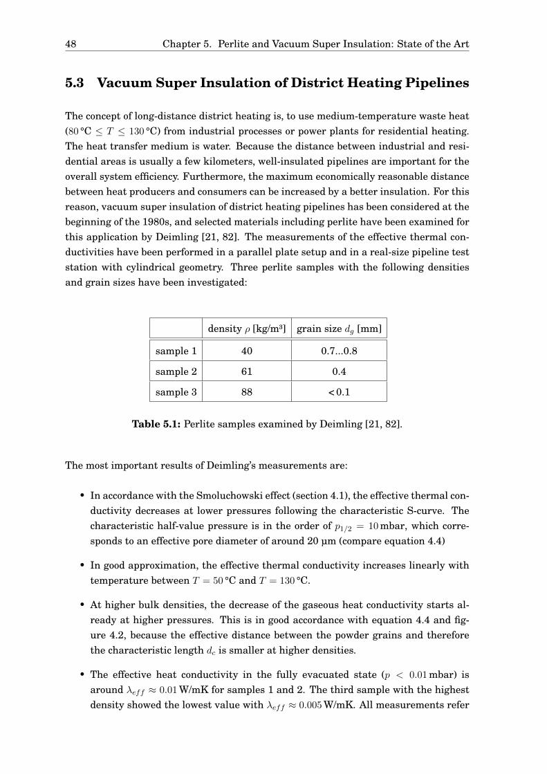
48 Chapter 5. Perlite and Vacuum Super Insulation: State of the Art
5.3 Vacuum Super Insulation of District Heating Pipelines
The concept of long-distance district heating is, to use medium-temperature waste heat(80 °C ≤ T ≤ 130 °C) from industrial processes or power plants for residential heating.The heat transfer medium is water. Because the distance between industrial and resi-dential areas is usually a few kilometers, well-insulated pipelines are important for theoverall system efficiency. Furthermore, the maximum economically reasonable distancebetween heat producers and consumers can be increased by a better insulation. For thisreason, vacuum super insulation of district heating pipelines has been considered at thebeginning of the 1980s, and selected materials including perlite have been examined forthis application by Deimling [21, 82]. The measurements of the effective thermal con-ductivities have been performed in a parallel plate setup and in a real-size pipeline teststation with cylindrical geometry. Three perlite samples with the following densitiesand grain sizes have been investigated:
density ρ [kg/m³] grain size dg [mm]
sample 1 40 0.7...0.8
sample 2 61 0.4
sample 3 88 < 0.1
Table 5.1: Perlite samples examined by Deimling [21, 82].
The most important results of Deimling’s measurements are:
• In accordance with the Smoluchowski effect (section 4.1), the effective thermal con-ductivity decreases at lower pressures following the characteristic S-curve. Thecharacteristic half-value pressure is in the order of p1/2 = 10mbar, which corre-sponds to an effective pore diameter of around 20 µm (compare equation 4.4)
• In good approximation, the effective thermal conductivity increases linearly withtemperature between T = 50 °C and T = 130 °C.
• At higher bulk densities, the decrease of the gaseous heat conductivity starts al-ready at higher pressures. This is in good accordance with equation 4.4 and fig-ure 4.2, because the effective distance between the powder grains and thereforethe characteristic length dc is smaller at higher densities.
• The effective heat conductivity in the fully evacuated state (p < 0.01mbar) isaround λeff ≈ 0.01W/mK for samples 1 and 2. The third sample with the highestdensity showed the lowest value with λeff ≈ 0.005W/mK. All measurements refer

5.4. Vacuum-Super-Insulated Panels in Civil Engineering 49
to a mean sample temperature of T = 75 °C. As a possible explanation, one couldstate that there is a considerable amount of radiative heat exchange, which getsreduced at higher density (compare section 4.3). Obviously, the contribution ofsolid conduction, which increases with density, has only a minor impact. This wasalso a result of the computational evaluation method used by Deimling, where theobtained values of λs were close to zero. Solid conduction was therefore ignored inhis model.
• In general, sample 3 yields the best results regarding the decrease of λeff withpressure (p1/2 ≈ 20mbar) and regarding the value of λeff in the fully evacuatedstate. The sample was prepared by sifting out a very fine fraction with a graindiameter of d < 0.1mm from the original perlite material. The resulting highdensity and the small distance between the powder grains has a beneficial effecton the suppression of radiation and gas heat conduction.
5.4 Vacuum-Super-Insulated Panels in Civil Engineering
As the most recent important application of the vacuum super insulation technology,the so-called vacuum insulation panels (VIP) can be mentioned [83, 84, 85]. This termrefers to insulating plates which have originally been developed for refrigerators. Byintense research and development at ZAE BAYERN during the last decade [57, 61], VIPshave been adapted for the thermal insulation of buildings and are now available on themarket as commercial products. Essentially, a VIP consists of a compressed, evacuatedkernel material, which has to withstand the mechanical load caused by the atmosphericpressure (10 t/m²), and a vacuum-tight laminate (figure 5.3). In the evacuated state, thepanels have an effective thermal conductivity of around λ = 0.007W/mK.
Figure 5.3: Sliced vacuum insulation panel [86].

50 Chapter 5. Perlite and Vacuum Super Insulation: State of the Art
The sealing foil consists of several resilient polymer layers. Since polymers are ratherpermeable for water vapor, nitrogen and oxygen, the foils are coated with a thin alu-minum layer (d = 100nm). The kernel material is usually not perlite, and fumed silicais used instead. This material has a notably finer pore structure with average pore diam-eters of only 200 nm. Therefore, gas heat conduction is already suppressed at relativelyhigh vacuum pressures of 20 to 50 mbar. This is important for the long-term stability ofVIPs. At the beginning of their life cycle, the panels are evacuated to p = 0.1mbar. Witha pressure increase of 1 to 2 mbar per year due to leakages, they maintain their insulat-ing properties over a few decades, and the effective thermal conductivity is expected toremain below λ = 0.008W/mK even after a duration of 50 years [57]. As another benefi-cial consequence of the small pore diameter, the thermal conductivity of fumed silica atambient pressure is only λ = 0.018W/mK [83]. Hence, even when the sealing laminateis damaged and the vacuum inside the panel is destroyed, an effective thermal insula-tion is still existent. To suppress radiative heat transport inside the kernel material,infrared opacifiers like SiC can be introduced.
Compared to conventional insulation materials, the advantage of VIPs is that they reachthe same heat transfer coefficient (k-value) at a much smaller insulation thickness. Toobtain the same k-value as a VIP with a thickness of 5 cm, one would have to use30 cm of conventional insulation. Due to this, VIPs are especially used for insulationapplications under spatial constraints (e.g. due to urban heritage conservation), wherethey are also economically reasonable. The average price of VIPs with a thickness of2 cm is between 50 and 100 C/m².
Apart from building applications, VIPs are also used for cooling of food or pharmaceuti-cals, especially in refrigerated vehicles. Also here, the increase of usable volume pays offthe higher costs of VIPs. To withstand the mechanical stress which occurs for instanceat the bottom of a cooling chamber, the aluminum-polymer laminate can be replaced bythin sheets of high-grade steel.
5.5 Material Selection and Motivation for Additional Re-search
For the vacuum super insulation of the first hot water storage tank prototype (see chap-ter 7), the perlite TECHNOPERL ® - C 1,5 from the Austrian manufacturer EUROPERL,STAUSS PERLITE GMBH is used [79, 87]. This material has already been applied suc-cessfully to liquid gas storage tanks (compare section 5.2). According to the specificationof the manufacturer, the density of an uncompressed bulk is ρ ≈ 53kg/m³, and the grainsize varies between 0 and 1.5 mm. However, it shows in practice that the material canbe compressed up to ρ ≈ 100kg/m³ by vibration or by applying mechanical pressure.Although measurement data for perlite is already known from the work of Deimling(section 5.3), there is still motivation for further investigation of perlite in general and

5.5. Material Selection and Motivation for Additional Research 51
TECHNOPERL ® - C 1,5 in particular:
• The perlite used by Deimling differs from TECHNOPERL ® - C 1,5 regarding grainsize and density, especially sample 3 (see table 5.1), which showed the best results.
• In general, perlite may not always have exactly identical properties, since it is anatural product.
• TECHNOPERL ® - C 1,5 is optimized for cryogenic application and performs wellwithin this temperature range. However, in the temperature regime of hot waterstorage, radiation may have a significantly higher impact. Therefore, it is not clearwhether the existing technology for liquid gas storage can easily be transferredtowards higher temperatures, and whether TECHNOPERL ® - C 1,5 is also theoptimum material for vacuum super insulation of hot water storages.
• The coupling effect in perlite has not been investigated separately by Deimling andis still unclear. Also for other vacuum super insulation materials like aerogels,a fully satisfying agreement between the developed theoretical models and themeasured data has not yet been achieved [42].
• In practice, the utilization of inert gases may help to keep the thermal conductivityconstant for a longer time interval in spite of technically unavoidable leakages ofthe storage tank (see section 4.1). However, the thermal conductivity of perliteunder the influence of these gases has not yet been investigated experimentally.
• Although TECHNOPERL ® - C 1,5 is described to be non-hygroscopic by the manu-facturer [79], it is not known how much moisture (in percent of weight) is actuallycontained.
Because additional research on the material was necessary due to the above reasons,several experiments were performed at ZAE BAYERN (chapter 6). The fundamentaltasks were to quantify the contributions of the different heat transport mechanisms de-scribed in chapter 4 and to investigate the open questions mentioned above. Besides thelaboratory experiments, heat loss measurements on a real-size storage tank prototypewere done in order to study whether the results are also valid under practical conditions(chapter 7).

.

53
Chapter 6
Laboratory MeasurementsRegarding the Heat Conductivityof Evacuated Perlite
The following chapter describes the laboratory experiments which were performed atthe ZAE BAYERN departments in Würzburg and Garching in order to determine thethermal conductivity of TECHNOPERL ® - C 1,5 under various conditions. As a prelimi-nary examination, spectroscopical measurements were done to obtain the radiative heatconductivity (section 6.1). Subsequently, the effective thermal conductivity as a functionof air pressure, bulk density and temperature was measured in a parallel plate setup(section 6.2) for a general understanding of solid and gaseous conduction and the cou-pling effect. Apart from that, effective thermal conductivity measurements were alsoperformed in a cut-off cylinder apparatus (section 6.3) to examine the effects that occur,when argon and krypton are used as filling gases instead of air. This device also servedfor a cross-check of the results from the parallel plate apparatus. Finally, the moisturecontent of TECHNOPERL ® - C 1,5 was determined (section 6.4).
6.1 Spectroscopic Determination of The Radiative Ther-mal Conductivity
If an insulation material is sufficiently far evacuated (p ≤ 10−3 mbar for perlite), gasconduction and coupling are suppressed (λg = λc = 0, see sections 4.1 and 4.4). Inthis state, the total effective thermal conductivity is the sum of radiative and solid heatconductivity:
λeff (p → 0) = λr + λs (6.1)
Because both contributions depend on density and temperature (see sections 4.2 and 4.3),they are difficult to separate by pure thermal conductivity measurements. However,

54 Chapter 6. Laboratory Measurements
there is a different approach to determine the radiative thermal conductivity experi-mentally. As explained in section 4.3, λr is related to the extinction of thermal radiation,which is the combination of scattering and absorption within a material. This propertycan be determined by infrared spectroscopy measurements. The special technique ofFourier transform infrared spectroscopy (FTIR) [88, 89, 90] was used for this purpose.
6.1.1 Principles of FTIR Spectroscopy
The most essential part of an FTIR spectrometer is a Michelson interferometer (fig-ure 6.1). The beam emitted by the IR-radiation source (ideally a blackbody) is collimatedand directed on a semi-transparent mirror, where it is divided into two partial beams.From this point, there are two relevant pathways. The first partial beam is reflected atthe semi-transparent mirror, reflected at the fixed mirror and transmitted on the semi-transparent mirror. The second beam first passes the semi-transparent mirror and isthen reflected both at the moving mirror and at the semi-transparent mirror. At thispoint, the two partial beams are merged, interfere with each other and result in the out-going beam. The outcome of the interference depends on the path difference x, whichcan be calculated from the distances between the mirrors:
x = 2 (dm − df ) (6.2)
For a given wavelength λ, the maximum positive interference occurs if x is an integermultiple of λ. By contrast, if x is an odd-numbered multiple of λ/2, both beams annihi-late each other. Assuming that the intensity of both partial beams is equal (Im = If = I),the intensity Iλ of the outgoing beam due to interference at a single wavelength λ isgiven by:
Iλ = I
1 + cos
2π
λx
= I (1 + cos (2πνx)) (6.3)
Here, the wave number ν = 1/λ = ν/c is introduced, which is defined as the reciprocalof the wavelength. The wave number is proportional to the freqency ν, and the factor ofproportionality is the inverse of the speed of light c. The total intensity of the outgoingbeam as a function of the path difference Itot(x) is then obtained by integrating overall wave numbers in the interval B = [ν1, ν2], which is the so-called bandwidth of thespectrometer:
Itot(x) =
ν2ˆ
ν1
(I(ν) + I(ν) cos (2πνx)) dν (6.4)
The first addend yields a constant which does not contain any relevant information andcan thus be subtracted. This step is usually performed electronically by the spectrome-ter device. Below, only the second addend I(x) is considered:

6.1. Spectroscopic Determination of The Radiative Thermal Conductivity 55
I(x) =
ν2ˆ
ν1
I(ν) cos (2πνx) dν =
∞
−∞
I(ν) cos (2πνx)D(ν)dν (6.5)
By introducing a window function D(ν) which is equal to one for ν ∈ [ν1, ν2] and zerootherwise, the integration boundaries can be extended to plus and minus infinity.
Equation 6.5 already looks similar to a Fourier transform, but the sine term of the trans-formation factor exp(2πiνx) = cos (2πνx) + i sin (2πνx) is missing. However, I(x) is aneven function since I(−x) = I(x), and thus one can replace cos (2πνx) by exp(2πiνx). Theintegral over the sine term must be zero due to the fact that the Fourier representationof an even function may only contain cosine functions which are also even. Therefore,one finally arrives at equation 6.6, which is the definition of the Fourier transform:
I(x) =
∞
−∞
I(ν) exp (2πiνx)D(ν)dν (6.6)
For spectroscopy measurements, one is typically interested in the spectral intensity I(ν).It can be obtained by measuring I(x) and applying the inverse Fourier transform:
I(ν) =
∞
−∞
I(x) exp (−2πiνx)D(ν)dx (6.7)
I (ν) only contains contributions which depend on the path difference x. Constant ad-dends like like thermal irradiation of the investigated sample are filtered out by theFourier transform.
Figure 6.1: Setup of a Michelson interferometer.

56 Chapter 6. Laboratory Measurements
6.1.2 Measurement Procedure
To determine the extinction of thermal radiation, usually three measurements are per-formed:
• A reference measurement (figure 6.2 a), where the outgoing beam of the Michelsoninterferometer is directly detected. An integrating sphere (Ulbricht sphere) is usedto diffuse the beam and to reach a spatially homogeneous intensity.
• A transmission measurement (figure 6.2 b), where the sample is placed in thebeamline, and the transmitted radiation is detected with the aid of the integratingsphere.
• A reflection measurement (figure 6.2 c), where the radiation reflected by the sam-ple is detected.
For all three measurements, the position of the moving mirror is varied, and the result-ing intensities I(x), which are measured at the detector, are recorded. Subsequently,the respective spectral intensities I(ν) are calculated from the inverse Fourier trans-form. The extinction of the sample as a function of the wave number is then given by:
e(ν) =Ireference(ν)− Itransmission(ν)− Ireflection(ν)
Ireference(ν)(6.8)
Figure 6.2: FTIR spectroscopy: Positioning of sample, integrating sphere and detectorfor the reference (a), transmission (b) and reflection (c) measurement.
6.1.3 Experimental Results
For the FTIR spectroscopy measurements of TECHNOPERL ® - C 1,5, thin homogeneouslayers of the perlite powder were prepared on an IR-transparent polymer foil. The mea-sured data for the extinction e(ν) was converted back into units of wavelength. For eachsample, the areal mass density (mass of the sample divided by the area which is cov-ered by the sample) was determined to calculate the mass-specific extinction coefficiente∗λ(λ) (equation 4.23). In figure 6.3, e∗λ(λ) is shown as a function of wavelength. The

6.1. Spectroscopic Determination of The Radiative Thermal Conductivity 57
data of several samples was averaged. The bandwidth of the spectrometer ranged from1.4 to 18 µm and covers the whole wavelength interval which is relevant for thermalradiation at temperatures between approximately 300 and 500 K (compare figure 2.4and equation 2.14).
The remaining procedure to obtain the radiative thermal conductivity is described insection 4.3. First, the total mass-specific extinction coefficient e∗(T ) has to be calculatedusing equation 4.25. As already mentioned, e∗(Tr) has a weak temperature-dependence.A plot of e∗(Tr) versus temperature is shown in figure 6.4 for temperatures between 300and 450 K. In this temperature interval, the total mass-specific extinction coefficientcan be approximated with sufficient accuracy using a second order polynomial (equa-tion 6.9). The error of e∗(Tr) is given by ∆e
∗ = 4m²/kg [63].
e∗(Tr) =
5.32 · 10−4 ·Tr[K]2 − 0.4503 ·Tr[K] + 130.31
m2
kg± 4
m2
kg(6.9)
Eventually, for a given bulk density ρ and radiation temperature Tr (see equation 4.21),the radiative heat conductivity of TECHNOPERL ® - C 1,5 can be calculated from equa-tion 6.10, which follows from equations 4.20 and 4.28:
λr =16σn2
T3r
3ρe∗(Tr)=
16σT 3r
3ρe∗(Tr)(6.10)
For e∗(Tr), the expression from equation 6.9 can be used. The refractive index can be ap-proximated by n = 1. At the temperature regime which is relevant for the conventionalstorage of hot water (T1 = 373 K or lower, T2 = 273 K) and for bulk densities betweenρ = 53kg/m³ and ρ ≈ 100kg/m³ (see section 5.5), one obtains radiative thermal conduc-tivities between λr = 2 · 10−3 W/mK and λr = 5 · 10−3 W/mK (see table 6.1). Comparedto the cryogenic application (T1 = 90 K, T2 = 293 K), the radiative heat conductivity isincreased by a factor of 4 to 5. However, the absolute value of λr still looks promisinglylow, especially at higher densities.
T1 [K] T2 [K] Tr [K] e∗ [m²/kg] ρ [kg/m³] λr [10−3 W/mK]
cryogenic 90 293 208 59.7 53 0.9
application 100 0.5
hot water storage 323 273 299 43.3 53 3.5
low temperature 100 1.9
hot water storage 373 273 326 40.1 53 4.9
high temperature 100 2.6
Table 6.1: Radiative thermal conductivity of TECHNOPERL ® - C 1,5 at different appli-cation temperatures and bulk densities.

58 Chapter 6. Laboratory Measurements
Figure 6.3: Spectral mass-specific extinction coefficient of TECHNOPERL ® - C 1,5 as afunction of wavelength between 1.4 and 18 µm [63].
Figure 6.4: Total mass-specific extinction coefficient of TECHNOPERL ® - C 1,5 asa function of temperature between 300 and 450 K. The error of the measurement is∆e
∗ = 0.004m²/g [63].

6.2. Effective Thermal Conductivity Measurements in a Parallel Plate Setup 59
6.2 Effective Thermal Conductivity Measurements in a Par-allel Plate Setup
After the radiative part of the heat transport had been investigated, the effective ther-mal conductivity of TECHNOPERL ® - C 1,5 was determined experimentally in a parallelplate apparatus at the ZAE BAYERN division in Würzburg. The device [91, 92] has beenespecially developed for thermal conductivity measurements of evacuated super insula-tions and allows the adjustment of vacuum pressure, temperature and bulk density ofthe investigated samples. The variation of these parameters is necessary to examinethe validity of theoretical models and to separate gaseous conduction and the couplingeffect from solid conduction and radiative heat transport.
6.2.1 Measurement Setup and Experimental Procedure
The layout of the parallel plate apparatus is shown in figure 6.5. The central componentsof the device are an electrically heated circular hot plate (2) and two cold plates (3,4)inside a vacuum chamber (1). Two identical samples (5) are placed symmetrically inthe gaps between the metal plates. The inner hot plate has a diameter of dh = 200mmand is surrounded by two guard rings, which are kept at the same temperature Th toprevent radial heat flux. A heat sink (6), which is needed to control the temperature Tc
of the cold plates (dc = 280mm), is realized by circulating a fluid. All temperatures aremeasured using Pt-100 resistances.
Figure 6.5: Layout of the parallel plate apparatus for thermal conductivity measure-ments [91, 92].

60 Chapter 6. Laboratory Measurements
By applying a mechanical force via a piston (9), the density of the investigated samplescan be varied. The sample thickness ds may range from 1 to 28 mm and can be measuredwith an appropriate sensor (10). The heating power Pel, which is needed to keep the tem-perature of the hot plate constant, is regulated by a proportional-integral controller. Itis calculated according to Pel = RelI
2el where Rel is the (temperature-dependent) resis-
tance of the electrical heater and Iel is the current which is measured as the voltagedrop across a 1 Ω precision shunt. In the stationary case, the heating power is equalto the one-dimensional heat flux which flows symmetrically from the hot plate throughboth samples to the cold plates. The assumption of stationary conditions is assumedto be valid when all temperatures and the heating power have remained constant forat least 1.5 hours. The data of the last hour is then averaged to calculate the thermalconductivity of the sample material according to equation 6.11:
λ =Pelds
2A∆T=
2Pelds
πd2h (Th − Tc)
(6.11)
For the evaluation of the measurements, the following systematic errors have to betaken into account [92]:
Temperature: Due to the tolerances of the Pt-100 sensors, the measured temperaturedifference ∆T between hot and cold plates is only accurate within 0.5 K.
Electrical power: Because of the high precision shunt resistance, the relative errorof the heating current is only 0.1 %. However, the resistance of the heater is much lessaccurate. In total, an error of 1 % for the electrical heating power is estimated.
Sample thickness: The absolute error of the thickness sensor is given by 0.2 mm.
Measuring area: The area A = πd2h has a relative error of 0.5 %, which corresponds to
an absolute value of 1.57 · 10−4 m².
Radial heat losses: If the central hot plate and the guard rings are not exactly at thesame temperature, a radial heat flux occurs, which leads to a systematic error. From testmeasurements it is known that the radial heat loss is limited by 0.15 W in the worst casethat can occur in practice. For samples with thermal conductivities above 0.1 W/mK, theheat flux through the sample is typically around 10 W, and thus the relative error dueto radial heat losses is less than 2 %.
For specimens with thermal conductivities smaller than 0.1 W/mK (which is alwaysvalid for super-insulating materials), the heat flux through the sample can become aslow as 0.3 W and is thus in the range of the maximum possible radial heat loss. Forthis case, a special correction method [92] has been developed to avoid high relativeerrors: Based on the assumption that radial heat losses and errors in measured tem-peratures are independent of the temperature difference ∆T between both plates, twomeasurements at different values of ∆T are performed. By taking the difference of bothexperiments, the errors are eliminated:

6.2. Effective Thermal Conductivity Measurements in a Parallel Plate Setup 61
Pel,1 = λ2A
ds∆T1 Pel,2 = λ
2A
ds∆T2
Pel,1 − Pel,2 = λ2A
ds(∆T1 −∆T2)
λ =(Pel,1 − Pel,2) ds2A (∆T1 −∆T2)
(6.12)
In other words, the measurement values are extrapolated to ∆T = ∞, where both therelative error caused by radial heat losses and the relative error of the temperature mea-surement are zero. As a result of the correction method, the remaining error ∆λT+rhl
(not including errors of measuring area, electrical power and sample thickness) is typi-cally around 2 %. According to the law of propagation of uncertainty (equation 6.13), thetotal error of the measurement was calculated according to equation 6.14:
y = y(x1, x2, ..., xn) =⇒ ∆y =n
i=1
∂y
∂xi∆xi
(6.13)
∆λ = ∆λT+rhl +Pelds
2A2∆T∆A+
ds
2A∆T∆Pel +
Pel
2A∆T∆ds =
= λ
2% + 0.5% + 1%+
∆ds
ds
= λ
3.5% +
0.2mmds
(6.14)
For the specific task of measuring the effective thermal conductivity of perlite, two sam-ples of the powder with masses m1 = 76.55 g and m2 = 76.07 g were filled in special clothbags. Before the measurements were started, the samples were baked out at T = 150 °Cand p < 10−3 mbar for a duration of 28 h. When the samples were removed after themeasurements were finished, the masses were m1 = 75.31 g and m2 = 74.69 g. Assumingthat the mass decrease is only due to the evaporation of water which is contained inthe sample, one obtains a moisture content of 1.7 % weight (see section 6.4 for furtherinvestigation regarding moisture content). For the evaluation of the measurements, itis supposed that the samples were completely dry. The temperature differences betweenhot and cold plates for the correction method were ∆T1 = 10K and ∆T2 = 20K.
6.2.2 Presentation and Evaluation of Measurement Results
Because the radiative thermal conductivity has already been determined from the FTIRspectroscopy measurement (see section 6.1.2), the next mode of heat transfer to be in-vestigated is solid conduction. According to equation 6.1, if gaseous conduction andcoupling are suppressed (p < 10−3 mbar), the solid heat conductivity λs at a certain tem-perature T and density ρ can be determined by measuring the total effective thermal

62 Chapter 6. Laboratory Measurements
conductivity and subtracting the radiative thermal conductivity λr, which is calculatedfrom equation 6.10. For this purpose, different measurements were performed in thefully evacuated vacuum chamber at different mean temperatures between 20 °C and150 °C. The sample density was varied by applying an external loading pressure via thepiston. The obtained experimental values for the solid thermal conductivity at differentdensities are depicted in figure 6.6. A linear correlation is observed. From empiricalfindings, λs is expected to scale with ρ
γ (see section 4.2), where γ can have values be-tween 1 and 2. In this case, the linearity corresponds to γ = 1 and is therefore in goodaccordance with theory. In literature, a value close to 1 (1.1 ≤ γ ≤ 1.3) can be found forfumed silica, a material which is quite comparable to perlite [93]. Furthermore, γ ≈ 1
was also determined for polyimide foams [94].
The height of the error bars in figure 6.6 was computed by adding the errors of the effec-tive thermal conductivity measurement (equation 6.14) and the errors of the calculatedvalues for λr, which are mostly caused by the error of the extinction (see equation 6.9).
Different values of λs were measured at equal densities, but different mean tempera-tures. However, no explicit temperature dependency could be observed, although λs ∼T−1 is predicted from theory. A possible explanation is, that this relation is only valid
for crystalline solids. For amorphous materials like SiO2, it has even been observed thatλs slightly rises with temperature [73]. Therefore, the temperature-dependence of λs forperlite, if existing, is assumed to be smaller than the indicated error and neglected fromnow on.
From the linear fit (black line), one obtains the following relation between solid thermalconductivity and density, including standard deviations of the fit parameters:
λs =
(0.326± 0.010) · ρ
kg
m³
− (15.4± 0.7)
· 10−3 W
mK(6.15)
In the next step, effective thermal conductivity measurements at gas pressures between0.1mbar ≤ p ≤ 1000mbar were done in order to examine conduction via the pore gas onthe one hand and the coupling effect on the other hand. A first series of measurementswas recorded at a temperature of T = 20 °C and a bulk density of ρ = 76.3kg/m³. For theevaluation, the pure contribution of gaseous conduction and coupling was determined.For this purpose, the radiation and solid thermal conductivities at the given tempera-ture and density of the sample were calculated according to equations 6.10 and 6.15.Subsequently, the values for λr and λs were subtracted from the measured effectivethermal conductivity λeff to obtain the sum of λg + λc. The result of this procedureis shown in figure 6.7 (blue points), where λg + λc is plotted as a function of pressure.The length of the error bars was calculated by adding the measurement error of λeff
(equation 6.14), the systematic error of λr, which is mainly caused by the extinction e∗,
(equation 6.9) and the statistical error from the linear fit for λs (equation 6.15).

6.2. Effective Thermal Conductivity Measurements in a Parallel Plate Setup 63
Figure 6.6: Solid Thermal Conductivity λs as a function of bulk density, measured in aparallel plate setup.
Figure 6.7: Sum of Gaseous Conduction λs and Coupling Effect λc as a function ofpressure, measured in a parallel plate setup.

64 Chapter 6. Laboratory Measurements
For the interpretation of the experimental data, the well-known relation for gas heatconduction (equation 4.4) and the model for coupling developed in section 4.4 was used.Initially, the more precise version of the coupling model (equation 4.31) was applied:
λg + λc =λ0
1 +pg1/2p
+ (1−Π)
1− Γ
λ∗s
+ Γ
λ0
1 +pc1/2p
−1
−1
(6.16)
The measurement values from figure 6.7 at T = 20 °C were used to fit the parameterspg1/2, Π, Γ λ
∗s and p
c1/2 in equation 6.16 using the software ORIGIN PRO 8.5.1 G. Table 6.2
shows the obtained results and their statistical errors. The quantity λ0 was defined asa constant with λ0 = 25.7 · 10−3 W/mK, which is the continuum thermal conductivityof air at T = 20 °C [34]. It was observed that the outcome of the fitting procedure de-pended on the settings of the initial values. Especially the results for λ
∗s, Π and Γ varied
dramatically, and their errors were unreasonably high in most cases. After testing dif-ferent combinations, a setting of initial values was chosen that resulted in relatively lowerrors. They are also included in table 6.2.
λ0 pg1/2 Π Γ λ
∗s p
c1/2
[10−3 W/mK] [mbar] [1] [1] [10−3 W/mK] [mbar]
value 25.7 5.1 0.87 0.28 35157 39.3
error 0 0.7 1.2 · 106 2.6 · 106 4.5 · 1011 11 · 103
initial value 25.7 5 0.9 0.4 2000 40
Table 6.2: Parameters for gaseous conduction and coupling according to equation 6.16,obtained by fitting the experimental data from figure 6.7 at T = 20 °C.
Still, it has to be said that these results are not very expressive due to the high errors,which are in some cases seven orders of magnitude larger than the indicated values.This is also due to the fact that many parameters were fitted simultaneously, and there-fore the calculation has many degrees of freedom. Especially the value for λ
∗s has a very
large error margin.
Nevertheless, the results from table 6.2 support the assumption from section 4.4 andshow that the term in equation 6.16, which describes the solid contribution to the cou-pling effect, can be neglected. The widely varying value of λ∗
s only proofs that the fittingresults are independent of the choice of λ
∗s. Therefore, the simplified coupling model
according to equation 4.32 was applied:
λg + λc =λ0
1 +pg1/2p
+ Φλ0
1 +pc1/2p
(6.17)

6.2. Effective Thermal Conductivity Measurements in a Parallel Plate Setup 65
This time, the parameters pg1/2, Φ and p
c1/2 were fitted according to equation 6.17. The
results are shown in table 6.3.
λ0 [10−3 W/mK] pg1/2 [mbar] Φ [1] p
c1/2 [mbar]
value 25.7 5.1 0.46 39.3
error 0 0.3 0.02 8.7
initial value 25.7 5 0.4 50
Table 6.3: Parameters for gaseous conduction and coupling according to equation 6.17,obtained by fitting the experimental data from figure 6.7 at T = 20 °C.
It showed that the results of the fitting procedure were largely independent of the se-lection of initial values, and any reasonable combination yielded the same outcome withrelatively small errors. The results for p
g1/2 and p
c1/2 are identical to the values from
table 6.2, and Φ = (1−Π) /Γ = 0.46 from table 6.3 agrees with Π = 0.87 and Γ = 0.28
from table 6.2 (see section 4.4 for the definition of Φ). These facts are considered asfurther indications that the simplified coupling model (equation 4.32) is appropriate todescribe the coupling effect in perlite with sufficient accuracy. As a consequence, thevalues from table 6.3 were used to draw the fitting curve (blue) in figure 6.7 accordingto equation 6.17. The agreement with the measured data is striking.
Considering the results from table 6.3, the following findings can be stated:
• The coupling thermal conductivity in the continuum is λc = (11.8± 0.5) · 10−3 W/mK,which can be calculated from Φ = 0.46± 0.02 and λ0 = 25.7 · 10−3 W/mK.
• With the relation p1/2 = 230mbar/ (dc [µm]), which is valid for air (section 4.1), thefitted values for p
g1/2 and p
c1/2 can be converted to effective characteristic lengths.
From pg1/2 = (5.1± 0.3) mbar for gas heat conduction inside the pores, one obtains
an effective pore diameter of dp = (45.1± 2.7) µm.
• The characteristic pressure pc1/2 = (39.3± 8.7) mbar for the coupling effect corre-
sponds to dg = (5.9± 1.3) µm, which is the effective distance between the grains.Hence, dg would be smaller than the effective pore diameter by a factor of roughly8. In order to proof, whether this result for dg is realistic, the mean distance be-tween two equally-sized grains is calculated (figure 6.8 a) according to:
dg = 2l = 2 (rg − y) = 2
´ π/20 (rg − rg cosϕ) dϕ´ π/2
0 dϕ
= 2rg
1− 2
π
(6.18)
Although TECHNOPERL ® - C 1,5 has grain diameters up to 1.5 mm, the ma-jority of particles is much smaller. From a sieve analysis of the similar material

66 Chapter 6. Laboratory Measurements
TECHNOPERL ® - K 2 [95], it is known that most grains (46 % by volume) havediameters between 0.125 mm and 0.5 mm, and only a small fraction of grains islarger. Therefore, the average radius of large particles is assumed to be aroundrg = 0.1mm. With this input, one obtains dg = 73µm from equation 6.18, whichis one order of magnitude larger than the experimental result dg = (5.9± 1.3) µm.However, some additional assumptions can be made. Initially, the intermediatespace can be filled with an additional grain of equal diameter (figure 6.8 b). Thiscase can be approximated by changing the lower limit of the integration in equa-tion 6.18 from zero to π/4 to obtain dg = 2rg
1−
√8/π
= 20µm. By introducing
another grain with smaller diameter (figure 6.8 c) and integrating only from zeroto π/8, the result changes to dg = 2rg
1− 4
π
2−
√2
= 5.1µm, which is in thecorrect order of magnitude. Indeed, many assumptions and estimations have beenmade to arrive at this value for the mean distance between the grains, but eventu-ally, the characteristic pressure p
c1/2 = (39.3± 8.7) mbar seems reasonable.
Figure 6.8: Estimation of the mean distance between perlite grains, which is relevantfor the characteristic pressure p
c1/2 of the coupling effect.
Some additional measurements on gaseous conduction and coupling were performed atT = 50 °C (red points in figure 6.7). However, no additional results could be derivedfrom these experiments, because too few measurements were done in the transitionregime between 1mbar ≤ p ≤ 100mbar and, as a consequence, the previously describedfitting procedure with ORIGIN PRO 8.5.1 G did not converge. Therefore, the red linein figure 6.7 was drawn with the parameters p
g1/2, Φ and p
c1/2 from table 6.3, which are
supposed to be constant within the small temperature difference between T = 20 °Cand T = 50 °C. Only the continuum thermal conductivity of air was adjusted to λ0 =
27.9 · 10−3 W/mK, which is the correct value at T = 50 °C [34]. It can be observed thatthe experimental values for T = 50 °C are slightly larger than those for T = 20 °C andthat the measurement points agree with the calculated curve within the error interval.

6.3. Measurements in a Cut-Off Cylinder Apparatus 67
In general, it has to be mentioned that the measurements in the parallel plate setup arepossibly not fully representative for the thermal conductivity of TECHNOPERL ® - C 1,5under practical conditions. The reason therefore is, that the compression of the materialto high densities was not done by vibrations, which would cause the grains to arrangenaturally in a compact way, but rather by applying an external mechanical force via thepiston (see figure 6.5). For example, at ρ = 76.3kg/m³, the loading pressure was equalto pext = 1.05bar. With the sample area of A ≈ 0.03m², this corresponds to a force ofmore than 3.2 kN, which was generated by lead blocks with a total weight of around330 kg. As a result of this high mechanical load, the material structure may have beendamaged. On the one hand, this could have a significant impact on solid conductiondue to the shorting of thermal resistances. On the other hand, there might also be aminor effect on the characteristic pressures p
g1/2 and p
c1/2 due to a decrease of the pore
diameters and the gap distances between the grains. In the following section and inchapter 7, an attempt will be made to clarify how large the mismatch is.
6.3 Measurements in a Cut-Off Cylinder Apparatus
From the experiments in the parallel plate setup, first important results for the thermalconductivity of TECHNOPERL ® - C 1,5 were known. However, there were still variousquestions to be investigated. Therefore, a separate apparatus in cylindrical geometrywas set up at the division of ZAE BAYERN in Garching. The main goals, which werepursued with this device, were:
• Confirmation or, if necessary, correction of the measurements in the parallel platesetup.
• Analysis of gas heat conduction in pores and coupling effect using inert gases in-stead of air.
6.3.1 Conception, Setup and Procedure of the Experiment
Like in the parallel plate apparatus, electrical heatings were used to generate a temper-ature difference, which is the origin of a heat flux through the perlite sample. Again,the measurements were performed under stationary conditions, which means that alltemperatures and heat flow rates are constant with time. In this case, the heat fluxthrough the specimen is equal to the electrical heating power, a quantity that is rela-tively easy to measure. The main difference to the parallel plate setup is the geometryof the experiment, which is now cylindrical.

68 Chapter 6. Laboratory Measurements
Experimental Setup
The layout of the cut-off cylinder apparatus is shown in figure 6.9. The central com-ponent is a copper tube (length l = 27 cm, inner diameter di = 0.8 cm, wall thicknessdw = 0.1 cm), in which three separate heating cartridges (lengths l1 = 5 cm, l2 = 16 cm,l3 = 5 cm, outer diameter do = 0.8 cm) were inserted (8). Because the cartridges couldbe heated independently of each other and due to the high thermal conductivity of cop-per, a homogeneous temperature of the tube could be reached. Using special mount-ings (10) made of a thick wire (diameter d = 0.1 cm), the heating element was fixedin the center of the outer tube (length l = 41.4 cm, inner diameter di = 10.2 cm, wallthickness dw = 0.3 cm), which was made of high-grade steel and covered by vacuumflanges on its edges (11). The hollow space was filled with perlite (9). A rotary vanepump [96] (1), which could reach a minimum pressure of p = 0.02mbar in the perlitesample, was used to evacuate the apparatus. Using an arrangement of valves (2,3,5)including a high-precision needle valve (3), the vacuum pressure could be adjusted,and the gases air (from the laboratory room) or argon and krypton (from gas bottles)could be inflated (4). Two capacitive pressure transducers [96] (6,7) with complement-ing measurement ranges were used to determine the vacuum pressure in the interval0.01mbar ≤ p ≤ 100mbar. A special property of capacitive sensors is, that the principleof measurement does not depend on the gas species.
Temperatures were measured with Pt-100 resistances, their locations are shown in fig-ure 6.9. A multimeter was used to measure the voltage signals of the pressure trans-ducers, the Pt-100 resistances and the electrical heating power. It was connected to acomputer to visualize and archive the experimental data. The temperature of the coppertube with its three individual heating zones was regulated with PID controllers and wasset to Tin = 150 °C during all measurements. For the middle zone, a hardware controllerwas used, and for the two marginal zones, two software controllers were implementedon the measurement computer. Because the electrical power of the controllers’ voltageoutput was not sufficient, an amplifier (13) was used. For the determination of the elec-trical heating power P2 of the middle zone, the output voltage V2 of the amplifier andthe heating current Iel,2 as the voltage drop over a high-precision shunt (Rs = 0.500mΩ)were measured with the multimeter and multiplied according to P2 = U2 · Iel,2. The elec-trical heating powers P1 and P3 of the marginal zones were calculated from Pi = U
2i /Ri,
where Ui are the respective measured output voltages of the amplifier and Ri are theresistances of the heating cartridges. This method is slightly less accurate than thedetermination of P2, because the resistances Ri are temperature-dependent and cannotbe measured during operation. However, the values of Ri were determined regularlybetween different series of thermal conductivity measurements. The individual contri-butions P1, P2 and P3 were added to obtain the total electrical heating power Pel. For thefeed-through of cables (13) to the inner Pt-100 resistances and to the heating cartridges,a special vacuum-tight flange with pin contacts on its inner and outer side was used.

6.3. Measurements in a Cut-Off Cylinder Apparatus 69
To control the temperature of the outer high-grade steel pipe (Tout = 50 °C), electricalheatings were applied as well, because a cooling system would have been connected withconsiderable additional amounts of effort and expenses. Just like for the inner coppertube, three individual heating zones were installed. For the pipe itself, a heating tapeand another hardware PID controller were used. On the flanges, two selfmade wireheatings, which were controlled manually, were assembled. The electrical power of theouter heatings was not measured, because it is irrelevant for the thermal conductivityof the investigated samples, as long as the temperature Tout is constant. In order tothermally decouple the apparatus from its surroundings, it was coated with a heat in-sulation (12). A selection of photographs of the device and its components is shown infigure 6.10.
Measurement Procedure
For the preparation of the experiments, the heatable copper tube was mounted insidethe pipe (figure 6.10 e). Subsequently, the cables of the temperature sensors and heatingcartridges were connected, and the electrical feed-through flange was attached. The pipewas filled with perlite (figure 6.10 f) and sealed with the second flange afterwards. Atthe end, the vacuum connections to the pump were established, and remaining cableswere plugged in. The exact amount of perlite was weighed with a high precision balance.From m = 229.03 g and the void volume of the outer pipe (V = 3.358 · 10−3 m³), a bulkdensity of ρ = 68.2kg/m³ was calculated. After the perlite filling, the material was bakedout at Tin = 150 °C, Tout = 50 °C and p < 0.1mbar for approximately 96 hours.
Figure 6.9: Schematic layout of the cut-off cylinder apparatus.

70 Chapter 6. Laboratory Measurements
Figure 6.10: Photographs of the cut-off cylinder apparatus: Overview of the device withvacuum pump, valves, tube with thermal insulation and pressure sensors (a), three-zoneheatable copper tube with mountings, Pt-100 sensors and cables (b), gas inflation withargon bottle and pressure reducing valve (c), measurement and control technology withPID-controllers, multimeter, amplifier, power supplies and measurement computer (d),mounting of the heating element (e), perlite filling (f).

6.3. Measurements in a Cut-Off Cylinder Apparatus 71
For every measurement point, the respective pressure was set using the vacuum pumpand the high-precision needle valve. The adjustment of temperatures was slightly morechallenging, because the three control circuits influenced each other when running si-multaneously with a nominal value of Tin = 150 °C. This was a result of errors in tem-perature measurement and a disadvantageous effect of the high thermal conductivity ofcopper. However, the problem could be solved with the following procedure: Initially, themiddle zone was set to T = 148 °C. Afterwards, the marginal zones were activated witha nominal value of T = 150 °C. As soon as the control variables and the temperaturesat the borders had become stationary, the output value was set manually, and the auto-matic control was switched off again. Because the middle zone was still slightly belowT = 150 °C, the set point was increased until the average temperature of the sensorsT1 to T5 was as close as possible to the nominal temperature of Tin = 150 °C. The ad-justment of the outside temperatures was less critical, because the two flange heatingscould be regulated manually. When stationary conditions were reached, all relevantdata was recorded for a total duration of 9 hours. For the evaluation, the measuredvalues of all temperatures, pressures and electrical heating powers were averaged overthe whole time interval. Subsequently, the mean value of the temperatures T1 to T5
was calculated to obtain the average inner temperature Tin. In analogy, the data fromT6 to T10 was used to determine the average outer temperature Tout. At the end, thetemperature difference was calculated according to ∆T = Tin − Tout.
Measurement Errors
For the analysis of the experimental data, the following systematic errors have to beconsidered:
Pressure measurement: According to the operating manuals of the capacitive pres-sure transmitters (PFEIFFER CMR 364 [97] and LEYBOLD CERAVAC CTR 100 [98]), therelative measurement error is given by 0.2%. Due to temperature-related effects, an-other contribution of up to 0.7% has to be added, yielding a systematic error of around1% in total.
Temperature measurement: The Pt-100 temperature sensors are specified accordingto IEC 60751 class A, which means that they have an absolute error of 0.15 °C plusa relative error which is given by 0.2% of the measurement value (in °C). For T =
150 °C, this corresponds to a total error of 0.5 °C. However, deviations between the singlesensors of around ±1 °C were observed in situations where the temperature should havebeen perfectly homogeneous. As a consequence, this value is assumed to be the totalabsolute error.
For the conversion of the measured resistances into temperatures, a quadratic correla-tion was implemented in the measurement software:
R = R0
1 +AT [°C] +B (T [°C])2
(6.19)

72 Chapter 6. Laboratory Measurements
The parameters are R0 = 100Ω, A = 3, 9083 · 10−3 and B = −5.775 · 10−7. This method isspecified in the German industry standard DIN EN 60751 and suitable for temperaturesbetween T = 0 °C and T = 850 °C [99, 100]. Although the quadratic relation is only anapproximation, and terms of higher order are also existing, this conversion method issupposed to be sufficiently accurate, so that no additional errors are considered.
Electrical heating power: The accuracy of the multimeter for DC voltage measure-ments is in the range of 0.01%, and the error of the shunt resistance, which was used tomeasure the current in the middle zone of the heating element, is given by 0.1%. Thevoltage drop across the shunt resistance is irrelevant, because the heating voltage wasmeasured directly at the heating cartridge. However, as an additional error source, volt-age and current were not measured exactly simultaneously, but with a delay of aroundt = 1 s. In the stationary case, the correlated error should become zero though, be-cause both voltage and current are constant. Altogether, a systematic error of 0.2% isestimated for the electrical heating power P2 in the middle zone of the heating element.
As already mentioned, the measurement of the electrical heating power of the marginalzones was less accurate, because the resistances R1 and R3 of the heating cartridgesvaried between the measurement series. Whereas a relatively high relative error of4.6% was obtained for the experiments with air, the deviations were much smaller forthe measurements with argon (0.2%) and krypton (1%).
The propagation of systematic errors follows equation 6.20:
y = y(x1, x2, ..., xn) =⇒ ∆ysys =n
i=1
∂y
∂xi∆x
sysi
(6.20)
In addition, there are also statistical errors, because all quantities were measuredover an interval of 9 hours. They are equal to the standard deviations of the measure-ment data from the mean values. The statistical errors were below 0.1% for the innertemperatures T1 to T5 and below 1% for the outer temperatures T6 to T10, which is anindication that the condition of stationarity was well-fulfilled. Due to leakages of theapparatus, a constant pressure increase with time was noticeable, which resulted instatistical errors from 0.1% up to 3%. The oscillations of the electrical heating powerwere below 1%.
According to the laws of error propagation, equation 6.21 has to be used for statisticalerrors:
y = y(x1, x2, ..., xn) =⇒ ∆ystat =
n
i=1
∂y
∂xi∆x
stati
2
(6.21)
For every quantity, the total error is calculated by adding the systematic and the sta-tistical error:
∆ytot = ∆ysys +∆ystat (6.22)

6.3. Measurements in a Cut-Off Cylinder Apparatus 73
6.3.2 Presentation and Discussion of Measurement Results
Calibration of the Apparatus
Because of the truncated cylindrical geometry of the device, equation 2.4 is not applica-ble, since it is only valid for cylinders with infinite length. As the length of the outer tubeis relatively small compared to its diameter, the additional heat flux at the boundariescan not be neglected. The heat transport in this specific geometry can only be treatedby introducing a shape factor S (equation 2.6). In addition, a heat flux Qcab due to theelectric supply cables for Pt-100 sensors and heating cartridges occurs, which is inde-pendent of the heat flux through the perlite sample. It may not be taken into accountfor the calculation of the thermal conductivity. In order to quantify these two effects,the apparatus had to be calibrated first, which was done by a first measurement seriesof the electrical heating power at different air pressures (0.02mbar ≤ p ≤ 1000mbar).Due to the above considerations, the following equation was used:
Pel = Sλeff∆T + Qcab = S (λg + λc)∆T + S (λs + λr)∆T + Qcab
= S (λg + λc)∆T + Q0 (6.23)
Hence, the electrical heating power consists of two components:
• The first contribution is a pressure-independent part Q0, which includes the radia-tive heat transport and solid conduction within the sample and the heat flux Qcab
due to the supply cables. Q0 is a constant, because the shape factor and all tem-peratures are the same for all experiments. Therefore, also λs and λr are constant.The value of Q0 can be obtained from the calibration measurement by extrapolat-ing the measured values to p = 0. An experimental determination could not berealized, because the lowest achievable pressure in the apparatus as a result ofvacuum pump limitations and leakages was only p = 0.02mbar. At this value, gasheat conduction is still present to a small extent.
• The second part of the electrical heating power involves gaseous conduction in thepores and the coupling effect. It is therefore pressure-dependent. The shape factorS is the second important quantity that has to be determined from the calibration.
Furthermore, a third addend has to be considered, because there is an additional kindof heat flux that initially flows through the cables up to a certain transition point andthen takes its path through the perlite. In the general case, this heat flux is neither in-cluded in Qcab, nor exactly proportional to λeff . For a precise treatment of this situation,one would have to consider a series connection of thermal resistances and calculate theheat flux according to the temperature distribution. However, the maximum possible

74 Chapter 6. Laboratory Measurements
rate of heat transfer from the heating element to the transition point is supposed tobe much larger than the heat flux from the cable through the perlite sample. This as-sumption is mainly supported by the fact that the thermal conductivity of the sample isbetween 0.005W/mK and 0.05W/mK and thus much smaller than the heat conductivityof the metal cables, which is in the order of 100W/mK. As a consequence, this effect isin first order linear to λeff . Its solid and radiative part is contained in Q0, whereas thecontributions of gas conduction and coupling effect increase the shape factor S. Theseassumptions are to be verified by the results of the calibration measurement (see equa-tion 6.28).
The shape factor can roughly be estimated, if the geometry of the cut-off cylinder ap-paratus is approximated by a purely cylindrical geometry. From comparison of equa-tion 2.6 with equation 2.4 and with the relevant dimensions of the device (H = 0.27m,rin = 5mm, rout = 51mm), one obtains:
Sapp =2πH
ln (rout/rin)= 0.73m (6.24)
Furthermore, the mean temperature T of the sample, which is necessary for the de-termination of the continuum thermal conductivity λ0 of the filling gases and of theradiative thermal conductivity λr, can be calculated from the above approximation. Thetemperature distribution T (r) in a cylindrical geometry as a function of the radius r isgiven by [10]:
T (r) = Tout + (Tin − Tout)lnroutr
lnroutrin
(6.25)
The average temperature can be calculated via integration and by inserting Tin = 150 °C,Tout = 50 °C, rin = 5mm and rout = 51mm:
Tapp =1
2πr2out − r
2in
r2ˆ
r1
T (r)2πrdr
= Tout + (Tin − Tout)
1
2 ln routrin
− r2in
r2out − r
2in
= 70.6 °C (6.26)
For more precise values of S and T , the cut-off cylinder apparatus was reproduced in aCFD simulation with the CAD software SOLIDWORKS 2008 and the add-onCOSMOSFLOWORKS 2008. The CFD model consisted of 403,016 cubic cells, whichwere used for the numerical solution of Fourier’s Law in three dimensions (equation 2.1).All geometric dimensions were chosen exactly according to the specifications from sec-tion 6.3.1. However, the supply cables for Pt-100 sensors and heating cartridges were

6.3. Measurements in a Cut-Off Cylinder Apparatus 75
not included in the model. The temperatures Tin = 150 °C of the heating elementand Tout = 50 °C of the outer pipe were set as boundary conditions. The interspacewas filled with a solid (to exclude convection) with an effective thermal conductivity ofλCFD = 0.01W/mK, which is a realistic value for perlite. Figure 6.11 shows the resultingtemperature distribution in the stationary case. The calculated mean temperature wasTCFD = 64 °C.
It is reasonable that TCFD is smaller than Tapp, because the distance between the heat-ing element and the flanges is larger than rout − rin, and therefore the temperature ina large part of the boundary regions is relatively close to Tout (see figure 6.11). The sta-tionary rate of heat transfer, which was calculated in the CFD simulation, was QCFD =
0.78W. With λCFD = 0.01W/mK and ∆T = 100K, this corresponds to SCFD = 0.78m(equation 2.6). Due to the additional heat flux at the boundaries, it makes sense thatSCFD is larger than Sapp.
With this preliminary knowledge, the cut-off cylinder device was calibrated from a mea-surement series. The electrical heating power was measured as a function of air pres-sure, as described in section 6.3.1. The results are shown in figure 6.12. Due to thecomparatively high leakage rate χ of the apparatus caused by the relatively large num-ber of vacuum connections, a pressure increase of p ≈ 0.04mbar/h was notable. WithV = 3.358 l, this corresponds to χ ≈ 3.7 · 10−5 mbar l/s. Therefore, the vacuum pumpwas constantly operating during the measurements at p = 0.02mbar, p = 0.1mbar andp = 1mbar, and its delivery rate was reduced respectively with the high-precision needlevalve. With this procedure, the leakage rate was compensated for.
For the measurement at ambient pressure (p ≈ 1000mbar), the valve was completelyopened, so that the pressure inside the apparatus was equal to the air pressure in thelaboratory. The exact value p = (960± 10) mbar was read off from a local meteorolog-ical station [101]. Because the actually measured temperature difference ∆Texp variedbetween 99.9K and 100.4K, the experimental values of Pel were divided by ∆Texp andthen multiplied by 100K. As a result of this correction, the normalized electrical heatingpower Pel always refers to ∆T = 100K.
Figure 6.11: Temperature distribution in the cut-off cylinder device, modelled in a CFDsimulation.

76 Chapter 6. Laboratory Measurements
Figure 6.12: Calibration of the cut-off cylinder apparatus. The error of the pressuremeasurement is covered by the width of the data points.
According to equation 6.23, the experimental data from figure 6.12 can be describedwith the following relation:
Pel = S (λg + λc)∆T + Q0 (6.27)
Therefore, the parameters S and Q0 were fitted with ORIGIN PRO 8.5.1 G. For the fit-ting procedure, the temperature difference was set to ∆T = 100K according to the abovenormalization of the electrical heating power. The term λg + λc was represented by afunction, which describes the experimental pressure dependency of these two parame-ters (figure 6.12) as well as possible. The obtained calibration constants are:
S = (0.9319± 0.0089) m
Q0 = (1.2216± 0.0124) W (6.28)
The determination of S and Q0 by fitting was the only reasonable method to calibratethe cut-off cylinder device. Looking at figure 6.10 b, it is clear that the geometry of theapparatus is considerably modified by the supply cables, compared to the CFD model(figure 6.11). The cables were intentionally kept at their original length in order tominimize the pressure-independent heat flux Q0. If they had been cut to the minimum
6.3. Measurements in a Cut-Off Cylinder Apparatus 77
distance which had been necessary to connect the Pt-100 sensors and heating cartridgesto the electrical feed-through flange, the heat losses Qcab would have been significantlyincreased, and Q0 would have come close to the heat flux through the perlite sample dueto gaseous conduction and coupling. This situation is not favorable either, because themeasured variable should always be distinctly larger than any constant offset signal.
In this context, a typical experimental difficulty becomes notable. Because the sup-ply cables were not shortened in order to keep Q0 small, a different kind of additionalheat flux is now included in the shape factor: Comparing the experimentally determinedshape factor S = 0.93m with the value SCFD = 0.78m, which was obtained from the CFDsimulation, it shows that S is almost 20 % larger than SCFD. This fact is interpreted asthe verification of the assumption at the beginning of this section about the heat fluxthat initially flows through the supply cables and then takes its path through the per-lite insulation. This effect was assumed to be proportional to the thermal conductivity ofthe perlite sample, and therefore the pressure-dependent part has to be included in theshape factor. Because the cables were not taken into account in the CFD model, the ad-ditional heat flux was not regarded in the simulation, and the experimental shape factorhas to be larger than SCFD. Due to the high thermal conductivity of the metal cables,the high temperature of the heating cartridges (Tin = 150 °C) can easily be transportedinto exterior regions, where the remaining insulation thickness of the perlite sample iscomparatively small. Therefore, a relatively large heat flux emerges. With this consid-eration, the difference of 20 % between S and SCFD can be explained. Consequently,it can be said that the three different shape factors for the cut-off cylinder apparatus(Sapp, which was obtained from a cylindrical approximation of geometry, SCFD from thesimulation and S from the calibration measurement) are in good agreement with eachother.
In principle, it would have been possible to include all supply cables in the CFD model.However, due to the high number and the complicated geometrical arrangement of thecables (figure 6.10 b), this approach would have involved an intense effort. Further-more, it is not guaranteed, that a CFD model including all cables really describes theactual geometry of the apparatus with sufficient accuracy. For example, the cables canslip out of their positions during the perlite filling process (figure 6.10 f). Due to thesereasons, the fitting method for the determination of S and Q0 was chosen, because itbetter represents the experiments.
As a result of the calibration, the measured electrical heating power can now be con-verted into the sum of λg and λc, which is the pressure-dependent part of the effectivethermal conductivity:
λg + λc =Pel − Q0
S∆T(6.29)

78 Chapter 6. Laboratory Measurements
Equation 6.29 implies a linear correlation, which is shown in figure 6.13. Again, theelectrical heating power has to be normalized to ∆T = 100K, because Q0 refers to thistemperature difference. However, this correction is very small and in the order of 0.1 %.The data points in figure 6.13 indicate the values of the calibration measurement. Theerror bars for the pressure measurement are covered by the width of the squares.
Figure 6.13: Conversion of the normalized electrical heating power into the sum ofgas and coupling heat conductivity according to the calibration of the cut-off cylinderapparatus.
Evaluation of the Measurements with Air
With the previously determined calibration constants, it is possible to convert the exper-imental data of the electrical heating power for the measurement series with air into thesum of λg + λc. The obtained values are shown in figure 6.14 as a function of pressure.For the evaluation of the measurements, the relevant parameters for gas conductionand coupling were fitted using the same procedure as in section 6.2.2. Due to the resultsof the parallel plate setup, the simplified coupling model (equation 4.32) was applied.Correspondingly, the relation from equation 6.17 was used:
λg + λc =λ0
1 +pg1/2p
+ Φλ0
1 +pc1/2p
(6.30)

6.3. Measurements in a Cut-Off Cylinder Apparatus 79
The parameter λ0 = 28.9 · 10−3 W/mK [34] was defined as a constant according to thecontinuum thermal conductivity of air at the mean temperature of the perlite sample(TCFD = 64 °C). Table 6.4 shows the obtained results of the fitting procedure.
In comparison with the results from the parallel plate setup (table 6.3), a good agree-ment can be found. All parameters are within the same order of magnitude. However,the values obtained from the parallel plate measurements for p
g1/2 and p
c1/2 are higher
than those from the cut-off cylinder apparatus. These observations can be explainedwith the higher density (ρ = 76.3kg/m³) of the measurements in the parallel plate setup(compared to ρ = 68.2kg/m³ in the cut-off cylinder apparatus) and the fact that the ma-terial was compressed by external pressure. Consequently, the effective pore diametersand also the intermediate distances between the grains were smaller, which results inhigher half-value pressures (see section 4.1).
Figure 6.14: Sum of Gaseous Conduction λs and Coupling Effect λc as a function of airpressure, measured in the cut-off cylinder apparatus.
λ0 [10−3 W/mK] pg1/2 [mbar] Φ [1] p
c1/2 [mbar]
value 28.9 1.38 0.54 38.6
error 0 0.07 0.03 8.1
Table 6.4: Parameters for gaseous conduction and coupling according to equation 6.30,obtained by fitting the experimental data from figure 6.14.

80 Chapter 6. Laboratory Measurements
Estimation of the Solid Thermal Conductivity
As shown at the beginning of this section, the calibration constant Q0 includes the ther-mal losses due to supply cables and the heat flux through the perlite sample as a con-sequence of solid conduction and radiative heat transfer. These single contributionscannot be separated from each other experimentally. However, the solid thermal con-ductivity λs can be estimated, which is the aim of this paragraph.
Initially, the rate of heat transfer through the supply cables is calculated (table 6.5).The following contributions have to be taken into account:
• On the heatable copper tube at the center of the apparatus, 6 Pt-100 tempera-ture sensors (5 measurement points, 1 sensor for the PID controller) with 2 cableseach were attached. For the conductor material copper, a thermal conductivity ofλcopper = 350W/mK is assumed [44].
• The cables for the heating cartridges (6 in total) were made out of nickel withλnickel = 85W/mK [44]. For one of the marginal heating cartridges, the cables hadto be extended (see figure 6.10 c), but the extension was relatively short (l ≈ 10 cm)and made out of copper. Its thermal resistance is therefore neglected against thenickel cable.
• The centering facilities (see figure 6.10 b and e) also have to be considered. Theywere made from welding wire with a diameter of d = 1 mm. Consequently, thecross section is equal to d
2π/4 = 0.785mm². The material was W19123 Nb, a high-
grade steel with a thermal conductivity of λHGS = 15W/mK [102].
Adding up the single contributions (table 6.5), one obtains Qcab = 0.305W for the overallthermal losses due to supply cables. Because the above considerations include severalestimations, a general error of 10 % is assumed: ∆Qcab = 0.031W.
Pt-100 cables cables for heating cartridges centering facilities
length l 60 cm 30 cm 4.5 cm
cross section A 0.09 mm² 0.5 mm² 0.785 mm²
material copper nickel W19123 Nb
th. conductivity λ 350 W/mK 85 W/mK 15 W/mK
number N 12 6 6
Q = Nλ∆TAl 0.063 W 0.085 W 0.157
Table 6.5: Estimation of thermal losses by supply cables and the centering facilities inthe cut-off cylinder apparatus.

6.3. Measurements in a Cut-Off Cylinder Apparatus 81
In the next step, the rate of heat transfer through the perlite sample due to radiationand solid conduction Qr+s can be calculated by subtracting Qcab from Q0:
Qr+s = Q0 − Qcab = (0.917± 0.043) W (6.31)
With the shape factor from the calibration and the temperature difference ∆T = 100K,this heat flux can be converted into a thermal conductivity:
λr + λs =Qr+s
S∆T= (9.84± 0.56) · 10−3 W
mK(6.32)
The radiative thermal conductivity can be calculated from equation 6.10 with the bulkdensity ρ = 68.2kg/m³ and the radiation temperature Tr = 375K (see equation 4.21):
λr =16σT 3
r
3ρe∗(Tr)= (6.45± 0.83) · 10−3 W
mK(6.33)
Finally, by comparing equations 6.32 and 6.33, one arrives at:
λs = (3.39± 1.39) · 10−3 WmK
(6.34)
According to the results of the measurements in the parallel plate setup (equation 6.15),the solid thermal conductivity at ρ = 68.2kg/m³ should be equal to:
λs = (6.83± 1.38) · 10−3 WmK
(6.35)
Hence, a considerable deviation of 100 % is noticeable, which can be explained by thefact that the perlite sample was compressed by external pressure in the parallel platedevice (see page 67). Therefore, the thermal resistances arising from the material struc-ture were shorted. As a consequence, the result from equation 6.34 is very impor-tant, because it describes a material with an undamaged solid structure at a densityof ρ = 68.2kg/m³. This topic is investigated further in chapter 7, where an even higherdensity was reached without applying external pressure.
Evaluation of the Measurements with Argon and Krypton
In order to examine the thermal conductivity of perlite under the influence of inertgases, two measurement series were performed where the filling gas air was replacedwith argon and krypton at vacuum pressures between 1mbar and 1000mbar. The indi-vidual pressures had to be adjusted using different procedures:
• Just like for the experiments with air, no suitable pressure sensor was availablefor p = 1000mbar. Therefore, the cut-off cylinder apparatus was completely evac-uated and then filled with argon or krypton from the gas bottles until p ≈ 1.5bar.

82 Chapter 6. Laboratory Measurements
Subsequently, the needle valve was opened for a short amount of time, so thatthe gas decompressed until it reached the ambient pressure in the laboratoryp = (960± 10) mbar, which was again obtained from the local meteorological sta-tion [101].
• For p = 100mbar and p = 10mbar, the conventional procedure described in sec-tion 6.3.1 was applied, where the vacuum pump and the arrangement of valveswas used to adjust the necessary pressure of argon or krypton, which was mea-sured with the capacitive sensor. Just like before, the perlite sample was evacuateduntil the minimum pressure of the vacuum pump (p = 0.02mbar) was reached, be-fore the inert gas was inflated. As already mentioned earlier, the leakage rateof the apparatus was χ ≈ 3.7 · 10−5 mbar l/s, and therefore a pressure increase ofp ≈ 0.04mbar/h was notable. With the measurement interval of t = 9h for ev-ery data point, the partial pressure of air at the end of every measurement waspair = 0.36mbar. As a consequence, the requirement pair pinert gas is well full-filled and the total effective thermal conductivity of the gas mixture inside theapparatus is sufficiently close to the thermal conductivity of the pure inert gas(compare equations 4.13 and 8.12 to 8.16).
• For p = 1mbar, the partial pressure of air reached the same order of magnitudeas the partial pressure of the inert gas. Therefore, a different method had to beapplied: After the apparatus was filled with the inert gas at the time tfill, an im-mediate change of the inner temperatures T1 to T5 was notable due to the suddenvariation of the thermal conductivity of the sample. After a few hours, at timet0, all temperatures had become stationary again and the measurement intervalof t = 9h (t = 14h for the krypton measurement) was started. At that time, thepressure in the apparatus had already increased by more than 0.2mbar. Duringthe measurement interval, a linear increase of the vacuum pressure and the nor-malized heating power was observed (figure 6.15). From a linear fit, the valueswere extrapolated back to the time tfill, at which the partial pressure of air in thesample was still zero. Apart from the systematic errors due to the measurementequipment, a statistical error had to be considered as well for this method, whichwas given by the errors of the regression line as a result of the fitting procedure.
The values for the normalized heating power at different pressures, which were obtainedfrom the measurements described above, were converted into the sum of gaseous andcoupling thermal conductivity using the calibration constants S and Q0. Hence, thesum λg + λc can be plotted as a function of pressure, which is shown in figure 6.16. Forcomparison, the values for air are also included.

6.3. Measurements in a Cut-Off Cylinder Apparatus 83
Figure 6.15: Pressures and normalized electrical heating powers during the measure-ments with argon and krypton with p = 1mbar.
Figure 6.16: Sum of Gaseous Conduction λs and Coupling Effect λc as a function ofpressure for argon, krypton and air, measured in the cut-off cylinder apparatus.

84 Chapter 6. Laboratory Measurements
λ0 [10−3 W/mK] pg1/2 [mbar] Φ [1] p
c1/2 [mbar]
air value 28.9 1.38 0.54 38.6
error 0 0.07 0.03 8.1
argon value 19.4 1.46 0.73 17.4
error 0 0.01 0.01 0.4
krypton value 10.6 1.24 0.93 4.5
error 0 0.47 0.06 2.6
Table 6.6: Parameters for gaseous conduction and coupling according to equation 6.30,obtained by fitting the experimental data from figure 6.16.
Like for the previous measurements, the experimental values were fitted to obtain thecharacteristic pressures p
g1/2 and p
c1/2 as well as the weighting factor Φ. Once again, the
continuum thermal conductivities λ0 were defined as constants. Because λ0,argon andλ0,krypton were only available for T = 25 °C and T = 100 °C [34], an interpolation to themean temperature TCFD = 64 °C of the perlite sample was performed. Table 6.6 showsan overview of all parameters for the measurements with air, argon and krypton. Due tothe lower thermal conductivity of the inert gases (compare section 4.1), the argon curve(blue) is below the curve for air (black), and the values of λg + λc for krypton (red) areeven smaller than those for argon (figure 6.16).
It is notable that the characteristic pressure pg1/2 for gas conduction inside the pores
stays almost constant, whereas pc1/2 decreases and Φ increases for argon and krypton.
In general, it can be theoretically justified that p1/2 varies for different kinds of gases:Comparing equations 4.4 and 4.7, one obtains the following relation for the characteris-tic pressure:
p1/2 =5πkBT (2f + 9)
16√2dcαred (f + 1) ς
∼ 2f + 9
f + 1α−1redς
−1 (6.36)
Therefore, p1/2 is determined by the number of degrees of freedom f , the reduced ac-commodation factor αred and the cross section ς for intermolecular collisions. Becausethe gas is enclosed in pores or intergranular gaps of perlite, αred refers to the energyexchange between the gas molecules and the perlite surface in this case. It is obviousthat the three indicated parameters are different for air, argon and krypton and thatthe characteristic pressure can not be the same for all three gases. However, because(2f + 9) / (f + 1) and ς do not differ greatly (table 6.7), the variation of pc1/2 would haveto be caused mainly by the reduced accommodation coefficient. In literature, no valuesfor perlite could be found [103]. Therefore, αred is calculated from equation 6.36.
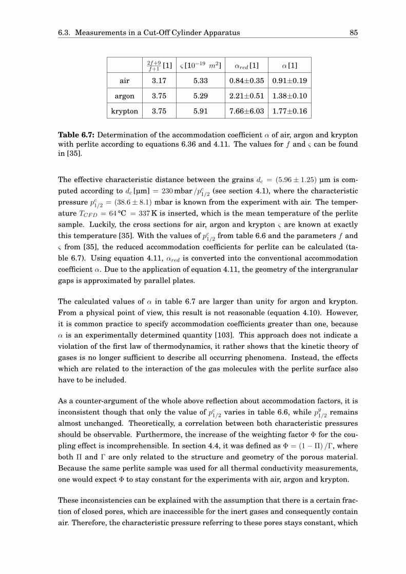
6.3. Measurements in a Cut-Off Cylinder Apparatus 85
2f+9f+1 [1] ς [10−19
m2] αred [1] α [1]
air 3.17 5.33 0.84±0.35 0.91±0.19
argon 3.75 5.29 2.21±0.51 1.38±0.10
krypton 3.75 5.91 7.66±6.03 1.77±0.16
Table 6.7: Determination of the accommodation coefficient α of air, argon and kryptonwith perlite according to equations 6.36 and 4.11. The values for f and ς can be foundin [35].
The effective characteristic distance between the grains dc = (5.96± 1.25) µm is com-puted according to dc [µm] = 230mbar /pc1/2 (see section 4.1), where the characteristicpressure p
c1/2 = (38.6± 8.1) mbar is known from the experiment with air. The temper-
ature TCFD = 64 °C = 337K is inserted, which is the mean temperature of the perlitesample. Luckily, the cross sections for air, argon and krypton ς are known at exactlythis temperature [35]. With the values of pc1/2 from table 6.6 and the parameters f andς from [35], the reduced accommodation coefficients for perlite can be calculated (ta-ble 6.7). Using equation 4.11, αred is converted into the conventional accommodationcoefficient α. Due to the application of equation 4.11, the geometry of the intergranulargaps is approximated by parallel plates.
The calculated values of α in table 6.7 are larger than unity for argon and krypton.From a physical point of view, this result is not reasonable (equation 4.10). However,it is common practice to specify accommodation coefficients greater than one, becauseα is an experimentally determined quantity [103]. This approach does not indicate aviolation of the first law of thermodynamics, it rather shows that the kinetic theory ofgases is no longer sufficient to describe all occurring phenomena. Instead, the effectswhich are related to the interaction of the gas molecules with the perlite surface alsohave to be included.
As a counter-argument of the whole above reflection about accommodation factors, it isinconsistent though that only the value of p
c1/2 varies in table 6.6, while p
g1/2 remains
almost unchanged. Theoretically, a correlation between both characteristic pressuresshould be observable. Furthermore, the increase of the weighting factor Φ for the cou-pling effect is incomprehensible. In section 4.4, it was defined as Φ = (1−Π) /Γ, whereboth Π and Γ are only related to the structure and geometry of the porous material.Because the same perlite sample was used for all thermal conductivity measurements,one would expect Φ to stay constant for the experiments with air, argon and krypton.
These inconsistencies can be explained with the assumption that there is a certain frac-tion of closed pores, which are inaccessible for the inert gases and consequently containair. Therefore, the characteristic pressure referring to these pores stays constant, which

86 Chapter 6. Laboratory Measurements
matches the observation for pg1/2. In addition, the overall thermal conductivity λg + λc
is increased due to the higher continuum thermal conductivity of air compared to argonand krypton. The only possibility of the fitting procedure to account for this increaseis to raise the weighting factor Φ. Thus, the observed effects would become reasonable.However, this assumption of closed pores containing air is not further justified. For clar-ification, microscopic examinations or similar investigations of the material structurewould be necessary.
Nevertheless, it has to be appreciated that the model for the pressure-dependent part ofthe effective thermal conductivity, which was used in this thesis, is able to represent themeasured values of both the parallel plate setup and the cut-off cylinder apparatus. Ithas to be kept in mind that other models, which are more sophisticated and precise froma theoretical point of view, could not achieve a complete agreement with experimentaldata [42]. Obviously, there is still a discrepancy between theory and experiments, espe-cially regarding the coupling effect in porous materials. Therefore, it is a great successto obtain an excellent agreement between the measurement values and the fitting modelwith only three parameters, although the physical interpretation of these parameters isnot fully reasonable.
6.4 Determination of the Moisture Content
As a last important experiment, the moisture content w of TECHNOPERL ® - C 1,5 wasmeasured, which is defined as:
w =mwater
msample(6.37)
For this purpose, the METTLER TOLEDO HR 83 halogen moisture analyzer was used,which is a special measuring instrument for the experimental determination of w. Itsmain component is a high precision balance, on which the sample is placed (figure 6.17).The investigated perlite sample had been exposed to the humidity of ambient air for aduration of several days. During the measurement in the moisture analyzer, the spec-imen is heated up by the radiation emitted from a halogen lamp. As a consequence,moisture which is contained in the material, evaporates and escapes. The temperatureof the baking-out process can be adjusted by varying the radiation intensity and wasset to T = 200 °C. The time evolution of the sample weight is recorded by the device(figure 6.18). According to the operation manual, it can be measured with an accuracyof ∆m = 1mg [104]. A total duration of t = 2h was chosen for the experiment.

6.4. Determination of the Moisture Content 87
The following results can be derived from the measurement:
• From the initial mass mi = 1 g and the final mass mf = 0.986 g, the moisturecontent can be calculated:
w =mwater
msample=
mi −mf
mi= (1.4± 0.2) % (6.38)
This result is in good agreement with w = 1.7%, which was obtained in section 6.2.At such low values of w, the only possible heat transfer mechanism connected tomoisture, which can have an effect in practice, is gaseous conduction due to watervapor. This impact is relatively harmless, because the thermal conductivities ofwater vapor and air are almost identical (λwv = 0.025 W/mK [34]). The two detri-mental effects of moisture were already excluded in section 4.6: Pore diffusion cannot happen as a consequence of the phase diagram of water, and flooding of poreswith liquid water requires the perlite insulation to be completely wet.
• According to figure 6.18, the sample is already completely dry after a durationof 20 minutes, because its weight is equal to the final value and does not changesignificantly anymore. This result is important for the thermal conductivity mea-surements in the parallel plate setup and in the cut-off cylinder apparatus, wherethe samples were baked out prior to the experiments. Although the ratio of samplesurface against volume was worse and the temperature was only T = 150 °C, thesamples can be assumed to be completely dry, because the baking-out process wasperformed in vacuum and the duration was several hours.
Figure 6.17: Measurement principle for the experimental determination of the mois-ture content.

88 Chapter 6. Laboratory Measurements
Figure 6.18: Weight of a perlite sample as a function of time for the determination ofthe moisture content.

89
Chapter 7
Heat Loss Measurements on aReal-Size Storage Prototype
In the framework of the research project at ZAE BAYERN about super-insulated long-term hot water storages, a real-size prototype tank was constructed by the project part-ner HUMMELSBERGER GMBH in Mühldorf in order to perform a variety of experimentsunder real conditions. During this thesis, heat loss measurements at the storage havebeen accomplished to determine the thermal conductivity of the vacuum super insula-tion in a real application.
7.1 Tank Layout and Measurement Setup
With respect to its schematic layout, the prototype is similar to the liquid gas storagetank described in section 5.2: The hot water is stored in the inner cylindrical container,which is fixed in the outer tank by a special suspension device (figure 5.2). Both contain-ers are made of steel. The annular gap is filled with perlite (TECHNOPERL ® - C 1,5)and evacuated. In addition, the prototype tank is also equipped with several high-gradesteel pipeline connections to load and discharge the water container. Furthermore, astratification device, which was mentioned in chapter 1, is installed. Figure 7.1 shows aphotograph and a sketch of the storage tank.
For the construction, large steel plates were bent to cylinders and subsequently cov-ered with torispherical heads on their top and bottom. The different components weremerged by welding. The heights of the tanks are Htot,in = 5.58m and Htot,out = 5.98m,and the respective diameters are Din = 2m and Dout = 2.4m. Thus, the annular gapbetween inner and outer container, which is equal to the insulation thickness, has aconstant value of dgap ≈ 0.2m, also in the region of the torispherical heads. In fact,dgap is slightly smaller, because the wall thickness of the containers has to be taken intoaccount. All relevant dimensions of the prototype including the lengths of the supplypipelines are listed in table 7.1.
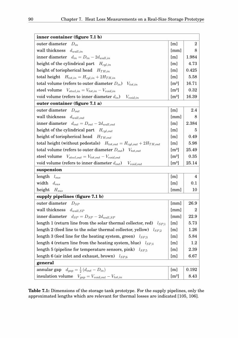
90 Chapter 7. Heat Loss Measurements on a Real-Size Storage Prototype
inner container (figure 7.1 b)outer diameter Din [m] 2wall thickness dwall,in [mm] 8inner diameter din = Din − 2dwall,in [m] 1.984height of the cylindrical part Hcyl,in [m] 4.73height of torispherical head HTH,in [m] 0.425total height Htot,in = Hcyl,in + 2HTH,in [m] 5.58total volume (refers to outer diameter Din) Vtot,in [m³] 16.71steel volume Vsteel,in = Vtot,in − Vvoid,in [m³] 0.32void volume (refers to inner diameter din) Vvoid,in [m³] 16.39outer container (figure 7.1 a)outer diameter Dout [m] 2.4wall thickness dwall,out [mm] 8inner diameter dout = Dout − 2dwall,out [m] 2.384height of the cylindrical part Hcyl,out [m] 5height of torispherical head HTH,out [m] 0.49total height (without pedestals) Htot,out = Hcyl,out + 2HTH,out [m] 5.98total volume (refers to outer diameter Dout) Vtot,out [m³] 25.49steel volume Vsteel,out = Vtot,out − Vvoid,out [m³] 0.35void volume (refers to inner diameter dout) Vvoid,out [m³] 25.14suspensionlength lsus [m] 4width dsus [m] 0.1height Hsus [mm] 10supply pipelines (figure 7.1 b)outer diameter DSP [mm] 26.9wall thickness dwall,SP [mm] 2inner diameter dSP = DSP − 2dwall,SP [mm] 22.9length 1 (return line from the solar thermal collector, red) lSP,1 [m] 5.73length 2 (feed line to the solar thermal collector, yellow) lSP,2 [m] 1.26length 3 (feed line for the heating system, green) lSP,3 [m] 5.84length 4 (return line from the heating system, blue) lSP,4 [m] 1.2length 5 (pipeline for temperature sensors, pink) lSP,5 [m] 2.39length 6 (air inlet and exhaust, brown) lSP,6 [m] 6.67generalannular gap dgap =
12 (dout −Din) [m] 0.192
insulation volume Vgap = Vvoid,out − Vtot,in [m³] 8.43
Table 7.1: Dimensions of the storage tank prototype. For the supply pipelines, only theapproximated lengths which are relevant for thermal losses are indicated [105, 106].

7.1. Tank Layout and Measurement Setup 91
Figure 7.1: Layout of the real-size storage tank prototype: Photograph of the tank (a),sketch of the inner container with supply pipelines and stratification device (b).
Temperature Measurement
14 Pt-1000 sensors are installed at different positions in the inner and outer container.6 sensors for measuring the water temperature (T1 to T6) are attached to the innersurface of a special supply pipeline, which is depicted pink in figure 7.1 b. The sensorsare positioned equally-spaced over the whole height of the prototype (table 7.2). Another6 sensors (T9 to T14) are located at the exterior surface of the outer container at the sameheights, so that each of the inner sensors has its respective counterpart. Further sensorsare mounted in the supply pipeline at a position near the bottom of the inner containerwithin the perlite insulation (T7) and on top of the outer container (T8). However, thesetemperatures are not relevant for the determination of the thermal conductivity fromthe heat loss measurement.
sensors T1 and T9 T2 and T10 T3 and T11 T4 and T12 T5 and T13 T6 and T14
height [m] 0.815 1.685 2.555 3.425 4.295 5.165
Table 7.2: positions of Pt-1000 temperature sensors, measured from the bottom of theouter container.

92 Chapter 7. Heat Loss Measurements on a Real-Size Storage Prototype
Because the electrical resistance of the Pt-1000 sensors is much larger than the re-sistance of the cables, temperatures are measured using the two-wire technique. Theassociated error is around ∆T = 1K. However, this error can be neglected for the de-termination of the thermal conductivity of the vacuum super insulation, because it isidentical for all sensors (the lengths of the electrical supply cables are virtually equal)and only temperature differences are needed for the calculation (see section 7.2). An ad-ditional error for the temperature measurement arises from the fact that the pipeline, inwhich the sensors T1 to T7 are attached, is filled with air. As a consequence of convectioninside the pipe, the temperature of the sensors T1 to T6 may differ from the real wa-ter temperature at the respective height. This error is also irrelevant though, becausethe water inside the tank was heated up to a homogeneous temperature of T = 90 °Cfor the heat loss measurement. Convection inside the pipe can only occur if there is asufficiently pronounced temperature difference along its height.
Pressure Measurement
Two vacuum flange connections are available, one at the bottom and one at the toptorispherical head of the outer container. Initially, four pressure sensors were connected,both a capacitive sensor and a Pirani gauge [96] at both the upper and the lower position.From comparing the two capacitive sensors at a vacuum pressure of p ≈ 0.01mbar, itshowed that there were no pressure differences between the top and the bottom regionof the insulation. Therefore, the lower capacitive sensor was dismounted again. BecausePirani gauges are much less accurate, the capacitive sensor at the top of the prototypetank is used for the pressure measurement. As indicated in section 6.3, this type ofsensor has a typical error of around 1 %.
Perlite Filling
During the process of filling the annular gap of the storage prototype with perlite, thecompressibility of the material, which was already mentioned in the sections 4.3 and 5.5,became notable to a great extent: In total, 779kg of TECHNOPERL ® - C 1,5 were filledinto the annular gap with a total void volume of Vgap = 8.43m³ (table 7.1). The resultingbulk density is:
ρ =m
Vgap= 92.4
kgm³
(7.1)
7.2 Presentation and Evaluation of Measurement Results
Heat Loss Measurement with Air at p = 0.08 mbar
The first important experiment, which was performed at the storage tank prototype, wasthe determination of the thermal conductivity λeff of the vacuum super insulation. Theconcept of the experiment was to measure the rate of temperature decrease dTwater/dt ofthe stored water and the ambient temperature Ta. If the total integral heat capacity Ctot

7.2. Presentation and Evaluation of Measurement Results 93
of the inner container and the shape factor Stot of the overall tank geometry are known,λeff can be calculated according to:
CtotdTwater
dt= Q = λeffStot (Twater − Ta) (7.2)
Theoretically, this method is only correct if Twater and dTwater/dt are determined at asingle point in time, because Twater decreases exponentially (equation 1.1). In practicehowever, the derivative can be replaced by ∆Twater/∆t, where ∆t is an extended timeinterval with a constant temperature decrease (linear approximation). The calculationprocedure is described in detail below, because equation 7.2 includes some simplifica-tions and is only suitable to illustrate the measurement principle.
The temperature decrease was measured over a period of 240 hours starting on Decem-ber 10, 2010 at 12:00 a.m. (midnight). A few days prior to the measurement, the waterinside the storage tank was heated up to T = 90 °C using a specially designed heatingstation, which was connected to the supply pipelines for the solar collector. At the end ofthis process, a homogeneous temperature of T1 = T2 = ... = T6 = 90 °C was reached. Forthe evaluation of the heat loss measurement, the average temperature of the sensors T1
to T6 was calculated and is shown in figure 7.2 as a function of time. During the mea-surement interval, the mean vacuum pressure in the insulation was p = 0.0833mbar.The rate of temperature decrease is obtained from the linear fit (red line):
∆Twater
∆t= 2.69 · 10−6 K
s(7.3)
The statistical error of the fit is more than three orders of magnitude smaller and there-fore neglected.
Figure 7.2: Decrease of the average water temperature for the heat loss measurement.

94 Chapter 7. Heat Loss Measurements on a Real-Size Storage Prototype
In the next step, the total integral heat capacity Ctot is determined. For its calculation,three contributions have to be taken into account:
• The largest fraction of Ctot is the heat capacity Cwater = cwatermwater of the storedwater. During the filling process of the inner container, a water mass of mwater =
15, 537kg was measured. With the specific heat capacity cwater = 4, 187J/kgK [72],one arrives at Cwater = 65.05 · 106 J/K. However, this quantity contains an error: AtT = 90 °C, the density of water is given by ρwater = 965.3kg/m³ [107]. Therefore,the measured value for mwater corresponds to a volume of Vwater = 16.1m³, whichis less than the void volume of the inner tank Vvoid,in = 16.4m³ (table 7.1). Thismeans, that either the container has not been completely filled with water, or themeasurement of the water mass has been inaccurate. The systematic error is as-sumed to be equal to the difference of Vvoid,in−Vwater = 0.3m³. Converted into heatcapacity, one arrives at ∆Cwater = 1.21 · 106 J/K.
• The temperature of the steel container is practically identical to the water tem-perature, which causes another considerable contribution of Ctot. From Csteel =
csteelρsteelVsteel,in and the values csteel = 477J/kgK [108], ρsteel = 8, 000kg/m³ [108]and Vsteel,in = 0.32m³ (table 7.1), one obtains Csteel = 1.22 · 106 J/K.
• Finally, also the heat capacity of the perlite inside the annular gap has to be con-sidered. However, this contribution has to be weighted by a factor of 1/2, be-cause the average temperature Tperlite = (Twater + Ta) /2 only decreases by 0.5Kif the water temperature Twater drops by 1K and the ambient temperature Ta
stays constant. With cperlite = 900J/kgK [109], ρperlite = 92.4kg/m³ (equation 7.1)and Vgap = 8.43m³ (table 7.1), the contribution of perlite is equal to Cperlite =
cperliteρperliteVgap/2 = 0.35 · 106 J/K. On a sidenote, the linear approximation Tperlite =
(Twater + Ta) /2 is valid, because the gap size dgap (table 7.1) is much smaller thanthe diameter Din of the inner tank and therefore the geometry can be approxi-mated by parallel plates (see section 2.1).
Summing up the three fractions, one arrives at:
Ctot = Cwater + Csteel + Cperlite = (66.6± 1.2) · 106JK
(7.4)
With this result, the heat loss of the stored water can be calculated according to:
Qtot = Ctot∆Twater
∆t= (179.1± 3.2) W (7.5)
For the further evaluation, it has to be taken into account that the total rate of heatloss Qtot is not equal to the heat flux Qperlite through the evacuated perlite insulation,because it also includes thermal losses Qloss via the supply pipelines and the suspensiondevice. In a separate investigation [105], the thermal losses were calculated from the

7.2. Presentation and Evaluation of Measurement Results 95
relevant dimensions (table 7.1) using numerical methods. The result of this examinationis Qloss = 2.4W. It is in good agreement with the following approximation:
Qloss,approx = Qsuspension + Qpipelines
= 2λsteeldsusHsus
lsus∆T +
6
i=1
λHGS
D
2SP − d
2SP
π
4lSP,i∆T
= 2.3W + 0.5W = 2.8W (7.6)
For this calculation, the values λsteel = 50W/mK [110], λHGS = 15W/mK [102] and∆T = 90K were used.
As a consequence of the determination of Qloss, the heat flux through the insulation isgiven by:
Qperlite = Qtot − Qloss = (176.7± 3.2) W (7.7)
Now, equation 7.2 suggests to determine the total shape factor of the storage prototypeand to calculate λeff from the measured temperature difference ∆T = Twater −Ta. How-ever, ∆T is not constant everywhere. During the heat loss measurement, the water inthe top region of the inner container was around 3K hotter than the water at the bottom.Therefore, the heat flux Qperlite is divided into three parts, which is more precise:
Qperlite = Qtop + Qcyl + Qbottom
= λeff
STH∆Ttop +
2πHcyl,in
ln (dout/Din)∆Tcyl + STH∆Tbottom
(7.8)
The major fraction of Qperlite flows through the cylindrical part of the storage tank.It is denoted with Qcyl and can be calculated according to equation 2.4. The relevantdimensions Hcyl,in, dout and Din can be read off from table 7.1. At the top and bottomboundaries, the heat transfer rates Qtop and Qbottom through the arrangement of thetorispherical heads have to be calculated. For an exact evaluation, equation 2.6 hasto be used, which requires the determination of the shape factor STH . Thus, the fourparameters ∆Ttop, ∆Tcyl, ∆Tbottom and STH still have to be quantified in order to obtainthe effective thermal conductivity of the insulation.
The temperature differences can be determined relatively easy from the measured tem-peratures T1 to T6 and T9 to T14. First, the values are averaged over the total measure-ment interval of 10 days to obtain the mean temperatures T1 to T6 and T9 to T14. Thequantity ∆Ttop is then calculated from T1 and T9, which are the relevant temperaturesat the top region of the storage prototype:
∆Ttop = T1 − T9 = 89.7K (7.9)

96 Chapter 7. Heat Loss Measurements on a Real-Size Storage Prototype
In analogy, T6 and T14 are used for the bottom region:
∆Tbottom = T6 − T14 = 86.2K (7.10)
For the cylindrical part, the values from the remaining sensors are averaged:
∆Tcyl =1
4
T2 + T3 + T4 + T5 − T10 − T11 − T12 − T13
= 89.2K (7.11)
The calculation of the shape factor STH is more difficult. Initially, the geometry of thetorispherical heads, which consists of several radii and heights (figure 7.3) is approxi-mated by spherical caps with a single radius. The arrangement of the two torisphericalheads from the inner and the outer container according to the approximation is shownin figure 7.4. The dimensions r1, r2, d and h from figure 7.4 are defined according to thegeometry of the storage prototype (table 7.1):
r1 = 1m r2 = 1.2m d = 0.2m h = 0.4m (7.12)
Figure 7.3: Dimensioning of torispherical heads according to DIN 28011 [111, 112].
Figure 7.4: Approximation of the shape factor STH .

7.2. Presentation and Evaluation of Measurement Results 97
Subsequently, the missing geometrical quantities are calculated:
R21 = l
2 + r21 = (R1 − h)2 + r
21 ⇒ R1 =
h2 + r
21
2h= 1.45m
R2 = R1 + d = 1.65m
l = R1 − h = 1.05m
sinϕ =r1
R1⇒ ϕ = 43.6° (7.13)
Now, there are three possibilities to calculate S from the approximated geometry:
• The area A of a spherical cap is given by [113]:
A = 2πR2 (1− cosϕ) (7.14)
Therefore, the approximation for parallel plates (equation 2.3) can be applied, us-ing the area A1 of the inner spherical cap as reference area:
Sapprox,1 =A1
d=
2πR21 (1− cosϕ)
d= 18.2m (7.15)
• In analogy, it is also possible to refer to the area A2 of the outer spherical cap:
Sapprox,2 =A2
d=
2πR22 (1− cosϕ)
d= 23.6m (7.16)
• Eventually, one can also use equation 2.5, which is valid for spherical geometries.Applying this method, the factor (1− cosϕ) /2 has to be included, because the ap-proximated shape factor Sapprox,3 must not refer to the whole surface of the sphere,but only to the fraction of the spherical cap:
Sapprox,3 =4π (1− cosϕ)
2
1R1
− 1R2
= 20.7m (7.17)
Because the deviations between the three different approximated shape factors are inthe range of up to 30 %, a numerical simulation has been done in order to obtain areliable result for STH . For this purpose, the exact geometry of the storage prototypeincluding the dimensioning of the torispherical heads (figure 7.3) has been modelledin SOLIDWORKS 2008, and the add-on COSMOSFLOWORKS 2008 has been used tocalculate the heat flux through the arrangement of the inner and outer torisphericalhead at a given thermal conductivity of the insulation and temperature difference [105].The numerical investigation yields:
STH,CFD = 23.6m (7.18)
It is a remarkable coincidence, that this result is identical to Sapprox,2, which has beencalculated from an approximation by parallel plates.
98 Chapter 7. Heat Loss Measurements on a Real-Size Storage Prototype
Finally, all relevant parameters are known, and the effective thermal conductivity of theevacuated perlite insulation (p = 0.08mbar) can be calculated by inserting the resultsfrom equations 7.7, 7.9 to 7.11 and 7.18 into equation 7.8:
λeff =Qperlite
STH∆Ttop +2πHcyl,in
ln(dout/Din)∆Tcyl + STH∆Tbottom
= (9.18± 0.17) · 10−3 WmK
(7.19)
This value is surprisingly low, because one would expect a solid thermal conductivityof λs = (14.7± 1.6) W/mK from the measurements in the parallel plate setup (equa-tion 6.15), which is already significantly higher than the total effective thermal conduc-tivity of the perlite insulation in the storage prototype. This result is interpreted asanother argument confirming the assumption on page 67, which states that the ther-mal resistances due to the solid structure were shorted by the high external pressureduring the experiments in the parallel plate apparatus. This supposition was alreadysupported by the estimation of the solid thermal conductivity from the measurements inthe cut-off cylinder device (section 6.3.2). Obviously, there are two different possibilitiesto create high bulk densities for perlite:
The material can be compressed by applying external pressure. As mentioned above,the solid structure is damaged in this case, which leads to the shorting of thermal resis-tances. Under these conditions, equation 6.15 can be used to calculate the solid thermalconductivity.
Another possibility is to compress the material by pouring and vibrations, which causesthe single perlite grains to arrange in a space-saving way (close-packing of spheres).Because the solid structure stays intact, the value of λs must be lower in this case. Thedensity dependency of the solid thermal conductivity is still assumed to be linear for thissituation. In order to determine λs (ρ), at least three data points are necessary. Fortu-nately, one experimental value is available from each of the measurements in Würzburg,Garching and Mühldorf:
• In the parallel plate device, the material was still uncompressed during the mea-surement at the lowest density (ρ = 55.2kg/m3). The corresponding solid ther-mal conductivity was λs = (2.46± 1.23) · 10−3 W/mK at the mean temperatureT = 361K (average values of all four measurements in figure 6.6).
• From the measurements in the cut-off cylinder apparatus at ρ = 68.2kg/m3 andT = 337K, a solid thermal conductivity of λs = (3.39± 1.27) · 10−3 W/mK was esti-mated (section 6.2.2).
• Finally, the value of λs at ρ = 92.4kg/m3 can be calculated from the heat lossmeasurement on the storage prototype. As derived above, the effective thermalconductivity of the insulation is λeff = (9.18± 0.17) · 10−3 W/mK (equation 7.19)at a pressure of p = 0.08mbar. As a first step, the radiative thermal conductivity

7.2. Presentation and Evaluation of Measurement Results 99
λr = (2.55± 0.25) · 10−3 W/mK is computed according to equation 6.10, where theradiation temperature Tr is calculated from the average values of the temperaturesT1 to T6 and T9 to T14. Subsequently, the contribution of gaseous conduction andcoupling is determined from equation 6.14. For the parameters p
g1/2, p
c1/2 and Φ,
the values from table 6.4 are inserted, because the measurement in the cut-offcylinder apparatus better represents the unmodified material with the originalpore size. The result is λg + λc = (1.53± 0.08) · 10−3 W/mK. For this calculation,the continuum thermal conductivity λ0 = 27.3 · 10−3 W/mK is used [34]. This is thecorrect value at the average temperature of the perlite insulation T = 315K, whichis the arithmetic mean of the temperatures T1 to T6 and T9 to T14. Subtractingλr and λg + λc from λeff , one arrives at λs = (5.1± 0.5) · 10−3 W/mK. This valuereally represents the solid thermal conductivity of TECHNOPERL ® - C 1,5 withoutexternal pressure, because the pressure acting on the perlite layer at the bottomof the tank due to the weight of the higher layers is only pext = ρperlit Vgap g/Aring =
58mbar, which is much less than the pressure load of pext = 1.05bar during themeasurement in the parallel plate apparatus. For this calculation, the area Aring =d2out −D
2in
π/4 has been used.
In figure 7.5, these values of λs without external pressure are shown as a function ofdensity. Although the errors are relatively large, the linear correlation is clearly visible.The temperature dependency of λs is neglected, because it showed during the measure-ments in the parallel plate apparatus, that this effect is relatively small. Furthermore,the individual data points in figure 7.5 were measured at similar temperatures.
Figure 7.5: Solid heat conductivity as a function of density without external pressure.

100 Chapter 7. Heat Loss Measurements on a Real-Size Storage Prototype
From the linear fit in figure 7.5, one obtains:
λs =
(0.0709± 0.0002) · ρ
kg
m³
− (1.4499± 0.0135)
· 10−3 W
mK(7.20)
Since equation 7.20 represents an intact solid structure, it is much more suitable thanequation 6.15 for the calculation of λs under practical conditions.
Heat Loss Measurement with Krypton at p = 7.6 mbar
In a further experiment, the annular gap between both containers was completely evacu-ated and subsequently filled with krypton. Just like before, the water inside the storagewas heated up to a homogeneous temperature (T = 95 °C), and the heat loss ∆Twater/∆t
was measured for a total duration of 7 days, starting on May 24, 2010 at 12:00 a.m.(midnight). During this period, the average pressure within the perlite insulation wasp = 7.598mbar. The other measured quantities, which are relevant for the determina-tion of the effective thermal conductivity, are:
∆Twater/∆t = 5.48 · 10−6 Ks
∆Ttop = 73.5K ∆Tbottom = 69.0K ∆Tcyl = 72.8K (7.21)
According to equation 7.5, this corresponds to a total heat loss of Qtot = (365.3± 6.6) W.The thermal losses Qloss = 1.9W due to the supply pipelines and the suspension deviceare smaller, because the temperature differences were lower compared to the measure-ment with air as a consequence of the higher ambient temperature in May. Therefore,the rate of heat transfer through the perlite insulation is given by Qperlite = (363.4± 6.6) W(equation 7.7). By inserting this result into equation 7.19, the effective thermal con-ductivity of the perlite insulation under the effect of krypton at p = 7.6mbar can becalculated:
λeff = (23.1± 0.4) · 10−3 WmK
(7.22)
With λr = (3.0± 0.3) · 10−3 W/mK, which has been computed according to equation 6.10with the measured temperatures T1 to T6 and T9 to T14, and λs = (5.1± 0.5) · 10−3 W/mK(see figure 7.5), this value is equivalent to:
λg + λc = (15.0± 1.2) · 10−3 WmK
(7.23)
This result is in perfect agreement with the krypton measurements in the cut-off cylin-der apparatus: With the mean perlite temperature T = 55.5 °C during the heat lossmeasurement in the storage prototype, the continuum thermal conductivity of kryptonis given by λ0 = 10.3 · 10−3 W/mK [34]. From a calculation of λg + λc according to equa-tion 6.30 with this value for λ0 and the parameters p
g1/2, p
c1/2 and Φ from table 6.6, one
obtains λg + λc = (14.9± 2.3) · 10−3 W/mK.

7.2. Presentation and Evaluation of Measurement Results 101
Measurement of the Leakage Rate
Another important experiment for the practical application of vacuum super insulationis the determination of the leakage rate χ of the storage prototype. If the vacuum pres-sure increases over time, the insulation deteriorates due to an increment of λg and λc.For the measurement of χ, the pressure inside the annular gap was recorded over a totalduration of 83 days, from December 15, 2010 to March 8, 2011. The experimental datais shown in figure 7.6. Because pressure is correlated to temperature according to theideal gas law (pV/T = NkB), the values have been normalized:
p (t) =T
T (t)p (t) (7.24)
The mean temperature T has been determined from averaging over the whole measure-ment interval and over all temperatures T1 to T6 and T9 to T14. From the linear fit (redline in figure 7.6), one obtains the pressure increase p:
p = 2.70 · 10−9 mbars
= 2.33 · 10−4 mbard
= 0.085mbar
a(7.25)
With the insulation volume Vgap = 8.43m³, the leakage rate can be calculated:
χ = pVgap = 2.28 · 10−5 mbar ls
(7.26)
Figure 7.6: Determination of the leakage rate of the storage prototype.

.

103
Chapter 8
Summary of the ExperimentalResults and Conclusions
As a result of the experiments which were described in the two previous chapters, theeffective thermal conductivity λeff of TECHNOPERL ® - C 1,5 can be calculated at agiven pressure, temperature and density. This knowledge is important for the practicalapplication of vacuum super insulation in hot water storages. Furthermore, approachesto minimize λeff can be formulated.
8.1 Calculation of the Effective Thermal Conductivity forPractical Purposes
According to section 4.5, there are four mechanisms that contribute to the effective ther-mal conductivity: radiative heat transport, solid conduction, gas conduction and thecoupling effect:
λeff = λr + λs + λg + λc (8.1)
For the radiative thermal conductivity λr (T, ρ) as a function of temperature and density,the following relation can be used (sections 4.3 and 6.1):
λr (T, ρ) =16σT 3
r
3ρe∗(Tr)(8.2)
In equation 8.2, σ = 5.6704 · 10−8 W/m2K4 is the Stefan-Boltzmann constant. Further-more, the radiation temperature Tr occurs (see section 4.3), which is defined as:
Tr =3
1
4
T21 + T
22
(T1 + T2) (8.3)
T1 and T2 are the temperatures of the insulation boundaries. In the case of a cylin-drical storage tank, T1 can by approximated by the water temperature in the inner

104 Chapter 8. Summary of the Experimental Results and Conclusions
container, and T2 is practically identical with the ambient temperature. The extinctione∗(Tr) has been determined experimentally (section 6.1). In the temperature interval
between 300K ≤ Tr ≤ 450K, it can be calculated from a quadratic approximation ac-cording to:
e∗(Tr) =
5.32 · 10−4 ·Tr[K]2 − 0.4503 ·Tr[K] + 130.31
m²kg
± 4m²kg
(8.4)
For the solid thermal conductivity λs (T, ρ), a linear dependency on density has beenobserved:
λs (ρ) =
(0.0709± 0.0002) · ρ
kg
m³
− (1.4499± 0.0135)
· 10−3 W
mK(8.5)
Equation 8.5 is only valid if the material is compressed by its own weight or by vibra-tions, which cause the single perlite grains to arrange in a close packing of spheres(see section 7.2). If the compression is achieved by external pressure, the solid struc-ture is damaged and thermal resistances are shorted. In this case, equation 6.15 hasto be used. The temperature dependency of λs, which has been expected according tosection 4.2, has not been observed in the experiments. It is assumed that this effect isnegligibly small.
The gaseous thermal conductivity λg (T, p) at a given vacuum pressure and temperaturecan be calculated using the Sherman interpolation (section 4.1):
λg (T, p) =λ0 (T )
1 +pg1/2p
(8.6)
The characteristic half-value pressure pg1/2 has been determined experimentally for air,
argon and krypton and is shown in table 8.1. In addition, the temperature-dependentcontinuum thermal conductivity λ0 (T ) appears in equation 8.6. λ0 (T ) is depicted infigure 8.1 for a selection of gases and can be approximated using a second-order polyno-mial:
λ0 =A+B T [°C] + C T [°C]2
· 10−3 W
mK(8.7)
The constants A, B and C are listed in table 8.2.
Regarding the coupling thermal conductivity λc (T, p), the experiments in chapter 6 haveshown that the measured data can successfully be represented by the simplified cou-pling model, which was developed in section 4.4:
λc (T, p) = Φλ0 (T )
1 +pc1/2p
(8.8)
Again, the continuum thermal conductivity can be computed according to equation 8.7.The parameters Φ and p
c1/2 are included in table 8.1 for air, argon and krypton.

8.1. Calculation of the Effective Thermal Conductivity for Practical Purposes 105
gas pg1/2 [mbar] Φ [1] p
c1/2 [mbar]
air 1.38±0.07 0.54±0.03 38.6±8.1
argon 1.46±0.01 0.73±0.01 17.4±0.4
krypton 1.24±0.47 0.93±0.06 4.5±2.6
Table 8.1: Parameters for the calculation of λg and λc according to equations 8.6 and 8.8.
gas A [1] B [1] C [1]
air 24.17±0.02 0.075±0.001 (-2.88±0.14) · 10−5
argon 16.39±0.10 0.049±0.001 (-2.72±0.56) · 10−5
krypton 8.76±0.02 0.029±0.001 (-1.30±0.10) · 10−5
Table 8.2: Parameters for the calculation of λ0 according to equation 8.7.
Figure 8.1: Continuum thermal conductivity λ0 of selected gases as a function of tem-perature [34].

106 Chapter 8. Summary of the Experimental Results and Conclusions
8.2 Suggestion of Optimization Approaches
In the experimental part of this thesis (chapters 6 and 7), the dependencies of the ef-fective thermal conductivity on pressure, density, temperature and the type of fillinggas have been measured. As a consequence, different optimization approaches can besuggested with the aim to minimize λeff under practical conditions.
Minimization of λs and λr
Both the solid and the radiative thermal conductivity of TECHNOPERL ® - C 1,5 dependon density. λs increases linearly with ρ (equation 8.5), whereas λr decreases accordingto λr ∼ ρ
−1 (equation 8.2). Therefore, an optimum density ρopt exists, at which the sumλr+λs attains a minimum value. Because λr also depends on the radiation temperature,ρopt is a function of Tr, which is usually predetermined by the application. The temper-ature dependency of λs is neglected (see section 6.2.2). In figure 8.2, the sum of λr + λs
is plotted against ρ at different radiation temperatures. The blue curve with Tr = 325Krefers to the storage of hot water for solar thermal applications (T1 = 100 °C, T2 = 0 °C).
The optimum density can be calculated using the conventional method for the determi-nation of extremal values:
d (λr + λs)
dρ= − 16σT 3
r
3ρ2e∗ (Tr)+As
!= 0
⇒ ρopt =
16σT 3
r
3Ase∗ (Tr)
(8.9)
In equation 8.9, As = 0.0709 · 10−3 W m2/K kg is the first coefficient for the linear density
dependency of λs (see equation 8.5). The optimum density as a function of the radiationtemperature Tr is depicted in figure 8.3.
With respect to the solar thermal application (Tr = 325K), it shows that the optimumdensity is at ρopt = 60.4kg/m³. It is questionable whether this value can be reached inpractice, because the self-adapted bulk density in the storage prototype is considerablyhigher (ρ = 92.4kg/m3). However, it has to be said that the influence of ρ is not verypronounced at Tr = 325K, which can be demonstrated by figure 8.2 (blue curve): In thewhole interval from 50kg/m³ ≤ ρ ≤ 95kg/m³, the sum of radiative and solid thermal con-ductivity only changes by 1 · 10−3 W/mK. For the application of vacuum super insulationin this temperature range, the bulk density of ρ = 92.4kg/m3 is still acceptable, becauseλr + λs is only slightly above the minimum value.

8.2. Suggestion of Optimization Approaches 107
Figure 8.2: Sum of radiative and solid thermal conductivity as a function of densityaccording to equations 8.2 and 8.5.
Figure 8.3: Optimum density ρopt as a function of radiation temperature according toequation 8.9.

108 Chapter 8. Summary of the Experimental Results and Conclusions
Minimization of λg and λc
Both gas conduction and the coupling effect depend on temperature and pressure (seeequations 8.6 and 8.8). Like before, the temperature, which determines the continuumthermal conductivity λ0, is given by the application. It is obvious that an increase ofvacuum pressure, caused by the leakage rate χ, leads to an enhancement of λg + λc. Inpractice, it is therefore necessary to keep the vacuum pressure as low as possible duringthe lifetime of a hot water storage tank, which is around 20 years.
For the conventional application with air as filling gas, this effect is illustrated in fig-ure 8.4, where the time development of λg + λc is depicted using the leakage rate χ asa parameter. The values for λg + λc have been calculated from equations 8.6 and 8.8with the parameters p
g1/2, Φ and p
c1/2 from table 8.1. For normalization, λg + λc has been
divided by λ0:λg + λc
λ0=
1
1 +pg1/2p(t)
+Φ
1 +pc1/2p(t)
(8.10)
The pressure p (t) is calculated according to:
p (t) = p0 +χt
Vgap(8.11)
In this equation, Vgap = 8.43m³ is the insulation volume of the prototype and p0 is theinitial pressure, which is set to p0 = 0.01mbar. This value is a suitable compromise forpractical applications, because it can be achieved with a moderate technical effort, butgas conduction and coupling is already sufficiently suppressed (λg+λc = 2 · 10−4 W/mK).
The red curve in figure 8.4 with χ = 2.3 · 10−5 mbar l/s refers to the storage prototype,which is most likely the worst case regarding the leakage rate. It is assumed that χ
can be reduced by a factor of 5 for commercially available storages, because these tanksdo not have to be equipped with measurement instrumentation (pressure sensors) andthe number of vacuum connections can be decreased. However, for χ = 5 · 10−6 mbar l/s(green curve), the value of λg + λc is still relatively high after 20 years. With T = 50 °Cand λ0 = 27.9 · 10−3 W/mK [34], one obtains λg + λc = 6 · 10−3 W/mK. A further reductionof the leakage rate (blue and purple curve) is desirable.
Lowering the initial pressure (for example to p0 = 0.001mbar) is not very effective forthe long-time consideration of λg + λc. If χ = 2.3 · 10−5 mbar l/s, the pressure reachesp = 0.01mbar after only 40 days. Even at the lowest indicated leakage rate of χ =
10−6 mbar l/s, the pressure rises to p = 0.01mbar after three years.
If the leakage rate cannot be reduced to a sufficiently low value, another option to main-tain low thermal conductivities would be to re-evacuate the perlite insulation in regularintervals of several years.

8.2. Suggestion of Optimization Approaches 109
Figure 8.4: Development of λg + λc over the typical lifetime of a hot water storage tankat different leakage rates χ according to equation 8.10.
Utilization of Inert Gases
A further theoretical possibility to maintain low effective thermal conductivities duringthe lifetime of the storages in spite of leakages is the utilization of krypton, which ischaracterized by its low heat conductivity both in the continuum and in the regime offree molecular flow (see section 4.1). The application of argon is not suggestive, becausethe thermal conductivity of the perlite insulation under the effect of argon is too closeto the value of air (see figure 6.16). It is now examined, whether the usage of kryptonis a reasonable option in practice. Therefore, a relation for the pressure dependency ofthe total thermal conductivity of a gas mixture is necessary. Initially, only gas conduc-tion in the pores is considered, and the coupling effect will be treated by analogy later.From equation 4.13, a relation for the total continuum thermal conductivity λ
tot0 of a gas
mixture is known, which is now applied to the mixture of air and krypton:
λtot0 =
pairλair0 + pkrλ
kr0
pair + pkr(8.12)
In this equation, pair and pkr are the partial pressures of air and krypton, and λair0 and
λkr0 are the continuum thermal conductivities. As demonstrated by figure 4.3, λ
tot0 is
always larger than λkr0 and smaller than λ
air0 . In the regime of free molecular flow, this
can no longer be valid. Because collisions between the gas molecules can be neglected

110 Chapter 8. Summary of the Experimental Results and Conclusions
and the particles move freely between the boundary walls, the two components of thegas mixture represent a parallel connection of thermal resistances (equation 4.30). Ac-cordingly, the individual thermal conductivities have to add up:
λtotFM = λ
airFM + λ
krFM =
pairλair0
pg,air1/2
+pkrλ
kr0
pg,kr1/2
(8.13)
The relation λairFM = pairλ
air0 /p
g,air1/2 and the analog expression for krypton is obtained
from the low-pressure limit of the Sherman interpolation (equation 4.4). With p → 0
and consequently1 + p
g,air1/2 /pair
→ p
g,air1/2 /pair, one arrives at the above term.
Now, the quantity λtotIGP , which is the interpolation to general pressures (index IGP) of
the total thermal conductivity of a gas mixture, is calculated according to:
1
λtotIGP
=1
λtot0
+1
λtotFM
(8.14)
This approach corresponds to the Sherman interpolation for a pure, single-componentgas [35]. After inserting equations 8.12 and 8.13 and solving for λ
totIGP , one arrives at:
λtotIGP
λair0
=
pair + pkr
λkr0
λair0
pairp
g,kr1/2 + pkrp
g,air1/2
λkr0
λair0
(pair + pkr)pairp
g,kr1/2 + pkrp
g,air1/2
λkr0
λair0
+ p
g,air1/2 p
g,kr1/2
pair + pkr
λkr0
λair0
(8.15)
Again, the values are normalized by λair0 . This is possible, because the ratio λ
kr0 /λ
air0
only varies between 0.364 at T = 0 °C and 0.370 at T = 300 °C (compare figure 8.1).Therefore, λkr
0 /λair0 = 0.367 is set as a constant, which is exact for temperatures around
T = 125 °C and a very good approximation with a deviation of maximally 1 % for lowerand higher temperatures. The reason for this procedure is, that the calculated valuesfrom equation 8.15 are directly comparable to the curves in figure 8.4.
So far, only gas conduction in the pores has been considered. However, an analog expres-sion can easily be derived for the coupling thermal conductivity λ
tot,cIGP of the gas mixture
by replacing the terms λ0 with Φλ0 and the characteristic pressures pg1/2 with p
c1/2:
λtot,cIGP
λair0
=
pairΦair + pkrΦkr
λkr0
λair0
pairp
c,kr1/2 Φair + pkrp
c,air1/2 Φkr
λkr0
λair0
(pair + pkr)pairp
c,kr1/2 Φair + pkrp
c,air1/2 Φkr
λkr0
λair0
+ pc,air1/2 pc,kr1/2
pairΦair + pkrΦkr
λkr0
λair0
(8.16)
Now, the sum of gas conduction and coupling λg + λc can be calculated by adding equa-tions 8.15 and 8.16. For the characteristic pressures p1/2 and the weighting factorsΦ, the values from table 8.1 are inserted. Because the time-development of the totalthermal conductivity at different leakage rates is to be considered, the previously usedrelation has to be inserted for the partial pressure of air:
pair = pair,0 +χt
Vgap(8.17)

8.2. Suggestion of Optimization Approaches 111
Just like before, the void volume of the insulation is given by Vgap = 8.43m³, and theinitial pressure is set to pair,0 = 0.01mbar. The partial pressure of krypton is assumedto be constant over the whole time interval and is initially set to pkr = 1mbar. Althoughthe partial pressure of krypton in the ambient air is lower, the escape of krypton throughthe leakages due to diffusion can be neglected for two reasons:
• The krypton fraction of the atmosphere is in the range of 1 ppm [68], which cor-responds to a partial pressure of almost zero. The difference of partial pressures,which is the driving force for the pressure equalization, is thus given by the par-tial pressure pkr = 1mbar inside the insulation of the storage tank. This value ismuch smaller than the difference in the partial pressures of air, which is practi-cally equal to ∆pair = 1000mbar.
• The outward diffusion of krypton is obstructed by the opposingly directed flow ofambient air into the evacuated insulation volume.
Consequently, all revelant quantities are known, and the time development of the sumof gas conduction in the pores and coupling can be computed for the gas mixture ofair and krypton. The result for pkr = 1mbar is shown in figure 8.5. Another plot forpkr = 0.1mbar is depicted in figure 8.6.
Figure 8.5: Development of λg + λc over the lifetime of a hot water storage tank witha mixture of air and krypton according to equations 8.15 and 8.16. Due to the leakagerate χ, the composition of the gas mixture changes. The krypton pressure is set topkr = 1mbar. For comparison, the curves without krypton from figure 8.4 are depicted,too (dotted lines).
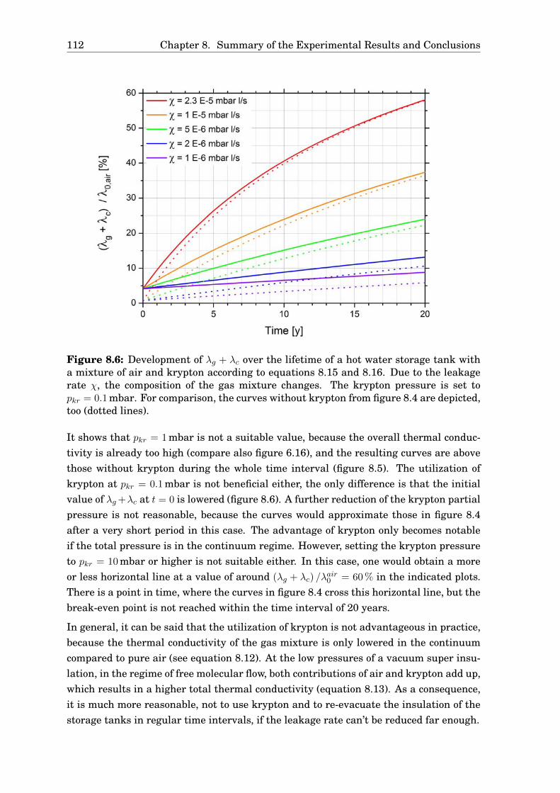
112 Chapter 8. Summary of the Experimental Results and Conclusions
Figure 8.6: Development of λg + λc over the lifetime of a hot water storage tank witha mixture of air and krypton according to equations 8.15 and 8.16. Due to the leakagerate χ, the composition of the gas mixture changes. The krypton pressure is set topkr = 0.1mbar. For comparison, the curves without krypton from figure 8.4 are depicted,too (dotted lines).
It shows that pkr = 1mbar is not a suitable value, because the overall thermal conduc-tivity is already too high (compare also figure 6.16), and the resulting curves are abovethose without krypton during the whole time interval (figure 8.5). The utilization ofkrypton at pkr = 0.1mbar is not beneficial either, the only difference is that the initialvalue of λg+λc at t = 0 is lowered (figure 8.6). A further reduction of the krypton partialpressure is not reasonable, because the curves would approximate those in figure 8.4after a very short period in this case. The advantage of krypton only becomes notableif the total pressure is in the continuum regime. However, setting the krypton pressureto pkr = 10mbar or higher is not suitable either. In this case, one would obtain a moreor less horizontal line at a value of around (λg + λc) /λair
0 = 60% in the indicated plots.There is a point in time, where the curves in figure 8.4 cross this horizontal line, but thebreak-even point is not reached within the time interval of 20 years.
In general, it can be said that the utilization of krypton is not advantageous in practice,because the thermal conductivity of the gas mixture is only lowered in the continuumcompared to pure air (see equation 8.12). At the low pressures of a vacuum super insu-lation, in the regime of free molecular flow, both contributions of air and krypton add up,which results in a higher total thermal conductivity (equation 8.13). As a consequence,it is much more reasonable, not to use krypton and to re-evacuate the insulation of thestorage tanks in regular time intervals, if the leakage rate can’t be reduced far enough.

113
Chapter 9
Outlook
The experimental investigation of the heat transport in evacuated perlite showed, thatthe single heat transfer mechanisms and their dependencies on pressure, density andtemperature can be described using common models and approaches. Due to this quan-tification, the effective thermal conductivity of TECHNOPERL ® - C 1,5 can be calcu-lated for practical applications, and optimization approaches can be suggested. How-ever, there is still motivation for future research and optimization.
Regarding the experiments, a first approach would be the improvement of the cut-offcylinder device, with the aim to reduce the leakage rate and to obtain minimum pres-sures lower than p = 0.02mbar. As a consequence, it would be possible to further inves-tigate the temperature dependency of solid conduction, and to measure the pressure-dependent part λg + λc of the effective thermal conductivity below p = 1mbar. In addi-tion, the geometry and the positioning of the installed cables can be optimized in orderto facilitate the calibration. Furthermore, a comparison between a parallel plate setupand a cylindrical geometry could be worthwile. In the experimental part of this the-sis, it has been notable that both measurement setups have their distinct benefits anddisadvantages. The comparison, which could also include spherical geometries, can beinteresting and helpful for thermal conductivity measurements in general.
With respect to the experimental results, a main topic for further analysis is the cou-pling effect. Although it showed that the model for perlite, which was developed insection 4.4, can reproduce the experiments, its physical interpretation is not completelyclarified. The increase of the weighting factor Φ, which was observed for argon andkrypton, was explained by the accommodation coefficient. To validate this approach,further measurements and also theoretical considerations are a possible subject of ad-ditional research. In addition, a microscopic inspection or a similar examination of thematerial structure is desirable, in order to verify the effective pore diameters and theintergranular space dimensions, which were calculated from the experimentally deter-mined characteristic pressures p1/2. This study could also clarify the effect of externalmechanical pressure on the material structure and the correlated solid thermal conduc-tivity.

114 Chapter 9. Outlook
Ultimately, other porous materials in combination with different filling gases can beinvestigated. Apart from perlite, there are several similar materials, for example di-atomaceous earth, expanded clay or aerogels. In addition to air, argon and krypton,one can think of the remaining inert gases helium, neon and xenon. Especially thelatter may be particularly interesting for insulation purposes due to its low thermalconductivity (compare figure 8.1). From the scientific point of view, the development ofa comprehensive model regarding the coupling effect for different combinations of ma-terials and gases is a challenging topic for further research, which has not been solveduntil now [42].

I
Nomenclature
symbol unit meaning
A m2 area
As W m2 K−1 kg−1 coefficient for the density dependency of λs
a∗λ(λ) m2 kg−1 spectral mass-specific absorption coefficient
a 1 weighting factor
B bandwidth
b 1 weighting factor
C J K−1 integral heat capacity
c m s−1 speed of light in vacuum
c m s−1 speed of light in a medium
cp J kg−1 K−1 specific heat capacity at constant pressure
cV J kg−1 K−1 specific heat capacity at constant volume
D m distance
Dv m2 kg−1 s−1 vapor diffusion coefficient
D (v) window function
d m distance or thickness or diameter
dc m characteristic length
E J energy
Eex m−1 extinction coefficient

II Nomenclature
symbol unit meaning
e (ν) 1 spectral extinction
e∗(T ) m2 kg−1 mass-specific extinction coefficient
e∗λ(λ) m2 kg−1 spectral mass-specific extinction coefficient
F 1 view factor
F (v) Maxwell-Boltzmann distribution
f 1 degrees of freedom
f m2 accommodation factor
fR(λ, T ) Rosseland function
g m s−2 gravity of Earth
H m height
Hc W m−2 K−1 heat transfer coefficient for convection
Hi W m−2 K−1 heat transfer coefficient for insulation materials
h J s Planck constant
∆hv J kg−1 specific heat of evaporation
I W m−2 radiation intensity
Iel A electrical current
i imaginary unit
kB J K−1 Boltzmann constant
l m length
lf m mean free path
M kg mol−1 molar mass
m kg mass
N 1 quantity, total number
Nu 1 Nusselt number
n m−3 particle density
n 1 refractive index
Pel W electrical heating power
Nomenclature III
symbol unit meaning
p mbar pressure
p1/2 mbar characteristic half-value pressure
pc1/2 mbar characteristic pressure for coupling
pg1/2 mbar characteristic pressure for gas conduction in pores
psat Pa saturation vapor pressure
Q W thermal power or rate of heat transfer
q W m−2 area-specific heat flux
R J mol−1 K−1 gas constant
Rel Ω electrical resistance
Rth K W−1 thermal resistance
r m radius
Ra 1 Rayleigh number
Re 1 Reynolds number
S m shape factor
s∗λ(λ) m2 kg−1 spectral mass-specific scattering coefficient
T K temperature
T0 K initial temperature
Ta K ambient temperature
Tr K radiation temperature
t s time
U V voltage
u J m−3 energy density
V m3 volume
v m s−1 velocity
w % water content
x m spatial coordinate

IV Nomenclature
symbol unit meaning
α 1 accommodation coefficient or absorptivity
αred 1 reduced accommodation coefficient
β ° inclination angle
βS 1 gas-specific constant for Sherman interpolation
Γ 1 weighting factor for the two contributions of λc
γ 1 exponent for density-dependence of λs
∆ error or difference
δ m characteristic length for convection
ε 1 emissivity
εeff 1 effective emissivity
κ m−1 absorption coefficient
λ W m−1 K−1 thermal conductivity
λ m wavelength
λc W m−1 K−1 coupling thermal conductivity
λeff W m−1 K−1 effective thermal conductivity
λg W m−1 K−1 gaseous thermal conductivity
λmax m wavelength of maximum intensity
λr W m−1 K−1 radiation thermal conductivity
λs W m−1 K−1 solid thermal conductivity (porous bulk)
λ∗s W m−1 K−1 solid thermal conductivity (massive material)
λ0 W m−1 K−1 continuum gas thermal conductivity
µ Pa s dynamic viscosity
ν Hz frequency
ν m−1 wave number
Π 1 modified porosity which only includes pores
π 1 circular constant
ρ kg m−3 mass density
1 reflectivity

Nomenclature V
symbol unit meaning
σ W m−2 K−4 Stefan-Boltzmann constant
σel Ω−1 m−1 electrical conductivity
ς m2 cross section for intermolecular collisions
τ 1 transmissivity
τ0 1 optical thickness
Φ 1 weighting factor for the coupling effect
ϕ ° angle
χ mbar l s−1 leakage rate
Ψ 1 porosity

.

VII
Bibliography
[1] Bundesministerium für Umwelt, Naturschutz und Reaktorsicherheit: Erneuer-bare Energien in Zahlen - Internet-Update ausgewählter Daten. Berlin, 2010.http://www.bmu.de/files/pdfs/allgemein/application/pdf/ee_in_deutschland_update_bf.pdf (July 28, 2011).
[2] T. Beikircher, F. Buttinger: Projektantrag: Superisolierter Heißwasser-Langzeitwärmespeicher. Fördernummer 0325964A (Bundesministerium fürUmwelt, Naturschutz und Reaktorsicherheit), ZAE Bayern, Garching, 2010.
[3] Bundesministerium für Umwelt, Naturschutz und Reaktorsicherheit: Umweltbe-wusstsein in Deutschland 2010 - Ergebnisse einer repräsentativen Bevölkerungs-umfrage. Berlin, 2010.http://www.umweltdaten.de/publikationen/fpdf-l/4045.pdf (July 28, 2011).
[4] http://en.wikipedia.org/wiki/Fukushima_I_nuclear_accidents (June 17, 2011).
[5] http://de.wikipedia.org/wiki/Atomausstieg (June 17, 2011).
[6] Energy Watch Group: Crude Oil - The Supply Outlook. Ottobrunn, 2007.http://www.energywatchgroup.com/fileadmin/global/pdf/EWG_Oilreport_10-2007.pdf (July 28, 2011).
[7] Bundesministerium für Wirtschaft und Technologie: Energiedaten - ausgewählteGrafiken. Berlin, 2011.http://www.bmwi.de/BMWi/Redaktion/PDF/E/energiestatistiken-grafiken,property=pdf,bereich=bmwi,sprache=de,rwb=true.pdf (July 28, 2011).
[8] http://en.wikipedia.org/wiki/Emissions_trading (June 17, 2011).
[9] Bundesministerium für Wirtschaft und Technologie: Energie in Deutschland -Trends und Hintergründe zur Energieversorgung. Berlin, 2010.http://www.bmwi.de/Dateien/Energieportal/PDF/energie-in-deutschland,property=pdf,bereich=bmwi,sprache=de,rwb=true.pdf (July 28, 2011).
[10] J. Fricke, W. L. Borst: Energie - Ein Lehrbuch der physikalischen Grundlagen.2. Auflage, Oldenbourg Verlag, München, 1984.

VIII Bibliography
[11] A. Goetzberger, V. Wittwer: Sonnenenergie - Physikalische Grundlagen und ther-mische Anwendungen. 3. Auflage, Teubner Verlag, Stuttgart, 1993.
[12] http://de.wikipedia.org/wiki/Ölpreis (May 12, 2011).
[13] Fachinformationszentrum Karlsruhe, BINE Informationsdienst: Selektive Ab-sorberbeschichtungen in Solarkollektoren. Projektinfo 05/1999.http://www.bine.info/fileadmin/content/Publikationen/Projekt-Infos/1999/Projekt-Info_05-1999/projekt_0599internetx.pdf (July 28, 2011).
[14] Fachinformationszentrum Karlsruhe, BINE Informationsdienst: ThermischeNutzung der Sonnenenergie. basisEnergie Nr. 4, 2003.
[15] Fachinformationszentrum Karlsruhe, BINE Informationsdienst: ThermischeSolaranlagen. basisEnergie Nr. 4, 2008.http://www.bine.info/fileadmin/content/Publikationen/Basis_Energie/Basis_Energie_Nr._04/basisEnergie_04_internetx.pdf (July 28, 2011).
[16] D. Häfner: Wärmespeicher-Neuheiten: Größer, frischer, kompakter. Sonne, Wind &Wärme, 18/2009 , 44-53.
[17] H. Drück, H. Müller-Steinhagen: Innovative Speicherkonzepte für Kombianlagenmit hohen solaren Deckungsanteilen. Universität Stuttgart, Institut für Thermo-dynamik und Wärmetechnik (ITW), 2003.
[18] I. Röpcke: Solarwärme: Vom Speicher mit Haus zum Haus mit Speicher. Sonder-druck aus Sonne, Wind & Wärme 2/2007, 1-4.
[19] B. Janzing: Großspeicher in Stahl, Beton und Polyester. Solarthemen 312, 20-23,2009.
[20] E. Augsten, J. Berner, K. Ertmer, C. Hilgers, J.-P. Meyer, I. Röpcke: Intersolar -Neue Systemkomponenten: Für den Keller fast zu schade. Sonne, Wind & Wärme10/2010, 94-103.
[21] A. Deimling: Wärmedämmung von Vakuum-Stahlmantel-Fernheizrohren. Disser-tation, Universität Dortmund, Abteilung Chemietechnik, 1983.
[22] Forschungsstelle für Energiewirtschaft: Ermittlung von Energiekennzahlen fürAnlagen, Herstellungsverfahren und Erzeugnisse. München, 1999.http://www.ffe.de/download/langberichte/Kennzahlen.pdf (July 28, 2011).
[23] F. Buttinger: Entwicklung eines konzentrierenden Vakuum-Flachkollektorszur Prozesswärmeerzeugung. Dissertation, Technische Universität München,Fakultät für Maschinenwesen, 2009.
[24] Fachinformationszentrum Karlsruhe, BINE Informationsdienst: SolarthermischeKraftwerke werden Praxis. Projektinfo 07/2008.

Bibliography IX
http://www.bine.info/fileadmin/content/Publikationen/Projekt-Infos/2008/Projekt-Info_07-2008/projekt_0708internet_x.pdf (July 28, 2011).
[25] International Energy Agency: Technology Roadmap - Concentrating Solar Power.Paris, 2010.http://www.iea.org/papers/2010/csp_roadmap.pdf (July 28, 2011).
[26] http://upload.wikimedia.org/wikipedia/commons/0/01/Solar_troughs_in_the_Negev_desert_of_Israel.jpg (July 6, 2011).
[27] http://www.torresolenergy.com/EPORTAL_DOCS/GENERAL/SENERV2/DOC-cw4de8a92aec33f/gemasolar-october-27-2010hi.jpg (July 6, 2011).
[28] Y. A. Çengel: Heat Transfer - A Practical Approach. McGraw-Hill, Boston, 1998.
[29] http://upload.wikimedia.org/wikipedia/commons/0/0e/BlackbodySpectrum_loglog_150dpi_de.png (May 13, 2011).
[30] W. Wagner: Wärmeübertragung. 5. Auflage, Vogel Buchverlag, Würzburg, 1998.
[31] H. D. Baehr, K. Stephan: Wärme- und Stoffübertragung. 7. Auflage, Springer Ver-lag, Berlin, 2010.
[32] U. Grigull, H. Sandner: Wärmeleitung. Springer Verlag, Berlin, 1979.
[33] W. Polifke, J. Kopitz: Wärmeübertragung: Grundlagen, analytische und nu-merische Methoden. 2. Auflage, Pearson Studium, München, 2009.
[34] Verein Deutscher Ingenieure: VDI-Wärmeatlas: Berechnungsblätter für denWärmeübergang. 9. Auflage, Springer Verlag, Berlin, 2002.
[35] T. Beikircher: Gaswärmeleitung in evakuierten Sonnenkollektoren. Dissertation,Ludwig-Maximilians-Universität München, Fakultät für Physik, 1996.
[36] T. Beikircher: Vermessung und Optimierung eines evakuierbaren Flachkollektors.Diplomarbeit, Ludwig-Maximilians-Universität München, Fakultät für Physik,1991.
[37] I. Prigogine, P. Glansdorff: Thermodynamic Theory of Structure, Stability andFluctuations. Wiley Interscience, New York, 1971.
[38] S. S. Kistler: Coherent Expanded Aerogels and Jellies. Nature 127, 741, 1931.
[39] J. Fricke: Aerogele. Physik in unserer Zeit 17 Nr. 4, 101, 1986.
[40] J. Fricke: FCKW-freie Wärmedämmungen. Physik in unserer Zeit 20 Nr. 6, 189-191, 1989.
[41] M. Wiener: Synthese und Charakterisierung Sol-Gel-basierter Kohlenstoff-Materialien für die Hochtemperatur-Wärmedämmung. Dissertation, Julius-Maximilians-Universität Würzburg, Fakultät für Physik und Astronomie, 2009.

X Bibliography
[42] K. Swimm, G. Reichenauder, S. Vidi, H-P. Ebert: Gas Pressure Dependence of theHeat Transport in Porous Solids with Pores Smaller than 10 µm. InternationalJournal of Thermophysics 30, 1329-1342, 2009.
[43] http://de.wikipedia.org/wiki/Wärmedämmung (May 13, 2011).
[44] http://de.wikipedia.org/wiki/Wärmeleitfähigkeit (May 13, 2011).
[45] http://www.knaufinsulation.de/files/ki_de/imagecache/normal/files/ki_de/upload/17021-Heralan-LAM-AR-D.jpg (May 13, 2011).
[46] http://img.archiexpo.de/images_ae/photo-g/starre-dammplatte-aus-polyurethanschaum-160941.jpg (May 13, 2011).
[47] http://upload.wikimedia.org/wikipedia/commons/7/7c/Styropian.jpg (May 13, 2011).
[48] http://upload.wikimedia.org/wikipedia/commons/7/7f/Foamglas.jpg (May 13, 2011).
[49] http://upload.wikimedia.org/wikipedia/commons/3/34/Dewargefäß.jpg (May 13, 2011).
[50] J. Fricke: Von der thermischen Isolation zur Superisolation. Physik in unsererZeit 15 Nr. 2, 42-50, 1984.
[51] http://en.wikipedia.org/wiki/Multi-layer_insulation (May 13,2011).
[52] http://de.wikipedia.org/wiki/Multilayer_Insulation (May 13, 2011).
[53] A. Frohn: Einführung in die kinetische Gastheorie. 2. Auflage, AULA-Verlag,Wiesbaden, 1988.
[54] C. Cercignani: The Boltzmann Equation and its Applications. Springer Verlag,New York, 1988.
[55] E. H. Kennard: Kinetic theory of gases. McGraw-Hill, New York, 1938.
[56] F. S. Sherman. In: J. A. Laurmann, editor: Rarefied Gas Dynamics Vol. II. Aca-demic Press, New York, 1963.
[57] J. Fricke, H. Schwab, U. Heinemann: Vacuum Insulation Panels - Exciting Ther-mal Properties and Most Challenging Applications. International Journal of Ther-mophysics 27 No. 4, 1123-1139, 2006.
[58] M. Smoluchowski, R. v. Smolan: Über den Temperatursprung bei Wärmeleitungin Gasen. Sitzungsberichte der Akademie der Wissenschaften in Wien 107, IIa,304-329, 1898.
[59] M. Smoluchowski, R. v. Smolan, Annalen der Physik 34, 593 ff, 1898.

Bibliography XI
[60] R. Gross, A. Marx: Festkörperphysik - Vorlesungsskript. Walther-Meissner-Institut, Garching, 2010.
[61] H. Schwab: Vakuumisolationspaneele - Gas- und Feuchteeintrag sowie Feuchte-und Wärmetransport. Dissertation, Julius-Maximilians-Universität Würzburg,Fakultät für Physik und Astronomie, 2004.
[62] ZAE Bayern: Vakuumdämmung im Bauwesen - Vorlesungsumdruck. Nürnberg,2010.http://www.vip-bau.de/ (July 29, 2011).
[63] U. Heinemann: Bestimmung der Strahlungswärmeleitfähigkeit von zwei Perliten.ZAE Bayern, Würzburg, 2010.
[64] P. Zehner, E. U. Schlünder: Einfluß der Wärmestrahlung und des Druckes auf denWärmetransport in nicht durchströmten Schüttungen. Chemie Ingenieur Technik44, 1303-1308, 1972.
[65] S. Vidi: personal note.
[66] http://en.wikipedia.org/wiki/Nitrogen (May 16, 2011).
[67] http://en.wikipedia.org/wiki/Argon (May 16, 2011).
[68] http://en.wikipedia.org/wiki/Krypton (May 16, 2011).
[69] http://en.wikipedia.org/wiki/Xenon (May 16, 2011).
[70] T. Beikircher et al.: A Modified Temperature-Jump Method for the Transition andLow-Pressure Regime. Journal of Heat Transfer 120, 965-970, 1998.
[71] A. Wassiljewa: Wärmeleitung in Gasgemischen, Zeitschrift für Physik 5, 737-742,1904.
[72] http://de.wikipedia.org/wiki/Eigenschaften_des_Wassers (May 16, 2011).
[73] O. Krischer, W. Kast: Die wissenschaftlichen Grundlagen der Trocknungstechnik.3. Auflage, Springer Verlag, Berlin, 1992.
[74] F. Ochs, W. Heidemann, H. Müller-Steinhagen: Effective Thermal Conductivityof Moistened Insulation Materials as a Function of Temperature. InternationalJournal of Heat and Mass Transfer 51, 539-552, 2008.
[75] F. Ochs, H. Stumpp, D. Mangold, W. Heidemann, H. Müller-Steinhagen: Bestim-mung der feuchte- und temperaturabhängigen Wärmeleitfähigkeit von Dämm-stoffen. Universität Stuttgart, Institut für Thermodynamik und Wärmetechnik(ITW), 2004.
[76] http://serc.carleton.edu/images/research_education/equilibria/h2o_phase_diagram_-_color.v2.jpg (July 11, 2011).

XII Bibliography
[77] http://en.wikipedia.org/wiki/Perlite (May 13, 2011).
[78] http://de.wikipedia.org/wiki/Perlit_(Gestein) (May 13, 2011).
[79] Europerl, Stauss-Perlite GmbH: Informationsblatt Technoperl ® - C 1,5.http://www.europerl.at/fileadmin/downloads/Europerl/Allgemein/Andere_Sprachen/Cryogenic_Europerl_englisch__1.4.pdf (July 28, 2011).
[80] http://upload.wikimedia.org/wikipedia/commons/d/d9/Perlite1.jpg (May 13, 2011).
[81] http://www.hycar.de/liquid.htm (May 13, 2011).
[82] A. Deimling, A. Steiff, P.-M. Weinspach: Vakuum-Wärmedämmung beiStahlmantel-Fernheizrohren, Wärme- und Stoffübertragung 18, 129-140, 1984.
[83] Fachinformationszentrum Karlsruhe, BINE Informationsdienst: Dämmen durchVakuum - Hocheffizienter Wärmeschutz für Gebäudehülle und Fenster.Themeninfo I/2011.http://www.bine.info/fileadmin/content/Publikationen/Themen-Infos/I_2011/TI_I_11_internetx.pdf (July 28, 2011).
[84] Fachinformationszentrum Karlsruhe, BINE Informationsdienst: Vakuumdäm-mung. Projektinfo 04/2001.http://www.bine.info/fileadmin/content/Publikationen/Projekt-Infos/2001/Projekt-Info_04-2001/projekt_0401internetx.pdf (July 28, 2011).
[85] D. Gintars, U. Heinemann: Dämmen mit dem Nichts. Deutsches Ingenieurblatt03/2008, 20-24.
[86] http://www.vip-bau.de/pics/eng/vipcut.jpg (May 13, 2011).
[87] Europerl, Stauss-Perlite GmbH: Datenblatt Technoperl ®.http://www.europerl.at/fileadmin/downloads/Europerl/Produktdatenblaetter/EI-UEbersicht-a_-11.pdf (July 28, 2011).
[88] http://en.wikipedia.org/wiki/Fourier_transform_infrared_spectroscopy(June 7, 2011).
[89] http://www.ir-spektroskopie.de/spec/ftir-prinzip/index.html (June 7, 2011).
[90] P. R. Griffiths, J. A. de Haseth: Fourier Transfom Infrared Spectroscopy. 2nd edi-tion, John Wiley & Sons, Hoboken, 2007.
[91] ZAE Bayern: Two-Plate Vacuum-Capable Apparatuses for Determining ThermalConductivity between -200 °C and 800 °C. Würzburg, 2007.
[92] U. Heinemann, J. Hetfleisch, R. Caps, J. Kuhn, J. Fricke: Evacuable GuardedHot Plate for Thermal Conductivity Measurements beetween -200 °C and 800 °C.Advances in Thermal Insulation - Proceedings of the Eurotherm Seminar No. 44,Espinho, 1995.
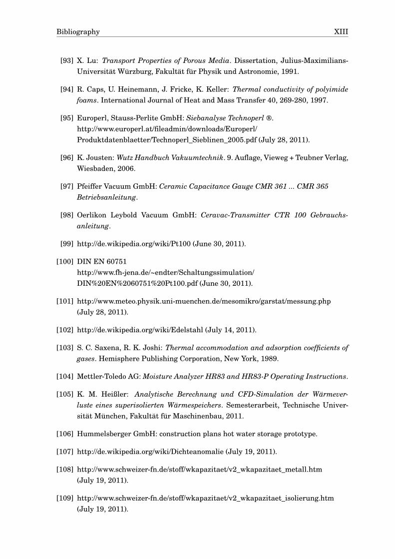
Bibliography XIII
[93] X. Lu: Transport Properties of Porous Media. Dissertation, Julius-Maximilians-Universität Würzburg, Fakultät für Physik und Astronomie, 1991.
[94] R. Caps, U. Heinemann, J. Fricke, K. Keller: Thermal conductivity of polyimidefoams. International Journal of Heat and Mass Transfer 40, 269-280, 1997.
[95] Europerl, Stauss-Perlite GmbH: Siebanalyse Technoperl ®.http://www.europerl.at/fileadmin/downloads/Europerl/Produktdatenblaetter/Technoperl_Sieblinen_2005.pdf (July 28, 2011).
[96] K. Jousten: Wutz Handbuch Vakuumtechnik. 9. Auflage, Vieweg + Teubner Verlag,Wiesbaden, 2006.
[97] Pfeiffer Vacuum GmbH: Ceramic Capacitance Gauge CMR 361 ... CMR 365Betriebsanleitung.
[98] Oerlikon Leybold Vacuum GmbH: Ceravac-Transmitter CTR 100 Gebrauchs-anleitung.
[99] http://de.wikipedia.org/wiki/Pt100 (June 30, 2011).
[100] DIN EN 60751http://www.fh-jena.de/~endter/Schaltungssimulation/DIN%20EN%2060751%20Pt100.pdf (June 30, 2011).
[101] http://www.meteo.physik.uni-muenchen.de/mesomikro/garstat/messung.php(July 28, 2011).
[102] http://de.wikipedia.org/wiki/Edelstahl (July 14, 2011).
[103] S. C. Saxena, R. K. Joshi: Thermal accommodation and adsorption coefficients ofgases. Hemisphere Publishing Corporation, New York, 1989.
[104] Mettler-Toledo AG: Moisture Analyzer HR83 and HR83-P Operating Instructions.
[105] K. M. Heißler: Analytische Berechnung und CFD-Simulation der Wärmever-luste eines superisolierten Wärmespeichers. Semesterarbeit, Technische Univer-sität München, Fakultät für Maschinenbau, 2011.
[106] Hummelsberger GmbH: construction plans hot water storage prototype.
[107] http://de.wikipedia.org/wiki/Dichteanomalie (July 19, 2011).
[108] http://www.schweizer-fn.de/stoff/wkapazitaet/v2_wkapazitaet_metall.htm(July 19, 2011).
[109] http://www.schweizer-fn.de/stoff/wkapazitaet/v2_wkapazitaet_isolierung.htm(July 19, 2011).

XIV Bibliography
[110] http://www.schweizer-fn.de/stoff/wleit_metall/v2_wleit_metall.htm(July 20, 2011).
[111] http://www.tommasinfondi.it/de/produkte/gewoelbte-gefaessboeden/typ-td/,325(July 20, 2011).
[112] http://www.weisstaler.de/web/1/produkte/boeden/kloepperboden.html(July 20, 2011).
[113] http://de.wikipedia.org/wiki/Kugelsegment (July 20, 2011).

XV
Acknowledgment
First, I would like to thank Prof. Dr. Rudolf Gross for his helpfulness and his willing-ness to supervise this master thesis, which has given me the opportunity to pursue mypersonal interests regarding the topic of the thesis.
My gratitude goes to Dr. Thomas Beikircher for supporting my work, providing helpfulinformation and discussing the details of heat transport and correlated topics, whichhas brought me a lot of knowledge and understanding.
Last but not least, I would like to thank my colleagues at ZAE BAYERN, especiallyDr. Frank Buttinger, Peter Kronthaler, Martin Heißler, Christopher Kaiser, PatrickWagner and Lukas Pospiech for their support and for the pleasant working atmosphere.