Physics-Based Optimal Controlsmocha-java.uccs.edu/ECE5720/ECE5720-Notes07.pdf · ECE5720,...

ECE5720: Battery Management and Control 7–1

Physics-Based Optimal Controls

7.1: Degradation as basis for power limits

■ We now approach the frontier of knowledge in battery management:

! The electronics aspects are important, but routine;

! State-of-charge is well defined, and established methods can beused to get good SOC estimates;

! Similarly, we have seen good methods to estimate resistance andtotal capacity of cells, yielding state-of-health estimates;

! Cell energy calculation is straightforward; and

! Several types of cell balancing—with varying complexities andspeed—can be implemented.

■ Improvements can yet be made to all of the above, but the presentstate of the art provides adequate BMS for many applications.

! Some questions regarding long-term efficacy of present BMS onaged battery packs;

! Other issues regarding power calculation, as described in thischapter.

■ “Using current electronics and knowledge it takes about two yearsand $250K to build a custom BMS” [Davide Andrea].

! Not trivial, but very doable.

Lecture notes prepared by Dr. Gregory L. Plett. Copyright c" 2013, 2015, Gregory L. Plett

ECE5720, Physics-Based Optimal Controls 7–2

More power!

■ The big pink elephant in the room that few people talk about is theway that power estimates are presently calculated.

■ The premise behind these methods is that voltage limits must neverbe violated.

■ But why? The real issue is cell degradation. The assumption is that:

! If voltage limits are violated, then the cell will degrade quickly;

! If limits are properly maintained, the cell will have a long andproductive and happy life.

■ But, in fact, voltage limits may be violated for a short time in somesituations without causing any faster aging.

■ And, “normal” voltages may also cause fast degradation in somesituations—particularly for an aged cell.

■ So, real issue is not cell voltage but rather rate of aging/degradation.

■ Cell power limits should really be calculated to more directly optimizea tradeoff between performance delivered by the cell and the rate ofincremental degradation experienced by the cell.

■ To be able to do this, we must be able to:

1. Model degradation mathematically, and2. Devise model-based optimized controls to calculate best tradeoff.

■ Some have suggested that if this is done perfectly, battery-pack sizesmay be reduced by up to 50 %, yet still deliver required performance.

! This is ample incentive to make a strong attempt.



Modeling cell degradation

■ We have seen that much is known about cell degradation qualitatively.

■ But, how about quantitatively? That is, can we make accuratemathematical models of all the degradation mechanisms?

■ We have seen that interactions between mechanisms are complex.Further, they are not presently well understood.

! Philosophy = “a blind man searching in a dark room for a black catthat isn’t there.” Are we on the same kind of futile search?

■ At this point, we don’t know. (That’s the nature of research!)

■ But, working in our favor is that we don’t need to model allmechanisms perfectly to have a useful result.

! For purposes of control, we don’t need to model any mechanismthat is not influenced by a variable that we have control over;

! If we model the most severe mechanisms reasonably well, then wehave a chance at designing controls that make a difference.

Literature that proposes models of degradation

■ The literature on degradation mechanism modeling is quite sparse.

■ Here, we look at two models: SEI formation/growth; lithium plating.



7.2: Full-order model of SEI formation and growth

■ Ramadass and colleagues have proposed a model that describes theformation and growth of an SEI layer on negative-electrode solidparticles during charging, that uses solvent reduction as the mainside reaction mechanism for degradation (Ramadass 2004).

■ Here, we build on that work to develop a simple incremental model ofSEI growth and associated capacity loss and resistance rise.1

■ The order-reduction method uses volume averaging to create analgebraic “0-D” model of the infinite-order PDE model.

■ This reduced-order model (ROM) of the SEI growth mechanism is afirst step toward creating a complete coupled reduced-order model ofall dominant cell degradation mechanisms, which then could be usedin an optimal control scheme.

Original model

■ Changes at the electrode/electrolyte interface due to side reactions atthe negative electrode are considered to be one of the primarycauses of cell aging.

■ There are a large number of reduction reactions that can lead to thedeposition of solid SEI products on the electrode surface, and theseare less well understood, being very dependent upon the compositionof the electrolyte solution.

1 Adapted from, Randall, A.V., Perkins, R.D., Zhou, X., Plett, G.L., “Controls OrientedReduced Order Modeling of SEI Layer Growth,” Journal of Power Sources, Vol. 209,July 2012, pp. 282–288.



■ Ramadass makes general assumptions that the side reaction isconsidered to be a consumption of the solvent species and lithiumions, which will form compounds such as Li2CO3, LiF, Li2O, and soforth, depending on the nature of the solvent.

■ There is significant porosity in the film, and this makes it reasonableto assume that the SEI layer continues to grow as the solvent diffusesthrough the layer during charge.

■ The assumption of the ongoing formation of the SEI layer is alsosupported by the research of Aurbach and colleagues (1999), whopropose that the intercalation of lithium into the graphite negativeelectrode leads to increase in the lattice volume, which in turnstretches the SEI layer, causing it to fracture and to expose more ofthe active material to the electrolyte, fueling the side reaction, andcontributing to SEI formation.

■ Ramadass’ model assumes:

1. The main side reaction is due to the reduction of an organicsolvent, expressed as S C 2LiC C 2e# ! P, where “S” refers to thesolvent and “P” to the product formed in the side reaction.

2. The reaction occurs only during charging of the cell.3. The products formed are a mixture of different species, resulting in

averaged mass and density constants used in the later equationdescribing the formation and growth of the SEI film.

4. The side reaction is assumed to be irreversible and U refs is chosen

to be 0:4 V versus Li=LiC.5. The initial resistance of the SEI layer developed during cell

formation is 0:01 !m2.



6. There is no overcharge reaction considered (i.e., lithium plating isnot modeled).

■ We have somewhat relaxed assumption 2, allowing side reactions tooccur during rest intervals also (and even during discharge).

■ The SEI growth model is tightly coupled with a Newman-stylephysics-based model of ideal-cell dynamics.

■ For the negative electrode, the local molar flux jtotal is given by a sumof the intercalation flux j and the side reaction flux js,

jtotal D j C js,

where j is computed via the Butler–Volmer electrochemical kineticexpression

j D i0

F

!exp

"˛aF

RT"

## exp

"#˛cF

RT"

#$,

which is driven by the overpotential

" D #s # #e # U refn # FRfilmjtotal,

where i0 [A m#2] is the exchange current density and U refn is the

equilibrium potential in the negative electrode, evaluated as a functionof the solid-phase concentration at the surface of the particle.

■ The kinetics of the side reaction are described using a Tafel equation,which assume that the side reaction is considered irreversible,

js D #i0;s

Fexp

"#˛sF

RT"s

#,

and the side reaction overpotential is described as

"s D #s # #e # U refs # FRfilmjtotal.



■ Once the side reaction flux, js, has been calculated, the change inthe film thickness ıfilm during charging can be calculated by

@ıfilm

@tD #MP

$Pjs,

where MP [kg mol#1] is the average molecular weight of theconstituent compounds of the SEI layer and $P [kg m#3] is theaverage density of the constituent compounds.

■ This allows the overall film resistance to be calculated as

Rfilm D RSEI C ıfilm=%P ,

where RSEI is the initial film resistance that is produced during theformation period of the cell, and %P [S m#1] is the conductivity of thefilm.

■ In addition to the resistance change, there is a capacity loss causedby the side reaction current during charge, leading to capacitychanging via the relationship

@Q

@tDZ Ln

0

anAFjs dx.



7.3: Simplifying the model

■ To effect an optimal control strategy, the battery management systemmust be able to calculate the side reaction flux js very quickly andaccurately.

■ Solving the coupled PDE equations described above (plus thephysics-based ideal-cell model) is too complicated for such a process.

■ The js model needs to be much faster and simpler. In this section, wepresent a simpler incremental model for calculating js, Rfilm, and Q.

■ To create a volume-averaged 0-D reduced-order model, threeadditional assumptions are made:

1. The cell is always in a quasi-equilibrium state, allowing theexchange current density i0 to be calculated from the cell SOCalone, neglecting local variations in electrolyte and solid surfaceconcentration. The estimated value of js then corresponds to asuddenly applied current pulse iapp.t/, which is constant over sometime interval &t .

2. The intercalation and the side-reaction fluxes are uniform over thenegative electrode. This allows us to state that the total reactionflux jtotal is related to the applied cell current iapp by the followingrelationship:

jtotal D iapp

anF Voln,

where the volume of the active material is described byVoln D LnA.

3. The anodic and cathodic charge-transfer coefficients are equal(˛a D ˛c D 0:5/.



■ From the above assumptions, an incremental degradation model canbe formulated as follows. First, at any point in time, the lithiation stateof the negative electrode is calculated as

'n D 'n;min C SOCcell .'n;max # 'n;min/ ,

where:

! 'n;max and 'n;min are the stoichiometric limits of negative-electrodelithiation (i.e., the value of ' in Li'C6 when the cell is fully chargedand discharged, respectively).

! SOCcell is a value between zero and one, which indicates the cellstate-of-charge.

■ Then U refn is calculated from 'n for the electrode materials being used.

■ We will ultimately iterate to find js. We can initialize its value to zeroand calculate the intercalation flux:

j D jtotal # js

D iapp

anF Voln# js.

■ From j and assumption 3,

j D i0

F

!exp

"F

2RT"

## exp

"# F

2RT"

#$

D 2i0

Fsinh

"F

2RT"

#

" D 2RT

Fasinh

"Fj

2i0

#.

■ Then, we note the similarity between the expressions for " and "s tofind:



" D #s # #e # U refn # FRfilmjtotal

"s D #s # #e # U refs # FRfilmjtotal

D " C U refn # U ref

s

D 2RT

Fasinh

"Fj

2i0

#C U ref

n # U refs .

■ The film resistance cancels from the calculation. We can nowcalculate an updated estimate of the side-reaction flux as

js D #i0;s

Fexp

" #F

2RT"s

#.

■ In total, we have the reduced-order model

js D #i0;s

Fexp

#F

2RT

2RT

Fasinh

"Fj

2i0

#C U ref

n # U refs

!!

D #i0;s

Fexp

#F

2RT

2RT

Fasinh

0

B@F%

iappanF Voln

# js

&

2i0

1

CAC U refn # U ref

s

!!

D #i0;s

Fexp

F'U ref

s # U refn

(

2RT

!exp

asinh

#iappanVoln

C Fjs

2i0

!!.

■ We’ll see how to solve this equation for js shortly.

■ Once we have solved for js it can then be incorporated intoincremental equations for film resistance and capacity loss.

■ It is assumed that js is constant over some small time interval &t , andis denoted as js;k for the kth interval.

■ We can convert the continuous-time film thickness relationship todiscrete time as:



@ıfilm

@tD #MP

$P

js

ıfilm;k D ıfilm;k#1 # MP &t

$P

js;k#1,

noting that the sign of js is negative.

■ This result can be used to calculate the film resistance as

Rfilm D RSEI C ıfilm=%P

Rfilm;k D Rfilm;k#1 # MP &t

$P %P

js;k#1.

■ Similarly, we can discretize the capacity equation

@Q

@tDZ Ln

0

anAFjs dx

Qk D Qk#1 C .anAFLn&t/ js;k#1.

■ In summary, the proposed reduced-order model (ROM) equationsare:

'n D 'n;min C SOCcell .'n;max # 'n;min/

js;k D #i0;s

Fexp

F'U ref

s # U refn

(

2RT

!exp

asinh

#iappanVoln

C Fjs;k

2i0

!!,


$P %P

js;k#1




7.4: Simplifying the calculation

■ As it is written now, js;k is an implicit calculation

js;k D #i0;s

Fexp

F'U ref

s # U refn

(

2RT

!exp

asinh

#iappanVoln

C Fjs;k

2i0

!!.

■ One solution methodology would be to use iteration:

1. Guess a value for js;k (e.g., zero),2. Plug in to RHS of relationship; calculate LHS as new value for js;k,3. Repeat step 2 until no significant change in js;k.

■ This method actually works pretty well, and we can arrive at asolution in fewer than 10 iterations.

■ However, there is also a closed-form solution for js;k (not obvious).

■ First, let’s simplify notation:

js;k D #i0;s

Fexp

F'U ref

s # U refn

(

2RT

!

„ ƒ‚ …A

exp

0

BB@asinh

0

BB@#iapp

2ani0Voln„ ƒ‚ …B

C F

2i0„ƒ‚…C

js;k

1

CCA

1

CCA

D A exp .asinh .B C Cjs;k// .

■ Note that A < 0 and C > 0 always.

■ Also note that the value of A can be stored in a lookup table versus'n, so is not difficult to calculate in real time.

■ A useful identity for simplifying this further is:

exp.asinh.x// D x Cp

x2 C 1.

■ So, we can write



js;k D A

!.B C Cjs;k/ C

q.B C Cjs;k/2 C 1

$

js;k

A# B # Cjs;k D

q.B C Cjs;k/2 C 1

js;k.1 # CA/ # AB D A

q.B C Cjs;k/2 C 1

.js;k.1 # CA/ # AB/2 D A2 .B C Cjs;k/2 C A2

0 D A2 .B C Cjs;k/2 C A2 # .js;k.1 # CA/ # AB/2

D A2'B2 C 2BCjs;k C C 2j 2

s;k

(C A2

#'j 2

s;k.1 # CA/2 # 2AB.1 # CA/js;k C A2B2(

.

■ Collecting like terms

0 D'A2C 2 # .1 # CA/2

(j 2

s;k C'2A2BC C 2AB.1 # CA/

(js;k

C'A2B2 C A2 # A2B2

(.

■ Note that .1 # CA/2 D 1 # 2CA C A2C 2, so this simplifies,

0 D .2CA # 1/ j 2s;k C .2AB/ js;k C

'A2(

.

■ Key point: This is a quadratic, so we can easily solve for the root(s)using the quadratic formula:

js;k D #2AB ˙p

4A2B2 # 4A2.2CA # 1/

2.2CA # 1/

D AB ˙ Ap

B2 C .1 # 2CA/

.1 # 2CA/.

■ But, which root to use? The Routh test gives us some guidance:



j 2s;k 2CA # 1, A2

js;k 2AB

1 A2

■ Since 2CA # 1 < 0 and A2 > 0, we are guaranteed two sign changes,which means that this equation always has exactly one positive realroot and one negative real root.

■ Physically, we know that js;k < 0 (because A < 0), so we want to takethe smaller root of the quadratic solution.

■ So, because A < 0,

js;k D AB C Ap

B2 C .1 # 2CA/

.1 # 2CA/.



7.5: Comparing the models

■ The validity of this reduced-order model depends first on the accuracyof the underlying partial differential equation model, which weassume here to be exact.

■ It then depends on how closely the reduced-order approximation of js

matches the exact calculation of js.

■ To compare the PDE and reduced-order models, we conducted aseries of simulations.

! In each simulation, the cell was initially at rest.

! A sudden pulse of current was then applied, and the instantaneousresulting js from the PDE model was compared to the computed js

from the ROM.

■ To simulate the PDE model, we used COMSOL Multiphysics 3.5acoupled with a MATLAB script to cycle through the series ofsimulations and analyze results.

! Specifically, each simulation comprised a 1 s time interval, wherethe cell current iapp was modeled as a Heaviside step function,which was applied half-way through the interval.

! We found that the initial rest interval facilitated convergence of thesolution by allowing the PDE solver to adjust its initial conditionsbefore applying the step current.

■ The simulation cell parameters that we used are listed in theappendix. In particular, the cell had a 1:8 Ah capacity.

■ For the full-order PDE simulations:



! Applied current was varied from 0 A to 5:4 A in steps of 0:1 A;

! Initial cell SOC was varied from 0 % to 100 % in steps of 2 %; and

! Temperature was varied from #35 ıC to 45 ıC in steps of 20 ıC.

■ For the reduced-order simulations, which run much more quickly:

! Applied current was varied from 0 A to 5:4 A in steps of 0:05 A;

! Initial cell SOC was varied from 0 % to 100 % in steps of 1 %; and

! Temperature was varied from #35 ıC to 45 ıC in steps of 10 ıC.

■ As one point of comparison, the set of 14 025 full-order PDEsimulations took more than eight days to complete on an Intel i7processor, while the set of 112 200 ROM simulations took a total ofabout 2.6 seconds to complete on the same machine.

■ The speedup, on a per-simulation basis, is more than 2 000 000 W 1.This is the primary advantage of the ROM over the PDE model.

■ The figure below-left shows room-temperature side-reaction flux js ascomputed by the reduced-order model (which we now denote asjs;ROM).

■ The figure below-right shows a compilation of js;ROM over a range oftemperatures. We see two trends that match experience: degradationis worst at high SOC and high charge rates.



■ The figure to the right showsresults of one PDE simulation.

■ This example was conducted at25 ıC, 50 % SOC, and byapplying a 1C charge pulse att D 0:5 s.

■ The figure shows the raw outputof the simulation, as comparedto the ROM.

0 0.2 0.4 0.6 0.8 1−0.26

−0.255

−0.25

−0.245

−0.24

−0.235

−0.23

Time (s)

J s (mA

cm−3

)

Comparing ROM to PDE solutions

PDEROM

■ Both the PDE and ROM solutions have a non-zero negative sidereaction flux js even when the cell is at rest.

■ This is due to the fact that we have relaxed assumption 2 of the SEIgrowth model to also allow for the side reaction when current in theexternal circuit is zero.

■ The figure shows that the ROM matches both the rest SEIside-reaction rate and the charge-pulse SEI side-reaction rate.

■ Plotted on the same scale, the full PDE solution results areindistinguishable from the ROM results. So, for comparison purposes,



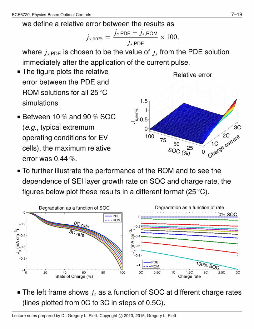
we define a relative error between the results as

js;err% D js;PDE # js;ROM

js;PDE$ 100,

where js;PDE is chosen to be the value of js from the PDE solutionimmediately after the application of the current pulse.

■ The figure plots the relativeerror between the PDE andROM solutions for all 25 ıCsimulations.

■ Between 10 % and 90 % SOC(e.g., typical extremumoperating conditions for EVcells), the maximum relativeerror was 0:44 %.

1C2C

3C

02550751000

0.51

1.5

Charge current

Relative error

SOC (%)

J s,er

r%

■ To further illustrate the performance of the ROM and to see thedependence of SEI layer growth rate on SOC and charge rate, thefigures below plot these results in a different format (25 ıC).

0 20 40 60 80 100−1

−0.8

−0.6

−0.4

−0.2

0

State of Charge (%)

J s (mA

cm−3

)

Degradation as a function of SOC

0C rate3C rate

PDEROM

0C 0.5C 1C 1.5C 2C 2.5C 3C

−1

−0.8

−0.6

−0.4

−0.2

0

Charge rate

J s (mA

cm−3

)

Degradation as a function of rate

0% SOC

100% SOCPDEROM

■ The left frame shows js as a function of SOC at different charge rates(lines plotted from 0C to 3C in steps of 0.5C).



■ The right frame shows js as a function of charge rate at differentSOCs (plotted from 0 % SOC to 100 % SOC in steps of 10 % SOC).

■ In all plots, the corrected PDE result is drawn as a solid line, and theROM result is drawn as a dashed line. In most cases, it is impossibleto visually distinguish between the PDE and ROM results.

■ The figures below show additional effects on relative error. First, wesee how error varies with temperature.

■ The ROM predictions are bestat high temperatures, and lessgood at low temperatures.

! Worst-case js;err% in the 10 %to 90 % SOC range variesfrom 0:41 % at 45 ıC to0:55 % at #35 ıC. 0C

1C2C

3C

025

5075

1000

0.5

1

1.5

Charge current

Effect of temperature on results

SOC (%)

J s,er

r%

−35°C

−15°C

5°C

25°C

45°C

■ Next, we investigate the effect of &t on the results. Instead ofselecting the value for js;PDE immediately after the application of thecurrent pulse, js;PDE is now selected to be the PDE solution 0:5 sseconds after the application of the current pulse, at the t D 1 s point.

■ The relative error is once againworst at low temperatures andlow values of SOC (where theabsolute amount of degradationis small).

0C1C

2C3C

025

5075

1000

5

10

Charge current

Effect of 0.5s ∆t on results

SOC (%)

J s,er

r%

−35°C

−15°C

5°C

25°C

45°C



■ Relative errors over 10 % are observed in some cases, but in theranges of SOC most important for control, where SOC is greater than25 %, the worst-case js;err% is far less, varying from 0:85 % at 45 ıC to1:04 % at #35 ıC.

■ The figure to the rightinvestigates the effect of aprolonged constant-currentcharge at a 1C rate, as might beexperienced when a cell isbeing charged.

0 0.2 0.4 0.6 0.8 1−1

−0.8

−0.6

−0.4

−0.2

0

Dimensionless distance across anodeJ s (m

A cm

−3)

PDE and ROM solutions over extended period

100 s1000 s2000 s

3000 s1D PDE computation of JsAvg. over width of PDE computation of JsROM computation of average Js

■ The PDE is simulated for 3 000 s, starting with the cell at rest at 10 %SOC, and 1D profiles of js.x/ across the negative electrode areplotted at time steps 100 s; 1 000 s, 2 000 s, and 3 000 s.

■ Overlaid on the plot are the average js values predicted by the ROMat that SOC level, and the actual averaged js values (averaged overthe 1D electrode) from the PDE solution.

■ In the ROM simulation, the SOC is updated on a second-by-secondbasis to achieve the present SOC at every point, which is used tocompute the value of js using the method explained herein.

■ We see that even over prolonged constant-current charge profiles,the ROM is accurate, indicating that assumption 1 of ROM is areasonable assumption to make.



7.6: Lithium deposition on overcharge

■ The success of the preceding ROM to predict the performance of aTafel equation leads us to expect it will work well for other similaraging mechanisms (e.g., Darling and Newman, 1998).

■ The PDE model of lithium deposition on overcharge by Arora et al.,however, does not use a Tafel equation.

! Instead, it uses a modified Butler–Volmer equation.

■ Here, we address creation of a ROM of lithium deposition onovercharge.2

! It does not work as well as the SEI ROM, especially for prolongedcharging events.

! It is probably better suited for predicting degradation in an HEVscenario, with random charges.

! We’re working on another method right now, that we think will workbetter, but it isn’t ready for public consumption as yet.

■ Lithium deposition/plating is not usually considered a dominantdegradation mechanism, because the cell terminal voltage limits aredesigned to avoid conditions that would be conducive to plating.

! However (especially at cold temperatures), the terminal voltagesare poor indicators of internal cell potentials,

! Plating can still happen, and when it does, there is immediatesevere capacity loss.

2 Adapted from, Perkins, R.D., Randall, A.V., Zhou, X., Plett, G.L., “Controls OrientedReduced Order Modeling of Lithium Deposition on Overcharge,” Journal of PowerSources, Vol. 209, July 2012, pp. 318–325.



■ So, modeling lithium deposition is very important to be able to deviseoptimized controls to minimize aging.

■ Overcharge manifests first as a metallic lithium deposit on the surfaceof the negative electrode solid particles during charge, predominantlynear the separator.

■ Subsequently, the lithium can and does further combine withelectrolyte material to form other compounds such as Li2O, LiF,Li2CO3, and polyolefins.

■ The nature of the final product is not our major concern; rather, theissue is that lithium is irreversibly lost.

■ This phenomenon is an unintended side reaction that can lead tosevere capacity fade, electrolyte degradation, possible safety hazard.

Physics-based model of overcharge

■ This work is based on a physics-based model proposed by Arora etal. (1999).

■ Our goal is to create a high-fidelity reduced-order model of this PDEdegradation model; therefore, we adopt the same assumptions asthey, which were:

1. The main side reaction is expressed as LiC C e# ! Li.s/, whichoccurs at U ref

s D 0 V versus Li/LiC during an overcharge event. Thislithium metal is expected to form first near the electrode-separatorboundary where the surface overpotential is greatest.

2. Lithium metal deposited on the negative electrode reacts quicklywith solvent or salt molecules in the vicinity, yielding Li2CO3, LiF, or



other insoluble products. A thin film of these products protects thesolid lithium from reacting with the electrolyte. Solid lithium can stilldissolve during discharge, but once lithium is consumed in ainsoluble product, it is permanently lost.

3. The insoluble products formed are a mixture of different species,resulting in averaged mass and density constants used in a laterequation describing the formation and growth of a resistive film.

4. Only the overcharge reaction is considered (e.g., SEI film growthand other degradation mechanisms are not modeled).

■ The overcharge model of Arora is tightly coupled with a “pseudotwo-dimensional” Newman-style porous-electrode style model ofideal-cell dynamics.

■ In the ideal cell, intercalation flux j.x; t/ is expressed as theButler–Volmer equation,

j.x; t/ D i0

F

!exp

"˛a;nF

RT".x; t/

## exp

"#˛c;nF

RT".x; t/

#$

which is driven by the overpotential

".x; t/ D #s.x; t/ # #e.x; t/ # U refn # FRfilmj.x; t/,

where i0 is the exchange current density,

i0 D kn

'cmax

s;n # cs;n

(˛a;n .cs;n/˛c;n .ce/˛a;n ,

and U refn is the equilibrium potential which is evaluated as a function

of the solid phase concentration at the surface of the particle.

■ Arora expresses the side-reaction flux js (i.e., the rate of irreversiblelithium loss due to lithium plating) as



js.x; t/ D min

0;

io;s

F

"exp

˛a;sF

RT"s.x; t/

!# exp

# ˛c;sF

RT"s.x; t/

!#!,

where ˛a;s ¤ ˛c;s in general,

"s.x; t/ D #s.x; t/ # #e.x; t/ # U refs # FRfilmjs.x; t/,

and where the side-reaction exchange current densityi0;s D kn;s.ce/

˛a;s.

■ Side reaction is semi-irreversible in the sense that it includes ananodic rate term, but doesn’t allow overall positive side-reaction flux.

■ The side reaction occurs only at spatial locations in the negativeelectrode where "s.x; t/ < 0.

■ This is enforced in the js equation by the “min” function, which setsjs.x; t/ D 0 for values of x where "s.x; t/ % 0, but to the valuecomputed by the Butler–Volmer equation when "s.x; t/ < 0.

■ A typical scenario is plotted in thefigure, where "s.x; t/ is sketchedacross the electrode width.

■ In this example, plating will occur in theinterval from x D x0 to x D Ln.

■ Note that this illustration shows that the cell can be quite far awayfrom 100 % state-of-charge and still have plating occur near theseparator if a large enough charge-current pulse is applied to thecell’s terminals.

! The state-of-charge is only one variable of importance—ultimately,the local overpotential determines whether plating occurs.



■ So, our first goal will be to solve for js. Then, once we have solved forjs, it can then be incorporated into incremental equations for filmresistance and capacity loss.

■ We assume that js is constant over some small time interval &t , anddenote it as js;k for the kth interval.

■ We can convert the continuous-time film thickness relationship todiscrete time as:

@ıfilm

@tD #MP

$Pjs

ıfilm;k D ıfilm;k#1 # MP &t

$Pjs;k#1,

where MP and $P are the average molecular weight and density oflithium and products, noting that the sign of js is negative.

■ This result can be used to calculate the film resistance as

Rfilm D RSEI C ıfilm=%P


$P %Pjs;k#1.

■ Similarly, we can discretize the capacity equation

@Q

@tDZ Ln

0

anAFjs dx




7.7: Simulation and results

■ A reduced-order model is derived in the aforementioned paper.

■ The validity of this reduced-order model depends first on the accuracyof the underlying partial differential equation model, which weassume here to be exact.

■ It then depends on how closely the reduced-order approximation of Njs

matches the exact calculation of Njs. In this section, results from boththe full and reduced-order models for Njs are compared.

■ To compare the PDE and reduced-order models, we conducted aseries of simulations.

! In each simulation, the cell was initially at rest.

! A sudden pulse of current was then applied, and the resulting Njs

from the PDE model, averaged over a one-second intervalsubsequent to the pulse, was compared to the computed Njs fromthe ROM.

■ To simulate the PDE model, we used COMSOL Multiphysics 3.5acoupled with a MATLAB script to cycle through the series ofsimulations and analyze results.

■ Specifically, each simulation comprised a 1:2 s time interval, wherethe cell current iapp was modeled as a step function, which wasapplied at t D 0:2 s.

■ We found that the initial rest interval facilitated convergence of thesolution by allowing the PDE solver to adjust its initial conditionsbefore applying the step current.



■ The cell parameters that we used in the simulations match thoseused in Arora and are listed in the appendix.

! The applied current was varied between 0C and 3C in incrementsof C/33;

! The initial cell SOC was varied between 0 % and 100 % in steps of1 %, and

! Temperature was held constant at 25 ıC.

■ We found that the adjustable tuning factor ˇ D 1:7 worked well (thisimplies the change in electrolyte concentration near the separatorchanges nearly twice as quickly as it does near the current collector).

■ A total of 10 100 simulations were run.

! As one point of comparison, the set of full-order PDE simulationstook approximately 12 hours to complete, utilizing an average ofthree cores, on an Intel i7 processor, while

! The set ROM simulations took approximately 21 seconds tocomplete, utilizing an average of one core on the same machine.

! The speedup, on a per-simulation per-core basis, is more than5 000 W 1. This is the primary advantage of the ROM over the PDEmodel.

■ Lithium plating occurs when the side-reaction overpotential isnegative ."s < 0/.



■ The figure illustrates theside-reaction overpotentialacross the negative electrodefor this cell model, where x D 0

is adjacent to thecurrent-collector and x D 85 (mis adjacent to the separator,immediately following the onsetof a charge current pulse.

0 10 20 30 40 50 60 70 80−30

−20

−10

0

10

20

Anode location (µm)

Ove

rpot

entia

l ηs (m

V)

Overpotential predictions at 90% SOC, 2.0C rate

PDEROM

■ From the PDE result, we expect lithium deposit to occur betweenabout x D 42 (m and x D 85 (m. From the ROM, we expect lithiumdeposit to occur between x0 D 49 (m and x D 85 (m.

■ The figure to the right shows theresulting rate of lithiumdeposition for the PDE andROM solutions.

■ The time-average depositionrate of the ROM is somewhathigher than the time-averagedeposition rate of the PDE overthe 1 s interval.

−0.2 0 0.2 0.4 0.6 0.8 1−250

−200

−150

−100

−50

0

Time (s)

O

verc

harg

e ra

te j s (m

A cm

−3)

Overcharge predictions at 90% SOC, 2.0C rate

PDEROM

■ The figures below illustrate the predicted overcharge rates over allscenarios for the PDE and the ROM solutions.



■ As expected, deposition is worse at high SOC and high charge rates.The PDE and ROM solutions generally agree very well, with greatestmismatch at high charge rates.

■ The figures below show a different view of the results.

! Cross sections through both the PDE and ROM solution spacesare plotted and compared.

0 20 40 60 80 100−700

−600

−500

−400

−300

−200

−100

0

SOC (%)

Ove

rcha

rge

j s (mA

cm −3

)

Instantaneous degradation rate as function of SOC

Charge at 1C rate

Charge at 2C rate

Charge at 3C ratePDEROM

0C 1C 2C 3C−700

−600

−500

−400

−300

−200

−100

0

Charge current

Ove

rcha

rge

j s (mA

cm−3

)

Instantaneous degradation rate as function of current

SOC = 60%SOC = 70%

SOC = 80%SOC = 90%

SOC = 100%PDEROM

■ The left figure shows how the two methods compare where each pairof lines represents a specific charge rate.



! As noted before, but perhaps more clearly seen here, thedifference between the PDE and ROM solutions are greatest athigh charge rates.

■ The right figure shows how the two methods compare where eachpair of lines represents a specific initial SOC.

! The difference is greatest at moderate SOC levels.

■ Finally, the figures below illustrate the error between the PDE andROM solutions in two ways.

Neither PDE nor ROMpredict overcharge inthis region

Both PDE and ROMpredict overcharge in

this region

Charge current

SOC

(%)

Regions where models predict overcharge

0C 1C 2C 3C0

25

50

75

100

■ The left frame shows the regions where the two methods agree onwhether lithium deposition will occur, and the region where theydisagree.

! The region of disagreement is the very narrow sliver at around2.4C and 25% SOC, where the ROM predicts overcharge but thePDE does not.

! Otherwise, the boundaries are identical.



■ The right frame shows the error between the solutions, calculated asNjs;ROM # Njs;PDE. The maximum error is approximately 65 mA cm#2

(relative error on the order of 10 %).

■ For the purpose of control system design, the results of the left frameare the most important.

■ Since lithium deposition is such a severe degradation mechanism, acharging control scheme should avoid ever commanding a controlaction that would cause any lithium deposition to occur.

■ A time-optimal charger, based only on the PDE model of lithiumdeposition, would select charge pulse current to follow the uppercontour in the left frame.

! This allows the maximum charge rate at any point in time, whilecausing no lithium plating.

■ In comparison, a time-optimal charger, based only on the ROM modelof lithium deposition, would select charge pulse current to follow thelower contour in the figure.

! This will result in somewhat slower charging.

! But, because the ROM over-predicts the amount of lithiumdeposition, it will also result in a charging scheme that isconservative, which is a beneficial feature.

■ We conducted additional simulations to investigate the effect of pulselength &t in assumption 1.

■ That is, how long can the charge pulse be before the full-order PDEmodel and the reduced order model results are significantly different?



■ We found that pulse lengths less than 10 s are generally wellmatched, but pulse lengths much greater than 10 s can givesignificant PDE versus ROM mismatch.

■ For long pulse durations, the quasi-static nature of assumption 1 isviolated, and an a significant offset is noted in actual time-varying #e

versus the at-rest #e, moving the crossover point of "s.x; t/.

■ This causes the ROM to under-predict the value of lithium platingcomputed by the PDE.

■ For this reason, we propose that the ROM is of most value forcomputing current limits in dynamic applications such ashybrid-electric vehicles, where a bias in #e cannot develop due to therandom nature of power demand, but is of less value for controllingfull charges, such as for electric vehicle applications.

■ We make one final comment regarding efficiency.

! The speedup of ROM vs. PDE can be much greater than 5 000 W 1 ifROM solutions are pre-computed and stored in a table.

! Then, “computing” any value of Njs;ROM would be nearlyinstantaneous, via table lookup.

■ We note that the ROM solution changes as the film resistancechanges, but the film resistance changes very slowly.

■ The entire table might be updated by the battery management systemonce per operational period (e.g., once per day), and then utilizedthroughout that operational period for significant performance gains.



7.8: Optimized controls for power estimation

■ We’ve now seen that there are quite a few causes of cell degradation,and an attempt at modeling two of the more significant mechanisms.

■ Much more work remains to be done in this area, first by materialsscientists, then by controls engineers.

■ But, how to use these models to compute power to slow aging? Welook at a few methods next.

■ We have seen that none of the cell degradation mechanisms are tieddirectly to the cell terminal voltage, but rather to internal stress factors.

■ Therefore, assuming that degradation mechanisms can be wellmodeled, it makes more sense to compute power limits based onpredicted capacity loss and/or impedance rise than on voltage limits.

■ Clearly, there’s a lot of work to do before this is practical, but thepotential benefits are worth it.

■ The next sections of notes very briefly introduce some optimizationmethods that might be used with the physics-based degradationmechanisms to compute better power limits.

Two problems

■ There are (at least) two controls problems to consider.3

■ For EV/E-REV/PHEV, the battery pack is charged from an externalsource:

3 A third, well beyond our scope here: Considering xEV as storage units for the “smartgrid,” when does it make sense to “lend” energy to the grid? What should be the rentalfee charged for allowing energy to be borrowed?



! What is the optimum charge profile?

! Can we “fast charge”?

! For a fixed charge period, what is the best strategy?

■ For all xEV, while the car is being driven,

! What is the maximum charge power that can be maintained overthe next &T seconds?

! What is the maximum discharge power that can be maintainedover the next &T seconds?

■ Different kinds of optimized controls may be better for these twoproblems.



7.9: Plug-in charging

■ The plug-in charging problem lends itself well to being solved by anonlinear programming method.

! One example is the sequential quadratic programming algorithm,implemented in MATLAB as fmincon.m.

■ Nonlinear programming is a generic optimization method thatattempts to find solutions to problems that can be posed in theframework:

x& D arg min f .x/; such that

8<̂

:̂

c.x/ ' 0 Ax ' b

ceq.x/ D 0 Aeqx D beq

lb ' x x ' ub,

where f .x/ is a function that we wish to minimize by choosingoptimum input vector x& such that

! Nonlinear inequality constraint vector function c.x/ ' 0 is satisfied,

! Nonlinear equality constraint vector function ceq.x/ D 0 is satisfied,

! Linear inequality constraint vector function Ax ' b is satisfied,

! Linear equality constraint vector function Aeqx D beq is satisfied,

! Bounds lb ' x ' ub for all entries in vector x are satisfied

for user-specified f .x/, c.x/, ceq.x/, A, b, Aeq, beq, lb, and ub.

■ We will choose x to be a vector of cell applied current versus time,f .x/ to be some estimate of the cell degradation that would becaused by that applied current, and the other functions and matricesto make the problem work.



■ For example, we might want to find

i& D arg minK#1X

kD0

#Js .ik; ´k; Tk/

such that

8<̂

:̂

´min ' ´k ' ´max

´K D énd

#Imax ' ik ' Imax

and ´k D ´0 #X

j <k

ij &t=Q.

■ This states that we want to minimize capacity loss that would beexperienced by a cell if we were to start at SOC ´0 and end at SOCénd over a period of K sampling intervals, where current is limitedbetween ˙Imax, and SOC is limited between ´min and ´max and thestandard SOC equation holds.

■ It takes a little work to recast this problem in the right framework, butit’s not too bad.

■ First, consider the SOC equation. We can write it in vector form as:2

66664

´1

´2:::

´K

3

77775D

2

66664

1

1:::

1

3

77775

„ƒ‚…C V

´0 # &t

Q

2

66664

1 0 0 0 ( ( ( 0

1 1 0 0 ( ( ( 0::: ::: ::: ::: : : : :::

1 1 1 1 ( ( ( 1

3

77775

„ ƒ‚ …LT

2

66664

i0

i1:::

iK#1

3

77775

„ ƒ‚ …x

.

! Notice that the matrix LT is lower-triangular.

■ Using this formulation, we can write an equation for the ´K constraint

´K D ´0 # &t

Q

h1 1 1 ( ( ( 1

ix D énd,



or, in the prescribed format for fmincon.m,h

1 1 1 ( ( ( 1i

„ ƒ‚ …Aeq

x D Q

&t.´0 # ´end/

„ ƒ‚ …beq

.

■ The limit ´min ' ´k can be written as2

66664

1

1:::

1

3

77775´min '

2

66664

1

1:::

1

3

77775

„ƒ‚…CV

´0 # &t

Q

2

66664

1 0 0 0 ( ( ( 0

1 1 0 0 ( ( ( 0::: ::: ::: ::: : : : :::

1 1 1 1 ( ( ( 1

3

77775

„ ƒ‚ …LT

2

66664

i0

i1:::

iK#1

3

77775

„ ƒ‚ …x

.CV/.´min # ´0/ ' #&t

Q.LT/ x

.LT/ x ' Q

&t.CV/.´0 # ´min/.

■ Similarly, ´k ' ´max can be written as

#.LT/x ' Q

&t.CV/.´max # ´0/.

■ Putting the last two constraints together gives"LT

#LT

#

„ ƒ‚ …A

x ' Q

&t

".CV/.´0 # ´min/

.CV/.´max # ´0/

#

„ ƒ‚ …b

.

■ The constraints on input current can be satisfied by setting

lb D #Imax.CV/; and ub D Imax.CV/.

■ Then, all that’s left is to specify the cost function f .x/. (There are nononlinear constraints in this problem.)

■ Given what we’ve seen so far, we might consider js to represent theSEI growth model, or the overcharge model, or the sum of both.



7.10: Fast-charge example

■ We designed optimized controllers to investigate charging strategiesusing the degradation models generated to date.

■ In the first controls scenarios, the cell was initially at a SOC valuebetween 10 % and 90 %, and the charger was required to optimallycharge the cell to 90 % over a period of two hours.

■ SOC was not allowed outside the range of 10 % to 90 %, but currentwas unconstrained.

■ We first looked at using only the SEI-growth degradation model in thecontrol strategy:

0 20 40 60 80 100 120

−2C

0

2C

4C

6C

Time (min)

Rate

Strategy for SEI cost function

z0 = 90%z0 = 70%z0 = 50%z0 = 30%z0 = 10%

0 20 40 60 80 100 1200

20

40

60

80

100

Time (min)

SOC

(%)


z0 = 90%z0 = 70%z0 = 50%z0 = 30%z0 = 10%

■ The optimum charging strategy for this model is to quickly dischargethe cell to the minimum SOC, wait “as long as possible” and thenquickly charge the cell to the desired SOC.

■ The cost of discharging plus charging turns out to be less than thecost of maintaining a high SOC for an extended period of time(!)

■ We then looked at using the SEI plus the overcharge cost functionsadded together:



0 20 40 60 80 100 120

−2C

0

2C

4C

6C

Time (min)

Rate

Strategy for SEI/ovchg cost function

z0 = 90%z0 = 70%z0 = 50%z0 = 30%z0 = 10%

0 20 40 60 80 100 1200

20

40

60

80

100

Time (min)

SOC

(%)


z0 = 90%z0 = 70%z0 = 50%z0 = 30%z0 = 10%

■ These are qualitatively similar, but different in some details.

! In particular, the final charge event is at a much lower rate, and

! Charge current tapers off at high SOC to avoid lithium plating.■ For grins, we overlay optimum

SEI plus overcharge chargingprofile on top of the degradationfunction.

■ Optimization methodautomatically avoids the “cliff”where degradation starts to getmuch worse.

0C1C

2C3C

025

5075

100

−6

−4

−2

0x 10−3

Charge current

Optimum charging trajectory

SOC [%]

∆Q

[% o

f new

−cel

l]

■ Third, we looked at fast charging strategies, with results plotted below.

■ The cell was at an initial SOC of 50 %, then was allowed 15, 30, 45,60, 75, 90, 105, or 120 minutes to charge to 90 %.

■ Strategies using the SEI cost function and the combined SEI plusovercharge cost function are shown.



0 15 30 45 60 75 90 105 1200

20

40

60

80

100

Time (min)

SOC

(%)


0 15 30 45 60 75 90 105 1200

20

40

60

80

100

Time (min)

SOC

(%)


■ Again, they are similar, but not identical.

! If sufficient time is granted, the charger will discharge the cell tothe minimum allowed SOC, and then charge the cell.

! If less time is granted, the charger will only partially discharge thecell before charging.

! If even less time is granted, charger charges cell immediately.



7.11: Dynamic power calculation

■ As discussed in Ch. 6, the goals of dynamic power calculation are:

a) Discharge power: Based on present battery-pack conditions,estimate the maximum discharge power that may be maintainedconstant for &T seconds without violating pre-set design limits oncell voltage, SOC, maximum design power, or current.

b) Charge power: Based on present battery-pack conditions, estimatethe maximum battery charge power that may be maintainedconstant for &T seconds without violating pre-set design limits oncell voltage, SOC, maximum design power or current.

■ As before, we handle this problem by looking for the maximumdis/charge current the cell can withstand, and then convert that valueto power by multiplying by voltage.

■ Unlike before, we now consider degradation mechanisms to be thelimiting factor, rather than cell terminal voltage limits.

■ The method proposed here is not yet thoroughly tested, but withsome work should give good results.

■ It is closely related to a control-system design paradigm called ModelPredictive Control (MPC). The idea is to:

! Determine an N -length sequence of control signals, using a modelof the system to be controlled to predict future systemperformance, that will cause the system’s controlled variables toconverge toward desired values;

! Implement only the first of these N signals;

! Repeat.



■ This allows us, for example, to predict a constant-current input thatwould not violate limits and would optimize a cost function if appliedfor the full &T seconds (N sample periods), but only implement thefirst of these, then repeat.

■ Standard MPC is a little different from what we will look at here:

! MPC reformulates the system model to use &uk as the inputsignal rather than uk;

! This formulation implicitly adds an integrator to the dynamics,which is good for control, but is unnecessary for power estimation.

! Also, seems appropriate for set-point control: when &uk D 0, thenu is a constant and y approaches a steady-state constant.

◆ Again, not necessary for power estimation.

! Also, standard MPC does not allow the state-space model to havea direct feedthrough “D” term, which we need here.

■ We’ll use a similar idea to MPC, leading up to the same form ofquadratic optimization used by MPC.

■ The system model we assume is:

xkC1 D Axk C Buk

yk D Cxk C Duk,

where yk are the performance variables that we would like to controlto some limit, or to maintain within some hard constraints.

! That is, yk may be different from the normal system outputs thatwe have called yk in the past.



■ Define the vectors:

Y Dh

yk ykC1 ( ( ( ykCN

iT

and U Dh

uk ukC1 ( ( ( ukCN

iT

.

■ Then, we can write,2

6666664

yk

ykC1

ykC2:::

ykCN

3

7777775

„ ƒ‚ …Y

D

2

6666664

C

CA

CA2

:::

CAN

3

7777775

„ ƒ‚ …F

xk C

2

6666664

D 0

CB D

CAB CB::: ::: : : :

CAN #1B CAN #2B ( ( ( D

3

7777775

„ ƒ‚ …ˆ

2

6666664

uk

ukC1

ukC2:::

ukCN

3

7777775

„ ƒ‚ …U

Y D F xk C Û .

■ Now, we define a cost function that we wish to optimize:

J D .Rs # Y /T Q.Rs # Y / C U T RU

D .Rs # ŒF xk C Û )/T Q.Rs # ŒF xk C Û )/ C U T RU

D RTs QRs # RT

s QF xk # RTs QÛ

# xTk F T QRs C xT

k F T QF xk C xTk F T QÛ

# U T ˆT QRs C U T ˆT QF xk C U T ˆT QÛ C U T RU .

■ To simplify this, note that each term is a scalar, and hence equal to itsown transpose:

J D ŒRTs QRs # 2RT

s QF xk C xTk F T QF xk) (not a function of U )

C 2ŒxTk F T Qˆ # RT

s Qˆ)U

C U T ŒˆT Qˆ C R)U .

■ Let,



H D 2ŒˆT Qˆ C R)

f T D 2.xTk F T Qˆ # RT

s Qˆ/.

■ Then,J D 1

2U T H U C f T U C constant.

■ Further, we can put constraints on Y via

Ymin ' F xk C Û ' Ymax,

which can be written as

Û ' ŒYmax # F xk)

#Û ' ŒF xk # Ymin),

which can both be combined in the matrix inequality"

ˆ

#ˆ

#

„ ƒ‚ …Aineq

U '"

Ymax # F xk

F xk # Ymin

#

„ ƒ‚ …bineq

,

or, AineqU ' bineq.

■ So, we now have defined vectors/matrices H , f T , Aineq, and bineq thatmatch a quadratic programming problem, which is:

U & D arg min1

2U T H U C f T U

such thatAineqU ' bineq.

■ In MATLAB, the solution is found via quadprog.m.

■ Note, we can useU D

h1 1 1 ( ( ( 1

iT

u



to make a fast single-variable optimization problem, to give us themaximum dis/charge current value that would apply to all times.

■ But, what values to use?

! Reference Rs value for model SOC state on charging set to 1.0;! Reference Rs value for model SOC state on discharging set to 0.0;! Need to define other reference variables for soft constraints to

minimize degradation mechanisms (how?);! Hard constraints must be set to prohibit lithium plating in the

negative electrode.

Where from here?

■ We’ve reached the edge of what we presently know how to do forbattery management.

■ There’s plenty of work yet to do:

! How do we efficiently implement the optimized power controls, andhow do we tune to accommodate various aging mechanisms andcost tradeoffs?

! How do we perform system identification of physics-based modelparameters to give a good enough model to match a real cell well?

! How do we model new degradation mechanisms in efficient ways,for implementation in embedded systems?

■ And many more we haven’t even thought of yet.

■ I hope some of this material has sparked your imagination, and Ihope you will be able to contribute to making battery managementsystems of the future even better!



Appendix: Parameters used for SEI simulations

Symbol Units Neg. electrode Separator Pos. electrodeL (m 88 20 80R (m 2 - 2A m2 0.0596 0.0596 0.0596* S m#1 100 - 100"s - 0.49 - 0.59"e - 0.485 1 0.385

brug - 4 - 4cmax

s mol m#3 30 555 - 51 555

c0e mol m#3 1 000 1 000 1 000

'i;min - 0.03 - 0.95'i;max - 0.886 - 0.487Ds m2 s#1 3:9 $ 10-14 - 1:0 $ 10-14

De m2 s#1 7:5 $ 10-10 7:5 $ 10#10 7:5 $ 10-10

t 0C - 0.363 0.363 0.363k A m5=2 mol#3=2 4:854 $ 10-6 - 2:252 $ 10-6

˛a - 0.5 - 0.5˛c - 0.5 - 0.5

U refs V 0.4 - -

i0;s A m#2 1:5 $ 10-6 - -



Appendix: Parameters used for overcharge simulations

Symbol Units Neg. electrode Separator Pos. electrodeL (m 85 76.2 179.3R (m 12.5 - 8.5A m2 1 1 1* S m#1 100 - 3.8"s - 0.59 - 0.534"e - 0.36 1 0.416%e S m#1 0.2875 0.2875 0.2875

brug - 1.5 - 1.5cmax

s mol m#3 30 540 - 22 860

c0e mol m#3 1 000 1 000 1 000

'i;min - 0.10 - 0.95'i;max - 0.90 - 0.175Ds m2 s#1 2:0 $ 10-14 - 1:0 $ 10-13

De m2 s#1 7:5 $ 10-11 7:5 $ 10#11 7:5 $ 10-11

t 0C - 0.363 0.363 0.363k A m5=2 mol#3=2 2 $ 10#6 - 2 $ 10#6

˛a - 0.5 - 0.5˛c - 0.5 - 0.5˛a;s - 0.3 - -˛c;s - 0.7 - -U ref

s V 0.0 - -RSEI - m2 0.002 - -i0;s A m#2 10 - -


Physics-Based Optimal Controlsmocha-java.uccs.edu/ECE5720/ECE5720-Notes07.pdf · ECE5720,...

Documents

Transcript of Physics-Based Optimal Controlsmocha-java.uccs.edu/ECE5720/ECE5720-Notes07.pdf · ECE5720,...