Physics 131 Laboratory Manual - SFU.camxchen/phys131/Spring2013/P131LabManual2013.pdf · In the...
112
Replacement copy: $7 Physics 131 Laboratory Manual Simon Fraser University Physics Department 12/2012
Transcript of Physics 131 Laboratory Manual - SFU.camxchen/phys131/Spring2013/P131LabManual2013.pdf · In the...

Replacement copy: $7
Physics 131
Laboratory
Manual
Simon Fraser University
Physics Department
12/2012


Table of Contents
Introduction
0.1 What's Happening? ........................................................................... 1 0.2 Your Notebook ................................................................................. 2 0.3 Measurements ................................................................................... 3 0.4 Graphical Analysis ............................................................................ 5 0.5 Propagation of Errors: Examples ...................................................... 9 0.6 Propagation of Uncertainties: General Rules ................................... 10 0.7 Systematic and Random Uncertainties ............................................. 13 Prelab #1 -Error Analysis Problems ....................................................... 17
Lab Scripts
Mechanics and Experimental Methods
Lab 1. The Simple Pendulum ................................................................. 19
Electricity and Magnetism
Lab 2. DC Circuits and Measurements ................................................... 23
Lab 3. AC Circuits and the Oscilloscope ................................................ 35
Lab 4. The Magnetic Field ...................................................................... 49
Optics
Introduction to Optics Equipments ......................................................... 59
Lab 5. Ray Optics, Reflection and Concave Mirrors ............................. 63
Lab 6. Refraction and Thin Lenses ......................................................... 73
Lab 7. Polarization and Colour ................................................................81
Lab 8. Interference and Diffraction ......................................................... 91
Formal Report
Writing Guidelines ................................................................................ 101


Phys131 Lab Manual 1
Introduction
References:
E. M. Rogers, Physics for the Inquiring Mind. (Princeton University
Press, Princeton, NJ, 1966). Permission of citation granted by estate of
Eric M. Rogers.
J. R. Taylor, An Introduction to Error Analysis, 2nd Ed.
0.1 What's Happening?
Physics is an experimental science. Everything we know about the world comes
from observing it. That's why laboratory experience is an important aspect of
learning elementary physics. Obviously you will not have time to discover and
verify fundamental laws of physics in these introductory labs. Nevertheless, the
laboratory serves to emphasize that contact with nature is the ultimate basis of
physics.
Suppose you went to a physics lecture and you heard statements like the
following:
“A motionless object will stay at rest until a force is applied. When a
force is applied to an object it will move in the direction of the applied
force at a velocity related to its mass. The object will remain in
motion until the force is removed. Motion ceases when the applied
force ceases.”
“Bodies which are unsupported above a horizontal surface will fall
along the line between the initial position of the body and the centre of
the Earth. Heavy bodies fall very rapidly and their velocities while
falling are difficult to measure. However, the nature of the fall may be
determined by observing less massive bodies which fall more slowly.
These considerations lead us to conclude that such objects fall at a
constant rate with the velocity being larger for bigger masses but
slower for smaller sized objects.”
Would you believe these statements? They both seem reasonable and
agree with most of our casual observations. In fact, they were accepted wisdom
throughout ancient times and during the middle ages. Now, we consider these
ideas to be false. Why?
The task of physics is to describe. But people describe things everyday
and we don't call it physics. There are several things that distinguish the
descriptions of physics from the common descriptions of everyday happenings.
First of all physical descriptions are quantitative. In the physics
laboratory you won't just say the ball fell quickly. You will try to measure the
speed as accurately as you can. Is the ball heavy or light? You must state the
mass in grams and avoid vague, qualitative or subjective statements.
Secondly, technical words we use in physics have precise definitions and
will be used to mean the same thing every time. Words like “force,” “energy,”
“work,” and “potential,” are commonly used in English, but their meanings are
vague and vary from time to time. These words, when used in the physics
context, always have very precise meanings, and these meanings are tied to
measurable quantities. Beginning physics students often confuse common
meanings of words such as “energy” with their precise physical definition. (An
advertisement for a candy says it is “High in Energy—Low in Calories.” A

Phys131 Lab Manual 2
physicist thinks of calories as a measure of energy. The everyday idea of energy
is much broader.)
Finally, physics strives to describe as much as possible with one law.
Many things that seem completely different are actually aspects of the same
principle. The law of gravitation, for example, describes how objects are attracted
together.
F GMm
r2 .
This one law encompasses events as different as a pebble falling to the ground
and the motion of the moon around the earth. The connection between these
phenomena can be obtained by logical reasoning. That's why physical laws are
stated in mathematical form—mathematics is a language that includes the rules of
logic. If the methods of algebra, trigonometry and calculus let you use one
physical law to describe a lot of different phenomena, then the law is useful. On
the other hand, a physical law that only describes one particular event and doesn't
relate to anything else is bad because it does not simplify our view of the world.
The two false laws quoted above are bad for all three reasons: Terms
such as "force" are used vaguely. The descriptions are not quantitative. Worst of
all, they describe some particular observations but do not apply in other cases—
the rules have too many exceptions. For example, if things move only when a
force is applied—that's fine for ox carts—then why doesn't a boat stop moving
when the motor stops? What about the trajectory of a cannon ball? Contemporary
physics describes all these situations in a unified way and does not require a
separate explanation for each one.
Physics is a science of observation. Find out what's happening,
understand qualitatively, figure out the important quantities, and measure them.
Formulate a law to describe what happened accurately and quantitatively in a
general way. Find the logical implications of the law for other situations. Then
test to see if it works. If the descriptive law misses the mark, that is, if it doesn't
predict properly, go back and try to find one that does work. This is the scientific
method that has allowed us to view nature as unified and ordered rather than as a
collection of independent and unrelated events. The essence here is direct
experimentation and testing.
0.2 Your Notebook
Your lab notebook is a record of your explorations. Everything you do during an
experiment should be written down here in the form of a reliable and honest
record. Use notebooks with bound pages. Loose-leaf notebooks are not
acceptable. Paper with squared lines is helpful for diagrams and data tables. In the
notebook, explain what you were trying to do. Write down all measurements,
what equipment you used and how you did them. Write all data directly into
the notebook in ink. Do not use whiteout for corrections. Do not first put data
on a scrap of paper and later copy it into the notebook. This risks introducing
errors when you copy, and you may even lose the data. All problems you
encountered or mistakes you made should also be noted. Write down any unusual
observations or thoughts that occur to you even if you cannot fully explain them
at the time. As the notebook is not a formal report, it doesn’t need to be
exquisitely neat. The guiding rule in keeping a notebook is to write down enough
detail that you would be able to reconstruct, several months or years later, what
you did during the experiment.
Here are some important items to include in the notebook for each
experiment:

Phys131 Lab Manual 3
• Date
• Your name and your partner’s name
• Title of the experiment
• Brief sentence listing what you hope to accomplish
• Sketch of apparatus with labels
• All data stating the instruments used to measure them and error estimates.
Put data in tables. Think carefully how to arrange the table. Try to place derived
quantities beside the raw data from which they are calculated. It is usually better
to put different quantities in different columns with its label and units at the top
of the column as shown below.
distance (m) time (s) velocity (m/s)
0.25 ± 0.002 1.1 ± 0.1 0.23 ± 0.02
0.31 1.7 0.18 ±.0.01
0.39 1.9 0.21 ± 0.01
• Sample calculations of derived quantities.
If you do the same calculation repeatedly, you don’t need to display each
calculation in detail.
• Graphs made on separate pieces of paper should be stapled or glued into the
book.
• Conclusions and discussion.
A few brief sentences are usually enough. These introductory experiments are not
extremely profound, and the graders don’t like to read unnecessary verbiage.
0.3 Measurements
0.3.1 What is Truth?
The instructor asks you to measure a distance on the table as accurately as you
can with the meter stick. You take the metre stick, place it along the length to be
measured, and tilt the stick on edge so that the millimeter marks touch the table.
After very carefully positioning one end of the stick at the beginning of the
distance, you squint diligently at the end point. The nearest centimeter before the
point is easily seen: 24 cm. Then you count the number of millimeters past the
centimeter mark and get 7 mm. Now you notice that the end point is somewhere
between two millimeter marks. It looks to be a little less than halfway—maybe
0.3 or 0.4 millimeters. So you split the difference and write
24.735 cm.
Confident of deserving praise, you give the result to the instructor who emits a
barely audible moan. What went wrong?
When you measure a value you are trying to estimate something that
nobody will ever know: the exact value. No instrument is perfect. For example,
the marks on the meter stick might not be in exactly the right place, or the end
might be a little worn making it difficult to align with the beginning point. There
is always some judgment involved in reading the value like guessing between 0.3
or 0.4 mm. Even very precise instruments with digital readouts are limited. If
there is a five-digit reading of 24.734, the real value could be anywhere between
24.7335 and 24.7345.
Phys131 Lab Manual 4
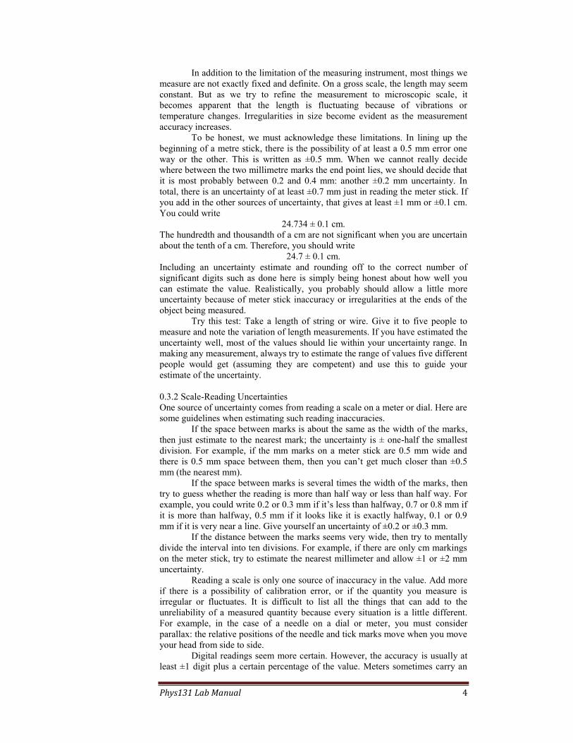
In addition to the limitation of the measuring instrument, most things we
measure are not exactly fixed and definite. On a gross scale, the length may seem
constant. But as we try to refine the measurement to microscopic scale, it
becomes apparent that the length is fluctuating because of vibrations or
temperature changes. Irregularities in size become evident as the measurement
accuracy increases.
To be honest, we must acknowledge these limitations. In lining up the
beginning of a metre stick, there is the possibility of at least a 0.5 mm error one
way or the other. This is written as ±0.5 mm. When we cannot really decide
where between the two millimetre marks the end point lies, we should decide that
it is most probably between 0.2 and 0.4 mm: another ±0.2 mm uncertainty. In
total, there is an uncertainty of at least ±0.7 mm just in reading the meter stick. If
you add in the other sources of uncertainty, that gives at least ±1 mm or ±0.1 cm.
You could write
24.734 ± 0.1 cm.
The hundredth and thousandth of a cm are not significant when you are uncertain
about the tenth of a cm. Therefore, you should write
24.7 ± 0.1 cm.
Including an uncertainty estimate and rounding off to the correct number of
significant digits such as done here is simply being honest about how well you
can estimate the value. Realistically, you probably should allow a little more
uncertainty because of meter stick inaccuracy or irregularities at the ends of the
object being measured.
Try this test: Take a length of string or wire. Give it to five people to
measure and note the variation of length measurements. If you have estimated the
uncertainty well, most of the values should lie within your uncertainty range. In
making any measurement, always try to estimate the range of values five different
people would get (assuming they are competent) and use this to guide your
estimate of the uncertainty.
0.3.2 Scale-Reading Uncertainties
One source of uncertainty comes from reading a scale on a meter or dial. Here are
some guidelines when estimating such reading inaccuracies.
If the space between marks is about the same as the width of the marks,
then just estimate to the nearest mark; the uncertainty is ± one-half the smallest
division. For example, if the mm marks on a meter stick are 0.5 mm wide and
there is 0.5 mm space between them, then you can’t get much closer than ±0.5
mm (the nearest mm).
If the space between marks is several times the width of the marks, then
try to guess whether the reading is more than half way or less than half way. For
example, you could write 0.2 or 0.3 mm if it’s less than halfway, 0.7 or 0.8 mm if
it is more than halfway, 0.5 mm if it looks like it is exactly halfway, 0.1 or 0.9
mm if it is very near a line. Give yourself an uncertainty of ±0.2 or ±0.3 mm.
If the distance between the marks seems very wide, then try to mentally
divide the interval into ten divisions. For example, if there are only cm markings
on the meter stick, try to estimate the nearest millimeter and allow ±1 or ±2 mm
uncertainty.
Reading a scale is only one source of inaccuracy in the value. Add more
if there is a possibility of calibration error, or if the quantity you measure is
irregular or fluctuates. It is difficult to list all the things that can add to the
unreliability of a measured quantity because every situation is a little different.
For example, in the case of a needle on a dial or meter, you must consider
parallax: the relative positions of the needle and tick marks move when you move
your head from side to side.
Digital readings seem more certain. However, the accuracy is usually at
least ±1 digit plus a certain percentage of the value. Meters sometimes carry an

Phys131 Lab Manual 5
accuracy note on them. (Look at the bottom of the digital volt meters.) If the
accuracy is indicated as ±(2% + 1 digit) this means that you have to add ±2% of
the reading to ±1 in the position of the last digit of the reading to get the total
error. For example, a three-digit meter reads 25.3 mV then the accuracy is
±(0.02 x 25.3 + 0.1) = ±( 0.5 + 0.1) mV = 0.6 mV.
Your estimate of the uncertainty of a value may well be different from
someone else’s estimate. Generally, there is no exact value. Therefore, you need
to keep only one significant figure for the uncertainty estimate unless its first
digit is 1. In that case, keep two digits. If your estimate is a factor of two different
from the instructor’s, there should be no problem. However, if your estimate
differs from an instructor’s by a factor of ten, it will probably be questioned.
0.3.3 Significant Figures and Precision
When you write values, make sure that the number of significant figures
corresponds roughly with the error estimate. Even without an explicit error
estimate, the number of significant figures implies an uncertainty. For example
writing 24.73 cm implies 24.73 ± 0.05 cm. For intermediate values that will be
used in calculation, it’s a good idea to keep an extra significant figure to maintain
accuracy: 24.734 ± 0.05 cm. But final results should not keep unnecessary
figures.
Sometimes for large numbers, you may need to write zeros that are not
significant; e.g., 24000 ± 400 gm. In this case, it is better to write (24.0 ± 0.4) x
103 gm to avoid insignificant zeros.
0.4 Graphical Analysis
How do we interpret experimental results given that they have uncertainties?
Have you disproved conservation of linear momentum if you find that the initial
momentum is 0.105 kg-m/s and final momentum is 0.114 kg-m/s? Suppose you
determine the value of g in Lab 1 to be 9.93 m/s2 while the accepted value is 9.8
m/s2. Is the deviation significant? The important points are
1. you must consider the experimental uncertainties in order to
decide these questions and
2. you can only give an argument based on probability.
This section shows some standard graphical techniques that will help you
interpret experimental results. In the first part (0.4.1), we consider the case where
your result is a single quantity, for instance the density of aluminum, which will
be compared with its accepted value. In the next part (0.4.2), we assume that you
study the relationship between two quantities by varying one of them
systematically, for instance measuring the vertical velocity vy of a falling object
at various times t.
0.4.1 Graphical analysis of a single quantity.
Suppose Qm is the value you measured for some quantity or calculated from
several measured quantities. Let ±Q be the best estimate of the uncertainty of
Qm, and let Q be the accepted or assumed value. Draw a (horizontal) number
line marked in appropriate, easy-to-read units, choosing a scale such that Q
measures from 1 cm to 5 cm. Locate the three points Qm, Qm –Q, and Qm+Q
and plot them just above the number line, as shown.
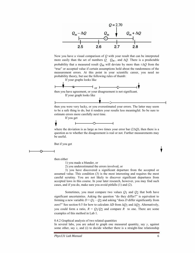
Phys131 Lab Manual 6
Now you have a visual comparison of Q with your result that can be interpreted
more easily than the set of numbers Q, Qm , and Q. There is a predictable
probability that a measured result Qm will deviate by more than ±Q from the
“true” or accepted value if certain assumptions hold about the randomness of the
measurement errors. At this point in your scientific career, you need no
probability theory, but use the following rules of thumb:
If your graphs looks like
or
then you have agreement, or your disagreement is not significant.
If your graph looks like
then you were very lucky, or you overestimated your errors. The latter may seem
to be a safe thing to do, but it renders your results less meaningful. So be sure to
estimate errors more carefully next time.
If you get
where the deviation is as large as two times your error bar (2Q), then there is a
question as to whether the disagreement is real or not. Further measurements may
be useful.
But if you get
then either
1) you made a blunder, or
2) you underestimated the errors involved, or
3) you have discovered a significant departure from the accepted or
assumed value. This condition (3) is the most interesting and requires the most
careful scrutiny. You are not likely to discover significant departures from
accepted laws in this course. In your later research, however, you may find such
cases, and if you do, make sure you avoid pitfalls (1) and (2).
Sometimes, you must compare two values Q1 and Q2 that both have
significant uncertainties. Asking the question “do they differ?” is equivalent to
forming a new variable D = Q1 – Q2 and asking “does D differ significantly from
zero?” See section 0.5 for how to calculate D from Q1 and Q2. Alternatively,
you could form a ratio, R = Q1/Q2 and compare R to one. There are some
examples of this method in Lab 1.
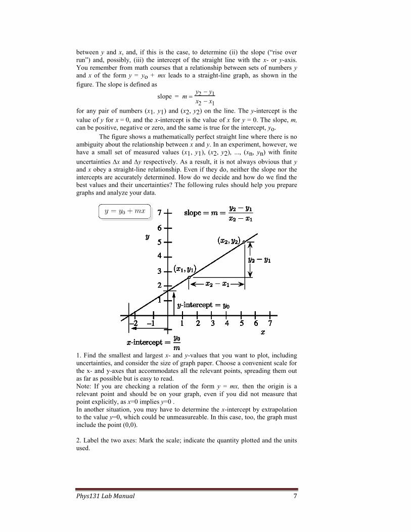
0.4.2 Graphical analysis of two related quantities
In several labs, you are asked to graph one measured quantity, say y, against
some other, say x, and (i) to decide whether there is a straight-line relationship
Phys131 Lab Manual 7
between y and x, and, if this is the case, to determine (ii) the slope (“rise over
run”) and, possibly, (iii) the intercept of the straight line with the x- or y-axis.
You remember from math courses that a relationship between sets of numbers y
and x of the form y = yo + mx leads to a straight-line graph, as shown in the
figure. The slope is defined as
slope = m y2 y1
x2 x1
for any pair of numbers (x1, y1) and (x2, y2) on the line. The y-intercept is the
value of y for x = 0, and the x-intercept is the value of x for y = 0. The slope, m,
can be positive, negative or zero, and the same is true for the intercept, yo.
The figure shows a mathematically perfect straight line where there is no
ambiguity about the relationship between x and y. In an experiment, however, we
have a small set of measured values (x1, y1), (x2, y2), ..., (xn, yn) with finite
uncertainties x and y respectively. As a result, it is not always obvious that y
and x obey a straight-line relationship. Even if they do, neither the slope nor the
intercepts are accurately determined. How do we decide and how do we find the
best values and their uncertainties? The following rules should help you prepare
graphs and analyze your data.
1. Find the smallest and largest x- and y-values that you want to plot, including
uncertainties, and consider the size of graph paper. Choose a convenient scale for
the x- and y-axes that accommodates all the relevant points, spreading them out
as far as possible but is easy to read.
Note: If you are checking a relation of the form y = mx, then the origin is a
relevant point and should be on your graph, even if you did not measure that
point explicitly, as x=0 implies y=0 .
In another situation, you may have to determine the x-intercept by extrapolation
to the value y=0, which could be unmeasureable. In this case, too, the graph must
include the point (0,0).
2. Label the two axes: Mark the scale; indicate the quantity plotted and the units
used.

Phys131 Lab Manual 8
3. Plot your data points (x1, y1), (x2, y2), ..., (xn, yn) with their uncertainties ±xi
, ±yi shown as error bars as in part 0.4.1. If x or y is too small to be plotted,
say so on the graph.
4. Now you are ready to check whether a straight line fits your data. Use a
transparent ruler to find the “best line” that passes closest to all your data points.
Remember that your “best line” must pass through the origin if you test a
relationship of the form y = mx. You can claim that a straight line fits your data if
it intersects at least 2/3 of your error bars. If a data point is far off the line, check
for errors in plotting it or recalculate it. If you find an error, correct and replot; if
not, ignore it and check whether a straight line fits the rest of the points. (But
comment on the presence of an outlier and on any possible explanations in your
notebook.)
5. Having found the best straight line for your data, determine the slope from
well-separated points on the line. (Use points on the straight line that you draw.
Do not use raw data points unless they are exactly on the line.) To find the
uncertainty in the slope, m, draw the steepest and shallowest lines that still pass
through more than half of the error bars. Let these lines pass through the origin if
you check a relation of the form y=mx and you are sure there is no zero-point
offset. Pick two well-separated points on the steepest line and two well-separated
points on the shallowest line in order to calculate the maximum and minimum
slopes mmax and mmin. Define m as (mmax – mmin)/2. For a typical set and a
reasonable choice of steepest, best and shallowest line you expect that m ≈ (mmax
+ mmin)/2. If this is not the case, reconsider your choice of lines. The next figures
show two hypothetical examples.
Graph 1: In this case both the slope and the intercept are determined by the data. The best fit line should touch at least 70% of the error bars. The maximum and minimum slope lines should touch about 50% of the error bars.
Graph 2: If the theoretical model only includes a slope the line of best fit must pass through the origin. If the best-fit line can’t touch at least 70% of the error bars, then perhaps the model is wrong. Points that look bad can sometimes be ignored, but the reasons should be discussed in your report.

Phys131 Lab Manual 9
0.5 Propagation of Errors: examples
Sum of two measurements
width w = 0.24 ± 0.03 m
length l = 0.89 ± 0.04 m
sum s = w + l = 0.24 + 0.89 m = 1.13 m
possible error of the sum is
s = w2 + l2 = 0.032 +0.04
2 = 0.05 m
The perimeter is twice the sum.
p = 2(w + l ) = 2s = 2.26 m
possible error of perimeter is
p = 2s = 0.1 m
In conclusion, write the perimeter as
p = 2.3 ± 0.1 m
Product of two measurements
width w = 0.24 ± 0.03 m so %..
.
w
w512
240
030
length l = 0.89 ± 0.04 m so %..
.
l
l54
890
040
Area is the product of width and length
A = wl =(0.24 m) (0.89 m) = 0.2136 m2
Possible error of area is given by
A
A =
w
w
2
+
l
l
2
A
A = 12.5%
2 + 4.5%
2 = 13 %
A = (0.13)(0.2136 m2) = 0.028 m2
So one should write
A = 0.21 ± 0.03 m2

Phys131 Lab Manual 10
What do you do with weird functions?
For example, what is the possible error of
x =cos()
when = 21° ± 2° ?
x = cos(21°) = 0.9335
The easiest way to find x is to substitute for the minimum and maximum values:
cos() = 1
2 | cos(23°) – cos(19°) |
= 1
2 | 0.9205 – 0.9455| =
0.025
2
= 0.0125
so write
x = 0.934 ± 0.012
Using Calculus to find cos():
x = cos() =
dcos()
d
Caution:
If you use calculus, must be in radians.
±2° = ±2π
180 = 0.035 radians
21° = 0.367 radians
x = cos() = | sin(0.367) (0.035)|
= |(0.359)(0.035)|
= 0.0125
write 0.012 or 0.013 as you wish.
0.6 Propagation of Uncertainties: General Rules
The uncertainty of calculated quantities depends directly on the uncertainties of
the variables used in the calculation. For brevity, we simply state the rules for
commonly encountered situations here. Later, some of these rules will be
justified, but a complete understanding needs statistical methods that are too
advanced for this course.
In the following, let A, B, C, ... stand for independent quantities with
uncertainties A, B, C, .... Let Y = f(A,B,C, ...) be the calculated quantity of
interest.

Phys131 Lab Manual 11
0.6.1 Rule 1: A constant multiple
If
Y= k A
where k is a constant, then
Y = k A
0.6.2 Rule 2: Addition and Subtraction
If
Y = A ± B ± C
then
Y = (A)2 + (B)2+ (C)2 .
The generalization to the sum of four or more quantities should be obvious. The
reason for taking the root-squared sum instead of just adding the uncertainties is that
we are not certain whether the errors will cancel or add. If there are many terms in
the sum, there will typically be some cancellation and the combined error will not
likely be as large as the error given by the sum |A |+ |B| + |C| + ... .
0.6.3 Rule 3: Multiplication and Division
If
Y = ABC, Y = ABC–1, Y = AB–1 C–1, or Y = A–1 B–1 C–1
then
Y
Y
A
A
2
B
B
2
C
C
2
For multiplication and division, we add the fractional (or percentage) errors.
0.6.4 Rule 4: Powers
If
Y = A, where is arbitrary: integer, fraction, positive or negative
then
Y
Y = ||
A
A
0.6.5 Examples
(1) Y = AB2
Let C = B2 so that Y = AC.
Then according to rule 3 Y
Y
A
A
2
C
C
2
.
According to rule 4 C
C = 2
B
B
Therefore Y
Y
A
A
2
4B
B
2
.
Example (2) Y = 1
A +
1
B
Let C = A–1 and D = B–1.
According to rule 4 A
A =
C
C and
B
B =
D
D .
However, C = A–1 and D = B–1 so that these latter two expressions can be
written as

Phys131 Lab Manual 12
C = A/A2 and D = B/B2.
Hence,
Y A
A2
2
B
B2
2
.
0.6.6 The General Case
The four rules and the rule for the general case can be derived with the help of
calculus. In this discussion, we will assume a function of the form
Y = f(A,B) (1)
Generalization to functions of more variables is easy.
Calculus tells us that if we change A by a small amount dA and B by dB
then the change in Y is given by
dY =¶f
¶A
æ
èç
ö
ø÷B
dA+¶f
¶B
æ
èç
ö
ø÷A
dB,
(2)
where the subscript A or B on the partial derivatives has the conventional
meaning that the quantity A or B is to be held fixed while taking the derivative.
(That is the definition of partial derivative.) For convenience these subscripts are
omitted from now on.
This equation tells us how fast the function Y changes when we change
its inputs A and B by some small amounts dA and dB. We can identify these small
changes with small errors in our measurements, ±A and ±B. These errors can
have either algebraic sign and so can the derivatives (∂f/∂A) and (∂f/∂B). In the
worst case both terms in (2) are positive or both negative in which case you have
Yworstcase f
A
A
f
B
B . (3)
On the other hand it could turn out that you are lucky and the two terms in
equation (2) tend to cancel. Then you would have
Ybestcasef
A
A
f
B
B
.
(4)
In practice, there is no way of knowing whether the errors are going to
cancel or add in the final answer. Probability theory says that in such a case, if the
errors are independent and have a normal distribution, then we should add the
individual errors “in quadrature”; i.e., form the root-squared sum as
Y f
A
A
2
f
B
B
2
.
(5)
Note that Y has the property
Yworst case ≥ Y ≥ Ybest case.
You can visualize this way of adding errors by means of a right triangle.
Y
f
A
A
f
B
B
Phys131 Lab Manual 13
The generalization of equation (5) to an arbitrary number of variables Y =
f(A,B,C...) is
Y f
A
A
2
f
B
B
2
f
C
C
2
.. . (6)
With a little effort, you should be able to convince yourself that rules 1 through 4
are but special cases of Equation (5), which can also be used for more general
cases such as trigonometric or exponential functions.
0.7 Systematic and Random Uncertainties Broadly speaking, one encounters two types of uncertainties: systematic and
random. People usually talk about systematic and random errors. The term
"error" is unfortunate because there usually is no mistake involved. Rather, any
measurement has limitations and returns a value that must be understood as
covering a range of possible "true" values. Hopefully, this will become clearer as
we proceed. In any case, we will bow to custom and use "error" rather than
"uncertainty" in our discussion.
0.7.1 Systematic errors
"Systematic" errors are those that are repeatable from measurement to
measurement. For example, if you are using a metre stick, the scale could be off.
Where it reads 1 cm, for example, the true value might actually be 1.1 cm. If that
were the case, every time you measured an object, you would be 10% too low.
That 10% would be perfectly repeatable, since it comes from the entire scale's
being incorrect.
Although this sounds like an artificial example, that is only because we
have exaggerated the size of the effect. If you take a long tape measure (say 4
meters in length), then it may well read 12 meters when it is actually 12.001 m.
Another type of systematic error can arise in a calculation. For example,
let's say that you are measuring the period of a pendulum's oscillation. The
simplest theory of the pendulum predicts the period to be independent of the
amplitude of oscillation. That calculation turns out to be correct, but only for
infinitesimally small oscillation amplitudes. At finite amplitudes, there is in fact
a small dependence. Because you must measure the period using a finite
amplitude, there will always be a systematic difference between what you
measure and the prediction based on the simple theory. If one had a more
sophisticated theory that gave the dependence on amplitude, this systematic error
would vanish. Absent such a theory, one could investigate how much of an error
exists and try to conduct the measurements in a regime where other errors were
larger.
0.7.2 Random errors
"Random" errors are those that give a different result every time. You measure
something and record the result. You do exactly the same thing again and get a
slightly different result. Of course, if you did "exactly" the same thing, you
would expect to get the same result. But usually, it is impossible to do things
exactly the same twice. If there are many small, uncontrollable effects, they will
produce small differences in the results of repeated trials of the same
measurement.
One example of a random error, which we will encounter in the first lab,
arises when using a stopwatch to time events. Let us think (and try!) the
following experiment: Your instructor will drop a ball from a height (say 2
meters) onto the floor. Each student has a stopwatch and times, independently,
this same event. (Equivalently, one student could time the fall of many balls, but

Phys131 Lab Manual 14
this takes longer and is less fun!) When the instructor yells "go!" he or she drops
the ball, and you start your stopwatch. When the ball hits, you hear the sound
and you stop. Let's say that there are 30 people in the class. They may get the
following results (in seconds):
0.64, 0.62, 0.63, 0.67, 0.58, 0.48, 0.53, 0.63, 0.58, 0.57, 0.73, 0.74, 0.71, 0.59,
0.68, 0.63, 0.57, 0.56, 0.65, 0.76, 0.77, 0.62, 0.52, 0.68, 0.56, 0.58, 0.79, 0.58,
0.64, 0.76
The first thing to note is that the numbers differ, and by a fair amount.
They range from 0.48 s to 0.79 s, a difference of almost 70%! Does that mean
one cannot say anything about the "true" value? Not at all! Using some
elementary ideas from statistics, we can actually say quite a lot.
The first thing to do when confronted with such results -- called
"repeated trials" in the jargon of statistics -- is to group them in a histogram. To
do this, we set up bins and count how many measurements fall into each bin. For
example, we can choose a bin size of 0.05 s. In Fig. 1a, we show the resulting
histogram. Using this histogram, we can try to better characterize the collective
results of the 30 trials.
Fig. 1: Observations grouped in bins of 0.05 sec. (a) raw histogram; (b)
histogram overlaid by bell curve that describes the result of an experiment with
infinitely many trials. The wide horizontal line is the standard deviation of the
observations, while the narrow horizontal line is the standard deviation of the
average of the observations.
10
8
6
4
2
0
Me
asu
rem
ents
pe
r b
in
0.90.80.70.60.50.4
Time (s)
10
8
6
4
2
0
Me
asu
rem
ents
pe
r b
in
0.90.80.70.60.50.4
Time (s)
(a)
(b)

Phys131 Lab Manual 15
In (a), we see that the distribution is starting to form a "bell-shaped
curve," although 30 trials is still so small that it is not a "pretty" curve, but there
are large variations from the "ideal" shape (overlaid in part b).
The next thing to do is to try to extract a "typical" value. Statistics
teaches us that the "best" value we can use is the average. If ti is the i'th time
measurement (i from 1 to 30 in this case), then the average is
where N = 30, in this case. For the measurements above, the average is 0.635s.
The next thing that one can extract is a typical value for the trial-to-trial
"fluctuation." In other words, if one takes a typical trial, how far away is it from
the true value? This quantity is known as the "standard deviation." Graphically,
it is the width of the best bell-shaped curve. In statistics, one can show that the
best estimate from the data is the "standard deviation", ,
In words, one calculates the average and takes the difference between
each point and the average. One squares this difference and adds it to a sum over
all data points. This sum is normalized by N-1 (not N; it's a bit of a long story but
comes about because the average is estimated from the data, rather than being
known exactly). For the above data, one estimates = 0.08 s. This is the typical
deviation of each measured trial from the "exact" value. Any single
measurement, for example the second one (0.62s), would be reported as, say, 0.62
± 0.08s.
Finally, the average value should intuitively be closer to the real value than
any single measurement. The rules for error propagation (see 0.6.1 and 0.6.2) tell
us that the uncertainty in the average should be the uncertainty in a single
measurement divided by the square root of the number of measurements, i.e.,
For the events here, this is 0.08/ (30)0.5
= 0.015 s. Thus, an individual
measurement is likely to be off by about ± 0.08s, but the average (for 30 trials)
will typically be off by only 0.015s. The average, with the error bars for a single
measurement and for the average itself are both shown in Fig. 1b (filled marker
and hollow marker, respectively). For the average, we would report 0.635 ±
0.015s. (A more honest estimate of these numbers would be 0.64 ± 0.02 s, since
the original uncertainty (0.08s) was only to one significant figure).
We can also see, in Fig. 2, how increasing the number of measurements
produces histograms that converge slowly to the bell-shaped solid curve. Many
trials are required to get a nice-looking convergence.
1
N 1ti t
i1
N
2
avg
N
t 1
Nti
i1
N

Phys131 Lab Manual 16
Fig. 2: Effect of increasing the number of trials. (a) 30 trials; (b) 300 trials; (c)
3000 trials. Notice how the histograms converge to the bell curve, which shows
what would be observed after an infinite number of trials. The y-axis of the
histograms have all been normalized by dividing the bin height by the number of
trials for each case. Bin size is 0.01 sec. (compare with 0.05 sec. in Fig. 1).
Note: By doing more and more trials, the random error can be reduced to
very small values. In practice, it is not worth going below the point where other
errors (particularly systematic errors) start to dominate.
10
5
0
0.90.80.70.60.50.4
10
5
0
0.90.80.70.60.50.4
Time (s)
10
5
0
0.90.80.70.60.50.4
30
300
3000
(a)
(b)
(c)

Phys131 Lab Manual 17
Error Analysis Problems
1. The scale shown is from a pressure gauge. The reading is in microns (µm) of
mercury. State the value and uncertainty limits of the reading at positions a, b, c,
d and e.
2. Specifications on the bottom of a Fluke digital multimeter say:
ACCURACY: ±(% OF READING + DIGITS)
DC VOLTAGE: (0.1 + 1)
DC CURRENT: (0.3 + 1) EX (0.5 + 1 @ 10A)
Decipher this inscription and rewrite the following readings with the correct
number of significant figures and state the uncertainty. a) 2.125 V, b) 0.002
mV, c) 0.615 A, d) 21.21 V, e) 9.892. A
3. Determine the values and uncertainties of the following derived quantities from
the stated values and uncertainties of the respective measured quantities.
a) voltage, V = 5.6±0.1 V, current I = 0.125 ±0.02 A, power, P = ? ± ?
b) time, t = 3.67±0.05 s, distance x = 4.52±0.01 m, velocity, v = ? ± ?
c) distances: x = 6.24±0.05 m, y = 7.8±0.1 m, z = 4.03±0.01m area,
A = x2 + yz = ? ± ?
d) distances: x = 6.24±0.05 m, y = 7.8±0.1 m, z = 4.03±0.01m geometric
mean <x> = (xyz)1/3 = ? ± ?
e) amplitude, A = 9.000± 0.001 m, time, t = 26.0 ± 0.5 s distance,
d = A sin(t/16) = ? ± ? (angle in radians)
f) amplitude, A = 9.000± 0.001 m, time, t = 51.0 ± 0.5 s distance,
d = A sin(t/16) = ? ± ? (angle in radians)
4. a) Five measurements of diameter are made with an estimated reading
accuracy of ±0.3mm: 3.20, 3.19, 3.21, 3.22, 3.20 cm. What is the average and
its uncertainty?
b) Six measurements are made on another sample with the same reading
accuracy: 3.21, 3.68, 2.69, 3.43, 3.52, 3.54 cm. What is the average and its
uncertainty?
5. Gold is denser than lead and more expensive. You wish to determine whether
a wafer of gold has been diluted with lead by measuring its density. The wafer is
supposed to be 25 g of pure gold, and you can measure its volume with an
uncertainty of ±0.2 ml and its mass within ±0.1 g. What is the largest admixture
of lead that can escape detection expressed as a fraction of total mass?

Phys131 Lab Manual 18

Phys131 Lab Manual 19
Lab 1 – Pendulums References
E. M. Rogers, Physics for the Inquiring Mind. (Princeton University
Press, Princeton, NJ, 1966). Permission of citation granted by estate of
Eric M. Rogers.
P. A. Tipler, Physics for Scientists and Engineers, 6th Ed. Ch 14,
Oscillations.
Resnick, Halliday and Krane, Physics, 5th Ed. Ch 17, Oscillations.
Objective
An "Open Lab" where you will be able to plan and do your own
experiment, make your own mistakes, criticize the mistakes of others,
and maybe learn from them.
Apparatus
String, weights, ring stand, meter stick, stopwatch, electronic timer,
anything else we have.
Method
You fill in this section.

Phys131 Lab Manual 20
EXPERIMENT: PENDULUMS
Narrow your field of investigation down to a simple pendulum, a small bob
swinging to and fro on a long thread; and narrow it still more to the question,
"How does the time-of-swing or period of a pendulum depend on each of the
physical factors that might affect it?" Thus restricted, this is still a complex
investigation unless you follow the good scientific practice of holding all other
factors constant while you change one chosen factor at a time. See Fig. 4-2.
We define the PERIOD as the time of one "swing-swang," one complete
cycle. What factors might affect the period? Obviously, the LENGTH of the
pendulum -- most easily defined as distance from support to center of bob, but
not easily, or wisely, measured directly in that form. We all know a longer
pendulum takes more time to swing to-and-fro. But just how is the period T
related to the length L? Is there a simple mathematical rule? (There is. We can
deduce it from other experimental knowledge, e.g., from force vectors and
Newton's Laws of Motion; but here you should make an "empirical investigation"
-- ask a straight question of nature in your own experiments.)
What other factors might affect T? Mass or weight of bob; amplitude, or
size of swing; and possibly other factors?
Start by investigating how T depends on
length of pendulum, L
amplitude of swing, A° each side of vertical
mass of bob, M
To avoid confusing several effects, keep two of the three, L, A, M,
constant while you change the third, and measure T. Does it matter which of the
three you choose to vary first? In this case, it does: there is one logically correct
choice. While you are considering this, make some preliminary measurements to
try out techniques.
(0). Preliminary Measurements
A good scientist does not expect a stream of accurate measurements to flow at
once from his apparatus. He experiments on his experiment, trying out
techniques, gaining skill by practice. Choose a long pendulum, 2 or 3 ft long, and
make accurate timings of its period with a good stopwatch (or use a magnifying
glass over the seconds hand of an ordinary watch while a partner gives you
signals.) Record your measurements. Compare them with your partner's. Look at
the methods being used by neighbours, and get ready to criticize.
Discussion Group
When you have practical experience of your apparatus, meet with other students
and the instructor, as a "research team" to discuss difficulties and techniques.
This is the time to suggest good tricks you have discovered, to criticize mistakes
you saw neighbours making, to discuss the reliability of the equipment, and to
decide on good techniques and plan the order of experiments. There is little use
in such a discussion before you have done preliminary experimenting: that would
lead to childish guessing, or else your instructor would have to step in with
cookbook directions. As in a professional research group, an adult discussion
needs practical experience of the apparatus.
At this time, you will find there is a good reason for investigating the
effect of AMPLITUDE first, before MASS or LENGTH.
(1). Measurements: T vs. A
Make careful measurements of T for the following amplitudes: 70°, 60°, 50°, 40°,
30°, 20°, 15°, 10°, and 5°. Plot a rough graph of T vs. A as you go, to guide your

Phys131 Lab Manual 21
further measurements. If you find the graph-points use only a narrow region of
your paper, you should plot another graph with one coordinate expanded so that
the blown-up graph reveals the shape better. (A blown-up graph need not have
the origin on the paper--in fact its origin may be many inches off the paper.) If
you run into difficulties, discuss them with your instructor--treat him or her as a
source of good advice from another scientist, not as a short cut to "right answers".
When you have enough good measurements, plot a careful graph of T
against A — with a blown-up version, too, if that seems called for.
At this stage, another conference is likely to be useful. Comparing your
graph with the graphs of others, you will probably decide there is a definite
relationship, but many graphs may show such large accidental errors that their
form is obscured. An accurate answer to "How does T depend on A?" is
essential: the other parts of this investigation will be impossible without it. You
will need very careful measurements of T for a certain range of amplitudes. It
will be obvious from your present graphs what that range is, and why
measurements outside that range need not be very accurate.
More accurate measurements
With increased skill from practice and better knowledge of techniques, make the
measurements needed to settle the essential question about T and A, and plot them
in the graph of T against A. (This sounds like a long piece of drudgery, fussing
over better precision. It will take time and trouble, but the outcome is
rewarding.) When you have settled the question, write your answer or conclusion
clearly, and use it in part (2).
(2). Measurements: T vs. M
How much faster would you expect a heavy bob to pull the pendulum to and fro
than a light one? Measure T for a fairly long pendulum, using the conclusion of
your T vs. A experiments to guide your arrangements. (Of course, you should not
repeat your T vs. A investigation all over again for each bob in this investigation.
Once that is settled it is settled, and its results can be used without repeating the
investigation.)1 Change to another bob much heavier or much lighter, and repeat
your measurements. Make sure that the L, from support to centre of bob, is the
same for both. (That is why we offered the cookbook suggestion of a long
pendulum: the longer the thread the smaller the % change in L if you make a
small mistake in changing bobs.)
(3). Measurements of T vs. L
The period T changes greatly as L changes and a good graph (or other
investigation) of the relationship between them needs many sets of
measurements. Here is where cooperation among the whole laboratory group is
welcome. With the answers to questions or parts (1) and (2) known, it is easy to
pool comparable measurements from every member of the group.
Each student (or pair) should measure T for one length, and then the
group should pool their measurements for graphs. One student should choose a
length between 1 metre and 0.9 m; another student between 0.9 and 0.8 metre;
and so on. Then everyone in the group will need a record of all results, to plot a
graph of T against L and to look for the relationship.
"The Pendulum Formula" and Measuring g
Phys131 Lab Manual 22
There is a definite relationship between T and L, a well-known one that you are
likely to meet in physics books or as an example in algebra books. If you do not
already know it, try guessing at it from the numbers in the communal record, or
from the shape of your graph. Then plot a second graph of something else (1/T?,
T ?, ... ?) against L that you expect to give a straight line. Or, if you prefer, ask
an instructor to tell you the relationship -- as a piece of well-known hearsay --
and use it to plot a straight-line graph. Draw the "best straight line" that runs "as
near as possible to as many points as possible."
The pendulum formula relating T and L also contains "g," and pendulum
timings offer very precise methods of measuring g even today. If you do not
know it, get the full formula from your instructor and calculate "g" from your
straight-line graph. For that you need first the slope of that line--by using the
slope instead of single measurement, you are taking a weighted average of many
measurements. Also calculate "g" from your own single measurement that you
contributed to the pool.
1We assume that the factors A and M, L, etc. affect T independently, so that
changing M here does not affect the T vs. A story. That is often a safe assumption
in physics. In some other fields of study — such as biology, psychology, or
economics — this would be a very dangerous assumption.

Phys131 Lab Manual 23
Lab 2 – DC Circuits
References Tipler (6th Ed), Chapter 25: Electric Current and Direct-current Circuits
Halliday, Resnick and Krane, (5th Ed.) Chapter 31, DC Circuits
Objective
Fundamental principles of direct current electrical circuits are explored
using digital and analog meters.
THEORY
An electric current I is a flow of charge Q through a section of conductive
material. If charge is measured in coulombs (C) and time in seconds (s), then one
coulomb of charge flowing through the entire cross section of a wire per second
is defined to be a current of one ampère (A) flowing through that wire.
1 A = 1 C/s.
The potential difference V between any two points in a circuit is the work
required to move charge from one point to the other. If the potential difference is
negative, energy is released during the movement of the charge, and current will
move spontaneously. Potential difference is measured in volts. A potential
difference of one volt (V) between two points means that it takes one joule (J) of
work to move one coulomb of charge between the two points.
1 V = 1 J/C
A useful analogy to electric current flow is the flow of liquid. Current
through a wire is like flow through a pipe and a voltage difference between two
points of a wire is like a pressure difference between two points of a pipe. Most
of the laws of dc circuits can be visualized by reference to the fluid flow analogy. Kirchhoff’s Laws
The two most fundamental laws of circuits are Kirchhoff’s laws. These results
from the conservation of energy and charge, as applied to electrical circuits. You
may find it useful to think about the analogy to fluid flow.
1. Conservation of energy
The sum of voltages around any closed loop is zero.
2. Conservation of charge
The total current flowing into a junction equals the current flowing out of
it.
Ohm’s Law
The current flowing through an electrical wire or devices is often directly
proportional to the voltage across it. Such electrical devices are said to obey
Ohm’s law: Their electrical resistance R is defined as V/I. Ohm’s law says that
this resistance is constant. Resistance is measured in ohms (Ω).
1 Ω = 1 V/A.
Many electrically conducting materials and devices do not obey Ohm’s law—the
ratio of voltage to current is not constant. Resistors are electrical components that
are manufactured to have constant resistance over a wide range of operating
conditions.
Series and Parallel Resistances
Series: When two resistors are connected in series, so that all current that
passes through one must also pass through the other, the resistance of the
combination is the sum of each resistance: R = R1+ R2.

Phys131 Lab Manual 24
=
Parallel: When two resistors are connected in parallel so that current can
flow through either one or the other, the inverse resistances add: 1/R = 1/R1 +
1/R2.
Meters
Three types of meters are used for electrical measurements. Voltage is measured
with a voltmeter; current is measured with an ammeter; and resistance is
measured with an ohmmeter. Modern meters are digital multimeters, which
means that they can function as a voltmeter, an ammeter or an ohmmeter
depending on which function is chosen on the front panel switches.
Voltmeters
A voltage is measured by connecting a voltmeter to two points on the circuit.
Nothing needs to be disconnected for the voltage measurement; just make
electrical contact between the test leads to the points desired.
Figure 1(a) shows a voltage source (a battery) connected to two resistors.
In order to measure the voltage across R2, connect a voltmeter as shown in Figure
1(b). The black dots are electrical connections. Figure 1(c) illustrates the meaning
of the schematic in 1(b). Ideally, one wants the voltage across R2 in circuit (a) to
be the same as in (b). In reality, the voltmeter changes the voltage slightly
because it conducts some current through it, diverting the current away from R2.
R R1 2 R = R1 R2+
R1
R2
R =R1 R2
R1 R2+
=
Fig. 1: Using a voltmeter to read voltage

Phys131 Lab Manual 25
Fig. 2: The internal resistance of a voltmeter
Saying that the voltmeter conducts some current is the same as saying that there
is an internal resistance in the meter Rm that is less than infinite. An ideal
voltmeter would not conduct current, so its internal resistance would be infinite.
The figure above symbolizes this internal resistance with a grey resistor symbol.
When the voltmeter is connected to both ends of R2, the equivalent resistance
between these two points becomes R2Rm
R2 + Rm which is less than R2. Therefore,
the voltage read by the real meter is less than what would be read by an ideal
meter. In order to be useful, the voltmeter’s internal resistance must be much
larger than the resistance between the points in the circuit where it is connected:
Rm >> R2. The bigger the meter’s resistance, the better. The digital voltmeters in
the lab have resistances of 10 MΩ. The little analog voltmeters have resistances
of about 50 kΩ.
Ammeters
Fig. 3: How to use an ammeter
An ammeter measures the current flowing through it. Figure 3 shows that the
ammeter is used to replace the wire between the two resistors. Therefore, current
is forced to flow through the ammeter. Ideally the ammeter should be a perfect
conductor — zero resistance — but, in fact, real ammeters have some internal
resistance. In order for the current measured by the ammeter to be close to the
+
VV
R1
R2 Rm

Phys131 Lab Manual 26
current in the circuit without the ammeter, its internal resistance should be small:
Rm << R1 + R2. The digital meters have a resistance of about 1 Ω on the amp
scale and 1.2 kΩ on the mA scale.
Ammeters usually require more effort to use than voltmeters because you
must take out a connection in the circuit and replace it with the meter. Voltmeters
simply require touching two points in the circuit. Therefore, most people try to
minimize the number of current measurements they need to make.
Ohmmeters
Resistances are measured by an ohmmeter. Most multimeters have an ohmmeter
setting. The resistance is measured by passing a small current through the resistor
and measuring the voltage across it.
In order to measure the resistance of a component in a circuit, you must make
sure that at least one of its leads is disconnected from the circuit. Otherwise, you
will measure the resistance of that component in parallel with the rest of the
circuit.
Experiment
The Potentiometer
The fine nichrome wire provided has a resistance of several ohms per
Fig. 4: How to use an ohmmeter
+
V+
žV
(a) (b)Ohmmeter
Open CircuitR1
R2
R1
R2

Phys131 Lab Manual 27
meter. Attach a length of nichrome wire between the banana-plug terminals
spanning the length of the board over the tape measure scale. Try to get the wire
as straight and tight as possible. You have now made a potentiometer. Connect
the DC power supply to the ends of the potentiometer. Now connect the negative
terminal of the digital multimeter to the negative end of the potentiometer. The
positive terminal of the voltmeter should go to a banana plug wire with an
alligator clip on the other end that can be pressed against the potentiometer wire
at any point along its length. The alligator clips fit on banana plugs at each end of
the connecting wires. Since the banana plugs have holes into which other banana
plugs can fit, you don’t need to clip alligator clips onto other alligator clips.
Put the multimeter in the D.C. voltage mode, and adjust the power
supply to deliver 5 V across the length of the potentiometer using the following
steps:
1. Turn the voltage knob down to zero
2. Turn the current limit knob to zero.
3. Turn on the power supply
4. Turn up the current limit knob a little.
5. Adjust the voltage setting knob until you read about 5 V on the power
supply’s voltmeter.
If you can’t get to 5 V, try increasing the current limit a little. If the current keeps
increasing no matter how high the current is set, something is wrong. Make sure
the current isn’t being limited by the power supply—if the circuit is correct and
the current limit is set high enough the current shouldn’t depend on its setting.
6. Connect the digital meter across the whole potentiometer and adjust the
voltage until it reads exactly 5 V.
Touch the positive terminal of the voltmeter to five equally-spaced
positions along the potentiometer. Record the position in meters or centimeters
and the voltage read on the digital meter. Plot a graph of the voltage vs. position
along the potentiometer.
Disconnect the multimeter and reconnect it to measure the current
through the potentiometer. Use the A scale not the mA scale, or you’ll blow the
fuse! Don’t change the setting on the power supply. After measuring the current
for 5 V, you can calculate the resistance of the nichrome wire using Ohm’s law.
Connect the multimeter to the potentiometer so as to measure the
resistance directly using the ohmmeter function.
Compare the resistance measured directly with that calculated from the
current and voltage. Explain why there may be a difference between the two
values.
I vs V for a Resistor and a Light Bulb
Connect the variable power supply across a 10 kΩ resistor. (Support the resistor
on the screw terminals on the experimental board.) Use the analog Armaco
milliammeter to measure current through the resistor and the digital multimeter to
measure the voltage across the resistor. Draw a schematic diagram of the circuit
in your notebook. Measure the current through the resistor for five different
voltage settings. Plot a graph of I vs. V and use it to find the resistance.
Find the current-voltage characteristics of a light bulb. You will have to use
another way to measure the current because it will be much larger! Connect a
circuit so that you can measure the light bulb current for voltages between 0 and
40 V in steps of 5 V. Plot I vs. V. Can you explain why this isn’t a straight line?
What is the lamp’s resistance? Does that question make any sense? Now replot
the data in the form of log I vs. log V. Does this form a straight line? If so, write
the equation describing the functional relation.

Phys131 Lab Manual 28
Series and Parallel Resistances
You have two 10 kΩ resistors and one 1 kΩ resistor. Calculate the resistance you
expect in each of the following cases and then measure it with the ohmmeter.
1. 10 kΩ in series with 10 kΩ,
2. 10 kΩ in series with 1 kΩ,
3. 10 kΩ in parallel with 10 kΩ,
4. 10 kΩ in parallel with 1 kΩ.
Answer the following questions:
1. If two nearly equal resistors are in series, what is the approximate equivalent
resistance?
2. If a resistor is in series with a much smaller resistor, what is the approximate
equivalent resistance?
3. If two nearly equal resistors are in parallel, what is the approximate equivalent
resistance?
4. If a resistor is in parallel with a much bigger resistor, what is the approximate
equivalent resistance?
The Wheatstone Bridge
The Wheatstone bridge is useful for measuring very small changes in resistance.
The figure shows the physical connections and the schematic for a Wheatstone
bridge. You should be able to prove that the voltmeter will read 0 V when the
ratio of the resistances on the left- and right-hand sides of the potentiometer is the
same as the ratio of R1 and R2. If the resistance wire has a uniform resistance per
unit length and the lengths on the left and right are l1 and l2 then:
V = 0 when R1
R2 =
l1
l2
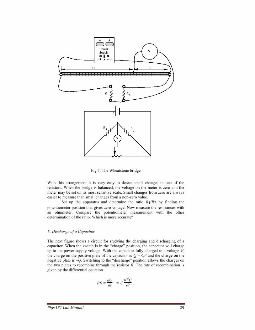
Phys131 Lab Manual 29
Fig 7. The Wheatstone bridge
With this arrangement it is very easy to detect small changes in one of the
resistors. When the bridge is balanced, the voltage on the meter is zero and the
meter may be set on its most sensitive scale. Small changes from zero are always
easier to measure than small changes from a non-zero value.
Set up the apparatus and determine the ratio R1/R2 by finding the
potentiometer position that gives zero voltage. Now measure the resistances with
an ohmmeter. Compare the potentiometer measurement with the other
determination of the ratio. Which is more accurate?
V. Discharge of a Capacitor
The next figure shows a circuit for studying the charging and discharging of a
capacitor. When the switch is in the “charge” position, the capacitor will charge
up to the power supply voltage. With the capacitor fully charged to a voltage V,
the charge on the positive plate of the capacitor is Q = CV and the charge on the
negative plate is –Q. Switching to the “discharge” position allows the charges on
the two plates to recombine through the resistor R. The rate of recombination is
given by the differential equation
I(t) = dQ
dt = C
dVC
dt .

Phys131 Lab Manual 30
It can be shown that the voltage on the capacitor will decay according to the
formula
VC(t) = V0 e–t/RC
where V0 is the power supply voltage and t = 0 is the time that the switch moves
from charge to discharge. The numerical constant e is about 2.71. The voltage
will decay from V0 to V0/e in the time RC, where RC is the “time constant” of the
circuit.
Connect the circuit using a 100 kΩ resistor and the capacitor supplied to
you. The capacitor may be “electrolytic,” which means that it should be
connected with the polarity indicated on its case. Sometimes a black stripe
indicates the negative end.
To determine the time constant, first charge the capacitor to 27.1 V with
the switch in the “charge” position. Switch to “discharge” and time how long it
takes for the voltage to fall to 10 V. (10 V = 27.1/e V.) Do this about three times
to check the reproducibility. If the time is too fast to measure, then there is either
a mistake in the wiring or you need a larger capacitor. Compare your measured
time constant with what you calculate from the indicated resistor and capacitor
values. (The accuracy of the indicated capacitor value is only about ±20%.)
Now connect the Armaco analog voltmeter to measure the voltage
instead of the digital multimeter. Measure the time constant a few times and
compare this with the previous measurement. If there is a difference in the two
values, decide which is correct and why.

Phys131 Lab Manual 31
Prelab Questions
1. The potentiometer extends between positions 1.9 cm and 54.6 cm on the
scale. In part I (The Potentiometer) the voltage read by the DMM is 5.000 V and
the current read the by DMM is 0.425 A. What is the resistance per unit length of
the nichrome wire? (Does the DMM affect the resistance measurement?)
b) The accuracy of the multimeter is cited as ±0.1% ±1 digit on the
Voltage scale and ±0.3% ± 1 digit for the Amp scale. What are the uncertainties
of the voltage and current readings and the resultant uncertainty of the resistance
of the wire?
2. Calculate the four equivalent resistances required for the “Series and Parallel
Resistances” section.
3. In the Wheatstone bridge experiment R1 = 10 kΩ , l1 = 14.2 cm and l2 =
83.5 cm. What is the value of R2?
Resistor Colour Code Useful Values:
brown-black 1 0
red-red 2 2
yellow-violet 4 7
With these three combinations of the first two bands, together with different
multipliers, you can cover the whole range with steps of a factor two. For
example,
1 kΩ = 10x102 brown-black-red
2.2 kΩ = 22x102 red-red-red
4.7 MΩ = 47x105 yellow-violet-green
It's useful to keep in mind at least two common ranges for the third band
multiplier:
red kΩ range (1-9.9 kΩ)
green MΩ range (1-9.9 MΩ)
Except for high precision resistors, only certain values of resistors are
commonly available. Standard Resistance Values for the first two digits are
10%, 2% and 5%: 10, 12, 15, 18, 22, 27, 33, 39, 47, 56, 68, 82 2% and 5% only: 11, 13, 16, 20, 24, 30, 36, 43, 51, 62, 75, 91

Phys131 Lab Manual 32
digit colour multiplier # zeros silver 0.01 –2 gold 0.1 –1 0 black 1 0 1 brown 10 1 2 red 100 2 3 orange 1k 3 4 yellow 10k 4 5 green 100k 5 6 blue 1M 6 7 violet 10M 7 8 grey 9 white
Resistor Colour Code
1st & 2nd digit
multipliertolerance: red = 2% gold = 5% silver = 10% none = 20%
orange or yellow band indicates MIL spec reliability rating

Phys131 Lab Manual 33
EQUIPMENT NOTE: 33XR Meterman Professional Digital Multimeter
Electrical Specifications (Accuracy at 23 °C ±5 °C, <75 % R.H.)
DC VOLTS Ranges: 400mV, 4V, 40V, 400V, 1000V Resolution: 100 µV Accuracy: ±(0.7 % of reading + 1 digit)
Input impedance: 10 M Overload protection: 400mV Range:1000 V dc / 750 V ac rms (15 seconds) Other Ranges: 1000 V dc /750 V ac rms
AC VOLTS (45 Hz - 500 Hz) Ranges: 400mV, 4V, 40V, 400V, 750V ac Resolution: 100 µV Accuracy: ±(1.5 % of reading + 4 digits) ±(2.0 % of reading + 4 digits) 200Hz to 500Hz on 4V range Peak hold accuracy: ±(3.0 % + 60 digits) on 40V to 750V ranges 400 mV, 4V ranges unspecified
Input impedance: 10 M Overload protection: 400mV Range:1000 V dc / 750 V ac rms (15 seconds) Other Ranges: 1000 V dc / 750 V ac rms
DC CURRENT Ranges: 400µA, 4mA, 40mA, 300mA, 10A Resolution: 0.1 µA Accuracy: ±(1.0 % of reading + 1 digit) on 400µA to 300mA ranges ±(2.0 % of reading + 3 digits) on 10A range Burden voltage: 400 µA Range: 1 mV/ 1 µA 4 mA Range: 100 mV/ 1 mA 40 mA Range: 12 mV/ 1 mA 300 mA: 4 mV/ 1 mA 10A: 100 mV/ 1 A Input protection: 0.315 A/1000 V fast blow ceramic fuse 6.3×32 mm on µA/mA input 10 A/1000 V fast blow ceramic fuse 10×38 mm on 10A input 10A Input: 10 A for 4 minutes maximum followed by a 12 minute cooling period
AC CURRENT (45 Hz - 500 Hz) Ranges: 400µA, 4mA, 40mA, 300mA, 10A Resolution: 0.1 µA Accuracy: ±(1.5 % of reading + 4 digits) on 400µA to 300mA ranges ±(2.5 % of reading + 4 digits) on10A range Peak hold accuracy: ±(3.0 % + 60 digits) Burden voltage: See DC Current Input protection: 0.315 A/1000 V fast blow ceramic fuse 6.3×32 mm on µA/mA input 10 A/1000 V fast blow ceramic fuse 10x38 mm on 10A input 10A Input: 10 A for 4 minutes maximum followed by a 12 minute cooling period
RESISTANCE Ranges: 400, 40k, 4M
Resolution: 100 m Accuracy:
±(1.0 % of reading + 4 digits) on 400, 40k
±(1.2 % of reading + 4 digits) on 4M Open circuit volts: 0.5 V dc Overload protection: 1000 V dc or 750 V ac rms
CAPACITANCE
Ranges: 4µF, 40µF, 400µF, 4000µF Resolution: 0.1 uF Accuracy: ±(5.0 % of rdg +10 digits) on 4uF range ±(5.0 % of rdg +5 digits) on 40uF to 400uF ranges ±(5.0 % of rdg +15 digits) on 4000uF range Test voltage: < 3.0 V Test Frequency: 10 Hz Input protection: 0.315 A/1000 V fast blow ceramic fuse 6.3×32 mm on µA/mA input
FREQUENCY (autoranging) Range: 4k, 40k, 400k,4M, 40MHz Resolution: 1 Hz Accuracy: ±(0.1 % of reading + 3 digits) Sensitivity: 10Hz to 4MHz: >1.5 V rms; 4MHz to 40MHz: >2 V rms, <5 V rms Min pulse width: >25 ns Duty cycle limits: >30 % and <70 % Overload protection: 1000 V dc or 750 V ac rms

Phys131 Lab Manual 34

Phys131 Lab Manual 35
Lab 3 – AC and the
Oscilloscope
References Tipler (6th ed.): Chapter 29: Alternating-current circuits
Halliday, Resnick and Krane, (5th Ed.) Chapter 37: Alternating-current
circuits
Objective This experiment familiarizes the student with the operation and controls
of an oscilloscope. Other objectives: to observe Lissajous figures; to use
an oscilloscope to measure voltages and time intervals for alternating
voltages; to compare oscilloscope measurements with those from a
digital multimeter (DMM); and to use the dual channel feature to
compare waveforms in a circuit with both resistance and capacitance.
Apparatus Oscilloscope, 1X/10X probe, function generator, digital multimeter, DC
power supply, 10:1 AC voltage divider, resistor, capacitor, wires and
banana plugs
Introduction
An electrical voltage is much like water pressure: the more water pressure, the
greater the amount of water that flows through a pipe per second. Similarly, the
greater the voltage, the more electrons flow through a resistor per second. So
voltage is a kind of electrical pressure that forces electrons to flow.
You will be familiar with batteries as a source of voltage. Batteries
supply a steady D.C. (direct current) voltage that remains relatively constant in
time. The D.C. voltage required in this experiment will be obtained from a power
supply. This power supply produces a constant DC voltage from the varying
voltage that is fed into it from an ordinary bench outlet.
The power grid supplies us with a voltage that varies with time and is
called alternating current (AC). Hence, many of the voltages and currents we
encounter in everyday life are alternating or varying. For example, the voltage
Fig 1: AC voltage

Phys131 Lab Manual 36
used in our homes alternates 60 times every second. Thus, if the two live
terminals (the third terminal is grounded) of a typical house outlet were
connected across a load, one terminal would be positive relative to the other for a
short time, in this case 1/120 of a second, and then the situation reverses. The
output voltage undergoes 1 complete cycle in 1/60 sec, and we say that the
frequency is 60 cycles/sec, or 60 Hz. A graph of the voltage of one terminal
relative to the other is shown in Figure 1.
The amplitude A is half the peak-to-peak value of the voltage. The
effective value of an alternating voltage is equal to the steady direct voltage that
would produce the same heating in a resistor as does the alternating voltage. The
effective value is also called the root mean squared (rms) voltage, and it can be
shown to equal A/ 2 for a sinusoidal voltage. The digital multimeter has an A.C.
function that reads the voltage A/ 2 , root mean square voltage that is indicated
by the dashed line on Figure 1. An oscilloscope can also be used to measure A.C.,
and, in this experiment, we will compare the relative capabilities of a multimeter
and an oscilloscope. Before doing this, however, we will discuss the oscilloscope
in some detail.
The Oscilloscope
A. Types of oscilloscope
An oscilloscope produces a visual pattern of an electrical signal. The oscilloscope
measures voltage and can be used to display a graph of voltage as a function of
time on a screen. An oscilloscope is of great importance in technical applications
(television, radar, computers) and also in research, where it is used to analyze
electrical oscillations and impulses.
Older analog cathode ray oscilloscopes (CRO) use a cathode ray tube to
display a voltage vs. time graph. Inside the cathode ray tube is a beam of
electrons that goes from the rear to the front. At the front, a phosphor screen
glows at the point where the beam hits. By deflecting the beam rapidly left-to-
right repeatedly while varying the horizontal position according to the voltage
being measured, the oscilloscope createsa visual graph of the input.
The digital storage oscilloscope (DSO) converts the measured voltage into
Fig 2: The cathode ray oscilloscope uses an electron beam to draw a picture of
the signal on a phosphor screen. (from XYZs of the Oscilloscope by Tektronix Corp.)

Phys131 Lab Manual 37
numerical values with an analog-to-digital converter. The conversion is repeated
at a uniform rate and the consecutive values are stored in memory while a
microprocessor graphs the values on a display.
Comparing the two types reveals respective advantages and disadvantages. The
digital storage oscilloscope records the signal into memory, so that single events
are easily captured and the data can be transferred to an external computer for
later study. Furthermore, the internal microprocessor of the digital storage
oscilloscope allows more options for display and analysis than the analog CRT
oscilloscope. On the other hand, the analog oscilloscope displays the input more
rapidly than the digital scope, and the display is continuous; the digital
oscilloscope leaves gaps between digitizations. Digitization gaps can miss rapid
fluctuations in the input signal or introduce distortions when input frequencies
exceed more than one-half of the digitization rate—the “Nyquist” limit. DSOs are
the most common type of oscilloscope, on account of their economical price and
small size. Nevertheless, CROs or hybrid systems are still required in special
circumstances. We use a DSO in this lab.
B. Using a Digital Storage Oscilloscope
The many controls on the oscilloscope can be grouped into three types:
•The vertical system
The vertical system controls the attenuation or amplification of the signal. Use
the volts/div knobs to adjust the amplitude of the signal to the desired
measurement range.
•The timebase, or horizontal system
Use the sec/div control to set the amount of time per division represented
horizontally across the screen. The time base control knob is marked in units of
time/div; e.g. 5 µs/div. This means that each horizontal division on the screen
represents 5µs.
•The triggering system
The trigger level stabilizes a repeating signal, or starts the capture of a
single event.
Suppose an alternating square wave voltage is applied to the input of the
oscilloscope so that it produces a pattern on the screen like that on Fig. 5. The
peak-to-peak value of the applied voltage may be obtained by measuring the
vertical height of the pattern seen on the screen and multiplying this number of
screen divisions by the setting on the volts/div control. The period (or time for
one cycle) can be determined by multiplying the horizontal length on the screen
(6.0 divisions in Fig. 5) by the time/div setting.
Fig 3: The serial processing architecture of a digital storage oscilloscope means
that there is a significant delay between the signal and its display (from XYZs of
the Oscilloscope by Tektronix Corp.)
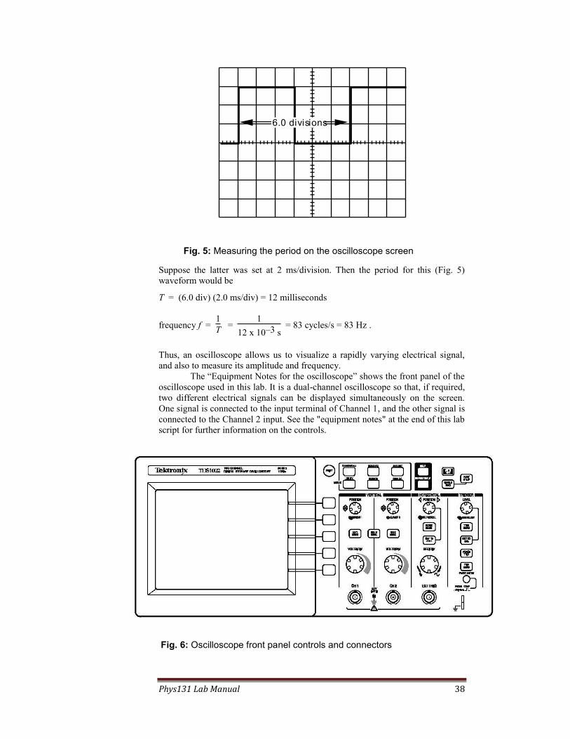
Phys131 Lab Manual 38
Suppose the latter was set at 2 ms/division. Then the period for this (Fig. 5)
waveform would be
T = (6.0 div) (2.0 ms/div) = 12 milliseconds
frequency f = 1
T =
1
12 x 10–3 s = 83 cycles/s = 83 Hz .
Thus, an oscilloscope allows us to visualize a rapidly varying electrical signal,
and also to measure its amplitude and frequency.
The “Equipment Notes for the oscilloscope” shows the front panel of the
oscilloscope used in this lab. It is a dual-channel oscilloscope so that, if required,
two different electrical signals can be displayed simultaneously on the screen.
One signal is connected to the input terminal of Channel 1, and the other signal is
connected to the Channel 2 input. See the "equipment notes" at the end of this lab
script for further information on the controls.
6.0 divisions
Fig. 5: Measuring the period on the oscilloscope screen
Fig. 6: Oscilloscope front panel controls and connectors

Phys131 Lab Manual 39
Important!
The oscilloscope (and most electronic equipment) is supplied with a 3-pin AC
plug for safety. The chassis (i.e., the part you can touch) is always grounded to
the round ground pin of the AC plug, which goes to earth ground. The shields of
both CH1 and CH2 inputs are both grounded to the oscilloscope's chassis and
earth ground as well. Thus the grounds of both channels are electrically
connected together and you must be careful to ground both channels at the same
point in your circuits;, otherwise, you will short out circuit elements. The
electrical grounds of any other instruments must also be connected to the same
ground point unless you know that the instrument has a "floating ground," i.e., a
negative terminal not connected to the instrument's chassis and to earth ground.
C. Probes
Oscilloscope probes
are recommended for
many measurements because they provide several useful features:
1. They have a little clip that can be hooked on to bare wires in a circuit. The clip
can be slipped off to expose a pointed tip that can probe small electrical contacts.
2. There is another clip for attaching to a ground point in the circuit being
measured.
3. Most probes are “times-ten” (10X) probes and increase the input impedance of
the oscilloscope by a factor of 10. This increase of the input impedance means
that the act of making a measurement has less effect on the circuit’s operation. If
the scope has a 1 MΩ input impedance, using a 10X probe would increase that to
10 MΩ. If you were measuring the voltage across a 1 MΩ resistor, connecting the
scope without a 10X probe would decrease the voltage to half its value. Using a
10X probe would only decrease its value by one-tenth. There is also a
compensation adjustment that can eliminate the effect of the small input
capacitance of the oscilloscope (i.e., the imaginary part of its input impedance)
which can cause the shape of the input signal to be distorted.
The 10X probe provides the oscilloscope input with only 1/10 of the
voltage it is measuring. One must compensate when reading the value. There is a
setting under the “vertical menu” that will automatically adjust for the use of a
probe. On startup, it assumes that measurements are made with a 10X probe and
multiplies measurements by 10 and the vertical V/div value by1/10 before
displaying them.
Experiment
I. Measuring the internal calibration signal (PROBE COMP) and using the Vertical Menu
(a) Attach a probe to the CH1 input and connect it to the calibration signal which
is labelled “PROBE COMP”. The ground clip should be clipped to the bottom tab
of the signal output, and the probe hook should be hooked on the top part.
(b) Slide the 1X/10X switch on the probe to 10X.
(c) Press the Autoset button. The scope attempts to find the best settings to
display the signal
Fig 7: Connecting the probe to the internal calibration signal.

Phys131 Lab Manual 40
You should now see a “square wave” signal on the screen: .
If the signal looks like this or like this , then the
compensation of the probe needs adjusting. The adjustment requires a special
little screwdriver; ask an instructor or a technician to do it.
(d) Find the following information on the screen display:
Vertical V/div scale
Horizontal sec/div scale
Number of vertical divisions between bottom and top of signal
Number of horizontal divisions in one complete period
From these values, you can calculate the peak-to-peak amplitude and frequency
of the signal. The readout also displays measurements of these values, thus
obviating the need to actually think about what you’re doing. Find these values
Peak-to-peak amplitude of the signal
Frequency of the signal
Compare with the values you got by calculating.
A little 1 on the left-hand side of the screen shows the zero voltage level for
channel 1. A little arrow on the right-hand side shows the trigger voltage and a
downward pointing arrow on the top shows the trigger point. Try to find these
features.
(e) Turn the Volts/div know above CH1 a few click clockwise and
counterclockwise. Attempt to understand the display changes that these
adjustments cause.
Try adjusting the position knobs, too. Notice that the little “1” on the
left-hand side of the screen moves as you change the position knob for CH1.
(f) Similarly, turn the sec/div scale clockwise and counterclockwise. Observe
what happens to the signal’s display. Can you understand what happens?
(g) Press the CH1 MENU button. The Vertical Menu is displayed beside the
signal display. From top to bottom, the following options can be adjusted by
pressing the button beside them:
Input Coupling: DC/AC/GND. Change to AC and observe the change. The
signal is now centred about the zero-volt level. On AC, a high-pass filter
takes out the DC component and reduces the low frequency components of
the signal. On GND, the signal is zero. Normally, one uses DC coupling
unless it’s necessary to suppress a large DC offset in the signal.
a
a
a
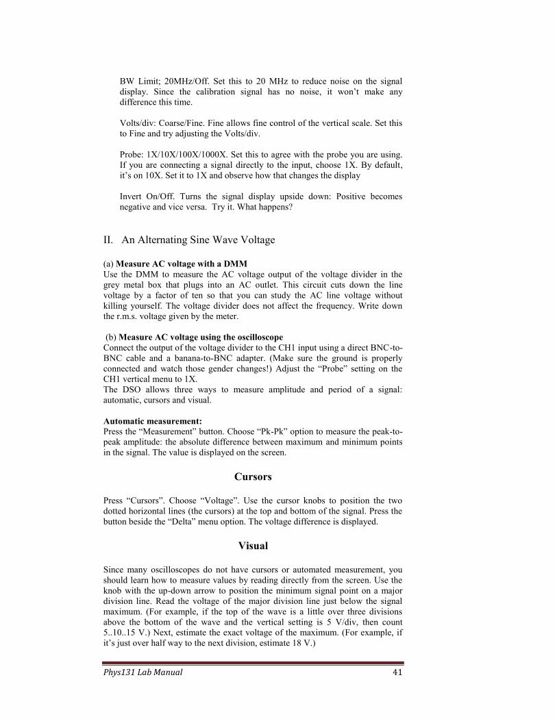
Phys131 Lab Manual 41
BW Limit; 20MHz/Off. Set this to 20 MHz to reduce noise on the signal
display. Since the calibration signal has no noise, it won’t make any
difference this time.
Volts/div: Coarse/Fine. Fine allows fine control of the vertical scale. Set this
to Fine and try adjusting the Volts/div.
Probe: 1X/10X/100X/1000X. Set this to agree with the probe you are using.
If you are connecting a signal directly to the input, choose 1X. By default,
it’s on 10X. Set it to 1X and observe how that changes the display
Invert On/Off. Turns the signal display upside down: Positive becomes
negative and vice versa. Try it. What happens?
II. An Alternating Sine Wave Voltage
(a) Measure AC voltage with a DMM
Use the DMM to measure the AC voltage output of the voltage divider in the
grey metal box that plugs into an AC outlet. This circuit cuts down the line
voltage by a factor of ten so that you can study the AC line voltage without
killing yourself. The voltage divider does not affect the frequency. Write down
the r.m.s. voltage given by the meter.
(b) Measure AC voltage using the oscilloscope
Connect the output of the voltage divider to the CH1 input using a direct BNC-to-
BNC cable and a banana-to-BNC adapter. (Make sure the ground is properly
connected and watch those gender changes!) Adjust the “Probe” setting on the
CH1 vertical menu to 1X.
The DSO allows three ways to measure amplitude and period of a signal:
automatic, cursors and visual.
Automatic measurement:
Press the “Measurement” button. Choose “Pk-Pk” option to measure the peak-to-
peak amplitude: the absolute difference between maximum and minimum points
in the signal. The value is displayed on the screen.
Cursors
Press “Cursors”. Choose “Voltage”. Use the cursor knobs to position the two
dotted horizontal lines (the cursors) at the top and bottom of the signal. Press the
button beside the “Delta” menu option. The voltage difference is displayed.
Visual
Since many oscilloscopes do not have cursors or automated measurement, you
should learn how to measure values by reading directly from the screen. Use the
knob with the up-down arrow to position the minimum signal point on a major
division line. Read the voltage of the major division line just below the signal
maximum. (For example, if the top of the wave is a little over three divisions
above the bottom of the wave and the vertical setting is 5 V/div, then count
5..10..15 V.) Next, estimate the exact voltage of the maximum. (For example, if
it’s just over half way to the next division, estimate 18 V.)

Phys131 Lab Manual 42
The period of the signal can be estimated the same three ways and the
frequency is just 1/period in each case. Direct measurement of the frequency is
also available under the “Measurement” menu.
Measure both the peak-to-peak amplitude and the period using the three
ways explained above. Compare the measurements to each other and to the value
from the DMM.
Accuracy:
The claimed vertical scale calibration accuracy is ±3% (for the 5 V/div to
10 mV/div scales) or ±4% (2 mV/div or 5 mV/div). The probe’s 10:1
attenuation is accurate to ±2%. So there is about ±5% possible error on most
voltage measurements. In addition, the analog-to-digital converter has eight
bits, which means the full scale is divided into 256 bins. One should allow
for a ±1 bin conversion error so that there is a possible digitization error
given by the V/div setting multiplied by 8/256 = 1/32. (Because there are
eight vertical divisions over the scope range.) Example: you are reading
V=10.2 V on the 5V/div scale. From the calibration accuracy we get
±5%x10V = ±0.5 V. From digitization accuracy using the 5V/division scale
we get: ±5V/32 = ±0.2 V. Combining gives a generous ±0.7 V possible
error.
The time base can be considered to be calibrated accurately (digital
clocks lose less than 1s per day), but the digitization rate is 250 sample bins
per major time division on the oscilloscope. You should allow at least ±1
bin error on any time measurement. For example if you read a time of 1 ms
on while on the 0.2 ms/div scale that would imply ±0.2 ms/250 or ±0.4 µs
error due to digitization. Of course, if the actual points marking the time
interval are uncertain, then that should be included in the error estimate as
well.
III. Examining the charge and discharge of a capacitor
Now investigate the relationship between the input and output of a circuit with
both a resistor R and capacitor C, with the output being taken across the
capacitor. This circuit is similar to the RC circuit of the DC circuits lab, except
that the function generator switches between charging and discharging the
capacitor.
Read the resistance and capacitance values and calculate the time
constant, RC. The resistor and capacitor values are approximately R = 10.0
kΩ and C is between 0.01 and 0.10 µF. Set the function generator to the square
wave output, and select a frequency whose period is many times longer than .
Connect the above circuit. The signal from the function generator (Vin)
should be connected to CH1, and the output signal across the capacitor (Vout)
connected to CH2. Turn on the function generator, and adjust the oscilloscope so
that you can see the signals from both channels. You should see an exponential
rising and falling of the output signal on channel 2 synchronized with the square
wave of channel one. Trigger SOURCE should be on CH1
Note: Be careful to connect the grounded (black) terminals of the
oscilloscope inputs to the same point in the circuit. Make sure you use
the same output from the function generator to feed both Ch. 1 input and
the filter.

Phys131 Lab Manual 43
(a) Measure the RC time constant. Adjust the function generator peak-to-
peak output voltage to a convenient voltage, V0 and its period to be several
times RC. The peak-to-peak output voltage across the capacitor should also
be about V0. If it is less, you probably need to decrease the frequency. Use
the oscilloscope to measure the time it takes the voltage on the capacitor to
fall from V0 to V
0/e. This measured time is the time constant τ. For
convenience, you may choose V0 = 2.71 V. Then V
0/e = 1 V.
(b) Observe square wave filter output near the cutoff frequency. Increase
the frequency of the function generator so that the period is about RC.
Sketch the waveform across the capacitor, indicating the time and voltage
scales.
(c) Observe square wave filter output at high frequencies. Increase the
frequency further until RC is many times the period. Sketch the output and
note the relative magnitudes of the input and output voltages.
Use the capacitor charging and discharging model to explain in a brief
sentence why the relative output voltage is nearly the same as the input voltage at
frequencies much less than 1/τ but diminishes to zero as the frequency increases
above 1/τ.
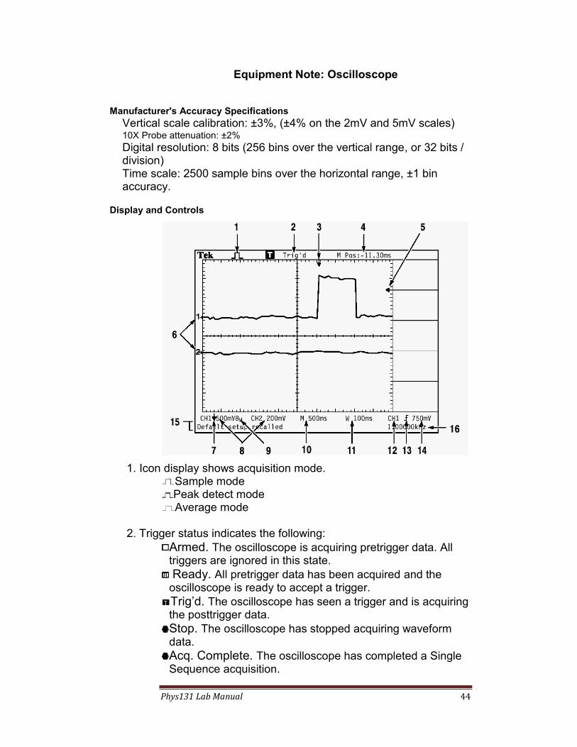
Phys131 Lab Manual 44
Equipment Note: Oscilloscope
Manufacturer's Accuracy Specifications
Vertical scale calibration: ±3%, (±4% on the 2mV and 5mV scales) 10X Probe attenuation: ±2%
Digital resolution: 8 bits (256 bins over the vertical range, or 32 bits / division) Time scale: 2500 sample bins over the horizontal range, ±1 bin accuracy.
Display and Controls
1. Icon display shows acquisition mode. Sample mode Peak detect mode Average mode
2. Trigger status indicates the following:
Armed. The oscilloscope is acquiring pretrigger data. All triggers are ignored in this state. Ready. All pretrigger data has been acquired and the oscilloscope is ready to accept a trigger.
Trig’d. The oscilloscope has seen a trigger and is acquiring the posttrigger data.
Stop. The oscilloscope has stopped acquiring waveform data.
Acq. Complete. The oscilloscope has completed a Single Sequence acquisition.
a
a

Phys131 Lab Manual 45
R Auto. The oscilloscope is in auto mode and is acquiring waveforms in the absence of triggers.
Scan. The oscilloscope is acquiring and displaying waveform data continuously in scan mode.
3. Marker shows horizontal trigger position. Turn the HORIZONTAL POSITION knob to adjust the position of the marker. 4. Readout shows the time at the center graticule. The trigger time is zero. 5. Marker shows Edge or Pulse Width trigger level. 6. On-screen markers show the ground reference points of the displayed waveforms. If there is no marker, the channel is not displayed.
7. An arrow icon indicates that the waveform is inverted. 8. Readouts show the vertical scale factors of the channels. 9. A BW icon indicates that the channel is bandwidth limited. 10. Readout shows main time base setting. 11. Readout shows window time base setting if it is in use. 12. Readout shows trigger source used for triggering. 13. Icon shows selected trigger type as follows:
-- Edge trigger for the rising edge. -- Edge trigger for the falling edge. -- Video trigger for line sync. -- Video trigger for field sync. -- Pulse Width trigger, positive polarity. -- Pulse Width trigger, negative polarity.
14. Readout shows Edge or Pulse Width trigger level. 15.Display area shows helpful messages; some messages display for only three seconds. If you recall a saved waveform, readout shows information about the reference waveform, such as RefA 1.00V 500µs. 16. Readout shows trigger frequency.
Control Function
AUTOSET Automatically adjusts settings to display the input signals
VOLTS/DIV Changes the vertical voltage scale
SEC/DIV Changes the horizontal time scale
CH1 MENU
Displays a menu of settings which affect the voltage display for Channel 1.
Input coupling: AC/DC/GND Bandwidth limit: 20 MHz/off V/div control fineness: Coarse/Fine Probe attenuation: 1X, 10X, 100X, 1000X Inversion: Off/On
Option Buttons Chooses the menu item directly to its left

Phys131 Lab Manual 46
MEASUREMENT Displays the measurement menu:
Freq, Period Mean, Pk-Pk, Cyc RMS, Min, Max, Rise Time, Fall Time, Pos Width, Neg Width and None.
POSITION Three knobs which control the up-down position for CH1 and Ch2 and
the left-right position for both channels. The CH1 and CH1 position
function as cursor position controls when the Cursor menu is active.
CURSOR Displays a menu allowing cursor readings: Type (Voltage, Time),
Source (Ch1, Ch2) Delta, Cursor1, Cursor2
DISPLAY Gives a menu controlling how the display works:
Type (vectors, dots), Persist (off,1s,2s..infinite), Format (YT,XY),
Contrast lighten/darken
TRIGGERING
TRIGGER LEVEL Sets the voltage level at which the signal display is fixed to the trigger
point on the screen.
TRIG MENU
SOURCE: CH1: Triggered from signal on CH1 CH2: Triggered from signal on CH2 EXT: Triggers on signal applied to the EXT TRIG input. AC LINE: Triggers on 60 Hz line frequency. (or 50Hz)
SLOPE:
Rising: Trigger level set at a rising voltage, pos slope Falling: Trigger level set at a falling voltage, neg slope
MODE: AUTO: Triggered sweep if trigger signal is present, Free runs if no trigger is present. NORM: Triggered sweep. No trace displayed if trigger is absent
SET TO 50% Sets the trigger level to half way between the signal max and min. .
Input and Output Connectors
Connector Function
CH1, CH2 These jacks connect the input signal to the respective vertical
amplifiers. Grounds go directly to scope's chassis and earth gnd.
EXT TRIG Connects a trigger signal that is independent of CH1 and CH2.
PROB COMP A square wave of 5 V peak-to-peak at 1 kHz is provided to allow for
the checking of the calibration of the Vertical channels and for
adjusting 10X probe compensation.
(Below PROBE COMP) Another ground connection to scope chassis and earth ground.

Phys131 Lab Manual 47
Equipment Note: BNC to Banana Plug Adapter
The coaxial cables in the lab have BNC
type connectors. The outer shield of the
coaxial cable and of the BNC connector
is ground. There are several types of
adapters to change from BNC connectors
to unshielded wires with banana plugs.
These adapters usually have a tab to
indicate which banana plug goes to
ground. The converters also have holes
for cascading multiple banana plug
connections. This diagram shows the
female-BNC to male-banana version.
Equipment Note: Function Generator
Like the oscilloscope, the function generator will be used in a number of different experiments,
so you should become familiar with the controls. Most of our function generators have a control
panel as shown.
The frequency generator is shown adjusted to give a 1 kHz sine wave.
FREQUENCY frequency = dial setting x multiplier range
AMPLITUDE Varies peak-to-peak voltage of output
OUTPUT Use the output jack on the upper right
OFFSET Allows DC offset to be added to the AC signal
DUTY Changes the duty cycle or symmetry of output waveform
(fully counterclockwise on CAL gives a 50% duty cycle)
FREQUENCY READOUT Updated once every counting period as signaled by GATE light.
Tab
Outside shield is ground
Banana Plug on
tab side is
ground
Middle conductor
inside BNC
connector is signal
1M 100k 10k 1k 100 10 1
?0dB ?0dBTTL/CMOS OUTPUT
EXT ?0dB
COUNTER ATTENUATOR
EXT COUNTER VCF
MIN MAX
AMPLITUDEPUSH TTLOFFSETDUTYRATEWIDTHFREQUENCY
0.2 2SWEEP
0.1s 10s0.01s 1sKENWOOD FUNCTION
GENERATOR
ON OFFPOWER
kHz
1.000
Frequency Ranges
Frequency Counting Periods
Adjust FrequencyConnect Output
Here
Choose Waveform (Sinewave)
This knob should be pushed in
Adjust for Desired Amplitude
0.2 to 2 kHz range
CAL

Phys131 Lab Manual 48
Prelab Questions
1. In Part II a voltage divider is used to decrease standard line voltage to a

Phys131 Lab Manual 49
Lab 4 – The Magnetic Field
References
Tipler (6th ed.): 26-1,2; 27-2,4.
Halliday, Resnick and Krane, (5th Ed.): 32-5; 33-4.
Objectives
I. To trace the magnetic field of a permanent magnet.
II. To create a magnetic field with an electric current.
III. To investigate the force on a moving charge in a magnetic field and to
measure this force using the current balance.
IV. To create an electric field with a changing magnetic field.
Apparatus
Permanent bar magnet
Compass
Large sheet of white paper for field tracing
Galvanometer frame
Solenoid with current balance attachment, weights
Cathode Ray Oscilloscope
Ammeter
Introduction
Magnetic Fields In the first part of this experiment, you will investigate the magnetic field
of a bar magnet. The direction of the magnetic field is the direction of the force
on a north magnetic monopole if it was placed in a magnetic field. A north
magnetic monopole is a magnet with only a north pole. Unfortunately, none have
ever been found to exist, so we'll have to make do with something else: a
compass. If we place a compass in a magnetic field, its north pole points in the
direction of the magnetic field. Figure 1 illustrates the magnetic field of the Earth.
Forces on Currents in Magnetic Fields
Suppose you place a loose wire in a uniform magnetic field. (See Fig. 2.)
The field may be either the field of a permanent magnet or the field produced by
a current that we control. If no current flows through the wire, it will droop under
the force of gravity. When current passes through the wire, the wire is pushed
across the magnetic field. A number of experiments can establish the rules
describing the force produced by a magnetic field on a current.

Phys131 Lab Manual 50
Fig. 1: (a) The Earth seems to have a gigantic bar magnet embedded in it with a South pole in the northern hemisphere. (b) The field lines show the direction of the horizontal component of the magnetic field on the Earth’s surface. (c) The complete field map reveals that there is a significant vertical component to the Earth’s magnetic field at most places. (From Physics for the Inquiring Mind, E. Rogers, Princeton University Press, 1960.)
(i) The force is perpendicular to both the magnetic field and the current. If
your nose points in the direction of the field and a current passes from
left to right across your field of vision, the force will be upwards.
Another way to describe the direction is to stretch out your right hand.
Your fingers point in the direction of the field; your thumb in the
direction of the current; and the force will point straight outwards from
the palm of your hand.
(ii) By changing the strength of the field without changing its direction we
find that the force is proportional to the magnitude of the field. By
changing the direction of the field without changing its magnitude we
find that only B, the field component perpendicular to the wire,
contributes to the force. Therefore, the force is proportional to B, the
magnitude of the perpendicular component of the magnetic field.
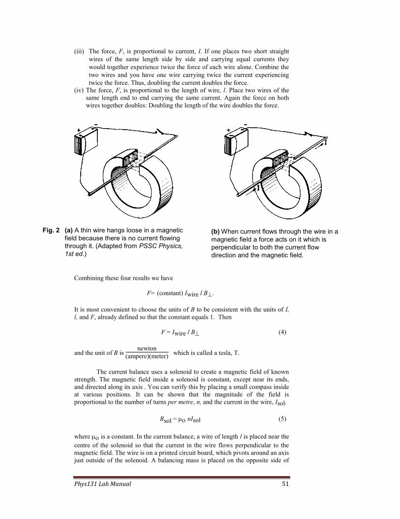
Phys131 Lab Manual 51
(iii) The force, F, is proportional to current, I. If one places two short straight
wires of the same length side by side and carrying equal currents they
would together experience twice the force of each wire alone. Combine the
two wires and you have one wire carrying twice the current experiencing
twice the force. Thus, doubling the current doubles the force.
(iv) The force, F, is proportional to the length of wire, l. Place two wires of the
same length end to end carrying the same current. Again the force on both
wires together doubles: Doubling the length of the wire doubles the force.
Fig. 2 (a) A thin wire hangs loose in a magnetic
field because there is no current flowing
through it. (Adapted from PSSC Physics,
1st ed.)
(b) When current flows through the wire in a
magnetic field a force acts on it which is
perpendicular to both the current flow
direction and the magnetic field.
Combining these four results we have
F= (constant) Iwire l B.
It is most convenient to choose the units of B to be consistent with the units of I,
l, and F, already defined so that the constant equals 1. Then
F = Iwire l B (4)
and the unit of B is newton
(ampere)(meter) which is called a tesla, T.
The current balance uses a solenoid to create a magnetic field of known
strength. The magnetic field inside a solenoid is constant, except near its ends,
and directed along its axis . You can verify this by placing a small compass inside
at various positions. It can be shown that the magnitude of the field is
proportional to the number of turns per metre, n, and the current in the wire, Isol.
Bsol = nIsol (5)
where is a constant. In the current balance, a wire of length l is placed near the
centre of the solenoid so that the current in the wire flows perpendicular to the
magnetic field. The wire is on a printed circuit board, which pivots around an axis
just outside of the solenoid. A balancing mass is placed on the opposite side of

Phys131 Lab Manual 52
the pivot point to the wire. If the arms of the balance are of equal length and the
forces balance, then
Fmagnetic = Fgravity
Iwire lBsol = mg
Fig 3: How to “weigh” the magnetic field.
Solving for Bsol
Bsol= mg
Iwire l (6)
Therefore, we can measure the magnetic field in the solenoid by measuring the
force on a wire of length l in the field carrying a current Iwire which is at right
angles to the field.
Fig. 4: The current balance consists of a current-carrying conductor on a
balance arm inside a solenoid. The magnetic field of the solenoid is
perpendicular to the direction of current flow at the end of the arm.
Induced EMF Put a loop of wire in a uniform magnetic field. Let A represent the area
encircled by the wire and B the component of the magnetic field perpendicular
to the surface enclosed by the wire. The quantity AB is called the magnetic flux,
AB by definition.
The units of magnetic flux are Webers which are equivalent to Tm2 or Nm/A.
This definition of flux will prove useful in describing the EMF induced by
magnetic fields.
Please Note: In this experiment, you will measure magnetic fields. When doing
so, you must keep all other sources of magnetic fields, mainly magnets but also
current-carrying wires, away from the area where you are making measurements.
Another magnetic field in your working area is the earth's. It is small but
mgI l Bsolwire
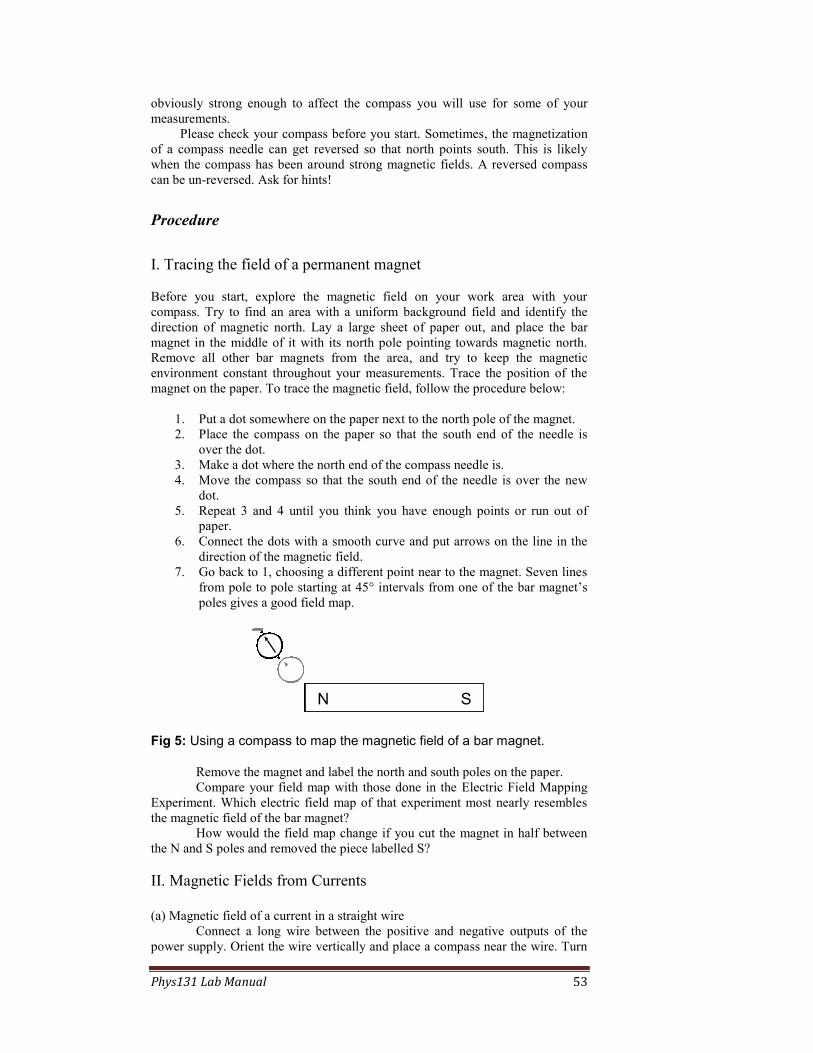
Phys131 Lab Manual 53
obviously strong enough to affect the compass you will use for some of your
measurements.
Please check your compass before you start. Sometimes, the magnetization
of a compass needle can get reversed so that north points south. This is likely
when the compass has been around strong magnetic fields. A reversed compass
can be un-reversed. Ask for hints!
Procedure
I. Tracing the field of a permanent magnet
Before you start, explore the magnetic field on your work area with your
compass. Try to find an area with a uniform background field and identify the
direction of magnetic north. Lay a large sheet of paper out, and place the bar
magnet in the middle of it with its north pole pointing towards magnetic north.
Remove all other bar magnets from the area, and try to keep the magnetic
environment constant throughout your measurements. Trace the position of the
magnet on the paper. To trace the magnetic field, follow the procedure below:
1. Put a dot somewhere on the paper next to the north pole of the magnet.
2. Place the compass on the paper so that the south end of the needle is
over the dot.
3. Make a dot where the north end of the compass needle is.
4. Move the compass so that the south end of the needle is over the new
dot.
5. Repeat 3 and 4 until you think you have enough points or run out of
paper.
6. Connect the dots with a smooth curve and put arrows on the line in the
direction of the magnetic field.
7. Go back to 1, choosing a different point near to the magnet. Seven lines
from pole to pole starting at 45° intervals from one of the bar magnet’s
poles gives a good field map.
Fig 5: Using a compass to map the magnetic field of a bar magnet.
Remove the magnet and label the north and south poles on the paper.
Compare your field map with those done in the Electric Field Mapping
Experiment. Which electric field map of that experiment most nearly resembles
the magnetic field of the bar magnet?
How would the field map change if you cut the magnet in half between
the N and S poles and removed the piece labelled S?
II. Magnetic Fields from Currents
(a) Magnetic field of a current in a straight wire
Connect a long wire between the positive and negative outputs of the
power supply. Orient the wire vertically and place a compass near the wire. Turn
N S

Phys131 Lab Manual 54
on a current of more than 2 amps. Describe what happens to the compass needle
as you switch the current on and switch it off. Try the compass at various posi-
tions around the wire.
(b) Magnetic field of a current loop
Take the galvanometer frame (the set of loops of wire on a plastic frame)
and orient it so that the wires point in a north-south direction. Connect a power to
the single loop and run a current of 1 to 2 ampères through it.
Use the “current source” mode of the power supply:
•Initially, the Voltage setting should be higher than zero and the Current set at
zero (totally counterclockwise).
•Start to raise the current very slowly by gently turning the current knob
clockwise.
•Look at the power supply’s ammeter to measure the current.
•If the current reaches a plateau and doesn’t increase as you turn the current
knob clockwise, then the voltage setting is too low and needs to be
increased a little.
Investigate the magnetic field around the loop using the compass.
Compare the field map of the bar magnet with what you observe for the coil.
Now place the compass in the loop so that the needle is directly under the
wire. At first, when there is no current, the needle should be aligned parallel to
the wire. Vary the current through the loop while watching the compass needle
start to turn. Increase the current until the needle points 45˚ from north (either
northeast or northwest). Record this current. The compass is under the influence
of two magnetic fields: the Earth's, pointing north (more or less), and the current
loop's, pointing east or west. When the compass is at 45˚, the two fields have
equal magnitude.
Next, place the compass under the 20-turn loop, and align the needle
with the wire, as before. Run current through the set of 20 loops, and find how
much current needed to move the compass to 45˚. The current is now much
smaller, and the ammeter is less accurate at these levels. Nevertheless, you should
be able to see the expected relationship of magnetic field, B, to the number of
loops, N, and the current, I.
Fig 6: The magnetic fields of a coil of wire and the earth add like vectors.
III. Force on a Moving Charge in a Magnetic Field
(a) Moving electrons in a cathode ray oscilloscope
Cathode ray oscilloscopes have an electron beam, which travels from the
rear to the front, to produce an image on the fluorescent screen. There are cathode
ray oscilloscopes in the lab for this experiment. Reduce the intensity knob
NI1 I2
B of earth
B f rom coil
resultant B

Phys131 Lab Manual 55
completely counterclockwise. Turn on the oscilloscope, and place the Horiz
Mode switch on XY. Increase the intensity until you see a spot on the screen.
Using the vertical and horizontal position dials, centre the dot on the screen.
Keep the intensity low so the electron beam doesn’t damage the screen and
turn it off immediately after you finish.
Use your field map of the bar magnet to help you orient the bar magnet
horizontally in front of the oscilloscope screen so that B is perpendicular to the
electron velocity with N on the left, S on the right. Slowly move the bar magnet
towards the screen in this orientation, and sketch the relative directions of B, v,
and F, as measured by the beam’s deflection. Reverse the direction of B (N on
the right), and again sketch the B, v, and F directions.
From these observations, devise your own “rule” to help you remember
the direction of the force on an electron moving in a magnetic field. Use your rule
to predict the deflection of the beam when the bar magnet is held vertically near
the screen with N on top, then S on top. Try it to test the prediction.
(b) The Current Balance: “Weighing” a magnetic field
Mount the current balance arm in the solenoid as shown in Fig. 7. Orient
the balance so that the Earth's field runs parallel to the wire on which we are
going to measure the force. The current within that section of wire will then feel
no net force from the Earth's field. It may help to clean the pivoting contact with
a piece of sandpaper to insure good electrical contact
Connect the power as shown. The switch and ammeter are those internal
to the power supply. Note that in this case we use the same current through the
solenoid and through the wire on the balance arm. (It would be better to have
independent current supplies for the solenoid and the current balance arm. In
order to have two independent currents, work with another group so that you can
use two power supplies. The circuit must then be changed accordingly.)
Fig. 7: Connect the current from one power supply so that it goes through both the
solenoid and the balance arm in series.

Phys131 Lab Manual 56
Clip a (non magnetic) paper clip on the arm of the balance at a position
such that the arm is balanced horizontally when no current is flowing.
Fold a file card so that you can stand it next to the balance and mark the
“balance” position with a tick mark.
Make sure that the balance is swinging reasonably freely by setting it
swinging. If it stops within a second, there's too much friction; check to see
whether the balance rubs against the sides of the solenoid. Place small masses on
the outside end of the balance arm at a distance from the pivot equal to that of the
current-carrying wire, which is perpendicular to B on the arm in the solenoid.
Increase the current until the arm comes back to its balance position. Add mass
(small plastic washers), each time measuring the current needed to balance the
swinging arm. (Note: The mass of a small plastic washer is comparable to the
balance resolution which is 0.01g. How can you minimize the uncertainty in this
measurement?)
For each value of m and Iwire, calculate Bsol from equation (6). The
value of n for your solenoid should be marked on it. Plotting Bsol vs. Isoln should
give a straight line with slope . Alternatively, you can calculate for each
data pair. The second method is equivalent to forcing through the origin the
straight line of the Bsol vs. Isoln graph. This might not be justified if there is a
systematic error in the data resulting in a nonzero intercept. Do your data indicate
such a systematic error?
IV. Induced EMF (qualitative) (Optional)
(a) Induction with a bar magnet and loop
Remove the current balance attachment and all wires from the solenoid.
Hook the solenoid up to the oscilloscope. Set the time/div scale on the oscillo-
scope to 0.1 ms/div. Take the bar magnet and bring its north pole near to the
solenoid. Quickly push the magnet into the solenoid, watching the trace on the
oscilloscope screen. If you don't see anything, increase the sensitivity of the
voltage setting and adjust the trigger setting. Sketch the approximate shape of the
scope trace, making sure to record the V/div setting. Pull the magnet out of the
solenoid, once more sketching the oscilloscope response. Repeat the above
procedure with the south pole of the magnet, and on the other side of the
solenoid. Sketch the apparatus, making sure to note the sense of the current in the
solenoid.
Do the same for a single loop of wire and for multiple loops, which you
can make yourself by wrapping wire around a suitable form. Try to keep the
speed at which you move the magnet the same for both. Which creates a larger
voltage: the single loop or multiple loops? How many times larger does it appear
to be? Compare what happens when you move the loop instead of the magnet.
Fig. 8: Changing the magnitude of the field through a loop of wire by
NN S
to oscilloscope input
mov e back and f orth
N S
to oscilloscope input
mov e back and f orth
NN S
to oscilloscope input
N S
to oscilloscope input
twist

Phys131 Lab Manual 57
moving the bar magnet back and forth and changing its direction by twisting the bar magnet.
Can you find any induced EMF in the loop for the following
experiments? How does the rate of the changes affect the size of the EMF?
•Bring the north or south pole of the magnet close to the centre of the
loop. Quickly twist the bar magnet so the direction that the field passes through
the loop changes, but the magnitude of the field stays about the same at the centre
of the coil. (Refer to your bar magnet field map.)
•Hold the magnet close to the loop, and quickly reduce the loop’s area by
tightening it like a noose. You may try to thread the wire through a washer or
similar device to aid this attempt.
Summarize your findings about the induced EMF caused by the following
factors:
1. rate of change in the magnitude of magnetic field passing through a
loop;
2. rate of change of the direction of the magnetic field passing through a
loop;
3. rate of change of the area of loop with magnetic field passing through it;
4. number of loops.
Show that a formula involving the flux can encapsulate all these results.
(b) Inducing AC signals using a solenoid
Connect the function generator to the solenoid, and drive an AC signal of
about 1000 Hz through it. Choose the sinusoidal waveform. Monitor the AC
signal from the function generator on Ch1 of the oscilloscope. Connect a long
plain wire between the signal input and ground input of Ch2. You may need to
use a coaxial cable to take the signal picked up from the test loop to the
oscilloscope input. This helps eliminate noise pickup when you are viewing small
voltage signals.
Wrap the wire around the solenoid, and adjust the scope to see whether
you can pick up the signal from the solenoid.
Try the following experiments:
1. Compare the signal strength picked up by one loop around the solenoid
when the frequency generator is at 500 Hz, 1000 Hz and 2000 Hz. (Keep
other parameters, such as loop size, the same.)
2. Compare the signal strength picked up by one loop wrapped tightly
around the solenoid to that picked up by a much larger diameter loop.
What happens when the loop does not encircle the solenoid?
3. Compare how the signal strength varies when the loop’s orientation with
respect to the magnetic field of the solenoid is changed: e.g., Surface
area encircled by the loop is normal to the magnetic field vs. at a 45°
angle.
4. Make a much smaller loop by wrapping the insulated hookup wire
around one finger. (approximately 1 cm diameter). Put the loops inside
the solenoid, oriented perpendicular to the magnetic field. Compare the
signal strength picked up to that picked up when the loop was encircling
the solenoid and outside it.
5. Tilt the loop at a 30° to 45° angle with respect to field. Is there any
difference in signal strength?
6. Double (or triple) the loop’s area by wrapping the wire around two (or
three) fingers. Insert the loop inside the solenoid, with the field
perpendicular to the loop. Compare the signal strength.
Phys131 Lab Manual 58
7. Switch the function generator from a sine to a triangle wave. Reduce the
frequency to around 250 Hz to reduce problems caused by the self-
inductance of the solenoid. Observe and explain the difference in the
induced waveform
Prelab Questions
1. A horizontal magnetic field B is perpendicular to the horizontal
component Be of the earth's magnetic field and points east.
(a) The ratio B/Be = 3 . In which direction will the compass needle
point? (The compass needle rotates in the horizontal plane and assume
Be points north.)
(b) If the compass needle points northwest, what is the magnitude of B?
2. The magnetic field inside a long solenoid is uniform and parallel to the
solenoid's axis. (See fig. 4.)
(a) What is the force on that portion of the current carrying wire inside
the solenoid that runs parallel to the solenoid's axis?
(b) The portion of the current carrying wire inside the solenoid that is
perpendicular to the axis is 2 cm long and carries 1 A current. The field
inside the solenoid is 1.0x10⁻² tesla. What is the force on the wire? How
much mass would it take to balance the force if it were placed at an
equal distance from the pivot?
(c) Describe how you would use this setup as an ammeter.
3. A solenoid is 2 cm in diameter and has 3720 turns/m. AC current with a
triangular waveform is passed through it. The current’s amplitude is 1 A
and frequency is 1 kHz. A circular loop of wire with a diameter of 1 cm
is placed inside the solenoid with the loop’s axis oriented parallel to the
solenoid’s. In theory, the flux through the loop is in phase with the
current’ and has the same waveform. On graph paper, graph the current
showing the current scale on the left-hand vertical axis and, on the right-
hand vertical axis, show a scale of the magnetic flux through the loop.
(See figure.)
Below this graph, show the graph of the induced EMF in the loop, which
is proportional to the time rate of change of the flux.
On the current graph, sketch another current waveform having the same
amplitude but double the frequency. (Use a dotted line or another
colour.)
On the EMF graph, sketch the EMF induced by the 2 kHz current.
Phys131 Lab Manual 59
Introduction to Optics
Equipments
Introduction
Our understanding of the world is largely determined by sight. How visual
sensations relate to material objects and how these sensations are transmitted is a
fascinating puzzle whose pieces have been assembled slowly through the
centuries. Our common understanding of the visual process has benefited from
efforts of scientists and philosophers of preceding generations. Even the least
scientifically educated person probably understands that the eyes passively
receive light reflected from objects and that light is produced by sources such as
the sun. This view is not self-evident. Ancient Greeks debated whether the eye
sends out “feelers” in order to see rather than passively receiving its sensations.
Observations and logic have long since refuted the “feeler” theory but other
debates have persisted. The relationship of the retinal image to the mind's visual
impression is still under investigation. More fundamentally, philosophers of
science are trying to reconcile the basic relationship of the observer to the
observed with recent findings of quantum physics.
Most naive observers intuitively understand light to be like a stream of
particles or like rays. This model accounts for many of our everyday experiences.
An elaborate particle theory of light flourished for many years under the
patronage of Sir Isaac Newton even though it failed to explain some easily
observed phenomena. The wave theory of Christian Huygens gained favour as
ever-more experiments showing interference effects gave results that disagreed
with expectations based on the particle theory. Later, the photoelectric effect was
discovered, and the wave theory had to be changed. What resulted was a wave-
particle model in which light particles, called photons, managed to retain many
wave-like properties. (Or should we say that light waves managed to acquire
particle properties!?)
As you experiment with light, you will try to understand what you see by
making analogies to things familiar in your previous experience: light acts like a
stream of pellets or like ripples in water. At first, these models help you
understand; later, they fall short. Finally, you should come to accept light in its
own right and realize that it is unlike anything else you know at all.
The following codes are used throughout the optics labs:
(E) Error analysis is required for this part.
(C) Less detailed instructions are given to encourage you to be creative.

Phys131 Lab Manual 60
Equipment Note: The Pasco Introductory Optics System
Figure 1 shows all the equipment in the OS-8500 Introductory Optics System.
The system also includes a fitted box with cutouts for each component.
Please replace all components in their places after each lab period before
returning the box.
Figure 1: Equipment included in the OS-8500 Introductory Optics System

Phys131 Lab Manual 61
Optics Bench
Figure 2: Using the optics Bench The optics bench is shown in Figure 2. The light source, component holders and ray table base all attach magnetically to the bench as shown. For proper optical alignment, the edge of each of these components should be mounted flush to the alignment rail which is the raised edge that runs along one side of the bench.
Note: Avoid scratching or otherwise abusing the surface of the magnetic pads. If they get dirty ask for them to be cleaned by the technician.
Incandescent Light Source
Figure 3: Using the light source
The light source is shown in Figure 3. To turn it on, connect the power cord
to any grounded 105-125 Vac receptacle, and flip the switch on the rear
panel to ON. If at any time the light fails to come on, check with your
instructor.
The filament knob on the top of the unit moves the light bulb from side
to side. The notch at the bottom indicates the position of the light bulb
filament, so that accurate measurements can be made during
experiments.

Phys131 Lab Manual 62
Component Holders
The optics set comes with three
regular component holders (Fig. 4)
and one holder designed for use
with the ray table. The regular
component holders attach
magnetically to the optics bench as
in Figure 5. The ray table holder sits
on the edge of the circular ray table.
The notch at the top of each holder
is for centring components on the
holder. The notches in the base of
the regular holders are for accurate
distance measurements on the
bench scale.
Figure 6: Component Alignment
Figure 5: Using The Component Holder

Phys131 Lab Manual 63
Lab 5 – RAY OPTICS, REFLECTION
AND CONCAVE MIRRORS
References
Tipler (6th ed.): 32-1: Mirrors.
Halliday, Resnick and Krane, (5th Ed.): 40-1,2,3.
Objectives (Suggested times in parentheses are approximate.)
I. Observe straight-line propagation of light. (15 min.)
II Locate an object by tracing rays. (30 min.)
III Study the law of reflection (45 min.)
IV Use ray tracing to locate a virtual images formed by a mirror (30 min.)
V Measure magnification and focal length of a cylindrical mirror (30 min.)
VI Form an image using a concave mirror and measure its magnification (30 min.)
VII Use the Virtual Image Locator to locate virtual images formed by mirrors. (30 min.)
Apparatus
From the Optics Kit: Optics Bench, Light Source, Ray Table and Base
Component Holders (2), Slit Plate, Ray Table Component Holder, Viewing
Screen, Concave Mirror, Virtual Image Locators, Ray Optics Mirror, Slit Plate.
Additional: 11x17 inch paper and a plane mirror
Fig. 1.1: Basic Ray Optics Setup

Phys131 Lab Manual 64
Introduction
Many useful properties of light can be understood in terms of a simple ray theory.
In these experiments, you will observe light as it travels through air of uniform
density. In this case, light propagates in a straight line from its source. One can
use a slit plate to select “rays” of light coming from a point source. These rays
can be traced back to their origin, where they cross at their source.
If light encounters a shiny surface, it undergoes specular reflection. Rays
reflect from mirrors according to the law of reflection: the angle of incidence
equals the angle of reflection where the angle is measured from the normal to the
reflecting surface. The rays reflected from a plane or convex mirror will not
cross, but if one extends them back in a straight line to the other side of the
mirror, these extensions will cross at a point called the virtual image of the
source. The virtual image is at the position from where the light appears to come.
In these experiments, we emphasize point sources because any object can be
considered as a collection of point sources. Therefore, the virtual image of any
object can be understood as a collection of virtual images of point light sources.
The law of reflection implies that the virtual image formed by a plane
mirror will be at the same distance from the mirror as the object, but on the other
side. If we form a virtual image using a concave mirror, then the law of reflection
tells us that the object-image distance is given by the following formula: 1
s
1
s
2
r
1
f
where s is the object-mirror distance, sis the image-mirror distance, r is the
mirror's radius of curvature and f is its focal length. The magnification of the
mirror is given by
m y
y –
s
s
where y and y are the image and object heights respectively. (See Tipler, 3rd
edition, p. 1016.)
When two objects are at different distances from an observer, the two
objects appear to move with respect to each other when the observer moves. This
visual phenomenon is called parallax. If two objects are at the same distance
from the observer, then there is no parallax. Images exhibit the same parallax as
objects. Therefore, if an object and a virtual image are at the same distance from
the observer, they will not move with respect to each other as the observation
point changes. Parallax can be used to locate virtual images and is the principle of
the Virtual Image Locators.

Phys131 Lab Manual 65
Fig. 1.2: Ray Tracing
Procedure
Part I - Preliminary Observations on Straight-Line Propagation
Set the equipment as shown in Fig 1.1. You may leave off the viewing screen at
first. Plug in the light source and turn it on. The bulb has a linear filament running
up and down.
1. Does light travel in a straight line from its source? Observe the rays that
emerge from the slit plate. Look at the rays on the ray table then lower your
head and peer along a ray. Are you sure that the rays do not bend as they
pass through the slits?
2. Find how to get sharp rays. Vary the distance between the slit plate and
the light source, and note how the width, brightness and sharpness of the
rays change. Observe how the distinctness and the direction of the rays
change as you rotate the slit plate so that the slits are not parallel with the
light bulb’s filament.
Summarize your findings of steps 1 and 2 using only a few sentences.
Part II - Locating the Filament (E)
Locate the position of the filament by tracing on a piece of paper the rays coming
through the slits. (E means do full error analysis.)
1. Mark the rays on the paper. Fold a piece of 11x17 inch paper in half to
make an 8.5x11 inch sheet. Tape the paper on the ray table with the fold
facing the filament and directly above the ray table base. Turn on the light,
and trace four rays that cross the paper.
Hint: If the rays are wide, it may be better to trace the edge of the rays.
You may mark two points of each ray before removing the paper.
Choose points that are widely separated for greater accuracy.
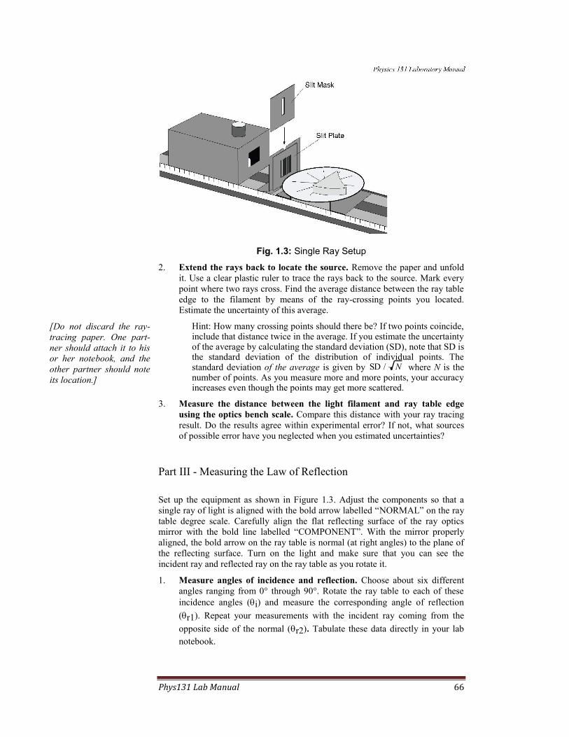
Phys131 Lab Manual 66
Fig. 1.3: Single Ray Setup
2. Extend the rays back to locate the source. Remove the paper and unfold
it. Use a clear plastic ruler to trace the rays back to the source. Mark every
point where two rays cross. Find the average distance between the ray table
edge to the filament by means of the ray-crossing points you located.
Estimate the uncertainty of this average.
Hint: How many crossing points should there be? If two points coincide, include that distance twice in the average. If you estimate the uncertainty of the average by calculating the standard deviation (SD), note that SD is the standard deviation of the distribution of individual points. The standard deviation of the average is given by SD / N where N is the number of points. As you measure more and more points, your accuracy increases even though the points may get more scattered.
3. Measure the distance between the light filament and ray table edge
using the optics bench scale. Compare this distance with your ray tracing
result. Do the results agree within experimental error? If not, what sources
of possible error have you neglected when you estimated uncertainties?
Part III - Measuring the Law of Reflection
Set up the equipment as shown in Figure 1.3. Adjust the components so that a
single ray of light is aligned with the bold arrow labelled “NORMAL” on the ray
table degree scale. Carefully align the flat reflecting surface of the ray optics
mirror with the bold line labelled “COMPONENT”. With the mirror properly
aligned, the bold arrow on the ray table is normal (at right angles) to the plane of
the reflecting surface. Turn on the light and make sure that you can see the
incident ray and reflected ray on the ray table as you rotate it.
1. Measure angles of incidence and reflection. Choose about six different
angles ranging from 0° through 90°. Rotate the ray table to each of these
incidence angles (i) and measure the corresponding angle of reflection
(r1). Repeat your measurements with the incident ray coming from the
opposite side of the normal (r2). Tabulate these data directly in your lab
notebook.
[Do not discard the ray-
tracing paper. One part-
ner should attach it to his
or her notebook, and the
other partner should note
its location.]

Phys131 Lab Manual 67
2. Analyze your data and determine the law of reflection. What criteria
must you use to determine whether your data agree with the law or not? Are
the results from the two trials the same? If not, why not?
Part of the law of reflection states that the incident ray, the reflected ray and
the normal to the reflecting surface lie in the same plane. Is this statement
consistent with your experiments?
Fig. 1.4: Alignment of the Ray Mirror for normal incidence and for incidence at an arbitrary angle

Phys131 Lab Manual 68
Part IV - Using Ray Tracing to Locate the Virtual Image (C)
In this part, you will use the method developed in part II to find the position of
the virtual image of a filament formed by a plane mirror. The basic idea is
illustrated in Figure 1.5. The (C) means that you may use your own ideas and be
creative in doing this part. Take notes clearly describing the procedure in your lab
notebook. Analyze the data and discuss the results. [Do not write on the ray
table.]
Part V - The Focal Length of a Concave Mirror
The image formed by a plane mirror is always virtual. A concave mirror can form
either a real image or a virtual image. A real image occurs if the rays come from a
distant source. If the source is closer than one focal length from the mirror, then a
virtual image is formed. If the source is exactly at the mirror’s focal point, the
rays emerge parallel from the mirror. This is the principle used in flashlights,
headlights and spotlights to produce a parallel beam of light.
Ideally, concave mirrors have a paraboloidal shape. Spherical shapes are
cheaper to manufacture than paraboloids, and most inexpensive concave mirrors
are spherical. For most applications, the loss in quality is insignificant,
particularly where the mirror’s f-number (focal length/diameter) is large. In the
following exercise, you will use the cylindrical ray optics mirror to visualize its
image-forming properties and find the mirror’s focal length by producing a
parallel beam of rays.
1. Mount the slit plate and ray table. Place the slit plate directly on the light
source and move the ray table so its edge touches it. Use the ray table
surface with a centimetre grid, and turn it so that the grid is aligned with the
optical bench axis.
2. Observe the real image formed by a concave mirror. Place the ray optics
mirror on the ray table; turn on the light; and observe the rays reflected from
the concave surface. When the mirror is at the far end of the table, you
should see the reflected rays converging at the position of the real image.
3. Rotate mirror to show aberration. If you turn the mirror so that the image
position is off the optical axis of the bench, you will notice that not all rays
converge at the same place. This is because the mirror’s shape is circular
instead of parabolic. This effect is known as spherical aberration when it
occurs in spherical mirrors.
4. Measure the source-mirror and image-mirror distances and
magnification. Orient the ray mirror so that the image is exactly on the
optic axis. Record the object-to-mirror distance, the image-to-mirror
distance. Slide the light source box a few mm away from the alignment rail,
keeping its edge
parallel to the rail.
Record the direction
and distance that
the image is
displaced for a
given light source
displacement. This
shows the
magnification and
inversion of the
image.

Phys131 Lab Manual 69
5. Find where the mirror gives parallel reflected rays. Slide the mirror
closer to the light source until the reflected rays diverge. The rays don’t
actually cross now, but their projections on the dark side of the mirror will
cross at the position of the virtual image. Move the mirror back until the
emerging rays are parallel. Measure the distance between the light source
and the mirror. Remove the mirror from the table, and have your partner
repeat this measurement to get two independent values for the focal
length
VI - Forming an Image with a Concave Mirror.
If you cut a strip along any diameter of a spherical mirror you get something
close to a cylindrical mirror. It's not surprising then that we can understand
spherical mirrors from the properties of cylindrical mirrors studied in the last
part.
1. Arrange components. Set up the equipment as shown in Fig 1.7 with the
concave side of the mirror facing the light source. The viewing screen
should cover only half of the hole in the component holder so that light
from the filament reaches the mirror.
2. Find focal point of a distant object. Estimate the focal length of the mirror
by positioning the mirror on the optical bench as far from the crossed arrow
target as possible. Vary the position of the viewing screen to find where the
image of the target is focussed. Record this approximate value of the focal
length and have your partner repeat the measurement independently.
Fig. 1.7: Setup to observe the image from a concave mirror
3. Measure object-mirror and image-mirror distances to get the Mirror's
focal length. Choose five distances between 500 mm and 50 mm. These are
object-mirror distances for which you will measure the image-mirror
distances and the image heights. Calculate f from s and sin each instance. Also, compare the magnification derived from y/y with that calculated from
s/s.

Phys131 Lab Manual 70
VII- Using the Virtual Image Locators (optional)
1. Find the virtual image formed by a plane mirror.
(a) Put one of the virtual image locators (VIL#1) on the near end of the optical
bench. Mount the plane mirror on a component holder so that it extends
above the holder’s top with the shiny side facing VIL#1 as in Fig. 1.8. Look
for the virtual image in the mirror.
(b) After seeing the image, put the second virtual image locator (VIL#2) near
where the image appears to be. When you sight down the optical bench axis,
you should see the image of the bottom half of the VIL#1 in the mirror at
the same time as you can see all of VIL#2 through the clear plastic of
VIL#1. When you look exactly down the axis, both arrows should coincide,
but you may observe parallax as you move your head left and right (or you
can move the bench right and left). Move the second virtual image nearer or
farther from you until the reflected image of VIL#1 shows no parallax with
VIL#2. The far virtual image locator is now at the position of the virtual
image formed by the plane mirror. Record the positions of the two virtual
image locators and the mirror in your notebook. Compare object and image
distances.
2.(C) Find the virtual image formed by a concave mirror. Use the same
principle to find the virtual image formed by the 50 mm f.l. concave mirror.
Develop your own method. Record the method and results in your notebook
Hints: Because the concave mirror’s mount is opaque, you may want to use a
straight edge to help align the images. You can mount the mirror sideways or

Phys131 Lab Manual 71
below the top of the component holder. In order to get the virtual image locator
within 50 mm of the mirror, you will need to orient the component holders so that
the short feet of the bases face each other. If the mirror’s axis is very slightly
misaligned with the optical bench axis, the virtual image will also be off axis. but
much more so. Don’t confuse this misalignment with parallax.
Experiment Summary
Part Qualitative
Observations
Measurements Calculations and
Graphs
I straight line ray
propagation
none none
II ray positions light filament position
III r for six i angles
IV incident and reflected
ray positions
position of filament’s
virtual image
V 2. cylindrical aberration 3. displacement of
image for 10mm
displacement of source
4. source-mirror
distance for parallel
rays
3. magnification
VI 2. apx focal length.
3. image-mirror
distances and image
heights for five source-
mirror distances.
3. focal lengths and
magnifications derived
both from y/y and from
s/s for each of the five
measurements.
VII 1. lack of parallax when
virtual image is
coincident with an
object.
2. position of virtual
image formed by
concave lens.
Phys131 Lab Manual 72
Prelab questions
1. When you measure the law of reflection, you are supposed to make two
measurements for each angle: one clockwise from the normal, the other
counterclockwise. Why do that?
2. A student stands x=120 cm in front of a plane mirror, wearing a wizard hat.
The distance h from his toes to the top of his hat is 220 cm.
(a) Determine the location of the image of the student by ray tracing.
(b) What is the minimal vertical length of a plane mirror in which the
student can see his full image (from his toes to the top of his hat)?
h
x

Phys131 Lab Manual 73
Lab 6 – Refraction and Thin Lenses
References
Tipler (6th ed.): 31-4: Polarization.
Halliday, Resnick and Krane, (5th Ed.): Ch44: Polarization.
Objectives
I. Measure the Law of Refraction: Snell’s Law (45 min.)
II. Use Ray Tracing to explore focussing properties of a cylindrical lens (20 min.)
III. Observe Total Internal Reflection and Dispersion (15 min.)
IV. Measure image to object relationships with a thin spherical lens (45 min.)
V. Explore depth of field and observe chromatic aberrations. (20 min.)
VI. Build a simple magnifier and measure its magnification.(20 min.)
VII. Build a compound microscope. (15 min.)
VIII. Build a telescope (15 min)
Apparatus
From the Introductory optics kit: Optical bench, ray plate and base, slit plate and
mask, cylindrical lens, ray table component holder, convex lenses (75 mm and
150 mm), crossed-arrow target, viewing screen, virtual image locators, variable
aperture, component holders.
Introduction:
Light travels in a straight line as long as the medium is optically
isotropic. (Isotropic means that there are no changes in the medium that would
cause light not to travel in a straight line.) One of the most common situations
where light deviates from a straight line is at the boundary of two different
optically isotropic media such as air and acrylic plastic. If the angle of incidence
is not normal (at right angles) to the boundary then the direction changes
according to Snell's law:
n1 sin 1 = n2 sin 2
The constants n1 and n2 are constants called indices of refraction and depend on
the two media. The angles q1 and q2 are the angles the light ray makes with the
normal to the boundary between the two media.
An important application of refraction is lenses. It is simplest to assume
that the lenses are thin and spherical. The focal length of a thin spherical lens is
determined by the radii of curvature of its two surfaces according to the lens-
maker’s formula. Let r1and r2 be the radii of the spheres defining the two surfaces
of the lens. The focal length of the lens is
.
Our sign convention assumes r is positive if the incident ray hits the convex side
and negative if it hits the concave side. (This sign convention may be different in
some textbooks.) The lens-maker’s formula follows directly from Snell’s law,
where the angles of incidence on the spherical surfaces are small so that sin ≈ .
1
f (n 1)
1
r1
1
r2

Phys131 Lab Manual 74
Illuminated objects can be thought of as a collection of point light
sources. Therefore, when we study how lenses make images, we usually consider
only a point source and assume that images of many point sources can be
superimposed to get the image of a complex object. Light rays fan out in all
directions from a point source and some of them hit the lens. If the source is very
far from the lens, the rays hitting the lens are almost parallel with each other and
are bent by the lens so that they all converge at the focal point a distance f from
the lens. If the source is not at infinity, the image position is given by
,
where s is the source-lens distance and s the lens-image distance. (This equation
is the same as for mirrors.)
The optical axis of the lens is the line joining the centres of the two
spheres forming the surfaces of the lens. If a point source is on the optical axis of
a lens, its image is also on the optical axis. If the source is not on the optical axis,
its image will also be off the optical axis. The position of the image can be found
by tracing two of the rays coming from the source. Special rays, called the
principal rays, are easy to trace if we follow some simple rules:
1. Rays hitting the lens parallel to its optical axis are bent to cross the axis at
the focal point.
2. Rays going through the centre of the lens are not deflected.
3. Rays from the source passing through the focal point before hitting the lens,
emerge parallel to the optical axis after having passed through the lens.
One can use these rules repeatedly together with a little geometry and
trigonometry to find the positions of images and the magnification of thin lens
systems.
Procedure
Part I - The Law of Refraction: Snell’s Law (E)
1. Align a ray along the table's optical axis. Mount the light source on the
optical bench. Place the slit plate and slit mask on opposite sides of a
component holder so that the centering notch points to the slit that is not
covered by the slit mask. Put the ray table on its base, degree side up, and
align all the components against the alignment rail as in Fig. 1.4. Turn on
the light source and turn the filament knob and adjust the slit plate until one
single ray coincides with the NORMAL line on the ray table.
2. Measure angles of incidence and refraction. Place the cylindrical lens on
the COMPONENT line of the ray table so that the ray hits the flat side of
the lens. Choose several angles ranging from 0° to 90°, and measure the
angle of refraction for each angle of incidence chosen. You can make two
measurements for each angle: one clockwise from the normal, the other
counterclockwise. This will compensate for slight misalignment of the lens
on the table. Plot your points roughly as your take the data.
3. Check the reversibility of Snell's Law. Put the cylindrical lens on the
other side of the COMPONENT line so that the ray hits the curved side.
Measure some of the same angles you used in the last section to check the
reversibility of Snell’s law. What do you conclude?
1
s
1
s
1
f

Phys131 Lab Manual 75
Graph your results. Is your graph linear? Do the data from parts 2 and 3
agree? If not, try to modify your graphing methods so that all the data
follow a linear relationship. What does the slope mean? What does the
intercept mean?
II - Focusing Properties of Cylindrical Lenses In this part, you will use the Parallel Ray Lens to produce parallel rays, which
seem to come from infinity. The Parallel Ray Lens is often called a collimating
lens.
1. Measure focal length of the cylindrical lens. Remove the Slit Mask from
the Slit Plate and turn over the Ray Table so that the centimeter grid is face-
up. Turn on the light. Make sure you see rays diverging from the Slit Plate;
then put the Parallel Ray Lens between the light source and the Slit Plate
and adjust its position until the rays are parallel and the middle ray follows
the centre line of the Ray Table. Place the cylindrical lens on the Ray Table
so that the rays hit the flat side at normal incidence with the middle ray
passing through undeflected. Ideally, all the rays should converge at a point
on the table on focal length from the lens, as in Fig. 2.2. Because the lens is
not thin, all the rays do not converge at one point. You can use your thumb
and a finger to block all but three middle rays that cross near the ideal focal
point. As you successively unblock the other rays, you can see the effects of
cylindrical aberration. Measure the focal length from the curved side. [Don't
mark on the Ray Table!]
Turn the lens so that the rays hit the curved side. Measure the focal length
again from the curved side. Does the focal length depend on which side the
rays strike first?
III - Dispersion and Total Internal Reflection
The index of refraction in most media depends on the wavelength. For the acrylic
lens, this means that different colours emerge from the lens at different angles.
This effect, known as dispersion, is most obvious for large angles of refraction
near 90°.
1. Observe dispersion. Leave the Parallel Ray Lens in place and insert the Slit
Mask over the Slit Plate so that only one central ray is transmitted. Rotate
the table so that the ray emerges from the Cylindrical Lens near 90°. You
should be able to see the ray split into a rainbow of colours from blue to red
on the table. You can mount the viewing screen on the Ray Table
Component Holder and place this on the table to view and measure the
angular dispersion of the colours. Measure the angles of the two extremes of
the visible spectrum you see: blue and red. Estimate their respective
refractive indices.
When light rays hit the surface between media of different refractive
indices, there is always a reflected ray. There may or may not be a refracted ray
going into the other medium. When the index of refraction of the medium from
whence the light ray comes is larger than the index on the other side then there is
an angle of incidence above which no ray is transmitted through the surface. The
critical angle is the angle of incidence for which the refracted ray’s angle is
exactly 90°. Light incident above the critical angle is totally reflected. This is
called total internal reflection.
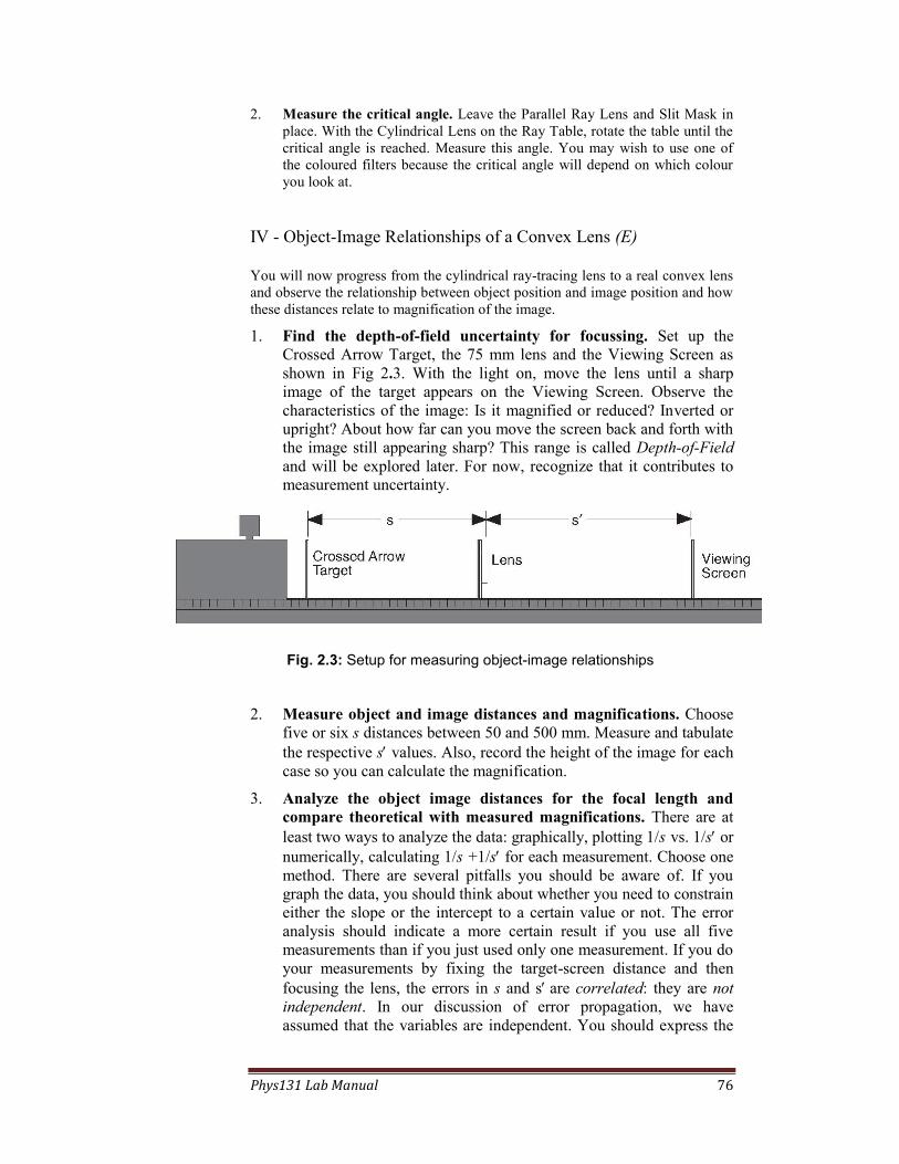
Phys131 Lab Manual 76
2. Measure the critical angle. Leave the Parallel Ray Lens and Slit Mask in
place. With the Cylindrical Lens on the Ray Table, rotate the table until the
critical angle is reached. Measure this angle. You may wish to use one of
the coloured filters because the critical angle will depend on which colour
you look at.
IV - Object-Image Relationships of a Convex Lens (E)
You will now progress from the cylindrical ray-tracing lens to a real convex lens
and observe the relationship between object position and image position and how
these distances relate to magnification of the image.
1. Find the depth-of-field uncertainty for focussing. Set up the
Crossed Arrow Target, the 75 mm lens and the Viewing Screen as
shown in Fig 2.3. With the light on, move the lens until a sharp
image of the target appears on the Viewing Screen. Observe the
characteristics of the image: Is it magnified or reduced? Inverted or
upright? About how far can you move the screen back and forth with
the image still appearing sharp? This range is called Depth-of-Field
and will be explored later. For now, recognize that it contributes to
measurement uncertainty.
Fig. 2.3: Setup for measuring object-image relationships
2. Measure object and image distances and magnifications. Choose
five or six s distances between 50 and 500 mm. Measure and tabulate
the respective s values. Also, record the height of the image for each
case so you can calculate the magnification.
3. Analyze the object image distances for the focal length and
compare theoretical with measured magnifications. There are at
least two ways to analyze the data: graphically, plotting 1/s vs. 1/s or
numerically, calculating 1/s +1/s for each measurement. Choose one
method. There are several pitfalls you should be aware of. If you
graph the data, you should think about whether you need to constrain
either the slope or the intercept to a certain value or not. The error
analysis should indicate a more certain result if you use all five
measurements than if you just used only one measurement. If you do
your measurements by fixing the target-screen distance and then
focusing the lens, the errors in s and sare correlated: they are not
independent. In our discussion of error propagation, we have
assumed that the variables are independent. You should express the

Phys131 Lab Manual 77
equation for f in terms of statistically independent variables before
applying error propagation rules.
Part V - Depth of Field and Chromatic Aberrations.
1. Find f-number and depth-of-field for the 75 mm lens. Measure the
diameter of the 75 mm lens and calculate its f-number. (f-number =
f.l./diameter.) Position the 75 mm lens to project an enlarged image of the
light bulb's filament on the screen. Record the range of viewing screen
positions within which the image appears sharp. Call this the depth-of-field.
Since this judgement is subjective, you and your partner should do it
independently.
2. Find the diameters and depths-of-field for smaller f-numbers. Common
f-stops (jargon for f-number) marked on photographic lenses are 1.4, 2, 2.8,
4, 5.6, 8, 11, 16, and 22. Small f-stops allow more light but have small
depth-of-field. Conversely, large f-stops have large depth-of-field but cut
down the light accepted. Calculate the diameters for f/8 and f/16 for a 75mm
lens. Set the Variable Aperture to give square apertures of these sizes.
(Ideally, you want a round aperture, but most camera apertures are
polygonal.) Place the aperture centred on one side of a component holder
and the lens on the other. Measure the depth-of-field at each f-stop, and note
the relative brightness of the images.
3. Observe chromatic aberration. Using a small aperture (large f-number),
place the aperture off centre and look at the image formed. Because of the
dispersion of the acrylic lens, you should see colour fringes. Note the
relative positions of the red and blue fringes and explain in terms of the lens'
dispersion. Why is the effect worse when the aperture is off centre?
Part VI - The Magnifier
When an object is between a converging lens and
its focal point, a virtual image is formed which
appears magnified and not inverted. Because the
image is virtual it cannot be projected onto a
screen; however, a viewer may see it by looking
through the lens. This is the secret of Sherlock
Holmes.
The angular magnification of a magnifier is given
by the angle subtended by the image, wherever it
may be, divided by the angle subtended by the
object at the eye's near point, xnp. Usually, xnp is
set at 25 cm, so the magnification is given by m =
xnp /f = 25/f, where f is in cm.

Phys131 Lab Manual 78
1. View magnified image through 150 mm lens. Place the viewing screen at
the 250 mm mark on the optical bench. Place the 150 mm lens between the
0 and 250 mm mark. With one of your eyes at the 0 position, look through
the lens to see a magnified image of the scale on the viewing screen. Move
the lens back and forth until you find the largest magnification that is in
focus. Where is the image? What screen-to-lens distance puts the image at
infinity?
2. Measure magnification of the lens. Try to estimate the angular
magnification by observing squared paper through the lens. Keep the paper
about 25 cm from your eye. You should see the unmagnified squares around
the lens and magnified squares through the lens. Count how many
unmagnified intervals fit in a magnified interval. Compare with xnp /f.
3. Repeat step 2 with the 75 mm lens.
VII - The Compound Microscope
The magnifier is part of a compound microscope. In the microscope the eyepiece
(or ocular) magnifies the enlarged real image projected by the objective lens at or
near the focal point of the eyepiece. Here, we use the 150 mm lens as eyepiece.
Put the crossed arrow target near the far end of the optical bench and project a
magnified image of it onto the viewing screen using the 75 mm lens. You will
probably have to illuminate the target with the light source.
The 150 mm lens, used as eyepiece, can be positioned to view the image.
After you can see the image in the viewing screen through the eyepiece, remove
the screen and turn off the light. Now you can view the magnified image directly
through both lenses. To see the best image, place your eye 10–20 cm behind the
eyepiece, not right up against it.
Try to estimate the magnification of the microscope by comparing the
magnified target scale to the scale on the viewing screen when it is placed 25 cm
from your eye. This is a little harder than for the magnifier or telescope. You
should calculate the theoretical magnification using the formulae derived from
the microscope’s geometry.
In Figure 2.5, the objective forms an inverted real image of the object as
shown. This first image is labelled the intermediate image in the diagram. It acts
as the effective object for the eyepiece lens. The eyepiece then forms a virtual
final image somewhere between infinity and the near point of the eye (25 cm).
The distance between the inside focal points of the objective and the eye-piece is
the “optical tube length” L, and it is usually standardized at 18 cm in modern
microscopes.
The overall magnification of the microscope is the product of two terms:
the magnification of the objective and the magnification of the eyepiece. We will
consider only magnitudes and not use a sign convention.
(i) The magnification of the objective is found from analysing the similar
triangles in Fig. 2.5:
mo = size of intermediate object
size of object
mo = qo–fo
fo ≈ –
L
fo .
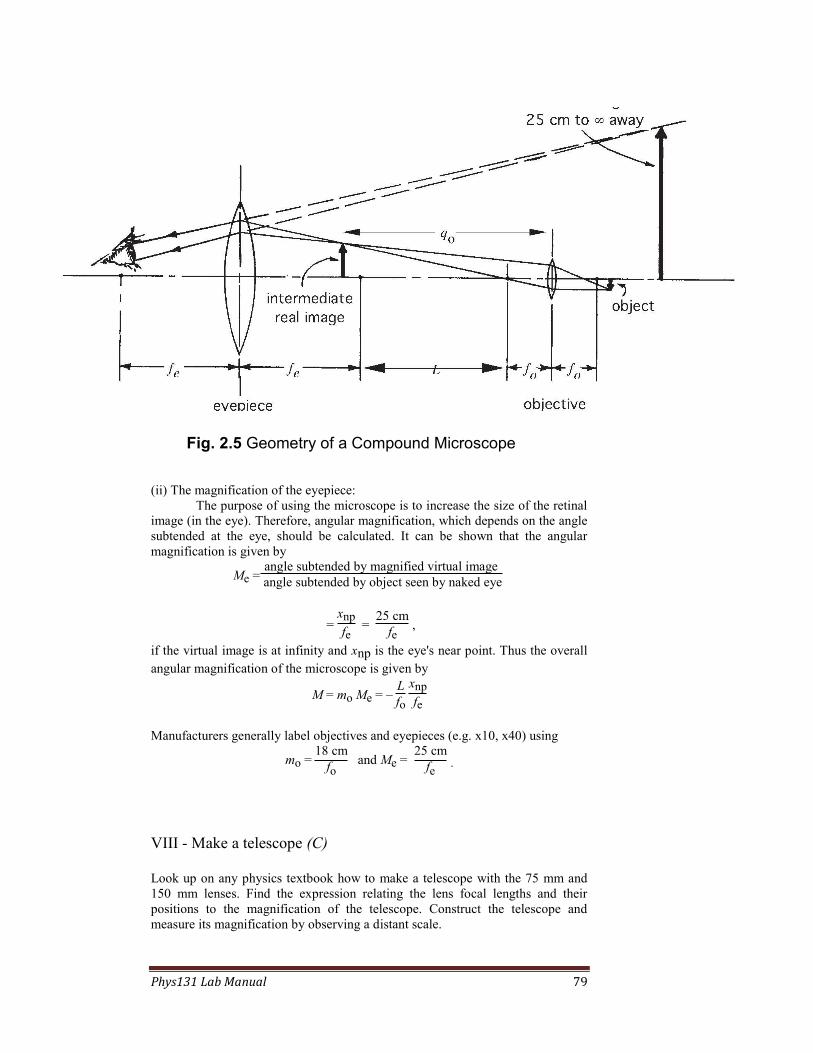
Phys131 Lab Manual 79
(ii) The magnification of the eyepiece:
The purpose of using the microscope is to increase the size of the retinal
image (in the eye). Therefore, angular magnification, which depends on the angle
subtended at the eye, should be calculated. It can be shown that the angular
magnification is given by
Me =angle subtended by magnified virtual image
angle subtended by object seen by naked eye
= xnp
fe =
25 cm
fe ,
if the virtual image is at infinity and xnp is the eye's near point. Thus the overall
angular magnification of the microscope is given by
M = mo Me = – L
fo xnp
fe
Manufacturers generally label objectives and eyepieces (e.g. x10, x40) using
mo = 18 cm
fo and Me =
25 cm
fe .
VIII - Make a telescope (C)
Look up on any physics textbook how to make a telescope with the 75 mm and
150 mm lenses. Find the expression relating the lens focal lengths and their
positions to the magnification of the telescope. Construct the telescope and
measure its magnification by observing a distant scale.
Fig. 2.5 Geometry of a Compound Microscope

Phys131 Lab Manual 80
Other things to try
•Look at the dispersion of white light produced by a prism. Find the index of
refraction as a function of the ray's angle of deviation when the rays enter and
leave the prism symmetrically (the angle of minimum deviation).
•Ask for a concave lens and convex lens to build a Galilean telescope.
•Build a reflecting telescope using a convex lens and the concave mirror.
Prelab Questions
1. The figure shows a lens focussing the image of a candle onto a white
screen. Answer the following questions
a) Is the image real or virtual?
b) If the image is larger than the object, which is greater: the source-lens
distance or the lens-image distance?
c) If the screen is removed, is it still possible to see the image from some
position? If no, explain why not. If yes, state the position and direction the
observer must look to see it.
2. The cylindrical lens of Fig. 2.2 of the lab script has a diameter of 5 cm.
What would you expect its focal length to be in the thin-lens approximation?
(Choose a reasonable index of refraction.)
3. Fig. 2.6 includes a ray diagram (using "standard" rays) for the formation of
the intermediate image by the objective lens. Complete the following ray
diagram for the eyepiece lens alone using this intermediate image as an
object and show the location of the final image.

Phys131 Lab Manual 81
Lab 7 – Polarization and Colour
.
References
Tipler (6th ed.): 31-4: Polarization.
Halliday, Resnick and Krane, (5th Ed.): Ch44: Polarization.
Objectives
I. Produce and detect linearly polarized light ( 20 min.)
II. Change polarization angle of linearly polarized light with a half-wave plate (10 min.)
III. Produce and detect circularly polarized light (20 min.)
IV. Change the handedness of circularly polarized light (15 min.)
V. Analyze circularly polarized light with a linear analyzer and vice versa (10 min.)
VI. Produce linearly polarized light by reflection at Brewster's angle (20 min.)
Take a sudden-death quiz on polarization (0–25 min.)
COLOUR
I. Observe colours produced by combining red, blue and green light. (30 min.)
II. Observe the transmitting and reflecting properties of coloured filters. (20 min.)
Apparatus
From the Optics Kit: Optical Bench, Light Source, All component holders,
Polarization Filters, Ray Table and Base, Viewing Screen, Slit Plate, Slit Mask,
Parallel Ray Lens, red, blue and green filters.
Other Stuff: Additional linear polarizer, Left circular polarizers: 2, Right circular
polarizers: 2, Quarter-wave plate, Half-wave plate
Introduction: Polarization
In this session, you will learn how to produce and detect polarized light.
The first series of short exercises will show you the properties of the filters in the
polarization kit. After you know the properties of the polarizers and retardation
plates, you will try to determine the polarization state of light coming from
various ports of the “mystery box.” Your laboratory report should list the
polarization state of the light emitted from the ports of the mystery box and
should describe the method used to reach your conclusions. There are four
different ports, and each port has one of seven possible polarization states. The
seven possibilities are
1. Unpolarized light
2. Linearly polarized light with the plane of polarization at angle to be
determined
3. Right circularly polarized light
4. Left circularly polarized light.
5. Elliptically polarized light
6. A mixture of linear and unpolarized light
7. A mixture of circular and unpolarized light
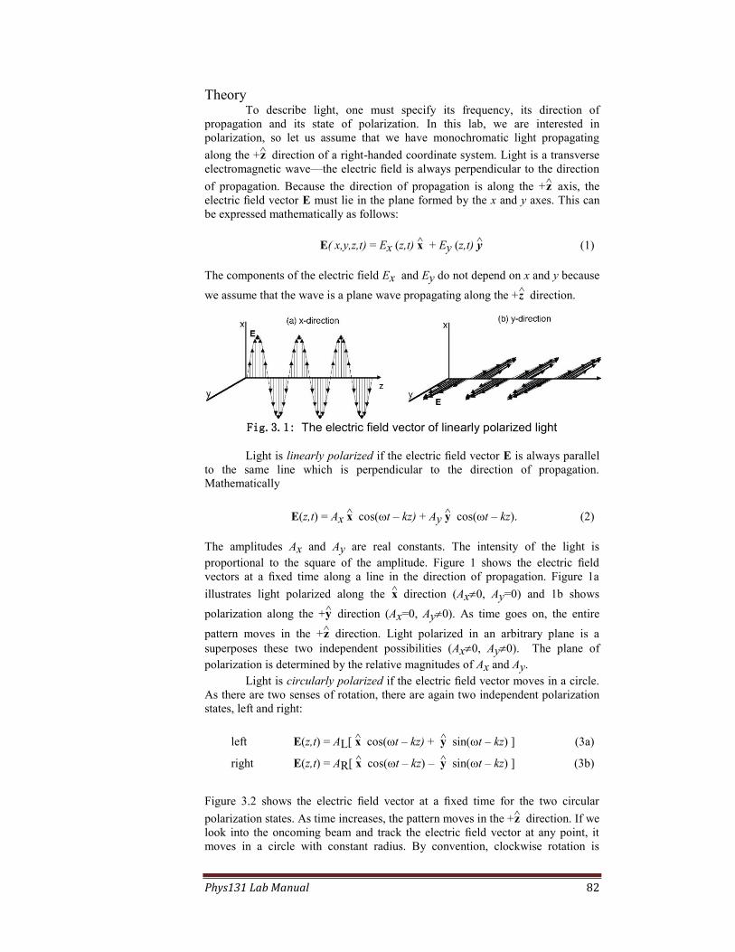
Phys131 Lab Manual 82
Theory To describe light, one must specify its frequency, its direction of
propagation and its state of polarization. In this lab, we are interested in
polarization, so let us assume that we have monochromatic light propagating
along the +z direction of a right-handed coordinate system. Light is a transverse
electromagnetic wave—the electric field is always perpendicular to the direction
of propagation. Because the direction of propagation is along the +z axis, the
electric field vector E must lie in the plane formed by the x and y axes. This can
be expressed mathematically as follows:
E( x,y,z,t) = Ex (z,t) x + Ey (z,t) y (1)
The components of the electric field Ex and Ey do not depend on x and y because
we assume that the wave is a plane wave propagating along the +z direction.
Fig.3.1: The electric field vector of linearly polarized light
Light is linearly polarized if the electric field vector E is always parallel
to the same line which is perpendicular to the direction of propagation.
Mathematically
E(z,t) = Ax x cos(t – kz) + Ay y cos(t – kz). (2)
The amplitudes Ax and Ay are real constants. The intensity of the light is
proportional to the square of the amplitude. Figure 1 shows the electric field
vectors at a fixed time along a line in the direction of propagation. Figure 1a
illustrates light polarized along the x direction (Ax0, Ay=0) and 1b shows
polarization along the +y direction (Ax=0, Ay0). As time goes on, the entire
pattern moves in the +z direction. Light polarized in an arbitrary plane is a
superposes these two independent possibilities (Ax0, Ay0). The plane of
polarization is determined by the relative magnitudes of Ax and Ay.
Light is circularly polarized if the electric field vector moves in a circle.
As there are two senses of rotation, there are again two independent polarization
states, left and right:
left E(z,t) = AL[ x cos(t – kz) + y sin(t – kz) ] (3a)
right E(z,t) = AR[ x cos(t – kz) – y sin(t – kz) ] (3b)
Figure 3.2 shows the electric field vector at a fixed time for the two circular
polarization states. As time increases, the pattern moves in the +z direction. If we
look into the oncoming beam and track the electric field vector at any point, it
moves in a circle with constant radius. By convention, clockwise rotation is

Phys131 Lab Manual 83
called right circularly polarized light because the helical path traced by the
direction of electric field at any fixed time follows the threads of a right-handed
screw.
The most general polarization state is a superposition of x and y linearly
polarized light with arbitrary amplitudes and phases. This general polarization
state can also be considered as a superposition of left and right circularly
polarized light with arbitrary amplitudes and phases of the two circular
components.
Most light sources do not produce polarized light. Individual atoms in the
source radiate independently. Although at any instant in time light received from
a radiating atom in the source has a definite state of polarization, the state of
polarization changes rapidly with time. You may think of unpolarized light as
having two polarization components (left/right or x/y) which are radiated
independently and randomly. Between polarized light which has a fixed relation
in time between the amplitude and phase of the two polarization components and
unpolarized light which has a random relation in time between the two
polarization components, is partially polarized light. Partially polarized light is a
mixture of polarized and unpolarized light.
Polarization Filters and Retardation Plates A linear polarizer produces polarized light by selectively absorbing light
polarized perpendicular to the polarization axis and transmitting light parallel to
the transmission axis. Our HN22 linear polarizers absorb more than 99.99% of
the perpendicular component and transmit 44% of the parallel component. Thus
the linear polarizer transmits 22% of incident unpolarized light. A perfect
polarizer would transmit 50% of incident unpolarized light.
Consider unpolarized light falling on a polarizer that transmits only the
components parallel to the x axis. The filtered light has amplitude A and intensity
I = A2. Let this filtered light fall on a second polarizer whose polarization axis x
is at an angle with respect to the x axis. The incident light has components A
cos and –A sin along the x and y axes. If both polarizers are perfect, the
Fig. 3.2: Left and right circular polarization

Phys131 Lab Manual 84
intensity after the second polarizer would be |A cos |2 but for the nonideal
polarizers the transmitted intensity is 0.44 |A cos |2.
You will use two retardation plates in this lab: a quarter-wave plate and
a half-wave plate. Both plates are made of a clear plastic film whose index of
refraction depends on the polarization direction of the light passing through it.
The material has two perpendicular axes called the fast axis and the slow axis. If
the light beam passing through is polarized along the material’s fast axis, the
index of refraction is nf. Likewise if the light’s axis of polarization is along the
slow axis the index of refraction is ns. The velocity of light in a material is c/n.
Light polarized along the fast axis travels faster than that polarized along the slow
axis implying nf < ns. Light polarized along an arbitrary direction can be resolved
into components parallel to the fast axis and parallel to the slow axis. Because the
faster travelling component emerges from the material first, the two polarization
components, which were in phase upon entering the film, are shifted out of phase
when they emerge. The phase shift, is given by
= 2π (ns– nf) d
where d is the thickness of the film and is the light’s wavelength.
If (ns– nf) d/ = /4, then the slower light component will emerge from
the film /4 wavelength behind the faster component. The half-wave plates are
designed so that the two polarization components are /2 wavelength out of phase
after they have passed through the film: (ns– nf) d/ = 1/2. Both the quarter- and
half-wave plates work ideally for only one wavelength in the middle of the
visible spectrum. The phase shift for other wavelengths deviates from exactly
one-quarter or exactly one-half.
Combining linear polarizers and retardation plates
Several interesting effects occur when polarizing filters are combined
with either a quarter-wave plate or a half-wave plate.
1. Linear polarizer followed by half-wave plate.
Consider a linear polarizer whose transmission axis is at an angle with
respect to the fast axis of the half-wave plate. When the light emerges from
the half-wave plate, the component polarized along the slow axis will lag
the fast component by 180° or π radians. Shifting a sine wave by 180° is the
same as inverting it (multiplying by –1). Therefore, the plane of polarization
is changed from to –. See Fig. 3.3(a).
2. Linear polarizer followed by quarter-wave plate
Let the transmission axis of the linear polarizer be ±45° with respect to the
fast axis. In this case, the slow component is shifted by 90° or π/2 radians.
Shifting a sine wave by π/2 changes it to a cosine wave. With the
polarization at 45° to the fast axis, both fast and slow components will have
the same amplitude, but the 90° phase shift will change linear polarization
to circular polarization. If is +45°, the light emerges left circularly
polarized (Fig. 3.3(b)); if is –45°, it is right circularly polarized.

Phys131 Lab Manual 85
3. Circular polarized light falls on a half-wave plate.
Circular polarization results when one polarization component lags the other
by 90°. A half wave plate will add an additional 180° lag to one component
giving a total 270° or 3π/2 radians. A 3π/2 lag (phase shift = –3π/2) appears
the same as a π/2 lead (phase shift =+π/2). Thus, right circular polarization
is transformed to left circular polarization or left to right.
Fig. 3.3(a): A half-wave plates changes the angle of linearly polarized light to its negative.
Fig. 3.3(b): Linearly polarized light passing through a quarter-wave plate at 45° becomes circularly polarized.
Fig. 3.3(c): A half-wave plate changes the handedness of circularly polarized light.
Experiment
I. Production and Detection of Linearly Polarized Light
For the following experiments, mount the light source and filters on the
optical bench as shown in figure 3.4.
A. Verify that light from the light source is unpolarized.
Look at the light source through a linear polarizer while rotating the
polarizer through 360°. If the light source is unpolarized, no variation in intensity
will be observed.
B. Verify that a linear polarizer can be used as a linear analyzer.
Produce linearly polarized light with a linear polarizer. Look at this light
through a second linear polarizer, the analyzer. When the analyzer is rotated
through 360°, alternate maxima and minima are seen every 90°. If the axis of the
first polarizer is set at an angle , then maxima are seen when the analyzer is set

Phys131 Lab Manual 86
at and +180°, and minima are seen when the analyzer is set at +90° and
+270°.
C. Understand the following non-intuitive experiment.
Mount two linear polarizers some distance apart, with their polarization
axes oriented at 90° with respect to each other. Observe that no light is
transmitted through the pair. Mount a third linear polarizer between them. Upon
rotation of the middle polarizer through 360°, maximum and minimum
transmission is observed alternately every 45°.
Fig. 3.4: Experimental setup for exploring polarization
Part II. The Half Wave Plate and Linearly Polarized Light
A. Verify that a half-wave plate has no effect on unpolarized light
Look at the light source through the half-wave plate while rotating the
half-wave plate through 360°. (The half-wave plate has its fast and slow axes
parallel to the edges.) Do you observe a variation in intensity?
B. Verify that a half-wave plate rotates the plane of polarization of linearly
polarized light.
Use a linear polarizer to produce light polarized at an angle – with
respect to the vertical. Next, mount the half-wave plate with its axes vertical and
horizontal. Look at the light passing through the linear polarizer and the half-
wave plate through a second linear polarizer. Observe minimum transmission
when the polarization axis of the second polarizer is set at +90° and +270° and
maximum transmission when its polarization axis is set at and +180°. The
half-wave plate has rotated the plane of polarization from – to +.
C. Verify that a half-wave plate has no effect on linearly polarized light when one
of its axes is parallel to the plane of polarization.
Just as in the experiment above, mount two linear polarizers some
distance apart with their polarization axes oriented at 90° with respect to one
another. Observe that no light is transmitted through the pair. Mount the half-
wave plate between the two polaroids. Observe that no light is transmitted when
the axes of the half-wave plate are parallel to the axes of the crossed linear
polarizers.
Part III. Production and Detection of Circularly Polarized Light
A. Verify that a circular polarizer run backwards acts as a circular analyzer.
Produce left circularly polarized light by allowing light from the light
source to exit the polarizer through the face marked "left circular polarizer." Look
at this light through a left and then a right circular polarizer run backwards as a
circular analyzer, i.e., through the faces marked "left circular analyzer" and "right
circular analyzer." The left circular analyzer will pass the left circularly polarized
light. The right circular analyzer will stop the left circularly polarized light.

Phys131 Lab Manual 87
Rotation of either the polarizer or the analyzer through 360° has no effect.
(Actually, you may find a small effect because the circular polarizers and
analyzers are not perfect.)
Repeat the experiment with right circularly polarized light.
B. Verify that light from the lamp is not circularly polarized.
Look at the light source through a left and a right circular analyzer.
When either analyzer is rotated through 360°, do you observe a variation in
intensity?
C. Verify that a circular polarizer passes circularly polarized light.
Produce left circularly polarized light by allowing light from the light
source to exit the polarizer through the face marked "left circular polarizer." Look
at this light through a left circular polarizer through the face marked "left circular
polarizer." Upon rotation of either polarizer through 360°, no effect is seen.
Unlike the linear polarizer, the circular polarizers have a front and a back.
The same effect should be seen when right circular polarizers are used.
D. Verify that light exiting a circular polarizer run backwards as a circular
analyzer is linearly polarized.
Look through a linear polarizer at light exiting a left or right circular
polarizer run backwards as a circular analyzer. Observe alternate maximum and
minimum transmission through the linear polarizer when the linear polarizer is
rotated through 360°. Light exiting the analyzer is linearly polarized.
E. Make a circular polarizer with the combination of a linear polarizer and a
quarter-wave plate.
Mount a linear polarizer with its polarization axis at 45°. Next, mount a
quarter-wave plate with one of its axes vertical. For your convenience, the
quarter-wave plate has been cut so that its axes are parallel to its edges. Look at
the light transmitted through the combination with a right and then by a left
circular polarizer run backwards as a circular analyzer. Light will be passed by
one and stopped by the other. The combination produces circularly polarized
light.
Rotate the quarter-wave plate by 90°, and again look at the light
transmitted through the combination through the two circular analyzers. If the left
(right) circular analyzer had passed (stopped) the light, it will now stop (pass) the
light, and if the right (left) circular analyzer has stopped (passed) the light, it will
now pass (stop) the light. Both left and right circularly polarized light can be
produced by the combination of linear polarizer and a quarter-wave plate.
Mount a linear polarizer with its polarization axis at an arbitrary angle
not 45°, say 30°, for example. Next, mount a quarter-wave plate with one of its
axes vertical. Look at the light transmitted through the combination with a right
and then a left circular polarizer run backwards as a circular analyzer. Light will
be passed by both but with different intensities. This light is elliptically polarized.
Part IV. Changing the Handedness of Circularly Polarized Light
A. Verify that the handedness of circularly polarized light changes upon
reflection by a metal surface.
Produce left (right) circular polarized light. Observe the reflected light
from a shiny metal surface at near normal incidence through a left and then
through a right circular polarizer run backwards as a circular analyzer. (It helps to
have the mirror far from the polarizer.) The right (left) circular analyzer will pass
the reflected light, and the left (right) circular analyzer will stop the light.

Phys131 Lab Manual 88
B. Understand the following non-intuitive experiment:
Place a circular polarizer on the metal mirror. Turn the polarizer over.
Look at the light reflected from the mirror through both sides of the circular
polarizer. The two experiments will have very different effects. Do for both
circular polarizers.
C. Verify that a half-wave plate changes the handedness of circularly polarized
light.
Produce left (right) circularly polarized light. Next, mount a half-wave
plate. Look at the light transmitted through a right and a left circular polarizer run
backwards as a circular analyzer. The right (left) analyzer will pass the light, and
the left (right) analyzer will stop the light. A half-wave plate changes the
handedness of circularly polarized light.
Part V. More Analysis of Polarized Light.
A. Verify that circularly polarized light is a superposition of both linear
components.
Look at circularly polarized light through a linear polarizer. Upon
rotation of the linear polarizer through 360°, why do you see very little intensity
variation?
B. Verify that linearly polarized light has both circular components.
Look at linearly polarized light through a left and a right circular
polarizer run backwards as circular analyzers. Both analyzers will pass light.
Part VI - Brewster’s Angle (E) When unpolarized light reflects from a nonmetallic surface, it is at least partially
polarized after reflection. Reflect a ray off the flat surface of the Cylindrical Lens,
and observe the reflected ray through a linear analyzer. (You may look directly at
the reflected light or project it onto a screen.) Do you observe any polarization
dependence of the reflected ray? Do the same observation on the refracted ray
emerging from the curved surface of the Cylindrical Lens.
Now polarize the incident ray by setting the linear polarizer at 90° and
placing it between the light source and the Cylindrical Lens. Project the reflected
ray onto a screen. Rotate the Ray Table and Cylindrical Lens, and observe the
intensity of the reflected ray as a function of angle. If you see a minimum or
maximum in the reflected intensity of the polarized ray, note the angle at which
this occurs. Also, record the angles of the reflected and refracted rays at this
position, and calculate the angle between them. Does this angle agree, within
experimental error,
with what you expect
from the theory of
Brewster’s angle in
your textbook?
Set the
polarizing filter at 0°
and try the same
experiment.
Try the same
experiments with the
Ray Optics Mirror.
Fig. 3.5: Setup to observe polarization of reflected light and to measure Brewster’s angle

Phys131 Lab Manual 89
COLOUR
Introduction One of the most fascinating properties of light is colour. What makes light
coloured? What is the difference between a coloured object and a black or white
one? Consider two possible theories about colour:
1. Pure light is white. When white light reflects from an object or passes through
a transparent coloured material, white light is modified to produce coloured light.
2. Pure light exists in various colours. The different colours are different species
of light. White light is obtained by mixing certain colours in right proportions.
Objects are coloured because they selectively transmit or reflect certain colours
better than others.
You may know that theory 2 is currently accepted. But if you had never
been thought about the matter, theory 1 would probably seem more reasonable.
Both descriptions agree with common experience, and even the dispersion
phenomenon you explored last time could be explained within either framework.
Here is a case where new experiments need to be devised in order to decide
between two theories. The next two exercises give you a chance to see situations
you wouldn’t ordinarily encounter. Do their results help distinguish between the
two colour theories?
Procedure
Part I - Combination of Colours
Put the Slit Plate between the light source and the Ray Table, and arrange the red
and blue-green filters so that the centre three rays are red, green and blue. Mount
the Viewing Screen on the end of the ray table and place the Parallel Ray Lens in
front of the ray table so that the three central rays converge at a point. Move the
Lens or the Viewing Screen so that the red, blue and green rays all converge
along the same line on the Viewing Screen. If you do this correctly, the
superposition of the three coloured lines will appear white. Now cover each of the
colours in sequence and observe the colour formed by the superposition of the
other two.
You can probably easily understand
what you see in terms of theory 2. Try to devise
an explanation for the colour effects you
produced using theory 1. Can you think up a
completely convincing explanation? Is it
simpler or more complex than the explanation in
terms of theory 2?
Fig. 3.6: Combining red, blue and green rays.
Red Filter
Blue/Green Filter
SlitPlate
Parallel Ray Lens
red
green
blue

Phys131 Lab Manual 90
Part II - Reflection and Transmission of Coloured Filters
Set up the Ray Table and Slit Plate so
that white rays pass over the table top.
Hold the Green Filter by hand in the
rays so that you can see both reflected
and transmitted rays.
What colour are the transmitted rays?
What colour are the reflected rays.
Place the Red Filter behind
the Green Filter so that the light passes
first through the Green Filter and then
through the Red Filter. Look into the
Green Filter. What colour are the
reflected rays now? Which rays are
reflected from the front surface of the
Green Filter, and which are reflected
from the front surface of the Red
Filter?
Place the Blue Filter over the Slit Plate so that the rays are blue. Let these
rays pass through the green filter only. What colours are reflected now? Based on
your observations, what makes the Green Filter appear green?
Other things to do
Filters are used in photography to produce special effects. If the day is clear (ha,
ha), go outside and look at the sky while turning the polarizing filters. Look at
various angles with respect to the sun, but don't look into the sun itself. Do you
know what effects the filter produces?
Red filters are used in black-and-white photography for the same purpose
that the polarizing filter is used in colour photography. Try looking through the
red filter to see its effect. What purpose could a blue filter serve in black-and-
white photography?…in colour photography?
Prelab questions
1. What is Brewster’s angle? Draw a diagram to explain how to measure
Brewster’s angle using the optics kit available in the lab.
2. Explain why it may help to wear polarizing glasses when fishing.
Fig. 3.7: Filter in the rays.

Phys131 Lab Manual 91
Lab 8 – Interference and Diffraction
References
Tipler (6th ed.): 33-3,4,8; 31-8.
Halliday, Resnick and Krane, (5th Ed.): 41-1,2,4; 42-1,2,3,5.
Objectives
I. Measure slit separation using double-slit diffraction of He-Ne laser light.
II Compare single slit diffraction patterns to double-slit patterns.
III. Construct and calibrate a portable diffraction-grating spectrometer
and use it to measure the spectra of several light sources.
IV. Observe diffraction patterns of arrays of circular apertures and a
cross.
Apparatus From the optics kit: Optical Bench, Light Source, Ray Table Base, Colour Filters,
Slit Mask, Diffraction Plate, Diffraction Grating, Diffraction Scale.
Other Stuff: He-Ne Laser, Laser Mount, Post-it Notes.
Light Sources: Na, Hg, He, H.
Introduction
I. Light Waves and Double-slit Interference (E) The preceding optics experiments could be understood using geometrical
optics. The interference and diffraction phenomena you will see in this lab cannot
be explained by ray optics and require a wave model to be understood. When
lenses, mirrors, etc. are much larger than the wavelength of light, the wave theory
gives the same results as geometrical optics. After studying interference of light,
you may come away with the impression that light is a wave and that one uses
geometrical optics only to simplify calculations where it is applicable. However,
further experiments that are beyond the level of this course show that “light =
waves” cannot be the whole story. The photoelectric effect, for example, is not
comprehensible unless we let light be composed of particles. But then how do we
explain interference?
In 1802, the supremacy of the particle theory of light was shattered by a
simple interference experiment performed by Thomas Young. He let light from a
pinhole fall on two slits in an opaque screen. If the slits were close enough to
each other, then the emerging light formed alternate bright and dark fringes on a
screen. Newton’s particle theory could not account for these bands.
A wave model proposed by Huygens proposed that each point on a wave
front be the source of a spherical wave. Thus, the superposition of all the little
spherical waves produced at a wave front add up to continue propagating the
wave forward. Placing a screen with two slits in the path of a wave will allow
only the waves passing through the slit to continue forward. Thus, two cylindrical
waves emerge from the slits that can interfere with each other at the screen. If a
line on the screen is an integer number of wavelengths from both slits, then the
interference is constructive and a bright line results. When the screen is
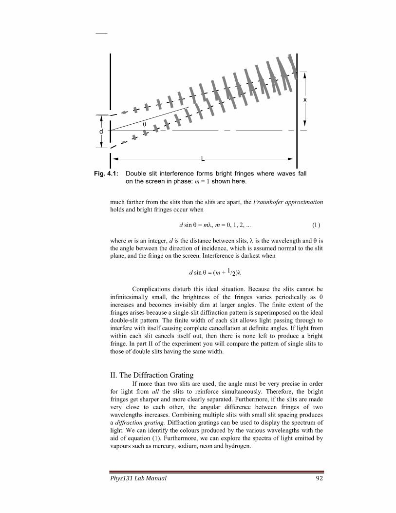
Phys131 Lab Manual 92
much farther from the slits than the slits are apart, the Fraunhofer approximation
holds and bright fringes occur when
d sin m m = 0, 1, 2, ...
where m is an integer, d is the distance between slits, is the wavelength and is
the angle between the direction of incidence, which is assumed normal to the slit
plane, and the fringe on the screen. Interference is darkest when
d sin m + 1/2)
Complications disturb this ideal situation. Because the slits cannot be
infinitesimally small, the brightness of the fringes varies periodically as
increases and becomes invisibly dim at larger angles. The finite extent of the
fringes arises because a single-slit diffraction pattern is superimposed on the ideal
double-slit pattern. The finite width of each slit allows light passing through to
interfere with itself causing complete cancellation at definite angles. If light from
within each slit cancels itself out, then there is none left to produce a bright
fringe. In part II of the experiment you will compare the pattern of single slits to
those of double slits having the same width.
II. The Diffraction Grating If more than two slits are used, the angle must be very precise in order
for light from all the slits to reinforce simultaneously. Therefore, the bright
fringes get sharper and more clearly separated. Furthermore, if the slits are made
very close to each other, the angular difference between fringes of two
wavelengths increases. Combining multiple slits with small slit spacing produces
a diffraction grating. Diffraction gratings can be used to display the spectrum of
light. We can identify the colours produced by the various wavelengths with the
aid of equation (1). Furthermore, we can explore the spectra of light emitted by
vapours such as mercury, sodium, neon and hydrogen.
Fig. 4.1: Double slit interference forms bright fringes where waves fall
on the screen in phase: m = 1 shown here.
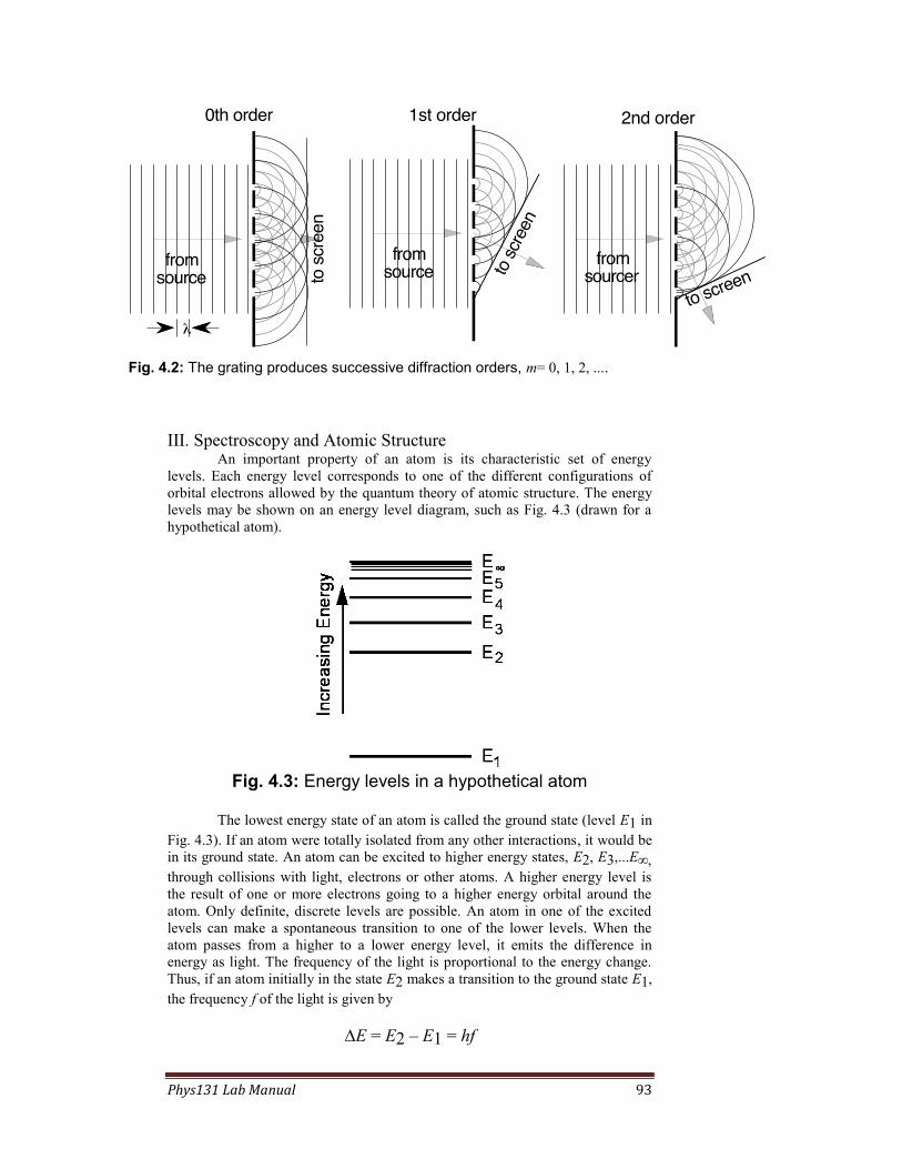
Phys131 Lab Manual 93
III. Spectroscopy and Atomic Structure An important property of an atom is its characteristic set of energy
levels. Each energy level corresponds to one of the different configurations of
orbital electrons allowed by the quantum theory of atomic structure. The energy
levels may be shown on an energy level diagram, such as Fig. 4.3 (drawn for a
hypothetical atom).
Fig. 4.3: Energy levels in a hypothetical atom
The lowest energy state of an atom is called the ground state (level E1 in
Fig. 4.3). If an atom were totally isolated from any other interactions, it would be
in its ground state. An atom can be excited to higher energy states, E2, E3,...E
through collisions with light, electrons or other atoms. A higher energy level is
the result of one or more electrons going to a higher energy orbital around the
atom. Only definite, discrete levels are possible. An atom in one of the excited
levels can make a spontaneous transition to one of the lower levels. When the
atom passes from a higher to a lower energy level, it emits the difference in
energy as light. The frequency of the light is proportional to the energy change.
Thus, if an atom initially in the state E2 makes a transition to the ground state E1,
the frequency f of the light is given by
E = E2 – E1 = hf
Fig. 4.2: The grating produces successive diffraction orders, m= 0, 1, 2, ....

Phys131 Lab Manual 94
where h is a universal constant called Planck's constant. The observation that only
certain frequencies of light are emitted by atoms agrees with the existence of
discrete energy levels available to the excited atom.
In optical spectroscopy, we do not measure the frequency f directly but
rather the wavelength . For any wave motion, the frequency and the wavelength
are related through
f = c
,
where c is the velocity of the wave in the medium. Since we are dealing with
wavelengths in air, c is to be interpreted as the velocity of light in air for this
experiment. The energy difference E can now be expressed in terms of the
wavelength through
E = hc
.
In optics, it is customary to measure the wavelength in nanometers
(10-9 m = 1 nanometer) and the energy difference in electron-volts (1 eV = the
energy gained by an electron accelerated through a potential difference of 1 volt.)
The relationship between the energy difference and the wavelength can be written
as
E = 1239.8
(in nm) eV
The set of energy levels is characteristic of the atomic species, so that
each atom emits its own characteristic spectrum. The hydrogen atom with only
one electron has a very simple energy level structure. The energy levels are given
by
En = –13.6 eV
n2 , n = 1, 2, ...,
The integer n is called the quantum number of the energy level. For a low-
pressure discharge, the energy levels are sharp, and the transitions from higher
energy levels to lower ones produce a line spectrum. The line spectrum of the
hydrogen atom is given by the Rydberg-Ritz formula:
2
1
2
2
1 11967810
1
nnm.
,
where n1 and n2 are the quantum numbers of the two energy levels. The visible
(Balmer series) spectrum was the first to be observed and corresponds to n2 = 2.
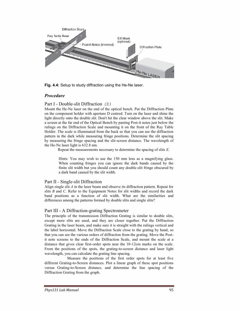
Phys131 Lab Manual 95
Fig. 4.4: Setup to study diffraction using the He-Ne laser.
Procedure
Part I - Double-slit Diffraction (E) Mount the He-Ne laser on the end of the optical bench. Put the Diffraction Plate
on the component holder with aperture D centred. Turn on the laser and shine the
light directly onto the double slit. Don't hit the clear window above the slit. Make
a screen at the far end of the Optical Bench by pasting Post-it notes just below the
rulings on the Diffraction Scale and mounting it on the front of the Ray Table
Holder. The scale is illuminated from the back so that you can see the diffraction
pattern in the dark while measuring fringe positions. Determine the slit spacing
by measuring the fringe spacing and the slit-screen distance. The wavelength of
the He-Ne laser light is 632.8 nm.
Repeat the measurements necessary to determine the spacing of slits E.
Hints: You may wish to use the 150 mm lens as a magnifying glass.
When counting fringes you can ignore the dark bands caused by the
finite slit width but you should count any double-slit fringe obscured by
a dark band caused by the slit width.
Part II - Single-slit Diffraction Align single slit A in the laser beam and observe its diffraction pattern. Repeat for
slits B and C. Refer to the Equipment Notes for slit widths and record the dark
band positions as a function of slit width. What are the similarities and
differences among the patterns formed by double slits and single slits?
Part III - A Diffraction-grating Spectrometer The principle of the transmission Diffraction Grating is similar to double slits,
except more slits are used, and they are closer together. Put the Diffraction
Grating in the laser beam, and make sure it is straight with the rulings vertical and
the label horizontal. Move the Diffraction Scale close to the grating by hand, so
that you can see the various orders of diffraction from the grating. Move the Post-
it note screens to the ends of the Diffraction Scale, and mount the scale at a
distance that gives clear first-order spots near the 10-12cm marks on the scale.
From the positions of the spots, the grating-to-screen distance and laser light
wavelength, you can calculate the grating line spacing.
Measure the positions of the first order spots for at least five
different Grating-to-Screen distances. Plot a linear graph of these spot positions
versus Grating-to-Screen distance, and determine the line spacing of the
Diffraction Grating from the graph.

Phys131 Lab Manual 96
Make a scale for your spectrometer by calculating the positions where
the following wavelengths of light should fall on the Diffraction Scale: 400 nm,
450 nm, 500 nm, 550 nm, 600 nm, 650 nm, 700 nm. Mark the wavelength scale
on the Post-it notes in dark black. Then check your calibration by shining the
laser beam's first order spot on your homemade scale. If the spot does not fall
near 630 nm, adjust the Diffraction Scale-to-Grating distance until it is correct.
Fig. 4.6: Geometry of the diffraction-grating spectrometer
Fig. 4.5: A diffraction-grating spectrometer
DIFFRACTION GRA
TING
Diffraction Grating
Slit Mask
Incandescent Light Source(Do not use Laser!)

Phys131 Lab Manual 97
Turn off the Laser, unplug it and remove it from the optical bench.
Put the Incandescent Light Source at the other end of the optical bench
so that it shines through the slit in the Diffraction Scale. Centre the Slit Mask
over the Diffraction Grating on the other side of its component holder. Turn on
the Incandescent Light Source, and view its spectrum by looking through the
Diffraction Grating towards the scale you made. This geometry is different from
that for used to project the pattern with a laser, but the angles you see are the
same. You should see a rainbow of colours, from which you can estimate the
wavelengths of the spectral colours from blue to red. Put a coloured filter over the
light source and look at the spectral range of each filter. You can place the
blue/green filter so that you can see both spectra, one on top of the other.
The following light sources should be available in the lab: hydrogen,
mercury, helium and sodium. Observe the spectral lines of their light. These
spectra are caused by electron transitions between atomic energy levels in the
atoms. Hydrogen has only one electron per atom and therefore has the simplest
atomic structure and spectrum. You should be able to see three lines of the
hydrogen spectrum, red, blue and violet. Measure their wavelengths and see
whether they agree with the Rydberg-Ritz formula with n2 =2. Find the values of
n1 that give the lines you have observed. Calculate the energies of the energy
levels between which the electron jumps to produce the observed lines.

Phys131 Lab Manual 98
Equipment Note: The Laser Mount
Instructions on using the laser mount will be provided in the lab.
The Diffraction Plate
The Diffraction Plate has ten different apertures labelled A through F.
Above each line of five apertures there is a clear window, which is not a
part of the aperture. This window allows you to look through the plate and
see a pattern formed by the aperture as well as read the Diffraction Scale
through the window. You will not need to use this window with the laser
experiments. Table I lists the Diffraction Plate apertures.
Fig. 4.7: Diffraction Plate
Table I: Diffraction Plate Apertures
Pattern
No. Slits
Slit Width
(mm)
Slit Spacing Centre-to-centre
(mm)
A 1 0.04 B 1 0.08 C 1 0.16 D 2 0.04 0.125 E 2 0.04 0.250 F 2 0.08 0.250 G 10 0.06 0.250 H 2 (crossed) 0.04 I 225 Random Circular Apertures (0.06 mm dia.) J 15x15 Array of Circular Apertures (0.06 mm
dia.)
. . . . . . . .. . . . . .. . .. . . . .. . . . .. . . . . . . .. . . . . .. . .. . . . .. . . . .
. . . . . . . .. . . . . .. . .. . . . .. . . . .. . . . . . . .. . . . . .. . .. . . . .. . . . .
. . . . . . . .. . . . . .. . .. . . . .. . . . ...............................................................................................................................
.....................
.....................
.....................
.....................
.....................
.....................
DIFFRACTION PLATEA B C D E
DIFFRACTION PLATEJ I H G F

Phys131 Lab Manual 99
Prelab Questions
1. The He-Ne laser shines through a slit in the diffraction plate that is 50 cm from
the screen. What fringe spacing would you expect for slits E and F if the stated
slit spacing is correct? What difference should there be between the patterns
produced by slits D and E? (See Equipment Note on the previous page.)
2. In Part III, you use the diffraction grating to make a simple spectrometer.
Assume the grating is 60 cm from the diffraction scale and has a line spacing of
5276 lines/cm. Calculate where on the diffraction scale the visible lines of the
Balmer Series of the Hydrogen atom's spectrum should appear. Make a table
showing wavelengths and line positions for n2 = 2, n
1 = 3, 4, and 5. Of what
significance are the wavelengths you calculate when n1 = 1? How about n
1 = 2
when n2 = 2?

Phys131 Lab Manual 100
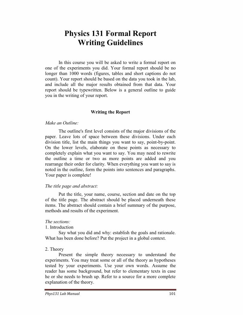
Phys131 Lab Manual 101
Physics 131 Formal Report
Writing Guidelines
In this course you will be asked to write a formal report on
one of the experiments you did. Your formal report should be no
longer than 1000 words (figures, tables and short captions do not
count). Your report should be based on the data you took in the lab,
and include all the major results obtained from that data. Your
report should be typewritten. Below is a general outline to guide
you in the writing of your report.
Writing the Report
Make an Outline:
The outline's first level consists of the major divisions of the
paper. Leave lots of space between these divisions. Under each
division title, list the main things you want to say, point-by-point.
On the lower levels, elaborate on these points as necessary to
completely explain what you want to say. You may need to rewrite
the outline a time or two as more points are added and you
rearrange their order for clarity. When everything you want to say is
noted in the outline, form the points into sentences and paragraphs.
Your paper is complete!
The title page and abstract:
Put the title, your name, course, section and date on the top
of the title page. The abstract should be placed underneath these
items. The abstract should contain a brief summary of the purpose,
methods and results of the experiment.
The sections:
1. Introduction
Say what you did and why: establish the goals and rationale.
What has been done before? Put the project in a global context.
2. Theory
Present the simple theory necessary to understand the
experiments. You may treat some or all of the theory as hypotheses
tested by your experiments. Use your own words. Assume the
reader has some background, but refer to elementary texts in case
he or she needs to brush up. Refer to a source for a more complete
explanation of the theory.

Phys131 Lab Manual 102
3. Experiment
Clearly describe what you did. Do not over-use the passive.
Clear and simple diagrams showing essential features of the
apparatus are necessary.
4. Results
Show your results in graphical form, if possible. A complete
table of the raw data is usually not necessary. If calculated
quantities are presented, refer to the relevant equation in the theory
section, but don't show the detailed steps in the calculation.
Uncertainties on both the raw data and calculated quantities should
be indicated, but don't show detailed error calculations or
methods—these should be known by the reader.
5. Discussion or Conclusions (Could be combined with Results)
Indicate how nearly you achieved the goals mentioned in the
introduction. Discuss the meaning of the results in terms of the
theory presented. Do experimental results and theory agree within
experimental error? If not, suggest why not, and propose what
further experiments may be needed. Make sure that your
conclusions follow from your experimental results, Treat your own
data and results objectively, and don't try slant the discussion to
agree with your preconceived notions when the data do not
support them.
Equations:
Very simple equations may be written in-line. Complex
equations with lots of subscripts, superscripts, compound fractions,
integrals, or summations look clumsy in-line and should be
displayed centred with a blank line above and below. Any equation
that is referred to elsewhere in the text should be displayed and
numbered at the right margin. Always define every symbol in all
equations.
Figures:
Figures should usually have a short caption beneath them. A
caption makes it easier to understand for someone browsing through
the pages. If there is more than one figure, the
captions should start with a figure number. The text of the paper
should refer to every figure.
Points on style:
1. Use the active voice.

Phys131 Lab Manual 103
Passive
Control of the furnace is provided by a
thermostat.
Dolphins were taught by researchers in
Hawaii to learn new behaviour
Active
A thermostat controls the furnace.
Researchers in Hawaii taught
dolphins to learn new behaviour.
Use the passive when the doer the action is unknown or unimportant.
2. Use simple rather than complex language.
Complex
Another very important consequence of
Einstein's theory of relativity that does
not follow from classical mechanics is
the prediction that even when a body
having mass is at rest, and hence has no
kinetic energy, there still remains a
fixed and constant quantity of energy
within this body.
Simple
According to the theory of special relativity,
even a body at rest contains energy.
3. Delete words, sentences, and phrases that do not add to your meaning.
Wordy
It is most useful to keep in mind that the
term diabetes mellitus refers to a whole
spectrum of disorders.
In the majority of cases, the data
provided by direct examination of fresh
material under the lens of the
microscope are insufficient for the
proper identification of bacteria.
Concise
Diabetes mellitus refers to a whole spectrum
of disorders.
Often, bacteria cannot be identified under
the
microscope.
4. Use specific, concrete terms rather than vague generalities.
Vague
Our new scrubber means big savings for
Samson Power.
The sun is hot.
Specific
Aircom's scrubbing system saves Samson
$7,000 every day.
The sun is hot—almost 10,000°F at its
surface.

Phys131 Lab Manual 104
The expedition was delayed for a time
because of unfavourable conditions.
The expedition was delayed one week
because of snowstorms.
5. Use the past tense to describe your experimental work and
results.
6. In most other writings, use the present tense.
Hypotheses, principles, theories, facts and other general
truths are expressed in the present tense.
7. Avoid needlessly technical language.
Too technical
The moon was in syzygy.
Maximize the decible level.
.
Clearer
The moon was aligned with the
sun and the earth
Turn up the sound.
8. Keep ideas in writing parallel.
Not parallel
The tube runs into the chest cavity, across
the lungs and plunges down into the
stomach.
.
Parallel
The tube runs into the chest
cavity, across the lungs and
down into the stomach.
References:
Robert W. Bly and Gary Blake, Technical Writing, (McGraw Hill, New
York) 1982. Library call
no. T11 B63.
William Strunk Jr. and E.B. White, The Elements of Style, 3rd ed.,
(Macmillan, New York) 1979
Library call no. PE1408 S772 1979 (Reference)
The Elements of Style, 1st ed. is available on the world wide web at
http://www.columbia.edu/acis/bartleby/strunk

Phys131 Lab Manual 105
Editing your writing
The following shows how to edit your text to for conciseness and
clarity. The “original abstract” is typical for a first draft and is taken
from a student’s report in a previous semester. Comparing the
original with the edited version should help you to learn how to edit
your own writing.
Original Abstract
First, I made qualitative observations investigating the nature
of images produced by concave lenses and convex lenses of various
focal lengths. I found that convex lenses with small
focal lengths magnified a printed page the most. The object
appeared smaller through the concave lens. Distant objects observed
through both concave and convex lenses are smaller but are
inverted when observed through the convex lens. These
observations agree with the ray approximation methods (see figures
two to four) of studying geometric optics as presented by Serway
[1].
Three different methods were used to determine the focal
length of various lenses: the image of a distant object method;
object image methods; and the autocollimation method. Using these
methods, I determined the focal length of two convex lenses to
within various degrees of the rated value of the lens. The
autocollimation method was the most accurate with a percentage
difference of 1.3% from the rated value. Object image methods
were within 2.6% of the rated
focal length. The first method was the least accurate with a
percentage difference of 7.0%. These uncertainties are due to
systematic errors in the method and different amounts of random
error.
Finally, a basic microscope was constructed and its
magnification measured. The magnification was approximately 100
times. Due to the very large degree of uncertainty in the apparatus,
we were interested chiefly in the order of magnitude of this value.
The calculated magnification was 66.
Revised Abstract
In this paper, I discuss qualitative observations of images
through lenses, compare three methods of measuring focal lengths
and describe a compound microscope made from thin lenses.
Objects always appear upright, but smaller, when observed
through a concave lens. When one observes an object through a
convex lens, the image is magnified and upright if the lens–object
distance is less than the focal length—the magnification being

Phys131 Lab Manual 106
larger for shorter focal-lengthlenses. If the convex-lens-to-object
distance is greater than the focal-length, the virtual image is smaller
and inverted. These observations agree with the ray model of
geometric optics.
I measured the focal lengths of two calibrated convex lenses
using three methods: the distant-object image method; the near-
object image method; and the autocollimation method. The
deviations of the measurements from the nominal values were 7%,
2.6%, and 1.3% respectively for the three methods. The origins of
the systematic and random errors in the three methods are
discussed.
Finally, I designed a compound microscope to have an
angular magnification of 66. When built, the magnification was
approximately 100.

Phys131 Lab Manual 107
A Few Basic DOs and DON'Ts
DO
Do use relatively large font and generous
line spacing, e.g., 12 pt Times and 18 pt
line spacing or typewriter elite (10 pt
Courier) and 1.5 or double space.
Do put your name, section, student number
and all of the abstract on the title page.
Do staple your paper in the upper left-hand
corner.
Do use your own words to describe the
experiment.
Do use the affirmative: "We adjusted the
string's length to 1 m."
Do make your own simple but complete
line drawings of the apparatus with labels
of parts. Identify mathematical variables
on the drawings if possible.
Do prepare neat publication-quality graphs
of data which fit in with the text and are
easily legible.
DON'T
Don't use very small typeface with
cramped line spacing., e.g., 10 pt Times
and 11 pt line spacing. (There is no
room to write comments.)
Don't omit your name, start the
introduction on the title page, or put all
of or a part of the abstract inside.
Don't put the report in a presentation
cover or folder. Don't just crimp the
corner and hope the pages will not fall
apart.
Don't copy large sections of the lab
manual or other book.
Don't use the imperative: "Adjust the
string's length to 1 m."
Don't scan in or photocopy fancy
pictures from the lab manual or other
books.
Don't tear out or photocopy graphs from
you lab book and stick them in your
formal
report.

Phys131 Lab Manual 108