Physics 116CGeiger Counter, Statistics, and Radioactive Decay

Rev. 4/12/2007

The goals of this two-week lab are

1. to investigate the Geiger counter and basic data acquisition techniques with LabVIEW,

2. to investigate counting statistics (Poisson and Gaussian distributions as limits of the binomialdistribution),

3. to collect data and perform a least-squares fit to measure the mean life of unstable 116Innuclei and estimate the error in the mean life,

4. to evaluate the goodness of fit using the χ2 distribution, and

5. to make a complete report on your experiment.

Begin by reading the information from the Physics 122 Lab manual on Geiger counter basics and116In radioactive decay. It is provided at the end of this writeup. We have modified the 122 Labprocedure to use a National Instruments E-Series PCI data acquisition (DAQ) card and a LabVIEWprogram to do the counting and timing more accurately and faster than could have been done byhand. The program can also display the major results rapidly. Also, we will investigate the Geigercounter pulses in more detail.

Precautions with Geiger tube:

• Leave the cable from the Geiger counter controller to the Geiger tube in place at all times.The connector on the controller can carry a voltage of order 1000 V. If you leave the cablefrom the tube connected, nothing else can get connected to it by mistake (including fingers!).

• Leave the Geiger tube in its holder. It has a thin front window which could be broken.

Overview

The block diagram of the circuit is shown in Fig. 1. The idea is to use a continuously runningcounter which can be read at regular intervals by the computer to take the data (number of countsper interval). The computer program can make histograms to be read out manually and comparedwith statistical theory and saved to a file for further analysis. The timing accuracy is at least ofthe order of a few ms, which is sufficient for this application. (Greater timing accuracy could beachieved with external gating pulses.)

1

This experiment exemplifies a nuclear or particle physics experiment at possibly the simplest level.Particles (e.g., β−, otherwise known as energetic electrons) enter on the left, proceed throughdetectors and produce electronic pulses. These go through pulse shapers, data acquisition circuitsand a computer, producing data files and histograms, which come out at the right. These result inpublications, or at least in lab reports.

Figure 1: Circuit block diagram.

The salient features of the Geiger counter controller are shown in Fig. 2. It has a pair of terminalson the back marked “Oscilloscope” (bottom one is ground). The output is a fast-rising pulse withheight of approx. 2.5 V and a decay time constant≈ 200 µs superimposed on a DC pedestal≈ 5 V.

Figure 2: Geiger counter control box.

To get a logic pulse for the computer interface, we need to build a circuit to trigger on pulsesexceeding a certain amplitude above the pedestal. That is the circuit in Fig. 3.

The data acquisition VI was adapted from an example called Count Edges (DAQ-STC).vi includedin the daq-stc.llb library file which came with the Student Edition of LabVIEW. The original pro-gram counted leading edges of pulses from the DAQ counter. It was modified to make a fixednumber of count samples, store them in an array and make a histogram of the results. The VIcontrol panel is shown in Fig. 4 and the VI block diagram in Fig. 5.

2

Figure 3: AC-coupled Schmitt trigger circuit for Geiger counter.

Procedure for First Week

1. Record your observations and make preliminary curves in a loose leaf notebook (preferablyquadrille-ruled engineering paper). Save files you have developed (data or VIs) in your diskspace on “MyUCDavis” (you can upload and download files using a web browser) or on aUSB flash drive.

The lab will be continued the following week to make a useful physical measurement withstated uncertainties (116In excited state mean life). A full lab report will be required at theend covering both weeks.

2. Check and turn on Geiger counter

Remember the warning above not to disturb the connection to the Geiger counter itself, butverify that it is connected to the control box HV. Turn on the Geiger counter control box, setthe HV knob fully CCW (low voltage) and turn on the Geiger counter HV. We turn on thisequipment at this point to let its temperature stabilize.

3. Trigger circuit

Wire the trigger circuit shown in Fig. 3. Use the lower left corner of the prototype boardarray. Be reasonably neat and use 5 V and ground busses appropriately. The input shouldbe from the BNC connector on the left and the output to the BNC connector on the right.Connect the output to the DAQ interface panel BNC connector marked PFI0/TRIG1.

4. LabVIEW VI

Load the DAQ program (called geiger all v2.vi). In the lab, become familiar with the dia-gram, particularly that within and to the right of the For loop. (The block diagram shown inthis report is an earlier version without file output but the basic structure is the same). TheDAQ counter I/O is from the example; understanding details of the DAQ sub-vi’s will bedeferred until later.

Note how the loop delay timer waits until a fixed multiple of a system clock (in ms) beforereading the continuously running counter and exiting the loop. The Geiger count sample forthe current interval is found by subtracting the counter reading from the previous iteration.This is put in an array (Count Array). But first the zeroth and first element are deleted: thezeroth element winds up being the initial value of the counter (0) and the first element the

3

Figure 4: Geiger counter statistics front panel (DAQ setup not shown).

value from the incomplete period of the first loop iteration (the loop is only synchronizedafter the first loop ends).

Also observe how the histogram works. You specify the minimum and maximum limits ofthe histogram and the number of bins. For example, if you wanted to have bins correspondingto 990 to 1010 with 20 bins, you would enter these numbers. The histogram x-axis wouldthen show 0 to 20. The lower bin edge of the lowest bin would correspond to 990, the upperedge of highest bin would correspond to 1010 and each bin width would correspond to 1count. The “inclusion” parameter has been set to “lower” so a number on the lower binboundary is assigned to that bin. There is a quirk, though, in that the histogram maximumvalue is assigned to the highest bin. This would normally be the lower boundary of the nexthigher bin so if there were one, this value should go there, but in this case, it is counted in thehighest bin. For example, if you had entered the 21 data values, 990 through 1010, each binwould contain one count except for the highest bin, which would contain two entries, one for“1009” (corresponding to the lower bin edge) and another one for “1010” (corresponding tothe histogram maximum). This will not be important if you set up your histograms so theminimum and maximum bins are not populated. In any case, you should be aware of this

4

Figure 5: Geiger counter statistics VI block diagram (earlier version without file I/O).

behavior of the histogram VI.

The histogram display shows the bin contents with bin number along the bottom. (This couldbe improved by using an xy plot for the histogram display and using the x-axis informationfrom the histogram VI to enter the proper x axis values.)

The samples outside the histogram range are also tallied to the lower left of the display,above the output arrays. Running tallies during program execution are at the upper right.The histogram is not produced until the end of the run.

The time stamp array represents the time in s since Friday, January 1, 2004 Universal Time.This is here mainly for the radioactive decay measurement.

5. Test the count accuracy and repeatability

Use the signal generator to produce a 1 kHz square wave of 2 V amplitude (4 v peak-to-peak)and connect it to the input of your trigger circuit on the breadboard.

Now set your VI to count 10 samples of 1000 ms. As they come in, watch the count in-crement (it should be close to 1000 but with variations). You can review them when youare done and set the histogram accordingly for a longer run. The bin settings I gave in thesection above would be appropriate. With a longer run (50 samples, say) you can accumulatestatistics on the counting accuracy.

Record the histogram, measured frequency and signal generator frequency.

When you are finished, disconnect the signal generator from your trigger circuit input andconnect the cable from the Geiger counter Control Box output instead. The cable connects tothe scope output screw terminals on the back of the control box (bottom terminal is ground).

5

6. Set Geiger counter operating voltage

The 137Cs source should be in the second slot from the top of the Geiger tube holder. (Cau-tion: don’t touch the source. Leave it in its tray at all times. The TA or lab assistant willprovide the sources and deal with moving them from place to place.) Be sure the Geigercounter control box is set to count. We will leave it in this mode at all times. Also, don’tpush the reset button. It can generate spurious pulses in the output to the discriminator. Thissource emits energetic β− particles which enter the Geiger tube through the thin window andionize the gas to cause output pulses.

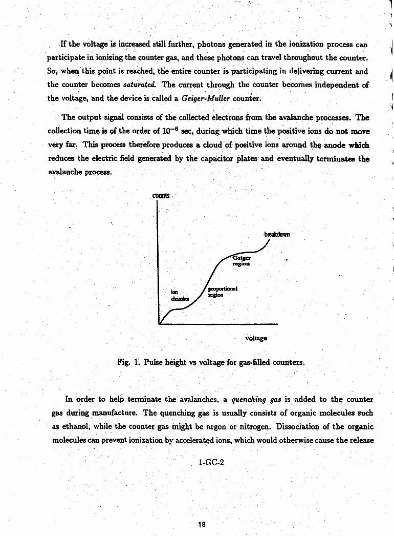
(a) Finding the thresholdUse the LabVIEW VI (not the counter control box itself–leave it counting continuously;it will have a somewhat lower counting threshold).Be careful not to exceed 1000 V. If you hear a ticking sound from the counter (HVbreakdown), reduce the voltage immediately and call the TA.Set the VI to count a large number of samples (10000, say) with a short count interval(100 ms). Start the VI and watch the count increment window as you slowly increasethe Geiger counter HV from its minimum setting. If the VI terminates, start it again.Find the minimum HV setting for which you get reliable counting. Record this thresh-old voltage.

(b) Making a plateau curveStart at the next 50 V HV multiple above the threshold (e.g., if the threshold was 730 V,start at 750). Set the VI to acquire 1 sample with a 10000 ms count interval and startthe program. After 20 s or so, you will get a count measurement (0th element of thecount array). Record this and the voltage. Now increase the voltage in 50 V incrementsup to 1000 V (or 300 V above threshold, whichever is less–don’t exceed 1000 V) andrepeat the count measurements. You should get samples, ni, of order 1000 counts eachon the plateau.Make a (hand-drawn) graph of your result with error bars. We assume Poisson statisticshere, so we can estimate σi =

√ni. The threshold voltage in our discriminator is too

high to observe the linear or proportional region of the counter, but there should bea gently rising linear plateau in the Geiger region above the threshold and to the leftof any sharp rise at large voltages. Set the voltage near the center of this plateau andrecord this operating voltage (it will probably be ≈ 100 V above your first measuredpoint above the counting threshold).Fig. 6 shows a typical plateau curve and the chosen operating point.

6

Figure 6: Geiger counter plateau curve.

7. Observe Geiger pulses and dead time

Sketch the pulses at four points: trigger circuit input, comparator “-” input, comparatoroutput and trigger circuit output. Note: check the output pulse at a high sweep speed to besure there are no spurious extra pulses at the end (glitches) which could be counted by the20 MHz counter. (The low pass filter at the output is provided to suppress such glitches.)

Now set the oscilloscope time base to 50 µs/division. The source should now be in thetop slot, nearest the tube. You should see additional output pulses on the same trace as thetriggering pulses. These appear at random, following a uniform distribution except near thebeginning of the trace. Estimate how long this gap lasts where no additional pulses are seen.This is the overall dead time of the circuit. Record this information.

Actually, the counter is recovering from delivering its previous pulse toward the end of thisperiod. If you hook the scope probe to the comparator “-” input, you should see small pulsesoccasionally near the end of the deadtime region below the 0.5 V threshold (scope triggerlevel needs to be set low enough to capture them). These pulses increase in size until theyreach the maximum. This is the Geiger counter “recovery” region. See if you can observethis.

8. VI file output

An output text file of the samples is written so other histogram binning could be done ifdesired using LabVIEW or other analysis software. We also need this capability for theradioactive decay experiment. Examine how this works and check that the data agree withwhat you expect. The text entry field on the VI front panel provides a place where you cantype identification information for the run before you start the VI. This information is outputas the first line in the output file.

7

9. Observe Poisson statistics with mean near 0

This should be done with the source in the bottom slot (away from the tube) and with arelatively short count interval (100 ms, say). The mean number of counts should be of order2 or 3; be sure it is low enough that you get a reasonable number of zero count samples. Thehistogram should be set to have bin widths of one count and start at 0.

Do a run of 10 samples and check that the histogram of the samples ni is correct–i.e., makethe histogram by hand and see that it agrees with the computer. Include the check histogramin your lab notes (this is to verify that the software is working as expected). As this is done(or redo if necessary), check that the count increments on the Geiger counter scale roughlyagree with what you see with the program. Don’t reset the Geiger counter readout–thiscauses spurious pulses to be injected into the discriminator. Just read the counter on the flyand subtract, as the program is doing. At this low rate, you should be able to check thatthe two tallies agree closely. If not, discuss with the instructor. Note: lesson learned fromexperience!

Do a 100 sample run under these conditions and record the histogram contents in your data.Be sure to record the conditions of the run, particularly the histogram setup. Be sure yourupper limit is such that there are no overflows. Be sure the histogram looks reasonable beforeproceeding.

10. Observe Poisson statistics with mean > 100 and compare with normal distribution

The source should now be in the slot second from the top. A counting interval of 5000 mswill probably be appropriate for this section. Make a histogram with 5 counts per bin whichincludes the entire distribution on ni (within at least 2σ) and has boundaries that are easyto understand. For example, if the expected number of counts were 400, you could make ahistogram with lower limit 350, upper limit 450 and 20 bins.

Do a run of 100 samples, save the output data file for further analysis and record the his-togram in your lab notes. Be sure to record the histogram limits. Make sure the histogramlooks reasonable.

11. Suggested analysis and writeup for this part

The idea is to plot the histograms and compare with Poisson (low rate) or Gaussian (highrate) statistics. For the high rate data, we want to compare with the Gaussian limit by calcu-lating the number of counts expected in each bin using differences of the Gaussian cumula-tive distribution function, given the measured mean value.

The writeup should be brief but complete. It should briefly describe your procedure and theequipment used, including Geiger counter operation.

8

Outline of Procedure for Second Week

1. Prepare equipment and program

For this week’s lab, the first hour will be spent completing unfinished work from last week,becoming familiar with the complete program for data acquisition (or testing your own) andpreparing for a two hour run to measure the 116In half-life.

2. Geiger counter background rate measurement

The background counting rate must be subtracted from the observed counting rate to get thedecay rate. Be sure the source is well away from the counter (have the instructor put it away).Then count for approximately 10 min (or more if time permits) using 30 s count intervalsand record your data to a file.

3. Radioactive decay half-life measurement

After one hour, the instructor should appear with a freshly irradiated In sample to be placedin the holder in the slot nearest the Geiger tube (the activity will be considerably lowerthan that of the Cs source). as soon as possible, start the program to record counts in 30 sintervals for a total of 2 hours (240 samples). Observe the numbers to be sure that things areproceeding properly. The time series display should show an exponentially falling rate withstatistical scatter in the points.

Once you are sure it is running properly, this could be a time to work on other things.

If possible, make another background counting rate measurement at the end of the run.

4. Analysis of decay constant

We want to estimate the decay constant λ, its error and test the goodness of fit of the resultingdecay curve. One way would be to use weighted least-squares. But the LabVIEW versiondoes not appear to allow the use of errors. The general Marquardt method does allow thisand has some additional advantages, not the least of which is that the entire work can bedone with LabVIEW Student Edition (including making plots). It is also more general; youcould use it to fit a sum of two exponentials, for example. The vi is known as NonlinearLev-Mar Fit for Levenberg-Marquardt (another name for the Marquardt method). By nowyou should have done some Nonlinear Lev-Mar examples in Essick.

First you will need to find the background decay rate with errors using all of your back-ground data. This is subtracted from the counting rate measured for each interval to give theradioactive decay rate for that interval (also find the resulting error for this quantity). Thisarray of measurements and errors should be input into the Lev-Mar fit routine (nonlinearfunction: you fit the exponential directly). You can then plot the measured values (perhapsyou can also figure out how to plot error bars) and the fitted function. You can also obtainthe reduced χ2 for the fit find the probability of exceeding this value. Find λ and its errorfrom the fit. Compare your result with the accepted value and discuss your results.

5. Complete writeup

Combine the material from the first week with this week’s material. The additional introduc-tory material would be a brief discussion of the radioactive decay sequence (see the appendix

9

or Melissinos and Napolitano, Sec. 8.6.1) and a brief description of your procedure plus theLevinberg-Marquardt fits and resulting decay constant or half-life value with error. Com-ment on the goodness of fit and agreement with the accepted value or lack of it.

Brief Note on Writeup

I advise you to read Ch. 13 of Practical Physics by Squires on writing a paper. He suggestsbreaking the report into four sections: Introduction, Experimental Method, Results, Discussion.Of course, there are also the Title and the Abstract plus the list of references at the end. He givesguidelines on what to include and how to make things clear. The entire chapter covers 7 pages.While you are there, Ch. 10-12 are also worth investigating.

10