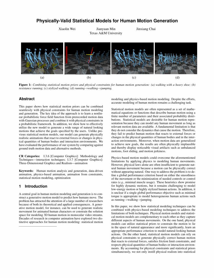
Physically-Valid Statistical Models for Human Motion Generation

Xiaolin Wei Jianyuan MinTexas A&M University

Jinxiang Chai

(a) (b) (c) (d)

Figure 1: Combining statistical motion priors and physical constraints for human motion generation: (a) walking with a heavy shoe; (b)resistance running; (c) stylized walking; (d) running→walking→jumping.

Abstract

This paper shows how statistical motion priors can be combinedseamlessly with physical constraints for human motion modelingand generation. The key idea of the approach is to learn a nonlin-ear probabilistic force field function from prerecorded motion datawith Gaussian processes and combine it with physical constraints ina probabilistic framework. In addition, we show how to effectivelyutilize the new model to generate a wide range of natural lookingmotions that achieve the goals specified by the users. Unlike pre-vious statistical motion models, our model can generate physicallyrealistic animations that react to external forces or changes in phys-ical quantities of human bodies and interaction environments. Wehave evaluated the performance of our system by comparing againstground truth motion data and alternative methods.

CR Categories: I.3.6 [Computer Graphics]: Methodology andTechniques—interaction techniques; I.3.7 [Computer Graphics]:Three-Dimensional Graphics and Realism—animation

Keywords: Human motion analysis and generation, data-drivenanimation, physics-based animation, animation from constraints,statistical motion modeling, optimization

1 Introduction

A central goal in human motion modeling and generation is to con-struct a generative motion model to predict how humans move. Theproblem has attracted the attention of a large number of researchersbecause of both its theoretical and applied consequences. A gener-ative motion model, for instance, can be used to generate realisticmovement for animated human characters or constrain the solutionspace for modeling 3D human motion in monocular video streams.Decades of research in computer animation have explored two dis-tinctive approaches for human motion modeling: statistical motion

modeling and physics-based motion modeling. Despite the efforts,accurate modeling of human motion remains a challenging task.

Statistical motion models are often represented as a set of mathe-matical equations or functions that describe human motion using afinite number of parameters and their associated probability distri-butions. Statistical models are desirable for human motion repre-sentation because they can model any human movement as long asrelevant motion data are available. A fundamental limitation is thatthey do not consider the dynamics that cause the motion. Therefore,they fail to predict human motion that reacts to external forces orchanges in the physical quantities of human bodies and in the inter-action environments. Moreover, when motion data are generalizedto achieve new goals, the results are often physically implausibleand thereby display noticeable visual artifacts such as unbalancedmotions, foot sliding, and motion jerkiness.

Physics-based motion models could overcome the aforementionedlimitations by applying physics to modeling human movements.However, physical laws alone are often insufficient to generate nat-ural human movement because a motion can be physically correctwithout appearing natural. One way to address the problem is to de-fine a global performance criterion based on either the smoothnessof the movement or the minimization of needed controls or controlrates (e.g., minimal muscle usage). These heuristics show promisefor highly dynamic motions, but it remains challenging to modellow-energy motion or highly stylized human actions. In addition, itis unclear if a single global performance objective such as minimaltorque is appropriate to model heterogeneous human actions suchas running→walking→jumping.

In this paper, we show how statistical modeling techniques can becombined with physics-based modeling techniques to address thelimitations of both techniques. Physical motion models and statisti-cal motion models are complementary to each other as they capturedifferent aspects of human movements. On the one hand, physicalmodels can utilize statistical priors to constrain the motion to liein the space of natural appearance and more significantly, learn anappropriate performance criterion to model natural-looking humanactions. On the other hand, statistical motion models can rely onphysical constraints to generate physically correct human motionthat reacts to external forces, satisfies friction limit constraints, andrespects physical quantities of human bodies or interaction environ-ments. By accounting for physical constraints and statistical priorssimultaneously, we not only instill physical realism into statistical

motion models but also extend physics-based modeling to a widevariety of human actions such as stylized walking.

The key idea of our motion modeling process is to learn non-linear probabilistic force field functions from prerecorded motiondata with Gaussian Process (GP) models and combine them withphysical constraints in a probabilistic framework. In our formu-lation, a force field function u = g(q, q) maps kinematic states(joint poses q and joint velocities q) to generalized forces (u). Wedemonstrate the power and effectiveness of our motion model inconstraint-based motion generation. We show that we can cre-ate a natural-looking animation that reacts to changes in physicalparameters such as masses or inertias of human bodies and fric-tion properties of environments (Figure 1(a)) or external forcessuch as resistance forces (Figure 1(b)). In addition, we show thata single physically valid statistical model is sufficient to createphysically realistic animation for a wide range of style variationswithin a particular human action such as “sneaky” walking (Fig-ure 1(c)) or transitions between heterogeneous human actions suchas running→walking→jumping (Figure 1(d)). We evaluate the per-formance of our model by comparing with ground truth data as wellas alternative techniques.

2 Background

We introduce a physically valid statistical motion model that com-bines physical laws and statistical motion priors and use it to createphysically realistic animation that achieves the goals specified bythe user. Therefore, we will focus our discussion on statistical mo-tion modeling and physics-based motion modeling as well as theirapplications in constraint-based motion synthesis.

Statistical models are desirable for human motion modeling andsynthesis because they are often compact and can be used to gen-erate human motions that are not in prerecorded motion data. Thusfar, a wide variety of statistical motion models have been devel-oped; their applications include inverse kinematics [Grochow et al.2004; Chai and Hodgins 2005], human motion synthesis and edit-ing [Li et al. 2002; Chai and Hodgins 2007; Lau et al. 2009; Minet al. 2009], human motion style interpolation and transfer [Brandand Hertzmann 2000; Ikemoto et al. 2009; Min et al. 2010], andso forth. Nonetheless, the motions generated by statistical motionmodels are often physically invalid because existing statistical mo-tion models do not consider the forces that cause the motion. An-other limitation is that they do not react to perturbations (e.g., ex-ternal forces) or changes in physical quantities such as masses andinertias of human bodies.

Physics-based motion models could overcome the limitations ofstatistical motion models by applying physics to modeling humanmovement. However, physics-based motion modeling is a mathe-matically ill-posed problem because there are many ways to adjusta motion so that physical laws are satisfied, and yet only a subset ofmotions are natural-looking. One way to address this limitation isby adopting the “minimal principle” strategy, which was first intro-duced to the graphics community by Witkin and Kass [1988]. Theypostulated that an individual would determine a movement in such away as to reduce the total muscular effort to a minimum, subject tocertain constraints. Therefore, a major challenge in physics-basedmotion modeling is how to define an appropriate performance cri-terion for the “minimal principle.” Decades of research in com-puter animation (e.g., [Witkin and Kass 1988; Cohen 1992; Liuet al. 1994; Fang and Pollard 2003]) introduced numerous perfor-mance criteria for human motion modeling, e.g., minimal energy,minimal torque, minimal jerk, minimal joint momentum, minimaljoint acceleration, or minimal torque change. These heuristics showpromise for highly dynamic motions, but it remains very difficult to

model low-energy motions and highly stylized human movements.

A number of researchers have recently explored the potential of us-ing prerecorded motion data to improve physics-based optimizationmethods, including editing motion data with the help of simplifiedphysical models [Popovic and Witkin 1999], initializing optimiza-tion with reference motion data [Sulejmanpasic and Popovic 2005],learning parameters of motion styles from prerecorded motiondata [Liu et al. 2005], and reducing the search space for physics-based optimization [Safonova et al. 2004; Ye and Liu 2008]. Sim-ilar to these methods, our system utilizes both motion data andphysics for human motion analysis and generation, but there are twoimportant distinctions. First, we rely on statistical motion modelsrather than a predefined global performance objective (e.g., mini-mal muscle usage) to reduce the ambiguity of physics-based mod-eling. This enables us to extend physics-based modeling to stylistichuman motions such as “sneaky walking”. Another attraction ofour model is that it learns the mapping from the kinematic statesto generalized forces using Gaussian process models. Unlike ref-erence trajectories or linear subspace models adopted in previouswork, GP models are capable of modeling both stylistic variationswithin a particular human action and heterogeneous human behav-iors.

Our research draws inspiration from the large body of literature ondeveloping control strategies for physics-based simulation. In par-ticular, our nonlinear probabilistic force field functions are concep-tually similar to control strategies used for physics-based simula-tion because both representations aim to map kinematic states todriving forces. Thus far, researchers in physics-based simulationhave explored two approaches for control design, including man-ually designed control strategies (e.g. [Hodgins et al. 1995]) andtracking a reference trajectory while maintaining balance [Zordanand Hodgins 2002; Sok et al. 2007; Yin et al. 2007; da Silva et al.2008; Muico et al. 2009]. However, our approach is different in thatwe automatically learn nonlinear probabilistic mapping functionsfrom large sets of motion data. In addition, our goal is differentbecause we aim to generate a desired animation that matches userconstraints. Physics-based simulation approaches are not appropri-ate for our task because forward simulation techniques often do notprovide accurate control over simulated motions.

Our approach uses Gaussian process to model a nonlinear prob-abilistic function that maps from kinematic states to generalizedforces. GP and its invariants (e.g., GPLVM) have recently beenapplied to modeling kinematic motion for many problems in com-puter animation, including nonlinear dimensionality reduction forhuman poses [Grochow et al. 2004], motion interpolation [Mukaiand Kuriyama 2005], motion editing [Ikemoto et al. 2009], and mo-tion synthesis [Ye and Liu 2010]. In particular, Ikemoto and hercolleagues [2009] learned the kinematic mapping from pose infor-mation of the source motion to pose and acceleration information ofthe target motion and applied them to transferring a new source mo-tion into a target motion. Ye and Liu [2010] used GPLVM to con-struct a second-order dynamic model for human kinematic data andused them to synthesize kinematic walking motion after a pertur-bation. Our approach is different in that we focus on modeling therelationship between kinematic data and generalized forces ratherthan kinematic motion data itself.

3 Overview

We construct a physically valid statistical model that leverages bothphysical constraints and statistical motion priors and utilize it togenerate physically realistic human motion that achieves the goalsspecified by the user.

Physics-based dynamics modeling. Our motion model considers

Figure 2: Motion data preprocessing for joint pose data (q), joint velocity data (q) and generalized force data (u). (top) before the prepro-cessing; (bottom) after the preprocessing.

both Newtonian dynamics and contact mechanics for a full-bodyhuman figure. Therefore, we describe the Newtonian dynamicsequations for full-body movement and Coulomb’s friction modelfor computing the forces caused by the friction between the charac-ter and the interaction environment (Section 4).

Force field function modeling. We automatically extract forcefield priors from prerecorded motion data (Section 5). Our forcefield priors are represented by a nonlinear probabilistic functionu = g(q, q) that maps the kinematic states (q, q) to the general-ized forces u. To achieve this goal, we precompute the generalizedforces u from prerecorded kinematic motion data and apply Gaus-sian process to modeling the force field priors embedded in trainingdata.

Motion modeling and synthesis. We show how to combine forcefield priors with physics-based dynamics models seamlessly in aprobabilistic framework and how to use the new motion model togenerate physically realistic animation that matches user-definedconstraints (Section 6). We formulate the constraint-based motionsynthesis problem in a Maximum A Posteriori (MAP) frameworkand introduce an efficient gradient-based optimization algorithm tofind an optimal solution.

4 Physics-based Dynamics Models

Our dynamics models approximate human motion with a set ofrigid body segments. We describe a full-body character pose witha set of independent joint coordinates q ∈ R48, including abso-lute root position and orientation, and the relative joint angles of 18joints. These joints are the head, thorax, upper neck, lower neck,upper back, lower back, left and right humerus, radius, wrist, femur,tibia, and metatarsal.

Newtonian dynamics. The Newtonian dynamics equations forfull-body movement can be described using the following equa-tion [Jazar 2007]:

M(q)q + C(q, q) + h(q) = τ + fc + fe ≡ u (1)

where q, q, and q represent the joint angle poses, joint velocities,and joint accelerations, respectively. The quantities M(q), C(q, q)and h(q) are the joint space inertia matrix, centrifugal/Coriolis andgravitational forces, respectively. The vectors τ , fc, and fe representjoint torques, contact forces, and external forces, respectively. Thevector u represent the generalized forces, which can be either calcu-lated from kinematic data or resultant forces of join torques, contactforces, and external forces. Human muscles generate torques about

each joint, leaving global position and orientation of the body as un-actuated joint coordinates. As a result, the movement of the globalposition and orientation is completely determined by contact forcesfc and external forces fe.

Contact mechanics. During ground contact, the feet can onlypush but not pull on the ground. To keep the body balanced, con-tact forces should not require an unreasonable amount of frictionand the center of pressure must fall within the support polygon ofthe feet. We use Coulomb’s friction model to compute the forcescaused by the friction between the character and the environment.A friction cone is defined to be the range of possible forces satisfy-ing Coulomb’s function model for an object at rest.

We ensure the contact forces stay within a basis that approximatesthe cones with nonnegative basis coefficients. We model the contactbetween two surfaces with multiple contact points m = 1, ...,M .As a result, we can represent the contact forces fc as a function ofthe joint angle poses and nonnegative basis coefficients [Pollard andReitsma 2001; Liu et al. 2005]:

fc(q, λ) =

M∑m=1

Jm(q)TBmeλm (2)

where the matrix Bm is a 3 × 4 matrix consisting of 4 basis vec-tors that approximately span the friction cone for the m-th contactforce. The 4 × 1 vector eλm represents nonnegative basis weightsfor the m-th contact force. The contact force Jacobian Jm(q) mapsthe instantaneous generalized joint velocities to the instantaneousworld space cartesian velocities at the m-th contact point under thejoint pose q. Note that we remove the nonnegative coefficients con-straints by representing the basis weights with exponential func-tions.

Enforcing Newtonian dynamics equations and friction limit con-straints would allow us to generate physically correct motion thatsatisfies friction limit constraints. However, physical constraintsalone are insufficient to model natural-looking human movementbecause a motion can be physically correct without appearing natu-ral. In the next section, we discuss how to learn force field functionsfrom prerecorded motion data to constrain the human motion to liein the space of natural appearance.

5 Force Field Function Modeling

Our system automatically extracts force field priors embedded inprerecorded motion data. Our idea of force field modeling is moti-

(a) (b) (c)

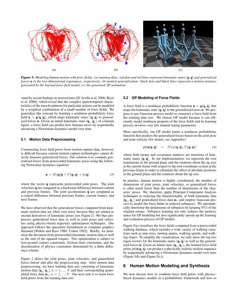
Figure 3: Modeling human motion with force fields: (a) training data: red dots and red lines represent kinematic states [q, q] and generalizedforces u in the two-dimensional eigenspace, respectively; (b) motion generalization: black dots and black lines represent a motion instancegenerated by the learned force field model; (c) the generated 3D animation.

vated by recent findings in neuroscience [D’Avella et al. 2006; Bizziet al. 2008], which reveal that the complex spatiotemporal charac-teristics of the muscle patterns for particular actions can be modeledby a weighted combination of a small number of force fields. Wegeneralize this concept by learning a nonlinear probabilistic forcefield u = g(q, q), which maps kinematic states (q, q) to general-ized forces u. Given an initial kinematic state (q1, q1) of a humanfigure, a force field can predict how humans move by sequentiallyadvancing a Newtonian dynamics model over time.

5.1 Motion Data Preprocessing

Constructing force field priors from motion capture data, however,is difficult because current motion capture technologies cannot di-rectly measure generalized forces. Our solution is to compute gen-eralized forces from prerecorded kinematic poses using the follow-ing Newtonian dynamics equation:

u = M(q)q + C(q, q) + h(q) (3)

where the vector q represents prerecorded joint poses. The jointvelocities q are computed as a backward difference between currentand previous frames. The joint accelerations q are computed asa central difference between previous frames, current frames, andnext frames.

We have observed that the generalized forces computed from kine-matic motion data are often very noisy because they are related tosecond derivatives of kinematic poses (see Figure 2). We thus pre-process generalized force data as well as joint poses and veloci-ties using physics-based trajectory optimization techniques. Ourapproach follows the spacetime formulation in computer graphicsliterature [Witkin and Kass 1988; Cohen 1992]. Briefly, we mini-mize the deviation from prerecorded kinematic motion data as wellas the sum of the squared torques. This optimization is subject tofoot-ground contact constraints, friction limit constraints, and thediscretization of physics constraints determined by a finite differ-ence scheme.

Figure 2 shows the joint poses, joint velocities, and generalizedforces before and after the preprocessing step. After motion datapreprocessing, we have training data sets consisting of kinematicmotion data [qn, qn], n = 1, ..., N and their corresponding gener-alized force data un, n = 1, ..., N . Our next task is to learn forcefield priors from the training data sets.

5.2 GP Modeling of Force Fields

A force field is a nonlinear probabilistic function u = g(q, q) thatmaps the kinematic state (q, q) to the generalized forces u. We pro-pose to use Gaussian process model to construct a force field fromthe training data sets. We choose GP model because it can effi-ciently model nonlinear property of the force fields and its learningprocess involves very few manual tuning parameters.

More specifically, our GP model learns a nonlinear probabilisticfunction that predicts the generalized forces based on the joint poseand joint velocity (for details, see Appendix):

pr(u|q, q) = N (µ(q, q),Σ(q, q)) (4)

where both means and covariance matrices are functions of kine-matic states [q, q]. In our implementation, we represent the roottranslations in the ground plane and the rotations about the up axisat the current frame with respect to the root coordinate system at theprevious frame in order to eliminate the effect of absolute positionsin the ground plane and the rotations about the up axis.

In practice, human motion is highly coordinated, the number ofdimensions of joint poses, joint velocities, or generalized forcesis often much lower than the number of dimensions of the char-acter’ poses. We, therefore, apply Principal Component Analysistechniques to reducing the dimensionality of both kinematic data[qn, qn] and generalized force data un and employ Gaussian pro-cess to model the force fields in reduced subspaces. We automati-cally determine the dimensions of subspaces by keeping 95% of theoriginal energy. Subspace learning not only reduces the memoryspace for GP modeling but also significantly speeds up the learningand evaluation process of GP models.

Figure 3(a) visualizes the force fields computed from a prerecordedwalking database, which includes a wide variety of walking varia-tions such as step sizes, turning angles, walking speeds, and walk-ing slopes. To simplify the visualization, we only show the top twoeigen-vectors for the kinematic states (q, q) as well as the general-ized forces u. Given an initial state (q1, q1), the learned force fieldpriors pr(u|q, q) can produce a physically realistic motion sequenceby sequentially advancing a Newtonian dynamics model over time(Figure 3(b) and Figure 3(c)).

6 Human Motion Modeling and Synthesis

We now discuss how to combine force field priors with physics-based dynamics models in a probabilistic framework and how to

apply the proposed framework to generating physically realistic hu-man motion that achieves the goals specified by the user.

6.1 Combining Physics with Statistical Priors

We introduce a probabilistic motion model to model how humansmove. Let pr(x) represent a probabilistic model of human mo-tion x = {(qt, qt, ut)|t = 1, ..., T}, where qt, qt, and ut are jointposes, joint velocities, and generalized forces at frame t, respec-tively.

According to Bayes’ rule, we can decompose the probabilistic mo-tion model pr(x) into the following three terms:

pr(x) = pr(q1, q1)︸ ︷︷ ︸ ·∏tpr(ut|qt, qt)︸ ︷︷ ︸ · pr(qt+1, qt+1|qt, qt, ut)︸ ︷︷ ︸

prinit prforcefield prphysics(5)

where the first term prinit represents the probabilistic density func-tion of the initial kinematic pose and velocity. In our experiment,we model the initial kinematic priors prinit with Gaussian mixturemodels. The second term prforcefield represents the force field pri-ors described in Equation (4).

The third term prphysics measures how well the generated motionsatisfies the physical constraints. In order to evaluate the third termprphysics, we first use backward difference to compute joint veloci-ties and use central difference to compute joint accelerations. Basedon the dynamics equation defined in Equation (1), the joint pose,joint velocities and generalized forces in the current step shouldcompletely determine the joint accelerations in the current step.Therefore, the joint pose and velocity in the next frame are alsofully determined due to finite difference approximation.

Mathematically, we have

prphysics = pr(qt+1, qt+1|qt, qt, ut)∝ pr(qt|qt, qt, ut) (6)

In practice, as noted by other researchers [Sok et al. 2007; Muicoet al. 2009], dynamics models adopted in physics-based modelingare often inconsistent with observed data because of simplified dy-namics/contact models, discretization of physics constraints, andapproximate modeling of physical quantities of human bodies suchas masses and inertias. Accordingly, dynamics equations are oftennot satisfied precisely. In our formulation, we assume Newtoniandynamics equations are disturbed by Gaussian noise of a standarddeviation of σphysics:

prphysics ∝ pr(qt|qt, qt, ut)∝ exp

−‖M(qt)qt+C(qt,qt

)+h(qt)−τt−fc(qt,λt)−fe‖22σ2

physics

(7)where the standard deviation σphysics shows our confidence ofphysics-based dynamics models. If the standard deviation is small,then the Gaussian probability distribution has a narrow peak, indi-cating high confidence in the physical constraints; similarly, a largestandard deviation indicates low confidence.

Such a motion model would allow us to generate an infinite num-ber of physically realistic motion instances. In particular, we cansample the initial prior distribution prinit to obtain an initial statefor joint poses and velocities and sequentially predict joint torquesusing the force field priors prforcefield to advance the Newtoniandynamics model prphysics over time. More importantly, we canemploy the motion model pr(x) to generate physically realistic an-imation x that best matches the user’s input c.

6.2 Constraint-based Motion Synthesis

We formulate the constraint-based motion synthesis problem in amaximum a posteriori (MAP) framework by estimating the mostlikely motion x from the user’s input c:

arg maxx pr(x|c) = arg maxxpr(c|x)pr(x)

pr(c)∝ arg maxx pr(c|x)pr(x)

(8)

In our implementation, we minimize the negative logarithm of theposteriori probability density function pr(x|c), yielding the follow-ing energy minimization problem:

arg minx − ln pr(c|x)︸ ︷︷ ︸ + − ln pr(x)︸ ︷︷ ︸,Ec Eprior

(9)

where the first term Ec is the likelihood function measuring howwell the generated motion x matches the input constraints c. Simi-lar to [Chai and Hodgins 2007], the system allows the user to spec-ify various forms of kinematic constraints throughout the motionor at isolated points in the motion. Typically, the user can define asparse set of key frames as well as contact constraints to generate adesired animation. The user could also specify a small number ofkey trajectories to control fine details of a particular human actionsuch as stylized walking. The second term Eprior is the prior dis-tribution function defined by our physically valid statistical modelin Equation (5).

The motion synthesis problem can now be solved by nonlinear op-timization methods. Given a sparse set of constraints c, the opti-mization computes joint poses, joint torques, and contact forces byminimizing the following objective function:

argmin{qt,τt,λt} ω1Ec + ω2Einit + ω3Eforcefield+ω4Ephysics

(10)

where Einit, Eforcefield, and Ephysics are the negative log ofprinit, prforcefield, and prphysics, respectively. In our experiment,we set the weights forEc,Einit,Eforcefield andEphysics to 1000,1, 1 and 100, respectively1. We choose a very large weight for theconstraint term because we want to ensure the generated motioncan match user constraints accurately. The weight for the physicalterm is much larger than the statistical prior term because physicalcorrectness has a higher priority than statistical consistency in oursystem.

Thus far, we have not discussed how to incorporate the learnedforce field priors into the motion optimization framework. Notethat in the force field modeling step, we performed dimensional-ity reduction analysis on both kinematic data and generalized jointtorques and learned the force field priors in reduced subspaces. Onepossible solution to incorporating the force field priors is to performthe optimization in the reduced subspaces. We have implementedthis idea and found that performing the optimization in the sub-spaces can hurt the generalization ability of our model and oftencannot match user-specified constraints accurately. To avoid thisissue, we choose to perform the optimization in the original config-uration space while imposing “soft” subspace constraints on bothkinematic states and generalized forces.

Let Bu and Bs denote the subspace matrices for generalized forcesu and kinematic states s = [qT , qT ]T , respectively. We reformulate

1Note that the weight for the physics term (ω4) corresponds to1

2σ2physics

in Equation 7

Motion examples Total frames Durations Total key frames Total key trajectories Initialization times Synthesis timesNormal walking 270 9s 2 0 9 sec 17 minBig-step walking 272 9s 2 0 7 sec 16 min

Walking and turning 392 13s 2 0 10 sec 20 minRunning 130 4.3s 2 0 5 sec 10 minJumping 168 5.6s 3 0 3 sec 7 min

Heavy foot 235 7.8s 2 0 10 sec 22 minResistance running 148 4.9s 2 0 5 sec 13 minSlippery surfaces 193 6.4s 2 0 8 sec 20 min

Moon walking 193 6.4s 2 0 8 sec 21 minSneaky walking 674 22.5s 2 3 20 sec 23 minProud walking 302 10.1s 2 2 12 sec 16 min

Long walking sequence 1357 45.2s 8 0 27 sec 51 minRun→walk→jump 510 17s 6 2 13 sec 21 min

Table 1: Details of all the animations generated by our synthesis algorithm.

Databases size Durations Prep. GP learningwalking 5227 2.9 min 65 min 40 min

stylized walking 7840 4.4 min 138 min 46 minlocomotion 4571 2.5 min 55 min 47 min

Table 2: Details of three training data sets and the computationaltimes spent on data preprocessing (Section 5.1) and GP learning(Section 5.2).

the force field priors as follows:

− ln pr(BTu u|BTs s) + α1‖u−BuBTu u‖2 + α2‖s−BsBTs s‖2︸ ︷︷ ︸Eforcefield

(11)where the first term represents the force field priors in reduced sub-spaces. The second and third terms impose the “soft” subspaceconstraints for kinematic states and generalized forces, penalizingthem as they deviate from the subspace representations. In our ex-periment, we set the weights α1 and α2 to 10 and 10, respectively.

The combined motion models are desirable for human motion gen-eration because they measure both statistical consistency and phys-ical correctness of the motion. With the physical term, our modelcan react to changes in physical parameters. For example, when acharacter is pushed by an external force, e.g., elastic forces in re-sistance running, the external force in the physics term Ephysics(see Equation 7) will force the system to modify kinematic motionand joint torques as well as contact forces in order to satisfy New-tonian dynamics and contact mechanics. However, without forcefield priors, the modified motion could be unnatural because thereare many ways to adjust a motion so that physical laws are satis-fied, and yet only a subset of motions are natural-looking. Withforce field priors, our system pushes the modified motions towardsregions of high probability density in order to be consistent withforce field priors.

7 Implementation Details

Here we briefly discuss implementation details of our system:

Data preprocessing. We used three different motion databases inour experiments, including walking (5227 frames), stylized walking(7840 frames), and locomotion databases (4571 frames). We pre-processed the prerecorded motion data using spacetime optimiza-tion (Section 5.1). The computational time for each data set wasreported in Table 2.

GP learning. To speed up the learning and evaluation process ofGP models, we applied PCA to reduce the dimensionality of train-ing data and learned the GP model in a reduced subspace. We auto-matically determined the dimension of the subspace by preserving95% of the original energy. The dimensions of the kinematic states([qt, qt]) in three databases were 19, 22, and 19 respectively. Thedimensions of the generalized forces (u) were 8, 10, and 7 respec-tively. We adopted sparse approximation strategies for Gaussianprocess modeling [Quinonero-Candela and Rasmussen 2005]. TheGP learning times spent on the three training databases were 65minutes, 138 minutes, and 55 minutes, respectively.

Motion optimization. We follow a standard approach of represent-ing qt and τt using cubic B-splines. We solved the optimizationproblem using sequential quadratic programming (SQP) [Bazaraaet al. 1993], where each iteration solves a quadratic programmingsubproblem. We implemented the system with C++/Matlab andconducted the optimization with the Matlab optimization toolbox.Each optimization often took from ten to thirty minutes to convergewithout code optimization (for details, see Table 1). All the ex-periments were run on a 2.5GHz dual core computer with 3GB ofRAM.

Initialization. The performance of our optimization algorithmhighly depends on the initialization of the optimization. To obtaina good initial guess for joint poses qt, t = 1, ..., T , we droppedoff the physical term Ephysics in the objective function and usedthe remaining objective functions to optimize the joint poses acrossthe entire motion sequence. We evaluated the force field termwith respect to joint poses because we can calculate current gen-eralized forces using current joint poses, velocities and accelera-tions as shown in Equation (3). With the initialized joint posesqt0, t = 1, ..., T , we dropped off the constraint term as well as theinitial prior term, and optimized the joint torques τ as well as con-tact forces λ using the force field prior term and the physics term. Inthis step, we evaluated the force field priors in terms of joint torquesand contact forces: Eforcefield(τ, λ) = − ln pr(τ + fc(q0, λ) +fe)|q0, q0). Each initialization step often took from less than thirtyseconds to converge (for details, see Table 1).

8 Experiments

This section demonstrated the benefits of combining physical con-straints and statistical motion priors for human motion generation.In addition, we evaluated the performance of our algorithm by com-paring with ground truth data and results obtained by alternativemethods. The details for our experiments are summarized in Ta-ble 1. For each example in our experiments, we reported the total

Figure 4: Generating physically realistic motion that reacts to changes in physical quantities of human bodies: walking with a heavy leftfoot.

number of animation frames, the types and number of animationconstraints, and the computational times spend on the initializationand motion synthesis step.

8.1 The Benefits of Physical Constraints

The incorporation of physics into probabilistic motion models sig-nificantly improves the generalizability of statistical motion mod-els. This experiment shows that the system can generate physicallyrealistic motion that reacts to changes in physical quantities of hu-man bodies and interaction environments, a capability that has notbeen demonstrated in previous statistical motion models.

Heavy foot. Our system can react to changes in physical quanti-ties such as masses and inertias of human bodies. For example, wechanged the mass of the character by simulating a character wear-ing a 2.5 kilogram shoe. The accompanying video shows that thesimulated character maintained balance by adapting the gait andleaning the body to the right side in order to offset the additionalweigh caused by the left shoe. Figure 4 shows sample frames forwalking with a heavy foot.

Resistance running. In this example, the user specified the startand end poses as well as foot contacts to create an animation forresistance running (Figure 1(b)). The resistance forces were deter-mined by Hooke’s law of elasticity, ranging from zero to 450N. Weobserved that the character moved the upper body forward in orderto offset the effect of resistance force.

Walking on slippery surfaces. We can generate an animation thatreacts to changes in friction properties of environments. In the ac-companying video, we show a simulated character walking on aslippery surface by reducing the friction coefficient to 0.05.

Moon walking. We can edit an animation by changing the gravityof interaction environments. For example, we generated “moon”walking by setting gravity at 1.62 m/s2.

8.2 The Benefits of Statistical Motion Priors

This experiment shows that we can extend physics-based modelingtechniques to stylized walking, detailed walking variations, and het-erogeneous human actions with the help of statistical motion priors.Such actions are often difficult or even impossible to generate withprevious physics-based modeling techniques.

Stylized walking. Our approach can generate physically-realisticanimation for highly stylized human actions. The training data setsfor stylized walking included normal walking and ten distinct walk-ing styles. The system constructed a single motion model fromthe training data sets and used it to generate various forms of styl-ized walking such as “sneaky” walking and “proud” walking (Fig-ure 1(c)). In addition to keyframes and foot contact constraints, the

user specified a sparse number of key trajectories in order to controlthe fine details of stylized walking.

Walking variations. We tested the effectiveness of our algorithmfor modeling a wide range of walking variations. We learned a sin-gle generative model from a “walking” database and used it to gen-erate a long walking sequence. The synthesized motion displayed awide variety of walking variations such as walking along a straightline, walking with a sharp turn, walking with a big step, walkingon a slope, climbing over an obstacle, and transitionings betweendifferent walking examples (Figure 5). Because of memory restric-tions, we synthesized the whole motion sequence by sequentiallycomputing each example from sparse constraints and stitching theminto a long motion sequence. For each example, the user specifiedthe start and end poses of the generated motion as well as foot con-tact constraints throughout the whole motion sequence.

Heterogeneous actions. We tested the effectiveness of the physi-cally valid statistical model on heterogeneous human actions. Welearned a single generative model from a locomotion database andused it to create a long animation sequence consisting of walking,running, jumping, and stopping, as well as their transitions (Fig-ure 1(d)).

8.3 Evaluation and Comparisons

We assessed the quality of the generated motions by comparingwith ground truth data. We also evaluated the importance of forcefield priors and physical constraints for human motion generation.

Comparison against ground truth data. We evaluated the per-formance of our algorithm via cross validation techniques. Morespecifically, we pulled out a testing sequence in the training data,used it to extract the start and end poses and foot contact con-straints, and applied the synthesis algorithm to generate motionthat matches the “simulated” constraints. The accompanying videoshows a side-by-side comparison between the ground truth motionand the synthesized motion. We have observed that the generatedmotions achieve similar quality to the ground truth motion data.

The importance of force field priors. This comparison showsthe importance of force field priors for human motion generation.We compared our system with standard physics-based optimizationtechniques [Witkin and Kass 1988] by dropping off both force fieldpriors term Eforcefield and initialization term Einit in the objec-tive function defined in Equation (10). For a fair comparison, weadded the minimal sum of squared joint torques into the objectivefunction because optimizing the motion with the remaining terms(Ec and Ephysics) is ambiguous–there are an infinite number ofphysically correct motions that satisfy user constraints. We also in-cluded joint torque limits into the optimization. Without the forcefield priors, the “sneaky” walking appears ballistic because the

(a) (b) (c) (d)

Figure 5: Generating a wide variety of physically realistic walking motions: (a) normal walking; (b) walking with a big step; (c) climbingover an obstacle; (d) walking on a slope. All the motions are generated by a single statistical walking model constructed from a prerecordedwalking database

“minimal torque principle” is not suitable for stylized low-energymotion. With the force field priors, our system can successfullygenerate physically realistic stylized walking motion.

(a) (b)

Figure 6: The importance of the physics term. (a) with the physicsterm; (b) without the physics term. Note that with the physics term,the simulated character reacts to external elastic forces by leaningthe body forward to compensate the resistance forces. Note that“yellow” characters are the starting and ending keyframes used formotion generation; foot contact constraints as shown in “green”.

The importance of the physics term. This experiment demon-strated the importance of physical constraints to our motion model.We dropped off the physics term in the objective function and usedthe remaining terms to optimize the joint poses across the entire mo-tion sequence. The accompanying video shows a side-by-side com-parison for animating the “resistance running”. With the physicsterm, the character reacted appropriately to external elastic forcesby leaning the body forward to compensate for the resistance forces(Figure 6(a)). As expected, the character did not respond to externalforces without the physics term (Figure 6(b)).

Comparison against subspace optimization. We computedthe eigen-poses using the same set of training data and per-formed physics-based optimization in a reduced eigen-space sim-ilar to Safonova and her colleagues [2004]. The testing examplewas running→walking→jumping. Unlike Safonova and her col-leagues [2004], we did not manually select training data to constructa reduced subspace for human poses. Instead, we used the entire lo-comotion database (4571 frames), which includes normal walking,running and jumping. We automatically determined the dimensionof the subspace (11 dimensions) by preserving 95% of energy ofthe training data.

To implement the subspace optimization algorithm, we formulatedthe problem in the spacetime framework and optimized the motionin the reduced subspace. Briefly, we minimized the sum of squaredtorques and smoothness of the root and joint angle trajectories overtime. We also added a regularization term to penalize the deviationof eigen coefficients from zero. This optimization was also subject

to foot-ground contact constraints, friction limit constraints, and thediscretization of physics constraints determined by a finite differ-ence scheme. Unlike Safonova and her colleagues [2004], we didnot incorporate inverse kinematics as part of optimization in ourimplementation.

We evaluated the performance of the subspace optimization tech-nique using the same set of animation constraints, including thestart and end poses as well as trajectories of the head and two feet.The accompanying video shows that subspace optimization pro-duces uncoordinated human movements. For example, the walkingcharacter did not swing the right arm properly and the walking gaitappeared very stiff. This indicates that a global subspace modelfor kinematic poses is not sufficient to model heterogeneous hu-man actions. We have also observed that the motions generated bysubspace methods often cannot accurately match the trajectory andcontact constraints specified by the user; this might be due to com-pression errors caused by reduced subspace representation. In con-trast, the GP-based statistical motion priors can accurately modelspatial-temporal patterns in heterogeneous human actions and al-low for generating physically realistic animation that matches user-defined constraints.

9 Discussion and Future Work

We introduce a statistical motion model for human motion analysisand generation. Our model combines the powers of physics-basedmotion modeling and statistical motion modeling. We have demon-strated the effectiveness of the new model by generating a wide va-riety of physically realistic motions that achieve the goals specifiedby the users.

The incorporation of physical constraints into statistical mo-tion models ensures generalized motions are physically plausible,thereby removing noticeable visual artifacts (e.g., unbalanced mo-tions and motion jerkiness) in an output animation. Moreover, itenables us to create motions that react to changes in physical pa-rameters. In our experiments, we have shown that the system cangenerate new motions such as “resistance running”, “moon walk-ing”, “walking on slippery surfaces”, and “walking with a heavyfoot”, a capability that has never been demonstrated in any previ-ous statistical motion synthesis methods.

Meanwhile, the use of force field priors for human motion model-ing not only ensures that generated motions are natural looking butalso extends physically-based modeling techniques to stylized andheterogeneous human actions. For example, we have constructeda single generative model for modeling a wide variety of physi-cally realistic walking variations such as normal walking, walkingwith a sharp turn, walking on a slope, walking with a big step, andclimbing over an obstacle. We have also shown that the system

can generate physically realistic motion for stylized walking suchas sneaky walking and for heterogeneous human actions such asrunning→walking→jumping. Such actions are often difficult oreven impossible to be synthesized by previous physics-based mo-tion models.

We model the force field priors using Gaussian process models be-cause GP can efficiently capture nonlinear properties of the forcefields and its learning process involves very few manual tuning pa-rameters. However, Gaussian process needs to retain all of thetraining data to make predictions and therefore its computationaldemands grow as the square and cube respectively of the number oftraining examples. The sparse approximation strategy works wellfor the current size of training data sets (less than 8,000 frames)but might not scale up for use in very large data sets. One possi-bility is to learn a probabilistic regression function for force fieldsusing parametric statistical analysis techniques such as the mixtureof experts model [Jacobs et al. 1991] or its variants [Jordan 1994].Another limitation of our system is that it cannot generate a motionthat is very different from motion examples because our approachis data-driven. In addition, the system is still unable to handle arbi-trary external forces because the force field priors prevent the gen-erated motion from moving away from prerecorded motion data.

We choose to model the force field priors based on generalizedforces rather than joint torques because we can conveniently com-pute the generalized forces from current kinematic motion capturedatabases (e.g., the CMU online mocap database2). However, thelearned force field priors can only predict resultant forces of jointorques and contact forces. If both joint torque data and contactforce data are available, we could construct more accurate forcefield priors that explicitly predict joint torques or contact forces. Inthe future, we plan to measure ground-reaction forces with forceplates and use them along with the captured kinematic motion datato compute joint torques via inverse dynamics techniques.

We formulate the constraint-based motion synthesis problem ina spacetime optimization framework. However, the optimizationproblem is high-dimensional and highly nonlinear; it might be sub-ject to local minima. We found that the initialization process iscritical to the success of our optimization. It not only speeds up theoptimization process but also alleviates the local-minimum prob-lem. For a long sequence of animation (e.g., Figure 5), we needto decompose the entire optimization into a number of spacetimewindows, over which subproblems can be formulated and solvedusing efficient nonlinear optimization techniques. In the future, weplan to explore alternative techniques to address the local minimumproblem. One possibility is the employment of a Markov chainMonte Carlo (MCMC), which comes to its solutions by efficientlydrawing samples from the posterior distribution, using a Markovchain based on the Metropolis-Hastings algorithm.

Similar to other constraint-based animation systems, our system re-quires the user to specify a sparse number of constraints, e.g., keyframes and contact constraints, to generate a desired animation.However, specifying such constraints, particularly trajectory con-straints and contact constraints, is not trivial for a novice user. Inour experiment, we created the 3D key frames by using our home-grown data-driven inverse kinematic system [Wei and Chai 2010a].Trajectory and contact constraints were either directly modifiedfrom reference motion data or rotoscoped from video streams sim-ilar to the technique described by Wei and Chai [2010b]. In thefuture, we are interested in extending our system to searching thepositions and timings of contact events as part of the optimizationvariables, thereby avoiding the necessity of contact constraints re-quired for constraint-based motion synthesis.

2http://mocap.cs.cmu.edu/

APPENDIX

A Gaussian Processes

Gaussian processes (GP) are a powerful, non-parametric tool forregression in high-dimensional space. A GP can be thought of asa “Gaussian over functions”. Here, we briefly discuss the basicconcept of Gaussian processes.

Let D = {(yn, zn)|n = 1, ..., N} be the training set. For our ap-plication, we have y = [q, q] and z = u. The goal of Gaussianprocesses is to learn a regression function f(·) that finds the pre-dictive output z∗ using a testing input y∗. We assume both trainingand testing data points are drawn from the following noisy process:

zn = f(yn) + ε (12)

where yn is an input vector inRd and zn is a scalar output inR. Thenoise term ε is drawn from N(0, σ2). For convenience, the inputsare stacked into a d×N matrix Y = [y1, y2, ..., yN ] and the outputsare stacked into a N -dimensional vector z = [z1, z2, ..., zN ].

The joint distribution over the noisy output z given inputs Y is azero-mean Gaussian, and has the form

pr(z|Y ) = N(0,K(Y, Y ) + σ2nI), (13)

where K(Y, Y ) is the kernel matrix with elements Kij =k(yi, yj). The kernel function, k(y, y′), is a measure of the “close-ness” between inputs. The term σ2

nI introduces Gaussian noise andplays a similar role to that of ε in Equation (12).

Given a set of test inputs Y∗, one would like to find the predictiveoutput z∗. The noisy training outputs z and the test output z∗ arejointly Gaussian:

pr(z∗, z|Y∗, Y ) = N (0,[K(Y∗, Y∗) K(Y∗, Y )K(Y, Y∗) K(Y, Y ) + σ2

nI

])

(14)Since z is known, this Gaussian can be conditioned on z to obtainthe predictive distribution for z∗:

pr(z∗|z, Y∗, Y ) = N (µ,Σ), (15)

where

µ = K(Y∗, Y )[K(Y, Y ) + σ2nI]−1z,

Σ = K(Y∗, Y∗)−K(Y∗, Y )[K(Y, Y ) + σ2nI]−1K(Y, Y∗).

(16)A Gaussian process is fully described by its mean and covariancefunctions. These equations show that the mean function for the test-ing output is a linear combination of the training output z, and theweight of each input is directly related to the correlation betweenthe testing input Y∗ and the training input Y . Meanwhile, the uncer-tainty for every predictive output (i.e. covariance function) is alsoestimated.

In this paper, we choose the squared exponential function as ourkernel function:

k(y, y′) = σ2f exp−(

1

2(y− y′)TW (y− y′)) (17)

where σ2f is the signal variance. The diagonal matrix W contains

the length scales for each input dimension. The value of Wii is in-versely proportional to the importance of the i-th input dimension.The parameters of the kernel function θ = [W,σf , σn] can be auto-matically learned by maximizing the log likelihood of the trainingoutputs given the inputs: θmax = arg maxθ log pr(z|Y, θ).

References

BAZARAA, M. S., SHERALI, H. D., AND SHETTY, C. M. 1993.Nonlinear Programming: Theory and Algorithms. John Wileyand Sons Ltd. 2nd Edition.

BIZZI, E., CHEUNG, V. C. K., D’AVELLA, A., SALTIEL, P., ANDTRESCH, M. 2008. Combining Modules for Movement. InBrain Research Reviews. 57:125-133.

BRAND, M., AND HERTZMANN, A. 2000. Style Machines. InProceedings of ACM SIGGRAPH 2000. 183–192.

CHAI, J., AND HODGINS, J. 2005. Performance Animationfrom Low-dimensional Control Signals. In ACM Transactionson Graphics. 24(3):686–696.

CHAI, J., AND HODGINS, J. 2007. Constraint-based Motion Opti-mization Using A Statistical Dynamic Model. In ACM Transac-tions on Graphics. 26(3): Article No.8.

COHEN, M. F. 1992. Interactive Spacetime Control for Animation.In Proceedings of ACM SIGGRAPH 1992. 293–302.

DA SILVA, M., ABE, Y., AND POPOVIC, J. 2008. Interactivesimulation of stylized human locomotion. ACM Transactions onGraphics. 27(3): Article No. 82.

D’AVELLA, A., AMD L. FERNANDEZ, A. P., AND LACQUANITI,F. 2006. Control of Fast-reaching Movements by Mus-cle Synergy Combinations. In The Journal of Neuroscience.26(30):7791–7810.

FANG, A., AND POLLARD, N. S. 2003. Efficient Synthesisof Physically Valid Human Motion. In ACM Transactions onGraphics. 22(3):417–426.

GROCHOW, K., MARTIN, S. L., HERTZMANN, A., ANDPOPOVIC, Z. 2004. Style-based Inverse Kinematics. In ACMTransactions on Graphics. 23(3):522–531.

HODGINS, J. K., WOOTEN, W. L., BROGAN, D. C., ANDO’BRIEN, J. F. 1995. Animating Human Athletics. In Pro-ceedings of ACM SIGGRAPH 1995. 71-78.

IKEMOTO, L., ARIKAN, O., AND FORSYTH, D. 2009. Generaliz-ing motion edits with gaussian processes. ACM Transactions onGraphics. 28(1):1–12.

JACOBS, R., JORDAN, M. I., NOWLAN, S. J., AND HINTON,G. E. 1991. Adaptive mixtures of local experts. In NeuralComputation. 2:79-87.

JAZAR, R. N. 2007. In Theory of Applied Robotics: Kinematics,Dynamics, and Control, Springer.

JORDAN, M. I. 1994. Hierarchical mixtures of experts and the emalgorithm. Neural Computation. 6:181–214.

LAU, M., BAR-JOSEPH, Z., AND KUFFNER, J. 2009. ModelingSpatial and Temporal Variation in Motion Data. In ACM Trans-actions on Graphics. 28(5): Article No. 171.

LI, Y., WANG, T., AND SHUM, H.-Y. 2002. Motion Texture:A Two-level Statistical Model for Character Synthesis. In ACMTransactions on Graphics. 21(3):465–472.

LIU, Z., GORTLER, S. J., AND COHEN, M. F. 1994. HierarchicalSpacetime Control. In Proceedings of ACM SIGGRAPH 1994.35–42.

LIU, K., HERTZMANN, A., AND POPOVIC, Z. 2005. LearningPhysics-Based Motion Style with Nonlinear Inverse Optimiza-tion. In ACM Transactions on Graphics. 23(3):1071–1081.

MIN, J., CHEN, Y.-L., AND CHAI, J. 2009. Interactive genera-tion of human animation with deformable motion models. ACMTransactions on Graphics. 29(1): Article No. 9.

MIN, J., LIU, H., AND CHAI, J. 2010. Synthesis and editingof personalized stylistic human motion. ACM Symposium onInteractive 3D Graphics and Games.

MUICO, U., LEE, Y., POPOVIC, J., AND POPOVIC, Z. 2009.Contact-aware Nonlinear Control of Dynamic Characters. ACMTransactions on Graphics. 28(3): Article No. 81.

MUKAI, T., AND KURIYAMA, S. 2005. Geostatistical MotionInterpolation. In ACM Transactions on Graphics. 24(3):1062–1070.

POLLARD, N., AND REITSMA, P. 2001. Animation of Human-like Characters: Dynamic Motion Filtering with A PhysicallyPlausible Contact Model. In In Yale Workshop on Adaptive andLearning Systems.

POPOVIC, Z., AND WITKIN, A. P. 1999. Physically Based MotionTransformation. In Proceedings of ACM SIGGRAPH 1999. 11-20.

QUINONERO-CANDELA, J., AND RASMUSSEN, C. E. 2005. Aunifying view of sparse approximate gaussian process regres-sion. Journal of Machine Learning Research. 6:1935–1959.

SAFONOVA, A., HODGINS, J., AND POLLARD, N. 2004. Synthe-sizing Physically Realistic Human Motion in Low-Dimensional,Behavior-Specific Spaces. In ACM Transactions on Graphics.23(3):514–521.

SOK, K. W., KIM, M., AND LEE, J. 2007. Simulating biped be-haviors from human motion data. ACM Transactions on Graph-ics. 26(3): Article No. 107.

SULEJMANPASIC, A., AND POPOVIC, J. 2005. Adaptation ofPerformed Ballistic Motion. In ACM Transactions on Graphics.24(1):165–179.

WEI, X. K., AND CHAI, J. 2010. Intuitive interactive human char-acter posing with millions of example poses. IEEE ComputerGraphics and Applications.

WEI, X. K., AND CHAI, J. 2010. Videomocap: Modeling phys-ically realistic human motion from monocular video sequences.ACM Transactions on Graphics. 29(4): Article No. 42.

WITKIN, A., AND KASS, M. 1988. Spacetime Constraints. InProceedings of ACM SIGGRAPH 1998. 159–168.

YE, Y., AND LIU, K. 2008. Animating Responsive Characterswith Dynamic Constraints in Near-unactuated Coordinates. InACM Transactions on Graphics. 27(5): Article No. 112.

YE, Y., AND LIU, K. 2010. Synthesis of responsive motion usinga dynamic model. Computer Graphics Forum (Proceedings ofEurographics).

YIN, K., LOKEN, K., AND VAN DE PANNE, M. 2007. SIMBI-CON: simple biped locomotion control. ACM Transactions onGraphics. 26(3): Article No. 105.

ZORDAN, V. B., AND HODGINS, J. K. 2002. Motioncapture-driven simulations that hit and react. In ACM SIG-GRAPH/Eurographics Symposium on Computer Animation, 89–96.