Transworld Research Network 37/661 (2), Fort P.O., Trivandrum-695 023, Kerala, India

Recent Res. Devel. Biomechanics, 2(2005): ISBN: 81-7895-177-0

Physically realistic interactive simulation for biological soft tissues

Matthieu Nesme1,2, Maud Marchal2, Emmanuel Promayon2 Matthieu Chabanas3, Yohan Payan2 and François Faure1 1GRAVIR-IMAG Laboratory, UMR CNRS 5522, INRIA 655 av. de l'Europe 38330 Montbonnot St Martin, France; 2TIMC-IMAG Laboratory UMR CNRS 5525, University of Grenoble IN3S, Faculté de Médecine 38706 La Tronche Cedex, France; 3Institut de la Communication Parlée UMR CNRS 5009, INPG/Univ. Stendhal 46, av. Félix Viallet 38031 Grenoble Cedex 1, France

Abstract Many applications in biomedical engineering and

surgical simulators require effective modeling methods for dynamic interactive simulations. Due to its high computation time, the standard Finite Element Method (FEM) cannot be used in such cases. A FEM-based method is first presented, which rely on the decomposition of the deformation of each element into a rigid motion and a pure deformation, and a fast implicit dynamic integration without assembling a global

Correspondence/Reprint request: Dr. Matthieu Nesme, GRAVIR-IMAG Laboratory, UMR CNRS 5522 INRIA 655 av. de l'Europe 38330 Montbonnot St Martin, France. E-mail: Matthieu.Nesme@imag.fr

Matthieu Nesme et al. 2

stiffness matrix. A second physically-based discrete method is also proposed, derived from computer graphics modeling. These methods are finally compared, in terms of accuracy and speed, to theoretical problems, FEM results and experimental data.

1. Introduction Modeling the human soft tissues is of growing interest in biomedical and biomechanical engineering, and computer aided surgery. The range of applications is very large, with examples in physiological analysis, biomechanical studies, surgery planning, or interactive simulation for training and learning purpose [7]. 1.1 Goals Depending on the application, different requirements and performance criteria are more or less relevant: accuracy, computation time and robustness. Accuracy is of course required in virtually all applications. It depends on several factors: space and time discretization, accuracy of the material model and boundary conditions, numerical methods. Notice, however, that typical biological tissues are heterogeneous, anisotropic, nonlinear and can additionally depend on external values such as blood pressure or pathology. Consequently, the rheological parameters of the models are extremely diffi- cult to evaluate [10]. Discussing sophisticated numerical methods may thus be pointless until we are able to set the parameters with reliable values. In this paper we address the question of enforcing the most basic laws that a simulator should implement, namely the two basic principles of dynamics: Newton’s law on linear accelerations and Euler’s law on angular accelerations. This simple issue has not been extensively discussed in the literature. Computation time is essential for interactive applications such as real-time simulators for education and intraoperative surgical planning, as well as for massive simulations. Linear elasticity is often used for its computational efficiency. However its basic version generates infiltration artefacts when large displacements or large deformations occur, which is often the case with the highly deformable biological tissues. In this paper we address the question of performing linear elasticity with large rotations as efficiently as possible, while strictly obeying the two basic principles of dynamics. The robustness of a simulator is its ability to handle degenerate cases such as element inversions. This is likely to occur when the boundary conditions vary too fast compared with time discretization, especially when a user interactively applies displacement constraints such as pushing, pulling, tearing objects apart. In this case, accuracy is no more an issue because the model is not in a consistent state. However, it is important that the application does not "crash" due to a numerical problem such as division by zero or square root of a

short title 3

negative number. This is true for an interactive simulator as well as for a massive off-line simulation running for a long time. It is of course possible to implement the detection and ad-hoc handling of all possible degeneracies in a given process, but this is time-consuming, thus an inherently robust computation method is desirable. 1.2 Related work Mechanical simulators are increasingly used in biomedical engineering [1]. Given a discretized object and mechanical laws, they numerically compute forces, displacements, strains and stresses corresponding to a static equilibrium or to a dynamic simulation. Static solutions are used to compute the final shape or the internal constraints of a body subject to given boundary conditions and topological changes. Dynamic solutions are used to compute the evolution of shape and forces over time, taking inertia and damping into account. The dynamic simulation of an object which undergoes damping and constant boundary conditions converges to the static solution. In biomechanics, most of the models traditionally rely on the equations of the mechanics of a continuous medium, that are numerically solved using the Finite Element Method (FEM) [24]. This extensively used method is well-studied, and presents numerous advantages like numerical accuracy, direct link with the underlying mechanical equations and direct parameters setting with rheological values. However, the FEM is numerically time-consuming, especially for dynamic simulations or in the case of large displacements/ deformations, and is therefore inadequate for most interactive applications such as intra-operative surgical planning or educational simulators. On the other hand, physically-based animation has became essential in the field of computer graphics, with the objective of real-time "realistic" simulators. This problematic is now changing, with the development of efficient numerical methods that not only produce realistic simulations but also lead to a reasonable accuracy of the deformations. Working in collaboration between these two communities, namely biomechanics and computer graphics, could lead to the development of simulation methods that combine both accuracy and numerical efficiency. Different methods, often derived for computer graphics, were recently developed for interactive biological and medical simulation. A physically-based discrete model will be presented in section 4, with specific constraints like volume preserving. In parallel, numerous FEM-based methods were developed. Because of the need for speed, most interactive methods are based on linear computation of the deformations, such as matrix pre-inversion [5] or the mass-tensors systems [4, 18]. Unfortunately these models are only valid for small displacements, which is why Pincinbonno and Debunne used a nonlinear computation of the deformations [6, 19].

Matthieu Nesme et al. 4

Recently proposed methods favor a new approach based on the decomposition of the displacement of each element into a rigid motion and a pure deformation tractable linearly in the local frame. Muller et al. [15] proposed a simple and efficient method to carry out such a decomposition. Etzmuss et al [9], followed by other authors [17, 16], presented a method based on a more complex decomposition which avoids some artifacts of the former approach such as ghost forces. Based on this, Irving et al [13] pointed out the importance of robustness with respect to large element displacements and inversions, and proposed an even more sophisticated decomposition to solve this problem. Despite their realism and numerical effiiency, the accuracy of these methods is often limited by numerically-created artificial forces and torques. As it will be demonstrated in section 2, this can be explained by the non-respect of the Euler law. The FEM-based method presented in this paper combines the simplicity and efficiency of Muller et al.’s early approach with the robustness of Irving et al.’s method. Moreover, the respect of both Newton and Euler’s laws is ensured, which make it well suited for real-time direct interaction with a physically sound viscoelastic model. 1.3 Contribution and organization The specific contributions of this paper are the following:

• after presenting the theoretical background of FEM-based methods (section 2), we show that precomputed element stiffness matrices generate nonphysical torques which can lead to obvious artifacts;

• we then derive the fastest FEM-based method, both on tetrahedra and hexahedra elements, meeting our criteria of accuracy and robustness while ensuring Newton and Euler laws are respected. The limitations of our method are then discussed. (section 3);

• a second method, a physically-based discrete model, is then presented in section 4 to show that non FEM-based model can also be used for biological simulations providing additional constraints like volume preserving are added.

• finally, we compare different numerical methods: the two methods presented in this paper, the FEM-based and the discrete one, and the standard FEM. They are compared, in terms of accuracy and speed, to both theoretical problems and real data (section 5).

2. Background 2.1 Finite elements We consider the standard finite element method (FEM) used to simulate viscoelastic solids with tetrahedra elements. Background can be found in

short title 5

standard texts such as [24, 11]. A solid is discretized using n sample points 1..n. Each point has fixed coordinates with respect to the object and

moving coordinates uj with respect to the world coordinate system, along with mass velocity and acceleration The object space is partitioned in finite elements (cells) based on the sampling points. Each element applies forces to its sampling points according to their positions and velocities and the properties of the medium. Hooke’s law σ = Dε is used to model linear elasticity, where vector σ models the local constraints (nonisotropic internal pressures) within the medium, vector ε models the local deformation (compression and shear in all directions) and the 6 × 6 matrix D models the stiffness and incompressibility of the medium. The deformation ε of an element is related to the coordinates u of its sampling points by relation ∆ε = B∆u where vector ∆u represents the displacement of the vertices of an element and the 12 × 6 matrix B, called strain-displacement matrix, encodes the geometry of the element. The force applied by the deformed element to its sampling points is given by f = BT σ. Putting it all together, we obtain a linear relationship between force and displacement:

(1) Matrix K = BTDB is called the stiffness matrix of the element. The mesh force fj applied to a sampling point pj is computed by summing the forces applied by all elements the point belongs to. A similar relation on velocities can be used to model damping. 2.2 Newton’s and Euler’s laws Newton’s law on linear acceleration relates the acceleration of a system to the external forces applied to it: where is the external force applied to sampling point pj. It applies to a single particle, to an element as well as to the whole object. The violation of this law would allow an isolated object to linearly accelerate. Euler’s law on angular acceleration relates the angular acceleration of a system to the net torque applied to it: The violation of this law would allow an isolated object to angularly accelerate. The violation of Newton’s and Euler’s laws can lead to obvious artefacts, even for nonspecialists. A model respecting these elementary laws will be called "physically realistic" thereafter.

Matthieu Nesme et al. 6

2.3 Implicit time integration To dynamically interact with a FEM-based system, we solve a second order differential equation, globally, on the whole of the elements vertices:

where matrix M models mass, C models damping (C = αK + βId is a classical approximation) and K models stiffness, u corresponds to displacements between initial position x0 and actual position x, and f corresponds to forces, for all the vertices. In this paper bold letters denote global matrices and vectors, as opposed to single elements. The global matrices can be computed by summing up the contributions of each element to its vertices. This operation is called the assembly. Baraff [2] has shown how to solve this differential equation efficiently even in the case of stiff materials. A modified conjugate gradient algorithm is used to iteratively solve a sparse linear equation system modeling a constrained elastic system. The main computational task consists in evaluating for each element, where matrix is the stiffness matrix K. In this case the matrices are addressed only through their products with a vector, and assembly is not necessary because these products can be computed by summing up the contribution of each element. On the one hand, the product with assembled matrices is computationally more efficient. On the other hand, the overhead due to assembly cancels the benefit when the number of products performed at each iteration is small. We discuss this issue later on. 2.4 Rotational invariance The linear equation 1 is insensitive to translations but inaccurate for large rotations of the elements, and this results in so-called “ghost forces” which make the element artificially in ate. To solve this problem we have to decompose the displacement in one rigid rotation combined with a deformation. Equation 1 becomes

(2) and the "right part" of the integration for one element becomes f = RT BT D B(Rx − x0), where matrix R encodes the rotation of a local frame attached to the element with respect to its initial orientation. This decomposition is not unique and several approaches have been proposed. An alternative approach is to use Green’s strain tensor which is rotationally invariant. However this nonlinear tensor is not able to linearly relate deformation to displacement except asymptotically for small displacements.

short title 7

A simple method [15] to eliminate rotation processes one node after another and evaluates local frame rotations based on the adjacent edges. It does not always give satisfactory results because it can create ghost forces. Hence, methods processing one element after another [9, 16, 13, 12] are usually preferred. Three edges of each element are used to compute their 3 × 3 transformation matrix:

with respect to its initial state, where the are the initial edge vectors and the ei are the current ones. Matrix J is then decomposed in order to extract separately a rigid rotation R applied to the element and a deformation E as shown fig. 1. This decomposition is not unique, as explained below. Polar decomposition The polar decomposition of a square matrix computes the nearest orthogonal frame to the given column axes [16, 12]. As such it provides the ideal decomposition of the displacement matrix J. The strain values can be derived as shown in the following formula.

A related SVD-based approach has been used to handle element inversions [13].

Figure 1. An initial tetrahedron is deformed by the transformation J, composed of a rigid motion R and local deformations contained in E.

Matthieu Nesme et al. 8

QR decomposition1

The QR decomposition [20] is an alternative to the polar approach. The first axis of the local frame is constrained to be aligned with the first column of the given matrix. Then the second axis is constrained on the plane spanned by the two first columns, and so on. We compute it by performing a Gram-Schmidt orthogonalization, to guarantee that we obtain a right-handed frame. The strain can then be computed by projecting the columns of J to the axes of the local frame, or equivalently by the following decomposition:

This approach is significantly faster than polar or SVD, however it depends on vertex ordering because all edges do not have the same influence, as illustrated in fig. 2. Consequently some ordering-dependent anisotropy is introduced, contrary to polar or svd. Moreover, the evaluated strain is a bit higher. However, its computational efficiency can allow one to use more refined meshes.

Figure 2. The local frames.

3. Efficient physically realistic linear FEM-based method 3.1 Updating the Strain-Displacement matrix We now show that if the geometric matrix B of an element accurately relates (at degree one) its deformation to the displacement of its control 1Consistently with our notations, Q corresponds to the rotation Rqr and R corresponds to Et

short title 9

points, then Newton’s law is necessarily satisfied. The properties of B are discussed, rather than its expression. Let εi be as entry of a deformation vector ε. This scalar value corresponds either to a compression along a given axis or to a shear between two given axes. Entry encodes the gradient of deformation εi with respect to the 3d world coordinates of point pj. The variation of εi due to a displacement ∆u of the element is

Since the variation is null for any uniform translation we necessarily have Σj Bij = 0. The net force generated by an arbitrary constraint vector σ is thus Σjfj = ΣjΣiBijσi = ΣiσiΣjBij = 0. The net force due to elastic forces is thus null by construction of matrix B. Note that this remains true even if B is obsolete due to a change of the shape of the element. This implies that accumulating the forces by looping over the elements necessarily satisfies Newton’s law, even if we use a constant precomputed B for each element. We now show that if matrix B is up-to-date then Euler’s law is necessarily satisfied. A pure rotation ω generates displacements ∆uj = ω × uj but no deformation. This implies that for any, thus Σjuj × Bij = 0. The net torque due to an arbitrary constraint σ is thus Σjuj × fj = Σjuj × ΣiBijσi = ΣiσiΣjuj × Bij = 0. The net torque due to elastic forces is thus null by construction of matrix B. However, this is no more true when B is obsolete due to a change of shape because the original uj are replaced by new values in the last relation. Consequently, it is necessary to re-computed each element’s matrix B at each time step if we want to avoid artificial torques. An example of artificial torque is given fig. 3. Note, however, that multiplying matrix B with a scalar uniformly scales the net torque, and thus modifies the material, but does not induce artificial torques.

Figure 3. An artificial torque. Applied to the original geometry (solid lines) a given displacement (not shown) results in a torque-free set of forces (solid arrows). Applied to a modified geometry (dotted lines), the same forces generates an artificial torque d × f.

Matthieu Nesme et al. 10

3.2 Strain-Displacement matrix computation The classic computation of the Strain-Displacement matrix B is given in appendix A. For a tetrahedron, it takes 72 multiplications and 60 additions, and the computation of ∆f using this matrix in equation 2 takes 6660 multiplications and 2760 additions. Simplifications for QR decomposition In the particular case of QR decomposition, a lot of terms are null. The coordinates of the first vertex a are null in the local frame. Moreover, by construction of our frame, the second vertex b is on the axis and the third point c is in the plane For a tetrahedron (a,b,c,d), the coefficients of the shape functions Ni = αi + βix + γiy + δiz are thus:

Thanks to these many null terms, the calculation of the strain-displacement matrix is simplified. It is thus possible to recompute it at each time step for a low cost, with only 14 multiplications and 5 additions, and perform an optimized computation of ∆f in equation 2 using 4554 multiplications and 1707 additions. Volume term As shown in appendix A, matrix B is factored by 1=6V where V is the volume of the element. It is shown in section 3.1 that it remains physically realistic when multiplied by a scalar. We can exploit this opportunity to use each element’s initial volume instead of recomputing it. The advantages are a faster computation, with small error in case of small deformations, and an increased robustness when large deformations result in flat elements with null volume. 3.3 Assembly When the stiffness matrix is precomputed, the calculation of the net forces (right term of the integration) can be optimized in precomputing f0, with f = RTK (Rx − x0) = RT K Rx − f0 and f0 = RT Kx0 as dhown in [16]. In this case, the computation of f and ∆f = RTKR∆u use the same product by the stiffness matrix R−1 KR, so it is interesting to assembly all the individual stiffness matrices of

short title 11

all the elements, to limit the calculation by a single force computation by vertex. However, as was shown in section 3.1 we think the stiffness matrix update is required. In this case, f0 can’t be precomputed. Two different products are therefore required : one by RT KR and another by RT K. In practice, it is more efficient not to build an assembled stiffness matrix; its heavy construction could be amortized by a lighter computation of the conjugate gradient iterations, but in the case of interactive animations, the number of iterations is too limited. It is preferable to keep separately R, B and D and to work independently on each element. For each element, we start computing R × ∆u, then B × R∆u... until RT × BT DR∆u. Fig. 4 shows that at least 50 iterations are necessary to justify the cost of the assembly, which is definitively too large in the case of interactive methods.

Figure 4. Computation time with or without assembling, on 3430 tetrahedra and 512 particles. 3.4 Extension to hexahedra Large displacements can be applied to hexahedra, provided that we are able to model element rotation. For each hexahedron we could select three arbitrary edges and extract the rotation as we did for tetrahedra. However, we think it is preferable to involve all the vertices in the computation; we propose therefore to use the average of the four edges in the three directions. Computation times are almost the same using the polar decomposition or the QR decomposition because the axes of the local frame computed using the QR decomposition are not aligned with edges of the element, preventing us from simplifying matrix B. In this case the polar decomposition should probably be used since it avoids the vertex ordering artefacts discussed in section 2.4.

Matthieu Nesme et al. 12

4. Physically-based discrete model In parallel to the FEM-based method, we developed a physically-based discrete model, called Phymul. Different kinds of living structures (tissues, bones) can be modeled by using simple interactions of individual object with defined mechanical identity. More precisely, living structures are defined as 3D physical object with characteristic sizes, in which mechanic features are based on force balance equations. Discrete models such as mass-spring networks are often used to model 3D physical object dynamics. The discrete model presented in this paper is based on computer graphics modeling [23, 8]. Natural motions and realistic-looking flexible and elastic objects are efficiently modeled and simulated by means of physically-based computer graphics models. These models use a small amount of data (object geometries and relations between objects). From this, an animation motor (using forces, energies, or direct displacements) integrates movement and deformation laws to compute the evolution of shapes and positions. Generally, constraints are added to control movements and deformations or to model complex physical properties. Previously Phymul was used in the context of human breathing [22]. We modeled the human abdomen using an elastic and incompressible 3D object and the human diaphragm using an elastic and contractile membrane. These objects were linked together and attached to rigid objects modeling the rib cage. This model, allowing for rigid, incompressible elastic or contractile objects is the groundwork, here extended to model volumetric deformations. Other properties such as incompressibility have also been taken into account, as detailed below. The geometry of an object use the FEM meshes nodes and for each node a list of associated nodes, called the node neighborhood. The neighborhood is built from the elements: in case of geometric linear element each line linking two nodes define a neighborhood relationship. The neighborhood can be interpreted as another way of assembling element contribution to each node. To generate forces and dynamic, a mass is assigned to each contour node. Forces are exerted on the nodes to generate displacements and deformations. Three kinds of forces can be used in our model: force fields (e.g. gravitation force), locally applied forces (e.g. user manipulation), and Linear Actuator Forces (LAFs). We introduce a LAF when a target position Ptarget is known for a given node of position P. To minimize the distance |PPtarget| a simple spring is created between P and Ptarget. It generates a force that linearly attracts P towards Ptarget. The expression of the LAF is: F = kelas(P − Ptarget), where kelas is the elastic modulus of the spring. A LAF can be seen as a potential force that tends to minimize a distance. LAFs permit to model any kind of forces that could be defined by target positions. Ptarget can depend on geometry or on constraints and can dynamically change. Calibration of mass-spring networks are known to be difficult. Therefore, to model elasticity, we define a local shape memory [21]. The elastic property

short title 13

of an object is simply defined as its ability to recover its original shape after mechanical deformation. To model this property, we construct a local shape coordinate system where each contour node position is defined relatively to its neighboring nodes. The position of a node is thus defined relatively to its neighborhood at rest shape. During the simulation, according to the neighboring node positions, a target position is computed for each node under consideration. This target position satisfies the local shape and defines a LAF. A unique elasticity modulus kelas is used by the corresponding LAF. Forces is often not enough to realistically model complex behaviors of physical objects. Constraints are thus added to maintain some additional conditions like boundary conditions (non-penetrating area) or incompressibility. Our algorithm considers constraints as non-quantified force components. Thereby, it is possible to handle the total incompressibility of an object contour [21]. This allows the model to verify the incompressibility constraint exactly and efficiently for all simulated objects, individually. Simulations in Phymul simply result of the force integration and constraint verification between time t to time t + dt by a discrete integration scheme for the equation of motion (e.g. Newton-Cotes). 5. Results The methods presented in this paper, namely the different options of the physically-realistic FEM-based methods and the discrete physically-based phymul method, have be evaluated with respect to the criteria of accuracy, ro-bustness and computation time. Concerning the accuracy, results are also compared with standard Finite Element Method results in linear elasticity, with both small and large deformations hypothesis. These FEM calculus are obtained using the standard commercial application Ansys. The methods (Polar and QA physically realistic FEM-based, Phymul, Ansys FEM) are compared, all together, to a theoretical result of a fixed beam problem and to experimental data. 5.1 Robustness Large displacements sometimes result in degenerate configurations such as at or inverted elements (i.e. when a node crosses its opposite face of the tetrahedron). Such cases are not properly speaking "physical", and should never occur in a medical context, but it is important to guarantee the behavior and the stability of the simulator in such limit cases. Irving et al [13] propose a very elegant, but expensive, solution to this problem. They always compute the smallest inversion among all the possible combinations. Using the QR decomposition method, the inversion detection is induced and free, because the construction of a direct orthonormal frame is always possible. However this method always models an inversion of the fourth

Matthieu Nesme et al. 14

vertex, the only one not used in the construction of the local, frame. If the inversion actually occurs at this fourth vertex, then the reaction is realistic, but in case of another vertex inversion, a large rotation appears. On a single tetrahedron, this can lead to a non-intuitive behavior. For a more complex model, such as the liver depicted in fig. 5, most elements are not inverted and behave correctly. As illustrated in the figure, no visible artifacts were detected: in all cases the tetrahedra do not break and recover their initial shape. The polar decomposition applied to an inversed element computes a left-handed local frame. The element tends to recover its initial shape in this frame, converging to an inversed shape. This can be solved by flipping the sign of an axis, but this requires the computation of the determinant to detect the change of sign resulting from an inversion. Using Phymul, large displacements can also be applied without producing unstability, unlike classical massspring models (see fig. 6). 5.2 Speed We compare the different methods computational costs, for a single step of the dynamic simulation. Concerning our FEM-based methods, computational cost is measured for different decompositions and results are given in fig. 7. The major interest of the QR decomposition applied on tetrahedra concerns the computation time, which is about 30% faster than the method using the polar decomposition. This applies when the basic mecanic laws are respected, and thus that certain precalculations are not possible.

Figure 5. Simple method for inversion robustness : a liver model (597 tetrahedra, 182 particles) is fixed in four points (red balls) (picture 1). A user imposes a strong displacement (blue ball) which reverses elements (picture 2 to 3). The system remains stable (picture 4) until constraints are released (picture 4 to 5), where the liver regains its initial shape (picture 6).

short title 15

Figure 6. Phymul simulation. The same displacement is imposed on the liver (picture 2). The displacement is applied until the system remains stable (picture 3) and recovers its initial shape (picture 4-6).

Figure 7. Computation time per time step against number of tetrahedra for several methods (with stiffness matrix update, without assembling). Time step = 0.4ms and five iterations of the conjugate gradient solution are performed in the implicit integration. On the other hand, in the case of hexahedra, since no simplification is possible, decomposition QR strongly loses its interest, because its computing times are the same than the polar one. The polar decomposition would thus be prefered in the case of hexahedral meshes. In our simulator, hexahedra are 20 times slower than tetrahedra. Concerning Phymul, computational cost is linear in number of nodes. On a Pentium 4 2.4 GHz, it takes 0.017 ms per node for one iteration. The number of iterations depends on the integration scheme.

Matthieu Nesme et al. 16

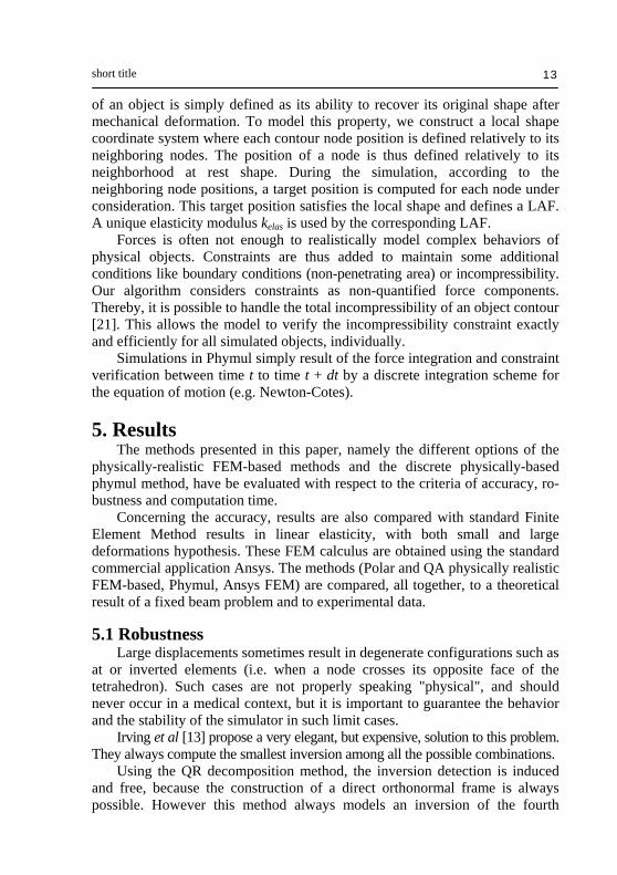
The FEM results obtained with Ansys cannot be directly compared with these values, since a single step computational cost cannot be determined. Indeed, simulation time strongly depends on the hypothesis (nonlinearity for example). 5.3 Accuracy In some fields, such as surgical planning and simulation, accuracy and precision are essential. The models have then been quantitatively evaluated, by comparison with the analytical solution of a fixed beam problem, and with the experimental results of a compression indentation of a real object. Fixed beam Following the theory of deformable beams, the deviation of a xed beam subject to gravity (fig. 8) is:

where E is the Young’s modulus and I is the moment of inertia, which depends on the geometry of the beam. The physically realistic FEM-based approaches were compared with this analytical result, modeling a beam of 40 m in length, 4 m in width and 2 m in height, with a 20 kPa Young modulus, a density of 1 and several values of Poisson’s ratios. It is known that analytically, the curve of inflection follows a polynomial of degree 4. Logarithmic scales are used to compare this degree. fig. 9 provides results obtained with three different values for Poisson's ratio. For a given Poisson's ratio value, all physically realistic FEM-based methods provide the same result. The curves being quasi-parallels, we can claim that the numerical approach follows a law of degree 4. Moreover, the simulations converge to the analytical result when Poisson’s ratio tends to zero, meeting the fact that incompressibility is not taken into account by the classical theory of beams. Truth cube New approaches to model soft tissues can be more easily experimented with phantoms than with living tissues, especially in-vivo. In a recent study,

Figure 8. Notations used for the fixed beam problem.

short title 17

Kerdok et al. [14] validated their finite element model using a cube made of silicon containing very small metal beads used to measure the effective deformations during an indentation experiment. The beads displacements, due to the indentation process, are tracked by MRI. Material properties of the silicon cube are known, i.e. a Poisson's ratio of 0:499 and a Young Modulus of 14:9 kPa. To evaluate our methods, we model this cube using a grid of 10 × 10 × 10 hexahedra, which corners positions correspond to the spheres locations. These spheres are small enough to be ignored in the simulation, which therefore assumes an isotropic behaviour of the cube. Three displacements of the cube top face are simulated (respectively 5%, 12.5% and 18.25% of compression). To test tetrahedra, we cut out each hexahedra isotropically into ten tetrahedra by superimposing the two single ways of cutting out a hexahedron into five tetrahedra (as detailled in appendix B). The material being duplicated, the Young modulus is divided by two. For the dynamic simulations, compression is applied gradually, and measurements are taken after a certain time in order to reach convergence. In term of parameter setting, a time step of 0.4 ms and 5 iterations in dynamic implicit integration are used, as well as a gravity of 9.81 and no damping. Results of the simulations are given in tables 1, 2, 3. Different methods were tested: first the pure linear geometric tensor, then using rotational invariance method with polar and QR decompositions, with or without updating the strain-displacement matrix at each time step, and with or without updating the volume term of the strain-displacement matrix. The results of a standard static linear FEM analysis (computed using the Ansys FEM software) are also presented, using the Green-Lagrange tensor in small and large deformation hypotheses (namely with and without neglecting the second order term of the tensor). The comparison criterion between simulations and measured data is based on the relative deviation:

Figure 9. Beam deviation given by the theory and by numerical results with different Poisson’s ratios.

Matthieu Nesme et al. 18

Figure 10. Simulation of the truthcube experiment.

Table 1. Results of truthcube simulations for 5% compression.

Table 2. Results of truthcube simulations for 12.5% compression.

short title 19

Table 3. Results of truthcube simulations for 18.25% compression.

linear vs non-linear. First, results given by the pure linear method and the non-linear methods are very close, which shows that the Truth cube is not enough discriminant, since elements do not undergo large enough rotations. QR B updating vs Polar B updating. As expected, the polar decomposition gives better results than QR decomposition by treating the smallest deformations. The polar decomposition give results very similar to the non-linear method, which is very interesting for interactive dynamic methods. QR B updating vs QR no B updating. With this comparison, the strain-displacement matrix updating is not very well emphasized, and do not follow the theory. That can be explained by the fact that errors accumulations of QR decomposition (discussed in section 2.4) may be compensated by errors of non-update of B, to seem to offer a good result, but it is true only in the precise case of this truthcube experiment, and is of nothing significant. This observation somewhat calls into question the use of a single "gold standard" to compare the numerical methods, a more complete set of situations is necessary. Polar B updating vs Polar no B updating. In the case of the polar decomposition the results are better when updating B, as expected. Polar V updating vs Polar no V updating. Tests on volume term updating seem to validate the fact that always using the initial volume do not decrease the precision. On the contrary, it might even improve it a little. Tetrahedron vs Hexahedron (Polar B updating). Globally, using hexahedra do not provide far more accurate results than with tetrahedra, for a computation twice longer (B updating is necessary, and there are less numerical simplifications). This result is not in agreement with the conclusions

Matthieu Nesme et al. 20

drawn by Benzley et al. [3] claiming that hexahedral elements are more accurate than tetrahedral elements in the context of FE analysis. Phymul. This method always gives a greater error than the best continuous method. However the rather small error is the price to pay for an efficient interactive computation time.

6. Conclusion Physically realistic FEM-based methods and a physically-based dicrete model were proposed for dynamic interactive simulations. Compared to theoretical and experimental data, all these methods prove to be quite relevant. Generally speaking, the results obtained with the standard FEM are slightly better, especially under a large deformation hypothesis. However, very similar values can be obtained with the polar method and the updating of the B matrix, with a far more ef cient computation time. The QR method or Phymul would be prefered if the speed criteria is the most relevant to the application, with a still excellent accuracy. These methods have now to be extensively tested with more selective data, especially when extreme boundary conditions in terms of rotations and deformations are applied, as encountered in actual biomedical interactive applications.

7. Acknowledgment We would like to thank the IMAG institute which supports this work through the MIDAS project.

Appendix A. Classical Strain-displacement matrix computation For a tetrahedron (a, b, c, d):

short title 21

The coefficients of the other shape functions are the same by a cyclic change of indices (a becomes b, b becomes c etc, and the signs also change). B. Cutting a hexahedron in five tetrahedra An hexahedron has only 2 ways of being cut out into 5 tetrahedra. For an hexahedron with vertices numbered like in fig. 11, possible cuttings are:

Figure 11. An hexahedron with indexed vertices. References 1. N. Ayache. Computational Models for the Human Body. Handbook of Numerical

Analysis (Ph. Ciarlet series editor). Elsevier, 2004. 2. D. Baraff and A. Witkin. Large steps in cloth simulation. In Proc SIGGRAPH,

1998. 3. S.E. Benzley, E. Perry, K. Merkley, and B. Clark. A comparison of all hexagonal

and all tetrahedral finite element meshes for elastic and elastoplastic analysis. In Proc. 4th International Meshing Roundtable, pages 179−191, 1995.

4. S. Cotin, H. Delingette, and N. Ayache. A hybrid elastic model allowing real-time cutting, deformations and force-feedback for surgery training and simulation. The Visual Computer, 16(8), 2000.

5. S. Cotin, H. Delingette, J.-M. Clement, V. Tassetti, J. Marescaux, and N. Ayache. Volumetric deformable models for simulation of laparoscopic surgery. In Computer Assisted Radiology, volume 1124 of International Congress Series, 1996.

6. G. Debunne, M. Desbrun M-P. Cani, and A. H. Barr. Dynamic real-time deformations using space and time adaptive sampling. In Computer Graphics Proceedings, Annual Conference Series, 2001.

7. H. Delingette. Towards realistic soft tissue modeling in medical simulation. IEEE: Special Issue on Surgery Simulation, pages 512−523, 1998.

8. H. Delingette. Towards realistic soft tissue modeling in medical simulation. In Proc of the IEEE: special issue on virtual and augmented reality in medicine, 1998.

9. O. Etzmuß, M. Keckeisen, and W. Straßer. A Fast Finite Element Solution for Cloth Modelling. Proceedings of Pacific Graphics, 2003.

10. Y.C. Fung. Biomechanics: Mechanical Properties of Living Tissues. Springer Verlag, 1993.

11. J. Garrigues. Initiation à la méthode des éléments finis. In Ecole SupÈrieure de MÈcanique de Marseille (ESM2) Courses, 2002.

Matthieu Nesme et al. 22

12. M. Hauth and W. Straßer. Corotational simulation of deformable solids. In Proc WSCG 2004, 2004.

13. G. Irving, J. Teran, and R. Fedkiw. Invertible finite elements for robust simulation of large deformation. In Proc SIGGRAPH/Eurographics Symposium on Computer Animation, 2004.

14. A. E. Kerdok, S. M. Cotin, M. P. Ottensmeyer, A. M. Galea, R. D. Howe, and S. L. Dawson. Truth cube : Establishing physical standards for real time soft tissue simulation. Medical Image Analysis, 7, 2003.

15. M. Müller, J. Dorsey, L. McMillan, R. Jagnow, and B. Cutler. Stable real-time deformations. In Proc SIGGRAPH/Eurographics Symposium on Computer Animation, 2002.

16. M. Müller and M. Gross. Interactive virtual materials. In Proceedings of Graphics Interface, 2004.

17. M. Müller, M. Teschner, and M. Gross. Physically based simulation of objects represented by surface meshes. In Proceedings of Computer Graphics International, 2004.

18. G. Picinbono, H. Delingette, and N. Ayache. Improving realism of a surgery simulator : Linear anisotropic elasticity, complex interactions and force extrapolation. Technical Report RR-4018, INRIA, 2000.

19. G. Picinbono, H. Delingette, and N. Ayache. Non-linear anisotropic elasticity for real-time surgery simulation. Graph. Models, 65(5), 2003.

20. Press, Teukolski, Vetterling, and Flannery. Numerical Recipes in C. Cambridge University Press, 1992.

21. E. Promayon, P. Baconnier, and C. Puech. Physically-based deformations constrained in displacements and volume. In Computer Graphic Forum, 1996.

22. E. Promayon, P. Baconnier, and C. Puech. Physically-based model for simulating the human trunk respiration movements. In Lecture notes in Computer Science, Springer Verlag, 1997.

23. D. Terzopoulos, J. Platt, A. Barr, and K Fleischer. Elastically deformable models. In Proc SIGGRAPH, 1987.

24. O. C. Zienkiewicz and Y. K. Cheung. The Finite Element Method in Structural and Continuum Mechanics. McGraw-Hill Publ., London, 1967.