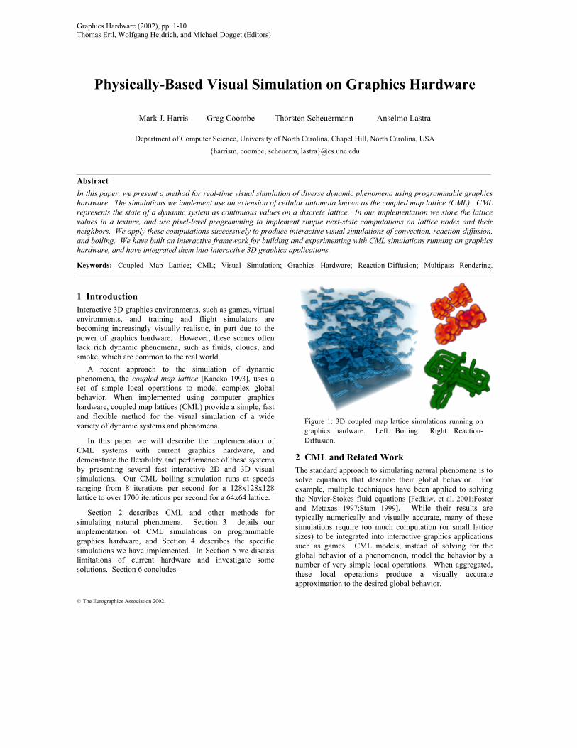
Graphics Hardware (2002), pp. 1-10 Thomas Ertl, Wolfgang Heidrich, and Michael Dogget (Editors)

© The Eurographics Association 2002.

Physically-Based Visual Simulation on Graphics Hardware

Mark J. Harris Greg Coombe Thorsten Scheuermann Anselmo Lastra

Department of Computer Science, University of North Carolina, Chapel Hill, North Carolina, USA

{harrism, coombe, scheuerm, lastra}@cs.unc.edu

Abstract In this paper, we present a method for real-time visual simulation of diverse dynamic phenomena using programmable graphics hardware. The simulations we implement use an extension of cellular automata known as the coupled map lattice (CML). CML represents the state of a dynamic system as continuous values on a discrete lattice. In our implementation we store the lattice values in a texture, and use pixel-level programming to implement simple next-state computations on lattice nodes and their neighbors. We apply these computations successively to produce interactive visual simulations of convection, reaction-diffusion, and boiling. We have built an interactive framework for building and experimenting with CML simulations running on graphics hardware, and have integrated them into interactive 3D graphics applications.

Keywords: Coupled Map Lattice; CML; Visual Simulation; Graphics Hardware; Reaction-Diffusion; Multipass Rendering.

1 Introduction Interactive 3D graphics environments, such as games, virtual environments, and training and flight simulators are becoming increasingly visually realistic, in part due to the power of graphics hardware. However, these scenes often lack rich dynamic phenomena, such as fluids, clouds, and smoke, which are common to the real world.

A recent approach to the simulation of dynamic phenomena, the coupled map lattice [Kaneko 1993], uses a set of simple local operations to model complex global behavior. When implemented using computer graphics hardware, coupled map lattices (CML) provide a simple, fast and flexible method for the visual simulation of a wide variety of dynamic systems and phenomena.

In this paper we will describe the implementation of CML systems with current graphics hardware, and demonstrate the flexibility and performance of these systems by presenting several fast interactive 2D and 3D visual simulations. Our CML boiling simulation runs at speeds ranging from 8 iterations per second for a 128x128x128 lattice to over 1700 iterations per second for a 64x64 lattice.

Section 2 describes CML and other methods for simulating natural phenomena. Section 3 details our implementation of CML simulations on programmable graphics hardware, and Section 4 describes the specific simulations we have implemented. In Section 5 we discuss limitations of current hardware and investigate some solutions. Section 6 concludes.

2 CML and Related Work The standard approach to simulating natural phenomena is to solve equations that describe their global behavior. For example, multiple techniques have been applied to solving the Navier-Stokes fluid equations [Fedkiw, et al. 2001;Foster and Metaxas 1997;Stam 1999]. While their results are typically numerically and visually accurate, many of these simulations require too much computation (or small lattice sizes) to be integrated into interactive graphics applications such as games. CML models, instead of solving for the global behavior of a phenomenon, model the behavior by a number of very simple local operations. When aggregated, these local operations produce a visually accurate approximation to the desired global behavior.

Figure 1: 3D coupled map lattice simulations running ongraphics hardware. Left: Boiling. Right: Reaction-Diffusion.

Harris, Coombe, Scheuermann, and Lastra / Simulation on Graphics Hardware

© The Eurographics Association 2002.

A coupled map lattice is a mapping of continuous dynamic state values to nodes on a lattice that interact (are ‘coupled’) with a set of other nodes in the lattice according to specified rules. Coupled map lattices were developed by Kaneko for the purpose of studying spatio-temporal dynamics and chaos [Kaneko 1993]. Since their introduction, CML techniques have been used extensively in the fields of physics and mathematics for the simulation of a variety of phenomena, including boiling [Yanagita 1992], convection [Yanagita and Kaneko 1993], cloud formation [Yanagita and Kaneko 1997], chemical reaction-diffusion [Kapral 1993], and the formation of sand ripples and dunes [Nishimori and Ouchi 1993]. CML techniques were recently introduced to the field of computer graphics for the purpose of cloud modeling and animation [Miyazaki, et al. 2001]. Lattice Boltzmann computation is a similar technique that has been used for simulating fluids, particles, and other classes of phenomena [Qian, et al. 1996].

A CML is an extension of a cellular automaton (CA) [Toffoli and Margolus 1987;von Neumann 1966;Wolfram 1984] in which the discrete state values of CA cells are replaced with continuous real values. Like CA, CML are discrete in space and time and are a versatile technique for modeling a wide variety of phenomena. Methods for animating cloud formation using cellular automata were presented in [Dobashi, et al. 2000;Nagel and Raschke 1992]. Discrete-state automata typically require very large lattices in order to simulate real phenomena, because the discrete states must be filtered in order to compute real values. By using continuous-valued state, a CML is able to represent real physical quantities at each of its nodes.

While a CML model can certainly be made both numerically and visually accurate [Kaneko 1993], our implementation on graphics hardware introduces precision constraints that make numerically accurate simulation difficult. Therefore, our goal is instead to implement visually accurate simulation models on graphics hardware, in the hope that continuing improvement in the speed and precision of graphics hardware will allow numerically accurate simulation in the near future.

The systems that have been found to be most amenable to CML implementation are multidimensional initial-value partial differential equations. These are the governing equations for a wide range of phenomena from fluid dynamics to reaction-diffusion. Based on a set of initial conditions, the simulation evolves forward in time. The only requirement is that the equation must first be explicitly discretized in space and time, which is a standard requirement for conventional numerical simulation. This flexibility means that the CML can serve as a model for a wide class of dynamic systems.

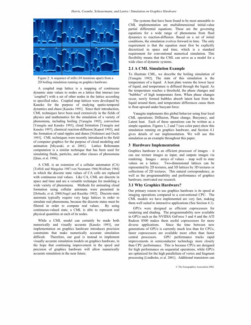
2.1 A CML Simulation Example To illustrate CML, we describe the boiling simulation of [Yanagita 1992]. The state of this simulation is the temperature of a liquid. A heat plate warms the lower layer of liquid, and temperature is diffused through the liquid. As the temperature reaches a threshold, the phase changes and “bubbles” of high temperature form. When phase changes occur, newly formed bubbles absorb latent heat from the liquid around them, and temperature differences cause them to float upward under buoyant force.

Yanagita implements this global behavior using four local CML operations; Diffusion, Phase change, Buoyancy, and Latent heat. Each of these operations can be written as a simple equation. Figures 1, 2 and 7 (see color pate) show this simulation running on graphics hardware, and Section 4.1 gives details of our implementation. We will use this simulation as an example throughout this paper.

3 Hardware Implementation Graphics hardware is an efficient processor of images – it can use texture images as input, and outputs images via rendering. Images – arrays of values – map well to state values on a lattice. Two-dimensional lattices can be represented by 2D textures, and 3D lattices by 3D textures or collections of 2D textures. This natural correspondence, as well as the programmability and performance of graphics hardware, motivated our research. 3.1 Why Graphics Hardware? Our primary reason to use graphics hardware is its speed at imaging operations compared to a conventional CPU. The CML models we have implemented are very fast, making them well suited to interactive applications (See Section 4.1).

GPUs were designed as efficient coprocessors for rendering and shading. The programmability now available in GPUs such as the NVIDIA GeForce 3 and 4 and the ATI Radeon 8500 makes them useful coprocessors for more diverse applications. Since the time between new generations of GPUs is currently much less than for CPUs, faster coprocessors are available more often than faster central processors. GPU performance tracks rapid improvements in semiconductor technology more closely than CPU performance. This is because CPUs are designed for high performance on sequential operations, while GPUs are optimized for the high parallelism of vertex and fragment processing [Lindholm, et al. 2001]. Additional transistors can

Figure 2: A sequence of stills (10 iterations apart) from a 2D boiling simulation running on graphics hardware.

Harris, Coombe, Scheuermann, and Lastra / Simulation on Graphics Hardware

© The Eurographics Association 2002.

therefore be used to greater effect in GPU architectures. In addition, programmable GPUs are inexpensive, readily available, easily upgradeable, and compatible with multiple operating systems and hardware architectures.

More importantly, interactive computer graphics applications have many components vying for processing time. Often it is difficult to efficiently perform simulation, rendering, and other computational tasks simultaneously without a drop in performance. Since our intent is visual simulation, rendering is an essential part of any solution. By moving simulation onto the GPU that renders the results of a simulation, we not only reduce computational load on the main CPU, but also avoid the substantial bus traffic required to transmit the results of a CPU simulation to the GPU for rendering. In this way, methods of dynamic simulation on the GPU provide an additional tool for load balancing in complex interactive applications.

Graphics hardware also has disadvantages. The main problems we have encountered are the difficulty of programming the GPU and the lack of high precision fragment operations and storage. These problems are related – programming difficulty is increased by the effort required to ensure that precision is conserved wherever possible.

These issues should disappear with time. Higher-level shading languages have been introduced that make hardware graphics programming easier [Peercy, et al. 2000;Proudfoot, et al. 2001]. The same or similar languages will be usable for programming simulations on graphics hardware. We believe that the precision of graphics hardware will continue to increase, and with it the full power of programmability will be realised.

3.2 General-Purpose Computation The use of computer graphics hardware for general-purpose computation has been an area of active research for many years, beginning on machines like the Ikonas [England 1978], the Pixel Machine [Potmesil and Hoffert 1989] and Pixel-Planes 5 [Rhoades, et al. 1992]. The wide deployment of GPUs in the last several years has resulted in an increase in experimental research with graphics hardware. [Trendall and Steward 2000] gives a detailed summary of the types of computation available on modern GPUs.

Within the realm of graphics applications, programmable graphics hardware has been used for procedural texturing and shading [Olano and Lastra 1998; Peercy, et al. 2000; Proudfoot, et al. 2001; Rhoades, et al. 1992]. Graphics hardware has also been used for volume visualization [Cabral, et al. 1994]. Recently, methods for using current and near-future GPUs for ray tracing computations have been described in [Carr, et al. 2002] and [Purcell, et al. 2002], respectively.

Other researchers have found ways to use graphics hardware for non-graphics applications. The use of rasterization hardware for robot motion planning is described in [Lengyel, et al. 1990]. [Hoff, et al. 1999] describes the use of z-buffer techniques for the computation of Voronoi

diagrams. The PixelFlow SIMD graphics computer [Eyles, et al. 1997] was used to crack UNIX password encryption [Kedem and Ishihara 1999], and graphics hardware has been used in the computation of artificial neural networks [Bohn 1998].

Our work uses CML to simulate dynamic phenomena that can be described by PDEs. Related to this is the visualization of flows described by PDEs, which has been implemented using graphics hardware to accelerate line integral convolution and Lagrangian-Eulerian advection [Heidrich, et al. 1999; Jobard, et al. 2001; Weiskopf, et al. 2001]. NVIDIA has demonstrated the Game of Life cellular automata running on their GPUs, as well as a 2D physically-based water simulation that operates much like our CML simulations [NVIDIA 2001a;NVIDIA 2001b].

3.3 Common Operations A detailed description of the implementation of the specific simulations that we have modeled using CML would require more space than we have in this paper, so we will instead describe a few common CML operations, followed by details of their implementation. Our goal in these descriptions is to impart a feel for the kinds of operations that can be performed using a graphics hardware implementation of a CML model. 3.3.1 Diffusion and the Laplacian The divergence of the gradient of a scalar function is called the Laplacian [Weisstein 1999]:

2 22

2 2( , ) .

T TT x y

x y

∂ ∂∇ = +

∂ ∂

The Laplacian is one of the most useful tools for working with partial differential equations. It is an isotropic measure of the second spatial derivative of a scalar function. Intuitively, it can be used to detect regions of rapid change, and for this reason it is commonly used for edge detection in image processing. The discretized form of this equation is:

2

, 1, 1, , 1 , 1 ,4i j i j i j i j i j i jT T T T T T− + − +

∇ = + + + − .

The Laplacian is used in all of the CML simulations that we have implemented. If the results of the application of a Laplacian operator at a node Ti,j are scaled and then added to the value of Ti,j itself, the result is diffusion [Weisstein 1999]:

' 2

, , ,4d

i j i j i j

cT T T= + ∇ . (1)

Here, cd is the coefficient of diffusion. Application of this diffusion operation to a lattice state will cause the state to diffuse through the lattice1. 3.3.2 Directional Forces Most dynamic simulations involve the application of force. Like all operations in a CML model, forces are applied via

1 See Appendix A for details of our diffusion implementation.

Harris, Coombe, Scheuermann, and Lastra / Simulation on Graphics Hardware

© The Eurographics Association 2002.

computations on the state of a node and its neighbors. As an example, we describe a buoyancy operator used in convection and cloud formation simulations [Miyazaki, et al. 2001;Yanagita and Kaneko 1993;Yanagita and Kaneko 1997].

This buoyancy operator uses temperature state T to compute a buoyant velocity at a node and add it to the node’s vertical velocity state, v:

, , , 1, 1,2[2 ]bc

i j i j i j i j i jv v T T T+ −

′ = + − − . (2)

Equation (2) expresses that a node is buoyed upward if its horizontal neighbors are cooler than it is, and pushed downward if they are warmer. The strength of the buoyancy is controlled via the parameter cb.

3.3.3 Computation on Neighbors Sometimes an operation requires more complex computation than the arithmetic of the simple buoyancy operation described above. The buoyancy operation of the boiling simulation described in Section 2.1 must also account for phase change, and is therefore more complicated:

, , , , 1 , 12

[ ( ) ( )],

( ) tanh[ ( )].i j i j i j i j i j

c

T T T T T

T T T

σ ρ ρ

ρ α

+ −′ = − −

= − (3)

In Equation (3), s is the buoyancy strength coefficient, and ρ(T) is an approximation of density relative to temperature, T. The hyperbolic tangent is used to simulate the rapid change of density of a substance around the phase change temperature, Tc. A change in density of a lattice node relative to its vertical neighbors causes the temperature of the node to be buoyed upward or downward. The thing to notice in this equation is that simple arithmetic will not suffice – the hyperbolic tangent function must be applied to the temperature at the neighbors above and below node (i,j). We will discuss how we can compute arbitrary functions using dependent texturing in Section 3.4.

3.4 State Representation and Storage Our goal is to maintain all state and operation of our simulations in the GPU and its associated memory. To this end, we use the frame buffer like a register array to hold transient state, and we use textures like main memory arrays

for state storage. Since the frame buffer and textures are typically limited to storage of 8-bit unsigned integers, state values must be converted to this format before being written to texture.

Texture storage can be used for both scalar and vector data. Because of the four color channels used in image generation, two-, three-, or four-dimensional vectors can be stored in each texel of an RGBA texture. If scalar data are needed, it is often advantageous to store more than one scalar state in a single texture by using different color channels. In our CML implementation of the Gray-Scott reaction-diffusion system, for example, we store the concentrations of both reactants in the same texture. This is not only efficient in storage but also in computation since operations that act equivalently on both concentrations can be performed in parallel.

Physical simulation also requires the use of signed values. Most texture storage, however, uses unsigned fixed-point values. Although fragment-level programmability available in current GPUs uses signed arithmetic internally, the unsigned data stored in the textures must be biased and scaled before and after processing [NVIDIA 2002].

3.5 Implementing CML Operations An iteration of a CML simulation consists of successive application of simple operations on the lattice. These operations consist of three steps: setup the graphics hardware rendering state, render a single quadrilateral fit to the view port, and store the rendered results into a texture. We refer to each of these setup-render-copy operations as a single pass. In practice, due to limited GPU resources (number of texture units, number of register combiners, etc.), a CML operation may span multiple passes.

The setup portion of a pass simply sets the state of the hardware to correctly perform the rest of the pass. To be sure that the correct lattice nodes are sampled during the pass, texels in the input textures must map directly to pixels in the output of the graphics pipeline. To ensure that this is true, we set the view port to the resolution of the lattice, and the view frustum to an orthographic view fit to the lattice so that there is a one-to-one mapping between pixels in the rendering buffer and texels in the texture to be updated.

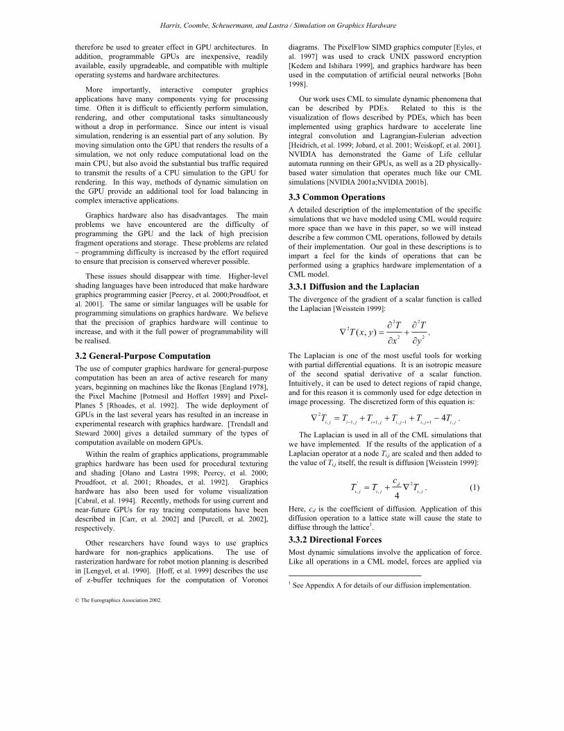
The render-copy portion of each pass performs 4 suboperations: Neighbor Sampling, Computation on Neighbors, New State Computation, and State Update. Figure 3 illustrates the mapping of the suboperations to graphics hardware. Neighbor sampling and Computation on Neighbors are performed by the programmable texture mapping hardware. New State Computation performs arithmetic on the results of the previous suboperations using programmable texture blending. Finally, State Update feeds the results of one pass to the next by rendering or copying the texture blending results to a texture.

Neighbor Sampling: Since state is stored in textures, neighbor sampling is performed by offsetting texture coordinates toward the neighbors of the texel being updated.

Figure 3: Components of a CML operation map to graphics hardware pipeline components.

Harris, Coombe, Scheuermann, and Lastra / Simulation on Graphics Hardware

© The Eurographics Association 2002.

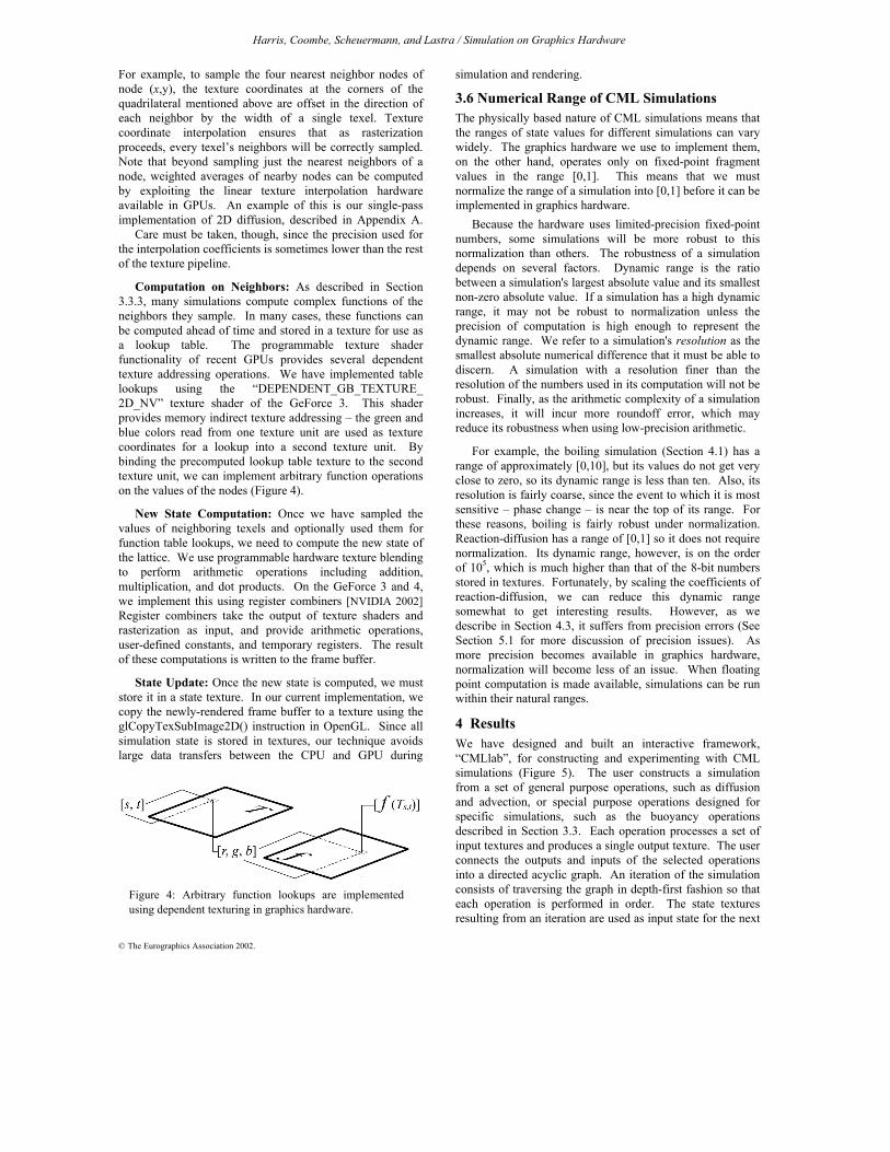
For example, to sample the four nearest neighbor nodes of node (x,y), the texture coordinates at the corners of the quadrilateral mentioned above are offset in the direction of each neighbor by the width of a single texel. Texture coordinate interpolation ensures that as rasterization proceeds, every texel’s neighbors will be correctly sampled. Note that beyond sampling just the nearest neighbors of a node, weighted averages of nearby nodes can be computed by exploiting the linear texture interpolation hardware available in GPUs. An example of this is our single-pass implementation of 2D diffusion, described in Appendix A.

Care must be taken, though, since the precision used for the interpolation coefficients is sometimes lower than the rest of the texture pipeline.

Computation on Neighbors: As described in Section 3.3.3, many simulations compute complex functions of the neighbors they sample. In many cases, these functions can be computed ahead of time and stored in a texture for use as a lookup table. The programmable texture shader functionality of recent GPUs provides several dependent texture addressing operations. We have implemented table lookups using the “DEPENDENT_GB_TEXTURE_ 2D_NV” texture shader of the GeForce 3. This shader provides memory indirect texture addressing – the green and blue colors read from one texture unit are used as texture coordinates for a lookup into a second texture unit. By binding the precomputed lookup table texture to the second texture unit, we can implement arbitrary function operations on the values of the nodes (Figure 4).

New State Computation: Once we have sampled the values of neighboring texels and optionally used them for function table lookups, we need to compute the new state of the lattice. We use programmable hardware texture blending to perform arithmetic operations including addition, multiplication, and dot products. On the GeForce 3 and 4, we implement this using register combiners [NVIDIA 2002] Register combiners take the output of texture shaders and rasterization as input, and provide arithmetic operations, user-defined constants, and temporary registers. The result of these computations is written to the frame buffer.

State Update: Once the new state is computed, we must store it in a state texture. In our current implementation, we copy the newly-rendered frame buffer to a texture using the glCopyTexSubImage2D() instruction in OpenGL. Since all simulation state is stored in textures, our technique avoids large data transfers between the CPU and GPU during

simulation and rendering.

3.6 Numerical Range of CML Simulations The physically based nature of CML simulations means that the ranges of state values for different simulations can vary widely. The graphics hardware we use to implement them, on the other hand, operates only on fixed-point fragment values in the range [0,1]. This means that we must normalize the range of a simulation into [0,1] before it can be implemented in graphics hardware.

Because the hardware uses limited-precision fixed-point numbers, some simulations will be more robust to this normalization than others. The robustness of a simulation depends on several factors. Dynamic range is the ratio between a simulation's largest absolute value and its smallest non-zero absolute value. If a simulation has a high dynamic range, it may not be robust to normalization unless the precision of computation is high enough to represent the dynamic range. We refer to a simulation's resolution as the smallest absolute numerical difference that it must be able to discern. A simulation with a resolution finer than the resolution of the numbers used in its computation will not be robust. Finally, as the arithmetic complexity of a simulation increases, it will incur more roundoff error, which may reduce its robustness when using low-precision arithmetic.

For example, the boiling simulation (Section 4.1) has a range of approximately [0,10], but its values do not get very close to zero, so its dynamic range is less than ten. Also, its resolution is fairly coarse, since the event to which it is most sensitive – phase change – is near the top of its range. For these reasons, boiling is fairly robust under normalization. Reaction-diffusion has a range of [0,1] so it does not require normalization. Its dynamic range, however, is on the order of 105, which is much higher than that of the 8-bit numbers stored in textures. Fortunately, by scaling the coefficients of reaction-diffusion, we can reduce this dynamic range somewhat to get interesting results. However, as we describe in Section 4.3, it suffers from precision errors (See Section 5.1 for more discussion of precision issues). As more precision becomes available in graphics hardware, normalization will become less of an issue. When floating point computation is made available, simulations can be run within their natural ranges.

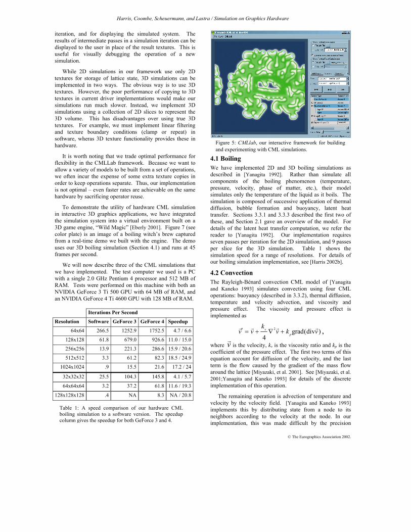
4 Results We have designed and built an interactive framework, “CMLlab”, for constructing and experimenting with CML simulations (Figure 5). The user constructs a simulation from a set of general purpose operations, such as diffusion and advection, or special purpose operations designed for specific simulations, such as the buoyancy operations described in Section 3.3. Each operation processes a set of input textures and produces a single output texture. The user connects the outputs and inputs of the selected operations into a directed acyclic graph. An iteration of the simulation consists of traversing the graph in depth-first fashion so that each operation is performed in order. The state textures resulting from an iteration are used as input state for the next

Figure 4: Arbitrary function lookups are implementedusing dependent texturing in graphics hardware.

Harris, Coombe, Scheuermann, and Lastra / Simulation on Graphics Hardware

© The Eurographics Association 2002.

iteration, and for displaying the simulated system. The results of intermediate passes in a simulation iteration can be displayed to the user in place of the result textures. This is useful for visually debugging the operation of a new simulation.

While 2D simulations in our framework use only 2D textures for storage of lattice state, 3D simulations can be implemented in two ways. The obvious way is to use 3D textures. However, the poor performance of copying to 3D textures in current driver implementations would make our simulations run much slower. Instead, we implement 3D simulations using a collection of 2D slices to represent the 3D volume. This has disadvantages over using true 3D textures. For example, we must implement linear filtering and texture boundary conditions (clamp or repeat) in software, wheras 3D texture functionality provides these in hardware.

It is worth noting that we trade optimal performance for flexibility in the CMLLab framework. Because we want to allow a variety of models to be built from a set of operations, we often incur the expense of some extra texture copies in order to keep operations separate. Thus, our implementation is not optimal – even faster rates are achievable on the same hardware by sacrificing operator reuse.

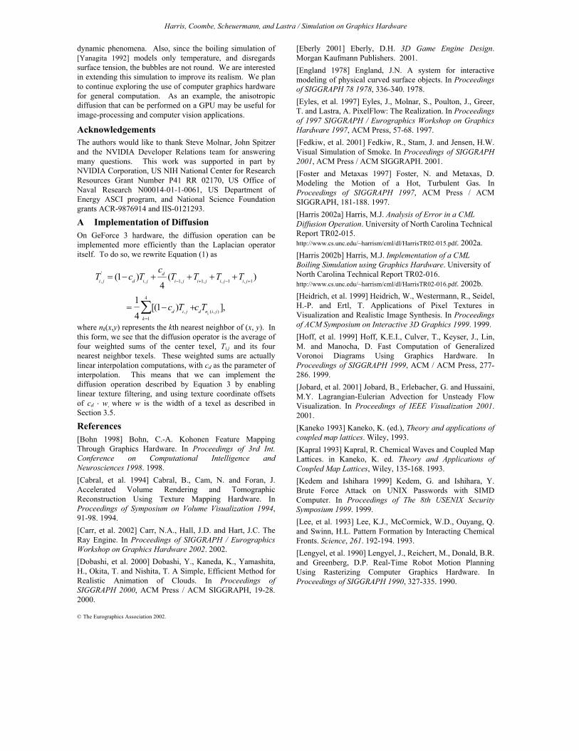
To demonstrate the utility of hardware CML simulation in interactive 3D graphics applications, we have integrated the simulation system into a virtual environment built on a 3D game engine, “Wild Magic” [Eberly 2001]. Figure 7 (see color plate) is an image of a boiling witch’s brew captured from a real-time demo we built with the engine. The demo uses our 3D boiling simulation (Section 4.1) and runs at 45 frames per second.

We will now describe three of the CML simulations that we have implemented. The test computer we used is a PC with a single 2.0 GHz Pentium 4 processor and 512 MB of RAM. Tests were performed on this machine with both an NVIDIA GeForce 3 Ti 500 GPU with 64 MB of RAM, and an NVIDIA GeForce 4 Ti 4600 GPU with 128 MB of RAM.

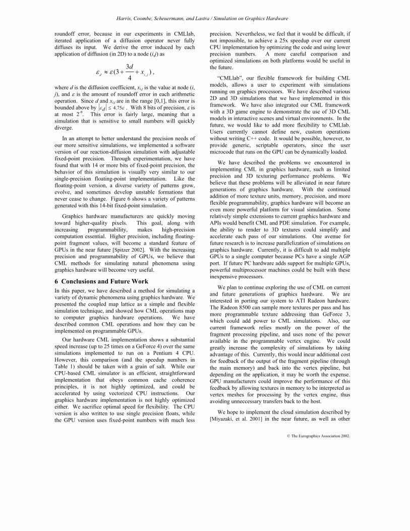
4.1 Boiling We have implemented 2D and 3D boiling simulations as described in [Yanagita 1992]. Rather than simulate all components of the boiling phenomenon (temperature, pressure, velocity, phase of matter, etc.), their model simulates only the temperature of the liquid as it boils. The simulation is composed of successive application of thermal diffusion, bubble formation and buoyancy, latent heat transfer. Sections 3.3.1 and 3.3.3 described the first two of these, and Section 2.1 gave an overview of the model. For details of the latent heat transfer computation, we refer the reader to [Yanagita 1992]. Our implementation requires seven passes per iteration for the 2D simulation, and 9 passes per slice for the 3D simulation. Table 1 shows the simulation speed for a range of resolutions. For details of our boiling simulation implementation, see [Harris 2002b].

4.2 Convection The Rayleigh-Bénard convection CML model of [Yanagita and Kaneko 1993] simulates convection using four CML operations: buoyancy (described in 3.3.2), thermal diffusion, temperature and velocity advection, and viscosity and pressure effect. The viscosity and pressure effect is implemented as

2 grad(div )4

vp

kv v v k v′ = + ∇ + ,

where v is the velocity, kv is the viscosity ratio and kp is the coefficient of the pressure effect. The first two terms of this equation account for diffusion of the velocity, and the last term is the flow caused by the gradient of the mass flow around the lattice [Miyazaki, et al. 2001]. See [Miyazaki, et al. 2001;Yanagita and Kaneko 1993] for details of the discrete implementation of this operation.

The remaining operation is advection of temperature and velocity by the velocity field. [Yanagita and Kaneko 1993] implements this by distributing state from a node to its neighbors according to the velocity at the node. In our implementation, this was made difficult by the precision

Iterations Per Second

Resolution Software GeForce 3 GeForce 4 Speedup

64x64 266.5 1252.9 1752.5 4.7 / 6.6

128x128 61.8 679.0 926.6 11.0 / 15.0

256x256 13.9 221.3 286.6 15.9 / 20.6

512x512 3.3 61.2 82.3 18.5 / 24.9

1024x1024 .9 15.5 21.6 17.2 / 24

32x32x32 25.5 104.3 145.8 4.1 / 5.7

64x64x64 3.2 37.2 61.8 11.6 / 19.3

128x128x128 .4 NA 8.3 NA / 20.8

Table 1: A speed comparison of our hardware CMLboiling simulation to a software version. The speedupcolumn gives the speedup for both GeForce 3 and 4.

Figure 5: CMLlab, our interactive framework for buildingand experimenting with CML simulations.

Harris, Coombe, Scheuermann, and Lastra / Simulation on Graphics Hardware

© The Eurographics Association 2002.

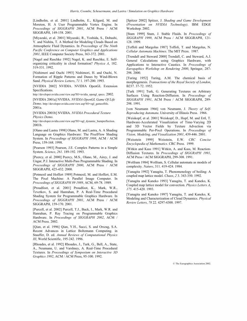
limitations of the hardware, so we used a texture shader-based advection operation instead. This operation advects state stored in a texture using the GL_OFFSET_TEXTURE_ 2D_NV dependent texture addressing mode of the GeForce 3 and 4. A description of this method can be found in [Weiskopf, et al. 2001]. Our 2D convection implementation (Figure 8 in the color plate section) requires 10 passes per iteration. We have not implemented a 3D convection simulation because GeForce 3 and 4 do not have a 3D equivalent of the offset texture operation.

Due to the precision limitations of the graphics hardware, our implementation of convection did not behave exactly as described by [Yanagita and Kaneko 1993]. We do observe the formation of convective rolls, but the motion of both the temperature and velocity fields is quite turbulent. We believe that this is a result of low-precision arithmetic.

4.3 Reaction-Diffusion Reaction-Diffusion processes were proposed by [Turing 1952] and introduced to computer graphics by [Turk 1991;Witkin and Kass 1991]. They are a well-studied model for the interaction of chemical reactants, and are interesting due to their complex and often chaotic behavior. The patterns that emerge are reminiscent of patterns occurring in nature [Lee, et al. 1993]. We implemented the Gray-Scott model, as described in [Pearson 1993]. This is a two-chemical system defined by the initial value partial differential equations:

2 2

2 2

(1 )

( ) ,

u

v

UD U UV F U

tV

D V UV F k Vt

∂= ∇ − + −

∂

∂= ∇ + − +

∂

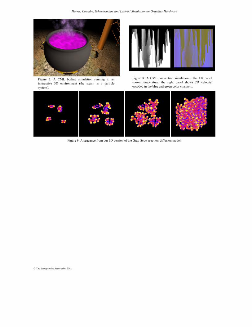
where F, k, Du, and Dv. are parameters given in [Pearson 1993]. We have implemented 2D and 3D versions of this process, as shown in Figure 5 (2D), and Figures 1 and 9 (3D, on color plate). We found reaction-diffusion relatively simple to implement in our framework because we were able to reuse our existing diffusion operator. In 2D this

simulation requires two passes per iteration, and in 3D it requires three passes per slice. A 256x256 lattice runs at 400 iterations per second in our interactive framework, and a 128x128x32 lattice runs at 60 iterations per second.

The low precision of the GeForce 3 and 4 reduces the variety of patterns that our implementation of the Gray-Scott model produces. We have seen a variety of results, but much less diversity than produced by a floating point implementation. As with convection, this appears to be caused by the effects of low-precision arithmetic.

5 Hardware Limitations While current GPUs make a good platform for CML simulation, they are not without problems. Some of these problems are performance problems of the current implementation, and may not be issues in the near future. NVIDIA has shown in the past that slow performance can often be alleviated via optimization of the software drivers that accompany the GPU. Other limitations are more fundamental.

Most of the implementation limitations that we encountered were limitations that affected performance. We have found glCopyTexSubImage3D(), which copies the frame buffer to a slice of a 3D texture, to be much slower (up to three orders of magnitude) than glCopyTexSubImage2D() for the same amount of data. This prevented us from using 3D textures in our implementation. Once this problem is alleviated, we expect a 3D texture implementation to be faster and easier to implement, since it will remove the need to bind multiple textures to sample neighbors in the third dimension. Also, 3D textures provide hardware linear interpolation and boundary conditions (periodic or fixed) in all three dimensions. With our slice-based implementation, we must interpolate and handle boundary conditions in the third dimension in software.

The ability to render to texture will also provide a speed improvement, as we estimate that in a complex 3D simulation, much of the processing time is spent copying rendered data from the frame buffer to textures (typically one copy per pass). When using 3D textures, we will need the ability to render to a slice of a 3D texture.

5.1 Precision The hardware limitation that causes the most problems to

our implementation is precision. The register combiners in the GeForce 3 and 4 perform arithmetic using nine-bit signed fixed-point values. Without floating point, the programmer must scale and bias values to maintain them in ranges that maximize precision. This is not only difficult, it is subject to arithmetic error. Some simulations (such as boiling) handle this error well, and behave as predicted by a floating point implementation. Others, such as our reaction-diffusion implementation, are more sensitive to precision errors.

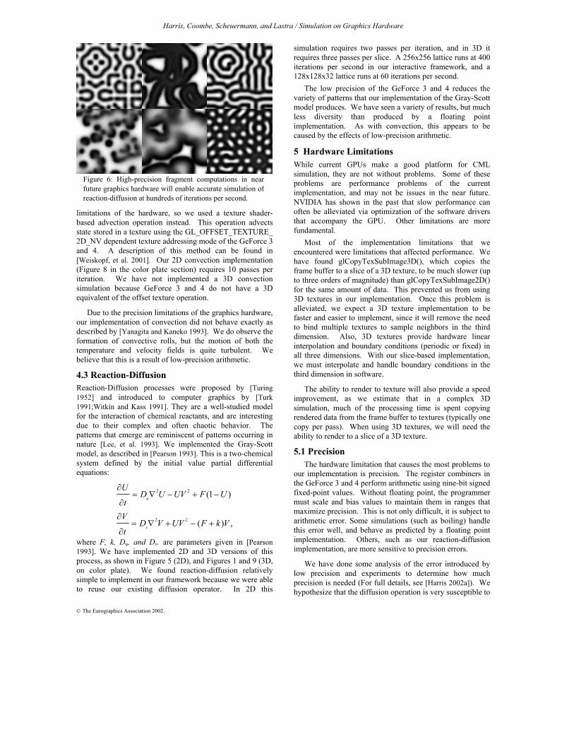
We have done some analysis of the error introduced by low precision and experiments to determine how much precision is needed (For full details, see [Harris 2002a]). We hypothesize that the diffusion operation is very susceptible to

Figure 6: High-precision fragment computations in nearfuture graphics hardware will enable accurate simulation ofreaction-diffusion at hundreds of iterations per second.

Harris, Coombe, Scheuermann, and Lastra / Simulation on Graphics Hardware

© The Eurographics Association 2002.

roundoff error, because in our experiments in CMLlab, iterated application of a diffusion operator never fully diffuses its input. We derive the error induced by each application of diffusion (in 2D) to a node (i,j) as

,

3(3 )

4d i j

dxε ε≈ + + ,

where d is the diffusion coefficient, xi,j is the value at node (i, j), and ε is the amount of roundoff error in each arithmetic operation. Since d and xi,j are in the range [0,1], this error is bounded above by 4.75dε ε≤ . With 8 bits of precision, ε is at most 2-9. This error is fairly large, meaning that a simulation that is sensitive to small numbers will quickly diverge.

In an attempt to better understand the precision needs of our more sensitive simulations, we implemented a software version of our reaction-diffusion simulation with adjustable fixed-point precision. Through experimentation, we have found that with 14 or more bits of fixed-point precision, the behavior of this simulation is visually very similar to our single-precision floating-point implementation. Like the floating-point version, a diverse variety of patterns grow, evolve, and sometimes develop unstable formations that never cease to change. Figure 6 shows a variety of patterns generated with this 14-bit fixed-point simulation.

Graphics hardware manufacturers are quickly moving toward higher-quality pixels. This goal, along with increasing programmability, makes high-precision computation essential. Higher precision, including floating-point fragment values, will become a standard feature of GPUs in the near future [Spitzer 2002]. With the increasing precision and programmability of GPUs, we believe that CML methods for simulating natural phenomena using graphics hardware will become very useful.

6 Conclusions and Future Work In this paper, we have described a method for simulating a variety of dynamic phenomena using graphics hardware. We presented the coupled map lattice as a simple and flexible simulation technique, and showed how CML operations map to computer graphics hardware operations. We have described common CML operations and how they can be implemented on programmable GPUs.

Our hardware CML implementation shows a substantial speed increase (up to 25 times on a GeForce 4) over the same simulations implemented to run on a Pentium 4 CPU. However, this comparison (and the speedup numbers in Table 1) should be taken with a grain of salt. While our CPU-based CML simulator is an efficient, straightforward implementation that obeys common cache coherence principles, it is not highly optimized, and could be accelerated by using vectorized CPU instructions. Our graphics hardware implementation is not highly optimized either. We sacrifice optimal speed for flexibility. The CPU version is also written to use single precision floats, while the GPU version uses fixed-point numbers with much less

precision. Nevertheless, we feel that it would be difficult, if not impossible, to achieve a 25x speedup over our current CPU implementation by optimizing the code and using lower precision numbers. A more careful comparison and optimized simulations on both platforms would be useful in the future.

“CMLlab”, our flexible framework for building CML models, allows a user to experiment with simulations running on graphics processors. We have described various 2D and 3D simulations that we have implemented in this framework. We have also integrated our CML framework with a 3D game engine to demonstrate the use of 3D CML models in interactive scenes and virtual environments. In the future, we would like to add more flexibility to CMLlab. Users currently cannot define new, custom operations without writing C++ code. It would be possible, however, to provide generic, scriptable operators, since the user microcode that runs on the GPU can be dynamically loaded.

We have described the problems we encountered in implementing CML in graphics hardware, such as limited precision and 3D texturing performance problems. We believe that these problems will be alleviated in near future generations of graphics hardware. With the continued addition of more texture units, memory, precision, and more flexible programmability, graphics hardware will become an even more powerful platform for visual simulation. Some relatively simple extensions to current graphics hardware and APIs would benefit CML and PDE simulation. For example, the ability to render to 3D textures could simplify and accelerate each pass of our simulations. One avenue for future research is to increase parallelization of simulations on graphics hardware. Currently, it is difficult to add multiple GPUs to a single computer because PCs have a single AGP port. If future PC hardware adds support for multiple GPUs, powerful multiprocessor machines could be built with these inexpensive processors.

We plan to continue exploring the use of CML on current and future generations of graphics hardware. We are interested in porting our system to ATI Radeon hardware. The Radeon 8500 can sample more textures per pass and has more programmable texture addressing than GeForce 3, which could add power to CML simulations. Also, our current framework relies mostly on the power of the fragment processing pipeline, and uses none of the power available in the programmable vertex engine. We could greatly increase the complexity of simulations by taking advantage of this. Currently, this would incur additional cost for feedback of the output of the fragment pipeline (through the main memory) and back into the vertex pipeline, but depending on the application, it may be worth the expense. GPU manufacturers could improve the performance of this feedback by allowing textures in memory to be interpreted as vertex meshes for processing by the vertex engine, thus avoiding unneccessary transfers back to the host.

We hope to implement the cloud simulation described by [Miyazaki, et al. 2001] in the near future, as well as other

Harris, Coombe, Scheuermann, and Lastra / Simulation on Graphics Hardware

© The Eurographics Association 2002.

dynamic phenomena. Also, since the boiling simulation of [Yanagita 1992] models only temperature, and disregards surface tension, the bubbles are not round. We are interested in extending this simulation to improve its realism. We plan to continue exploring the use of computer graphics hardware for general computation. As an example, the anisotropic diffusion that can be performed on a GPU may be useful for image-processing and computer vision applications.

Acknowledgements The authors would like to thank Steve Molnar, John Spitzer and the NVIDIA Developer Relations team for answering many questions. This work was supported in part by NVIDIA Corporation, US NIH National Center for Research Resources Grant Number P41 RR 02170, US Office of Naval Research N00014-01-1-0061, US Department of Energy ASCI program, and National Science Foundation grants ACR-9876914 and IIS-0121293.

A Implementation of Diffusion On GeForce 3 hardware, the diffusion operation can be implemented more efficiently than the Laplacian operator itself. To do so, we rewrite Equation (1) as

'

, , 1, 1, , 1 , 1

4

, ( , )1

(1 ) ( )4

1[(1 ) ],

4 k

di j d i j i j i j i j i j

d i j d n i jk

cT c T T T T T

c T c T

− + − +

=

= − + + + +

= − +∑

where nk(x,y) represents the kth nearest neighbor of (x, y). In this form, we see that the diffusion operator is the average of four weighted sums of the center texel, Ti,j and its four nearest neighbor texels. These weighted sums are actually linear interpolation computations, with cd as the parameter of interpolation. This means that we can implement the diffusion operation described by Equation 3 by enabling linear texture filtering, and using texture coordinate offsets of cd ÿ w, where w is the width of a texel as described in Section 3.5.

References [Bohn 1998] Bohn, C.-A. Kohonen Feature Mapping Through Graphics Hardware. In Proceedings of 3rd Int. Conference on Computational Intelligence and Neurosciences 1998. 1998. [Cabral, et al. 1994] Cabral, B., Cam, N. and Foran, J. Accelerated Volume Rendering and Tomographic Reconstruction Using Texture Mapping Hardware. In Proceedings of Symposium on Volume Visualization 1994, 91-98. 1994. [Carr, et al. 2002] Carr, N.A., Hall, J.D. and Hart, J.C. The Ray Engine. In Proceedings of SIGGRAPH / Eurographics Workshop on Graphics Hardware 2002. 2002. [Dobashi, et al. 2000] Dobashi, Y., Kaneda, K., Yamashita, H., Okita, T. and Nishita, T. A Simple, Efficient Method for Realistic Animation of Clouds. In Proceedings of SIGGRAPH 2000, ACM Press / ACM SIGGRAPH, 19-28. 2000.

[Eberly 2001] Eberly, D.H. 3D Game Engine Design. Morgan Kaufmann Publishers. 2001. [England 1978] England, J.N. A system for interactive modeling of physical curved surface objects. In Proceedings of SIGGRAPH 78 1978, 336-340. 1978. [Eyles, et al. 1997] Eyles, J., Molnar, S., Poulton, J., Greer, T. and Lastra, A. PixelFlow: The Realization. In Proceedings of 1997 SIGGRAPH / Eurographics Workshop on Graphics Hardware 1997, ACM Press, 57-68. 1997. [Fedkiw, et al. 2001] Fedkiw, R., Stam, J. and Jensen, H.W. Visual Simulation of Smoke. In Proceedings of SIGGRAPH 2001, ACM Press / ACM SIGGRAPH. 2001. [Foster and Metaxas 1997] Foster, N. and Metaxas, D. Modeling the Motion of a Hot, Turbulent Gas. In Proceedings of SIGGRAPH 1997, ACM Press / ACM SIGGRAPH, 181-188. 1997. [Harris 2002a] Harris, M.J. Analysis of Error in a CML Diffusion Operation. University of North Carolina Technical Report TR02-015. http://www.cs.unc.edu/~harrism/cml/dl/HarrisTR02-015.pdf. 2002a. [Harris 2002b] Harris, M.J. Implementation of a CML Boiling Simulation using Graphics Hardware. University of North Carolina Technical Report TR02-016. http://www.cs.unc.edu/~harrism/cml/dl/HarrisTR02-016.pdf. 2002b. [Heidrich, et al. 1999] Heidrich, W., Westermann, R., Seidel, H.-P. and Ertl, T. Applications of Pixel Textures in Visualization and Realistic Image Synthesis. In Proceedings of ACM Symposium on Interactive 3D Graphics 1999. 1999. [Hoff, et al. 1999] Hoff, K.E.I., Culver, T., Keyser, J., Lin, M. and Manocha, D. Fast Computation of Generalized Voronoi Diagrams Using Graphics Hardware. In Proceedings of SIGGRAPH 1999, ACM / ACM Press, 277-286. 1999. [Jobard, et al. 2001] Jobard, B., Erlebacher, G. and Hussaini, M.Y. Lagrangian-Eulerian Advection for Unsteady Flow Visualization. In Proceedings of IEEE Visualization 2001. 2001. [Kaneko 1993] Kaneko, K. (ed.), Theory and applications of coupled map lattices. Wiley, 1993. [Kapral 1993] Kapral, R. Chemical Waves and Coupled Map Lattices. in Kaneko, K. ed. Theory and Applications of Coupled Map Lattices, Wiley, 135-168. 1993. [Kedem and Ishihara 1999] Kedem, G. and Ishihara, Y. Brute Force Attack on UNIX Passwords with SIMD Computer. In Proceedings of The 8th USENIX Security Symposium 1999. 1999. [Lee, et al. 1993] Lee, K.J., McCormick, W.D., Ouyang, Q. and Swinn, H.L. Pattern Formation by Interacting Chemical Fronts. Science, 261. 192-194. 1993. [Lengyel, et al. 1990] Lengyel, J., Reichert, M., Donald, B.R. and Greenberg, D.P. Real-Time Robot Motion Planning Using Rasterizing Computer Graphics Hardware. In Proceedings of SIGGRAPH 1990, 327-335. 1990.

Harris, Coombe, Scheuermann, and Lastra / Simulation on Graphics Hardware

© The Eurographics Association 2002.

[Lindholm, et al. 2001] Lindholm, E., Kilgard, M. and Moreton, H. A User Programmable Vertex Engine. In Proceedings of SIGGRAPH 2001, ACM Press / ACM SIGGRAPH, 149-158. 2001. [Miyazaki, et al. 2001] Miyazaki, R., Yoshida, S., Dobashi, Y. and Nishita, T. A Method for Modeling Clouds Based on Atmospheric Fluid Dynamics. In Proceedings of The Ninth Pacific Conference on Computer Graphics and Applications 2001, IEEE Computer Society Press, 363-372. 2001. [Nagel and Raschke 1992] Nagel, K. and Raschke, E. Self-organizing criticality in cloud formation? Physica A, 182. 519-531. 1992. [Nishimori and Ouchi 1993] Nishimori, H. and Ouchi, N. Formation of Ripple Patterns and Dunes by Wind-Blown Sand. Physical Review Letters, 71 1. 197-200. 1993. [NVIDIA 2002] NVIDIA. NVIDIA OpenGL Extension Specifications. http://developer.nvidia.com/view.asp?IO=nvidia_opengl_specs. 2002. [NVIDIA 2001a] NVIDIA. NVIDIA OpenGL Game Of Life Demo. http://developer.nvidia.com/view.asp?IO=ogl_gameoflife. 2001a. [NVIDIA 2001b] NVIDIA. NVIDIA Procedural Texture Physics Demo. http://developer.nvidia.com/view.asp?IO=ogl_dynamic_bumpreflection. 2001b. [Olano and Lastra 1998] Olano, M. and Lastra, A. A Shading Language on Graphics Hardware: The PixelFlow Shading System. In Proceedings of SIGGRAPH 1998, ACM / ACM Press, 159-168. 1998. [Pearson 1993] Pearson, J.E. Complex Patterns in a Simple System. Science, 261. 189-192. 1993. [Peercy, et al. 2000] Peercy, M.S., Olano, M., Airey, J. and Ungar, P.J. Interactive Multi-Pass Programmable Shading. In Proceedings of SIGGRAPH 2000, ACM Press / ACM SIGGRAPH, 425-432. 2000. [Potmesil and Hoffert 1989] Potmesil, M. and Hoffert, E.M. The Pixel Machine: A Parallel Image Computer. In Proceedings of SIGGRAPH 89 1989, ACM, 69-78. 1989. [Proudfoot, et al. 2001] Proudfoot, K., Mark, W.R., Tzvetkov, S. and Hanrahan, P. A Real-Time Procedural Shading System for Programmable Graphics Hardware. In Proceedings of SIGGRAPH 2001, ACM Press / ACM SIGGRAPH, 159-170. 2001. [Purcell, et al. 2002] Purcell, T.J., Buck, I., Mark, W.R. and Hanrahan, P. Ray Tracing on Programmable Graphics Hardware. In Proceedings of SIGGRAPH 2002, ACM / ACM Press. 2002. [Qian, et al. 1996] Qian, Y.H., Succi, S. and Orszag, S.A. Recent Advances in Lattice Boltzmann Computing. in Stauffer, D. ed. Annual Reviews of Computational Physics III, World Scientific, 195-242. 1996. [Rhoades, et al. 1992] Rhoades, J., Turk, G., Bell, A., State, A., Neumann, U. and Varshney, A. Real-Time Procedural Textures. In Proceedings of Symposium on Interactive 3D Graphics 1992, ACM / ACM Press, 95-100. 1992.

[Spitzer 2002] Spitzer, J. Shading and Game Development (Presentation on NVIDIA Technology). IBM EDGE Workshop. 2002. [Stam 1999] Stam, J. Stable Fluids. In Proceedings of SIGGRAPH 1999, ACM Press / ACM SIGGRAPH, 121-128. 1999. [Toffoli and Margolus 1987] Toffoli, T. and Margolus, N. Cellular Automata Machines. The MIT Press. 1987. [Trendall and Steward 2000] Trendall, C. and Steward, A.J. General Calculations using Graphics Hardware, with Applications to Interactive Caustics. In Proceedings of Eurogaphics Workshop on Rendering 2000, Springer, 287-298. 2000. [Turing 1952] Turing, A.M. The chemical basis of morphogenesis. Transactions of the Royal Society of London, B237. 37-72. 1952. [Turk 1991] Turk, G. Generating Textures on Arbitrary Surfaces Using Reaction-Diffusion. In Proceedings of SIGGRAPH 1991, ACM Press / ACM SIGGRAPH, 289-298. 1991. [von Neumann 1966] von Neumann, J. Theory of Self-Reproducing Automata. University of Illinois Press. 1966. [Weiskopf, et al. 2001] Weiskopf, D., Hopf, M. and Ertl, T. Hardware-Accelerated Visualization of Time-Varying 2D and 3D Vector Fields by Texture Advection via Programmable Per-Pixel Operations. In Proceedings of Vision, Modeling, and Visualization 2001, 439-446. 2001. [Weisstein 1999] Weisstein, E.W. CRC Concise Encyclopedia of Mathematics. CRC Press. 1999. [Witkin and Kass 1991] Witkin, A. and Kass, M. Reaction-Diffusion Textures. In Proceedings of SIGGRAPH 1991, ACM Press / ACM SIGGRAPH, 299-308. 1991. [Wolfram 1984] Wolfram, S. Cellular automata as models of complexity. Nature, 311. 419-424. 1984. [Yanagita 1992] Yanagita, T. Phenomenology of boiling: A coupled map lattice model. Chaos, 2 3. 343-350. 1992. [Yanagita and Kaneko 1993] Yanagita, T. and Kaneko, K. Coupled map lattice model for convection. Physics Letters A, 175. 415-420. 1993. [Yanagita and Kaneko 1997] Yanagita, T. and Kaneko, K. Modeling and Characterization of Cloud Dynamics. Physical Review Letters, 78 22. 4297-4300. 1997.

Harris, Coombe, Scheuermann, and Lastra / Simulation on Graphics Hardware

© The Eurographics Association 2002.

Figure 7: A CML boiling simulation running in aninteractive 3D environment (the steam is a particlesystem).

Figure 9: A sequence from our 3D version of the Gray-Scott reaction-diffusion model.

Figure 8: A CML convection simulation. The left panelshows temperature; the right panel shows 2D velocityencoded in the blue and green color channels.