Lauri Viitanen

Physically Based Terrain Generation Procedural Heightmap Generation Using Plate Tectonics

Helsinki Metropolia University of Applied Sciences Bachelor of Engineering Information Technology Thesis 30.3.2012

Abstract

Author Title Number of Pages Date

Lauri Viitanen Physically Based Terrain Generation 63 pages + 1 appendix 30 March 2012

Degree Bachelor of Engineering

Degree Programme Information Technology

Specialization option Software engineering

Instructors

Miikka Mäki-Uuro, Senior Lecturer Juha Kopu, Senior Lecturer

This thesis explores the usefulness of the theory of plate tectonics in procedural terrain generation. The objective is to produce a model that's based on plate tectonics and use it to investigate the benefits and drawbacks of simulating the movement and dynamics of tectonic plates. The study briefly reviews the procedural methods that are currently used in the game and film industries to produce artificial terrain and discusses their strengths and weaknesses. Utilization of plate tectonics in the generation of artificial heightmaps is suggested and the theory behind it is covered in appropriate detail. The thesis examines some related previ-ous works before introducing a new computer implementation of a terrain generator that is based on plate tectonics. The resulting implementation is able to produce far more realistic heightmaps more au-tonomously than what is possible with most conventional methods. Coupled with the rela-tively low level of technical competency required to implement the terrain generator it becomes evident that the simulation of plate tectonics is a plausible method for procedural terrain generation for hobbyists and professionals alike.

Keywords procedural, terrain, heightmap, generation, fractals, plate, tec-tonics, geodynamics

Tiivistelmä

Tekijä Otsikko Sivumäärä Aika

Lauri Viitanen Fyysisiin malleihin perustuva maastonluonti 63 sivua + 1 liite 30.3.2012

Tutkinto insinööri (AMK)

Koulutusohjelma tietotekniikka

Suuntautumisvaihtoehto ohjelmistotekniikka

Ohjaajat

lehtori Miikka Mäki-Uuro lehtori Juha Kopu

Tässä opinnäytetyössä tutkitaan miten laattatektoniikkaa voidaan hyödyntää täysin auto-matisoidussa maastonluomisessa. Tarkoituksena on toteuttaa laattatektoniikkaan perustu-va malli ja selvittää sen avulla mannerlaattojen liikkeen ja dynamiikan simuloimisen hyödyt ja haasteet. Työssä käydään lyhyesti läpi ne proseduraaliset menetelmät, joilla peli- ja elokuvateolli-suudessa nykyään luodaan maastoja, ja esitellään niiden hyvät ja huonot puolet. Laatta-tektoniikkaa ehdotetaan käytettäväksi keinotekoisen maaston luomisessa ja siihen liittyvä teoria käydään läpi riittävällä tarkkuudella. Joitakin aiheeseen liittyviä aiempia töitä esitel-lään lyhyesti, jonka jälkeen selitetään työn tuloksena syntyneen, laattatektoniikkaa käyttä-vän mallin ohjelmallisen toteutuksen rakenne ja toiminta. Työssä havaittiin, että laattatektoniikkaa mallintavan, täysin autonomisen maastonluontial-goritmin toteuttaminen on kohtuullisen yksinkertaista. Työn aikana toteutettu algoritmi tuotti merkittävästi totuudenmukaisempia maastoja kuin mihin suurella osalla perinteisistä menetelmistä päästään. Nämä seikat osoittavat, että laattatektoniikkaan perustuvat mene-telmät ovat varteenotettava vaihtoehto proseduraaliseen maastonluontiin sekä harrasteli-joille että ammattilaisille.

Avainsanat proseduraalinen, kartta, generoiminen, fraktaalit, laattatek-

toniikka, mannerliikunnot, geodynamiikka

Table of Contents

1 Introduction 1

2 Procedural Terrain Generation 2

2.1 Modern Terrain Generation 2

2.2 Physically Based Terrain Generation 6

3 Structure of Earth 8

3.1 Internal Structure 9

3.2 The Surface 9

4 Plate Boundaries and the Wilson Cycle 10

4.1 Divergent Plate Boundaries 11

4.2 Convergent Plate Boundaries 13

4.2.1 Oceanic Plates 13

4.2.2 Continental Plates 16

4.3 Transform Faults 19

5 Other Influential Mechanisms 21

5.1 Hot spots 21

5.2 Erosion 26

5.3 Isostasy 28

6 Earlier Works 30

6.1 Stella Polaris project 30

6.2 Cdrift 34

6.3 Master's Thesis Report of Alex Jarocha-Ernst 37

6.4 A New model by Caltech and University of Texas at Austin 38

7 New Model for Simulating Global Plate Tectonics 39

7.1 Model Overview 39

7.2 Physical Accuracy of the Model 40

7.3 Program structure 43

7.4 Program Behavior 49

8 Results 53

8.1 Topographical Features 53

8.2 Performance 55

9 Future Work 57

10 Conclusions 59

References 61

Appendices

Appendix 1. The Topography of the Earth

1

1 Introduction

Terrain and landscapes are in a central role in the game and movie industries. For ex-

ample, player of a modern role playing game travels and explores vast imaginary

worlds and many fictional movies today rely on computer assisted graphics for various

visual effects and production of realistic yet unreal landscapes. All this usually involves

a lot of manual work despite the highly evolved algorithms that automate many of the

artist's tasks. Modern terrain generation algorithms are usually based on some combi-

nation of fractals and various filters. While this approach is highly effective and creates

remarkably detailed terrain, they lack much of the realism that is seen in the world

around us.

This thesis was initiated by the author's desire to explore alternatives for conventional

terrain generation methods. It concentrates on the possibilities and limitations of ap-

plying the theory of plate tectonics to procedural terrain generation. Plate tectonics

was chosen because it presents the latest scientific understanding of how our planet

has changed during the past hundreds of millions of years to what it is today and how

it probably will continue to change in the future. By simulating the processes that have

shaped our planet to its current state it is possible to achieve extremely realistic results

that far surpass those of the typical methods used today. In order to practically meas-

ure the effort required to implement a terrain generation algorithm that's based on

plate tectonics and to get results that can be compared with those of fractal based

methods, a simple simulator was constructed.

The study begins by defining fractals and discussing their strengths and weaknesses in

terrain generation. Chapters 3 through 5 summarize the theory of plate tectonics after

which some related earlier works are reviewed in chapter 6. Chapter 7 introduces the

plate tectonics inspired terrain generator that was constructed specifically for this the-

sis. Chapter 8 analyzes the results of that implementation and finally chapter 9 gives

some ideas on how to improve it. Chapter 10 sums up the most relevant observations

made throughout the thesis and concludes with some thoughts on the future of plate

tectonics in procedural terrain generation.

2

2 Procedural Terrain Generation

Procedural terrain generation is the production of a landscape by algorithm(s) without

manual intervention. This makes it possible to generate new content every time it's

needed as opposed to the generate-once-use-forever mentality. Currently, such con-

tent is extensively used in the video game industry and increasingly in the film indus-

try.

An example from the video game industry is Minecraft, where Perlin noise is used to

procedurally generate the game world as the player explores it [1]. An example from

the movie industry is Sucker Punch, an adventure film released in 2011, which utilized

Terragen 2 for the generation of environments seen in several of film's key scenes [2].

Terragen 2 is a proprietary software solution with renderer and procedural modeling

tools for generation of realistic natural environments [3].

These two examples also exhibit the two primary shortcomings of modern procedural

landscape generation techniques: terrain in Minecraft is nearly endless yet it soon

starts to feel repetitive and landscapes produced with Terragen 2 require anything

from little to a lot of manual intervention before a natural looking terrain emerges. In

the following section a closer look is taken at how landscapes are generated today.

2.1 Modern Terrain Generation

Procedural terrain generation can be based on a physical process or be completely

synthetic. Erosion is an example of a physical process. It is used to produce new eleva-

tion maps from some real map by altering the map's soil types [4]. Approaches based

on a physical process seem to be rarely used. Fully synthetic terrain generation tech-

niques are mainly based on fractals and they indeed seem to be the primary way mod-

ern terrain geometry is generated.

In his 1988 book "Fractals" Jens Feder shortly discusses the difficulty of defining what

a fractal exactly is. He cites his private communication with B. B. Mandelbrot for his

latest definition of a fractal:

A fractal is a shape made of parts similar to the whole in some way. [5, p. 11]

3

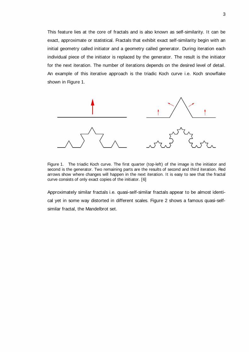
This feature lies at the core of fractals and is also known as self-similarity. It can be

exact, approximate or statistical. Fractals that exhibit exact self-similarity begin with an

initial geometry called initiator and a geometry called generator. During iteration each

individual piece of the initiator is replaced by the generator. The result is the initiator

for the next iteration. The number of iterations depends on the desired level of detail.

An example of this iterative approach is the triadic Koch curve i.e. Koch snowflake

shown in Figure 1.

Figure 1. The triadic Koch curve. The first quarter (top-left) of the image is the initiator and second is the generator. Two remaining parts are the results of second and third iteration. Red arrows show where changes will happen in the next iteration. It is easy to see that the fractal curve consists of only exact copies of the initiator. [6]

Approximately similar fractals i.e. quasi-self-similar fractals appear to be almost identi-

cal yet in some way distorted in different scales. Figure 2 shows a famous quasi-self-

similar fractal, the Mandelbrot set.

4

Figure 2. The quasi-self-similar Mandelbrot set. The fractal is looked at four different scales. The red square defines the area of observation at the next level of magnification. Different im-ages look very much the same yet none of them is exactly similar to any other but a variation of the same theme. [7]

Statistical self-similarity means that fractal has some kind of measures which are pre-

served across all scales. Real world coastlines fall to this category: a coastline looks like

a coastline no matter what the scale is, but it's impossible to find the large scale coast-

line repeating in the smaller scale coastlines neither exactly nor approximately similar.

Completely synthetic fractal based landscapes are very fast to generate and the re-

quired algorithms are relatively simple when compared to generating landscapes with

methods based on some physical process such as erosion or plate tectonics. They're

very efficient to store in memory because they can be restored from scratch if the ini-

tial seed is known. The coastal lines in fractal landscapes are very impressive and real-

istic, which is yet another reason for using fractals to generate random terrain. Howev-

er they possess a few serious flaws.

5

The biggest problem with fractals is expressed in their very definition. Self-similarity

means that a person looking at computer generated fractals soon sees the repetition

even if it is sometimes hard to point out. Computer generated landscapes quickly lose

their charm and become dull and repetitive in the eyes of the beholder unless signifi-

cant amount of post processing is applied to the generated heightmap. From the topo-

graphical point of view another major flaw with fractal landscapes is that the highest

mountains and deepest trenches nearly always lay at the center of the land of water

body. Figure 3 below shows many of these above mentioned properties of fractal ter-

rains.

Figure 3. A fractal terrain generated with diamond-square algorithm [8]. Orange text shows the scaling factor at each step. Red square signifies the area that's being zoomed into.

6

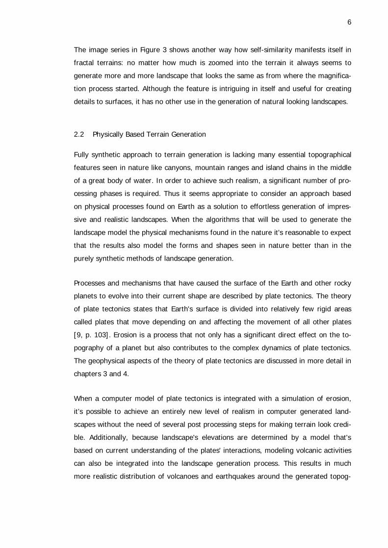
The image series in Figure 3 shows another way how self-similarity manifests itself in

fractal terrains: no matter how much is zoomed into the terrain it always seems to

generate more and more landscape that looks the same as from where the magnifica-

tion process started. Although the feature is intriguing in itself and useful for creating

details to surfaces, it has no other use in the generation of natural looking landscapes.

2.2 Physically Based Terrain Generation

Fully synthetic approach to terrain generation is lacking many essential topographical

features seen in nature like canyons, mountain ranges and island chains in the middle

of a great body of water. In order to achieve such realism, a significant number of pro-

cessing phases is required. Thus it seems appropriate to consider an approach based

on physical processes found on Earth as a solution to effortless generation of impres-

sive and realistic landscapes. When the algorithms that will be used to generate the

landscape model the physical mechanisms found in the nature it's reasonable to expect

that the results also model the forms and shapes seen in nature better than in the

purely synthetic methods of landscape generation.

Processes and mechanisms that have caused the surface of the Earth and other rocky

planets to evolve into their current shape are described by plate tectonics. The theory

of plate tectonics states that Earth's surface is divided into relatively few rigid areas

called plates that move depending on and affecting the movement of all other plates

[9, p. 103]. Erosion is a process that not only has a significant direct effect on the to-

pography of a planet but also contributes to the complex dynamics of plate tectonics.

The geophysical aspects of the theory of plate tectonics are discussed in more detail in

chapters 3 and 4.

When a computer model of plate tectonics is integrated with a simulation of erosion,

it’s possible to achieve an entirely new level of realism in computer generated land-

scapes without the need of several post processing steps for making terrain look credi-

ble. Additionally, because landscape's elevations are determined by a model that's

based on current understanding of the plates' interactions, modeling volcanic activities

can also be integrated into the landscape generation process. This results in much

more realistic distribution of volcanoes and earthquakes around the generated topog-

7

raphy than is possible when relying only on purely synthetic approaches. Plate tecton-

ics on Earth has not stopped yet and guesses have been made on how the topography

will change during the next hundreds of millions of years. Likewise a terrain generation

process that simulates plate tectonics can continue even while the landscape is being

used e.g. in a game.

However there is a price to pay for enhanced realism in the form of possibly highly

increased computational and algorithmic complexity. Simulating the movement, colli-

sions and deformations of so many plates will result in a potentially significant rise in

the processing time requirements. More complicated algorithms will take more devel-

oping time than fractal methods that are widely used, well known and usually fit into

one method or class. It is also probable that the coastal lines will not be as detailed

when simulating plate tectonics than when using fractal based methods. Additionally

it's certain that one cannot zoom into a landscape generated by plate tectonics without

a quick and sharp decrease in the level of detail. However the most serious obstacle in

the utilization of plate tectonics and erosion in the generation of landscapes is that it's

extremely hard to find any earlier work where it has been done. Thus it is difficult to

determine how much realism can be implemented into a model that ought to run on a

personal computer. The few projects that aim or have aimed to use plate tectonics

and/or erosion to generate landscapes are briefly reviewed in chapter 6.

8

3 Structure of Earth

Plate tectonics is the theory that explains how the outermost shell of the Earth is and

still continues to be, formed, deformed and destroyed around the planet. Factors un-

der, inside and above the outermost shell have an effect on the resulting topography

but of all these forces those that lie under the surface are the most meaningful. Thus

in order to model plate tectonics at any decent accuracy and level of realism it is nec-

essary to be familiar with both the structure of the Earth, mechanisms that act beneath

the surface and geological processes that take place at or very near the surface.

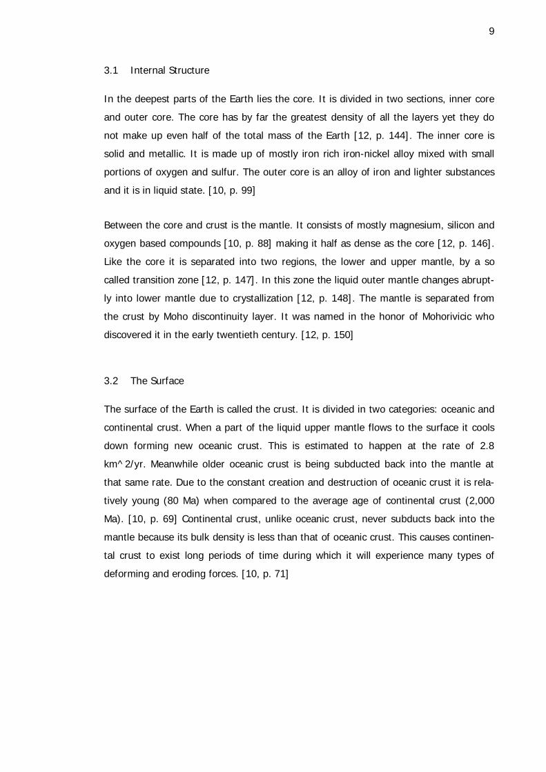
The inner structure of the Earth is divided into three major components: crust, mantle

and core. Mantle is subdivided into upper and lower mantle and core into outer and

inner core. These regions are layered on top of each other starting from the inner core

and ending with the crust (Figure 4). This spherical structure of the Earth was readily

available in 1940 [10, p. 63].

Figure 4. Regions of the Earth's interior. [11]

The majority of the mechanics of plate tectonics takes place in lithosphere which in-

cludes the crust and some of the upper mantle [12, p. 161]. As seen from Figure 4

they make up but a small fraction of the entire planet.

9

3.1 Internal Structure

In the deepest parts of the Earth lies the core. It is divided in two sections, inner core

and outer core. The core has by far the greatest density of all the layers yet they do

not make up even half of the total mass of the Earth [12, p. 144]. The inner core is

solid and metallic. It is made up of mostly iron rich iron-nickel alloy mixed with small

portions of oxygen and sulfur. The outer core is an alloy of iron and lighter substances

and it is in liquid state. [10, p. 99]

Between the core and crust is the mantle. It consists of mostly magnesium, silicon and

oxygen based compounds [10, p. 88] making it half as dense as the core [12, p. 146].

Like the core it is separated into two regions, the lower and upper mantle, by a so

called transition zone [12, p. 147]. In this zone the liquid outer mantle changes abrupt-

ly into lower mantle due to crystallization [12, p. 148]. The mantle is separated from

the crust by Moho discontinuity layer. It was named in the honor of Mohorivicic who

discovered it in the early twentieth century. [12, p. 150]

3.2 The Surface

The surface of the Earth is called the crust. It is divided in two categories: oceanic and

continental crust. When a part of the liquid upper mantle flows to the surface it cools

down forming new oceanic crust. This is estimated to happen at the rate of 2.8

km^2/yr. Meanwhile older oceanic crust is being subducted back into the mantle at

that same rate. Due to the constant creation and destruction of oceanic crust it is rela-

tively young (80 Ma) when compared to the average age of continental crust (2,000

Ma). [10, p. 69] Continental crust, unlike oceanic crust, never subducts back into the

mantle because its bulk density is less than that of oceanic crust. This causes continen-

tal crust to exist long periods of time during which it will experience many types of

deforming and eroding forces. [10, p. 71]

10

4 Plate Boundaries and the Wilson Cycle

New crust is being formed constantly. When two plates diverge hot magma erupts to

the surface. As it cools down new sea floor is formed and the body of water between

the diverging plates grows larger. At the same time somewhere else continental crust

collides and lumps up to form larger and larger continents. This causes the former

sea(s) that existed between colliding continents to disappear.

This concept of cyclic plate convergence and divergence is known as the Wilson cycle.

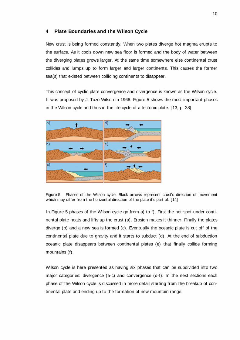
It was proposed by J. Tuzo Wilson in 1966. Figure 5 shows the most important phases

in the Wilson cycle and thus in the life cycle of a tectonic plate. [13, p. 38]

Figure 5. Phases of the Wilson cycle. Black arrows represent crust's direction of movement which may differ from the horizontal direction of the plate it's part of. [14]

In Figure 5 phases of the Wilson cycle go from a) to f). First the hot spot under conti-

nental plate heats and lifts up the crust (a). Erosion makes it thinner. Finally the plates

diverge (b) and a new sea is formed (c). Eventually the oceanic plate is cut off of the

continental plate due to gravity and it starts to subduct (d). At the end of subduction

oceanic plate disappears between continental plates (e) that finally collide forming

mountains (f).

Wilson cycle is here presented as having six phases that can be subdivided into two

major categories: divergence (a-c) and convergence (d-f). In the next sections each

phase of the Wilson cycle is discussed in more detail starting from the breakup of con-

tinental plate and ending up to the formation of new mountain range.

11

4.1 Divergent Plate Boundaries

Continental plate that's stationary with respect to the hotspot(s) below it has the po-

tential to split into Y-shaped or "three-armed" rift system due to the activity of the un-

derlying hot spot. Initially the hot spot causes the crust to arch up above it. This ex-

poses the continental crust to increased amounts of erosion which makes the crust

thinner. Finally the uplifted area splits into a three-armed rift system. All the arms meet

at the hot spot's location and extend away from each other. At the center of an "arm"

in the drift system is a block of crust that has dropped down to accommodate the hori-

zontal extension of the continent. This down-dropped block is known as graben (Figure

6). [12, p. 310-312]

Figure 6. Graben is the sinking central part of a rift valley. The rift valley is the area of re-duced elevation between two diverging continental plates. [15]

If the process continues, the continent splits up along two arms of the rift system due

to varying tensional stresses applied to it by other plates and gravity. This eventually

leads to the birth of a new "seafloor-spreading center, or ridge" which is illustrated in

figures Figure 6 and Figure 7. [13, p. 38]

12

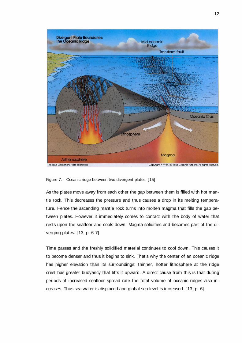
Figure 7. Oceanic ridge between two divergent plates. [15]

As the plates move away from each other the gap between them is filled with hot man-

tle rock. This decreases the pressure and thus causes a drop in its melting tempera-

ture. Hence the ascending mantle rock turns into molten magma that fills the gap be-

tween plates. However it immediately comes to contact with the body of water that

rests upon the seafloor and cools down. Magma solidifies and becomes part of the di-

verging plates. [13, p. 6-7]

Time passes and the freshly solidified material continues to cool down. This causes it

to become denser and thus it begins to sink. That’s why the center of an oceanic ridge

has higher elevation than its surroundings: thinner, hotter lithosphere at the ridge

crest has greater buoyancy that lifts it upward. A direct cause from this is that during

periods of increased seafloor spread rate the total volume of oceanic ridges also in-

creases. Thus sea water is displaced and global sea level is increased. [13, p. 6]

13

When a continent splits up and the individual pieces begin to diverge the first pieces of

seafloor are formed. As time passes and continents continue on their tracks away from

each other the initial segments of new seafloor become colder, denser and thicker.

Gradually their density surpasses that of the underlying mantle rock and lithosphere

becomes gravitationally unstable. (Figure 5, part c) As a result of this the old and

heavy lithosphere starts to subside from the continental crust. Finally the seafloor

breaks off of the continent and starts to sink into the mantle. This is the birth of a new

ocean trench (Figure 5, part d). [13, p. 9]

4.2 Convergent Plate Boundaries

4.2.1 Oceanic Plates

Ocean trench is a location where oceanic plate subducts under continental plate. After

oceanic lithosphere has become cool and dense it begins to sink into the mantle. Even-

tually this subducting lithosphere encounters mantle rock that is denser than what the

lithosphere was on the surface planet. However the increase of pressure deeper in the

mantle causes also the lithosphere to become increasingly dense up to the point where

it is denser than its surroundings. Consequently the subduction process continues until

descending lithosphere melts away and becomes part of the same mantle it originated

from. [13, p. 9]

The subduction of oceanic plate is accompanied by strong seismic activity. Earthquakes

in the so called shallow zone which ranges from surface to 100 km in depth originate

from the boundary between plates and are the result of friction between the descend-

ing plate and the overlying plate. Quakes in intermediate depths (between 100 and

300 km) are originated from within the subducting plate itself. They are the result of

extension and compression that the subducting lithosphere undergoes. Finally in

depths ranging from 300 to 700 km the descending lithosphere encounters material

that resists its movement. This causes so called deep zone earthquakes. [12, p. 177-

178]

14

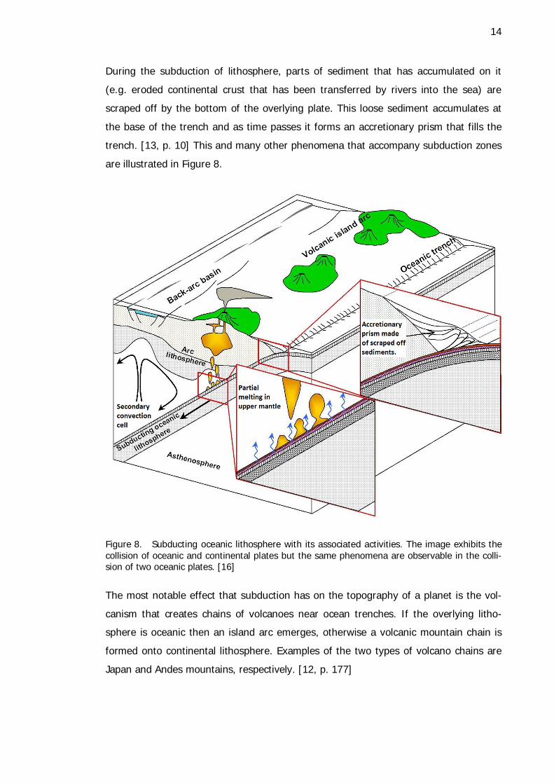
During the subduction of lithosphere, parts of sediment that has accumulated on it

(e.g. eroded continental crust that has been transferred by rivers into the sea) are

scraped off by the bottom of the overlying plate. This loose sediment accumulates at

the base of the trench and as time passes it forms an accretionary prism that fills the

trench. [13, p. 10] This and many other phenomena that accompany subduction zones

are illustrated in Figure 8.

Figure 8. Subducting oceanic lithosphere with its associated activities. The image exhibits the collision of oceanic and continental plates but the same phenomena are observable in the colli-sion of two oceanic plates. [16]

The most notable effect that subduction has on the topography of a planet is the vol-

canism that creates chains of volcanoes near ocean trenches. If the overlying litho-

sphere is oceanic then an island arc emerges, otherwise a volcanic mountain chain is

formed onto continental lithosphere. Examples of the two types of volcano chains are

Japan and Andes mountains, respectively. [12, p. 177]

15

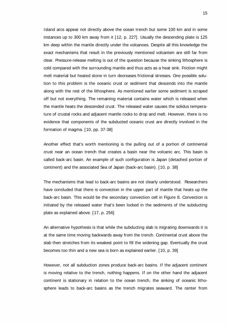
Island arcs appear not directly above the ocean trench but some 100 km and in some

instances up to 300 km away from it [12, p. 227]. Usually the descending plate is 125

km deep within the mantle directly under the volcanoes. Despite all this knowledge the

exact mechanisms that result in the previously mentioned volcanism are still far from

clear. Pressure-release melting is out of the question because the sinking lithosphere is

cold compared with the surrounding mantle and thus acts as a heat sink. Friction might

melt material but heated stone in turn decreases frictional stresses. One possible solu-

tion to this problem is the oceanic crust or sediment that descends into the mantle

along with the rest of the lithosphere. As mentioned earlier some sediment is scraped

off but not everything. The remaining material contains water which is released when

the mantle heats the descended crust. The released water causes the solidus tempera-

ture of crustal rocks and adjacent mantle rocks to drop and melt. However, there is no

evidence that components of the subducted oceanic crust are directly involved in the

formation of magma. [10, pp. 37-38]

Another effect that's worth mentioning is the pulling out of a portion of continental

crust near an ocean trench that creates a basin near the volcanic arc. This basin is

called back-arc basin. An example of such configuration is Japan (detached portion of

continent) and the associated Sea of Japan (back-arc basin). [10, p. 38]

The mechanisms that lead to back-arc basins are not clearly understood. Researchers

have concluded that there is convection in the upper part of mantle that heats up the

back-arc basin. This would be the secondary convection cell in Figure 8. Convection is

initiated by the released water that's been locked in the sediments of the subducting

plate as explained above. [17, p. 256]

An alternative hypothesis is that while the subducting slab is migrating downwards it is

at the same time moving backwards away from the trench. Continental crust above the

slab then stretches from its weakest point to fill the widening gap. Eventually the crust

becomes too thin and a new sea is born as explained earlier. [10, p. 39]

However, not all subduction zones produce back-arc basins. If the adjacent continent

is moving relative to the trench, nothing happens. If on the other hand the adjacent

continent is stationary in relation to the ocean trench, the sinking of oceanic litho-

sphere leads to back-arc basins as the trench migrates seaward. The center from

16

where back-arc basin will start to spread has been observed to be located at the vol-

canic lines which are the weakest portion of the adjacent continental crust due to

magma flow through it. [13, p. 13]

Seas that are surrounded by continents exist as long as the equilibrium between rate

of subduction and seafloor spreading holds. As soon as the surrounding continents

start to draw closer to each other the sea between them will start to shrink (Figure 5,

part e). If nothing changes the eventual outcomes are the disappearance of the sea,

the subduction of the oceanic ridge and the collision of continents (Figure 5, part f),

which is discussed in the next section.

4.2.2 Continental Plates

The collision of two continents is very different from a collision between oceanic and

continental lithosphere. Continental crust is too thick and too buoyant to sink back to

the mantle like oceanic lithosphere does and therefore it remains at the outer surface

of the planet much longer. Eventually the ever afloat continents will collide with spec-

tacular consequences. Himalayas, that contain the highest mountains in world, are the

result of the Indian plate colliding with the continental plate of Asia. Another example

of a collision of two continents is the Alpine mountain belt. It is the result of the African

plate colliding with the European plate. [12, p. 278-281] The building of mountains

during continental collision is called orogeny and the area where mountains grow is

orogenic zone [13, p. 41].

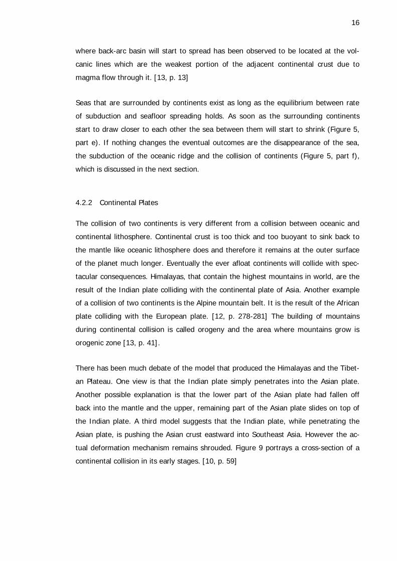
There has been much debate of the model that produced the Himalayas and the Tibet-

an Plateau. One view is that the Indian plate simply penetrates into the Asian plate.

Another possible explanation is that the lower part of the Asian plate had fallen off

back into the mantle and the upper, remaining part of the Asian plate slides on top of

the Indian plate. A third model suggests that the Indian plate, while penetrating the

Asian plate, is pushing the Asian crust eastward into Southeast Asia. However the ac-

tual deformation mechanism remains shrouded. Figure 9 portrays a cross-section of a

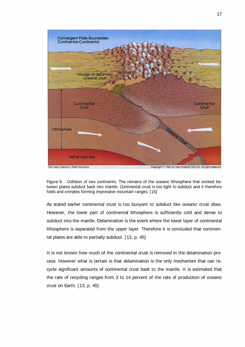
continental collision in its early stages. [10, p. 59]

17

Figure 9. Collision of two continents. The remains of the oceanic lithosphere that existed be-tween plates subduct back into mantle. Continental crust is too light to subduct and it therefore folds and crimples forming impressive mountain ranges. [15]

As stated earlier continental crust is too buoyant to subduct like oceanic crust does.

However, the lower part of continental lithosphere is sufficiently cold and dense to

subduct into the mantle. Delamination is the event where the lower layer of continental

lithosphere is separated from the upper layer. Therefore it is concluded that continen-

tal plates are able to partially subduct. [13, p. 45]

It is not known how much of the continental crust is removed in the delamination pro-

cess. However what is certain is that delamination is the only mechanism that can re-

cycle significant amounts of continental crust back to the mantle. It is estimated that

the rate of recycling ranges from 3 to 14 percent of the rate of production of oceanic

crust on Earth. [13, p. 45]

18

Continental collision produces significant amounts of horizontal stress to the crust. In

brittle crust this causes compression and thickening in the form of thrust faults as illus-

trated in Figure 10. A location where many thrust faults occur next to each other is

called thrust belt. There the rising blocks constitute a mountain range. Valleys form

between them. [13, p. 42]

Figure 10. A thrust fault. Many thrust faults one after another form a thrust belt. [18]

Deformation of ductile crust during continental collision results in folding. This is de-

picted in Figure 11. When a region of the soft layers of soil erodes away it fills the bot-

toms of the fold creating valleys. The hard stone underneath the soil resists erosion

and forms ridges that separate valleys from each other. [13, p. 45]

Figure 11. Folding of ductile crust. The soft soil at the top of fold has eroded away and fallen to the groove (brown area). [19]

19

Continental convergence is the end of the Wilson cycle (Figure 5, part f). Although this

cycle has long been thought to be continuous processes where old crust is absorbed

and new is formed constantly, researchers from Carnegie Institution of Washington

and Woods Hole Oceanographic Institution (WHOI) have recently suggested that plate

tectonics might be periodically turned off. When all continents gather into one lump

forming what is known as supercontinent, subduction effectively ceases. This in turn

reduces the amount of heat released from the interiors of Earth into space possibly

explaining the large amounts of heat Earth still releases today. [20]

Additionally the collision of continents, like collision of oceanic lithospheres, is accom-

panied by earthquakes. However earthquakes also emerge when plates merely slide

past one another. These areas are called transform faults.

4.3 Transform Faults

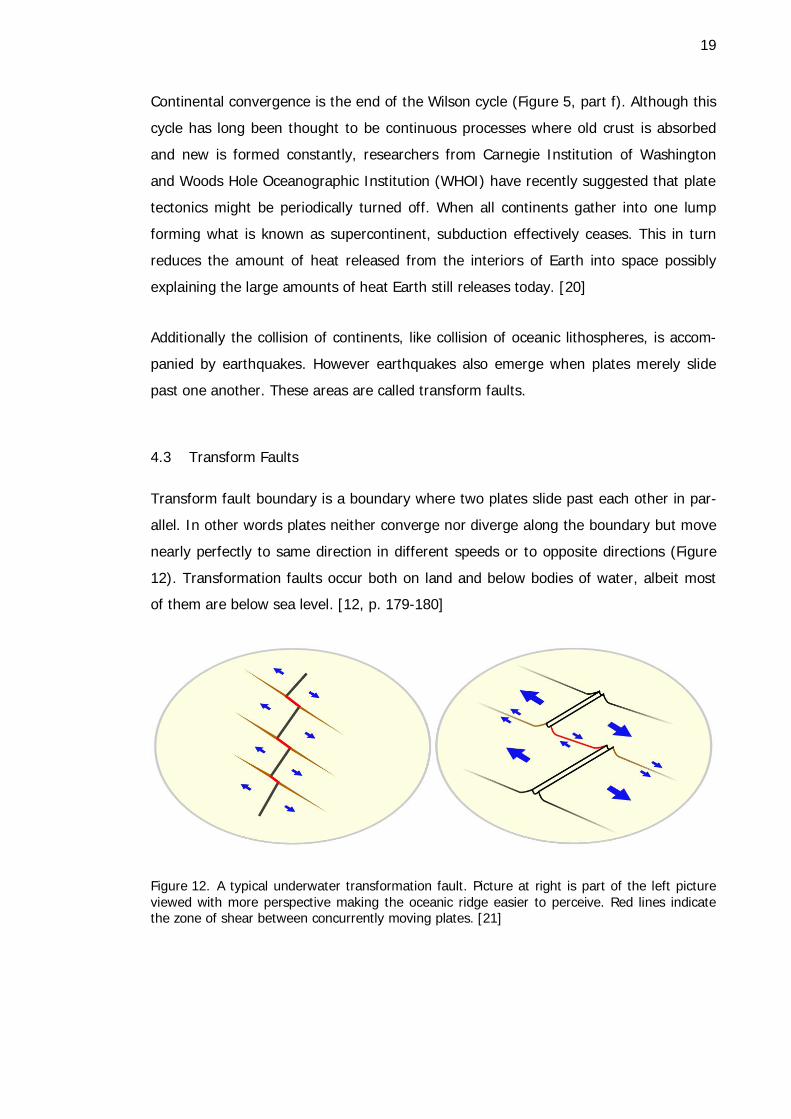
Transform fault boundary is a boundary where two plates slide past each other in par-

allel. In other words plates neither converge nor diverge along the boundary but move

nearly perfectly to same direction in different speeds or to opposite directions (Figure

12). Transformation faults occur both on land and below bodies of water, albeit most

of them are below sea level. [12, p. 179-180]

Figure 12. A typical underwater transformation fault. Picture at right is part of the left picture viewed with more perspective making the oceanic ridge easier to perceive. Red lines indicate the zone of shear between concurrently moving plates. [21]

20

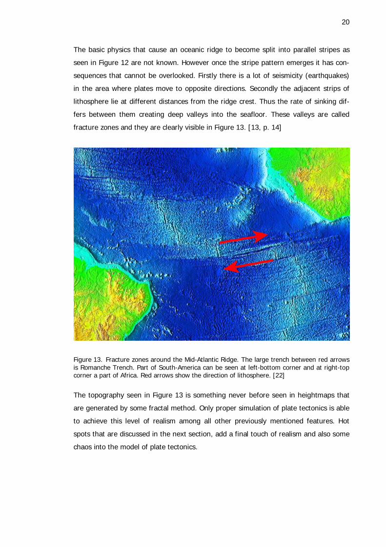
The basic physics that cause an oceanic ridge to become split into parallel stripes as

seen in Figure 12 are not known. However once the stripe pattern emerges it has con-

sequences that cannot be overlooked. Firstly there is a lot of seismicity (earthquakes)

in the area where plates move to opposite directions. Secondly the adjacent strips of

lithosphere lie at different distances from the ridge crest. Thus the rate of sinking dif-

fers between them creating deep valleys into the seafloor. These valleys are called

fracture zones and they are clearly visible in Figure 13. [13, p. 14]

Figure 13. Fracture zones around the Mid-Atlantic Ridge. The large trench between red arrows is Romanche Trench. Part of South-America can be seen at left-bottom corner and at right-top corner a part of Africa. Red arrows show the direction of lithosphere. [22]

The topography seen in Figure 13 is something never before seen in heightmaps that

are generated by some fractal method. Only proper simulation of plate tectonics is able

to achieve this level of realism among all other previously mentioned features. Hot

spots that are discussed in the next section, add a final touch of realism and also some

chaos into the model of plate tectonics.

21

5 Other Influential Mechanisms

Even though interactions between plates are the cause of most notable alterations in

planet's topography, there are a few more phenomena that must be considered when

plate tectonics is discussed. One of them is represented by a lonely volcano far away

from any convergent plate boundaries. These hot spots, as they're called, rise from the

depths of the Earth and time passing they create chains of mountains that add promi-

nent details to a landscape.

Like hot spots, erosion also has an undeniable effect on landscapes. Wind, waters and

temperature variations all contribute to the diverse family of mechanisms that cause

materials to erode. Tall mountains are erased to flat hills and steep ravines become

gently sloping valleys. These and other phenomena are briefly discussed in the follow-

ing sections.

5.1 Hot spots

A hot spot is an area of abnormally high volcanism that cannot be explained by plate

tectonic processes alone. A hot spot may or may not be part of a plate boundary pro-

cess such as divergence or subduction. In the former case a good example would be

Hawaii that's located nearly at the center of the Pacific plate. Iceland is an example of

a case where a hot spot is located at the boundary of two divergent plates. There it

contributes to the formation of new oceanic crust and this causes the crust to become

anomalously thick and the ocean ridge anomalously elevated. [10, p. 499]

During the last 10 million years there have existed at least 122 hot spots [17, p. 249].

The definition of a hot spot is still quite subjective and thus there exists many opinions

on the exact number of identified hot spots. Despite the vagueness some of the most

prominent hot spots are seen in Figure 14.

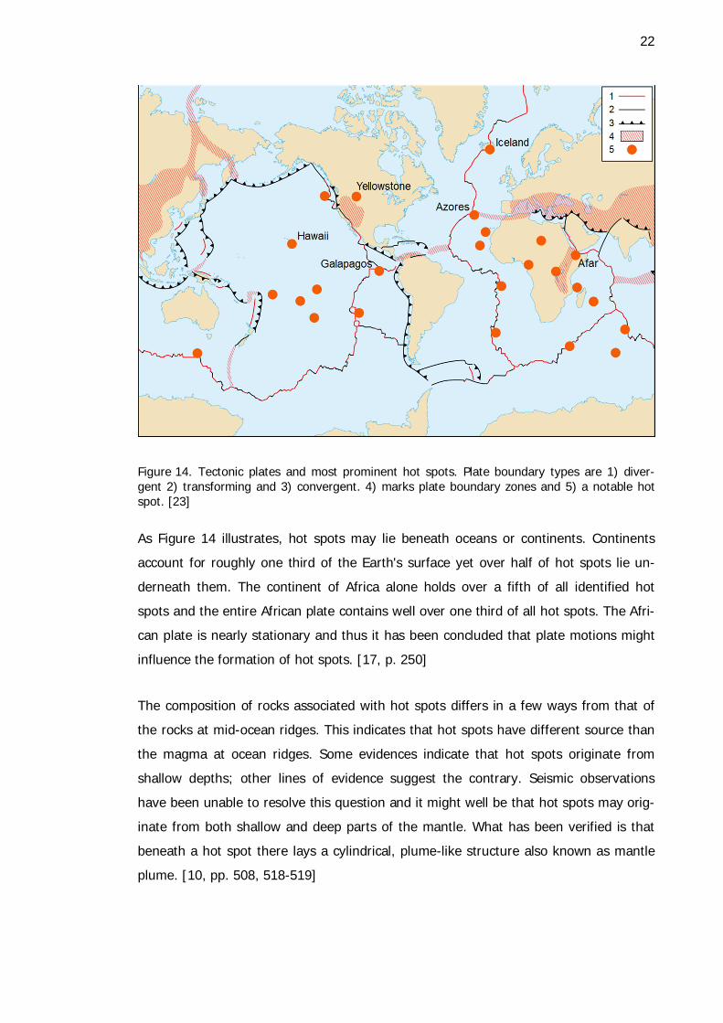
22

Figure 14. Tectonic plates and most prominent hot spots. Plate boundary types are 1) diver-gent 2) transforming and 3) convergent. 4) marks plate boundary zones and 5) a notable hot spot. [23]

As Figure 14 illustrates, hot spots may lie beneath oceans or continents. Continents

account for roughly one third of the Earth's surface yet over half of hot spots lie un-

derneath them. The continent of Africa alone holds over a fifth of all identified hot

spots and the entire African plate contains well over one third of all hot spots. The Afri-

can plate is nearly stationary and thus it has been concluded that plate motions might

influence the formation of hot spots. [17, p. 250]

The composition of rocks associated with hot spots differs in a few ways from that of

the rocks at mid-ocean ridges. This indicates that hot spots have different source than

the magma at ocean ridges. Some evidences indicate that hot spots originate from

shallow depths; other lines of evidence suggest the contrary. Seismic observations

have been unable to resolve this question and it might well be that hot spots may orig-

inate from both shallow and deep parts of the mantle. What has been verified is that

beneath a hot spot there lays a cylindrical, plume-like structure also known as mantle

plume. [10, pp. 508, 518-519]

23

Hot spots are typically accompanied by topographic swells. Their shape is roughly par-

abolic creating up to 3 km excess elevation around the hot spot. Their cause is still

somewhat controversial. Some suggest that the heated material rising along the man-

tle plume makes the lithosphere thinner and that as lithosphere moves away from the

hot spot center it cools down and thickens again. However, the theory contradicts

some measurements. [10, pp. 505-507]

Another hypothesis is that the hot and thus buoyant plume material lifts up the litho-

sphere. As the material rises along the mantle plume, it eventually impinges on the

lithosphere. The pipe like plume flow starts to spread beneath the resisting lithosphere

forming a mushroom-shaped cap at the top of the mantle plume. This causes pressure

against the lithosphere. The highest pressure is naturally at the center of the swell and

it gradually weakens when moving further from the hot spot. Because the strength of

the mantle flow of a hot spot varies from time to time, the evolution observed in hot

spot swells can be explained without the need of lithospheric thinning. [10, p. 507]

When the mantle plume eventually breaks through the lithosphere, it does so with

much fierce. The volume of the surfacing magma in the initial eruption is at least half

of the total volume that hot spot produces during its existence. There have been also

observations that after the first third of its life the hot spot erupts ferociously again.

This might be explained by a secondary plume head that forms in very narrow trailing

conduits. [10, pp. 527-528]

Once formed the hot spot remains relatively stationary. In other words hot spots ap-

pear to be fixed with respect to the mantle. However, they are not precisely fixed but

move at speeds that are significantly slower than that of any oceanic or continental

lithosphere. The question of hot spot movement is further blurred by variations in ac-

tivity pattern between hot spots. Some of them produce segmented tracks; others are

active only in short pulses. There are also hot spots that have active volcanism simul-

taneously at several sites. For these the idea of approximate stationarity is less rele-

vant. [10, pp. 501-502]

When a plate moves over the practically stationary hot spot, it leaves behind a nearly

linear track of volcanic islands and seamounts. This is illustrated in Figure 15.

24

Figure 15. Relatively stationary hot spot forms a volcanic mountain chain on the plate above it. [15]

When the overlying plate moves it drags the vent further away from the center of the

hot spot. Eventually the magma pipe breaks and volcanism ceases at the mount. Be-

cause no new crust is being added to it anymore, erosion is free to wear it out. As the

island ages it becomes lower and turns into underwater sea mount. Meanwhile the

mantle plume has penetrated the lithosphere right at the center of the hot spot and a

new volcano is formed. A classical prototype of this process is the Hawaiian-Emperor

chain show in Figure 16.

25

Figure 16. The Hawaii-Emperor seamount chain. [24]

The near-linearity of the volcanic chain generated by the hot spot is easily perceivable

in Figure 16, as is the variation in the hot spot's rate of volcanism. Hawaiian and Em-

peror Chains would be one long, straight track had not the pole of rotation of Pacific

plate changed due to a collision between the Asian and Indian plates 43 million years

ago. [10, p. 501]

Hot spots are not permanent but rather transient features, i.e. they fade away sooner

or later. A typical life span of a hot spot is around 100 million years. However new

plumes are constantly formed as previous wear out and thus the heat flux system as a

whole could be considered as a permanent feature of the Earth. [25, p. 93]

26

5.2 Erosion

Crust not covered by seas or other large bodies of water is subject to many forms of

outwearing and erosion. The Sun's thermal energy results in chemical activity and

temperature variations. Gravitation pulls crust downward and forces streams of water

to flow downhill wearing out everything on their way. However, below sea level winds

don't blow, temperature changes are far slower and gravitation has a diminished effect

due to support of the surrounding water. [12, p. 346]

The wearing down of land can be divided to three kinds of processes. Firstly there's

weathering, the fragmentation and disintegration of the original rock into smaller com-

ponents. Secondly there's erosion, which is the removal and transportation of rock de-

bris. Finally there's mass wasting, which, as defined in [12],

"refers to the gravitational downward movement of rock fragments without the involvement of a transporting medium such as water."

However in this text they are all capped under the term erosion, because it's probably

the best understood word among common people for all the processes described

above.

The forms of erosion are manifold. As mentioned earlier, temperature variations may

fragment stone into smaller pieces. During days the Sun heats stone and makes it ex-

pand. After sunset the absorbed heat evaporates swiftly and stone contracts. Eventual-

ly it breaks into two smaller pieces. However, laboratory experiments have failed to

reproduce this phenomenon. [12, p. 350]

Wind, although easier to notice, is nevertheless a weaker eroding force than heat flux-

es. It acts mainly as transporter of material in the form of sand and snow storms in

areas where vegetation is sparse or completely lacking. Transported material accumu-

lates forming dunes and loess. In dunes the crumbs of land are free and in loess

they're suspended together. [12, pp. 417-422]

However, by far the most important component in the wearing down of land is water.

This is because its mass is far greater than that of air. Rain moves grains of land ef-

fortlessly creating destructive mudflows [12, p. 382]. It gradually washes off soil un-

27

protected by vegetation [12, p. 393]. Drops of water come together forming brooks,

streams and rivers that erode the land wherever they run. These flows create furrows

to mountains giving them their distinctive shape. Rivers are also capable of transport-

ing large quantities of soil ranging from small crumbs to large boulders of stone [12, p.

401].

Eventually all this loose sediment ends up to sea with the water transporting it. Seas

fill the basins left between two diverging plates. Their waves continuously dash against

the shores eating the land away piece by piece [12, p. 335].

Many more things cause erosion. Plants remove nutrient ions directly from the soil and

bacteria release organic acids that become involved in the chemical weathering reac-

tions in the soil [12, p. 359]. Water that freezes within the cracks of a rock exerts

pressure that causes it to disintegrate [12, p. 350].

In colder regions snow accumulates to form large, thick blankets of ice called glaciers

[12, p. 429]. They are capable of moving very large rocks due to their crystalline na-

ture [12, p. 429]. The glaciers grind, scrape and pluck the crust underneath them re-

sulting in various deformations and loss of rock material [12, p. 436]. Times of excep-

tional global coolness result in gigantic ice sheets that take up large quantities of water

lowering the sea level and exposing fresh land to erosion. When ice sheets melt, the

sea level raises again flooding low lying areas [12, p. 467]. Last, but not least, is the

erosion caused by activities of man. It has been estimated that since the beginning of

agriculture man has more than doubled the average amount of soil that's eroded into

the world's rivers [12, p. 470]!

From the descriptions above it is easy to see that climate has a remarkably big role in

the formation of planet's topography. It is well known that e.g. closure of an ocean

basin or building of mountain affects the climate, but quite recently the opposite has

also been shown to be true. An Australian-led team of researchers have discovered

that the strengthened monsoon in India has accelerated the movement of the Indian

plate over the past 10 million years [26]. This finding reveals a feedback mechanism to

the motion of plates and thus it is deduced that an appropriate simulation of erosion is

an integral part of any serious plate tectonic model.

28

5.3 Isostasy

As stated in the previous chapter, there is less erosion under water than on bare

ground above sea level. Of all the dry land young mountain belts are the ones that

have the greatest rate of erosion [10, p. 560]. Mountains erode to near sea level in

mere 50 million years which is relatively short in geologic terms [10, p.72]. However as

erosion removes crust from the mountain and transports it elsewhere, the continental

crust rises, compensating for the reduction in height. This phenomenon is called iso-

static uplift and will be described in greater detail below.

Continents and crust in general are floating over the mantle like blocks of wood or ice

in water. The buoyancy of crust is due to its smaller density in comparison to the man-

tle. As stated in [13], continents

"are buoyed up by a force equal to the weight of the mantle rock displaced."

in accordance to Archimedes' principle. Hydrostatic principle states that the amount of

stress that a continent places on the mantle as it partially "sinks" into it is equal to the

uplift that the mantle exerts to the "sinking" crust. [13, p. 74].

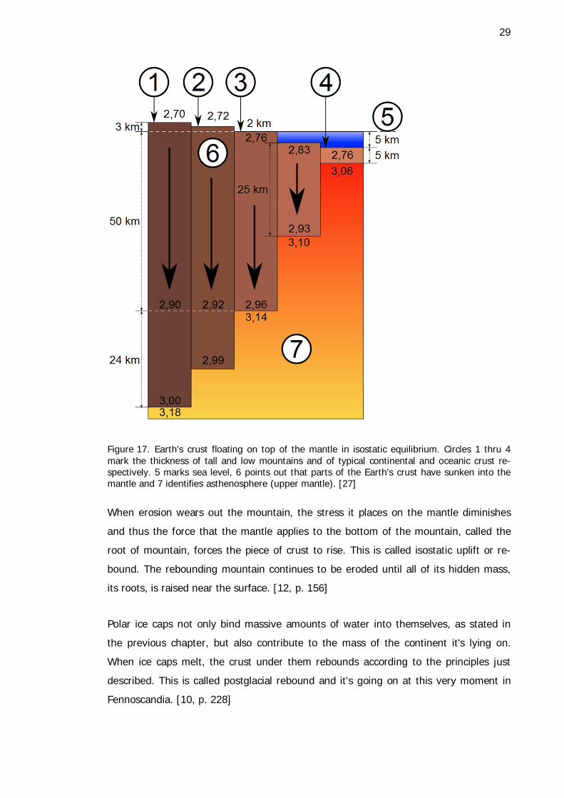
Therefore, the "taller" the pile of crust, the deeper it sinks. Like ice cubes or icebergs

floating on top of water, only their tip is visible and most of their mass is hidden be-

neath the surface. Figure 17 illustrates how this principle is manifested on Earth.

29

Figure 17. Earth's crust floating on top of the mantle in isostatic equilibrium. Circles 1 thru 4 mark the thickness of tall and low mountains and of typical continental and oceanic crust re-spectively. 5 marks sea level, 6 points out that parts of the Earth's crust have sunken into the mantle and 7 identifies asthenosphere (upper mantle). [27]

When erosion wears out the mountain, the stress it places on the mantle diminishes

and thus the force that the mantle applies to the bottom of the mountain, called the

root of mountain, forces the piece of crust to rise. This is called isostatic uplift or re-

bound. The rebounding mountain continues to be eroded until all of its hidden mass,

its roots, is raised near the surface. [12, p. 156]

Polar ice caps not only bind massive amounts of water into themselves, as stated in

the previous chapter, but also contribute to the mass of the continent it's lying on.

When ice caps melt, the crust under them rebounds according to the principles just

described. This is called postglacial rebound and it's going on at this very moment in

Fennoscandia. [10, p. 228]

30

6 Earlier Works

Projects that aim to generate heightmaps relying on plate tectonics seem to be ex-

tremely few and far between. After much of searching with the help of the Internet's

well known search engines only a handful of related works was found. Of those the

most relevant and promising are reviewed below.

6.1 Stella Polaris project

In the beginning of 2003 a nickname "Lemmy" started a thread in the Apolyton Civili-

zation Site asking people to share their opinions on the map generation algorithms

they've been using for some apparently two dimensional tile based game. One of the

most interesting replies were posted by nickname "Impaler[WrG]". In his post he de-

scribes an algorithm for terrain generation that he devised while working in the Stella

Polaris project. What's remarkable in it is that it emulates plate tectonics. Although the

development of the map generator halted before it was finished, the precursory results

seemed very promising. [28]

In his post Impaler[WrG] gives quite a detailed description on how the map generator

works. In short the algorithm first segments the initial heightmap into 6-12 "tectonic"

plates. Each plate is given a random direction and speed. The plates are moved in par-

allel according to their speed and direction. After all plates have moved, their interac-

tions are processed. If two plates overlap, the slower plate adopts the direction and

speed of the faster plate. This emulates the collision of two plates. If a plate leaves

behind it emptiness, a location where no plate lies, then that empty location is filled

with seafloor and attached to the first-mentioned plate. This emulates seafloor spread-

ing. The cycle of movement and interaction handling is repeated 20-30 times. Then

erosion algorithm is applied and the heightmap is updated to reflect the changes in the

plate system. The elevation of overlapping plates is simply added together. The updat-

ed heightmap is then segmented again with brand new plates and the entire process is

restarted. This cycle is repeated 3-4 times before the map generation process has

come to its conclusion. [28]

31

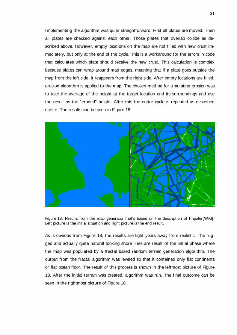
Implementing the algorithm was quite straightforward. First all plates are moved. Then

all plates are checked against each other. Those plates that overlap collide as de-

scribed above. However, empty locations on the map are not filled with new crust im-

mediately, but only at the end of the cycle. This is a workaround for the errors in code

that calculates which plate should receive the new crust. This calculation is complex

because plates can wrap around map edges, meaning that if a plate goes outside the

map from the left side, it reappears from the right side. After empty locations are filled,

erosion algorithm is applied to the map. The chosen method for simulating erosion was

to take the average of the height at the target location and its surroundings and use

the result as the "eroded" height. After this the entire cycle is repeated as described

earlier. The results can be seen in Figure 18.

Figure 18. Results from the map generator that's based on the description of Impaler[WrG]. Left picture is the initial situation and right picture is the end result.

As is obvious from Figure 18, the results are light years away from realistic. The rug-

ged and actually quite natural looking shore lines are result of the initial phase where

the map was populated by a fractal based random terrain generation algorithm. The

output from the fractal algorithm was leveled so that it contained only flat continents

or flat ocean floor. The result of this process is shown in the leftmost picture of Figure

18. After the initial terrain was created, algorithm was run. The final outcome can be

seen in the rightmost picture of Figure 18.

32

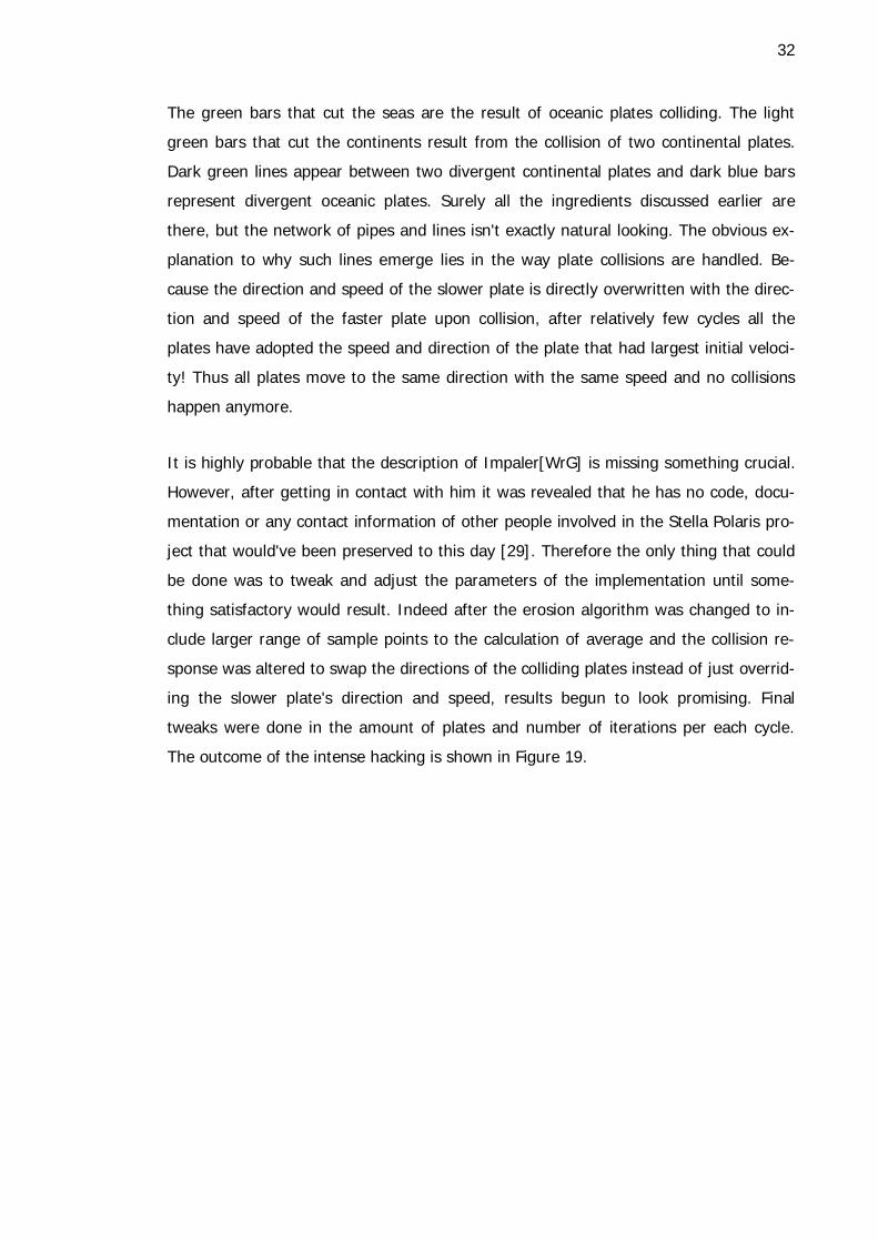
The green bars that cut the seas are the result of oceanic plates colliding. The light

green bars that cut the continents result from the collision of two continental plates.

Dark green lines appear between two divergent continental plates and dark blue bars

represent divergent oceanic plates. Surely all the ingredients discussed earlier are

there, but the network of pipes and lines isn't exactly natural looking. The obvious ex-

planation to why such lines emerge lies in the way plate collisions are handled. Be-

cause the direction and speed of the slower plate is directly overwritten with the direc-

tion and speed of the faster plate upon collision, after relatively few cycles all the

plates have adopted the speed and direction of the plate that had largest initial veloci-

ty! Thus all plates move to the same direction with the same speed and no collisions

happen anymore.

It is highly probable that the description of Impaler[WrG] is missing something crucial.

However, after getting in contact with him it was revealed that he has no code, docu-

mentation or any contact information of other people involved in the Stella Polaris pro-

ject that would've been preserved to this day [29]. Therefore the only thing that could

be done was to tweak and adjust the parameters of the implementation until some-

thing satisfactory would result. Indeed after the erosion algorithm was changed to in-

clude larger range of sample points to the calculation of average and the collision re-

sponse was altered to swap the directions of the colliding plates instead of just overrid-

ing the slower plate's direction and speed, results begun to look promising. Final

tweaks were done in the amount of plates and number of iterations per each cycle.

The outcome of the intense hacking is shown in Figure 19.

33

Figure 19. Output from the improved version of the Stella Polaris inspired terrain generator.

Like before, the initial situation is a flattened fractal based terrain and it is again the

reason for quite realistic shore lines. What is obvious from Figure 19 is that the new

erosion algorithm causes the map to become exceedingly blurred. Secondly, because

continents pack on top of each other faster than new seafloor is formed, the total

amount of dry land is reduced until equilibrium is reached. This results in a handful of

islands floating around the map.

While the results in the latter model were significantly better than in the initial version,

they both are still far away from the desired level of realism. Neither of them was able

to produce realistic mountain ranges nor island chains. They even fell behind ordinary

fractal based methods in simplicity, performance and amount of realism! Despite all

their shortcomings they still serve as an excellent starting point for the model that will

be described in great detail later.

34

6.2 Cdrift

In 1991 David Allen released the source code and related documentation of the conti-

nental drift simulator, climate generator and rectangle-onto-sphere mapping utility that

he had written in C for Amiga and UN*X environments. His motivation for doing all this

was that fractal methods produce too random and unnatural looking maps. [30]

His approach was to model the supercontinent cycle. According to him heat from the

Earth's interiors breaks large continents into fragments that drift around for a while.

Eventually they are drawn back together thus forming a new supercontinent. At some

point it too is broken into smaller pieces and the cycle repeats. [30]

Puzzled by the problem of mapping a rectangle onto a sphere and being restricted by

the computing power available to a private person back then, he decided to simulate

continental drift on a simple square. Crust that exceeds the square's dimensions is

simply removed from the system. A second simplification that he implemented was to

ignore ocean floor movement and subductions altogether. This was because of the way

he maintained the details of each continent that apparently made the representation of

ocean spreading centers too difficult. Because subducting ocean floor that drags conti-

nents back together doesn't exist in his system anymore, he added simple "spring" like

behavior to plates that causes them to eventually draw back together. [30]

His model starts out by creating a single supercontinent with a fractal based terrain

generating algorithm. During the iteration, some old continent, if it's big enough, is

split in two. The pieces receive new directions so that they will move away from each

other and new speeds so that the smaller continent moves faster than the larger.

Plates are then moved. If a plate moves over an ocean tile, land mass is added to the

plate's leading edge simulating subduction. If a plate moves over another plate, then

the collision counter between those plates is increased and land mass is added to one

of the plates simulating continental collision. The velocities of the colliding plates are

adjusted so that their relative speed diminishes. If it becomes smaller than some

threshold, the plates are merged together. Finally erosion is applied to the system and

the screen is redrawn. [30]

35

Despite the undeniable simplicity of David Allen's continental drift simulator, the results

are remarkably convincing as can be seen in Figure 20. Mountain ranges are formed

near the shores of drifting plates and between colliding continents. That is very im-

pressive for software nearly 21 years old!

Figure 20. Collection of 25 consecutive iterations of David Allen's Cdrift. Simulation starts from top-left corner and proceeds from left to right, top to bottom. [30]

However, there are undeniably some artifacts visible, mainly related to mountain rang-

es. Firstly, they seem to be everywhere. That is probably the product of quite aggres-

sive splitting of continents that leads to constant creation of new subduction and conti-

nental collision sites. The way continents are split is a problem in itself, for it leads to

artificially straight mountain ranges. Reducing the rate of continental splits reveals the

problems in erosion algorithm. The land area grows in a very unnatural looking way

and all minuscule details are lost resulting in a very blurry outcome.

David has made another version of his continent drift simulation that produces more

detailed and colorful heightmaps. All the source code and related documentation are

downloadable from [30]. The package is called Planet and it includes a continental drift

simulator, climate generator and rectangle-onto-sphere mapping utility that were men-

tioned at the beginning of this section. Of these only the continental drift simulator is

36

of great relevance to this thesis and thus the other software, although extremely intri-

guing in themselves, are ignored. The new version apparently uses the same mecha-

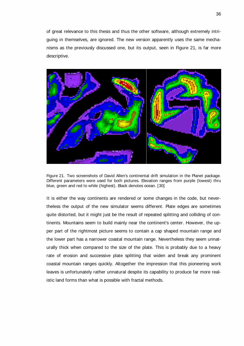
nisms as the previously discussed one, but its output, seen in Figure 21, is far more

descriptive.

Figure 21. Two screenshots of David Allen's continental drift simulation in the Planet package. Different parameters were used for both pictures. Elevation ranges from purple (lowest) thru blue, green and red to while (highest). Black denotes ocean. [30]

It is either the way continents are rendered or some changes in the code, but never-

theless the output of the new simulator seems different. Plate edges are sometimes

quite distorted, but it might just be the result of repeated splitting and colliding of con-

tinents. Mountains seem to build mainly near the continent's center. However, the up-

per part of the rightmost picture seems to contain a cap shaped mountain range and

the lower part has a narrower coastal mountain range. Nevertheless they seem unnat-

urally thick when compared to the size of the plate. This is probably due to a heavy

rate of erosion and successive plate splitting that widen and break any prominent

coastal mountain ranges quickly. Altogether the impression that this pioneering work

leaves is unfortunately rather unnatural despite its capability to produce far more real-

istic land forms than what is possible with fractal methods.

37

6.3 Master's Thesis Report of Alex Jarocha-Ernst

In the summer of 2006 Alex Jarocha-Ernst finished his master's thesis report which,

according to him, seems to be the first

"published effort to simulate plate tectonic action for computer graphics purpos-es." [31, p. 7]

In his thesis Jarocha-Ernst describes a method for simulating the collision of two conti-

nental plates [31, p 7]. The backbone of his work is the physically accurate simulation

of the stresses and strains that appear when solid objects deform [31, p. 1]. Instead of

using a fixed grid like in the works mentioned earlier, or polygon meshes familiar to

most people from 3D graphics, he relies on a point-sample-based modeling of plates

due to their ability to model the behavior and deformations of volumes [31, p. 8]. In

point-sample-based modeling the modeled object is subdivided into sample points.

Each sample point contains all the information of the object at that exact location, e.g.

density and displacement [31, p. 13]. The mass of a sample point is fixed but its vol-

ume may change meaning that there will be less sample points in a light material than

in dense [31, p. 14].

As such the work of Jarocha-Ernst goes way over the top of the purpose of this paper,

but it serves as an illustrative example of the kind of work that is being done in the

more academic circles. However, the results of his model are quite disappointing when

compared to the model's level of physical accuracy. One of the colliding continents is

simply eaten up by the other and not any kind of deformation takes place that would

even remotely resemble a mountain range. His model exhibits forms characteristic to a

thrust or strike-slip fault and as such could be considered to have gone a bit off the

goal.

38

6.4 A New model by Caltech and University of Texas at Austin

In summer 2010 a group of scientists from the University of Texas at Austin and Cali-

fornia Institute of Technology (Caltech) published a paper that describes a whole-earth

model of the mantle flow, tectonic plate motions and behavior of individual fault zones

on Earth. Their model, capable of simulating individual fault zones on a global scale,

shows the causes and effects of plate tectonics in revolutionary detail. [32]

The biggest problem they had to overcome was how to model the Earth's geological

structure with useful resolution while keeping the computational requirements man-

ageable. The solution for this is a technique called adaptive mesh refining that creates

finer sampling resolution where it is needed leaving large unimportant areas with much

sparser mapping. With 1 km resolution for plate boundaries, 5 km resolution for other

boundary layers and 15-50 km resolution for the rest of the mantle the team was able

to reduce the computational load by a factor of more than 1000. The final implementa-

tion is able to scale to over 200,000 processor cores, enabling practical scientific exam-

ination of the model. [33]

Each run of the model took 100,000 hours of processing time and they were carried

out on the Ranger supercomputer at Texas Advanced Computing Center [32]. The re-

sulting plate motions and stresses agreed remarkably well with earlier observations. In

fact, the model provided some surprising results too that nevertheless were consistent

with earlier arguments made in the scientific field. [33]

The model just discussed is far beyond the capabilities of most people, hobbyists and

professional researchers alike, but it illuminates well the size and complexity of the

problem at hand. This thesis merely scratches the surface of the problem of simulating

global plate tectonics, serving primarily as a starting point for interested minds. In the

following chapters a new model for global plate tectonics is presented that would

hopefully fill the gap between those works mentioned first and those mentioned last.

39

7 New Model for Simulating Global Plate Tectonics

The theory of plate tectonics is still young. Some mechanisms that play a big role in

the understanding of plate tectonics are still unknown. For instance, it is not known

what exactly drives the plates. Some forces discussed earlier are surely present, but

they do not explain all observations. Likewise, the theory contains a multitude of nu-

ances and details whose exact description has been elusive to scientists to this day.

However, the theory is more than detailed enough to enable the construction of a ru-

dimentary software model that brings the mechanisms described earlier into the reach

of fields that employ procedural terrain generation techniques, e.g. gaming industry.

One such model is presented and its details are discussed comprehensively in the fol-

lowing chapters after which the results are laid out and analyzed. The model's purpose

is not to show the full potential of a proper software implementation of plate tectonics,

but merely to show that with even the simplest model one is able to achieve much

better results than with fractal based methods alone.

7.1 Model Overview

The model is based on two dimensional rectangular grids called heightmaps. A plate is

modeled with a heightmap that contains its topography. They can have both oceanic

and continental crust in them at the same time. Lithosphere is likewise a heightmap. It

equals to the sum of the heightmaps of all the plates on it.

The plates move on the lithosphere to their initial direction until they grind to a halt.

After all plates have stopped, the lithosphere is subdivided into a new set of plates

restarting the tectonic process. This cycle of moving the plates and subdividing the

lithosphere into plates is repeated as long as desired.

If the heightmaps of two plates overlap, plates are said to collide. If either of the

plates has oceanic crust at the point of collision, subduction occurs. Otherwise plates

continue to slide past each other until they overlap too much, causing the overlapping

continents to become combined into one larger continent. If any point of the litho-

sphere becomes empty, it is filled with new oceanic crust and attached to a nearby

40

plate. Erosion is applied to the plates periodically during the simulation for additional

touch of realism.

The programming language chosen for the implementation of the model is C/C++ due

to its inherent suitability for computationally intensive tasks and its familiarity to the

author. The graphical front end will be implemented with Open Graphics Library,

OpenGL for short, for several reasons: it is widely used and supported, well document-

ed, easy to use, free from licensing requirements and extremely portable. However,

the most important reason for choosing OpenGL is its capability to offer hardware ac-

celeration and effortless extendibility to three dimensions. This will become of utter-

most importance as soon as the model is transferred from a two dimensional Cartesian

coordinate system to a three dimensional spherical system.

7.2 Physical Accuracy of the Model

As mentioned in chapter 2, the greatest deficiencies of terrains generated purely by

fractal methods are their monotonic feeling and lack of any kind of mountain ranges,

island chains and trenches. Thus the main objective of the model under discussion is to

be able to create such landforms in a way that results in credible and realistic outcome.

However, as stated in chapter 5.2, erosion has a big role in determining the detailed

shapes and forms of mountains. Because it is a very large topic in itself, the plate tec-

tonic model that will be presented shortly does not take a stance on the details of the

resulting topography but aims solely to produce the large scale landforms seen on a

topographic map.

Thus there should be no need to model the internal structure and mechanisms of the

Earth in any level of detail. The model will not consider mantle flows even at the sim-

plest degree because plate movement can be thought to simply exist despite the actual

reason. The same kind of reasoning applies to hot spots and ocean ridges that are

both sources in the hot depths of mantle. However, as should be obvious, the rigid

plates at the very surface of the Earth must be modeled in some adequate level of

detail.

41

The Wilson cycle, discussed in chapter 4, is an essential part of plate tectonics. The

splitting of continents, formation of new ocean ridges, closing of old seas and the

eventual clashing of two continents are all the basic mechanisms that shape the large

scale landforms. It is therefore unavoidable to include all the steps of the Wilson cycle

into the model. Nevertheless the minimum level of detail of that implementation is far

from clear cut.

The implementation of the Wilson cycle should be able at least to allow the splitting of

continents in some way. Modeling the entire process from crust arching to the detailed

formation of graben is not necessary. As long as a continent can be split from any loca-

tion the required level of realism is achieved. Secondly there should be some kind of

process that fills the empty cracks between plates with hot and buoyant magma. That

ought to cause no problems.

Another absolutely essential mechanism is the subduction of oceanic crust and the

formation of island arcs. It is not important which of the two oceanic plates subduct or

what the island arch looks like as long as the results are credible. Therefore the im-

plementation must include some sort of behavior that prefers formation of islands over

the anomalous looking network of pipes seen in Figure 18. Identical requirements ap-

ply when oceanic crust subducts under continental crust. However, during this event

another mechanism is manifested too, namely the formation of back-arc basins. Even

though they are the source of some very significant topographic features, implement-

ing this mechanism would increase the complexity of the model significantly. Back-arc

basins are not such a common occurrence that dropping them out would cause more

than negligible drop in the amount of realism and variety. Thus they are not included

in the model at hand.

Finally the collision of two continents must be implemented in a way that allows the

formation of wide and high mountain ranges like the Himalayas as well as slim, long

stripes like the Ural Mountains. This is by far the most challenging part as the emer-

gence of sufficient level of realism requires rather complicated modeling of the folding

and horizontal compression of continental crust. Apart from the model discussed in

chapter 0, no other implementations of plate tectonics have been found where this

goal had been achieved. It is therefore out of the reach of this thesis to produce the

42

entire scale of various types of mountain ranges. The ability to bring forth only one

sort of acceptably realistic looking mountain range should be sufficient for now.

The last boundary type between plates is the transformation fault boundary. As stated

in chapter 4.3, they are a significant source of earthquakes and reason for the deep

valleys in the seafloor. However, in a simplified two dimensional model the chance of

two plates traveling to opposite directions without collision is nearly zero and that in

itself is a good enough reason to leave them out.

Of the other influential mechanisms discussed in chapter 5, hot spots are the first to be

considered. They appear to seemingly random locations and pour out hot magma peri-

odically during their existence. Their contribution to plate's topography, apart from

being an initiator of continental splitting, is limited to lonely islands and island chains.

Although this brings variety to the landscape with relatively little increase in the com-

plexity of the model, their contribution to the outcome is rather insignificant. Subduc-

tion in itself is capable of producing island arcs and thus there is no need for hot spots

in the model at hand.

Erosion is the force that defines details of all landscapes. Heat, wind and primarily wa-

ter grind away sharp edges and eventually level everything down. As stated in the be-

ginning of this chapter, erosion is a large topic due to the amount of different ways it's

manifested. In order to model erosion in a sufficient level of detail the entire global

weather system should be modeled. This is obviously an immense amount of work and

far beyond the topic of this thesis. However, erosion can be synthetized into algorithms

that mimic the effects of water, wind or heat. Even though implementing such an algo-

rithm is possible, it's still too separate of a topic to be included into this thesis. Never-

theless, a simple algorithm that blends the tallest crust piles with their lower surround-

ings is not only trivial to implement but also increases the aesthetics of the outcome.

That will be the role of erosion in this model.

Lastly, isostatic principle explained in chapter 5.3 would be simple to implement but its

importance is quite questionable. After all, the model being discussed is about the

large scale landforms. Secondly, because the mechanics of continental collisions and

simulation of erosion are greatly simplified, the lack of isostatic uplift will be completely

unnoticeable.

43

Thus the discussed model boils down to simulating plate movement, subduction, great-

ly simplified continental collision and erosion. Gravity and effects of weather are dis-

missed altogether. Almost all works reviewed in chapter 6 model continental collisions

to some degree but subduction is implemented successfully only in the model of Cal-

tech and University of Texas at Austin. Therefore the restrictions put to the model un-

der discussion would place it somewhere between those works reviewed first and

those reviewed last, as desired.

7.3 Program structure

Because the model at hand is so greatly simplified that it doesn't include anything be-

low crust or anything above it, the core of the implementation will consist of plates and

lithosphere that contains all individual plates. Thus the two class structure of the im-

plementation is set: Plate class represents an individual plate and contains all statistics

of that single plate. Lithosphere class manages all plates, handles their interactions and

performs all global surface operations like erosion and aesthetic adjustments. These

classes with their most relevant methods, member variables and helper classes are

shown in Figure 22. In addition to classes that make up the actual plate tectonic mod-

el, the program includes a module that reads input from the user, initializes the model,

sets up graphical interface and starts the simulation. As it is not an actual class, nor an

integral part of the model, it is not displayed in the diagram.

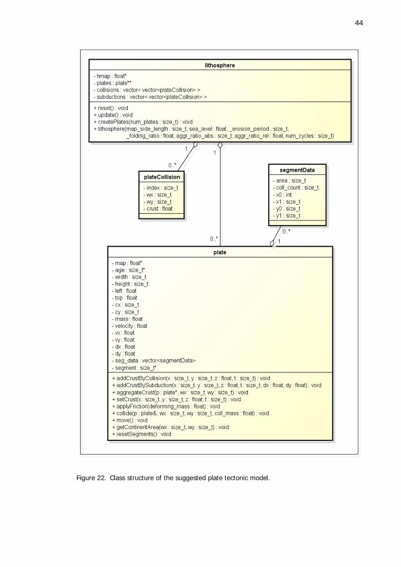
44

Figure 22. Class structure of the suggested plate tectonic model.

45

A plate is a two dimensional map, a rectangle grid, moving from some location at some

speed to some direction. The position of a plate is the location of its top-left corner on

the world map. A plate's speed is a non-negative scalar and its direction is a two di-

mensional unit vector. They are initialized with random values when the plate is creat-

ed. Because a plate's speed is a unit vector, all vector calculations that are done when

plates collide are simplified greatly. Lastly a plate contains a vector for storing the

changes to its speed and velocity since the plate last moved. This vector is not a unit

vector and thus the direction and speed must be extracted and updated separately

before the plate is moved again. However, applying external forces to a plate's trajec-

tory is simpler when one doesn't need to split the force vector into unit vector and

magnitude.

A plate contains complete information of the amount of crust at each location on it and

the characteristic age of crust at each location in two arrays, whose widths and heights

equal the dimensions of the plate along X and Y axis, respectively. This design was

chosen for its simplicity, increased realism and speed. Firstly, when oceanic plate sub-

ducts under another oceanic plate, islands emerge. When subduction has been going

on for some time, islands grow together and form a single giant island or a continent.

Should each plate contain only continental crust as was done in Cdrift, their bookkeep-

ing would become exceedingly cumbersome and inefficient as new plates would be

created for every tiny island and merged together when they finally grow on top of

each other. Secondly, real world tectonic plates contain both continental and oceanic

crust as is evident from Figure 14. Every single plate that contains continental crust

also contains some oceanic crust. When the direction of the continent changes due to

a collision or some other event, the islands that sit in the accompanied ocean change

their directions as well. Lastly, adding to and removing crust from arbitrary locations is

trivial with a rectangle bitmap as opposed to e.g. some sort of polygon presentation.

In addition to the information provided above, a plate also records its total mass and

the location of its center of mass as offset from the left-top corner into the plate. The-

se are updated when something changes in the plate's topography and they are used

in the plate collision routines. They could be re-calculated from scratch every time

they're needed, removing the need for additional member variables, but that'd be

simply a waste of processing time.

46

Lastly, a plate contains a resizable array of segment data objects. A segment data ob-

ject is the plate's internal, private class that contains the dimensions and surface area

of a single continent within that plate. A continent is defined as a group of adjacent

points that are all above sea level. Each continent within a plate is given their own

identification number. If some points of crust on the plate belong to a continent whose

identification number is ID, then its corresponding location in the identification bitmap

is marked with ID. The identification bitmap is an array just like the crust and age ar-

rays mentioned earlier.

Crust deformations on a plate can be performed by

adding crust on the plate when two plates collide. The parameters of the

receiving continent on the receiving plate are updated to reflect the defor-

mation.

initiating a subduction at some location on the plate. The exact location where

the subducted crust is added is at some distance into the overlying plate along

the trajectory of the subducting plate from the point of subduction. This simu-

lates the behavior described in chapter 4.2.1.

aggregating an entire continent from one plate to another. This simulates the

merging of two continents into one.

dictating directly the amount and age of crust at some location. These defor-

mations are done with addCrustByCollision, addCrustBySubduction,

aggregateCrust and setCrust, respectively.

Plate movement is controlled by

collide method, which updates the directions and velocities of two colliding

plates according to Newton's laws of motion.

applyFriction method, which slows the plate down some amount depend-

ing on the mass of plate: larger plates are less affected by the same amount of

friction than small plates.

47

move method, which updates plate's direction and velocity and then moves

plate.

The segmentation of a plate into separate continents is done internally by the methods

mentioned previously. The user of the class can force the plate to remove all segmen-

tation bookkeeping with resetSegments method. The surface area of a continent at

some location on the plate can be queried by getContinentArea method.

Lithosphere is the container and director of all the plates of the system. During each

call to update method it moves all plates, resolves collisions and updates the topogra-

phy and crustal age maps of the entire lithosphere to match that of the grand total of

all plates. However, from a structural point of view the most interesting part of the

class are the constructor parameters:

map_side_length determines the width and length of the square, two di-

mensional map that represents the entire lithosphere and thus the surface of

the planet.

sea_level is a hint of the amount of dry land in the initial setting before any

tectonic simulation has taken place. A value of 0.0 would result in a planet cov-

ered with water. Plate tectonics would bring forth islands that would later

merge into continents. A value of 1.0 would result in a lithosphere that's devoid

of any oceanic crust, being completely filled with continents. Such initial setting

would cause plate tectonics to halt at the very first steps.

_erosion_period determines the amount of iterations, i.e. the number of

consecutive calls to update method that should pass between sequential runs

of the erosion algorithm. A value of zero would mean that erosion is never ap-

plied to the system.

_folding_ratio is the amount of crust that is moved from the source plate

to the destination plate at the location where two plates overlap. A value of 0.0

would mean that nothing is transferred, 1.0 causes everything to be transferred

48

immediately. The destination plate is that which has a larger continent at the

location of collision.

aggr_ratio_abs is an abbreviation of "absolute aggregation ratio". In short

it defines the minimum amount of surface area that one continent on a plate

must overlap with another continent on another plate during that iteration be-

fore the two continents are merged into one continent that resides on either

plate. The smaller continent will always be merged to the larger one.

agg_ratio_rel defines the minimum percentage of surface area of a conti-

nent that must overlap with another continent before they are merged into one

continent. A value of 0.0 would cause two colliding continents to become

merged immediately. A value of 1.0 requires that the smaller plate is complete-

ly beneath the larger plate before they are merged together. This parameter is

in a central role when the rate of continental growth is adjusted.

num_cycles sets the maximum number of times that the lithosphere is divid-

ed into plates. If zero, then new set of plates are generated instead of the old

ones every time the sum of plate movement slows down too much.

These variables, along with the number of plates, control the behavior of the model

and affect its outcome greatly. Additionally they simplify the testing of the model a lot,

because the code does not need to be recompiled after one parameter is slightly ad-

justed. All parameters can be fed to the program as command line arguments.

When two plates overlap, the lithosphere records the location of the collision, the

plates involved in the collision and the amount of crust transferred in the collision in an

instance of plateCollision class. Collisions leading to subduction are saved in their own

list and continental collisions in their own. There are actually as many lists for both

subduction and continental collisions as lithosphere has plates. These lists are saved in

two arrays in the lithosphere class, respectively. This way the index of the other plate

participating in the collision is neatly determined by the index of the list it is stored to

in the array of lists.

49

This design has several other rationales too. First, when collision lists are class mem-

bers, their memory area can be reserved once and then simply recycled. This reduces

the time consumed by repeated freeing and reallocation of memory and reduces

memory fragmentation. Second, the code in the update method simplifies greatly when

all collisions are first recorded at one point and then processed at some different loca-

tion. Third, when all collisions to one plate are processed one after another, the range

of memory accesses narrows down and caching of code and data becomes more effi-

cient. Finally, organizing the collisions by type enables the processing of all subductions

first and all continental collisions then, which is important when subduction happens

under a plate that is simultaneously colliding to a bigger plate and would be aggregat-

ed to it and thus removed from the plate that is about to receive subducted material.

7.4 Program Behavior

The runtime behavior of the implementation consists of two main steps: initialization

and update cycle. Of these the initialization step will be discussed first. The program's

shutdown step is not treated in the text due to its extreme simplicity: all allocated re-

sources are simply freed and the program is closed.

Program initialization consists of setting up lithosphere according to the parameters

received from the user at startup and populating it with plates. Upon creation the litho-

sphere generates a fractal terrain onto the world map. The terrain consists of a nearly

flat ocean floor and continents. The amount of dry land is guided by the sea_level

parameter introduced earlier.

Plates are created on the lithosphere by selecting randomly and uniformly the desired

amount of locations where a plate will emerge. A plate is formed around such location

in the following manner: Select a random point adjacent to any point of this plate. If

that point doesn't belong to any plate yet, attach it to this plate. When this is done to

each plate in parallel, plate patterns like those seen in Figure 23 emerge.

50

Figure 23. Lithosphere divided into plates. Different colors denote different plates and have nothing to do with topography.

After the plate has been formed, it is created and added to the lithosphere's list of

plates. Upon initialization each plate assigns to itself a random direction and random

velocity. Finally the main loop may begin with the first call to the lithosphere's update

method.

The update method in the lithosphere class begins by checking whether the amount of

action across plates is enough to continue with the current set of plates. If plates have

slowed down too much and too few collisions are happening, the set of plates is re-

populated: old plates are discarded and replaced by new plates like described earlier.

This ensures that the simulation doesn't get stuck or take too much time to create in-

teresting topographies.

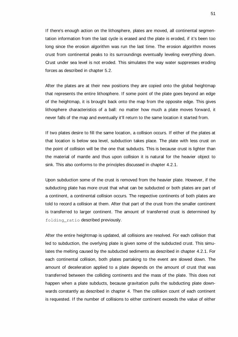
51

If there's enough action on the lithosphere, plates are moved, all continental segmen-

tation information from the last cycle is erased and the plate is eroded, if it’s been too

long since the erosion algorithm was run the last time. The erosion algorithm moves

crust from continental peaks to its surroundings eventually leveling everything down.

Crust under sea level is not eroded. This simulates the way water suppresses eroding

forces as described in chapter 5.2.

After the plates are at their new positions they are copied onto the global heightmap

that represents the entire lithosphere. If some point of the plate goes beyond an edge

of the heightmap, it is brought back onto the map from the opposite edge. This gives

lithosphere characteristics of a ball: no matter how much a plate moves forward, it

never falls of the map and eventually it'll return to the same location it started from.

If two plates desire to fill the same location, a collision occurs. If either of the plates at

that location is below sea level, subduction takes place. The plate with less crust on

the point of collision will be the one that subducts. This is because crust is lighter than

the material of mantle and thus upon collision it is natural for the heavier object to

sink. This also conforms to the principles discussed in chapter 4.2.1.

Upon subduction some of the crust is removed from the heavier plate. However, if the

subducting plate has more crust that what can be subducted or both plates are part of

a continent, a continental collision occurs. The respective continents of both plates are

told to record a collision at them. After that part of the crust from the smaller continent

is transferred to larger continent. The amount of transferred crust is determined by

folding_ratio described previously.

After the entire heightmap is updated, all collisions are resolved. For each collision that

led to subduction, the overlying plate is given some of the subducted crust. This simu-

lates the melting caused by the subducted sediments as described in chapter 4.2.1. For

each continental collision, both plates partaking to the event are slowed down. The

amount of deceleration applied to a plate depends on the amount of crust that was

transferred between the colliding continents and the mass of the plate. This does not

happen when a plate subducts, because gravitation pulls the subducting plate down-

wards constantly as described in chapter 4. Then the collision count of each continent

is requested. If the number of collisions to either continent exceeds the value of either

52

of the threshold parameters described in the previous chapter, the plate that is smaller

in surface area is merged to the larger plate. Upon merging, the plate containing the

joint continent is given a new direction according to Newton's laws of motion. Thus a

small island colliding to a giant continent affects its trajectory only slightly, and vice

versa.

The way plate collisions are counted leaves much room for improvement. A large plate

might receive simultaneously many collisions from several distinct continents, but be-

cause all collisions are summed up into one number, the small continents become

merged to the large continent much more easily, resulting in a giant continent far

sooner than the user might have desired. To overcome this problem there are two ag-

gregation threshold parameters: the artifact just mentioned can be avoided by setting

the threshold of the number of collisions compared to the continent's area to some

appropriate value. However, this relative overlap parameter alone would at worst

cause very large continents to slide by each other forever without merging. Balancing

these two parameters is a delicate subject, for it has a remarkable effect on the result

of the simulation.

After all collisions are processed, those locations on the lithosphere that have no crust

are filled with new oceanic crust. The crust is attached to the plate that was located

there during the previous iteration. This simulates the mechanisms described in chap-

ter 4.1. Finally, a delicate visual effect is added to the oceanic crust: younger and thus

more buoyant crust is lifted up on the global heightmap. This helps to visualize ocean

ridges without complicating the way plate collisions are managed. After the update is

done, the resulting heightmap is drawn on the screen for the user to see.

53

8 Results

8.1 Topographical Features

The straightforward implementation of the greatly simplified model of plate tectonics

that was introduced and described in the previous chapters is capable of producing a

rather broad variety of land forms seen in the nature. The resulting topographic maps

(Figure 24) contain thin mountain ranges that run across continents, sharp coastal

mountain ranges resulting from the subduction of oceanic crust, wide mountainous

areas like the Himalayas and vast plains. Islands of various shapes, sizes and for-

mations arise from the seas: some islands remain in solitude, others form clusters or

chains.

Figure 24. Output from the implemented terrain generator. The labeled landforms are A) mountain range between colliding continents, B) coastal mountain belt, C) large island and D) island chain.

54

However, many types of topography that is found from the nature is still missing from

the simulation's output. Seafloors have no ocean trenches and ridges are not visible at

the boundary of two spreading plates. Likewise continents are missing trenches or

steep valleys such as the surroundings of Saint Lawrence River in Canada or Lake Tan-

ganyika in East Africa. Lastly, the maps the generator produces are completely missing

continental shelves, the flat extensions of continents covered by relatively shallow

seas. These shelves and all other natural topographic features are shown in Figure 25

(appendix 1).

The generated maps contain artifacts that are easy to spot. Firstly, seafloors are un-

naturally smooth. This is due to leaving out of hot spots and transformation faults and

poor rendering of ocean ridges and trenches. Secondly, the resulting shorelines lack

the jaggedness found in natural and fractal shores. The same observation can be made

of the mountain ranges and practically the entire continental topography which is ex-

ceedingly smooth when compared to the rugged and detailed texture of natural conti-

nents and mountain ranges. These flaws are due to the type of erosion algorithm used,

which actually is not an erosion algorithm at all but a modified blurring algorithm.

The parameters that control the behavior of lithosphere have a substantial effect on

the credibility of the generator's output. For example, if the required amount of relative

and absolute overlap is too small, continents will attach to each other quickly resulting

in thin mountain ranges; the same effect is exhibited if the amount of crust that will

fold when continents collide is too large. If there are too many plates or too many cy-

cles, the continents become small and scattered resulting in a map with many small

islands. Finding the range of optimal values for all the parameters requires lots of

manual experimenting and is more of an art than a science. In order to save the trou-

ble from users of the generator, parameters have been given default values that are

most likely to produce realistic results.

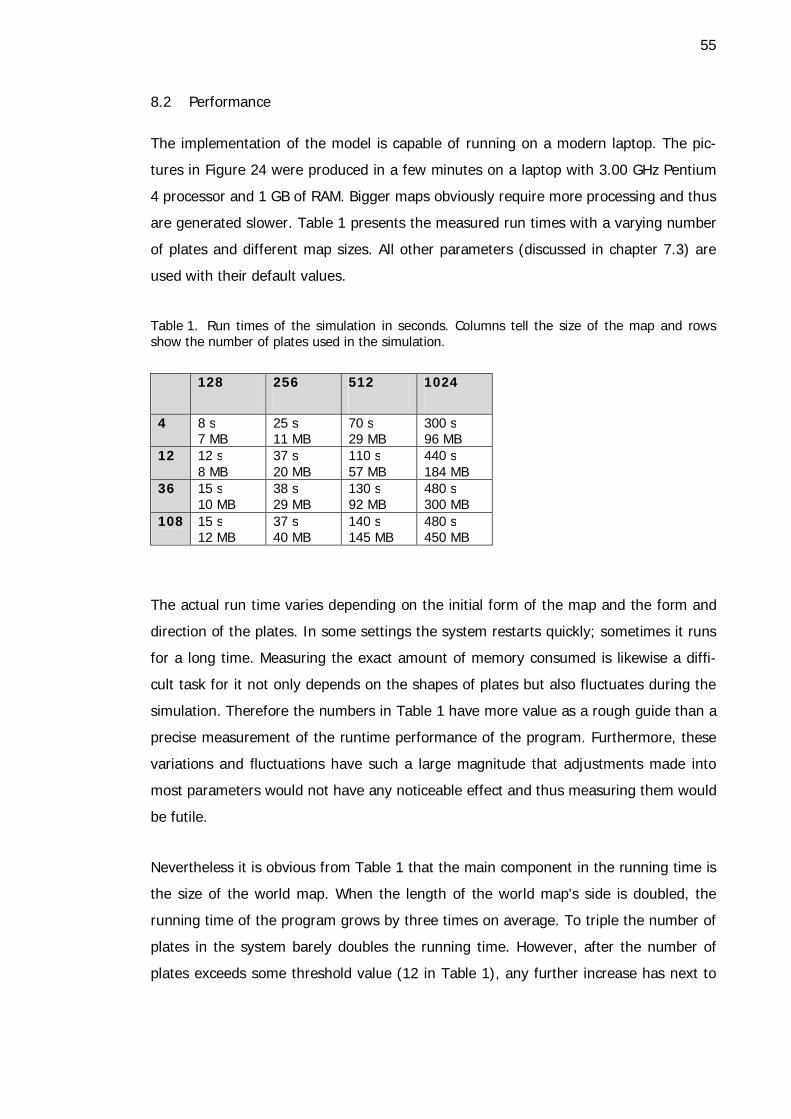
55

8.2 Performance

The implementation of the model is capable of running on a modern laptop. The pic-

tures in Figure 24 were produced in a few minutes on a laptop with 3.00 GHz Pentium

4 processor and 1 GB of RAM. Bigger maps obviously require more processing and thus

are generated slower. Table 1 presents the measured run times with a varying number

of plates and different map sizes. All other parameters (discussed in chapter 7.3) are

used with their default values.

Table 1. Run times of the simulation in seconds. Columns tell the size of the map and rows show the number of plates used in the simulation.

128 256 512 1024

4 8 s 7 MB

25 s 11 MB

70 s 29 MB

300 s 96 MB

12 12 s 8 MB

37 s 20 MB

110 s 57 MB

440 s 184 MB

36 15 s 10 MB

38 s 29 MB

130 s 92 MB

480 s 300 MB

108 15 s 12 MB

37 s 40 MB

140 s 145 MB

480 s 450 MB

The actual run time varies depending on the initial form of the map and the form and

direction of the plates. In some settings the system restarts quickly; sometimes it runs

for a long time. Measuring the exact amount of memory consumed is likewise a diffi-

cult task for it not only depends on the shapes of plates but also fluctuates during the

simulation. Therefore the numbers in Table 1 have more value as a rough guide than a

precise measurement of the runtime performance of the program. Furthermore, these

variations and fluctuations have such a large magnitude that adjustments made into

most parameters would not have any noticeable effect and thus measuring them would

be futile.

Nevertheless it is obvious from Table 1 that the main component in the running time is

the size of the world map. When the length of the world map's side is doubled, the

running time of the program grows by three times on average. To triple the number of

plates in the system barely doubles the running time. However, after the number of

plates exceeds some threshold value (12 in Table 1), any further increase has next to

56

no effect on the performance. This is because some plates tend to grow in the surface

area during the simulation, leaving less room for other plates. Eventually they become

so large that they alone cover the entire lithosphere, causing the rest of the plates to

become empty and thus have no contribution to the simulation whatsoever.

The size of the lithosphere dominates also the amount of memory. Increasing the

number of plates nine times is roughly equal to doubling the size of the lithosphere,

memory-wise. However, the larger the lithosphere, the larger effect the increase in the

number of plates has on memory consumption. This is only natural, for as explained in

chapter 7.3, each plate is a rectangle map that contains the plate's entire topography.

When plates grow e.g. diagonally, the memory they consume is far greater than their

surface area on the lithosphere. Thus the few plates that cover the entire lithosphere

consume many times the amount of memory of the lithosphere itself.

The run time results are encouraging. With a moderate increase in algorithmic com-

plexity the running time could maybe be cut into half or less. Such optimizations might

include removal of nearly empty plates, caching of collision statistics of plates between

iterations, processing all collisions between two plates as a single collision bundle and

more effective segmentation algorithm.

57

9 Future Work

As is evident from chapter 7.2, the model introduced in the preceding chapters con-

tains many very significant simplifications which not only causes some natural land-

forms to be missing from the output but is also the source of some notable artifacts, as

described in chapter 8.1. Maybe the most apparent place for improvement is the im-

plementation of a proper erosion algorithm that would simulate the processes found in

nature described in chapter 5.2. This would lead to more natural mountain ranges and

continental texture overall. Another, very obvious improvement is the inclusion of re-

jected features such as hot spots, ocean ridges and trenches and maybe even back-arc

basins.

In the current implementation all plates move along a straight line. Sometimes this

creates quite obvious artifacts, for example a long line like islands. This flaw could be

avoided and maybe many new topographic details might emerge if plates had angular

velocity in addition to directional velocity.

Another rather trivial improvement would be to give each plate their own, personalized

copy of the set of parameters that are currently given to the entire lithosphere and

applied to all plates equally (see chapter 7.3). This would certainly increase the diversi-

ty of types of details in the heightmap and thus make the output of the simulation

much more interesting. Finally, the performance of the simulation could be boosted

considerably as discussed in the previous chapter.

However, at the heart of all artifacts and missing landforms exhibited by the simulation

presented in this paper is the lack of physical accuracy in the modeling of all types of

convergent plate boundaries. While this is rather obvious, the solution that fixes the

problem and still runs on a personal computer is far from it. When plates are modeled

as square grids with fixed sized elements, some very creative workarounds that can be

hard to implement are needed to correctly simulate the folding and displacement of

the crust. A far more flexible and intuitive approach would be to use three dimensional

polygon mesh or point-sample based model like done in [31]. Such an approach would

allow the modeling of a plate as a group of individual pieces of crust whose position

relative to the other pieces in the plate is not fixed. This would enable a far more phys-

ically accurate simulation of the strains and stresses that plates cause in each other.

58

For example, the folding of a continent would cause the pieces of crust at the colliding

edge of the plate to draw nearer to each other and simultaneously grow in height in

order to keep the thickness of the crust constant, just as described in chapter 4.2.2.

Likewise, an edge of a continent pulled by a subducting oceanic lithosphere would

cause the pieces of crust at the weakest point of the continent to draw away from each

other eventually resulting in the detachment of the edge of the continent and thus in

the formation of a back-arc basin, just as described in chapter 4.2.1.

As mentioned in the previous chapter, the seafloors are unnaturally even in the current

implementation, for it is unable to produce transformation faults. In a flat two dimen-

sional world it is undoubtedly difficult to produce realistic transformation faults like

those seen in appendix 1. This is because movement on a flat surface differs radically

from movement on a sphere. For example, consider a plate on a sphere: suppose all

the points of the plate have constant speed on the surface of the sphere and they're

moving west along the equator. Therefore the points of the plate far away from the

equator would have gone around full circle before those at the equator, because the

circumference of a sphere at the equator is longer than near the poles. Thus the plate

becomes fragmented into several horizontal stripes that have transformation faults

between them. Accordingly, when the model is taken from the two dimensional Carte-

sian coordinate system to the three dimensional polar coordinate system, new forces

that naturally stem from the spherical geometry of the lithosphere will be introduced

into the model as illustrated above. This results in much more realistic sea floor fault-

ing and continental interaction.

However, adding a new dimension to the simulation will take its toll on the complexity

and performance of the program. Combined with the greatly increased level of detail in

the modeling of a plate and substantially elevated amount of computation required to

solve the interactions between every point of each plate at a single time step, it might

become simply impossible to run the simulation on a personal computer at any sort of

acceptable rate.

59

10 Conclusions

This thesis explores the use of the theory of plate tectonics in procedural terrain gen-

eration. A simple computer implementation that mimics the plate tectonic processes

observed on the Earth was built for demonstrating the issues that surface when the

theory is put into practice. Together with the theoretical overview of plate tectonics

presented in this thesis they serve as a thorough introduction for hobbyist game pro-

grammers or as a starting point for more serious future work.

The overall quality of the heightmaps from the greatly simplified plate tectonic simula-

tor far exceeds the amount of realism found in terrains produced by typical fractal

methods. Mountain ranges of varying size and shape emerge between colliding conti-

nental plates. Subduction of oceanic crust under a continent produces coastal moun-

tain ranges. Between mountains and highlands there are vast flat areas just like in the

world around us. Island chains are born where two oceanic plates collide and new

crust is created to fill the gap between the diverging plates. Upon collision islands

merge together and become larger and larger. All of these are features that conven-

tional fractal terrains are missing.

Nevertheless, the simplifications made into the implemented model caused some fea-

tures to be missing and some unpleasant visual artifacts to occur. The most notable is

the lack of detail in the produced maps. This is especially easy to see in ocean floors

that are practically completely flat. There are also no continental shelves like those

surrounding the continents on the Earth. Hot spots are not simulated at all. Lastly,

mountain ranges are missing all the roughness that governs the appearance of real

world mountains. This is mostly due to a far too simple erosion algorithm. Additionally,

mountain ranges sometimes end up having rather peculiar shape due to the way con-

tinents are melt together in the simulation.

To overcome these shortcomings, more detail and physical accuracy should be incorpo-

rated into the implementation. The plates could be modeled point by point instead of

treating them as one big lump of crust. This would enable realistic merging and tearing

apart of plates. Erosion could be made to simulate the way water alters landforms on

the Earth. Subduction could take gravity and the density of the subducting crust into

60

account allowing credible formation of back-arc basins. Finally, the entire simulation

could be taken from the flat two dimensional surface onto a three dimensional sphere.

All in all it seems safe to say that the simulation of plate tectonics will have an increas-

ing amount of importance in the game and movie industries in the future. Fractal

methods require lots of post processing and there is still no guarantee that they can

produce realistic maps. Anything is possible when terrain is created manually, but that

is slow and expensive when compared to using computers to generate content. It is

therefore crucial to continue developing physically based terrain generation techniques

with the goal of producing very realistic artificial heightmaps on a typical workstation in

a matter of minutes.

61

References

[1] Persson, Markus. 2011. Terrain generation, Part 1. Online document. <http://notch.tumblr.com/post/3746989361/terrain-generation-part-1>. Updated 9.3.2011. Accessed 18.3.2012. [2] Terragen 2 in Sucker Punch. 2009. Online Document. Planetside Software. <http://www.planetside.co.uk/content/view/64/100/> Accessed 18.3.2012. [3] Terragen™ 2. 2009. Online Document. Planetside Software. <http://www.planetside.co.uk/content/view/15/27/> Accessed 18.3.2012. [4] Artificial Terrain Generation. 2008. Online Document. The Virtual Terrain Project. <http://vterrain.org/Elevation/Artificial/> Updated 14.3.2012. Accessed 18.3.2012. [5] Feder, Jens. 1988. Fractals. New York: Plenum Press. [6] Koch curve (L-system construction).jpg. 2005. Online Document. Wikimedia Com-mons. <http://commons.wikimedia.org/wiki/File:Koch_curve_%28L-system_construction%29.jpg> Updated 5.4.2011. Accessed 18.3.2012. [7] Self similarity in the Mandelbrot set. 2005. Online Document. Wikimedia Commons. <http://commons.wikimedia.org/wiki/File:Mandelbrot-similar1.png> <http://commons.wikimedia.org/wiki/File:Mandelbrot-similar2.png> <http://commons.wikimedia.org/wiki/File:Mandelbrot-similar3.png> <http://commons.wikimedia.org/wiki/File:Mandelbrot-similar4.png> Updated 21.8.2009. Accessed 18.3.2012. [8] Paul Martz. 1997. Generating Random Fractal Terrain. Online Document. Game Programmer. <http://gameprogrammer.com/fractal.html> Accessed 18.3.2012. [9] Miller, Russell. 1983. Planet Earth, Continents In Collision. Amsterdam: Time-Life Books. [10] Schubert, G., Turcotte, D. L. & Olson, P. 2001. Mantle Convections in the Earth and Planets. United Kingdom: Cambridge University Press. [11] Earth internal structure. 2011. Online Document. Wikimedia Commons. <http://commons.wikimedia.org/wiki/File:Earth_internal_structure.png> Updated 3.11.2011. Accessed 18.3.2012. [12] Sawkins, F. J., Chase, C. G., Darby, D. G. & Rapp, G., Jr. 1978. The Evolving Earth: a Text in Physical Geology, 2nd Edition. New York: Macmillian Publishing Co., Inc. [13] Turcotte, D. L. & Schubert, G. 2002. Geodynamics, 2nd ed. United Kingdom: Cambridge University Press.

62

[14] "Hannes Grobe". 2007. Stages of the Wilson-Cycle. Online Document. Wikimedia Commons. <http://commons.wikimedia.org/wiki/File:Wilson-stages_hg.png> Updated 25.12.2010. Accessed 18.3.2012. [15] Tasa, Dennis. 2012. Tasa Graphic Arts, Inc. Private communication 22.2.2012. [16] "Mikenorton". 2007. Diagram to explain processes associated with subduction. Online Document. Wikimedia Commons. <http://en.wikipedia.org/wiki/File:Subduction01.jpg> Updated 28.11.2007. Accessed 18.3.2012. [17] Beardsmore, G. R. & Cull, J. P. 2007 Crustal Heath Flow, a guide to Measurement and Modelling. United Kingdom: Cambridge University Press. [18] "Gregors". 2011. Types of geologic faults. Online Document. Wikimedia Com-mons. <http://commons.wikimedia.org/wiki/File:Types_of_Faults.svg> Updated 1.3.2011. Accessed 18.3.2012. [19] Šubelj, Gašper. 2006. A scheme showing the syncline and anticline. Online Docu-ment. Wikimedia Commons. <http://commons.wikimedia.org/wiki/File:Syncline_and_anticline.jpg> Updated 14.3.2006. Accessed 18.3.2012. [20] News Release : Earth's Moving Crust May Occasionally Stop. 2008. Online Docu-ment. Woods Hole Oceanographic Institution. <http://www.whoi.edu/page.do?pid=39137&tid=282&cid=35767&ct=162> Updated 14.03.2012. Accessed 18.03.2012. [21] Transform fault. 2008. Online Document. Wikimedia Commons. <http://commons.wikimedia.org/wiki/File:Transform_fault-1.svg> Updated 18.11.2010. Accessed 18.3.2012. [22] The Romanche Trench. 2006. Online Document. Wikimedia Commons. <http://commons.wikimedia.org/wiki/File:Romanche_Trench.jpg> Updated 29.9.2009. Accessed 18.3.2012. [23] World map in English of selected prominent geological hotspots. 2006. Online Document. Wikimedia Commons. <http://commons.wikimedia.org/wiki/File:Tectonic_plates_hotspots-en.svg> Updated 14.1.2011. Accessed 18.3.2012. [24] Map of the Hawaii-Emperor seamount chain and seafloor topography. 2008. Online Document. Wikimedia Commons. <http://commons.wikimedia.org/wiki/File:Hawaii-Emperor_engl.png> Updated 25.10.2010. Accessed 18.3.2012. [25] Erickson, Jon. 2001. Plate Tectonics, Unraveling the Mysteries of the Earth (The Living Earth) (Revised Edition). New York: Checkmark books. [26] Monsoons are spinning the Earth’s plates. 2011. Online Document. Cosmos Maga-zine. Updated 13.4.2011. Accessed 18.3.2012.

63

[27] "MesserWoland". 2007. Isostatic (Airy) equilibrium of the Earth's crust. Online Document. Wikimedia Commons. <http://commons.wikimedia.org/wiki/File:Isostasy.svg> Updated 9.4.2007. Accessed 18.3.2012. [28] "Impaler[WrG]". 2003. Map Generation and Rivers. Online Document. The Apoly-ton Civilization Site. <http://apolyton.net/showthread.php/80438-Map-Generation-and-Rivers?s=9414da78dd86d4da6b29846a607b113c> Updated 28.3.2003. Accessed 18.3.2012. [29] "Impaler[WrG]". 2011. User of the Apolyton Civilization Site. Private Communica-tion 5.7.2011. [30] Allen, David. 1991. cdrift. Online Document. World Builder Page - Landscape Utili-ties. <http://markjstock.org/pages/builder.html> Updated 27.1.2006. Accessed 18.3.2012. [31] Jarocha-Ernst, Alex. 2006.Creating Landscapes with Simulated Colliding Plates. Master's Thesis. Rochester Institute of Technology, Department of Computer Science. [32] Svitil, Kathy. 2010. New View of Tectonic Plates. Online Document. California In-stitute of Technology. <http://media.caltech.edu/press_releases/13375> Updated 25.8.2010. Accessed 18.3.2012. [33] Stadler, G., Gurnis, M., Burstedde, C., Wilcox, L. C., Alisic, L. & Ghattas O. 2010. The Dynamics of Plate Tectonics and Mantle Flow: From Local to Global Scales. Science Magazine, vol. 329, pp. 1034-1037. [34] Global land and undersea elevation. 2006. Online Document. Wikimedia Com-mons. <http://en.wikipedia.org/wiki/File:Elevation.jpg> Updated 7.3.2006. Accessed 18.3.2012.

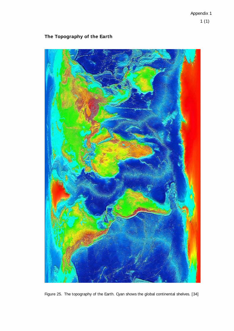
Appendix 1

1 (1)

The Topography of the Earth

Figure 25. The topography of the Earth. Cyan shows the global continental shelves. [34]