Physically based modelling of sediment generation and transport under a large rainfall simulator

HYDROLOGICAL PROCESSESHydrol. Process. 20, 2253–2270 (2006)Published online 20 March 2006 in Wiley InterScience (www.interscience.wiley.com). DOI: 10.1002/hyp.6050

Physically based modelling of sediment generation andtransport under a large rainfall simulator

Russell Adams1* and Sandy Elliott2

1 Department of Civil and Environmental Engineering, University of Massachusetts, 18 Marston Hall, Amherst, MA 01003, USA2 National Institute of Water and Atmospheric Research Ltd, PO Box 11-115, Hamilton, New Zealand

Abstract:

A series of large rainfall simulator experiments was conducted in 2002 and 2003 on a small plot located in anexperimental catchment in the North Island of New Zealand. These experiments measured both runoff and sedimenttransport under carefully controlled conditions. A physically based hydrological modelling system (SHETRAN) wasthen applied to reproduce the observed hydrographs and sedigraphs. SHETRAN uses physically based equations torepresent flow and sediment transport, and two erodibility coefficients to model detachment of soil particles by raindroperosion and overland flow erosion. The rate of raindrop erosion also depended on the amount of bare ground underthe simulator; this was estimated before each experiment. These erodibility coefficients were calibrated systematicallyfor summer and winter experiments separately, and lower values were obtained for the summer experiments. Earlierstudies using small rainfall simulators in the vicinity of the plot also found the soil to be less erodible in summer andautumn. Limited validation of model parameters was carried out using results from a series of autumn experiments.The modelled suspended sediment load was also sensitive to parameters controlling the generation of runoff fromthe rainfall simulator plot; therefore, we found that accurate runoff predictions were important for the sedimentpredictions, especially from the experiments where the pasture cover was good and overland flow erosion was thedominant mechanism. The rainfall simulator experiments showed that the mass of suspended sediment increased post-grazing, and according to the model this was due to raindrop detachment. The results indicated that grazing cattle orsheep on steeply sloping hill-country paddocks should be carefully managed, especially in winter, to limit the transportof suspended sediment into watercourses. Copyright 2006 John Wiley & Sons, Ltd.

KEY WORDS rainfall simulator; physically based modelling; erosion modelling; sediment transport; raindropdetachment; shear entrainment

INTRODUCTION

Grazing by sheep or beef cattle in the New Zealand hill country is an established agricultural industry and is adominant land use in many areas of the country. Associated with this industry is the generation of sediment byhillslope erosion, especially if land management practices are poor (Lambert et al., 1985; Harrod and Theurer,2003). Specific impacts from the increased sediment loads attributed to the damage to pasture by livestockinclude decreased soil fertility, the transport of particulate nutrients to waterways and detrimental effects uponaquatic and estuarine biota. In the North Island hill country the problem is acute due to steep slopes, erodiblesoils and a seasonally high rainfall, including short-duration events of high intensity. Additionally, livestockusually graze the pasture catchments intensively without a seasonal break, damaging the soil and generatingsediment. There is a trend towards intensive winter grazing of cattle on steep pasture (Elliott et al., 2002). Thestocking rates are often high and damage by poaching (treading of the surface of moist or saturated soil) takesplace even if the grazing lasts for only 2–3 days (Nguyen et al., 1998). Further damage may be generatedby animal and machinery traffic (Harrod and Theurer, 2003). After grazing by sheep, McColl and Gibson

* Correspondence to: Russell Adams, Department of Civil and Environmental Engineering, University of Massachusetts, 224 Marston Hall,Amherst, MA 01003-5205, USA. E-mail: [email protected]

Received 30 June 2004Copyright 2006 John Wiley & Sons, Ltd. Accepted 12 May 2005

2254 R. ADAMS AND S. ELLIOT

(1979) found that concentrations of suspended sediment (SS) and nutrients (excepting nitrate) in overlandflow increased immediately then declined in subsequent events. Elliott et al. (2002) found that the effects ofcattle grazing were longer lasting. Two months after grazing, the area of bare ground was reduced to half theoriginal area on average, the exact rate of recovery varying by soil type.

This paper describes a study of the runoff and erosion processes controlling sediment transport, using acombination of field-scale large rainfall simulator experiments and hydrological modelling. Rainfall simulatorsare useful because the duration and intensity of the applied rainfall can be carefully controlled and thesimulations can link into an intensive monitoring campaign (Bowyer-Bower and Burt, 1989). In New Zealand,small simulators of the order of 0Ð5 m2 in area have been used to study the impacts of cattle grazing (Campbell,1945; Selby, 1972; Nguyen et al., 1998; Elliott et al., 2002) and sheep grazing (Elliott and Carlson, 2004)on erosion and infiltration. However, these experiments only simulate small-scale erosion processes, mainlyraindrop detachment of soil particles, and the plots are not large enough for significant surface runoff pathwaysto develop. Large rainfall simulators can simulate both raindrop erosion and the development of rill and sheeterosion, since longer overland flow pathways can develop naturally on the hillslope during the experiment.Large rainfall simulators have been applied worldwide to study erosion processes on a larger scale. Forexample Lane et al. (2004) used two 300 and 450 m2 rainfall simulators to study runoff processes in loggedand burnt eucalyptus forests in Australia.

Small rainfall simulator experiments carried out on plots in the vicinity of the experimental site describedin this paper showed that grazing by cattle resulted in patches of bare soil, which in turn increased the SSload. In winter, Nguyen et al. (1998) found that grazing also compacted the ground, reducing the infiltrationcapacity of the soil and leading to an increase in both runoff and SS load. The effects of intensive cattlegrazing in winter (Elliott et al., 2002) included a reduction by 50% of the infiltration capacity by treadingcompared with undamaged plots. The measured infiltration capacity in summer was approximately doublethe winter value. Elliott and Carlson (2004) also compared the effects of sheep grazing in summer and inwinter using both small and large rainfall simulators. The most extreme case (grazing in winter) increased SSconcentrations after grazing by a factor of 13–16. The soil erodibility varied seasonally, and in summer theSS concentrations were 2Ð5 times less than in winter. These experiments also identified a seasonal variationin infiltration capacity (November mean nearly twice the July mean).

One of the principal aims of the study was to show that hydrological modelling of flow and erosion in thelarge rainfall simulator plot could reproduce the observed SS loads at different times of the year and alsobefore and after grazing episodes. The SHETRAN hydrological modelling system (Ewen et al. 2000, 2002)was used, since it can simulate sediment erosion and transport processes, the governing equations for flowand transport have a physical basis, and the deterministic parameters can be based on field measurementswithout extensive model calibration.

This paper aims to show that the erodibility coefficients, used by SHETRAN to control the predicted amountof erosion, vary seasonally. It is hypothesized that the main reason for the increased SS concentrations andloads post-grazing is an increase in the amount of bare ground in the paddock created by stock trampling theground and grazing vegetation. The runoff generation mechanisms operating in the large rainfall simulatorplot and the modelling of runoff using SHETRAN have been presented in a companion paper (Adams et al.,2005).

THE SHETRAN MODELLING SYSTEM

SHETRAN (Ewen et al. 2000, 2002) is an updated version of the SHE physically based modelling system(Abbott et al., 1986), which can simulate transient three-dimensional flow, sediment and contaminant transportin catchments ranging from the plot scale to 5000 km2. SHETRAN is built around individual components(for simulating sediment transport for example), all of which share a common three-dimensional, grid-basedmesh structure. SHETRAN simulates three-dimensional water flow and two-dimensional sediment erosion and

Copyright 2006 John Wiley & Sons, Ltd. Hydrol. Process. 20, 2253–2270 (2006)

MODELLING OF SEDIMENT GENERATION AND RUNOFF 2255

transport using finite-difference approximations to the governing partial differential equations. At the groundsurface the model simulates both sheet overland flow (distributed across the entire surface area of a gridelement) and channel flow (which is simulated using channel elements orientated along the edges of the gridelements) using a component known as the OC (overland and channel flow) component. The latest versionof SHETRAN (V4.2 running on a PC) was used in this study.

We will now describe the sediment and erosion component of the model in more detail, as sediment isthe focus of this paper. The reader is referred to the above-mentioned references for descriptions of thehydrological components.

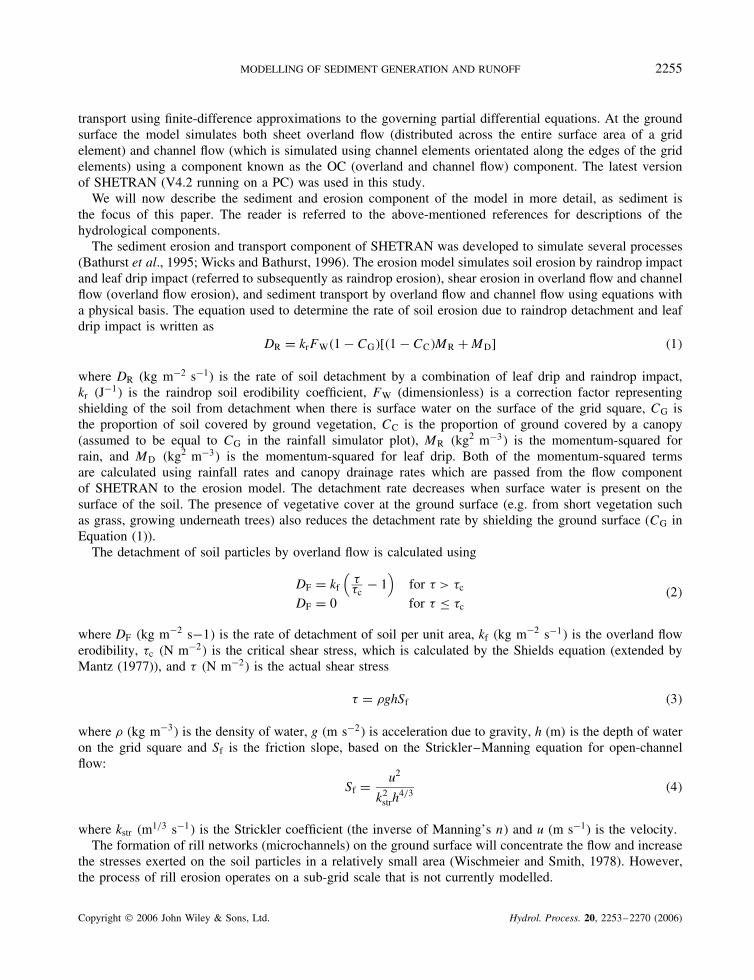
The sediment erosion and transport component of SHETRAN was developed to simulate several processes(Bathurst et al., 1995; Wicks and Bathurst, 1996). The erosion model simulates soil erosion by raindrop impactand leaf drip impact (referred to subsequently as raindrop erosion), shear erosion in overland flow and channelflow (overland flow erosion), and sediment transport by overland flow and channel flow using equations witha physical basis. The equation used to determine the rate of soil erosion due to raindrop detachment and leafdrip impact is written as

DR D krFW�1 � CG�[�1 � CC�MR C MD] �1�

where DR (kg m�2 s�1) is the rate of soil detachment by a combination of leaf drip and raindrop impact,kr �J�1� is the raindrop soil erodibility coefficient, FW (dimensionless) is a correction factor representingshielding of the soil from detachment when there is surface water on the surface of the grid square, CG isthe proportion of soil covered by ground vegetation, CC is the proportion of ground covered by a canopy(assumed to be equal to CG in the rainfall simulator plot), MR �kg2 m�3� is the momentum-squared forrain, and MD �kg2 m�3� is the momentum-squared for leaf drip. Both of the momentum-squared termsare calculated using rainfall rates and canopy drainage rates which are passed from the flow componentof SHETRAN to the erosion model. The detachment rate decreases when surface water is present on thesurface of the soil. The presence of vegetative cover at the ground surface (e.g. from short vegetation suchas grass, growing underneath trees) also reduces the detachment rate by shielding the ground surface (CG inEquation (1)).

The detachment of soil particles by overland flow is calculated using

DF D kf

(��c

� 1)

for � > �c

DF D 0 for � � �c�2�

where DF �kg m�2 s�1� is the rate of detachment of soil per unit area, kf �kg m�2 s�1� is the overland flowerodibility, �c �N m�2� is the critical shear stress, which is calculated by the Shields equation (extended byMantz (1977)), and � �N m�2� is the actual shear stress

� D �ghSf �3�

where � �kg m�3� is the density of water, g �m s�2� is acceleration due to gravity, h (m) is the depth of wateron the grid square and Sf is the friction slope, based on the Strickler–Manning equation for open-channelflow:

Sf D u2

k2strh

4/3 �4�

where kstr �m1/3 s�1� is the Strickler coefficient (the inverse of Manning’s n) and u (m s�1) is the velocity.The formation of rill networks (microchannels) on the ground surface will concentrate the flow and increase

the stresses exerted on the soil particles in a relatively small area (Wischmeier and Smith, 1978). However,the process of rill erosion operates on a sub-grid scale that is not currently modelled.



Transport of the eroded material by overland flow is calculated in SHETRAN using numerical solutions ofthe two-dimensional physically based conservative transport equation (after Wicks and Bathurst, 1996):

∂�hc�

∂tC �1 � ��

∂z

∂tC ∂gx

∂xC ∂gy

∂yD 0 �5�

where c �m3 m�3� is the sediment concentration, � is the soil surface porosity, z (m) is the depth of loose soil,t (s) is time, gx and gy �m3 s�1 m�1� are the sediment transport rates in the x and y directions respectively,and other terms were introduced above. Providing that there is sufficient transport capacity to carry theSS load entering the grid square from upstream, erosion by shear detachment can continue to take placeat each grid element. When the transport capacity of the flow has been reached, deposition of materialthen commences immediately and the excess material forms loose sediment. Transport capacity is calculatedusing the approach developed by Yalin (1963) for open channel flow, which has been used subsequentlyfor overland flow. Estimates of the values of the erodibility coefficients are generally made through modelcalibration (Wicks et al., 1992; Wicks and Bathurst, 1996).

METHODS

Rainfall simulator experiments

The large rainfall simulator plot is located in the 3 ha Pukemanga subcatchment, which drains into theMangaotama stream in the Whatawhata Research Centre (Figure 1). The Whatawhata Research Centre issituated 20 km west of Hamilton in the western North Island of New Zealand. The mean slope of the plot is18° and the area draining into the outlet was calculated from a detailed topographic survey to be approximately970 m2. The outlet itself drains directly into an ephemeral headwater stream (Pukemanga), which drains intothe Mangaotama stream about 100 m distant. The survey was used to create a grid-based digital elevationmodel (DEM) of the hillslope with a spatial resolution of 0Ð5 m. The large simulator has 13 rainfall standsat 9 m spacing (Figure 1). Each stand consists of a 5 m high pole with four closely spaced upward-sprayingsprinklers mounted on a frame at the top. Elliott and Carlson (2004) describe the background, experimentaldesign and operation of the large simulator in detail. The total application area under the sprinkler stands isgreater than the catchment area of the plot (approximately 1050 m2), since some of the rainfall falls outsidethe catchment boundary. The ground cover in the plot comprises dense rye grass and clover pasture that hasbeen grazed rotationally by both cattle and sheep. Surface runoff was measured at the downstream outlet ofthe plot using a flume connected to a data logger.

Soils in the plot have recently been investigated with a series of four soil pits (Muller et al., 2004) andgenerally consist of a silt loam Ap horizon overlying a Bt horizon of silty clay, classified as Typic MottledYellow Ultic soils in the New Zealand soil classification. The total depth of soil above the argillaceous bedrockis at least 10 m over the entire plot. The properties of the upper soil (Ap horizon) include a low bulk density,hence a high porosity (the mean value from the soil cores was 60%), and a high organic matter content(16–20%) (Muller et al., 2004).

During 2002, a series of large rainfall simulator tests was carried out, two in summer (Tests 4 and 5)followed by two further tests (Tests 6 and 8) in winter (Table I). There was grazing in the plot by sheepbefore Test 5 and Test 8 (Elliott and Carlson, 2004). In all four experiments, rainfall was applied at a rate ofapproximately 35 mm h�1 for approximately 1 h (details are shown in Table I for each test). These applicationrates and durations correspond to events with approximately an 8 year recurrence interval (based on rainfalldata collected from the Whatawhata climate station), and produced overland flow after about 15 min. Whenthere was runoff at the flume, water samples were collected manually for the analysis of SS concentrations. SSconcentrations were determined by weighing after filtration on a glass-fibre filter and drying at 104 °C (method2540D; APHA, 1995). Event-mean concentrations (event load divided by runoff volume) were calculated for



Figure 1. Map of large rainfall simulator at Pukemanga (map x,y scale: 1 unit D 0Ð5 m)

Table I. Description of the large rainfall simulator experiments

Test Date Description Rainfall applied(m3)

and duration

Rainfall(mm h�1)

Grazinghistory

Bareground

(%)

4 16 January 2002 SummerPre-grazing

41 in 66 min 35Ð5 No grazing for 8 weeks 0Ð2

5 25 January 2002 SummerPost-grazing

38Ð6 in 62 min 35Ð6 Grazed for 8 days, 230ewes/hectare

5Ð4

6 31 May 2002 Winter Pre-grazing 41 in 66 min 35Ð5 No grazing for 7 weeks 0Ð18 23 June 2002 Winter

Post-grazing39Ð8 in 74 min 30Ð7 2 weeks since heavy grazing

750 ewes/hectare15Ð0

10 20 March 2003 Autumn: ‘baseline’ 37Ð3 in 55 min 38Ð8 None for 10 weeks 0Ð211 21 March 2003 Autumn:

half-intensity43Ð5 in 137 min 18Ð1 None for 10 weeks 0Ð2

12 22 March 2003 Autumn: lowerhalf of plot only

41Ð8 in 140 minover 486 m2

36Ð9 None for 10 weeks 0Ð2

each rainfall simulator test from the measured concentrations and flows. The SS concentration in the watertank was also measured to correct for the background SS in the applied water. The proportion of bare ground(i.e. bare soil with no vegetative cover) was measured at 2 m spacing along two transects by observing the



number of points with bare ground under the cross-points of a grid of fine wires (200 points in the grid, 45 mmspacing). The uniformity coefficient of the applied rainfall (Christiansen, 1942) and the depth of rainfall weremeasured across the plot by a series of PVC pots distributed under the sprinklers. A flow meter attached tothe main supply pipeline also measured the volume of water applied (Table I).

In March 2003 (autumn) a further series of rainfall simulator tests was carried out (Table I). These testswere carried out over a 3 day period, during dry conditions when the pasture cover was dense. There had beenno grazing in the rainfall simulator paddock since mid January. The plot was wetted up by an unsuccessfultest 2 days prior to Test 10, when the driveshaft powering the pump became detached from the tractor towardsthe end of the test. There were three successful tests: Test 10 was a ‘baseline’ test in which the rainfall wasapplied for the standard duration of approximately 1 h. In Test 11, blocking off half of the sprinkler headson each stand halved the rainfall intensity, the test lasted over 2 h, and the volume applied was similar toTest 10. The rainfall in Test 12 was applied to the lower six sprinklers only (see Figure 1) by disconnectingthe hoses connecting the seven upper stands to the inlet manifold. The area under these lower sprinklers wasestimated to be 486 m2. This test also lasted for approximately twice the normal length of time, and thevolume applied was similar to that applied during Test 10. The purpose of Test 12 was to investigate theeffects of approximately doubling the duration of the rainfall application at the ‘baseline’ rate (only half thearea could be irrigated, since additional water tanks were not available on site).

Modelling approach

The model grid used to represent the rainfall simulator plot comprised 3755 square grid elements (each0Ð5 m ð 0Ð5 m; modelled area 938Ð75 m2). The elevations of each element in the model were derived froma de-pitted DEM, allowing for the fact that SHETRAN only allows inter-element overland flow in fourdirections. A single soil layer with homogeneous properties in both the vertical and horizontal directionswas used in the model. A vertical column at each grid element represented the soil layer. The column wasdiscretized into 23 vertical layers ranging from 2 cm thickness at the ground surface to 5 cm thickness at thebase of the column. At the base and sides of the model grid it was assumed that no drainage of either overlandflow or subsurface flow was possible (i.e. no-flow boundary conditions). There was no evidence availablefrom the field data (at the time of setting up the conceptual model) to support the imposition of more complexboundary conditions. Moreover, in the short time period of the model simulations, any drainage fluxes outof the model would have had a negligible effect on the modelled runoff. There are no permanent channelsin the rainfall simulator plot, so the model did not include any either. Initial conditions were specified as auniform phreatic surface across the entire model grid with an ‘equilibrium profile’ in the unsaturated zone,i.e. potentials are assigned to each layer so that there is no vertical movement of soil moisture before the rainis applied.

The flow model was first calibrated manually against the outlet hydrograph from Test 8 (Adams et al.,2005). We assessed the goodness of fit of the simulations using several methods, including the Nash andSutcliffe (1970) ‘efficiency’. The calibrated model parameters (vertical hydraulic conductivity, initial phreaticsurface depth, available storage), supported by some field measurements of soil moisture, indicated thatan infiltration excess mechanism was the dominant runoff mechanism. Limited recalibration of the verticalhydraulic conductivity Kv and the Strickler coefficient kstr was required for Tests 4–6, since the timing ofrunoff and peak runoff and the shape of both the rising and falling hydrograph limbs were different in eachtest despite a similar rainfall application rate (Table I). The results of these simulations are discussed below.

The erosion model has two erodibility parameters, and these were calibrated. The modelling approach usedin this study was to calibrate the two erodibility coefficients kr and kf separately for summer and winterconditions, i.e. their values were allowed to change seasonally but were constrained to be constant within aseason. The two erodibility coefficients could be determined uniquely by matching the SS loads from the twopairs of tests in 2002. Previous sediment modelling studies (Wicks et al. 1992) had calibrated the erodibilitycoefficients by assuming that their values were related by a fixed ratio (e.g. kr D 2kf).



Other parameters for the erosion model were determined from direct measurements. Ground cover (CG inEquation (1)) was an important parameter and estimated from direct measurements described above (Table I).Some data on the particle sizes found in the Pukemanga soils were obtained from soil pits dug in the vicinityof the rainfall simulator plot (Seelhorst and Wickop, 1994). On average, 94Ð5% of particles were smallerthan 100 µm in diameter (very fine sand, silt and clay fractions), and 5Ð5% were between 100 and 630 µm indiameter (fine and medium sand fractions). The representative median diameters D50 chosen for the two sizefractions used in the model were 100 µm and 375 µm respectively, based on sizes used in previous SHETRANsimulations (S. Birkinshaw, University of Newcastle Upon Tyne, personal communication). A mean value of1Ð06 g cm�3 was chosen for the bulk density, based on the mean of four soil samples taken from the A soilhorizon in small runoff plots close to and inside the rainfall simulator plot (A. Watson, Landcare ResearchLtd, New Zealand, personal communication).

Limited validation of the calibrated model was carried out using the results from the autumn 2003 rainfallsimulator tests. The simulations of Tests 10, 11 and 12 were run without permitting any adjustment of thevalues of kr and kf obtained from the calibration of the model against the summer 2002 tests. It was assumedthat the ground cover in early autumn (March) was similar to those in summer 2002. However, parametersaffecting the hydrograph (Kv, kstr and the initial phreatic surface depth So) were recalibrated to each test toachieve the best fit to the three hydrographs. The modelled sedigraphs were then compared with the observedsedigraphs and the predicted and measured SS loads were compared.

The sensitivity of the SS load to changes in some of the sediment parameters (the two erodibilitycoefficients and percentage of bare ground) and flow parameters (initial phreatic surface depth, verticalhydraulic conductivity and Strickler coefficient) was analysed for selected simulator tests.

RESULTS

The observed SS loads and runoff volumes are shown in Table II for the seven rainfall simulator tests. Theautumn 2003 tests (10–12) generated less runoff and sediment than both summer (4 and 5) and winter (6 and8) tests. Figure 2a shows the modelled and observed hydrographs from the 2002 rainfall simulator tests (4–8).The results in terms of runoff residual (predicted minus observed runoff volume divided by observed runoffvolume) and the Nash–Sutcliffe efficiency of predicted runoff are also shown in Table II. The measured runoffvolumes (Table II) were similar in all four tests and averaged 15Ð9 m3 (runoff depth 16 mm). Furthermore,there was no systematic difference in runoff that could be attributed to season or grazing. This is in contrastto the results from earlier small rainfall simulator experiments conducted nearby (Elliott et al., 2002; Elliottand Carlson, 2004).

When the model was applied to the autumn 2003 tests it was necessary to recalibrate some of the flowparameters to obtain a satisfactory fit between the predicted and observed runoff hydrographs. Despite

Table II. Summary of flow and sediment modelling results and erodibility coefficients (percentage residuals for runoff andSS load are shown in parentheses)

Test Runoff (m3) Runoff efficiency kr �J�1� kf (mg m�2 s�1) SS load (kg)

Observed Predicted Observed Predicted

4 15Ð0 16Ð8 (12) 0Ð86 2Ð26 0Ð000 45 0Ð176 0Ð175 ��0Ð49�5 14Ð4 15Ð6 (8Ð2) 0Ð90 2Ð26 0Ð000 45 0Ð456 0Ð458 (0Ð38)6 13Ð6 10Ð2 ��25� 0Ð88 12Ð2 0Ð001 88 0Ð375 0Ð375 ��0Ð10�8 20Ð5 20Ð4 ��0Ð73� 0Ð97 12Ð2 0Ð001 88 11Ð4 11Ð4 ��0Ð14�10 1Ð71 1Ð26 ��26� 0Ð84 2Ð26 0Ð000 45 0Ð026 0Ð035 (33)11 3Ð20 2Ð8 ��12� 0Ð82 2Ð26 0Ð000 45 0Ð039 0Ð060 (55)12 9Ð70 10Ð3 (6Ð2) 0Ð92 2Ð26 0Ð000 45 0Ð140 0Ð135 ��3Ð3�



Figure 2. Modelled and observed hydrographs (a) and sedigraphs (b) for Tests 4, 5, 6 and 8

increasing Kv and the initial storage to force the model to generate less surface runoff and more infiltration,it was not possible to fit both the timing and magnitude of the peak runoff particularly successfully for Tests10 and 11 (Figure 3a, Table II). The low runoff from the autumn 2003 tests could have been caused by twoplausible mechanisms individually or in combination with each other. First, there may have been changes inthe physical properties of the A horizon, namely a much higher Kv in March 2003 than in either Januaryor June 2002. Second, the antecedent soil moisture may have been lower in March 2003 than in 2002. Thesurface soil in the simulator plot was observed to contain several large cracks in March 2003, which couldhave formed preferential flow paths and increased Kv.



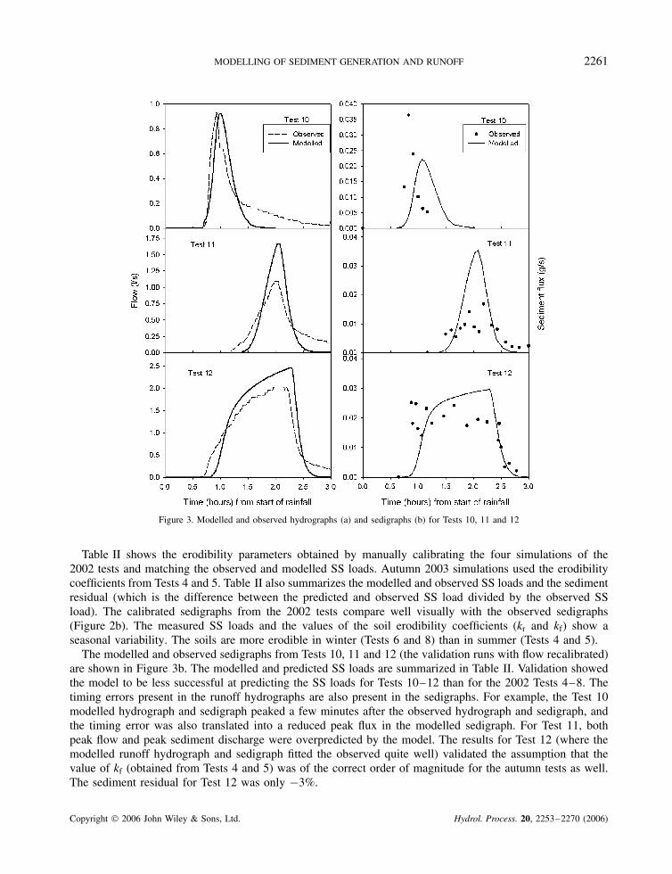
Figure 3. Modelled and observed hydrographs (a) and sedigraphs (b) for Tests 10, 11 and 12

Table II shows the erodibility parameters obtained by manually calibrating the four simulations of the2002 tests and matching the observed and modelled SS loads. Autumn 2003 simulations used the erodibilitycoefficients from Tests 4 and 5. Table II also summarizes the modelled and observed SS loads and the sedimentresidual (which is the difference between the predicted and observed SS load divided by the observed SSload). The calibrated sedigraphs from the 2002 tests compare well visually with the observed sedigraphs(Figure 2b). The measured SS loads and the values of the soil erodibility coefficients (kr and kf) show aseasonal variability. The soils are more erodible in winter (Tests 6 and 8) than in summer (Tests 4 and 5).

The modelled and observed sedigraphs from Tests 10, 11 and 12 (the validation runs with flow recalibrated)are shown in Figure 3b. The modelled and predicted SS loads are summarized in Table II. Validation showedthe model to be less successful at predicting the SS loads for Tests 10–12 than for the 2002 Tests 4–8. Thetiming errors present in the runoff hydrographs are also present in the sedigraphs. For example, the Test 10modelled hydrograph and sedigraph peaked a few minutes after the observed hydrograph and sedigraph, andthe timing error was also translated into a reduced peak flux in the modelled sedigraph. For Test 11, bothpeak flow and peak sediment discharge were overpredicted by the model. The results for Test 12 (where themodelled runoff hydrograph and sedigraph fitted the observed quite well) validated the assumption that thevalue of kf (obtained from Tests 4 and 5) was of the correct order of magnitude for the autumn tests as well.The sediment residual for Test 12 was only �3%.



Figure 4. Modelled and observed sedigraphs for Test 5 (concentrations)

The results from the model simulations of the autumn 2003 tests show that it is very important to fit theflow hydrograph first in order to fit the sedigraphs as well. Almost all the erosion was generated by overlandflow according to the model results, mainly because there was only 0Ð2% bare ground measured in the plot.Therefore, it was not possible to validate the calibrated summer value of kr properly. Moreover, this resultalso made the sediment results sensitive to the flow parameters, which is discussed below.

The modelled and observed concentrations are shown for Test 5 (Figure 4). During Test 5 the modelpredicted that the erosion was mostly due to raindrop detachment and that erosion occurred at a fairly constantrate controlled by the rainfall rate (Equation (1)). Therefore, the supply of sediment remained constant as therunoff increased during the rising limb, resulting in a gradual reduction in the SS concentrations. During thefalling limb the runoff decreased, but after the rain ceased so did the supply of eroded sediment, so the SSconcentrations continued to fall until runoff ceased.

Spatial erosion patterns

Figure 5a and b shows grid plots of the predicted rate of ground surface erosion for Tests 6 and 8respectively, when the surface runoff was near maximum (66 min after the start of the rainfall).

In the pre-grazing Test 6 (Figure 5a), the greatest erosion took place in central areas of the plot where therunoff from the outer regions of the plot converged to flow downhill to the outlet. This is consistent with theerosion being predominantly caused by overland flow when there is very high ground cover. Outer areas nearthe edge of the plot were subject to very low erosion rates, predominantly due to raindrop detachment (lessthan 0Ð005 mm day�1). In the microchannels, erosion rates were locally much higher (up to 0Ð3 mm day�1).The mean erosion rate across the entire plot was 0Ð012 mm day�1.

In the post-grazing Test 8 (Figure 5b), where there was less ground cover, large areas of the plotwere predicted to experience an erosion rate due to raindrop detachment of approximately 0Ð22 mm day�1.However, in the microchannels, where surface runoff was concentrated along narrow valleys in the centre ofthe plot, the erosion rates were lower on average (less than 0Ð1 mm day�1) due to the presence of surface watershielding these areas from raindrop detachment. The mean erosion rate was 0Ð2 mm day�1. The distributionof areas with high and low erosion rates was, therefore, almost the reverse of the distribution predicted duringTest 6.



Figure 5. Predicted rate of ground surface erosion (66 min after rain started): (a) Test 6; (b) Test 8

Figure 6. Rate of ground surface erosion time series plot: Test 8

Figure 6 shows time-series plots of the predicted rate of ground surface erosion at three selected gridelements during Test 8 (location shown in Figure 5a). The explanation for the differences between the erosionrates at the three locations is similar to the explanation of the spatial variation in erosion rate. At the edge ofthe plot (elements 2580 and 3250) the erosion was mainly due to raindrop detachment and predicted to take



place at an almost constant rate. At these outer elements the erosion rate decreased sharply as the rainfallstopped. In the centre of the plot (element 356, which is located in one of the microchannels) the rate wassimilar to the rate predicted at elements 2580 and 3250. Once runoff increased, surface water accumulatedon the grid square and reduced significantly the rate of erosion by raindrop detachment. The process ofoverland flow erosion generated less sediment in the microchannel than generated by raindrop detachment atthe outer grid squares. Some overland flow erosion was predicted to continue after the rain stopped as therunoff decreased, until finally ceasing around 1Ð8 h after the rain started.

The sediment transport predicted by the model was predominantly supply limited. According to the model,loose material eroded by raindrop detachment at the start of the simulation was transported down the plot bythe runoff once the runoff rate increased sufficiently for the transport capacity to rise (after around 20 min).Figure 4 showed that both the modelled and observed SS concentrations decreased during Test 5 as the flowincreased during the rising limb of the hydrograph and that the SS concentrations continued to fall duringthe falling limb as the amount of eroded material being transported reduced over time. The results indicatedthat transport capacity did not reach the maximum for the sizes of sediment particles used in the model, sincealmost all the eroded material was transported to the flume. The model predicted that no loose material wasdeposited on the grid elements until the end of the simulation when the runoff ceased.

Sensitivity analysis

The sensitivity of the predicted SS load to the erodibility coefficients and the percentage of bare groundwere assessed for Test 6 (winter pre-grazing) and Test 8 (winter post-grazing). Simulations of Tests 4 and 6,where raindrop detachment was the main erosion process, were insensitive to changes in the flow parameters.In fact, changes to the values of Kv, kstr and So have no effect on the rate of erosion by raindrop detachmentunless the amount of surface water on the ground surface can be drastically increased to shield the groundfrom raindrop detachment. Sensitivity (or elasticity of response, using terminology associated with economics)εij (dimensionless) of a model output j to a parameter i can be calculated by

εij D[

Oij/Oij

pi/pi

]�6�

where Oij is the change in model output j produced by a change (pi) in the value of parameter i, pi isthe arithmetic mean of the parameter values, and Oij is the arithmetic mean of the corresponding values ofthe output variable Oij.

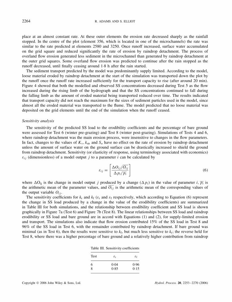
The sensitivity coefficients for kr and kf (εr and εf respectively, which according to Equation (6) representthe change in SS load produced by a change in the value of the erodibility coefficients) are summarizedin Table III for both simulations, and the relationship between erodibility coefficient and SS load is showngraphically in Figure 7a (Test 6) and Figure 7b (Test 8). The linear relationships between SS load and raindroperodibility or SS load and bare ground are in accord with Equations (1) and (2), for supply-limited erosionand transport. The simulations also indicate that flow erosion contributed 15% of the SS load in Test 8 and96% of the SS load in Test 6, with the remainder contributed by raindrop detachment. If bare ground wasminimal (as in Test 6), then the results were sensitive to kf, but much less sensitive to kr; the reverse held forTest 8, where there was a higher percentage of bare ground and a relatively higher contribution from raindrop

Table III. Sensitivity coefficients

Test εr εf

6 0Ð04 0Ð968 0Ð85 0Ð15



Figure 7. Sensitivity plots for (a) Test 6, (b) Test 8

detachment. As all the SS load was generated by the model using a combination of raindrop detachment andflow erosion, and the erosion was supply limited, the sum of εr and εf was 1Ð0 for both tests.

The effect of varying the flow parameters (Kv, kstr and So) on the SS load was investigated for Test 10(Figure 8). This test was selected since this simulation required recalibration of these parameters. The originalvalues obtained by calibration were 0Ð5 m1/3 s�1 for kstr, 4Ð8 mm h�1 for Kv and 1Ð2 m for So. Since thesediment residual for Test 10 was C33Ð2%, a reduction of the SS load by this percentage was required. Thechange in the flow parameters to achieve this change in SS load can be estimated graphically (Figure 8), andthe revised values were 5Ð1 mm h�1 for Kv, and 1Ð26 m for So, so the adjustments were relatively small.However, running a simulation using these parameter values would underpredict the runoff volume and peakrunoff (therefore reducing the quality of the flow simulation that had previously successfully predicted thepeak runoff).

The predicted SS load was most sensitive to the value of So and slightly less sensitive to Kv. It waspossible to increase either of these parameters by between 30 and 60% to generate zero runoff at the outletand, therefore, zero sediment load (i.e. change in sediment load of �100%).



Figure 8. Sensitivity analysis of sediment results to flow parameters for Tests 4 and 10 (10 unless stated otherwise)

The Strickler coefficient had a complicated and non-linear effect on the total SS load from Test 10. Therate of erosion was affected through changes in the shear stress and flow depth, both of which are affectedby this coefficient. It also affected the timing of the start of runoff and sediment discharge. A reduction ofkstr below 0Ð5 m1/3 s�1 generated less erosion, as the runoff was also reduced considerably despite the factthat the reduced value made the ground surface rougher and increased the surface water depth. Values ofkstr between 0Ð5 and 4Ð5 increased the overland flow erosion (but not by a large amount), since the runoffvolume increased. A value of kstr greater than 4Ð5 m1/3 s�1 reduced the overland flow resistance sufficiently toincrease the velocity and reduce the surface water depth, therefore generating less overland flow erosion. Anoptimum value of kstr (for a zero SS load residual) would be approximately 0Ð375 m1/3 s�1. The relationshipbetween the Strickler coefficient and SS load is also plotted for Test 4, where the runoff volume was anorder of magnitude higher than in Test 10. In this simulation, reducing the value of kstr increased the SS load,because making the ground surface rougher increased the surface water depth and shear stress. Conversely,increasing kstr decreased the surface water depth and likewise the SS load. The effect of changing kstr on therunoff volume (in percentage terms) was minimal in Test 4 compared with Test 10, and the effect of kstr onboth the runoff and SS load was as expected from the physical equations used in the model.

DISCUSSION

Both erosion processes (raindrop detachment and overland flow erosion) appeared to take place on the rainfallsimulator plot. The dominant erosion process depended on the amount of bare ground in the simulator plot.A sensitivity analysis showed that the predicted SS load was sensitive to either erodibility coefficient, butnot both, depending on the area of bare ground. The model simulations predicted that the overland flowerosion process (i.e. shear entrainment) was the dominant process at times when there had been no grazingin the rainfall simulator plot and the pasture cover was good. Raindrop erosion was the dominant generatorof sediment during the post-grazing rainfall simulator tests, when the amount of bare ground was significant.These post-grazing tests generated up to 30 times more SS than the corresponding pre-grazing tests, so itis important to model the process with a correct raindrop erodibility coefficient kr and a measurement orassessment of the ground cover. The physical basis for the seasonal variations in the values of the erodibilitycoefficients can be explained by changes in the soil cohesive strength. In summer and autumn the surface



soils are hard and less erodible than in winter and spring, when they are softer and more erodible, partlydue to increased soil moisture. The seasonal variation in the values of both the erodibility coefficients wasconsistent with the results of the earlier small rainfall simulator experiments carried out locally.

The calibrated values of the overland flow erodibility kf are much lower than those obtained from fieldstudies in the Iowa State University (ISU) catchments reported in Wicks and Bathurst (1996), which rangedfrom 0Ð14 to 0Ð41 mg m�2 s�1 compared with 4Ð5 ð 10�4 to 1Ð9 ð 10�3 mg m�2 s�1 from our study. Fromthe ISU catchments, kr varied from 28 to 82 J�1, compared with 2Ð3 to 12 J�1 in our study. From simulationsof rainfall simulator plots in Reynolds Creek, Idaho, Wicks et al. (1992) obtained, by calibration, values of1Ð3 J�1 for kr on grazed and ungrazed plots; this value of kr was closer to those obtained from our study.The calibrated value of kf from the same plots was 0Ð65 mg m�2 s�1, which again was several orders ofmagnitude greater than the values obtained from our study. Therefore, the soil in our rainfall simulator plotwould appear to be less erodible than the soils in both the US experimental catchments on the basis ofthe calibrated erodibility coefficients. The sediment yields from the ISU catchments ranged from 196 to3255 kg ha�1 for three modelled events (Wicks and Bathurst, 1996). The yields from our experiments (loaddivided by simulator area) were much lower, ranging from 0Ð4 kg ha�1 from Test 10 to 120 kg ha�1 fromTest 8).

Another explanation for the differences between the overland flow erodibility values obtained from theseearlier studies and this study is that this parameter might be scale dependent. The calibrated values obtainedby simulations described by Wicks and Bathurst (1996) used 25 m ð 25 m grid squares to model the ISUcatchments (which were of the order of 1 ha in size). The simulations described by Wicks et al. (1992) useda predecessor of SHETRAN and a single grid square to model a 32Ð54 m2 runoff plot. Using such a largegrid square would have removed any small-scale topographic features (e.g. microchannels) from the model.These features could have generated locally much higher rates of overland flow and erosion than average.Therefore, with a finer grid it may be possible to generate the same SS load at the plot outlet as the singlegrid square, but with a lower value of kf than the value obtained by the earlier study.

The measured surface runoff from the autumn 2003 tests was much lower than from the 2002 tests, probablydue to a larger initial soil moisture deficit (despite pre-wetting the plot) and also to vertical cracks in theclayey topsoil, which could have generated macropore flow and increased Kv. The measured SS loads fromthe autumn 2003 tests were also lower as a result of the lower runoff in conjunction with lower erodibility.The validation results from the model simulations of Tests 10–12 indicated that the value of the overlandflow erodibility in autumn was very similar to that in summer. This result was achieved by showing that theresidual error in the SS load from one of the Tests (12) was very small.

Measured SS loads from the rainfall simulator plot, generated by the artificial rainfall, were low apart fromTest 8 (winter post-grazing).) Yields were also low compared with an estimated average yield at Mangaotama(a larger 2Ð6 km2 catchment adjacent to the paddock containing the simulator plot) of 2100 kg ha�1 year�1

(Quinn and Stroud, 2002). Elliott and Carlson (2004) estimated that the average yield from the larger 3 haPukemanga catchment (which contains the rainfall simulator plot) was only 20 kg ha�1 year�1. It is probablethat other erosion processes (bank erosion, small landslides, sediment washed from unsealed roads, etc.) aretaking place in the larger Mangaotama catchment (Quinn and Stroud, 2002).

CONCLUSIONS

The values for the two erodibility coefficients used by SHETRAN varied seasonally, and this variation wasconsistent with the results of the previous small rainfall simulator experiments carried out in different seasonsin the vicinity of our large rainfall simulator. The erodibility coefficients were lower than those obtained fromthe ISU runoff plot studies in the USA. The raindrop erodibility kr values were still of the same order ofmagnitude, but the overland flow erodibility kf values were several orders of magnitude smaller. The results



(both observed sediment yields and erodibility coefficient values) indicate that the soil in the rainfall simulatorplot is less erodible than the silt loam soils in the ISU catchment.

It is important to fit the runoff hydrograph successfully, since the sediment results are sensitive to theparameters that control the flow results, especially if overland flow erosion is the dominant erosion mechanismin the simulator plot (when the area of bare ground is small).

Rill initiation was not observed in the plot after any of the experiments. Therefore, the surface soil underthe rainfall simulator does not appear to be very susceptible to overland flow erosion by either interrill orrill processes. Therefore, the important conclusion for land management is that ensuring good pasture coveris important to restrict the amount of sediment generated by large rainfall events on hillslopes with similarslopes and soils to Pukemanga, particularly in winter.

The SHETRAN model is a useful tool for predicting spatial patterns of erosion under the rainfall simulator(Figure 6). Validation of these patterns against field measurements was not possible. More research effort isrequired to identify values for the erodibility coefficients a priori when running sediment transport simulationsto avoid having to calibrate these coefficients for each new application, or alternatively upper and lower boundsto the parameter values could be used based on previous applications.

Scale effects in the parameters that describe the overland flow erosion process may be important andrequire further investigation, especially if the model is to be applied to different size catchments with largergrid elements, in the vicinity of the current field site at Whatawhata.

ACKNOWLEDGEMENTS

We would like to thank the following: the members of the ‘Pukemanga Working Group’, from AgResearchLtd, Landcare Research Ltd and Lincoln Environmental Ltd, who contributed to the study; Professor EndaO’Connell, Dr Geoff Parkin, Dr James Bathurst and Dr Steve Birkinshaw at the School of Civil Engineeringand Geosciences, University of Newcastle Upon Tyne (UK), for their assistance with the SHETRAN software;Todd Williston (NIWA) for his assistance with the fieldwork; the AgResearch farm staff at Whatawhata; DrKit Rutherford and Graham McBride (the internal reviewers) for their constructive comments.

APPENDIX A: NOTATION

c Sediment concentration (m3 m�3)CC Proportion of ground covered by a canopyCG Proportion of ground covered by ground vegetationDF Rate of detachment of soil per unit area by overland flow (kg m�2 s�1)DR Rate of soil detachment by a combination of leaf drip and raindrop impact (kg m�2 s�1)D50 Representative median diameter of soil particle (mm)εij Sensitivity of output j to variable iεr Sensitivity of SS load to raindrop erodibility coefficientεf Sensitivity of SS load to overland flow erodibility coefficientFW Correction factor for shielding ground surface from raindrop impactgx Sediment transport rate (m3 s�1 m�1) in the x directiongy Sediment transport rate (m3 s�1 m�1) in the y directionh Depth of water (m)Kv Vertical hydraulic conductivity (mm h�1)kr Raindrop soil erodibility coefficient (J�1)kf Overland flow soil erodibility coefficient (kg m�2 s�1)kstr Strickler coefficient (m1/3 s�1)� Soil surface porosity



MD Momentum-squared for leaf drip �kg2 m�3�MR Momentum-squared for rain �kg2 m�3�O Output (used in sensitivity analysis)p Parameter value (used in sensitivity analysis)� Density of water (kg m�3)Sf Friction slopeSo Initial phreatic surface depth (m)t Time (s)� Actual shear stress (N m�2)�c Critical shear stress (N m�2)u Velocity (m s�1)z Depth of loose soil (m)

REFERENCES

Abbott MB, Bathurst JC, Cunge JA, O’Connell PE, Rasmussen J. 1986. An introduction to the European Hydrological System–the SystemeHydrologique Europeen. Journal of Hydrology 87(1–2): 45–59.

Adams R, Parkin G, Rutherford JC, Ibbitt RP, Elliott AH. 2005. Using a rainfall simulator and a physically based hydrological model toinvestigate runoff processes in a hillslope. Hydrological Processes 19: 2209–2223. DOI: 10.1002/hyp.5670.

APHA. 1995. Standard Methods for the Examination of Water and Wastewater , 19th edn. American Public Health Research Association:Washington, DC.

Bathurst JC, Wicks JM, O’Connell PE. 1995. The SHE/SHESED basin scale water flow and sediment transport modelling system. InComputer Models of Watershed Hydrology , Singh VP (ed.). Water Resources Publications LLC: Highlands Ranch, CO; 563–594.

Bowyer-Bower TAS, Burt TP. 1989. Rainfall simulators for investigating soil response to rainfall. Soil Technology 2: 1–16.Campbell DA. 1945. Soil-conservation studies applied to farming in Hawke’s Bay. New Zealand Journal of Science and Technology, Section

A: Agricultural Research Section 26: 301–332.Christiansen JE. 1942. Irrigation by sprinkling . University of California Agricultural Experiment Station Bulletin 670.Elliott AH, Carlson WT. 2004. Effects of sheep grazing episodes on sediment and nutrient loss in overland flow. Australian Journal of Soil

Research 42: 213–220. DOI: 10.1071/SR02111.Elliott AH, Tian YQ, Rutherford JC, Carlson WT. 2002. Effect of cattle treading on interrill erosion from hill pasture: modelling concepts

and analysis of rainfall simulator data. Australian Journal of Soil Research 40(6): 963–976. DOI: 10.1071/SR01057.Ewen J, Parkin G, O’Connell PE. 2000. SHETRAN: distributed river basin flow and transport modeling system. Journal of Hydrologic

Engineering 5: 250–258.Ewen J, Bathurst JC, Parkin G, O’Connell PE, Birkinshaw SJ, Adams R, Hiley R, Kilsby CG, Burton A. 2002. SHETRAN: physically-

based distributed river basin modelling system. In Mathematical Models of Small Watershed Hydrology and Applications , Singh VP,Frevert DK (eds). Water Resources Publications LLC: Highlands Ranch, CO; 43–68.

Harrod TR, Theurer FD. 2003. Sediment. In Agriculture, Hydrology and Water Quality: Section 1. Agriculture: Potential Sources of WaterPollution, Haygarth PM, Jarvis SC (eds). CABI Publishing: Wallingford; 155–170.

Lambert MG, DeVantier BP, Nes P, Penney PE. 1985. Losses of nitrogen, phosphorus and sediment in runoff from hill country underdifferent fertiliser and grazing management regimes. New Zealand Journal of Agricultural Research 28: 371–379.

Lane PNJ, Croke JC, Dignan P. 2004. Runoff generation from logged and burnt out hillslopes: rainfall simulation and modelling.Hydrological Processes 18: 879–892. DOI: 10.1002/hyp.1316.

Mantz PA. 1977. Incipient transport of fine grains and flakes by fluids—extended Shields diagram. Journal of the Hydraulics Division,ASCE 103(6): 601–615.

McColl RHS, Gibson AR. 1979. Downslope movement of nutrients in hill pasture, Taita, New Zealand. II. Effects of season, sheep grazingand fertiliser. New Zealand Journal of Agricultural Research 22: 151–161.

Muller K, Adams R, Stenger R. 2004. Soils in the Pukemanga catchment with emphasis on hydraulic properties . AgResearch Client Reportfor Pukemanga Working Group, March.

Nash JE, Sutcliffe JV. 1970. River flow forecasting through conceptual models: 1, a discussion of principles. Journal of Hydrology 10:282–290.

Nguyen ML, Sheath GW, Smith CM, Cooper AB. 1998. Impact of cattle treading on hill land 2. Soil physical properties and contaminantrunoff. New Zealand Journal of Agricultural Research 41: 279–290.

Quinn JM, Stroud MJ. 2002. Water quality and sediment and nutrient export from New Zealand hill-land catchments of contrasting landuse. New Zealand Journal of Marine and Freshwater Research 36: 409–429.

Seelhorst B, Wickop E. 1994. Erodibility of soils in relation to different landuse in the Kiripaka catchment (Hakarimata ranges), WhatawhataResearch Farm, North Island, New Zealand . Georg August University of Goettingen Report.

Selby MJ. 1972. The relationships between landuse and erosion in the central North Island, New Zealand. Journal of Hydrology (NewZealand) 11: 73–87.



Wicks JM, Bathurst JC. 1996. SHESED: a physically based, distributed erosion and sediment yield component for the SHE hydrologicalmodelling system. Journal of Hydrology 175: 213–238.

Wicks JM, Bathurst JC, Johnson CW. 1992. Calibrating SHE soil-erosion model for different land covers. Journal of Irrigation and DrainageEngineering, ASCE 118(5): 708–723.

Wischmeier WH, Smith DD. 1978. Predicting Rainfall Erosion Losses , USDA Agricultural Handbook No. 537. Agricultural Research Service:Washington, DC.

Yalin MS. 1963. An expression for bed-load transportation. Journal of the Hydraulics Division, ASCE 89: 221–250.


Physically based modelling of sediment generation and transport under a large rainfall simulator

Documents

Transcript of Physically based modelling of sediment generation and transport under a large rainfall simulator