Physically Based Evaporative Demand as a Drought Metric ... · Physically Based Evaporative Demand...

University of Nevada, Reno

Physically Based Evaporative Demand as a Drought Metric: Historical Analysis and

Seasonal Prediction

A dissertation submitted in partial fulfillment of the requirements for the degree of

Doctor of Philosophy in Atmospheric Science

by

Daniel J. McEvoy

Dr. John Mejia/Dissertation Advisor

August, 2015

We recommend that the dissertation

prepared under our supervision by

DANIEL J. MCEVOY

Entitled

Physically Based Evaporative Demand As A Drought Metric: Historical Analysis

And Seasonal Prediction

be accepted in partial fulfillment of the

requirements for the degree of

DOCTOR OF PHILOSOPHY

Dr. John Mejia, Advisor

Dr. Timothy Brown, Committee Member

Dr. Eric Wilcox, Committee Member

Dr. Mike Hobbins, Committee Member

Dr. Justin Huntington, Graduate School Representative

David W. Zeh, Ph. D., Dean, Graduate School

August, 2015

THE GRADUATE SCHOOL

i

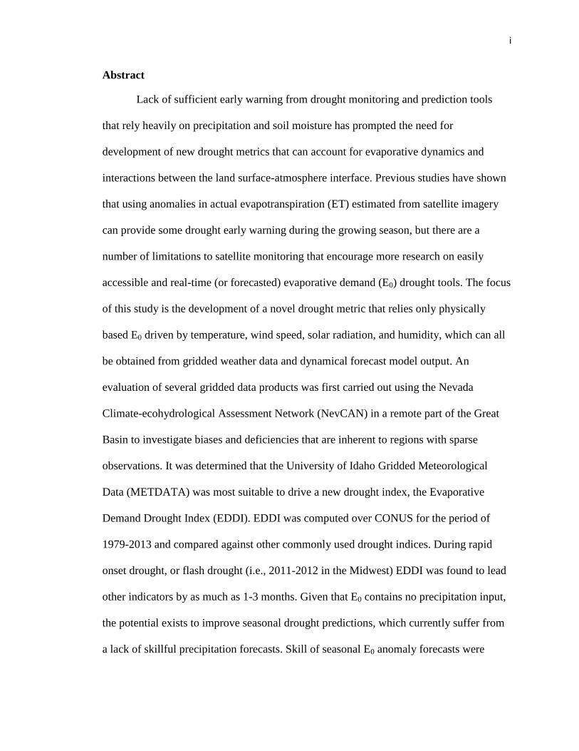
Abstract

Lack of sufficient early warning from drought monitoring and prediction tools

that rely heavily on precipitation and soil moisture has prompted the need for

development of new drought metrics that can account for evaporative dynamics and

interactions between the land surface-atmosphere interface. Previous studies have shown

that using anomalies in actual evapotranspiration (ET) estimated from satellite imagery

can provide some drought early warning during the growing season, but there are a

number of limitations to satellite monitoring that encourage more research on easily

accessible and real-time (or forecasted) evaporative demand (E0) drought tools. The focus

of this study is the development of a novel drought metric that relies only physically

based E0 driven by temperature, wind speed, solar radiation, and humidity, which can all

be obtained from gridded weather data and dynamical forecast model output. An

evaluation of several gridded data products was first carried out using the Nevada

Climate-ecohydrological Assessment Network (NevCAN) in a remote part of the Great

Basin to investigate biases and deficiencies that are inherent to regions with sparse

observations. It was determined that the University of Idaho Gridded Meteorological

Data (METDATA) was most suitable to drive a new drought index, the Evaporative

Demand Drought Index (EDDI). EDDI was computed over CONUS for the period of

1979-2013 and compared against other commonly used drought indices. During rapid

onset drought, or flash drought (i.e., 2011-2012 in the Midwest) EDDI was found to lead

other indicators by as much as 1-3 months. Given that E0 contains no precipitation input,

the potential exists to improve seasonal drought predictions, which currently suffer from

a lack of skillful precipitation forecasts. Skill of seasonal E0 anomaly forecasts were

ii

assessed over CONUS using the Climate Forecast Version 2 (CFSv2) hindcasts for 1982-

2009 and METDATA was used as baseline observations. E0 forecast skill during drought

events was consistently greater than precipitation, with much improved skill over parts of

the central and northeast U.S. during the growing season. Results from this study suggest

that continued efforts should be put towards incorporating physically based E0 in

operational drought monitoring and prediction frameworks.

iii

Acknowledgements

I would like to thank my family for continued support throughout this long

journey, especially my mother, Ilene McEvoy, and my wife, Heather McEvoy. Many

thanks to my committee members; I could not have made it this far without their expert

knowledge and guidance. I would especially like to thank Dr. John Mejia and Dr. Justin

Huntington for having confidence in me to largely choose my own path and take charge

of my dissertation topics. There is a long list of DRI graduate students who I would like

to thank for help and support along the way, particularly with the steep learning curve

associated with scientific programming. I’m extremely thankful that I got the opportunity

to experience this challenging task, and the experience will stick with me for the rest of

my life. I would like to dedicate this work to my two year daughter, Sierra McEvoy, and

my two week old son, Sage McEvoy.

iv

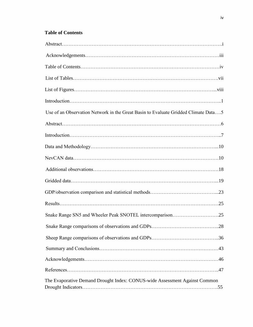
Table of Contents

Abstract…………………………………………………………………………………….i

Acknowledgements………………………………………………………………………iii

Table of Contents…………………………………………………………………………iv

List of Tables…………………………………………………………………………….vii

List of Figures…………………………………………………………………………...viii

Introduction………………………………………………………………………………..1

Use of an Observation Network in the Great Basin to Evaluate Gridded Climate Data….5

Abstract……………………………………………………………………………………6

Introduction………………………………………………………………………………..7

Data and Methodology…………………………………………………………………...10

NevCAN data…………………………………………………………………………….10

Additional observations………………………………………………………………….18

Gridded data……………………………………………………………………………...19

GDP/observation comparison and statistical methods…………………………………...23

Results……………………………………………………………………………………25

Snake Range SN5 and Wheeler Peak SNOTEL intercomparison……………………….25

Snake Range comparisons of observations and GDPs…………………………………..28

Sheep Range comparisons of observations and GDPs…………………………………..36

Summary and Conclusions………………………………………………………………43

Acknowledgements………………………………………………………………………46

References………………………………………………………………………………..47

The Evaporative Demand Drought Index: CONUS-wide Assessment Against Common

Drought Indicators……………………………………………………………………….55

v

Abstract…………………………………………………………………………………..56

Introduction………………………………………………………………………………57

Data and methods………………………………………………………………………...60

Evaporative demand……………………………………………………………………...60

Evaporative Demand Drought Index…………………………………………………….61

NLDAS-based drought metrics…………………………………………………………..62

Evaporative Stress Index…………………………………………………………………63

United States Drought Monitor…………………………………………………………..64

Results and Discussion…………………………………………………………………..65

NLDAS-2 drought index correlations with EDDI……………………………………….65

ESI correlations with EDDI……………………………………………………………...72

Flash drought over the central US……………………………………………………….74

Extended drought in arid to semi-arid regions…………………………………………...80

Summary and Conclusions………………………………………………………………84

Acknowledgements………………………………………………………………………87

References………………………………………………………………………………..87

Exploring the use of Physically Based Evaporative Demand Anomalies to Improve

Seasonal Drought Forecasts……………………………………………………………...96

Abstract…………………………………………………………………………………..97

Introduction………………………………………………………………………………98

Data and methodology………………………………………………………………….101

Results…………………………………………………………………………………105

Deterministic skill………………………………………………………………………105

Categorical skill of probability forecasts in drought events……………………………115

vi

ENSO as a source of predictability……………………………………………………..118

Discussion and conclusions…………………………………………………………….119

Acknowledgements……………………………………………………………………..123

References………………………………………………………………………………123

Summary and Conclusions……………………………………………………………..127

vii

List of Tables

Use of an Observation Network in the Great Basin to Evaluate Gridded Climate Data

Table 1. Summary of station locations, elevations, measured variables (where T indicates

temperature), measurement frequency, and precipitation gauge information (where TB

indicates tipping bucket)………………………………………………………………….12

Table 2. Geonor rain gauge and tipping bucket rain gauge comparison

statistics…………………………………………………………………………………..16


Drought Indicators

Table1. Drought classes for comparing USDM to SPI, SSI, ESI, and EDDI……………64

Exploring the Use of Physically Based Evaporative Demand Anomalies to Improve

Seasonal Drought Forecasts

Table 1. CFSv2 monthly ensembles are listed and each initial day consists of four

members initialized at 00Z, 06Z, 12Z, and 18Z………………………………………102

viii

List of Figures

Use of an Observation Network in the Great Basin to Evaluate Gridded Climate Data

Figure 1. (A) Study area with insets indicating locations of the Snake and Sheep Ranges.

Close-up of the (B) Snake Range and (C) Sheep Range with red dots indicating station

locations. Zoomed-in frame (B) highlights the close proximity of Wheeler Peak SNOTEL

(WPS) to NevCAN. Station summaries can be found in Table 1………………………..13

Figure 2. Time series of Geonor rain gauge (black line) and tipping bucket rain gauge

(green line) precipitation at SN2 during the (a) cold season and (b) warm season.

Abscissa tick marks indicate date (MM/DD)…………………………………………….17

Figure 3. Water year 2012 total precipitation [mm] at the Snake Range for (a) PRISM 4-

km, (b) PRISM 800-m, (c) JA 4-km, and (d) Daymet 1-km…………………………….22

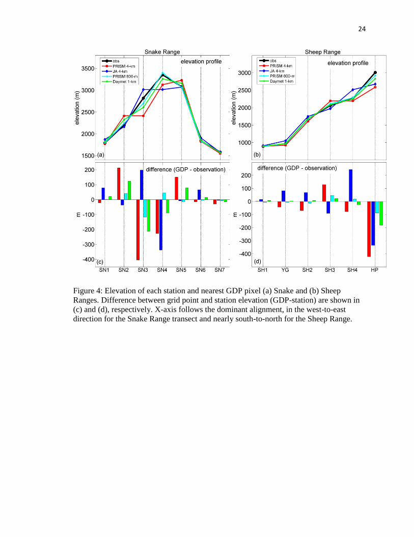
Figure 4. Elevation of each station and nearest GDP pixel (a) Snake and (b) Sheep

Ranges. Difference between grid point and station elevation (GDP-station) are shown in

(c) and (d), respectively. X-axis follows the dominant alignment, in the west-to-east

direction for the Snake Range transect and nearly south-to-north for the Sheep Range...24

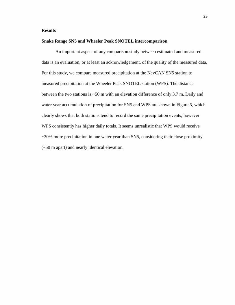
Figure 5. NevCAN SN5 (black) and WPS (magenta) daily precipitation totals (a) and

accumulated precipitation (b) throughout the water year. Abscissa tick marks indicate

date (month-year)………………………………………………………………………...26

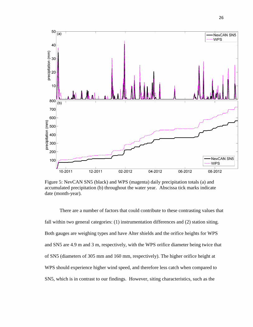
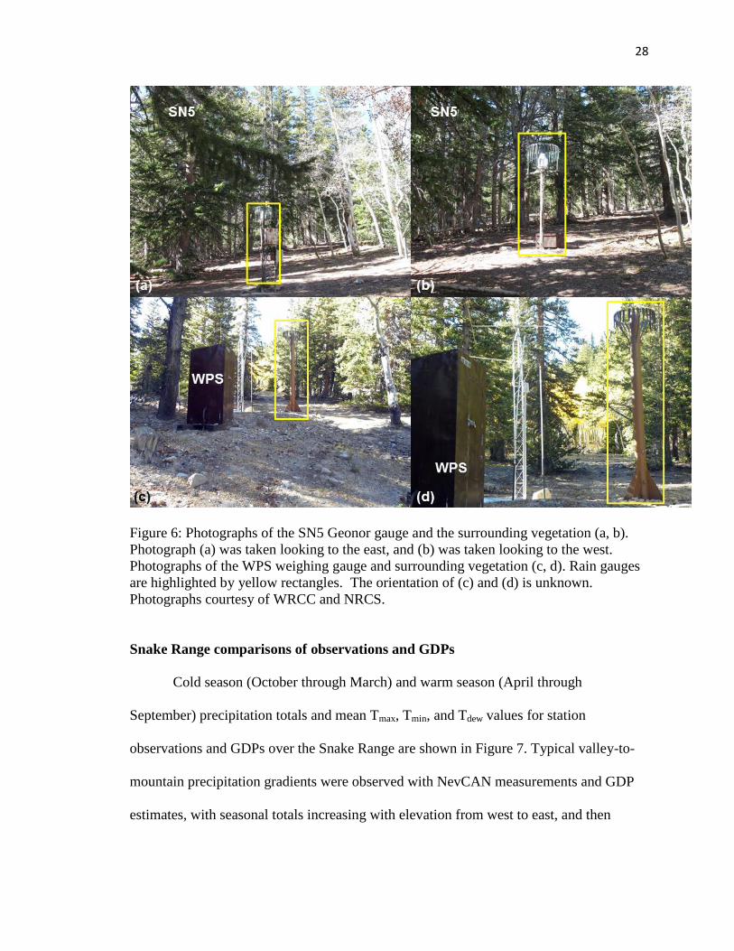
Figure 6. Photographs of the SN5 Geonor gauge and the surrounding vegetation (a, b).

Photograph (a) was taken looking to the east, and (b) was taken looking to the west.

Photographs of the WPS weighing gauge and surrounding vegetation (c, d). Rain gauges

are highlighted by yellow rectangles. The orientation of (c) and (d) is unknown.

Photographs courtesy of WRCC and NRCS……………………………………………..28

Figure 7. Snake Range seasonal precipitation totals (a, b) and seasonal mean Tmax (c, d),

Tmin (e, f), and Tdew (g, h). Cold season is shown on the left (a, c, e, g) and warm season

on the right (b, d, f, h). X-axis is aligned west to east (left to right)……………………..32

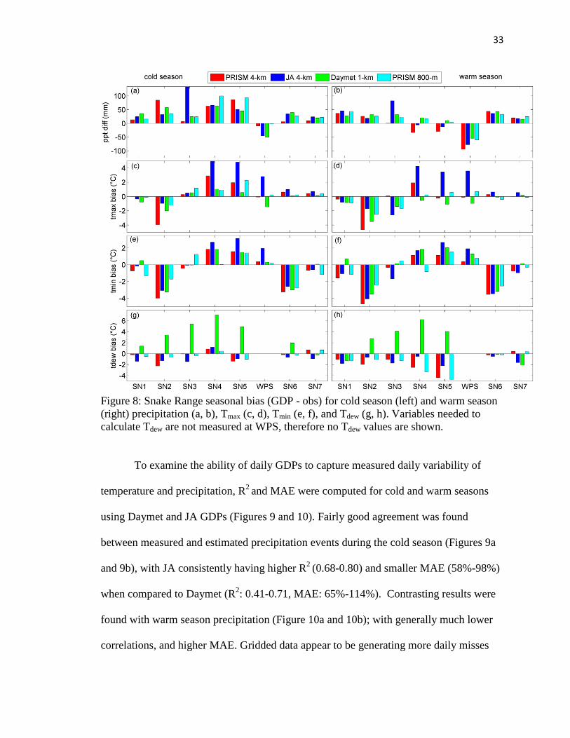
Figure 8. Snake Range seasonal bias (GDP - obs) for cold season (left) and warm season

(right) precipitation (a, b), Tmax (c, d), Tmin (e, f), and Tdew (g, h). Variables needed to

calculate Tdew are not measured at WPS, therefore no Tdew values are shown…………..33

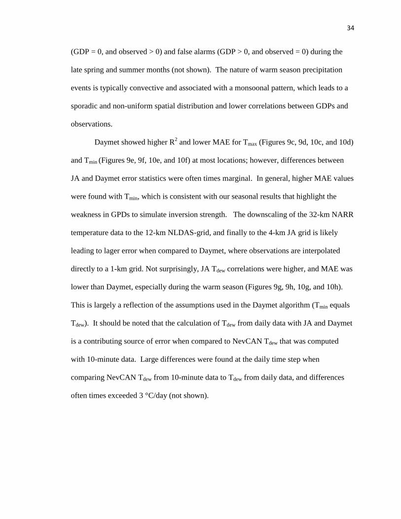
Figure 9. Snake Range cold season R2 (left) and MAE (right) computed at the daily time

step for precipitation (a, b), Tmax (c, d), Tmin (e, f), and Tdew (g, h) using Daymet and JA.

For precipitation, MAE is expressed as a percentage, while MAE for Tmax, Tmin, and Tdew

is expressed in °C………………………………………………………………………...35

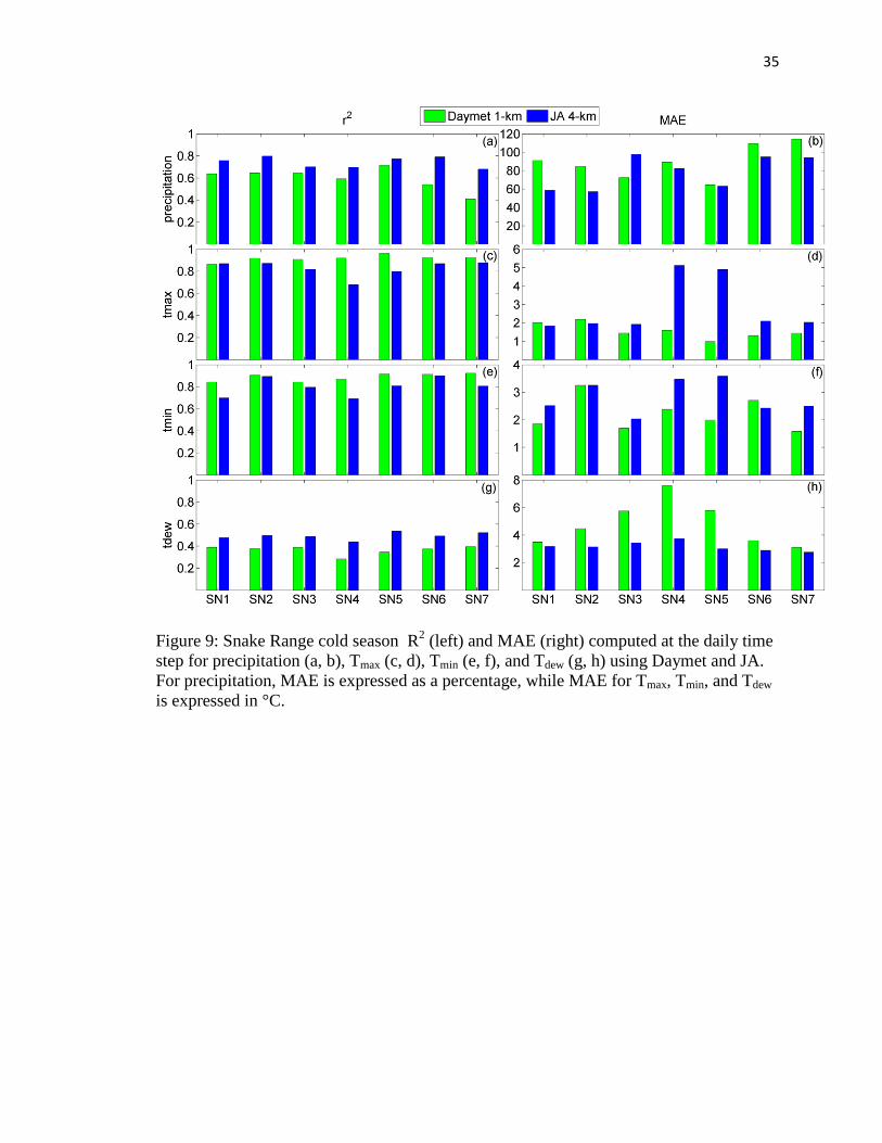
Figure 10. Snake Range warm season R2 (left) and MAE (right) computed at the daily

time step for precipitation (a, b), Tmax (c, d), Tmin (e, f), and Tdew (g, h) using Daymet and

JA. For precipitation, MAE is expressed as a percentage, while MAE for Tmax, Tmin, and

Tdew is expressed in °C…………………………………………………………………...36

Figure 11. Sheep Range seasonal precipitation totals (a, b) and seasonal mean Tmax (c, d),


on the right (b, d, f, h). X-axis is aligned west to east (left to right). For precipitation

observations, filled circles represent tipping bucket gauges, and filled upside down

triangles represent weighing gauges……………………………………………………..39

ix

Figure 12. Sheep Range seasonal bias (GDP - obs) for cold season (left) and warm season

(right) precipitation (a, b), Tmax (c, d), Tmin (e, f), and Tdew (g, h)……………………….40

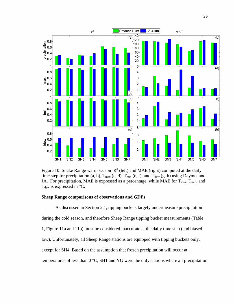
Figure 13. Sheep Range cold season R2 (left) and MAE (right) computed at the daily


JA. For precipitation, MAE is expressed as a percentage, while MAE for Tmax, Tmin,

and Tdew is expressed in °C……………………………………………………………..42

Figure 14. Sheep Range warm season R2 (left) and MAE (right) computed at the daily



Tdew is expressed in °C…………………………………………………………………...43


Drought Indicators

Figure 1. Correlation coefficient between EDDI and SPI at (a) 1-month, (c) 6-month, (e)

12-month, and SSI (b) 1-month, (d) 6-month, and (f) 12-month time scales……………66

Figure 2. Shading indicates METDATA terrain height (m) and red boxes indicate area-

averaging domains for Figures 3 and 4. IA, TX, and PA boxes are 50 x 100 4-km

METDATA pixels (200 km x 400 km), and CA box is 25 x 25 pixels (100 km x 100

km)……………………………………………………………………………………….67

Figure 3. Monthly correlations between EDDI and SPI (top row) and SSI (bottom row) at

all time scales for (a, e) TX, (b, f) CA, (c, g) IA, and (d, h) PA. Y-axis indicates ending

month of each time scale, and x-axis shows time scale (months). Shading indicates

correlation coefficients…………………………………………………………………...70

Figure 4. Lagged correlation between 3-month SSI ending in August and EDDI for (a)

CA, (b) TX, (c) IA, and (d) PA. Y-axis indicates EDDI ending months and x-axis

indicate EDDI time scale. Green dots are placed in the ending month containing the

strongest correlation for each time scale, and blue dots are used as a reference to show

SSI time scale and ending month………………………………………………………...72

Figure 5. Seasonal correlation coefficient (left column spring and right column summer)

between ESI and EDDI at (a, b) 4-week, (c, d) 8-week, and (e, f) 12-week time scales.

Areas shaded in white indicate an insufficient amount of ESI data……………………..74

Figure 6. EDDI under sustained and flash drought conditions. (a) Monthly time series of

1-month EDDI, SSI, and SPI area averaged over the IA domain. (b) Monthly time series

of 1-month EDDI and EDDI constrained by climatology Tair (EDDI-T), q (EDDI-q), Rd

(EDDI-Rd), and U2 (EDDI- U2). Black box highlights time period shown in (c). (c) Daily

time series of 1-month EDDI, EDDI-T, EDDI-q, EDDI-Rd and EDDI-U2 for May and

June 2011 shown to highlight details of flash drought initiation. Note that the vertical axis

of EDDI is reversed to clearly visualize drought onset and duration when compared to

SPI and SSI. Light green reference line indicates start of moderate drought classification

(-0.78)……………………….............................................................................................77

Figure 7. Evolution of the 1-month EDDI (top row), USDM (second row), 1-month ESI

(third row), 1-month SSI (fourth row), and 1-month SPI (fifth row) through spring and

summer of 2012. USDM data are from 1 May, 2012 (April column), 5 June, 2012 (May

x

column), 3 July, 2012 (June column), and 31 July, 2012 (July column). EDDI, ESI, SSI,

and SPI are at 1-month time scales at the end of each month: April, May, June, and July.

All drought metrics have been converted to USDM categories according to Table 1…..79

Figure 8. USDM from 02 October, 2007 (a) and 25 June, 2002 (b), 12-month (October-

September) EDDI (c), SSI (e), and SPI (g) ending September, 2007, and 6-month

(January-June) EDDI (d), SSI (f), and SPI (h) ending June, 2002………………………82

Figure 9. Area-averaged time series of EDDI over the northern Sierra Nevada from 1979

to 2013 aggregated at 2-week (a), 1-month (b), 3-month (c), 6-month (d), and 12-month

time scales………………………………………………………………………………..84



Figure 1. Accumulated E0 (a) and Prcp (b) anomaly percentiles from METDATA for

AMJ 2002. Note that upper E0 and lower Prcp percentiles indicate drought (brown

shading). NCDC climate regions (described in Section 2) used as area averaging domains

for Section 3 results are shown in the bottom panel (c). Regions are named as follows:

Northwest (NW), West (We), Southwest (SW), West North Central (WNC), South (So),

East North Central (ENC), Central (Ce), Southeast (SE), and Northeast (NE)………...100

Figure 2. CONUS average percent area in drought based on 3-month accumulated E0 (a)

and Prcp (b) percentiles………………………………………………………………...101

Figure 3. Comparison between 1982-2009 CONUS-average annual E0 from the

METDATA native grid of 4-km (x-axis) and the re-gridded 1° spatial resolution (y-

axis)……………………………………………………………………………………..103

Figure 4. Average ET0 anomaly correlation between METDATA and CFSRF over each

region (refer to Figure 1c for full region names and locations). Labels on the x-axis

indicate lead time (months) and labels on the y-axis indicate target month……………106

Figure 5: Average precipitation anomaly correlation between METDATA and CFSRF

over each region (refer to Figure 1c in main manuscript for full region names and

locations). Labels on the x-axis indicate lead time (months) and labels on the y-axis

indicate target month……………………………………………………………………107

Figure 6. As in Figure 4, but for maximum temperature……………………………….108

Figure 7. As in Figure 4, but for minimum temperature………………………………..109

Figure 8. As in Figure 4, but for specific humidity…………………………………….110

Figure 9. As in Figure 4, but for downwelling shortwave radiation at the surface…….111

Figure 10. As in Figure 4, but for wind speed………………………………………….113

Figure 11. Season-1 anomaly correlation area-averaged over CONUS and individual

climate regions. The black reference line is anomaly correlation of 0.3, which indicates

the start of moderate skill……………………………………………………………….115

Figure 12. The HSS for lead one-month, season-1 forecasts for cases when both E0 and

Prcp indicate drought (>80th

percentile for E0 and <20th

percentile for Prcp). Labels inside

of each panel indicate region and mean HSS. Red circles show notable drought events of

JFM, FMA, and MAM 1992 in the NW, JJA 1988 in the WNC, ENC, and Ce, JAS, ASO,

and SON 1999 in the Ce, and MJJ and JJA 1999 in the NE. These events are described in

further detail in the text…………………………………………………………………117

xi

Figure 13. The difference in AC (ENSO conditional forecasts – All forecasts) and

regionally averaged AC for E0 (a and c) and Prcp (b and d) forecasts…………………119

1

Introduction Drought is a costly and devastating type of natural disaster that leads to adverse

effects in many groups and sectors throughout the United States (US) including

agriculture, water resources, public health, outdoor recreation, and the national and global

economy. The 20th

century saw a number of severe droughts in the US, most notably the

Dust Bowl era of the 1930’s, but some of the most extreme events have occurred in the

first 15 years of the 21st century: 2000-2003 in the Southwest, 2011 in Texas, 2011-2012

in the Midwest, and 2012-present in California. Recent drought severity has been

exacerbated by high temperatures and increased evaporative demand (E0), and future

projections of a warming climate indicate that extreme drought events (like those of the

21st century) are likely to become more frequent and longer in duration. Improving

drought monitoring and prediction capabilities is therefore of utmost importance for the

US, and could reduce the damaging environmental and societal effects of drought by

providing much needed early warning. Improved early warning allows for reactive

emergency responses, implementation of actions within statewide and local drought

plans, and can provide essential information for decision support.

Precipitation, temperature, and soil moisture have been the most commonly used

variables in drought monitoring and prediction in the past. However, recent advances

have been made that primarily utilize the wealth of data provided by satellites and land

surface models (LSMs) to explore the utility of evapotranspiration (ET) and E0 as

drought indicators. Promising new research has shown that through interactions between

the land surface-atmosphere interface these variables (ET and E0) can often times provide

early warning over traditional drought metrics. Satellite data has been an invaluable

2

resource to geophysical scientists, but there a number of limitations to satellite

monitoring that encourage more research and development of easily accessible and real-

time (or forecasted) ET and E0 drought tools. Even with advanced satellites accurate

spatial estimates of ET continue to be a major challenge, making E0 estimates driven by

more commonly measured meteorological variables a more attractive option for drought

monitoring.

Over the past several decades a number of options have become available to

obtain data for estimation of physically based E0 (driven by temperature, humidity, wind

speed, and solar radiation) including LSMs, reanalysis of atmospheric models, and purely

statistical models where observations are spatially interpolated. A major challenge in

today’s data-rich world is determining which data source is best suited for a specific

application, such as E0 estimation, and unfortunately the consequences of these choices

are often overlooked.

The research in this dissertation is focused on improving drought monitoring and

predictions using physically based E0, and evaluating gridded climate data that may be

used for the application of estimating E0. The hypothesis and research questions for each

chapter are as follows:

1. It is hypothesized in Chapter 1 that in the complex terrain of the western US,

specifically the Great Basin, significant differences can be found in the variables

of precipitation, temperature, and humidity between several gridded data products

(GDPs) of varying spatial resolution, with higher resolution not always leading to

greater skill. Of particular interest are the impacts of low station density and

3

station siting on GDP precipitation estimates, and methodology and accuracy of

GDP humidity estimates, which are a critical component of physically based E0

estimates. In this research four GDPs are evaluated (ranging from 4-km to 800-m

spatial resolution) against a new observing network: the Nevada Climate-

ecohydrological Assessment Network (NevCAN).

2. Development and assessment of the first drought index based solely on physically

based E0, the Evaporative Demand Drought Index (EDDI), is presented in

Chapter 2. Based partially on several findings from Chapter 1, the 4-km

METDATA was chosen to calculate E0 using the physically based American

Society for Civil Engineers Standardized Reference ET (ET0) approach. A

calculation procedure for EDDI is presented, and EDDI is calculated over

CONUS for several aggregation time scales for the period of 1979-2013. EDDI is

then compared against several commonly used drought indices and the US

Drought Monitor. It is further hypothesized that EDDI can be a leading indicator

during rapid onset, or “flash” drought—conditions when ample moisture may still

be available at the surface (i.e., energy limited ET conditions) both due to both

advective and radiative meteorological forcings, ET and ET0 are driven in the

same direction, thus leading to a drought signal from EDDI and a wetting signal

from ET-based drought metrics. The hypothesis that EDDI can also serve as an

effective indicator of hydrologic drought in water-limited regions (based on the

classic complementary relationship between ET and ET0) using longer time scales

is also tested.

4

3. Seasonal drought prediction remains a challenge primarily due to poor skill in

long-term precipitation forecasts. Skill in seasonal temperature predictions is

significantly better than precipitation. However, temperature alone is not always

an accurate drought indicator. In Chapter 3, the hypothesis that predictions of

seasonal ET0 anomalies contain improved skill over precipitation anomaly

forecasts due largely to the sensitivity of ET0 to temperature is tested. Reforecast

data from the National Center for Environmental Prediction Climate Forecast

System Version 2 (CFSv2) is used to compute ET0 and evaluate both ensemble

(deterministic) and probabilistic forecasts against precipitation for 1982-2009

focusing on drought events. METDATA is used as observations against which to

evaluate CFSv2. The drivers of ET0 are also evaluated providing novel

information on seasonal predictions of the often-overlooked variables of specific

humidity, solar radiation, and wind speed.

5

Use of an Observation Network in the Great Basin to Evaluate Gridded Climate

Data

Daniel J. McEvoy1, 2

, John F. Mejia1, and Justin L. Huntington

1

1Desert Research Institute, Reno, Nevada

2Atmospheric Science Graduate Program, University of Nevada, Reno, Nevada

6

Abstract

Predicting sharp hydro-climatic gradients in the complex terrain of the Great

Basin can be challenging due to the lack of climate observations that are gradient

focused. Furthermore, evaluating gridded data products (GDPs) of climate in such

environments for use in local hydro-climatic assessments is also challenging and

typically ignored due to the lack of observations. In this study, we use independent

Nevada Climate-ecohydrological Assessment Network (NevCAN) observations

temperature, relative humidity, and precipitation collected along large elevational

gradients of the Snake and Sheep Mountain ranges from water year 2012 (October, 2011,

to September, 2012) to evaluate four GDPs of different spatial resolutions: PRISM

(Parameter Regression on Independent Slopes Model) 4-km, PRISM 800-m, Daymet 1-

km, and a North American Land Data Assimilation System (NLDAS)/PRSIM hybrid 4-

km product. Inconsistencies and biases in precipitation measurements due to station

siting and gauge type proved to be problematic with respect to comparisons to GDPs.

This study highlights a weakness of GDPs in complex terrain: an underestimation of

inversion strength and resulting minimum temperature in foothill regions, where cold air

regularly drains into neighboring valleys. Results also clearly indicate that for semi-arid

regions, the assumption that daily average dew point temperature (Tdew) can be estimated

as the daily minimum temperature does not hold, and therefore should not be used to

interpolate Tdew spatially. Comparisons of GDPs to observations varied depending on

the climate variable and grid spatial resolution, highlighting the importance of conducting

local evaluations for hydro-climatic assessments.

7

Introduction

Weather over complex terrain is particularly sensitive to small changes in climatic

forcings (Loarie et al., 2009; Rangwala and Miller, 2012). Therefore, weather observation

networks in complex terrain are useful for studying the local effects of potential changes

in regional temperature and precipitation. Globally, mountainous regions serve as the

primary source of water for about 50 percent of the population (Bandyopadhyay et al.,

1997) and nearly all of the perennial surface and groundwater resources in the Great

Basin (Eakin, 1966; Flint et al., 2004), where the accumulation of wet season (October to

March) precipitation in the form of snow comprises roughly 90 percent of the annual

precipitation. Diffuse snowmelt during the spring provides nearly all of the annual runoff

and groundwater recharge, which makes the Great Basin particularly sensitive to climatic

changes under a warming climate (Barnett et al., 2005; Rauscher et al., 2008). With

development continuing to increase in metropolitan and rural areas of the Great Basin

and pending inter-basin groundwater transfers planned from eastern to southern Nevada

(Burns and Drici, 2011; Nevada Bureau of Land Management, 2012), detailed analyses

of hydro-climatic variability across elevational gradients in the Great Basin are needed.

Weather stations in the Great Basin are predominately located in valleys, which

presents a unique challenge for studying elevational climatic gradients and their effects

on the environment. Because climate observations are particularly sparse, gridded data

products (GDPs) are used extensively by researchers and practitioners to make estimates

of temperature, precipitation, and humidity distributions across space and time, despite

potential large uncertainties. In the Great Basin and surrounding regions, Parameter

Regression on Independent Slopes Model (PRISM; Daly et al., 1994) products are

8

commonly used for research and applied studies related to ecology (Ackerly et al., 2010),

biology (Bradley, 2009; Leger, 2013), hydrology (Welch et al., 2007; Burns and Drici,

2011; Huntington and McEvoy, 2011; Huntington and Niswonger, 2012; McEvoy et al.,

2012; Feld et al., 2013), climatology (Porinchu et al., 2010), and meteorology (Lundquist

et al., 2010). Of particular importance is the fact that over the last 10 years, PRISM

precipitation products have also been used in most expert witness studies and reports

associated with major water rights hearings in Nevada, where uncertainty of PRISM is

commonly a central focus for assessing uncertainty in the perennial yield of groundwater

(Jeton et al., 2006; Lundmark et al., 2007; Zhu and Yong, 2009; Epstein et al., 2010;

Burns and Drici, 2011; NSEO, 2012). Gridded data products are often used without

comparing estimates to independent or dependent observations (Bradley, 2009; Ackerly

et al., 2010; Porinchu et al., 2010; Leger, 2013). Therefore, studies that use independent

observations collected along mountain transects can be invaluable for validation of

GDPs, as well as revealing physical phenomena related to elevational gradients, such as

location of maximum precipitation, orographic processes, temperature and vapor lapse

rates, and spatial variability related to wind and topographic characteristics such as slope

and aspect.

The Nevada Climate-ecohydrology Assessment Network (NevCAN), located in

eastern and southern Nevada (Figure 1), is a new observation network designed to assess

climate variability and change and associated impacts on the surrounding ecology and

hydrology (Mensing et al., 2013). The network consists of one west-to-east transect in

eastern Nevada (Snake Range) and one south-to-north transect in southern Nevada

(Sheep Range) (Figure 1). With records beginning in June 2010, observations from

9

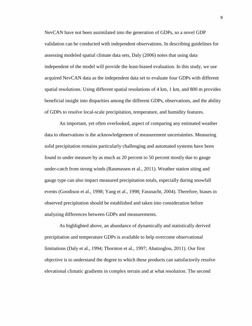
NevCAN have not been assimilated into the generation of GDPs, so a novel GDP

validation can be conducted with independent observations. In describing guidelines for

assessing modeled spatial climate data sets, Daly (2006) notes that using data

independent of the model will provide the least-biased evaluation. In this study, we use

acquired NevCAN data as the independent data set to evaluate four GDPs with different

spatial resolutions. Using different spatial resolutions of 4 km, 1 km, and 800 m provides

beneficial insight into disparities among the different GDPs, observations, and the ability

of GDPs to resolve local-scale precipitation, temperature, and humidity features.

An important, yet often overlooked, aspect of comparing any estimated weather

data to observations is the acknowledgement of measurement uncertainties. Measuring

solid precipitation remains particularly challenging and automated systems have been

found to under measure by as much as 20 percent to 50 percent mostly due to gauge

under-catch from strong winds (Rasmussen et al., 2011). Weather station siting and

gauge type can also impact measured precipitation totals, especially during snowfall

events (Goodison et al., 1998; Yang et al., 1998; Fassnacht, 2004). Therefore, biases in

observed precipitation should be established and taken into consideration before

analyzing differences between GDPs and measurements.

As highlighted above, an abundance of dynamically and statistically derived

precipitation and temperature GDPs is available to help overcome observational

limitations (Daly et al., 1994; Thornton et al., 1997; Abatzoglou, 2011). Our first

objective is to understand the degree to which these products can satisfactorily resolve

elevational climatic gradients in complex terrain and at what resolution. The second

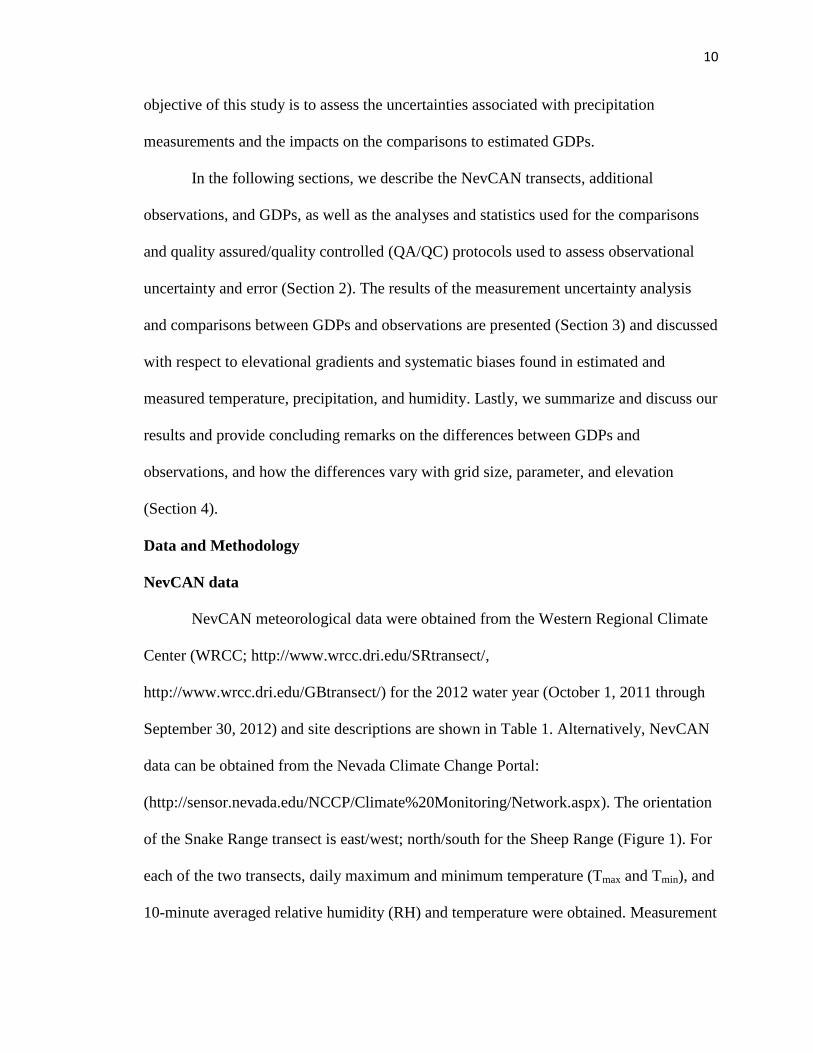
10

objective of this study is to assess the uncertainties associated with precipitation

measurements and the impacts on the comparisons to estimated GDPs.

In the following sections, we describe the NevCAN transects, additional

observations, and GDPs, as well as the analyses and statistics used for the comparisons

and quality assured/quality controlled (QA/QC) protocols used to assess observational

uncertainty and error (Section 2). The results of the measurement uncertainty analysis

and comparisons between GDPs and observations are presented (Section 3) and discussed

with respect to elevational gradients and systematic biases found in estimated and

measured temperature, precipitation, and humidity. Lastly, we summarize and discuss our

results and provide concluding remarks on the differences between GDPs and

observations, and how the differences vary with grid size, parameter, and elevation

(Section 4).

Data and Methodology

NevCAN data

NevCAN meteorological data were obtained from the Western Regional Climate

Center (WRCC; http://www.wrcc.dri.edu/SRtransect/,

http://www.wrcc.dri.edu/GBtransect/) for the 2012 water year (October 1, 2011 through

September 30, 2012) and site descriptions are shown in Table 1. Alternatively, NevCAN

data can be obtained from the Nevada Climate Change Portal:

(http://sensor.nevada.edu/NCCP/Climate%20Monitoring/Network.aspx). The orientation

of the Snake Range transect is east/west; north/south for the Sheep Range (Figure 1). For

each of the two transects, daily maximum and minimum temperature (Tmax and Tmin), and

10-minute averaged relative humidity (RH) and temperature were obtained. Measurement

http://www.wrcc.dri.edu/SRtransect/

http://www.wrcc.dri.edu/GBtransect/

http://sensor.nevada.edu/NCCP/Climate%20Monitoring/Network.aspx

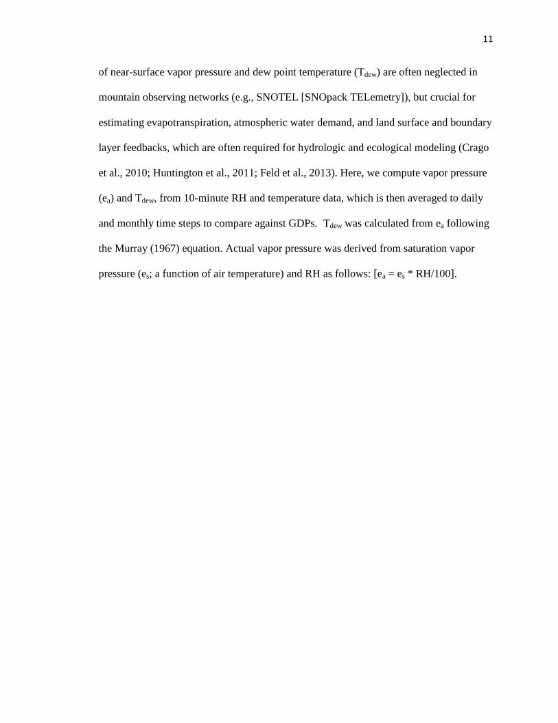
11

of near-surface vapor pressure and dew point temperature (Tdew) are often neglected in

mountain observing networks (e.g., SNOTEL [SNOpack TELemetry]), but crucial for

estimating evapotranspiration, atmospheric water demand, and land surface and boundary

layer feedbacks, which are often required for hydrologic and ecological modeling (Crago

et al., 2010; Huntington et al., 2011; Feld et al., 2013). Here, we compute vapor pressure

(ea) and Tdew, from 10-minute RH and temperature data, which is then averaged to daily

and monthly time steps to compare against GDPs. Tdew was calculated from ea following

the Murray (1967) equation. Actual vapor pressure was derived from saturation vapor

pressure (es; a function of air temperature) and RH as follows: [ea = es * RH/100].

12

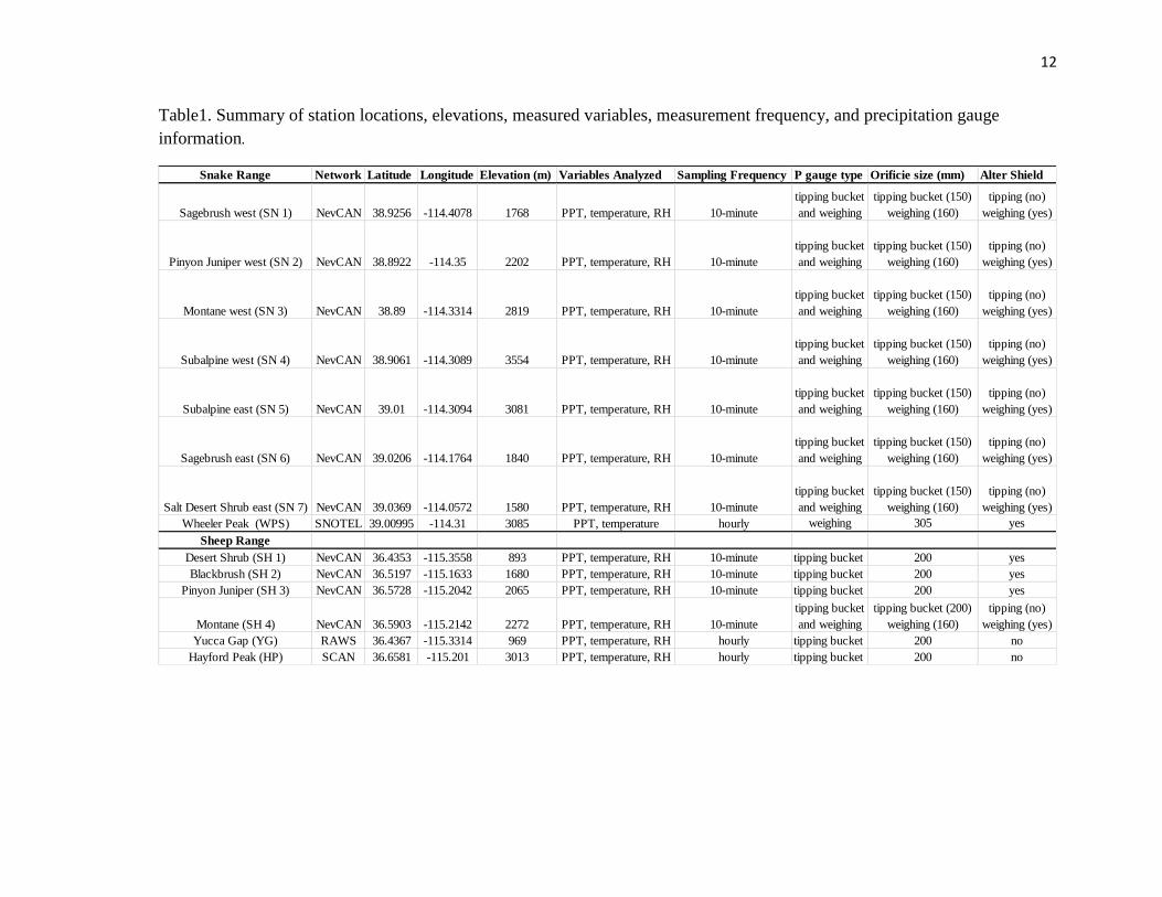
Table1. Summary of station locations, elevations, measured variables, measurement frequency, and precipitation gauge

information.

Snake Range Network Latitude Longitude Elevation (m) Variables Analyzed Sampling Frequency P gauge type Orificie size (mm) Alter Shield

Sagebrush west (SN 1) NevCAN 38.9256 -114.4078 1768 PPT, temperature, RH 10-minute

tipping bucket

and weighing

tipping bucket (150)

weighing (160)

tipping (no)

weighing (yes)

Pinyon Juniper west (SN 2) NevCAN 38.8922 -114.35 2202 PPT, temperature, RH 10-minute

tipping bucket

and weighing


weighing (160)

tipping (no)

weighing (yes)

Montane west (SN 3) NevCAN 38.89 -114.3314 2819 PPT, temperature, RH 10-minute

tipping bucket

and weighing


weighing (160)

tipping (no)

weighing (yes)

Subalpine west (SN 4) NevCAN 38.9061 -114.3089 3554 PPT, temperature, RH 10-minute

tipping bucket

and weighing


weighing (160)

tipping (no)

weighing (yes)

Subalpine east (SN 5) NevCAN 39.01 -114.3094 3081 PPT, temperature, RH 10-minute

tipping bucket

and weighing


weighing (160)

tipping (no)

weighing (yes)

Sagebrush east (SN 6) NevCAN 39.0206 -114.1764 1840 PPT, temperature, RH 10-minute

tipping bucket

and weighing


weighing (160)

tipping (no)

weighing (yes)

Salt Desert Shrub east (SN 7) NevCAN 39.0369 -114.0572 1580 PPT, temperature, RH 10-minute

tipping bucket

and weighing


weighing (160)

tipping (no)

weighing (yes)

Wheeler Peak (WPS) SNOTEL 39.00995 -114.31 3085 PPT, temperature hourly weighing 305 yes

Sheep Range

Desert Shrub (SH 1) NevCAN 36.4353 -115.3558 893 PPT, temperature, RH 10-minute tipping bucket 200 yes

Blackbrush (SH 2) NevCAN 36.5197 -115.1633 1680 PPT, temperature, RH 10-minute tipping bucket 200 yes

Pinyon Juniper (SH 3) NevCAN 36.5728 -115.2042 2065 PPT, temperature, RH 10-minute tipping bucket 200 yes

Montane (SH 4) NevCAN 36.5903 -115.2142 2272 PPT, temperature, RH 10-minute

tipping bucket

and weighing


weighing (160)

tipping (no)

weighing (yes)

Yucca Gap (YG) RAWS 36.4367 -115.3314 969 PPT, temperature, RH hourly tipping bucket 200 no

Hayford Peak (HP) SCAN 36.6581 -115.201 3013 PPT, temperature, RH hourly tipping bucket 200 no

13

Figure 1: (A) Study area with insets indicating locations of the Snake and Sheep Ranges.

Close up of the (B) Snake Range and (C) Sheep Range with red dots indicating station

locations. Zoomed-in frame (B) highlights the close proximity of Wheeler Peak SNOTEL

(WPS) to NevCAN. Station summaries can be found in Table 1.

All observations were QA/QCed by manual inspection to check for erroneous outliers,

and then aggregated to monthly time steps for monthly comparisons of GDP data.

Precipitation can be highly variable over short temporal scales, therefore raw 10-

minute data were summed to the day instead of using the WRCC pre-computed daily

precipitation, as an additional QA/QC measure. At the Snake Range, each station is

equipped with two precipitation gauge systems: (1) a weighing gauge with a 160-mm

14

diameter orifice (Geonor T-200B), and (2) a tipping bucket with a 150-mm diameter

orifice (TE 525). At the Sheep Range, all stations are equipped with tipping buckets

(TB4, 200-mm diameter orifice) except for SH4, which is the only station to have both

types of gauges. At locations with both types of gauges, only the Geonor gauges are

equipped with Alter shields (Alter, 1937) to reduce gauge under-catch, while the tipping

buckets were left unshielded. Alter shields were installed at tipping-bucket-only sites in

the Sheep Range.

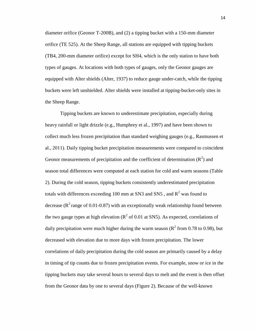
Tipping buckets are known to underestimate precipitation, especially during

heavy rainfall or light drizzle (e.g., Humphrey et al., 1997) and have been shown to

collect much less frozen precipitation than standard weighing gauges (e.g., Rasmussen et

al., 2011). Daily tipping bucket precipitation measurements were compared to coincident

Geonor measurements of precipitation and the coefficient of determination (R2) and

season total differences were computed at each station for cold and warm seasons (Table

2). During the cold season, tipping buckets consistently underestimated precipitation

totals with differences exceeding 100 mm at SN3 and SN5 , and R2 was found to

decrease (R2

range of 0.01-0.87) with an exceptionally weak relationship found between

the two gauge types at high elevation (R2 of 0.01 at SN5). As expected, correlations of

daily precipitation were much higher during the warm season (R2 from 0.78 to 0.98), but

decreased with elevation due to more days with frozen precipitation. The lower

correlations of daily precipitation during the cold season are primarily caused by a delay

in timing of tip counts due to frozen precipitation events. For example, snow or ice in the

tipping buckets may take several hours to several days to melt and the event is then offset

from the Geonor data by one to several days (Figure 2). Because of the well-known

15

limitations of tipping buckets (e.g. Humphrey et al., 1997, Rasmussen et al., 2011), and

as highlighted in this analysis, weighing gauge precipitation measurements were used for

evaluating the skill of GDP precipitation estimates when available.

16

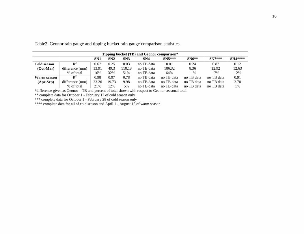
Table2. Geonor rain gauge and tipping bucket rain gauge comparison statistics.

Tipping bucket (TB) and Geonor comparison*

SN1 SN2 SN3 SN4 SN5*** SN6** SN7*** SH4****

Cold season

(Oct-Mar) R

2 0.67 0.25 0.03 no TB data 0.01 0.24 0.87 0.12

difference (mm) 13.91 49.3 118.13 no TB data 186.32 8.36 12.92 12.63

% of total 16% 32% 51% no TB data 64% 11% 17% 12%

Warm season

(Apr-Sep)

R2 0.98 0.97 0.78 no TB data no TB data no TB data no TB data 0.91

difference (mm) 23.26 19.73 9.98 no TB data no TB data no TB data no TB data 2.78

% of total 21% 12% 5% no TB data no TB data no TB data no TB data 1%

*difference given as Geonor – TB and percent of total shown with respect to Geonor seasonal total.

** complete data for October 1 - February 17 of cold season only

*** complete data for October 1 - February 28 of cold season only

**** complete data for all of cold season and April 1 - August 15 of warm season

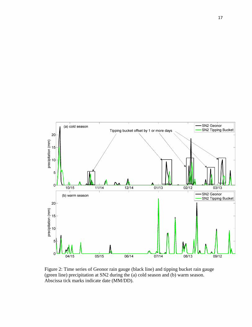
17

Figure 2: Time series of Geonor rain gauge (black line) and tipping bucket rain gauge

(green line) precipitation at SN2 during the (a) cold season and (b) warm season.

Abscissa tick marks indicate date (MM/DD).

18

Additional observations

We use a Natural Resources Conservation Service (NRCS) SNOTEL station

(Tmax, Tmin, and precipitation) to compare to a nearby (~50 m) NevCAN Snake Range

station located in the high-elevation subalpine region and to all GDPs. The Wheeler Peak

SNOTEL (WPS) precipitation gauge is a weighing-type gauge; however the orifice

diameter is approximately twice the size (~305 mm) of the NevCAN Geonors (~160

mm). Daily Tmax, Tmin, and precipitation SNOTEL data were obtained from the NRCS

(http://www.wcc.nrcs.usda.gov/nwcc/site?sitenum=1147&state=nv) and aggregated to

monthly time steps and QA/QCed.

The WPS station is the only high-elevation station in the Snake Range being used

as a control point for PRISM and Daymet spatial distribution algorithms (M. Halbleib,

Oregon State University, electronic communication, http://daymet.ornl.gov/

overview). Therefore, the effect of dependent versus independent observations compared

to GDPs is examined. In this portion of the study, we highlight the importance of

thoroughly understanding GDP control point when using GDP estimates for local climate

assessments. Important assumptions related to weather station and precipitation gauge

footprint, siting and exposure, and sensor limitations/deficiencies are also explored.

Two additional stations were used in the Sheep Range in order to develop a more

complete south-north transect with one station from the NRCS Soil Climate Analysis

Network (SCAN) (Figure 1, Table 1). Hourly RH, temperature, and precipitation data

were downloaded (http://www.wcc.nrcs.usda.gov/scan/) and QA/QCed. The Hayford

Peak (HP) SCAN station is equipped with an unheated tipping bucket and has an eight-

http://www.wcc.nrcs.usda.gov/nwcc/site?sitenum=1147&state=nv

http://www.wcc.nrcs.usda.gov/scan/

19

inch (~200 mm) diameter orifice. Therefore, the winter precipitation data contain large

uncertainties due tipping bucket deficiencies described in Section 2.1. The Yucca Gap

(YG) Remote Automated Weather Station (RAWS) was the second additional station

used at the Sheep Range and hourly RH, temperature, and precipitation data were

downloaded from WRCC (http://www.raws.dri.edu/cgi-bin/rawMAIN.pl?nvNYUC) and

QA/QCed. Yucca Gap is also instrumented with an unheated tipping bucket precipitation

gauge, therefore winter precipitation values are highly uncertain and discussed later. Dew

point and vapor pressure were computed following the same methods used for NevCAN

data. All observations used in the study are summarized in Table 1.

Gridded data

In this study, NevCAN data sets are considered to be “baseline measurements” to

evaluate the skill of four GDPs: (1) PRISM 4-km (Daly et al., 1994), (2) PRISM 800-m

(Daly et al., 1994), (3) Daily Surface Weather and Climatological Summaries (hereafter

called Daymet) 1-km (Thornton et al., 1997), and (4) a North American Land Data

Assimilation (NLDAS)/PRISM hybrid 4-km (hereafter called JA; Abatzoglou, 2011). We

address the uncertainties in NevCAN precipitation measurements and highlight how these

biased observations impact the comparisons to GDPs in the results and discussion

section.

Total monthly PRISM precipitation and average monthly Tmax, Tmin, and Tdew

were obtained (acquisition date: January 2013) for both 800-m and 4-km spatial

resolutions from the PRISM website (www.prism.oregonstate.edu). All variables were

interpolated by PRISM using Climatologically-Aided Interpolation (CAI; Willmott and

Robeson, 1995). For Tmax, Tmin, and precipitation, PRISM was used to interpolate 1971-

http://www.raws.dri.edu/cgi-bin/rawMAIN.pl?nvNYUC

20

2000 monthly normals, using elevation as the predictor grid, with stations weighted by

vertical and horizontal distance, plus several physiographic factors, such as topographic

orientation, coastal proximity, inversion height, and topographic position (Daly et al.,

2008). Once the normals were interpolated, CAI was used to interpolate data for a given

month and year. Average monthly PRISM Tdew estimates were computed by first taking

monthly dew point depression (Ko) observations and spatially interpolating monthly Ko

using PRISM Tmin as the predictor in the regression function. Dew point was then back

calculated using PRISM Ko and Tmin (Chris Daly, Oregon State University, electronic

communication). To create the monthly dew point time series, CAI was again used;

PRISM assimilated station data in the form of monthly mean dew point, and used the

1971-2000 normal dew point for that month as the predictor grid in its local regression

function. The Murray (1967) equation was rearranged and used to compute vapor

pressure, where [ea = exp[(0.0707 * Tdew - 0.49299)/(0.00421 * Tdew + 1)].

The third GDP evaluated was developed by Abatzoglou (2011) and combines the

spatial attributes of monthly PRISM data with daily temporal resolution of the North

American Land Data Assimilation (NLDAS-2; Mitchell et al., 2004). All of the NLDAS-

2 non-precipitation surface variables are derived from the North American Regional

Reanalysis (NARR; Mesinger et al., 2006), and the native NARR data is spatially

downscaled from 32-km to 12-km and temporally disaggregated from 3-hourly to hourly

(Cosgrove et al., 2003). For NLDAS-2 precipitation, Climate Prediction Center (CPC)

gridded daily gauge data (with a PRISM topographical adjustment) are the primary data

source. Daily CPC data are temporally disaggregated to hourly using radar and satellite-

based estimates (if available), and NARR. The first step in developing JA data is a

21

bilinear interpolation of NLDAS-2 onto the PRISM grid (4-km). CAI is then used to bias

correct the daily temperature, humidity, and precipitation data to a given PRISM month

(Abatzoglou, 2011). Daily Tmax, Tmin, RHmax, RHmin, and total precipitation were

obtained from: http://cloud.insideidaho.org/data/epscor/gridmet/. Dew point from JA was

calculated at the daily time step as a function of actual vapor pressure following the

Murray (1967) equation. Actual vapor pressure was derived from RHmax, RHmin,

saturation vapor pressure at Tmax (estmax), and saturation vapor pressure at Tmin (estmin),

where [ea = (estmax * (RHmin/100) + estmin * (RHmax/100)) / 2], as recommended by Allen

et al. (1998) for daily data.

Daymet was the fourth GDP evaluated, and is available for all of North America

at daily time steps and at 1-km spatial resolution. Daily Tmax, Tmin, precipitation, and

vapor pressure data were acquired online (http://daymet.ornl.gov; Thornton et al., 2012).

To interpolate Tmax, Tmin, and precipitation, Daymet uses a truncated Gaussian filter, and

a weighted least-squares regression is applied to establish the relationship between a

given variable and elevation (Thornton et al., 1997). While both Daymet and PRISM use

local linear regression, Daymet assumes a strictly monotonic relationship between

temperature and elevation, which limits the ability of Daymet to handle temperature

inversions (Daly et al., 2006). Daymet daily average vapor pressure is derived following

the assumption that daily Tmin = daily average Tdew (Thornton et al., 1999, 2000).

However, as we show in the results and discussion, Daymet monthly average Tdew rarely

equals Tmin, especially in semiarid and arid environments. Daily average Tdew was

calculated directly from Daymet daily average vapor pressure following Murray (1967).

http://cloud.insideidaho.org/data/epscor/gridmet/

22

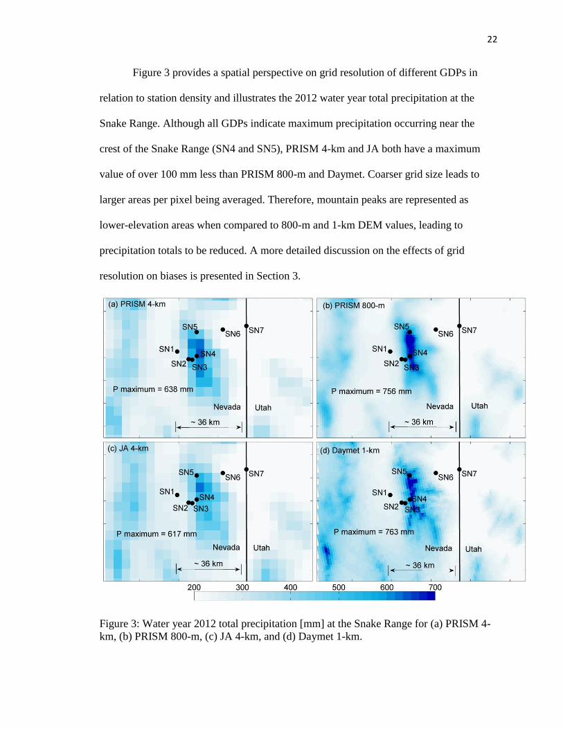
Figure 3 provides a spatial perspective on grid resolution of different GDPs in

relation to station density and illustrates the 2012 water year total precipitation at the

Snake Range. Although all GDPs indicate maximum precipitation occurring near the

crest of the Snake Range (SN4 and SN5), PRISM 4-km and JA both have a maximum

value of over 100 mm less than PRISM 800-m and Daymet. Coarser grid size leads to

larger areas per pixel being averaged. Therefore, mountain peaks are represented as

lower-elevation areas when compared to 800-m and 1-km DEM values, leading to

precipitation totals to be reduced. A more detailed discussion on the effects of grid

resolution on biases is presented in Section 3.

Figure 3: Water year 2012 total precipitation [mm] at the Snake Range for (a) PRISM 4-

km, (b) PRISM 800-m, (c) JA 4-km, and (d) Daymet 1-km.

23

GDP/observation comparison and statistical methods

For each observing station, the nearest GDP center point was found to conduct

direct comparisons for each meteorological variable, as well as elevation (Figure 4).

Given that GDPs largely rely on elevation to distribute climatic variables, differences

between GDP pixel and station elevations were expected to largely explain GDP biases.

For example, Figure 4 shows the PRISM 4-km pixel at SN2 to be more than 200 m

higher than the station elevation. Based on this alone, PRISM 4-km temperature was

expected to be cooler and precipitation was expected to be greater than SN2 observed

values due to environmental lapse rates and typical mid-latitude precipitation-elevation

relationships, where precipitation increases with elevation (Houghton, 1979; Smith, 1979;

Daly et al., 1994). Biases between station observations and GDPs were computed using

seasonal means for Tmax, Tmin, and Tdew and sums for precipitation. Additionally, R2 and

mean absolute error (MAE) was computed using daily means and sums (for JA and

Daymet GDPs). All biases were computed as GDP – observation.

24

Figure 4: Elevation of each station and nearest GDP pixel (a) Snake and (b) Sheep

Ranges. Difference between grid point and station elevation (GDP-station) are shown in

(c) and (d), respectively. X-axis follows the dominant alignment, in the west-to-east

direction for the Snake Range transect and nearly south-to-north for the Sheep Range.

25

Results

Snake Range SN5 and Wheeler Peak SNOTEL intercomparison

An important aspect of any comparison study between estimated and measured

data is an evaluation, or at least an acknowledgement, of the quality of the measured data.

For this study, we compare measured precipitation at the NevCAN SN5 station to

measured precipitation at the Wheeler Peak SNOTEL station (WPS). The distance

between the two stations is ~50 m with an elevation difference of only 3.7 m. Daily and

water year accumulation of precipitation for SN5 and WPS are shown in Figure 5, which

clearly shows that both stations tend to record the same precipitation events; however

WPS consistently has higher daily totals. It seems unrealistic that WPS would receive

~30% more precipitation in one water year than SN5, considering their close proximity

(~50 m apart) and nearly identical elevation.

26

Figure 5: NevCAN SN5 (black) and WPS (magenta) daily precipitation totals (a) and

accumulated precipitation (b) throughout the water year. Abscissa tick marks indicate

date (month-year).

There are a number of factors that could contribute to these contrasting values that

fall within two general categories: (1) instrumentation differences and (2) station siting.

Both gauges are weighing types and have Alter shields and the orifice heights for WPS

and SN5 are 4.9 m and 3 m, respectively, with the WPS orifice diameter being twice that

of SN5 (diameters of 305 mm and 160 mm, respectively). The higher orifice height at

WPS should experience higher wind speed, and therefore less catch when compared to

SN5, which is in contrast to our findings. However, siting characteristics, such as the

27

height of surrounding vegetation and exposure to wind, could also be affecting

precipitation totals, particularly during snowfall events (Goodison et al., 1998; Yang et

al., 1998; Fassnacht, 2004). Photographs from SN5 reveal large, tightly spaced trees

surrounding the shielded Geonor gauge (Figures 6a and 6b), and the gauge height is low

with respect to surrounding tree height, while the tree spacing around the WPS gauge

appears to be much less dense (Figures 6c and 6d). The prevailing wind direction in the

winter months is from the west-southwest, and the clusters of large trees surrounding

SN5 (specifically the clusters to the west of the gauge; Figure 6b) are likely physically

blocking wind-blown snow from being captured in the gauge, whereas less dense forest

lies directly to the west of WPS (not shown, but can be seen from satellite imagery). It

should also be noted that the SNOTEL gauge reports precipitation to the nearest tenth of

an inch, while the Geonors report to the nearest hundredth of an inch, indicating greater

precision in the precipitation that is caught by the NevCAN gauges. Differences in

gauge calibration could also lead to different precipitation measurements for similar

events (Sieck et al., 2007), which may be yet another factor leading to the discrepancies

identified in this section.

Inconsistencies and biases in measurements due to station siting, calibration, and

design are problematic if used for impact assessments and reports. Through the

intercompariosn of SN5 and WPS, we have shown that great uncertainty remains with

respect to precipitation measurements in this region, and the resulting comparisons to

GDPs will also contain a large degree of uncertainty. Unfortunately, a comparison such

as we have presented here is not possible with other NevCAN stations because WPS is

the only SNOTEL in the Snake Range.

28

Figure 6: Photographs of the SN5 Geonor gauge and the surrounding vegetation (a, b).

Photograph (a) was taken looking to the east, and (b) was taken looking to the west.

Photographs of the WPS weighing gauge and surrounding vegetation (c, d). Rain gauges

are highlighted by yellow rectangles. The orientation of (c) and (d) is unknown.

Photographs courtesy of WRCC and NRCS.

Snake Range comparisons of observations and GDPs

Cold season (October through March) and warm season (April through

September) precipitation totals and mean Tmax, Tmin, and Tdew values for station

observations and GDPs over the Snake Range are shown in Figure 7. Typical valley-to-

mountain precipitation gradients were observed with NevCAN measurements and GDP

estimates, with seasonal totals increasing with elevation from west to east, and then

29

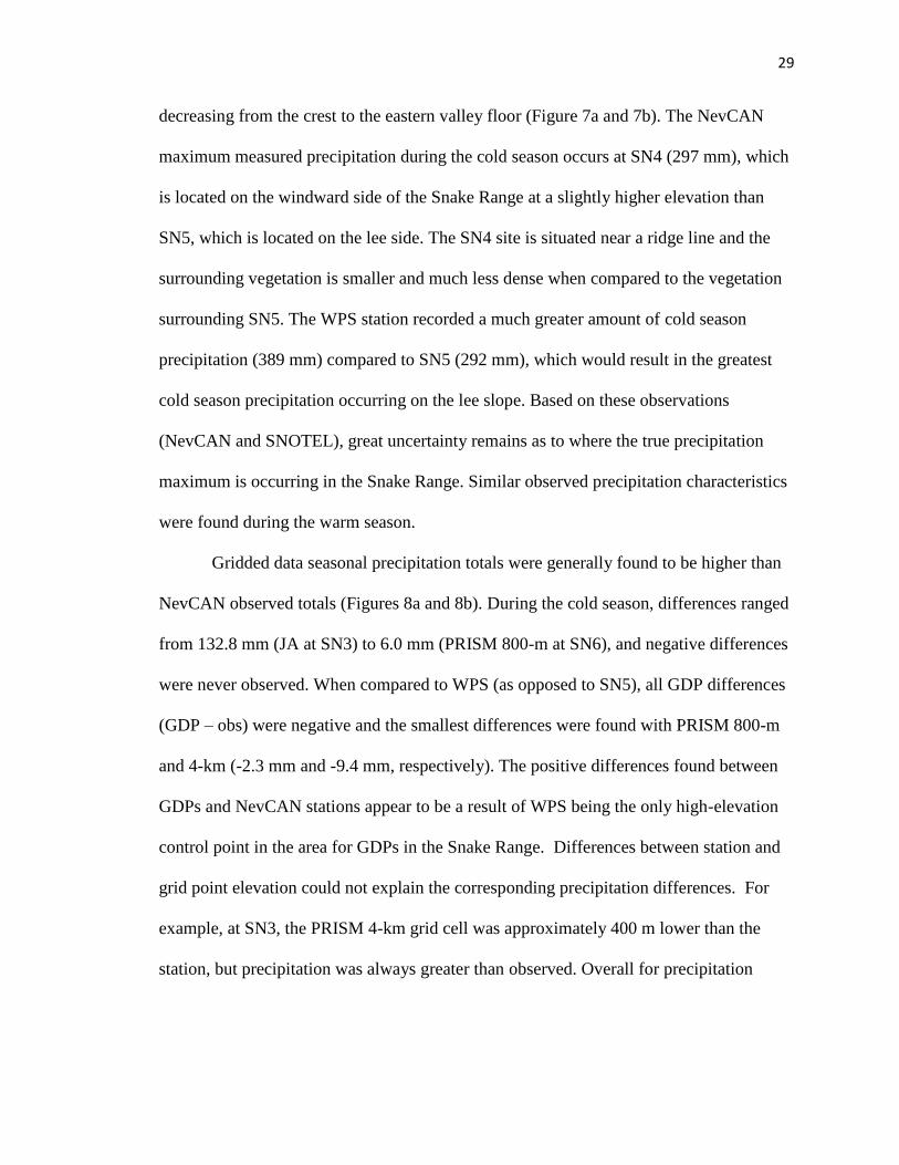
decreasing from the crest to the eastern valley floor (Figure 7a and 7b). The NevCAN

maximum measured precipitation during the cold season occurs at SN4 (297 mm), which

is located on the windward side of the Snake Range at a slightly higher elevation than

SN5, which is located on the lee side. The SN4 site is situated near a ridge line and the

surrounding vegetation is smaller and much less dense when compared to the vegetation

surrounding SN5. The WPS station recorded a much greater amount of cold season

precipitation (389 mm) compared to SN5 (292 mm), which would result in the greatest

cold season precipitation occurring on the lee slope. Based on these observations

(NevCAN and SNOTEL), great uncertainty remains as to where the true precipitation

maximum is occurring in the Snake Range. Similar observed precipitation characteristics

were found during the warm season.

Gridded data seasonal precipitation totals were generally found to be higher than

NevCAN observed totals (Figures 8a and 8b). During the cold season, differences ranged

from 132.8 mm (JA at SN3) to 6.0 mm (PRISM 800-m at SN6), and negative differences

were never observed. When compared to WPS (as opposed to SN5), all GDP differences

(GDP – obs) were negative and the smallest differences were found with PRISM 800-m

and 4-km (-2.3 mm and -9.4 mm, respectively). The positive differences found between

GDPs and NevCAN stations appear to be a result of WPS being the only high-elevation

control point in the area for GDPs in the Snake Range. Differences between station and

grid point elevation could not explain the corresponding precipitation differences. For

example, at SN3, the PRISM 4-km grid cell was approximately 400 m lower than the

station, but precipitation was always greater than observed. Overall for precipitation

30

comparisons, GDP performance was inconsistent, and it was found that finer grid

resolution did not always lead to smaller differences between GDPs and observations.

Maximum temperature biases (Figure 8c and 8d) ranged from 4.9 °C (JA) to -4.6

°C (PRISM 4-km) for cold and warm seasons. Large negative biases (colder than

observed) were found at the low-elevation sites of SN1 and SN2. These biases are

directly related to differences between GDP and station elevations, with SN1 and SN2

grid point elevations being higher than station elevations. However, several GDP

elevations were higher than station elevations leading to positive biases (warmer), and

lower grid point elevations relative to the station elevations with negative biases. For

example, the PRISM 4-km grid point at SN5 is 151 m higher than the SN5 station

elevation and a positive bias of 3.6 °C was found during the cold season.

NevCAN minimum temperature elevational gradients (Figure 7e and 7f) varied

from those of Tmax in that the two alluvial fan “foothill” stations (SN2 and SN6) were

warmer on average when compared to the neighboring valley floor stations (SN1 and

SN7) during both seasons. Previous studies have found that in complex terrain, Tmin can

vary greatly depending on station siting and associated local atmospheric decoupling and

cold-air drainage (Daly et al., 2009; Holden et al., 2011). During the nighttime hours, as

the boundary layer stabilizes (typically during clear sky conditions), cold air sinks and

tends to pool in low-lying areas, leading to temperature inversions near the surface and

warmer conditions in foothill locations (Gustavsson et al., 1998). The ability of GDPs to

capture this feature was variable, with PRISM 800-m being only GDP to capture the

inversions at SN2 and SN6 during both seasons, which is a result of PRISM’s use of

inversion height, topographic position and varying slopes with elevation (Daly et al.,

31

2008). In some instances, PRISM 4-km and JA were able to represent inversions, but the

magnitudes were much smaller than observed. These results highlight the need for

improved methods of interpolating Tmin observations over complex terrain.

Biases in Tmin (Figure 8e and 8f) ranged from 3.1 °C (JA) to -4.7 °C (PRISM 4-

km), with biases being generally slightly larger during the warm season. Although some

of the biases can be attributed to grid point and respective station elevation differences,

the large Tmin biases at SN2 and SN6 are a result of GDPs not being able to replicate the

inversion strength between valley floor and alluvial fan locations. Local lapse rates of

monthly Tmin (not shown) between SN1 and SN2, and between SN7 and SN6 averaged

over the water year were +7.6 °C/km and +9.4 °C/km, respectively, and were largely

underestimated by GDPs (PRISM 800-m was the closest to observations with water year

average Tmin lapse rates of +5.1 °C/km from SN1 to SN2 and +1.9°C/km from SN7 to

SN6).

With a general lack of humidity observations, relatively little is known about the spatial

behavior of near-surface humidity over complex terrain and the skill of GDPs to estimate

humidity. As expected, we found NevCAN station seasonal average Tdew to decrease with

elevation (Figure 7g and 7h). Except for Daymet, differences between GDP and observed

Tdew were generally small during the cold season (Figures 7g and 8g) and ranged from -

2.3 °C to 1.2 °C, whereas warm season biases (Figures 7h and 8h) were larger and

primarily negative, ranging from -4.7 °C to 0.5 °C. All GDPs, except for Daymet,

showed the same trends with elevation. Daymet estimated nearly constant Tdew with

respect to elevation during the cold season (Figure 7g) and increasing Tdew with elevation

during the warm season (Figure 7h). The lack of skill shown by Daymet is primarily due

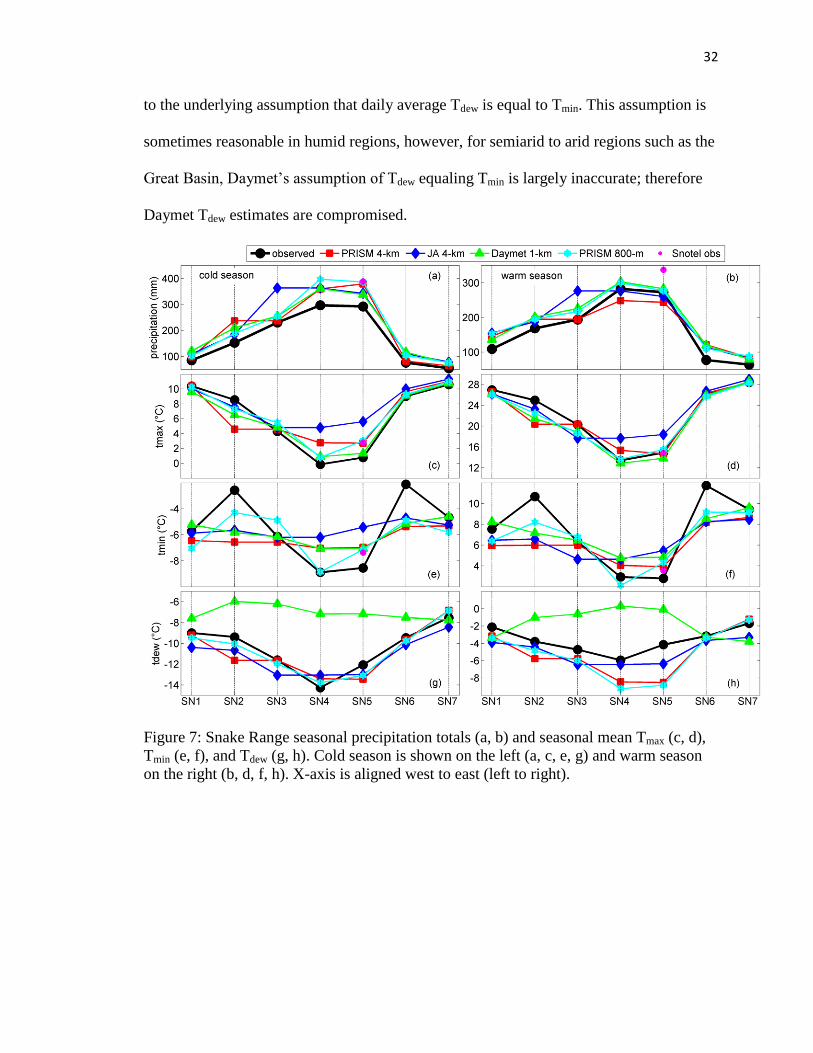
32

to the underlying assumption that daily average Tdew is equal to Tmin. This assumption is

sometimes reasonable in humid regions, however, for semiarid to arid regions such as the

Great Basin, Daymet’s assumption of Tdew equaling Tmin is largely inaccurate; therefore

Daymet Tdew estimates are compromised.

Figure 7: Snake Range seasonal precipitation totals (a, b) and seasonal mean Tmax (c, d),


on the right (b, d, f, h). X-axis is aligned west to east (left to right).

33

Figure 8: Snake Range seasonal bias (GDP - obs) for cold season (left) and warm season

(right) precipitation (a, b), Tmax (c, d), Tmin (e, f), and Tdew (g, h). Variables needed to

calculate Tdew are not measured at WPS, therefore no Tdew values are shown.

To examine the ability of daily GDPs to capture measured daily variability of

temperature and precipitation, R2 and MAE were computed for cold and warm seasons

using Daymet and JA GDPs (Figures 9 and 10). Fairly good agreement was found

between measured and estimated precipitation events during the cold season (Figures 9a

and 9b), with JA consistently having higher R2

(0.68-0.80) and smaller MAE (58%-98%)

when compared to Daymet (R2: 0.41-0.71, MAE: 65%-114%). Contrasting results were

found with warm season precipitation (Figure 10a and 10b); with generally much lower

correlations, and higher MAE. Gridded data appear to be generating more daily misses

34

(GDP = 0, and observed > 0) and false alarms (GDP > 0, and observed = 0) during the

late spring and summer months (not shown). The nature of warm season precipitation

events is typically convective and associated with a monsoonal pattern, which leads to a

sporadic and non-uniform spatial distribution and lower correlations between GDPs and

observations.

Daymet showed higher R2 and lower MAE for Tmax (Figures 9c, 9d, 10c, and 10d)

and Tmin (Figures 9e, 9f, 10e, and 10f) at most locations; however, differences between

JA and Daymet error statistics were often times marginal. In general, higher MAE values

were found with Tmin, which is consistent with our seasonal results that highlight the

weakness in GPDs to simulate inversion strength. The downscaling of the 32-km NARR

temperature data to the 12-km NLDAS-grid, and finally to the 4-km JA grid is likely

leading to lager error when compared to Daymet, where observations are interpolated

directly to a 1-km grid. Not surprisingly, JA Tdew correlations were higher, and MAE was

lower than Daymet, especially during the warm season (Figures 9g, 9h, 10g, and 10h).

This is largely a reflection of the assumptions used in the Daymet algorithm (Tmin equals

Tdew). It should be noted that the calculation of Tdew from daily data with JA and Daymet

is a contributing source of error when compared to NevCAN Tdew that was computed

with 10-minute data. Large differences were found at the daily time step when

comparing NevCAN Tdew from 10-minute data to Tdew from daily data, and differences

often times exceeded 3 °C/day (not shown).

35

Figure 9: Snake Range cold season R2 (left) and MAE (right) computed at the daily time


For precipitation, MAE is expressed as a percentage, while MAE for Tmax, Tmin, and Tdew

is expressed in °C.

36

Figure 10: Snake Range warm season R2 (left) and MAE (right) computed at the daily



Tdew is expressed in °C.

Sheep Range comparisons of observations and GDPs

As discussed in Section 2.1, tipping buckets largely undermeasure precipitation

during the cold season, and therefore Sheep Range tipping bucket measurements (Table

1, Figure 11a and 11b) must be considered inaccurate at the daily time step (and biased

low). Unfortunately, all Sheep Range stations are equipped with tipping buckets only,

except for SH4. Based on the assumption that frozen precipitation will occur at

temperatures of less than 0 °C, SH1 and YG were the only stations where all precipitation

37

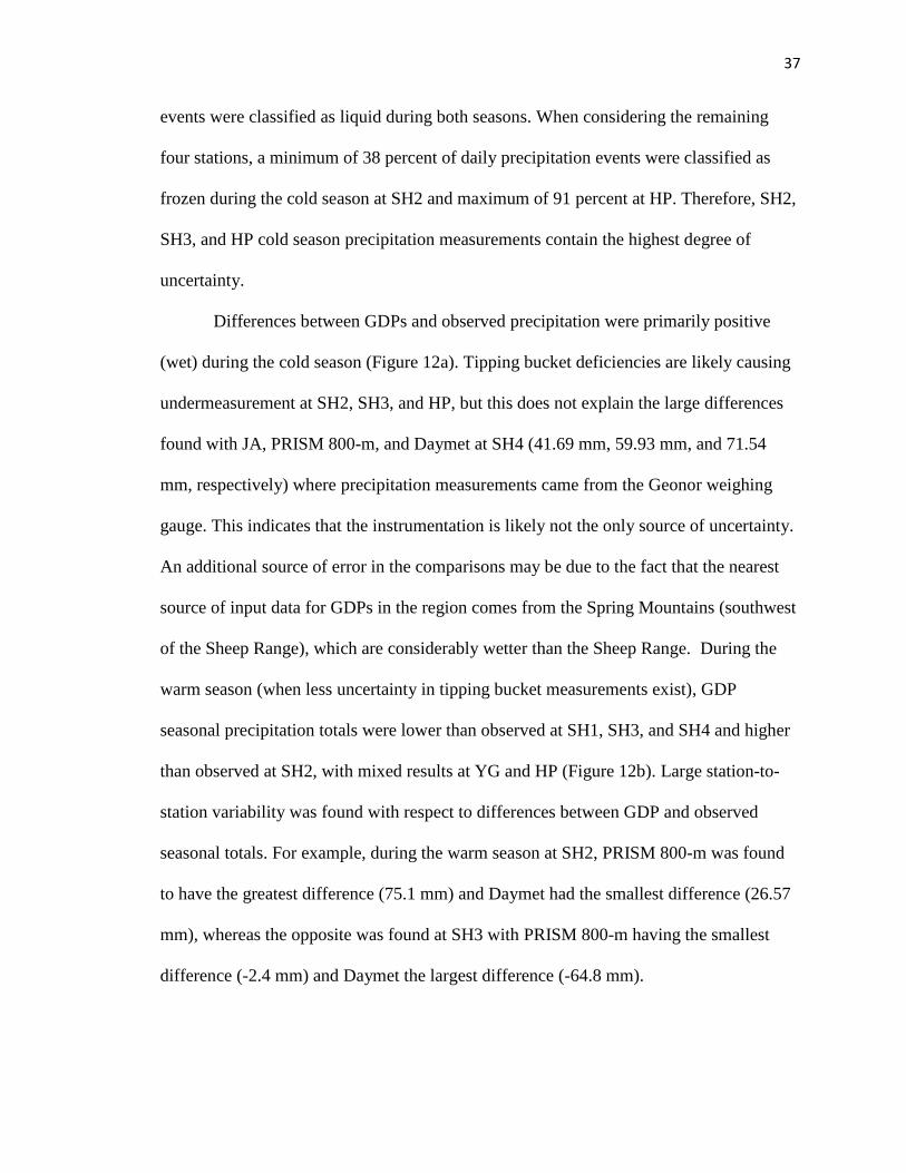
events were classified as liquid during both seasons. When considering the remaining

four stations, a minimum of 38 percent of daily precipitation events were classified as

frozen during the cold season at SH2 and maximum of 91 percent at HP. Therefore, SH2,

SH3, and HP cold season precipitation measurements contain the highest degree of

uncertainty.

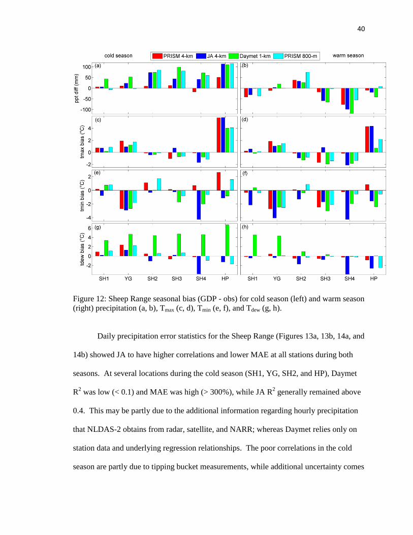
Differences between GDPs and observed precipitation were primarily positive

(wet) during the cold season (Figure 12a). Tipping bucket deficiencies are likely causing

undermeasurement at SH2, SH3, and HP, but this does not explain the large differences

found with JA, PRISM 800-m, and Daymet at SH4 (41.69 mm, 59.93 mm, and 71.54

mm, respectively) where precipitation measurements came from the Geonor weighing

gauge. This indicates that the instrumentation is likely not the only source of uncertainty.

An additional source of error in the comparisons may be due to the fact that the nearest

source of input data for GDPs in the region comes from the Spring Mountains (southwest

of the Sheep Range), which are considerably wetter than the Sheep Range. During the

warm season (when less uncertainty in tipping bucket measurements exist), GDP

seasonal precipitation totals were lower than observed at SH1, SH3, and SH4 and higher

than observed at SH2, with mixed results at YG and HP (Figure 12b). Large station-to-

station variability was found with respect to differences between GDP and observed

seasonal totals. For example, during the warm season at SH2, PRISM 800-m was found

to have the greatest difference (75.1 mm) and Daymet had the smallest difference (26.57

mm), whereas the opposite was found at SH3 with PRISM 800-m having the smallest

difference (-2.4 mm) and Daymet the largest difference (-64.8 mm).

38

Maximum temperature biases during the cold season (Figure 12c) ranged from -

1.67 °C (JA) to 5.77 °C (JA) and from -2.11 °C (JA) to 4.33 °C (JA) during the warm

season (Figure 12d). The consistently large warm biases found at HP can be primarily

explained by the large differences found between GDP and station elevations, with GDP

elevations being -88 m to -422 mm lower than the HP station elevation.

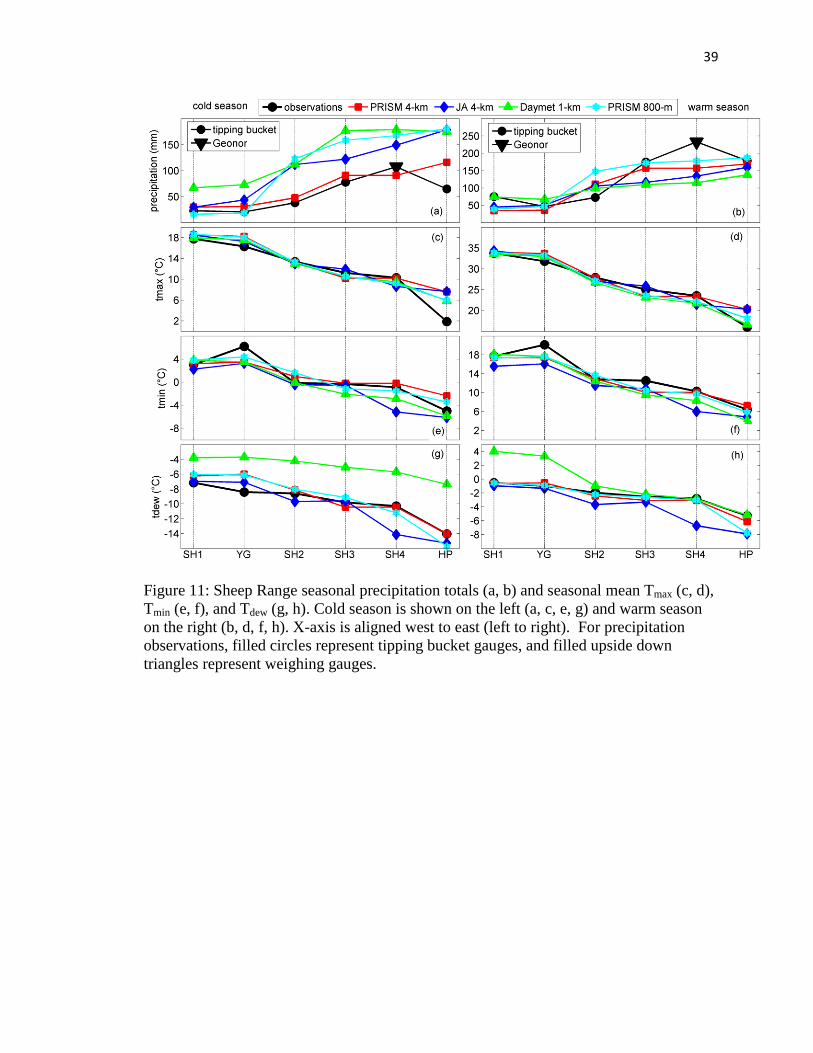
Observed seasonal mean Tmin (Figure 11e and 11f) was found to have similar

characteristics as the Snake Range, with the alluvial fan station (YG) being warmer than

the lower-elevation valley floor station (SH1) during both seasons. Daymet was the only

GDP to not capture the cold air drainage feature. This highlights the importance of

accounting for complex, non-monotonic elevational gradients and temperature inversions,

which are common throughout the Great Basin. Seasonal mean Tmin biases during the

cold season (Figure 12e) ranged from

-4.28 °C (JA) to 2.64 °C (PRISM 4-km) and from -4.26 °C (JA) to 0.88 °C (PRISM 800-

m) during the warm season (Figure 12f). As found at the Snake Range, Tmin biases are not

directly related to differences between GDP and station elevations. For example, cold

biases were found at HP with JA and Daymet during both seasons although the GDP

elevations were lower than the station elevation (-335 m and -88 m, respectively).

Both observed and GDP estimated seasonal mean Tdew was found to decrease with

elevation (Figures 11g and 11h). This is in contrast to the Snake Range, where Daymet

Tdew was found to increase with elevation during the warm season. Little consistency was

found in GDP seasonal mean Tdew biases (Figures 12g and 12h), with the exception of

Daymet showing a consistent and large positive (warm) bias during the cold season,

ranging from 3.42 °C to 6.63 °C.

39

Figure 11: Sheep Range seasonal precipitation totals (a, b) and seasonal mean Tmax (c, d),


on the right (b, d, f, h). X-axis is aligned west to east (left to right). For precipitation

observations, filled circles represent tipping bucket gauges, and filled upside down

triangles represent weighing gauges.

40

Figure 12: Sheep Range seasonal bias (GDP - obs) for cold season (left) and warm season

(right) precipitation (a, b), Tmax (c, d), Tmin (e, f), and Tdew (g, h).

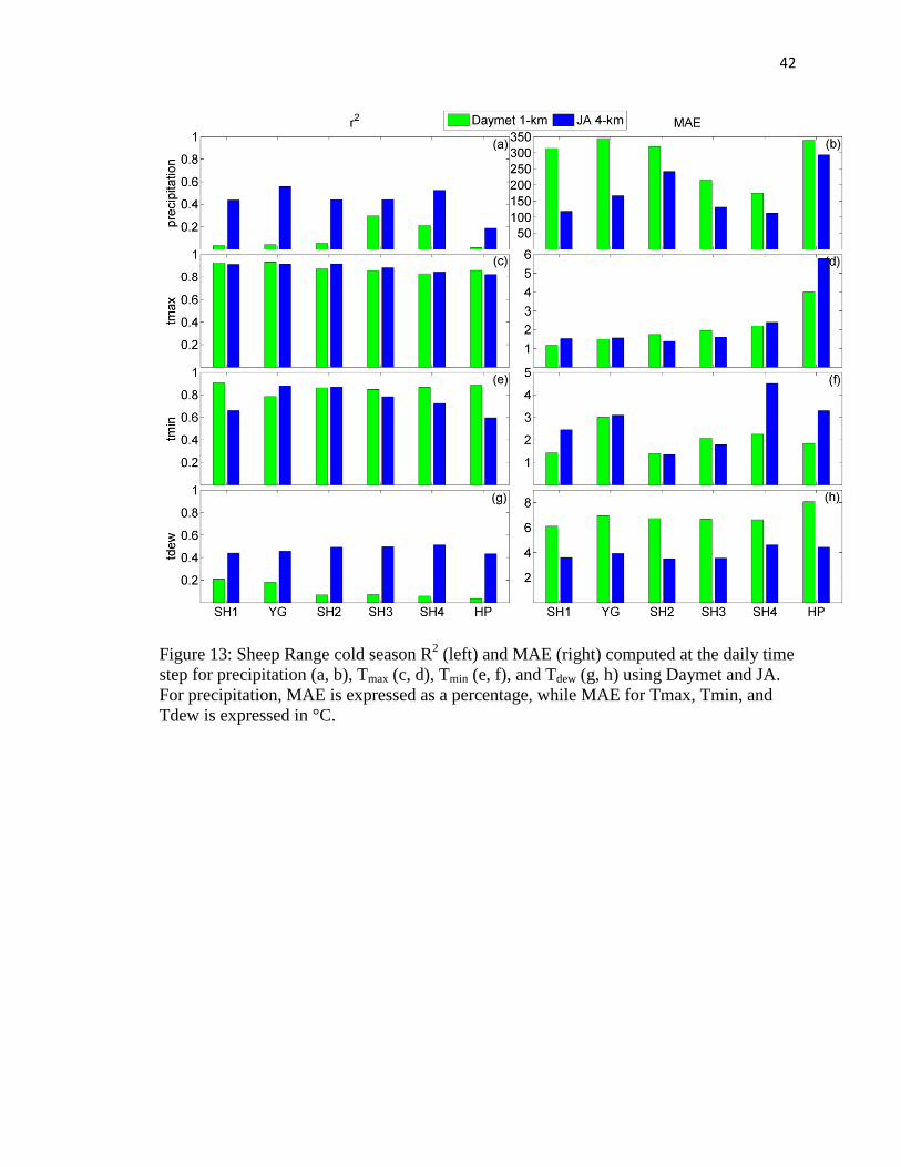
Daily precipitation error statistics for the Sheep Range (Figures 13a, 13b, 14a, and

14b) showed JA to have higher correlations and lower MAE at all stations during both

seasons. At several locations during the cold season (SH1, YG, SH2, and HP), Daymet

R2 was low (< 0.1) and MAE was high (> 300%), while JA R

2 generally remained above

0.4. This may be partly due to the additional information regarding hourly precipitation

that NLDAS-2 obtains from radar, satellite, and NARR; whereas Daymet relies only on

station data and underlying regression relationships. The poor correlations in the cold

season are partly due to tipping bucket measurements, while additional uncertainty comes

41

from a lack of GDP station data input in this region. It should also be noted that in this

arid climate, precipitation occurs on only a small fraction of days (i.e. an average of 13%

of days in the cold season), so correlations will decrease rapidly for each day that GDPs

don’t match observed precipitation. The combination of no GDP input from surface

observations in the Sheep range, and primarily tipping bucket rain gauges, leads to great

uncertainty in both GDP estimates and NevCAN observations of precipitation in the

Sheep Range.

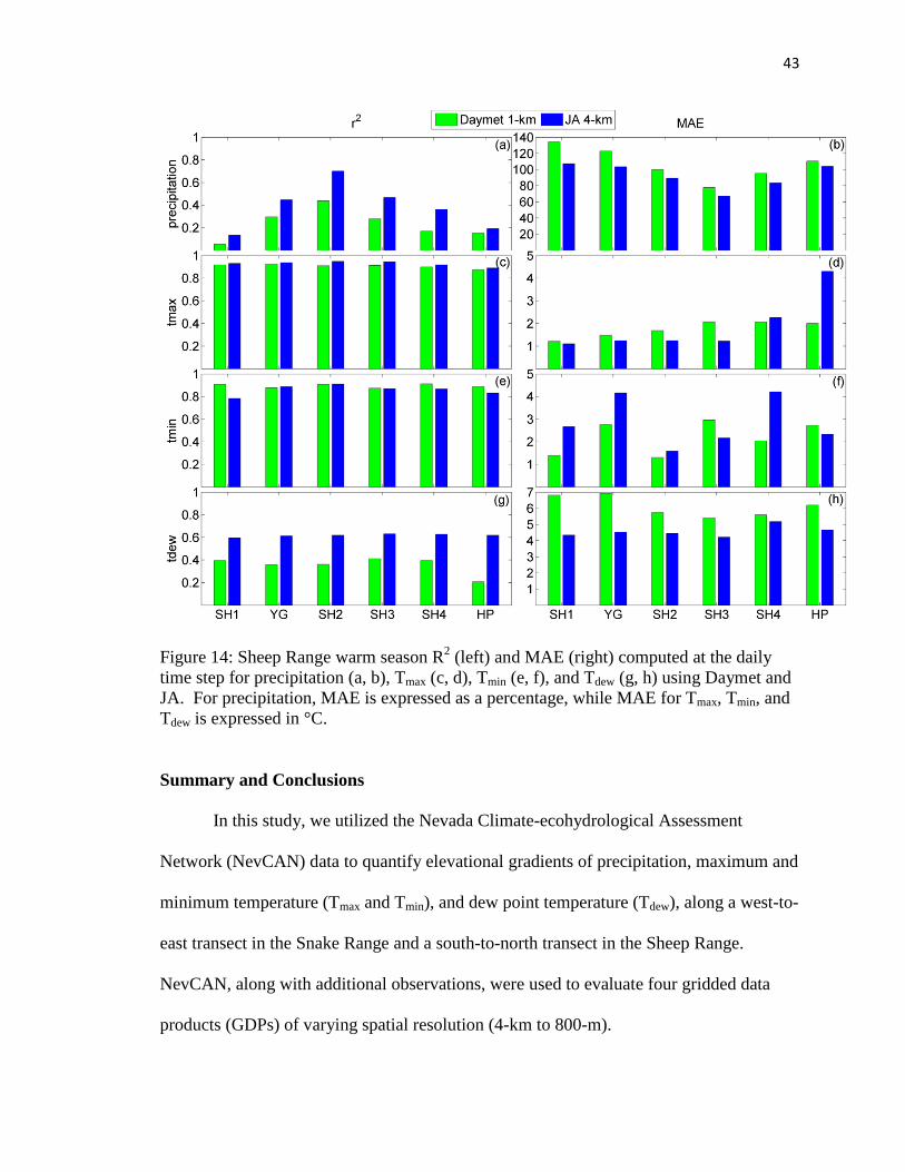
Daymet and JA Tmax correlations (Figures 13c and 14c) were quite similar and

indicate good agreement to observations (R2 always > 0.82), and the noticeably higher

MAE at HP (Figures 13d and 14d) could be attributed to the large differences between

grid cell and station elevation. For Tmin, error statistics were generally still good, but

lower than Tmax, which is again due to GDP errors with inversions. Daily Tdew error

statistics (Figures 13g, 13h, 14g, and 14h) were consistent with the Snake Range, with JA

always indicating less error than Daymet due to previously described deficiencies.

42

Figure 13: Sheep Range cold season R2 (left) and MAE (right) computed at the daily time


For precipitation, MAE is expressed as a percentage, while MAE for Tmax, Tmin, and


43

Figure 14: Sheep Range warm season R2 (left) and MAE (right) computed at the daily




Summary and Conclusions

In this study, we utilized the Nevada Climate-ecohydrological Assessment

Network (NevCAN) data to quantify elevational gradients of precipitation, maximum and

minimum temperature (Tmax and Tmin), and dew point temperature (Tdew), along a west-to-

east transect in the Snake Range and a south-to-north transect in the Sheep Range.

NevCAN, along with additional observations, were used to evaluate four gridded data

products (GDPs) of varying spatial resolution (4-km to 800-m).

44

We have highlighted the challenges of providing reliable “ground truth” for

evaluating GDP precipitation estimates in remote areas. By identifying large differences

in water year (2012) precipitation totals between SN5 and the Wheeler Peak SNOTEL

(WPS) station (161 mm) and through the comparison of tipping bucket and weighing

gauge measurements presented in Section 3.1, we have highlighted several difficulties

associated with comparing measurements of precipitation to GDP estimates of

precipitation. The high GDP totals that were found with respect to NevCAN totals may

largely be due to WPS being the only GDP input in the Snake Range. At the Sheep

Range, perceived GDP “overestimation” is partly due to the use of tipping bucket rain

gauges as the source of baseline NevCAN measurements used for comparison. A second

contribution to the large differences between GDPs and Sheep Range observed

precipitation is due to lack of any stations in the Sheep Range being used as GDP input.

Potential users of gridded precipitation data should be aware that large uncertainty exists

where station density is low, and especially when considering small, remote mountain

ranges with no observations used as GDP input (such as the Sheep Range). It is highly

recommend that any observing network with automated precipitation measurements be

equipped with weighing-type gauges and wind shields, as this work and previous studies

(e.g., Humphrey et al., 1997, Rasmussen et al., 2011) have noted large errors associated

with tipping bucket measurements.

A key finding of this study was that temperature inversions at the alluvial fan

locations were identified at both NevCAN transects, highlighting the importance of

mountain transect observation networks. These findings are consistent with previous

research that has identified cold air drainage as being the cause of this inverted Tmin-

45

elevation relationship (Gustavsson et al., 1998; Daly et al., 2009; Holden et al., 2011).

The only GDP not able to replicate this temperature feature was Daymet; however, the

magnitude of the Tmin inversions observed at the Snake Range (mean monthly lapse rates

of > +15°C/km in some cases) was not estimated well by any GDP. Both Daymet and

PRISM use local linear regressions of climate and elevation. However, the slope of the

PRISM regression line can vary sharply with elevation, based on local inversion height

and topographic position information. In contrast, the Daymet regression function is

monotonic through the entire elevation range (Daly, 2006). Lack of realistic Tmin in GDPs

was one motivation for development of the new data set, Topography Weather (TopoWx;

Olyer et al. 2014), that uses satellite based land surface temperature as a predictor for

Tmax and Tmin.

Given that maximum temperature showed a strong relationship with elevation,

biases between GDPs and observations were strongly related to differences between GDP

and station elevation. In general, PRISM 800-m and Daymet contained smaller biases

than PRISM 4-km and JA for both Tmax and Tmin, indicating that spatial resolution of less

than 4 km can provide valuable details regarding temperature features.

We have highlighted a limitation of using an overly simplistic estimation for Tdew

(Tmin = daily average Tdew) in semi-arid to arid environments, which results in an

unrealistic increase of Tdew with elevation in the Snake Range and generally a large bias

compared to observations of Tdew. The combination of Daymet’s assumption of Tmin =

daily average Tdew and the inability to reproduce temperature inversions make the

application of Daymet to estimate humidity levels in semi-arid and arid areas largely

uncertain. Reasonable Tdew estimates were provided by PRISM and JA. However, the

46

calculation of Tdew from JA and Daymet daily data was a contributing source of error

when comparing these estimates to NevCAN Tdew, which was computed with 10-minute

data.

This research highlights the importance of conducting local analyses of

observations and potential measurement errors to gain an understanding of potential GDP

biases prior to use in hydro-climatic applications. Although local results may vary, this

work complements other hydro-climatic studies throughout the Great Basin region where

geographical attributes are similar to the NevCAN transects. Procedures and results from

this study are useful for improving our understanding of GDP evaluation and analyses

related to hydro-climatic assessments in semi-arid and arid climates.

Acknowledgements

The authors would like to thank three anonymous reviewers for helping to improve this

manuscript through constructive feedback. We would also like to acknowledge Greg

McCurdy, Dr. Lynn Fenstermaker, Brad Lyles, and Dr. Jay Arnone for their valuable

contributions regarding the NevCAN instrumentation and site characteristics. This work

was partially funded by National Science Foundation under grant number EPS-0814372

and by the Desert Research Institute Divisions of Atmospheric Science and Hydrologic

Science faculty and graduate research. The work was also funded by Landsat Science

Team funding under USGS grant number G12PC00068 and the U.S. Bureau of

Reclamation Nevada Water Resources Evaluation Program in collaboration with the

Nevada State Engineer’s Office, funded by a grant under Public Law 109-103, Section

208(a), Cooperative Agreement 06FC204044.

47

References

Abatzoglou, J. T., 2011: Development of gridded surface meteorological data for

ecological

applications and modeling. Int. J. Climatol. 33, 121–131, DOI: 10.1002/joc.3413.

Ackerly, D. D., S. R. Loarie, W. K. Cornwell, S. B. Weiss, H. Hamilton, R. Branciforte,

and N. J. B. Kraft, 2010: The geography of climate change: implications for

conservation biogeography. Diversity Distrib., 16, 476-487.

Allen, R. G., L. S. Pereira, D. Raes, and M. Smith, 1998: Crop evapotranspiration,

guidelines for

computing crop water requirement. FAO Irrig. and Drain. Paper 56, Food and

Agricultural

Organization of the United Nations. Rome, Italy. 300.

Alter, J. C., 1937: Shielded storage precipitation gages. Mon. Wea. Rev., 65, No. 7, 262-

265.

Bandyopadhyay, J. et al., 1997: Highland waters – a resource of global significance. In:

Messerli, B. and Ives, J. D. (eds.) Mountains of the world – a global priority.

NewYork and London: Parthenon, pp. 131-155.

Barnett, T. P., J. C. Adam, and D. P. Lettenmaier, 2005: Potential impacts of a warming

climate on water availability in snow-dominated regions. Nature, 438, 303-309.

Bradley, B. A., 2009: Regional analysis of the impacts of climate change on cheatgrass

invasion shows potential risk and opportunity. Glob. Change Biol., 15, 196-208, doi:

10.1111/j.1365-2486.2008.01709.x.

48

Burns, A. G. and W. Drici, 2011: Hydrology and water resources of Spring, Cave, Dry

Lake, and

Delamar Valleys, Nevada and vicinity. Presentation to the Office of the Nevada State

Engineer: Southern Nevada Water Authority, Las Vegas, Nevada.

Crago, R. D., R. J. Qualls, and M. Feller, 2010: A calibrated advection-aridity

evaporation model requiring no humidity data, Water Resour. Res., 46, W09519,

doi:10.1029/2009WR008497.

Cosgrove, B. A., and Coauthors, 2003: Real-time and retrospective forcing in the North

American Land Data Assimilation System (NLDAS) project. J. Geophys. Res., 108,

doi:10.1029/2002JD003118.

Daly, C., R. P. Neilson, and D. L. Phillips, 1994: A statistical-topographic model for

mapping

climatological precipitation over mountainous terrain. J. Appl. Meteor., 33, 140-158.

——, 2006: Guidelines for assessing the suitability of spatial climate data sets. Int. J.

Climatol., 26, 707-721.

——, M. Halbleib, J. I. Smith, W. P. Gibson, M. K. Doggett, G. H. Taylor, J. Curtis, and

P. P. Pasteris, 2008: Physiographically sensitive mapping of climatological

temperature and precipitation across the conterminous United States. Int. J. Climatol.,

doi: 10.1002/joc.1688.

——, C., D. R. Conklin, and M. H. Unsworth, 2009. Local atmospheric decoupling in

complex topography alters climate change impacts. Int. J. Climatol., DOI:

10.1002/joc.2007.

Eakin, T. E., 1966: A regional interbasin ground-water system in the White River area,

49

southeastern Nevada, Water Resour. Res, 2, no. 2, 251-271.

Epstein, B. J., G. M., Pohll, J. L. Huntington, R. H. Carrol, 2010: Development and

uncertainty analysis of an empirical recharge prediction model for Nevada’s Desert

Basins. Journal of the Nevada Water Resources Association. 5:1, 1-22. Available at:

http://www.dri.edu/images/stories/divisions/dhs/dhsfaculty/Justin-

Huntington/Epstein_et_al_2010.pdf.

Fassnacht, S. R., 2004: Estimating Alter-shielded gauge snowfall undercatch, snowpack

sublimation, and blowing snow transport at six sites in the coterminous USA. Hydrol.

Process., 18, 3481-3492.

Feld, S. I., N. C. Cristea, and J. D. Lundquist, 2013: Representing atmospheric moisture

content along mountain slopes: examination using distributed sensors in the Sierra

Nevada, California. Water Resour. Res., 49, 4424-4441, doi:10.1002/wrcr.20318.

Flint, A. L., Flint, L. E., Hevesi, J. A., and Blainey, J. M., 2004: Fundamental concepts of

recharge in the Desert Southwest: A regional modeling perspective, in Hogan, J.F.,

Phillips, FM., and Scanlon, B.R., eds., Ground-Water Recharge in a Desert

Environment: The Southwestern United States: American Geophysical Union, Water

Science and Application Series 9, 159-184.

Goodison, B. E., P. Y. T. Louie, and D. Yang, 1998: WMO solid precipitation

measurement intercomparison. WMO Instruments and Observing Methods Report

No. 67, WMO/TD No. 872.

Gustavsson, T., M. Karlsson, J. Bogren, and S. Lindqvist, 1998: Development of

temperature patterns during clear nights. J. Appl. Meteor., 37, 559-571.

http://www.dri.edu/images/stories/divisions/dhs/dhsfaculty/Justin-Huntington/Epstein_et_al_2010.pdf

http://www.dri.edu/images/stories/divisions/dhs/dhsfaculty/Justin-Huntington/Epstein_et_al_2010.pdf

50

Holden, Z. A., J. T. Abatzoglou, L. S. Baggett, and C. Luce, 2011: Empirical

downscaling of daily minimum air temperature at very fine resolutions in complex

terrain. Agr. Forest Meteorol., doi: 10.1016/j.agrformet.2011.03.01.

Houghton, J. G., 1979: A model for orographic precipitation in the north-central Great

Basin. Mon. Wea. Rev., 107, 1462-1475.

Humphrey, M. D., J. D. Istok, J. Y. Lee, A. Hevesi, and A. L. Flint, 1997: A new method

for automated dynamic calibration of tipping-bucket rain gauges. J. Atmos. Ocean.

Tech., 14, 1513-1519.

Huntington, J. L., and D. J. McEvoy, 2011: Climatological estimates of open water

evaporation from selected Truckee and Carson River basin water bodies, California

and Nevada. Desert Research Institute Publication No. 41254. Available at:

http://www.dri.edu/images/stories/divisions/dhs/dhsfaculty/Justin-

Huntington/Huntington_and_McEvoy_2011.pdf

——, J. L. Szilagyi, S. W. Tyler, and G. M. Pohll, 2011: Evaluating the complementary

relationship for estimating evapotranspiration from arid shrublands, Water Resour.

Res., doi:10.1029/2010WR009874.

——, and R. G. Niswonger, 2012: Role of surface-water and groundwater interactions on

projected summertime streamflow in snow dominated regions: an integrated

modeling approach. Water Resour. Res., 48, W11524, doi:10.1029/2012WR012319.

Jeton, A. E., S. A. Watkins, T. J. Lopes, and J. L. Huntington, 2006: Evaluation of

precipitation

estimates from PRISM for the 1961–90 and 1971–2000 data sets, Nevada. Scientific

51

Investigations Report 2005-5291. U.S. Geological Survey, Carson City, NV.

Available at: http://pubs.usgs.gov/sir/2005/5291/PDF/SIR2005_5291.pdf.

Leger, E. A., 2013: Annual plants change in size over a century of observations. Glob.

Change Biol. 19, 2229-2239. doi: 10.1111/gcb.12208.

Loarie, S. R., P. B. Duffy, H. Hamilton, G. P. Asner, C. B. Field, and D. D. Ackerly,

2009: The velocity of climate change. Nature, 462, 1052-1055.

Lundmark, K. W., G. M. Pohll, and R. W. H. Carroll, 2007: A steady-state water budget

accounting model for the carbonate aquifer system in White Pine County, Nevada and

adjacent areas in Nevada and Utah: University of Nevada, Desert Research Institute

Publication 41235, 56 p. Available at:

http://www.dri.edu/images/stories/research/projects/BARCAS/41235_2007_barcas_d

sc_report.pdf.

Lundquist, J. D., J. R. Minder, P. J. Neiman, and E. Sukovich, 2010: Relationship

between barrier jet heights, orographic precipitation gradients, and streamflow in the

Northern Sierra Nevada. J. Hydrometeor., 11, 1141-1156.

McEvoy, D. J., J. L. Huntington, J. T. Abatzoglou, and L. M. Edwards, 2012: An

evaluation of multiscalar drought indices in Nevada and eastern California. Earth

Interact., 16, No. 18, DOI: 10.1175/2012EI000447.1

Mensing, S., S. Strachan, J. Arnone, L. Fenstermaker, F. Biondi, D. Devitt, B. Johnson,

B. Bird, and E. Fritzinger, 2013: A network for observing Great Basin climate

change. Eos, 94, No. 11, 105-106.

Mesinger, F., and Coauthors, 2006: North American Regional Reanalysis. Bull. Amer.

Meteor. Soc., 87, 343–360.

http://pubs.usgs.gov/sir/2005/5291/PDF/SIR2005_5291.pdf

http://www.dri.edu/images/stories/research/projects/BARCAS/41235_2007_barcas_dsc_report.pdf

http://www.dri.edu/images/stories/research/projects/BARCAS/41235_2007_barcas_dsc_report.pdf

52

Mitchell, K. E., D. Lohmann, P. R. Houser, E. F. Wood, J. C. Schaake, A. Robock, B. A.

Cosgrove, J. Sheffield, Q. Duan, L. Luo, R. W. Higgins, R. T. Pinker, J. D. Tarpley,

D. P. Lettenmaier, C. H. Marshall, J. K. Entin, M. Pan, W. Shi, V. Koren, J. Meng, B.

H. Ramsay, A. A. Baily, 2004: The multi-institution North American Land Data

Assimilation System (NLDAS): Utilizing multiple GCIP products and partners in a

continental distributed hydrological modeling system. J. Geophys. Res., 109, D07S90,

doi:10.1029/2003JD003823.

Murray, F. W., 1967: On the computation of saturation vapor pressure. J. Appl.

Meteorol., 6, 203-204.

Nevada State Engineer’s Office (NSEO), 2012. Ruling (#6164) In the Matter of

Applications 54003 through 54021, Inclusive, Filed to Appropriate the Underground

Waters of the Spring Valley Hydrographic Basin (184), Lincoln and White Pine

Counties, Nevada,

218 pp. Available at:

http://www.snwa.com/assets/pdf/ws_gdp_spring_ruling_2012.pdf.

Nevada Bureau of Land Management, 2012: Clark, Lincoln, and White Pine counties

groundwater development project draft environmental impact statement. Vol. 1 A.

Nevada Division of Water Resources, Division of Energy Management, and State

Climate

Office, 2012: State of Nevada Drought Plan. Reno, NV.

Oyler, J.W., A. Ballantyne, K. Jencso, M. Sweet, and S.W. Running, 2014: Creating a

topoclimatic daily air temperature dataset for the conterminous United States using

homogenized station data and remotely sensed land skin temperature. Int. J. Climatol.

http://www.snwa.com/assets/pdf/ws_gdp_spring_ruling_2012.pdf

53

Porinchu, D. F., S. Reinemann, B. G. Mark, J. E. Box, and N. Rolland, 2010: Application

of a midge-based inference model for air temperature reveals evidence of late-20th

century warming in sub-alpine lakes in the central Great Basin, United States.

Quatern. Int., 215, 15-26. doi:10.1016/j.quaint.2009.07.021.

Rangwala, I. and J. R. Miller, 2012: Climate change in mountains: a review of elevation-

dependent warming and its possible causes. Climatic Change, 114, 527-547.

Rasmussen, R., B. Baker, J. Kochendorfer, T. Meyers, S. Landolt, A. P. Fischer, J. Black,

J. M.

Theriault, P. Kucera, D. Gochis, C. Smith, R. Nitu, M. Hall, K. Ikeda, and E.

Gutmann, 2011: How well are we measuring snow? The NOAA/FAA/NCAR winter

precipitation test bed. Bull. Amer. Meteor. Soc., 93, 811-829, DOI:10.1175/BAMS-D-

11-00052.1.

Rauscher, S. A., J. S. Pal, N. S. Diffenbaugh, and M. M. Benedetti, 2008: Future changes

in snowmelt-driven runoff timing over the western US. Geophys. Res. Lett, 35,

doi:10.1029/2008GL034424.

Sieck, L. C., S. J. Burges, and M. Steiner, 2007: Challenges in obtaining reliable

measurements of point rainfall. Water Resour. Res., 43, W01420,

doi:10.1029/2005WR004519.

Smith, R. B., 1979: The influence of mountains on the atmosphere. Adv. Geophys., 21,

87-230.

Thornton, P. E., S. W. Running, and M. A. White, 1997. Generating surfaces of daily

meteorology variables over large regions of complex terrain. J. Hydrol., 190, 214-

251.

54

——, and S. W. Running, 1999: An improved algorithm for estimating incident daily

solar radiation from measurements of temperature, humidity, and precipitation. Agr.

Forest Meteorol., 93, 211-228.

——, H. Hasenauer, and M. A. White, 2000: Simultaneous estimation of daily solar

radiation and humidity from observed temperature and precipitation: an application

over complex terrain in Austria. Agr. Forest Meteorol., 104, 255-271.

——, M. M. Thornton, B. W. Mayer, N. Wilhelmi, Y. Wei, R. B. Cook, 2012: Daymet:

daily surface weather on a 1 km grid for North America,1980 - 2008. Acquired online

(http://daymet.ornl.gov/) on 01/01/2012 from Oak Ridge National Laboratory

Distributed Active Archive Center, Oak Ridge, Tennessee, U.S.A.

doi:10.3334/ORNLDAAC/Daymet_V2.

Welch, A. H., D. J. Bright, and L. A. Knochenmus, eds., 2007: Water resources of the

Basin and Range carbonate-rock aquifer system, White Pine County, Nevada, and

adjacent areas in Nevada and Utah: U.S. Geological Survey Scientific Investigations

Report 2007–5261, 96 p.

Willmott, C. J. and S. M. Robeson, 1995: Climatologically aided interpolation (CAI) of

terrestrial air temperature. Int. J. Climatol., 15, 221-229.

Yang, D., B. E. Goodison, and J. R. Metcalfe, 1998: Accuracy of NWS 8” standard

nonrecording precipitation gauge: results and application of WMO intercomparison.

J. Atmos. Ocean. Tech., 15, 54-68.

Zhu, J. and Young, M. H., 2009: Sensitivity and Uncertainty of Ground-Water Discharge

Estimates for Semiarid Shrublands. J. Am. Water Resour. As., 45, 641–653.

doi: 10.1111/j.1752-1688.2009.00312.x

55

The Evaporative Demand Drought Index: CONUS-wide Assessment Against

Common Drought Indicators

Daniel McEvoy

1, 2, Justin Huntington

1, Mike Hobbins

2, Andrew Wood

3, Charles Morton

1

1Desert Research Institute, Reno, NV

2University of Nevada, Reno

3National Integrated Drought Information System, Boulder, CO

4National Center for Atmospheric Research, Boulder, CO

56

Abstract

Precipitation, soil moisture, and air temperature are the most commonly used

climate variables to monitor drought, however other climatic factors such as solar

radiation, wind speed, and specific humidity can be important drivers in the depletion of

soil moisture and evolution and persistence of drought. This work provides an assessment

of the Evaporative Demand Drought Index (EDDI) at multiple time scales for several

hydroclimates as a companion study to Hobbins et al. (2015) by examining EDDI and

individual evaporative demand components as they relate to the dynamic evolution of

flash drought over the central US, characterization of hydrologic drought over the

western US, and comparison to commonly used drought metrics of the US Drought

Monitor, Standardized Precipitation Index (SPI), Standardized Soil Moisture Index (SSI),

and the Evaporative Stress Index (ESI). Results show that EDDI has the strongest

relationships to SPI and SSI over Texas, Oklahoma, and much of the desert Southwest,

while comparisons to summer ESI revealed a hotspot over much of the central US. At

short time scales, spatial distributions and time series results illustrate that EDDI is useful

for flash drought identification, and can serve as a leading indicator by as much as two

months in advance of the USDM, SPI, and SSI. Our results illustrate the benefits of

physically based evaporative demand estimates, and demonstrate EDDI’s utility and

effectiveness in an easy-to-implement operational early warning and long-term

hydrologic drought monitoring tool for agricultural and drought monitoring, and potential

application to seasonal forecasting and fire-weather monitoring.

57

Introduction

Drought is a complex and naturally occurring process with adverse effects on

society, primarily through degradation and loss of agricultural crops and depletion of

water resources (i.e., streamflow and reservoir storage). Recent examples are instructive:

in California, the extended drought that began in late 2011 is still ongoing, and the 2011-

2014 three-year average precipitation (Prcp) record indicates that this period is the second

driest in recorded history (Seager et al., 2015); in 2011, Texas experienced extreme Prcp

deficits; while in 2011 and 2012 record-breaking temperatures (Tair) and high wind speed

(Uz) played a significant role in drought intensification over much of the central US (Karl

et al. 2012, Cattiaux and Yiou 2013). Total economic losses are estimated to be $2.7

billion, $7.7 billion, and more than $35 billion for the California, Texas, and central US

droughts, respectively. While conditions in Texas deteriorated over many months in

2011, the depletion of moisture over the central US in 2011 occurred at a much faster

rate. This fast onset of drought has recently been termed “flash drought” (Svoboda et al.

2002). The physical mechanisms driving flash droughts have been largely neglected from

traditional drought metrics. Hence there is a growing need for continued development of

physically based drought metrics that capture important land surface-atmospheric

feedbacks, and provide sufficient early warning.

It has been common practice in recent decades to monitor and analyze drought using

metrics driven by Prcp and Tair only. The two most commonly used drought indices are

the Palmer Drought Severity Index [PDSI; Palmer (1965)], which relies on monthly Tair

and Prcp, and the Standardized Precipitation Index [SPI; McKee (1993)], which relies on

58

Prcp only. While the PDSI and SPI have proven useful for providing valuable

information regarding hydrologic and meteorological drought, these metrics have

limitations at short time scales and fail to account for the effects of other important

drought meteorological and radiative forcings such as specific humidity (q), Uz, and

downwelling shortwave radiation (Rd). The most heavily used dataset for decision

making with regards to drought is the US Drought Monitor [USDM; Svoboda et al.

(2002)], which relies on a blend of metrics (including PDSI and SPI) and climate data

(e.g., soil moisture (SM), streamflow, and snow water equivalent) to produce weekly

maps of drought severity. The USDM could be improved through the inclusion of

important hydrometeorological forcings key to identifying flash and long-term drought

through the use of physically based evaporative demand (E0) estimates.

Other operational products could similarly be improved with the inclusion of

physically based E0 estimates. For example, the U.S. operational PDSI, produced by the

National Oceanic and Atmospheric Administration (Heddinghaus and Sabol 1991),

continues to use Tair-based E0 estimates (i.e. Thornthwaite 1948) within the PDSI

formulation despite the fact that there have been a number of studies that recommend the

use of physically based formulations of E0 (Milly and Dunne 2011; Hobbins et al. 2008,

2012; Hobbins 2015). Both Dai (2011) and van der Schrier et al. (2011) found PDSI to be

largely insensitive to E0 parameterization during the 20th

and early 21st century. On the

other hand, Sheffield et al. (2012) found major differences between the PDSI driven with

Tair- and physically-based E0 estimates, especially from the mid-1990s through 2008,

with Tair-based E0 estimates showing a significant drying trend in PDSI, and physically

based E0 estimates indicating no significant trend in global drought severity. The role of

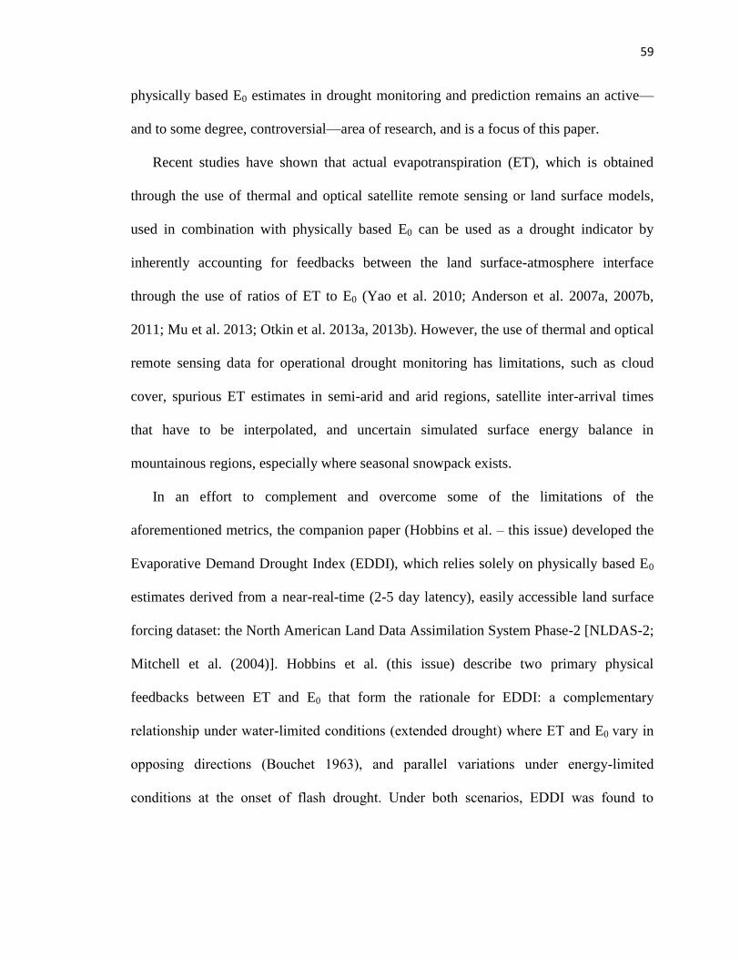
59

physically based E0 estimates in drought monitoring and prediction remains an active—

and to some degree, controversial—area of research, and is a focus of this paper.

Recent studies have shown that actual evapotranspiration (ET), which is obtained

through the use of thermal and optical satellite remote sensing or land surface models,

used in combination with physically based E0 can be used as a drought indicator by

inherently accounting for feedbacks between the land surface-atmosphere interface

through the use of ratios of ET to E0 (Yao et al. 2010; Anderson et al. 2007a, 2007b,

2011; Mu et al. 2013; Otkin et al. 2013a, 2013b). However, the use of thermal and optical

remote sensing data for operational drought monitoring has limitations, such as cloud

cover, spurious ET estimates in semi-arid and arid regions, satellite inter-arrival times

that have to be interpolated, and uncertain simulated surface energy balance in

mountainous regions, especially where seasonal snowpack exists.

In an effort to complement and overcome some of the limitations of the

aforementioned metrics, the companion paper (Hobbins et al. – this issue) developed the

Evaporative Demand Drought Index (EDDI), which relies solely on physically based E0

estimates derived from a near-real-time (2-5 day latency), easily accessible land surface

forcing dataset: the North American Land Data Assimilation System Phase-2 [NLDAS-2;

Mitchell et al. (2004)]. Hobbins et al. (this issue) describe two primary physical

feedbacks between ET and E0 that form the rationale for EDDI: a complementary

relationship under water-limited conditions (extended drought) where ET and E0 vary in

opposing directions (Bouchet 1963), and parallel variations under energy-limited

conditions at the onset of flash drought. Under both scenarios, EDDI was found to

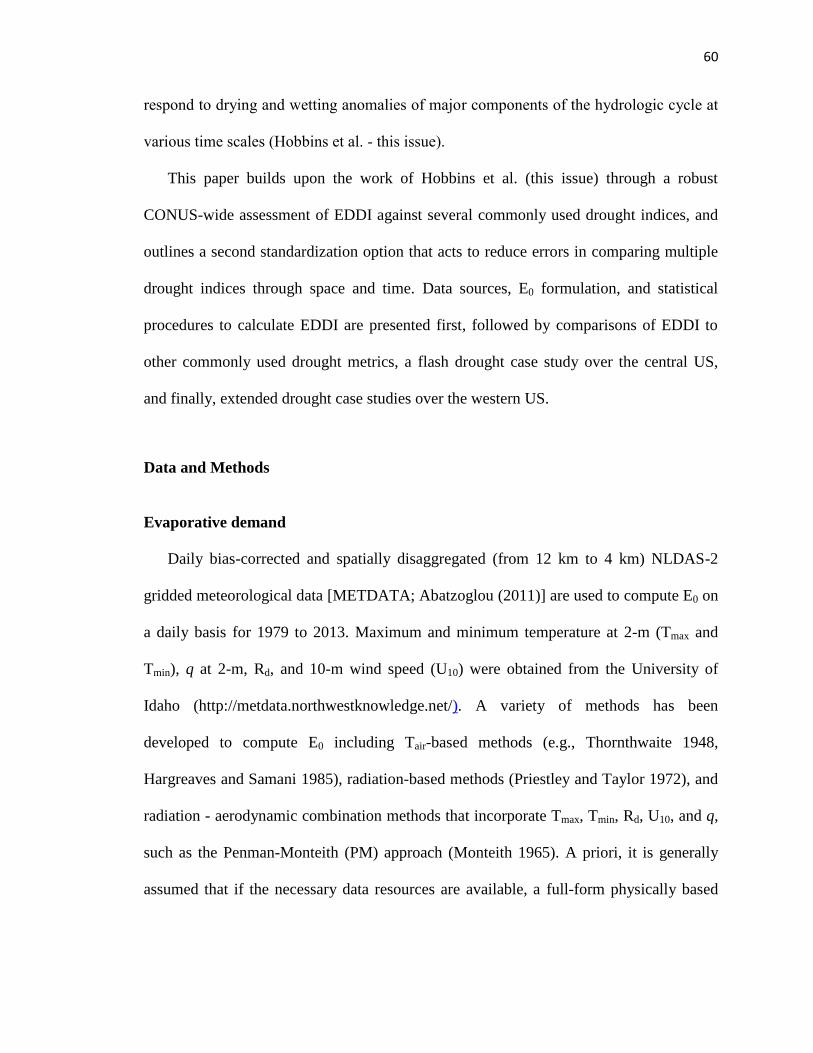
60

respond to drying and wetting anomalies of major components of the hydrologic cycle at

various time scales (Hobbins et al. - this issue).

This paper builds upon the work of Hobbins et al. (this issue) through a robust

CONUS-wide assessment of EDDI against several commonly used drought indices, and

outlines a second standardization option that acts to reduce errors in comparing multiple

drought indices through space and time. Data sources, E0 formulation, and statistical

procedures to calculate EDDI are presented first, followed by comparisons of EDDI to

other commonly used drought metrics, a flash drought case study over the central US,

and finally, extended drought case studies over the western US.

Data and Methods

Evaporative demand

Daily bias-corrected and spatially disaggregated (from 12 km to 4 km) NLDAS-2

gridded meteorological data [METDATA; Abatzoglou (2011)] are used to compute E0 on

a daily basis for 1979 to 2013. Maximum and minimum temperature at 2-m (Tmax and

Tmin), q at 2-m, Rd, and 10-m wind speed (U10) were obtained from the University of

Idaho (http://metdata.northwestknowledge.net/). A variety of methods has been

developed to compute E0 including Tair-based methods (e.g., Thornthwaite 1948,

Hargreaves and Samani 1985), radiation-based methods (Priestley and Taylor 1972), and

radiation - aerodynamic combination methods that incorporate Tmax, Tmin, Rd, U10, and q,

such as the Penman-Monteith (PM) approach (Monteith 1965). A priori, it is generally

assumed that if the necessary data resources are available, a full-form physically based

61

method, such as PM, should be used over methods based only on Tair or radiation.

Hobbins et al. (2012) and Hobbins (2015) demonstrated that the primary drivers of E0

variability differ across the US, and with aggregation period (e.g., monthly vs. annual)

and season. For example, during summer months U10 is the primary driver of E0

variability over much of the Great Basin, while Rd is the primary driver of variability

over much of the southeast US. In this study, we use reference ET (ET0) from the PM-

based American Society of Civil Engineers Standardized Reference ET equation (ASCE-

EWRI, 2005) for E0.

Evaporative Demand Drought Index

A probability-based standardized climate variable can be obtained using parametric or

non-parametric methods. Parametric methods use a single probability distribution to fit a

time series (e.g., Gamma distribution for SPI), where probabilities are transformed to

standardized values through an inverse normal approximation. However, a single

probability distribution may not always be appropriate at large spatial scales, and several

studies have documented these limitations with SPI (Guttman 1999; Quiring 2009) and

Standardized Streamflow Index (Vicente-Serrano et al. 2012). The Evaporative Demand

Drought Index (EDDI) presented in Hobbins et al. (this issue) is calculated from a simple

Z-score based on the mean and standard deviation of a given accumulated ET0 time

series. Here, we deviate from Hobbins et al. (this issue) by using a probability-based

approach for EDDI to allow for more consistent comparisons between EDDI against

other standardized indices.

To overcome the limitations of a parametric approach, ET0 probabilities (P(x)) are

obtained through the empirical Tukey plotting position (Wilkes 2011):

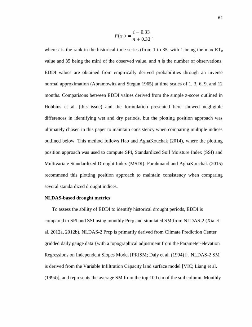
62

𝑃(𝑥𝑖) =𝑖 − 0.33

𝑛 + 0.33 ,

where i is the rank in the historical time series (from 1 to 35, with 1 being the max ET0

value and 35 being the min) of the observed value, and n is the number of observations.

EDDI values are obtained from empirically derived probabilities through an inverse

normal approximation (Abramowitz and Stegun 1965) at time scales of 1, 3, 6, 9, and 12

months. Comparisons between EDDI values derived from the simple z-score outlined in

Hobbins et al. (this issue) and the formulation presented here showed negligible

differences in identifying wet and dry periods, but the plotting position approach was

ultimately chosen in this paper to maintain consistency when comparing multiple indices

outlined below. This method follows Hao and AghaKouchak (2014), where the plotting

position approach was used to compute SPI, Standardized Soil Moisture Index (SSI) and

Multivariate Standardized Drought Index (MSDI). Farahmand and AghaKouchak (2015)

recommend this plotting position approach to maintain consistency when comparing

several standardized drought indices.

NLDAS-based drought metrics

To assess the ability of EDDI to identify historical drought periods, EDDI is

compared to SPI and SSI using monthly Prcp and simulated SM from NLDAS-2 (Xia et

al. 2012a, 2012b). NLDAS-2 Prcp is primarily derived from Climate Prediction Center

gridded daily gauge data {with a topographical adjustment from the Parameter-elevation

Regressions on Independent Slopes Model [PRISM; Daly et al. (1994)]}. NLDAS-2 SM

is derived from the Variable Infiltration Capacity land surface model [VIC; Liang et al.

(1994)], and represents the average SM from the top 100 cm of the soil column. Monthly

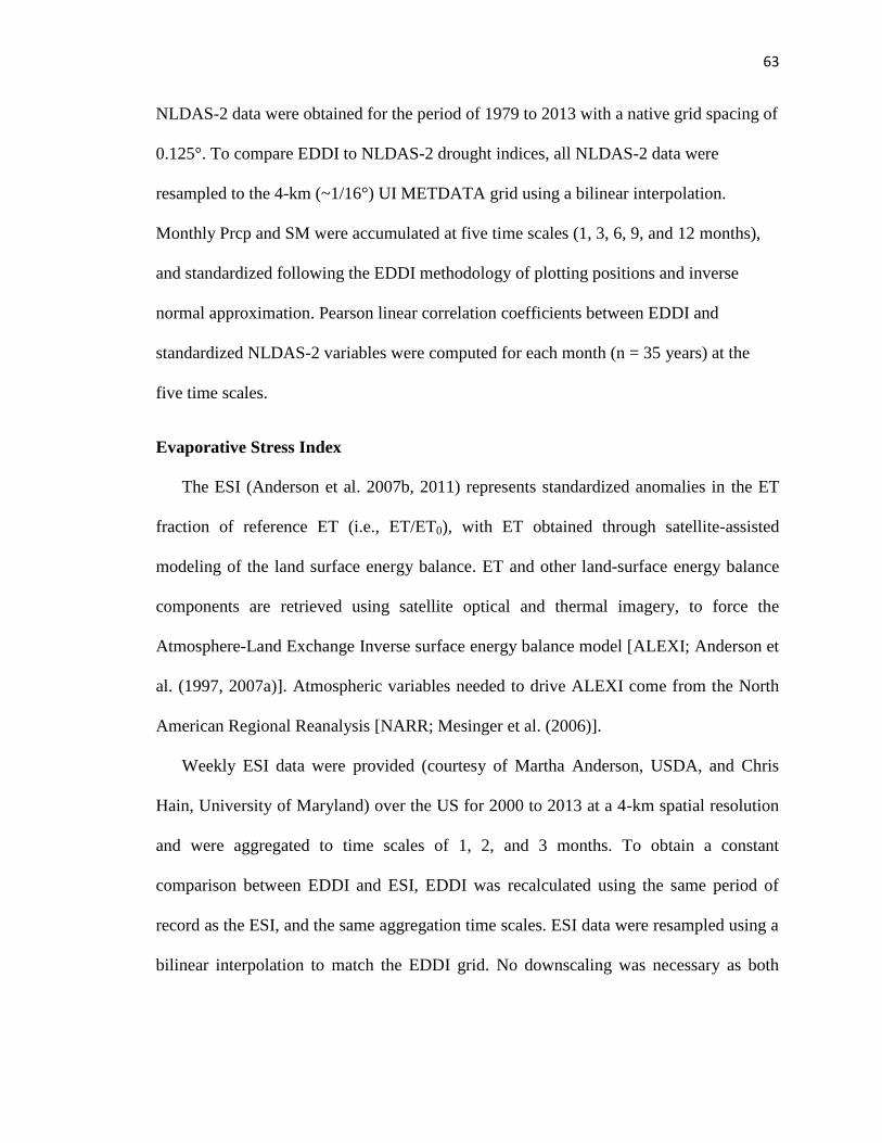
63

NLDAS-2 data were obtained for the period of 1979 to 2013 with a native grid spacing of

0.125°. To compare EDDI to NLDAS-2 drought indices, all NLDAS-2 data were

resampled to the 4-km (~1/16°) UI METDATA grid using a bilinear interpolation.

Monthly Prcp and SM were accumulated at five time scales (1, 3, 6, 9, and 12 months),

and standardized following the EDDI methodology of plotting positions and inverse

normal approximation. Pearson linear correlation coefficients between EDDI and

standardized NLDAS-2 variables were computed for each month (n = 35 years) at the

five time scales.

Evaporative Stress Index

The ESI (Anderson et al. 2007b, 2011) represents standardized anomalies in the ET

fraction of reference ET (i.e., ET/ET0), with ET obtained through satellite-assisted

modeling of the land surface energy balance. ET and other land-surface energy balance

components are retrieved using satellite optical and thermal imagery, to force the

Atmosphere-Land Exchange Inverse surface energy balance model [ALEXI; Anderson et

al. (1997, 2007a)]. Atmospheric variables needed to drive ALEXI come from the North

American Regional Reanalysis [NARR; Mesinger et al. (2006)].

Weekly ESI data were provided (courtesy of Martha Anderson, USDA, and Chris

Hain, University of Maryland) over the US for 2000 to 2013 at a 4-km spatial resolution

and were aggregated to time scales of 1, 2, and 3 months. To obtain a constant

comparison between EDDI and ESI, EDDI was recalculated using the same period of

record as the ESI, and the same aggregation time scales. ESI data were resampled using a

bilinear interpolation to match the EDDI grid. No downscaling was necessary as both

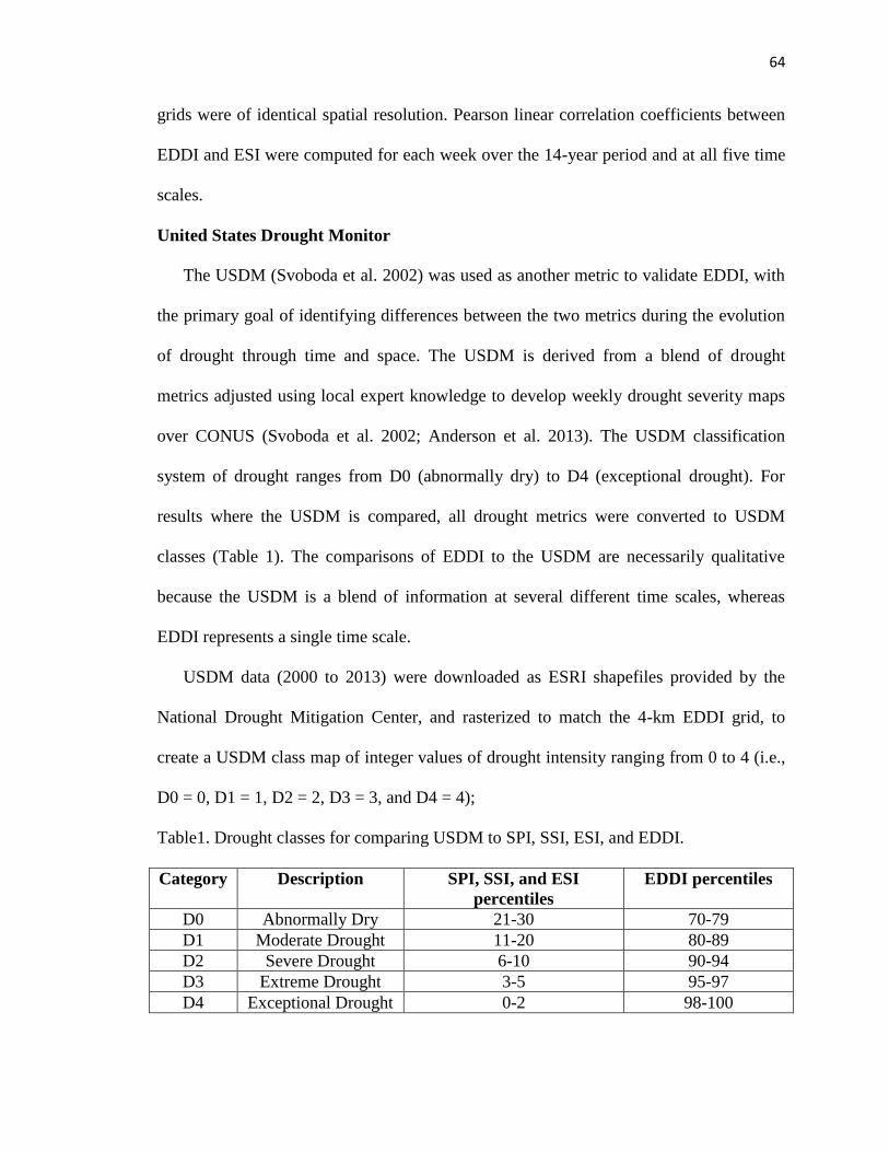
64

grids were of identical spatial resolution. Pearson linear correlation coefficients between

EDDI and ESI were computed for each week over the 14-year period and at all five time

scales.

United States Drought Monitor

The USDM (Svoboda et al. 2002) was used as another metric to validate EDDI, with

the primary goal of identifying differences between the two metrics during the evolution

of drought through time and space. The USDM is derived from a blend of drought

metrics adjusted using local expert knowledge to develop weekly drought severity maps

over CONUS (Svoboda et al. 2002; Anderson et al. 2013). The USDM classification

system of drought ranges from D0 (abnormally dry) to D4 (exceptional drought). For

results where the USDM is compared, all drought metrics were converted to USDM

classes (Table 1). The comparisons of EDDI to the USDM are necessarily qualitative

because the USDM is a blend of information at several different time scales, whereas

EDDI represents a single time scale.

USDM data (2000 to 2013) were downloaded as ESRI shapefiles provided by the

National Drought Mitigation Center, and rasterized to match the 4-km EDDI grid, to

create a USDM class map of integer values of drought intensity ranging from 0 to 4 (i.e.,

D0 = 0, D1 = 1, D2 = 2, D3 = 3, and D4 = 4);

Table1. Drought classes for comparing USDM to SPI, SSI, ESI, and EDDI.

Category Description SPI, SSI, and ESI

percentiles

EDDI percentiles

D0 Abnormally Dry 21-30 70-79

D1 Moderate Drought 11-20 80-89

D2 Severe Drought 6-10 90-94

D3 Extreme Drought 3-5 95-97

D4 Exceptional Drought 0-2 98-100

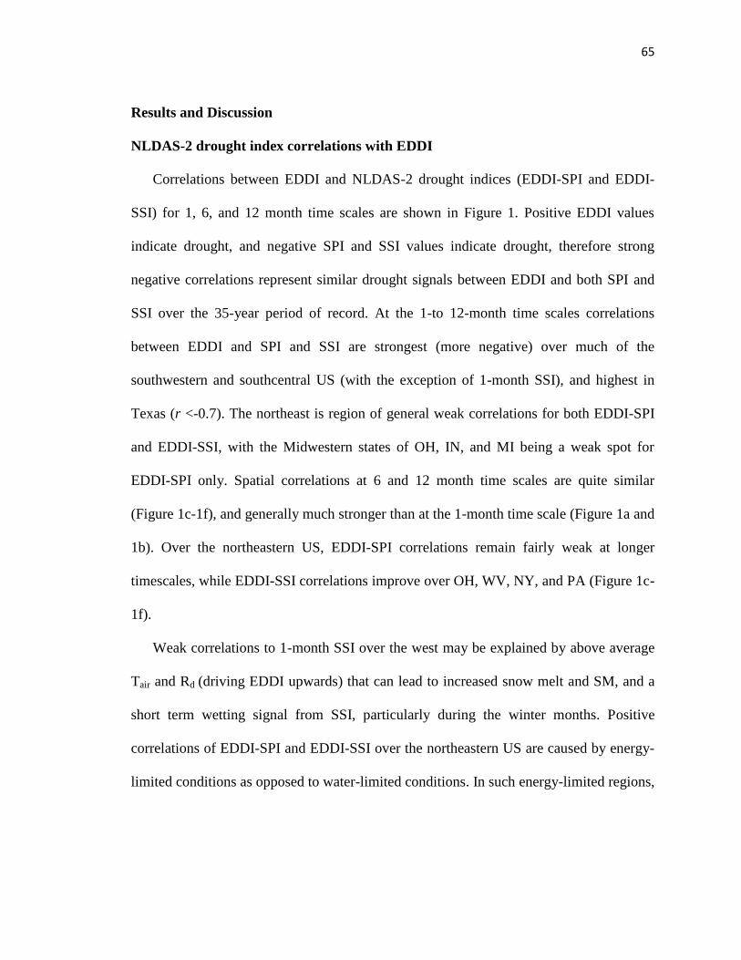
65

Results and Discussion

NLDAS-2 drought index correlations with EDDI

Correlations between EDDI and NLDAS-2 drought indices (EDDI-SPI and EDDI-

SSI) for 1, 6, and 12 month time scales are shown in Figure 1. Positive EDDI values

indicate drought, and negative SPI and SSI values indicate drought, therefore strong

negative correlations represent similar drought signals between EDDI and both SPI and

SSI over the 35-year period of record. At the 1-to 12-month time scales correlations

between EDDI and SPI and SSI are strongest (more negative) over much of the

southwestern and southcentral US (with the exception of 1-month SSI), and highest in

Texas (r <-0.7). The northeast is region of general weak correlations for both EDDI-SPI

and EDDI-SSI, with the Midwestern states of OH, IN, and MI being a weak spot for

EDDI-SPI only. Spatial correlations at 6 and 12 month time scales are quite similar

(Figure 1c-1f), and generally much stronger than at the 1-month time scale (Figure 1a and

1b). Over the northeastern US, EDDI-SPI correlations remain fairly weak at longer

timescales, while EDDI-SSI correlations improve over OH, WV, NY, and PA (Figure 1c-

1f).

Weak correlations to 1-month SSI over the west may be explained by above average

Tair and Rd (driving EDDI upwards) that can lead to increased snow melt and SM, and a

short term wetting signal from SSI, particularly during the winter months. Positive

correlations of EDDI-SPI and EDDI-SSI over the northeastern US are caused by energy-

limited conditions as opposed to water-limited conditions. In such energy-limited regions,

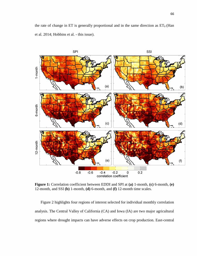
66

the rate of change in ET is generally proportional and in the same direction as ET0 (Han

et al. 2014; Hobbins et al. - this issue).

Figure 1: Correlation coefficient between EDDI and SPI at (a) 1-month, (c) 6-month, (e)

12-month, and SSI (b) 1-month, (d) 6-month, and (f) 12-month time scales.

Figure 2 highlights four regions of interest selected for individual monthly correlation

analysis. The Central Valley of California (CA) and Iowa (IA) are two major agricultural

regions where drought impacts can have adverse effects on crop production. East-central

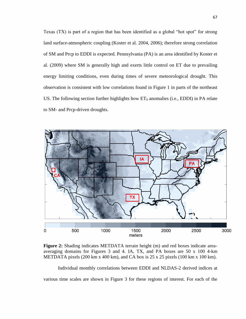
67

Texas (TX) is part of a region that has been identified as a global “hot spot” for strong

land surface-atmospheric coupling (Koster et al. 2004, 2006); therefore strong correlation

of SM and Prcp to EDDI is expected. Pennsylvania (PA) is an area identified by Koster et

al. (2009) where SM is generally high and exerts little control on ET due to prevailing

energy limiting conditions, even during times of severe meteorological drought. This

observation is consistent with low correlations found in Figure 1 in parts of the northeast

US. The following section further highlights how ET0 anomalies (i.e., EDDI) in PA relate

to SM- and Prcp-driven droughts.

Figure 2: Shading indicates METDATA terrain height (m) and red boxes indicate area-

averaging domains for Figures 3 and 4. IA, TX, and PA boxes are 50 x 100 4-km

METDATA pixels (200 km x 400 km), and CA box is 25 x 25 pixels (100 km x 100 km).

Individual monthly correlations between EDDI and NLDAS-2 derived indices at

various time scales are shown in Figure 3 for these regions of interest. For each of the

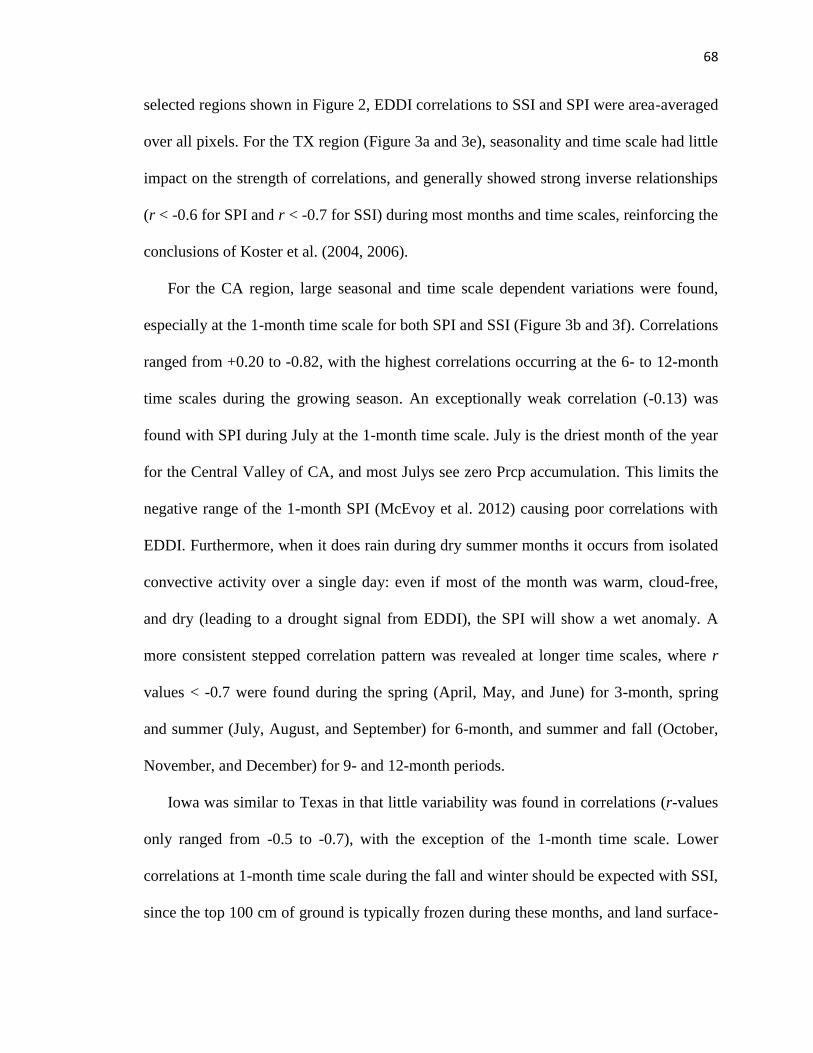
68

selected regions shown in Figure 2, EDDI correlations to SSI and SPI were area-averaged

over all pixels. For the TX region (Figure 3a and 3e), seasonality and time scale had little

impact on the strength of correlations, and generally showed strong inverse relationships

(r < -0.6 for SPI and r < -0.7 for SSI) during most months and time scales, reinforcing the

conclusions of Koster et al. (2004, 2006).

For the CA region, large seasonal and time scale dependent variations were found,

especially at the 1-month time scale for both SPI and SSI (Figure 3b and 3f). Correlations

ranged from +0.20 to -0.82, with the highest correlations occurring at the 6- to 12-month

time scales during the growing season. An exceptionally weak correlation (-0.13) was

found with SPI during July at the 1-month time scale. July is the driest month of the year

for the Central Valley of CA, and most Julys see zero Prcp accumulation. This limits the

negative range of the 1-month SPI (McEvoy et al. 2012) causing poor correlations with

EDDI. Furthermore, when it does rain during dry summer months it occurs from isolated

convective activity over a single day: even if most of the month was warm, cloud-free,

and dry (leading to a drought signal from EDDI), the SPI will show a wet anomaly. A

more consistent stepped correlation pattern was revealed at longer time scales, where r

values < -0.7 were found during the spring (April, May, and June) for 3-month, spring

and summer (July, August, and September) for 6-month, and summer and fall (October,

November, and December) for 9- and 12-month periods.

Iowa was similar to Texas in that little variability was found in correlations (r-values

only ranged from -0.5 to -0.7), with the exception of the 1-month time scale. Lower

correlations at 1-month time scale during the fall and winter should be expected with SSI,

since the top 100 cm of ground is typically frozen during these months, and land surface-

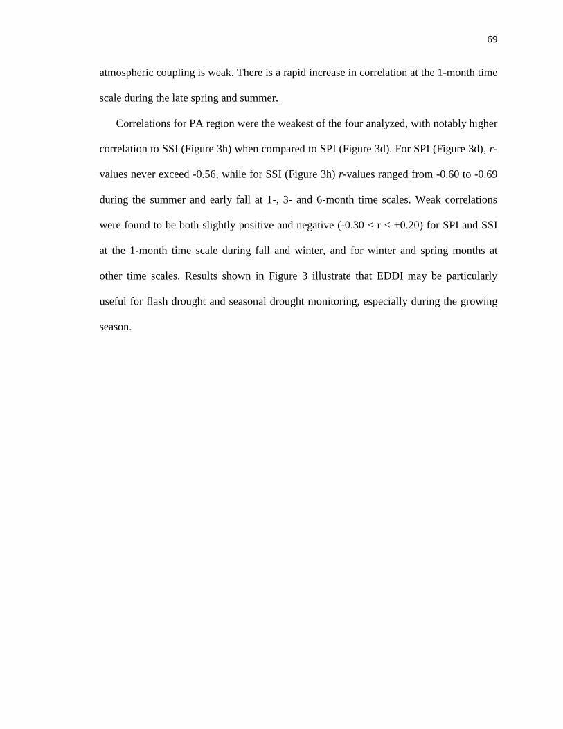
69

atmospheric coupling is weak. There is a rapid increase in correlation at the 1-month time

scale during the late spring and summer.

Correlations for PA region were the weakest of the four analyzed, with notably higher

correlation to SSI (Figure 3h) when compared to SPI (Figure 3d). For SPI (Figure 3d), r-

values never exceed -0.56, while for SSI (Figure 3h) r-values ranged from -0.60 to -0.69

during the summer and early fall at 1-, 3- and 6-month time scales. Weak correlations

were found to be both slightly positive and negative (-0.30 < r < +0.20) for SPI and SSI

at the 1-month time scale during fall and winter, and for winter and spring months at

other time scales. Results shown in Figure 3 illustrate that EDDI may be particularly

useful for flash drought and seasonal drought monitoring, especially during the growing

season.

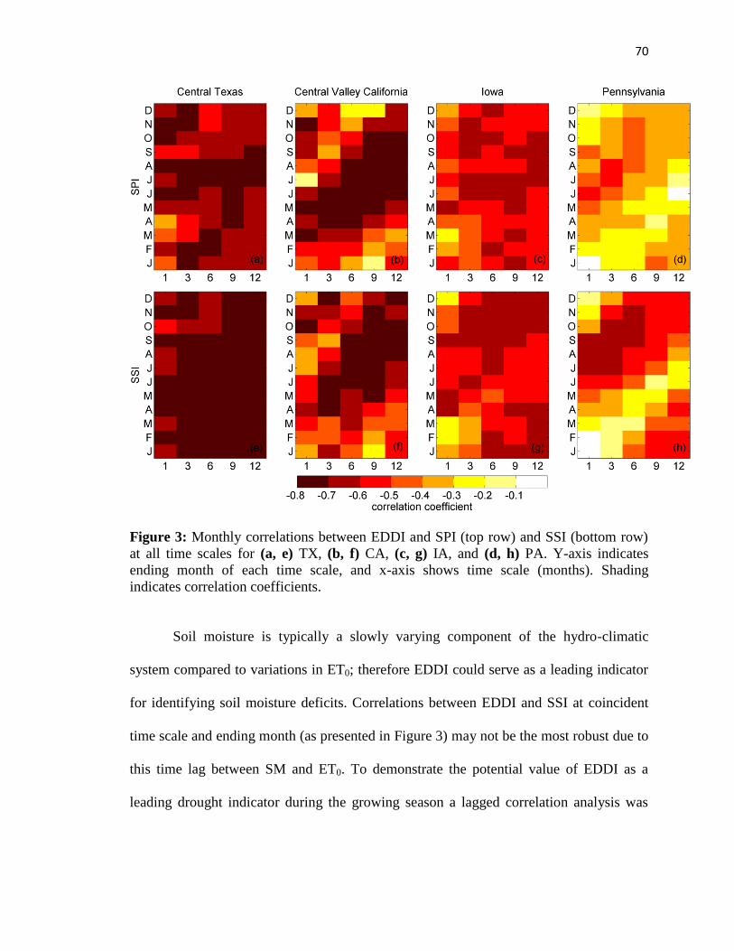
70

Figure 3: Monthly correlations between EDDI and SPI (top row) and SSI (bottom row)

at all time scales for (a, e) TX, (b, f) CA, (c, g) IA, and (d, h) PA. Y-axis indicates

ending month of each time scale, and x-axis shows time scale (months). Shading

indicates correlation coefficients.

Soil moisture is typically a slowly varying component of the hydro-climatic

system compared to variations in ET0; therefore EDDI could serve as a leading indicator

for identifying soil moisture deficits. Correlations between EDDI and SSI at coincident

time scale and ending month (as presented in Figure 3) may not be the most robust due to

this time lag between SM and ET0. To demonstrate the potential value of EDDI as a

leading drought indicator during the growing season a lagged correlation analysis was

71

performed between 3-month SSI ending in August and EDDI at every time scale and

ending month.

Figure 4 shows that in all four regions EDDI leads SSI, where 3-month SSI ending in

August (blue dots in Figure 4 show fixed time scale and ending month for SSI) is better

correlated to 3-month EDDI ending in June (CA; Figure 4a) or July (TX, IA, and PA;

Figure 4b, 4c, and 4d respectively). An interesting feature of Figure 4 is shown for IA,

where 12-month EDDI ending in August was found to have highest correlation to 3-

month SSI ending in August, highlighting the extremely low summer SM moisture

variability in this region. This is further reinforced later in Figure 6, where monthly SSI

variability was found to be low relative to EDDI and SPI during the 2012 drought. These

results highlight that EDDI is a leading indicator when compared to SSI, and therefore

could be used to complement and perhaps improve the USDM since SM percentiles are

primary inputs for USDM objective blends.

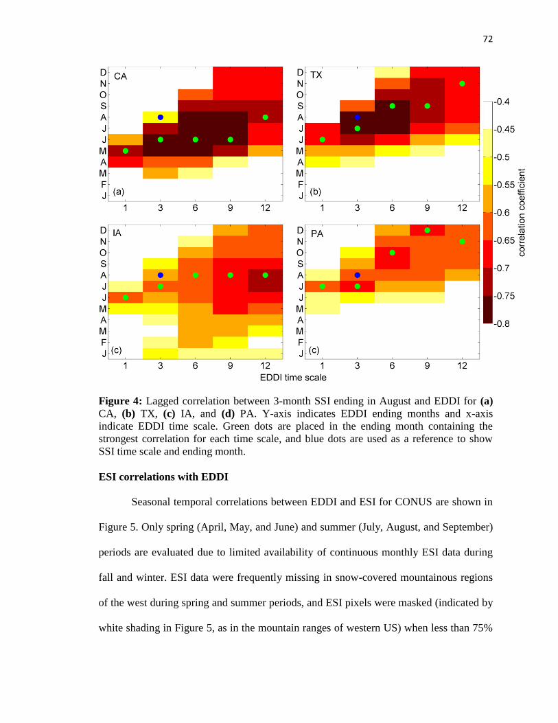
72

Figure 4: Lagged correlation between 3-month SSI ending in August and EDDI for (a)

CA, (b) TX, (c) IA, and (d) PA. Y-axis indicates EDDI ending months and x-axis

indicate EDDI time scale. Green dots are placed in the ending month containing the

strongest correlation for each time scale, and blue dots are used as a reference to show

SSI time scale and ending month.

ESI correlations with EDDI

Seasonal temporal correlations between EDDI and ESI for CONUS are shown in

Figure 5. Only spring (April, May, and June) and summer (July, August, and September)

periods are evaluated due to limited availability of continuous monthly ESI data during

fall and winter. ESI data were frequently missing in snow-covered mountainous regions

of the west during spring and summer periods, and ESI pixels were masked (indicated by

white shading in Figure 5, as in the mountain ranges of western US) when less than 75%

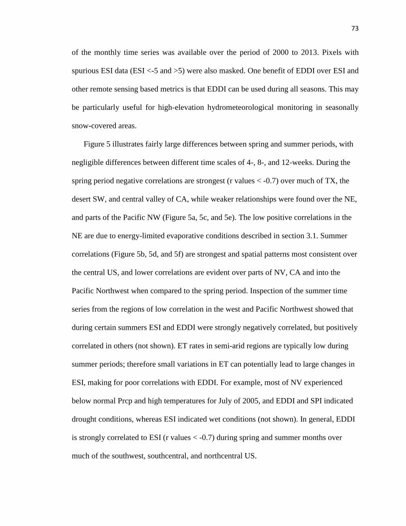
73

of the monthly time series was available over the period of 2000 to 2013. Pixels with

spurious ESI data (ESI <-5 and >5) were also masked. One benefit of EDDI over ESI and

other remote sensing based metrics is that EDDI can be used during all seasons. This may

be particularly useful for high-elevation hydrometeorological monitoring in seasonally

snow-covered areas.

Figure 5 illustrates fairly large differences between spring and summer periods, with

negligible differences between different time scales of 4-, 8-, and 12-weeks. During the

spring period negative correlations are strongest (r values < -0.7) over much of TX, the

desert SW, and central valley of CA, while weaker relationships were found over the NE,

and parts of the Pacific NW (Figure 5a, 5c, and 5e). The low positive correlations in the

NE are due to energy-limited evaporative conditions described in section 3.1. Summer

correlations (Figure 5b, 5d, and 5f) are strongest and spatial patterns most consistent over

the central US, and lower correlations are evident over parts of NV, CA and into the

Pacific Northwest when compared to the spring period. Inspection of the summer time

series from the regions of low correlation in the west and Pacific Northwest showed that

during certain summers ESI and EDDI were strongly negatively correlated, but positively

correlated in others (not shown). ET rates in semi-arid regions are typically low during

summer periods; therefore small variations in ET can potentially lead to large changes in

ESI, making for poor correlations with EDDI. For example, most of NV experienced

below normal Prcp and high temperatures for July of 2005, and EDDI and SPI indicated

drought conditions, whereas ESI indicated wet conditions (not shown). In general, EDDI

is strongly correlated to ESI (r values < -0.7) during spring and summer months over

much of the southwest, southcentral, and northcentral US.

74

Figure 5: Seasonal correlation coefficient (left column spring and right column summer)

between ESI and EDDI at (a, b) 4-week, (c, d) 8-week, and (e, f) 12-week time scales.

Areas shaded in white indicate an insufficient amount of ESI data.

Flash drought over the central US

Flash drought can develop even during periods of excess Prcp, and evaporative

drivers can potentially uniquely identify the onset and evolution of flash drought. For

example, in some situations (i.e., the 2011 central CONUS case), a T-based E0 would fail

to identify rapid drying due to below normal Tair coincident with high U2 and low q. The

following highlights the Midwest droughts of 2011 and 2012 as a case study to

75

demonstrate how EDDI can serve as an effective early warning of flash droughts, as well

as extended droughts.

Area-averaged time series of 1-month EDDI are compared to 1-month SPI and SSI

during 2011 and 2012 in Figure 6a for the IA domain. Figure 6b illustrates the sensitivity

of EDDI to individual ET0 forcings averaged over the IA domain. Note that in Figures 6a

and 6b the vertical axis of EDDI is reversed to better visualize drought onset and duration

when compared to SPI and SSI. Figure 6a illustrates that in April, 2011, all indices are

near neutral (i.e., close to zero), and over the next two months EDDI changes to a

moderate drought class (<-0.78 or USDM D1 class), while both SPI and SSI increase to

slightly wet conditions. SPI and SSI values do not decrease towards moderate drought

conditions until July of 2011. SPI falls below moderate drought in September, and SSI

follows one month later in October. Both EDDI and SSI maintain extended drought

conditions throughout all of 2012, with the exception of February when EDDI is slightly

above moderate drought (-0.78), but still below zero. During this extended drought of

2012, SPI is highly variable and indicates wet conditions for many months.

To highlight the ET0 drivers that caused EDDI to signal first a flash drought and then

an extended drought, a simple sensitivity analysis of EDDI was performed (Figure 6b and

6c). For this analysis, ET0 was calculated while constraining the variable of interest to

daily climatology values in order to isolate the impact of each forcing on the EDDI

drought signal. Results are presented as estimates of EDDI with a notation of the variable

constrained to its daily climatology (i.e., EDDI-T, EDDI-q, EDDI-Rd, and EDDI-U2). For

example, EDDI-T was calculated using the daily climatology of Tmax and Tmin, and with

METDATA-observed forcings values of all other variables. During the period of 20 May

76

to 25 May, EDDI-q and EDDI-U2 had the greatest separation from standard EDDI values

in the negative direction (note y-axis is reversed), which indicates that the drying power

of the air term in the ET0 equation, (U2 multiplied by vapor pressure deficit), initiated the

flash drought signal—approximately 20 May through 5 June—in EDDI via increased U2

and below normal q (Figure 6c). In this case, using daily climatology q and U2 values

mitigated the drought signal relative to the standard EDDI. By June, 2011, EDDI

decreased below the moderate drought threshold (-0.78), with the primary difference

from May being that U2 and Tair were then acting in combination to exacerbate the

drought signal—as opposed to Tair moderating it in May. Despite below-normal Tair

conditions in September, 2011, the standard EDDI drought signal was maintained due to

extremely low q values evidenced by a large difference between EDDI and EDDI-q

(absolute difference of 1.17). From November, 2011, through the following May, Tair

dominated the EDDI signal, as seen by the large differences between EDDI and EDDI-T.

This increase in Tair and ET0 likely contributed to the persistent SSI drought signal

throughout 2012, despite above-normal Prcp for February, April, October, and December

(Figure 6a).

Results illustrated in Figure 6 and in the companion paper of Hobbins et al.

(2015) highlight two major focal points of this research: (1) EDDI is a leading indicator

of flash and extended drought conditions, and (2) a physically based E0 is required to

capture this signal. This reinforces the work of Hobbins et al. (2012) and Hobbins (2015)

who concluded that Tair is not always the dominant driver of ET0, and T-based

parameterizations could lead to false drying (or wetting) signals when used for drought

monitoring applications. Our findings illustrated in Figure 6 also contradict the notion

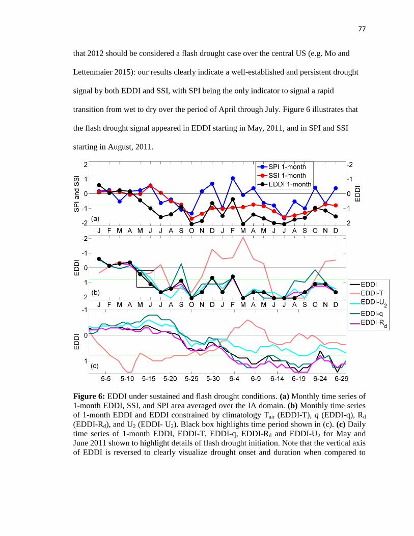
77

that 2012 should be considered a flash drought case over the central US (e.g. Mo and

Lettenmaier 2015): our results clearly indicate a well-established and persistent drought

signal by both EDDI and SSI, with SPI being the only indicator to signal a rapid

transition from wet to dry over the period of April through July. Figure 6 illustrates that

the flash drought signal appeared in EDDI starting in May, 2011, and in SPI and SSI

starting in August, 2011.

Figure 6: EDDI under sustained and flash drought conditions. (a) Monthly time series of

1-month EDDI, SSI, and SPI area averaged over the IA domain. (b) Monthly time series

of 1-month EDDI and EDDI constrained by climatology Tair (EDDI-T), q (EDDI-q), Rd

(EDDI-Rd), and U2 (EDDI- U2). Black box highlights time period shown in (c). (c) Daily

time series of 1-month EDDI, EDDI-T, EDDI-q, EDDI-Rd and EDDI-U2 for May and

June 2011 shown to highlight details of flash drought initiation. Note that the vertical axis

of EDDI is reversed to clearly visualize drought onset and duration when compared to

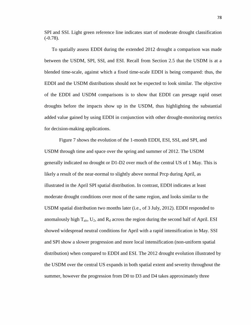
78

SPI and SSI. Light green reference line indicates start of moderate drought classification

(-0.78).

To spatially assess EDDI during the extended 2012 drought a comparison was made

between the USDM, SPI, SSI, and ESI. Recall from Section 2.5 that the USDM is at a

blended time-scale, against which a fixed time-scale EDDI is being compared: thus, the

EDDI and the USDM distributions should not be expected to look similar. The objective

of the EDDI and USDM comparisons is to show that EDDI can presage rapid onset

droughts before the impacts show up in the USDM, thus highlighting the substantial

added value gained by using EDDI in conjunction with other drought-monitoring metrics

for decision-making applications.

Figure 7 shows the evolution of the 1-month EDDI, ESI, SSI, and SPI, and

USDM through time and space over the spring and summer of 2012. The USDM

generally indicated no drought or D1-D2 over much of the central US of 1 May. This is

likely a result of the near-normal to slightly above normal Prcp during April, as

illustrated in the April SPI spatial distribution. In contrast, EDDI indicates at least

moderate drought conditions over most of the same region, and looks similar to the

USDM spatial distribution two months later (i.e., of 3 July, 2012). EDDI responded to

anomalously high Tair, U2, and Rd across the region during the second half of April. ESI

showed widespread neutral conditions for April with a rapid intensification in May. SSI

and SPI show a slower progression and more local intensification (non-uniform spatial

distribution) when compared to EDDI and ESI. The 2012 drought evolution illustrated by

the USDM over the central US expands in both spatial extent and severity throughout the

summer, however the progression from D0 to D3 and D4 takes approximately three

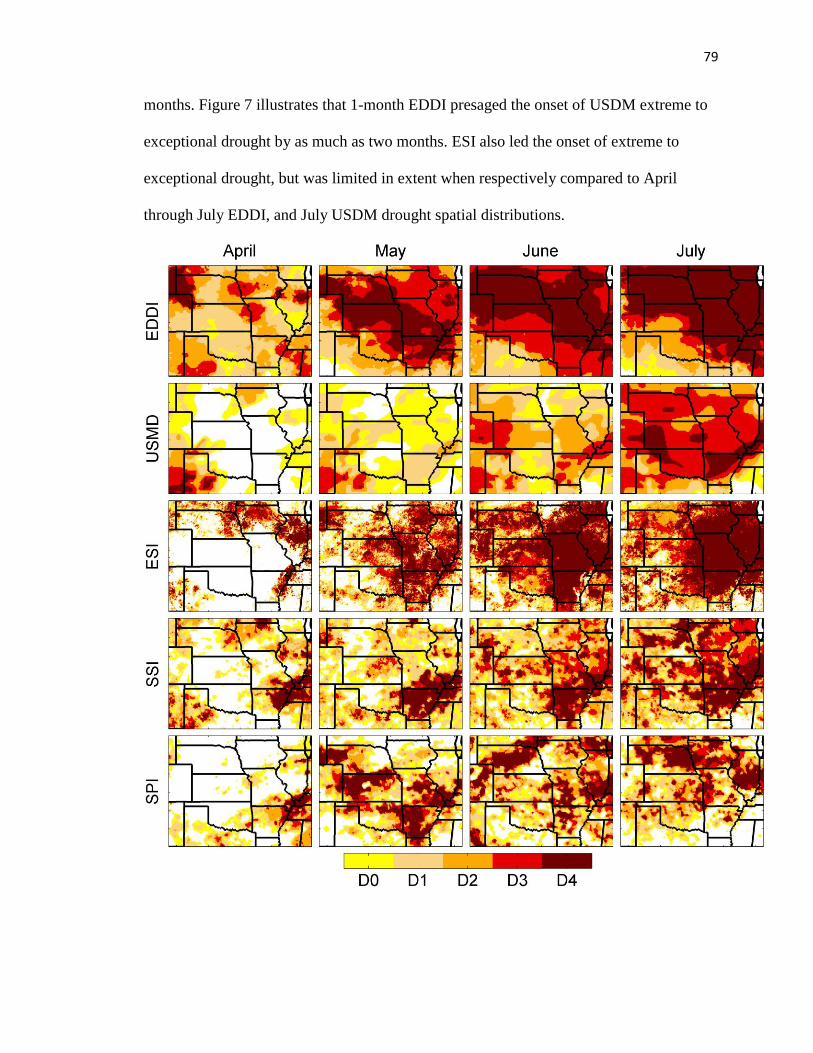
79

months. Figure 7 illustrates that 1-month EDDI presaged the onset of USDM extreme to

exceptional drought by as much as two months. ESI also led the onset of extreme to

exceptional drought, but was limited in extent when respectively compared to April

through July EDDI, and July USDM drought spatial distributions.

80

Figure 7: Evolution of the 1-month EDDI (top row), USDM (second row), 1-month ESI

(third row), 1-month SSI (fourth row), and 1-month SPI (fifth row) through spring and

summer of 2012. USDM data are from 1 May, 2012 (April column), 5 June, 2012 (May

column), 3 July, 2012 (June column), and 31 July, 2012 (July column). EDDI, ESI, SSI,

and SPI are at 1-month time scales at the end of each month: April, May, June, and July.

All drought metrics have been converted to USDM categories according to Table 1.

Extended drought in arid to semi-arid regions

In this section we examine whether EDDI can be used to characterize historical

extended droughts over the western US. Droughts in arid to semi-arid regions of the US

are generally slower to develop than in the central US, primarily due to the manner in

which water resources are both naturally and anthropogenically stored. Natural water

storage occurs as winter snowpack at high elevations that typically reach maximum depth

in March or April. During spring and summer snowmelt, runoff is stored in reservoirs.

Hydrologic and agricultural drought severity in the west are strongly linked to reservoir

storage and streamflow (McEvoy et al. 2012, Abatzoglou et al. 2014).

Two extended drought case studies using the USDM, EDDI, SPI, and SSI are shown

in Figure 8. The first case focuses on the drought of the 2007 water year (October 2006

through September 2007) (Figure 8, left column). The USDM from 02 October, 2007,

indicates 78% (percent area) of the western US in at least a D0 drought class. Figure 8c

illustrates the 12-month EDDI ending in September, 2007, and has the strongest spatial

coherence and severity when compared to the USDM, while SSI and SPI (Figure 8e and

8g, respectively) underrepresent the spatial extent shown by USDM and EDDI,

particularly over NV, ID, and western MT. The second case focuses on the extreme

southwestern drought of 2002 (Figure 8, right column), with the USDM mapped at 25

June, 2002, and the 6-month EDDI, SPI, and SPI mapped for January through June, 2002.

81

All metrics show a similar spatial structure of drought extent, although EDDI and SPI

indicate little to no drought in MT. Temperatures were lower than normal over much of

MT, WY, and the northern portion of UT and CO, and slightly above normal for the Four

Corners region (not shown). This indicates that Tair was likely driving EDDI negative in

MT, however Tair, q and U2 must have all played a role in driving EDDI in the positive

direction over UT and CO.

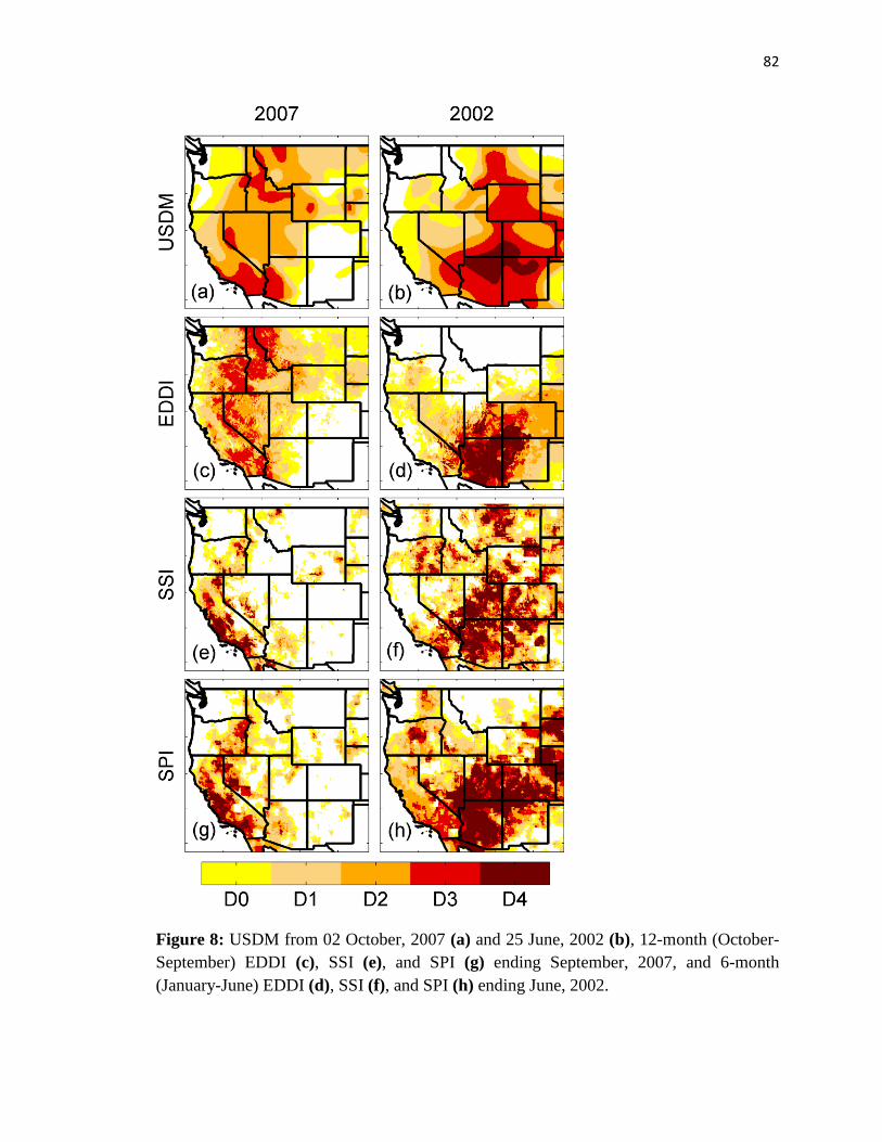
82

Figure 8: USDM from 02 October, 2007 (a) and 25 June, 2002 (b), 12-month (October-

September) EDDI (c), SSI (e), and SPI (g) ending September, 2007, and 6-month

(January-June) EDDI (d), SSI (f), and SPI (h) ending June, 2002.

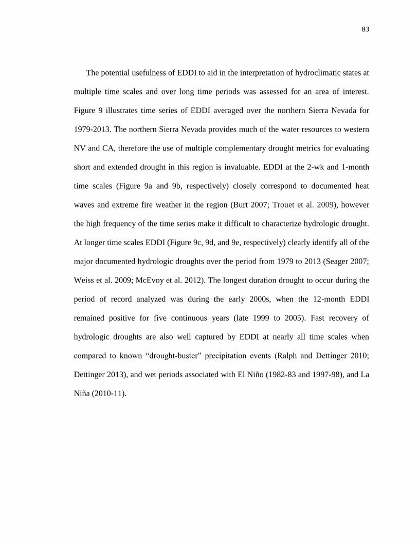
83

The potential usefulness of EDDI to aid in the interpretation of hydroclimatic states at

multiple time scales and over long time periods was assessed for an area of interest.

Figure 9 illustrates time series of EDDI averaged over the northern Sierra Nevada for

1979-2013. The northern Sierra Nevada provides much of the water resources to western

NV and CA, therefore the use of multiple complementary drought metrics for evaluating

short and extended drought in this region is invaluable. EDDI at the 2-wk and 1-month

time scales (Figure 9a and 9b, respectively) closely correspond to documented heat

waves and extreme fire weather in the region (Burt 2007; Trouet et al. 2009), however

the high frequency of the time series make it difficult to characterize hydrologic drought.

At longer time scales EDDI (Figure 9c, 9d, and 9e, respectively) clearly identify all of the

major documented hydrologic droughts over the period from 1979 to 2013 (Seager 2007;

Weiss et al. 2009; McEvoy et al. 2012). The longest duration drought to occur during the

period of record analyzed was during the early 2000s, when the 12-month EDDI

remained positive for five continuous years (late 1999 to 2005). Fast recovery of

hydrologic droughts are also well captured by EDDI at nearly all time scales when

compared to known “drought-buster” precipitation events (Ralph and Dettinger 2010;

Dettinger 2013), and wet periods associated with El Niño (1982-83 and 1997-98), and La

Niña (2010-11).

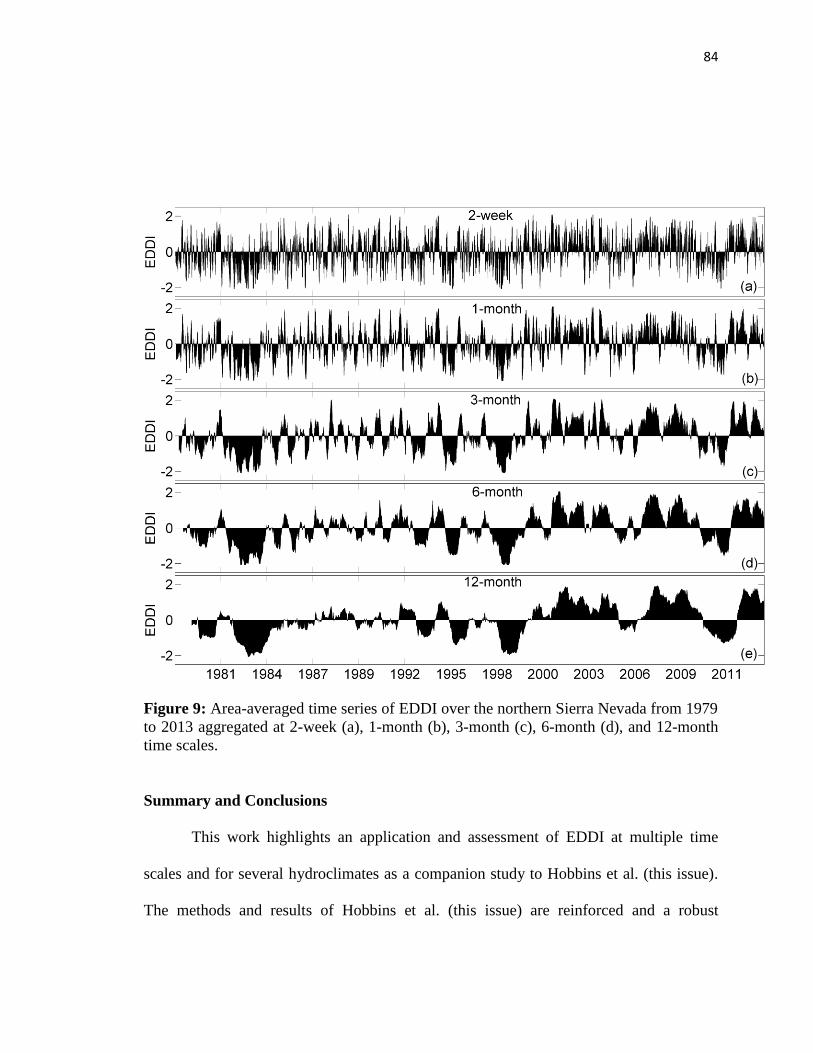
84

Figure 9: Area-averaged time series of EDDI over the northern Sierra Nevada from 1979

to 2013 aggregated at 2-week (a), 1-month (b), 3-month (c), 6-month (d), and 12-month

time scales.


This work highlights an application and assessment of EDDI at multiple time

scales and for several hydroclimates as a companion study to Hobbins et al. (this issue).

The methods and results of Hobbins et al. (this issue) are reinforced and a robust

85

CONUS-wide evaluation is performed, by examining EDDI and individual evaporative

demand components as they relate to the dynamic evolution of flash drought over the

central US, characterization of hydrologic drought over the western US, and comparison

to commonly used drought metrics (USDM, SPI, SSI, and ESI). Results highlight the

advantages and limitations of EDDI as a monitor of drought at multiple time scales, and

provide leading indications of flash and extended hydrologic drought. Correlations of

EDDI to NLDAS-2 forced drought metrics of SSI and SPI indicate that over much of the

CONUS, EDDI spatial distributions are generally similar to SPI and SSI. Over parts of

the western US where weak correlations were found, EDDI often contained drought

information not found in SPI or SSI. For example, Prcp is bounded by zero at short time

scales (1 to 2 months) over many western states, which can lead to a skewed SPI,

whereas EDDI will maintain a consistent distribution during months with no Prcp. At

short time scales, spatial distributions and time series results illustrate that EDDI can be

useful for flash drought identification, and can serve as a leading indicator by as much as

two months in advance of the USDM, SPI, and SSI (i.e. Figures 4, 6, 7; and Figures

shown in Hobbins et al. - this issue).

Comparisons of EDDI to remotely sensed ESI products also show strong correlations,

with the exceptions of the northeast US during spring, and over parts of the western US

during summer. Weak correlations with ESI over the northeastern US are largely due to

energy-limited land-surface energy-balance conditions over the region, where ET and

ET0 are often positively correlated. Weak correlations with ESI over the western US

during summer months are likely due to the low and effectively zero-bounded actual ET

rates that occur in arid environments. Low soil moisture and low ET rates make it

86

difficult to accurately estimate ET with thermal and optical remote sensing. These

uncertainties combined with the high variability of estimated ET relative to average

conditions often led to spurious ESI values and low correlations with EDDI.

Comparisons of EDDI with ESI generally demonstrate that EDDI can be effectively used

in conjunction with ESI and other remote sensing products to provide year-round data,

with no limitations during cloudy days or over snow covered areas.

For drought monitoring in arid and semi-arid regions of western US, EDDI

aggregation to longer time scales (3 to 12 months) is best suited to capture the

complementary relationship found between ET and ET0 (Bouchet 1963; Hobbins et al.

2004), and therefore identify extended hydrologic droughts typical of this region. Results

illustrate that in most cases, when Prcp deficits at the 3- to 12-month time scales were

fairly large, EDDI was strongly positive. However, the complementary relationship was

found to not hold true in regions and time periods where weak land surface-atmospheric

coupling and energy limited conditions exist (Figures 3 and 5).

Despite some noted limitations, EDDI is shown to provide useful information on the

less-understood and documented dynamical processes associated with drought evolution

and persistence. Results highlighted in this work illustrate the benefits of assimilating

physically based E0 estimates and EDDI into operational monitoring products such as the

USDM. The additional information and early warning provided by EDDI could greatly

contribute to a stronger understanding of drought evolution and dynamics, land surface-

atmosphere interactions, and perhaps more importantly, reduce and/or mitigate future

adverse societal effects that have been associated with past droughts. EDDI could also

prove very useful and effective for easy-to-implement operational early warning for

87

agricultural and fire-weather monitoring (Ham et al. 2014) and seasonal forecasting of

drought.

Acknowledgments

This research was supported by the Desert Research Institute (DRI) Maki Endowment

for enhancing water resource monitoring in Southern, Nevada, U.S. Bureau of

Reclamation Climate Analysis Tools WaterSMART program, the National Integrated

Drought Information System (NIDIS) program, and U.S. Geological Survey and DRI

Great Basin Cooperative Ecosystem Study Unit collaborative project on drought

monitoring and fallow field tracking through cloud computing of Landsat, MODIS, and

gridded climate data archives.

References

Abatzoglou, J.T., 2011: Development of gridded surface meteorological data for

ecological

applications and modelling. Int. J. Climatol. 33, 121–131, doi:10.1002/joc.3413.

Abatzoglou, J.T., R. Barbero, J. Wolf, and Z. Holden, 2014: Tracking interannual

streamflow variability with drought indices in the U.S. Pacific Northwest. J.

Hydrometeor. 15, 1900–1912, doi:10.1175/JHM-D-13-0167.1.

Abramowitz, M., and I.A. Stegun, 1965: Handbook of mathematical functions, with

formulas, graphs, and mathematical tables. Dover Publications, 1046 pp.

88

Anderson, M.C., J.M. Norman, G.R. Diak, W.P. Kustas, and J.R. Mecikalski, 1997: A

two-source time-integrated model for estimating surface fluxes using thermal infrared

remote sensing. Remote Sens. Environ., 60, 195–216.

Anderson, M.C., J. M. Norman, J.R. Mecikalski, J.A. Otkin, and W.P. Kustas, 2007: A

climatological study of evapotranspiration and moisture stress across the continental

United States based on thermal remote sensing: 1. Model formulation, J. Geophys.

Res., 112, D10117, doi:10.1029/2006JD007506.

Anderson, M.C., J.M. Norman, J.R. Mecikalski, J.A. Otkin, and W.P. Kustas, 2007: A

climatological study of evapotranspiration and moisture stress across the continental

United States based on thermal remote sensing: 2. Surface moisture climatology, J.

Geophys. Res., 112, D11112, doi:10.1029/2006JD007507.

Anderson, M.C., C. Hain, B. Wardlow, A. Pimstein, J.R. Mecikalski, and W.P. Kustas,

2011: Evaluation of drought indices based on thermal remote sensing of

evapotranspiration over the continental United States. J. Climate, 24(8), 2025–2044,

doi:10.1175/2010JCLI3812.1.

Anderson, M.C., C. Hain, J. Otkin, X. Zhan, K. Mo, M. Svoboda, B. Wardlow, and A.

Pimstein, 2013: An intercomparison of drought indicators based on thermal remote

sensing and NLDAS-2 simulations with U.S. Drought Monitor classifications. J.

Hydrometeor., 14, 1035–1056, doi:10.1175/JHM-D-12-0140.1.

ASCE-EWRI, 2005: The ASCE Standardized Reference Evapotranspiration Equation.

Report 0-7844-0805-X, 59 pp. [Available online at

http://www.kimberly.uidaho.edu/water/asceewri/ascestzdetmain2005.pdf.]

89

Bouchet, R.J., 1963: Évapotranspiration réelle et potentielle, signification climatique.

Proc. International Association Scientific Hydrology Symp., Publ. No. 62, Berkeley,

CA, International Association Scientific Hydrology, 134–142.

Burt, C.C., 2007: Extreme weather: a guide and record book. W.W. Norton and Co., 320

pp.

Cattiaux, J., and P. Yiou, 2013: U.S. heat waves of spring and summer 2012 from the

flow-analogue perspective [in “Explaining Extreme Events of 2012 from a Climate

Perspective”]. Bull. Amer. Meteor. Soc., 94(9), S10–S13.

Dai, A., 2011: Characteristics and trends in various forms of the Palmer Drought Severity

Index during 1900-2008, J. Geophys. Res., 116, D12115,

doi:10.1029/2010JD015541.

Daly, C., R.P. Neilson, and D.L. Phillips, 1994: A statistical-topographic model for

mapping climatological precipitation over mountainous terrain. J. Appl. Meteorol.,

33(2), 140–158.

Dettinger, M.D., 2013. Atmospheric rivers as drought busters on the U.S. West Coast. J.

Hydrometeor., 14(6), 1721–1732, doi: 10.1175/JHM-D-13-02.1.

Farahmand, A., and A. AghaKouchak, 2015: A generalized framework for deriving

nonparametric standardized indicators. Adv. Water Resour., 76, 140–145,

doi:10.1016/j.advwatres.2014.11.012

Guttman, N.B., 1999: Accepting the standardized precipitation index: a calculation

algorithm. J. Amer. Water Resour. Assoc. 35(2), 311–322.

Ham, C., M.T. Hobbins, K.L. Abt, and J.P. Prestemon, 2014: Using the Evaporative

Demand Drought Index and the Palmer Drought Severity Index to forecast the

90

number of large wildland fires on federal lands, Large Wildland Fires Conference,

Missoula, MT, Association for Fire Ecology and the International Association of

Wildland Fire. [Available online at http://largefireconference.org/wp-

content/uploads/2013/06/Oral-Presentation-Abstracts-V4.pdf.]

Han, S., F. Tian, and H. Hu, 2014: Positive or negative correlation between actual and

potential evaporation? Evaluating using a nonlinear complementary relationship

model. Water Resources Research, 50(2), 1322–1336.

Hao, Z., and A. AghaKouchak, 2014: A nonparametric multivariate multi-index drought

monitoring framework, J. Hydrometeor., 15, 89–101, doi:10.1175/JHM-D-12-0160.1.

Hargreaves, G.H., and Z.A. Samani, 1985: Reference crop evapotranspiration from

temperature, Appl. Eng. Agric., 1, 96–99.

Heddinghaus, T.R., and P. Sabol, 1991: A review of the Palmer Drought Severity Index

and where do we go from here? Preprints, Seventh Conf. on Applied Climatology,

Boston, MA, Amer. Meteor. Soc., 242–246. [Available online at

http://www.ncdc.noaa.gov/temp-and-precip/drought/docs/heddinghaus-sabol-pmdi-

article.pdf.]

Hobbins, M.T., J.A. Ramírez, and T.C. Brown, 2004: Trends in pan evaporation and

actual evaporation across the conterminous U.S.: Paradoxical or complementary?

Geophys. Res. Lett., 31(13), L13503, doi: 10.1029/2004GL0198426.

Hobbins, M.T., A. Dai, M.L. Roderick, and G.D. Farquhar, 2008: Revisiting the

parameterization of potential evaporation as a driver of long-term water balance

trends. Geophys. Res. Lett., 35, L12403, doi: 10.1029/2008GL033840.

91

Hobbins, M.T., A.W. Wood, D. Streubel, and K. Werner, 2012: What drives the

variability of evaporative demand across the conterminous United States? J.

Hydrometeor., 13, 1195–1214, doi: 10.1175/JHM-D-11-0101.1.

Hobbins, M.T., A. Wood, D.J. McEvoy, J.L. Huntington, C. Morton, and J. Verdin, 2015:

The Evaporative Demand Drought Index: Part I - linking drought evolution to

variations in evaporative demand. J. Hydrometeor. (this issue).

Hobbins, M.T., 2015: The variability of ASCE Standardized Reference

Evapotranspiration: a rigorous, CONUS-wide decomposition and attribution. Trans.

ASABE (accepted).

Karl T.R., and Coauthors, 2012: U.S. temperature and drought: recent anomalies and

trends. Eos Trans. AGU, 93(47), 473–474.

Koster, R.D., and Coauthors, 2004: Regions of strong coupling between soil moisture and

precipitation. Science, 305(5687), 1138–1140, doi: 10.1126/science.1100217.

Koster, R.D., and Coauthors, 2006: GLACE: The Global Land–Atmosphere Coupling

Experiment. Part I: Overview. J. Hydrometeor., 7, 590–610, doi:10.1175/JHM510.1.

Koster, R.D., S.D. Schubert, and M.J. Suarez, 2009: Analyzing the concurrence of

meteorological droughts and warm periods, with implications for the determination of

evaporative regime. J. Climate, 22, 3331–3341, doi: 10.1175/2008JCLI2718.1.

Liang, X., D.P. Lettenmaier, E.F. Wood, and S.J. Burges, 1994: A simple hydrologically

based model of land surface water and energy fluxes for general circulation models.

J. Geophys. Res., 99(D7), 14,415–14,428.

Mesinger, F., and Coauthors, 2006: North American Regional Reanalysis. Bull. Amer.

Meteor. Soc., 87(3), 343–360, 10.1175/BAMS-87-3-343

92

McEvoy, D.J., J.L. Huntington, J.T. Abatzoglou, and L.M. Edwards, 2012: An evaluation

of multiscalar drought indices in Nevada and eastern California. Earth Interact., 16,

1–18, doi:10.1175/2012EI000447.1.

McKee, T.B., N.J. Doesken, and J. Kleist, 1993: The relationship of drought frequency

and duration to time scales. Preprints, Eighth Conf. on Applied Climatology,

Anaheim, CA, Amer. Meteor. Soc., 179–184. [Available online at

http://ccc.atmos.colostate.edu/relationshipofdroughtfrequency.pdf.]

Milly, P.C.D., and K.A. Dunne, 2011: On the hydrologic adjustment of climate-model

projections: the potential pitfall of potential evapotranspiration. Earth Interact., 15,

doi:10.1175/2010EI363.1.

Mitchell, K.E., and Coauthors, 2004: The multi-institution North American Land Data

Assimilation System (NLDAS): Utilizing multiple GCIP products and partners in a

continental distributed hydrological modeling system, J. Geophys. Res., 109, D07S90,

doi:10.1029/2003JD003823.

Mo, K.C., and D.P. Lettenmaier, 2015: Heat wave flash droughts in decline. Geophys.

Res. Lett., 42, 2823–2829, doi:10.1002/2015GL064018.

Monteith, J.L., 1965: Evaporation and environment. Symp. Soc. Exp. Biol., XIX, 205–

234.

Mu, Q., M. Zhao, J.S. Kimball, N.G. McDowell, and S.W. Running, 2013: A remotely

sensed global terrestrial drought severity index. Bull. Amer. Meteor. Soc., 94(1), 83–

98, doi:10.1175/BAMS-D-11-00213.1.

Otkin, J.A., M.C. Anderson, C. Hain, I.E. Mladenova, J.B. Basara, M. Svoboda, 2013a:

Examining rapid onset drought development using the thermal infrared–based

93

Evaporative Stress Index. J. Hydrometeor., 14, 1057–1074. doi:10.1175/JHM-D-12-

0144.1.

Otkin, J.A., M.C. Anderson, C. Hain, and M. Svoboda, 2013b: Examining the

relationship between drought development and rapid changes in the Evaporative

Stress Index. J. Hydrometeor., 15, 938–956, doi:10.1175/JHM-D-13-0110.1.

Palmer, W.C., 1965: Meteorological drought. Research Paper 45, 58 pp. [Available

online at http://www.ncdc.noaa.gov/temp-and-precip/drought/docs/palmer.pdf.]

Penman, H.L., 1948: Natural evaporation from open water, bare soil and grass. Proc. R.

Soc. London, Ser. A, 193(1032), 120–146, doi:10.1098/rspa.1948.0037.

Priestley, C.H.B., and R.J. Taylor, 1972: On the assessment of surface heat flux and

evaporation using large-scale parameters. Mon. Weather Rev., 100(2), 81–92.

Quiring, S.M., 2009: Developing objective operational definitions for monitoring

drought. J. Appl. Meteor. Climatol. 48, 1217–1229, doi: 10.1175/2009JAMC2088.1.

Ralph, F.M., and M.D. Dettinger, 2012: Historical and national perspectives on extreme

West Coast precipitation associated with atmospheric rivers during December

2010. Bull. Amer. Meteor. Soc., 93, 783–790. doi:10.1175/BAMS-D-11-00188.1.

Seager, R., 2007: The turn of the century North American drought: global context,

dynamics, and past analogs. J. Climate, 20, 5527–5552,

doi:10.1175/2007JCLI1529.1.

Seager, R., M. Hoerling, S. Schubert, H. Wang, B. Lyon, A. Kumar, J. Nakamura, and N.

Henderson, 2014: Causes and predictability of the 2011-14 California drought.

Assessment Report, 40 pp. [Available online at

http://cpo.noaa.gov/MAPP/californiadroughtreport.]

94

Sheffield, J., E.F. Wood, and M.L. Roderick, 2012: Little change in global drought over

the past 60 years. Nature, 491, 435–438, 15 November, doi:10.1038/nature11575.

Svoboda, M., and Coauthors, 2002: The Drought Monitor. Bull. Amer. Meteor. Soc., 83,

1181–1190.

Thornthwaite, C.W., 1948: An approach toward a rational classification of climate.

Geogr. Rev., 38, 55–94.

Trouet, V., A.H. Taylor, A.M. Carleton, and C.N. Skinner, 2009: Interannual variations

in fire weather, fire extent, and synoptic-scale circulation patterns in northern

California and Oregon. Theor. Appl. Climatol., 95(3-4), 349–360,

doi:10.1007/s00704-008-0012-x.

van der Schrier, G., P.D. Jones, and K.R. Briffa, 2011: The sensitivity of the PDSI to the

Thornthwaite and Penman-Monteith parameterizations for potential

evapotranspiration. J. Geophys. Res., 116, doi:10.1029/2010JD015001.

Vicente-Serrano, S.M., J.I. López-Moreno, S. Beguería, J. Lorenzo-Lacruz, C. Azorin-

Molina, and E. Morán-Tejeda, 2012: Accurate computation of a streamflow drought

index. J. Hydrol. Eng., 17(2), 318–332, doi:10.1061/(ASCE)HE.1943-5584.0000433.

Weiss, J.L., C.L. Castro, and J.T. Overpeck, 2009: Distinguishing pronounced droughts

in the southwestern United States: Seasonality and effects of warmer temperatures. J.

Climate, 22, 5918–5932, doi: 10.1175/2009JCLI2905.1.

Wilks, D.S., 2011: Empirical distributions and exploratory data analysis. Statistical

methods in the atmospheric sciences. Academic Press, 23–70.

Xia, Y. and Coauthors, 2012a: Continental-scale water and energy flux analysis and

validation for the North American Land Data Assimilation System project phase 2

95

(NLDAS-2): 1. Intercomparison and application of model products. J. Geophys. Res.,

117(D3), doi:10.1029/2011JD016048.

Xia, Y. and Coauthors, 2012b: Continental-scale water and energy flux analysis and


(NLDAS-2): 2. Validation of model-simulated streamflow, J. Geophys. Res.,

117(D3), doi:10.1029/2011JD016051.

Yao, Y., S. Liang, Q. Qin, and K. Wang, 2010: Monitoring drought over the

conterminous United States using MODIS and NCEP Reanalysis-2 data. J. Appl.

Meteor. Climatol., 49, 1665–1680. doi:10.1175/2010JAMC2328.1.

96



Daniel J. McEvoy1, 2

, John F. Mejia1, Justin L. Huntington

1, and Michael Hobbins

3, 4

1Desert Research Institute, Reno, Nevada

2Atmospheric Science Graduate Program, University of Nevada, Reno, Nevada

3University of Colorado-Cooperative Institute for Research in Environmental Sciences,

Boulder, CO 4NOAA-Earth Systems Research Laboratory, Physical Sciences Division, Boulder, CO

97

Abstract

Providing reliable seasonal drought forecasts continues to pose a major challenge

for scientists, end-users, and the water resources and agricultural communities. Recent

research has shown that satellite based evapotranspiration (ET) and land surface model

based evaporative demand (E0) anomalies accurately represent drought at different time

scales. Yet, to this end minimal research has been conducted on seasonal prediction skill

of E0 and application to drought forecasting. In this study, the first CONUS wide

evaluation of E0 forecast anomalies is performed using the National Center for

Environmental Prediction Climate Forecast System version 2 (CFSv2) reforecast data

covering the period of 1982-2009, and the American Society for Civil Engineers

Standardized Reference ET is used for E0. Skill evaluation is carried out using the

University of Idaho gridded meteorological data (METDATA), and E0 skill from CFSv2

is compared against precipitation (Prcp) skill. CONUS was divided into nine area

averaging climate regions, and moderate skill was found out to leads of five months in

the West, Southwest and South regions during the spring, and leads of one to three

months during the summer and fall in the Northeast, West North Central, East North

Central, and Central regions. Skill for E0 was consistently better than for Prcp with

improvements in anomaly correlation of 0.2 to 0.5.While probabilistic skill evaluation of

drought events revealed overall poor mean skill, the notable warm-season droughts of

1988 and 1999 in the West North Central, Central, and Northeast regions, and the

winter/spring drought of 1992 in the Northwest were all forecast with skill using E0

anomalies. Increased skill was found in the Northwest, West, Southwest, and Southeast

regions when CFSv2 forecast were initialized during moderate and strong El Niño-

98

Southern Oscillation events, and degraded skill was found in the East North Central,

Central, and Northeast regions.

Introduction

A growing literature indicates that current dynamical seasonal precipitation (Prcp)

forecasts contain limited skill past one-month lead time (e.g., Lavers et al. 2009, Yuan et

al. 2011, Yuan et al. 2013, Saha et al. 2014, Wood et al. 2015). Therefore, incorporating

new drought related variables with reasonable skill could add value and confidence to

operational seasonal forecasts. Our understanding of drought dynamics and variability

has evolved substantially over the last decade by using evapotranspiration (ET) and

physically based evaporative demand (E0) as a link between the land surface-atmosphere

interface. Recent studies have shown ET (primarily obtained through the use of remote

sensing) and E0 can be used to indicate drought by providing details on feedbacks at this

interface (Yao et al. 2010, Anderson et al. 2011, Mu et al. 2013, Otkin et al. 2013, Shukla

et al. 2015). However, remote sensing is limited to near real-time application and

dynamical forecasting is not possible.

On the other hand, variables needed to compute E0 (air temperature (Tair), wind

speed (WS), dowelling shortwave radiation at the surface (Rd), and specific humidity

(SH)) are all available from the Climate Forecast System version 2 (CFSv2; Saha et al.

2014). Studies on E0 forecasts from CFSv2 are limited to Tian et al. (2014), who

evaluated bias-corrected maximum and minimum Tair (Tmax and Tmin, respectively), WS,

Rd, and offline computations of E0 over the southeast CONUS. Dew point temperature

was approximated using Tmin, and therefore CFSv2 SH was not evaluated. Tian et al.

(2014) found CFSv2 E0 forecasts to have moderate skill during the cold season with the

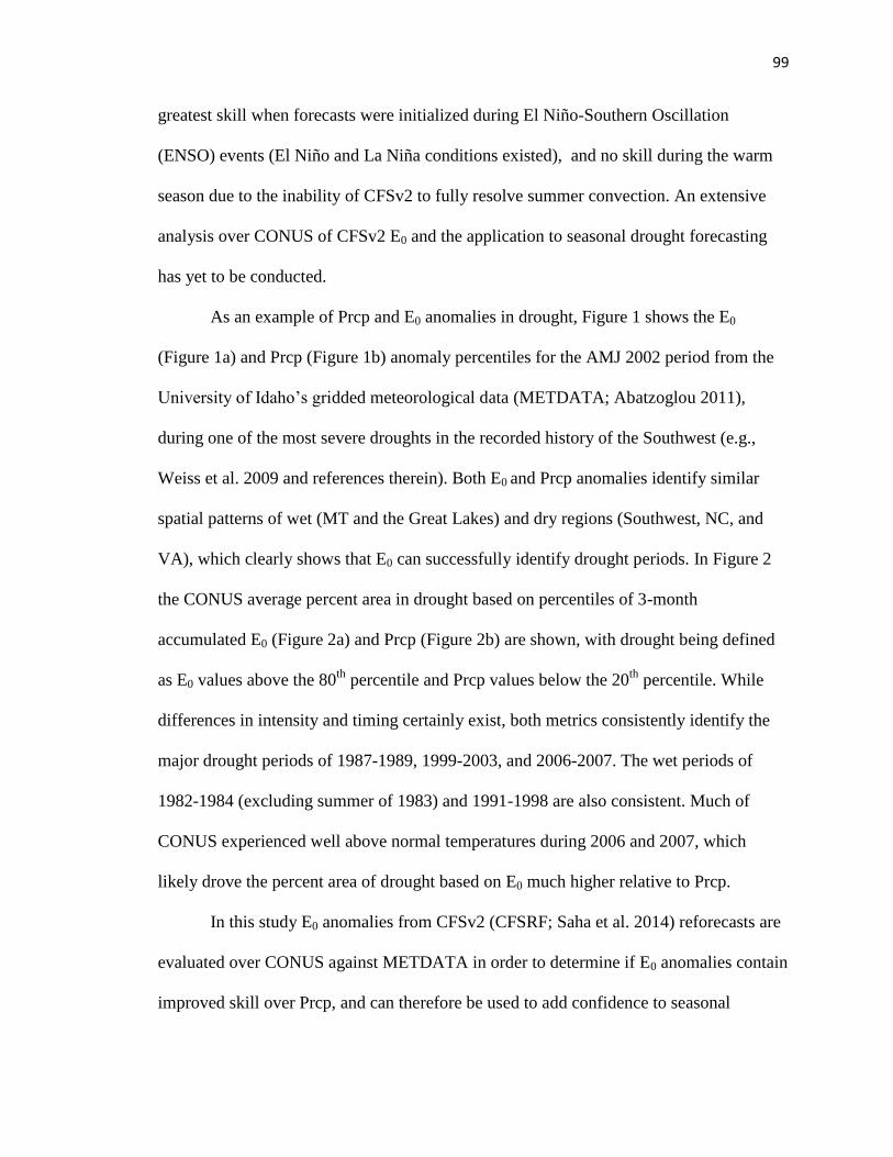
99

greatest skill when forecasts were initialized during El Niño-Southern Oscillation

(ENSO) events (El Niño and La Niña conditions existed), and no skill during the warm

season due to the inability of CFSv2 to fully resolve summer convection. An extensive

analysis over CONUS of CFSv2 E0 and the application to seasonal drought forecasting

has yet to be conducted.

As an example of Prcp and E0 anomalies in drought, Figure 1 shows the E0

(Figure 1a) and Prcp (Figure 1b) anomaly percentiles for the AMJ 2002 period from the

University of Idaho’s gridded meteorological data (METDATA; Abatzoglou 2011),

during one of the most severe droughts in the recorded history of the Southwest (e.g.,

Weiss et al. 2009 and references therein). Both E0 and Prcp anomalies identify similar

spatial patterns of wet (MT and the Great Lakes) and dry regions (Southwest, NC, and

VA), which clearly shows that E0 can successfully identify drought periods. In Figure 2

the CONUS average percent area in drought based on percentiles of 3-month

accumulated E0 (Figure 2a) and Prcp (Figure 2b) are shown, with drought being defined

as E0 values above the 80th

percentile and Prcp values below the 20th

percentile. While

differences in intensity and timing certainly exist, both metrics consistently identify the

major drought periods of 1987-1989, 1999-2003, and 2006-2007. The wet periods of

1982-1984 (excluding summer of 1983) and 1991-1998 are also consistent. Much of

CONUS experienced well above normal temperatures during 2006 and 2007, which

likely drove the percent area of drought based on E0 much higher relative to Prcp.

In this study E0 anomalies from CFSv2 (CFSRF; Saha et al. 2014) reforecasts are

evaluated over CONUS against METDATA in order to determine if E0 anomalies contain

improved skill over Prcp, and can therefore be used to add confidence to seasonal

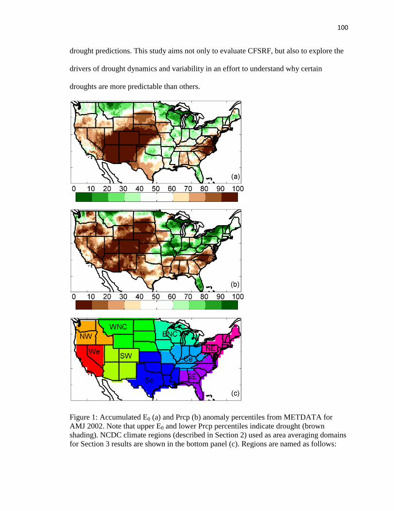
100

drought predictions. This study aims not only to evaluate CFSRF, but also to explore the

drivers of drought dynamics and variability in an effort to understand why certain

droughts are more predictable than others.

Figure 1: Accumulated E0 (a) and Prcp (b) anomaly percentiles from METDATA for

AMJ 2002. Note that upper E0 and lower Prcp percentiles indicate drought (brown

shading). NCDC climate regions (described in Section 2) used as area averaging domains

for Section 3 results are shown in the bottom panel (c). Regions are named as follows:

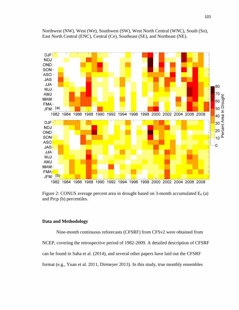
101

Northwest (NW), West (We), Southwest (SW), West North Central (WNC), South (So),

East North Central (ENC), Central (Ce), Southeast (SE), and Northeast (NE).

Figure 2: CONUS average percent area in drought based on 3-month accumulated E0 (a)

and Prcp (b) percentiles.

Data and Methodology

Nine-month continuous reforecasts (CFSRF) from CFSv2 were obtained from

NCEP, covering the retrospective period of 1982-2009. A detailed description of CFSRF

can be found in Saha et al. (2014), and several other papers have laid out the CFSRF

format (e.g., Yuan et al. 2011, Dirmeyer 2013). In this study, true monthly ensembles

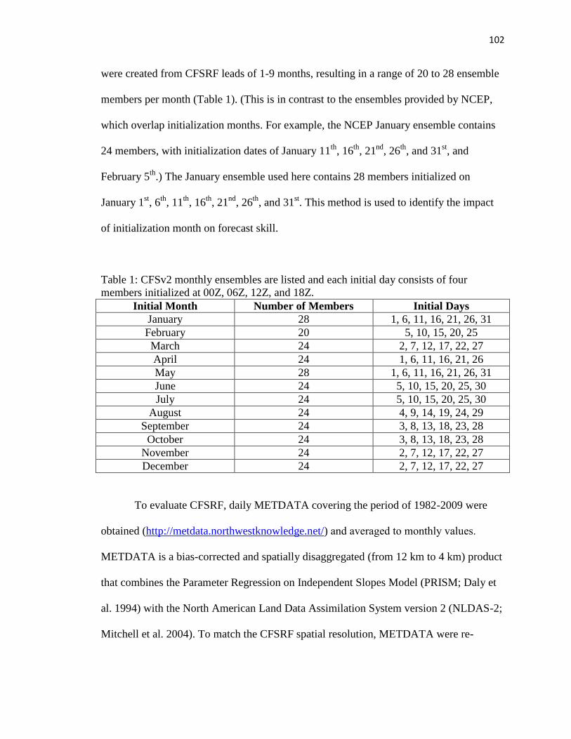
102

were created from CFSRF leads of 1-9 months, resulting in a range of 20 to 28 ensemble

members per month (Table 1). (This is in contrast to the ensembles provided by NCEP,

which overlap initialization months. For example, the NCEP January ensemble contains

24 members, with initialization dates of January 11th

, 16th

, 21nd

, 26th

, and 31st, and

February 5th

.) The January ensemble used here contains 28 members initialized on

January 1st, 6

th, 11

th, 16

th, 21

nd, 26

th, and 31

st. This method is used to identify the impact

of initialization month on forecast skill.

Table 1: CFSv2 monthly ensembles are listed and each initial day consists of four

members initialized at 00Z, 06Z, 12Z, and 18Z.

Initial Month Number of Members Initial Days

January 28 1, 6, 11, 16, 21, 26, 31

February 20 5, 10, 15, 20, 25

March 24 2, 7, 12, 17, 22, 27

April 24 1, 6, 11, 16, 21, 26

May 28 1, 6, 11, 16, 21, 26, 31

June 24 5, 10, 15, 20, 25, 30

July 24 5, 10, 15, 20, 25, 30

August 24 4, 9, 14, 19, 24, 29

September 24 3, 8, 13, 18, 23, 28

October 24 3, 8, 13, 18, 23, 28

November 24 2, 7, 12, 17, 22, 27

December 24 2, 7, 12, 17, 22, 27

To evaluate CFSRF, daily METDATA covering the period of 1982-2009 were

obtained (http://metdata.northwestknowledge.net/) and averaged to monthly values.

METDATA is a bias-corrected and spatially disaggregated (from 12 km to 4 km) product

that combines the Parameter Regression on Independent Slopes Model (PRISM; Daly et

al. 1994) with the North American Land Data Assimilation System version 2 (NLDAS-2;

Mitchell et al. 2004). To match the CFSRF spatial resolution, METDATA were re-

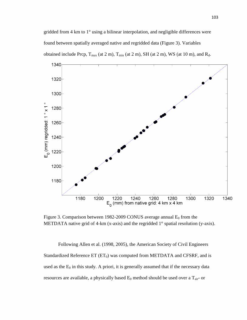
http://metdata.northwestknowledge.net/

103

gridded from 4 km to 1° using a bilinear interpolation, and negligible differences were

found between spatially averaged native and regridded data (Figure 3). Variables

obtained include Prcp, Tmax (at 2 m), Tmin (at 2 m), SH (at 2 m), WS (at 10 m), and Rd.

Figure 3. Comparison between 1982-2009 CONUS average annual E0 from the

METDATA native grid of 4-km (x-axis) and the regridded 1° spatial resolution (y-axis).

Following Allen et al. (1998, 2005), the American Society of Civil Engineers

Standardized Reference ET (ET0) was computed from METDATA and CFSRF, and is

used as the E0 in this study. A priori, it is generally assumed that if the necessary data

resources are available, a physically based E0 method should be used over a Tair- or

104

radiation- based method. Hobbins et al. (2012) and Hobbins (2015) demonstrated that

the dominant drivers of E0 variability change across CONUS depending on factors such

as aggregation period (monthly vs. annual) and season, and is not always Tair. For

example, during the summer WS is the dominant driver over much of the Great Basin,

while Rd dominates over much of the southeast CONUS. For ET0 computations at the

daily time step the soil heat flux (G) is assumed to zero. However, at monthly time steps

G must be calculated to account for warming and cooling of the soil in spring and

autumn, respectively. Following Allen et al. (1998; equations 43 and 44) mean monthly

Tair was used to calculate G. ET0 was first calculated for each ensemble member, and the

ensemble mean ET0 was then calculated.

A skill analysis was carried out over CONUS, and area averaging domains were

constructed using the nine National Climatic Data Center (NCDC) climate regions

(Figure 1c; Karl and Koss 1984). Monthly METDATA anomalies were computed relative

to the 1982-2009 METDATA mean. Following the recommendation of Kumar et al.

(2014), monthly CFSRF anomalies were calculated relative to the CFSRF climatology

(1982-2009) from the corresponding initialization month and lead time. Season 1

forecasts were generated as the accumulated anomaly over the first three months (i.e.,

season 1 JFM forecasts were initialized in December, and represents the accumulated

anomaly over JFM).

To assess CFSRF general skill, anomaly correlation (AC) between CFSRF

ensemble means and METDATA was computed for monthly one- to nine-month leads,

and season-1 forecasts, and is defined as follows:

105

𝐴𝐶 =(𝑓 − 𝑓𝑐)(𝑜 − 𝑜𝑐)̅̅ ̅̅ ̅̅ ̅̅ ̅̅ ̅̅ ̅̅ ̅̅ ̅̅ ̅̅ ̅̅

√(𝑓 − 𝑓𝑐)2̅̅ ̅̅ ̅̅ ̅̅ ̅̅ ̅̅ (𝑜 − 𝑜𝑐)2̅̅ ̅̅ ̅̅ ̅̅ ̅̅ ̅̅

where f is the forecast, fc is the forecast climatology, o is the observed value, and oc is

the observed climatology (Miyakoda et al. 1972; equation 11). Sample size for each AC

was 28 (number of reforecast years).

Skill during individual drought events was assessed based on the probability

forecasts, using the categorical Heidke skill score (HSS; O’Lenic et al. 2008) computed

over individual climate regions, and is defined as

𝐻𝑆𝑆 =(ℎ − 𝑒) ∗ 100

(𝑡 − 𝑒)

where h is the number of grid points with hits, or correct tercile forecast, t is the total

number of grid points, and e is the number of grid points expected to be correct by chance

(i.e., t/3).

All forecasts were used for the HSS, including grid points with “equal chances”,

following Peng et al. (2013).

Results

Deterministic skill

Figure 4 shows the spatially averaged monthly AC over each NCDC climate

region for ET0. Large regional and seasonal variability in skill was found, which indicates

that using only the CONUS average AC would not provide much valuable insight.

Maximum average AC for each region ranged from 0.41 (Southeast) to 0.66 (West). The

West, Southwest, and South regions all show a similar pattern of greatest skill during

January through June, with moderate skill (AC = 0.3 to 0.6) out to 5-months lead time,

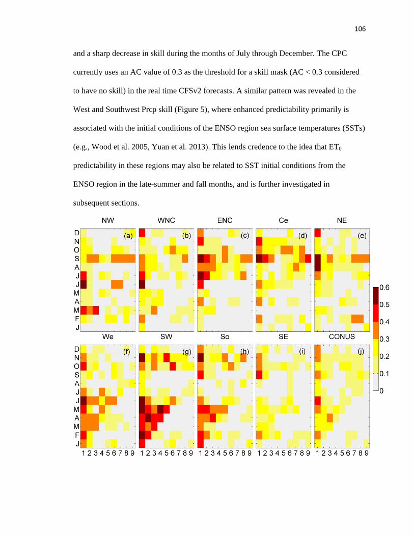
106

and a sharp decrease in skill during the months of July through December. The CPC

currently uses an AC value of 0.3 as the threshold for a skill mask (AC < 0.3 considered

to have no skill) in the real time CFSv2 forecasts. A similar pattern was revealed in the

West and Southwest Prcp skill (Figure 5), where enhanced predictability primarily is

associated with the initial conditions of the ENSO region sea surface temperatures (SSTs)

(e.g., Wood et al. 2005, Yuan et al. 2013). This lends credence to the idea that ET0

predictability in these regions may also be related to SST initial conditions from the

ENSO region in the late-summer and fall months, and is further investigated in

subsequent sections.

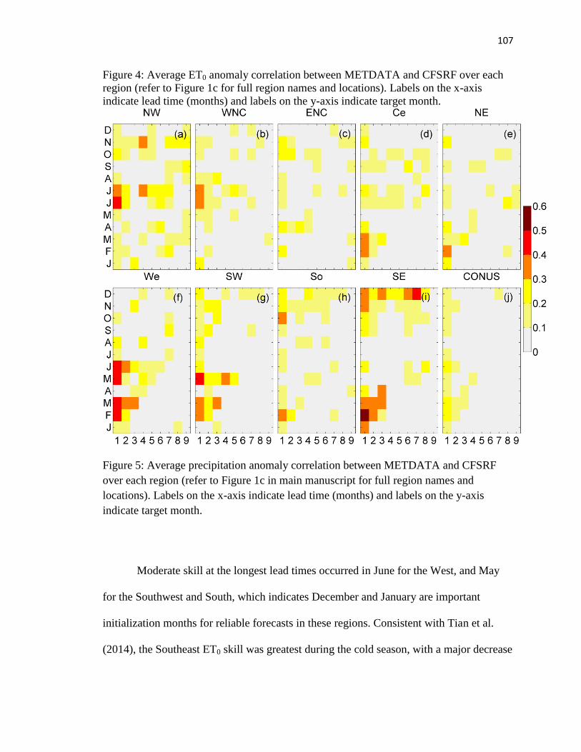
107

Figure 4: Average ET0 anomaly correlation between METDATA and CFSRF over each

region (refer to Figure 1c for full region names and locations). Labels on the x-axis

indicate lead time (months) and labels on the y-axis indicate target month.

Figure 5: Average precipitation anomaly correlation between METDATA and CFSRF

over each region (refer to Figure 1c in main manuscript for full region names and

locations). Labels on the x-axis indicate lead time (months) and labels on the y-axis

indicate target month.

Moderate skill at the longest lead times occurred in June for the West, and May

for the Southwest and South, which indicates December and January are important

initialization months for reliable forecasts in these regions. Consistent with Tian et al.

(2014), the Southeast ET0 skill was greatest during the cold season, with a major decrease

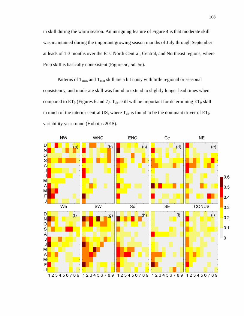
108

in skill during the warm season. An intriguing feature of Figure 4 is that moderate skill

was maintained during the important growing season months of July through September

at leads of 1-3 months over the East North Central, Central, and Northeast regions, where

Prcp skill is basically nonexistent (Figure 5c, 5d, 5e).

Patterns of Tmax and Tmin skill are a bit noisy with little regional or seasonal

consistency, and moderate skill was found to extend to slightly longer lead times when

compared to ET0 (Figures 6 and 7). Tair skill will be important for determining ET0 skill

in much of the interior central US, where Tair is found to be the dominant driver of ET0

variability year round (Hobbins 2015).

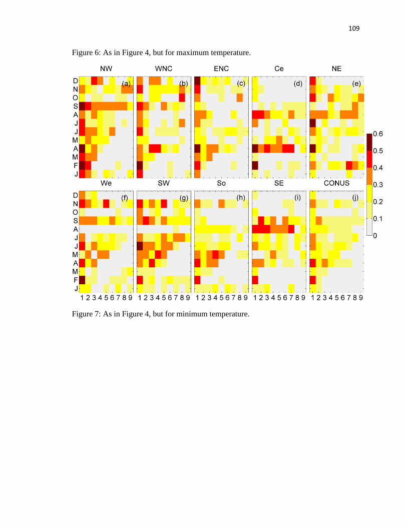
109

Figure 6: As in Figure 4, but for maximum temperature.

Figure 7: As in Figure 4, but for minimum temperature.

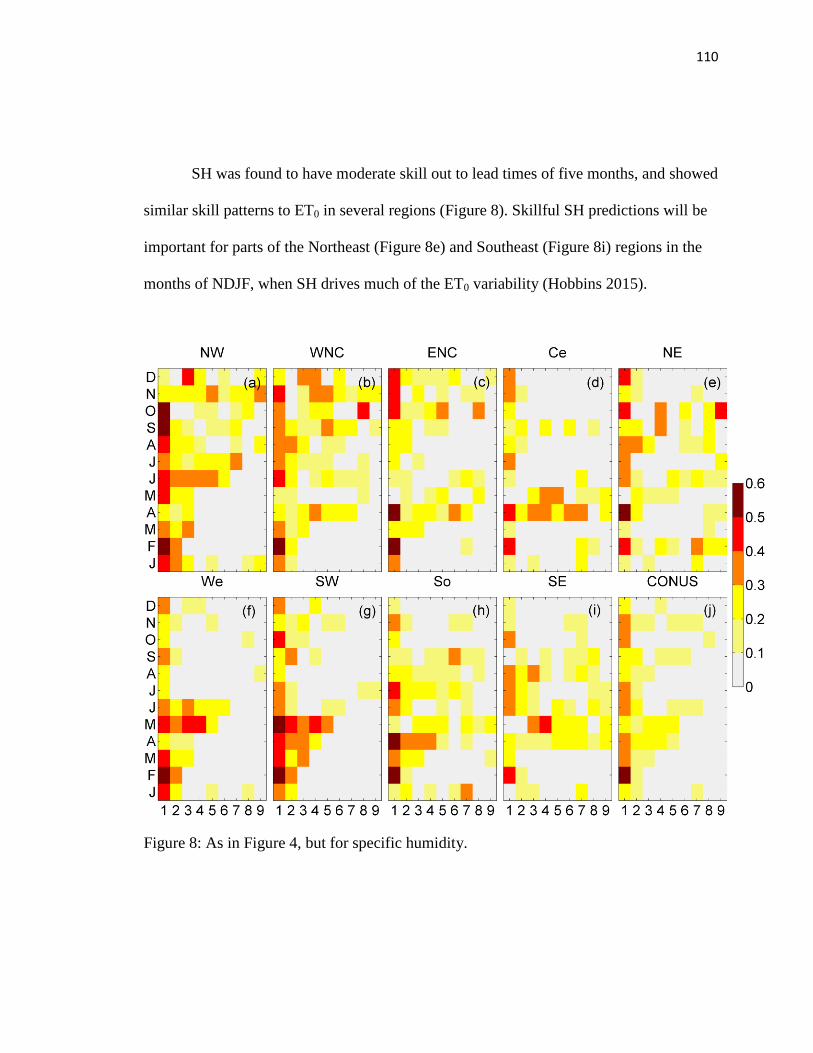
110

SH was found to have moderate skill out to lead times of five months, and showed

similar skill patterns to ET0 in several regions (Figure 8). Skillful SH predictions will be

important for parts of the Northeast (Figure 8e) and Southeast (Figure 8i) regions in the

months of NDJF, when SH drives much of the ET0 variability (Hobbins 2015).

Figure 8: As in Figure 4, but for specific humidity.

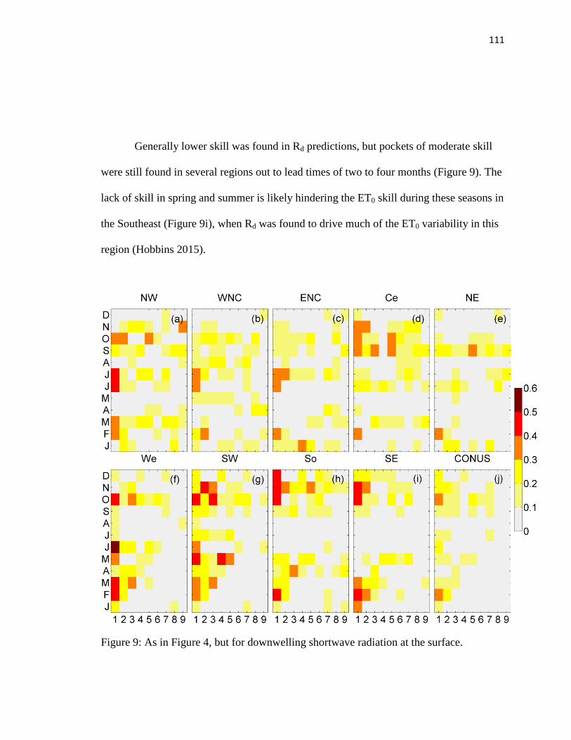
111

Generally lower skill was found in Rd predictions, but pockets of moderate skill

were still found in several regions out to lead times of two to four months (Figure 9). The

lack of skill in spring and summer is likely hindering the ET0 skill during these seasons in

the Southeast (Figure 9i), when Rd was found to drive much of the ET0 variability in this

region (Hobbins 2015).

Figure 9: As in Figure 4, but for downwelling shortwave radiation at the surface.

112

Wind speed forecasts were found to contain little usable skill (Figure 10), with the

exception of a few pockets with consistent AC of 0.3-0.4 in the Southwest (Figure 10g)

and South (Figure 10h) regions. Future improvements to WS predictions will be

important for improving ET0 skill in the Southwest and parts of the West during the

summer months, when WS controls much of the ET0 variability (Hobbins (2015).

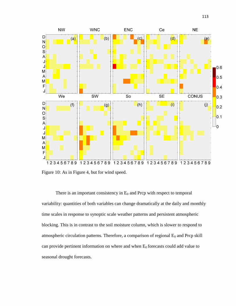
113

Figure 10: As in Figure 4, but for wind speed.

There is an important consistency in E0 and Prcp with respect to temporal

variability: quantities of both variables can change dramatically at the daily and monthly

time scales in response to synoptic scale weather patterns and persistent atmospheric

blocking. This is in contrast to the soil moisture column, which is slower to respond to

atmospheric circulation patterns. Therefore, a comparison of regional E0 and Prcp skill

can provide pertinent information on where and when E0 forecasts could add value to

seasonal drought forecasts.

114

Season 1 AC for both E0 and Prcp averaged over CONUS and its constituent nine

climate regions is shown in Figure 11. CONUS wide, E0 skill is greater than Prcp during

all seasons, and remains above the 0.3 AC threshold of moderate skill for more than half

of the year. Most regions contain at least one or two seasons when E0 skill exceeds Prcp

skill by ~0.2 to 0.5. Of particular interest are regions where E0 skill is high compared to

Prcp skill during the growing season, such as the East North Central, Central, and

Northeast. In these regions, enhanced reliability in seasonal drought forecasts could

greatly benefit agricultural operations during the heart of the growing season, as well as

harvest operations during the late summer and early fall. A second area of interest is in

the Southwest region, where moderate E0 skill during the fall, winter, and spring could

improve water supply outlooks, which is particularly important in UT and CO.

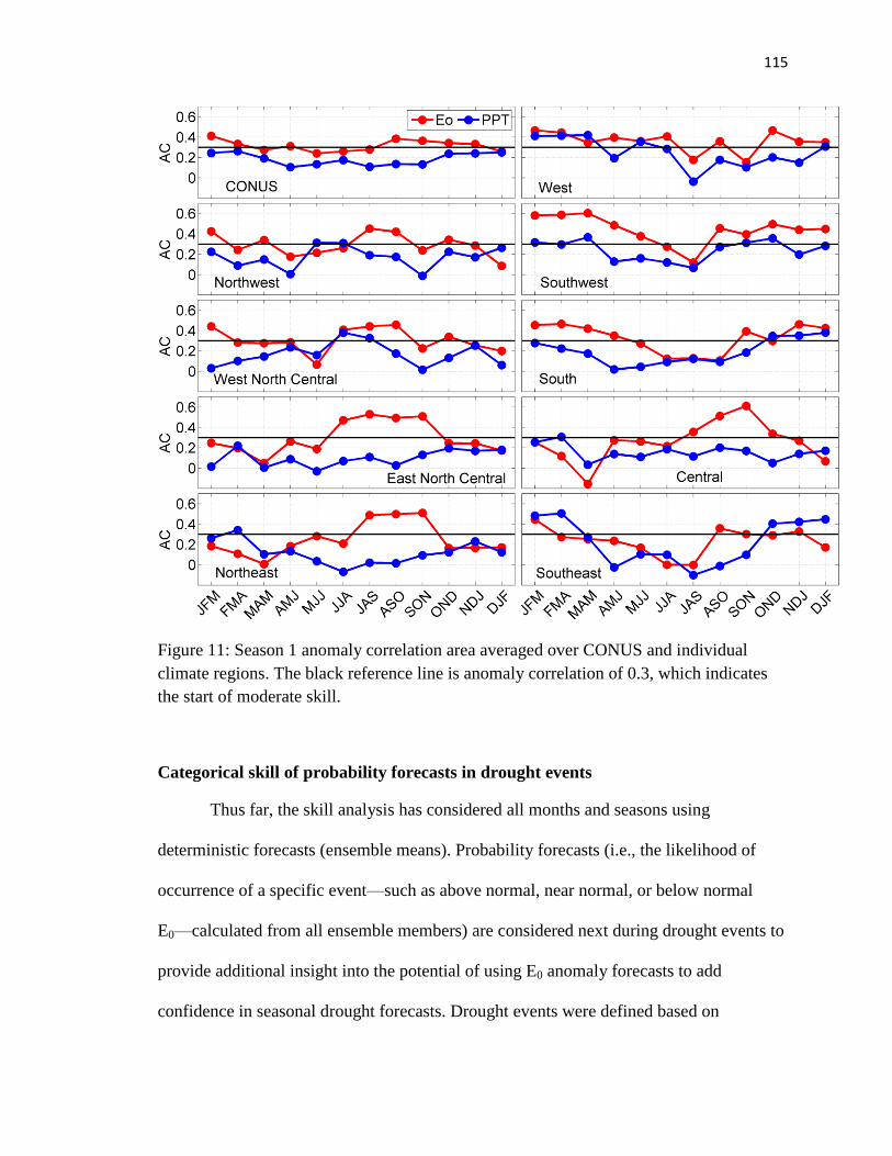
115

Figure 11: Season 1 anomaly correlation area averaged over CONUS and individual

climate regions. The black reference line is anomaly correlation of 0.3, which indicates

the start of moderate skill.

Categorical skill of probability forecasts in drought events

Thus far, the skill analysis has considered all months and seasons using

deterministic forecasts (ensemble means). Probability forecasts (i.e., the likelihood of

occurrence of a specific event—such as above normal, near normal, or below normal

E0—calculated from all ensemble members) are considered next during drought events to

provide additional insight into the potential of using E0 anomaly forecasts to add

confidence in seasonal drought forecasts. Drought events were defined based on

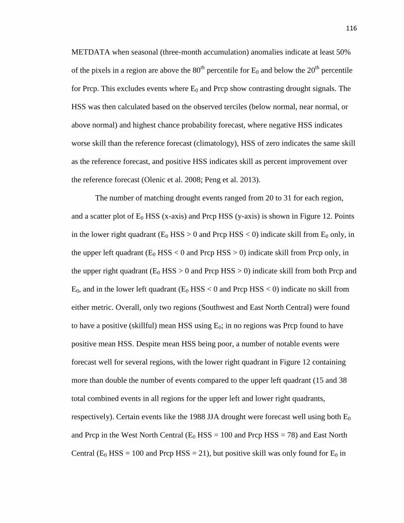
116

METDATA when seasonal (three-month accumulation) anomalies indicate at least 50%

of the pixels in a region are above the 80th

percentile for E0 and below the 20th

percentile

for Prcp. This excludes events where E0 and Prcp show contrasting drought signals. The

HSS was then calculated based on the observed terciles (below normal, near normal, or

above normal) and highest chance probability forecast, where negative HSS indicates

worse skill than the reference forecast (climatology), HSS of zero indicates the same skill

as the reference forecast, and positive HSS indicates skill as percent improvement over

the reference forecast (Olenic et al. 2008; Peng et al. 2013).

The number of matching drought events ranged from 20 to 31 for each region,

and a scatter plot of E0 HSS (x-axis) and Prcp HSS (y-axis) is shown in Figure 12. Points

in the lower right quadrant (E0 HSS > 0 and Prcp HSS < 0) indicate skill from E0 only, in

the upper left quadrant (E0 HSS < 0 and Prcp HSS > 0) indicate skill from Prcp only, in

the upper right quadrant (E0 HSS > 0 and Prcp HSS > 0) indicate skill from both Prcp and

E0, and in the lower left quadrant (E0 HSS < 0 and Prcp HSS < 0) indicate no skill from

either metric. Overall, only two regions (Southwest and East North Central) were found

to have a positive (skillful) mean HSS using E0; in no regions was Prcp found to have

positive mean HSS. Despite mean HSS being poor, a number of notable events were

forecast well for several regions, with the lower right quadrant in Figure 12 containing

more than double the number of events compared to the upper left quadrant (15 and 38

total combined events in all regions for the upper left and lower right quadrants,

respectively). Certain events like the 1988 JJA drought were forecast well using both E0

and Prcp in the West North Central (E0 HSS = 100 and Prcp HSS = 78) and East North

Central (E0 HSS = 100 and Prcp HSS = 21), but positive skill was only found for E0 in

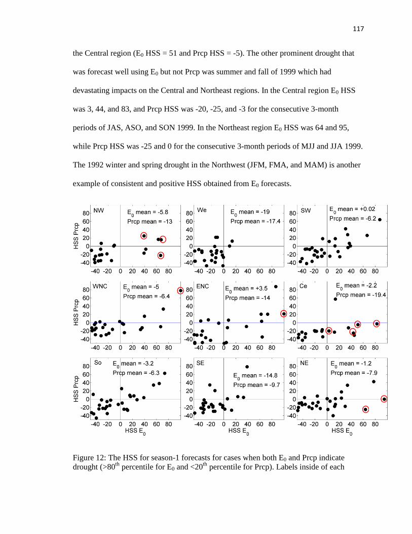
117

the Central region (E0 HSS = 51 and Prcp HSS = -5). The other prominent drought that

was forecast well using E0 but not Prcp was summer and fall of 1999 which had

devastating impacts on the Central and Northeast regions. In the Central region E0 HSS

was 3, 44, and 83, and Prcp HSS was -20, -25, and -3 for the consecutive 3-month

periods of JAS, ASO, and SON 1999. In the Northeast region E0 HSS was 64 and 95,

while Prcp HSS was -25 and 0 for the consecutive 3-month periods of MJJ and JJA 1999.

The 1992 winter and spring drought in the Northwest (JFM, FMA, and MAM) is another

example of consistent and positive HSS obtained from E0 forecasts.

Figure 12: The HSS for season-1 forecasts for cases when both E0 and Prcp indicate

drought (>80th

percentile for E0 and <20th

percentile for Prcp). Labels inside of each

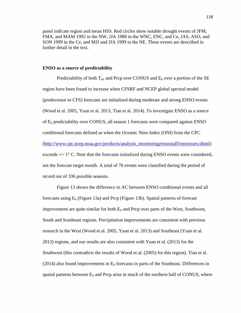
118

panel indicate region and mean HSS. Red circles show notable drought events of JFM,

FMA, and MAM 1992 in the NW, JJA 1988 in the WNC, ENC, and Ce, JAS, ASO, and

SON 1999 in the Ce, and MJJ and JJA 1999 in the NE. These events are described in

further detail in the text.

ENSO as a source of predictability

Predictability of both Tair and Prcp over CONUS and E0 over a portion of the SE

region have been found to increase when CFSRF and NCEP global spectral model

(predecessor to CFS) forecasts are initialized during moderate and strong ENSO events

(Wood et al. 2005, Yuan et al. 2013, Tian et al. 2014). To investigate ENSO as a source

of E0 predictability over CONUS, all season 1 forecasts were compared against ENSO

conditional forecasts defined as when the Oceanic Nino Index (ONI) from the CPC

(http://www.cpc.ncep.noaa.gov/products/analysis_monitoring/ensostuff/ensoyears.shtml)

exceeds +/- 1° C. Note that the forecasts initialized during ENSO events were considered,

not the forecast target month. A total of 76 events were classified during the period of

record out of 336 possible seasons.

Figure 13 shows the difference in AC between ENSO conditional events and all

forecasts using E0 (Figure 13a) and Prcp (Figure 13b). Spatial patterns of forecast

improvement are quite similar for both E0 and Prcp over parts of the West, Southwest,

South and Southeast regions. Precipitation improvements are consistent with previous

research in the West (Wood et al. 2005, Yuan et al. 2013) and Southeast (Yuan et al.

2013) regions, and our results are also consistent with Yuan et al. (2013) for the

Southwest (this contradicts the results of Wood et al. (2005) for this region). Tian et al.

(2014) also found improvements in E0 forecasts in parts of the Southeast. Differences in

spatial patterns between E0 and Prcp arise in much of the northern half of CONUS, where

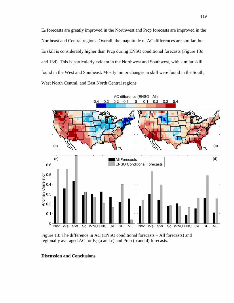
http://www.cpc.ncep.noaa.gov/products/analysis_monitoring/ensostuff/ensoyears.shtml

119

E0 forecasts are greatly improved in the Northwest and Prcp forecasts are improved in the

Northeast and Central regions. Overall, the magnitude of AC differences are similar, but

E0 skill is considerably higher than Prcp during ENSO conditional forecasts (Figure 13c

and 13d). This is particularly evident in the Northwest and Southwest, with similar skill

found in the West and Southeast. Mostly minor changes in skill were found in the South,

West North Central, and East North Central regions.

Figure 13: The difference in AC (ENSO conditional forecasts – All forecasts) and

regionally averaged AC for E0 (a and c) and Prcp (b and d) forecasts.

Discussion and Conclusions

120

We have provided the first CONUS wide study assessing seasonal predictions of

E0 anomalies using the CFSv2 reforecast (CFSRF) and METDATA observations. Nine

climate regions were used as area-averaging domains to assess regional skill variability.

Monthly ensemble mean forecasts were analyzed at one- to nine-month leads, and lead

one-month, season 1 ensemble mean forecasts were used to highlight seasonal skill

variability. Monthly E0 ACs revealed large regional and seasonal variability, with

moderate skill (AC of 0.3-0.6) found at one- to five-month leads but no consistent skill at

longer lead times.

Seasonal skill from E0 was found to be consistently greater than Prcp when

averaged over CONUS, and the same could be said for most regions where large AC

differences (0.2-0.5) were found depending on season. Assessment of probability

forecasts during drought using the HSS events revealed no skill on average, with the

exception of the Southwest and East North Central using E0. However, two of the most

severe warm-season droughts during the period of record (summer of 1988 and summer

and fall of 1999) and the winter and spring drought of 1992 in the Northwest were all

forecast with reasonable skill using E0 and mostly poor skill using Prcp. While it is still

unclear exactly what makes certain droughts predictable and others not, one prominent

feature of the 1988, 1992, and 1999 (Northeast only) events was high temperatures that

clearly exacerbated the E0 anomalies, and likely improved predictions over Prcp

forecasts. Another interesting finding is that a poor Prcp forecast would not necessarily

lead to a poor E0 forecast, which indicates a potential lack of land surface-atmospheric

coupling in CFSv2. These results indicate that including E0 anomalies in operational

seasonal drought forecasts could provide additional skill and boost overall confidence for

121

various applications such as water resource outlooks in regions that depend on seasonal

snow pack, and agricultural outlooks in the many important farming belts throughout

CONUS.

We have shown results that are consistent with previous research, and suggest that

some portion of E0 predictability comes from the initial state of tropical Pacific SSTs.

This is evident in the similar skill patterns found between E0 and Prcp in the West,

Southwest, and Southeast regions, where several studies have found enhanced Prcp and

Tair skill during strong ENSO events (e.g., Wood et al. 2005, Yuan et al. 2013), and in our

analysis of ENSO conditional vs. all events. Tian et al. (2014) also found enhanced E0

predictability when CFSv2 forecasts were initialized during ENSO events in the

Southeast cold season. Jia et al. (2015) found seasonal Prcp skill in a Geophysical Fluid

Dynamics Laboratory climate model to be mostly ENSO-related, but temperature skill to

be related to ENSO as well as changes in the external radiative forcings (i.e., a multi-

decadal warming signal in both summer and winter), which could be an additional factor

contributing to E0 skill from CFSv2. Initial state of the soil moisture column could also

be contributing to E0 predictability considering the ongoing feedbacks between the land

surface state and variables of Tmax, Tmin, and SH used to generate E0 estimates. Yuan et

al. (2013) found high skill in soil moisture forecasts at longer lead times and Yoon and

Leung (2015) found antecedent soil moisture to be as important as ENSO in seasonal

Prcp forecast skill over parts of CONUS.

This work also opens the door for continued research on improved skill in E0

seasonal forecasts via downscaling approaches (statistical or dynamical). Downscaling

was intentionally left out of this study to avoid masking CFSv2 deficiencies in E0 drivers

122

at the native grid scale. With the regional results that we have provided, it can be seen

that downscaling of E0 and most of the drivers (Tair, SH, and Rd), could be useful for local

applications other than drought forecasting, like irrigation water demands. However,

downscaling WS would likely not provide additional benefit given that poor skill was

found everywhere during all seasons. It may be useful to replace forecast WS with

climatological values, which has shown to improve skill in long-range weather forecasts

of E0 (Tian and Martinez 2012).

A multi-model ensemble, such as the NMME (North American Multi-Model

Ensemble; Kirtman et al. 2014), would certainly provide a more robust analysis then than

just considering CFSv2. However, at the time of writing, CFSv2 was the only seasonal

forecast model to provide publically available reforecasts of Rd, SH, and WS needed to

compute E0, while NMME Phase-I reforecasts only provide the Tair component needed

for E0. The NMME Phase-II data distribution is currently underway, which includes

output of all the required variables for E0 computations from seven seasonal forecast

models. Once NMME Phase-II data distribution is complete, a follow-up study will

establish whether E0 forecast skill can be enhanced using a multi-model ensemble

approach.

Skillful seasonal predictions remain a major challenge in drought forecasting, and

the use of E0 anomalies from CFSv2 clearly show potential improvements depending on

region and season. However, further research and improvements are needed for practical

use in an operational setting, and E0 and its drivers should continue to be evaluated in

other dynamical models as well as statistical techniques. Identifying systematic

consistencies in the physical mechanisms driving drought events where E0 shows good

123

skill and Prcp shows poor skill will also be a crucial step towards implementation of E0 in

a drought forecasting framework.

Acknowledgements

This research was supported by the Desert Research Institute (DRI) IBM PureSystems,

the Bureau of Reclamation Climate Analysis Tools WaterSMART program, and the

National Integrated Drought Information System (NIDIS).

References

Abatzoglou, J. T., 2011: Development of gridded surface meteorological data for

ecological

applications and modeling. Int. J. Climatol. 33, 121–131, DOI: 10.1002/joc.3413.

Anderson, M. C., C. R. Hain, B. Wardlow, J. R. Mecikalski, and W. P. Kustas, 2011:

Evaluation of a drought index based on thermal remote sensing of evapotranspiration

over the continental United States. J. Climate, 24, 2025–2044.

Hobbins, M. T., A. Wood, D. Streubel, and K. Werner, 2012: What drives the variability

of evaporative demand across the conterminous United States? J. Hydrometeor, 13,

1195–1214, doi: 10.1175/JHM-D-11-0101.1.

Karl T. R., and W. J. Koss, 1984: Regional and national monthly, seasonal, and annual

temperature weighted by area, 1895-1983. Historical Climatology Series 4-3,

National Climatic Data Center, Asheville, NC, 38 pp.

——, Gleason B. E., Menne M. J., 2012: US temperature and drought: recent anomalies

and trends. E0s Trans Am Geophys Union, 93, 473–474.

Kirtman, B. P., D. Min, J. M. Infanti, J. L. Kinter, III, D. A. Paolino, Q. Zhang, H. van

den Dool, S. Saha, M. P. Mendez, E. Becker, P. Peng, P. Tripp, J. Huang, D. G.

124

DeWitt, M. K. Tippett, A. G. Barnston, S. Li, A. Rosati, S. D. Schubert, M.

Rienecker, M. Suarez, Z. E. Li, J. Marshak, Y. Lim, J. Tribbia, K. Pegion, W. J. M.,

B. Denis, and E. F. Wood, 2014: The North American Multimodel Ensemble: Phase-

1 Seasonal-to-Interannual Prediction; Phase-2 toward Developing Intraseasonal

Prediction. Bull. Amer. Meteor. Soc., 95, 585–601.

doi: http://dx.doi.org/10.1175/BAMS-D-12-00050.1

Kumar, S., P. A. Dirmeyer, and J. L. Kinter III, 2014: Usefulness of ensemble forecasts

from NCEP Climate Forecast System in sub-seasonal to intra-annual forecasting,

Geophys. Res. Lett., 41, 3586–3593, doi:10.1002/2014GL059586.

Miyakoda, K., G. D., Hembree, R. F. Strickler, and I. Shulman, 1972: Cumulative results

of extended forecast experiments I. Model performance for winter cases. Mon. Wea.

Rev.100. 836-855.

Mu, Q., M. Zhao, J. S. Kimball, N. G. McDowell, S. W. Running, 2013: A remotely

sensed global terrestrial drought severity index. Bull. Amer. Meteor. Soc., 94, 93-98.

Otkin, J. A., M. C. Anderson, C. Hain, I. E. Mladenova, J. B. Basara, M. Svoboda, 2013:

Examining Rapid Onset Drought Development Using the Thermal Infrared–Based

Evaporative Stress Index. J. Hydrometeor., 14, 1057–1074.

Saha S., and coauthors, 2014: The NCEP Climate Forecast System Version 2. J. Climate,

27, 2185-2208. doi: http://dx.doi.org/10.1175/JCLI-D-12-00823.1.

Shukla, S., M. Safeeq, A. AghaKouchak, K. Guan, and C. Funk, 2015: Temperature

impacts on the water year 2014 drought in California. Geophys. Res. Lett., 42,

doi:10.1002/2015GL063666.

http://dx.doi.org/10.1175/BAMS-D-12-00050.1

http://dx.doi.org/10.1175/JCLI-D-12-00823.1

125

Tian, D., and C. J. Martinez, 2012: Forecasting reference evapotranspiration using

retrospective forecast analogs in the southeastern United States. J. Hydrometeor., 13,

1874–1892,

doi:10.1175/JHM-D-12-037.1.

Tian, D., C. J. Martinez, and W. D. Graham, 2014: Seasonal prediction of regional

reference evapotranspiration based on Climate Forecast System Version 2. J.

Hydrometeor., 15, 1166-1188. doi: http://dx.doi.org/10.1175/JHM-D-13-087.1.

Yao, Y., S. Liang, Q. Qin, K. Wang, 2010: Monitoring Drought over the Conterminous

United States Using MODIS and NCEP Reanalysis-2 Data. J. Appl. Meteor.

Climatol., 49, 1665–1680. doi: http://dx.doi.org/10.1175/2010JAMC2328.1

Yoon, J., and L. R. Leung, 2015: Assessing the relative influence of surface soil moisture

and ENSO SST on precipitation predictability over the contiguous United States.

Geophys. Res. Lett., doi: 10.1002/2015GL064139 (in press).

Yuan, X., E. F. Wood, L. Luo, and M. Pan, 2011: A first look at Climate Forecast System

version 2 (CFSv2) for hydrological seasonal prediction. Geophys. Res. Lett., 38,

doi:10.1029/2011GL047792.

——, E. F. Wood, J. K. Roundy, and M. Pan, 2013: CFSv2-based seasonal hydroclimatic

forecasts over the conterminous United States. J. Hydrometeor, 26, 4828-4847.

Weiss, J. L., C. L. Castro, and J. T. Overpeck, 2009: Distinguished pronounced droughts

in the Southwestern United States: seasonality and effects of warmer temperature. J.

Climate, 22, 5918-5932.

Wood, A. W., A. Kumar, and D. P. Lettenmaier, 2005: A retrospective assessment of

National Centers for Environmental Prediction climate model–based ensemble

http://dx.doi.org/10.1175/JHM-D-13-087.1

http://dx.doi.org/10.1175/2010JAMC2328.1

126

hydrologic forecasting in the western United States. J. Geophys. Res., 110, D04105,

doi:10.1029/2004JD004508.

Wood, E., S. Schubert, A. Wood, C. Peters-Lidard, K. Mo, A. Mariotti, and R. Pulwarty,

2015: Prospects for advancing drought understanding, monitoring and prediction. J.

Hydrometeor. doi:10.1175/JHM-D-14-0164.1, in press.

Xia, Y. and coauthors, 2012a: Continental-scale water and energy flux analysis and


(NLDAS-2): 1. Intercomparison and application of model products. J. Geophys Res.,

117 (D3), DOI: 10.1029/2011JD016048.

Xia, Y. and coauthors, 2012b: Continental-scale water and energy flux analysis and


(NLDAS-2): 2. Validation of model-simulated streamflow, J. Geophys Res., 117

(D3), DOI: 10.1029/2011JD016051.

127


Droughts are projected by global climate models to become more severe and

longer-lasting over portions of the US by the end of the 21st century, with drying

exacerbated by higher temperatures and increased evaporative demand (E0). Physically

based E0 has traditionally been neglected in drought monitoring, and there is a growing

need for the development of drought monitoring and forecasting methods and tools that

consider the effect of E0 and the drivers of E0 (temperature, humidity, wind speed, and

solar radiation) on drought development, intensification, and persistence.

Gridded data products (GDPs) are commonly used to estimate E0 without

thorough evaluation and understanding of biases and uncertainties in model

parameterizations. Several GDPs (PRISM, Daymet, and METDATA) were evaluated in

the Great Basin using a new observing network (independent of GDPs) in the Great

Basin—the Nevada Climate-Ecohydrological Assessment Network (NevCAN)—to

investigate the impact of terrain and GDP spatial resolution on estimates of precipitation,

temperature, and humidity.

Providing reliable “ground truth” for evaluating GDP precipitation estimates in

complex terrain was found to be challenging, with two co-located (~50 m apart) weather

stations (one dependent and one independent of GDPs) indicating about 30% difference

in water year precipitation totals. Nonetheless, GPDs were able to reproduce elevational

precipitation gradients, with a high bias (relative to NevCAN) in the cold season.

Temperatures were generally well replicated by GDPs with the exception of minimum

temperature (Tmin) at the alluvial fan locations. Nocturnal cold air drainage in complex

128

terrain results in large Tmin inversions at the alluvial fans (mean monthly lapse rates of >

+15°C km-1

were observed), which was captured by all GDPs (with the exception of

Daymet), but severely underestimated. This highlights the importance of using a non-

monotonic regression function, as in PRISM and METDATA, to estimate temperature.

Cold air pools and temperature inversions in complex terrain can lead to stagnant air and

long periods of poor air quality, and therefore spatially replicating this feature is of

utmost importance.

EDDI is the first drought indicator based solely on physically based E0 (the ASCE

Standardized Reference ET; ET0), and it was developed to fill a gap in monitoring of

drought dynamics driven by the aerodynamic (temperature, wind speed, and humidity)

and radiative (solar radiation and temperature) components of ET0. The Standardized

Precipitation Index (SPI), Standardized Soil Moisture Index (SSI), Evaporative Stress

Index (ESI), and United States Drought Monitor (USDM) were used to evaluate EDDI

across CONUS. The hypothesis was tested that EDDI can be a leading indicator during

rapid onset, or flash drought, due to both advective and radiative meteorological forcings

leading surface moisture depletion, and thus leading to a drought signal from EDDI prior

to other drought metrics. A sensitivity analysis on the drivers of EDDI during a flash

drought that transitioned to an extended drought revealed that it was high wind speed and

low humidity that initiated the flash drought, and extreme temperatures acted to

exacerbate the severity of EDDI and maintain an extended drought signal even during

periods of normal to slightly above normal precipitation. This reinforces the idea that a

temperature is not always the dominant driver of ET0 variability, especially at short time

129

scales, and temperature-based E0 cannot be used to capture realistic dynamics of flash

drought development.

Providing reliable seasonal drought forecasts remains a major challenge, and the

results from Chapter 2 motivated a study on the use of ET0 anomalies as a tool to

improve and add confidence to seasonal drought forecasts. Seasonal precipitation

forecasts hold little skill past the range of weather (~two weeks), with temperature

showing improved skill out to several months. Therefore, ET0 forecasts, with temperature

as an input, should be more skillful than precipitation. However, little is known about the

skill of seasonal humidity, solar radiation, and wind speed forecasts; the other drivers of

ET0 that can dominate the variability depending on season and region. In Chapter 3

reforecasts of ET0 and precipitation anomalies from the Climate Forecast System Version

2 (CFSv2) were evaluated against METDATA for the period of 1982-2009 over CONUS.

Forecasts of the individual drivers of ET0 were also evaluated. While overall probabilistic

skill of drought events was rather low, the severe warm-season droughts of 1988 and

1999 in the central and northeast US and the spring drought of 1992 in the Pacific

Northwest were all forecast with moderate skill using ET0.

The results presented in this dissertation can be useful to a number of groups both

in the scientific community and general public, and the conclusions and

recommendations are as follows:

Finer GDP spatial resolution does not always lead to less error when compared to

observations, and GDP performance varied greatly depending on region and

130

climate variable. It is strongly recommended that local analysis be conducted

prior to GDP use in hydro-climatic applications.

Using an over-simplified method to estimate dew point temperature (Tdew) in

Daymet—i.e., that daily average Tdew can be estimated as daily Tmin—is

unacceptable in semiarid to arid regions; this finding is particularly important

when considering GDPs for physically based E0 estimates.

METDATA is recommended for ET0 and EDDI calculations, with more realistic

humidity estimates compared to Daymet.

The hypothesis is confirmed that using a short time scale EDDI (two weeks to one

month) can be useful as an early warning indicator during flash drought

conditions, and EDDI was found to lead other indicators, such as SPI, SSI, and

the USDM, by up to three months.

EDDI could greatly benefit the agricultural, water resources, public health, and

recreation sectors through reactive emergency responses and implementation of

action plans in a timely manner.

EDDI can be useful to monitor hydrologic drought at longer time scales (6-12

months) in water-limited regions, which can be explained by the complementary

relationship between ET and ET0.

Seasonal forecasts of ET0 consistently contained greater skill than precipitation

relative to METDATA observations, with the greatest improvement found in parts

of the central and northeast US during the growing season, when precipitation

skill is nearly nonexistent.

131

Seasonal forecasts of ET0 anomalies may be particularly useful for increasing

confidence in season one outlooks during severe droughts driven by high

temperatures.

ET0 seasonal forecast skill is greatly enhanced in the northwest, west, southwest,

and southeast CONUS when forecasts are initialized during moderate and strong

El Niño-Southern Oscillation events.

Currently, EDDI is being updated in near real time (2-4 day latency), and continued

efforts should incorporate EDDI in operational drought-monitoring activities such as the

USDM. Seasonal forecasts of ET0 anomalies may be most beneficial to agricultural

sectors in the central and northeast US. Development of real-time seasonal ET0 forecasts

using CFSv2 is currently in progress, and will be made publically available in the near

future.

Physically Based Evaporative Demand as a Drought Metric ... · Physically Based Evaporative Demand...

Documents

Transcript of Physically Based Evaporative Demand as a Drought Metric ... · Physically Based Evaporative Demand...