Physical Processes in the Vicinity of a Supermassive Black ...tdo/tdo_thesis.pdf · University of...

University of California

Los Angeles

Physical Processes in the Vicinity of a

Supermassive Black Hole

A dissertation submitted in partial satisfaction

of the requirements for the degree

Doctor of Philosophy in Astronomy

by

Tuan Do

2010

c© Copyright by

Tuan Do

2010

The dissertation of Tuan Do is approved.

Craig Manning

James Larkin

Mark Morris

Andrea Ghez, Committee Chair

University of California, Los Angeles

2010

ii

to Mom and Dad

iii

Table of Contents

1 Introduction . . . . . . . . . . . . . . . . . . . . . . . . . . . . . . . . 1

1.1 Laser guide star adaptive optics . . . . . . . . . . . . . . . . . . . 2

1.2 The near-infrared emission from Sgr A* . . . . . . . . . . . . . . . 3

1.3 Dynamical evolution of stars at the Galactic center . . . . . . . . 5

2 Near-IR variability of Sgr A*: a red noise source with no de-

tected periodicity . . . . . . . . . . . . . . . . . . . . . . . . . . . . . . 10

2.1 Observations and Data Reduction . . . . . . . . . . . . . . . . . . 13

2.2 Results and Analysis . . . . . . . . . . . . . . . . . . . . . . . . . 18

2.2.1 Flux Distribution . . . . . . . . . . . . . . . . . . . . . . . 18

2.2.2 Light Curves and Timing Analysis . . . . . . . . . . . . . 22

2.3 Discussion . . . . . . . . . . . . . . . . . . . . . . . . . . . . . . . 40

2.3.1 Comparisons with X-ray variability . . . . . . . . . . . . . 41

2.3.2 The effect of measurement noise on the inferred PSD slope 43

2.3.3 Limits on a quiescent state of Sgr A* . . . . . . . . . . . . 45

2.4 Conclusion . . . . . . . . . . . . . . . . . . . . . . . . . . . . . . . 47

3 High angular resolution integral-field spectroscopy of the Galaxy’s

nuclear cluster: a missing stellar cusp? . . . . . . . . . . . . . . . . . 49

3.1 Introduction . . . . . . . . . . . . . . . . . . . . . . . . . . . . . . 49

3.2 Observations . . . . . . . . . . . . . . . . . . . . . . . . . . . . . . 54

3.3 Data Reduction . . . . . . . . . . . . . . . . . . . . . . . . . . . . 57

iv

3.4 Spectral Identification . . . . . . . . . . . . . . . . . . . . . . . . 59

3.5 Results . . . . . . . . . . . . . . . . . . . . . . . . . . . . . . . . . 77

3.6 Discussion . . . . . . . . . . . . . . . . . . . . . . . . . . . . . . . 82

3.6.1 Mass segregation . . . . . . . . . . . . . . . . . . . . . . . 84

3.6.2 Envelope destruction by stellar collisions . . . . . . . . . . 85

3.6.3 IMBH or binary black hole . . . . . . . . . . . . . . . . . . 87

3.6.4 Prospects for future observations . . . . . . . . . . . . . . 88

3.7 Conclusions . . . . . . . . . . . . . . . . . . . . . . . . . . . . . . 89

4 Using kinematics to constrain the distribution of stars at the

Galactic center . . . . . . . . . . . . . . . . . . . . . . . . . . . . . . . . 91

4.1 Introduction . . . . . . . . . . . . . . . . . . . . . . . . . . . . . . 91

4.2 Limits on line-of-sight distance with velocities . . . . . . . . . . . 92

4.3 Limits on line-of-sight distance with accelerations . . . . . . . . . 93

4.4 Using velocity distributions . . . . . . . . . . . . . . . . . . . . . 97

4.4.1 The Plummer model . . . . . . . . . . . . . . . . . . . . . 100

4.4.2 Power law density profiles . . . . . . . . . . . . . . . . . . 103

4.4.3 An isotropic core model . . . . . . . . . . . . . . . . . . . 106

4.4.4 Beyond isotropic models . . . . . . . . . . . . . . . . . . . 109

4.5 Conclusion . . . . . . . . . . . . . . . . . . . . . . . . . . . . . . . 109

5 Conclusions . . . . . . . . . . . . . . . . . . . . . . . . . . . . . . . . 111

5.1 Prospects for clarifying the nature of Sgr A*-IR . . . . . . . . . . 112

5.2 Origin of the missing stellar cusp . . . . . . . . . . . . . . . . . . 113

v

A OSIRIS wavelength calibrations . . . . . . . . . . . . . . . . . . . 115

A.1 Characterizing the wavelength shifts . . . . . . . . . . . . . . . . 115

B Catalog of OSIRIS spectra . . . . . . . . . . . . . . . . . . . . . . . 119

vi

List of Figures

1.1 NIR color magnitude diagram of the GC . . . . . . . . . . . . . . 9

2.1 Sgr A* and photometric reference sources . . . . . . . . . . . . . . 15

2.2 Noise statistics . . . . . . . . . . . . . . . . . . . . . . . . . . . . 17

2.3 Sgr A* flux density distribution . . . . . . . . . . . . . . . . . . . 18

2.4 Distribution of Sgr A* flux at L′ . . . . . . . . . . . . . . . . . . . 20

2.5 Nightly flux of Sgr A* and comparison source . . . . . . . . . . . 21

2.6 K ′ light curves of Sgr A* and S0-17 . . . . . . . . . . . . . . . . . 24

2.7 L′ light curves of Sgr A* and S0-2 . . . . . . . . . . . . . . . . . . 25

2.8 Lomb-Scargle periodograms of the Sgr A* K ′ light curves . . . . . 29

2.9 Averaged Sgr A* periodogram . . . . . . . . . . . . . . . . . . . . 30

2.10 Periodograms of reference sources . . . . . . . . . . . . . . . . . . 32

2.11 Simulations of QPO signals . . . . . . . . . . . . . . . . . . . . . 33

2.12 Statistical test for QPOs with the light curve observed on 2003

Jun 16 with VLT . . . . . . . . . . . . . . . . . . . . . . . . . . . 34

2.13 The structure functions for the K ′ light curves for Sgr A* and S0-17 36

2.14 Structure function for Sgr A* and S2-133 . . . . . . . . . . . . . . 37

2.15 L′ Structure function for Sgr A* and S0-2 . . . . . . . . . . . . . 39

2.16 Relationship between intrinsic PSD power index and measured

structure function . . . . . . . . . . . . . . . . . . . . . . . . . . . 40

2.17 Dependence of measured power law slopes on noise level . . . . . 44

vii

3.1 The currently surveyed region overlaid on a K′ (2.2 µm) image

of the Galactic center taken in 2007. Sgr A* is marked at the

center with a *. Spectroscopically identified early (blue triangles)

and late-type (red circles) stars are marked. Each field is enclosed

by dotted lines. Some spectral identifications are outside of the

marked lines because they were found at the edge of the dithers. . 56

3.2 Example of observed spectra in the Kn3 narrowband wavelength

region of early and late-type stars. The Br γ and Na I lines are

used to differentiate between early and late-type stars, respectively.

S0-2 is a K ′ = 14.1 early-type star with a strong Br γ line. S2-74

is a K ′ = 13.3 early-type star showing a featureless spectrum in

the OSIRIS Kn3 filter wavelength range. S0-13 is a K ′ = 13.5 late-

type star showing the Na I doublet. See Figures 2a, 2b, and 2c in

Appendix ?? for the spectra of all stars with spectral identification. 60

3.3 The relationship between the SNR and K ′ for stars observed in

this study and their spectral type. The spectral types of every

star with SNR > 40 was determined successfully. . . . . . . . . . . 62

3.4 Top: equivalent width of the combination of Na I lines at 2.2062

and 2.2090 µm as a function of K ′ magnitude. Also plotted are

equivalent width measurements of Na I from Forster Schreiber

(2000) with spectral types corrected for the distance and extinction

(Ak=3.0) toward the Galactic center (red). Bottom: equivalent

width of the Br γ hydrogen line at 2.1661 µm. Equivalent width

measurements from Hanson et al. (1996) are also plotted for O and

B type stars, corrected for the distance and extinction (Ak=3.0)

to the Galactic center (red). . . . . . . . . . . . . . . . . . . . . . 63

viii

3.5 The K ′ luminosity function from the spectroscopic survey in com-

parison to that found from imaging. In the top plot, we also include

for reference, the rough spectral types expected to be observable

at each luminosity bin assuming AK = 3.0 and a distance of 8 kpc.

The axis on the right shows the H-K color associated with each

of the spectral types (Ducati et al., 2001; Martins & Plez, 2006).

The WR stars occupy a range in both K ′ and H-K colors. . . . . 64

3.6 The K ′ luminosity function from the spectroscopic survey in com-

parison to imaging in each individual pointing. . . . . . . . . . . 65

3.7 Images from collapsing the OSIRIS data cubes along the spectral

dimension for each individual pointing of the survey. Right: me-

dian of all spectral channels. Left: spectral channels near the Br

gamma line showing the gas emission. The images are oriented

with north up and east to the left. Spectroscopically identified

early (blue triangles) and late-type (red circles) stars are marked. 66

3.8 Similar to Figure 3.7, with additional OSIRIS fields. . . . . . . . . 67




3.12 Plot of the surface number density as a function of projected dis-

tance from Sgr A* in the plane of the sky for different populations:

old (late-type, red), young (early-type, blue), and total number

counts from K ′ imaging. . . . . . . . . . . . . . . . . . . . . . . . 78

ix

3.13 Plot of the surface number density as a function of projected dis-

tance from Sgr A* in the plane of the sky for different populations:

old (late-type, red), young (early-type, blue), and total number

counts from K ′ imaging. These radial profiles have been corrected

for completeness and extinction using the method detailed in Sec-

tion 3.5. . . . . . . . . . . . . . . . . . . . . . . . . . . . . . . . . 81

3.14 Left: broken power law density profiles with break radius, rbreak =

8.0′′ and outer power law γ2 = 2.0, and varying inner power laws

γ1. Right: the projected surface number density profile of each of

the broken power laws. The fitted inner surface density power law

Γ is flat for γ1 ∼< 0.5. . . . . . . . . . . . . . . . . . . . . . . . . . 83

3.15 Left: the results of the Monte Carlo simulations of different inner

radial power laws γ and the resulting measured projected power

law of the radial profile, Γ = −0.26 ± 0.24. Center: using our

measurements, we can constrain some of the parameter space for

Γ vs. γ. Right: we marginalize over Γ to determine that our

measurement constrains γ to be less than 1.0 at a 99.7% confidence

level. . . . . . . . . . . . . . . . . . . . . . . . . . . . . . . . . . . 85

4.1 Diagram of acceleration components. . . . . . . . . . . . . . . . . 93

4.2 Values of a2D as a function of z distances for different projected

R2d distances. . . . . . . . . . . . . . . . . . . . . . . . . . . . . . 94

4.3 Values of a2D as a function of R2D distances for different z distances. 95

4.4 Values of az as a function of z distances for different projected R2d

distances. . . . . . . . . . . . . . . . . . . . . . . . . . . . . . . . 96

4.5 Values of az as a function of R2D distances for different z distances. 96

x

4.6 Location of line-of-sight distances that can be detected for stars

based on the typical acceleration errors. . . . . . . . . . . . . . . . 98

4.7 F (R, v) for the Plummer Model . . . . . . . . . . . . . . . . . . . 102

4.8 F (R, vz) for the Plummer Model . . . . . . . . . . . . . . . . . . . 102

4.9 P (R, < v) for the Plummer model . . . . . . . . . . . . . . . . . . 104

4.10 P (R, < v) for a cusp model . . . . . . . . . . . . . . . . . . . . . 106

4.11 An isotropic core model . . . . . . . . . . . . . . . . . . . . . . . 107

4.12 P (R, < v) for a cusp model . . . . . . . . . . . . . . . . . . . . . 108

A.1 OSIRIS wavelength shifts 2006-2009 in Kn3 . . . . . . . . . . . . 118

B.1 Early-type stars with Br gamma lines in Kn3, shifted to rest wave-

length and grouped by OSIRIS field location. . . . . . . . . . . . . 120

B.2 Continuation of Figure B.1 . . . . . . . . . . . . . . . . . . . . . . 121









B.11 Early-type stars with featureless spectra in Kn3, shifted to rest

wavelength and grouped by OSIRIS field location. . . . . . . . . . 130

xi

B.12 Continuation of Figure B.11. . . . . . . . . . . . . . . . . . . . . . 131



B.15 Late-type stars in Kn3, shifted to rest wavelength and grouped by

OSIRIS field location. . . . . . . . . . . . . . . . . . . . . . . . . . 134


















xii

List of Tables

2.1 Summary of Observations of Sgr A* . . . . . . . . . . . . . . . . . 14

2.2 PSD fits from the structure function . . . . . . . . . . . . . . . . 39

3.1 Summary of OSIRIS observations . . . . . . . . . . . . . . . . . . 55

3.2 OSIRIS observations of late-type stars . . . . . . . . . . . . . . . 71



3.3 OSIRIS observations of early-type stars . . . . . . . . . . . . . . . 74



3.4 OSIRIS spectra with unknown spectral type . . . . . . . . . . . . 76

3.4 OSIRIS spectra with unknown spectral type . . . . . . . . . . . . 77

3.5 Results and survey completeness . . . . . . . . . . . . . . . . . . . 79

3.6 Field Completeness . . . . . . . . . . . . . . . . . . . . . . . . . . 80

3.7 Extinction Corrected Field Completeness . . . . . . . . . . . . . . 80

A.1 OH lines used for refining the wavelength calibration in the Kn3

filter . . . . . . . . . . . . . . . . . . . . . . . . . . . . . . . . . . 116

xiii

Acknowledgments

This thesis could not have been written in isolation. Many people in all parts of

my life have made essential contributions to its completion. I would like to thank

my advisor, Andrea Ghez for helping me become a better scientist; Mark Morris

for illuminating discussions; Shelley Wright and James Larkin for teaching me

all I know about integral field spectroscopy; Brad Hansen and Matthew Wood

for discussions of stellar kinematic models; Xi Chen, Sylvana Yelda, Damien

Ramunno-Johnson, and Quinn Konopacky for your support throughout grad

school. Most of all, I would like to thank my father, mother, and brother for

their lifelong support of my education.

I acknowledge that results presented in this thesis are based on published

works with additional coauthors. In particular, Chapter two is a version of Do

et al. (2009b) and Chapter Three is derived from Do et al. (2009a). The W.M.

Keck Observatory is operated as a scientific partnership among the California

Institute of Technology, the University of California and the National Aeronautics

and Space Administration. The Observatory was made possible by the generous

financial support from the W. M. Keck Foundation.

xiv

Vita

1982 Born, Vietnam

2004 B.A. (Astrophysics, Physics)University of California, Berkeley

2006 M.S. (Astronomy)University of California, Los Angeles.

Publications

Stolte, A., Morris, M. R., Ghez, A. M., Do, T., Lu, J. R., Ballard, C., Mills, E.,Matthews, K., “Disks in the Arches cluster – survival in a starburst environment”,2010, The Astrophysical Journal, 718, 801

Do, T., Ghez, A. M., Morris, M. R., Lu, J. R., Matthews, K., Yelda, S., Larkin, J.,2009, “High angular resolution integral-field spectroscopy of the Galaxy’s nuclearcluster: a missing stellar cusp?”, The Astrophysical Journal, 703, 1323

Meyer, L., Do, T., Ghez, A., Morris, M. R., Yelda, S., Schoedel, R., Eckart, A.,“A power-law break in the near-infrared power spectrum of the Galactic centerblack hole”, 2009, The Astrophysical Journal Letters, 694, 1

Do, T., Ghez, A. M., Morris, M. R., Yelda, S., Meyer, L., Lu, J. R., Hornstein, S.D., Matthews, K., “A Near-Infrared Variability Study of the Galactic Black Hole:A Red Noise Source with No Detected Periodicity”, 2009, The AstrophysicalJournal, 691, 1021

Ghez, A. M., Salim, S., Weinberg, N. N., Lu, J. R., Do, T., Dunn, J. K.,Matthews, K., Morris, M. R., Yelda, S., Becklin, E. E., Kremenek, T., Milosavl-jevic, M., Naiman, J., “Measuring Distance and Properties of the Milky Way’s

xv

Central Supermassive Black Hole with Stellar Orbits”, 2008, The AstrophysicalJournal, 689, 1044

Meyer, L., Do, T., Ghez, A., Morris, M. R., Witzel, G., Eckart, A., Blanger, G.,Schodel, R., “A 600 Minute Near-Infrared Light Curve of Sagittarius A*”, 2008,ApJL, 688, 17

Do, T., Ghez, A. M., Morris, M. R., Yelda, S., Lu, J. R., Hornstein, S. D.,Matthews, K., “Testing for periodicities in near-IR light curves of Sgr A*”, 2008,Journal of Physics: Conference Series, Volume 131, Proceedings of “The UniverseUnder the Microscope - Astrophysics at High Angular Resolution”

Do, T., Morris, M. R., Sahai, R., Stapelfeldt, K., “A Spitzer Study of the Mass-Loss Histories of Three Bipolar Preplanetary Nebulae”, 2007, Astronomical Jour-nal, 134, 1417

Morris, M. R., Uchida, K., Do, T., “A magnetic torsional wave near the GalacticCentre traced by a double helix nebula”, 2006, Nature, 7082, 308

Hinkle, K. H., Joyce, R. R., Do, T., “Dust enshrouded AGB stars in the LMC”,2004, Variable Stars in the Local Group, IAU Colloquium 193, Conference Pro-ceedings

xvi

Abstract of the Dissertation

Physical Processes in the Vicinity of a

Supermassive Black Hole

by

Tuan Do

Doctor of Philosophy in Astronomy

University of California, Los Angeles, 2010

Professor Andrea Ghez, Chair

The Galactic center offers us an opportunity to study the environment around a

supermassive black hole at a level of detail not possible in other galactic nuclei.

This potential has been greatly expanded by the implementation of laser guide

star adaptive optics and integral field spectroscopy on large ground-based tele-

scopes. This thesis takes advantage of these technologies to address the nature

of the variable near-infrared emission from the black hole as well as test theories

of the equilibrium configuration of a star cluster with a supermassive black hole

at its center.

First, we present the results of near-infrared (2 and 3 µm) monitoring of Sgr

A*-IR with 1 min time sampling. Sgr A*-IR was observed continuously for up to

three hours on each of seven nights, between 2005 July and 2007 August. Sgr A*-

IR is detectable at all times and is continuously variable, with a median observed

2 µm flux density of 0.192 mJy, corresponding to 16.3 magnitude at K ′. These

observations allow us to investigate Nyquist sampled periods ranging from about

2 minutes to an hour. Using Monte Carlo simulations, we find that the variability

of Sgr A* in this data set is consistent with models based on correlated noise with

xvii

power spectra having frequency dependent power law slopes between 2.0 to 3.0,

consistent with those reported for AGN light curves. Of particular interest are

periods of ∼ 20 min, corresponding to a quasi-periodic signal claimed based upon

previous near-infrared observations and interpreted as the orbit of a ‘hot spot’

at or near the last stable orbit of a spinning black hole. We find no significant

periodicity at any time scale probed in these new observations for periodic signals.

This study is sensitive to periodic signals with amplitudes greater than 20% of

the maximum amplitude of the underlying red noise component for light curves

with duration greater than ∼ 2 hours at a 98% confidence limit.

Second, we report on the structure of the nuclear star cluster in the innermost

0.16 pc of the Galaxy as measured by the number density profile of late-type gi-

ants. Using laser guide star adaptive optics in conjunction with the integral field

spectrograph, OSIRIS, at the Keck II telescope, we are able to differentiate be-

tween the older, late-type (∼ 1 Gyr) stars, which are presumed to be dynamically

relaxed, and the unrelaxed young (∼ 6 Myr) population. This distinction is cru-

cial for testing models of stellar cusp formation in the vicinity of a black hole, as

the models assume that the cusp stars are in dynamical equilibrium in the black

hole potential. In the survey region, we classified 77 stars as early-type 79 stars as

late-type. We find that contamination from young stars is significant, with more

than twice as many young stars as old stars in our sensitivity range (K′ < 15.5)

within the central arcsecond. Based on the late-type stars alone, the surface stel-

lar number density profile, Σ(R) ∝ R−Γ, is flat, with Γ = −0.26 ± 0.24. Monte

Carlo simulations of the possible de-projected volume density profile, n(r) ∝ r−γ,

show that γ is less than 1.0 at the 99.7 % confidence level. These results are

consistent with the nuclear star cluster having no cusp, with a core profile that

is significantly flatter than predicted by most cusp formation theories, and even

allows for the presence of a central hole in the stellar distribution. Of the possible

xviii

dynamical interactions that can lead to the depletion of the red giants observable

in this survey – stellar collisions, mass segregation from stellar remnants, or a

recent merger event – mass segregation is the only one that can be ruled out as

the dominant depletion mechanism. The degeneracy in the true distribution of

stars cannot be broken with number counts alone, but we show how the addition

of kinematic measurements can remove the degeneracy. Resolving the physical

origin of the lack of a stellar cusp will have important implications for black hole

growth models and inferences on the presence of a black hole based upon stellar

distributions.

xix

CHAPTER 1

Introduction

Within the past decade, the case for the existence of a supermassive black hole

at the dynamical center of the Milky Way, long associated with the radio point

source Sgr A*, has been firmly established by the measurement of orbits of stars

around the center of the Galaxy at near-infrared (NIR) wavelengths. Barring

some exotic unknown particle, the most likely possibility for an object with the

high mass density measured from the orbits is a supermassive black hole with a

mass of ∼ 4 × 106M⊙ (Ghez et al., 2008). While this represents the strongest

evidence for a black hole of this mass, an increasing body of evidence is also sup-

porting the existence of supermassive black holes at the centers of most, if not all,

galaxies (Ferrarese & Ford, 2005). At a distance of ∼8 kpc, the black hole at the

Galactic center is the closest in its class; thus observing its detailed properties is

important for understanding all galactic nuclei. With recent advances in instru-

mentation for high angular resolution observations at near-infrared wavelengths

(1 - 3 µm), we are now well poised to address questions about the black hole’s

environment - both the accretion flow and its effect on stars within its sphere of

gravitational influence.

This thesis will capitalize on the new observational capabilities at the Keck

telescopes (laser guide star adaptive optics and integral-field spectroscopy) to

address two currently unresolved scientific questions: (1) What is the nature

of the near-infrared variability associated with the location of the supermassive

1

black hole? (2) What is the long term dynamical influence of a black hole on a

star cluster? How do the distribution of observed stars in the immediate vicinity

of a massive black hole compared to longstanding theoretical predictions?

1.1 Laser guide star adaptive optics

While the Galactic center offers us the opportunity to study the physical pro-

cesses associated with a supermassive black hole at a level of detail unmatched by

any other source, observing this region in detail can be challenging: (1) because

we are located at the edge of the Milky Way disk, there is tremendous amount of

extinction of optical light from dust between us and the Galactic center; (2) large

ground based telescopes have their angular resolution severely limited by atmo-

spheric turbulence instead of the diffraction limit set by the telescope diameter.

The first challenge can be overcome by observing at near-infrared wavelengths,

where the effect of dust extinction has less impact. However, the second chal-

lenge is more difficult to overcome. In seeing limited conditions, long exposure

observations taken with the Keck telescopes have a resolution of only 0.′′6 in-

stead of the diffraction limit of 0.′′055 for a 10 m telescope at 2.2 µm (an imaging

technique called speckle imaging can achieve diffraction limited performance in

seeing limited conditions, but only with very short, ∼ 0.1 s exposures, which

severely limits sensitivity and spectroscopy). In order to correct for the blurring

effects of the atmosphere, the technology known as adaptive optics (AO) has now

been widely deployed on large ground based telescopes to achieve nearly diffrac-

tion limited performance at near-infrared wavelengths. AO relies on observing

the effects of phase aberrations on bright star near the science target and then

applying corrections to the phase errors by the use of a deformable mirror in the

light path between the telescope and the science camera. While the AO system

2

at Keck performs very well next to bright optical guide stars, these stars are

not uniformly distributed in the sky, thus limiting the number of science targets

observable using this technique. In order to access more of the sky, it is possible

to use a laser beam tuned to a wavelength of one of the atomic transitions of

the sodium atom to stimulate emission in the sodium layer at ∼ 90 km in the

Earth’s atmosphere to create an artificial star. The laser guide star can then be

used as a probe of atmospheric aberrations much like natural guide stars (with

the exception of the effect of tip-tilt, which requires a natural guide star, though

it can be much fainter when used in conjunction with a laser). Implementation

of the laser guide star adaptive optics (LGS AO) system at Keck has greatly

improved the sky coverage available for AO correction, including the Galactic

center. Since 2004, when LGS AO observations of the Galactic center began,

about a factor of 5 better astrometry has been achieved along with an increase in

sensitivity of about 4 magnitudes over previous non-AO observations for imag-

ing. The sensitivity for spectroscopy has also increased by about 3 magnitudes

compared to pervious observations of this region. This increase in resolution and

sensitivity has enabled a wider range of scientific observations at the very center

of the Galaxy where the high density of sources have impeded study in the past.

In particular, LGS AO has for the first time, enabled the observations presented

in this thesis.

1.2 The near-infrared emission from Sgr A*

One of the most exciting results from the increase in sensitivity provided by AO

observations of the Galactic center is the detection of variable infrared emission

from the location of the radio source Sgr A* in 2003 (Genzel et al., 2003a). The

infrared emission from material accreting onto the black hole was only recently

3

detected because the source is quite underluminous compared to those observed

in the centers of other galaxies. In one of the first NIR detections of Sgr A*,

Genzel et al. (2003a) reported a possible quasi-periodic (QPO) signal at ∼ 17

min in a light curve ∼ 3 hours long. One proposed model to explain the reported

periodic signal is that it arises from the periodic Keplerian orbits of ‘hot spots’

of plasma at the last stable orbit around the black hole (Meyer et al., 2006).

The last stable orbit for a non-spinning 4 × 106 M⊙ black hole is ∼ 30 min; this

period decreases for a maximally spinning black hole down to ∼ 15 minutes. If

a QPO exists and can be modeled this way, a 20 min period would translate

to a lower limit on the spin of Sgr A*, one of the fundamental properties of

black holes. An alternative hypothesis for the variable flux emission is that the

material falling into the black hole is experiencing hydrodynamical instabilities

leading to changes in the brightness of the integrated light detected in the near-

infrared. Flux variability of this form, termed “red noise”, has been observed at

the centers of other galaxies for many years. Red noise can mimic the behavior

of periodic signals when the duration of the data set is only several times longer

than the periodic signal. The first part of this thesis is to quantitatively establish

the probability that the variability of Sgr A* is periodic. To do so, we have

obtained some of the most photometrically sensitive light curves of Sgr A* from

the Keck telescope and developed a statistical method for determining whether

these light curves are consistent with red noise. Chapter 2 presents the result

of monitoring Sgr A* as well as the corresponding statistical tests for periodic

signals.

4

1.3 Dynamical evolution of stars at the Galactic center

At the center of the Galaxy lies one of the densest stellar clusters known to

date, with a stellar density comparable to having a million stars between the sun

and the nearest star. The dominant force influencing the long term dynamical

behavior of this cluster is the gravitational potential from the supermassive black

hole. The cluster in turn likely contributed to the buildup of mass of the black

hole from stars whose orbits bring them close enough to be tidally disrupted.

The absorption of stars by the black hole transfers the gravitational energy of

the disrupted stars into the orbits of the remaining stars in the cluster, changing

their dynamical properties and spatial distribution. These interactions result in

a steady state distribution of stars that is very centrally concentrated (a cusp

of stars), significantly different than a stellar system without a black hole at the

center (Bahcall & Wolf, 1976). Briefly, the existence of a power cusp in the

stellar density profile around a black hole can be understood as the result of the

steady state configuration of a cluster with stars being absorbed by the black

hole (Binney & Tremaine, 2008). We start by assuming that the density profile

scales as a power law of radius:

n(r) ∝ r−γ (1.1)

The velocity dispersion of the stars is given by the Jeans equations and should

be on the order of 〈v2〉 ∼ GM•/r. The local relaxation time (the approximate

amount of time for the cluster to erase the dynamical signatures of its formation

through two body gravitational interaction between stars) is given by:

trelax = 0.34σ3

G2mρ ln Λ(1.2)

5

Substituting 〈v2〉, and ignoring the Coulomb logarithm (ln Λ, a constant):

trelax ≈ 〈v2〉3/2

G2m2n∝ rγ−3/2 (1.3)

A star that reaches the tidal radius, r• of the black hole will essential be removed

from the star cluster, resulting in the loss of energy from the cluster on the

order of E(r) = −GM•m/r•. This implies a flow in energy in the system, and

the number of stars interior to a radius, r can carry out energy on the order of

N(r)E(r) through a shell of radius r per relaxation time. With N(r) ∝ r3−γ:

N(r)E(r)/trelax ∝ r−2γ+7/2 (1.4)

In a steady state, the flow of energy needs to be independent of radius, which

results in γ = 7/4. This is the same cusp slope determined by Bahcall & Wolf

(1976) more rigorously for a single mass stellar system around a black hole. When

including multiple stellar masses, Bahcall & Wolf (1977) found that the density

cusp slope can be as shallow as γ = 3/2.

The prediction of a cusp profile in a dynamically relaxed star clusters with a

black hole at the center has been reproduced robustly through many theoretical

studies over the years, including Fokker-Planck calculations and N body simula-

tions, even with the addition of dynamical effects such as mass segregation and

stellar collisions (e.g., Bahcall & Wolf, 1977; Murphy et al., 1991; Alexander &

Hopman, 2008). These studies have been used as inputs into simulations when

the mass density near a black hole is required, such as in simulations of the growth

of massive black holes or as the background mass distribution for the study of

dynamics near a massive black hole. The sea of stars in the cusp act as a source of

dynamical friction in the system, enabling the in-spiral of compact objects such

6

as neutron stars, stellar mass black holes, and even other massive black holes by

removing some of the angular momentum of the in-falling objects. The rate of

in-spiral of compact objects in particular strongly influences the frequency and

strength of gravitational waves, which a number of large physics experiments like

LIGO are trying to detect from the Galactic center. The existence of a stellar

cusp may also be important in informing our understanding of other unresolved

phenomena at the Galactic center, such as the existence of the young stars located

within 0.04 pc of the black hole. These young stars could not have formed at

their present location because the tidal field of the black hole would shear apart

any molecular clouds before they could collapse to form stars. One of the theories

to explain their presence posits that they were ejected from a larger population

of young stars at 0.5 pc that were originally formed in a self-gravitating disk.

The distribution of S-stars seen today could have been the result of dynamical

interaction between the orbits of the stars in the disk and the stellar cusp, with

the cusp of stars providing a source of dynamical friction and torque to change

both the orbital plane and angular momentum of disk stars to bring them closer

to the black hole (Madigan et al., 2009).

While these theories rely the existence of a stellar cusp around massive black

holes, stellar cusps have been difficult to observationally verify. The challenge

lies in finding a dynamically relaxed star cluster with an independently confirmed

black hole sufficiently nearby to use number counts to determine the stellar den-

sity within the sphere of influence the black hole; the latter criteria is difficult

to fulfill except in the local universe as the radius of influence is only about

1-2 pc for an ∼ 4 × 106 M⊙ black hole. Both of these difficulties can now be

overcome when observing the Galactic center, which has a well determined black

hole mass and the advent of LGS AO has allowed us to count individual stars

down to 0.004 pc of the black hole. Recent studies of the Galactic center used star

7

counts from images to infer the spatial distribution of stars in the cluster (Schodel

et al., 2007). Schodel et al. (2007) found that the density of stars rose toward

the center, but perhaps was not rising as steeply as predicted. One difficulty in

interpreting this result is that stellar counts from imaging alone do not provide

sufficient information about the age of the stars. This distinction is critical at the

Galactic center given recent star formation in this region 6 million years ago that

resulted in a substantial number of high mass young stars. These stars have not

had enough time to reach a dynamically relaxed state with respect to the black

hole, so their distribution should not be expected to follow the predictions from

Bahcall & Wolf (1976). In order to remove this bias, only old stars that have had

time to dynamically relax (> 1 billion years) should be considered in the density

profile measurements.

For the second part of this thesis, we conducted a spectroscopic survey of

the central ∼ 0.16 pc of the Galaxy, in order to separate the young stars from

the old. The survey is sensitive to stars as faint as Kp = 15.5 mag, which

at the distance to the Galactic center, corresponds to an old K or M type red

giant or a young B-type main sequence star (Figure 1.1 shows a theoretical color

magnitude diagram in the near-infrared of stars at the Galactic center). While

these two classes of stars have similar observed brightnesses, their temperature,

hence spectral features are quite different, making it possible to select only old,

and presumably dynamically relaxed, stars to measure the density profile of the

cusp. In Chapter 3, we present the resulting measurements the stellar population

in this region along with the density profile of the old stars. We also discuss

some possible dynamical scenarios that may have lead to the observed profile. In

Chapter 4, we present several methods that can be used to incorporate kinematic

information to further constrain the three-dimensional distribution of stars.

8

−0.2 −0.1 0.0 0.1 0.2 0.3H − K

24

22

20

18

16

14

12

K

A0V

A2V

A5V

B0V

B2V

B5V

B8V

F0V

F2V

F5V

F8VG0V

G2V

G5VG8V

K0VK2V

K5V

M0V

M2V

G5III

G8IIIK0III

K2III

K5III

M0III

M2III

Giants

Main Sequence

current photometric limit

current spectroscopic limit

Figure 1.1 Theoretical color magnitude diagram of the Galactic center in theNIR showing the expected observed Kp magnitude for stars of different spectraltypes behind 3 magnitudes of extinction at Kp and at 8 Kpc (the H-K colors areintrinsic colors). Given our current spectroscopic capabilities, we are sensitive toeither K to M-type giants (∼ 1 M⊙, > 1 Gyr old) or early B-type main sequencestars (∼ 20 M⊙, < 100 Myr old).

9

CHAPTER 2

Near-IR variability of Sgr A*: a red noise

source with no detected periodicity

The existence of a super-massive black hole with a mass of ∼ 4 × 106M⊙ at

the center of the Galaxy has now been firmly established from monitoring the

orbits of the stars in the near-infrared (NIR) within 1 arcsecond of the location

of the associated radio source Sgr A* (e.g. Schodel et al., 2002, 2003; Ghez et al.,

2003, 2005b, 2008). Multi-wavelength detections of the radio point source at

sub-millimeter, X-ray, and infrared wavelengths have also been made, showing

that the luminosity associated with the black hole is many orders of magnitudes

below that of active galactic nuclei (AGN) with comparable masses (Melia &

Falcke, 2001). These observations have also shown that the emission from Sgr A*

is variable (e.g., Baganoff et al., 2003; Mauerhan et al., 2005; Eisenhauer et al.,

2005; Hornstein et al., 2007; Marrone et al., 2007; Eckart et al., 2008). Although it

is now easily detected in its bright states when its flux increases by up to an order

of magnitude over time scales of 1 to 3 hours, Sgr A* is difficult to detect in its

faintest states at X-ray wavelengths because of the strong diffuse background, and

in the near-infrared because of confusion with nearby stellar sources (Baganoff

et al., 2003; Hornstein et al., 2007). Advances in adaptive optics (AO) technology

have offered improved sensitivity to infrared emission from the location of Sgr A*

against the stellar background, such that observations in its faint states are now

10

possible (Ghez et al., 2005a). Hereafter, the IR-luminous source Sgr A*-IR will

be referred to simply as Sgr A*, recognizing that it is likely to be coincident with

the radio source of that name.

At both NIR and X-ray wavelengths, a possible quasi-periodic oscillation

(QPO) signal with a ∼ 20 min period has been reported in light curves of Sgr

A* (Genzel et al., 2003a; Aschenbach et al., 2004; Eckart et al., 2006b). Models

that aim to produce QPO signals include both a class of models involving the

Keplerian orbits of ‘hot spots’ of plasma at the last stable orbit (Meyer et al.,

2006; Trippe et al., 2007) as well as models with rotational modulations of in-

stabilities in the accretion flow (Falanga et al., 2007). Since the orbital period

at the last stable orbit of a non-spinning black hole is 32 (Mbh/4.2 × 106M⊙)

min, this putative periodic signal has been interpreted as evidence for a spinning

black hole. The challenges for these claims are the relatively short time baselines

of the observations (only a few times the claimed period), the low amplitude of

the possible QPO activity, and the level of rigorous assessment of the statistical

significance of the claimed periodicity.

An alternative explanation for peaks in the periodograms seen in previous

studies and interpreted as a periodic signal is that they are a sign of a frequency

dependent physical process, commonly known as red noise (Press, 1978). The

power spectrum of such a physical process will display an inverse power law

dependence on frequency, which manifests as light curves with large amplitude

variations over long time scales and small amplitude variations over short time

scales. The power spectrum of any individual realization of a red noise light

curve will show statistical fluctuations around the intrinsic power law function,

creating spurious peaks that can lead to an interpretation of periodic activity.

Variability studies of other accreting black hole systems like AGNs and Galactic

11

X-ray binaries have shown that their power spectral densities are consistent with

red noise. Several physical models have been proposed to produce the red noise

light curves seen in AGNs (e.g. Lyubarskii, 1997; Armitage & Reynolds, 2003;

Vaughan et al., 2003); one common model that results in a red noise spectrum is

from fluctuations in the physical parameters, such as the gas densities and accre-

tion rate, at different radii of a turbulent magnetohydrodynamic accretion disk

(Kataoka et al., 2001). While QPO signals have been unambiguously confirmed

in X-ray binaries, no QPO signals in AGNs have been shown to be statistically

different than red noise (Benlloch et al., 2001; Vaughan, 2005). Recent work by

Belanger et al. (2008 in prep) have also shown that a statistical analysis of X-ray

light curves of Sgr A*, when including the contribution from red noise, show no

indications of a QPO signal.

High sensitivity and high angular resolution near-infrared observations of Sgr

A* have been obtained at the Keck II telescope utilizing new improvements in

adaptive optics technologies to investigate the existence of a QPO signal as well

as the timing properties of Sgr A*. These observations are described in Section

3.2. In order to test whether the variability of Sgr A* has the characteristics of

red noise and to examine the possibility of a periodic signal, we have carried out

a statistical analysis of the timing properties of the observed light curves that

includes the possible contribution of red noise in the power spectrum to establish

the significance of peaks in the periodograms. We find that the near-infrared

variability of Sgr A* is entirely consistent with red noise, with no periodic signals

detected on any night. Sections 2.2.2.1 details our analysis of the light curves.

Lastly, in Section 2.3, we discuss the implications of our results for Keplerian

models of the Sgr A* flux variability and compare the timing properties of Sgr

A* with those of AGNs.

12

2.1 Observations and Data Reduction

The Galactic center has been extensively imaged between 2005 and 2007 with

the Keck II 10 m telescope using the natural and laser guide star adaptive optics

(NGS and LGS AO) (Wizinowich et al., 2006; van Dam et al., 2006) system and

the NIRC2 near infrared camera (P.I. K. Matthews). For this study we include all

nights of LGS-AO observations at K ′ (2 µm) that had sampling of 1-3 minutes,

a total time baseline of at least ∼ 1 hour, and at least 60 data points. We also

include one night of NGS observations at L′ that satisfied the same criteria. As

summarized in Table 3.1, this resulted in a selection of 7 data sets with durations

ranging from 80 min to 3 hours.

A detailed description of LGS AO observations of the Galactic center are

described in Ghez et al. (2005a); here, we only summarize the setup for our

observations. The laser guide star was propagated at the center of our field

and for low order tip-tilt corrections, we used the R = 13.7 mag star, USNO

0600-28577051, which is located ∼ 19′′ from Sgr A*. Most of the images were

obtained using the K ′ band-pass filter (λo = 2.12 µm, ∆λ = 0.3 µm) and were

composed of 10 coadded 2.8 sec exposures, for a total integration time of 28 sec.

The remaining set of observations from 2005 July 28 was taken through the L′

band-pass filter (λo = 3.78 µm, ∆λ = 0.7 µm). For five of the K ′ nights, the

time interval between each image is about 50 seconds, with dithers every three

minutes. K ′ images from 2006 July 17 were sampled at 3 minute intervals but

were not dithered. The L′ observations had one minute sampling, and were also

not dithered. The 3 min dithers affect the timing analysis by the presense of a

spike at that frequency in the periodograms (this is well reproduced by Monte

Carlo simulations of the effects of sampling).

Photometry was performed on the individual images using the point spread

13

Table 2.1. Summary of Observations of Sgr A*

Date Filter Start Time End Time Nobs Median Samp. Duration DitheredaStrehlbFHWMaMean Fluxc σb S0-17photdS2-133phot

d

(UT) (UT) UT (sec) (min) (%) (mas) (mJy) (mJy) % %

2005 July 28e L′ 06:10:52 09:09:23 144 69 180 No 70 81 4.74 1.7 · · · · · ·2006 May 03 K′ 10:54:30 13:14:12 116 51 140 Yes 34 60 0.29 0.15 7 132006 June 20 K′ 08:59:22 11:17:54 70 51 79 Yes 24 71 0.24 0.18 7 222006 June 21 K′ 08:52:26 11:36:53 164 51 164 Yes 33 61 0.19 0.07 4 172006 July 17f K′ 06:45:29 09:54:03 70 147 189 No 35 59 0.15 0.05 5 222007 May 18 K′ 11:34:10 13:52:39 77 51 84 Yes 36 59 0.29 0.14 7 10

2007 August 12 K′ 06:67:10 07:44:38 62 51 57 Yes 33 58 0.16 0.02 4 7

aWhen the observations are dithered, the time interval between dithers is 3 min.

bAverage for the night. Strehl ratios and FWHM measurements made on IRS 33N for all K′ data and IRS 16C for L′ data

cFlux values are observed fluxes, not de-reddened.

dPhotometric precision for the two comparison sources S0-17 and S2-133, with mean fluxes 0.38 mJy and 0.15 mJy respectively.

eNGS mode

fPreviously reported in Hornstein et al. (2007)

14

0.4 0.2 0.0 −0.2 −0.4RA Offset (arcsec)

−0.4

−0.2

0.0

0.2

0.4

DE

C O

ffset

(ar

csec

)

S0−17

S0−2

S0−38

Sgr A*

1.0 0.8 0.6 0.4 0.2RA Offset (arcsec)

1.8

2.0

2.2

2.4

2.6

DE

C O

ffset

(ar

csec

)

S2−133S2−42

Figure 2.1 Left: a K ′ image from 2006 May 3 of the central 0.′′5 around Sgr A*with a logarithmic intensity scale so that the faint sources can be more easilyseen. Sgr A* (K′ = 15.8 in this image) is in the center of the image along withthe comparison stars, S0-2, S0-17 and S0-38. The image is oriented with northup and east to the left, with offsets in projected distance from Sgr A*. Right:image from the same night of the pair of comparison sources, S2-42 (K ′ = 15.5)and S2-133 (K ′ = 16.7), with a flux ratio similar to that of S0-17 and Sgr A*when Sgr A* is faint. These two stars also has a similar separation in the planeof the sky as S0-17 and Sgr A* (∼50 mas).

function (PSF) fitting program StarFinder (Diolaiti et al., 2000). The program

was enhanced as described in Hornstein et al. (2007) to include the a priori

knowledge of the location of the near-infrared position of Sgr A* and nearby

sources in order to facilitate the detection of Sgr A* at faint flux levels in these

short exposures. To do this, for each night of observation, the position of Sgr

A* and nearby sources was determined in a nightly-averaged image produced by

a weighted average of individual images from that night (see Figure 2.1). We

then used the knowledge of the location of all the sources as fixed inputs into

StarFinder to more accurately fit for the flux contribution of sources near Sgr

A* in the individual short exposure images. To compensate for seeing changes

through the night, a different PSF was constructed for each image. We also

include only images with Strehl ratios greater than 20% to minimize large errors

15

in the photometry from bad seeing conditions, which resulted in dropping only

about 10 data points out of all nights. On average, the Strehl ratio at K ′ was

32%, with the full width of the core at half-maximum intensity (FWHM) ∼ 60

mas as measured from the relatively isolated star IRS 33N. We are able to detect

Sgr A* at all times, even at its faintest flux levels. The gaps in the data are from

technical disruptions in the observations.

Photometric calibrations were performed relative to the list of non-variable

sources from Rafelski et al. (2007) at K ′ and IRS 16C (L′ = 8.14 mag) and IRS

16NW (L′ = 8.43 mag) at L′ (Blum et al., 1996). The photometric error at

each flux density level seen in Sgr A* was estimated by fitting a power law to

the rms uncertainty in the flux for all non-variable stars in the same range of

brightnesses observed for Sgr A* within 0.′′5 of the black hole (see Figure 2.2).

We find the typical dependence of the photometric error, σ, on flux density, F, to

be: σ ≈ 0.2F 0.3 mJy. The flux measurement uncertainties are comparable for all

nights except 2006 June 20, the night with the worst seeing. Within the range

of observed Sgr A* fluxes, we are on average able to achieve between 3 to 15%

relative photometric precision for each 28 sec K ′ exposure. A source of systematic

error in the flux measurements is the proximity of Sgr A* to unresolved sources,

which could contribute flux. This contribution is only likely to have an impact

when Sgr A* is faint (Hornstein et al., 2007), but for the purpose of this variability

study, this effect is likely only a systematic offset in the mean flux density and

a source of white noise (for more details, see Section 2.2.1). For comparison to

Sgr A*, we also analyze the light curves of the nearby stars S0-17 and S0-38 at

K ′ and S0-2 at L′. S0-17 (K ′ = 15.5 mag) was chosen because it is spatially

closest to Sgr A*, with a projected distance from Sgr A* of ∼ 56 mas in 2006

May to ∼ 48 mas in 2007 August; monitoring S0-17 is helpful to ensure that the

variations in flux seen in Sgr A* are not a systematic effect of seeing or bias from

16

0.1 1.0Average Flux (mJy)

0.01

0.10

Flu

x R

MS

(m

Jy)

2006−05−032006−06−202006−06−212006−07−172007−05−182007−08−12

Figure 2.2 Plot of power law fits to the rms fluxes for stars within 0.′′5 of Sgr A*with brightnesses within the range of observed brightness variations in the K ′

light curves from Sgr A*. The photometric noise properties are similar for eachnight.

nearby sources. The star S0-38 (∼ 0.11 mJy, K ′ ∼ 17 mag), ∼ 0′′.2 from Sgr

A*, was chosen as a stellar reference because it has a similar flux to the faintest

observed emission and given its proximity to Sgr A*, its photometry will be affect

similarly from the unresolved stellar background. Figure 2.1 shows an image of

this region and the location of the comparison sources with respect to Sgr A*.

In order to characterize possible effects on the photometry of Sgr A* by S0-17,

we also use the photometry of two stars with separations and flux ratios similar

to that of S0-17 and Sgr A* when Sgr A* is faint. The two stars, S2-42 (K′=15.5)

and S2-133 (K′=16.7), are located about 2′′ from Sgr A* and are separated by

∼ 50 mas (Figure 2.1). The rms variability of S2-42 and S1-133 is about 5% and

15%, respectively, similar to the photometric precision we would have predicted

based upon our power law fits to the rms stability of stars near Sgr A*. Thus, we

can be confident that the photometry of Sgr A* at its faintest is similar to stars

17

Daily Sgr A* fluxes

0.0 0.2 0.4 0.6 0.8 1.0Observed Flux (mJy)

0

10

20

30

Num

ber

2006−05−032006−06−202006−06−212006−07−172007−05−182007−08−12

Combined Sgr A* Fluxes


0

10

20

30

40

50

Cou

nts

Sgr A* CDF


0.0

0.2

0.4

0.6

0.8

1.0

Inve

rse

CD

F

Daily S0−17 fluxes


0

20

40

60

80

Num

ber

Combined S0−17 Fluxes


0

20

40

60

80

100

120

Num

ber

S0−17 CDF


0.0

0.2

0.4

0.6

0.8

1.0

Inve

rse

CD

F

Daily S2−133 fluxes


0

20

40

60

80

Num

ber

Combined S2−133 Fluxes


0

20

40

60

80

100

Num

ber

S2−133 CDF


0.0

0.2

0.4

0.6

0.8

1.0

Inve

rse

CD

F

Figure 2.3 Top: Sgr A* flux distribution for each of the 6 K ′ nights (left), thecombined fluxes from all nights (middle), and the inverse cumulative distributionfunction for the combined fluxes (right). Middle: The corresponding plots forS0-17, the non-variable comparison source used in this study. The total histogramof fluxes observed from S0-17 is consistent with a single Gaussian. Bottom: theflux distribution for S2-133, a K ′ = 16.7 magnitude star for comparison with thefaint states of Sgr A*.

of that magnitude despite the proximity of S0-17.

2.2 Results and Analysis

2.2.1 Flux Distribution

In order to characterize the range of fluxes observed from Sgr A*, we have con-

structed histograms of fluxes from each night as well as the combined histogram

18

from all nights (Figure 2.3). Unless otherwise stated, the fluxes in this paper

are observed fluxes and not corrected for extinction to Sgr A*. Where indicated,

de-reddened fluxes have been calculated by assuming Av = 30 (Moneti et al.,

2001) and extinction law AK ′ = 0.1108Av (Rieke & Lebofsky, 1985). The com-

parison sources do not appear to be variable on the time scales probed in this

study and have fluctuations consistent with Poisson noise. The flux distribution

for the star S0-17 is consistent with a Gaussian centered at 0.37 mJy at K ′, with

a standard deviation of 0.02 mJy; this suggests that we are able to reproduce the

flux of S0-17 at the 5% level between different nights. A bias in the photometry

from the proximity of S0-17 to the light curve from Sgr A* should manifest itself

as a difference in the mean flux of S0-17 between 2006 and 2007 because S0-17

moved closer to Sgr A* in the plane of the sky between the two years. The fact

that we observe the same mean flux from S0-17 between different years is also

confirmation that there is little bias in the photometry of either S0-17 or Sgr A*.

The light curves of S0-17 are also stable on each night, independent of the flux

of Sgr A* and shows no greater variance than other stars of the same brightness

in the region (within 0.′′5 of Sgr A*), showing that PSF fitting from StarFinder

is able to able to properly account for the flux of both sources.

The cumulative distribution function for Sgr A* shows that it is brighter than

S0-17 about 15% of the time at K ′. The median flux density of Sgr A* is at 0.192

mJy (K ′ = 16.3 mag), or a de-reddened flux of 4.10 mJy. The flux histogram for

Sgr A* is not well fitted by a Gaussian because it has a long tail in the distribution

of flux densities at high flux densities. However, if the tail of the distribution is

excluded, the flux distribution below 0.3 mJy, is well fit by a Gaussian with a

mean of 0.158 mJy and a standard deviation of 0.05 mJy. The latter is larger

than nearby sources with comparable flux densities, indicating that Sgr A* is

intrinsically variable; for example, the flux distribution for S2-133 has a FWHM

19

0 5 10 15Observed Flux (mJy)

0

10

20

30

Cou

nts

Sgr A*S0−2

0 5 10 15Observed Flux (mJy)

0.0

0.2

0.4

0.6

0.8

1.0

Inve

rse

CD

F

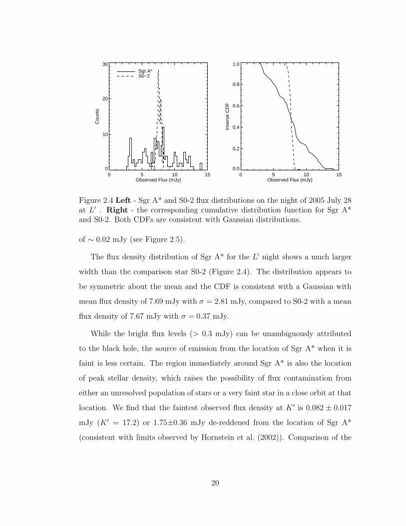
Figure 2.4 Left - Sgr A* and S0-2 flux distributions on the night of 2005 July 28at L′ . Right - the corresponding cumulative distribution function for Sgr A*and S0-2. Both CDFs are consistent with Gaussian distributions.

of ∼ 0.02 mJy (see Figure 2.5).

The flux density distribution of Sgr A* for the L′ night shows a much larger

width than the comparison star S0-2 (Figure 2.4). The distribution appears to

be symmetric about the mean and the CDF is consistent with a Gaussian with

mean flux density of 7.69 mJy with σ = 2.81 mJy, compared to S0-2 with a mean

flux density of 7.67 mJy with σ = 0.37 mJy.

While the bright flux levels (> 0.3 mJy) can be unambiguously attributed

to the black hole, the source of emission from the location of Sgr A* when it is

faint is less certain. The region immediately around Sgr A* is also the location

of peak stellar density, which raises the possibility of flux contamination from

either an unresolved population of stars or a very faint star in a close orbit at that

location. We find that the faintest observed flux density at K ′ is 0.082 ± 0.017

mJy (K ′ = 17.2) or 1.75±0.36 mJy de-reddened from the location of Sgr A*

(consistent with limits observed by Hornstein et al. (2002)). Comparison of the

20

0.00 0.05 0.10 0.15 0.20 0.25 0.30 0.35Observed Flux (mJy)

0

5

10

15

20

25

30

Num

ber

2006−05−03µSgr A* = 0.200σSgr A* = 0.053

µref = 0.151σref = 0.015


0

5

10

15

20

25

30

Num

ber

2006−06−20µSgr A* = 0.180σSgr A* = 0.050

µref = 0.162σref = 0.011


0

5

10

15

20

25

30

Num

ber

2006−06−21µSgr A* = 0.157σSgr A* = 0.046

µref = 0.164σref = 0.015


0

5

10

15

20

25

30

Num

ber

2006−07−17µSgr A* = 0.121σSgr A* = 0.019

µref = 0.119σref = 0.013


0

5

10

15

20

25

30

Num

ber

2007−05−18µSgr A* = 0.185σSgr A* = 0.023

µref = 0.153σref = 0.016


0

5

10

15

20

25

30

Num

ber

2007−08−12µSgr A* = 0.155σSgr A* = 0.010

µref = 0.185σref = 0.011

Figure 2.5 The flux distribution of Sgr A* (solid) of fluxes less than 0.3 mJyand the reference source, S2-133 (dotted) for each night along with the best fitGaussian. On four of the six K ′ nights, the width of the Sgr A* flux distributionis greater than the reference, while in the remaining two nights, the widths arecomparable. Labels are units of mJy.

21

flux distribution of S2-133 with that of Sgr A* below 0.3 mJy shows that, for

four of the six K ′ nights, Sgr A* has a larger variance than S2-133 (see figure

2.5), indicating that Sgr A* is more variable than expected for a stellar source

even at the faintest levels. On the remaining two nights, the variance of Sgr A*

is similar to that of S2-133. On one of these two nights, 2007 August 12, Sgr A*

was fainter than 0.22 mJy for the entire duration of our observation, which makes

this night ideal for timing analysis of Sgr A* at its faintest flux density levels.

Though the flux distribution looks similar to a star, the structure function and

the periodogram shows a slightly steeper slope than expected for Gaussian noise

and as compared to the stellar stellar comparison sources (see Sections 2.2.2.1

and 2.2.2.2). Furthermore, the K ′−L′ color for 2006 July 17, previously reported

in Hornstein et al. (2007), is constant and significantly redder, even at its faintest

on that night, than from a stellar source. At the faintest fluxes, between 0.10 and

0.15 mJy, the mean K ′−L′ spectral slope, corrected for extinction, of Sgr A* has

an average power law exponent of -0.17±0.32, compared to a slope of −0.6± 0.2

from Hornstein et al. (2007). We estimate that a stellar source, which would

have de-reddened spectral slope of 2, could contribute a maximum of about 35%

of the flux to account for the difference in the spectral slope. This leads us to

conclude that, even when the emission is faint, a large fraction of the flux arising

from the location of Sgr A* is likely non-stellar and can be attributed to physical

processes associated with the black hole.

2.2.2 Light Curves and Timing Analysis

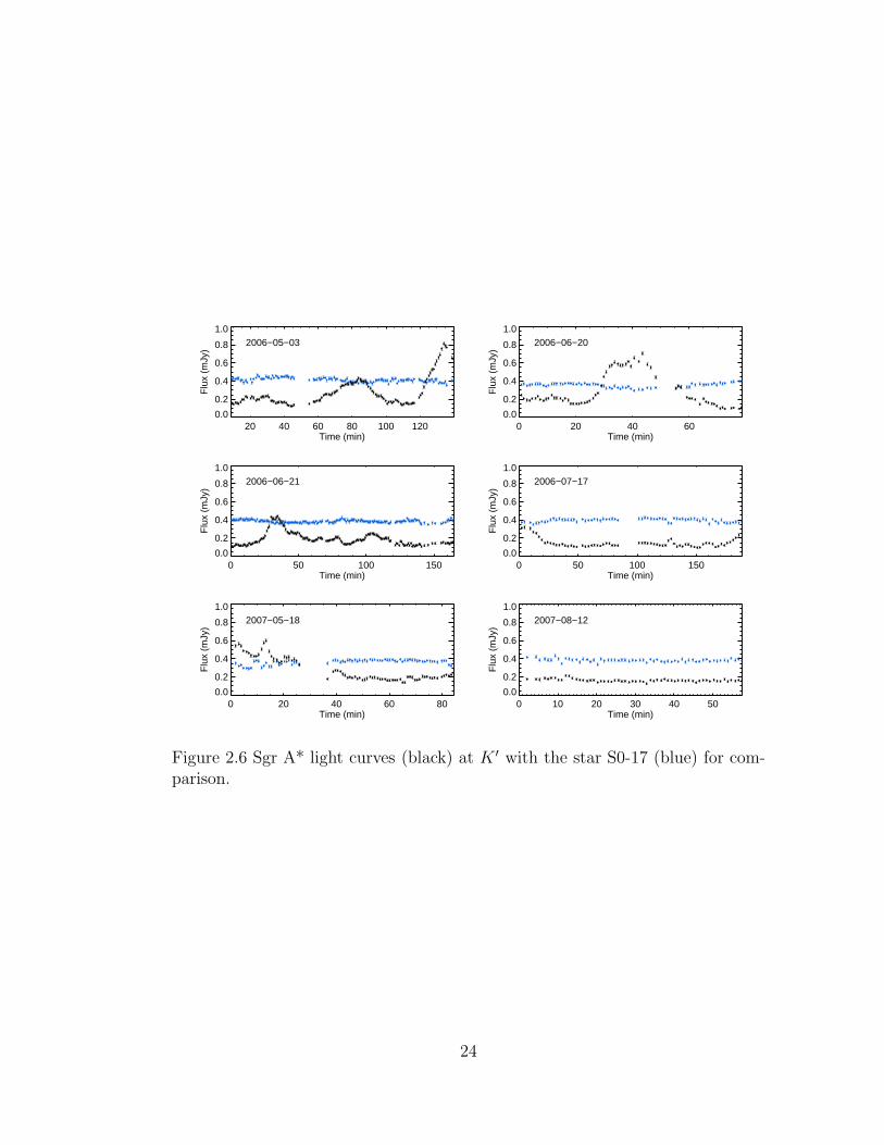
Figures 2.6 and 2.7 shows the resulting light curves for Sgr A* and a non-variable

comparison source for each night of observation. While comparison sources show

no significant time variable emission, Sgr A* shows variations on time scales

22

ranging from minutes to hours, with peak emission that can be 10 times higher

than during its faintest states. The emission peaks are time symmetric, with

similar rise and fall times.

In order to characterize the variability of Sgr A*, we have carried out the fol-

lowing three different approaches to timing analysis: (1) periodograms (2) struc-

ture functions and (3) auto-correlations. The periodogram analysis, presented in

section 2.2.2.1, is effective at pulling out periodic structure in light curves and

therefore is optimal for assessing the presence of any periodicities, such as the

proposed ∼ 20 min QPO reported in previous experiments (e.g., Genzel et al.,

2003a; Eckart et al., 2006b). Both the periodogram and the structure function

can also be used to measure the underlying power spectral density (PSD), which

can then be used to explore similarities to the variability observed in AGNs. We

also compute the auto-correlation for each night to look for possible differences

in the variability at each time scale between each night.

2.2.2.1 Periodogram

It is important to consider all possible sources of noise when testing for period-

icity in light curves. While peaks in the periodograms are a good place to start

searching for periodicity, the peaks must have significantly more power than those

produced by non-periodic processes to be unambiguously attributed to a true pe-

riodicity in any variable source. White (Gaussian) noise processes are unlikely to

lead to large peaks in the periodograms because they contribute equal power at all

frequencies. However, time-correlated physical processes can result in variability

that is frequency dependent. One common variability characteristic - often seen

in AGN light curves - is red noise, which can lead to spurious signals in a power

spectrum or periodogram from a data set having a time baseline only a few times

23

20 40 60 80 100 120Time (min)

0.0

0.2

0.4

0.6

0.8

1.0

Flu

x (m

Jy)

2006−05−03

0 20 40 60Time (min)

0.0

0.2

0.4

0.6

0.8

1.0

Flu

x (m

Jy)

2006−06−20

0 50 100 150Time (min)

0.0

0.2

0.4

0.6

0.8

1.0

Flu

x (m

Jy)

2006−06−21

0 50 100 150Time (min)

0.0

0.2

0.4

0.6

0.8

1.0

Flu

x (m

Jy)

2006−07−17

0 20 40 60 80Time (min)

0.0

0.2

0.4

0.6

0.8

1.0

Flu

x (m

Jy)

2007−05−18

0 10 20 30 40 50Time (min)

0.0

0.2

0.4

0.6

0.8

1.0

Flu

x (m

Jy)

2007−08−12

Figure 2.6 Sgr A* light curves (black) at K ′ with the star S0-17 (blue) for com-parison.

24

0 50 100 150Time (minutes)

0

1

2

3

4

Flu

x (m

Jy)

0.001Frequency (Hz)

0.001

0.010

0.100

1.000

10.000

100.000

Pow

er

Sgr A*Red Noise α = 2.5

3 σ threshold

Figure 2.7 Top: The light curve of Sgr A* (black) and comparison source S0-2(grey) at L′ on 2005 July 28. Bottom: Normalized Lomb-Scargle periodogramsof Sgr A* on this night (black). Also plotted is the 3 σ significance thresholddetermined from Monte Carlo simulations of red noise with a power law index,α = 2.5 (dotted). The average of 105 periodograms with α = 2.5 at the sametime sampling is also shown for comparison (dashed line).

25

longer than that of the putative period, since it will show large amplitude fluctu-

ations at low frequencies and small amplitudes at high frequencies. This can lead

to relatively large stochastic peaks in the power spectrum at low frequencies, far

above what would be expected from white noise. We emphasize that, although

the term for this type of power law dependence of the flux variability is ‘red

noise’, this variability arises from physical processes from the source and is not

a result of measurement uncertainties such as Poisson noise, which behaves like

white noise in its power spectrum.

One of the goals in this timing analysis is to test whether a purely red noise

model can explain the variability of Sgr A*. The PSD of a red noise light curve

is a power law, with greater power at lower frequencies: P (f) ≡ f−α, where f is

the frequency and α is the power law index. For example, α = 0 for white noise

and α = 1 for classical flicker noise (Press, 1978). All red noise simulations in this

paper were produced by an algorithm detailed in Timmer & Koenig (1995), which

randomizes both phase and amplitude of an underlying power law spectrum and

then inverse Fourier transforms it into the time domain to create light curves.

Our procedure for producing simulated light curves is as follows: (1) a light

curve is produced from a PSD with a specific power law slope evenly sampled

at half the shortest observed time sampling interval, with a duration at least 10

times as long as the observed light curve (rounded up to the nearest power of

2 for computational efficiency of the fast Fourier transform). This length was

chosen based upon the suggestion by Uttley et al. (2002) to avoid a ’red noise

leak’ where power is distributed from frequencies lower than that sampled by the

observation into observed frequencies. We find aliasing to be a negligible effect,

because the light curves are generated at higher temporal resolution than the

observations. (2) this light curve is then split into 10 non-overlapping segments

to reduce simulation time (Uttley et al., 2002). Each segment is then re-sampled

26

at the exact sampling times used during the specific night that we are simulating.

(3) since the simulation has an arbitrary flux scale, we scale the light curves to

have the same mean flux level and standard deviation as that night. We also

include the effects of measurement noise in the simulations by adding Gaussianly

distributed noise to each simulated data point. We use our measurements of the

photometric error as a function of flux densities (Section 3.2) of non-variable stars

within 0′′.5 of Sgr A* to account for the flux density dependence in the noise for

each simulated data point.

Instead of computing the PSD, which is often used for evenly sampled data,

we searched for periodicity by computing a related function for unevenly sampled

data: the normalized Lomb-Scargle periodogram (Press & Rybicki, 1989); given

a set of data values hi, i = 1, . . . , N at times ti the periodogram is defined as:

PN(ω) ≡ 1

2σ2

{

[∑

j(hj − h) cos ω(tj − τ)]2∑

j cos 2ω(tj − τ)+

[∑

j(hj − h) sin ω(tj − τ)]2∑

j sin 2ω(tj − τ)

}

(2.1)

where ω is the angular search frequency, h and σ2 are the mean and variance of the

data respectively. The constant τ is an offset introduced to keep the periodogram

phase invariant:

tan (2ωτ) =

∑

j sin 2ωtj∑

j cos 2ωtj(2.2)

Since the periodogram is normalized by the variance of the flux, a light curve

consisting of only white noise, or equivalently, red noise with a power law α = 0,

will have an average power of 1 at all frequencies.

The normalized Lomb-Scargle periodogram was computed for each light curve,

oversampled by a factor of 4 times the independent Fourier intervals in order to

increase the sensitivity to periods between the Fourier frequencies (Figures 2.7

27

and 2.8). Assuming that the physical source of the variability is stationary,

we averaged together the periodograms for the five K ′ nights which have dura-

tions longer than 80 minutes (Figure 2.9). The combined periodogram excludes

the 2007 August 12 night because it is less than an hour long, leading to poor

sampling at low frequencies compared to the other nights. We combined the

periodograms by averaging the Lomb-Scargle power at linearly space frequency

bins. The combined periodogram is consistent with red noise, except for the peak

corresponding to the time scale of the three minute dithers. To characterize the

underlying spectrum, we have performed Monte Carlo simulations combining red

noise light curves with the same sampling as the data set. We tested several

different underlying PSD and found that the combined periodogram is consistent

with power law indices between 2.0 and 3.0, with no periodic components. This

model is able to reproduce the slope of the periodogram, the increase in power at

three minutes from dithering, and the flattening of the periodogram at very low

frequencies caused by poor sampling at those frequencies. The 3 min peak in the

periodogram is repoduced very well by the simulations, showing that the simu-

lations are correctly accounting for the effects of sampling. Figure 2.9 shows the

results of Monte Carlo simulations with power law indices 1.5, 2.0, 2.5, and 3.0.

The simulations shows that the resulting periodograms tend to be flatter than

the intrinsic PSD because the limited time sampling at low frequencies results

in poor sensitivity to long time scale variations characteristic of steeper power

laws. Because the periodogram sampling is poor at frequencies below 40 min

we will ignore those frequencies in all subsequent analysis. We find the resulting

periodograms show less variation for intrinsic PSD α > 2, which suggests that we

have a better constraint on the lower limit than on the upper limit of our estimate

for the slope of the PSD. While red noise models with values of α between 2.0 to

3.0 appear to be consistent with the average periodogram, we will use α = 2.5

28

0.1Frequency (1/min)

0.01

0.10

1.00

10.00

100.00

1000.00

Pow

er

2006−05−03 Sgr A*Red Noise α = 2.5

3 σ threshold


0.01

0.10

1.00

10.00

100.00

1000.00

Pow

er

2006−06−20


0.01

0.10

1.00

10.00

100.00

1000.00

Pow

er

2006−06−21


0.01

0.10

1.00

10.00

100.00

1000.00

Pow

er

2006−07−17


0.01

0.10

1.00

10.00

100.00

1000.00

Pow

er

2007−05−18


0.01

0.10

1.00

10.00

100.00

1000.00

Pow

er

2007−08−12

Figure 2.8 Normalized Lomb-Scargle periodograms of the Sgr A* light curves(black) at K ′. Also plotted is the 3 σ significance threshold determined fromMonte Carlo simulations of red noise with a power law index, α = 2.5 (dottedline). The average of 105 periodograms with α = 2.5 at the same time samplingis also shown for comparison (dashed line).

for the simulations in this work to provide a baseline for comparison. More light

curves will be necessary to determine a reliable intrinsic PSD of Sgr A* (if it does

not vary between nights). Where appropriate, we have also run simulations with

a range of α values to investigate its effects on the statistical significance.

Although there is no evidence for QPO activity in the combined periodogram,

we also test the case of a transient QPO phenomenon in each night. We there-

fore used our best fit of α = 2.5 for the power law of the combined periodogram

to test each night for statistically significant deviations from a purely red noise

model. Our criterion for a statistically significant peak in the periodogram is

29

0.001Frequency (Hz)

0.01

0.10

1.00

10.00P

ower

α = 1.5α = 2.0α = 2.5α = 3.0Sgr A*

0.001Frequency (Hz)

2

4

6

8

10

N p

oint

s

Figure 2.9 Top: averaged periodogram from 5 nights of K ′ observations (blackline) with durations greater than 80 min (resulting in the exclusion of 2007 Aug12). Colored lines are the average of 104 Monte Carlo simulations of combiningdata sets with the same sampling, for three different red noise power laws. Thedotted blue line corresponds to the 3 σ threshold of power for red noise withα = 2.5. The large spike at 0.0056 Hz (3 min) is an artifact resulting fromthe regular dithers in the observations. Bottom: plot of the number of pointscontributing to the averaged periodogram at each frequency.

30

that its power must be above the 99.7% (3σ) confidence interval from a Monte

Carlo simulation with 105 realizations of red noise light curves. This method of

establishing the significance of peaks in the periodogram is similar to the one

proposed by Vaughan (2005) for evenly sampled data, but modified here to ac-

count for our unevenly sampled data set by using the Lomb-Scargle periodogram

instead of the Fourier transform. The resulting periodograms are shown in Fig-

ure 2.8. The individual periodograms show peaks at low frequencies, but these

appear to be consistent with red noise, with no peaks having power greater than

the 3σ threshold derived from the Monte Carlo simulations. No significant peaks

were found when we repeated the same procedure for PSD power law indices

between 1.0 and 3.0.

The periodograms of the comparison sources are much flatter than that of Sgr

A*, as expected for white noise sources. However, there is some power at very low

frequencies (< 40 min), which may be the result of some small time correlated

systematic in the observation such as variations in seeing or AO performance over

a night. Light curves and periodograms from 2006-06-21 of the three comparison

sources S0-17, S0-38, and S2-133 are shown in figure 2.10. The periodograms of

these sources from the other nights of observations are also comparably flat.

By adding an artificial sinusoidal periodic signal to the red noise simulations,

we can address our sensitivity for detecting QPOs in the presence of red noise.

In order to test this, a periodic sinusoidal signal was added to a simulated light

curve with a red noise PSD slope of 2.5, with an amplitude that is a fraction

of the maximum signal in the underlying red noise light curve. This fractional

amplitude of the periodic signal was increased until the periodogram showed a

peak at that frequency above the previously determined 3σ threshold over 98%

of the time. For example, for the time sampling and duration corresponding to

31

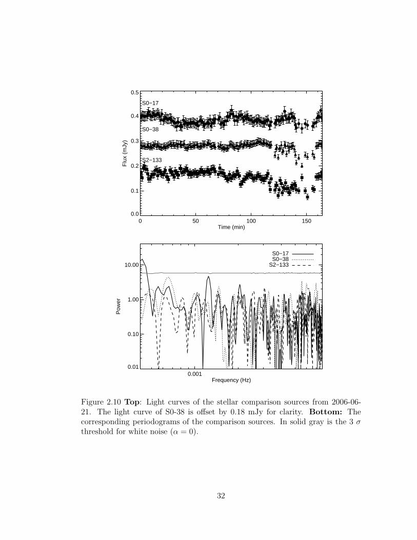
0 50 100 150Time (min)

0.0

0.1

0.2

0.3

0.4

0.5

Flu

x (m

Jy)

S0−17

S0−38

S2−133

0.001Frequency (Hz)

0.01

0.10

1.00

10.00

Pow

er

S0−17S0−38

S2−133

Figure 2.10 Top: Light curves of the stellar comparison sources from 2006-06-21. The light curve of S0-38 is offset by 0.18 mJy for clarity. Bottom: Thecorresponding periodograms of the comparison sources. In solid gray is the 3 σthreshold for white noise (α = 0).

32

20 40 60 80 100 120Time (min)

0.0

0.2

0.4

0.6

0.8

1.0

Flu

x

0.0001 0.0010Frequency (Hz)

0.01

0.10

1.00

10.00

100.00

Pow

er

α = 2.5α = 2.5, 3σ

Figure 2.11 Top: Simulated light curve with the same time sampling as 2006 May03 with a 20 minute periodic signal with an amplitude 15% of the maximum fluxseen that night. Error bars in the light curve are based upon the noise propertiesof that night. Bottom: The corresponding periodogram of the simulated lightcurve (solid line) along with the average (dashed) and 3σ threshold of red noisepower from the Monte Carlo simulations (dotted line). We can recover the signalat 20 min (vertical dotted line) at above our established confidence threshold.

33

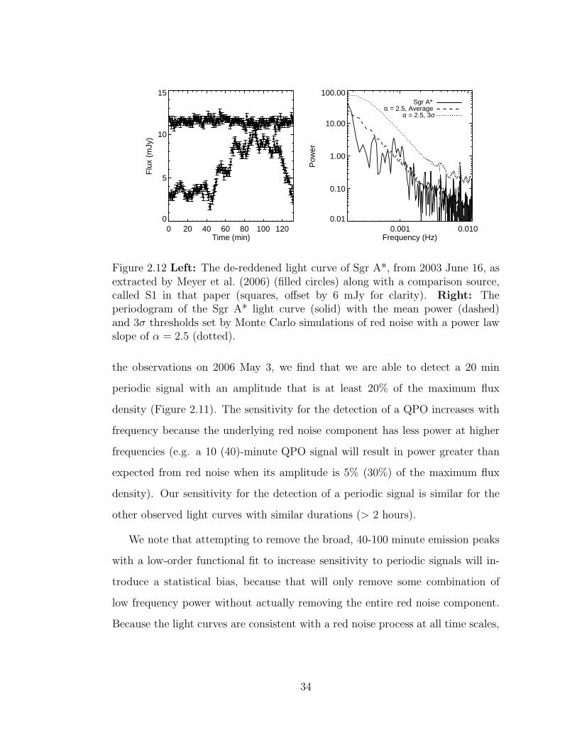
0 20 40 60 80 100 120Time (min)

0

5

10

15

Flu

x (m

Jy)

0.001 0.010Frequency (Hz)

0.01

0.10

1.00

10.00

100.00

Pow

er

Sgr A*α = 2.5, Average

α = 2.5, 3σ

Figure 2.12 Left: The de-reddened light curve of Sgr A*, from 2003 June 16, asextracted by Meyer et al. (2006) (filled circles) along with a comparison source,called S1 in that paper (squares, offset by 6 mJy for clarity). Right: Theperiodogram of the Sgr A* light curve (solid) with the mean power (dashed)and 3σ thresholds set by Monte Carlo simulations of red noise with a power lawslope of α = 2.5 (dotted).

the observations on 2006 May 3, we find that we are able to detect a 20 min

periodic signal with an amplitude that is at least 20% of the maximum flux

density (Figure 2.11). The sensitivity for the detection of a QPO increases with

frequency because the underlying red noise component has less power at higher

frequencies (e.g. a 10 (40)-minute QPO signal will result in power greater than

expected from red noise when its amplitude is 5% (30%) of the maximum flux

density). Our sensitivity for the detection of a periodic signal is similar for the

other observed light curves with similar durations (> 2 hours).

We note that attempting to remove the broad, 40-100 minute emission peaks

with a low-order functional fit to increase sensitivity to periodic signals will in-

troduce a statistical bias, because that will only remove some combination of

low frequency power without actually removing the entire red noise component.

Because the light curves are consistent with a red noise process at all time scales,

34

including the longer broad maxima, any statistical analysis must be performed

without first modifying the light curves. For example, the light curve reported

by Genzel et al. (2003a), the first used to argue for the possible presence of a pe-

riodic variation, shows no significant periodicity when subjected to the red noise

analysis described here. Figure 2.12 shows the analysis of this night using the

light curve re-extracted by Meyer et al. (2006). A significant signal was found

when a low order polynomial fit to the light curve was removed in Meyer et al.

(2006). However, this significance may be biased by the removal of a number of

low frequency components from the light curve.

2.2.2.2 Structure Function

The first order structure function is often used to determine the time scale and

the intrinsic variability in AGN light curves (e.g., Simonetti et al., 1985; Hughes

et al., 1992; Paltani, 1999). Here, we use the structure function to determine the

PSD slope for each night because it is more straightforward to calculate errors in

the structure function. For a set of measurements, s(t) at times t, the first order

structure function V (τ) is defined as:

V (τ) ≡< [s(t + τ) − s(t)]2 > (2.3)

Because this data set is unevenly sampled, we determined the structure function

by calculating [s(t + τ) − s(t)]2 for all possible pairs of time lags and place them

into bins with widths of one fourth of the lag times. Variable bin sizes were

chosen in order to more evenly distribute the number of points in each bin, since

there are many more samples at small lags than at large lags. The median lag

time in each bin is assigned to be the lag time for that bin, while the average of

the V (τ) values in each bin is used as the value of the structure function at that

35

1 10Lag (min)

−4.0

−3.5

−3.0

−2.5

−2.0

−1.5

−1.0

−0.5

Log

Str

uctu

re F

unct

ion

2006−05−032006−06−202006−06−212006−07−172007−05−18

Figure 2.13 The structure functions for five of the K ′ nights for Sgr A* (solid) andthe comparison source, S0-17 (dashed). Error bars are calculated from σ/

√N ,

where σ is the standard deviation and N the number of points in the bin. Errorbars for S0-17 are of comparable sizes, but are omitted for clarity.

lag. The error associated with each bin is σbin/√

Nbin, where σbin is the standard

deviation of the V (τ) values in the bin and Nbin is the number of points. We do

not consider lags with fewer than 5 points in that bin. The resulting structure

functions are presented in Figure 2.13.

Structure functions typically show a power law portion and two plateaus - one

at the time scale of the noise and one plateau at lags longer than the variability

time scale of the underlying physical process. The power law portion of the

structure function is a measurement of the variability of the process. If the

underlying process is stationary, then the logarithmic slope, β (where V (τ) ∝ τβ),

of this region can be related to the power index, α of the PSD (P ∝ f−α). Because

the light curves in this study have finite sampling and duration, this relationship

must be determined separately for each night. To convert the measured structure

function slope into the PSD slope, we measured the slope of an average of 103

36

1 10Lag (minutes)

0.0001

0.0010

Str

uctu

re F

unct

ion

Sgr A*S2−133White Noise

Figure 2.14 The K ′ structure function of Sgr A* (black), S2-133 (blue), andsimulations of white noise (green) for 2007 August 12..

structure functions (β) from simulated light curves for a number of PSD slope

values (α). The relationship between the measured structure function slope and

the PSD slope is linear for values of α between 1.0 and 3.5 (Figure 2.16). These

linear fits are used below to convert between the two slopes. We will use the

structure function to compute the PSD because it is more straightforward than

fitting the periodogram, given the limitations of the time sampling.

The structure function for Sgr A* shows a power law portion at periods greater

than about 1 minute and a flattening at periods greater than about 40 minutes.

This flattening is probably not a sign of a turnover in the intrinsic variability time

scale, but is rather from the poor sampling at longer periods, as shown by large

variations in the value of the structure function from Monte Carlo simulations of

red noise using the same time sampling. This suggests that Sgr A* is likely to be

variable at all the time scales probed in this study. Fits were made to the power

law region of the structure function, typically up to about half or one-third of

37

the total time of observations for each night, and are summarized in Table 2.2.

The best fit power law index for the nights of 2006 May 3 and 2006 June 20,

and 21 has β = 1.4 ± 0.1 (α = 2.7 ± 0.1), between 1 to 20 minutes, consistent

with the fit of α ≈ 2.5 for the slope of the combined periodogram. The other

three nights have slopes ranging from β ≈ 0.8 to β ≈ 0.3. The night with the

flattest slope (2007 August 12) is also the night where the emission from Sgr A*

was faint for the duration of the observation. Figure 2.14 shows that though the

slope, β = 0.26 ± 0.04, is flatter than on other nights, it is significantly steeper

than that of S0-17 (β = 0.04 ± 0.04), S2-133 (β = 0.11 ± 0.05), and simulations

of white noise (β = −0.01), which shows that the emission is not from a constant

background source. The differences in slope between different nights may be

attributable to the increase in photon noise at these faint fluxes (see Section 2.3).

For all nights, the S0-17 structure function is also flat, with a slight rise at longer

time scales (also from poor sampling). The structure function of Sgr A* for the

L′ night on 2005 July 28 has a best fit slope β = 0.77 ± 0.18, corresponding

to α = 1.84 ± 0.27, which is within the range of observed K ′ power law slopes

(Figure 2.15).

2.2.2.3 Auto-correlation

To compare the Sgr A* variability between each night, we computed the auto-

correlation function for each observation. The auto-correlation is defined as:

AC(τ) ≡< [s(t + τ)s(t)] > (2.4)

where s(t) is the measured flux at time, t, and τ is the time lag. Because the light

curves are unevenly sampled, we computed the auto-correlation at all possible

lags and then placed the pairs in bins, similar to our method for the computing

38

Table 2.2. PSD fits from the structure function

Date Fit Range βa αb

(UT) (min)

2006 May 03 1-20 1.37 ± 0.09 2.74 ± 0.132006 June 20 1-20 1.40 ± 0.08 2.79 ± 0.122006 June 21 1-15 1.42 ± 0.18 2.79 ± 0.272006 July 17 1-40 0.71 ± 0.09 1.80 ± 0.162007 May 18 1-20 0.79 ± 0.11 1.95 ± 0.20

2007 August 12 1-30 0.26 ± 0.04 1.06 ± 0.08

aSlope of the power law portion of the structure func-tion, V (τ) ∝ τβ

bSlope of the PSD, P (f) ∝ f−α

10Lag (minutes)

0.001

0.010

0.100

1.000

10.000

Str

uctu

re F

unct

ion

Sgr A*S0−2

Figure 2.15 The structure function of Sgr A* (black), S0-2 (blue) at L′ on 2005July 28. The best fit power law between 3 to 40 min is also plotted. The best fitpower law for Sgr A* is β = 0.77 ± 0.18, corresponding to α = 1.84 ± 0.27 (seeSection 2.2.2.2 for details).

39

0.0 0.5 1.0 1.5Measured SF Index, β

0.0

0.5

1.0

1.5

2.0

2.5

3.0

PS

D In

dex,

α

2006−05−032006−06−202006−06−212006−07−172007−05−182007−08−12

Figure 2.16 The relationship between intrinsic PSD power index and the measuredpower law of the structure function as simulated for the time sampling on eachnight. The line fits are made for PSD power law slope α > 1.0 in the linearregion of the relationship between the intrinsic PSD power law and the structurefunction power law.

of the structure function. We find that the correlation coefficients at time scales

up to 40 minutes are consistent across all nights. At time lags greater than 40

minutes, the auto-correlations appear to diverge from each other. This is mostly

likely from poor sampling at those frequencies. From Monte Carlo simulations of

red noise with the same time sampling as the data set, we find that the lags greater

than about 40 minutes have large variations in auto-correlations coefficients; we

therefore defer interpretations of lags greater than 40 minutes until more data is

available to better sample these time scales.

2.3 Discussion

Our analysis shows that the Sgr A* near-infrared light curves observed in this

study are entirely consistent with red noise with no significance evidence for a

40

QPO signal near 20 min (or any other time scale). In addition, power is seen at the

shortest time scales measured in the periodogram (2 min), well below the orbital

period at the last stable circular orbit of a spinning black hole (∼ 5–30 min).

This indicates that the high frequency variability is not simply from Keplerian

motion of a single orbiting ‘hot spot’ producing the near-IR flux modulations

(Meyer et al., 2006; Trippe et al., 2007). The high frequency variability must

originate from small areas of the accretion flow. In addition to power at high

frequencies, the light curve for 2007 May 18 shows a strong spike in flux at about

10 min with a duration of ∼ 5 min, and a rise time of only ∼ 3 min, which also

suggests that regions of the accretion flow responsible for the variability can be

as small as 0.4 AU.

It is important to note that the significance threshold used in this study tests

whether the periodogram power of peaks exceeds 3σ at a given frequency. It

does not take into account that we are scanning over a large range of frequencies.

If one searches enough frequencies, a peak of arbitrary power will appear at a

random frequency. If a peak in the periodogram was found in this study that

may indicate a periodic signal, then additional simulations should be performed

to determine its statistical significance by accounting for the range of frequencies

probed. This is referred to as the false alarm probability in Horne & Baliunas

(1986) and has been calculated analytically for the case of white noise. In the case

of red noise, the additional simulations would also need to account for the fact

that larger peaks are more likely at low frequencies (Meyer et al., 2008, 2009).

2.3.1 Comparisons with X-ray variability

The timing analysis of Sgr A* in the infrared may be a way to compare the

signatures of physical processes operating in the accretion flow of Sgr A* to

41

those of AGNs. Because AGN variability studies are usually performed on X-

ray observations, the ideal comparison of the variability of Sgr A* to that of

AGNs should be done at X-ray energies. However, X-ray emission from the

inner accretion flow of Sgr A* can only be currently detected above the diffuse

background during large flaring events. Simultaneous multi-wavelength studies of

Sgr A* have shown that every detectable X-ray flare shows corresponding peaks

in the near-IR, with no apparent time lag (Yusef-Zadeh et al., 2006; Eckart et al.,

2006a). The spectral slope is also similar at X-ray and infrared wavelengths

(Sν ∝ ν−0.6: Belanger et al., 2005; Yusef-Zadeh et al., 2006; Hornstein et al.,

2007), which supports a model in which the X-ray photons are the result of

synchrotron self Compton scattering of lower energy photons from the population

of electrons that produce synchrotron emission seen in the infrared. If the infrared

and the X-ray emissions are produced by the same population of electrons, then

our infrared measurements can be used as a proxy for the X-ray variability; we

find that the periodograms of the infrared light curves of Sgr A* are in fact

consistent with having intrinsic PSD slopes similar to those reported for AGNs

at X-ray wavelengths (α ≈ 1 − 3) (e.g. Lawrence & Papadakis, 1993; Kataoka

et al., 2001; Markowitz et al., 2003). Our observations are consistent with Sgr

A* being variable at all time scales between ∼ 2 minutes to ∼ 1 hour with no

changes in PSD slope between these time scales during the observations period on

any single night. This steeply rising power law cannot be extended to arbitrarily

low frequencies because the integrated power would diverge. For example, AGNs

typically show either one or two breaks in their power spectrum, with recent

evidence suggesting that these breaks scale with the mass and accretion rate of

the AGN (McHardy et al., 2006). The lack of a break in the Sgr A* periodogram

is not unusual because the breaks seen in AGNs are at time scales on the order

of days or weeks (Markowitz et al., 2003). Using the relationship between the

42

break frequency, the black hole mass, and accretion rate found by McHardy et al.

(2006) for stellar mass black holes and AGNs, the predict break frequency for

Sgr A* is ∼ 1 × 106 days. However, a direct comparison to AGNs is difficult

at this time because the physical scales involved are so different; the cores of

AGNs in which variability is usually measured have sizes on the order of parsecs,

whereas Sgr A* is unresolved in this study at a resolution of 65 mas, or ∼ 540

AU. The accretion luminosities of AGNs with well measured timing properties

are substantial fractions of their Eddington luminosity compared to the 10−9

Eddington luminosity for Sgr A*, which may make the comparison inapplicable

as well. Nevertheless, the variability properties of Sgr A* are valuable additions

to the broadband spectrum since any models that can produce the observed

spectrum should also be able to account for the timing characteristics.

2.3.2 The effect of measurement noise on the inferred PSD slope

While it may appear from the results in Section 2.2.2.2 that the slope of the

power spectrum is changing between nights, the red noise simulations show that,

as the amplitude of the red noise signal decreases, photon noise will increasingly

dominate the measurement of the slope, thus biasing the measurement of the

true slope of the underlying red noise process. To determine when photon noise

becomes important to the slope measurements, we performed Monte Carlo sim-

ulations of light curves with time sampling from 2008 August 12 and assuming

an intrinsic α = 2.5 for various values of the ratio of the standard deviation of

the red noise signal to the standard deviation of the expected measurement noise

(σred noise/σwhite noise). Average values of α were extracted from 200 simulated

light curves at each value of σred noise/σwhite noise from 0.1 - 100.0 (Figure 2.17).

We find that as σred noise/σwhite noise becomes smaller, the measured value of α

43

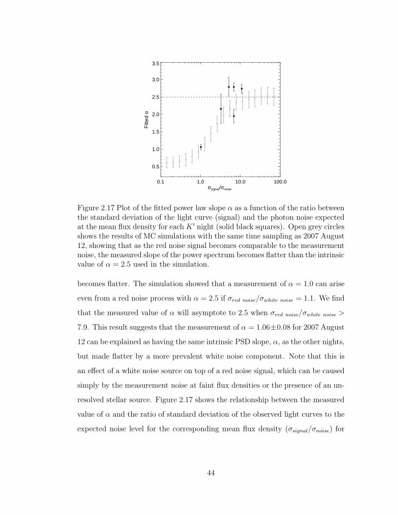
0.1 1.0 10.0 100.0σsignal/σnoise

0.5

1.0

1.5

2.0

2.5

3.0

3.5

Fitt

ed α

Figure 2.17 Plot of the fitted power law slope α as a function of the ratio betweenthe standard deviation of the light curve (signal) and the photon noise expectedat the mean flux density for each K ′ night (solid black squares). Open grey circlesshows the results of MC simulations with the same time sampling as 2007 August12, showing that as the red noise signal becomes comparable to the measurementnoise, the measured slope of the power spectrum becomes flatter than the intrinsicvalue of α = 2.5 used in the simulation.

becomes flatter. The simulation showed that a measurement of α = 1.0 can arise

even from a red noise process with α = 2.5 if σred noise/σwhite noise = 1.1. We find

that the measured value of α will asymptote to 2.5 when σred noise/σwhite noise >

7.9. This result suggests that the measurement of α = 1.06±0.08 for 2007 August

12 can be explained as having the same intrinsic PSD slope, α, as the other nights,

but made flatter by a more prevalent white noise component. Note that this is

an effect of a white noise source on top of a red noise signal, which can be caused

simply by the measurement noise at faint flux densities or the presence of an un-

resolved stellar source. Figure 2.17 shows the relationship between the measured

value of α and the ratio of standard deviation of the observed light curves to the

expected noise level for the corresponding mean flux density (σsignal/σnoise) for

44

all K ′ nights. The measured value of α appears to asymptote on nights when the

red noise amplitude is stronger. This relationship is consistent with that found in

the Monte Carlo simulations, where the nights with lower values of σsignal/σnoise

have flatter red noise spectra than those on the nights with greater fractional

signal variance. These results show that the differences between the measured

slopes for different nights may be explained by the effect of measurement noise

on light curves with faint fluxes.

We also considered how a slightly time correlated source would affect the

power law slope measurements by including a time correlated source with a small

α into the simulations and varying its signal strength as the above treatment

with white noise. This is motivated by the fact that there is a slight slope

to the structure function of our comparison source S2-133. For example on 12

August 2007, S2-133 has a structure function power law slope of β = 0.11± 0.05

corresponding to α = 0.7 ± 0.2. We find that the addition of such a background

source increases the measured Sgr A* PSD power law slope α by a maximum of

0.1, which is about the same level as our fitting error. The effect of a slightly time

correlated background source thus appears to be a source of systematic error, but

one which does not significantly affect our results.

2.3.3 Limits on a quiescent state of Sgr A*

A notable feature of the light curves in these observations is that there appears

to be a lower limit, or ‘floor’ to the light curves from each night. This lower

limit is not an observational constraint, because we are able to reliably detect

stars within 0′′.5 of Sgr A* to K′ ≈ 19 mag compared to the faintest Sgr A*

observation at K ′ ≈ 17 mag. A question to be investigated in future studies

is whether this represents a ‘quiescent’ state of Sgr A*, characterized by lower

45

variability at that flux level or is a faint star confused with Sgr A*. If the low flux

density state is a physically distinct state, then the large flux variations would

be the result of additional emission of energy above this quasi-steady state. To

examine the nature of this faint state, we can look to the peak of the distribution

of flux densities fainter than ∼ 0.3 mJy for each night. We find that the flux

density of the peak of this distribution shifts slightly between different nights of

observations. However, this shift appears only to be marginally significant given

the lower photometric accuracy at the fainter flux levels. Before physical models

can be applied to the faint state, a more detailed analysis of the light curves is

necessary to establish whether this state exists. If the faint state of Sgr A* can

be modeled as arising from the steady accretion of mass, then the slight drift of

this mean flux level may be explained by a gradual change in the accretion rate.

Another explanation for the drift in the mean Sgr A* flux density is that it is

due to very long timescale flux variation from the red noise power law behavior

of the flux as in AGNs.

It is clear that Sgr A* can now always be detected in the infrared using LGS

AO and that even at low flux densities, the K ′−L′ color of the source appears to

be redder and have PSD slopes steeper than a star, but the measurement errors

do not rule out the possibility of a faint stellar component in the near-infrared flux

from the location of Sgr A*. More observations during both the faint and bright

states of Sgr A* are necessary to confirm whether there truly exists a quiescent

state with different timing behavior. Since Sgr A* is much redder than any stellar

source, observations at L′ would be much less affected by stellar contamination

than at K ′, thus the test for a quiescent state may be more conclusive at L′.

Note that the existence of a quiescent state does not affect the timing analysis

for periodic signals because the mean flux density is subtracted from a light curve

to remove the zero frequency power before creating the periodogram.

46

While no QPO signal was detected in this study, this does not preclude the

possibility for a transient periodic signal in other observations. In addition, a

periodic signal with an amplitude below our detection threshold would also be

difficult to detect unless the signal is consistently at the same frequency such

that it would become statistically significant in a combined periodogram. More

observations of Sgr A* would be helpful to investigate such low amplitude QPO

signals.

2.4 Conclusion

We have obtained 7 near-infrared light curves of Sgr A* using NGS and LGS AO

and through Monte Carlo simulations, test for a periodic signal in the presence of

red noise with unevenly sampled data. We find no statistically significant QPO

signals in any of the Sgr A* light curves observed in this study; the variability

appears to be consistent with a physical process having a power spectrum index

α ∼ 2.5 in the averaged periodogram, with variations between α = 1.0 to 2.8

between different nights. A determination of the true PSD power law slope of

Sgr A* will require at least double the number of light curves observed in this

study so that more sophisticated spectral estimation techniques can be used (e.g.

Priestley, 1981; Papadakis & Lawrence, 1993). While more data will be necessary

to reliably determine the intrinsic PSD slope, it is unnecessary to invoke a periodic

signal to describe the variability of the light curves observed in this study. We

have also shown the importance of preforming statistical tests for QPO signals

using the entire Sgr A* light curve. Removing broad large amplitude peaks

eliminates some combination of low frequency power, artificially boosting the

significance of mid-range frequencies without actually removing the underlying

red noise component.

47

The mechanism producing the infrared variability in Sgr A* in these obser-

vations may be related to the processes occurring in AGNs or accreting black

hole binaries, based on the similarity of their timing properties. Detailed model

comparison between Sgr A* and other accreting black hole systems will require

continuous observations over longer time scales and at faster time sampling to

detect possible low and high frequency breaks, respectively, in the power spec-

trum.

48

CHAPTER 3

High angular resolution integral-field

spectroscopy of the Galaxy’s nuclear cluster: a

missing stellar cusp?

3.1 Introduction

Over 30 years ago, theoretical work suggested that the steady state distribution

of stars may be significantly different for clusters with a massive black hole at

the center than those without (e.g. Bahcall & Wolf, 1976; Cohn & Kulsrud, 1978;

Young, 1980). Stars with orbits that bring them within the tidal radius of the

black hole are destroyed and their energy is transferred to the stellar cluster. In

the steady state, this energy input must be balanced by the contraction of the

cluster core, which appears as a steeply rising radial profile in the number density

of stars toward the cluster center. This radial profile is usually characterized by

a power law of the form n(r) ∝ r−γ, with a power law slope, γ, that is steeper

than that of a flat isothermal core. For a single-mass stellar cluster, Bahcall &

Wolf (1976) determined the dynamically relaxed cusp will have γ = 7/4. The

presence of such a steep core profile, or cusp, is important observationally because

it may represent a simple test for black holes in stellar systems where dynamical

mass estimates are difficult, such as in the cores of galaxies. The stellar cusp

is also important theoretically as it is a probable source of fuel for the growth

49

of supermassive black holes and its presence is often assumed in simulations of

stellar clusters having a central black hole (e.g., Merritt, 2005, and references

therein).

Theoretical work has progressed from the early simulations by Bahcall & Wolf

(1976) to include many complicating effects, including multiple masses, mass

segregation, and stellar collisions, on the density profile of stellar clusters in the

presence of a supermassive black hole (e.g., Bahcall & Wolf, 1977; Murphy et al.,

1991; Alexander & Hopman, 2008). These theories predict cusp slopes within a

black hole’s gravitational sphere of influence ranging from 7/4 ≥ γ ≥ 7/3 for a

multiple mass population to as shallow as γ = 1/2 for a collisionally dominated

cluster core. An important assumption of all cusp formation models is that

the stellar cluster be dynamically relaxed. Without this assumption, the stellar

distribution would show traces of the cluster origin in addition to the influence

of the black hole.

The Galactic center is an ideal place to test these theories of cusp formation as

it contains the nearest example of a supermassive black hole (Sgr A*, with a mass

M• = 4.1± 0.6× 106 M⊙, Ghez et al., 2008; Gillessen et al., 2009). Located at a

distance of only 8 kpc, the radius of the sphere of influence of the Galactic center

black hole (∼ 1 pc) has an angular scale of ∼ 25′′ in the plane of the sky, two

orders of magnitude larger than any other supermassive black hole. In order to

plausibly test stellar cusp formation theories, the stellar population used to trace

the cusp profile must be older than the relaxation time, which is of order 1 Gyr

within the sphere of influence of Sgr A* (e.g., Hopman & Alexander, 2006). In

the Galactic center, late-type red giants (K to M) are the most promising tracers

of the stellar distribution since they are > 1 Gyr old, bright in the NIR, and

abundant. On parsec size scales, these stars dominate the flux, so early seeing

50

limited observations of the surface brightness profile in the NIR at the Galactic

center were successfully used to show that the structure of the nuclear star cluster

at large scales has a density power law of γ ≈ 2 (Becklin & Neugebauer, 1968).

Integrated light spectroscopy of the CO absorption band-head at 2.4 µm (which is

dominated by red giants) also confirmed this slope down to within ∼ 0.5 pc from

the black hole (McGinn et al., 1989; Haller et al., 1996). These measurements,

as well as integrated light spectroscopy from Figer et al. (2000) of the inner 0′′.3,

found a lack of CO absorption in the inner ∼ 0.5 pc of the Galaxy. It was

unclear at the time whether this represented a change in the stellar population

with fewer late-type stars in the inner region or a change in the stellar density

profile. Because the integrated light spectrum is biased toward the brightest stars,

contamination from a few young Wolf-Rayet (WR) stars (age < 6 Myr), such as

the IRS 16 sources identified in the early 1990s located between 1–2′′ from the

black hole (e.g., Allen et al., 1990; Krabbe et al., 1991), can significantly impact

measurements of the underlying stellar density.

Several approaches have been taken to identify the cause of the difference in

the CO equivalent width in the integrated light within the inner 0.5 pc of the

Galaxy. Scoville et al. (2003) attempted to remove the effects of the bright young

stars on the surface brightness distribution through narrow band imaging with

NICMOS/HST. They found a surface brightness that began to flatten and drop

slightly in the central 0.1 pc. Since fainter young stars can still contribute to

the surface brightness, Genzel et al. (2003b) used adaptive optics (AO) imaging

with H (1.6 µm) and Ks (2 µm) filters to measure the stellar density using

number counts, which they argue more robustly traced the population of red

giants. They find γ = 2.0 ± 0.1 at R ≥ 10′′ and γ = 1.4 ± 0.1 at R < 10′′,

which suggests that there may be a stellar cusp at the Galactic center within

the range predicted by Bahcall & Wolf (1977). Further work by Schodel et al.

51

(2007), which included deeper AO imaging, produced a fit of a broken power law

to the observed projected surface number density profile of the form Σ(R) ∝ R−Γ,

where R is the projected distance from Sgr A* in the plane of the sky, and Γ the

projected power law slope. Their best fit broken power law model has a break

radius at Rbreak = 6′′.0 ± 1′′.0 (0.22 pc), with Γ = 0.75 ± 0.1 outside Rbreak and

Γ = 0.19 ± 0.05 as the slope of the stellar cusp inside Rbreak. This indicated

that the cusp slope is perhaps flatter than the range predicted by Bahcall & Wolf

(1977). However, with only number counts, it was still unclear how much bias to

the slope was contributed by the dynamically unrelaxed young stellar population,

which represents a large fraction of the bright stars (K ′ < 14) that have been

spectroscopically identified in the inner 1′′ (e.g., Ghez et al., 2003; Paumard

et al., 2006).

To make further progress, it is necessary to discriminate between the early

and late-type stars. One recent approach has been through narrow-band imaging

to target wavelengths where there are measurable differences between spectral

features of the two types of stars. For example, the CO bandhead absorption

features starting at 2.29 µm are very strong for late-type stars (K & M), and

absent for early-type stars (O & early B). Using the CO narrowband images

from the Gemini North Galactic Center Demonstration Science Data Set, Genzel

et al. (2003b) found that the fraction of late-type stars declines between 10′′

and 1′′ from the Galactic center, and thus, may be flatter than expected from

number counts. However, this narrowband dataset was shallower than that of

the broadband images used in the number counts measurements and had trouble

differentiating between the two types of stars at K > 13. More recently, Buchholz

et al. (2009) took deeper narrowband images (K < 15.5) in CO and found an

even more shallow slope in the inner region of the cluster. Their best fit slope of

Γ = −0.17±0.09 at R < 6′′.0 suggests that the late-type stars may even be slightly

52

declining toward the cluster center. While number counting with narrowband

images has greater discriminating power than broadband images, this method has

limitations. First, this method is strongly dependent on how well the dataset can

be calibrated based upon existing spectroscopically determined samples, which

is limited to K< 13. In addition, limits on the CO equivalent widths depend on

how precisely the slope of the stellar continuum can be measured with narrow

band filters.

A spectroscopically selected sample would be ideal to separate the late-type,

presumably dynamically relaxed population from that of the young early-type

stars. Until recently, much of the spectroscopy taken of stars in the Galactic

center has been seeing-limited and limited in sensitivity to K < 13 (see Genzel

et al., 2000; Blum et al., 2003; Figer et al., 2003). These surveys found a drop in

the fraction of late-type stars toward the central ∼ 10′′, but because they were

sensitive only to the brightest giants, the uncertainty remained as to whether the

fainter stars would show the same trend. Nevertheless, these results combined

with measurements from imaging all point toward fewer stars in the central 0.5

pc than would be expected for a relaxed cusp.

By combining the advantages of high spatial resolution from AO imaging with

the discriminating power of spectroscopy, the advent of integral-field spectroscopy

(IFU) behind AO has potential to provide the most sensitive method of measuring

the stellar cusp profile in the inner 0.5 pc of the Galaxy. Measurements with the

SINFONI IFU at the VLT have shown that it is possible to identify young stars

at better than 100 mas angular resolution (Paumard et al., 2006; Gillessen et al.,

2009). Here, we report on a high angular resolution spectroscopic survey of the

central 0.15 parsec of the Galaxy using laser guide star adaptive optics with the

OSIRIS IFU at the Keck II telescope. The survey reaches a completeness of 40%

53

at K ′ ≈ 15.5, two magnitudes fainter than previously reported spectroscopic

surveys of late-type stars in this region. The observations and data reduction

method are described in Section 3.2 and 3.3. Using these observations, it is

possible to separate the presumably dynamically relaxed late-type population

from the young, unrelaxed population (Section 3.4). We find that the surface

number density of late-type stars is significantly flatter than the range of power

laws predicted by Bahcall & Wolf (1977) (Section 3.5). This measurement rules

out all values of γ > 1.0 at a confidence level of 99.7%. In Section 3.6, we

discuss possible dynamical effects that may lead to the flat observed slope and

implications for future measurements of the stellar cusp at the Galactic center.

3.2 Observations

Near-IR spectra of the central 4′′ of the Galaxy were obtained between 2006

and 2009 using the OSIRIS integral field spectrograph (Larkin et al., 2006) in

conjunction with the laser guide star adaptive optics (LGS AO) system on the

Keck II telescope (Wizinowich et al., 2006; van Dam et al., 2006). The laser guide

star was propagated at the center of our field and for low-order tip-tilt corrections,

we used the R = 13.7 mag star, USNO 0600-28577051, which is located ∼ 19′′

from Sgr A*. The AO system enabled us to obtain nearly diffraction limited

spatial resolution (∼ 70 mas) in our long-exposure (15 min) 2 µm data sets. All

observations were taken with the narrow band filter Kn3 (2.121 to 2.229 µm)

centered on the Br γ hydrogen line at 2.1661 µm, with a pixel scale of 35 mas

and a spectral resolution of ∼ 3000. With this filter, OSIRIS has a field of view of

1.′′68×2.′′24 per pointing and offers sensitivity to both early and late-type stars.

Early-type stars from OB supergiants to B type main sequence young stars show

a prominent Br γ line, while late-type (K & M) evolved giants contain strong Na

54

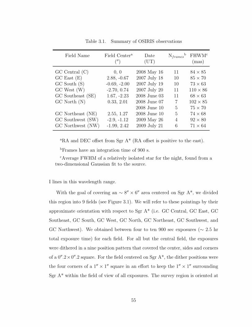
Table 3.1. Summary of OSIRIS observations

Field Name Field Centera Date Nframesb FHWMc

(′′) (UT) (mas)

GC Central (C) 0, 0 2008 May 16 11 84 × 85GC East (E) 2.88, -0.67 2007 July 18 10 85 × 70GC South (S) -0.69, -2.00 2007 July 19 10 73 × 63GC West (W) -2.70, 0.74 2007 July 20 11 110 × 86GC Southeast (SE) 1.67, -2.23 2008 June 03 11 68 × 63GC North (N) 0.33, 2.01 2008 June 07 7 102 × 85

2008 June 10 5 75 × 70GC Northeast (NE) 2.55, 1.27 2008 June 10 5 74 × 68GC Southwest (SW) -2.9, -1.12 2009 May 26 4 92 × 80GC Northwest (NW) -1.99, 2.42 2009 July 21 6 71 × 64

aRA and DEC offset from Sgr A* (RA offset is positive to the east).

bFrames have an integration time of 900 s.

cAverage FWHM of a relatively isolated star for the night, found from atwo-dimensional Gaussian fit to the source.

I lines in this wavelength range.

With the goal of covering an ∼ 8′′ × 6′′ area centered on Sgr A*, we divided

this region into 9 fields (see Figure 3.1). We will refer to these pointings by their

approximate orientation with respect to Sgr A* (i.e. GC Central, GC East, GC

Southeast, GC South, GC West, GC North, GC Northeast, GC Southwest, and

GC Northwest). We obtained between four to ten 900 sec exposures (∼ 2.5 hr

total exposure time) for each field. For all but the central field, the exposures

were dithered in a nine position pattern that covered the center, sides and corners

of a 0′′.2×0′′.2 square. For the field centered on Sgr A*, the dither positions were

the four corners of a 1′′ × 1′′ square in an effort to keep the 1′′ × 1′′ surrounding

Sgr A* within the field of view of all exposures. The survey region is oriented at

55

4 2 0 −2 −4RA Offset (arcsec)

−4

−2

0

2

4

DE

C O

ffset

(ar

csec

)

N

E

Figure 3.1 The currently surveyed region overlaid on a K′ (2.2 µm) image ofthe Galactic center taken in 2007. Sgr A* is marked at the center with a *.Spectroscopically identified early (blue triangles) and late-type (red circles) starsare marked. Each field is enclosed by dotted lines. Some spectral identificationsare outside of the marked lines because they were found at the edge of the dithers.

a position angle (PA) of ∼ 105 degrees, with the longer direction oriented along

major axis of the disk of young stars rotating in the clockwise direction in the

plane of the sky (Paumard et al., 2006; Lu et al., 2009). Table 3.1 summarizes

these observations.

56

3.3 Data Reduction

Data cubes with two spatial dimensions and one spectral dimension were pro-

duced using the OSIRIS data reduction pipeline provided by Keck Observatory.

The pipeline performs dark current subtraction, cosmic ray removal, and wave-

length rectification. The cubes were not corrected for the effects of chromatic

differential atmospheric dispersion because this effect is small within the wave-

length range of Kn3, shifting the centroid of stars by only 0.1 spatial pixel between

the shortest and longest wavelength channel.

For each field, stellar positions were estimated by running StarFinder, a point

spread function (PSF) fitting program (Diolaiti et al., 2000), on images made

from collapsing the data cubes along the spectral dimension. First, a mosaic

was made by combining the individual dithers within each field with the OSIRIS

pipeline using an average for all overlapping spatial pixels. An image was then

created from the mosaicked cube by taking the median of the spectral channels

at each spatial pixel. Next, between 1–3 of the brightest, most isolated stars were

chosen by hand as PSF reference stars for StarFinder. This PSF was then used to

determine the centroids of all the stars in the mosaic in an initial pass. After the

first attempt at identifying sources, we ran an additional iteration of StarFinder

to improve the estimate of the PSF, which is then used in a second pass to deter-

mine centroids. The stars identified by this process were cross-checked with the

nearest epoch of deep images taken at K ′ using LGS AO with the NIRC2 imager

on Keck II (Ghez et al., 2008) in order to remove false detections in the noisier

OSIRIS data and to obtain accurate broadband photometric measurements for

these stars. As a final step, StarFinder was run on each individual cube using rel-

ative positional priors from the deeper mosaic cubes and the PSF as determined

from the OSIRIS mosaic to obtain precise OSIRIS positions in preparation for

57

spectral extraction from the individual data cubes.

The spectrum of every star was then extracted from each cube by performing

aperture photometry for the star at each spectral channel. We used an aperture

of radius 2 pixels (70 mas) to extract the stellar spectrum and the median of an

annulus with inner radius at 2 pixels and outer radius at 4 pixels to determine

the sky background. For regions with very high stellar density, such as within

the central arcsecond, the background was manually determined by the median

of patches of sky free of stars as close to the target star as possible. The final

spectrum of each star was then produced by averaging the spectra of that star

from all data cubes from that night. When the signal to noise ratio (SNR)

per spectral channel between the spectra were significantly different, they were

combined using an average weighted by the SNR (calculated between 2.212 to

2.218 µm).

The combined spectra have SNRs ranging from over 100 for bright stars (K′ <

13) to ∼ 5 for the faint stars (K′ ≈ 15.5) that have marginal line detections.

Photon noise appears to dominate the SNR of the final spectra and thus our

ability to assign spectral types to most of the stars. In addition, regions with

strong gas emission such as along the mini-spiral (Paumard et al., 2004) and

within the central arcsecond can be problematic for identifying Br γ absorption

lines from early-type stars. Interstellar Br γ emission can be quite strong and

can have several kinematic components, which can lead to a systematic bias in

the measurement of the Br γ line in the early type stars if the background gas

component is not completely corrected. Confusion is also a problem around very

bright sources such as the IRS 16 stars, where we were unable to extract several

K ′ ≈ 13 stars that were identified in NIRC2 images1.

1NIRC2 is less sensitive to confusion because the plate scale is 10 mas compared to 35 masused in the OSIRIS observations and the higher strehl ratios obtained from the much shorter

58

An A0V (HD 195500) and G2V (HD 193193) star were observed on each night

to correct for atmospheric absorption lines2. The A star, having no intrinsic

absorption lines other than Br γ and He I in the Kn3 filter, serves as a good

indicator of atmospheric and instrumental features. To remove the Br γ and

He I line from the A0V spectrum, we replace the region between 2.155 to 2.175

µm with the same region from the G2V star and divided by the empirically

observed solar spectrum shifted to the radial velocity of the G2V star (similar to

the procedure described in Hanson et al. (1996)). The A star spectrum was then

divided by a 10,000 K blackbody to remove the stellar continuum.

3.4 Spectral Identification

Given our survey sensitivity, we expect to be able to detect the early-type stars

in the form of bright Wolf-Rayet stars, OB supergiants, main sequence young

stars down to B2-B4V, and late-type stars in the form of K-MIII evolved giants.

The most important feature of this survey is its ability to differentiate between

early and late-type stars. This distinction is apparent when comparing template

spectra of early type stars with those of late type giants, even in the limited Kn3

wavelength range; the young stars have featureless spectra except for Br γ and

He I at 2.1661 and 2.1641 µm, respectively, while the late-type stars lack these

high temperature lines and show a plethora of other atomic and molecular lines,

most prominently the Na I lines at 2.2062 and 2.2090 µm.

In order to assign spectral types to the stars, we separate all the extracted

spectra by visual inspection into five groups: 1. Spectra with prominent Br γ

lines and no Na I lines are identified as early-type stars (e.g., S0-2 in Figure 3.2).

exposures (30 s vs. 900 s)2These stars were observed using natural guide star mode with 30 s integration time and 5

frames per star.

59

2.14 2.16 2.18 2.20 2.22Wavelength (µm)

0.0

0.2

0.4

0.6

0.8

1.0

1.2

Flu

x

S0−2, Early−type

S2−74, Early−type

S0−13, Late−type

Br

γ

Na

IN

a I

Figure 3.2 Example of observed spectra in the Kn3 narrowband wavelength regionof early and late-type stars. The Br γ and Na I lines are used to differentiatebetween early and late-type stars, respectively. S0-2 is a K ′ = 14.1 early-type starwith a strong Br γ line. S2-74 is a K ′ = 13.3 early-type star showing a featurelessspectrum in the OSIRIS Kn3 filter wavelength range. S0-13 is a K ′ = 13.5 late-type star showing the Na I doublet. See Figures 2a, 2b, and 2c in Appendix ??

for the spectra of all stars with spectral identification.

60

2. Spectra with prominent Na I lines, but no Br γ line are identified as late-type

stars (e.g., S0-13 in Figure 3.2). 3. Low SNR (< 5) spectra with no apparent

lines are classified as unknown. 4. Bright stars with high SNR (K′ < 14, SNR

> 40) spectra with no late-type or Br γ lines are identified as young. These

are most likely late O-type stars, which have very small or undetectable Br γ

absorption lines at the resolution of this survey (Hanson et al., 1996) (e.g., S2-74

in Figure 3.2). 5. Spectra with both Br γ and Na I lines are identified as late-type

if there is strong gas emission nearby, which would explain the Br γ line as an

over-subtraction of the background gas (2 stars showed these features). Using

these criteria in the survey region, we classified 68 stars as early-type (24 newly

identified) and 86 stars as late-type (73 newly identified). The late and early-type

stars are reported in Tables 3.2 and 3.3 and labeled in Figure 3.1. The stars with

successfully extracted spectra, but have undetermined spectral types are listed in

Table 3.4. Our ability to classify the stars is strongly dependent on the SNR of

the spectra, with 100% of the stars having SNR > 40 being identified (see Figure

3.3).

Equivalent widths for the Na I lines in the spectra of the late-type stars were

measured by normalizing the spectra and integrating between 2.2053 to 2.2101

µm as in Forster Schreiber (2000), after shifting the spectra to rest wavelengths.

The Na I equivalent widths range from 1.2 to 4.9 A, consistent with that of KIII

to MIII evolved giants, with RMS uncertainties between 0.1 to 2 A. There does

not appear to be a significant correlation between the equivalent width and K ′

magnitude, suggesting that the Na I lines are not able to further differentiate

between K and M spectral types at the SNR of these measurements (see Figure

3.4). The equivalent widths of the Br γ lines are measured by fitting a Gaussian

to the line and integrating the model Gaussian parameters. While the equivalent

widths of the Na I lines do not change with brightness, the young stars show a

61

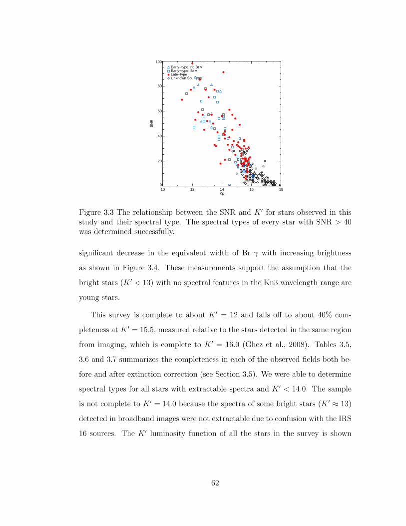
10 12 14 16 18Kp

0

20

40

60

80

100

SN

R

Early−type, no Br γEarly−type, Br γLate−typeUnknown Sp. Type

Figure 3.3 The relationship between the SNR and K ′ for stars observed in thisstudy and their spectral type. The spectral types of every star with SNR > 40was determined successfully.

significant decrease in the equivalent width of Br γ with increasing brightness

as shown in Figure 3.4. These measurements support the assumption that the

bright stars (K ′ < 13) with no spectral features in the Kn3 wavelength range are

young stars.

This survey is complete to about K ′ = 12 and falls off to about 40% com-

pleteness at K ′ = 15.5, measured relative to the stars detected in the same region

from imaging, which is complete to K ′ = 16.0 (Ghez et al., 2008). Tables 3.5,

3.6 and 3.7 summarizes the completeness in each of the observed fields both be-

fore and after extinction correction (see Section 3.5). We were able to determine

spectral types for all stars with extractable spectra and K ′ < 14.0. The sample

is not complete to K ′ = 14.0 because the spectra of some bright stars (K ′ ≈ 13)

detected in broadband images were not extractable due to confusion with the IRS

16 sources. The K ′ luminosity function of all the stars in the survey is shown

62

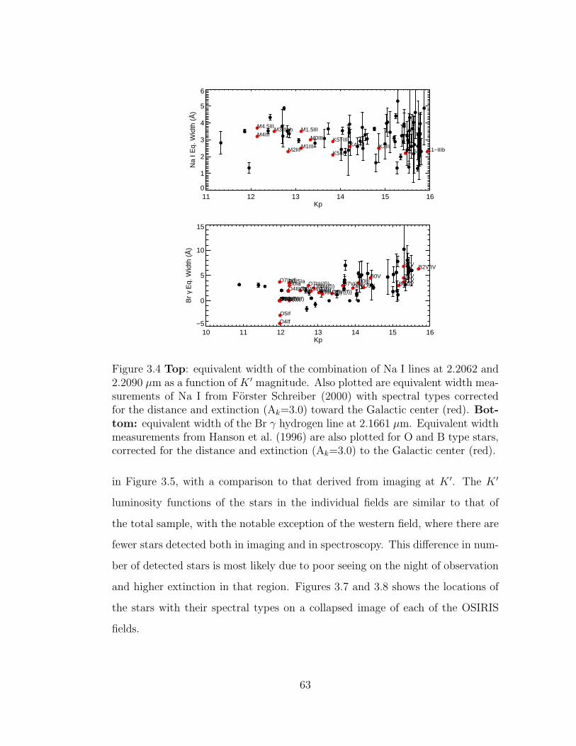
11 12 13 14 15 16Kp

0

1

2

3

4

5

6

Na

I Eq.

Wid

th (

Å)

K1−IIIbK2.5IIIK3IIIK4+III

K5−III

K5III

M0III

M1III

M1.5III

M2III

M3IIIabM4III

M4.5III

10 11 12 13 14 15 16Kp

−5

0

5

10

15

Br

γ E

q. W

idth

(Å

)

B0VB0III

B0Ib

B0Ia B0.5VB0.5IaB1V

B1V

B1V

B2V/IV

O3V

O3If

O4V((f))O4III(f)

O4If

O5V((f))

O5If

O6V{{f}}O6Ib(n)(f)

O7V((f))O7III((f))O7Ib(f)

O7Ib(f)

O8VO8III((f)) O9VO9III

O9Ia

Figure 3.4 Top: equivalent width of the combination of Na I lines at 2.2062 and2.2090 µm as a function of K ′ magnitude. Also plotted are equivalent width mea-surements of Na I from Forster Schreiber (2000) with spectral types correctedfor the distance and extinction (Ak=3.0) toward the Galactic center (red). Bot-

tom: equivalent width of the Br γ hydrogen line at 2.1661 µm. Equivalent widthmeasurements from Hanson et al. (1996) are also plotted for O and B type stars,corrected for the distance and extinction (Ak=3.0) to the Galactic center (red).

in Figure 3.5, with a comparison to that derived from imaging at K ′. The K ′

luminosity functions of the stars in the individual fields are similar to that of

the total sample, with the notable exception of the western field, where there are

fewer stars detected both in imaging and in spectroscopy. This difference in num-

ber of detected stars is most likely due to poor seeing on the night of observation

and higher extinction in that region. Figures 3.7 and 3.8 shows the locations of

the stars with their spectral types on a collapsed image of each of the OSIRIS

fields.

63

10 12 14 16Kp

0

20

40

60

80

100

120

140

Num

ber

of S

tars

WR stars

B0V

B2V

G5III

G8III

K0III

K2IIIK5III

M0III

M2III

M5III

O3I O3III O3V O5V O7V O9I O9V

−0.4

−0.2

0.0

0.2

0.4

H−

K

ImagingOld+YoungYoung StarsOld Stars

10 12 14 16Kp

0.0

0.2

0.4

0.6

0.8

1.0

Com

plet

enes

s

Figure 3.5 The K ′ luminosity function from the spectroscopic survey in compari-son to that found from imaging. In the top plot, we also include for reference, therough spectral types expected to be observable at each luminosity bin assumingAK = 3.0 and a distance of 8 kpc. The axis on the right shows the H-K colorassociated with each of the spectral types (Ducati et al., 2001; Martins & Plez,2006). The WR stars occupy a range in both K ′ and H-K colors.

64

central

10 12 14 16Kp

0

5

10

15

20

25

30

Num

ber

of S

tars

Old StarsYoung StarsOld+YoungImaging

east

10 12 14 16Kp

0

5

10

15

20

Num

ber

of S

tars

southeast

10 12 14 16Kp

0

5

10

15

20

Num

ber

of S

tars

south

10 12 14 16Kp

0

5

10

15

20

Num

ber

of S

tars

west

10 12 14 16Kp

0

2

4

6

8

10

12

Num

ber

of S

tars

north

10 12 14 16Kp

0

5

10

15

Num

ber

of S

tars

northeast

10 12 14 16Kp

0

2

4

6

8

10

12

Num

ber

of S

tars

southwest

10 12 14 16Kp

0

2

4

6

8

10

12

Num

ber

of S

tars

northwest

10 12 14 16Kp

0

2

4

6

8

Num

ber

of S

tars

Figure 3.6 The K ′ luminosity function from the spectroscopic survey in compar-ison to imaging in each individual pointing.

65

1 0 −1RA Offset (arcsec)

−1.5

−1.0

−0.5

0.0

0.5

1.0

1.5

Dec

Offs

et (

arcs

ec)

S0−1

S0−11

S0−14

S0−15S0−2S0−20S0−26S0−3

S0−30

S0−31

S0−38

S0−4S0−5

S0−7S0−8

S0−9

S1−1

S1−12

S1−14

S1−2

S1−22

S1−3

S1−33

S1−34

S1−4

S1−8

irs16C

irs16SW

S0−12

S0−13

S0−17

S0−18

S0−27

S0−28S0−29S0−6

S1−10

S1−13

S1−15S1−31

S1−5

S1−6

Central

1 0 −1RA Offset (arcsec)

−1.5

−1.0

−0.5

0.0

0.5

1.0

1.5

Dec

Offs

et (

arcs

ec)

S0−1

S0−11

S0−14

S0−15S0−2S0−20S0−26S0−3

S0−30

S0−31

S0−38

S0−4S0−5

S0−7S0−8

S0−9

S1−1

S1−12

S1−14

S1−2

S1−22

S1−3

S1−33

S1−34

S1−4

S1−8

irs16C

irs16SW

S0−12

S0−13

S0−17

S0−18

S0−27

S0−28S0−29S0−6

S1−10

S1−13

S1−15S1−31

S1−5

S1−6

Central, Br γ

4.0 3.5 3.0 2.5 2.0 1.5 1.0RA Offset (arcsec)

−1.5

−1.0

−0.5

0.0

0.5

Dec

Offs

et (

arcs

ec)

S2−22

S2−5

S2−58

S2−61

S2−64

S3−10

S3−3

S3−314

S3−34S3−5

irs16CC

irs16SW−E

S1−25S1−68S2−11

S2−31

S2−47

S2−65

S2−75

S2−83

S3−16

S3−36

S3−38

S3−383

S3−385

S3−6

S3−8

S4−1

East

4.0 3.5 3.0 2.5 2.0 1.5 1.0RA Offset (arcsec)

−1.5

−1.0

−0.5

0.0

0.5

Dec

Offs

et (

arcs

ec)

S2−22

S2−5

S2−58

S2−61

S2−64

S3−10

S3−3

S3−314

S3−34S3−5

irs16CC

irs16SW−E

S1−25S1−68S2−11

S2−31

S2−47

S2−65

S2−75

S2−83

S3−16

S3−36

S3−38

S3−383

S3−385

S3−6

S3−8

S4−1

East, Br γ

Figure 3.7 Images from collapsing the OSIRIS data cubes along the spectraldimension for each individual pointing of the survey. Right: median of all spec-tral channels. Left: spectral channels near the Br gamma line showing the gasemission. The images are oriented with north up and east to the left. Spec-troscopically identified early (blue triangles) and late-type (red circles) stars aremarked.

66

3.0 2.5 2.0 1.5 1.0 0.5RA Offset (arcsec)

−3.0

−2.5

−2.0

−1.5

−1.0

Dec

Offs

et (

arcs

ec)

S1−24

S1−34

S2−17

S2−29

S2−4S2−50

S2−55

S2−59

S2−6

S3−12

S3−30

S3−7

S2−25

S2−319

S2−73

S2−81

S3−11

S3−151 S3−20

S3−32

Southeast

3.0 2.5 2.0 1.5 1.0 0.5RA Offset (arcsec)

−3.0

−2.5

−2.0

−1.5

−1.0

Dec

Offs

et (

arcs

ec)

S1−24

S1−34

S2−17

S2−29

S2−4S2−50

S2−55

S2−59

S2−6

S3−12

S3−30

S3−7

S2−25

S2−319

S2−73

S2−81

S3−11

S3−151 S3−20

S3−32

Southeast, Br γ

0.5 0.0 −0.5 −1.0 −1.5 −2.0RA Offset (arcsec)

−3.0

−2.5

−2.0

−1.5

−1.0

Dec

Offs

et (

arcs

ec)

S1−12

S1−19 S2−21

S2−317

S2−77

S3−19

irs33N

S1−13

S1−17 S1−23

S1−36

S1−39

S1−48

S1−66

S1−67

S2−134

S2−18

S2−212

S2−3

S2−308

S2−41 S2−49 S2−57

S2−62

S2−71

S2−72

South

0.5 0.0 −0.5 −1.0 −1.5 −2.0RA Offset (arcsec)

−3.0

−2.5

−2.0

−1.5

−1.0

Dec

Offs

et (

arcs

ec)

S1−12

S1−19 S2−21

S2−317

S2−77

S3−19

irs33N

S1−13

S1−17 S1−23

S1−36

S1−39

S1−48

S1−66

S1−67

S2−134

S2−18

S2−212

S2−3

S2−308

S2−41 S2−49 S2−57

S2−62

S2−71

S2−72

South, Br γ

Figure 3.8 Similar to Figure 3.7, with additional OSIRIS fields.

67

−1.5 −2.0 −2.5 −3.0 −3.5 −4.0 −4.5RA Offset (arcsec)

−0.5

0.0

0.5

1.0

1.5

2.0

Dec

Offs

et (

arcs

ec)

S1−21

S3−190

irs34W

S2−70

S2−8

S3−109

S3−249

irs29S

West

−1.5 −2.0 −2.5 −3.0 −3.5 −4.0 −4.5RA Offset (arcsec)

−0.5

0.0

0.5

1.0

1.5

2.0

Dec

Offs

et (

arcs

ec)

S1−21

S3−190

irs34W

S2−70

S2−8

S3−109

S3−249

irs29S

West, Br γ

1.5 1.0 0.5 0.0 −0.5 −1.0RA Offset (arcsec)

1.0

1.5

2.0

2.5

3.0

Dec

Offs

et (

arcs

ec)

S1−18

S2−19

S2−7

S2−74 S2−76

irs16NW

S1−20S1−44

S2−2

S2−205

S2−26

S2−32

S2−37S2−51

S3−14 S3−68North

1.5 1.0 0.5 0.0 −0.5 −1.0RA Offset (arcsec)

1.0

1.5

2.0

2.5

3.0

Dec

Offs

et (

arcs

ec)

S1−18

S2−19

S2−7

S2−74 S2−76

irs16NW

S1−20S1−44

S2−2

S2−205

S2−26

S2−32

S2−37S2−51

S3−14 S3−68North, Br γ


68

4.0 3.5 3.0 2.5 2.0 1.5RA Offset (arcsec)

0.5

1.0

1.5

2.0

2.5

Dec

Offs

et (

arcs

ec)

S2−40

S3−2irs16CC

irs16NE

S2−12

S2−23

S2−34

S2−80

S3−37

S3−39

S4−2

Northeast

4.0 3.5 3.0 2.5 2.0 1.5RA Offset (arcsec)

0.5

1.0

1.5

2.0

2.5

Dec

Offs

et (

arcs

ec)

S2−40

S3−2irs16CC

irs16NE

S2−12

S2−23

S2−34

S2−80

S3−37

S3−39

S4−2

Northeast, Br γ

−1.0 −1.5 −2.0 −2.5 −3.0 −3.5RA Offset (arcsec)

1.5

2.0

2.5

3.0

3.5

Dec

Offs

et (

arcs

ec)

S2−16S2−66

S3−17 S4−12

irs29N

S2−85

S3−149

S3−262S3−284

S3−288S4−59

S4−84

Northwest

−1.0 −1.5 −2.0 −2.5 −3.0 −3.5RA Offset (arcsec)

1.5

2.0

2.5

3.0

3.5

Dec

Offs

et (

arcs

ec)

S2−16S2−66

S3−17 S4−12

irs29N

S2−85

S3−149

S3−262S3−284

S3−288S4−59

S4−84

Northwest, Br γ


69

−1.5 −2.0 −2.5 −3.0 −3.5 −4.0 −4.5RA Offset (arcsec)

−2.0

−1.5

−1.0

−0.5

0.0

Dec

Offs

et (

arcs

ec)

S1−22S3−96

irs13E1irs13E2

irs13E4

S2−24S2−67

S2−78

S3−187

S3−291

Southwest

−1.5 −2.0 −2.5 −3.0 −3.5 −4.0 −4.5RA Offset (arcsec)

−2.0

−1.5

−1.0

−0.5

0.0

Dec

Offs

et (

arcs

ec)

S1−22S3−96

irs13E1irs13E2

irs13E4

S2−24S2−67

S2−78

S3−187

S3−291

Southwest, Br γ


70

Table 3.2. OSIRIS observations of late-type stars

Name K′ RA offset DEC offset R Epoch Notea Na σNa Nobsb SNRc Field

(′′) (′′) (′′) (A) (A)

S0-17 15.70 0.02 -0.09 0.10 2004.47 4 1.30 0.17 11 20 CS0-6 14.20 0.05 -0.38 0.39 2002.69 4 2.92 0.83 9 44 CS0-27 15.70 0.14 0.53 0.54 2003.34 1 3.80 0.41 6 12 CS0-29 15.60 0.32 -0.46 0.56 2004.84 4 4.63 1.40 9 6 CS0-28 15.80 -0.17 -0.55 0.57 2003.53 4 2.13 1.50 8 31 CS0-12 14.40 -0.56 0.39 0.68 2002.69 4 2.60 0.51 4 33 CS0-13 13.50 0.54 -0.44 0.69 2002.69 4 2.80 0.24 6 77 CS1-5 12.80 0.34 -0.92 0.98 2002.69 4 3.22 0.64 4 45 CS1-10 14.90 -1.13 -0.03 1.13 2002.99 4 2.50 0.86 5 25 CS1-31 15.70 -0.98 0.56 1.13 2003.60 1 4.62 1.53 4 11 CS1-6 15.50 -0.93 0.73 1.18 2003.34 1 3.54 1.01 2 18 CS1-36 15.80 -0.63 -1.20 1.35 2003.58 1 2.31 0.77 4 18 SS1-13 14.20 -1.12 -0.92 1.45 2002.91 4 2.38 1.50 3 21 CS1-15 14.20 -1.36 0.52 1.45 2002.69 1 3.42 0.27 4 38 CS1-39 15.40 -0.55 -1.37 1.48 2003.22 1 3.94 0.66 7 16 SS1-17 12.50 0.47 -1.49 1.56 2002.69 1 4.33 0.17 4 85 SS1-44 15.60 0.30 1.61 1.63 2003.48 1 4.03 0.40 5 22 NS1-48 15.50 -0.62 -1.53 1.66 2004.20 1 3.23 0.87 10 32 SS1-20 12.70 0.41 1.61 1.66 2002.69 1 4.87 0.12 12 57 NS1-23 11.90 -0.93 -1.48 1.74 2002.69 1 3.51 0.10 10 77 SS1-25 13.50 1.65 -0.63 1.76 2002.69 3 3.51 · · · 1 33 ES1-66 15.60 -0.81 -1.76 1.94 2004.87 1 1.38 0.37 10 8 SS1-67 15.60 -1.44 -1.32 1.95 2003.56 1 2.61 0.72 9 30 SS1-68 13.40 1.86 -0.61 1.96 2002.69 1 2.47 0.52 4 50 ES2-12 15.30 1.67 1.17 2.04 2003.08 1 4.41 0.16 5 18 NES2-34 15.40 1.81 0.97 2.05 2003.43 1 3.80 1.00 5 18 NES2-11 12.00 1.97 -0.62 2.07 2002.69 1 1.33 0.33 8 98 ES2-3 14.50 -1.54 -1.41 2.09 2002.84 1 2.92 0.23 9 61 SS2-37 15.80 0.08 2.10 2.11 2003.91 1 3.14 0.55 12 17 NS2-2 14.10 -0.55 2.06 2.13 2002.88 1 2.26 0.21 11 42 NS2-41 15.50 -0.47 -2.10 2.16 2004.41 1 2.86 1.30 10 36 SS2-8 12.20 -1.84 0.96 2.08 2002.69 1 2.82 0.66 9 53 W

71

Table 3.2—Continued


(′′) (′′) (′′) (A) (A)

S2-134 15.60 -0.99 -1.99 2.23 2005.79 1 3.66 0.84 10 8 SS2-49 15.50 -0.83 -2.10 2.26 2004.14 1 2.88 0.46 10 19 SS2-47 14.20 2.19 -0.53 2.25 2002.75 1 2.84 0.79 10 41 ES2-51 15.90 0.76 2.18 2.31 2004.88 1 4.88 2.19 12 23 NS2-18 13.30 -0.98 -2.14 2.35 2002.83 3 3.18 0.17 10 57 SS2-23 14.80 1.66 1.77 2.42 2002.93 1 3.64 0.38 4 36 NES2-57 14.70 -1.21 -2.12 2.44 2003.76 1 3.06 0.30 10 45 SS2-24 13.80 -2.33 -0.90 2.50 2003.30 7 6.05 1.72 4 18 SWS2-26 13.70 0.74 2.42 2.53 2002.65 3 3.65 0.34 12 43 NS2-62 15.20 -1.07 -2.32 2.56 2004.67 1 2.89 0.37 10 31 SS2-25 14.10 0.74 -2.45 2.56 2003.50 1 3.54 0.21 8 91 SES2-205 15.80 0.48 2.51 2.56 2005.54 1 3.34 1.31 12 22 NS2-65 15.80 2.35 -1.06 2.58 2004.13 1 1.96 0.22 10 18 ES2-212 15.70 0.18 -2.59 2.59 2006.75 1 3.31 2.01 7 12 SS2-67 13.80 -2.50 -0.85 2.63 2003.29 7 6.59 0.75 4 28 SWS2-70 14.50 -2.64 0.41 2.67 2003.98 1 3.74 0.90 11 29 WS2-71 15.30 -0.90 -2.53 2.68 2004.72 1 1.99 0.16 10 30 SS2-72 15.10 -1.46 -2.28 2.71 2004.32 1 3.98 0.51 10 32 SS2-73 15.20 2.16 -1.64 2.72 2003.15 1 3.09 0.12 11 49 SES2-75 14.50 2.63 -0.89 2.78 2002.69 1 2.49 0.70 10 39 ES2-31 13.10 2.81 -0.20 2.81 2002.69 1 2.96 0.12 10 71 ES2-78 13.80 -2.81 -0.29 2.82 2003.53 7 4.49 0.73 3 34 SWS2-80 15.60 2.23 1.78 2.85 2003.58 1 2.40 0.91 5 20 NES2-81 15.60 1.97 -2.07 2.86 2004.75 1 2.98 0.53 11 22 SES2-83 15.60 2.86 -0.69 2.94 2003.62 1 2.17 1.70 10 21 ES2-319 15.70 0.99 -2.79 2.96 2005.71 1 2.62 0.81 8 14 SES2-85 12.20 -1.26 2.70 2.98 2003.64 7 4.98 0.16 5 55 NWS2-32 12.40 1.12 2.78 2.99 2003.05 1 3.53 0.15 6 59 NS3-68 15.80 -0.35 3.06 3.08 2005.93 1 3.96 0.53 5 21 NS3-14 13.90 0.10 3.09 3.09 2004.54 1 1.98 · · · 1 18 NS3-16 15.30 2.99 -0.95 3.13 2003.76 1 5.30 1.30 10 24 ES3-20 14.90 1.58 -2.80 3.21 2003.83 1 1.64 0.53 11 54 SE

72



(′′) (′′) (′′) (A) (A)

S3-6 12.90 3.22 0.01 3.22 2002.80 1 3.36 0.26 10 77 ES3-109 15.60 -3.20 0.43 3.23 2006.75 1 4.32 1.96 11 20 WS3-149 13.30 -2.92 1.68 3.37 2005.93 7 4.52 0.08 3 23 NWS3-151 15.70 1.90 -2.78 3.37 2006.22 1 2.99 1.56 11 16 SES3-32 15.50 2.91 -1.77 3.41 2004.51 1 3.24 0.62 9 37 SES3-8 14.00 3.41 -0.49 3.44 2002.81 1 2.43 0.67 10 56 ES3-187 14.40 -3.40 -0.74 3.48 2006.75 7 -4.66 1.12 4 13 SWS3-11 15.10 2.96 -1.93 3.53 2004.12 3 4.05 0.84 4 35 SES3-36 14.70 3.46 -0.83 3.55 2003.76 1 3.65 0.11 9 57 ES3-249 14.70 -3.38 1.32 3.63 2006.75 1 3.30 0.34 11 33 WS3-37 15.10 3.39 1.35 3.65 2004.66 1 3.45 1.23 5 17 NES3-262 15.10 -2.34 2.83 3.67 2006.75 7 3.77 0.25 6 26 NWS3-38 15.00 3.69 -0.11 3.69 2005.34 1 2.76 0.92 9 33 ES3-39 13.60 3.57 1.10 3.73 2002.97 1 3.08 0.53 3 32 NES3-284 13.70 -2.58 2.72 3.74 2006.75 7 5.43 0.33 6 53 NWS3-288 14.30 -2.77 2.54 3.76 2006.75 7 5.49 0.19 6 44 NWS3-291 12.20 -3.55 -1.26 3.76 2006.58 7 5.59 0.38 4 46 SWS3-385 15.30 3.67 -1.50 3.96 2005.81 1 1.32 0.36 6 26 ES4-1 13.50 4.02 -0.37 4.04 2003.92 1 3.09 0.25 9 102 ES4-2 13.00 3.75 1.67 4.10 2004.01 1 3.51 0.33 3 52 NES4-59 13.70 -3.16 2.65 4.13 2006.75 7 3.50 0.09 6 38 NWS4-84 14.00 -3.35 2.49 4.18 2006.75 7 5.53 0.24 2 31 NW

a1. Spectral type first reported in this work. Recent spectral identification: 2. Paumard et al. (2006) 3.Genzel et al. (2000) 4. Gillessen et al. (2009)

bEach observation has an integration time of 900 s.

cSignal to noise per pixel calculated between 2.212 to 2.218 µm.

73

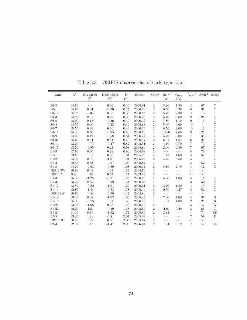
Table 3.3. OSIRIS observations of early-type stars

Name K′ RA offset DEC offset R Epoch Notea Br γb σBrγ Nobsc SNRd Field

(′′) (′′) (′′) (A) (A)

S0-2 14.10 · · · 0.16 0.16 2005.61 2 3.90 1.50 11 67 CS0-1 14.70 0.04 -0.26 0.27 2006.30 2 0.50 0.30 9 31 CS0-19 15.50 -0.04 0.35 0.35 2006.25 2 5.70 2.30 11 16 CS0-3 14.50 0.31 0.12 0.33 2006.38 2 5.40 3.60 9 21 CS0-5 15.10 0.18 -0.36 0.40 2006.32 2 7.80 1.10 9 15 CS0-4 14.50 0.40 -0.28 0.49 2005.83 2 5.40 6.00 10 1 CS0-7 15.50 0.49 0.10 0.49 2006.36 2 6.50 2.00 10 12 CS0-11 15.30 0.50 -0.05 0.50 2006.73 2 10.20 7.60 9 21 CS0-9 14.40 0.19 -0.58 0.61 2006.74 4 5.40 2.00 7 38 CS0-31 15.10 0.54 0.44 0.70 2006.47 2 6.01 1.54 6 21 CS0-14 13.70 -0.77 -0.27 0.82 2005.51 2 4.10 0.70 7 76 CS0-15 13.70 -0.95 0.24 0.98 2005.80 2 2.40 0.50 7 67 CS1-3 12.10 0.40 0.88 0.96 2004.98 2 · · · · · · 5 79 CS1-1 13.10 1.01 0.03 1.01 2005.20 4 1.72 1.00 5 57 CS1-2 14.90 0.01 -1.01 1.01 2005.93 2 4.70 3.50 5 19 CS1-4 12.60 0.83 -0.67 1.06 2005.84 1 · · · · · · 5 52 CS1-8 14.20 -0.63 -0.89 1.08 2006.17 2 5.10 2.70 4 42 CIRS16NW 10.10 0.05 1.22 1.22 2004.74 2 · · · · · · · · · · · ·IRS16C 9.90 1.10 0.51 1.21 2003.89 2 · · · · · · · · · · · ·S1-33 15.00 -1.25 -0.01 1.25 2006.26 1 5.20 1.60 5 17 CS1-34 13.20 0.85 -0.99 1.31 2006.38 1 · · · · · · 3 52 CS1-12 13.80 -0.80 -1.01 1.29 2006.21 2 3.70 1.50 4 40 CS1-14 12.80 -1.34 -0.33 1.38 2005.49 6 0.50 0.27 3 52 CIRS16SW 10.10 1.06 -0.96 1.44 2004.89 2 · · · · · · · · · · · ·S1-19 13.80 0.38 -1.62 1.66 2005.45 1 7.00 1.00 4 37 SS1-18 15.00 -0.76 1.51 1.69 2006.56 1 1.81 1.00 2 24 NS1-21 13.30 -1.66 0.13 1.66 2006.16 2 · · · · · · 5 47 WS1-22 12.70 -1.61 -0.49 1.68 2005.65 2 -1.61 0.49 3 61 CS1-24 11.60 0.71 -1.62 1.77 2005.64 2 2.84 · · · 1 74 SES2-5 13.30 1.91 -0.81 2.07 2005.68 1 · · · · · · 7 58 EIRS16CC 10.60 1.99 0.56 2.06 2004.57 2 · · · · · · · · · · · ·S2-4 12.30 1.47 -1.47 2.08 2006.04 2 1.94 0.19 11 149 SE

74



(′′) (′′) (′′) (A) (A)

S2-6 12.00 1.61 -1.35 2.10 2004.69 2 2.04 0.16 7 103 SES2-7 14.10 0.95 1.84 2.08 2006.15 2 · · · · · · 12 54 NIRS29N 10.30 -1.58 1.41 2.12 2005.07 2 · · · · · · · · · · · · NWIRS16SW-E 11.00 1.86 -1.14 2.18 2005.52 2 · · · · · · · · · · · ·IRS33N 11.40 -0.05 -2.21 2.21 2006.19 2 3.10 0.40 10 104 SS2-17 10.90 1.29 -1.88 2.28 2005.14 2 3.19 0.07 11 125 SES2-50 15.50 1.68 -1.52 2.26 2005.38 1 8.00 3.00 11 16 SES2-16 11.90 -1.02 2.07 2.31 2005.40 2 · · · · · · 1 41 NWS2-22 12.90 2.30 -0.24 2.31 2005.33 6 -0.73 0.50 10 78 ES2-19 12.60 0.42 2.31 2.34 2005.53 2 2.04 0.50 12 68 NS2-21 13.50 -1.66 -1.64 2.34 2006.34 1 1.20 0.70 8 71 SS2-55 15.40 0.88 -2.19 2.36 2006.53 1 3.20 1.20 11 29 SES2-58 14.10 2.14 -1.16 2.43 2005.74 1 4.70 3.00 7 41 ES2-59 15.40 0.79 -2.33 2.46 2006.48 1 5.60 2.00 10 25 SES2-61 15.50 2.37 -0.67 2.47 2006.56 1 6.00 3.00 10 16 ES2-74 13.30 0.15 2.78 2.78 2006.16 2 · · · · · · 12 81 NS2-77 13.80 -1.78 -2.19 2.82 2006.16 1 1.40 0.50 9 54 SS2-76 15.20 -0.23 2.81 2.82 2006.76 1 1.18 1.00 12 38 NS2-317 15.60 -0.74 -2.86 2.95 2006.40 1 5.10 1.00 3 21 SIRS16NE 9.10 2.87 1.01 3.04 2003.62 2 · · · · · · · · · · · ·S3-2 12.10 3.06 0.53 3.11 2005.43 1 0.49 0.04 3 47 NES3-3 15.10 3.06 -0.67 3.14 2006.47 1 1.90 2.00 10 21 ES3-5 12.20 2.94 -1.18 3.16 2005.66 2 · · · · · · 10 87 ES3-17 14.10 -1.42 2.86 3.19 2006.60 7 · · · · · · · · · · · · NWS3-96 14.50 -3.13 -0.62 3.19 2006.82 2 · · · · · · 4 28 SWS3-7 13.90 1.91 -2.61 3.23 2006.34 1 · · · · · · 11 76 SEIRS13E1 10.90 -2.97 -1.63 3.39 2006.50 2 5.17 1.04 4 108 SWS3-30 12.80 1.64 -2.96 3.38 2006.39 2 1.63 0.44 8 56 SES3-34 13.50 3.22 -1.26 3.46 2006.29 1 2.12 1.28 9 46 ES3-190 14.10 -3.17 1.45 3.49 2006.47 1 1.20 1.10 11 55 WIRS13E4 12.00 -3.22 -1.39 3.51 2006.23 2 · · · · · · 4 66 SWS3-10 12.40 3.33 -1.14 3.52 2005.99 2 · · · · · · 10 81 E

75



(′′) (′′) (′′) (A) (A)

S3-12 12.00 2.37 -2.73 3.61 2001.39 1 · · · · · · 11 114 SEIRS13E2 10.80 -3.19 -1.71 3.62 2006.35 2 · · · · · · 3 36 SWS3-314 15.40 3.81 -0.12 3.82 2006.43 1 6.80 2.60 9 26 ES4-12 14.90 -2.82 2.86 4.02 2006.40 7 · · · · · · · · · · · · NW

a1. Spectral type first reported in this work. Recent spectral identification: 2. Paumard et al. (2006) 3. Genzelet al. (2000) 4. Gillessen et al. (2009) 5. Bartko et al. (2009).

bEach observation has an integration time of 900 s.

cStars with no reported equivalent widths have no detectable Br γ lines (see Section 3.4), with the exception ofthe IRS 16 sources, which all have strong Br γ emission lines from strong winds.

dSignal to noise per pixel calculated between 2.212 to 2.218 µm.

Table 3.4. OSIRIS spectra with unknown spectral type

Name K′ RA offset DEC offset R Epoch SNRa

(′′) (′′) (′′)

S0-35 15.3 0.06 0.97 0.97 2003.77 16S1-26 15.6 -0.92 0.39 1 2003.07 12S1-29 15.4 1.08 0.17 1.09 2005.09 11S1-32 15.3 -0.96 -0.64 1.15 2003.21 20S1-7 15.9 -1.03 -0.53 1.16 2003.86 13S1-85 15.5 0.92 -0.82 1.23 2006.75 4S1-40 15.9 -1.39 -0.62 1.52 2004.23 7S1-41 15.8 0.99 1.15 1.52 2003.69 4S1-42 15.9 0.94 1.26 1.57 2004.04 9S1-45 15.3 -1.27 1.04 1.65 2003.04 13S1-47 15.6 -1.58 0.46 1.65 2003.14 1S1-50 15.4 1.5 0.68 1.65 2003.7 9S1-128 15.8 1.33 -0.99 1.66 2006.55 0S1-51 15 -1.65 -0.18 1.66 2002.99 10S1-52 15.2 0 1.67 1.67 2003.15 28S1-53 15.3 1.67 -0.12 1.67 2003.12 11S1-54 15.5 -1.52 0.74 1.69 2004.25 3S1-55 15.5 1.59 0.6 1.69 2004.17 7S1-56 15.8 -1.11 1.35 1.75 2003.85 11S1-61 15.9 -1.49 -1 1.79 2003.96 6S1-62 15.3 0.5 1.75 1.82 2003.21 19S1-59 15.5 0.02 1.82 1.82 2003.33 27S1-147 15.9 1.18 -1.47 1.89 2006.75 7S1-64 15.5 0.64 1.81 1.92 2003.08 13S1-159 15.9 1.3 -1.43 1.93 2005.94 9S1-65 15.7 1.46 1.27 1.93 2003.85 5S2-89 15.9 1.07 -1.7 2.01 2006.75 5S2-42 15.6 0.46 2.1 2.15 2004.02 23S2-200 15.7 -2.53 0 2.53 2005.25 12S2-63 15.4 -0.65 2.48 2.56 2003.98 12S2-219 15.8 -1.6 -2.07 2.62 2005.34 8S2-261 15.6 -2.61 1 2.8 2006.04 11

76


Name K′ RA offset DEC offset R Epoch SNRa

(′′) (′′) (′′)

S2-268 15.5 -2.78 0.49 2.82 2006.32 13S2-304 15.9 2.52 1.47 2.91 2006.39 12S2-306 15.6 -0.48 -2.89 2.93 2006.75 17S2-84 15.6 1.65 -2.47 2.97 2004.29 26S3-48 15.9 -3 0.37 3.02 2006.32 15S3-50 15.7 -1.87 -2.38 3.03 2006.75 13S3-51 15.1 -0.15 3.02 3.03 2005.88 15S3-62 15.7 2.68 -1.48 3.06 2006.4 28S3-65 15.7 -1.27 -2.8 3.07 2005.72 11S3-4 14.7 3.08 -0.52 3.13 2002.91 28S3-90 15.8 2.74 -1.56 3.15 2005.21 30S3-91 15.7 -1.73 -2.67 3.18 2006.75 8S3-116 15.9 2.25 2.37 3.27 2006.11 9S3-24 15.6 3.26 0.41 3.29 2004.87 4S3-167 15.5 -3.08 1.42 3.4 2006.75 16S3-169 15.5 -3.39 0.38 3.41 2006.75 27S3-31 15.5 3.4 0.38 3.42 2004.42 7S3-33 15.4 3.32 -0.85 3.43 2004.25 16S3-286 15.3 3.42 -1.54 3.75 2004.66 13S3-319 15.4 3.55 -1.42 3.83 2006.39 17S4-47 15.9 2.56 -3.23 4.12 2006.75 11S4-67 15.7 2.8 -3.05 4.14 2006.75 7

aSignal to noise per pixel calculated between 2.212 to 2.218 µm.

3.5 Results

With spectroscopic identification of the stars brighter than K ′ ∼ 15.5, we are

able to separate the presumably dynamically relaxed old stars from the unrelaxed

young population. The stellar number density profile is constructed in radial bins

of 0.′′5 over the area that was sampled in this survey out to a radius of ∼ 3′′, with

error bars scaling as√

N , where N is the number of stars in each bin. It is clear

that, while the number density of early-type stars increases quite rapidly toward

the central arcsecond, the late-type stars have a very flat distribution (Figure

3.12). Outside the central arcsecond, the projected number density of early-type

stars drops to about half that of the late-type stars. For a quantitative comparison

to stellar cusp models, we fit a power law to the surface number density of both

populations. The late-type population is best fit with a power law slope Γold =

77

1Radius (arcsec)

0.1

1.0

10.0

100.0

N s

tars

/ ar

csec

2

Young Stars Γ =1.47±0.22Old Stars Γ =0.06±0.18All Stars Γ =0.15±0.07

Figure 3.12 Plot of the surface number density as a function of projected distancefrom Sgr A* in the plane of the sky for different populations: old (late-type, red),young (early-type, blue), and total number counts from K ′ imaging.

0.06±0.18, while for the early-type stars, Γyoung = 0.97±0.28. For comparison, we

also measured the projected stellar number density over the same survey region

using LGS AO K ′ imaging from July 2008, which is much deeper (K ′ < 20),

but with no spectroscopic discrimination. We find that Γimaging = 0.15 ± 0.07,

comparable to that found by Schodel et al. (2007) using only number counts. The

spectroscopically determined late-type slope is flatter than that determined from

number counts alone, but is consistent within the ∼ 2σ formal fitting errors.

The survey has complete azimuthal coverage out to a radial distance of ∼ 1.′′5

from Sgr A*. Beyond this radius, the radial coverage extends out to ∼ 4′′, but

the azimuthal coverage is complete due to two fields missing in the northwest

and southwest. We find that these missing two fields do not significantly impact

78

Table 3.5. Results and survey completeness

Observed AK Correctedd

Field NSFa NID

b Akc RMSAk

K′e Completeness K′ Completeness

C 100 28 3.24 0.04 15.5 - 16.0 0.4 15.5 - 16.0 0.4E 37 25 3.05 0.06 15.5 - 16.0 0.3 15.0 - 15.5 0.3SE 60 25 3.29 0.10 15.5 - 16.0 0.4 15.0 - 15.5 0.5S 35 6 3.28 0.05 15.5 - 16.0 0.6 15.0 - 15.5 0.6W 35 19 3.44 0.12 14.5 - 15.0 0.7 14.0 - 14.5 0.4N 40 14 3.39 0.12 15.5 - 16.0 0.4 15.0 - 15.5 0.4

NE 32 7 3.13 0.07 15.0 - 15.5 0.5 15.0 - 15.5 0.5SW 32 10 3.43 0.20 14.5 - 15.0 0.3 14.0 - 14.5 0.4NW 65 11 3.68 0.10 15.0 - 15.5 0.4 14.0 - 14.5 0.8

aNumber of stars detected by StarFinder.

bNumber of stars with determined spectral types.

cExtinction values from Buchholz et al. (2009).

dExtinction correction using (Ak - 3.0), with Ak from the extinction map in Buchholz et al. (2009).

eFaintest magnitude bin where the completeness is at least 30%.

the radial profile of the late-type stars, as removing one or two of the outer

observed fields from the analysis leads to the same power law slope, within the

measurement uncertainties. In addition, previous observations of the late-type

stars in this region have found the distribution to be isotropic (e.g. Genzel et al.,

2003b; Trippe et al., 2008).

Potential systematic errors to the radial profile measurement may arise from

variable extinction and incompleteness between each field. In order to study

how these two factors impact our result, the radial profile was computed using

stars with extinction corrected magnitudes only over regions that are at least

30% complete. To do so, the extinction map reported by Buchholz et al. (2009)

was used to correct for the variations in extinction between each star by adding

AK − 3.0 to each star to bring them to the same canonical AK = 3.0 extinction

to the Galactic center (see Table 3.5 for the average and RMS value of AK in

each field). Then, the K ′ luminosity function was recomputed for each field to

79

Table 3.6. Field Completeness

Magnitude Bina Central E SE S W N NE SW NW

9.00 0.00 0.00 0.00 0.00 0.00 0.00 1.00 0.00 0.009.50 1.00 0.00 0.00 0.00 0.00 0.00 0.00 0.00 0.0010.00 1.00 0.00 0.00 0.00 0.00 1.00 0.00 0.00 1.0010.50 0.00 0.00 1.00 0.00 0.00 0.00 1.00 1.00 0.0011.00 0.00 1.00 0.00 1.00 1.00 0.00 0.00 0.00 0.0011.50 0.00 0.00 1.00 1.00 0.00 0.00 0.00 0.00 1.0012.00 1.00 1.00 1.00 0.00 1.00 0.00 1.00 1.00 1.0012.50 1.00 1.00 1.00 1.00 0.00 1.00 0.00 1.00 0.0013.00 1.00 0.75 0.00 1.00 0.00 1.00 0.50 0.00 0.0013.50 0.75 1.00 1.00 1.00 0.00 1.00 0.50 1.00 0.5014.00 0.67 0.75 0.50 0.00 0.50 1.00 0.00 1.00 1.0014.50 0.83 0.50 0.33 0.67 0.67 0.00 1.00 0.33 0.5015.00 0.36 0.38 0.43 0.67 0.00 0.33 0.50 0.00 0.4015.50 0.41 0.29 0.38 0.59 0.08 0.38 0.17 0.00 0.0016.00 0.20 0.00 0.00 0.00 0.00 0.00 0.00 0.00 0.00

aLeft side of the magnitude bin.

Table 3.7. Extinction Corrected Field Completeness

Magnitude Bina Central E SE S W N NE SW NW

9.00 0.00 0.00 0.00 0.00 0.00 0.00 0.00 0.00 0.009.50 1.00 0.00 0.00 0.00 0.00 1.00 0.00 0.00 1.0010.00 0.00 0.00 0.00 0.00 0.00 0.00 1.00 1.00 0.0010.50 0.00 1.00 1.00 0.00 1.00 0.00 0.00 1.00 0.0011.00 0.00 0.00 1.00 1.00 0.00 0.00 0.00 1.00 1.0011.50 1.00 1.00 1.00 1.00 1.00 0.00 0.00 1.00 1.0012.00 1.00 1.00 1.00 1.00 0.00 1.00 1.00 1.00 0.0012.50 1.00 1.00 0.00 1.00 0.00 1.00 0.33 0.00 0.0013.00 1.00 0.80 0.00 1.00 0.00 1.00 0.00 0.00 0.6713.50 0.67 1.00 0.67 1.00 1.00 1.00 1.00 1.00 1.0014.00 0.71 0.75 0.00 0.50 0.40 0.00 0.00 0.40 0.7514.50 0.83 0.50 0.33 0.75 0.00 0.33 0.50 0.00 0.0015.00 0.36 0.33 0.47 0.62 0.09 0.40 0.45 0.00 0.0015.50 0.31 0.25 0.00 0.14 0.00 0.10 0.00 0.00 0.0016.00 0.00 0.00 0.00 0.00 0.00 0.00 0.00 0.00 0.0016.50 0.07 0.00 0.00 0.00 0.00 0.00 0.00 0.00 0.00

aLeft side of the magnitude bin.

80

1Radius (arcsec)

0.1

1.0

10.0

100.0

N s

tars

/ ar

csec

2

Young Stars Γ =0.90±0.29Old Stars Γ =−0.26±0.24All Stars Γ =0.15±0.07

Figure 3.13 Plot of the surface number density as a function of projected distancefrom Sgr A* in the plane of the sky for different populations: old (late-type, red),young (early-type, blue), and total number counts from K ′ imaging. These radialprofiles have been corrected for completeness and extinction using the methoddetailed in Section 3.5.

determine the K ′ magnitude bin beyond which the completeness falls to less

than 30%. Table 3.5 shows this magnitude bin for each field before and after

extinction correction. This separates the fields into three groups in terms of their

30% completeness : all fields are at least 30% complete down to K ′ = 14.5; all

fields except W, SW, and NW are complete to K ′ = 15.5; the central field is

complete to K ′ = 16.0. We calculate the radial profiles in each magnitude bin

using only fields that are at least 30% complete at that magnitude. For all stars

with K ′ < 14.5, we use all the fields, while for stars with 14.5 ≤ K ′ < 15.5,

the western field was dropped from the measurement; the 15.5 ≤ K ′ < 16.0

magnitude bin was not included because only the central field is complete to at

81

least 30% at that magnitude. The radial profiles from the K ′ < 14.5 and 14.5 ≤K ′ < 15.5 magnitude bins were then summed to produce the final measurement

of the surface density, with errors added in quadrature (see Figure 3.13). A total

of 60 early-type and 69 late-type stars are included in the final radial profile

measurement. The early-type stars have Γyoung = 0.90± 0.29, while for the late-

type stars, Γold = −0.26 ± 0.24. Neither of these values differ significantly from

the case without extinction and completeness correction. The rest of the analysis

will use these values for the measured surface number density profile.

Beyond a radius of 1′′, there are more young stars detected in the eastern and

southeastern fields compared to the other observed regions. This excess is in the

direction of the major axis of the projected coherent disk of young stars orbiting

in the clockwise direction in the plane of the sky (Lu et al., 2009). however, after

accounting for the completeness and differences in AK , neither the number of

young, nor old stars shows a statistically significant excess.

3.6 Discussion

The effects of projection of a three-dimensional cluster onto the plane of the sky

must be taken into account for quantitative interpretations of the measured sur-

face density profile. The projection onto the sky plane of a spherically symmetric

cluster can be done using the integral:

Σ(R) = 2

∫ ∞

R

rn(r)dr√r2 − R2

(3.1)

where R is the distance from the center of the cluster in the plane of the sky, r is

the physical radius of the star cluster, Σ(R) is the projected surface density, and

n(r) is the volume number density. Because this integral diverges for all γ < 1.0,

82

0.01 0.10 1.00 10.00r (arcsec)

0.01

0.10

1.00

10.00

100.00

n(r)

γ1 = −0.5γ1 = 0.0γ1 = 0.5γ1 = 1.0

0.01 0.10 1.00 10.00Projected Radius (arcsec)

0.1

1.0

10.0

100.0

Σ(R

)

Γ = 0.18Γ = 0.04Γ = 0.01Γ = −0.01

Figure 3.14 Left: broken power law density profiles with break radius, rbreak =8.0′′ and outer power law γ2 = 2.0, and varying inner power laws γ1. Right: theprojected surface number density profile of each of the broken power laws. Thefitted inner surface density power law Γ is flat for γ1 ∼< 0.5.

where n(r) ∝ r−γ, the density in the outer region of the cluster must fall off

steeply to accommodate a shallow power law at the center of the cluster. While

we do not observe a break in the cluster density profile within our 4′′ survey, one

was observed by Schodel et al. (2007) and others at scales larger than our survey.

In order to account for the outer region of the star cluster, we therefore model

the number density profile as a broken power law:

n(r) ∝

r−γ1 r < rbreak,

r−γ2 r ≥ rbreak.(3.2)

Using the measurements from Schodel et al. (2007), we set rbreak = 8′′ and γ2 = 1.8

(the deprojected values of Rbreak = 6′′ and Γ = 0.8, from the surface density

measurements using this broken power law model) to constrain the parameters

of the outer cluster density profile. We assumed that contamination from young

stars is less severe in the region outside of our survey, so using an outer cluster

density profile measured from total number counts should introduce only a small

bias. For example, the density of bright young stars falls off relatively steeply as

83

R−2 (Paumard et al., 2006; Lu et al., 2009, but see also Buchholz et al. (2009)).

To determine the constraints on the physical density profile in the inner region,

we performed Monte Carlo simulations of clusters with γ1 between -2.0 and 2.0.

For each value of γ1, 104 realizations were performed. In each realization, 69 stars

(the number of late-type stars used to measure the radial profile) were drawn from

the broken power law distribution after correcting for the limited area observed

in this survey. The locations of these stars were then binned and fitted the same

way as the data. We find that for −2.0 < γ1 < 0.5, the projected inner radial

profiles are flat with Γ ≈ 0 (see Figure 3.14). Figure 3.15 shows the relationship

between γ1 and Γ as determined from the MC simulations. Using this relationship

and the observed inner radial profile, Γ = −0.27±0.16, we can set an upper limit

of 1.0 to the value of γ1 at the 99.7% confidence level.

Although the slope measurement in this survey cannot constrain whether

there is a ‘hole’ in the distribution of late-type stars or just a very shallow power

law within the central 4′′, the inferred slope is significantly flatter than the range

of γ1 between 7/4 and 3/2 predicted by Bahcall & Wolf (1977). In fact, a flat core

density profile without a cusp can fit the data equally well. Below, we discuss

several plausible dynamical scenarios that may deplete the number density of the

late-type giants observed in this study, as well as possible observational prospects

for making further progress.

3.6.1 Mass segregation

The true population of dark mass that consists of stellar remnants such as neutron

stars or stellar black holes is unknown, but theoretically, there is a strong case for

a large population of such remnants due to mass segregation (Morris, 1993). As

these dark remnants migrate inward, they will scatter the lighter stars outward.

84

−2 −1 0 1 2γ

−0.5

0.0

0.5

1.0

1.5

Γ

−2 −1 0 1 2γ

−0.5

0.0

0.5

1.0

1.5

Γ

−2 −1 0 1 2γ

0.000

0.005

0.010

0.015

Pro

babi

lity

Figure 3.15 Left: the results of the Monte Carlo simulations of different innerradial power laws γ and the resulting measured projected power law of the radialprofile, Γ = −0.26±0.24. Center: using our measurements, we can constrain someof the parameter space for Γ vs. γ. Right: we marginalize over Γ to determinethat our measurement constrains γ to be less than 1.0 at a 99.7% confidence level.

Recent simulations by Alexander & Hopman (2008) showed that a population

of ∼ 10 M⊙ stellar remnants can sink into a much steeper density distribution

(2 ∼< γ < 11/4) than the lighter stars (3/2 < γ < 7/2), if the stellar remnants are

relatively rare compared to stars. This results in a very dense cluster of stellar

remnants, but the prediction of the stellar cusp from strong mass segregation

does not differ substantially from the Bahcall & Wolf (1977) values. Thus, mass

segregation cannot be the only mechanism responsible for the inferred lack of a

cusp in the evolved red giant population.

3.6.2 Envelope destruction by stellar collisions

The M and K type giants in this survey have radii that vary between 20 to 200

R⊙, which results in substantial cross sections for collisions with other stars in

this high density environment (e.g. Bailey & Davies, 1999; Dale et al., 2009). This

85

may lead to a preferential depletion of red giants toward the center, which would

result in a biased measurement of the underlying stellar cusp slope, since most

of the surviving stars in the cusp would be unobserved main sequence stars with

smaller radii. The depletion of giants has been suggested in the past based upon

low spatial resolution spectroscopy of the CO band-head at 2.29 µm (McGinn

et al., 1989) as well as in narrow band imaging (Genzel et al., 2003b; Buchholz

et al., 2009). Theoretically, a collisionally dominated cusp can be as shallow

as γ = 0.5, which is within the range of slopes allowed by our upper limits,

for an isotropic distribution, (i.e., for a distribution function that depends only

on energy), although this result no longer holds in the case of a more general

distribution function (Murphy et al., 1991). While the collisional destruction

of giants can operate efficiently within the region observed in this survey, the

effectiveness of this mechanism drops very quickly with distance from the black

hole. For example, Dale et al. (2009) found that collisional destruction of giants

becomes less likely beyond about 0.1 pc from Sgr A*. While this survey covers a

region out to ∼ 0.16 pc in projection from Sgr A*, previous observations such as

from Buchholz et al. (2009) suggest that the flattening in the late-type giant radial

profile extends out even further to ∼ 0.24 pc in projection. If the assumptions

about the steep distributions of stellar mass black holes and other stellar remnants

in the simulations of Dale et al. (2009) are correct, then this would suggest that

the collisional destruction of giants is not the dominant mechanism for clearing

the cusp of stars. Observational constraints on the effectiveness of this mechanism

can be made by comparing the radial density profiles of giants of varying stellar

radii. Collisional destruction should preferentially remove stars having larger radii

at a given distance from the black hole (see Section 3.6.4 for further discussion).

86

3.6.3 IMBH or binary black hole

A more dramatic change to the stellar cusp can be achieved through the infall of

an IMBH. Baumgardt et al. (2006) performed N body simulations of the effects

on the central star cluster with an initial cusp slope of γ = 7/4 due to the infall

of IMBHs of mass 3×103 M⊙ and 104 M⊙. They find that the IMBH will deplete

the cusp of stars, which will cause the inner portion of the cluster to resemble a

core profile after the IMBH has spiraled into the central black hole, and that it

would take over ∼ 100 Myr after the IMBH infall to replenish the stellar cusp.

For the case of a 104 M⊙ IMBH, the density profile has a flat core, with a core

radius of ∼ 0.2 pc, which is roughly consistent with that observed in this survey

and by Buchholz et al. (2009).

The existence of a binary massive black hole in the Galactic center can also

contribute to the loss of stars in this region. A star passing within the orbit

of the companion massive black hole will undergo dynamical interactions with

the binary, which can result in the star achieving ejection velocity (Merritt &

Milosavljevic, 2005). In addition, similar to that of an infalling IMBH, a merger

with a massive black hole system more recently than the dynamical relaxation

time will result in a system that is still out of equilibrium at this time (Merritt

et al., 2007).

Current measurements impose only modest limits on the possibility of an in-

falling IMBH and a binary black hole. Trippe et al. (2008) found no obvious

kinematic signatures of a recent infall of an IMBH using 3D velocity measure-

ments of the late-type stars, however, a more complete study of the phase space

distribution of the stars will be necessary to ascertain the likelihood of an IMBH

clearing the cusp of stars (see Gualandris & Merritt (2009) for a more extensive

discussion of current constraints on the existence of an IMBH at the Galactic

87

center). Current measurements of the reflex motion of the black hole at radio

wavelengths place the limit to the mass of a companion black hole at < 104 M⊙

with semi-major axes 103 AU < a < 105 AU (Reid & Brunthaler, 2004). Precise

measurements of the possible reflex motion of the black hole using stellar orbits

can provide stronger constraints in the future on the presence of a companion

black hole (Ghez et al., 2008).

3.6.4 Prospects for future observations

Given the current state of measurements of the cusp density, it is unclear which,

if any, of these dynamical interactions are responsible for the shallow inferred

cluster slope. The strong degeneracy between the surface number density and

the de-projected volume density makes it difficult to determine the extent of the

depletion of red giants within the inner 0.1 pc. Limits to the line of sight distance

of these stars from Sgr A* will be necessary to resolve this degeneracy. Within the

central arcsecond, it may be possible with direct orbit fits to measure the orbital

elements of stars located physically near the black hole. For example, at least one

of these late-type stars, S0-17 (which passed within 65 mas of Sgr A* in the plane

of the sky in 2007) has an orbit measurement that places its periastron distance

closer than 8 mpc (1600 AU) from the black hole (Gillessen et al., 2009). This

indicates that while there are fewer late-type stars expected in the central region,

it is not entirely devoid of these stars. Even for stars without well-determined

orbits, acceleration limits can be used to constrain the 3D distribution of the

late-type population, and thus help determine whether there is a ’hole’ or simply

a flattening of the radial density profile toward the center of the cluster.

Determining which mechanism is responsible for the shallow slope of the late-

type stars is important because it is related to whether we can use these stars

88

as tracers of the underlying stellar cluster. The main sequence, ∼> 1 Gyr old

stars, represents a significant fraction of both the mass and number density of

the stellar cusp, but is currently unobservable spectroscopically; spectral types

later than A have K ′ > 19, compared to our current sensitivity limit of 15.5 at K ′.

Fortunately, in a relaxed population, the red giants should have the same phase

space distribution as main sequence stars of comparable mass, so their radial

density profile should be identical. However, the red giants have substantially

larger radii than the main sequence stars, so they are more likely to be destroyed if

collisions are important. It may be possible to observationally constrain whether

collisions are the dominant mechanism responsible for the observed slope of the

radial density profile by spectral typing the late-type stars more precisely than

was possible in this survey. For example, the equivalent width of the CO band

head at 2.29 µm, which varies over a wider range than the equivalent width of

Na I observed in this study, should permit one to distinguish between individual

spectral sub-types. With a factor of ∼ 6 change in the radii of red giants between

spectral types K3III and M5III (van Belle et al., 1999), a difference in density

profile between different spectral types would provide a test of whether collisions

affect the distribution of these stars.

3.7 Conclusions

We completed a survey using high angular resolution integral field spectroscopy

of the inner ∼ 0.16 pc of the Galaxy in order to measure the radial profile of

the late-type stars in this region. The survey reached a depth of K ′ < 15.5 and

is able to differentiate between early and late-type stars. The survey provided

spectral types for 60 early-type and 74 late-type stars, with 22 and 61 previously

unreported early and late-type stars, respectively. We find a late-type stellar

89

surface density power-law exponent Γ = −0.27 ± 0.19, which limits the volume

number density profile slope γ to be less than 1.0 at the 99.7% confidence level,

and even allows for the presence of a central drop in the density of late-type giants.

We present three scenarios that may lead to the depletion of late-type stars, but

are unable to constrain the candidate mechanism sufficiently to determine which

is dominant. Given the current measurements, we cannot yet determine whether

the distribution of observed giants is representative of the distribution of stellar

mass. Being able to infer the underlying dynamically relaxed stellar population

will be crucial in order to establish whether the Galactic center is lacking the type

of stellar cusp long predicted by theory. Obtaining an unbiased measurement of

the stellar distribution is important because such cusps have considerable impact

on the growth of massive black holes as well as on the evolution of nuclear star

clusters. Progress in achieving this goal will be possible with improved kinematics

and spectral coverage in order to break the degeneracy in the surface number

density profile to better establish the three-dimensional distribution of the stellar

cluster.

90

CHAPTER 4

Using kinematics to constrain the distribution

of stars at the Galactic center

4.1 Introduction

The degeneracy in the projection from a three-dimensional cluster density profile

onto the plane of the sky must be overcome in order to better constrain the

theories for the depletion of the stellar cusp. This chapter is intended to set

up the framework for including kinematic information to further constrain the

limits set by the observed surface density profile. We will discuss two methods:

(1) using velocities and accelerations to set limits on the line-of-sight distance

on a star-by-star basis, and (2) comparing the velocity distribution of stars with

predictions of different cluster models.

In the first method, the degeneracy in measuring the volume density profile

is resolved by direct measurements of the line-of-sight distance to each star. The

star cluster in the Galactic center has the unique advantage of having very precise

kinematic measurements, which with some assumptions about the potential, can

be used to derive the line-of-sight distances of the stars, z, from the black hole.

I discuss these methods in Section 4.2 and 4.3.

The second method relies on comparing models of the seven-dimensional phase

space distribution function (f(x, y, z, vx, vy, vz, t)) to make predictions for the

91

observed velocity distribution. A viable cluster model should reproduce both

the density profile and velocity distribution. Constraining the distribution is

also useful in constraining physical models that may create a core in the star

cluster. Using the assumptions of spherical symmetry, isotropic velocities, and a

gravitational potential dominated by the black hole greatly simplifies the form of

the distribution function, which limits the range of models to test. More details

on this method are provided in Section 4.4.

We will defer comparisons of these kinematic models with data at this time

for two reasons: (1) acceleration measurements in the plane of the sky require

a stable reference frame and a precise optical distortion solution for the NIRC2

imager. This issue is being addressed in Yelda et al. (in prep), and we expect to be

able to use acceleration measurements soon. (2) The three dimensional velocity

available from the survey presented in Chapter 3 limited to the flat region of the

density profile of the late-type stars. This core extends out to about 6′′ compared

to the edge of the current survey at 3′′. Velocity measurements beyond the core

region will be necessary to constrain the range of models allowed by the data.

4.2 Limits on line-of-sight distance with velocities

The simplest method of determining the limits to z for each star comes from

comparing the total velocity, Vtot of the star to the escape velocity at the star’s

projected distance, R from the black hole. If we assume the major contributor

of the potential to be the black hole mass, MBH , and that the stars are gravita-

tionally bound, then:

z <

√

2GMBH

V 2tot

− R2 (4.1)

92

a2D

az

z = 0

+z

a2D = max

observer

R2D

Figure 4.1 A diagram illustrating the acceleration components in the line of sightas well as in the plane of the sky. The acceleration vector points to the blackhole. a2D is maximized, while az drops to 0 at z = 0.

For well-measured high-velocity stars, the limits on z can be quite strict, however,

the range of z for low-velocity stars is too large to be useful (in addition if z,

is greater than about 1 pc, the sphere of influence of the black hole, a purely

Keplerian potential is no longer valid).

4.3 Limits on line-of-sight distance with accelerations

For the stars at the center of the nuclear star cluster, the line-of-sight distance can

be measured directly using accelerations. With the assumption that the black

hole mass dominates the potential, the true radial distance, r, from the black

hole can be simply computed using Newton’s law of gravity:

a =GMBH

r2(4.2)

93

0.00 0.05 0.10 0.15 0.20Line of sight distance, z (pc)

0.01

0.10

1.00

10.00

100.00

Acc

eler

atio

n in

the

plan

e of

the

sky,

a2D

(km

/s/y

r)

R2D = 0.02 pcR2D = 0.05 pcR2D = 0.08 pcR2D = 0.10 pc

Figure 4.2 The possible values of a2D as a function of z distances are shown fordifferent projected distance R2d. The red line marks the current accelerationmeasurement precision at 3σ. For any given acceleration uncertainty, there is arange of z values that the measurements are sensitive to, depending on the R2D

distance.

where a is the magnitude of the acceleration of the star. This assumes that

the acceleration can be measured in both the plane of the sky and along the

line-of-sight. It is useful to decompose these two components (see Figure 4.1),

because accelerations in the plane of the sky are measured using astrometry

and are angular measurements, while the accelerations along the line-of-sight are

measured spectroscopically with different measurement uncertainties. The line-

of-sight distance, z, can be computed from the plane of the sky acceleration, a2D,

using:

a2D = − GMBH

(R2

2D+z2)3/2 R2D

z = ((GMBHR2D

a2D)2/3 − R2

2D)1/2(4.3)

where R2D is the projected distance on the sky.

With the measurements of a2D alone, ±z is degenerate (the star can be in

94

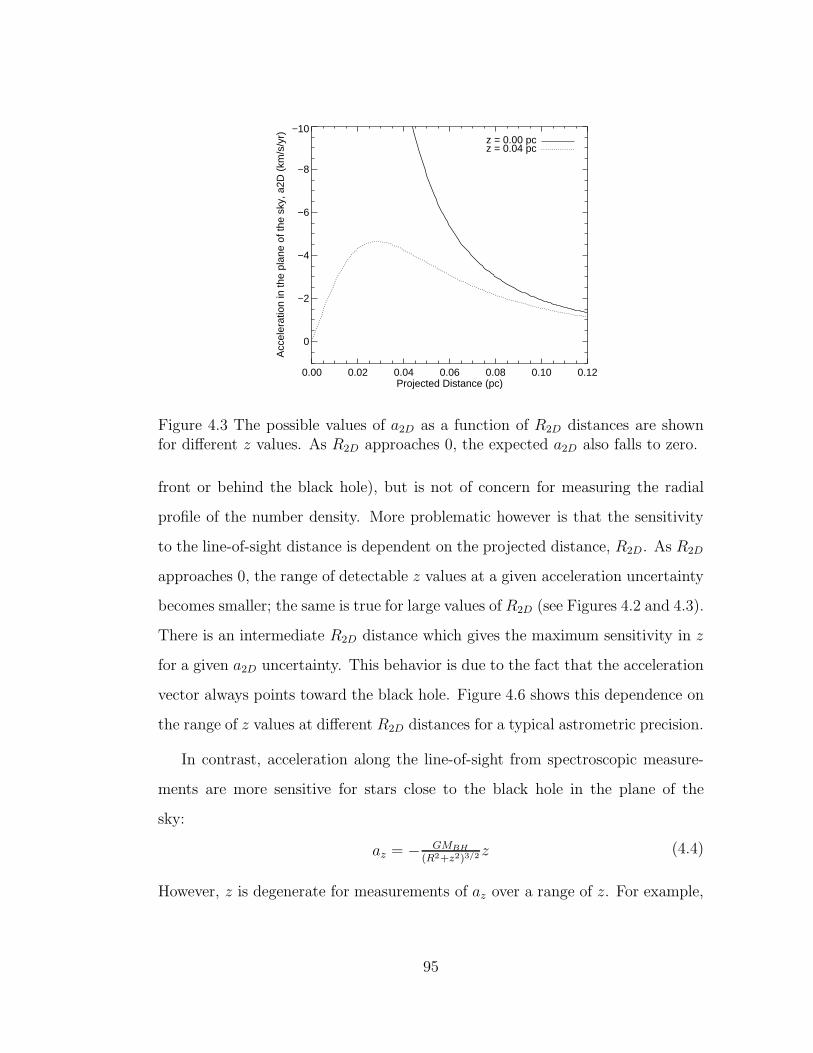
0.00 0.02 0.04 0.06 0.08 0.10 0.12Projected Distance (pc)

0

−2

−4

−6

−8

−10

Acc

eler

atio

n in

the

plan

e of

the

sky,

a2D

(km

/s/y

r) z = 0.00 pcz = 0.04 pc

Figure 4.3 The possible values of a2D as a function of R2D distances are shownfor different z values. As R2D approaches 0, the expected a2D also falls to zero.

front or behind the black hole), but is not of concern for measuring the radial

profile of the number density. More problematic however is that the sensitivity

to the line-of-sight distance is dependent on the projected distance, R2D. As R2D

approaches 0, the range of detectable z values at a given acceleration uncertainty

becomes smaller; the same is true for large values of R2D (see Figures 4.2 and 4.3).

There is an intermediate R2D distance which gives the maximum sensitivity in z

for a given a2D uncertainty. This behavior is due to the fact that the acceleration

vector always points toward the black hole. Figure 4.6 shows this dependence on

the range of z values at different R2D distances for a typical astrometric precision.

In contrast, acceleration along the line-of-sight from spectroscopic measure-

ments are more sensitive for stars close to the black hole in the plane of the

sky:

az = − GMBH

(R2+z2)3/2 z (4.4)

However, z is degenerate for measurements of az over a range of z. For example,

95

−0.10 −0.05 0.00 0.05 0.10Line of Sight Distance z (pc)

−60

−40

−20

0

20

40

60

Line

of S

ight

Acc

eler

atio

n (k

m/s

/yr)

R2D = 0.004 pcR2D = 0.020 pcR2D = 0.040 pc

Figure 4.4 The possible values of az as a function of z distances are shown fordifferent projected distance R2d. For a given az measurement, there is usually adegeneracy in z distance that must be broken by using limits from a2D.

0.00 0.02 0.04 0.06 0.08 0.10 0.12Projected Distance (pc)

0

10

20

30

40

50

Line

of S

ight

Acc

eler

atio

n, a

z (k

m/s

/yr)

z = 0.02 pcz = 0.04 pcz = 0.08 pc

Figure 4.5 The possible values of az as a function of R2D distances are shown fordifferent line-of-sight distances z.

96

if az is small, z can be very close to zero, or z can be very large (see Figures

4.4 and 4.5). Limits on a2D are required to break this degeneracy. Figure 4.6

summarizes our sensitivity to z given our average acceleration uncertainties in az

(9 km/s/yr at 3σ) and a2D (0.051 mas/yr/yr at 3σ). These az measurements are

based radial velocity measurements from 2006 and 2008, measured using a cross

correlation with a template M3III spectrum from the spectral templates from the

IRTF (Rayner et al., 2009). We include measurements of stars with continuum

SNR > 35, which have velocity errors of about 4 km/s. However, in order to

obtain robust acceleration measurements, an additional third epoch is required

(measurements from 2009 suffered from calibration problems, which have only

recently been resolved). The 3 σ acceleration error in the plane of the sky (a2D)

are from values reported in Yelda et al. (2010).

Presently, we should be able to detect all stars within 0.045 pc (∼ 1.12′′) in

volume around Sgr A*. Beyond this volume, we have some sensitivity out to ∼0.1 pc (2.5′′). Currently, because we have a longer time baseline of astrometric

measurements compared to radial velocities, the z distances of stars are better

constrained with a2D than with az in the survey region. Acceleration errors should

improve in the future with more temporal coverage; by 2014 (5 more years of data

beyond the data in this thesis), we predict that we will be able to obtain three

dimensional distances out to 0.12 pc (∼ 2.88′′) from Sgr A*. Further details on

the measurements and the three dimensional profile of the cluster will be given

in Do et al. (in prep).

4.4 Using velocity distributions

Accelerations could eventually provide unambiguous z distances for the stars, but

the distribution of stellar velocities can also be used as an additional constraint

97

0.00 0.02 0.04 0.06 0.08 0.10 0.12 0.14Projected Distance R2D (pc)

0.00

0.02

0.04

0.06

0.08

0.10

0.12

0.14

Line

of S

ight

Dis

tanc

e z

(pc)

2008

2010

2012

2014

a2d sensitivityaz sensitivity

Figure 4.6 The shaded regions correspond to the locations where the typicalacceleration uncertainties allow for a significant measurement of z from eitherthe line-of-sight acceleration (az, solid lines), or acceleration in the plane of thesky (a2D, dashed). The plot assumes a 3σ error of az = 9 km/s/s and a2D = 0.051mas/yr/yr. The red lines show the volume of complete coverage in z, from eitheraz or a2D, if observations were continued with the same cadence in the future.

98

to the spatial density profile. Unlike limits on z from acceleration, which depends

only on the assumed gravitational potential, the velocity distribution is dependent

on the distribution function, which describes the probability of finding a star

in a particular position in phase space. The distribution function f(xxx,vvv, t) is

a function of position, velocity and time, and fully describes the behavior of a

stellar system. With some assumptions about the stellar system, we can compare

predictions from the distribution function to observable parameters such as the

projected density profile and the velocity distributions.

In order to compare to the velocity distribution from observations, we will

make several assumptions: (1) the distribution function is time independent; (2)

the potential is Keplerian, with Ψ(r) = GM/r, which is a reasonable approxi-

mation given that we are interested in the region within ∼ 0.16 pc in projected

distance from the black hole, well inside its sphere of influence; (3) the cluster

is spherically symmetric; and (4) the distribution function is isotropic. These

assumptions result in a distribution function that is dependent only on the total

energy per unit mass, ε = Ψ− 12v2 (here, we use the same convention as Binney &

Tremaine (2008) of positive ε for bound stars). With the assumption of spherical

symmetry and isotropy, it is possible to uniquely invert a given spatial density

profile, ν(r) (and through a change of variable, cast as ν(Ψ)), into a distribution

function through the Eddington formula (Binney & Tremaine, 2008):

f(ε) =1√8π2

d

dε

∫ ε

0

dΨ√ε − Ψ

dν

dΨ. (4.5)

While this inversion is possible, it is simpler to construct a distribution function

that is consistent with the observed limits on the slope of the density profile and

use the velocity distribution to check the validity of the distribution function. We

start by working through some simple models before constructing the distribution

99

function for an isotropic core.

4.4.1 The Plummer model

The Plummer model is a simple star cluster model that has analytical solutions

for a number of dynamical properties, so it is a good choice to illustrate the

effect on the velocity distribution from a density profile. The Plummer model

potential is a modified Keplerian potential with a softening factor, b, to prevent

the potential approaching infinity at the center of the cluster:

Ψ =GM

(r2 + b2)1/2(4.6)

The distribution function of the Plummer model is a special form of the more

general distribution function that depends only on a power law of the total energy,

ε = Ψ− 12v2, where Ψ is the potential, and v is the total velocity (note that ε > 0

for bound orbits):

f(ε) =

Cεn−3/2 : ε > 0

0 : ε ≤ 0(4.7)

with n = 5 for the Plummer model. The density profile ν at radii where Ψ > 0

can be found by integrating the distribution function over all velocities:

ν(xxx) =

∫

d3vvvf(xxx,vvv) (4.8)

ν(r) = 4π

∫

√2Ψ

0

dvv2f(Ψ − 1

2v2) (4.9)

= 4πC

∫

√2Ψ

0

dvv2(Ψ − 1

2v2)n−3/2 (4.10)

100

The limits of the integral range between zero and the escape velocity at r. This

equation can be simplified by using the trigonometric substitution v2 = 2Ψ cos2 θ.

The solution becomes:

ν = cnΨn, for Ψ > 0, where cn =

(2π)3/2(n − 32)!C

n!(4.11)

for cn to be finite, n > 1/2. For the Plummer model, ν(r) ∝ 1/(r2 + b2)5/2. With

the distribution function and the potential, the velocity distribution as well as

its moments can be computed. The probability density of total velocities at a

projected distance R from the black hole can be computed by integrating along

the line-of-sight:

F (R, v) =

∫

dzf(xxx,vvv)∫

dzd3vvvf(xxx,vvv)(4.12)

=

∫

rdr√r2 − R2

f(ε)

Σ(R)(4.13)

Σ(R)F (R, v) =

∫

q

4

v4−1

0

rdr√r2 − R2

(Ψ(r) − 1

2v2)7/2 (4.14)

with the substitution dz = rdr/√

r2 − R2 and the projected density profile:

Σ(R) =

∫

dzd3vvvf(xxx,vvv) =

∫ ∞

R

rdr√r2 − R2

ν(r) (4.15)

=

∫ ∞

R

rdr√r2 − R2

Ψ(r)5 ∝ 1

(1 + R2)2.

Figure 4.7 shows a plot of F (R, v) for the center of the cluster as well as a

scaled projected radius R = 2. Note that the width of the distribution is smaller

at R = 2, consistent with being further from the center of the potential.

The line-of-sight velocity distribution, vz, can be computed by integrating over

101

0.0 0.5 1.0 1.5 2.0v

0.00

0.01

0.02

0.03

0.04

0.05

F(R

,v) R = 0

R = 2

Figure 4.7 F (R, v) for the Plummer Model at the center of the cluster (R=0,solid) and at a dimensionless projected distance of 2 (twice the value of b = 1 inthis case).

−1.0 −0.5 0.0 0.5 1.0vz

0.00

0.01

0.02

0.03

0.04

0.05

F(R

,vz)

R = 0

R = 2

Figure 4.8 Velocity profile along the line-of-sight, F (R, vz), for the PlummerModel at the center of the cluster (R=0, solid) and at a dimensionless projecteddistance of 2 (twice the value of b = 1 in this case).

102

the plane-of-sky velocity components – vR, the velocity in the radial direction,

and vT , the transverse velocity in the plane of the sky:

F (R, vz)dvz =

∫

dz

∫

d2v⊥f(ε) (4.16)

=

∫

rdr√r2 − R2

∫

dvT dvRf(Ψ − 1

2v2)

=

∫

rdr√r2 − R2

∫ vTMax

0

dvT

∫ vRMax

0

dvR(Ψ − 1

2(v2

R + v2T + v2

z))7/2

=π

144√

2

∫

√2Ψ(r)

0

rdr√r2 − R2

(2Ψ(r) − v2z)

9/2,

where vRMax =√

2Ψ − v2z − v2

T and vTMax =√

2Ψ − v2z . Figure 4.8 shows the

probability density F (R, vz).

The velocity distribution require numerical integration to derive the profile,

however, the moments of the velocity, such as the mean and variance, are ana-

lytical:

vvv(r) =1

ν(r)

∫

d3vvvvvvf(Ψ − 1

2v2) = 0 (4.17)

σ2(r) =1

ν(r)

∫

d3vvv(v − v)2f(Ψ − 1

2v2) (4.18)

σ2(r) ∝ 1√1 + r2

(4.19)

4.4.2 Power law density profiles

The Plummer model is a self-consistent model where the potential is generated by

the tracer population (stars) such that, with Poisson’s equation (∇2Ψ = 4πGρ),

the density ρ(r) corresponds to the Plummer potential. This self-consistency

is not necessarily required to compute the distribution function if we know the

103

0.0 0.5 1.0 1.5 2.0v

0.00

0.01

0.02

0.03

0.04

0.05

F(R

,v)

v2 dv

R = 0

R = 2

0.0 0.5 1.0 1.5v

0.0

0.2

0.4

0.6

0.8

1.0

CD

F

Figure 4.9 Left: The probability that a star is observed with a velocity between vand v+dv for the Plummer model. Right: The probability that a star is observedwith a velocity less than v.

potential and the density profile. For an isotropic, spherically symmetric system,

a density profile can be inverted with knowledge of the potential to obtain a

unique distribution function through Equation 4.5. For power a law number

density profile, ν(r), with a power law slope γ in a Keplerian potential Ψ = GM/r:

ν(r) = νor−γ, (4.20)

the corresponding distribution function is:

f(ε) = εγ− 3

2 (4.21)

Using γ = 7/4, the Bahcall-Wolf cusp slope, as an example, we can derive the

expected velocity distributions using the same procedures as for the Plummer

104

model:

f(ε) = ε1/4 (4.22)

Σ(R)F (R, v) =

∫

dzf(ε) =

∫ 2/v2

R

rdr√r2 − R2

(1

r− 1

2v2)1/4 (4.23)

where we have substituted Ψ = 1/r and with the surface density profile:

Σ(R) =

∫ ∞

R

rdr√r2 − R2

ν(r) (4.24)

=

∫ ∞

R

rdr√r2 − R2

r−7/4 = −4πΓ(3/8)

Γ(−1/8)R−3/4 (4.25)

The integral for Σ(r)F (R, v) diverges when v = 0, but this is not a problem as

there is negligible phase space available at v = 0. This can be seen when we

compute, P (< v) the probability that a star is found with velocity less than v:

P (R, < v) =

∫ v

0

F (R, v)d3vvv = 4π

∫ v

0

v2dvF (R, v) (4.26)

Both P (R, < v) and the integrand are plotted in Figure 4.9 and Figure 4.10 for

the Plummer model and the cusp model, respectively. P (R, < v) is essentially

the cumulative distribution function for the total velocity, and can be used to

compare directly with the observations. Furthermore, since we assumed spherical

symmetry in the system, we can compare the velocity distributions taken in annuli

around the cluster center:

P (R1 < R < R2, < v) = 2π

∫ R2

R1

RdR

∫ v

0

v2dvF (R, v) (4.27)

105

0 1 2 3 4 5v

0.001

0.010

0.100

F(R

,v)

v2 dv

R = 0.1R = 0.5R = 2.0

0 1 2 3 4 5v

0.0

0.2

0.4

0.6

0.8

1.0

CD

F

Figure 4.10 Left: The probability that a star is observed with a velocity betweenv and v + dv for the Bahcall and Wolf stellar cusp model with γ = 7/4. Right:The probability that a star is observed with a velocity less than v.

4.4.3 An isotropic core model

Based on the limits set by the surface density profile of stars in the Galactic

center, the Bahcall and Wolf cusp of γ = 7/4 is ruled out, so we need to find a

distribution function that will produce a flatter core. Since we are working with

distribution functions that only depend on energy, we can try a model where

certain energies are excluded. Following Merritt (2010), we will remove the most

bound stars from the star cluster by introducing an energy cutoff in the power-law

form of f(ε):

f(ε) =

εγ−3/2 : ε > 0

0 : ε ≤ 0

0 : ε ≥ Eb

(4.28)

where, Eb is the binding energy at the radius rb, such that Eb = Ψb. For the

purpose of this model, we will set γ = 7/4, which is very close to the value of

γ = 1.8 found from number counts outside the region where the density profile

106

0.001 0.010 0.100 1.000 10.000Energy

0.1

1.0

10.0

f(E

)(Ψ

− E

)−1/

2

Eb

0.01 0.10 1.00 10.00r

0.01

0.10

1.00

10.00

100.00

Spa

ce D

ensi

ty

Core Modelr−1/2

r−7/4

Figure 4.11 Left: The integrand for ν(r) showing the energy cutoff at εb. Right:The resulting density profile is more shallow than the Bahcall and Wolf solutionat r < rb, and is within the range allowed by observations.

is flat (Schodel et al., 2007). At r ≥ rb, the spatial density profile is as before,

ν(r) ∝ r7/4. For r < rb:

ν(r) = 4π

∫

f(ε)v2dv (4.29)

= 4π

∫ Ψb

0

√

2(Ψ − ε)f(ε)dε (4.30)

The full density profile can be computed through numerical integration (see Fig-

ure 4.11). For r ≪ rb, the density approaches ν(r) ∝ r−1/2, which indicates that

removing highly bound stars has flatten the number density profile, but has not

removed all stars or created a central minimum.

Similarly, we can compute F (R, v) and P (R, < v) using the Keplerian poten-

tial Ψ(r) = GM/r:

F (R, v) =

∫ rmax

rmin

rdr√r2 − R2

f(Ψ(r) − 1

2v2) (4.31)

107

0 1 2 3 4 5v

0.001

0.010

0.100

F(R

,v)

v2 dv

R = 0.1R = 0.5R = 2.0

0 1 2 3 4 5v

0.0

0.2

0.4

0.6

0.8

1.0

CD

F

Figure 4.12 Left: The probability that a star is observed with a velocity betweenv and v + dv for the isotropic core model. Note that beyond Rb = 1.0, theprobability density is identical to the cusp model in Figure 4.10. Right: Theprobability that a star is observed with a velocity less than v.

where rmin = min(R, 11/rb+v2/2

) and rmax = 2/v2. There is a minimum radius

for each velocity because we removed the most bound stars. This also indicates

why there are stars in the region r < rb, since the distribution has a cutoff

only in energy. Both F (R, v) and P (R, < v) must be computed numerically.

Their distributions are shown in Figure 4.12. These probability distributions

for velocities have a very different shape than the purely power law model in

Figure 4.10 for R < rb due to the removal of a range of possible velocities. This

comparison indicates that there are notable differences in the shape and mean of

the distribution of total velocities as a function of R between models with different

density profiles. We note that none of these velocity distributions correspond to

a Maxwell-Boltzmann distribution despite the fact that the models are isotropic.

108

4.4.4 Beyond isotropic models

Because isotropic models with power law density profiles cannot have a power

law slope γ < 1/2 (An & Evans, 2006), we would need to construct anisotropic

distribution functions in order to create the presence of a ‘hole’ in the stellar

density profile. For a spherically symmetric system, anisotropy can be included

in the distribution function by the inclusion of the angular momentum, L. The

inclusion of angular momentum means that there is no longer a unique inversion

between ν(r) and f(ε, L). Computing the velocity distribution of anisotropic core

models is out of the scope of this thesis, but we will briefly describe a method

suggested by Merritt (2010); the distribution function of the isotropic core model

can be modified to include an angular momentum, J , cutoff: f(ε, L) = 0 for

J ≤ Jb. This model would remove all stars that come within rb of the black hole,

clearing out the central region of the cluster.

4.5 Conclusion

We have shown that the addition of kinematic information should improve the

constraints on the true distribution of stars in the region around Sgr A*. For

stars with significant acceleration detections, we will be able to constrain their

distribution directly. In addition, the three-dimensional velocity measurements of

all stars should help us constrain the distribution function of the cluster. We have

shown that the predicted velocity distributions are distinctive enough that com-

parisons with data should rule out certain distribution functions. Some challenges

in these comparisons to observations may arise from the assumptions placed on

the models. For example, the use of a Keplerian potential is only valid within

the sphere of influence of the black hole (rs ≈ 1 pc for Sgr A*). While the stars

109

observed in this thesis are well within rs in the plane of the sky, if a large number

of stars have z distances greater than rs, then the stellar mass distribution will

be important to consider in the models. Ultimately, if we can observationally dif-

ferentiate between the possible physical scenarios that result in a flattened core

(details in Chapter 3), we will learn a great deal about the dynamical history of

the environment around a massive black hole.

110

CHAPTER 5

Conclusions

The advent of laser guide star adaptive optics has rapidly increased our under-

standing of the environment around a supermassive black hole. It is now possible

to study the physical properties of the black hole and its associated accretion

flow through its variability in the infrared. Using multiple observations and ap-

plying a statistical analysis of the data, we have been able to set new limits on

the presence of periodic phenomena responsible for its infrared variability. In

particular, it appears unlikely that the large amplitude variability is caused by

hot spots of plasma orbiting at the last stable orbit around the black hole; the

‘flickering’ is much more consistent with the variability observed at the centers

of active galaxies, which suggests that some of the same physical processes are

occurring in the accretion flow of Sgr A* though on a much smaller scale.

LGS AO has also allowed high angular resolution integral field spectroscopy of

this region, resulting in the most detailed population census performed within ∼0.16 pc of a supermassive black hole. For the first time, we are able to investigate

the predictions of a stellar cusp around massive black holes; contrary to these

predictions, we find that the old stars have a flat surface density profile close

to the black hole. The physical explanation for this puzzling result will affect

theories on the growth of the supermassive black hole as well as on the dynamical

evolution of other objects in this region.

111

5.1 Prospects for clarifying the nature of Sgr A*-IR

While we have shown that the near-IR light curves from Sgr A* are consistent

with red noise, it is difficult at this time to determine its precise physical origins.

The behavior of the Sgr A* light curves are very similar to those seen in AGNs,

whose variability has been suggested to arise from instabilities in the accretion

flow to changes in the accretion rate. Recently, further evidence of the link

between the Sgr A*-IR variability and AGNs was found with the observation of

a break frequency in the power law spectrum of Sgr A*. Using near-IR light

curves observed from Sgr A* on a scale of minutes up to years apart, Meyer

et al. (2009) found a break frequency at 154+124−87 minutes, consistent with the

relationship between the break frequency of the power spectrum and black hole

mass for AGNs observed at X-ray wavelengths (McHardy et al., 2006).

Further insights into the nature of accretion onto Sgr A* can be gained using

our current technology with observations of: (1) light curves at faster time sam-

pling, (2) the properties of the faint states of Sgr A*, and (3) the time dependent

polarization. The study of Sgr A* at fast time sampling will provide us a unique

window into the properties of accretion flow around black holes. While we have

been able to constrain the the break frequency of Sgr A* at low frequencies, we

have not observed a corresponding break at high frequencies, which may indicate

the size scale of structures in the accretion flow. The power spectra of the light

curves appear to have a consistent power law slope down to a time scale of ∼ 3

min, where the dithering pattern in our data causes a large artifact. To better

sample the fast time scales, we can use NIRC2 in its subarray mode to achieve a

cadence of 20 s, which corresponds a light travel time of only 0.5 Schwarzschild

radii, given the mass of Sgr A*. In this way, we can achieve Nyquist sampling

of structures on the order of a Schwarzschild radius. In comparison, the fastest

112

timescale probed so far for any black hole is on the order of milliseconds for

X-ray binaries (Gierlinski & Zdziarski, 2003), which corresponds to about 10-20

Schwarzschild radii for a stellar mass black hole. In addition, the nature of the

faint state of Sgr A* is important to establish whether there is a distinct quiescent

state of Sgr A* and to measure the fraction of light produced by faint unresolved

stars as opposed to accretion onto the black hole. Polarization will also offer a

new window onto the physics of the accretion flow, and has been suggested to

show stronger periodic behavior than the total intensity (e.g. Zamaninasab et al.,

2010).

5.2 Origin of the missing stellar cusp

Given the current limits on the stellar density at the Galactic center, we can

rule out the density profile in the equilibrium solution from Bahcall & Wolf

(1977) for the tracer population of red giants. It is crucial to understand the

tracer population as well as the dynamics in this region to properly interpret

this result. In principle, the red giants should have had > 1 Gyr to achieve a

dynamically relaxed state and should be a good tracer of the underlying stellar

distribution. However, since the nuclear star cluster is not an isolated system,

dynamical interactions involving objects such as an intermediate mass black hole

would change the distribution of stars. In addition, the larger physical size of

the red giants compared to main sequence stars may be a factor in increasing the

frequency of collisions as well as increasing their cross section for tidal disruption

by Sgr A*. More theoretical work with simulations will be required to produce

testable predictions of the current configuration of stars in order to compare to

observations. In terms of observations, the most important task will be to break

the degeneracy in the surface density profile to determine if the volume density

113

is flat or falls in the core. Kinematic measurements as well as extending the

radial coverage beyond the current survey should greatly reduce this degeneracy.

Finally, the effect of the size of the red giants can be tested with better spectral

typing to determine if there is a difference in the density profiles of giants of

different sizes.

114

APPENDIX A

OSIRIS wavelength calibrations

Every spectrograph requires wavelength calibration in order to transform flux

measurement at each pixel of the detector into flux as a function of wavelength.

OSIRIS, being an integral field spectrograph, simultaneously measures a spec-

trum at every spatial pixel location for up to ∼ 3000 spectra, all of which must be

calibrated. The initial calibration is achieved using an arc lamp at the telescope

that scans across all the lenslets (see the OSIRIS User Manual). This calibration

is done by the instrument team when major changes to the instrument occur,

and is built into the data reduction pipeline.

In 2007, it was discovered that the spectra from different spatial locations in

an OSIRIS cube were offset by an average of about 0.1 spectral channel, with

maximum offsets up to 0.5 spectral channels on the edges of the Kn3 filter (each

spectral channel is 2.5 A). In the following sections I describe the diagnostics of

these wavelength shifts as well as the subsequent correction and stability of the

wavelength solution.

A.1 Characterizing the wavelength shifts

The wavelength shifts between different spatial pixels were determined using sky

observations. The near-infrared sky has strong OH emission lines, which can be

used to test the absolute wavelength calibration (the conversion into A) as well

115

as relative offsets between spectra at different spatial locations. Of the OH lines

observable in the Kn3 filter (λ = 2.121− 2.229 µm), there are 5 strong lines that

are not blended with neighboring lines (see Table A.1). In order to determine

the effectiveness of the wavelength calibration, I fitted the centroids of these lines

with a Gaussian in the spectrum for each spatial pixel in the data cube. Each

spectrum was extracted as the median of the neighboring 3 × 3 spatial pixel at

each wavelength channel in order to avoid cosmic rays and bad pixels. I then

used the mean difference between the measured wavelengths of the centroids and

its corresponding vacuum wavelength to be the average wavelength shift for that

spatial pixel. In order to determine whether there is a wavelength dependence to

the OH line offsets, I also performed a linear fit to the wavelength difference as a

function of wavelength. I find that the linear fit is flat, and not significantly better

than using a constant mean to describe the wavelength offsets from vacuum in

the Kn3 wavelength range. The mean wavelength offset range from -0.22 A(3

km/s at 2.1661 µm), with a σ = 0.08 A in 2006 to −0.41 A(5.7 km/s at 2.1661

µm) with σ = 0.09 A in 2008.

Table A.1 OH lines used for refining the wavelength calibration in the Kn3 filter

OH Line (A)21507.321537.621802.221955.622125.5

In addition to using the OH lines as tests of the absolute wavelength calibra-

tion, I also measured the relative wavelength solution between each lenslet. The-

oretically, after wavelength calibration, the spectrum from every lenslet should

have been interpolated onto the same wavelength at each spectral channel. Hav-

116

ing all the spectra with flux correctly assigned to the same grid of spectral chan-

nels is essential to be able to combine the flux from different spatial locations to

establish higher signal to noise spectra. Mismatches in the relative wavelength

calibration between spaxels can lead to incorrectly measured line widths and cen-

troids when using extraction apertures greater than 1 spaxel in size. In addition,

a large offset in the wavelength solution between each lenslet will lead to very

poor sky subtraction if the sky is obtained at a different lenslet location, such

as for the Galactic center observations. Sufficiently mismatched spectra are ap-

parent in the residual from subtracting skies from two different spatial locations,

resulting in small P-Cygni profiles from shifted OH lines.

In order to establish the relative shifts between the spectra from each lenslet,

I cross-correlated each spectrum with the one extracted from the central lenslet.

In order to avoid bad pixels, the spectrum from each lenslet is the median of a

3x3 box centered on the lenslet of interest (within a 3x3 box, the relative shifts

between the spectra do not appear significant).

117

060701 Kn3 35 mas Rel.

0 10 20 30 40 50Mean: 0.02 sigma: 0.02

0

10

20

30

40

50

60

pix

−0.3

−0.2

−0.1

0.0

0.1

0.2

0.3060701 Kn3 35 mas Abs

0 10 20 30 40 50Mean: −0.19 sigma: 0.08

0

10

20

30

40

50

60

Ang

−3.0

−2.0

−1.0

0.0

1.0

2.0

3.0070718 Kn3 35 mas Rel.

0 10 20 30 40 50Mean: 0.02 sigma: 0.04

0

10

20

30

40

50

60

pix

−0.3

−0.2

−0.1

0.0

0.1

0.2

0.3070718 Kn3 35 mas Abs

0 10 20 30 40 50Mean: 0.09 sigma: 0.14

0

10

20

30

40

50

60

Ang

−3.0

−2.0

−1.0

0.0

1.0

2.0

3.0

080516 Kn3 35 mas Rel.

0 10 20 30 40 50Mean: 0.04 sigma: 0.03

0

10

20

30

40

50

60

pix

−0.3

−0.2

−0.1

0.0

0.1

0.2

0.3080516 Kn3 35 mas Abs

0 10 20 30 40 50Mean: −0.36 sigma: 0.11

0

10

20

30

40

50

60

Ang

−3.0

−2.0

−1.0

0.0

1.0

2.0

3.0090507 Kn3 35 mas Rel.

0 10 20 30 40 50Mean: 0.02 sigma: 0.04

0

10

20

30

40

50

60

pix

−0.3

−0.2

−0.1

0.0

0.1

0.2

0.3090507 Kn3 35 mas Abs

0 10 20 30 40 50Mean: −2.17 sigma: 0.13

0

10

20

30

40

50

60

Ang

−3.0

−2.0

−1.0

0.0

1.0

2.0

3.0

Figure A.1 Both relative and absolute wavelength shifts as measured from theOH lines from 2006-2009. Note that in 2009, the wavelength solution is shiftedby about 2 A compared to previous years due to thermal problems with thespectrograph.

118

APPENDIX B

Catalog of OSIRIS spectra

Figure B.1 shows the compilation of spectra that were spectral-typed as young

based on the presence of Br gamma in the Kn3 wavelength range, while Figure

B.11 shows early-type spectra without Br gamma absorption lines. Figure B.15

shows the spectral of all identified late-type stars. These spectra were extracted

using the standard 2 pixel radius aperture, with sky subtraction from the median

of an annulus starting at 2 pixels out to 4 pixels. These spectra have also been

corrected for telluric features and smoothed using a 3 pixel box-car convolution,

and are grouped by OSIRIS field locations. More information about each of the

spectra can be found in Tables 3.2 and 3.3. Spectra of the IRS16 sources have not

been included due to difficulties in determining the radial velocity of the Wolf-

Rayet stars (the hydrogen emission lines from the stellar winds obscures the true

radial velocity of the spectra).

119

2.14 2.16 2.18 2.20 2.220.6

0.8

1.0

1.2

S0−2, C, Kp = 14.1

2.14 2.16 2.18 2.20 2.220.6

0.8

1.0

1.2

S0−15, C, Kp = 13.7

2.14 2.16 2.18 2.20 2.220.6

0.8

1.0

1.2

S1−8, C, Kp = 14.2

2.14 2.16 2.18 2.20 2.220.6

0.8

1.0

1.2

S0−4, C, Kp = 14.5

2.14 2.16 2.18 2.20 2.220.6

0.8

1.0

1.2

S0−19, C, Kp = 15.5

Na

IN

a I

Br

γ

Ti I

Si I

Ti I

He

II

Figure B.1 Early-type stars with Br gamma lines in Kn3, shifted to rest wave-length and grouped by OSIRIS field location.

120

2.14 2.16 2.18 2.20 2.220.6

0.8

1.0

1.2

S0−7, C, Kp = 15.5

2.14 2.16 2.18 2.20 2.220.6

0.8

1.0

1.2

S0−20, C, Kp = 15.9

2.14 2.16 2.18 2.20 2.220.6

0.8

1.0

1.2

S0−30, C, Kp = 16.1

2.14 2.16 2.18 2.20 2.220.6

0.8

1.0

1.2

S1−12, C, Kp = 13.8

2.14 2.16 2.18 2.20 2.220.6

0.8

1.0

1.2

S1−2, C, Kp = 14.9

Na

IN

a I

Br

γ

Ti I

Si I

Ti I

He

II

Figure B.2 Continuation of Figure B.1

121

2.14 2.16 2.18 2.20 2.220.6

0.8

1.0

1.2

S0−9, C, Kp = 14.4

2.14 2.16 2.18 2.20 2.220.6

0.8

1.0

1.2

S0−3, C, Kp = 14.5

2.14 2.16 2.18 2.20 2.220.6

0.8

1.0

1.2

S1−33, C, Kp = 15.0

2.14 2.16 2.18 2.20 2.220.6

0.8

1.0

1.2

S0−31, C, Kp = 15.1

2.14 2.16 2.18 2.20 2.220.6

0.8

1.0

1.2

S0−5, C, Kp = 15.1

Na

IN

a I

Br

γ

Ti I

Si I

Ti I

He

II


122

2.14 2.16 2.18 2.20 2.220.6

0.8

1.0

1.2

S0−11, C, Kp = 15.3

2.14 2.16 2.18 2.20 2.220.6

0.8

1.0

1.2

S0−8, C, Kp = 15.8

2.14 2.16 2.18 2.20 2.220.6

0.8

1.0

1.2

S0−14, C, Kp = 13.7

2.14 2.16 2.18 2.20 2.220.6

0.8

1.0

1.2

S0−1, C, Kp = 14.7

2.14 2.16 2.18 2.20 2.220.6

0.8

1.0

1.2

S1−22, C, Kp = 12.7

Na

IN

a I

Br

γ

Ti I

Si I

Ti I

He

II


123

2.14 2.16 2.18 2.20 2.220.6

0.8

1.0

1.2

S1−14, C, Kp = 12.8

2.14 2.16 2.18 2.20 2.220.6

0.8

1.0

1.2

S1−1, C, Kp = 13.1

2.14 2.16 2.18 2.20 2.220.6

0.8

1.0

1.2

S2−58, E, Kp = 14.1

2.14 2.16 2.18 2.20 2.220.6

0.8

1.0

1.2

S3−3, E, Kp = 15.1

2.14 2.16 2.18 2.20 2.220.6

0.8

1.0

1.2

S2−61, E, Kp = 15.5

Na

IN

a I

Br

γ

Ti I

Si I

Ti I

He

II


124

2.14 2.16 2.18 2.20 2.220.6

0.8

1.0

1.2

S2−64, E, Kp = 15.8

2.14 2.16 2.18 2.20 2.220.6

0.8

1.0

1.2

S3−34, E, Kp = 13.5

2.14 2.16 2.18 2.20 2.220.6

0.8

1.0

1.2

S3−314, E, Kp = 15.4

2.14 2.16 2.18 2.20 2.220.6

0.8

1.0

1.2

S2−22, E, Kp = 12.9

2.14 2.16 2.18 2.20 2.220.6

0.8

1.0

1.2

S2−19, N, Kp = 12.6

Na

IN

a I

Br

γ

Ti I

Si I

Ti I

He

II


125

2.14 2.16 2.18 2.20 2.220.6

0.8

1.0

1.2

S2−76, N, Kp = 15.2

2.14 2.16 2.18 2.20 2.220.6

0.8

1.0

1.2

S1−18, N, Kp = 15.0

2.14 2.16 2.18 2.20 2.220.6

0.8

1.0

1.2

S3−2, NE, Kp = 12.1

2.14 2.16 2.18 2.20 2.220.6

0.8

1.0

1.2

irs33N, S, Kp = 11.4

2.14 2.16 2.18 2.20 2.220.6

0.8

1.0

1.2

S2−21, S, Kp = 13.5

Na

IN

a I

Br

γ

Ti I

Si I

Ti I

He

II


126

2.14 2.16 2.18 2.20 2.220.6

0.8

1.0

1.2

S1−19, S, Kp = 13.8

2.14 2.16 2.18 2.20 2.220.6

0.8

1.0

1.2

S2−77, S, Kp = 13.8

2.14 2.16 2.18 2.20 2.220.6

0.8

1.0

1.2

S2−317, S, Kp = 15.6

2.14 2.16 2.18 2.20 2.220.6

0.8

1.0

1.2

S2−55, SE, Kp = 15.4

2.14 2.16 2.18 2.20 2.220.6

0.8

1.0

1.2

S2−50, SE, Kp = 15.5

Na

IN

a I

Br

γ

Ti I

Si I

Ti I

He

II


127

2.14 2.16 2.18 2.20 2.220.6

0.8

1.0

1.2

S2−59, SE, Kp = 15.4

2.14 2.16 2.18 2.20 2.220.6

0.8

1.0

1.2

S1−24, SE, Kp = 11.6

2.14 2.16 2.18 2.20 2.220.6

0.8

1.0

1.2

S2−4, SE, Kp = 12.3

2.14 2.16 2.18 2.20 2.220.6

0.8

1.0

1.2

S2−6, SE, Kp = 12.0

2.14 2.16 2.18 2.20 2.220.6

0.8

1.0

1.2

S2−17, SE, Kp = 10.9

Na

IN

a I

Br

γ

Ti I

Si I

Ti I

He

II


128

2.14 2.16 2.18 2.20 2.220.6

0.8

1.0

1.2

S3−30, SE, Kp = 12.8

2.14 2.16 2.18 2.20 2.220.6

0.8

1.0

1.2

irs13E1, SW, Kp = 10.9

2.14 2.16 2.18 2.20 2.220.6

0.8

1.0

1.2

S3−190, W, Kp = 14.1


129

2.14 2.16 2.18 2.20 2.220.6

0.8

1.0

1.2

S1−4, C, Kp = 12.6

2.14 2.16 2.18 2.20 2.220.6

0.8

1.0

1.2

S1−3, C, Kp = 12.1

2.14 2.16 2.18 2.20 2.220.6

0.8

1.0

1.2

S1−34, C, Kp = 13.2

2.14 2.16 2.18 2.20 2.220.6

0.8

1.0

1.2

S3−5, E, Kp = 12.2

2.14 2.16 2.18 2.20 2.220.6

0.8

1.0

1.2

S3−10, E, Kp = 12.4

Na

IN

a I

Br

γ

Ti I

Si I

Ti I

He

II

Figure B.11 Early-type stars with featureless spectra in Kn3, shifted to rest wave-length and grouped by OSIRIS field location.

130

2.14 2.16 2.18 2.20 2.220.6

0.8

1.0

1.2

S2−5, E, Kp = 13.3

2.14 2.16 2.18 2.20 2.220.6

0.8

1.0

1.2

S2−74, N, Kp = 13.3

2.14 2.16 2.18 2.20 2.220.6

0.8

1.0

1.2

S2−7, N, Kp = 14.1

2.14 2.16 2.18 2.20 2.220.6

0.8

1.0

1.2

irs29N, NW, Kp = 10.3

2.14 2.16 2.18 2.20 2.220.6

0.8

1.0

1.2

S2−16, NW, Kp = 11.9

Na

IN

a I

Br

γ

Ti I

Si I

Ti I

He

II

Figure B.12 Continuation of Figure B.11.

131

2.14 2.16 2.18 2.20 2.220.6

0.8

1.0

1.2

S3−17, NW, Kp = 14.1

2.14 2.16 2.18 2.20 2.220.6

0.8

1.0

1.2

S4−12, NW, Kp = 14.9

2.14 2.16 2.18 2.20 2.220.6

0.8

1.0

1.2

S3−7, SE, Kp = 13.9

2.14 2.16 2.18 2.20 2.220.6

0.8

1.0

1.2

S3−12, SE, Kp = 12.0

2.14 2.16 2.18 2.20 2.220.6

0.8

1.0

1.2

S3−96, SW, Kp = 14.5

Na

IN

a I

Br

γ

Ti I

Si I

Ti I

He

II


132

2.14 2.16 2.18 2.20 2.220.6

0.8

1.0

1.2

irs13E2, SW, Kp = 10.8

2.14 2.16 2.18 2.20 2.220.6

0.8

1.0

1.2

irs13E4, SW, Kp = 12.0

2.14 2.16 2.18 2.20 2.220.6

0.8

1.0

1.2

S1−22, SW, Kp = 12.7

2.14 2.16 2.18 2.20 2.220.6

0.8

1.0

1.2

S1−21, W, Kp = 13.3


133

2.14 2.16 2.18 2.20 2.220.6

0.8

1.0

1.2

S0−17, C, Kp = 15.7

2.14 2.16 2.18 2.20 2.220.6

0.8

1.0

1.2

S1−5, C, Kp = 12.8

2.14 2.16 2.18 2.20 2.220.6

0.8

1.0

1.2

S0−13, C, Kp = 13.5

2.14 2.16 2.18 2.20 2.220.6

0.8

1.0

1.2

S0−6, C, Kp = 14.2

2.14 2.16 2.18 2.20 2.220.6

0.8

1.0

1.2

S1−13, C, Kp = 14.2

Na

IN

a I

Br

γ

Ti I

Si I

Ti I

He

II

Figure B.15 Late-type stars in Kn3, shifted to rest wavelength and grouped byOSIRIS field location.

134

2.14 2.16 2.18 2.20 2.220.6

0.8

1.0

1.2

S1−15, C, Kp = 14.2

2.14 2.16 2.18 2.20 2.220.6

0.8

1.0

1.2

S0−12, C, Kp = 14.4

2.14 2.16 2.18 2.20 2.220.6

0.8

1.0

1.2

S1−10, C, Kp = 14.9

2.14 2.16 2.18 2.20 2.220.6

0.8

1.0

1.2

S0−28, C, Kp = 15.8

2.14 2.16 2.18 2.20 2.220.6

0.8

1.0

1.2

S1−6, C, Kp = 15.5

Na

IN

a I

Br

γ

Ti I

Si I

Ti I

He

II


135

2.14 2.16 2.18 2.20 2.220.6

0.8

1.0

1.2

S1−31, C, Kp = 15.7

2.14 2.16 2.18 2.20 2.220.6

0.8

1.0

1.2

S0−29, C, Kp = 15.6

2.14 2.16 2.18 2.20 2.220.6

0.8

1.0

1.2

S0−27, C, Kp = 15.7

2.14 2.16 2.18 2.20 2.220.6

0.8

1.0

1.2

S2−31, E, Kp = 13.1

2.14 2.16 2.18 2.20 2.220.6

0.8

1.0

1.2

S3−6, E, Kp = 12.9

Na

IN

a I

Br

γ

Ti I

Si I

Ti I

He

II


136

2.14 2.16 2.18 2.20 2.220.6

0.8

1.0

1.2

S2−11, E, Kp = 12.0

2.14 2.16 2.18 2.20 2.220.6

0.8

1.0

1.2

S4−1, E, Kp = 13.5

2.14 2.16 2.18 2.20 2.220.6

0.8

1.0

1.2

S3−8, E, Kp = 14.0

2.14 2.16 2.18 2.20 2.220.6

0.8

1.0

1.2

S2−75, E, Kp = 14.5

2.14 2.16 2.18 2.20 2.220.6

0.8

1.0

1.2

S3−36, E, Kp = 14.7

Na

IN

a I

Br

γ

Ti I

Si I

Ti I

He

II


137

2.14 2.16 2.18 2.20 2.220.6

0.8

1.0

1.2

S3−38, E, Kp = 15.0

2.14 2.16 2.18 2.20 2.220.6

0.8

1.0

1.2

S3−385, E, Kp = 15.3

2.14 2.16 2.18 2.20 2.220.6

0.8

1.0

1.2

S2−83, E, Kp = 15.6

2.14 2.16 2.18 2.20 2.220.6

0.8

1.0

1.2

S2−65, E, Kp = 15.8

2.14 2.16 2.18 2.20 2.220.6

0.8

1.0

1.2

S3−383, E, Kp = 15.4

Na

IN

a I

Br

γ

Ti I

Si I

Ti I

He

II


138

2.14 2.16 2.18 2.20 2.220.6

0.8

1.0

1.2

S2−47, E, Kp = 14.2

2.14 2.16 2.18 2.20 2.220.6

0.8

1.0

1.2

S1−25, E, Kp = 13.5

2.14 2.16 2.18 2.20 2.220.6

0.8

1.0

1.2

S1−68, E, Kp = 13.4

2.14 2.16 2.18 2.20 2.220.6

0.8

1.0

1.2

S3−16, E, Kp = 15.3

2.14 2.16 2.18 2.20 2.220.6

0.8

1.0

1.2

S2−51, N, Kp = 15.9

Na

IN

a I

Br

γ

Ti I

Si I

Ti I

He

II


139

2.14 2.16 2.18 2.20 2.220.6

0.8

1.0

1.2

S2−205, N, Kp = 15.8

2.14 2.16 2.18 2.20 2.220.6

0.8

1.0

1.2

S2−32, N, Kp = 12.4

2.14 2.16 2.18 2.20 2.220.6

0.8

1.0

1.2

S3−68, N, Kp = 15.8

2.14 2.16 2.18 2.20 2.220.6

0.8

1.0

1.2

S2−26, N, Kp = 13.7

2.14 2.16 2.18 2.20 2.220.6

0.8

1.0

1.2

S2−2, N, Kp = 14.1

Na

IN

a I

Br

γ

Ti I

Si I

Ti I

He

II


140

2.14 2.16 2.18 2.20 2.220.6

0.8

1.0

1.2

S1−44, N, Kp = 15.6

2.14 2.16 2.18 2.20 2.220.6

0.8

1.0

1.2

S2−37, N, Kp = 15.8

2.14 2.16 2.18 2.20 2.220.6

0.8

1.0

1.2

S1−20, N, Kp = 12.7

2.14 2.16 2.18 2.20 2.220.6

0.8

1.0

1.2

S3−14, N, Kp = 13.9

2.14 2.16 2.18 2.20 2.220.6

0.8

1.0

1.2

S4−2, NE, Kp = 13.0

Na

IN

a I

Br

γ

Ti I

Si I

Ti I

He

II


141

2.14 2.16 2.18 2.20 2.220.6

0.8

1.0

1.2

S3−37, NE, Kp = 15.1

2.14 2.16 2.18 2.20 2.220.6

0.8

1.0

1.2

S2−80, NE, Kp = 15.6

2.14 2.16 2.18 2.20 2.220.6

0.8

1.0

1.2

S3−39, NE, Kp = 13.6

2.14 2.16 2.18 2.20 2.220.6

0.8

1.0

1.2

S2−12, NE, Kp = 15.3

2.14 2.16 2.18 2.20 2.220.6

0.8

1.0

1.2

S2−34, NE, Kp = 15.4

Na

IN

a I

Br

γ

Ti I

Si I

Ti I

He

II


142

2.14 2.16 2.18 2.20 2.220.6

0.8

1.0

1.2

S2−23, NE, Kp = 14.8

2.14 2.16 2.18 2.20 2.220.6

0.8

1.0

1.2

S3−284, NW, Kp = 13.7

2.14 2.16 2.18 2.20 2.220.6

0.8

1.0

1.2

S2−85, NW, Kp = 12.2

2.14 2.16 2.18 2.20 2.220.6

0.8

1.0

1.2

S3−288, NW, Kp = 14.3

2.14 2.16 2.18 2.20 2.220.6

0.8

1.0

1.2

S3−149, NW, Kp = 13.3

Na

IN

a I

Br

γ

Ti I

Si I

Ti I

He

II


143

2.14 2.16 2.18 2.20 2.220.6

0.8

1.0

1.2

S4−59, NW, Kp = 13.7

2.14 2.16 2.18 2.20 2.220.6

0.8

1.0

1.2

S4−84, NW, Kp = 14.0

2.14 2.16 2.18 2.20 2.220.6

0.8

1.0

1.2

S3−262, NW, Kp = 15.1

2.14 2.16 2.18 2.20 2.220.6

0.8

1.0

1.2

S1−23, S, Kp = 11.9

2.14 2.16 2.18 2.20 2.220.6

0.8

1.0

1.2

S1−17, S, Kp = 12.5

Na

IN

a I

Br

γ

Ti I

Si I

Ti I

He

II


144

2.14 2.16 2.18 2.20 2.220.6

0.8

1.0

1.2

S2−3, S, Kp = 14.5

2.14 2.16 2.18 2.20 2.220.6

0.8

1.0

1.2

S2−57, S, Kp = 14.7

2.14 2.16 2.18 2.20 2.220.6

0.8

1.0

1.2

S2−72, S, Kp = 15.1

2.14 2.16 2.18 2.20 2.220.6

0.8

1.0

1.2

S2−49, S, Kp = 15.5

2.14 2.16 2.18 2.20 2.220.6

0.8

1.0

1.2

S1−66, S, Kp = 15.6

Na

IN

a I

Br

γ

Ti I

Si I

Ti I

He

II


145

2.14 2.16 2.18 2.20 2.220.6

0.8

1.0

1.2

S1−48, S, Kp = 15.5

2.14 2.16 2.18 2.20 2.220.6

0.8

1.0

1.2

S1−67, S, Kp = 15.6

2.14 2.16 2.18 2.20 2.220.6

0.8

1.0

1.2

S2−212, S, Kp = 15.7

2.14 2.16 2.18 2.20 2.220.6

0.8

1.0

1.2

S2−41, S, Kp = 15.5

2.14 2.16 2.18 2.20 2.220.6

0.8

1.0

1.2

S2−71, S, Kp = 15.3

Na

IN

a I

Br

γ

Ti I

Si I

Ti I

He

II


146

2.14 2.16 2.18 2.20 2.220.6

0.8

1.0

1.2

S2−62, S, Kp = 15.2

2.14 2.16 2.18 2.20 2.220.6

0.8

1.0

1.2

S1−36, S, Kp = 15.8

2.14 2.16 2.18 2.20 2.220.6

0.8

1.0

1.2

S2−308, S, Kp = 15.5

2.14 2.16 2.18 2.20 2.220.6

0.8

1.0

1.2

S1−39, S, Kp = 15.4

2.14 2.16 2.18 2.20 2.220.6

0.8

1.0

1.2

S2−134, S, Kp = 15.6

Na

IN

a I

Br

γ

Ti I

Si I

Ti I

He

II


147

2.14 2.16 2.18 2.20 2.220.6

0.8

1.0

1.2

S2−18, S, Kp = 13.3

2.14 2.16 2.18 2.20 2.220.6

0.8

1.0

1.2

S2−25, SE, Kp = 14.1

2.14 2.16 2.18 2.20 2.220.6

0.8

1.0

1.2

S3−20, SE, Kp = 14.9

2.14 2.16 2.18 2.20 2.220.6

0.8

1.0

1.2

S3−11, SE, Kp = 15.1

2.14 2.16 2.18 2.20 2.220.6

0.8

1.0

1.2

S2−73, SE, Kp = 15.2

Na

IN

a I

Br

γ

Ti I

Si I

Ti I

He

II


148

2.14 2.16 2.18 2.20 2.220.6

0.8

1.0

1.2

S3−32, SE, Kp = 15.5

2.14 2.16 2.18 2.20 2.220.6

0.8

1.0

1.2

S2−81, SE, Kp = 15.6

2.14 2.16 2.18 2.20 2.220.6

0.8

1.0

1.2

S3−151, SE, Kp = 15.7

2.14 2.16 2.18 2.20 2.220.6

0.8

1.0

1.2

S2−319, SE, Kp = 15.7

2.14 2.16 2.18 2.20 2.220.6

0.8

1.0

1.2

S3−187, SW, Kp = 14.4

Na

IN

a I

Br

γ

Ti I

Si I

Ti I

He

II


149

2.14 2.16 2.18 2.20 2.220.6

0.8

1.0

1.2

S3−291, SW, Kp = 12.2

2.14 2.16 2.18 2.20 2.220.6

0.8

1.0

1.2

S2−67, SW, Kp = 13.8

2.14 2.16 2.18 2.20 2.220.6

0.8

1.0

1.2

S2−78, SW, Kp = 13.8

2.14 2.16 2.18 2.20 2.220.6

0.8

1.0

1.2

S2−24, SW, Kp = 13.8

2.14 2.16 2.18 2.20 2.220.6

0.8

1.0

1.2

S2−70, W, Kp = 14.5

Na

IN

a I

Br

γ

Ti I

Si I

Ti I

He

II


150

2.14 2.16 2.18 2.20 2.220.6

0.8

1.0

1.2

irs29S, W, Kp = 11.3

2.14 2.16 2.18 2.20 2.220.6

0.8

1.0

1.2

S2−8, W, Kp = 12.2

2.14 2.16 2.18 2.20 2.220.6

0.8

1.0

1.2

S3−249, W, Kp = 14.7

2.14 2.16 2.18 2.20 2.220.6

0.8

1.0

1.2

S3−109, W, Kp = 15.6


151

Bibliography

Alexander, T., & Hopman, C. 2008, ArXiv e-prints

Allen, D. A., Hyland, A. R., & Hillier, D. J. 1990, MNRAS, 244, 706

An, J. H., & Evans, N. W. 2006, ApJ, 642, 752

Armitage, P. J., & Reynolds, C. S. 2003, MNRAS, 341, 1041

Aschenbach, B., Grosso, N., Porquet, D., & Predehl, P. 2004, AAP, 417, 71

Baganoff, F. K., Maeda, Y., Morris, M., Bautz, M. W., Brandt, W. N., Cui, W.,

Doty, J. P., Feigelson, E. D., Garmire, G. P., Pravdo, S. H., Ricker, G. R., &

Townsley, L. K. 2003, ApJ, 591, 891

Bahcall, J. N., & Wolf, R. A. 1976, ApJ, 209, 214

—. 1977, ApJ, 216, 883

Bailey, V. C., & Davies, M. B. 1999, MNRAS, 308, 257

Bartko, H., Martins, F., Fritz, T. K., Genzel, R., Levin, Y., Perets, H. B., Pau-

mard, T., Nayakshin, S., Gerhard, O., Alexander, T., Dodds-Eden, K., Eisen-

hauer, F., Gillessen, S., Mascetti, L., Ott, T., Perrin, G., Pfuhl, O., Reid, M. J.,

Rouan, D., Sternberg, A., & Trippe, S. 2009, ApJ, 697, 1741

Baumgardt, H., Gualandris, A., & Portegies Zwart, S. 2006, MNRAS, 372, 174

Becklin, E. E., & Neugebauer, G. 1968, ApJ, 151, 145

Belanger, G., Goldwurm, A., Melia, F., Ferrando, P., Grosso, N., Porquet, D.,

Warwick, R., & Yusef-Zadeh, F. 2005, ApJ, 635, 1095

152

Belanger, G., Terrier, R., de Jager, O. C., & Melia, F. 2008 in prep, ApJ

Benlloch, S., Wilms, J., Edelson, R., Yaqoob, T., & Staubert, R. 2001, ApJL,

562, L121

Binney, J., & Tremaine, S. 2008, Galactic Dynamics: Second Edition (Princeton

University Press)

Blum, R. D., Ramırez, S. V., Sellgren, K., & Olsen, K. 2003, ApJ, 597, 323

Blum, R. D., Sellgren, K., & Depoy, D. L. 1996, ApJ, 470, 864

Buchholz, R. M., Schodel, R., & Eckart, A. 2009, AAP, 499, 483

Cohn, H., & Kulsrud, R. M. 1978, ApJ, 226, 1087

Dale, J. E., Davies, M. B., Church, R. P., & Freitag, M. 2009, MNRAS, 393, 1016

Diolaiti, E., Bendinelli, O., Bonaccini, D., Close, L., Currie, D., & Parmeggiani,

G. 2000, A&AS, 147, 335

Do, T., Ghez, A. M., Morris, M. R., Lu, J. R., Matthews, K., Yelda, S., & Larkin,

J. 2009a, ApJ, 703, 1323

Do, T., Ghez, A. M., Morris, M. R., Yelda, S., Meyer, L., Lu, J. R., Hornstein,

S. D., & Matthews, K. 2009b, ApJ, 691, 1021

Ducati, J. R., Bevilacqua, C. M., Rembold, S. B., & Ribeiro, D. 2001, ApJ, 558,

309

Eckart, A., Baganoff, F. K., Schodel, R., Morris, M., Genzel, R., Bower, G. C.,

Marrone, D., Moran, J. M., Viehmann, T., Bautz, M. W., Brandt, W. N.,

Garmire, G. P., Ott, T., Trippe, S., Ricker, G. R., Straubmeier, C., Roberts,

D. A., Yusef-Zadeh, F., Zhao, J. H., & Rao, R. 2006a, AAP, 450, 535

153

Eckart, A., Baganoff, F. K., Zamaninasab, M., Morris, M. R., Schodel, R., Meyer,

L., Muzic, K., Bautz, M. W., Brandt, W. N., Garmire, G. P., Ricker, G. R.,

Kunneriath, D., Straubmeier, C., Duschl, W., Dovciak, M., Karas, V., Markoff,

S., Najarro, F., Mauerhan, J., Moultaka, J., & Zensus, A. 2008, AAP, 479, 625

Eckart, A., Schodel, R., Meyer, L., Trippe, S., Ott, T., & Genzel, R. 2006b, AAP,

455, 1

Eisenhauer, F., Genzel, R., Alexander, T., Abuter, R., Paumard, T., Ott, T.,

Gilbert, A., Gillessen, S., Horrobin, M., Trippe, S., Bonnet, H., Dumas, C.,

Hubin, N., Kaufer, A., Kissler-Patig, M., Monnet, G., Strobele, S., Szeifert,

T., Eckart, A., Schodel, R., & Zucker, S. 2005, ApJ, 628, 246

Falanga, M., Melia, F., Tagger, M., Goldwurm, A., & Belanger, G. 2007, ApJL,

662, L15

Ferrarese, L., & Ford, H. 2005, Space Science Reviews, 116, 523

Figer, D. F., Becklin, E. E., McLean, I. S., Gilbert, A. M., Graham, J. R., Larkin,

J. E., Levenson, N. A., Teplitz, H. I., Wilcox, M. K., & Morris, M. 2000, ApJL,

533, L49

Figer, D. F., Gilmore, D., Kim, S. S., Morris, M., Becklin, E. E., McLean, I. S.,

Gilbert, A. M., Graham, J. R., Larkin, J. E., Levenson, N. A., & Teplitz, H. I.

2003, ApJ, 599, 1139

Forster Schreiber, N. M. 2000, AJ, 120, 2089

Genzel, R., Pichon, C., Eckart, A., Gerhard, O. E., & Ott, T. 2000, MNRAS,

317, 348

154

Genzel, R., Schodel, R., Ott, T., Eckart, A., Alexander, T., Lacombe, F., Rouan,

D., & Aschenbach, B. 2003a, Nature, 425, 934

Genzel, R., Schodel, R., Ott, T., Eisenhauer, F., Hofmann, R., Lehnert, M.,

Eckart, A., Alexander, T., Sternberg, A., Lenzen, R., Clenet, Y., Lacombe, F.,

Rouan, D., Renzini, A., & Tacconi-Garman, L. E. 2003b, ApJ, 594, 812

Ghez, A. M., Duchene, G., Matthews, K., Hornstein, S. D., Tanner, A., Larkin,

J., Morris, M., Becklin, E. E., Salim, S., Kremenek, T., Thompson, D., Soifer,

B. T., Neugebauer, G., & McLean, I. 2003, ApJL, 586, L127

Ghez, A. M., Hornstein, S. D., Lu, J. R., Bouchez, A., Le Mignant, D., van Dam,

M. A., Wizinowich, P., Matthews, K., Morris, M., Becklin, E. E., Campbell,

R. D., Chin, J. C. Y., Hartman, S. K., Johansson, E. M., Lafon, R. E., Stomski,

P. J., & Summers, D. M. 2005a, ApJ, 635, 1087

Ghez, A. M., Salim, S., Hornstein, S. D., Tanner, A., Lu, J. R., Morris, M.,

Becklin, E. E., & Duchene, G. 2005b, ApJ, 620, 744

Ghez, A. M., Salim, S., Weinberg, N. N., Lu, J. R., Do, T., Dunn, J. K.,

Matthews, K., Morris, M. R., Yelda, S., Becklin, E. E., Kremenek, T., Milosavl-

jevic, M., & Naiman, J. 2008, ApJ, 689, 1044

Gierlinski, M., & Zdziarski, A. A. 2003, MNRAS, 343, L84

Gillessen, S., Eisenhauer, F., Trippe, S., Alexander, T., Genzel, R., Martins, F.,

& Ott, T. 2009, ApJ, 692, 1075

Gualandris, A., & Merritt, D. 2009, ArXiv e-prints

Haller, J. W., Rieke, M. J., Rieke, G. H., Tamblyn, P., Close, L., & Melia, F.

1996, ApJ, 456, 194

155

Hanson, M. M., Conti, P. S., & Rieke, M. J. 1996, ApJS, 107, 281

Hopman, C., & Alexander, T. 2006, ApJ, 645, 1152

Horne, J. H., & Baliunas, S. L. 1986, ApJ, 302, 757

Hornstein, S. D., Ghez, A. M., Tanner, A., Morris, M., Becklin, E. E., & Wiz-

inowich, P. 2002, ApJL, 577, L9

Hornstein, S. D., Matthews, K., Ghez, A. M., Lu, J. R., Morris, M., Becklin,

E. E., Rafelski, M., & Baganoff, F. K. 2007, ApJ, 667, 900

Hughes, P. A., Aller, H. D., & Aller, M. F. 1992, ApJ, 396, 469

Kataoka, J., Takahashi, T., Wagner, S. J., Iyomoto, N., Edwards, P. G.,

Hayashida, K., Inoue, S., Madejski, G. M., Takahara, F., Tanihata, C., &

Kawai, N. 2001, ApJ, 560, 659

Krabbe, A., Genzel, R., Drapatz, S., & Rotaciuc, V. 1991, ApJL, 382, L19

Larkin, J., Barczys, M., Krabbe, A., Adkins, S., Aliado, T., Amico, P., Brims, G.,

Campbell, R., Canfield, J., Gasaway, T., Honey, A., Iserlohe, C., Johnson, C.,

Kress, E., Lafreniere, D., Magnone, K., Magnone, N., McElwain, M., Moon,

J., Quirrenbach, A., Skulason, G., Song, I., Spencer, M., Weiss, J., & Wright,

S. 2006, New Astronomy Review, 50, 362

Lawrence, A., & Papadakis, I. 1993, ApJL, 414, L85

Lu, J. R., Ghez, A. M., Hornstein, S. D., Morris, M. R., Becklin, E. E., &

Matthews, K. 2009, ApJ, 690, 1463

Lyubarskii, Y. E. 1997, MNRAS, 292, 679

Madigan, A., Levin, Y., & Hopman, C. 2009, ApJL, 697, L44

156

Markowitz, A., Edelson, R., Vaughan, S., Uttley, P., George, I. M., Griffiths,

R. E., Kaspi, S., Lawrence, A., McHardy, I., Nandra, K., Pounds, K., Reeves,

J., Schurch, N., & Warwick, R. 2003, ApJ, 593, 96

Marrone, D. P., Baganoff, F. K., Morris, M., Moran, J. M., Ghez, A. M., Horn-

stein, S. D., Dowell, C. D., Munoz, D. J., Bautz, M. W., Ricker, G. R., Brandt,

W. N., Garmire, G. P., Lu, J. R., Matthews, K., Zhao, J. ., Rao, R., & Bower,

G. C. 2007, ArXiv e-prints, 712

Martins, F., & Plez, B. 2006, AAP, 457, 637

Mauerhan, J. C., Morris, M., Walter, F., & Baganoff, F. K. 2005, ApJL, 623, L25

McGinn, M. T., Sellgren, K., Becklin, E. E., & Hall, D. N. B. 1989, ApJ, 338,

824

McHardy, I. M., Koerding, E., Knigge, C., Uttley, P., & Fender, R. P. 2006,

Nature, 444, 730

Melia, F., & Falcke, H. 2001, ARAA, 39, 309

Merritt, D. 2005, in Growing Black Holes: Accretion in a Cosmological Context,

ed. A. Merloni, S. Nayakshin, & R. A. Sunyaev, 221–235

Merritt, D. 2010, ApJ, 718, 739

Merritt, D., Mikkola, S., & Szell, A. 2007, ApJ, 671, 53

Merritt, D., & Milosavljevic, M. 2005, Living Reviews in Relativity, 8, 8

Meyer, L., Do, T., Ghez, A., Morris, M. R., Witzel, G., Eckart, A., Belanger, G.,

& Schodel, R. 2008, ApJL, 688, L17

157

Meyer, L., Do, T., Ghez, A., Morris, M. R., Yelda, S., Schodel, R., & Eckart, A.

2009, ApJL, 694, L87

Meyer, L., Eckart, A., Schodel, R., Duschl, W. J., Muzic, K., Dovciak, M., &

Karas, V. 2006, AAP, 460, 15

Moneti, A., Stolovy, S., Blommaert, J. A. D. L., Figer, D. F., & Najarro, F. 2001,

AAP, 366, 106

Morris, M. 1993, ApJ, 408, 496

Murphy, B. W., Cohn, H. N., & Durisen, R. H. 1991, ApJ, 370, 60

Paltani, S. 1999, in Astronomical Society of the Pacific Conference Series, Vol.

159, BL Lac Phenomenon, ed. L. O. Takalo & A. Sillanpaa, 293–+

Papadakis, I. E., & Lawrence, A. 1993, MNRAS, 261, 612

Paumard, T., Genzel, R., Martins, F., Nayakshin, S., Beloborodov, A. M., Levin,

Y., Trippe, S., Eisenhauer, F., Ott, T., Gillessen, S., Abuter, R., Cuadra, J.,

Alexander, T., & Sternberg, A. 2006, ApJ, 643, 1011

Paumard, T., Maillard, J.-P., & Morris, M. 2004, AAP, 426, 81

Press, W. H. 1978, Comments on Astrophysics, 7, 103

Press, W. H., & Rybicki, G. B. 1989, ApJ, 338, 277

Priestley, M. B. 1981, Spectral Analysis and Time Series, Vol. 1 & 2 (Elsevier

Academic Press)

Rafelski, M., Ghez, A. M., Hornstein, S. D., Lu, J. R., & Morris, M. 2007, ApJ,

659, 1241

158

Rayner, J. T., Cushing, M. C., & Vacca, W. D. 2009, ApJS, 185, 289

Reid, M. J., & Brunthaler, A. 2004, ApJ, 616, 872

Rieke, G. H., & Lebofsky, M. J. 1985, ApJ, 288, 618

Schodel, R., Eckart, A., Alexander, T., Merritt, D., Genzel, R., Sternberg, A.,

Meyer, L., Kul, F., Moultaka, J., Ott, T., & Straubmeier, C. 2007, AAP, 469,

125

Schodel, R., Ott, T., Genzel, R., Eckart, A., Mouawad, N., & Alexander, T. 2003,

ApJ, 596, 1015

Schodel, R., Ott, T., Genzel, R., Hofmann, R., Lehnert, M., Eckart, A.,

Mouawad, N., Alexander, T., Reid, M. J., Lenzen, R., Hartung, M., Lacombe,

F., Rouan, D., Gendron, E., Rousset, G., Lagrange, A.-M., Brandner, W.,

Ageorges, N., Lidman, C., Moorwood, A. F. M., Spyromilio, J., Hubin, N., &

Menten, K. M. 2002, Nature, 419, 694

Scoville, N. Z., Stolovy, S. R., Rieke, M., Christopher, M., & Yusef-Zadeh, F.

2003, ApJ, 594, 294

Simonetti, J. H., Cordes, J. M., & Heeschen, D. S. 1985, ApJ, 296, 46

Timmer, J., & Koenig, M. 1995, AAP, 300, 707

Trippe, S., Gillessen, S., Gerhard, O. E., Bartko, H., Fritz, T. K., Maness, H. L.,

Eisenhauer, F., Martins, F., Ott, T., Dodds-Eden, K., & Genzel, R. 2008, AAP,

492, 419

Trippe, S., Paumard, T., Ott, T., Gillessen, S., Eisenhauer, F., Martins, F., &

Genzel, R. 2007, MNRAS, 375, 764

159

Uttley, P., McHardy, I. M., & Papadakis, I. E. 2002, MNRAS, 332, 231

van Belle, G. T., Lane, B. F., Thompson, R. R., Boden, A. F., Colavita, M. M.,

Dumont, P. J., Mobley, D. W., Palmer, D., Shao, M., Vasisht, G. X., Wallace,

J. K., Creech-Eakman, M. J., Koresko, C. D., Kulkarni, S. R., Pan, X. P., &

Gubler, J. 1999, AJ, 117, 521

van Dam, M. A., Bouchez, A. H., Le Mignant, D., Johansson, E. M., Wizinowich,

P. L., Campbell, R. D., Chin, J. C. Y., Hartman, S. K., Lafon, R. E., Stomski,

Jr., P. J., & Summers, D. M. 2006, PASP, 118, 310

Vaughan, S. 2005, AAP, 431, 391

Vaughan, S., Fabian, A. C., & Nandra, K. 2003, MNRAS, 339, 1237

Wizinowich, P. L., Le Mignant, D., Bouchez, A. H., Campbell, R. D., Chin,

J. C. Y., Contos, A. R., van Dam, M. A., Hartman, S. K., Johansson, E. M.,

Lafon, R. E., Lewis, H., Stomski, P. J., Summers, D. M., Brown, C. G., Dan-

forth, P. M., Max, C. E., & Pennington, D. M. 2006, PASP, 118, 297

Yelda, S., Ghez, A. M., Lu, J. R., Do, T., Clarkson, W., & Matthews, K. 2010,

ArXiv e-prints

Young, P. 1980, ApJ, 242, 1232

Yusef-Zadeh, F., Bushouse, H., Dowell, C. D., Wardle, M., Roberts, D., Heinke,

C., Bower, G. C., Vila-Vilaro, B., Shapiro, S., Goldwurm, A., & Belanger, G.

2006, ApJ, 644, 198

Zamaninasab, M., Eckart, A., Witzel, G., Dovciak, M., Karas, V., Schodel,

R., Gießubel, R., Bremer, M., Garcıa-Marın, M., Kunneriath, D., Muzic, K.,

Nishiyama, S., Sabha, N., Straubmeier, C., & Zensus, A. 2010, AAP, 510, A3+

160

Physical Processes in the Vicinity of a Supermassive Black ...tdo/tdo_thesis.pdf · University of...

Documents

Transcript of Physical Processes in the Vicinity of a Supermassive Black ...tdo/tdo_thesis.pdf · University of...