PHYS20352

Thermal and statistical physics

Tobias Galla

May 7, 2014

Contents

1 Introduction 51.1 What this course is about . . . . . . . . . . . . . . . . . . . . . . . . . . . . . 51.2 Why is this course interesting? . . . . . . . . . . . . . . . . . . . . . . . . . . . 71.3 A few practical things . . . . . . . . . . . . . . . . . . . . . . . . . . . . . . . 81.4 A few basic concepts . . . . . . . . . . . . . . . . . . . . . . . . . . . . . . . . 9

1.4.1 Isolated system . . . . . . . . . . . . . . . . . . . . . . . . . . . . . . . 91.4.2 Equilibrium state . . . . . . . . . . . . . . . . . . . . . . . . . . . . . . 101.4.3 Thermodynamic variables . . . . . . . . . . . . . . . . . . . . . . . . . 101.4.4 Equation of state . . . . . . . . . . . . . . . . . . . . . . . . . . . . . . 101.4.5 Quasi-static process . . . . . . . . . . . . . . . . . . . . . . . . . . . . . 101.4.6 Indicator diagram . . . . . . . . . . . . . . . . . . . . . . . . . . . . . . 101.4.7 Reversible process . . . . . . . . . . . . . . . . . . . . . . . . . . . . . . 10

2 The first law of thermodynamics 122.1 A bit of history . . . . . . . . . . . . . . . . . . . . . . . . . . . . . . . . . . . 122.2 The first law of thermodynamics . . . . . . . . . . . . . . . . . . . . . . . . . . 15

2.2.1 The first law . . . . . . . . . . . . . . . . . . . . . . . . . . . . . . . . . 152.2.2 The first law for cycles . . . . . . . . . . . . . . . . . . . . . . . . . . . 16

2.3 The form of dW . . . . . . . . . . . . . . . . . . . . . . . . . . . . . . . . . . . 162.3.1 Fluid systems (or gases) . . . . . . . . . . . . . . . . . . . . . . . . . . 162.3.2 Work done in changing the length of a wire . . . . . . . . . . . . . . . 172.3.3 Work done in changing the area of a surface film . . . . . . . . . . . . . 172.3.4 Work done on magnetic materials by changing the field . . . . . . . . . 182.3.5 Work done and the indicator diagram . . . . . . . . . . . . . . . . . . . 19

2.4 Specific heats . . . . . . . . . . . . . . . . . . . . . . . . . . . . . . . . . . . . 202.4.1 Example 1: y = V . . . . . . . . . . . . . . . . . . . . . . . . . . . . . 202.4.2 Example 2: y = P . . . . . . . . . . . . . . . . . . . . . . . . . . . . . 212.4.3 Special case: ideal gas . . . . . . . . . . . . . . . . . . . . . . . . . . . 21

2.5 Real and Ideal gases: A Review . . . . . . . . . . . . . . . . . . . . . . . . . . 222.5.1 Ideal gas law . . . . . . . . . . . . . . . . . . . . . . . . . . . . . . . . 222.5.2 Heat capacity and further properties of ideal gases . . . . . . . . . . . . 222.5.3 Real gases . . . . . . . . . . . . . . . . . . . . . . . . . . . . . . . . . . 23

2.6 The zeroth law of thermodynamics and temperature* . . . . . . . . . . . . . . 242.6.1 The zeroth law . . . . . . . . . . . . . . . . . . . . . . . . . . . . . . . 242.6.2 Thermometers and temperature scales . . . . . . . . . . . . . . . . . . 25

1

3 The second law of thermodynamics 273.1 Introduction . . . . . . . . . . . . . . . . . . . . . . . . . . . . . . . . . . . . . 273.2 Heat engines and refrigerators . . . . . . . . . . . . . . . . . . . . . . . . . . . 28

3.2.1 Heat engines . . . . . . . . . . . . . . . . . . . . . . . . . . . . . . . . . 283.2.2 Refrigerators . . . . . . . . . . . . . . . . . . . . . . . . . . . . . . . . 30

3.3 The second law of thermodynamics . . . . . . . . . . . . . . . . . . . . . . . . 313.4 Carnot cycles and Carnot engines . . . . . . . . . . . . . . . . . . . . . . . . . 33

3.4.1 Background . . . . . . . . . . . . . . . . . . . . . . . . . . . . . . . . . 333.4.2 Carnot engines and Carnot’s theorem . . . . . . . . . . . . . . . . . . . 343.4.3 Calculating the efficiency of a Carnot cycle . . . . . . . . . . . . . . . . 36

3.5 The thermodynamic temperature scale* . . . . . . . . . . . . . . . . . . . . . . 383.6 Entropy and maximum-entropy principle . . . . . . . . . . . . . . . . . . . . . 41

3.6.1 Clausius’ Theorem . . . . . . . . . . . . . . . . . . . . . . . . . . . . . 413.6.2 Entropy and the maximum-entropy principle . . . . . . . . . . . . . . . 443.6.3 Examples involving entropy changes . . . . . . . . . . . . . . . . . . . . 46

3.7 The arrow of time . . . . . . . . . . . . . . . . . . . . . . . . . . . . . . . . . . 50

4 The mathematical structure of the theory of thermodynamics 534.1 Mathematical tools . . . . . . . . . . . . . . . . . . . . . . . . . . . . . . . . . 53

4.1.1 Differentials . . . . . . . . . . . . . . . . . . . . . . . . . . . . . . . . . 534.1.2 Legendre transformation . . . . . . . . . . . . . . . . . . . . . . . . . . 58

4.2 The postulates of thermodynamics* . . . . . . . . . . . . . . . . . . . . . . . . 604.3 The fundamental thermodynamic relation . . . . . . . . . . . . . . . . . . . . 614.4 Thermodynamic Potentials . . . . . . . . . . . . . . . . . . . . . . . . . . . . . 62

4.4.1 Introduction and definition of the potentials . . . . . . . . . . . . . . . 624.4.2 Thermodynamic potentials and Legendre transforms . . . . . . . . . . 644.4.3 Energy picture and entropy picture* . . . . . . . . . . . . . . . . . . . 64

4.5 Available work and interpretation of the potentials . . . . . . . . . . . . . . . 674.5.1 Available work . . . . . . . . . . . . . . . . . . . . . . . . . . . . . . . 674.5.2 The physical meaning of the potentials . . . . . . . . . . . . . . . . . . 69

4.6 The approach to equilibrium . . . . . . . . . . . . . . . . . . . . . . . . . . . . 734.7 The Maxwell relations . . . . . . . . . . . . . . . . . . . . . . . . . . . . . . . 74

4.7.1 Derivation . . . . . . . . . . . . . . . . . . . . . . . . . . . . . . . . . . 744.7.2 An application . . . . . . . . . . . . . . . . . . . . . . . . . . . . . . . 75

4.8 Heat capacities and calculating entropy . . . . . . . . . . . . . . . . . . . . . . 764.9 Open systems and phase equilibrium conditions . . . . . . . . . . . . . . . . . 78

4.9.1 Open systems and chemical potential . . . . . . . . . . . . . . . . . . . 784.9.2 Equilibria between phases . . . . . . . . . . . . . . . . . . . . . . . . . 80

4.10 The Clausius-Clapeyron equation* . . . . . . . . . . . . . . . . . . . . . . . . 804.11 Limitations of classical thermodynamics . . . . . . . . . . . . . . . . . . . . . 83

5 The statistical basis of thermodynamics 845.1 Introduction . . . . . . . . . . . . . . . . . . . . . . . . . . . . . . . . . . . . . 845.2 The distinction between macrostates and microstates . . . . . . . . . . . . . . 85

5.2.1 Macrostates . . . . . . . . . . . . . . . . . . . . . . . . . . . . . . . . . 855.2.2 Microstates . . . . . . . . . . . . . . . . . . . . . . . . . . . . . . . . . 855.2.3 Example . . . . . . . . . . . . . . . . . . . . . . . . . . . . . . . . . . . 86

2

5.3 A crash course in probability theory . . . . . . . . . . . . . . . . . . . . . . . . 875.3.1 Motivation . . . . . . . . . . . . . . . . . . . . . . . . . . . . . . . . . . 875.3.2 Models with discrete microstates . . . . . . . . . . . . . . . . . . . . . 875.3.3 Models with continuous states . . . . . . . . . . . . . . . . . . . . . . . 89

5.4 Ensemble view and the ergodic hypothesis . . . . . . . . . . . . . . . . . . . . 905.4.1 Time average and ensemble average . . . . . . . . . . . . . . . . . . . . 905.4.2 Microcanonical ensemble and postulate of equal a-priori probabilities . 915.4.3 First Example . . . . . . . . . . . . . . . . . . . . . . . . . . . . . . . . 925.4.4 Second example . . . . . . . . . . . . . . . . . . . . . . . . . . . . . . . 92

5.5 The statistical basis of entropy . . . . . . . . . . . . . . . . . . . . . . . . . . . 945.6 Example the ideal spin-half paramagnet . . . . . . . . . . . . . . . . . . . . . 96

5.6.1 Simple model - basic setup . . . . . . . . . . . . . . . . . . . . . . . . . 965.6.2 Microstates and macrostates . . . . . . . . . . . . . . . . . . . . . . . . 965.6.3 Stirling approximation . . . . . . . . . . . . . . . . . . . . . . . . . . . 975.6.4 Paramagnet - the thermodynamic limit . . . . . . . . . . . . . . . . . . 985.6.5 Spin-1/2 paramagnet . . . . . . . . . . . . . . . . . . . . . . . . . . . . 100

5.7 Information entropy and the principle of maximal ignorance . . . . . . . . . . 1025.7.1 The method of Lagrange multipliers . . . . . . . . . . . . . . . . . . . . 1025.7.2 Shannon entropy . . . . . . . . . . . . . . . . . . . . . . . . . . . . . . 1045.7.3 The microcanonical ensemble . . . . . . . . . . . . . . . . . . . . . . . 104

5.8 Density of states . . . . . . . . . . . . . . . . . . . . . . . . . . . . . . . . . . 1065.8.1 Qualitative argument: . . . . . . . . . . . . . . . . . . . . . . . . . . . 1065.8.2 Quantum mechanical density of states . . . . . . . . . . . . . . . . . . 106

6 The canonical ensemble 1086.1 Recap: constant-energy distribution (a.k.a. microcanonical ensemble) . . . . . 1086.2 Derivation of the Boltzmann distribution . . . . . . . . . . . . . . . . . . . . . 1096.3 Derivation from maximum-entropy principle . . . . . . . . . . . . . . . . . . . 1116.4 The partition function . . . . . . . . . . . . . . . . . . . . . . . . . . . . . . . 113

6.4.1 Expected internal energy . . . . . . . . . . . . . . . . . . . . . . . . . . 1136.4.2 Entropy . . . . . . . . . . . . . . . . . . . . . . . . . . . . . . . . . . . 1136.4.3 Energy fluctuations . . . . . . . . . . . . . . . . . . . . . . . . . . . . . 1146.4.4 The connection with thermodynamics . . . . . . . . . . . . . . . . . . . 1156.4.5 Further comments* . . . . . . . . . . . . . . . . . . . . . . . . . . . . . 117

6.5 The independent-particle approximation: one-body partition function . . . . . 1196.5.1 Systems with independent particles . . . . . . . . . . . . . . . . . . . . 1196.5.2 Distinguishable and indistinguishable particles . . . . . . . . . . . . . . 1206.5.3 Example . . . . . . . . . . . . . . . . . . . . . . . . . . . . . . . . . . . 121

6.6 Further simple examples of partition function calculations . . . . . . . . . . . 1236.6.1 The ideal spin-1/2 paramagnet . . . . . . . . . . . . . . . . . . . . . . 1236.6.2 A simple model for a one-dimensional solid . . . . . . . . . . . . . . . . 1246.6.3 Classical ideal gas of N particles in a volume V . . . . . . . . . . . . . 1246.6.4 Einstein model of a one-dimensional solid . . . . . . . . . . . . . . . . . 125

6.7 Example: The classical ideal gas . . . . . . . . . . . . . . . . . . . . . . . . . . 1266.8 Translational energy of molecules: Quantum treatment . . . . . . . . . . . . . 1276.9 Example: The ideal spin-1/2 paramagnet . . . . . . . . . . . . . . . . . . . . . 129

3

6.9.1 General results . . . . . . . . . . . . . . . . . . . . . . . . . . . . . . . 1296.9.2 Low-temperature and high-temperature limits of the energy . . . . . . 1306.9.3 High-temperature and low-temperature limits of CB . . . . . . . . . . . 1316.9.4 Entropy and magnetic moment . . . . . . . . . . . . . . . . . . . . . . 1316.9.5 The third law of thermodynamics . . . . . . . . . . . . . . . . . . . . . 1336.9.6 Adiabatic demagnetization and the third law of thermodynamics* . . . 133

6.10 Vibrational and rotational energy of diatomic molecules . . . . . . . . . . . . . 1356.10.1 Vibrational energy contribution . . . . . . . . . . . . . . . . . . . . . . 1366.10.2 Rotational energy contribution . . . . . . . . . . . . . . . . . . . . . . 1366.10.3 Translational energy contribution . . . . . . . . . . . . . . . . . . . . . 138

6.11 The equipartition theorem . . . . . . . . . . . . . . . . . . . . . . . . . . . . . 1386.12 The Maxwell-Boltzmann velocity distribution . . . . . . . . . . . . . . . . . . 140

7 What’s next?* 1447.1 Interacting systems . . . . . . . . . . . . . . . . . . . . . . . . . . . . . . . . . 1447.2 Monte Carlo methods . . . . . . . . . . . . . . . . . . . . . . . . . . . . . . . . 1467.3 Systems with variable particle numbers . . . . . . . . . . . . . . . . . . . . . . 1477.4 Quantum systems . . . . . . . . . . . . . . . . . . . . . . . . . . . . . . . . . . 1487.5 Non-equilibrium dynamics . . . . . . . . . . . . . . . . . . . . . . . . . . . . . 1497.6 Interdisciplinary applications of statistical physics: complex systems . . . . . . 150

4

Chapter 1

Introduction

“A theory is the more impressive the greater the simplicity of its premises is, themore different kinds of things it relates, and the more extended is its area of ap-plicability. Therefore the deep impression which classical thermodynamics madeupon me. It is the only physical theory of universal content concerning which I amconvinced that within the framework of the applicability of its basic concepts, it willnever be overthrown.”(Albert Einstein)

“The laws of thermodynamics, as empirically determined, express the approximateand probable behavior of systems of a great number of particles, or, more precisely,they express the laws of mechanics for such systems as they appear to beings whohave not the fineness of perception to enable them to appreciate quantities of theorder of magnitude of those which relate to single particles, and who cannot repeattheir experiments often enough to obtain any but the most probable results.”(J. Willard Gibbs)

1.1 What this course is about

In this course we will broadly start to answer the question how to connect the behaviour ofthe macroscopic world with the rules that govern the behaviour of the microscopic world.

Microscopic systems:consist of one or a small number of particles, say individuals electrons, atoms, molecules,photons, a hydrogen atom with one electron moving about one proton, a water molecule(H2O), etc.

Macroscopic systems:consist of very large number of particles (typically ∼ 1023, Avogadro’s number 6×1023/ mole),e.g., a piece of metal, a cup of water, a box of gas, etc.

We observe in experiments that macroscopic objects obey definitive laws: Water boils at 100degrees Celsius at standard atmospheric pressure; the pressure exerted by a dilute gas on acontaining wall is always given by the ideal gas law, etc.

5

General question: How to infer the laws that govern the behaviour of macroscopic systemsfrom those of the micro-world?

Laws that govern the microscopic world are Newton’s laws (classical), or Schrodinger’s equa-tion (quantum), etc. In principle, these laws are applicable to macroscopic systems (consistingof many microscopic constituents), but it is often impractical to solve individual equation forall particles contained in a macroscopic system (and taking into account their interactions).

Laplace’s demon:At the beginning of the 19th century the belief was that this is mostly a matter of solving therequired equations. We quote Pierre-Simon Laplace (1814):

”We may regard the present state of the universe as the effect of its past and thecause of its future. An intellect which at a certain moment would know all forcesthat set nature in motion, and all positions of all items of which nature is composed,if this intellect were also vast enough to submit these data to analysis, it wouldembrace in a single formula the movements of the greatest bodies of the universeand those of the tiniest atom; for such an intellect nothing would be uncertain andthe future just like the past would be present before its eyes.”

In the original French it reads

”Nous devons donc envisager l’etat present de l’univers comme l’effet de son etatanterieur, et comme la cause de celui qui va suivre. Une intelligence qui pour uninstant donne connaıtrait toutes les forces dont la nature est animee et la situa-tion respective des etres qui la composent, si d’ailleurs elle etait assez vaste poursoumettre ces donnees a l’analyse, embrasserait dans la meme formule les mouve-ments des plus grands corps de l’univers et ceux du plus leger atome; rien ne seraitincertain pour elle, et l’avenir comme le passe serait present a ses yeux.”

(Pierre-Simon Laplace, Essai philosophique sur les probabilites, 1814)

Clearly, this is not practical. Even with modern-day computers we cannot solve Newton’sequations for all particles in the universe. Also, we do not know their positions and momenta(initial conditions). Some additional problems with quantum mechanics too (uncertainty).

Furthermore, there are new relevant quantities and new laws which govern the relations be-tween these new quantities in the macroscopic world. For example, if we film the collision oftwo balls in snooker, we cannot tell which way time is running. This is a demonstration of thetime invariance of the laws in microscopic world, such as Newton’s laws and the Schrodingerequation. Consider another example. If we set a volume of gas molecules expand into a largervolume by removing a partition, by experience we know that after equilibrium the gas willnot go back to the restricted region. This implies that there is a direction in time.

There are two approaches to understanding macroscopic physics:

1. Thermodynamics:Formulated without using knowledge of the microscopic nature of matter. Based on a smallnumber of principles, the laws of thermodynamics. These are deduced from experiments.→ The first part of this course (approx. lectures 1− 12) covers aspects of thermodynamics

6

2. Statistical mechanics:Starts from the knowledge of the microscopic nature of matter (atomic and molecular inter-actions etc) and aims to deduce the thermodynamic behaviour at the macro-level. Verifiesthermodynamics but also provides a systematic formalism and method of calculating quanti-ties at the macro-level.→ The second part of this course (approx. lectures 12 − 24) covers aspects of statisticalphysics.

1.2 Why is this course interesting?

A lot of this course is about thing such as steam engines, their efficiency, etc. At first sight thismay sound a little boring, and traditionally students have difficulty realising the importanceof thermodynamics and statistical physics.

The place of thermodynamics in physics:What you have to realise is that classical thermodynamics, along with classical mechanics,electrodynamics and quantum mechanics forms one of the key pillars of physics. You cannotcall yourself a trained physicist without knowing about these theories and areas. The devel-opment of thermodynamics was key for the industrial revolution in the early 19th century,and it continues to be relevant for an incredibly broad range of applications. These include allareas of engineering and chemistry, climate, as well as the thermodynamics of living systems.

History of thermodynamics:Reading about the history of thermodynamics you will get a feeling of the struggle the earlyfigures of thermodynamics went through in order to understand concepts such as heat, itsconversion to mechanical energy and what we now call the first law. These things seem trivialto us now, but they were only properly understood about 150 years ago. Up until that pointpeople though heat was some kind of fluid, the ‘caloric’, and they had no appreciation of theunderlying microscopic processes. It is fascinating to see how a systematic understanding ofthese issues, now compactly formulated in the first, second and third law of thermodynamics,have enabled and continue to enable both industrial and technological advances, as well as adeeper grasp of the world around us, including the living world.

Stochastic thermodynamics:The theories of classical thermodynamics and statistical physics apply to systems composedof many modern particles. Concepts such as heat, work or entropy really only make sensein this context. More recently the new field of ‘stochastic thermodynamics’ has emerged.Here, researchers apply the above concepts to systems composed of single particles or a fewparticles. Examples include the work done, entropy produced etc when single molecules arebeing stretched with optical tweezers (e.g. a single DNA molecule). Concepts from classicalmechanics can be modified and adapted to describe such processes. This is very much indevelopment, the corresponding experiments have only become possible in the last decade orso. We will (unfortunately) not have time to cover these aspects in this course. If you wantto read about it, google ‘stochastic thermodynamics’ or ’Jarzynski inequality’.

Non-equilibrium statistical physics:This course covers aspects of equilibrium thermodynamics and statistical physics. This means

7

that we assume that all quantities of all systems we look at are time-independent, and thatall changes of e.g. external conditions we apply, are applied to slowly (quasi-statistcally) thatthe system is always in equilibrium. Most of the real world operates far from equilibriumthough, the best example being biology as a whole. Systems are driven by external energy,conditions change rapidly, currents flow and there is heat exchange and motion for examplein cellular motors, the heart beat, etc. The theory of equilibrium statistical physics is nowessentially complete (the final rosetta stone was the so-called renormalisation group, inventedin the 1960s and 1970s). Most ongoing research is on off-equilibrium statistical physics, veryinteresting applications are found in biological systems and the ‘physics of life’.

Complex systems:In the last 20-30 years ideas from non-equilibrium statistical physics have been applied toquestions outside physics, in particular applications in economics, the social sciences and inbiology. One here studies so-called agent-based or individual-based systems, consisting of alarger number if interacting agents. These can be traders in the context of a stock market, carsif you model road traffic, or genes and proteins in biology. Such systems are often intrinsicallyoff-equilbrium, and the tools from statistical physics can be used to derive a description ofthe phenomena shown by these systems at the macro-level (e.g. a traffic jam, stock marketcrash), starting from the interactions at the micro-level. Again, we do not have time to talkabout these topics in this course, but they are discussed in the third-year course on nonlinearphysics and in the fourth-year module on advanced statistical physics.

1.3 A few practical things

I am this person here:

Dr Tobias GallaStatistical Physics and Complex Systems GroupEmail: tobias.galla@manchester.ac.ukWeb page: http://www.theory.physics.manchester.ac.uk/~gallaOffice: 7.16 (Schuster)Twitter: @tobiasgalla

There will be a 90-minute exam at the end of the course, and one problem sheet per weekfor this course. It is important that you do the weekly homework problems (before seeing themodel answers), tutorial work and tutorial attendance contribute towards your mark. Pleaseuse the tutorials to ask any questions you may have, discuss these with your tutors in the firstinstance. If you cannot resolve a question, please approach me! There is also the physics helpdesk service.

I explicitly welcome questions immediately before or after lectures. I amusually in the room a few minutes before and I hang around afterwards. So please approachme and ask any questions you may have. With 280 students in the course I may not be ableto always answer them all, but I will try my best!

Important:I give this course for the first time in 2014. You have to help me to make this a good courseand a good experience for everyone. If you have any (constructive) feedback then please letme know, either directly or through your student representatives. Keep in mind though that

8

this is a large class, and naturally different students will have different personal tastes andpreferences. So I will not be able to make everybody happy all the time. If you have criticismand feedback then try to be considerate, and do not only think about your personal require-ments, but keep in mind the needs of the group as a whole.

Even more important:

It is important that you go through all calculations, proofs etc in these notesstep by step with a pencil and a piece of paper. Make absolutely sure that youunderstand all equalities, inequalities, logical conclusions etc. You should do thisfor all (!) calculations in these notes. Unfortunately I know of no other way ofacquiring a good and thorough understanding of the material.

The most important thing is that we all enjoy ourselves while we explore this area of physics.

Recommended textbooks:

Mandl, F., Statistical Physics, 2nd edition (Wiley)

Bowley, R. & Sanchez, M., Introductory Statistical Mechanics, 2nd edition (Oxford)

Zemansky, M.W. & Dittman, R.H., Heat and Thermodynamics, 7th edition (McGraw-Hill)

Other sources:Dr Judith McGovern has compiled extensive html-based material. It can be found here:

http://theory.physics.manchester.ac.uk/%7Ejudith/stat_therm/stat_therm.html

This material is very systematic and detailed. I highly recommend it. Some of my lecturenotes rely on Dr McGovern’s material, you will recognise some of the figures, and some of thetext.

Acknowledgements:In preparing this course I have used the notes and materials of lecturers who gave it beforeme. In sequence these are Prof. Alan McKane, Dr Judith McGovern, Prof. Ray Bishop andDr Yang Xian. If you find these lecture notes useful, then credits should really go to theseearlier lecturers. A lot of the text in these notes is taken directly from their materials. I haveedited and re-organised the material to give it my personal ‘spin’, and I will continue to editthe notes. If you find typos or mistakes then they are likely to be mine. Please point themout to me, so that I can correct them.

1.4 A few basic concepts

1.4.1 Isolated system

A system completely isolated in a container with walls which prevent any thermal interactionwith the exterior (adiabatic walls), and which are also rigid (so that the volume of the systemis fixed) so that no work may be done on this system. No particles in or out.

9

1.4.2 Equilibrium state

A state of a macroscopic system which is independent of time. An isolated system will eventu-ally settle into an equilibrium state, defined by thermodynamic variables such as temperatureT , volume V and pressure p. For systems out of equilibrium these variables can vary withtime and position (e.g. T = T (r, t), V = V (r, t), P = P (r, t) etc). This is the subject ofnon-equilibrium thermodynamics, we will not cover this in this course (but you will discuss itin the 4th year Advanced Statistical Physics course). In this course we will look at processesthat start and end in equilibrium states, although the system may go through non-equilibriumstates during the process.

1.4.3 Thermodynamic variables

Measureable macroscopic quantities associated with a thermodynamic system, e.g. P, V, T, . . ..These can be extensive or intensive. A thermodynamic state is specified by a set of all valuesof the thermodynamic variables necessary for a complete description of the system.

1.4.4 Equation of state

For some systems not all thermodynamic variables are independent. E.g. ideal gas, they arerelated by PV = RT (one mole of substance). For van der Waals gases, P = RT

V−b− a

V 2 . Sucha relationship between the thermodynamic variables is called ‘equation of state’. For the idealgas we can write P = P (V, T ), T = T (V, P ) and V = V (T, P ), i.e. any of the thermodynamicvariables P, T, V can be expressed as a function of the two others.

1.4.5 Quasi-static process

A quasi-static process is one which is carried out so slowly that every state through which thesystem passes is an equilibrium state. An example is that of a contained with adiabatic walls,containing a fluid. A piston could be pushed into the fluid infinitesimally slowly with thepressure exerted equal to pressure of the fluid. The fluid remains in equilibrium throughout,this is a quasi-static process. If the piston is driven in more rapidly, with a pressure exceedingthat of the fluid, the fluid will be driven out of equilibrium.

1.4.6 Indicator diagram

A diagram, e.g. P − V -plot, on which all the equilibrium states during a quasi-static processare indicated.

1.4.7 Reversible process

An idealised process which is (i) quasi-static and (ii) frictionless, i.e. there must not be anyhysteresis. E.g. fluid in container and piston: if there must be no friction between the cylinderwalls and the piston, otherwise pushing the piston creates heat, which cannot be turned backinto work to reverse the process−→ frictional processes are irreversible

10

Figure 1.1: Reversible processes (such as L1 and L2) and an irreversible process between initial(indicated by i) and final (f) states.

Because reversible process are (infinitely) slow, the system is always essentially in equilibrium.Thus, all its state variables are well defined and uniform (they do not depend on position),and the state of the system at all times can be represented on a diagram of the independentvariables (e.g., a P − V diagram). A finite reversible process passes through an infinite setof such states, and so can be drawn as a solid line as shown by paths L1 or L2 in Fig.1.1. By contrast, irreversible process pass through non-equilibrium states and cannot be sorepresented. They are often indicated schematically as a straight dashed line joining the initialand final states i → f . (Note: in such irreversible cases, the work done during the process isNOT equal to the area under the line, as is the case for reversible processes.)[Refs.: (1) Mandl Chap. 1.3, (2) Bowley and Sanchez Chap. 1.6, (3) Zemansky Chap. 8]

11

Chapter 2

The first law of thermodynamics

“The first law of thermodynamics is that you do not talk about thermodynamics.”(seen on the internet)

“If the water flow down by a gradual natural channel, its potential energy is gradu-ally converted into heat by fluid friction, according to an admirable discovery madeby Mr Joule of Manchester above twelve years ago, which has led to the greatestreform that physical science has experienced since the days of Newton. From thatdiscovery, it may be concluded with certainty that heat is not matter, but somekind of motion among the particles of matter; a conclusion established, it is true,by Sir Humphrey Davy and Count Rumford at the end of last century, but ignoredby even the highest scientific men during a period of more than forty years.”

(William Thomson, a.k.a. Lord Kelvin (1854))

2.1 A bit of history

See Ingo Muller, A History of Thermodynamics, Springer Berlin Heidelberg (2007) for furtherdetails. Most of what I say in this section is directly taken from this book. Images are fromWikipedia.

12

Antoine Laurent Lavoisier (1743-1794)father of modern chemistry

insisted on accurate measurement, people say hedid for chemistry what Galilei had done for physics

thought that heat was a fluid, he called it the‘caloric’

executed 1794 (guillotine) for ‘having plunderedthe people’ and having supplied the enemies ofFrance with money; asked for stay of executionto continue experiments, but judge refused: “TheRepublic needs neither scientists nor chemists; thecourse of justice cannot be delayed.”)

Benjamin Thompson (1753-1814), Graf vonRumfordinventor (modern kitchen with sink, overhead cup-boards )

gifted organiser (distribution of soup in Munich,factory for military uniforms staffed by beggarsfrom streets of Munich)

bored cannon barrels, could liberate more ‘caloric’than needed to melt whole barrel, concluded thatcaloric theory was nonsense

married Lavoisier’s widow and later said:‘Lavoisier was lucky to have been guillotined.’

13

Robert Julius Mayer (1814-1878)The first to state the law of the conservation ofenergy.

still confused about terminology (potential energywas ‘falling force’, kinetic energy was ‘life force’)

attempted to compute mechanical equivalent ofheat

Arrested and suspended from university for a yearfor ‘attending a ball indecently dressed’

work not taken very seriously at the time, Mayertried to commit suicide when he realised this

James Prescott Joule (1818-1889)son of a rich brewer in Salford

published series of measurements of mechanicalequivalent of heat

initial papers rejected by several journals, had topresent results as public lecture in Manchester,and get them published in local newspaper, Joule’sbrother had worked as a music critic for the editor

Hermann Ludwig Ferdinand von Helmholtz(1821-1894)‘what has been called heat is firstly the life energy[he means kinetic energy] of thermal motion andsecondly the elastic forces between the atoms’

energy still conserved at level of atoms

Helmholtz’ work very clear by comparison

did not quote Mayer and was accused of plagiarism

14

2.2 The first law of thermodynamics

2.2.1 The first law

The first law of thermodynamics states

∆E = Q+W (2.1)

in any change of a thermodynamic system. Here

• Q is the amount of heat added to the system

• W is the work done on the system

• ∆E is the change in the internal energy of the system

Note: Sometimes this is written as ∆E = Q−W , where W is the work done by the system.

The first law is just a statement of the principle of conservation of energy, recognising the factthat heat is a form of energy.

Experimentally one finds that ∆E only depends on the initial and final states, and not on thewhole process by which one goes from the initial to the final state. I.e. there exists a function,E, which is a function of the thermodynamic variables, E is characteristic of the system inequilibrium −→ E is a function of state.

The quantities Q andW on the other hand are not changes in functions of state. They dependon the whole process, not just the endpoints. They are two different forms of energy transfer(into the system or out of the system).

Example: Consider two different ways of taking a fixed mass of an ideal gas from an initialstate (V0, T0) to a final state (2V0, T0): (a) Free expansion in a container with adiabatic wallsas shown in the top of Fig. 2.2.1. Clearly Q = 0 and W = 0. We have ∆E = 0. For anideal gas, E = E(T ) (more discussion of this later), hence T = T0 = const; (b) Expansionagainst an external force, with T held fixed at T0 by contact with a heat bath as shown inthe bottom two diagrams of Fig. 2.2.1. In this case, work is done by the gas. As ∆E = 0, wehave Q = −W > 0, W = − ∫ Fdx < 0.

Conclusion of this example: Q and W are not state functions.

Isolated systems:Thermally isolated system are contained within adiabatic (perfectly insulated) walls. We thenhave

Q = 0, ∆E = W. (2.2)

For mechanically isolated system: W = 0. Hence ∆E = Q, all heat turns to internal energy.

First law for infinitesimal changes:For infinitesimal changes the first law is

dE = dQ+ dW, (2.3)

where dE is the infinitesimal change of E. The quantities dQ and dW are not infinitesimalchanges of any functions Q and W , there are no such functions of state. We indicate this bythe ‘slash’. The quantities dQ and dW are the infinitesimal amount of heat transferred andwork done, respectively, during the process.

15

Figure 2.1: (a) Free expansion (top two diagrams). (b) Expansion against an external force(bottom two diagrams).

2.2.2 The first law for cycles

In thermodynamics we often deal with cycles, changes in a system which take it throughvarious equilibrium (or non-equilibrium) states, but ending in exactly the same state as thestart. Clearly – by definition – all state variables (such as E) are unchanged in a cycle, i.e.

∮

CdE = 0 (2.4)

around any closed cycle C in the indicator diagram, or

∮

CdQ+

∮

CdW = 0; (2.5)

We do in general not have∮C dQ 6= 0 and

∮C dW 6= 0; such integrals may depend on the closed

path C.

Example: for a heat engine (see next chapter below), Q1 is absorbed in the outward pathof cycle, Q2 is emitted in return path of cycle:

∮ddQ = Q1 − Q2 = Q; work done by engine,

w = −W = Q1 −Q2, so that W +Q = 0.[Refs. (1) Mandl Chap. 1.3; (2) Zemansky Chap. 3.5]

2.3 The form of dW

We now consider the work done by infinitesimal change in various thermodynamic systems.

2.3.1 Fluid systems (or gases)

As shown in Fig. 2.2 a the piston move a distance dx to compress the gas or fluid. The volumeof the fluid changes by dV = Adx, where A is the cross-sectional area of the cylinder. Force

16

Figure 2.2: Work done by changing the volume of hydrostatic system.

needed to push the piston is F = P0A, where P0 is the pressure exerted. It follows

dW = −Fdx= −P0Adx

= −P0dV. (2.6)

We have here adopted the convention dx < 0 if dW > 0.If the process is frictionless (i.e. reversible) the pressure exerted, P0, must equal the pressureof the fluid, P . In this case

dW = −PdV (2.7)

If the process is irreversible, then dW > −PdV . Why is this so? The process can be irreversible(i) because it is not a quasi-static process and/or (ii) there can be friction.

(i) If the process is not quasi-static then P0 > P , and so dW = −P0dV > −PdV .

(ii) If there is friction present, then the pressure exerted, P0, must be greater than thepressure of the fluid in order to overcome the friction.

[Keep in mind that we looked at a compression, so dV < 0.]

2.3.2 Work done in changing the length of a wire

Suppose a wire is held in tension by a force Γ so that the length of the wire is increased froml to l + dl. The work done on the wire (by the external agency exerting the force) is Γdl, ifthe process is reversible:

dW = Γdl. (2.8)

Note: the sign on RHS now is positive, since dW > 0 if dl > 0.More generally, dW ≥ Γdl, with equality for reversible processes.

2.3.3 Work done in changing the area of a surface film

The surface tension, σ, of the liquid is defined as the work required to isothermally increasethe area of a surface by an amount of unity.If the surface tension of the film is σ (energy/unit area) and the area is increased from A toA+ dA, work done on the surface is

dW = σdA. (2.9)

Note: a similar comment as given in the previous examples applies.

17

2.3.4 Work done on magnetic materials by changing the field

Process: An initially unmagentised sample of material is magnetised by applying a magneticfield to it (see Fig. 2.3). This can be done in several different ways:

• Place the sample inside a solenoid in which a current is gradually switched on.

• Or: Move the sample into the field of a solenoid in which a constant current is maintained.

Either way one finds [see Mandl, 2nd Edition, Chapter 1.4 for details):

dW = µ0h · dm, (2.10)

where

• m is the magnetic moment of the sample (m = MV , where M is the magnetisation, Vthe volume)

• h is the applied magnetic field intensity, generated by the solenoid

• µ0 is what it always is, the permeability of free space.

[Recall that the magnetic field is B = µ0(h+M).]In different textbooks you will find different expressions for dW , for example

• dW = µ0h · dm (as above)

• dW = −µ0m · dh.Different textbooks take different viewpoints. The difference between these two expressions isdown the basic problem to agree what is considered part of the system and what is part ofthe surroundings. There is a mutual (or shared) energy between the solenoid and the sample,given by

Emutual = µ0h ·m, (2.11)

and one has the choice of including this as part of the energy of the system, or to leave it out.The difference between the two expressions above is in fact given by dEmutual = d(µ0h ·m)(use the product rule). More details can be found in Mandl, Chapter 1.4.In this course we will use

dW = −µ0m · dh. (2.12)

This corresponds to conventions in which the mutual energy is not included as part of theenergy of the system.

Notation:This result is frequently written as

dW = −µ0mdh (2.13)

(m and h parallel to each other), or using B = µ0h, where B is the external magnetic fieldnot including the magnetisation

dW = −mdB, (2.14)

or, using m =MV ,dW = −VMdB. (2.15)

18

Figure 2.3: A magnetizable material in a solenoid.

Figure 2.4: Geometrical interpretation of work done in an indicator diagram.

2.3.5 Work done and the indicator diagram

For a magnetic material the thermodynamic basic variables are (B,m, T ); and (P, V, T ) fora gas, (Γ, l, T ) for a stretched wire and (σ,A, T ) for a surface film. If we represent reversible

process by lines on a P − V plot for a fluid (or a Γ− l plot for a stretched wire etc.) then themagnitude of the work is equal to the area under the line. An example is shown in Fig. 2.4The work done is compressing from V2 to V1 is

W = −∫ V1

V2

PdV, (2.16)

and it depends on path.E.g., path A: WA = area under curve A; path B: WB = area under curve B. The differenceWA −WB = − ∮C PdV =

∮C dW 6= 0 where C is the cycle as shown in Fig. 2.4. For further

examples see example sheets 2-4.

Reality check:Let’s make sure this makes sense for an ideal gas. Say we reversibly compress from V2 to V1at constant temperature (‘isothermally’), where V2 obviously has to be greater than V1. See

19

Fig. 2.4. For the ideal gas we have PV = nRT , i.e. P = nRTV

. So we find

W = −∫ V1

V2

PdV

= −nRT∫ V1

V2

dV

V

=[− nRT lnV

]V1

V2

= nRT lnV2V1. (2.17)

This is greater than zero as it should be.

[Refs. (1) Mandl Chap. 1.3-1.4, (2) Bowley and Sanchez Chap. 1.6, (3) Zemansky Chap. 3]

2.4 Specific heats

If a quantity dQ of heat is introduced reversibly into a system, by a process which keeps aquantity y constant, and this raises the temperature by dT , the specific heat capacity of thesystem for this process is defined by

Cy =dQ

dT(y fixed). (2.18)

Examples: CV , CP , CM , . . ..

2.4.1 Example 1: y = V

In this case V = const, so dV = 0, i.e. dQ = dE+PdV = dE. On the other hand E = E(V, T )so

dE =

(∂E

∂T

)

V

dT +

(∂E

∂V

)

T

dV

=

(∂E

∂T

)

V

dT. (2.19)

Therefore

dQ =

(∂E

∂T

)

V

dT (at constant V). (2.20)

It follows

CV =

(∂E

∂T

)

V

(2.21)

Given that E is a function of state, so is CV .

20

2.4.2 Example 2: y = P

We have dQ = dE + PdV . At the same time

dE =

(∂E

∂P

)

T

dP +

(∂E

∂T

)

P

dT

=

(∂E

∂T

)

P

dT, (2.22)

where have used dP = 0. Similarly

dV =

(∂V

∂P

)

T

dP +

(∂V

∂T

)

P

dT

=

(∂V

∂T

)

P

dT. (2.23)

Substituting into dQ = dE + PdV , we have

dQ =

(∂E

∂T

)

P

+ P

(∂V

∂T

)

P

dT, (2.24)

and so

CP =

(∂E

∂T

)

P

+ P

(∂V

∂T

)

P

. (2.25)

2.4.3 Special case: ideal gas

For the ideal gas, E is a function of T only, it does not depend on V or P . So one has

(∂E

∂T

)

P

=

(∂E

∂T

)

V

. (2.26)

From this and Eq. (2.21) one finds

CP − CV = P

(∂V

∂T

)

P

. (2.27)

But for one mole of an ideal gas, PV = RT , so(∂V∂T

)P= R

P. From this we get

CP − CV = R (2.28)

for the one mole of an ideal gas.

21

2.5 Real and Ideal gases: A Review

2.5.1 Ideal gas law

Ideal gases are experimentally found to obey the following two laws:

(i) Boyles’s lawPV = const. at fixed temperature. (2.29)

(ii) Charles’s law (Gay-Lussac’s law): At constant pressure, the volume of a gas varieslinearly with temperature

V = V0T

T0at fixed P = P0, (2.30)

where T0 is constant (experiments show T0 nearly same for all gases).

This is assuming that the gas does not liquefy. If both laws are obeyed exactly

PV = P0V0T

T0(2.31)

where T is temperature on an absolute scale.As P and T are intensive, and V is extensive we must have

PV

T∝ N. (2.32)

For an ideal gas one hasPV = NkBT = nRT (2.33)

where kB is the Boltzmann constant, R = kBNA is universal gas constant, NA is Avogadro’snumber, n = N/NA is number of moles.So far we have stated these laws as empirical laws, found based on experimental observations.They can be derived from first principles using the kinetic theory of gases. This theory isbased on the assumption that the gas is made of point-like particles, which bounce off eachother and off the walls of the container, and with no other interaction between the particles.See the first-year module ‘Properties of Matter’, or e.g. Blundell and Blundell, ‘Concepts inThermal Physics’, Oxford University Press, Chapter 6, the book by Zemansky and Dittman(chapter 5.9) or Young and Freedman, 12th Edition, Chapter 18.3.

For real gases, the above equation of state only applies in the limit of low pressures.

2.5.2 Heat capacity and further properties of ideal gases

Later in Statistical Physics, we can understand ideal gas microscopically as a gas with point-like, non-interacting molecules. All gases tend to that of an ideal gas at low enough pressure.The noble gas (e.g., helium, argon) are very close to ideal at STP; even our air at STP is quitewell approximated as ideal.For real gas in general, the internal energy is a function of T , P and V . These three quantitiesare related by an equation of state, for example the ideal gas law for an ideal gas, or the

22

van-der-Waals equation in other cases. Either way, either of the variables, T , P and V , can beexpressed as a function of the other two. This means that the internal energy can be expressedas a function of two of the variables, e.g.E = E(T, P ), E = E(T, V ) or E = E(P, V ).

For an ideal gas, this simplifies to E = E(T ), i.e. the internal energy is a function of T only.This is again a result obtained from the kinetic theory of ideal gases1, see above for references.More precisely one finds

E =νf2NkBT =

νf2nRT (2.34)

where νf is the active degrees of freedom. The above equation states that each molecule has anaverage internal energy of 1

2kBT per active degree of freedom. For mono-atomic gases one has

νf = 3, for di-atomic gases νf = 5 (3 translational and 2 rotational; assuming that vibrationalmodes do not contribute).The fact that E = E(T ) for a fixed quantity of an ideal gas implies

(∂E

∂P

)

T

= 0,

(∂E

∂V

)

T

= 0.

This means

CV =

(dQ

dT

)

V

=dE

dT, and so dE = CV dT. (2.35)

In general, the heat capacity, CV , can be a function of temperature. If this is not the case, i.e.CV = const (independent of T ), then E = CV T , if we assume that E = 0 and T = 0. Usingthe above results, this means CV =

νf2nR.

We can also proveCP − CV = nR; (2.36)

for the ideal gas, see example sheet 1. For reversible adiabatic processes on an ideal gas onehas

PV γ = const., γ =CP

CV, (2.37)

see example sheet 2. For a mono-atomic ideal gas, γ = 5/3, for a di-atomic ideal gas γ = 7/5.

2.5.3 Real gases

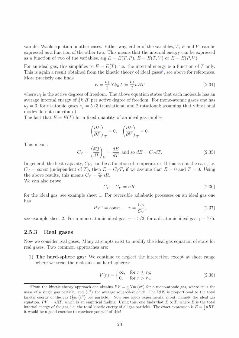
Now we consider real gases. Many attempts exist to modify the ideal gas equation of state forreal gases. Two common approaches are:

(i) The hard-sphere gas: We continue to neglect the interaction except at short rangewhere we treat the molecules as hard spheres:

V (r) =∞, for r ≤ r0;0, for r > r0.

(2.38)

1From the kinetic theory approach one obtains PV = 1

3Nm

⟨v2⟩for a mono-atomic gas, where m is the

mass of a single gas particle, and⟨v2⟩the average squared-velocity. The RHS is proportional to the total

kinetic energy of the gas (12m⟨v2⟩per particle). Now one needs experimental input, namely the ideal gas

equation, PV = nRT , which is an empirical finding. Using this, one finds that E ∝ T , where E is the totalinternal energy of the gas, i.e. the total kinetic energy of all gas particles. The exact expression is E = 3

2nRT ,

it would be a good exercise to convince yourself of this!

23

Figure 2.5: The van der Waals gas: schematic diagram of the interaction potential betweentwo molecules

Most of the ideal gas results continue to hold, but we have to make the replacementV → V − nb, where b is the ‘excluded volume’, proportional to the volume occupied byone mole of gas (i.e., b ∝ NAr

30). The equation of state for a hard sphere gas becomes

P (V − nb) = nRT, or P (V −Nβ) = NkBT, β =b

NA. (2.39)

(ii) The van der Waals gas: Apart from the hard-sphere interaction at short distance, wenow allow the weak intermolecular attraction at larger distances, as shown in Fig. 2.5.The extra attraction for r > r0 clearly reduces the pressure for a given V and T , since amolecule striking the vessel wall experiences an additional inward pull on this account.Call this intrinsic pressure π. So if the observed pressure is P and that expected if therewere no attraction is p, p− P = π, the hard-sphere equation of state

P =nRT

V − nb→ P + π =

nRT

V − nb.

Van der Waals argued that π is the result of mutual attraction between bulk of gas, i.e.,the tendency of molecules forming pairs, and hence should be proportional to N(N −1)/2 ∝ N2, or to N2/V 2 as it is intensive. Hence π = an2/V 2.

The equation of state for van der Waals gas is

(P + an2

V 2)(V − nb) = nRT

or

(P +αN2

V 2)(V −Nβ) = NkBT, (2.40)

where β = b/NA and α = a/N2A.

2.6 The zeroth law of thermodynamics and tempera-

ture*

2.6.1 The zeroth law

After the first law we now turn to the zeroth law. The terminology is due to the historicalorder in which things were developed. What is now known as the zeroth law was recognised

24

only after the first, second and third laws of thermodynamics had been named. The mostbasic concept in thermodynamics (or statistical mechanics) is temperature, and the zero-thlaw is required for a meaningful definition of temperature. In this sense the zero-th law is aprerequisite to the first, second and third law, hence calling in the ‘zero-th’ law is appropriate.What is temperature? We have an intuitive feel for it, but it is somewhat elusive. It isrelatively easy to understand what it means for a mass to be twice as large as another, or aforce which is twice as strong as another. But what does it mean to say that something istwice as hot as something else? All attempts to quantify this rest on

The zeroth law of thermodynamics:If a body C is in thermal equilibrium with A and with B, then A and B are also in thermalequilibrium with each other.

Why is this useful? We follow Young and Freedman, Chapter 17. Assume that C is athermometer, and that it is in thermal equilibrium with A and B. The thermometer thenmeasures the temperature of both A and B. But the reading would not change if A wereremoved, or if B were removed. Hence A and B have the same temperature. We can concludethat two systems are in thermal equilibrium with each other if and only if they have the sametemperature. This is what makes a thermometer useful. Technically speaking, a thermometermeasures its own temperature, but when in thermal equilibrium with another body, then itsown temperature is that of the other system.This is intuitively obvious, but it now permits the definition of something measurable, calledtemperature, whereby bodies in thermal equilibrium are at the same temperature.

2.6.2 Thermometers and temperature scales

To measure temperature we can use any property of matter that changes when heat is absorbedor emitted (e.g., resistance of a platinum wire, the volume (and hence length) of a volumeof liquid mercury in a glass tube, the pressure of a given quantity of gas in a fixed volume,etc.). Such devices can be used to verify the zeroth law experimentally. They are calledthermoscopes, for example the pressure of a given volume of an ideal gas is proportional totemperature. But since no scale has been defined, they are not yet thermometers.

A thermometer is a calibrated thermoscope. Any thermoscope can be used to define a numer-ical temperature scale over some range by using two fixed points (e.g., the ice freezing pointand boiling point of water). However, thermoscopes based on the volume of gases finally led tothe notion of an absolute scale based on a single fixed point. This is the ideal gas temperaturescale, measured in Kelvin (K) which is defined to be 273.16 K at the triple point of water (thesingle fixed point of the scale), agreed universally in 1954. Note: The freezing point of wateris some 0.01K lower (273.15 K) in temperature than the triple point (273.16 K).

Homework:A nice exposition of the details can be found in Young and Freedman, chapter 17.3, and youshould read it!

With such an absolute scale kBT (as in the ideal gas law) is a measure of thermal energy at theatomic scale; whereas RT is measure at the molar (macroscopic) scale. At room temperatureT ≈ 300K, kBT ≈ 1

40eV.

[Refs.: (1) Mandl Chap. 1.2, (2) Bowley and Sanchez Chap. 1.2, (3) Zemansky Chap. 1.]

25

Free telescopeThis page, when rolled into a tube, makes a telescope with 1 : 1 magnification.

26

Chapter 3

The second law of thermodynamics

“In this house, we obey the laws of thermodynamics!”(Homer Simpson)

“The law that entropy always increases, holds, I think, the supreme position amongthe laws of Nature. If someone points out to you that your pet theory of the uni-verse is in disagreement with Maxwell’s equations – then so much the worse forMaxwell’s equations. If it is found to be contradicted by observation – well, theseexperimentalists do bungle things sometimes. But if your theory is found to beagainst the second law of thermodynamics I can give you no hope; there is nothingfor it but to collapse in deepest humiliation.”(Sir Arthur Stanley Eddington, The Nature of the Physical World,1927)

3.1 Introduction

The basic observations leading to the second law are remarkably simple:

• When two systems are placed in thermal contact they tend to come to equilibrium witheach other - the reverse process, in which they revert to their initial states, never occursin practice.

• Energy prefers to flow from hotter bodies to cooler bodies (and temperature is just ameasure of the hotness). It is everyday experience that heat tends to flow from hot bodiesto cold ones when left to their own devices. There is a natural direction to spontaneousprocesses (e.g., the cooling of a cup of coffee)

• Physical systems, left to their own devices, tend to evolve towards disordered states,e.g. the mixing of milk in coffee. The reverse (spontaneous ordering) is not observed inclosed systems.

Note: These observations can be used to define a ‘direction of time’.

Related to this, it is important to realise that work and heat are simply different forms ofenergy transfer:

• Work is energy transfer via the macroscopically observable degrees of freedom. In thiscase the energy is transferred coherently.

27

• Heat is energy transfer between microscopic degrees of freedom. In this case the energyis transferred incoherently, the energy is stored in the thermal motion of the moleculesof the substance.

The second law says that there is an intrinsic asymmetry in nature between heat and work:extracting ordered motion (i.e. work) from disordered motion (i.e. heat) is hard1, whereas theconverse is easy. In fact the second law says that it is impossible to convert heat completelyinto work.

We will make these observations more quantitative through the introduction of a new statevariable, the so-called entropy, S. In classical thermodynamics, entropy ‘completes the set’of relevant thermodynamic variables (e.g., for a gas the complete set is (P, V, T, S) - anythingelse can be expressed in terms of these). However, the underlying deeper meaning of entropy(which is intrinsically a mysterious, deep and subtle concept) will only become clear when weprogress to statistical mechanics.

3.2 Heat engines and refrigerators

In order to introduce the concept of entropy it is useful to first consider heat engines andrefrigerators.

3.2.1 Heat engines

Heat engines run in cycles. In any one cycle the internal energy of the engines does not change,∆E = 0, by definition. During a cycle an amount of heat QH > 0 is absorbed from a hotsource (or set of hot sources; e.g., the hot combustion products in a car engine) and the enginedoes work w > 0 on its surroundings. During this process an amount of heat QC > 0 has beenemitted to a cooler thermal reservoir (or set of cooler reservoirs; e.g., the outside air). This isillustrated in Fig. 3.1.

Experimental observation: We can not make QC = 0, however hard we try (and engineershave tried very hard!). Even in the absence of frictional or dissipative processes (i.e., even fora reversible engine) we always have QC > 0.

From the first law we havew = QH −QC , (3.1)

given that ∆E = 0 in one cycle.

1In his 1848 paper titled ‘On an Absolute Thermometric Scale’ Kelvin writes: ‘In the present state ofscience no operation is known by which heat can be absorbed, without either elevating the temperature ofmatter, or becoming latent and producing some alteration in the physical condition of the body into whichit is absorbed; and the conversion of heat (or caloric) into mechanical effect is probably impossible, certainlyundiscovered.’ In a footnote he then goes on to say: ‘ This opinion seems to be nearly universally held by thosewho have written on the subject. A contrary opinion however has been advocated by Mr Joule of Manchester;some very remarkable discoveries which he has made with reference to the generation of heat by the frictionof fluids in motion, and some known experiments with magneto-electric machines, seeming to indicate anactual conversion of mechanical effect into caloric. No experiment however is adduced in which the converseoperation is exhibited; but it must be confessed that as yet much is involved in mystery with reference to thesefundamental questions of natural philosophy.’ Beautiful – TG.

28

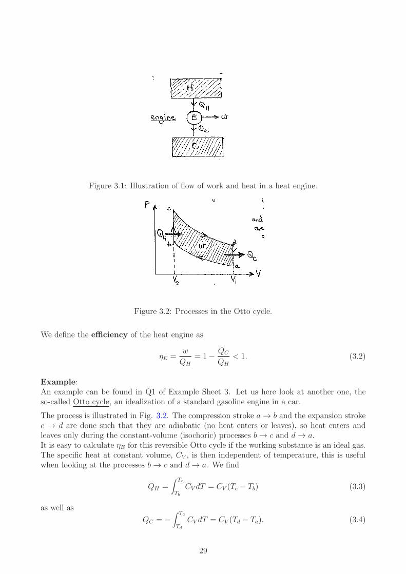
Figure 3.1: Illustration of flow of work and heat in a heat engine.

Figure 3.2: Processes in the Otto cycle.

We define the efficiency of the heat engine as

ηE =w

QH= 1− QC

QH< 1. (3.2)

Example:An example can be found in Q1 of Example Sheet 3. Let us here look at another one, theso-called Otto cycle, an idealization of a standard gasoline engine in a car.

The process is illustrated in Fig. 3.2. The compression stroke a→ b and the expansion strokec → d are done such that they are adiabatic (no heat enters or leaves), so heat enters andleaves only during the constant-volume (isochoric) processes b→ c and d→ a.It is easy to calculate ηE for this reversible Otto cycle if the working substance is an ideal gas.The specific heat at constant volume, CV , is then independent of temperature, this is usefulwhen looking at the processes b→ c and d→ a. We find

QH =∫ Tc

Tb

CV dT = CV (Tc − Tb) (3.3)

as well as

QC = −∫ Ta

Td

CV dT = CV (Td − Ta). (3.4)

29

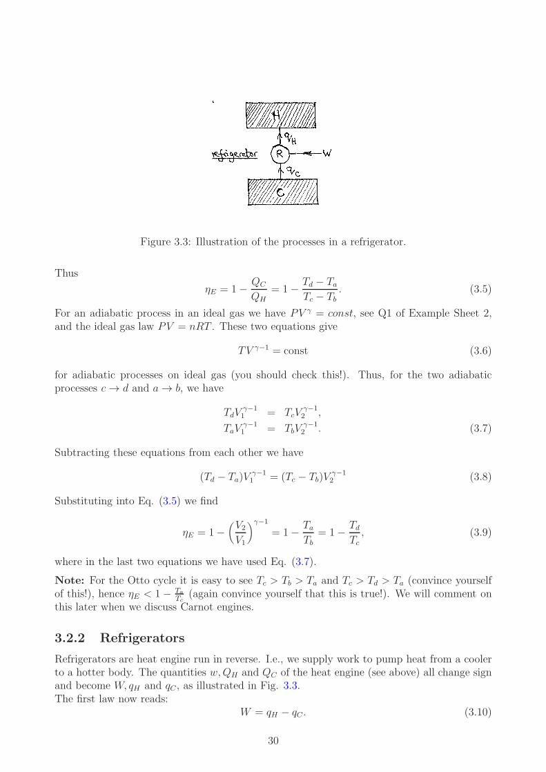
Figure 3.3: Illustration of the processes in a refrigerator.

Thus

ηE = 1− QC

QH= 1− Td − Ta

Tc − Tb. (3.5)

For an adiabatic process in an ideal gas we have PV γ = const, see Q1 of Example Sheet 2,and the ideal gas law PV = nRT . These two equations give

TV γ−1 = const (3.6)

for adiabatic processes on ideal gas (you should check this!). Thus, for the two adiabaticprocesses c→ d and a→ b, we have

TdVγ−11 = TcV

γ−12 ,

TaVγ−11 = TbV

γ−12 . (3.7)

Subtracting these equations from each other we have

(Td − Ta)Vγ−11 = (Tc − Tb)V

γ−12 (3.8)

Substituting into Eq. (3.5) we find

ηE = 1−(V2V1

)γ−1

= 1− TaTb

= 1− TdTc, (3.9)

where in the last two equations we have used Eq. (3.7).

Note: For the Otto cycle it is easy to see Tc > Tb > Ta and Tc > Td > Ta (convince yourselfof this!), hence ηE < 1 − Ta

Tc(again convince yourself that this is true!). We will comment on

this later when we discuss Carnot engines.

3.2.2 Refrigerators

Refrigerators are heat engine run in reverse. I.e., we supply work to pump heat from a coolerto a hotter body. The quantities w,QH and QC of the heat engine (see above) all change signand become W, qH and qC , as illustrated in Fig. 3.3.The first law now reads:

W = qH − qC . (3.10)

30

Examples of such machines are standard refrigerators, air-conditioners, and heat pumps.These are all essentially the same, but they have different purposes. Refrigerators and air-conditioners are used for cooling (e.g., the refrigerators cabinet, or a room), whereas the heatpump is used to heat (e.g., a room or a building). We now tailor the definition of efficiencyto the purpose. In general:

η =desired output

necessary input. (3.11)

(Note: Whereas the fact that QC 6= 0 is an unavoidable nuisance for a heat engine, the factthat qC 6= 0 means that refrigerators and heat pumps actually work!)

• For engines: desired output = w; necessary input = QH , hence

ηE =w

QH=QH −QC

QH. (3.12)

• For refrigerators: desired output = qC ; necessary input =W , hence

ηR =qCW

=qC

qH − qC. (3.13)

• For heat pumps: desired output = qH ; necessary input =W , hence

ηP =qHW

=qH

qH − qC. (3.14)

We note: ηE < 1 always (you should understand why), ηR > 1 usually, and ηP > 1 always(you should understand why). The quantities ηR and ηP (which can be greater than one)are sometimes called ‘coefficients of thermal performance’ because students are worried by‘efficiencies’ greater than one. Having a heat pump, as we have defined it would be pointless,if it had ηP < 1. If we have such heat pump we would not used it, instead we would just usean electric heater instead (efficiency of exactly one)!

Important remark:Real engines are optimized to perform forward or backwards, they are not reversible in thetechnical sense (there is friction, processes are not quasistatic). Thus relative sizes of W,QH

and QC will depend on the direction. However for idealized, reversible engines only the signswill change, and we have

ηP =1

ηE(for reversible engines/pumps). (3.15)

[Refs.: (1) Mandl 5.2, (2) Bowley and Sanches 2.3, (3) Zemansky 6.1-6.5.]

3.3 The second law of thermodynamics

There are two classic statements of the second law of thermodynamics.

Kelvin-Planck statement:It is impossible to construct an engine which, operating in a cycle, produces no effect other

31

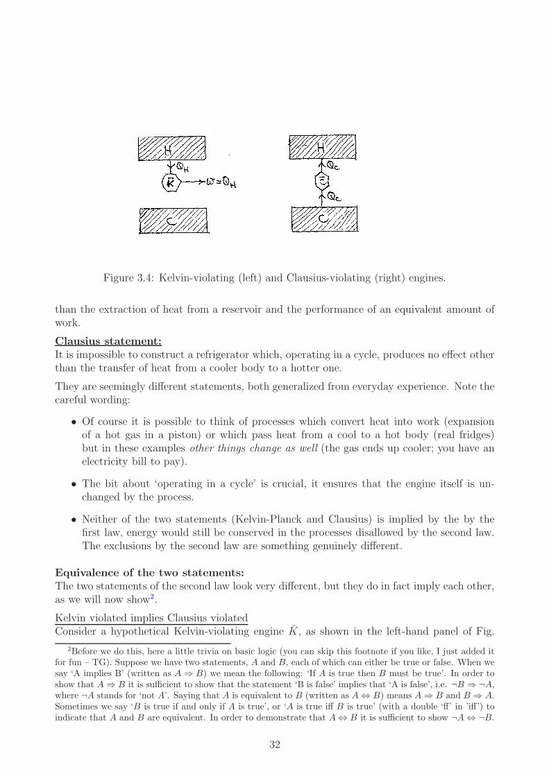
Figure 3.4: Kelvin-violating (left) and Clausius-violating (right) engines.

than the extraction of heat from a reservoir and the performance of an equivalent amount ofwork.

Clausius statement:It is impossible to construct a refrigerator which, operating in a cycle, produces no effect otherthan the transfer of heat from a cooler body to a hotter one.

They are seemingly different statements, both generalized from everyday experience. Note thecareful wording:

• Of course it is possible to think of processes which convert heat into work (expansionof a hot gas in a piston) or which pass heat from a cool to a hot body (real fridges)but in these examples other things change as well (the gas ends up cooler; you have anelectricity bill to pay).

• The bit about ‘operating in a cycle’ is crucial, it ensures that the engine itself is un-changed by the process.

• Neither of the two statements (Kelvin-Planck and Clausius) is implied by the by thefirst law, energy would still be conserved in the processes disallowed by the second law.The exclusions by the second law are something genuinely different.

Equivalence of the two statements:The two statements of the second law look very different, but they do in fact imply each other,as we will now show2.

Kelvin violated implies Clausius violatedConsider a hypothetical Kelvin-violating engine K, as shown in the left-hand panel of Fig.

2Before we do this, here a little trivia on basic logic (you can skip this footnote if you like, I just added itfor fun – TG). Suppose we have two statements, A and B, each of which can either be true or false. When wesay ‘A implies B’ (written as A ⇒ B) we mean the following: ‘If A is true then B must be true’. In order toshow that A ⇒ B it is sufficient to show that the statement ‘B is false’ implies that ‘A is false’, i.e. ¬B ⇒ ¬A,where ¬A stands for ‘not A’. Saying that A is equivalent to B (written as A ⇔ B) means A ⇒ B and B ⇒ A.Sometimes we say ‘B is true if and only if A is true’, or ‘A is true iff B is true’ (with a double ‘ff’ in ’iff’) toindicate that A and B are equivalent. In order to demonstrate that A ⇔ B it is sufficient to show ¬A ⇔ ¬B.

32

Figure 3.5: Construction to show that violating the Kelvin statement implies violating theClausius statement.

Figure 3.6: Construction to show that violating the Clausius statement implies violating theKelvin statement.

3.4. Now hook this engine up with regular (i.e., legal) refrigerator R, as shown in Fig. 3.5.This generates an ‘illegal’ refrigerator in the sense of the Clausius statement (see right-handpanel of Fig. 3.5).

Clausius violated implies Kelvin violatedNow consider a hypothetical Clausius-violating refrigerator C, as shown in the right-handpanel of Fig. 3.4. Combine this with a ‘legal’ engine, E, as shown in Fig. 3.6. This createsan ‘illegal’ engine in the sense of the Kelvin statement.

Thus we have shown the equivalence of the two statements of the second law.

[Refs.: (1) Mandl 2.1; (2) Bowley and Sanchez 2.2; (3) Zemansky 6.6-6.8]

3.4 Carnot cycles and Carnot engines

3.4.1 Background

In order to be realised in the real world, any reversible processes which involves a changeof temperature from an initial value to a final value would require an infinite number ofheat reservoirs at temperatures infinitesimally close to each other in order to keep everythingquasi-static. This does not sound very plausible.

33

However, there is a special form of heat engine which only relies on two reservoirs: a hot one attemperature TH , and a cold one at TC < TH . Reversible engines with only two such reservoirswill play a very important role in later on in this course. We may wonder, e.g.,

(i) What is the maximum ηE that can be achieved for a given TH and TC?

(ii) What are the characteristics of such maximally efficient engines?

(iii) Of what effect is the nature of the working substance in such maximally efficient engines?

These questions were all answered by Sadi Carnot, and heat engines of this type are knownas ‘Carnot engines’, or the ‘Carnot cycle’.

3.4.2 Carnot engines and Carnot’s theorem

Definition:A Carnot engine is a reversible engine acting between only two heat reservoirs. That meansthat all processes are either isothermal (heat transfer at a constant temperature) or adiabatic(no heat transfer).

Carnot’s theorem:A reversible engine operating between two given given reservoirs is the most efficient enginethat can operate between those reservoirs.

We will prove this below. Before we do this, let us re-phrase the theorem. Carnot’s theoremsays that a reversible engine is the most efficient engine which can operate between tworeservoirs.

Much is made of the fact that the Carnot engine is the most efficient engine. Actually,this is not mysterious. First, if we specify only two reservoirs, then all it says is that areversible engine is more efficient than an irreversible engine, which isn’t all that surprising(no friction...) Second, we will see that the efficiency of a Carnot engine increases with thetemperature difference between the reservoirs. So it makes sense to use only the hottest andcoldest heat baths you have available, rather than a whole series of them at intermediatetemperatures. But the independence of the details of the engine is rather deeper, and hasfar-reaching consequences.

Proof of Carnot’s theorem:The construction used to prove the theorem is illustrated in Fig. 3.7. The green engines/pumpsare Carnot (reversible), and the brown ones are irreversible.Assume there is an engine E which is more efficient than a Carnot engine, i.e. ηE > ηC . TheCarnot engine is reversible, and so it can be run as a pump, see left-hand panel of Fig. 3.7.Since ηE > ηC , we have

W

Q′H

>W

QH, (3.16)

i.e. QH > Q′H . From the first law

W = Q′H −Q′

C = QH −QC . (3.17)

34

Figure 3.7: Left: Construction to prove Carnot’s theorem. Right: Construction used toprove that all reversible engines operating between two reservoirs have the same efficiency, ηC .

We concludeQH −Q′

H = QC −Q′C . (3.18)

Because of QH > Q′H these quantities are both positive. But this means that a net amount

of heat, QH −Q′H = QC −Q′

C > 0 is pumped from the colder reservoir to the hotter reservoirby the combined system. This violates the Clausius statement.

Corollary of Carnot’s theorem:Any reversible engine working between two heat reservoirs has the same efficiency as anyother, irrespective of the details of the engine.

Proof:Consider a Carnot engine, C, maximising the efficiency for two given reservoirs, and anotherreversible engine, E, operating between the same two reservoirs. Its efficiency is ηE ≤ ηC , asC is the most efficient engine for these two reservoirs. We want to show that ηE = ηC , soassume that ηE is strictly smaller than ηC , and construct a contradiction.So assume ηE < ηC . Run the engine in reverse, and connect it to a Carnot engine, as shownin the right-hand panel of Fig. 3.7. We have

ηE =W

Q′′H

<W

QH= ηC . (3.19)

This implies Q′′H > QH . From the first law we have W = QH − QC = Q′′

H − Q′′C , and so it

followsQH −Q′′

H = QC −Q′′C , (3.20)

and both of these quantities are negative. Thus, Q′′H − QH = Q′′

C − QC > 0. This meansthat the combined system pumps heat from the cold reservoir to the hot reservoir, which isin violation of Clausius’ statement. So we have the desired contradiction. This completes theproof of the corollary.

This is a remarkable (and deep) result. It means that, for two reservoirs with temperaturesTH and TC , any reversible engine has the same efficiency, and that this efficiency is a function

35

Figure 3.8: The Carnot cycle for an ideal gas.

of the temperatures of the two reservoirs only, ηC = ηC(TH , TC). In particular the efficiencyis independent of working substance, e.g., the working substance could be an ideal gas, a realgas, a paramagnet, etc. We can evaluate the efficiency for any substance and we would alwaysobtain the same result. So we choose the simplest possible substance, an ideal gas.

3.4.3 Calculating the efficiency of a Carnot cycle

Consider a cycle as shown in Fig. 3.8:

• a → b: isothermal compression in contact with a reservoir at temperature TC ; heat QC

emitted;

• b→ c: adiabatic compression (no reservoirs; no heat flow);

• c → d: isothermal expansion in contact with reservoir at temperature TH , heat QH

absorbed;

• d→ a: adiabatic expansion.

The first law statesdQ = dE − dW = dE + PdV (3.21)

for reversible process. For the ideal gas, we have E = E(T ) and so dE = 0 along an isotherm.Hence dQ = nRT dV

Valong isotherms. Therefore we have

QC = −∫ b

anRTC

dV

V= nRTC ln

VaVb

(3.22)

along a→ b (convince yourself that this is of the right sign!), and

QH =∫ d

cnRTH

dV

V= nRTH ln

VdVc

(3.23)

along c→ d.

The efficiency is then

ηCE ≡ 1− QC

QH

= 1− TCTH

ln(Va/Vb)

ln(Vd/Vc). (3.24)

Next we use that TV γ−1 = const for adiabatic processes on an ideal gas (with γ = CP/CV asusual). For the two adiabatic processes b→ c and d → a we therefore have

TCVγ−1b = THV

γ−1c

TCVγ−1a = THV

γ−1d . (3.25)

36

From this we conclude (Va/Vb)γ−1 = (Vd/Vc)

γ−1, i.e.

VaVb

=VdVc. (3.26)

Substituting this into Eq. (3.24) we find

ηCE = 1− TCTH

. (3.27)

This is the efficiency of a Carnot engine with an ideal gas as a working substance.Using the above corollary we conclude that Eq. (3.27) holds for all Carnot engines operatingbetween these two reservoirs.

Using the definition of efficiency, Eq. (3.24) we can further derive an important general rela-tion, the so-called

Carnot relationQC

TC=QH

TH, (3.28)

applicable to Carnot engines.

In the following, we will discuss several examples involving heat engines.

Example 1:A power station contains a heat engine operating between two reservoirs, one comprising steamat 100C and the other comprising water at 20C. What is the maximum amount of electricalenergy which can be produced for every Joule of heat extracted from the steam?

Solution:The maximum w comes from a Carnot engine. We have QH −QC = w and QH/TH = QC/TC .Hence

w = QH

(1− TC

TH

).

Insert QH = 1J , TC = 293K, TH = 373K and obtain

w = 1J ×(1− 293K

373K

)= 0.21J. (3.29)

Example 2:A refrigerator operating in a room at 20C has to extract heat at a rate of 500 W from thecabinet at 4 C to compensate for the imperfect insulation. How much power must be suppliedto the motor if its efficiency is 80% of the maximum possible?

Solution:To make our lives a little bit easier we will operate with energy and heat transferred persecond, and indicate this by a ‘dot’, i.e. W , qH , etc. The minimum Wmin comes from aCarnot refrigerator. We have

Wmin = qH − qC , (3.30)

as well asqHTH

=qCTC

. (3.31)

37

hence

Wmin = qC

(THTC

− 1).

Insert qC = 500 W, TC = 277 K,TH = 293 K and find

Wmin = 500W× 16

277= 28.9W. (3.32)

But the real refrigerator works at 80% of maximum efficiency, so we have Wreal = Wmin/0.8 =36.1 W.

A few things to think about: Do you know how a real refrigerator works? What is the commonworking substance used? Can efficiency of a refrigerator (as defined above) be greater thanone?

[Refs.: (1) Mandl 5.2; (2) Bowley and Sanchez 2.3; (3) Zemansky 7.1-7.4]

3.5 The thermodynamic temperature scale*

We have already seen how to define temperature based on the properties of an ideal gas, seeSec. 2.6.2. Essentially you do the following: take water to the triple point, and put it inthermal equilibrium with a container of volume V , and with n moles of an ideal gas in it. Callthe pressure you measure Ptriple. Now to define the temperature of something else, put thatsomething else in contact with the same container of n moles of an ideal gas, and with volumeV . You will measure a different pressure. The ideal-gas temperature of the ‘something’ is thendefined as T = TtripleP/Ptriple. The parameter Ttriple sets the scale, and it is, by convention,set to Ttriple = 273.16 K.

Now this whole process relies on the properties of the ideal gas. We now want to define atemperature scale which does not depend on the properties of a specific working substance.

To this end we use the properties of the Carnot cycle. We know that any Carnot engine operat-ing between two fixed reservoirs will have the sam efficiency regardless of the working substanceof the engine:

ηCarnot = 1− QC

QH, (3.33)

where QH and QC are the amounts of heat extracted per cycle from the hot reservoir andrejected into the cold reservoir, respectively. It was Kelvin’s idea to use this principle to definea temperature scale: Supposed you have a system A of which you would like to determinethe temperature. Use this system as one of the reservoirs of a Carnot engine. For the otherreservoir use a system, B, in thermal equilibrium with water at the triple point. Then measurethe amounts of heat flowing out of/into systems A and B in one cycle of the Carnot engine.Then define

ΘA =|QA||QB|

Θtriple. (3.34)

In other words this definition of ΘA can be written as

ΘA = Θtriple (1− η(A,B)) , (3.35)

where η(A,B) is the efficiency of Carnot engine running between A and B.

38

Again, Θtriple is a parameter setting the overall scale, but other than that we have not used anyproperties of any working substance, only the properties of a generic Carnot engine. Givena heat bath at a reference temperature (e.g. a very large triple-point cell) we can use theefficiency of a Carnot engine working between it and another body to label that other body’stemperature.If we use the ideal gas temperature scale, then we know

ηCarnot = 1− TCTH

(3.36)

for a Carnot engine operating between reservoirs with absolute temperatures TC and TH . Thiswas Kelvin’s idea in 1848, and it is referred to as a ‘thermodynamic temperature scale’. Theword ‘thermodynamic’ here indicates that one does not use the properties of a particularworking substance, but only those of general Carnot engines. And these in turn are derivedfrom the laws of thermodynamics.We can make this argument more formal. Say we have an arbitrary temperature scale, ϑ, suchthat

θ1 > θ2 ⇔ body 1 is hotter than body 2. (3.37)

Now look at three thermal baths of temperatures θC < θI < θH in this arbitrary scale.Construct two Carnot engines, one operating between θH and θI , the other between θI andθC , as shown on the left in Fig. 3.9. We construct these engines such that the heat transferredinto the intermediate heat bath is of the same magnitude as the heat taken out of that heatbath by the other (this is labelled QI in the figure). Now, the efficiencies of these two enginesare

ηHI = 1− QI

QH,

ηIC = 1− QC

QI

. (3.38)

Given the universality of the efficiencies of Carnot engines, any reversible engine between thesereservoirs would have the same efficiencies, regardless of their working substances. So theseefficiencies can only depend on temperature:

ηHI = 1− f(θI , θH)

ηIC = 1− f(θC , θI), (3.39)

with some unknown function f(·, ·).Next, we look at the construction on the left-hand-side of the figure as a whole. Effectively, thecomposite system (made of the two engines we have discussed) is a reversible engine operatingbetween QC and QH . That engine must then have efficiency

ηHC = 1− f(θC , θH). (3.40)

Now, assume we use some different temperature scale, θ. Then we have θC = θ(TC) andθH = θ(RH). The mapping between θ and T is assume to be one-to-one. The efficiency of theCarnot engine can then be expressed in terms of θC and θH , let’s say

ηCarnot = 1− f(θC , θH), (3.41)

39

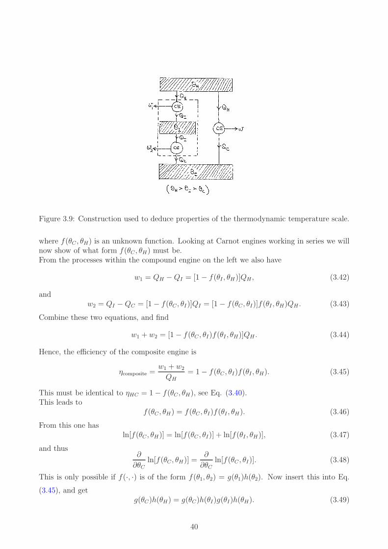
Figure 3.9: Construction used to deduce properties of the thermodynamic temperature scale.

where f(θC , θH) is an unknown function. Looking at Carnot engines working in series we willnow show of what form f(θC , θH) must be.From the processes within the compound engine on the left we also have

w1 = QH −QI = [1 − f(θI , θH)]QH , (3.42)

andw2 = QI −QC = [1− f(θC , θI)]QI = [1− f(θC , θI)]f(θI , θH)QH . (3.43)

Combine these two equations, and find

w1 + w2 = [1− f(θC , θI)f(θI , θH)]QH . (3.44)

Hence, the efficiency of the composite engine is

ηcomposite =w1 + w2

QH= 1− f(θC , θI)f(θI , θH). (3.45)

This must be identical to ηHC = 1− f(θC , θH), see Eq. (3.40).This leads to

f(θC , θH) = f(θC , θI)f(θI , θH). (3.46)

From this one hasln[f(θC , θH)] = ln[f(θC , θI)] + ln[f(θI , θH)], (3.47)

and thus∂

∂θCln[f(θC , θH)] =

∂

∂θCln[f(θC , θI)]. (3.48)

This is only possible if f(·, ·) is of the form f(θ1, θ2) = g(θ1)h(θ2). Now insert this into Eq.

(3.45), and getg(θC)h(θH) = g(θC)h(θI)g(θI)h(θH). (3.49)

40

From this we get

g(θ) =1

h(θ), (3.50)

and thus f(·, ·) must be of the form

f(θ1, θ2) =g(θ1)

g(θ2). (3.51)

We find

ηCarnot = 1− g(θ1)

g(θ2)(3.52)

for any Carnot engine operating between θ1 and θ2. The function g is at this point stillarbitrary, it is determined by our choice of temperature scale, θ. Or vice versa, any choice ofg defines a temperature scale, θ.

The absolute Kelvin scale corresponds to a linear function g(θ) = θ,

Kelvin scale : ηCarnot = 1− θ1θ2. (3.53)

Comparison with Eq. (3.36) shows that the absolute Kelvin scale θ (defined by g(θ) = θ) mustbe proportional to the ideal-gas absolute temperature, i.e. θ = αT , where T is the absoluteideal-gas temperature and α a constant. Clearly α = 1 if we define θtriple = Ttriple = 273.16 K.This is in fact the convention Kelvin chose.

[Refs.: (1) Bowley and Sanchez 2.3-2.4; (2) Zemansky 7.5]

3.6 Entropy and maximum-entropy principle

3.6.1 Clausius’ Theorem

The extremely important result which we now prove is the following theorem.

Clausius’ TheoremIf a system is taken through a cycle, the algebraic sum of the heat added weighted by theinverse of the temperature at which it is added, can never be greater than zero,

∮dQ

T≤ 0 . (3.54)

The equality holds if the process is reversible, i.e.

∮dQrev

T= 0 . (3.55)

Proof:We follow Blundell and Blundell, Concepts in Thermal Physics, Oxford University Press.Thetheorem can be derived from the second law as follows:Consider a Carnot engine, C, operating between a heat reservoir at temperature T0 and asecond system at temperature Ti. We consider a cyclic process. In each cycle the temperature

41

Figure 3.10: Construction used to prove Clausius’ Theorem.

of the second system goes through a sequence of temperatures, T1, T2, . . . , TN , this is wherethe label Ti comes from in Fig. 3.10. In the time element of the cycle during which the systemis at Ti and amount of heat dQi is transferred from the Carnot engine to the system at Ti, atthe same time C does an amount of work dWC

i . Using the first law the amount of heat theCarnot engine extracts from the reservoir at T0 must then be dWC

i + dQi. At the same timewe assume that the system Ti does an amount of work dWi on the environment during thispart of the cycle.Our strategy is to prove that

∑Ni=1

Qi

Ti≤ 0, and we will then take the limit N → ∞ to obtain

Clausius’ Theorem.

For the Carnot engine we know that during the time interval i:

heat to reservoir at TiTi

=heat from reservoir at T0

T0, (3.56)

i.e.dQi

Ti=dQi + dW

Ci

T0. (3.57)

From this we find

dWCi = dQi

(T0Ti

− 1). (3.58)

Of course the whole setup in Fig. 3.10 looks very suspicious, from the figure it seems thatwhat the system does in any one cycle is to extract heat from T and to convert it fully intowork. This is forbidden by the second law (Kelvin’s statement). So some of the quantities inthe figure must be negative. More precisely

total work produced per cycle =n∑

i=1

(dWCi + dWi), (3.59)

42

and this quantity cannot be positive. So

N∑

i=1

d(WCi + dQi) ≤ 0, (3.60)

where we have used∑

i dWi =∑

i dQi. Using relation (3.57) we find

T0N∑

i=1

dQi

Ti≤ 0, (3.61)

and so (since T0 > 0):N∑

i=1

dQi

Ti≤ 0. (3.62)

Taking the limit N → ∞, we replace the sum by an integral and obtain

∮dQ

T≤ 0, (3.63)

keeping in mind that we are operating a cyclic process.

If the process is reversible, we have ∮dQ

T= 0. (3.64)

To demonstrate this, reverse all arrows in Fig. 3.10, i.e. all quantities change sign. The totalwork done per cycle is then

total work produced per cycle = −n∑

i=1

(dWCi + dWi). (3.65)

Using the second law we require

−n∑

i=1

(dWCi + dWi) ≤ 0, (3.66)

which leads to

−N∑

i=1

dQi

Ti≤ 0. (3.67)

This, together with∑N

i=1dQi

Ti≤ 0 means that

N∑

i=1

dQi

Ti= 0. (3.68)

This completes the proof.

Remark:Clausius’ theorem is easily verified for Carnot cycles, since for these heat only enters or leavesat one of two temperatures. One has

∮

Carnot

dQ

T=QH

TH− QC

TC= 0, (3.69)

where we have used Eq. (3.28) for the second equal sign.

43

3.6.2 Entropy and the maximum-entropy principle

Definition and function-of-state property

We are now in a position to introduce the concept of entropy. For a given system, the changein entropy for an infinitesimal reversible change is defined by

dS =dQ

T. (3.70)

It follows from Clausius’ theorem (which in turn was derived from the second law) that S isa function of state.

Proof:We have seen that ∮

dQ

T= 0 (3.71)

for all reversible processes. Now consider an initial state, i, and a final state f of a system,and two reversible paths from i to f . Call these paths A and B. What we need to show isthat the integral

∫ fi dS does not depend on the path. We use a standard argument: go from

i to f using path A, and then back from f to i using the reversed path of B. This defines acycle, so the total change of entropy is zero along the cycle. Get

0 =∮dS =

∫

path AdS −

∫

path BdS (3.72)

and soS(state f)− S(state i) =

∫

path AdS =

∫

path BdS. (3.73)

=⇒ The entropy S is a function of state.

Maximum-entropy principle

We have introduced dS = dQ/T for reversible processes, and seen that∮dS = 0 if all processes

along the cycle are reversible. What about other processes? By considering a cycle consistingof one reversible and one irreversible process (see Fig. 3.11), we can show that in general,

dQ ≤ TdS. (3.74)

To see this, consider Fig. 3.11. From the reversible path we have

S2 − S1 =∫ 2

1

dQrev

T. (3.75)

What can we say about an irreversible process between the same endpoints? Clearly theentropy change is the same (that’s what we mean by saying entropy is a function of state.)But if we consider a cycle involving an irreversible process from 1 to 2 and a reversible processto return to 1, we have a cycle for which Clausius’s theorem holds:

∮dQ

T< 0 (3.76)

44

Figure 3.11: Construction used to show dS ≥ dQT.

Decomposing∮ dQ

T=∫ 21

dQirrev

T+∫ 12

dQrev

Twe find

∫ 2

1

dQirrev

T<∫ 2

1

dQrev

T=∫ 2

1dS. (3.77)

From this we concludedQ ≤ TdS. (3.78)

Summary:If an amount of heat dQ is supplied to a system from a source at temperature T , then thechange in the entropy of the system satisfied the inequality

dS ≥ dQ

T. (3.79)

The equality applies if the process is reversible.

Isolated systems:If a system is thermally isolated dQ = 0. This means that

dS ≥ 0 for thermally isolated systems (3.80)

=⇒ The entropy of an isolated system cannot decrease.This is an alternative statement of the second law. Note: Any system plus its surroundings(in thermodynamics deliberately called by the somewhat grandiose title ‘the universe’) formsan isolated system. Hence we have another statement:

The entropy of the universe never decreases.

What this means is that any decrease in the entropy of a system must be at least compensatedby an increase in the entropy of its surroundings.We can now turn to the

Maximum-entropy principle

45

An isolated system at equilibrium must be in the state of maximum entropy.

‘Proof’:This can be seen as follows: For thermally isolated systems we have dS ≥ 0 as seen above. Inequilibrium state functions do not change, and so we have dS = 0. Hence it is clear that theentropy of an isolated system increases as an equilibrium is approached. It reaches a constantand maximum value when equilibrium is achieved.

Example:Gas particles expand from volume V0 to 2V0 in an adiabatically isolated container.

Remark:The more disordered the system, the greater the entropy. This will become more clear (clearer?) later when we define entropy from microscopic principles. The increase of entropy in everynatural irreversible process measures the increase of disorder, or randomness in the universe,associated with that process.

Another remark:In the next section, we will exploit the fact that entropy is a state function (process inde-pendent) when we calculate the entropy change for an irreversible process by considering areversible process with the same initial and final states. This is the key idea in most ques-tions on entropy calculations. Make sure you understand it, then exploit it when you do theproblems on the example sheets.

[Refs.: (1) Bowley and Sanchez 2.5,2.7; (2) Zemansky 8.1-8.2, 8.8-8.9]

3.6.3 Examples involving entropy changes

We will now look at a few prototypical examples of processes involving changes of entropy.These demonstrate (among other things) that, in general,

• the entropy of any system increases when it is heated, and

• the entropy of gas increased when it expands at constant temperature.

A common theme (which we will explore in much more detail later) is that an increase inentropy means an increase in disorder. We will see that the entropy of the universe alwaysincreases during spontaneous changes (typical example are the flow of heat from a hotter to acooler body and the free expansion of a gas). In these examples the total entropy increases,although that of parts of the system may decrease.Heat flow from hotter to colder bodies is irreversible, and reversible processes must involve heatflow between bodies at the same temperature or only infinitesimally different. The entropychange of the system

dSsystem =dQrev

T(3.81)

must be exactly balanced by that of the heat bath

dSreservoir = −dQrev

T(3.82)

so that dSuniverse = 0.

46

For adiabatic process no heat flows dQ = 0. Thus, dS = dQrev/T and dS = 0 for any reversible,adiabatic process. We say a process is isentropic if it is adiabatic and reversible.

In summary:

• ∆Suniverse > 0 for spontaneous changes

• ∆Suniverse = 0 for reversible changes, during which

∆Ssystem = −∆Ssurroundings

• Spontaneous changes are always irreversible

• Isentropic change ⇔ reversible, adiabatic changes, dS = 0.

Example 1:Two identical blocks of metal, one at 100 C and the other at 0 C are put in thermal contact.Derive the total entropy change when equilibrium is re-established. (You may assume that theheat capacity, C, of each block is constant over this temperature range, and you may neglectvolume changes.)

Solution:Clearly heat will flow from hotter to cooler body until they have the same temperature. Byconservation of energy this will be 50 C. The heat transfer occurs so as to maximise thatentropy. So, if dQ is transferred from the hot body at TH to the cold one at TC

dSC >dQ

TC, dSH > −dQ

TH, (3.83)

and

dStotal = dSH + dSC >(

1

TC− 1

TH

)dQ > 0. (3.84)

Thus, the entropy decrease of the hot block is more than compensated by the entropy increaseof the cold block =⇒ the spontaneous heat flow is associated with a net (overall) entropyincrease.In order to calculate ∆Stotal we use the following strategy: we cannot calculate ∆S for irre-versible process, so we must find a reversible process that takes us from the same initial tothe same final end point. Then, since ∆S is independent of the actual process (you should beable to say why is this so), this will suffice. For heating or cooling of the blocks this wouldinvolve a quasistatic process of bringing the blocks into contact with an infinite sequence ofheat baths at infinitesimally increasing or decreasing temperature, so that the temperaturedifference between the heat bath and the block is always negligible and the entropy change iszero.

∆S =∫ 2

1

dQrev

T, (3.85)

where dQrev = CdT . But if C =const,

∆S = C∫ 2

1

dT

T= C ln

T2T1. (3.86)

47

Thus, in our case of two identical blocks

∆Stotal = ∆SC +∆SH = C lnTfTC

+ C lnTfTH

= C lnT 2f

TCTH. (3.87)

Inserting the values TH = 373 K, TC = 273 K, Tf = 323 K,

∆Stotal = C ln(323K)2

373K × 273K= 0.024C. (3.88)

Note: ∆Stotal > 0, as required; and that the unit of entropy = unit of heat capacity = J K−1.

Example 2:Two identical blocks of metal, one at 100 C and the other at 0 C are brought into thermalcontact. What is the maximum amount of work w that can be extracted from the hot blockin the absence of other heat sinks, expressed as a fraction of the total heat loss QH of the hotblock?

Solution:Clearly, we can’t just extract heat from the hot block an turn it all into work, since this wouldviolate the second law. In this process ∆SH < 0. We need to add at least enough heat QC tothe cold block so that ∆SC > 0 just balances ∆SH , i.e. we can make ∆SC +∆SH = 0. Notethe work extracted can always be used to do things which lead to zero entropy change (e.g.,raising a weight). Once the two blocks come to the same final temperature Tf no further workcan be extracted. From Example 1,

∆Stotal = ∆SH +∆SC = C ln

(T 2f

THTC

)≥ 0. (3.89)

The maximum work possible corresponds to the lowest possible Tf (see equation for work wbelow). The lowest possible Tf is that for which ∆Stotal = 0, viz.

Tf =√THTC ≈ 319.1K = 46.1 C. (3.90)

(If Tf were any lower ∆Stotal < 0 and this isn’t allowed by the 2nd law). Now

QH = C(TH − Tf), QC = C(Tf − TC). (3.91)

Hence, by energy conservation, the work extracted is

w = QH −QC = C(TH + TC − 2Tf) = C(TH + TC − 2√THTC). (3.92)

The efficiency then comes out as

η =w

QH

=TH + TC − 2

√THTC

TH −√THTC

=(√TH −

√TC)

2

√TH(

√TH −

√TC)

= 1−√TCTH

. (3.93)

48

Inserting the values TH = 373 K, TC = 273 K

w =

(1−

√THTC

)QH = 0.144QH . (3.94)

i.e., only 14.4% of the heat lost by the initially hot block is available to do work. Note,too, that this maximum efficiency is obtained from a reversible process. [Compare with thecorresponding efficiency η = 1 − TC/TH = 26.8% for a Carnot engine working between two(infinite) reservoirs at fixed temperatures TH = 373 K, TC = 273 K.]

Example 3 [Heat engines revisited]:From the law of the non-decrease of entropy, show that the maximum efficiency of a heatengine operating between two (infinite) reservoirs at fixed temperatures TH and TC occurswhen the engine is reversible.

Solution:The change in entropy of the total engine

∆Stotal = ∆SC +∆SH =QC

TC− QH

TH≥ 0. (3.95)

HenceQC

QH

≥ TCTH

, (3.96)

with equality for ∆S = 0, i.e. for a reversible process. The efficiency is

η =w

QH= 1− QC

QH≤ 1− TC

TH, (3.97)

with a maximum for equality (i.e., for a reversible engine). This is of course Carnot’s theorem,which we have now re-derived from the law of a non-decreasing entropy.

Example 4:A quantity of n moles of an ideal gas at temperature T0 is initially confined to half the volumeof an thermally insulated container by an insulated partition. The partition is removed withoutdoing any work. What is the ensuing change of entropy?

Solution:The process is adiabatic, so dQ = 0. However, we recall, this does not imply dS = 0 since thisis not a reversible process. Once again we need to find a reversible process to go from sameinitial to same final point. As we saw earlier (and see, e.g. Q1(b) on Example Sheet 1), thiscould be an isothermal expansion done reversibly. In such an expansion

Qrev = −W rev =∫ 2

1PdV =

∫ V2

V1

nRT0V

dV = nRT0 lnV2V1

(3.98)

Put V2 = 2V1 as in this problem

∆S =Qrev

T0= nR ln 2. (3.99)

Note: The logic here is quite subtle - do make absolutely sure you understand the differencebetween the actual process (with Q = W = 0) and the reversible process for which we areable to calculate ∆S (that process has Qrev = −W rev 6= 0).

49

Example 5a: A box of gas is joined by an identical box of the same gas. What is the changein total entropy?Solution: This is a reversible process (as nothing changes when removing the partition andputting it back). Total entropy change is therefore zero, ∆Stotal = 0, where Stotal = S1 + S2 =2S1.

The following example is an irreversible process (How?) and the total entropy must increase.Example 5b:An insulated container is originally divided in half by a partition, and each half is occupiedby n moles of two different ideal gases at temperature T0. What is the total change in entropywhen the partition is removed without doing any work?

Solution:Since both gases are ideal, they don’t interact, each species is oblivious of the other, and ∆Sfor each is exactly as in Ex. 4 above. Thus

∆Stotal = 2nR ln 2. (3.100)

Note: the total mixing - which we know will happen eventually - is precisely the change thatnow maximises the entropy, i.e., a clear hint that entropy means disorder. It is obvious thatthe process is an irreversible one as the situation is quite different from the initial state whenputting back the partition after the two gases have mixed.

[Refs.: (1) Mandl 4.3, (2) Bowley and Sanchez 2.8; (3) Zemansky 8.11-8.13]

3.7 The arrow of time

An apparent paradox arises from the second law of thermodynamics:

• Phenomena in the macroscopic world are obviously irreversible.

• But microscopic laws (e.g. Newton’s equations, quantum mechanics, Maxwell’s equa-tions, . . . ) are unchanged by replacing t by −t.

Can this paradox be resolved using statistical thermodynamics?

We know that dS ≥ 0 for isolated systems, and dS > 0 for irreversible processes of suchsystems. This defines an arrow of time. Eddington stated this as follows (1928):

“Let us draw an arrow arbitrarily. If as we follow the arrow we find more andmore of the random element in the state of the world, then the arrow is pointingtowards the future; if the random element decreases the arrow points towards thepast. [. . . ] I shall use the phrase times arrow to express this one-way property oftime which has no analogue in space.”

Consider a typical irreversible situation (see Fig. 3.12), the time dependence of the entropy isshown in Fig. 3.13.Now imagine removing the partition at t = 0, and follow particle trajectories into the past.The fundamental laws of microscopic physics are unchanged under t → −t, so the same

50

Figure 3.12: An irreversible process, removal of a barrier separating two sets of identicalparticles.

Figure 3.13: Time-dependence of the entropy in the process illustrated in the previous figure.

Figure 3.14: Hypothetical entropy in the past.

51

uniform distribution would be found at t = −tf as at t = +tf . This leads to a hypotheticalentropy in the past as shown in Fig. 3.14. This looks completely symmetric with respect totime-reversal.

However, starting in the disordered (high-entropy) state at t = −tf we would never observethe ordered state at later times. If the initial state is one of maximum entropy, then theentropy would remain constant with time.

‘Resolution’ of the paradox:So the problem only ever arises if the initial state has an entropy less than the maximumentropy. So one can argue the fact that we see an ‘arrow of time’ means that the initial stateof our universe must have been one of low entropy, i.e. it was very ordered. In our dailyphysics experience we find that such states need special preparation, e.g. the low-entropystate in the above de-mixing example requires all particles to be on one side of the partition.

Problem:There is no current theory which would explain a low-entropy early universe. And at thispoint the paradox is now the cosmologists’ problem.

52

Chapter 4

The mathematical structure of thetheory of thermodynamics

“The miracle of the appropriateness of the language of mathematics for the formu-lation of the laws of physics is a wonderful gift which we neither understand nordeserve.”(Eugene Wigner, 1960)

“Mathematics Is Biology’s Next Microscope, Only Better. [. . . ] Those who un-derstand the calculus, ordinary and partial differential equations, and probabilitytheory have a way of seeing and understanding the world, including the biologicalworld, that is unavailable to those who do not.1”(Joel E. Cohen, 2004)

4.1 Mathematical tools

4.1.1 Differentials

Differentials

Consider a function f = f(x) of one variable. Taylor expanding about a point x then gives

f(x+∆x)− f(x) = f ′(x)∆x+ . . . (4.1)

where . . . stands for higher order terms in ∆x. For infinitesimal ∆x we write dx, and weintroduce df = f(x+ dx)− f(x). We then have

df = f ′(x)dx. (4.2)

1You may wonder why I use this quote in a set of lecture notes for thermal and statistical physics. This isnot a course on mathematics, let alone biology, after all. But when Cohen says ‘ordinary and partial differentialequations’, well that’s what you learn in physics courses on classical mechanics or electrodynamics, or indeedin third-year nonlinear physics. And when he says ‘probability theory’, well that’s what you discuss in RandomProcesses, in this course here or in the fourth-year module on advanced statistical physics. The contributionsto biology made by those trained in these subjects are tremendous, and much of the progress of modern biologywould be impossible without them. Also, I like the title of the paper very much, ‘Mathematics Is Biology’sNext Microscope, Only Better’. Just brilliant. TG.

53

If f is a function of multiple variables, x1, x2, . . ., we have the analog expression

df =∂f

∂x1dx1 +

∂f

∂x2dx2 + . . . (4.3)

This is what is called the total differential of f .Next, consider the more general expression

du = a1(x1, x2, . . .)dx1 + a2(x1, x2, . . .)dx2 + . . . . (4.4)

Expressions of this type are also called differentials, but notice the difference compared to Eq.(4.3). The expression in (4.4) is more general, as the functions a1, a2, . . . can be arbitrary. InEq. (4.3) they have to be the partial derivatives of a common function, f .

Why are these things of interest? Well, consider a particle in classical Newtonian dynamics,moving in a 3-dimensional space, x, y, z. Let the force acting on the particle be

F =

a1(x, y, z)a2(x, y, z)a3(x, y, z)

(4.5)

If the particle is at position (x, y, z) and you move it by dr =

dxdydz

, then the amount of

work you do is

dW = F · dr = a1(x, y, z)dx+ a2(x, y, z)dy + a3(x, y, z)dz. (4.6)

This is obviously a differential of the above general type.

Exact differentials

We can now define what we mean by an exact differential. It is a differential of the typedescribed in Eq. 4.3. One has the following

Theorem2

For a differential du = a1(x1, x2, . . .)dx1 + a2(x1, x2, . . .)dx2 + . . . the following statements areequivalent:

(i) There exists a function f(x1, x2, . . .) such that ai(x1, x2, . . .) =∂f(x1,x2,...)

∂xi.

(ii) The integral over du along a path in x-space only depends on the starting point and theend point, but not on the specifics of the path.

(iii) The integral of du along closed loops in x-space vanishes,∮du = 0.

(iv) One has ∂ai∂xj

= ∂aj∂xi

for all combinations i, j.

2Strictly speaking this holds only on so-called simply connected domains. We will ignore this here, as alldomains we are looking at are simply connected.

54

DefinitionA differential which has any of the properties above is called an exact differential. By virtueof the theorem it then has all of the above properties.

This is an extremely important theorem, and somebody should have discussed this with youin earlier courses. It is used everywhere, in classical mechanics, in electrodynamics and here inthermodynamics. Everybody who wants to call themselves a physicist must have gone throughthe proof in detail at least once. Theorists must remember it forever. If you are not familiarwith this then please look it up. Knowing and understanding this is extremely useful for allaspects of your life. I here sketch how this is proved. One does this cyclically.

Remark:Consider again the force field

F =

a1(x, y, z)a2(x, y, z)a3(x, y, z)

. (4.7)

The condition for dW = F · dr = a1dx+ a2dy + a3dz to be exact then reads (property (iv) inthe theorem):

∂1a2 = ∂2a1

∂2a3 = ∂3a2

∂3a1 = ∂1a3, (4.8)

where I have written ∂1 =∂∂x

and similarly for ∂2 and ∂3. Remembering the definition of thecurl, this means

curl F =

∂2a3 − ∂3a2∂3a1 − ∂1a3∂1a2 − ∂2a1

= 0. (4.9)

SodW = F · dr is exact ⇔ curl F = 0. (4.10)

This is what defines a conservative force in classical mechanics. In this case there is a potentialfunction V (x, y, z) such that F = ∇V (you should understand why this is property (i) in theabove theorem, where the convention is to use −V instead of f).

Proof of the theorem:

(iii)=⇒(ii)This is almost obvious. No, it is really very obvious. Take two paths both connecting say Aand B. Then construct a loop from A to B via one of the paths, then back to A via the otherpath. The integral along the loop vanishes, but this integral is also the integral along the firstpath, minus that of the second path.

(ii)=⇒ (i)Pick a reference point A anywhere in x-space. For any point B = (x1, x2, . . .) find a pathconnecting A with that point. Then define f(x1, x2, . . .) =

∫BA du, where the integral is along

the path. The value of f(x1, x2, . . .) is independent of the path. Choosing a path consistingof segments parallel to the axes, one proves ai = ∂if , where I have written ∂i for

∂∂xi

.

55

(i) =⇒ (iv)This is (almost) obvious. If ai = ∂if , then ∂jai = ∂j∂if . But partial derivatives commute, so∂j∂i = ∂i∂j . So ∂jai = ∂j∂if = ∂i∂jf = ∂iaj .

(iv) =⇒ (iii)This is the hard bit. It would be too long to write this down here. The trick is to considerinfinitesimally small loops oriented parallel to the axes, and then to decompose other loopsinto a collection of such small loops.

The rules of engagement

Notation:If w = w(u, v) is a function of u and v, the partial derivative of w with respect to u with vheld fixed is written as (

∂w

∂u

)

v

=∂w

∂u

∣∣∣∣∣v

(4.11)

Both notations means the same thing.

Important remark:

Partial derivatives appear everywhere in physics. In most contexts we usually do not specifywhat variables are held constant. In most areas of physics and mathematics we simply write∂f∂x

instead of(∂f∂x

)ywhen it is obvious that f = f(x, y). E.g., in the wave equation we simply

write ∂2u∂t2

= c2∆u, where ∆ = ∂2x + ∂2y + ∂2z . It is here obvious what is being held constant, for

example x, y, z are constant in ∂2u∂t2

.

In thermodynamics, where we are often changing variables from one set to another this canbe fatal. It is crucial to always specify carefully what is being held constant.

The only exception is that most of the time we deal with a fixed amount of substance, i.e. thenumber N of molecules involved is constant. We don’t always bother to write, e.g.

(∂E∂S

)V,N

.

Instead we use the slightly sloppier(∂E∂S

)V, when it is absolutely obvious from context that

N is always constant. For some systems this is not the case. It is then again important tospecify when N is being held constant, and when not.

Total derivative:If both u and v change infinitesimally, the corresponding change in w is

dw =

(∂w

∂u

)

v

du+

(∂w

∂v

)

u

dv. (4.12)

Basic properties:We have (

∂v

∂u

)

v

=

(∂u

∂v

)

u

= 0, (4.13)

and (∂u

∂u

)

v

=

(∂v

∂v

)

u

= 1. (4.14)

56

Order of derivatives does not matter:Furthermore, the order in which we take multiple partial derivatives doesn’t matter, i.e.

∂

∂v

∣∣∣∣∣u

(∂w

∂u

)

v

=∂

∂u

∣∣∣∣∣v

(∂w

∂v

)

u

, (4.15)

where∂

∂v

∣∣∣∣∣u

(∂w

∂u

)

v

≡(∂

∂v

(∂w

∂u

)

v

)

u

. (4.16)

Reciprocals:If we use u and v as independent variables (w = w(u, v)) we have

dw =

(∂w

∂u

)

v

du+

(∂w

∂v

)

u

dv. (4.17)

If we convert w = w(u, v) into u = u(v, w) we have

du =

(∂u

∂v

)

w

dv +

(∂u

∂w

)

v

dw. (4.18)

Now consider the case in which v is held constant. We then find

dw =

(∂w

∂u

)

v

du

du =

(∂u

∂w

)

v

dw (4.19)

We conclude (∂w

∂u

)

v

=1(

∂u∂w

)v

. (4.20)

Cyclic permuations:If w = const. we find from Eq. (4.17)

(∂w

∂u

)

v

du = −(∂w

∂v

)

u

dv. (4.21)

Taking ∂∂v

∣∣∣wof both sides we get

(∂w

∂u

)

v

(∂u

∂v

)

w

= −(∂w

∂v

)

u

, (4.22)

After multiplying both sides by(∂u∂w

)vand using the rule for reciprocals, Eq. (4.20)

(∂w

∂u

)

v

(∂u

∂v

)

w

(∂v

∂w

)

u

= −1, (4.23)

which is not at all obvious. In particular, the factor (−1) is very counter-intuitive!

57

We can re-write this as (∂u

∂v

)

w

= −

(∂w∂v

)u(

∂w∂u

)v

= −

(∂u∂w

)v(

∂v∂w

)u

. (4.24)

Test question:Does a function f(x, y) exist whose differential satisfies

df = −ydx+ xdy? (4.25)

Answer:No. In order for −ydx+ xdy to be exact, we would need ∂y(−y) = ∂x(x), which is obviouslynot the case. More explicitly, we can prove this as follows:

For any function f one has

df =

(∂f

∂x

)

y

dx+

(∂f

∂y

)

x

dy. (4.26)

So we would need (∂f

∂x

)

y

= −y, (4.27)

and (∂f

∂y

)

x

= x. (4.28)

From (4.27):f(x, y) = −xy + Φ(y), (4.29)

with an arbitrary function Φ(·). This means

(∂f

∂y

)

x

= −x+ dΦ

dy, (4.30)

which contradicts (4.28). So we should really write

df =

(∂f

∂x

)

y

dx+

(∂f

∂y

)

x

dy, (4.31)

as this is not an exact differential.

4.1.2 Legendre transformation

Consider a convex (upward-curved) function y = y(x). This defines a curve in x-y space,see Fig. 4.1. We can draw this curve, if given the functional relationship, y = y(x), say forexample y(x) = x2.

Equivalently the curve is described by the set of tangents, drawn as blue lines in the figure.The curve, y = y(x), is the envelope of the set of tangents. So instead of specifying the curveitself, y = y(x), we could specify the set of tangents. How would that work?

58

Figure 4.1: Legendre transform.Source http://commons.wikimedia.org/wiki/File:Transformada_de_Legendre.png

Well, any particular tangent is specified by its slope, P , and by its intercept, Ψ, see Fig. 4.1.So if the relationship, Ψ = Ψ(P ) is known, the set of tangents can be drawn. For any P , startat the point (x = 0, y = Ψ(P )) and then draw a straight line with slope P . If you do thisfor all P would will have drawn the set of tangents, and the curve y = y(x) is obtained as itsenvelope.

So we have established that knowing Ψ = Ψ(P ) is equivalent to knowing y = y(x).

Now, how are Ψ(P ) and y = y(x) related?

Well, look again at Fig. 4.1. The tangent through a point (x, y) on the curve has slope

P =y −Ψ

x− 0, (4.32)

if Ψ is the intercept of the tangent. Given that this line is a tangent to the curve, y = y(x),we also have P = y′(x). Now re-arranging this we have

Ψ(P ) = y − xP (4.33)

It remains to specify x and y as a function of P . This is where we need the convexity ofthe curve, y = y(x). If the curve is convex (upward curved) then any slope appears only atone location, x. So for any given value of P , there is a unique x such that P = y′(x), wherey′ stands for dy/dx. We write, x = x(P ). Inserting into the equation defining the curve,y = y(x), we then also obtain y = y(P ).

We can then write the Legendre transform of y = y(x) as

Ψ(P ) = y(P )− x(P )P. (4.34)

59

Example:Let us consider the curve, y(x) = x2. We then have y′(x) = 2x. Now for a given P what isthe point x, such that y′(x) = P . Well, y′(x) = 2x = P gives

x(P ) =P

2. (4.35)

We then also have

y(P ) = y(x(P )) = [x(P )]2 =(P

2

)2

=P 2

4. (4.36)

So we find

Ψ(P ) = y(P )− x(P )P

=P 2

4− P

2P

= −P2

4(4.37)

So we have found that Ψ(P ) = −P 2

4is the Legendre transform of y = y(x).

Exercise:Find the expression defining the inverse Legendre transform of a function, Ψ = Ψ(P ).

A nice exposition can be found in C. S. Helrich, Modern Thermodynamics with StatisticalMechanics, Springer, 2009.

4.2 The postulates of thermodynamics*

There are several ways to introduce the theory of thermodynamics:

• Phenomenological:The theory is built on experimental observations, encoded in the ‘laws of thermo-dynamics’. This is the approach we have taken so far.

• Derived from statistical physics:In this approach the laws governing macroscopic systems are derived from the micro-scopic properties of matter. This is the approach we will discuss in the second half ofthis course (Chapter 5 onwards)

• Axiomatic:The theory is built on a set of axioms, and all further statements are then derived fromthese. This is nicely discussed in the book by Callen (Thermodynamics and an introduc-tion to thermostatistics). The axioms are closely related to the phenomenological lawsof thermodynamics, but this approach makes the underlying mathematical structuresmore clear.

So far, we have taken the first approach. It is worth pointing out though that the whole theoryof thermodynamics can be based on four axioms (or postulates), as follows. We follow thebook by Callen (Herbert B. Callen, Thermodynamics and an introduction to thermostatistics,Wiley):

60

Postulate 1:There exist particular states (called equilibrium states) of simple systems that, macroscop-ically, are characterized completely by the internal energy U, the volume V, and the molenumber of particles, N1, N2, . . ..

Postulate 2:There exists a function, S, called the entropy, of the extensive parameters of any compositesystem, defined for all equilibrium states and with following property: The values assumed bythe extensive parameters upon removal of an internal constraint are those that maximize theentropy subject to any remaining constraints.

Postulate 3:The entropy is an extensive quantity, it is additive over the constituent subsystems.The entropyis continuous and differentiable and a strictly increasing function of the internal energy.

Postulate 4:The entropy of any system is non-negative, and it vanishes for states for which ∂U

∂S

∣∣∣V,N1,N2,...

= 0

(i.e. at zero temperature).

4.3 The fundamental thermodynamic relation

We have the first law for infinitesimal changes

dE = dQ+ dW (4.38)

or, specifically to reversible changes of state

dE = dQrev + dW rev. (4.39)

We have already found expressions for dW rev for a variety of thermodynamic systems in Sec.2.3. Now, after the introduction of entropy, we also have one for dQrev = TdS. Therefore

dE = TdS − PdV. (4.40)

This is the fundamental thermodynamic relation (for a fluid), which is valid for allprocesses between two neighbouring (infinitesimally close) equilibrium states.

Note:

• Eq. (4.40) involves only state variables, so it must be for all changes, whether reversibleor not.

• For other systems the term −PdV = dW rev for a fluid (gas) is to be replaced by thecorresponding expression for that system (e.g., σdA for a surface film, −m · dB for aparamagnet, etc., as in Sec. 2.3).

• Eq. (4.40) will be used over and over again in this course; it is one of the most importantequations we will meet in this course (and you must remember it!)

Summary:

61

• For all processes we have

dE = dQ+ dW (4.41)

dE = TdS − PdV (for a fluid or gas). (4.42)

• For reversible processes we have

dQ = TdS (4.43)

dW = −PdV (for a fluid or gas). (4.44)

• For irreversible processes we have

dQ < TdS (4.45)

dW > −PdV (for a fluid or gas). (4.46)

[Refs.: (1) Mandl 4.1; (2) Bowley and Sanchez 2.5; (3) Zemansky 8.14.]

4.4 Thermodynamic Potentials

4.4.1 Introduction and definition of the potentials

So far we have encountered various functions of state, for example P, V, T, E, S for a fluidsystem (gas). We can construct other functions of state by adding combinations of thesetogether.

Four combinations, all with dimensions of energy, play important roles in the theory of thermo-dynamics. They are

• internal energy: E,

• enthalpy: H = E + PV ,

• Helmholtz free energy: F = E − TS,

• Gibbs free energy: G = E − TS + PV .

For infinitesimal processes we have

• dE = TdS − PdV (fundamental thermodynamic relation),

• dH = dE + PdV + V dP = TdS + V dP ,

• dF = dE − TdS − SdT = −PdV − SdT ,

• dG = dE − TdS − SdT + PdV + V dP = −SdT + V dP .

62

This was all expressed for hydrostatic systems. For magnetic systems one has to replace thefundamental relation by

dE = TdS −mdB. (4.47)

Comparing with dE = TdS − PdV we have the correspondences

P ↔ m, V ↔ B. (4.48)

Useful exercise:Write down the expressions for dH, dF and dG for magnetic systems.

Natural variables for the potentials:The internal energy E can be thought of, in principle, as a function of any two of the otherfunctions of state, i.e.

E = E(V, T ), E = E(P, T ), E = E(P, S), . . . (4.49)

But it is natural to think of E as a function of S and V .

Why?

If we think of E as a function of S and V , i.e. E = E(S, V ), then we have

dE =

(∂E

∂S

)

V

dS +

(∂E

∂V

)

S

dV. (4.50)

Compare this with the fundamental relation,

dE = TdS − PdV. (4.51)

We conclude

T =

(∂E

∂S

)

V

and P = −(∂E

∂V

)

S

. (4.52)

=⇒ If E = E(S, V ) is a known function, the other two functions of state (T and P ), can befound by differentiation.

Each potential has its own set of natural independent variables:

E = E(S, V ), H = H(S, P ), F = F (T, V ), G = G(T, P ). (4.53)

If any of these potentials is known explicitly in terms of its natural variables, then we havecomplete information about that system.

Example:Say the statistical mechanics analysis of a system (see later) delivers F = F (T, V ). Then wehave

dF =

(∂F

∂V

)

T

dV +

(∂F

∂T

)

V

dT. (4.54)

Compare this with dF = −PdV − SdT , and find

P = −(∂F

∂V

)

T

, S = −(∂F

∂T

)

V

, (4.55)

63

i.e. we get P = P (T, V ) and S = S(T, V ). We can then also find the other thermodynamic

potentials

E = F + TS,

H = F + PV + TS,

G = F + PV (4.56)

as functions of T and V .

4.4.2 Thermodynamic potentials and Legendre transforms

We treat this here more as an aside, but the mathematical structure of the theory of thermo-dynamics contains some intrinsic beauty. The thermodynamic potentials we have introducedare obtained via Legendre transforms. More specifically,

• the Helmholtz free energy, F , is the Legendre transform of E = E(S, V ) with respect toS:

F = E − TS = E −(∂E

∂S

)

V

S. (4.57)

• the enthalpy, H , is the Legendre transform of E with respect to V

H = E + PV = E −(∂E

∂V

)

S

V. (4.58)

• the Gibbs free energy, G, is the Legendre transform of the internal energy E with respectto the entropy S and the volume V

G = E − TS + PV = E −(∂E

∂S

)

V

S −(∂E

∂V

)

S

V (4.59)

If you would like to know more about Legendre transforms, then I recommend the followingarticle: ‘Making sense of the Legendre transform’, R. K. P. Zia, Edward F. Redish, Susan R.McKay, Am. J. Phys. 77 614 (2009). This is quite advanced, and not course material. Highlyrecommended as a reference, should you ever need Legendre transforms in the future.

4.4.3 Energy picture and entropy picture*

So far we have seen two state functions, internal energy E and entropy S. And we know 2ndlaw can be used to predict the state of a thermodynamic system. For example, if a system inisolation can have several possible states with different values of entropy, we know it must inthe state with maximum entropy.We revisit the fundamental thermodynamic relations of Eq. (4.40):

dE = TdS − PdV. (4.60)

64

Figure 4.2: Surface defined by the relations E = E(S, V ) or S = S(E, V ) respectively. Wehave here written X instead of V , to indicate possible other thermodynamic variables. Xcan be multi-dimensional, and stands for all other variables collectively, including V . A muchbetter version of this figure can be found in the book by Callen, chapter 5.

In this form it suggest that the natural variables in which to express E are S and V , i.e.,E = E(S, V ), as disussed earlier. Hence

T =

(∂E

∂S

)

V

; P = −(∂E

∂V

)

S

. (4.61)

It is also easy to re-express the fundamental relation as

dS =1

TdE +

P

TdV (4.62)

where S is a state function, S = S(E, V ), and E is a variable. So we have the relations

1

T=

(∂S

∂E

)

V

,P

T=

(∂S

∂V

)

E

. (4.63)

The equations E = E(S, V ) and S = S(E, V ) define a surface in U − S − V space, see Fig.4.2We have the following two principles:

Maximum-entropy principle:For a closed system with fixed internal energy (i.e. an isolated system) the equilibrium valuesof any unconstrained thermodynamic variables are such as to maximise the entropy for thegiven value of the internal energy.

Minimum-energy principle:For a closed system with fixed entropy, the equilibrium values of any unconstrained thermody-namic variables are such as to minimise the internal energy for the given value of the entropy.

65

Figure 4.3: Maximum-entropy principle (see text). A better version of this figure can be foundin the book by Callen.

Figure 4.4: Minimum-energy principle (see text). A better version of this figure can be foundin the book by Callen.

66

Figure 4.5: Illustration used for definition of ‘availability’.

These are illustrated geometrically in Figs. 4.3 and 4.4.

The equivalence of the two principles can be demonstrated by a physical argument, or by amathematical proof. We here only give the physics argument, for a more formal proof see thebook by Callen, chapter 5.1

Physical argument (also following Callen, chapter 5.1): We show that the entropy could not bemaximal in equilibrium if the energy wasn’t minimal. So assume the system is in equilibriumbut that the energy is not at its the minimum value consistent with a given entropy. In thiscase we could withdraw energy from the system (as work). The entropy of the system wouldremain constant. We could then convert the extracted work into heat, and return it to thesystem. The system would return to its initial energy, but its entropy would have increased.This is not consistent with the maximum-entropy principle. So the maximum-entropy principleimplies the minimum-energy principle.

4.5 Available work and interpretation of the potentials

4.5.1 Available work

We now consider the maximum amount of useful work (the so-called ‘available work’) whichcan be extracted from a system initially out of equilibrium with its surroundings, which areat temperature T0 and pressure P0. This is schematically shown in Fig. 4.5.There are two factors which limit the available work:

• If the system expands, it must overcome the external pressure (e.g. atmosphere), so anamount of work, P0∆V , is not available for useful work.

• If the entropy of the system decreases (as in cooling), the entropy of the surroundingsmust increase enough to compensate. The system must give heat Qout to the surround-ings, where ∆S +Qout/T0 ≥ 0 or Qout ≥ −T0∆S.

67

The above means that during a change not all of the internal energy change (decrease) can beconverted into useful work. More precisely, of the total energy decrease of the system, ∆E,the amount available to do work is

wuseful = (−∆E)−Qout − P0∆V, (4.64)

where we have used the first law. Using Qout ≥ −T0∆S, we find

wuseful ≤ −∆E + T0∆S − P0∆V ≡ −∆A, (4.65)

where we have defined the availability

A = E − T0S + P0V. (4.66)

We havewuseful ≤ −∆A, (4.67)

where equality holds for reversible processes. Such a reversible process maximises the usefulwork available. (Remark: To cool reversibly with only a single cold reservoir would requirethe use of a heat engine to extract the heat, rather than the direct transfer depicted in Fig.4.5.) It is now clear why A is referred to as ‘availability’.

Note:

• T0, P0 are the temperature and pressure of the surroundings, not those of the system

• For system starting and ending at T0, P0:

wuseful ≤ −∆G. (4.68)

• For system at constant volume and starting and ending at T0:

wuseful ≤ −∆F. (4.69)

Example:What is the maximum useful work that can be obtained by cooling 1 mole of an ideal gas atconstant volume from a temperature T to the temperature T0 of the surroundings?

Solution:We have ∆V = 0, so

wmax = −∆E + T0∆S. (4.70)

(Note ∆S < 0 for cooling.) For an ideal gas

∆E = CV∆T = CV (T0 − T ) < 0 (4.71)

as CV = const. Also, ∆S will be the same as for a reversible process, dS = dQ/T = CV dT/T(Ex. 1 in Sec. 3.6.3),

∆S = CV

∫ T0

T

dT

T= −CV ln

T

T0< 0. (4.72)

The maximum work is therefore

wmax = CV (T − T0)− CV T0 lnT

T0. (4.73)

The rest of the energy is discarded to the surroundings to ensure no overall decrease in entropy.

Note:It is not difficult to prove that the above expression for wmax is positive for any T > T0. Tryit yourself!

68

4.5.2 The physical meaning of the potentials

From Eq. (4.40) we conclude that E = const. for process at constant volume and constantentropy. These are not exactly the most common experimental condition (S is not directlymeasurable), this is why it is useful to introduce the other thermodynamic potentials, whichare constant when other sets of variables are held fixed. Note also that a system with constantE, V is usually an isolated system. However, more often than not, we are dealing with a systemnot in isolation but in thermal contact with its environment. This is another reason that it ismore convenient to use other state functions (the thermodynamic potentials) to predict thebehaviour of such systems.

More specifically:

(a) Internal energy E:Piston/cylinder with adiabatic walls:

∆E = Q+W, (4.74)

where Q = 0 given that the system is thermally isolated. I.e. ∆E = W : increase in internalenergy = work done on the system.

(b) Helmholtz Free Energy F = E − TS:System in thermal contact with an environment at temperature T0.

Theorem:In a transformation for which the system starts and ends in equilibrium at temperature T0(but intermediate states not necessarily at T0), the change of free energy of a system is less orequal to the work done on the system.

Proof:Let a system undergo a transformation from state A to state B. Then

Q ≤ T0∆S. (4.75)

This is because of

∆S ≥∫dQ

T0=Q

T0. (4.76)

Also

FB − FA = (EB − TBSB)− (EA − TASA)

= (EB −EA)− T0(SB − SA), (4.77)

i.e.∆F = ∆E − T0∆S ≤ ∆E −Q =W. (4.78)

In the last equality we have used the first law (you should understand each of the equal signs,and the ≤).Thus, we have

∆F ≤W, (4.79)

with equality only for reversible processes.

69

You (hopefully) realise that we already proved this above in Sec. 4.5.1, see Eq. (4.69). I know,but it is always good to look at important things several times – TG. You may be concerned bythe different signs. If you aren’t then, you are probably not paying enough attention. Alwaysconvince yourself of all details of the calculations in these notes, including the signs. This isthe only way to understand this material in detail. Note that our sign conventions are suchthat W is the work done on the system, not by the system. The quantity wuseful on the otherhand is useful work done by the system.

Remark:If the system is mechanically isolated and held constant temperature, the free energy neverincreases (mechanically isolated means no work is done on or by the system, so W = 0)

Corollary:In a mechanically isolated system at a constant temperature, the equilibrium state is the stateof minimum free energy, i.e., system evolves until F reaches a minimum.

Interpretation:F is a function of state, so

∆F = W rev. (4.80)

This implies W rev < W irrev. (You should understand how this follows from the function-of-state property, and how the ‘<’ arises). Note: This is work done on the system. So:

• The maximum amount of work that can be extracted from a system is in a reversiblechange: −W rev > −W irrev.

• This maximum amount of work is equal to the decrease in Helmholtz free energy

−W rev = −∆F. (4.81)

• The name ‘free’ comes about since −W rev = −∆F is the maximum amount of energyavailable (or free) for doing work.

• We have seen dF = −SdT − PdV , so the Helmholtz free energy is constant at constanttemperature and volume. It plays a key role in statistical physics. The Helmholtz freeenergy is the thermodynamic potential of the statistical physicist.

Illustration:Consider a gas in a cylinder at constant T , with a piston dividing the cylinder in two. SeeFig. 4.6. If the piston is released, what is its equilibrium position? Answer:

The equilibrium position must be one of minimum total F . Our system comes in two parts,and the total Helmholtz free energy is

F = F1(T, V1) + F2(T, V2). (4.82)

Consider a small change from equilibrium (but no work done on the whole), i.e., the pistonmoves a little, then δF = 0, since the free energy at the equilibrium is at a minimum. Wehave

0 = δF =

(∂F1

∂V1

)

T

δV1 +

(∂F2

∂V2

)

T

δV2 . (4.83)

70

Figure 4.6: The equilibrium position of this system, if the piston is released, is one in whichboth phases are at equal pressure.

But V1 + V2 = constant, so δV1 = −δV2, i.e.,

0 =

[(∂F

∂V1

)

T

−(∂F

∂V2

)

T

]δV1. (4.84)

As δV1 is an arbitrary change, we must have

(∂F1

∂V1

)

T

=

(∂F2

∂V2

)

T

, or P1 = P2 ,

according to Eq. (4.55). This is intuitively obvious.

(c) Gibbs free energy G = F + PV = E − TS + PV :Decrease in Gibbs free energy equal maximum amount of useful work obtainable from a systemwhose initial and final temperature and pressure are equal to those of a constant environment,see Eq. (4.68).

Theorem:In a system kept at constant temperature and pressure, G never increases.

Corollary:For a system kept at constant temperature and pressure, the equilibrium state is the state ofminimum Gibbs potential.

Proof:For T = const. we already have ∆W ≤ −∆F , i.e. ∆W +∆F ≤ 0. Note that this is now workdone by the system. If the pressure is kept constant, then ∆W = P∆V. Then

P∆V +∆F ≤ 0, or ∆G ≤ 0, (4.85)

i.e., the system can slowly evolve until G is at the minimum.

Note:

• We have seen dG = −SdT + V dP , so the Gibbs free energy is constant when T andP are fixed. These are the conditions under which phase transitions (melting, boiling)take place. They are also relevant to chemical equilibrium.

71

(d) Enthalpy H = E + PV :Consider a system at constant external pressure, P0. The work done by the system is thenP0∆V . From the first law:

∆E = Q− P0∆V. (4.86)

On the other hand

HB −HA = EB −EA + (PBVB − PAVA)

= (EB −EA) + P0(VB − VA). (4.87)

I.e., we have∆H = ∆E + P0∆V ⇒ ∆H = Q. (4.88)

Example:Two chemicals in cylinder (test tube) which react when an amount of heat, Q, is supplied.Gas produced by reaction pushes piston back against atmospheric pressure, P0. Work done inthis process is P0∆V . The heat of the reaction, Q, then equals the change in enthalpy, ∆H .

Remark:Recall also Q3 of Example Sheet 1: heat absorbed at constant pressure is equal to the changein enthalpy, ∆Q = ∆H at P = constant. At a phase transition, this heat is referred to aslatent heat, a concept you heard about in the first-year unit ”Gases, Liquids and Solids”.

Another remark:The enthalpy is the thermodynamic potential of the chemist.

Useful exercise:Earlier we showed that CV =

(∂E∂T

)V. Now show that CP =

(∂H∂T

)P.

Answer:dH = dQ at constant P (this is a special case of ∆H = Q, or use dH = TdS + V dP = dQ fora reversible change at constant P ). Also,

dH =

(∂H

∂T

)

P

dT +

(∂H

∂P

)

T

dP︸︷︷︸=0

(4.89)

It follows

dQ =

(∂H

∂T

)

P

dT at constantP. (4.90)

Compare with

CP =dQ

dTat constantP, (4.91)

and we are done.

[Refs.: (1) Mandl 4.4-4.5; (2) Bowley and Sanchez 2.6; (3) Zemansky 10.1-10.3.]

72

4.6 The approach to equilibrium

We have seen that, for an isolated system, the entropy change will always be greater than orequal to zero. But more than that, we have seen in specific examples that if a change cantake place which increases the entropy, it will. A hot and a cold block brought in to contactwill exchange heat until they are at the same temperature, and not stop half way. Two gaseswhich are allowed to mix will mix fully, and not just partially. In both cases the final statemaximises the entropy with respect to the free parameter - the amount of heat exchanged, orthe degree of mixing.

But what about non-isolated systems? Obviously the entropy of the universe increases. Butit would be convenient if we could describe what happens by referring only to the system, andnot the surroundings. In fact there is a way.

Recall the definition of the availability. If T0, P0 refer to the temperature and pressure of thesurroundings, we define

A ≡ E − T0S + P0V. (4.92)

Theorem:During any spontaneous change of a system in contact with surroundings at fixed temperatureand pressure, the availability does not increase:

∆A ≤ 0. (4.93)

Proof:The proof is easy. We imagine a system in thermal contact with its surroundings at T0 andat the pressure P0 of the surroundings. Taking the surroundings and the system together, theentropy will be maximised. Imagine a spontaneous change during which heat Q is absorbedby the system, and the volume of the systems changes by ∆V , so that work W = −P0∆Vis done on the system. From the first law we have Q = ∆E + P0∆V . The total change ofentropy has two parts, ∆S for the system and −Q/T0 for the surroundings (you should thinkcarefully about the sign here!). So

∆Suniverse = ∆S − Q

T0=

1

T0(T0∆S −∆E − P0∆V ) (4.94)

and we must have ∆Suniverse ≥ 0. This means

∆(E − T0S + P0V ) ≤ 0. (4.95)

This completes the proof.

Now, let us look at various scenarios:

(a) For a process with starts and ends at the temperature and pressure of the surroundings,the initial and final availabilities are just the initial and final Gibbs free energy, so anysuch process minimises G. For spontaneous processes of this type, we have

(∆G)T,P ≤ 0, (4.96)

and G(T, P ) is at its minimum in equilibrium.

73

(b) For a process with starts and ends at the temperature of the surroundings and which isat constant volume, ∆V = 0 and so ∆A = ∆F . Such a process minimises the Helmholtzfree energy. For spontaneous processes of this type, we have

(∆F )T,V ≤ 0 (4.97)

Hence F (T, V ) is at its minimum at equilibrium.

(c) For isolated systems E and V must be constant, we then have ∆A = −T0∆S, so adecrease in availability simply means an increase in entropy as it should. We have

(∆S)E,V ≥ 0 (4.98)

for all spontaneous changes of this type, i.e., S(E, V ) is maximized at equilibrium(maximum-entropy principle).

Summary:

System ∆E = 0 ∆T = 0 ∆T = 0∆V = 0 ∆V = 0 ∆P = 0

Direction of spontaneous processes ∆S ≥ 0 ∆F ≤ 0 ∆G ≤ 0

Equilibrium achieved when ∆S = 0 ∆F = 0 ∆G = 0

[Refs.: Mandl 4.2; (2) Bowley and Sanchez 2.9; Zemansky 15.8.]

4.7 The Maxwell relations

4.7.1 Derivation

The fundamental thermodynamic relation of Eq. (4.40)

dE = TdS − PdV (4.99)

suggested E = E(S, V ) so that

dE =

(∂E

∂S

)

V

dS +

(∂E

∂V

)

S

dV. (4.100)

Comparison shows

T =

(∂E

∂S

)

V

, −P =

(∂E

∂V

)

S

(4.101)

as we have seen before. By taking a further derivative

∂

∂V

∣∣∣∣∣S

(∂E

∂S

)

V

=∂

∂S

∣∣∣∣∣V

(∂E

∂V

)

S

, (4.102)

74

Figure 4.7: Summary of the Maxwell relations.

we have the first of four Maxwell relations(∂T

∂V

)

S

= −(∂P

∂S

)

V

. (4.103)

The other three Maxwell relations are derived from the fundamental thermodynamic relationsin dF , dG and dH . One finds (you should go through these derivations in detail!)

(∂S

∂V

)

T

=

(∂P

∂T

)

V

, (4.104)

and (∂S

∂P

)

T

= −(∂V

∂T

)

P

, (4.105)

and finally (∂T

∂P

)

S

=

(∂V

∂S

)

P

. (4.106)

Remark:

• In all four Maxwell equations, the dependent variables are always one of T, S and oneof P, V . The independent variables are then the other two. We never get terms like∂T/∂S or ∂P/∂V or ∂/∂S|T or ∂/∂V |P ].

• We get a minus sign if S and P both occur as variables on the same side of the equation,otherwise there is no minus sign.

4.7.2 An application

As one of many applications of the Maxwell relations, let us discuss how they can be used toexpress

(∂E∂V

)Tin terms of P , V and T . This will ultimately allow us to show that E = E(T )

for the ideal gas, i.e. the internal energy of an ideal gas is independent of V . Start from the

75

fundamental relation dE = TdS − PdV . We have

dE = TdS − PdV

= T

(∂S

∂V

)

T

dV +

(∂S

∂T

)

V

dT

− PdV

=

[T

(∂S

∂V

)

T

− P

]dV +

[T

(∂S

∂T

)

V

]dT. (4.107)

But

dE =

(∂E

∂V

)

T

dV +

(∂E

∂T

)

V

dT. (4.108)

It follows(∂E

∂V

)

T

= T

(∂S

∂V

)

T

− P (4.109)

(∂E

∂T

)

V

= T

(∂S

∂T

)

V

(4.110)

Using the first of these two relations and the second Maxwell relation in Fig. 4.7, we find(∂E

∂V

)

T

= T

(∂P

∂T

)

V

− P. (4.111)

So if we know the equation of state (an equation relating p, V and T ), we can compute howE depends on V .

Example: The ideal gasHere PV = RT (for one mole). Hence,

(∂P

∂T

)

V

=R

V=P

T. (4.112)

It follows (∂E

∂V

)

T

= TP

T− P = 0. (4.113)

So E is not an explicit function of V (only of T ) for an ideal gas, E = E(T ).

[Refs.: (1) Mandl 4.4-4.5; (2) Bowley and Sanchez 2.6, E.1-E.2; (3) Zemanksy 40.5.]

4.8 Heat capacities and calculating entropy

For a thermodynamic system, we can typically determine its equation of state and heat ca-pacities from experimental measurements. But how do we determine other physical quantitiessuch as entropy? We will now demonstrate how the Maxwell relations are very useful for thispurpose.

By definition, a heat capacity Cy ≡ dQrev/dT , depends on the process, since Qrev is not a statevariable. We use Cy for heat capacity and cy for specific heat capacity (i.e., per mole or unitmass). As usual the subscript y stands for quantities held constant during the process.

76

Since dQrev = TdS by the second law, we have

CP = T

(∂S

∂T

)

P

(4.114)

for the heat capacity at constant pressure, and

CV = T

(∂S

∂T

)

V

(4.115)

for the heat capacity at constant volume.

If we think of S as a function of T and V , S = S(T, V ), we have

dS =

(∂S

∂T

)

V

dT +

(∂S

∂V

)

T

dV. (4.116)

Using the Maxwell relation in Eq. (4.104) we have

TdS = CV dT + T

(∂P

∂T

)

V

dV. (4.117)

From this, the entropy can be obtained by integration if CV and the equation of state is known.

First example: Entropy of the ideal gasWe have PV = RT (one mole), and CV =const. Then

dS = CVdT

T+R

dV

V, (4.118)

for one mole of an ideal gas. It follows

S(T, V ) = CV lnT +R lnV + constant. (4.119)

Second example: Entropy of an elastic stringGiven the heat capacity Cl at constant length l and the equation of state (a relation betweenstring tension Γ, temperature T and length l) Γ = Γ(T, l), the entropy can be determinedusing Maxwell relations.

To do this, one proceeds as follows: The work done on the string by stretching is

dW = Γdl, (4.120)

and the fundamental thermodynamic relation for a string is

dE = TdS + Γdl. (4.121)

We will use the Maxwell relations derived from the Helmholtz free energy. We have

dF = d(E − TS) = −SdT + Γdl. (4.122)

Comparing with the general differential form

dF =

(∂F

∂T

)

l

dT +

(∂F

∂l

)

T

dl. (4.123)

77

we find

−S =

(∂F

∂T

)

l

, Γ =

(∂F

∂l

)

T

. (4.124)

Take the second order derivative and using the fact that

∂2F

∂l∂T=

∂2F

∂T∂l(4.125)

we have the corresponding Maxwell relation,(∂S

∂l

)

T

= −(∂Γ

∂T

)

l

. (4.126)

The heat capacity at constant length is, using dQ = TdS,

Cl =

(dQ

dT

)

l

= T

(∂S

∂T

)

l

(4.127)

where we take the entropy S(l, T ) as a function of l and T . The differential form of entropyis, in general

dS =

(∂S

∂T

)

l

dT +

(∂S

∂l

)

T

dl. (4.128)

Therefore, the differential entropy is given by, using the Maxwell relation and the equation forheat capacity,

dS =Cl

TdT −

(∂Γ

∂T

)

l

dl. (4.129)

If Γ(l, T ) and Cl are known, the above equation can be used to determine the entropy. For aspecific example, see Q2 of Example Sheet 6.

Remark:Instead of Eq. (4.116), we can also start from S = S(T, P ). Then

dS =

(∂S

∂T

)

P

dT +

(∂S

∂P

)

T

dP. (4.130)

Using the appropriate Maxwell relation (you should understand this in detail!) one finds

TdS = CPdT − T

(∂V

∂T

)

P

dP. (4.131)

This can then again we used to find the entropy, assuming CP and the equation of state areknown.

4.9 Open systems and phase equilibrium conditions

4.9.1 Open systems and chemical potential

Up to now we have mostly deal with closed systems, where no matter enters or leaves, i.e., N =const. Let us now generalise our approach to open systems, i.e. to cases where matter can

78

be exchanged with the surroundings. This situation can for example be useful in describingmixtures of substances, or mixtures of phases of the same substances, as we will see.

We need to extend the fundamental thermodynamic relations of Eq. (4.40) for a hydrostaticsystem,

dE = TdS − PdV (4.132)

to include the energy change due to adding or subtracting particles. The extension reads

dE = TdS − PdV + µdN, (4.133)

where the new intensive variable µ is referred to as the chemical potential. The quantity µ isthe energy required to add a single particle to the system.

The internal energy is now a function of three variables, E = E(S, V,N) and we have a newthermodynamic relation, in addition to the original two:

T =

(∂E

∂S

)

V,N

, P = −(∂E

∂V

)

S,N

, µ =

(∂E

∂N

)

S,V

. (4.134)

Rearranging Eq. (4.133) we find

dS =1

TdE +

P

TdV − µ

TdN, (4.135)

i.e., S = S(E, V,N), and

1

T=

(∂S

∂E

)

V,N

,P

T=

(∂S

∂V

)

E,N

,µ

T= −

(∂S

∂N

)

E,V

. (4.136)

Similarly, we have the following relations for the other thermodynamic potentials of an opensystem:

dF = −SdT − PdV + µdN (4.137)

dG = −SdT + V dP + µdN (4.138)

dH = TdS + V dP + µdN, (4.139)

The chemical potential is given by partial derivatives as follows:

µ =

(∂F

∂N

)

T,V

=

(∂G

∂N

)

T,P

=

(∂H

∂N

)

S,P

. (4.140)

Theorem:G = µN

Proof:This simple theorem can be easily proved by using the fact that G is extensive, i.e., G =g(T, P ) ·N together with Eq. (4.140), µ =

(∂G∂N

)T,P

.

79

4.9.2 Equilibria between phases

We now discuss the conditions for the coexistence of two phases of a given substance. Considerthe entropy for each of the phases as a function of its internal energy, volume and particlenumber, namely S1 = S1(E1, V1, N1) for phase 1 and S2 = S2(E2, V2, N2) for phase 2. Thetotal entropy of the whole system is the sum of the two

S = S1(E1, V1, N1) + S2(E2, V2, N2),

if we ignore the small boundary contributions (involving small numbers of particles of bothphases at the phase boundary). Each of the phases is an open system. But the whole system(the two phases together) is an isolated system; its total entropy is maximum at equilibrium.

This can be used to show that:

All intensive thermodynamic variables of the two phases at equilibrium must be equal respec-tively, namely

T1 = T2, P1 = P2, µ1 = µ2. (4.141)

Proof:This can be proved by considering a small change in the system as whole and using themaximum-entropy condition dS = 0. For details, see Q2 of Example Sheet 7.

[Refs.: (1) Mandl 5.3; (2) Bowley and Sanchez 2.5-2.6, E.3; (3) Zemansky and Dittman 10.6,10.8.]

4.10 The Clausius-Clapeyron equation*

We now turn our attention to situations where two phases of a given substance co-exist (e.g.,ice and water at 00C; for which if no heat is exchanged with the surroundings, the mixturewill persist indefinitely). In general, different phases have different internal energies, differententropies, different densities, etc. In Section 4.9.2 (and Q2 of Example Sheet 7) we have provedthat temperatures and pressures of the two phases at equilibrium are equal respectively. Wewish to find the equation of coexistence curve of the two phases.We saw above in Section 4.6 that at constant T and P the Gibbs free energy is minimized.Define g1 and g2 to be the ‘specific Gibbs free energies’ (i.e., per unit mass) for each phase. Ifthe phases have masses m1 and m2,

G = m1g1 +m2g2. (4.142)

At equilibrium with T0, P0 fixed dG = 0, and so we have

g1δm1 + g2δm2 = (g1 − g2)δm1 = 0, (4.143)

where in the last equation, we have used the fact that total matter is conserved, δm1 = −δm2.Therefore, the condition for 2 phases to co-exist at given T0, P0,

g1 = g2. (4.144)

80

Figure 11

Figure 4.8: Phase coexistence line.

Figure 4.9: Phase coexistence line and derivation of the Clausius-Clapeyron equation.

In fact this is quite general; it also holds for isolated systems. For most choices of T0, P0 onlyone phase will exist (e.g., all the water will freeze at all the ice will melt). A typical coexistencecurve on a P -T plot is shown in Fig. 4.8An obvious equation is to ask for the equation of the co-existence line. This is provided bythe so-called Clausius-Clapeyron equation: Consider 2 infinitesimally close points a and b onthe co-existence curve g1 = g2, as shown in Fig. 4.9.

g(a)1 = g

(a)2 , g

(b)1 = g

(b)2 .

So, if dg is the difference in g1 between points a and b, it is the same for both phases

dg1 = dg2.

But we have dG = −SdT+V dP (see Sec. 4.4.1), so dg = −sdT+vdP with s ≡ S/m, v ≡ V/m,i.e.,

dg1 = −s1dT + v1dP

dg2 = −s2dT + v2dP

81

Figure 4.10: Phase diagram of water.

or (s2 − s1)dT = (v2 − v1)dP . Hence we have the

Clausius-Clapeyron equationdP

dT=s2 − s1v2 − v1

=L

T∆v, (4.145)

where we have used ∆S = Q/T for an isothermal process, and L = Q is simply the latent heat(per unit mass) of the substance at given P, T . Eq. (4.145) gives the slope the co-existencecurve at any point (P, T ).

In Fig. 4.10 we show the phase diagram of water. Note: Water is strange in that the solid-liquid coexistence curve has a negative slope. This is because ice is less dense than water(putting ice under pressure causes it to melt). Most liquids behave oppositely.

Example:At what temperature does water boil at the top of Mt. Everest? Input data: pressure at topof Everest is 0.36 atm; the density of water vapour at 100 C is 0.598 kg m−3 and the latentheat is 2.257× 103 J g−1).

Answer:The change in volume of a mass m of water is well approximated by volume of vapour phasealone (since it is about 103 less dense than liquid)

∆v = vg − vl ≈ vg =m

ρg.

Hence

dP

dT=

L

T∆v≈ LρgmT0

=2.257× 106 J kg−1 × 0.598 kg m−3

373 K= 3.62× 103 Pa K−1.

Hence, by linear extrapolation ∆P/∆T = 3.62 × 103 Pa K−1. Use given data ∆P = −0.64atm and 1 atm = 1.013× 105 Pa,

∆T ≈ −0.64× 1.013× 105

3.62× 103K ≈ −17.9 K,

82

i.e., the boiling point at the top of Mt. Everest is about 355 K or 82 C. Notice that thedifference between the two temperatures 373 and 355 K is (relatively) small, hence the linearextrapolation made is valid.

[Refs.: (1) Mandl 8.1-8.4; (2) Bowley and Sanchez 11.1,11.4,11.5; (3)Zemansky 11.3-11.5.]

4.11 Limitations of classical thermodynamics

The theory we have studied so far, classical thermodynamics, has several limitations:

• It does not produce specific numerical values for observable quantities. Instead it estab-lishes relationships between those observables.

• In certain situations effects are seen which cannot be described by classical thermo-dynamics. Examples are systems near a critical point (phase transition). For example,the density of a fluid may no longer be spatially uniform, even though the system is inthermal equilibrium. This non-uniformity is due to statistical fluctuations. These arenot accounted for by classical thermodynamics.

83

Chapter 5

The statistical basis ofthermodynamics

“Ludwig Boltzmann, who spent much of his life studying statistical mechanics,died in 1906, by his own hand. Paul Ehrenfest, carrying on the same work, diedsimilarly in 1933. Now it is our turn to study statistical mechanics.

Perhaps it will be wise to approach the subject cautiously.”

(David Goodstein, States of Matter)

“If we wish to find in rational mechanics an a-priori foundation for the principles ofthermodynamics, we must seek mechanical definitions of temperature and entropy.”(J.W. Gibbs).

5.1 Introduction

Our approach so far has been phenomenological. The theory of thermodynamics, as we for-mulated it, is based on empirical observations (i.e., observations from experiments), encodedin the laws of thermodynamics. In particular we have no microscopic basis for any of theseobservations, we have not attempted to derive them from first principles. Take for example thenotion of entropy, as we have defined it. It is at this point entirely unclear how this conceptis related to the underlying dynamics of systems at the microscopic level. Our view has sofar been limited to a purely macroscopic perspective. We have established relations betweenmacroscopic quantities (such as pressure, volume, internal energy, etc), these are propertiesof large (formally infinite) thermodynamic systems. We will now dig deeper and consider thedetails of the microscopic world.

In particular we will focus on two topics: (a) foundation of statistical mechanics and (b)application to isolated systems.

So far, we have only calculated the entropy changes but never the absolute value. The classicaltheory of thermodynamics leaves important questions unanswered, e.g.,

• What really is entropy?

• Why does entropy increase?

84

• Can we deduce equation of state of real thermodynamic systems from first principles?

The statistical theory, we are about to develop, addresses these. In particular, we have alreadymentioned that that entropy is ‘a measure of disorder’, but what exactly does that mean? Howdo we measure disorder? As we will see there is a deep connection between entropy, uncertaintyand information theory.

5.2 The distinction between macrostates and microstates

5.2.1 Macrostates

A macrostate of a thermodynamic system is described by a few thermodynamic variables,such as P, V, T and E, S etc. for a gas system. These quantities are the measure of collectivebehaviour of a system of many particles, but not the behaviour of any individual constituentof that system. Macroscopic properties pertain to bulk features of a system composed ofmany constituents. A macrostate is the current disposition of the system defined in terms ofmacroscopic variables.

5.2.2 Microstates

A microstate, on the other hand, pertains to properties of the individual constituents ofa system. For a single particle, we cannot speak of pressure, temperature of volume in athermodynamic sense. But we can specify its physical state of motion. A microstate of asystem is specified by the physical states of all of the system’s constituents, not just by thebulk properties of the system.

In classical mechanics, the state of a single particle is specified by its position, r, and momen-tum p. For a system composed of N particles a micro-state is the specified by the positionsand momenta of all N particles, i.e.

(r1, r2, . . . , rN , p1, p2, . . . , pN)

Since each of these vectors has three components, the combined vector has 6N entries. It livesin a 6N -dimensional space, the so-called phase space of the N -particle system.

In quantum mechanics, we use wavefunctions to describe the physical state of a single particle.Wavefunctions are usually specified by a set of quantum numbers. For example, a state of anelectron in hydrogen atom is specified by a set of quantum numbers (n, l,m, σ), where n is theprinciple quantumnumber, l the angular momentum quantum number, m the z-component ofangular momentum, and finally σ = ±1/2 is its spin quantum number. Notice that quantumstates are discrete, i.e., the parameters (n, l,m, σ) are discrete numbers, in contrast to theclassical micro-states which are described by continuous variables, ri and pi.

For a quantum particle moving in a box, its state is a plane-wave specified by three discretecomponents of its momentum p = (px, py, pz) together with its spin σ. We will discuss thisin details later. For a system of N quantum particles in a box, the collection of all quantumnumbers (

p1, p

2, . . . , p

N; σ1, σ2, ..., σN

)

85

Figure 5.1: Illustration of microstates of a 6 × 6 arrangement of spin-1/2 particles (see textfor details).

is used to specify the micro-states in the so-called independent particle approximation (ignoringthe interactions between particles). Later, we will consider a system of N localized spins in asolid, for which a micro-state is specified by a given spin configuration (σ1, σ2, ..., σN ).

We notice immediately that the number of micro-states is huge when N is large, both in theclassical case and in the quantum case.

5.2.3 Example

Suppose we have a 6× 6 checkerboard. Each square of the board represents a localised spin-1/2 particle with two possible spin orientations, one spin-up marked by X and the otherspin-down marked by O. Any particular configuration of this up and down spins correspondsa micro-state. Many different patterns are possible, such as those shown in Fig. 5.1. Infact, it is easy to compute how many micro states there are. We have N = 36 spins, andeach spin can be in one of two states. So the total number of micro-states for this system isΩ = 2N = 236 ≈ 7× 1010.If we want to specify the macro state of the system, we are not interested in the state ofeach and every particle, but only in the bulk properties. A macro state for this system ischaracterised by the total number of, say, up-spins n↑ (the number of down-spins is thenN − n↑, where N = 36 in our checkerboard example).

We immediately see that there are many micro states which belong to the same macro state.For example, if the macrostate is ”13 up-spins”, then we can pick those 13 spins arbitrarilyamong the total of 36 spins. There are many possibilities to do that, some of these areillustrated in Fig. 5.2.How many possible such microstates are there for a given macrostate? This is just the commoncombinatorial problem of splitting a group of N identical objects into two smaller groups n↑

and (N − n↑) without caring about the ordering in each group. The number of ways of doingthis is

N !

n↑!(N − n↑)!. (5.1)

In our example, N = 36 and n↑ = 13, so the total is 2.31 × 109. Similarly for n↑ = 15 thereare only 5.57× 109 ways, whereas for n↑ = 18 there are 9.08× 109 ways (this is the maximumfor this case).

86

Figure 5.2: Illustration of 3 different microstates all belonging to the macro state ‘13 up-spins’.

Note: the numbers N !/[n!(N − n)!] are called the binomial coefficients, and are often writtenas either

CnN or

(N

n

). (5.2)

They appear in the binomial expansion

(a+ b)N =N∑

n=0

CnNa

N−nbn, (5.3)

and in Pascal’s triangle.

See Q3 of Example Sheet 7 for more examples of microstates of various systems.

5.3 A crash course in probability theory

5.3.1 Motivation

We can imagine the dynamics of a typical thermodynamic system to evolve quickly from onemicrostate to the next on a very short time scale. In statistical physics we are not interestedin the exact state of each and every constituent of the system. This is because evaluating thiswould require us to solve the microscopic equations of motion (say Newton’s equations) for allN particles of the system, this could lead to 1023 coupled differential equations, solving theseis simply not realistic.We therefore move away from this approach and ask questions at a slightly more coarse-grained level. For example, we may ask, how likely it is to observe a given microstate. Wedo not care so much when exactly the system is in particular microstate, but just how muchtime it spends in each of them on average. In this sense, we are looking for a statisticaldescription of the mechanics of the underlying dynamics, hence the name statistical mechanicsor statistical physics.

5.3.2 Models with discrete microstates

Suppose we have a thermodynamic system which can be in one of Ω microstates at any onetime. We label these by i = 1, . . . ,Ω. In equilibrium the system will ‘hop’ from one microstateto the next on a very fast timescale. Say pi is the probability to find the system in state i at

87

any one time. Imagine for example, we took a photograph of the system (on a microscopicscale) at a random time, the quantity pi tells us how likely it is that this photograph showsthe system in state i.

The probability distribution, pi, has the following properties:

• pi ≥ 0 for all i

• ∑Ωi=1 pi = 1.

We can then imagine physical properties associated with each of the microstates. These aretypically macroscopic quantities, such as an energy, or a magnetisation. If microstate i isassociated with an energy εi for example, then the mean energy of the system is

〈ε〉 =Ω∑

i=1

piεi. (5.4)

More generally, if f is a function that assigns an observable value to each microstate i, andif the value of f in state i is written as fi, then the expected value of f (also known asexpectation value, average value or mean value) is defined as

〈f〉 =∑

i

pifi. (5.5)

The above normalisation condition,∑

i pi = 1 can for example be written as 〈1〉 = ∑i pi×1 = 1.

We can also ask how much the value of f fluctuates from one micostate to the next. To thisend we define the variance of f :

σ2 =⟨f 2⟩− 〈f〉2 =

∑

i

pif2i −

(∑

i

pifi

)2

. (5.6)

Exercise:It should be clear to you

• that σ2 =∑

i pi(fi − f)2, if we abbreviate f = 〈f〉,

• why a vanishing variance, σ2 = 0, means that fi = 〈f〉 for all i, i.e. all microstateshave the same associated value fi, independent of i (and that value is then trivially theaverage 〈f〉).

You can derive these from the above properties and definitions. If this is not clear to you,please revise basic probability theory.

Common probability distributions over discrete states, include

• the geometric distribution, pi = (1 − λ)λi, where 0 < λ < 1 is a parameter and i =0, 1, 2, . . .,

• the Poisson distribution pi = e−λ λi

i!, where λ > 0 is a parameter and i = 0, 1, 2, . . .,

• the binomial distribution, pi =

(mi

)λi(1− λ)m−i, where the integer m, and λ > 0 are

parameters, and where i = 0, 1, . . . , m.

Exercise:Check the normalisation property for each of these, and compute 〈i〉 = ∑

i pii.

88

5.3.3 Models with continuous states

The situation is slightly more complicated for systems with continuous degrees of freedom(continuous microstates). Take for example a single particle in a box, with position r andmomentum p. Now imagine that this (classical) particles bounces around in a container, asmall box maybe, at high speed. If you take a picture at a random moment in time, you willessentially find the particle at a random position, and with momentum pointing in a randomdirection. How do we describe the statistics of such a system?

We now need to introduce a probability density in phase space. The phase space of thisparticle is 6-dimensional, and we write ρ(r, p) for the probability density in phase space. Thatis, if d3rd3p is an infinitesimal 6-dimensional volume element in phase space, located at thepoint (r, p), then the probability to find the particle in that volume element in phase space is

ρ(r, p)d3rd3p. (5.7)

So ρ(r, p) is a probability density per unit volume in phase space. It has the following properties

• ρ(r, p) ≥ 0 (the density can never be negative any any point)

• ∫d3rd3p ρ(r, p) = 1 (normalisation of the probability distribution).

We have here written∫d3rd3p . . . for the 6-dimensional integral

∫dx∫dy∫dz∫dpx

∫dpy

∫dpz . . .,

where r = (x, y, z) and p = (px, py, pz).

If f(r, p) is an observable for this single particle, then the definition of the expected value off (or average value of f , or ‘the mean of f ’) is now

〈f〉 =∫d3rd3p ρ(r, p)f(r, p), (5.8)

and the variance is

σ2 =⟨f 2⟩− 〈f〉2 =

∫d3rd3p ρ(r, p)

(f(r, p)− f

)2, (5.9)

where we have abbreviated f = 〈f〉.Exercise:If the second equality in Eq. (5.9) is not completely obvious to you, then please make sureyou derive it.

Common probability distributions with continuous states include the following examples (withone continuous variable, x):

• the exponential distribution, ρ(x) = λe−λx, where λ > 0 is a parameter, and wherex ≥ 0,

• the Gaussian distribution, ρ(x) = (2πσ2)−1/2 exp(− (x − µ)2/(2σ2)

), where σ2 and µ

are parameters, and where −∞ < x <∞.

Exercise:Check the normalisation property for the first example (exponential distribution), and tocompute 〈x〉. The corresponding calculations for the Gaussian distribution are not that easy.

89

5.4 Ensemble view and the ergodic hypothesis

5.4.1 Time average and ensemble average

As discussed earlier, classical thermodynamics describes macroscopic systems (i.e., systemswith a very large number of constituents) in terms of a few thermodynamic variables, suchas P, V, T, E etc. But we know such systems are really made of individual particles (classicalor quantum), and a microscopic description would be in terms of the underlining states of allparticles. Hence we need a bridge between the microstate and macrostate description. Thisbridge is provided by statistical mechanics.

As the atoms interact the microstates change very rapidly (maybe 1035 times/second). Wecan in principle take two approaches in averaging:

(a) Time average:Suppose X is some observed macroscopic quantity (i.e., a state variable) e.g., internalenergy E, we could take a time average over some (long) time τ :

Xobservable =1

τ

∫ t0+τ

t0X(t)dt. (5.10)

At equilibrium, this quantity is independent of t0, provided we make the time-windowover which we average long enough (the length of this window is τ). Formally, we takethe limit τ → ∞, and obtain

〈X〉 ≡ Xobservable = limτ→∞

1

τ

∫ t0+τ

t0X(t)dt. (5.11)

But, this notion of time-average is impossible to compute in practice even though it iswhat we actually measure in an experiment.

(b) Ensemble average:An ensemble is a collection of a large number of independent copies of a given system,each in one of the allowed microstates. Let Ω be the number of microstates consistentwith a given macrostate, and let ν be the total number of copies of the system in theensemble. Clearly, if ν ≫ Ω, the number of copies of the i-th microstates is simplyνi = piν, where pi is the probability to find any one copy in microstate i. If we useα = 1, 2, · · · , ν to label the copies and i = 1, 2, · · · ,Ω to label the microstates, theensemble average is defined as

〈X〉 = 1

ν

ν∑

α=1

Xα =1

ν

Ω∑

i=1

νiXi =Ω∑

i=1

piXi. (5.12)

We have here written Xα for the value of the observable of copy α in the ensemble.

The idea of taking an ensemble average is clearly much easier in practice than the much morecomplicated time-averaging, provided we know the probabilities pi.

Three major types of ensembles which are used in statistical mechanics:

(i) the microcanonical ensemble pertains to isolated systems (i.e., at fixed E, V,N); thecopies in the ensemble are isolated.

90

(ii) the canonical ensemble pertains to systems in contact with a heat bath (i.e., at fixedT, V,N).

(iii) the grand canonical ensemble pertains to systems in contact with a reservoir with whichthey can exchange both heat and particles (i.e., at fixed T, V, µ).

Definition: Ergodic systemsIn mathematics a dynamical system is called ergodic, broadly speaking, if the long-time averageof an observable over a trajectory is equal to the (ensemble-) average over all states of thesystem. We will not enter the exact mathematical details here, but be slightly more sloppy,and use the word ergodic to indicate systems for which ‘time-average=ensemble average’.

5.4.2 Microcanonical ensemble and postulate of equal a-priori prob-abilities

Let us start by considering an isolated system, i.e., the so-called microcanonical ensemble. Weconsider a large number of independent copies of the system. Each one of them is a completelyisolated system.The big question now is how to weight the various microstates, i.e., how tofind pi, the probability to find any one of the copies in microstate i. In order to find out, weshould really solve the equations of motion for the whole macroscopic system, i.e. for a systemof ≈ 1023 atoms or so, an impossible task.

Instead we make the following assumption

The Postulate of equal a-priori probabilities:A macroscopic isolated system with an exactly known energy samples every permissible mi-crostate with equal probability.

In other words, all microstates of a system, consistent with applied macroscopic constraints,are equally probable.

Remark:It is important to be clear about what we mean by ‘permissible microstate’ and ‘consistentwith applied macroscopic constraints’. This refers to constraints imposed by the fact that thesystem is isolated. In particular the total energy of the system is fixed. Additionally, in a fluidsystem for example the volume would be fixed as the system is isolated. Similarly, the totalnumber of particles in the system is fixed. This will become more clear in the example below.

Further remark and definition of statistical weight:If the number of accessible microstates is Ω, then the postulate of equal a-priori probabilitiesstates that the probability of finding the system in any one of the accessible microstates is

pi =1

Ω, (5.13)

The quantity Ω = Ω(E, V,N), i.e. the total number of microstates allowed within the con-straints is referred to as the statistical weight. Note that we have normalization

Ω∑

i=1

pi = Ω · 1Ω

= 1. (5.14)

91

The above principle of equal a-priori probabilities together with the assumption that ergodicity

holds in thermodynamic systems leads to the so-called ergodic hypothesis:

Ergodic hypothesis (Boltzmann 1871):Over a long period, all accessible microstates of an isolated system are equally probable.I.e. the time spent by the system in any region of phase space of accessible microstates isproportional to the volume of that region.

5.4.3 First Example

Let us consider a system composed of N = 100 quantum particles, each of which can be inone of two quantum states, with energy levels 0 and 1eV respectively. How many microstatesare there for this system? Well, each particle can be in one of two states, so the total numberof combinations is 2100. This is the total number of all microstates.Let us now consider the macrostate with total energy E = 50eV. This means that exactly 50must be in the 1eV energy level, and the other 50 in the ground state. How many microstatesare there that are consistent with this constraint? The answer is

Ω (E = 50eV, N = 50) =

(10050

)=

100!

50!50!. (5.15)

What could the microscopic dynamics of such a system look like, if it is isolated? Well, thetotal energy is fixed, so at any moment in time 50 particles must be in the upper energy level,and the other 50 in the ground state. But the precise microstate may change from time totime, one particle may drop down from the 1eV state to the ground state, and at the sametime another particle is excited to the upper state. The ergodic hypothesis and the principleof equal a-priori probabilities state that all of the above 100!/(50!50!) microstates are equallyprobably in this process. I.e., provided we observe the system for long enough, all microstateswith total energy 50eV will be observed equally often. If we take a snapshot of the system ata random time, we will observe each such micostate with probability

pi =1(10050

) . (5.16)

This is intuitively plausible as none of these states distinguishes itself from any of the others,why would one of them carry a higher probability than another? Note however that microstateswith a total energy not equal to 50eV are never observed in this process (we have assumedthat the system is started with 50eV, otherwise it makes no sense to consider the macrostatewith this total energy).

5.4.4 Second example

We now consider a simple harmonic oscillator, with the equation of motion x = −ω2x. Wewrite x for the position of the particle, and p = mx for its momentum. The energy of thesystem is then specified by the following function

H1(x, p) =p2

2m︸︷︷︸kinetic energy

+1

2mω2x2

︸ ︷︷ ︸potential energy

. (5.17)

92

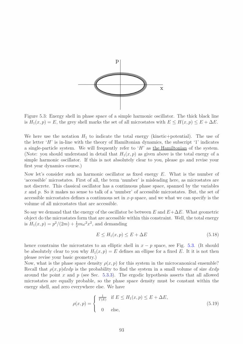
Figure 5.3: Energy shell in phase space of a simple harmonic oscillator. The thick black lineis H1(x, p) = E, the grey shell marks the set of all microstates with E ≤ H(x, p) ≤ E +∆E.

We here use the notation H1 to indicate the total energy (kinetic+potential). The use ofthe letter ‘H ’ is in-line with the theory of Hamiltonian dynamics, the subscript ‘1’ indicatesa single-particle system. We will frequently refer to ‘H ’ as the Hamiltonian of the system.(Note: you should understand in detail that H1(x, p) as given above is the total energy of asimple harmonic oscillator. If this is not absolutely clear to you, please go and revise yourfirst year dynamics course.)

Now let’s consider such an harmonic oscillator as fixed energy E. What is the number of‘accessible’ microstates. First of all, the term ‘number’ is misleading here, as microstates arenot discrete. This classical oscillator has a continuous phase space, spanned by the variablesx and p. So it makes no sense to talk of a ‘number’ of accessible microstates. But, the set ofaccessible microstates defines a continuous set in x-p space, and we what we can specify is thevolume of all microstates that are accessible.

So say we demand that the energy of the oscillator be between E and E+∆E. What geometricobject do the microstates form that are accessible within this constraint. Well, the total energyis H1(x, p) = p2/(2m) + 1

2mω2x2, and demanding

E ≤ H1(x, p) ≤ E +∆E (5.18)

hence constrains the microstates to an elliptic shell in x − p space, see Fig. 5.3. (It shouldbe absolutely clear to you why H1(x, p) = E defines an ellipse for a fixed E. It it is not thenplease revise your basic geometry.)Now, what is the phase space density ρ(x, p) for this system in the microcanonical ensemble?Recall that ρ(x, p)dxdp is the probability to find the system in a small volume of size dxdparound the point x and p (see Sec. 5.3.3). The ergodic hypothesis asserts that all allowedmicrostates are equally probable, so the phase space density must be constant within theenergy shell, and zero everywhere else. We have

ρ(x, p) =

1Γ(E)

if E ≤ H1(x, p) ≤ E +∆E,

0 else,

(5.19)

93

where the quantity Γ(E) is the volume of the energy shell around E in x− p space, i.e.

Γ(E) =∫ ∫

E≤H1(x,p)≤E+∆E1 dxdp (5.20)

[Refs.: (1) Mandl 2.1-2.2; (2) Bowley and Sanchez 4.1]

5.5 The statistical basis of entropy

We are now in a position to make a connection between the microscopic world, and the secondlaw of thermodynamics. Now that we have introduced the concept of a set of microstatescorresponding to a given macrostate, we can re-formulate the second law as follows:

Re-formulation of the second law:The macroscopic equilibrium of an isolated system is the macrostate with the highest numberof microstates. Given the ergodic hypothesis, it is the most likely macrostate to be observed.

Example:Consider a system of N fair dice. For starters let us just consider N = 2. There are 36possible microstates, (1, 1), (1, 2), . . . , (5, 6), (6, 6), and if the two dice are thrown each of these36 states appears with the same probability, pi = 1/36. When we talk about macrostates,we are not interested in the outcome for each die, but only in the bulk result, for examplethe sum of the two numbers. These will be in the range from 2 to 12. Which one of these11 macrostates is the most likely one? Well, it is the one with a sum of 7, as there are 6microstates corresponding to a sum of 7. For comparison there is only one microstate thatcorresponds to a sum one 2, and similarly only one microstate corresponding to macrostate12.

Now consider a system of N dice. There will then be 6N microstates, and the macrostate withthe most microstates will be the one with a sum of 3.5N . If you shake a big bag of a largenumber of dice, the most likely sum of numbers is 3.5N . In fact if N is very large, this willbe the outcome by an overwhelming probability.

See also http://people.virginia.edu/~lz2n/mse305/notes/StatThermo.pdf.

Statistical interpretation of the spontaneous increase of entropy:In earlier chapters we have seen that spontaneous processes in isolated systems (for examplefollowing the removal of constraints) lead to an increase in entropy. We can now interpret thismicroscopically. The system will initially be in the macrostate corresponding to the highestnumber of accessible microstates. ‘Accessible’ here means accessible in the situation beforethe constraints are lifted. When the constraints are removed, additional microstates becomeaccessible, and the system reacts. It’s macrostate will change and the new macrostate willbe the one with the highest number of accessible microstates after the constraints have beenremoved. It is clear that this new number of accessible microstates must be higher than thenumber of microstates that were accessible before the constraint is removed.

We can now provide a statistical basis of entropy.

Boltzmann’s definition of entropy:The entropy of the macrostate of a thermodynamic system is proportional to the logarithmof the number of accessible microstates that correspond to this macrostate:

S = k ln Ω. (5.21)

94

The quantity k is, for the moment, just an arbitrary constant, with units of energy per Kelvin.We will later see why it is the same Boltzmann constant appearing for example in the idealgas equation, PV = NkBT (where N is the number of particles, not moles).

Motivation for the logarithm:You may ask why S is proportional to the logarithm of the number of accessible microstates,and not simply equal to Ω. The reasoning is simple. We want entropy to be additive, i.e. ifwe combine two separate systems into one, we want S = S1+S2. If the number of microstatesaccessible by the first system is Ω1, and that by system 2 is Ω2, then the combined systemwill have Ω = Ω1Ω2 microstates. Hence S ∝ lnΩ is a sensible definition.

The second law of thermodynamics has become a statistical statement: Classically, the sys-tem is evolving from a macrostate of lower entropy to one of higher entropy. Statistically, itis evolving from less probable to more probable macrostates, that is from macrostates cor-responding to smaller numbers of microstates to those corresponding to larger numbers ofmicrostates.

Note:The Boltzmann constant, kB, has dimension of entropy. One has kB = R/NA ≈ 1.381× 10−23

J K−1 ≈ 8.617× 10−5 eV K−1. kBT ≈ 140

eV for T = 300 K, room temperature.)

Together with the thermodynamic relations involving entropy S = S(E, V,N) discussed ear-lier, we now have the following basis for the statistical mechanics of isolated systems:

S = kB ln Ω, (5.22)

whereΩ = Ω(E, V,N) (5.23)

is the total number of microstates of the system consistent with a given macrostate (E, V,N).Other thermodynamic quantities are calculated using the relations derived from the funda-mental thermodynamic relations, e.g.,

1

T=

(∂S

∂E

)

V,N

P

T=

(∂S

∂V

)

E,N

. (5.24)

The first one of these is the equation E = E(T, V ) for the internal energy, and the secondrelation gives the equation of state.Therefore, the key to the microcanonical ensemble approach, i.e., to the statistical physics ofisolated systems, is to find the statistical weight Ω(E, V,N). All other physical properties canthen be obtained via the above relations.

We will apply this approach to paramagnet of spin-1/2 system in Sec. 5.6, where it is relativeeasy to count the statistical weight Ω(E, V,N). Furthermore, the second relation in Eq. (5.24)gives a precise definition of temperature for an isolated system, from microscopic point of view,namely, if we can find the statistical weight Ω(E, V,N) of the system as a function of its energy,then we can find its temperature.

[Refs.: (1) Mandl 2.3; (2) Bowley and Sanchez 4.1, 4.5.]

95

5.6 Example the ideal spin-half paramagnet

5.6.1 Simple model - basic setup

We will now try to evaluate Ω for a simple model system. Hence, the corresponding physicsessentially becomes a counting problem. Consider a system of the following type: (i) con-stituents are localised at fixed sites (e.g., crystalline solids); (ii) the particles are assumed tobe independent (i.e., they not to interact with each other); (iii) each particle has a set ofenergy levels ǫ0, ǫ1, ǫ2, · · · .The most basic scenario is a system, in which each particle has just two energy levels, e.g., theideal spin-1/2 paramagnet. Paramagnetism arises when some of the atoms in a crystal havea resultant magnetic dipole moment, associated with electron orbital angular momentum orelectron spin (or both).Spins reside at the sites of a lattice, at each of N sites we have an atom with spin S = 1/2.According to quantum mechanics, the z-component of each spin has only two possible values:Sz = −1/2 for the down-state (↓) and Sz = 1/2 for the up-state (↑). Each spin has a magneticmoment −µ (↓) or µ (↑). It is here important not to confuse the magnetic moment, µ, withthe chemical potential, also µ. The total magnetic moment of the system is then

m = n↑µ+ n↓(−µ) = (n↑ − n↓)µ = (2n↑ −N)µ (5.25)

where n↑ = number of spin-up atoms and n↓ = number of spin-down atoms. Obviously,n↑ + n↓ = N .We will neglect interaction between the spins. In an external magnetic field B the energy ofa magnetic dipole µ is −µ · B (see e.g. Grant and Phillipps). Hence, in our case the totalenergy of the system is

E = n↑(−µB) + n↓(µB) = −(2n↑ −N)µB = −mB. (5.26)

5.6.2 Microstates and macrostates

Macrostates for this system can be characterized by their total magnetic moment m (i.e.,equivalently by the number of up-spins, see Eq. (5.25)). In order to specify a microstate, onthe other hand, we have to know the state (up/down) of each and every spin.

For N = 3 we have 4 macrostates (you should understand why) and 23 = 8 microstates (youshould understand why). They are the following:

m = 3µ ↑↑↑m = µ ↑↑↓, ↑↓↑, ↓↑↑m = −µ ↑↓↓, ↓↑↓, ↓↓↑m = −3µ ↓↓↓

So we have Ω(m = 3µ) = Ω(m = −3µ) = 1, and Ω(m = µ) = Ω(m = −µ) = 3.

More generally, we can ask how many microstates there are for a given macrostate for a systemof N spins. Such a system will have 2N microstates in total, but they correspond to differentmacrostates. So we ask:

96

Question:How many microstates for a given macrostate (N, n↑)?

Answer:We have to choose n↑ objects out of a total of N objects, there are

Ω(N, n↑) =N !

n↑!(N − n↑)!(5.27)

possibilities to do this. This is the number of microstates of given n↑, i.e. the number ofmicrostates corresponding to the macrostate (N, n↑). If we sum over all n↑ we must recoverthe total number of microstates, 2N , of this system. If we don’t, then we have made a mistake.So let’s check:

N∑

n↑=0

Ω(N, n↑) =N∑

n↑

N !

n↑!(N − n↑)!= 2N . (5.28)

Phew. You should by the way understand the last equal sign in this calculation, if you do not,then you need to revise the binomial expansion1.

The quantity Ω(N, n) is shown as a function of n/N for different N in Fig. 5.4, normalized to1 at the peak. See also Example Sheets 7 and 8.

Example:Suppose we have N = 1023 spins, and a total energy of E = 0 in an external magnetic field,B 6= 0. How many accessible microstates are there?

Answer:The macrostate is one with zero total energy, so half of the spins must be in the ‘up’ state, theother half in the ‘down’ state. So n↑ = N/2. The number of accessible microstates is hence

Ω(E = 0, B,N = 1023)) =N !

[(N/2)!]2≈ 103×1022 forN = 1023. (5.29)

Compare: Number of protons and neutrons in the Universe: ∼ 1080.

5.6.3 Stirling approximation

Before we continue, let us introduce an important approximation, frequently used in thecontext of counting microstates.

Stirling approximation:For large enough n we have

n! =√2πnnne−n

[1 +

1

12n+ . . .

], valid for n≫ 1. (5.30)

In logarithmic form this can be written as

lnn! ≈ n lnn− n+1

2ln(2πn) + . . . (5.31)

1I realise that I have been saying ‘You should understand the equal sign in Eq. (. . . )’ on several occasionsnow. Generally, you should make sure that you understand every equal sign in these lecture notes.

97

Figure 5.4: Number of microstates in a paramagnet with N spins, as a function of the re-scalednumber of up-spins, n/N (n = n↑). Curves are normalised to 1 at the peak.

[If you check this carefully, I have already ignored the 1/(12n) term in the above directrepresentation]. In textbooks you will also find lnn! ≈ n lnn − n, with the ln(2πn)-termomitted. This makes sense in the limit of large n, as lnn is then much smaller than n orn lnn. It really depends on how accurately you want to approximate the factorial, i.e. howmany orders of sub-leading terms you want to include.

5.6.4 Paramagnet - the thermodynamic limit

Back to the problem with the paramagnet. Let us consider B = 0 (zero external magneticfield). In this case all microstates have the same energy (zero) and, following the ergodichypothesis, they are equally likely. This is just like our checkerboard example in Sec. 5.2. Wecan ask

Question:If we take a ‘photograph’ of the system at a random time, how likely is it to observe a giventotal magnetisation, m (equivalently, a given number of up-spins, n↑)?

Answer:

Given that all 2Nmicrostates are equally likely in absence of an external field, the probabilityto find the system in a state with exactly n↑ up-spins is Ω(N, n↑)/2

N . So we need to studythe shape of Ω(N, n) as a function of n.

Crude argument (thermodynamic limit for beginners):In order to determine the shape of Ω(N, n) it is best to consider the logarithm

lnΩ(N, n) = ln(N !)− ln(n!)− ln[(N − n)!]. (5.32)

98

Let us look at Ωmax = Ω(N,N/2). We use the Stirling approximation to arrive at

lnΩmax = lnΩ(N,N/2) = ln

[N !

[(N/2)!]2

]

≈ N lnN −N − 2[N

2lnN

2− N

2

]= N ln 2. (5.33)

You should make sure you understand each and every equal sign in this expression.

This means that Ω(N,N/2) ≈ 2N , i.e. all 2N microstates are concentrated around n = N/2.So if you pick one of the 2N microstates at random, you will with overwhelming probabilityhave picked one with n↑ = N/2 up-spins, i.e. a state in which half of the spins are up, andthe other half down.

Important: This is not because these microstates are favoured in any way, it is just becausethey outnumber all other states by a huge margin.

To say the same thing in different words, look at the following inequalities (you should under-stand why each of the ‘<’ holds):

Ω(N,N/2) < Ω(N) < N · Ω(N,N/2). (5.34)

Since all terms are positive, we can take logs

lnΩ(N,N/2) < ln Ω(N) < ln Ω(N,N/2) + lnN (5.35)

But lnN ≪ lnΩ(N,N/2) ≈ N ln 2 (because of N ≫ lnN), hence lnΩ(N) is ‘squeezed’ bylnΩ(N,N/2) from below and from above, so it must be approximated by it in the limit N ≫ 1:

lnΩ(N) ≈ ln Ω(N,N/2). (5.36)

These result mean that the average over all microstates can be replaced by only looking atthose with n = N/2. In the sum over all microstates, you only have to consider those withn = N/2. It is quite common in statistical mechanics to find such examples where sums can,to a very good approximation, be replaced by their largest term - it is always a consequence(as here) of the very sharply peaked nature of the function in the sum.

More refined argument (thermodynamic limit for professionals):A more refined argument can be developed as follows. As N increases the function Ω(N, n) ismore and more sharply peaked around its maximum at n = N/2 , see Fig. 5.4. In the limitN ≫ 1 the curve is very well approximated by a Gaussian

Ω(N, n) ≈√

2

πN2N exp

[−(n−N/2)2

N/2

], N ≫ 1, (5.37)

as the keen and ambitious will show in a challenge question on example sheet 7 (the proof isagain based on the Stirling approximation). Recall the standard Gaussian

ρ(x) =1√2πσ2

e−(x−〈x〉)2/(2σ2). (5.38)

99

So we here have 〈n〉 = N/2 and σ =√N/2 and σ/n = 1/

√N , namely, relative magnitude of

fluctuations is proportional to 1/√N , a standard result for large systems 2. As N increases

the curve will be more and more sharply peaked around the maximum. In fact the peak isreally very very sharp for realistic system sizes. For example, for a macroscopic sample withN = 1024 we have σ/ 〈n〉 = 10−12.

So we see that for macroscopic systems, the macroscopic (thermodynamic) properties areextremely sharply defined, all you will ever see is the most likely behaviour, which occurs withoverwhelming probability. Statistical fluctuations are so rare that they are imperceptible.Next, we discuss the thermodynamics of spin paramagnet using the statistical mechanicsformulas discussed earlier.

5.6.5 The thermodynamics of the isolated ideal spin-1/2 paramag-

net in an external magnetic field

We now consider the case B 6= 0. The key question is to determine the internal energy andmagnetization as a function of temperature.In this case the work term dW = −PdV is replaced by dW = −mdB. The fundamentalthermodynamic relation is

dE = TdS −mdB (5.39)

or

dS =1

TdE +

m

TdB. (5.40)

Hence, once we have computed S = S(E,B,N), we can use with

(∂S

∂E

)

B,N

=1

T,

(∂S

∂B

)

E,N

=m

T. (5.41)

to find the temperature and total magnetisation,m. This is the thermodynamic magnetisation,so the average over all accessible microstates.Now, if the system is isolated, E is fixed, and hence, since E = (N − 2n↑)µB from Eq. (5.26),n↑ is fixed. The number of accessible microstates at fixed energy is hence Ω = Ω(n↑, B,N),and so the Boltzmann entropy is

S(E(n↑), B,N) = kB ln Ω(n↑, B,N)) = kB ln

[N !

n↑!(N − n↑)!

](5.42)

with

n↑ =1

2

(N − E

µB

). (5.43)

We use the Stirling approximation again to for lnN !, lnn!, ln(N − n)!, and find

S = kB

N lnN −N − [n↑ lnn↑ − n↑]− [(N − n↑) ln(N − n↑)− (N − n↑)]

, (5.44)

i.e.,S = kB[N lnN − n↑ lnn↑ − (N − n↑) ln(N − n↑)]. (5.45)

2The N−1/2 behaviour is ultimately a consequence of the central limit theorem.

100

Temperature:We find

1

T=

(∂S

∂E

)

B,N

=

(∂S

∂n↑

)

N

(∂n↑

∂E

)

B,N

, (5.46)

which reduces to1

T= kB[− lnn↑ − 1 + ln(N − n↑) + 1]

(− 1

2µB

), (5.47)

i.e.,1

T=

kB2µB

lnn↑

n↓, (5.48)

where n↓ = N − n↑.

A few interesting observations:

• We always have T > 0 since n↑ > n↓ (there will always be more spins aligned along Bthan against it);

• T = ∞ for n↑ = n↓;

• T = 0 for n↓ = 0.

• We can solve for Using the fact that N = n↑ + n↓ we can find say n↑ as a function ofT from Eq. (5.48). We can then use Eq. (5.26) to find the energy E as a function oftemperature:

E = −NµB tanhµB

kBT. (5.49)

For details, see Example Sheet 8.

Magnetisation:We also find

m

T=

(∂S

∂B

)

E,N

=

(∂S

∂n↑

)

N

(∂n↑

∂B

)

E,N

, (5.50)

and hencem

T= kB[− lnn↑ + ln(N − n↑)]

(E

2µB2

), (5.51)

orm

T= − kBE

2µB2lnn↑

n↓. (5.52)

Combining this with Eq. (5.48) we find

m = − kbE

2µB2· 2µBkB = −E

B, or E = −mB, (5.53)

as required.

Important remark:As discussed above we obtain the energy as a function of T in explicit form for this example(you will work this out on problem sheet 8). Together with E = −mB, this gives us themagnetic moment, m, as a function of T . This is a remarkable result, derived from firstprinciples (Boltzmann entropy), it produces an actual quantitative prediction. Recall thatwe said that thermodynamics does not generate specific numbers, but only relations betweenquantities.

101

5.7 Information entropy and the principle of maximal

ignorance

5.7.1 The method of Lagrange multipliers

We follow the book by Boas (Mathematical methods in the physical sciences), Sec. 9.

Often one has to solve maximisation (or minimisation) problems with constraints. Take thefollowing example:

Maximise the function f(x, y) = (x− y)2 under the constraint x2 + y2 = 1.

Here, the variables, x and y are coupled through the constraint x2 + y2 = 1, they are notindependent.

For this particular example, we can use a trick. We can write x = cos t and y = sin t, theconstraint is then automatically fulfilled. We then only need to worry about the minimisationof f , written as a parametric function of t:

g(t) ≡ f(x(t), y(t)) = (cos t− sin t)2 = 1− 2 sin t cos t. (5.54)

The extremisation is then easy, take dg/dt = 0, and find

−2(cos t)2 + 2(sin t)2 = 0, (5.55)

i.e. cos t = ± sin t. Using x = cos t and y = sin t, we find that the extrema occur at the fourpoints (x, y) = (±1/

√2,±1/

√2). Of these two are maxima, and two are minima, and it is

easy to work out which are which (can you do that?).

But, in this example we are lucky, we were able to express x and y in parametric form as afunction of t. This was because the constraint had a very special form (the unit circle). Whatdo we do for less convenient constraints?

General problem: Find the maximum (or minimum) values of the function f(x, y) when x andy are related by the constraint φ(x, y) = 0.

Solution:Given that x and y are related through the constraint, the function f is really only a functionof one of the two variables, say x. To find extrema we have to set df/dx = 0, i.e. df = 0. Thiscan be written as

df =

(∂f

∂x

)

y

dx+

(∂f

∂y

)

x

dy = 0. (5.56)

The quantities dx and dy are here not independent due to the constraint. In fact given thatφ(x, y) = 0 we have

dφ =

(∂φ

∂x

)

y

dx+

(∂φ

∂y

)

x

dy = 0 (5.57)

Multiplying both sides of Eq. (5.57) by λ and subtracting this from Eq. (5.56) we have

(∂f

∂x

)

y

+ λ

(∂φ

∂x

)

y

dx+

[(∂f

∂y

)

x

+ λ

(∂φ

∂y

)

x

]dy = 0 (5.58)

102

This is true for all λ, so we can choose λ as we wish. Specifically we will make the choice

λ = −( ∂f

∂y )x( ∂φ

∂y )x. Then we get

(∂f

∂x

)

y

+ λ

(∂φ

∂x

)

y

= 0,

(∂f

∂y

)

x

+ λ

(∂φ

∂y

)

x

= 0. (5.59)

These two equations can now be solved, together with φ(x, y) = 0 to give x, y and λ.

Example:Let’s take our example from above. We have f(x, y) = (x− y)2 and φ(x, y) = x2 + y2 − 1. Sothe two equations in (5.59) read

2(x− y) + 2λx = 0

−2(x− y) + 2λy = 0. (5.60)

Subtracting these off each other gives

(x− y)(2 + λ) = 0, (5.61)

i.e. x = y, or λ = −2. For λ = −2 we conclude 2(x− y)− 4x = 0 (using 2(x− y) + 2λx = 0),i.e. −2(x+ y) = 0, so x = −y. So again we find x = ±y, and the constraint x2 + y2 = 1 leadsto the same four points as above, i.e,.

(1/√2, 1/

√2), (−1/

√2,−1/

√2), (1/

√2,−1/

√2), (−1/

√2, 1/

√2). (5.62)

Two of these are maxima, the other two minima.

Remark:The above equations (5.59) are exactly the equations we obtain if we construct the function

F (x, y, λ) = f(x, y) + λφ(x, y), (5.63)

with two independent variables x and y, and if we then extremise this with respect to x, yand λ (the extermination with respect to λ gives ∂λF (x, y, λ) = 0, i.e. φ(x, y) = 0, so exactlythe constraint subject to which we optimise x and y.)

The variable λ is called the Lagrange multiplier.

This can be generalised to problems with multiple variables, x1, x2, . . . , xM :

Method of Lagrange multipliers:To find the minimum (or maximum) values of f(x1, x2, . . .) when x1, x2, . . . are related by aconstraint φ(x1, x2, . . .) = 0 construct the function

F (x1, x2, . . . , xM , λ) = f(x1, . . . , xM) + λφ(x1, . . . , xM) (5.64)

and set all partial derivatives to zero

∂F

∂x1=∂F

∂x2= . . . =

∂F

∂xM= 0. (5.65)

Solve these equations together with the constraint φ(x1, . . . , xM) = 0 to get x1, . . . , xM .

103

5.7.2 Shannon entropy

Consider the situation in which one of M events may occur, label them i = 1, . . . ,M . Eachevent, i, happens with known probability pi, where

∑i pi = 1. Until one of the event actually

happens, the information provided by the occurrence of the event is missing. We will call thisthe ‘missing information’.Now, how much information do we gain, when an event actually happens? Say the eventoccurs with a high probability, it is a frequent event. The occurrence of such an event willprovide only a relatively small amount of information (say ‘rain in Manchester’). The extremecase is an event that occurs with absolute certainty (pi = 1), for example ‘England beatenby Germany in football penalty shoot-out’. The actual occurrence of such an event providesno information at all, since we knew from that start that this would happen. A rare eventhowever provides a non-zero amount of information.

Let us formalise this. We wish to define a measure I(p) of the information we gain when anevent which occurs with probability p actually occurs. We require the following properties ofI(·):

• It has to be monotonic, the information gained from the occurrence of an event increasesthe less frequent the event is: I(p2) > I(p1) if p2 < p1.

• I(p) is a continuous function of p, it is non-negative (i.e., I(p) ≥ 0) and we have I(p =1) = 0 (no information gained if the event is certain).

• The probability that two indistinct events i and j happen independently is pipj , and theinformation gained by this needs to be equal to the sum of information gained by eachof the two events. I.e., we require I(p1p2) = I(p1) + I(p2).

It turns out that, up to an overall multiplicative factor, the only mathematical function withthese properties is the negative logarithm, so we define the ‘missing information’ of an eventwhich occurs with probability pi as

I(pi) = − ln pi. (5.66)

The average information provided by an event is then given by by the average over all events,i.e. by the so-called

Shannon entropy:

I(p) = −∑

i

pi ln pi. (5.67)

5.7.3 The microcanonical ensemble

We can now return back to the micro canonical ensemble, and the principle of equal a-prioriprobabilities. It can be derived from the following

Principle of maximum Gibbs entropy:For a given set of constraints let pi be the probability that a thermodynamic system is found

104

in the accessible microstate i. The pi are then such as to maximise the Gibbs entropy3

S = −kB∑

i

pi ln pi. (5.68)

Application to the micro canonical ensemble:Let us consider an isolated thermodynamic system. If we restrict the allowed states i =1, . . . ,Ω to those with the given energy, we have no constraints on the pi other than

∑Ωi=1 pi =

1. So we have the following maximisation problem:

Maximise S = −kB∑

i pi ln pi under the constraint∑

i pi = 1.

We solve this using the method of Lagrange multipliers. The constraint can be written asφ(p1, p2, . . .) = 0, if we introduce φ(p1, p2, . . .) =

∑i pi − 1. So we construct

F (p1, p2, . . . , λ) = −∑

i

pi ln pi + λ

(∑

i

pi − 1

)(5.69)

Taking ∂F∂pj

for a fixed j gives

−kB ln pj − kB + λ = 0 (5.70)

[To understand this, consider a concrete value of j, say j = 3. In the above sums over iyou can then ignore all terms other than the one with i = 3. We have used the fact thatddp[p ln p] = ln p+ p× (1/p) = ln p+ 1.]

From Eq. (5.70) we conclude that pj = exp((λ/kB)− 1) for all j, i.e. in particular that all pjmust be identical. Given the normalisation, this leaves

pj =1

Ω(5.71)

for all j = 1, . . . ,Ω. This is of course the micro canonical ensemble as we have discussed itabove.

So we have shown that the principle of equal a-priori probabilities over accessible microstatesfollows from the principle of maximum ‘missing information’ (or maximum uncertainty). Ifwe know nothing about the probability distribution over allowed microstates other than thatit is normalised, then the distribution which maximises the uncertainty is that of the micro-canonical ensemble.

Nice, innit?

3Compared to the Shannon entropy the Gibbs entropy contains an additional factor kB. The Shannonentropy comes from information theory, and has no relation to thermodynamics. It is dimensionless. TheBoltzmann constant in the Gibbs entropy is required to make the Gibbs entropy, obtained from maximisationas explained in the text, agree with the thermodynamic entropy. Given that both entropies only differ by aconstant factor, it does not make a difference which one of the two one maximises. If one is maximised so isthe other.

105

5.8 Density of states and correspondence between clas-

sical and quantum mechanical statistical weight

As discussed in Sec. 5.5, the Boltzmann entropy relies on a counting of the microstatesaccessible by a given system. A microstate of a quantum system is specified by a set ofdiscrete quantum numbers. Therefore, in principle, there is no ambiguity in counting thetotal number of the microstates Ω in Quantum Mechanics. We have seen an example in Sec.5.6, where we have counted the microstates explicitly.In a classical system, the same can not be said as a microstate is specified by the continuousvariables ri, pi, i = 1, 2, · · · , N . So it is not clear how to ‘count’ microstates, and how to definethe Boltzmann entropy.

We will now try to resolve this issue.

5.8.1 Qualitative argument:

A classical state (r, p) makes no sense quantum-mechanically, as position and momentumcannot be specified sharply simultaneously. The uncertainty principle imposes the limit

∆x∆px ≥ h

2, (5.72)

and similarly for the other components.This suggests that each microstate takes requires a phase space volume proportional to h3,one factor of h for each dimension. Each microstate effectively corresponds to a cell of a sizeproportional to h3 in phase space. A more detailed analysis of simple model systems (seebelow) shows that the precise phase space volume is given by h3, where

h = 6.626× 10−34 m2 kg s−1, (5.73)

is Planck’s constant.This defines a unique correspondence between the classical and quantum mechanical calcula-tions of the total number of the microstates Ω.

For a single particle the ‘number’ of accessible microstates is hence

Ω =1

h3

∫d3rd3p, (5.74)

whered3p = dpxdpydpz, (5.75)

where where the integral is over the volume in phase space allowed within externally appliedconstraints. In the example of the harmonic oscillator, this could be a given energy shell, seeEq. (5.20).

5.8.2 Quantum mechanical density of states

Let us consider a single quantum particle confined to the space 0 ≤ x ≤ L, i.e. a box withsides of length L. The stationary Schrodinger equation then reads

− h2

2m

∂2

∂x2Ψ(x) = 0, (5.76)

106

for 0 ≤ x ≤ L. Following e.g. Mandl (see appendix B) or indeed the Ashcroft and Merminbook on solid state physics we apply periodic boundary conditions, i.e. Ψ(x + L) = Ψ(x).This makes it possible to consider travelling wave solutions. Solutions are of the form

Ψ(x) = A exp(ikx) (5.77)

where k = 2πLn, and where n = 0,±1,±2, . . . is the corresponding quantum number. The above

wave functions (plane wave solutions) are the eigenfunctions of the momentum operator. Thequantum mechanical momentum of these eigenfunctions (of the momentum operator) is givenby

p = hk =h

Lnx, (5.78)

where h = 2πh. On the p-line these states are lined up in sequential order with a distance ofh/L. The number of these states within a momentum interval ∆p is hence given by L∆p/h,so one state per L∆p/h.

Going to three dimensions, the number of quantum states within a phase space volumeLxLyLz∆px∆py∆pz is hence Lx∆px

h× Ly∆py

h× Lz∆pz

h. This motivates the above statement

Ω =1

h3

∫d3xd3p. (5.79)

A very similar argument can be derived from the usual boundary condition, Ψ(x = 0) = Ψ(x =L) = 0, for a quantum particle in a potential well (with infinite potential outside the box).See e.g. this set of notes here http://www.sfu.ca/~boal/445lecs/445lec24.pdf. This canalso be found in various textbooks, see again Mandl for example.

You can find more on the density of states in quantum systems in the Britney Spears guideto semiconductor physics:

http://britneyspears.ac/physics/dos/dos.htm

[Refs.: (1) Mandl 2.4; Mandl, Appendix B; (2) Bowley and Sanchez 2.9.]

107

Chapter 6

The statistical physics of non-isolatedsystems: Boltzmann distribution andcanonical ensemble

“His line of thought may be called my first love in science. No other has ever thusenruptured me or will ever do so again.”(Erwin Schrodinger about Boltzmann)

“I don’t believe that atoms exist!”“Have you seen one?”(Ernst Mach)

“Whoever rejects faith in the reality of atoms . . . will find it difficult to advancephysical knowledge.”(Max Planck)

6.1 Recap: constant-energy distribution (a.k.a. micro-

canonical ensemble)

This distribution applies to isolated systems, E, V,N fixed. In practice we assume that theenergy lies in the range E to E+ δE. The system is isolated, so the postulate of equal a-priorprobabilities can be directly applied: system equally likely to be found in any of its accessiblemicrostates:

pi =

1Ω

if E < Ei < E +∆E,

0 else,(6.1)

where Ω is the statistical weight of the macrostate specified by E, V,N .

This is the constant energy (or microcanonical) distribution.

Disadvantage:Inconvenient for calculations, not very flexible.

But, very useful as a starting point for deriving the Boltzmann distribution.

108

Figure 6.1: Construction used to derive the Boltzmann distribution.

6.2 Derivation of the Boltzmann distribution

Consider a system S in contact with a heat reservoir R at temperature T as shown in Fig.6.1. The system and the reservoir together(‘R+S’), form an isolated system with fixed energyE0. Heat can be exchanged between S and R, but R is so large that its temperature remainsT if heat is exchanged. We now ask: What is the probability pi that the system S is in aparticular microstate with energy Ei?The total number of microstates of the combined system is

Ω = ΩR × ΩS. (6.2)

Now, let us consider a specific microstate i of the system S, and say that S has energy Ei inthat state. How many microstates of the combined system are now accessible? Well, the stateof S has been fixed, but R can take any of its microstates, provided that that R has energyE0 − Ei. Recall that the combined system is isolated and has total energy E0, and we havefixed that of S to be Ei.So the number of accessible microstates of the combined system is now

Ω = ΩR(E0 − Ei)× 1, (6.3)

where ΩR(E0 −Ei) is the number of microstates of the reservoir with energy E0 − Ei.

Thus, the probability pi of S being in a state with energy Ei depends on the number ofmicrostates of R with energy E0 − Ei,

pi = pi(Ei) =ΩR(E0 −Ei)

ΩR+S(E0)=

number of microstates of (S +R) withS in state i

total number of microstates of (S +R). (6.4)

Now, use the Boltzmann relation S = kB ln Ω from the previous chapter:

ΩR(E0 −Ei) = exp[1

kBSR(E0 − Ei)

]. (6.5)

If R is a good reservoir it must be much bigger than S, so Ei ≪ E0. So, let’s Taylor expandaround E0:

SR(E0 −Ei) = SR(E0)− Ei

(∂SR

∂E

)

V,N

E=E0

+ · · · . (6.6)

109

But, from the thermodynamic relations involving partial derivative of S,,(∂SR

∂E

)

V,N

=1

T. (6.7)

Thus,

SR(E0 −Ei) = SR(E0)−Ei

T+ . . . . (6.8)

This gives

pi ∝ ΩR(E0 −Ei) = exp[1

kBSR(E0 − Ei)

]≈ exp

[SR(E0)

kB− Ei

kBT

], (6.9)

i.e. we have foundpi = const.× e−Ei/(kBT ). (6.10)

We have used that SR(E0) is a constant, independent of the microstate i of the system S. The

constant in Eq. (6.10) is labeled 1/Z by convention, i.e.

pi =1

Ze−Ei/(kBT ). (6.11)

The quantity Z is then determined from the overall normalisation, all microstates∑

i

pi = 1. (6.12)

This meansZ =

∑

i

e−Ei/(kBT ), (6.13)

where sum on i runs over all distinct microstates i of the system S.

We have thus derived the

Boltzmann distribution

pi =1

Ze−Ei/(kBT ), Z =

∑

i

e−Ei/(kBT ). (6.14)

The quantity Z is called the partition function of the system S (Boltzmann called this ‘Zus-tandssumme’ in German, roughly ‘sum over states’, hence the letter Z). As we will see later,partition function Z is very useful because all other thermodynamic quantities can be calcu-lated through it. Keep in mind that Z = Z(T, V,N) is a function in particular of temperature.

Remark:The Boltzmann distribution gives the probability that a system, when placed in contactwith a heat reservoir at temperature T , is in a particular state. This is also known as thecanonical ensemble.

Remark 2:It is very common to introduce the notation

β =1

kBT, (6.15)

110

this is often referred to as the ‘inverse temperature’ in statistical physics. The Boltzmanndistribution then becomes

pi =1

Ze−βEi, Z =

∑

i

e−βEi . (6.16)

Remark 3 (important!):It is important to emphasize also that the index i labels the microstates of N -particles andEi is the total energy. For example, a microstate for the case of an spin-1/2 paramagnet of Nindependent particles is a configuration of N spins (up or down):

i = (↑, ↑, ↓, . . . , ↓). (6.17)

For a gas of N molecules, however, i represents a set of values of positions and momenta as

i = (r1, r2, . . . , rN;p1,p2, . . . ,pN),

as discussed in Sec. 5.2.

For (classical) systems with continuous states:

Single-particle partition function:

Z1 =∫d3rd3p

h3e−βH1(r,p) (6.18)

For an N -particles system with distinguishable particles the N -particle partition function is:

ZN =∫d3Npd3Nr

h3Ne−βHN (r

1,p

1,...,rN ,p

N). (6.19)

We will discuss the case of indistinguishable particles below.

[Ref.: (1) Mandl 2.5; (2) Bowley and Sanchez 5.1-5.2]

6.3 Derivation from maximum-entropy principle

In Sec. 5.7 we have introduced the Gibbs entropy of an ensemble

S = −kB∑

i

pi ln pi. (6.20)

We will now show that the Boltzmann distribution maximises this entropy under the constraintof a fixed average energy.

So consider the following maximisation problem:

Find the pi such that S = −kB∑

i pi ln pi is maximal, given the constraints:

(i)∑

i pi = 1 (normalisation), and

(ii)∑

i piEi = E. Here E is then given value of the average energy.

111

Solution:We use the method of Lagrange multipliers. Define

F (pi, λ1, λ2) = −kB∑

i

pi ln pi + λ1

(∑

i

pi − 1

)+ λ2

(∑

i

piEi −E

). (6.21)

Taking ∂∂pi

of this object, and setting this to zero, we find:

−kB (ln pi + 1) + λ1 + λ2Ei = 0. (6.22)

Re-arranging this gives

pi = eλ1kB

−1e

λ2EikB (6.23)

It is here important to keep in mind that λ1 and λ2 are Lagrange multipliers, they enforce theconstraint, but they do not depend on i. The quantity λ2 in the first exponential can be usedto enforce normalisation (the above constraint (i)). So we have

pi =e

λ2EikB

Z, (6.24)

where Z =∑

j eλ2EjkB . This is already looking good, as pi depends on Ei through an exponential.

It remains to relate λ2 to temperature.

To do this keep in mind that λ2 is the Lagrange multiplier enforcing∑piEi = E for the given

value of E (constraint (ii)).

Using this, we have

S = −kB∑

i

pi ln pi

= −kBZ

∑

i

eλ2Ei/kB

(λ2kBEi − lnZ

)

= −λ21

Z

∑

i

Eieλ2Ei/kB

︸ ︷︷ ︸=〈E〉

+kBZ

lnZ∑

i

eλ2Ei/kB

︸ ︷︷ ︸=Z

.

= −λ2E + kB lnZ. (6.25)

Next we use (∂S

∂E

)

V,N

=1

T(6.26)

to find the identification

−λ2 =1

T. (6.27)

Thus we have

pi =1

Ze

λ2EikB =

1

Ze−

EikBT , (6.28)

i.e. the Boltzmann distribution.

112

6.4 The partition function

Although the partition function, Z =∑

i e−βEi, is initially introduced as a relatively innocent

normalization constant, its usefulness is much deeper than that. Loosely speaking all ther-modynamic quantities of a system in thermal equilibrium at temperature T can be computedif its partition function is known, just in the same way that all thermodynamic informationof an isolated system (at fixed E,N, V ) is contained in Ω(E,N, V ). For a system in thermalequilibrium everything is know (i.e., can be derived) when Z is known. Keep in mind that thismeans Z = Z(T,N, V ) for a hydrostatic system, or Z = Z(T,N,B) for a magnetic system,etc..

Above we say that everything ‘can be derived’ once Z is known. But I haven’t told you howthis is done in practice. So here we go.

6.4.1 Expected internal energy

The expected internal energy of the system is calculated as the average 〈E〉 = ∑i piEi, i.e.

〈E〉 = 1

Z

∑

i

Eie−Ei/kBT =

∑iEie

−βEi

∑j e

−βEj(6.29)

Fact:

〈E〉 = − 1

Z

(∂Z

∂β

)

V,N

. (6.30)

Proof:

− 1

Z

(∂Z

∂β

)

V,N

= − 1

Z

∂

∂β

∑

i

e−βEi

= − 1

Z

∑

i

(−Eie

−βEi

)

=1

Z

∑

i

Eie−βEi, q.e.d. (6.31)

Exercise:Show that

〈E〉 = −(∂ lnZ

∂β

)

N,V

= kBT2

(∂ lnZ

∂T

)

N,V

. (6.32)

[You must do this in detail!]

6.4.2 Entropy

We haveS = −kB

∑

i

pi ln pi. (6.33)

113

This can either be accepted as a postulate (see the section on information theory), or youcan derive it as the entropy of an ensemble, see e.g. Mandl, Chapter 2.5. For the Boltzmanndistribution we have (repeating the same calculation we did already above):

S = −kB∑

i

pi lne−βEi

Z

= −kB∑

i

pi(−βEi − lnZ)

= kBβ∑

i

piEi + kB lnZ∑

i

pi

= kBβ〈E〉+ kB lnZ (6.34)

where we have used the definition 〈E〉 =∑

i piEi and normalization condition∑

i pi = 1.Rearrange the above equation

kBT lnZ = −(〈E〉 − TS), (6.35)

i.e.,TS = 〈E〉+ kBT lnZ. (6.36)

So if we know Z we can compute S.

6.4.3 Energy fluctuations

We have seen above how the average energy of a system can be found in the canonical ensemble:

〈E〉 = −(∂ lnZ

∂β

)

N,V

. (6.37)

From 〈E〉 we can then also calculate the heat capacity

CV =

(∂〈E〉∂T

)

N,V

= kBβ2

(∂2 lnZ

∂β2

)

N,V

. (6.38)

Make sure you understand all equalities in these expressions in detail. See also example sheet9.

The quantity 〈E〉 is the typical (‘average’) energy, but there are fluctuations as the systemmoves from one microstate to the next in the canonical ensemble. We now ask how large theseenergy fluctuations are. In fact we show that they are negligibly small in the thermodynamiclimit, N ≫ 1.

So we consider the varianceσ2 = (∆E)2 ≡ 〈E2〉 − 〈E〉2. (6.39)

Clearly

〈E2〉 =∑

iE2i e

−βEi

∑i e

−βEi=

1

Z

(∂2Z

∂β2

)

N,V

. (6.40)

(again make sure you understand all of these equal signs in detail).

114

Hence, (all derivatives in the followings are at constant N, V )

(∆E)2 =1

Z

∂2Z

∂β2−(− 1

Z

∂Z

∂β

)2

=∂

∂β

(1

Z

∂Z

∂β

)=

(∂2 lnZ

∂β2

)

N,V

= −(∂〈E〉∂β

)

N,V

= −(∂〈E〉∂T

)

N,V

dT

dβ= kBT

2〈CV 〉.

or (see also example sheet 9)

(∆E)2 =

(∂2 lnZ

∂β2

)

N,V

= kBT2CV . (6.41)

It is important that you go through this calculation step by step with a pencil and a pieceof paper, and that you understand all equalities. You should do this for all (!) calculationsin these notes. Unfortunately I know of no other way of acquiring a good and thoroughunderstanding of the material.

Remark:For a macroscopic system we typically have 〈E〉 ∝ NkBT , and CV ∝ NkB, hence

∆E

〈E〉 ∝√NkBT

NkBT=

1√N.

So, if N ≈ 1024, ∆E/〈E〉 ≈ 10−12, an unobservably tiny number! So, for most normalmacroscopic systems the fluctuations are totally negligible and we can forget the notation 〈〉,and write 〈E〉 → E, etc., and there is no real difference between an isolated system of fixedenergy E and one in contact with a heat bath at the same temperature T = (∂E/∂S)N,V .Remark:A notable exception occurs near critical points, where the distinction between two phasesdisappears. Near critical points fluctuations may not be negligible. This can sometimesbe observed as ‘critical opalescence’ where the meniscus between the liquid and gas phasesdisappears, and the mixture becomes milky-looking and opaque as it scatters light.

[Ref.: (1) Mandl 2.5]

6.4.4 The connection with thermodynamics

As discussed above, energy fluctuations are essentially negligible in macroscopic systems. Theprobability that the system has a given energy has a sharp spike at the average energy, youpractically always find that the system’s energy is equal to the average. So for all practical pur-poses the energy of a macroscopic body in contact with a heat bath is completely determined(by the temperature of that heat reservoir).

⇒ The most probable value of the energy, the mean value and the classical thermodynamicenergy are indistinguishable.

So from now on we identity the average energy, 〈E〉, with the thermodynamic energy of amacroscopic system.

From Eq. (6.35) we then haveTS = E + kBT lnZ, (6.42)

115

orF = E − TS = −kBT lnZ, (6.43)

where F ≡ E − TS is the Helmholtz free energy. Hence we have the so-called

Bridge equation:F (T, V,N) = −kBT lnZ(T, V,N). (6.44)

This equation formally makes the connection between statistical physics and thermodynamics.It is sometimes called the ‘bridge equation’, as it provides a bridge between the microscopicand the macroscopic description of a system

The other thermodynamic quantities can then calculated by partial derivatives of F , as ex-plained in the earlier chapters. We said earlier that F (T, V,N) contains the full informationabout a thermodynamic system. It is now clear that Z(T, V,N) contains the same informa-tion, hence the importance of the canonical partition function. Everything else follows bydifferentiation.

Cute observation:Compare F (T, V,N) = −kBT lnZ(T, V,N) for the canonical ensemble with S(E, V,N) =kB ln Ω(E, V,N) for the microcanonical ensemble. So the partition function, Z(T, V,N), inthe canonical ensemble is what the statistical weight, Ω(E, V,N), is in the microcanonicalensemble. Beautiful, isn’t it?

The power of going microscopic:The results we have derived provide a powerful algorithm to calculate thermal quantities forany microscopic model. If you are not impressed and amazed by this, then you probablyhaven’t understood it. Following the steps below we can derive all thermodynamic quantitiesfor any microscopic system. If you don’t find this impressive, well, then I am afraid, I can’thelp you.

• Label microstates, i, and find Ei, for example from Schrodinger’s equation.

• As a function of temperature (and V,N) calculate the partition function

Z =∑

i

e−Ei/kBT . (6.45)

• FindF = −kBT lnZ. (6.46)

• Use thermodynamics to find quantities of interest from F , e.g.,

E = −(∂ lnZN

∂β

)

N,V

= kBT2

(∂ lnZ

∂T

)

N,V

,

S = −(∂F

∂T

)

V,N

,

P = −(∂F

∂V

)

T,N

,

CV = T

(∂S

∂T

)

V,N

= −T(∂2F

∂T 2

)

V,N

,

116

µ =

(∂F

∂N

)

T,V

, (6.47)

etc etc.

Now, clearly, the difficult part is to compute Z in the first place.Remark:For magnetic systems the term −PdV is replaced by −mdB; and hence we have for examplem = −(∂F/∂B)T,N etc. instead of the above relations.

6.4.5 Further comments*

You should now be very annoyed with me!

I promised that we would derive the whole of thermodynamics again from scratch, startingfrom microscopic considerations. But in Eq. (6.7) we have introduced temperature via the

relation(∂SR

∂E

)V,N

= 1T, which we have taken from thermodynamics. That’s not nice, is it?

So let me comment on this.

Introduction of temperature

In the above derivation of the Boltzmann distribution the derivative(∂S∂E

)V,N

comes up, and

we have simply identified this with the (inverse) temperature 1Tfrom thermodynamics. But

why should this be so?

Consider again the system R+S made of a reservoir and the actual system S. The combinedsystem has energy E0, and let E be the energy of the system S alone. If the combined systemis in the macrostate defined by (E0, E) we have

ΩR+S(E0, E) = ΩR(E0 −E)× ΩS(E), (6.48)

the product of the number of states R can be in (given that R’s energy is E0 − E) times thenumber of states S can be in, given that S’s energy is E.

This expression, ΩR+S(E0, E) is a function of E, and macroscopically the observed equilibriumvalue, E∗ of E, will be such that ΩR+S(E0, E) is maximised, as maximising ΩR+S is the sameas maximising the entropy of R + S. Now at this maximum we have

∂

∂EΩR(E0 − E)ΩS(E) = 0, (6.49)

i.e.,∂ΩR(E0 − E)

∂EΩS(E) + ΩR(E0 −E)

∂ΩS(E)

∂E= 0. (6.50)

This on the other hand is the same as

−ΩRΩS

[1

ΩR(ER)

∂ΩR(ER)

∂ER− 1

ΩS(E)

∂ΩS(E)

∂E

]= 0, (6.51)

117

where we have written ER = E0 −E. From this we then conclude(∂ ln ΩR

∂ER

)

VR,NR

=

(∂ ln ΩS

∂E

)

VS ,NS

(6.52)

This relation determines E = E∗. It is the condition for thermal equilibrium derived frommicroscopic considerations. Macroscopically the condition is TR = TS.We can now formally define

β =

(∂ ln Ω

∂E

)

V,N

. (6.53)

Then the condition of thermal equilibrium between two systems 1 and 2 is β1 = β2. It isat this point clear that the quantity β =

(∂ lnΩ∂E

)V,N

must have something to do with the

temperature in classical thermodynamics. One knows from everyday experience that systemsin thermal contact equilibrate at equal temperature, and we have just shown that β1 = β2 insuch cases. But the precise connection between β and T is not clear, if we do not want to usethe thermodynamic result 1/T =

(∂S∂E

)V,N

.

We can develop the formalism of statistical mechanics with β :=(∂ lnΩ∂E

)V,N

. Following the

steps of Sec. 6.2 we can derive the Boltzmann distribution as

pi =1

Ze−βEi (6.54)

with β :=(∂ lnΩ∂E

)V,N

, based on the principle of maximising the number of accessible microstates

Ω. One does not formally have to introduce S = kB ln Ω do to this, simply write Ω = exp(lnΩ)and expand lnΩ in powers of Ei in Sec. 6.2. See also Mandl, Chapter 2.5. You arrive atpi =

1Ze−βEi with the formal definition β :=

(∂ lnΩ∂E

)V,N

.

If we then use this as a starting point and apply it to the ideal gas, we find

βPV = N, (6.55)

where N is the number of particles and where P is defined via Eq. (6.47). We will do thisderivation in Sec. 6.7.

Comparing this with PV = nRT = NkBT gives

β =1

kBT. (6.56)

We stress again that the parameter β was – in this context – introduced purely mathematicallyas β =

(∂ lnΩ∂E

)V,N

. We have to make a connection with empirical thermodynamics at some

point though and this is what we have done, we have identified β with 1/(kBT ) using theempirical behaviour of ideal gases.

This means that the connection between microscopic and macroscopic description of the worldis

1

T=

(∂kB ln Ω

∂E

)

V,N

. (6.57)

118

From classical thermodynamics we have

1

T=

(∂S

∂E

)

V,N

. (6.58)

This leads to the identification

S(E, V,N) = kB ln Ω(E, V,N) (6.59)

for a fluid.Summary:We have two routes to make the connection:

• Do as we did before: Postulate S = k ln Ω, and leave the nature of the constant kopen. Then derive the Boltzmann distribution using an expansion of S(E), and using1T=(∂S∂E

)V,N

. This delivers pi = Z−1e−Ei/(kT ), where it is not clear a-priori that k is the

Boltzmann constant. Use this, and the identification P = −kT(∂ lnZ∂V

)T,N

to study the

ideal gas, and compare with the empirically known ideal gas equation (which containskB). This leads to the identification k = kB.

• Do not introduce entropy, but derive the Boltzmann distribution using an expansion oflnΩ in E. Formally introduce β = ∂ lnΩ

∂E. This leads to pi = Z−1e−βEi. Develop the

formalism for the ideal gas using β, and compare with the empirically known ideal gasequation (which contains both T and kB). This leads to the identification β = 1/(kBT ).

Then use 1T=(∂S∂E

)V,N

from thermodynamics to make the identification S = kB ln Ω.

6.5 The independent-particle approximation: one-body

partition function

6.5.1 Systems with independent particles

We can represent a microstate of an N -particle system by specifying the microstates of allparticles, e.g.

i = (i1, i2, . . . , iN). (6.60)

This notation indicates that particle 1 is in single-particle state i1, particle 2 in state i2, etc.,(e.g., the spin configurations for a paramagnet).

If there is no interaction between the particles the total energy in the microstate of the Nparticles is then simply the sum of energies of each particle,

Ei = ǫi1 + ǫi2 + . . .+ ǫiN , (6.61)

where ǫi1 is the energy of particle 1 in state i1 etc (you should understand why this impliesthe absence of interactions). The partition function of the N -particle system then given by

Z = ZN =∑

i

e−Ei/(kBT ) =∑

i1,i2,...,iN

exp[− 1

kBT(ǫi1 + ǫi2 + . . .+ ǫiN )

]. (6.62)

119

If we further assume that N particles are distinguishable, summations over i’s are independentof one another. They can then be carried out separately as

ZN =∑

i1,i2,...,iN

e−ǫi1/(kBT )e−ǫi1/(kBT ) · · · e−ǫiN /kBT

=

∑

i1

e−ǫi1/(kBT )

∑

i2

e−ǫi2/(kBT )

· · ·

∑

iN

e−ǫiN /(kBT )

. (6.63)

It is important that you understand this step in detail. We notice that in the last equation,the summation in each factor runs over the same complete single-particle states. Therefore,they are all equal,

∑

i1

e−ǫi1/kBT =∑

i2

e−ǫi2/kBT = · · · =∑

iN

e−ǫiN /kBT .

Hence, the N -particle canonical partition function in the independent-particle approximationis,

ZN = (Z1)N , (6.64)

whereZ1 =

∑

i1

e−ǫi1/(kBT ) (6.65)

is the one-body canonical partition function.

We notice that the index i1 in the above equation labels single particle states and ǫi1 is thecorresponding energy of the single particle, contrast to the index i used in earlier sections of thischapter, where i labels the microstate of total N -particle system and ǫi is the correspondingtotal energy of the system.

6.5.2 Distinguishable and indistinguishable particles

The above analysis are valid for models of solids and paramagnets where particles are localizedhence distinguishable.

The case of N indistinguishable particles is more complicated. The fact that the permutationof any two particles in a configuration (i1, i2, . . . , iN) does not produce a new microstateimposes restrictions on the sum

∑i =

∑i1,i2,...,iN ; the number of microstates is hence much

reduced and sums over i’s are not longer independent of each other. The simple separationmethod of Eq. (6.63) is invalid.If there are N indistinguishable particles in the system, then the over counting factor is N !as there are N ! permutations for the same microstate (i1, i2, . . . , iN). For N indistinguishableparticles we hence approximate the partition function as,

ZN ≈ 1

N !(Z1)

N . (6.66)

Important remark:It is important to realise that this is an approximation. The overcounting factor of N ! onlyapplies to states in which all i1, i2, . . . , iN are pairwise different. For example if all particles arein the same one-particle microstate, i.e., i1 = i2 = . . . , iN , then there is only one permutation.

120

The above approximation hence holds only provided the number of single-particle microstatesis much larger than the number of particles. It is then very unlikely to find two particles inthe same one-particle microstate. The overcounting factor is then consistently given by N !.

Summary:

• N distinguishable particles (models of solids and paramagnets):

ZN = (Z1)N ; (6.67)

• N indistinguishable classical particles (classical ideal gas):

ZN ≈ 1

N !(Z1)

N ; (6.68)

• Either wayZ1 =

∑

i1

e−ǫi1/kBT (6.69)

is the one-body partition function, with ǫi1 the single-particle energy.

Remark:Taking the logarithm of the partition function, we have

lnZN

= N lnZ1, distinguishable particles;≈ N lnZ1 − lnN !, indistinguishable particles,

(6.70)

In both cases

E = EN = −(∂ lnZN

∂β

)

N,V

= −N(∂ lnZ1

∂β

)

N.V

= NE1, (6.71)

where E1 = −∂ lnZ1/∂β is the average energy of a single particle. Namely, in the independent-particle approximation, the total internal energy of N particles (distinguishable or indistin-guishable) is equal to N times the average energy of a single particle.

6.5.3 Example

Consider a system of two free (independent) particles. Assume that there are only two single-particle energy levels ǫ1, ǫ2. By enumerating all possible two-body microstates, determine thepartition functions Z2 if these two particle are (a) distinguishable and (b) indistinguishable.

Solution:(a) We list all four possible microstates of two distinguishable particles in the occupation diagramof Fig. 6.2.Notice that the second and third microstates are different states as two particles are distin-guishable. By definition, the partition function of the two-particle system is given by

Z2 =∑

i

e−Ei/kBT

= e−2ǫ1/kBT + 2e−(ǫ1+ǫ2)/kBT + e−2ǫ2/kBT

= (e−ǫ1/kBT + e−ǫ2/kBT )2 = Z21 , (6.72)

121

Figure 6.2: Occupation diagram of the two-particle two-level system with distinguishableparticles discussed in the text.

Figure 6.3: Occupation diagram of the two-particle two-level system with indistinguishableparticles discussed in the text.

in-line with the general expression ZN = (Z1)N of Eq. (6.67). Using Eq. (6.29) the average

energy of the two-particle system is given by

〈E〉 =1

Z

∑

i

Eie−Ei/(kBT )

=1

Z2

[(2ǫ1)e

−2ǫ1/(kBT ) + 2(ǫ1 + ǫ2)e−(ǫ1+ǫ2)/(kBT ) + (2ǫ2)e

−2ǫ2/(kBT )]. (6.73)

(b) For two indistinguishable particles, there are only three microstates as shown in Fig. 6.3.The corresponding partition function is then given by

Z2 =∑

i

e−Ei/kBT

= e−2ǫ1/kBT + e−(ǫ1+ǫ2)/kBT + e−2ǫ2/kBT . (6.74)

Notice that this partition function of two identical particles Z2 6= 12!Z2

1 as given by Eq. (7).Only the middle term has same weight as given by 1

2!Z2

1 . The average energy of the two-particlesystem is

〈E〉 = 1

Z

∑

i

Eie−Ei/kBT =

1

Z2

[(2ǫ1)e

−2ǫ1/kBT + (ǫ1 + ǫ2)e−(ǫ1+ǫ2)/kBT + (2ǫ2)e

−2ǫ2/kBT].

For the case of a two-particle system with three states, see Q1 of Example Sheet 9.

Remarks:

• It is important to note that the sum in Eq. (6.65) runs over all single-particle states i1,and not over all different energies. It is possible that different microstates have the sameenergy, i.e. a given energy level ǫi1 may be degenerate. Alternatively, we can express

122

Eq. (6.65) as a sum over distinct energy levels:

Z1 =∑

i1

e−ǫi1/(kBT )

=∑

ǫi1

g(ǫi1)e−ǫi1/(kBT ), (6.75)

where g(ǫi1) is the degeneracy factor of energy level ǫi1 .

• The one-body partition function Z1 is a useful quantity for determining N -particle par-tition function in the independent-particle approximation. However, it is important tokeep in mind that Z1 itself has no physical meaning as temperature is undefined for asingle-particle system.

• Even if we ignore interaction completely (i.e., in the independent-particle approxima-tion) and restrict to classical mechanics, many-body effects still appear for N identicalparticles as demonstrated by the 1/N ! factor.

• Eq. (6.67) is invalid in the low temperature limit where quantum effects dominate(e.g., a significant portion of particles of a quantum gas are in the zero-momentumstate: the Bose-Einstein condensation). A proper way to tackle the problems of identi-cal particles is to introduce occupation-number configurations and to use the so-calledgrandcanonical ensemble. A third-year course (Bose and Fermi gases) will discuss thissubject in detail.

[Ref.: (1) Mandl 7.1]

6.6 Further simple examples of partition function cal-

culations

In this section, we discuss a few examples of systems of non-interacting particles, and showhow to compute their partition functions.

6.6.1 The ideal spin-1/2 paramagnet

Only two energy states for each spin, i1 =↑, ↓, with energies

ǫ↑ = −µB, ǫ↓ = +µB, (6.76)

where µ is the magnetic moment of one spin particle and B is the magnetic field. The one-bodypartition function is therefore

Z1 =∑

k1

e−ǫk1/(kBT ) = eµB/(kBT ) + e−µB/(kBT ) = 2 cosh(µB/(kBT )). (6.77)

The partition function for the N spins (distinguishable particles) is

ZN = [2 cosh(µB/(kBT ))]N . (6.78)

123

6.6.2 A simple model for a one-dimensional solid

The model consists of M independent harmonic oscillators, each with energy

H1(x, p) =p2

2m+

1

2mω2x2, (6.79)

where ω is the angular frequency. The state of a classical particle is specified by i = (x, p)and the sum becomes integral

∑

i

=1

h

∫dxdp,

as discussed in Sec. 5.8.2. The one-body partition function is therefore given by

Z1 =1

h

∫dxdp e−H1(x,p)/(kBT )

=1

h

∫ ∞

−∞dpe−p2/(2mkBT )

∫ ∞

−∞dxe−mω2x2/(2kBT )

=1

h

√2πmkBT

√2πkBT

mω2

=2πkBT

hω, (6.80)

where we have used the Gaussian integral

∫ ∞

−∞e−ax2

dx =

√π

a, a > 0. (6.81)

The partition function of M oscillators (distinguishable) is

ZM = (Z1)M =

(2πkBT

hω

)M

. (6.82)

6.6.3 Classical ideal gas of N particles in a volume V

In this case, the single particle energy is

H1(r,p) = ǫ(p) =p2

2m=

1

2m(p2x + p2y + p2z). (6.83)

The one-body partition function is

Z1 =1

h3

∫d3rd3p e−βH1(p). (6.84)

As the energy ǫ(p) is r independent, the integral over real space produces a factor of volumeV and the integral over momentum is,

∫d3p e−βp2/(2m) =

(∫ ∞

−∞dpxe

−βp2x/(2m))(∫ ∞

−∞dpye

−βp2y/(2m))(∫ ∞

−∞dpze

−βp2z/(2m))

=√2πm/β ·

√2πm/β ·

√2πm/β

= (2πm/β)3/2, (6.85)

124

where we have again used the Gaussian integral formula given above. The one-body partitionfunction is

Z1 = V

(2πm/β

h2

)3/2

(6.86)

and the partition function for a classical ideal gas of N identical molecules in a volume V is

ZN =1

N !ZN

1 =V N

N !

(2πmkBT

h2

)3N/2

. (6.87)

6.6.4 Einstein model of a one-dimensional solid

Revisit the example in Sec. 6.6.2 above, but now consider the oscillators are quantum me-chanical. A single quantum oscillator has energies

ǫn = hω(n+

1

2

), n = 0, 1, 2, 3, . . . . (6.88)

The one-particle partition function is

Z1 =∑

n=0,1,2,···

e−ǫn/(kBT )

= e−hω/(2kBT )∞∑

n=0,1,2,···

e−hωn/(kBT )

= e−hω/(2kBT ) 1

1− e−hω/(kBT )

=1

2 sinh(hω/(2kT )). (6.89)

We have used the geometric series,

∞∑

n=0

xn =1

1− x, (6.90)

which you remember from primary school, and which you must remember for the rest of yourlife.

The partition function of M quantum oscillators is

ZM = (Z1)M =

1

[2 sinh(hω/2kBT )]M.

We will see later the thermodynamics of quantum oscillators reduces to the classical one inthe high temperature limit but is completely different in the low temperature limit.In the next sections, we will discuss how to calculate energy, entropy and other thermodynamicquantities from partition functions.[Ref.: (1) Mandl 2.5; (2) Bowley and Sanchez 5.1-5.2]

We have calculated the partition functions ZN for a number of very basic systems in thissection. as described above it is then straightforward to calculate other thermodynamic quan-tities. In the rest of the chapter we will do just that for a number of model systems. We willalso discuss the physical implications of our results.

[Refs.: (1) Mandl 2.5; (2) Bowley and Sanchez 5.3-5.6.]

125

6.7 Example: The classical ideal gas

Now it is time to revisit the ideal gas we discussed often in thermodynamics. We hinted beforethat it would be a challenging problem using microcanonical ensemble approach. We will showthat this is not the case using canonical ensemble approach.Note:The calculation in this section is based on a classical approach. We will repeat the samecalculation quantum mechanically in Sec. 6.8.

In Eq. (6.87) we have calculated the partition function of classical ideal gas of N identicalmolecules at fixed temperature T in a volume V

ZN =1

N !ZN

1 =V N

N !

(2πm

βh2

)3N/2

. (6.91)

Hence, using Stirling approximation, N ! ≈ (N/e)N ,

lnZN = N ln

eV

N

(2πm

βh2

)3/2 (6.92)

Now we follow the standard calculations of canonical ensemble to obtain other thermodynamicquantities. The Helmholtz free energy is obtained from Eq. (6.44)

F = − 1

βlnZN = − 1

βN

[3

2ln

(2πm

βh2

)+ ln

V

N+ 1

]. (6.93)

Note:Had we not included the 1/N ! factor in ZN , the second term in Eq. (6.93) would be lnV insteadof the intensive quantity ln(V/N) (you should convince yourself of that!), and F would not beextensive as required.

The equation of state is obtained using the definition of pressure in Eq. (6.47):

P = −(∂F

∂V

)

T,N

=1

βN · 1

V. (6.94)

With the identification β = 1kBT

we therefore obtain the familiar formula

PV = NkBT. (6.95)

The entropy is calculated using Eq. (6.47), and we find

S = −(∂F

∂T

)

V,N

= kBN

(3

2ln

2πmkBT

h2+ ln

V

N+

5

2

), (6.96)

which can be compared with Q2(a) of Example Sheet 5

S = kBN(3

2lnT

T0+ ln

V

V0

)+ const. (6.97)

126

Eq. (6.96) is referred as Sackur-Tetrode equation. It gives the absolute value of the entropy ofa gas at a given temperature T . See Q2 of Example Sheet 11 for more details. Apart from thefactor m of atomic mass, it is the same for every substance. At high enough temperature andlow enough densities all substances behave as ideal gases, and so the Sackur-Tetrode formulacan be checked experimentally. Good agreement is found.

The internal energy of an ideal gas can be calculated by partial derivative of the log of thepartition function (you should understand how exactly, and why), or simply from F = E−TS.We have

E = F + TS =3

2kBNT, (6.98)

which is independent of volume V as expected. The heat capacity at constant volume is

CV =

(∂E

∂T

)

V

=3

2kBN. (6.99)

Note:

The entropy S of Eq. (6.96) has the wrong low-T behavior as S → −∞ in the limit T → 0,in conflict with the third law which states S → 0 in the limit T → 0. There are two reasonsfor the problem:

(a) We have ignored interactions between particles when calculating partition function ZN ;these interactions are responsible for the particles condensing into liquids or formingsolids at low temperature.

(b) We have also ignored quantum effects (significant at low temperature) when we consid-ered the properties of indistinguishable particles by assuming particles are in differentsingle-particle states (hence the over-counting factor is simple N !). The quantum ef-fects of many particles in the zero-momentum state is responsible for the Bose-Einsteincondensation.

Inclusion either of the above two effects will result correct low temperature behavior for theentropy. More detailed discussion for validity of the classical ZN above is given by Mandl 7.3.

6.8 Translational energy of molecules: Quantum treat-

ment

In Sec. 6.7 we have calculated the one-body partition function and the energy for the transla-tional motion ofN particles (i.e., an ideal gas), using an approach based on classical mechanics.In this section we now repeat this calculation using quantum mechanics. We will see that Z1

is the same as in the classical calculationConsider a single free particle (acted on by no forces, potential V = 0), contained in a boxof lengths Lx, Ly, Lz. Its wave function ψ = ψ(x, y, z) satisfies the free Schrodinger equationinside the box

− h2

2m∇2ψ(x, y, z) = Eψ(x, y, z).

127

We assume the box is impenetrable so that ψ vanishes everywhere on the boundaries of thebox and outside it. The Schrodinger equation with this boundary condition is easily seen tobe satisfied by the solution

ψ(x, y, z) =

A sin

(nxπxLx

)sin

(nyπyLy

)sin

(nzπzLz

), inside the box;

0, outside the box,

where nx, ny, ny = 1, 2, · · ·, and where A is a normalization constant. (If you do not understandwhy this is the appropriate wave function, please revise your quantum physics.)

The corresponding energy eigenvalues are (you should understand why) E = ǫnx,ny,nz, with

ǫnx,ny,nz=

(nxπ

Lx

)2

+

(nyπ

Ly

)2

+(nzπ

Lz

)2 h2

2m≡ h2k2

2m, (6.100)

where k2 = k2x + k2y + k2z and kx = nxπ/Lx, ky = nyπ/Ly and kz = nzπ/Lz. Hence, theone-particle partition function for this free translational motion is

Zt1 =

∞∑

nx=1

∞∑

ny=1

∞∑

nz=1

e−βǫnx,ny,nz .

This sum can be further evaluated only in the limit kBT ≫ h2π2/2mL2, i.e., when the thermalenergy per degree of freedom is large compared to the spacing between energy levels. For L = 1cm, m = mH (hydrogen mass), we have an energy-level spacing of h2π2/2mL2 ≈ 2 × 10−18

eV, a truly tiny energy, and for all attainable temperature the condition kBT ≫ h2π2/2mL2

is always satisfied. Thus, for all macroscopic boxes and even at the lowest temperature everreached, we can replace the sums by integrals. Putting nx = kxLx/π, etc., we replace

∞∑

nx=1

· · · →∫ ∞

0

Lx

πdkx · · · ,

etc. We rewrite Z1 as

Zt1 =

Lx

π

Ly

π

Lz

π

∫ ∞

0dkx

∫ ∞

0dky

∫ ∞

0dkze

−βǫ(k) =V

8π3

∫d3ke−βǫ(k),

where V = LxLyLz and ǫ(k) ≡ h2k2/2m, and where the d3k integral is over the entire 3-dimensional k-space (hence the extra factor of 1/8).

So we are left with

Zt1 =

V

(2π)3

∫d3ke−βǫ(k), ǫ(k) ≡ h2k2

2m. (6.101)

This is a Gaussian integral, and so it can be evaluated. We introduce spherical coordinatesvia

d3k = k2 dk sin θ dθ dφ. (6.102)

After integrating out the angles we rewrite Eq. (6.101) as

Zt1 =

∫ ∞

0dkD(k)e−βǫ(k), D(k) =

V k2

2π2, (6.103)

128

where D(k) is usually referred to as the density of states in k-space, i.e., D(k)dk is the numberof states within the spherical shell between k and k + dk.

Finally, we can insert ǫ(k) = h2k2/2m and evaluate the integral in Eq. (6.103). To do this

introduce x via k =√2m/βh2x, and get

Zt1 =

V

2π2

(2m

βh2

)3/2 ∫ ∞

0dx x2e−x2

= V

(m

2πβh2

)3/2

, (6.104)

where we have used Gaussian integral1

∫ ∞

0x2e−x2

dx =

√π

4. (6.105)

Compare with Eq. (6.86). From Zt1 we can calculate the average energy per molecule (please

do this step yourself)Et

N= −∂ lnZ

t1

∂β=

3

2

1

β=

3

2kBT, (6.106)

same as Eq. (6.98) obtained from the classical approach.

The fact that we reproduce the classical results is not surprising as we have taken the contin-uous limit (converting the summations over k-modes into integrals). The discrete nature ofthe energy levels will show up only at temperature T < h2/(kBmV

2/3) ≈ 10−14 K.

Remark 1:The factor D(k) in Eq. (6.103) in the continuous-k limit plays the role of a ‘degeneracy factor’g(ǫk) which we have seen e.g. in the discrete sum for Z1 of Eq. (6.75).

Remark 2:We want to emphasize that although the quantum mechanical single-particle partition func-tion, Z1, obtained here is the same as classical result shown earlier, the formula for the totalpartition function

ZN =1

N !ZN

1 (6.107)

is a classical approximation. It ignores quantum effects of many-body systems.

[Refs.: (1) Mandl 7.1-7.3,; (2) Bowley and Sanchez 5.9,7.2.]

6.9 Example: The ideal spin-1/2 paramagnet

6.9.1 General results

Now we revisit the problem of the ideal spin-1/2 paramagnet at fixed temperature. We considerN spins in a magnetic field B. Each spin has only two states, either up with energy ǫ↑ = −µB,or down with energy ǫ↓ = +µB.As seen above in Sec. 6.6.1, the partition function of the paramagnet is calculated as

ZN = (Z1)N = [2 cosh(βµB)]N , lnZN = N ln (2 cosh(βµB)] , (6.108)

1You can calculate this integral using the result of Q4 on example sheet 9. There you showed that∫∞

−∞e−ax2

dx =√

πa . Now differentiate with respect to a.

129

Figure 6.4: Energy of the spin-1− 2/ paramagnet, consisting of N non-interacting spins. Theleft-hand panel is shows the energy as a function of the inverse temperature β, the horizontalaxis on the right-hand panel is T .

where β = 1/kBT . We can now calculate the total average energy easily using Eq. (6.37):

E = −∂ lnZN

∂β= − N

cosh(βµB)· sinh(βµB) · (µB), (6.109)

hence

E = −NµB tanhµB

kBT. (6.110)

The heat capacity at constant magnetic field is calculated as

CB =

(∂E

∂T

)

B

= −NµBsech2 µB

kBT·(− µB

kBT 2

)= N

µ2B2

kBT 2sech2 µB

kBT, (6.111)

where we have used ddx

tanhx = sech2x. Recall, by the way, that sechx ≡ 1/ coshx.

6.9.2 Low-temperature and high-temperature limits of the energy

We can plot E as function of T using the fact that, as x→ 0, sinh x ≈ x and cosh x ≈ 1; andas x→ ∞, sinh x ≈ ex/2 and cosh x ≈ ex/2. Hence, from Eq. (6.110)

E → −NµB, T → 0. (6.112)

just as expected, since all spins will be in the low-energy up state. On the other hand,tanh x→ x as x→ 0, hence

E ≈ −Nµ2B2

kBT→ 0, T → ∞. (6.113)

As expected the energy at infinite temperatures is zero since the number of up spins and downspins become nearly equal. These behaviors are shown in Fig. 6.4.

130

Low-T High-T

Figure 6.5: Typical occupation patterns of the paramagnet at low and high temperaturesrespectively.

6.9.3 High-temperature and low-temperature limits of CB

We can similarly investigate the heat capacity CB. From Eq. (6.111), in the limit T → 0(β → ∞),

CB ≈ NkB(µBβ)24e−2µBβ = NkB

(2µB

kB

)2 1

T 2e−2µB/kBT . (6.114)

Using the fact that the exponential decays to zero in the limit T → 0 faster than 1/T 2 tendsto infinity,

CB → 0, T → 0. (6.115)

This behavior, which is quite general, is also easy to understand. At low T , thermal fluc-tuations that flip a spin are rare, so it is very difficult for the system to absorb heat. Thequantization of energy levels means that there is always a minimum excitation energy for anysystem, and hence, if T is low enough, the system cannot easily absorb heat.In the opposite limit,

CB ≈ Nµ2B2

kB

1

T 2, T → ∞. (6.116)

The high-T behaviour arises as follows: at any temperature n↓ is always smaller than n↑ (youshould understand why). As T → ∞, n↓ approaches n↑, they are essentially equal (again youshould understand why), although we still have n↓ < n↑. So if we are at high temperaturesalready, then raising T even higher makes little difference, i.e., the system has no furthercapacity to absorb heat. This is pictorially shown in Fig. 6.5. The resulting heat capacity isplotted in Fig. 6.6.

However, this behaviour is not universal, we here only look at the special case of two fixedenergy levels. Most systems have an infinite number of energy levels of higher and higherenergies. Hence in general there is no maximum energy and the heat capacity will not fall tozero in the high-T limit.

6.9.4 Entropy and magnetic moment

The Helmholtz free energy is calculated using Eq. (6.46). One finds

F = −kBT lnZN = −NkBT ln(2 cosh

µB

kBT

). (6.117)

131

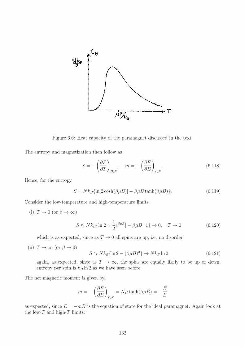
Figure 6.6: Heat capacity of the paramagnet discussed in the text.

The entropy and magnetization then follow as

S = −(∂F

∂T

)

B,N

, m = −(∂F

∂B

)

T,N

. (6.118)

Hence, for the entropy

S = NkBln[2 cosh(βµB)]− βµB tanh(βµB). (6.119)

Consider the low-temperature and high-temperature limits:

(i) T → 0 (or β → ∞)

S ≈ NkBln[2×1

2eβµB]− βµB · 1 → 0, T → 0 (6.120)

which is as expected, since as T → 0 all spins are up, i.e. no disorder!

(ii) T → ∞ (or β → 0)S ≈ NkBln 2− (βµB)2 → NkB ln 2 (6.121)

again, as expected, since as T → ∞, the spins are equally likely to be up or down,entropy per spin is kB ln 2 as we have seen before.

The net magnetic moment is given by,

m = −(∂F

∂B

)

T,N

= Nµ tanh(βµB) = −EB

as expected, since E = −mB is the equation of state for the ideal paramagnet. Again look atthe low-T and high-T limits:

132

Figure 6.7: Entropy and net magnetisation of the spin-1/2 paramagnet with non-interactingspins as a function of temperature.

(i) T → 0 (or β → ∞)m→ Nµ (6.122)

for all spins are up; and

(ii) T → ∞ (or β → 0)

m ≈ Nµ2B

kBT, Curie′s law

→ 0

again, as expected, since we have nearly equal numbers of up and down spins.

We plot S and m versus T for several different external fields as shown in Fig. 6.7.

6.9.5 The third law of thermodynamics

As we have seen above, the entropy S tends to zero as T → 0 as all spins align. This isgenerally true, namely, a system has no disorder in the limit of T → 0. This is the

Third law of thermodynamics:The entropy of any system S → 0 as T → 0.

In the next section, we discuss a way to reach low temperature limit using paramagnets.

[Refs.: (1) Mandl 3; (2) Bowley and Sanchez 5.7.]

6.9.6 Adiabatic demagnetization and the third law of thermodynamics*

By magnetizing and demagnetizing a paramagnet sample, while controlling the heat flow, wecan lower its temperature. To understand this refer to the curve of S vs. T for the idealparamagnet, see Fig. 6.7. Similar curves are shown for two different magnetic field strengthsin Fig. 6.8.

The procedure is as follows:

133

Figure 6.8: Illustration of the process of adiabatic demagnetisation..

Figure 6.9: Procedure of adiabatic demagnetisation: (a) Start, (b) Step 1, (c) Step 2.

134

• Step 0: Start with the sample in a magnetic field B1 at an already fairly low temperatureT1.

• Step 1, isothermal magnetization: Increase the field from B1 to B2 at constant T (i.e., incontact with heat bath). The entropy S hence decreases as spins align with the strongerfield (i.e., the system becomes more ordered).

• Step 2, adiabatic demagnetization: Now isolate the system from the heat bath and de-magnetize (i.e., reduce the magnetic field from B2 to B1). The system is isolated, so∆Q = 0, and if the process is quasistatic and reversible, ∆S = 0. From Fig. 6.8 we seethat the system’s temperature reduces from T1 to T2; note that from Eq. (6.119) S is afunction of B/T only, hence for constant S, if B is reduced, T must reduce by a samefactor.

• Iterate steps 1 and 2.

Fig. 6.9 illustrates what happens to the spins. In step 1, we increase the level spacing, but keepT constant; the population of the upper level falls. In step 2 we reduce the level spacing again,but as the process is now adiabatic (spins isolated) there is no change in level occupations,the temperature is lowered.

This is actually a practical way to reach quite low temperatures, to small fractions of 1 K.If we start with a large sample we could repeat the process with a small sub-sample, withrest acting as a heat bath. However at each repeat of Steps 1 and 2 we would reduce thetemperature by less and less, as the two curves come closer together as T → 0, see Fig. 6.8.Thus it is impossible to reach T = 0 in a finite number of steps in this way. This is just oneexample of the third law of thermodynamics: namely, either

(a) absolute zero is unattainable (in a finite number of steps) or, more precisely,

(b) The entropy of any aspect of any system, S → 0 as T → 0.

Note: Statement (b) implies that the ground state is non-degenerate so that all particles fallinto the same state as T → 0.

[Ref.: (1) Mandl 5.6.]

6.10 Vibrational and rotational energy of diatomic molecules

In the previous sections we considered a classical ideal gas of N particles. If these particles arediatomic molecules, in additio to the translational motion for the center-of-mass of a molecule,there are also vibrational and rotational modes. We consider these three types of motions asindependent of one another, hence write the partition function of N diatomic molecules as

ZN =1

N !(Z1)

N , Z1 = Zt1Z

v1Z

r1 (6.123)

where Zt1 is the one-body partition function of translational motion, given by Eq. (6.86)), Zv

1

is that of the vibrational motion, and Zr1 is that of the rotational motion.

We now compute Zv1 and Zr

1 quantum mechanically.

135

6.10.1 Vibrational energy contribution

The energy levels of a simple quantum harmonic oscillator of angular frequency ω are

ǫn =(n+

1

2

)hω, n = 0, 1, 2, · · · . (6.124)

Hence, the one-body partition function is the same as calculated in Eq. (6.89),

Z1 =∞∑

n=0

e−(n+1/2)hωβ =1

2 sinh(hωβ/2). (6.125)

Hence, the vibrational energy per molecule at temperature T is

Ev

N= −

(∂ lnZ1

∂β

)=

1

2 sinh(hωβ/2)· 2 cosh(hωβ/2) · (hω/2) (6.126)

orEv

N=

1

2hω coth(hωβ/2). (6.127)

We now consider the low-temperature limit and the high-temperature limit:

(i) T → 0 (β → ∞), coth(hωβ/2) → 1

Ev

N→ 1

2hω. (6.128)

This is the quantum mechanical ground state energy.

(ii) T → ∞ (β → 0), coth(hωβ/2) ≈ 2hωβ

,

Ev

N≈ 1

β= kBT. (6.129)

This is the result you would expect from a classical calculation (you should understandwhy).

Exercise:Using the results of Sec. 6.6.2 compute the average energy per particle for system of Ndistinguishable independent simple classical harmonic oscillators.

Remark:For most diatomic molecules, the high-T limit is effectively reached for T ≥ 1000 K.

6.10.2 Rotational energy contribution

In classical mechanics the energy of a rigid rotor with moment of inertia I, rotating withangular velocity ω (or angular momentum L = Iω) is ǫ = Iω2/2 = L2/2I (you shouldremember this from your first-year courses on classical dynamics, if you don’t then pleaserevise your classical mechanics).In quantum mechanics, the angular momentum is quantized as

L2 → ℓ(ℓ+ 1)h2, ℓ = 0, 1, 2, · · · (6.130)

136

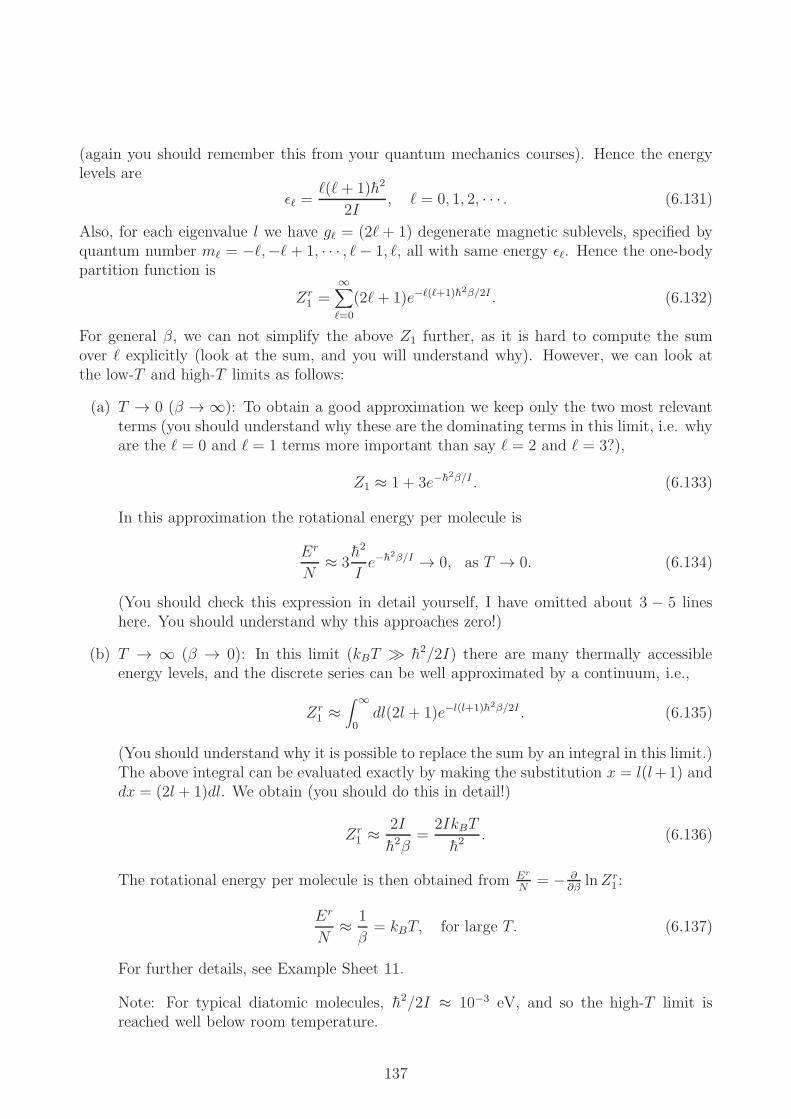
(again you should remember this from your quantum mechanics courses). Hence the energylevels are

ǫℓ =ℓ(ℓ+ 1)h2

2I, ℓ = 0, 1, 2, · · · . (6.131)

Also, for each eigenvalue l we have gℓ = (2ℓ + 1) degenerate magnetic sublevels, specified byquantum number mℓ = −ℓ,−ℓ + 1, · · · , ℓ− 1, ℓ, all with same energy ǫℓ. Hence the one-bodypartition function is

Zr1 =

∞∑

ℓ=0

(2ℓ+ 1)e−ℓ(ℓ+1)h2β/2I . (6.132)

For general β, we can not simplify the above Z1 further, as it is hard to compute the sumover ℓ explicitly (look at the sum, and you will understand why). However, we can look atthe low-T and high-T limits as follows:

(a) T → 0 (β → ∞): To obtain a good approximation we keep only the two most relevantterms (you should understand why these are the dominating terms in this limit, i.e. whyare the ℓ = 0 and ℓ = 1 terms more important than say ℓ = 2 and ℓ = 3?),

Z1 ≈ 1 + 3e−h2β/I . (6.133)

In this approximation the rotational energy per molecule is

Er

N≈ 3

h2

Ie−h2β/I → 0, as T → 0. (6.134)

(You should check this expression in detail yourself, I have omitted about 3 − 5 lineshere. You should understand why this approaches zero!)

(b) T → ∞ (β → 0): In this limit (kBT ≫ h2/2I) there are many thermally accessibleenergy levels, and the discrete series can be well approximated by a continuum, i.e.,

Zr1 ≈

∫ ∞

0dl(2l + 1)e−l(l+1)h2β/2I . (6.135)

(You should understand why it is possible to replace the sum by an integral in this limit.)The above integral can be evaluated exactly by making the substitution x = l(l+1) anddx = (2l + 1)dl. We obtain (you should do this in detail!)

Zr1 ≈ 2I

h2β=

2IkBT

h2. (6.136)

The rotational energy per molecule is then obtained from Er

N= − ∂

∂βlnZr

1 :

Er

N≈ 1

β= kBT, for large T. (6.137)

For further details, see Example Sheet 11.

Note: For typical diatomic molecules, h2/2I ≈ 10−3 eV, and so the high-T limit isreached well below room temperature.

137

6.10.3 Translational energy contribution

In Eq. (6.98) we have obtained the translational energy per molecule in an ideal gas as

Et

N=

3

2kBT. (6.138)

Remark:We have now established that, in the high-temperature limit, the energy per particle is kBTfor vibrational degrees of freedom, kBT for rotational degrees of freedom, and kBT per trans-lational degree of freedom. This is of course not an accident. These are examples of theso-called equipartition theorem, which we will discuss in Sec. 6.11.

[Refs.: (1) Bowley and Sanchez 5.11, 5.12.]

6.11 The equipartition theorem

The last three results (for vibrational, rotational and translational motion) provide examplesof the equipartiton theorem.We first state and prove the theorem in its general form for the canonical ensemble2:

Equipartition theorem:Consider a classical physical system with Hamiltonian (energy function) H = H(q1, . . . , qM),where q1, . . . , qM are generalised coordinates (degrees of freedom). Then the following holds

⟨qk∂H

∂qℓ

⟩= δkℓkBT. (6.139)

Remark 1:The average 〈f(q1, . . . , qM)〉 in the above theorem denotes the usual average in the canonicalensemble,

〈f(q1, . . . , qM)〉 = 1

Z

∫dq1 · · · dqMe−βH(q1,...,qM )f(q1, . . . , qM). (6.140)

Remark 2:The generalised coordinates (degrees of freedom), q1, . . . , qM represent the usual classical de-grees of freedom. For example, for N particles of a mono-atomic ideal gas, we have 6N totaldegrees of freedom, three spatial coordinates per particle, and three components of the parti-cle’s momentum. In this case M = 6N . The first 3N variables q1, . . . , q3N could represent thepositions of the N particls, and the remaining q3N+1, . . . , q6N coordinates their momenta.

Remark 3:I have been very sloppy with factors of h3N in the phase space measure. If Z is defined asZ =

∫ d3N rd3Nph3N e−βHN , then the corresponding definition of the phase-space average reads

〈f〉 = 1

Z

∫d3Nrd3Np

h3Ne−βHNf(r1, . . . , r3N , p1, . . . , p3N ). (6.141)

Note that for averages it does not matter whether you include the factors of h or not, as longas you are consistent. If they are included they appear in the numerator and the denominator,

2The theorem can be shown to hold in the microcanonical ensemble as well.

138

so they drop out either way. Important: When you calculate partition functions, it is crucialto include the factors of h, otherwise you get object such as Z, F etc wrong.

Proof of the theorem:The average

⟨qk

∂H∂qℓ

⟩can be written as

⟨qk∂H

∂qℓ

⟩=

1

Z

∫dq1 · · · dqM

(qk∂H

∂qℓ

)e−βH

= − 1

β

1

Z

∫dq1 · · · dqM qk

(∂

∂qℓe−βH

)(6.142)

We now integrate by parts on the right-hand-side:

⟨qk∂H

∂qℓ

⟩=

1

β

1

Z

∫dq1 · · · dqM

∂qk∂qℓ

e−βH , (6.143)

assuming that we can ignore the boundary term qke−βH , i.e. that this term vanishes at the

boundaries qk → ±∞ (this is not an unreasonable assumption).One now uses ∂qk

∂qℓ= δkℓ (Kronecker delta) and arrives at

⟨qk∂H

∂qℓ

⟩= δkℓ

1

β

1

Z

∫dq1 · · · dqM e−βH , (6.144)

Remembering that Z =∫dq1 · · ·dqM e−βH we are done,

⟨qk

∂H∂qℓ

⟩= δkℓ

1β= δkℓkBT , q.e.d.

Many physical systems have quadratic degrees of freedom (i.e. degrees of freedom that enterquadratically into the energy function, H). For such systems the equipartition theorem canbe formulated as follows:Equipartition theorem for quadratic degrees of freedom:For a physical system in which degrees of freedom contribute quadratically to the total energyfunction H the average energy is kBT/2 per degree of freedom and its contribution to the heatcapacity is kB/2. This holds for classical systems. For quantum systems the statement appliesat high enough temperatures.

Exercise (highly recommended!):Derive this statement (average energy for quadratic degrees of freedom is kBT/2 for classicalsystems) from the above general equipartition theorem. See also example sheet 11.

Examples:Here are the examples we have discussed earlier:

• Vibrations:

Evib =1

2mx2 +

1

2kx2 (6.145)

Two quadratic degrees of freedom (d.o.f.): ⇒ E ≈ kBT .

• Rotations: Two perpendicular axes about which the molecule can rotate,

Erot =1

2I1θ

21 +

1

2I2θ

22 (6.146)

Two quadratic d.o.f., hence E ≈ kBT .

139

Figure 6.10: Illustration of the specific heat as a function of temperature for a diatomic gas.

• Translations:

Etr =1

2m(x2 + y2 + z2) (6.147)

Three quadratic d.o.f., hence E ≈ 3kBT/2.

The equipartition theorem is a classical theorem. From our present statistical mechanicstreatment of quantum systems we see it breaks down when the separation between quantumenergy levels is small compared with kBT . If this happens the heat capacity of a particulard.o.f. will be reduced, dropping to zero at low temperatures. The corresponding d..o.f. is thensaid to be frozen out; e.g., this is typically the situation for the vibrational degrees of freedomat room temperature. More specifically, in quantum systems equipartition holds

• for vibrations, when T ≫ hω/kB ≈ 103 K;

• for rotations, when T ≫ h2/IkB ≈ 10− 100 K;

• for translations, when T ≫ h2/(mV 2/3kB) ≈ 10−14 K.

Thus, at room temperature, only the rotational and translational degrees of freedom can betreated classically, giving CV = 3R/2 for monatomic gases and Cv = 5R/2 for diatomic gases,for the molar heat capacity.

The diagram shown in Fig. 6.10 illustrates this for the example for a diatomic gas (e.g., H2).We can predict the heat capacities of other substances using equipartition, simply by countingthe quadratic degrees of freedom. An example is a solid, for which we expect the molarheat capacity to be 3R since each atom is free to to vibrate in 3 directions. This is theDulong-Petit law, which works well for many solids at room temperature

[Refs.: (1) Mandl 7.9; (2) Bowley and Sanchez 5.14.]

6.12 The Maxwell-Boltzmann velocity distribution

In this section we derive the Maxwell-Boltzmann velocity distribution for an ideal classicalgas you have learned in your year one module.

140

Consider a gas of N molecules in a volume V , in thermal equilibrium at a temperature T .From the Boltzmann distribution function the probability to find a particular particle in theone-particle state (r, p) is

ρ(r, p) =1

Z1

e−H1(r,p)/(kBT ) (6.148)

where H1(r, p) is the energy of the a single molecule in state (r, p). The average number ofmolecules inside a phase space volume d3rd3p/h3 centred around (r, p) is then given by

Nρ(r, p)d3rd3p

h3. (6.149)

You should at this point understand exactly why this is so. If you do not then please go backand study the sections on probability densities for continuous states (Sec. 5.3.3).We now ask how many of the N particles will have velocity v on average? Note that v =√v2x + v2y + v2z . The corresponding probability distribution P (v) is the so-called Maxwell-

Boltzmann distribution. If P (v) is the resulting probability distribution, i.e. P (v)dv is theprobability to find a given particle to have a velocity between v and v+ dv, then the expectedtotal number of particles with a velocity in this interval is NP (v)dv.

For the ideal gas we have H1(r, p) =p2

2mwith p = mv. We can therefore replace d3p by m3d3v.

Introducing the dummy variable v′ and writing d3v′ = sinϑv′2dv′dφdϑ we have

P (v) =m3

Z1

∫d3rd3v′

h3δ(v′ − v)e−βH1(r,p=mv′)

=m3

Z1

∫d3rdv′dφdϑ

h3sin ϑv′2δ(v′ − v)e−βH1(r,p=mv′)

=Vm3

Z1h3v2e−βH1(p=mv) ×

∫ 2π

0dφ∫ π

0dϑ sinϑ

=4πV m3

Z1h3v2e−βH1(p=mv)

=4πV m3

Z1h3v2e−(mv2)/(2kBT )). (6.150)

Using our earlier result for the single-particle partition function for the ideal gas (see e.g. Eq.(6.86))

Z1 = V

(mkBT

2πh2

)3/2

, (6.151)

we have

P (v) =

√2

π

(m

kBT

)3/2

v2e−mv2/(2kBT ). (6.152)

Notice the normalization (which you should check!)∫ ∞

0P (v)dv = 1. (6.153)

This is the well-known Maxwell-Boltzmann velocity (speed) distribution. We plot distributionP (v) in Fig. 6.11.A few physical quantities are calculated as follows.

141

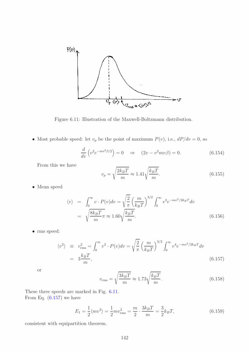
Figure 6.11: Illustration of the Maxwell-Boltzmann distribution.

• Most probable speed: let vp be the point of maximum P (v), i.e., dP/dv = 0, so

d

dv

(v2e−mv2β/2

)= 0 ⇒ (2v − v2mvβ) = 0. (6.154)

From this we have

vp =

√2kBT

m≈ 1.41

√kBT

m. (6.155)

• Mean speed

〈v〉 =∫ ∞

0v · P (v)dv =

√2

π

(m

kBT

)3/2 ∫ ∞

0v3e−mv2/2kBTdv

=

√8kBT

mπ ≈ 1.60

√kBT

m. (6.156)

• rms speed:

〈v2〉 ≡ v2rms =∫ ∞

0v2 · P (v)dv =

√2

π

(m

kBT

)3/2 ∫ ∞

0v4e−mv2/2kBTdv

= 3kBT

m, (6.157)

or

vrms =

√3kBT

m≈ 1.73

√kBT

m. (6.158)

These three speeds are marked in Fig. 6.11.From Eq. (6.157) we have

E1 =1

2〈mv2〉 = 1

2mv2rms =

m

2· 3kBT

m=

3

2kBT, (6.159)

consistent with equipartition theorem.

142

Remark:Planck’s constant (h) appears in the phase-space volume and in the partition function, butit does not feature in the Maxwell-Boltzmann distribution. Otherwise one would not be ableto deduce the Maxwell-Boltzmann distribution from classical arguments alone, e.g. from thekinetic theory of gases, as was done originally by Maxwell.

Remark:In the above calculations, we have used the following general Gaussian integral

∫ ∞

0x2ne−ax2

dx =1 · 3 · 5 · · · (2n− 1)

2n+1an

√π

a. (6.160)

[Refs.: (1) Mandl 7.7; (2) Bowley and Sanchez 7.4.]

143

Chapter 7

What’s next?*

“We can only see a short distance ahead, but we can see plenty there that needs tobe done.”

(Alan Turing)

Remark:This chapter is not examinable!

7.1 Interacting systems

So far, we have completely ignored interactions between constituent particles in all of ourexamples, from the ideal spin-1/2 paramagnets to the classical ideal gas. All partition functionsfactorized, which made our calculations rather easy.Clearly, the investigation of the effects due to, for example, interactions between molecules of agas is the next main task. In fact, the most interesting physics emerges from such interactions.Examples are phase transitions from gases to liquids or solids as temperature is lowered, andeven to superfluids or superconductors at extremely low temperatures where quantum physicsdominates.The material we have covered so far does – in principle – provide the formalism to tackle mostof these problems, although some special techniques will be required.We illustrated this using a gas of N identical classical molecules. We now explicitly acknowl-edge that these molecules interact with one another, let us assume the interaction is describedby a pair-wise interaction potential, V (r), where r is the separation between the interactingpair. We draw a typical V (r) in Fig. 7.1. Qualitatively, we see the interaction potentialconsists of a hard-core potential at small distances (molecules repel each others strongly whenthey are very close) and an attractive tail which is responsible for condensation into liquidsand formation of solids at low temperature.In Sec. 2.5.3 we have qualitatively discussed the effects due to this interaction to the equationof state, the so-called van der Waals equation,

(P +

αN2

V 2

)(V −Nβ) = NkBT, (7.1)

144

Figure 7.1: A schematic diagram for the interaction potential between two molecules.

where α and β are coefficients depending on the interaction potential. This empirical equationof van der Waals in fact provides a good description of a dense gas (recall that an ideal gascorresponds to dilute gas where interactions can be ignored) and it also predicts a phasetransition from gas to liquid phase.One of the tasks in statistical mechanics is to derive this van der Waals equation from, say,a canonical-ensemble approach. In canonical-ensemble approach, as discussed earlier, we firstneed to calculate the partition function of N molecules

ZN =∑

i

e−ǫi/kBT , (7.2)

As discussed before, the summation over microstate index i for N classical molecules corre-sponds to the integral in 6N -dimensional phase-space

∑

i

. . .→ 1

N !

1

h3N

∫d3r1d

3p1

∫d3r2d

3p2 · · ·∫d3rNd

3pN . . . . (7.3)

The factor 1/N ! is due to the property of identical particles, as described earlier. The energyǫi is then the classical Hamiltonian (total energy) of the N interacting molecules:

H = H(r1, r2, ; p1, p2, . . .) = K + U ; (7.4)

K =p212m

+p222m

+ · · ·+ p2N2m

=N∑

k=1

p2k2m

, (7.5)

U = V (|r1 − r2|) + V (|r1 − r3|) + · · · =∑

k<ℓ

V (|rℓ − rk|), (7.6)

where K is the total kinetic energy, U the total potential energy. Hence, the partition functionof the gas is written as

ZN =1

N !

1

h3N

∫d3r1d

3p1

∫d3r2d

3p2 · · ·∫d3rNd

3pNe−(K+U)/kBT .

We notice, contrast to the case of an ideal gas, the above multi-dimensional integral isnot separable (you should understand what this means!) due the coupling terms in the poten-tial U between molecular coordinates r1, r2, . . . , rN . We note that the kinetic term K is stillseparable, hence the integrals over momenta p

1, p

2, . . . , p

Ncan be factorized and computed

one-by-one separately (you should understand what this means, and how this is done!).

The problem is the interaction part in the potential energy. Special techniques have beendeveloped to evaluate this multi-dimensional integral. Broadly speaking, there are two sets oftechniques:

145

(i) Analytical methods, i.e. ‘pen-and-pencil’ calculations. For interacting systems, thesecan only be carried out in approximation, and ultimately, they result in equations whichcan only be dealt with numerically. One of such techniques is the so-called cluster-expansion for the factor e−U/kBT , or other series expansion techniques. Corrections tothe ideal gas equation of state can then be evaluated.

(ii) Monte Carlo simulations. We will discuss these in the next section.

7.2 Monte Carlo methods

Consider a system of N distinguishable spins (spin-1/2), si, i = 1, . . . , N . Say these spins arearranged on a square lattice so that each spin has four nearest neighbours.Each spin can be in one of two states, ‘up’, si = 1, or ’down’, si = −1. In an external fieldB, and setting the magnetic moment of each spin to µ = 1 for simplicity, the total energy ofsuch a system is

H = −B∑

i

si (7.7)

(you should understand why). We have here gone to a dimensionless representation, i.e. Iignore units.Rea-world spin systems have interactions between the spins. The celebrated Ising model forexample has the energy function

H(s1, . . . , sN) = −B∑

i

si − J∑

<i,j>

sisj, (7.8)

where∑

<i,j> indicates a sum of neares-neighbour pairs, (i, j). The quantity J > 0 is aninteraction coefficient. The second term in this Hamiltonian makes neighbouring spins wantto align, the energy contribution, −Jsisj of an aligned pair (si and sj have the same sign, i.e.sisj = 1) is lower than that of a pair which is not aligned (si and sj have opposite signs, i.e.sisj = −1).

This model describes ferromagnetic behaviour at low temperatures. It has a phase transitionbetween a paramagnetic phase and a ferromagnetic phase, provided we are in at least twodimensions (i.e. square lattice, cubic lattice etc). There is no phase transition in the Isingmodel in one dimension (spins situated along a one-dimensional chain).The canonical partition function of this model is

Z(β) =∑

si

e−βH(s1,...,sN), (7.9)

keep in mind that this is a function of temperature (or equivalently of β). If the function Z(β)is known explicitly all thermodynamic quantities can be derived (you should know how). Thesum in Z is over all microstates. How many of these are there (you should know the answer)?Well, each spin can be in two states (up or down), and there are N spins, so there are 2N

terms in this sum.Following issues:

• Due to the interaction we cannot do the sum analytically (pencil and paper).

146

• It is not feasible to compute this numerically either, there are just too many terms inthe sum (keep in mind that N can be very large.

Monte-Carlo methods sample a representative subset of all 2N configurations. This is knownas importance sampling. A commonly used algorithm is the so-called Metropolis algorithm,which works roughly as follows:

1. Start from a random spin configuration, i.e. assign the si = ±1 randomly.

2. In each simulation step pick one specific spin at random, say spin number i is picked.Then compute the energy difference if this spin were to be flipped (i.e. if its sign isreversed), i.e.

∆E = H(s1, . . . , si−1,−si, si+1, . . . , sN)−H(s1, . . . , si−1, si, si+1, . . . , sN). (7.10)

If ∆E < 0 flip the spin, and goto 2, i.e. pick a new spin for potential flip, and repeat.

If ∆E > 0 flip the spin with probability

p = e−β∆E (7.11)

(and with probability 1− p do not flip it). Then goto 2, i.e. pick a new spin and repeat.

This algorithm will produce a sequence of spin-configuations, and one can show that av-eraging over the spin configurations so obtained approximates the canonical average (overthe 2N terms in the partition function) very well. If the sequence of spin configurations iss(1), s(2), . . . , s(tfinal), then for example

〈E〉 ≈ 1

tfinal

tfinal∑

t=1

H(s). (7.12)

Good results are obtained without having to generate all 2N possible configurations s =(s1, . . . , sN). The ‘importance sampling’ of the algorithm makes sure that only the mostrelevant configurations are sampled.

There is a second-year Theory Computing Project which uses this technique to investigatethe phase transition of the Ising model. Similar techniques are used in a variety of physicsproblems, including in particle physics, e.g. Monte-Carlo simulations of lattice gauge fieldtheories (for example lattice QCD).

The Monte-Carlo method defines a stochastic process in the space of configurations. Thisinvolves stochastic dynamics (i.e. ‘hopping’ from one microstate to the next).

Some of these models with an actual dynamics are discussed in the fourth year module onAdvanced Statistical Physics. See also the section on non-equilibrium systems below, Sec. 7.5.

7.3 Systems with variable particle numbers

So far, we have mostly looked at systems with a constant number of particles. In the micro-canonical ensemble both energy and particle numbers are fixed. In the canonical ensembleenergy can fluctuate (hence the Boltzmann factor, e−βE), but particle numbers are fixed.

147

The so-called grand canonical ensemble describes systems which can exchange of particles withthe environment. A microstate i of the system is the characterised by its energy, Ei, and bythe particle number, Ni in that microstate. The notion of the canonical partition function isextended to give the

Grand-canonical partition function:

Z(µ, T, V ) =∑

i

e−β(Ei−µNi), (7.13)

where µ is the chemical potential.

The corresponding statistics are given by the

Grand-canonical ensemble:

pi =1

Z e−β(Ei−µNi), (7.14)

pi is the probability to find the system in microstate u, with energy Ei and particle numberNi.The corresponding bridge equation is

ΦG = 〈E〉 − TS − µ 〈N〉 = − 1

βlnZ, (7.15)

where ΦG is the so-called grand potential.

The grand canonical ensemble is crucial for the discussion of quantum gases. It will be coveredin detail in the third-year module on Bose and Fermi gases.

7.4 Quantum systems

Most of the calculations in this course were classical calculations. Some of the few actualquantum calculations were carried out only in the large-temperature limit, where they effec-tively become classical. We have neglected the properties for example of Bosons occupying thesame single-particle state (particularly the quantum ground m state) when we discussed theindependent-particle approximation for identical particles. Such effects are important in thelow temperature limit and inclusion of such quantum effects will result in the Bose-Einsteincondensation. Electrons in conductors and other solid state systems are Fermions, and theirstatistical mechanics requires a full quantum approach.The classical formalism we have covered is however somewhat analogous to the quantum case.For example, the classical Hamiltonian, H(r, p), is to be replaced by the quantum mechanical

Hamilton operator, H, and the Gibbs entropy

S = −kB∑

i

pi ln pi, (7.16)

is replaced by the von-Neumann entropy

S = −kBtr ρ ln ρ , (7.17)

148

where ρ is the density operator describing the system at hand. This is formally an infinite-dimensional matrix, tr describes its trace (sum of the diagonal elements). The quantummechanical ensembles (microcanonical, canonical, grand canonical) can then be obtained bymaximising the von Neumann entropy (7.17) subject to the appropriate constraints. This isagain done using Lagrange multipliers.

These issues will be discussed in more detail in the third-year course on Bose and Fermi gases.

7.5 Non-equilibrium dynamics

All of what we have discussed is part of what is called equilibrium statistical mechanics. Noneof our calculations actually involve a dynamics. Instead what we do is to look at the distribu-tions generated by energy functions (Hamiltonian), e.g. the canonical ensemble. Compare thisto your first-year dynamics, where you study the trajectories of particles, i.e. their actual timebehaviour, say x(t), derived from differential equations (Newton). These equations explicitlyinclude time derivatives, which did not play any role in this course.

The starting point of all our calculations in the statistical physics part was the HamiltonianHN(r,p). But the mere existence of such an energy function is a severely limiting assumptions.For many systems in real life there is no energy function (or free energy), which is subject tosome minimisation principle. Instead many real-world problems are defined dynamically, by arule which characterises the time-behaviour of the system, say how to hop from one microstateto another. It is often not clear how to write down H from such rules, and more often thannot, there is no Hamiltonian.

This is relevant in almost all transport problems where the system is driven, in many biologicalapplications (life is mostly a non-equilibrium phenomenon).

The fourth year course on Advanced Statistical Physics focuses on non-equilibrium dynamics.It develops the mathematical formalism with which to characterise such off-equilibrium sys-tems. As a taster I mention the so-called ‘master equation’. Suppose the model is defined byrates (probabilities per unit time) to hop from one microstate to the next, Ti→j . So Ti→j isthe rate with which the system hops to state j if it is initially in state i.

The probability, Pi(t) to find the system in state i at time t then obeys the following differentialequation, the so-called master-equation

∂tPi(t) =∑

j 6=i

Tj→iPj(t)

︸ ︷︷ ︸inflow

−∑

j 6=i

Ti→jPi(t)

︸ ︷︷ ︸outflow

. (7.18)

Other techniques used to study such stochastic processes include stochastic differential equa-tions, the Fokker-Planck equation (a Schrodinger equation in imaginary time), path integralsetc. Some of these will be discussed in the Advanced Statistical Physics module in 4th year.

149

7.6 Interdisciplinary applications of statistical physics:

complex systems

The field of statistical physics of complex systems is a growing area of modern physics. Itdescribes the application of tools from statistical physics to questions in adjacent disciplines,for example in biology, economics and the social sciences.

Many of the models in these disciplines effectively describe interacting individuals, subject tostochastic dynamical rules. The term individual can here refer to different things, dependingon the specific application. In a model of traffic flow an individual may be an individual vehiclewhich moves forward along a road subject to certain rules. In a model of a stock market aninvididual may be a trader, who in a most basic approach can be in one of two states (buyand sell). In biology an individual may represent an individual prey or predator in a modelof population dynamics, or maybe a protein or a gene in evolutionary dynamics.

We study these topics in the Statististical Physics and Complex Systems group, see here forour web page:

http://theory.physics.manchester.ac.uk/~cssp/

Research questions we study include:

• The development of analytical techniques to study individual-based systems with stochas-tic interactions. We use tools and ideas from statistical physics to characterise suchsystems mathematically. This includes e.g. the theory of stochastic processes, stochas-tic differential equations, master equations, Fokker-Planck dynamics, path integrals andgenerating functionals, semi-classical WKB approaches, etc.

• The development of fast simulation algorithms for stochastic interacting agent models,e.g. kinetic Monte Carlo methods, the celebrated Gillespie algorithm, modified next-reaction schemes, Poissonian processes, etc.

• The application of these methods to specific problems, e.g.

– evolutionary game theory

– speciation dynamics in ecology

– the spread of epidemics in populations

– the dynamics of cancer initiation

– models of opinion dynamics and voting

– models of language evolution

– chaotic dynamics in game learning and economics

– pattern formation in stochastic systems

– ...

Relevant third and fourth year modules include

1. PHYS 30471 (Introduction to nonlinear physics): mostly about the deterministic dynamicsof complex systems.

150

2. PHYS 40571 (Advanced Statistical Physics, taught by myself from 2014): non-equilibriumstatistical mechanics, stochastic dynamics of complex systems.

3. MPhys projects in this area in semester 7 and semester 8.

If you are interested in any of these topics, come to talk to us.

151