1

Phys 2310 Mon. Sept. 12, 2015 Today’s Topics

•  Continue Chapter 33: Geometric Optics •  Reading for Next Time

TexPoint fonts used in EMF. Read the TexPoint manual before you delete this box.: AAAAAAA

2

Chapter 5: Thin Lens Combinations •  For lens combinations the object for the second lens is just the image

formed by the first. –  Be careful about the sign of the object distance (see table 5.2)

•  If d > s’1 then “object for the second lens is real. If d < s’1 then object is virtual. –  See pgs. 167-169 in Hecht for equations and also the next slide.

•  For the graphical method –  You can solve lenses graphically by laying them out in a drawing program

(or even graph paper!) and tracing the Paraxial and Chief rays –  Note that the “extra” ray (#9/10) goes through center of second lens. –  In addition, ray #6/7 is deviated by second lens and must go through F’2 so

together they (#6/7 & # 9/10) locates the new image.

3

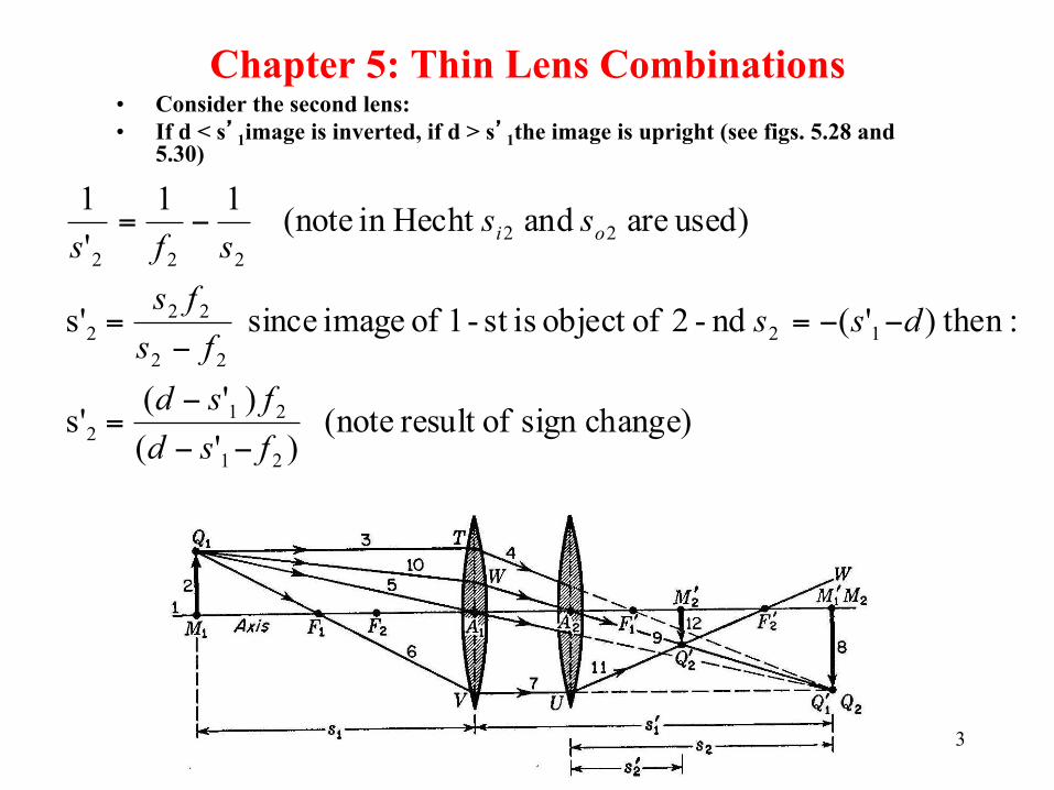
Chapter 5: Thin Lens Combinations •  Consider the second lens: •  If d < s’1image is inverted, if d > s’1the image is upright (see figs. 5.28 and

5.30)

change)sign ofresult (note )'(

)'(s'

: then)'( nd-2 ofobject isst -1 of image since s'

used) are and Hecht in (note 11'1

21

212

1222

222

22222

fsdfsd

dssfsfs

sssfs oi

−−

−=

−−=−

=

−=

4

Chapter 33: Thin Len Combinations - II

•  If the second lens is inside the focus of the first: – Convex lens

shortens the focal length (power is higher)

– Concave lens lengthens the focal length (power is negative)

5

Chapter 33: Thin Len Combinations - III •  Gaussian lens equation

can be applied to a sequence of lenses: just let the image of the first lens be the object of the second and so on. –  Be Careful with Signs!

)()( b.f.l.

)()( f.f.l.

:becomen then combinatio for the lengths focal twoThe)/()/(

:for ngsubstituti and )(

)(

:for ngsubstitutiupon and

or, 111:so and

#2) lens beyond is image theif negative becan this(Note :lens second for the Now

or, 111:LensFirst For the

21

12

21

21

11112

1111222

121

212

222

222

222

12

11

111

111

ffdfdf

ffdfdf

fsfsfdfsfsfdfs

sfsdfsds

sfsfss

sfs

sds

fsfss

sfs

oo

ooi

ii

ii

oo

oi

oi

io

o

oi

oi

+−

−=

+−

−=

−−−

−−=

−−

−=

−=

−=

−=

−=

−=

6

Chapter 33: Thin Lens in Contact

•  For lens in contact (separation is negligible) –  Object distance of lens #2 = Image distance of lens

#1 •  For an object at infinity:

power)each of sum is(power

111

:or 111

21

21

21

PPPfff

fff

+=

+=

=+−

7

Chapter 33: Image Properties - I

Sign Conventions (very important, memorize!)

8

Chapter 33: Image Properties

Convex vs. Concave Lenses

9

Chapter 33: Aperture Stops •  Note that all lenses have finite diameters (aperture stop)

–  Limits amount of light going through lens •  It can larger or smaller than the lens aperture (see fig. 5.34, 5.35)

•  Image plane also is finite (i.e., the detector): field stop –  Limits size of image

•  Internal stops in complex lens systems can help control the abberations of the lens Can also reduce illumination of the image plane as the off-axis angle increases (vignetting) –  Useful for controlling stray light in infrared instruments

•  We define the f#, or speed of a lens as f# = f/D –  The smaller the number the brighter the image (and vice versa) –  The smaller the f# the smaller the depth, or tolerance of focus

10

Chapter 33: Mirrors - I

•  Flat of Plane mirrors: – All images are virtual – Angle of reflection = angle of incidence – Object distance = image distance (fig. 5.40) – Virtual images of mirrors are reversed but

not inverted –  Images from lenses are inverted but not

reversed – Used in laser scanners, some digital

projectors, and other instances where “beam steering” is needed

Chapter 33: Plane or Flat Mirrors

•  Images with Plane Mirrors –  Location of Virtual Image

Found by tracing rays from object.

–  You see only those rays that enter your eye.

11

12

Chapter 33: Mirrors - II •  Spherical Mirrors:

–  Images can also be formed by curved mirrors

–  Concave mirrors form real images (f > 0)

–  Convex mirrors form virtual images (f < 0)

•  Focal length = 2 x Radius of Curvature

•  Aspherical Mirrors: •  From analytic geometry its clear the best axial image will be from a parabola not a sphere.

• Parabolic mirror is shape equal distance from incoming wavefront and a focus.

• However, off-axis images deteriorate rapidly.

Rss io

211−=+

13

Chapter 33: Sign Conventions

14

Example Problems

•  Consider a bi-convex lens with R1 = R2 = 15cm. a)  Determine the focal length of the lens b)  Find the image distance for an object located 35cm from the

lens c)  Make a ray diagram sketch for this configuration d)  Make a sketch of the image distance vs. object distance

15

Example Problems

•  Consider a concave spherical mirror with fl = 60cm. a)  Is the image real or virtual? b)  Find the image of an object located 10.0 m away from the

mirror c)  Make a ray diagram sketch for this configuration

•  Repeat this example for a convex spherical mirror with fl = - 60cm

16

Reading this Week By Wednesday:

Finish Ch. 33 Lenses and Prisms Begin Ch. 34 Optical Systems