.

Phylogenetic Trees:UPGMA and NN Chains

Lecture 11

Section 7.4, in Durbin et al., 6.5 in Setubal et al.© Shlomo Moran, Ilan Gronau

2

Maximum Parsimony

. Last week we presented Fitch algorithm for the “small”Maximum Parsimony problem:

Input: A rooted binary tree with characters at the leavesOutput: Assignment of characters to internal vertices which minimizes the number of mutations.

Some mutations may be more probable than others. Hence, a natural generalization of the Maximum Parsimony problem is the Weighted Parsimony, which you’ll do in the tutorial.

7

1st problem with the Maximum Parsimony Approach: Inconsistency

Maximum Parsimony may be not consistent, i.e:

In some probabilistic models of evolution of DNA (or protein) sequences, there are some scenarios of evolution, in which the most parsimonious tree is w.h.p. different from the true tree. We illustrate this on quartets: trees on four taxa. Such a tree has 3 possible topologies:

1

2

3

4

1

3

2

4

1

4

2

3

8

A quartet which is unlikely to be reconstructed by maximum parsimony

A

A A

1 4

32

Consider a model with 4 letters (DNA), where the probability for a substitution is proportional to edge length, and consider the tree below.

In this tree, characters in 2 and 3 are w.h.p. as the origin, and in 1 and 4 are more likely to be different.

9

A

A A

1 4

32

Parsimony may be useless/misleading for reconstructing the true tree

Assume the (likely) scenario where leaves 2 and 3 are the same. There are 4 patterns of substitution for leaves 1,4.

A I AA II GC III GG IV G

10

Case I all topologies get same parsimony score

A

A A

1 4

32

AA

1

2

3

4

A

A

A

A

1

3

2

4

A

A

A

A

1

4

2

3

A

A

A

A

Score=0 Score=0 Score=0

11

Case II all topologies get same score

A

A A

1 4

32

GA

1

2

3

4

A

A

A

G

1

3

2

4

A

A

A

G

1

4

2

3

A

G

A

A

Score=1 Score=1 Score=1

12

Case III …same

A

A A

1 4

32

GC

1

2

3

4

A

A

C

G

1

3

2

4

A

A

C

G

1

4

2

3

A

G

C

A

Score=2 Score=2 Score=2

13

Case III most parsimonious topology is wrong

A

A A

1 4

32

CC

1

2

3

4

A

A

C

C

1

3

2

4

A

A

C

C

1

4

2

3

A

C

C

A

Score=2 Score=2 Score=1

14

Parsimony is correct only in the least likely cases

A

C A

1 4

32

AC

For most parsimonious tree to be the correct tree, it is necessary that 2 and 3 will have different characters – which is less likely than all other cases

18

2nd problem with Maximum Parsimony (and other Character Based Algorithms):

Efficiency

There are no efficient algorithms for solving the “big”problem for maximum parsimony/Perfect phylogeny (both are known to be NP hard).

Mainly for this reason, the most used approaches for solving the big problem are distance based methods.

19

Distance-based Methodsfor Constructing Phylogenies

This approach attempts to overcome the two weaknesses of maximum parsimony:

1. It start by estimating inter-taxa distances from a well defined statistical model of evolution (distances correspond to probability of changes)

2. It provides efficient algorithms for the big problem. Basic idea: The differences between species (usually

represented by sequences of characters) are transformed to numerical distances, and a tree realizing these distances is constructed.

20

Distance-Based Reconstruction

• Compute distances between all taxon-pairs• Find a tree (edge-weighted) best-describing the distances

⎟⎟⎟⎟⎟⎟⎟⎟

⎠

⎞

⎜⎜⎜⎜⎜⎜⎜⎜

⎝

⎛

=

030980

15141801716202201615192190

D

4 5

7 21

210 6 1

22

Data Distances Trees

1. Modeling question: given the data (eg DNA sequences of the taxa), how do we define distances between taxa?

2. Algorithmic question: Decide if the distances define a tree (ultrametric or additive – to be defined later), and if so, construct that tree.

3. In reality, the computed distances are noisy. So we need the algorithm to return a tree which approximates the distances of the input data.

In the following we shall study items 2 and 1, and briefly discuss item 3.

23

Ultrametric and Tree MetricA distance metric on a set M of L objects is a function

(represented by a symmetric matrix) satisfying:d(i,i)=0, and for i≠j, d(i,j)>0d(i,j)=d(j,i).For all i,j,k it holds that d(i,k) ≤ d(i,j)+d(j,k).

A metric is ultrametric if it corresponds to distances between leaves of a tree which admits molecular clock.It is a tree metric, or additive, if it corresponds to distances between nodes in a weighted tree.

:d M M R+× →

24

1st model: Molecular Clock Ultrametric Trees

molecular clock assumes a constant rate of evolution. Namely, the distances from any extinct taxon (internal vertex) to all its current descendants are proportional to time, hence are identical.A directed tree satisfying this property is called ultrametric.

25

Ultrametric trees Definition: An ultrametric tree is a rooted weighted tree all of whose leaves are at the same depth. Basic property: Define the height of the leaves to be 0. Then edge weights can be represented by the heights of internal vertices.

A E D CB

8

5

0:3333

2

5

5

3Edge weights:

Internal-vertices heights: 3 3

26

Least Common Ancestor and distances in Ultrametric Tree

Let LCA(i,j) denote the least common ancestor of leaves i and j. Let height(LCA(i, j)) be its distance from the leaves, and dist(i,j) be the distance from i to j.

Observation: For any pair of leaves i, j in an ultrametric tree:height(LCA(i,j)) = 0.5 dist(i,j).

0E

50D

880C

8830B

35880AEDCBA

A E D CB

8

53 3

27

Ultrametric MatricesDefinition: A distances matrix* U of dimension L×L is ultrametric

iff for each 3 indices i, j, k :U(i,j) ≤ max {U(i,k),U(j,k)}.

9j69ikj

Theorem: The following conditions are equivalent for an L×L distance matrix U:

1. U is an ultrametric matrix.2. There is an ultrametric tree with L leaves

such that for each pair of leaves i,j:U(i,j) = height(LCA(i,j)) = ½ dist(i,j).

* Recall: distance matrix is a symmetric matrix with positive non-diagonal entries,0 diagonal entries, which satisfies the triangle inequality.

28

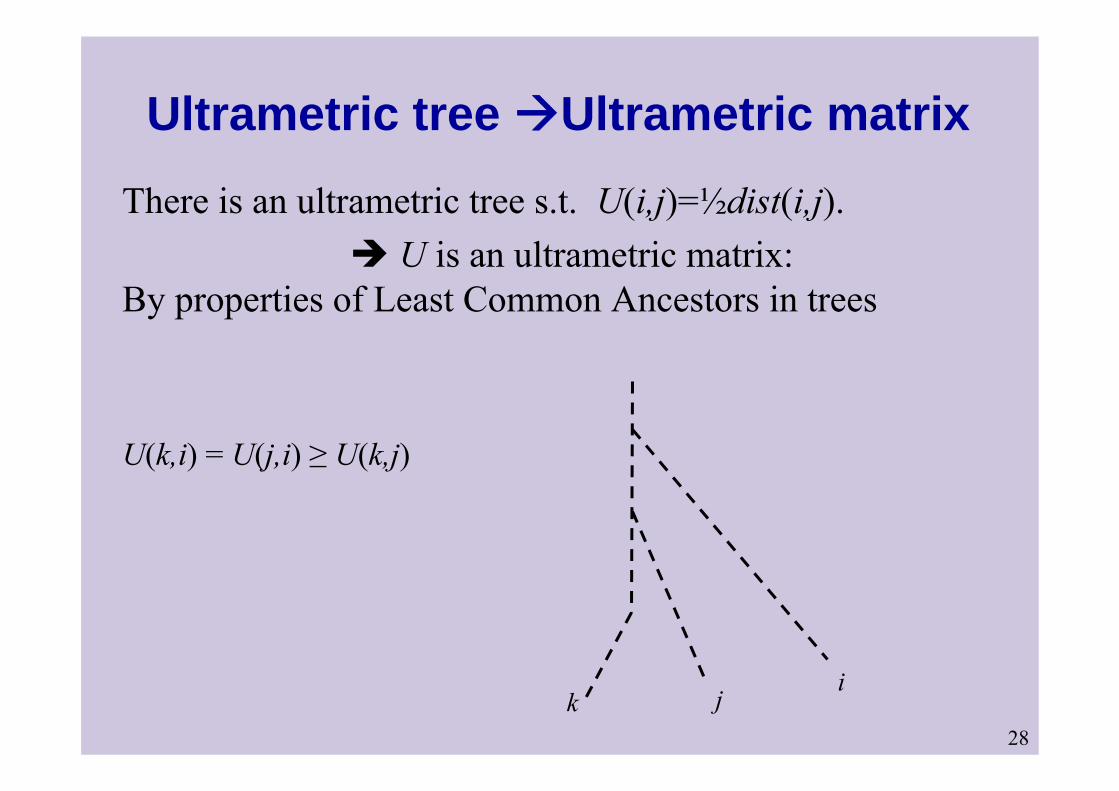
Ultrametric tree Ultrametric matrixThere is an ultrametric tree s.t. U(i,j)=½dist(i,j).

U is an ultrametric matrix: By properties of Least Common Ancestors in trees

ijk

U(k,i) = U(j,i) ≥ U(k,j)

29

Ultrametric matrix Ultrametric tree:The proof is based on the below two observations:

Definition: Let U be an L×L matrix, and let S ⊆ {1,...,L}.

U[S] is the submatrix of U consisting of the rows and columns with indices from S.

Observation 1: U is ultrametric iff for every S ⊆ {1,...,L}, U[S] is ultrametric.

Observation 2: If U is ultrametric and maxi,jU(i,j)=M, , then M appears in every row of U.

Mj

??ikj

One of the “?” Must be M

30

Ultrametric matrix Ultrametric tree:Proof by induction

U is an ultrametric matrix U has an ultrametric tree : By induction on L, the size of U.

Basis: L= 1: T is a leaf

L= 2: T is a tree with two leaves

0

90

0

i

j

i j

i

i i•

9

ji

31

Induction stepInduction step: L>2.Use the 1st row to split the set {1,…,L} to two subsets:S1 ={i: U(1,i) =M}, S2={1,..,L}-S

(note: 0<|Si|<L)

58280154321

S1={2,4}, S2={1,3,5}

32

Induction stepBy Observation 1, U1= U[S1] and U2= U[S2] are ultrametric.Let M1 (M2) be the maximal entries in U1 (U2 resp.).Note that M1≤ M, and M2 < M (M2 is the 2nd largest element in row 1( if

M2=0 then T2 is a leaf).By induction there are ultrametric trees T1 and T2 for T1 and T2.Join T1 and T2 to T with a root as shown.

T2T1

M2

M

M1

33

Proof (end)

Need to prove: T is an ultrametric tree for Uie, U(i,j) is the label of the LCA of i and j in T.If i and j are in the same subtree, this holds by induction.Else LCA(i,j) = M (since they are in different subtrees).Also, [U(1,i)= M and U(1,j) ≠ M] ⇒ U(i,j) = M.

Mi

lMji

T2T1

M2

M

M1

ij

34

Efficient Algorithms for Constructing Ultrametric Trees

Input: A distance matrix over a set S.Output: an ultrametric tree on the objects in S.(Note: we want our algorithm to be defined for all input metrics).

Requirements:Consistency: If the input matrix is ultrametric, then the

algorithm should return the corresponding tree (there is only one).

Robustness: if the input matrix is not ultrametric, the algorithm should return an ultrametric “close” to it.In this course we’ll concentrate on the 1st requirement.

35

Reconstructing Ultrametrics:UPGMA Clustering

Unweighted Pair Group Method using Averages

Input: distance matrix over a set of species S.Output: an ultrametric phylogenetic tree on S.Outline:

Initialization: Each object is a cluster. Place all clusters at height zero.At each iteration combine two “closest” clusters to get a new one, update distances to the new cluster and continue.

This clustering algorithm is used in many other applications, such as data mining.

36

UPGMAWhile(#clusters > 1) do:

• Choose cluster pair i,j as neighbors, s.t.D(i,j) = mini’≠j’{ D(i’,j’) }

• Connect i,j to new cluster v• Replace in D the pair i,j by v, and reduce D:

For k≠v, D(v,k) = αD(i,k) + (1-α)D(j,k)||||

||

ji

i

CCC+

=α

By induction on the # of iterations, this reduction formula guarantees that the distance between clusters Ci and Cj is the average of distances between the elements in each cluster:

1( , ) ( , )| || |

i j

i jp C q Ci j

d C C d p qC C ∈ ∈

= ∑ ∑

38

Reduction Formulas in “Closest Pair” Clustering Algorithms

The reduction formula (computing distances from new clusters) ofUPGMA has several variants, for instance:

For k≠v, D(v,k) = ½( D(i,k) + D(j,k) ) WPGMAor D(v,k) = min{D(i,k),D(j,k)} Single linkage

Both these reduction keep the consistency of the algorithm.It is known (by simulations) that the chosen reduction formula may have a significant effect on the robustness of the algorithms to noise.

40

Consistency of UPGMA

Proposition: If the input distances are ultrametric, then UPGMA will reconstruct the corresponding ultrametrictree T.

Proof sketch: By induction on the number of iterations, show that the distance between two clusters is twice the height of the LCA of the corresponding subtrees.

Ci CjCv

41

Complexity of UPGMA

•Naïve implementation: n iterations, O(n2) time for each iteration (to find a closest pair) O(n3) total.•Constructing heaps for each row and updating them each iteration O(n2log n) total• Optimal implementation: O(n2) total time. One such implementation, using “mutually nearest neighbors” is presented next.

42

The “Nearest Neighbor” Algorithm Let D be a distance metric.j is a nearest neighbor (NN) of i if

[ ] & [ ( , ) min{ ( , ) : }]j i d i j d i k k i≠ = ≠

( , ) min{ ( , ), ( , ) : , }d i j d i k d j k k i j≤ ≠

(i, j) are mutual nearest neighbors if:i is NN of j and j is NN of i .

In other words, if:

43

Ultrametric Reconstruction by Nearest Neighbor Chains algorithm

n-1 neighbor-joining iterations

While(#clusters > 1) do:

• Choose cluster pair i,j which are mutual nearest neighbors• Connect i,j to new cluster v• Replace i,j with the cluster v, and reduce the distance matrice D:

For k≠v, D(v,k) = αD(i,k) + (1-α)D(j,k)

| | in UPGMA, but the algorithm is consistent for any 0 1.| | | |

(i.e., if the reduction is )

i

i j

CC C

convex

α α= ≤ ≤+

44

00

00

00

00

00

0

Finding mutual nearest neighbors in O(n2) total time:

Mutual NN

i0

i1

i0 i1

i1

i2

i2

Complete NN chain:• ir+1 is a Nearest Neighbour of ir

• Final pair (il-1 ,il ) are mutual nearest neighbors.

D:

θ(n2) implementation of NN chains

3 6 4 5 8 2 6 9 3 2

5 7 3 2 4 8 1 9 7 6

2 1

• Find minimal entry (ir ,ir+1) in row ir. ir+1 is a nearest neighbour of ir.

• Stop if (ir ,ir+1) is also minimal in row ir+1

(i.e., (ir ,ir+1) are mutual nearest neighbours)

• Otherwise, continue.

45

An θ(n2) implementation using Nearest Neighbors Chains:

- Extend a chain until it is complete.

- Select final pair (i,j) for joining. remove i,j from chain, join them to a

new vertex v, and compute the distances from v to all other vertices.

Note: in the reduced matrix, the remaining chain is still NN chain, i.e. ir+1 is still the

nearest neighbor of ir - since v didn’t become a nearest neighbor of any vertex in the NN chain (since i and j were not)

Mutual NN

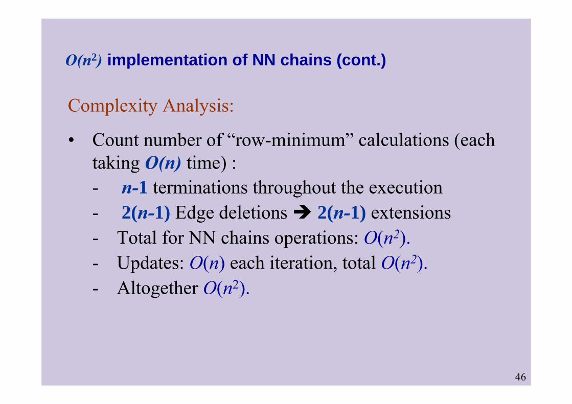
θ(n2) implementation of NN chains (cont.)

i j

46

Complexity Analysis:

• Count number of “row-minimum” calculations (each taking O(n) time) :- n-1 terminations throughout the execution- 2(n-1) Edge deletions 2(n-1) extensions - Total for NN chains operations: O(n2).- Updates: O(n) each iteration, total O(n2).- Altogether O(n2).

O(n2) implementation of NN chains (cont.)