1

PHY 042: Electricity and Magnetism

Electrodynamics

Prof. Hugo Beauchemin

2

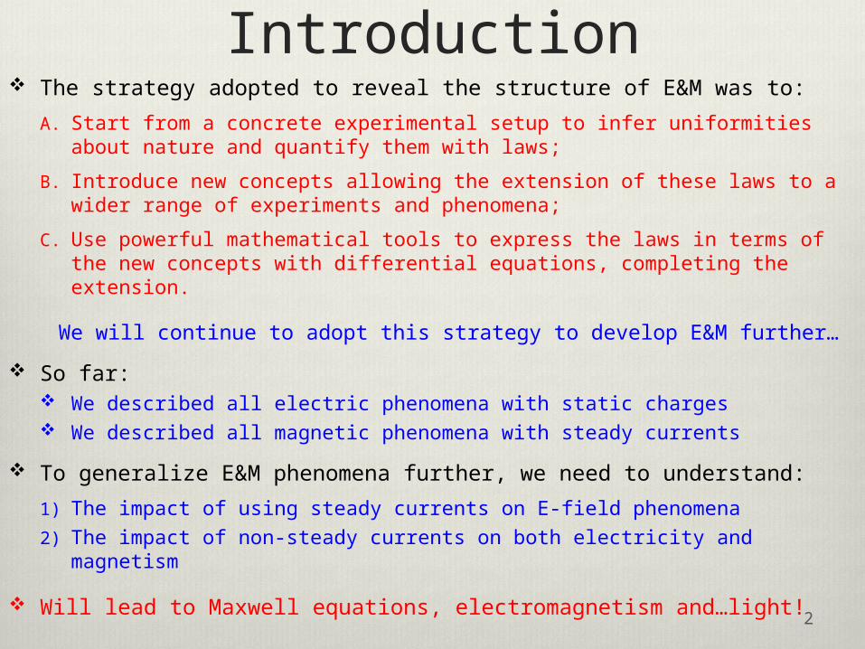
Introduction The strategy adopted to reveal the structure of E&M was to:

A. Start from a concrete experimental setup to infer uniformities about nature and quantify them with laws;

B. Introduce new concepts allowing the extension of these laws to a wider range of experiments and phenomena;

C. Use powerful mathematical tools to express the laws in terms of the new concepts with differential equations, completing the extension.

We will continue to adopt this strategy to develop E&M further…

So far: We described all electric phenomena with static charges We described all magnetic phenomena with steady currents

To generalize E&M phenomena further, we need to understand:

1) The impact of using steady currents on E-field phenomena

2) The impact of non-steady currents on both electricity and magnetism

Will lead to Maxwell equations, electromagnetism and…light!

Ohm’s law The connection between electric fields and steady currents

begin again with an experimental setup:

A device to set charges in motion, i.e. to generate an E-field:

Voltaic pile generates a potential difference

A source of free charges that can move in the E-field:

Metallic wire allows for steady currents

Ohm measured the relationship between current (moving charges) and potential (electric field) and found an empirical law:

R depends on the nature of the material and its geometry Uses newly made galvanometer to measure currents when varying

V

We want a connection between a steady current and the E-field:3

Charges move in response to an E-field

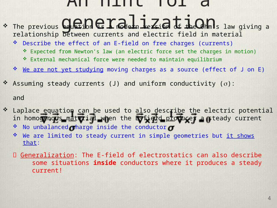
An hint for a generalization The previous equation is a modern version of the Ohm’s law giving

a relationship between currents and electric field in material Describe the effect of an E-field on free charges (currents)

Expected from Newton’s law (an electric force set the charges in motion) External mechanical force were needed to maintain equilibrium

We are not yet studying moving charges as a source (effect of J on E)

Assuming steady currents (J) and uniform conductivity (s):

and

Laplace equation can be used to also describe the electric potential in homogenous material when the E-field produces a steady current No unbalanced charge inside the conductor We are limited to steady current in simple geometries but it shows

that:

Generalization: The E-field of electrostatics can also describe some situations inside conductors where it produces a steady current! 4

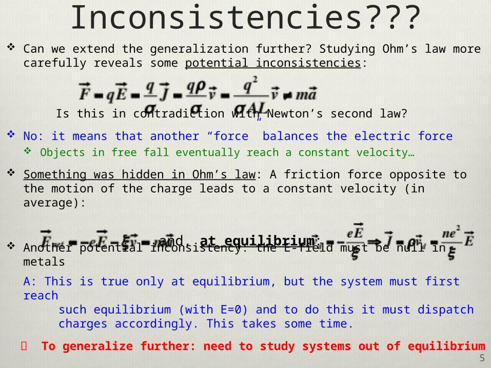
Inconsistencies??? Can we extend the generalization further? Studying Ohm’s law

more carefully reveals some potential inconsistencies:

Is this in contradiction with Newton’s second law?

No: it means that another “force” balances the electric force Objects in free fall eventually reach a constant velocity…

Something was hidden in Ohm’s law: A friction force opposite to the motion of the charge leads to a constant velocity (in average):

Another potential inconsistency: the E-field must be null in metals

A: This is true only at equilibrium, but the system must first reach such equilibrium (with E=0) and to do this it must dispatch charges accordingly. This takes some time.

To generalize further: need to study systems out of equilibrium 5

and, at equilibrium:

6

Ensuring equilibrium Ohm’s law implies that a friction insures constant velocity for

the charge carrier, but doesn’t stop the motion there is something else

Q1: How is it possible that the current is the same in each segment of a circuit, i.e. that the current is constant (I=V/R)?

Q2: Why currents circulate so quickly in a circuit while the drift velocity of charge carrier is small

A1: The E-field distributes charges in the conductor in such a way to reach equilibrium and this guarantees steady current

If current varies, it means that for a given segment Iin≠Iout

Charge will accumulate, generating an E-field removing the charge accumulation and restoring Iin=Iout. The current is steady, in average

A2: Intermediate charges relay the effect of E to each others at the speed of light, but charge reaction might be slow in average

But there is more…★ From Q1 and Q2: we discussed how an E-field, the same as the

one described in electrostatics, propagates in the circuit, moves charges around and reach an equilibrium state in the most efficient way

This describes the situation in the wires, but this is not the full circuit What is the origin of this E-field satisfying electrostatic field equations? Why doesn’t the friction kill the current?

There is another electric force, beside the electrostatics field in the wire, which is involved in a Ohm’s circuit:

The force of the source of potential fs, contained in the battery Doesn’t need to be a battery (chemical reaction) to provide the source of

energy, could be piezoelectric, thermocouple, etc.

To make sense of the empirical Ohm’s law, there must be:1. a dissipative force;

2. a source force, confined to a small part of the circuit, doing work on the system to compensate dissipation;

3. E-force of electrostatics propagating the effect of the source elsewhere7

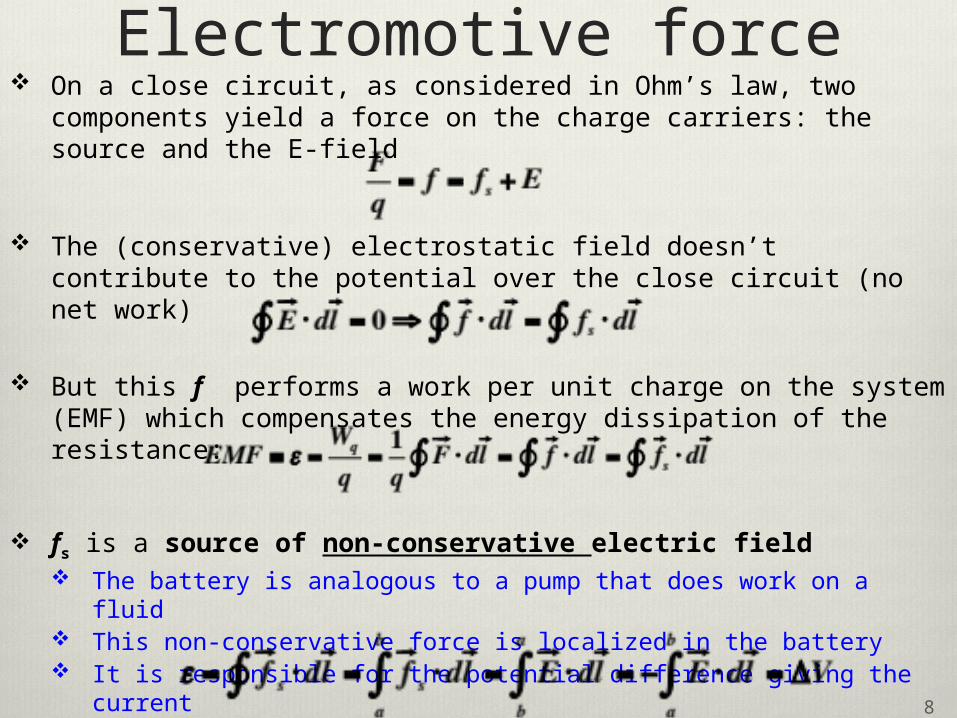
Electromotive force On a close circuit, as considered in Ohm’s law, two

components yield a force on the charge carriers: the source and the E-field

The (conservative) electrostatic field doesn’t contribute to the potential over the close circuit (no net work)

But this f performs a work per unit charge on the system (EMF) which compensates the energy dissipation of the resistance:

fs is a source of non-conservative electric field The battery is analogous to a pump that does work on a fluid This non-conservative force is localized in the battery It is responsible for the potential difference giving the current

8

9

Motional EMF (I) Studying EMF is the best prospect for a complete

generalization of electrostatics: it is a non-conservative field

An EMF converts some form of energy into an electric potential

Let’s consider devices that convert mechanical works into electric potential using… a magnetic field: generators

Pull the conducting bar at speed v

Free charge in the bar are subject to a magnetic force along the bar

Moving charges = current EMF

The EMF is localized in the bar

Motional EMF (II) Q1: How could the magnetic force generate an EMF if it does no work on a system (normal to the direction of motion)

Q2: How could the magnetic field keep the current for more than an infinitesimal fraction of the time after the start of motion?

F is always normal to the direction of motion

The expression of the EMF in terms of B is partly misleading:

the work converted by the EMF to potential, doesn’t come from the constant magnetic field, but from the force pulling the circuit

The magnetic field is transmitting the force to produce the current The magnetic force generate a resistance that must be balanced by

the external force to keep the current constant

10✔

11

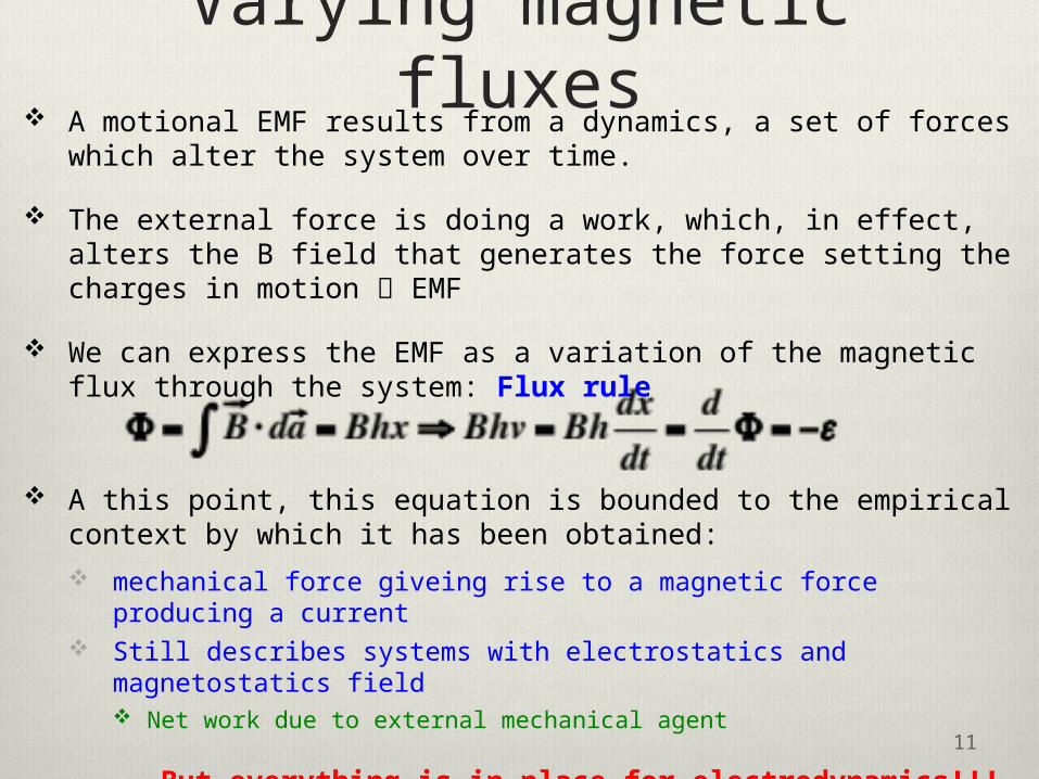
Varying magnetic fluxes A motional EMF results from a dynamics, a set of forces which

alter the system over time.

The external force is doing a work, which, in effect, alters the B field that generates the force setting the charges in motion EMF

We can express the EMF as a variation of the magnetic flux through the system: Flux rule

A this point, this equation is bounded to the empirical context by which it has been obtained:

mechanical force giveing rise to a magnetic force producing a current

Still describes systems with electrostatics and magnetostatics field Net work due to external mechanical agent

But everything is in place for electrodynamics!!!

Electromagnetic induction (I)

Once again, the generalization of electrostatics to electrodynamics proceeds from a set of experiments leading to quantified laws:

Experiment 1:

Experiment 2:

12

IB

v

IB

v

This is just the motional EMF described above, understandable in terms of statics field

Lorentz force at work

Move the magnet rather than the circuit

NO mechanical force is applied on circuit

Only relative motion matters as this makes B-field varying

Experiment 3:

These experiences add to what is already established, and can lead to laws using the math structures already elaborated

They generalize the conditions of applicability of previous experiments Still have conditions of applicability themselves (e.g. classical

physics), but don’t lead to new limitations not already in Coulomb or Ampere laws 13

Electromagnetic induction (II)

IB(t)

This is completely new!

Stationary system

No charges set to motion

A current is obtained

An E-field must have set the charges in motion

Electromagnetic induction

14

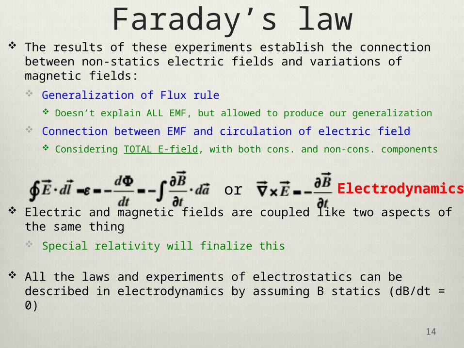
Faraday’s law The results of these experiments establish the connection

between non-statics electric fields and variations of magnetic fields: Generalization of Flux rule

Doesn’t explain ALL EMF, but allowed to produce our generalization

Connection between EMF and circulation of electric field Considering TOTAL E-field, with both cons. and non-cons. components

Electric and magnetic fields are coupled like two aspects of the same thing Special relativity will finalize this

All the laws and experiments of electrostatics can be described in electrodynamics by assuming B statics (dB/dt = 0)

or Electrodynamics!

15

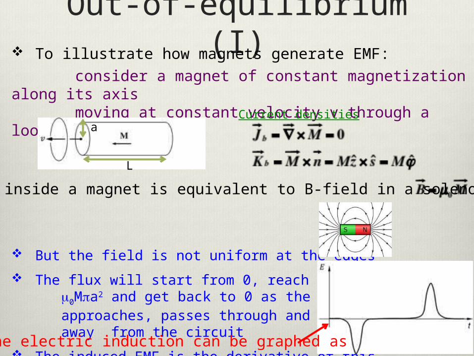
Out-of-equilibrium (I) To illustrate how magnets generate EMF:

consider a magnet of constant magnetization along its axis moving at constant velocity v through a loop wire

But the field is not uniform at the edges

The flux will start from 0, reach a max of m0Mpa2 and get back to 0 as the magnet approaches, passes through and moves away from the circuit

The induced EMF is the derivative of this

The field inside a magnet is equivalent to B-field in a solenoid:

L

a

The electric induction can be graphed as

Current densities

16

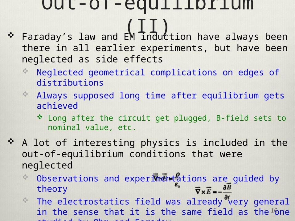
Faraday’s law and EM induction have always been there in all earlier experiments, but have been neglected as side effects Neglected geometrical complications on edges of

distributions Always supposed long time after equilibrium gets

achieved Long after the circuit get plugged, B-field sets to nominal

value, etc.

A lot of interesting physics is included in the out-of-equilibrium conditions that were neglected Observations and experimentations are guided by theory The electrostatics field was already very general in the

sense that it is the same field as the one studied by Ohm and Faraday

Two sources two undistinguishable components of E: E (cons.) generated by charges: E (non-cons.) generated by varying B-field:

In absence of charges, dynamics of E is analogous to that of B

Out-of-equilibrium (II)

Lenz’s law How do we know in which direction does the current

flow?

With motional EMF, we can use the right-hand rule as in magnetostatics

While it works in the case of an electromagnetic induction …

If dF > 0, I is clockwise

If dF < 0, I is counterclockwise

… it doesn’t make much sense in the situation of the third Faraday’s experiment because:

There are no moving free charges in a perpendicular B field

There are no cross products between two quantities

Lenz’s law is another rule to determine the direction of the current:

Nature opposes to a change of flux so generates a current to cancel the change of flux

17

See slide 15

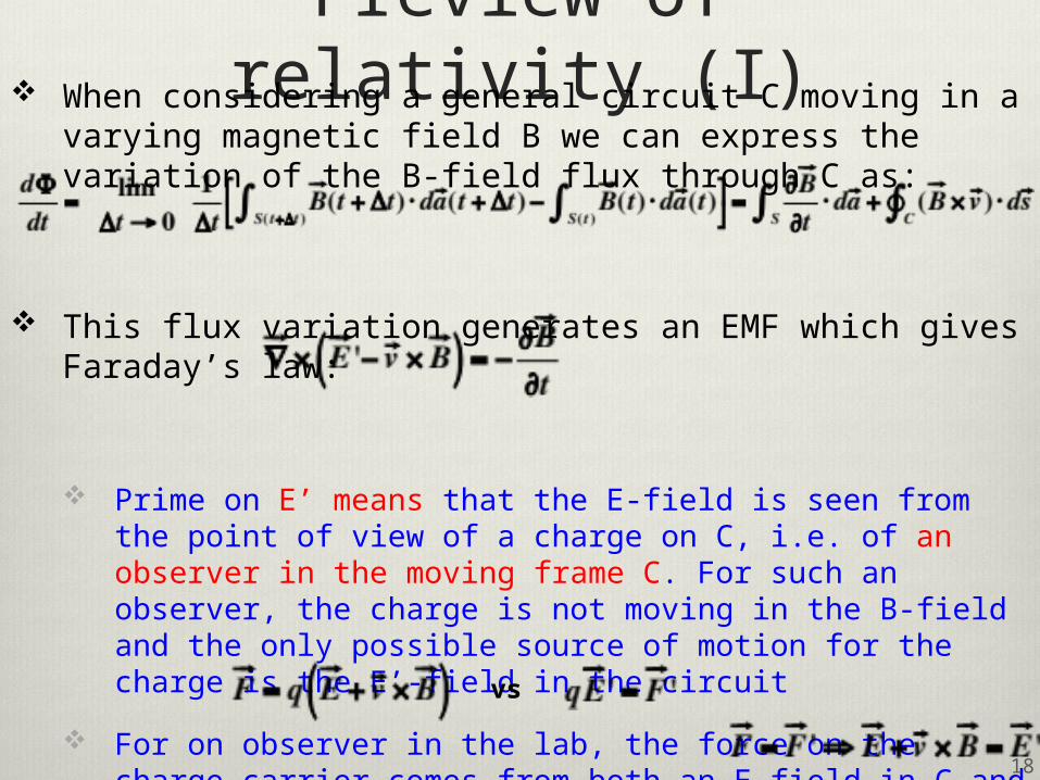
Preview of relativity (I) When considering a general circuit C moving in a varying

magnetic field B we can express the variation of the B-field flux through C as:

This flux variation generates an EMF which gives Faraday’s law:

Prime on E’ means that the E-field is seen from the point of view of a charge on C, i.e. of an observer in the moving frame C. For such an observer, the charge is not moving in the B-field and the only possible source of motion for the charge is the E’-field in the circuit

For on observer in the lab, the force on the charge carrier comes from both an E-field in C and the B-field (Lorentz force):

The force must be the same in all inertial frame

18

vs

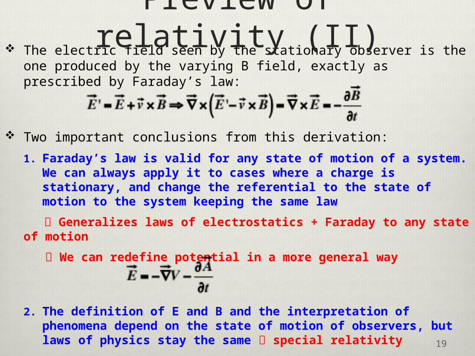
The electric field seen by the stationary observer is the one produced by the varying B field, exactly as prescribed by Faraday’s law:

Two important conclusions from this derivation:

1. Faraday’s law is valid for any state of motion of a system. We can always apply it to cases where a charge is stationary, and change the referential to the state of motion to the system keeping the same law

Generalizes laws of electrostatics + Faraday to any state of motion

We can redefine potential in a more general way

2. The definition of E and B and the interpretation of phenomena depend on the state of motion of observers, but laws of physics stay the same special relativity 19

Preview of relativity (II)

20

Inductance Faraday’s law says that a varying B-field generates an

EMF, and Biot-Savart’s law says that a current in a circuit produces a magnetic field. Putting these effects together:

A varying current in a circuit C generates an EMF in any circuit C’ in the vicinity of C, including C itself

The EMF generated by the varying current is characterized by the the concept of inductance

Auto-reactive effect of electromagnetic induction, similar to the mutual adjustment of P/M and E/B

The inductance is a property of a system as a whole This is what is handled in actual experiment and techno

applications Complementary to diff. equations that adopt a local point of

view

Have beneficial and detrimental practical effects on circuits

21

An analogy We already encountered a property describing systems of

conductors as a whole, which modifies the EMF of a circuit: the capacitance

By analogy, let’s try to find a linear relationship between a varying current and the generated EMF, for which the proportionality constant depends only on the geometry of the whole system

Strategy to achieve this:

1. Consider the flux of a B-field (the area is a geometric factor) Take the setup of the empirical Ampere’s experiment, but with I only in

C

2. Use Biot-Savart’s law to express the B-field in terms of the current I The factor multiplying I would be only geometrical

3. Apply Faraday’s law (differentiate I with respect to t)

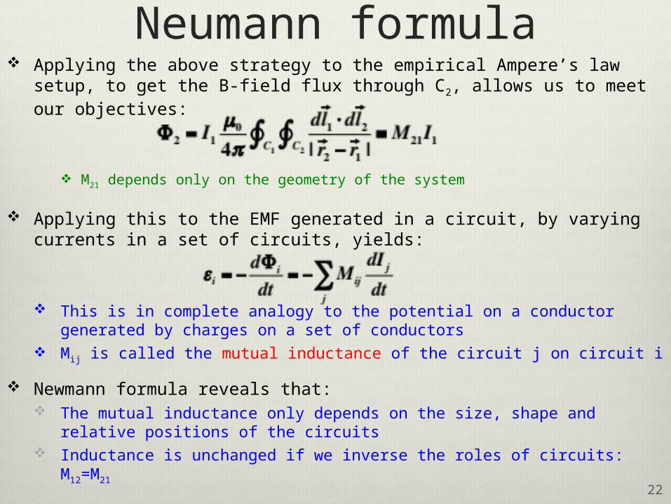
Neumann formula Applying the above strategy to the empirical Ampere’s law

setup, to get the B-field flux through C2, allows us to meet our objectives:

M21 depends only on the geometry of the system

Applying this to the EMF generated in a circuit, by varying currents in a set of circuits, yields:

This is in complete analogy to the potential on a conductor generated by charges on a set of conductors

Mij is called the mutual inductance of the circuit j on circuit i

Newmann formula reveals that: The mutual inductance only depends on the size, shape and

relative positions of the circuits Inductance is unchanged if we inverse the roles of circuits: M12=M21

22

23

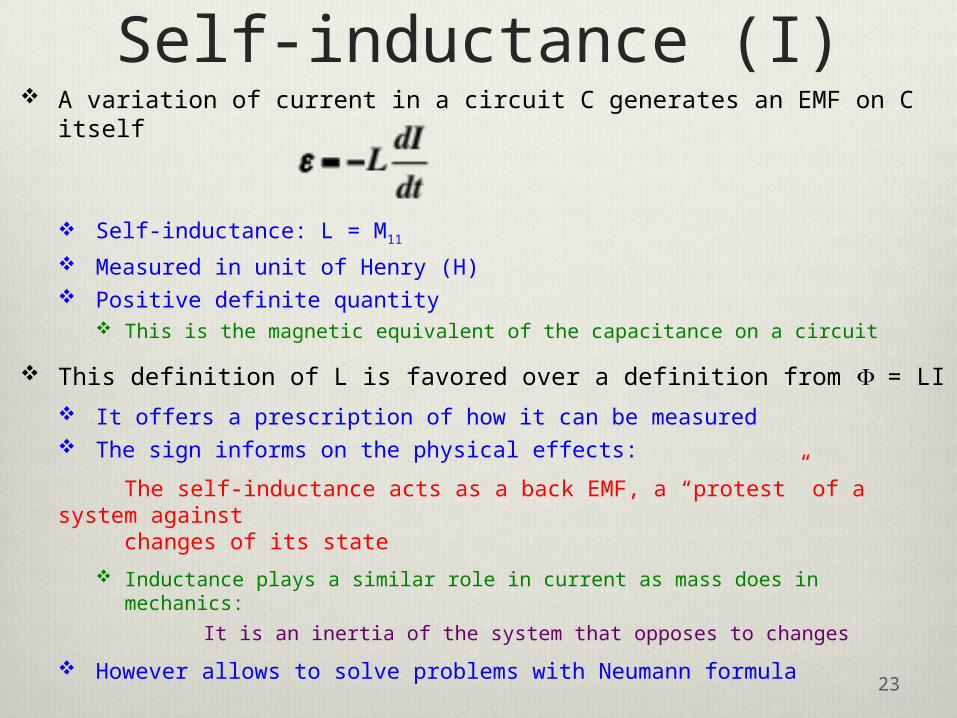
Self-inductance (I) A variation of current in a circuit C generates an EMF on C itself

Self-inductance: L = M11

Measured in unit of Henry (H) Positive definite quantity

This is the magnetic equivalent of the capacitance on a circuit

This definition of L is favored over a definition from F = LI

It offers a prescription of how it can be measured The sign informs on the physical effects:

The self-inductance acts as a back EMF, a “protest” of a system against changes of its state

Inductance plays a similar role in current as mass does in mechanics:

It is an inertia of the system that opposes to changes

However allows to solve problems with Neumann formula

24

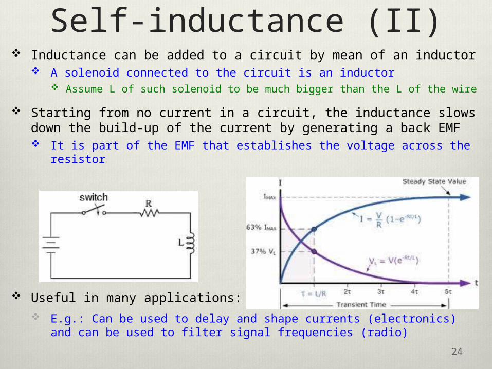
Inductance can be added to a circuit by mean of an inductor A solenoid connected to the circuit is an inductor

Assume L of such solenoid to be much bigger than the L of the wire

Starting from no current in a circuit, the inductance slows down the build-up of the current by generating a back EMF It is part of the EMF that establishes the voltage across the

resistor

Useful in many applications:

E.g.: Can be used to delay and shape currents (electronics) and can be used to filter signal frequencies (radio)

Self-inductance (II)

Energy of a B field (I) The B-field does no work on a charge, but it acts on a system,

exerts a force, and energy must be provided to charges to create it The B-field is expected to store energy

We can’t use the same approach as the one used in electrostatics to estimate this energy, but we will use Faraday’s law

Strategy: use the fact that the E-field, produced as B builds up, generates a force, which can do a work that can be used to get UB

We can estimate the work done by a battery against the back EMF in order to reach a steady current and the maximal B-field in the inductor;

This work is reversible because it will be released from the inductor when the circuit will be switched off;

We cannot use the energy given by the battery because, during the build-up, part of the energy supplied by the battery also gets dissipated as heat

25

26

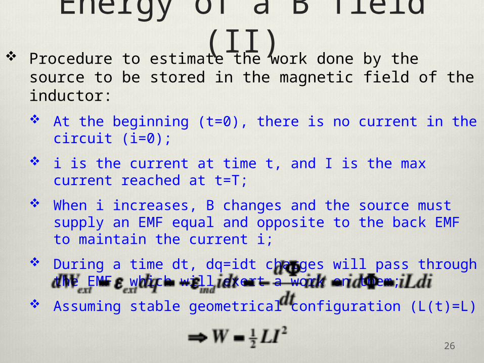
Procedure to estimate the work done by the source to be stored in the magnetic field of the inductor:

At the beginning (t=0), there is no current in the circuit (i=0);

i is the current at time t, and I is the max current reached at t=T;

When i increases, B changes and the source must supply an EMF equal and opposite to the back EMF to maintain the current i;

During a time dt, dq=idt charges will pass through the EMF, which will exert a work on them;

Assuming stable geometrical configuration (L(t)=L)

Energy of a B field (II)

Where is the energy stored?

This work, needed to yield the B-field in the inductor, can be expressed in terms of the vector potential and the current:

This can be generalized to any current density

The energy seems to be stored in the current density distribution!

But… using Ampere’s law, we can express the current density in terms of the magnetic field

The energy is stored in the magnetic field The situation is completely analogous to what we saw for UE 27

or