AGRICULTURAL RESEARCH REPORTS

Photosynthesis of l~af canopies

C. T. de Wit

663

Photosynthesis of leaf canopies

Offset reprint.. 1966

©Centre for Agricultural Publications and Documentation, Wagenirtgen, 1965 No part of this book m~y be reproduced and/or pUblished irt any for.rh, photoprint1 micro­film or any other means without written permission from the publishers.

C. T. de Wit

Institute for Biological and Chemical Research on Field Crops and Herbage, Wageningen

Photosynthesis of leaf canopies

1965 Centre for Agricultural Publications and Documentation

Wageningen

Agricultural Research Reports no. 663

Contents

1 SYNOPSIS ••. 3

2 INTRODUCTION 4

3 SOME BASIC DATA ON LIGHT AND PHOTOSYNTHESIS . . . . . . . . . . . . 6 3.1 Amount of diffuse and direct light on days with clear and overcast skies 6 3.2 Photosynthesis of single leaves. . . . . . . . . . . . . . . . . . 8

4 LEAF DISTRIBUTION FUNCTIONS . . 11 4.1 A classification of distribution functions 11 4.2 Spherical leaf distribution 12 4.3 A measuring method. I 3

4.3.1 Field crops 13 4.3.2 Pastures . . . 13

5 LIGHT DISTRIBUTION FUNCTIONS . . . . . . . . . . . 16 5.1 Canopies with leaves of the same inclination . . . . 16 5.2 Canopies with arbitrary leaf distribution functions . I 9 5.3 Canopies with spherical leaf distribution 19 5.4 A measuring method . . . . . . 21

6 PENETRATION OF LIGHT INTO CANOPIES 23 6.1 Canopies with horizontal leaves . 23 6.2 Canopies with arbitrary leaf distribution 24 6.3 Scattering of light in canopies . 24 6.4 Estimation of canopy density . . . . . 26

7 COMPUTATION OF THE PHOTOSYNTHESIS OF CANOPIES . . . . . . 27 7.1 Basic procedure . . . . . . . . . . . . . . . . . . . . 27 7.2 Effect ofrestricted transfer of carbon dioxyde to the canopy 29 7.3 Daily total of photosynthesis . . . . . . . . . . . . . 31

8 PHOTOSYNTHESIS RATE OF CANOPIES UNDER V ARlO US CONDITIONS 33 8.1 Canopy density . . . . . . . . 33 8.2 Leaf-area index and age of leaves . . . . . . . . . . . 35

8.3 Scattering coeffiCient . . . . . . . . . . . . . . 8.4 Fractioh of diffuse light . . . . . . . . . . . . ~t5 Inclination of the sun arid ctHtdition of the sky • •. • . 8.6 Photosynthesis functiorl . . . . . . . . . . • • 8. 7 Concentration and transfer of cat bon dioxyde . . 8.8 Leaf disttibution function . . . . , . . . : . .

9 DAILY tOtALS OF PHOTOSYNtHESIS UNOER VARIOUS CONDITIONS

9.1 Climate in Wagenirtgen and Kabanyolo .. 9.2 Sorrte widely diffetent canopies . . . . . • l

9.3 Candpies with spherical leaf disttibutiotl . , . .

10 FoRtRAN PROGRAMS. .... . . LitERATURE. • • • • •

2

36 31 37 39

j l 40 40

44 l ••• l • 44

...

45 47

51

56

1 SYNOPSIS

The photosynthesis rate of a leaf canopy depends on the reflection, the transmission and the photosynthesis function of the leaves, the position of the leaves with respect to the horizontal surface and each other, the leaf area per unit soil area, the amount of diffuse and direct light, the height of the sun and the resistance against the transfer of carbon dioxyde from the bulk of the air to the canopy. The development of a procedure to calculate the effect of these factors imposed

mainly geometrical problems, which were solved in such a way that the actual calcu­lating of canopy photosynthesis can be executed by means of a computer. The solution has been carried on to the stage where the daily photosynthesis of a canopy with known characteristics can be computed for any time and place on earth from the relevant meteorological data.

The calculating procedures have been used to study the relative importance of the above variables under various conditions. The results for a standard set of conditions have been summarized in such a way that it is possible to estimate the daily photosyn­thesis at any time and place for a wide range of photosynthesis functions without computer.

3

2 Introduction

The subject matter of this paper is most suitably introduced by a graph (figure I) out of BoYSEN JENSEN's (1932, 1949) classical papers on dry matter production of plants and by giving a condensed version of his views on photosynthesis in plant communities.

The influence of light intensity on the photosynthesis of a leaf of Sinapis alba at 20°C and normal air is given by curve 1 in figure I. The compensation point lies at 750 "Boysen-Jensen lux", and the photosynthesis increases more or less linear with the intensity of light, until a maximum is reached at about 14000 "Boysen-Jensen lux", that is about 30 percent of the average light intensity at a horizontal surface in the middle of the day. Obviously, a horizontally placed leaf is unable to utilize the full daylight completely.

But in a canopy of leaves the leaf area is larger than the soil area and the leaves are slanting, so that a great part of the leaves is exposed to an intensity of light amounting only to a certain fraction of the daylight and a far better utilization of the light may

~~-2-so cm2 hr

I 3

10

4

Fig. 1. Photosynthesis rates a/Sinapis alba. I. Rate per unit leaf area for one leaf: 2. Al'erage rate per unit leaf area in a

canopy with a lea.rarea index o/3.4. 3. Rate per unit soil area, covered by a canopy with a leaf-area index of3.4. "B. J. Lux" is a light intensity unit which was tised by BoYSEN JENSEN.

Datafrom BoYSEN JENSEN (1932,1949).

result. Therefore, the relation between the photosynthesis and light intensity is differ­ent from the one for horizontal leaves. This was indeed found. Curve 2 in figure l, represents the relation between the light

intensity at the top of a canopy of Sinapis alba and the photosynthesis for leaves in this canopy, like curve 1 calculated per 50 cm2 leaf area and per hour. The respiration is the same in both cases but as the leaves in the canopy partly shade each other, the slope of curve 2 is far less steep than of curve I and the compensation point is therefore at a higher light intensity and light saturation does not occur in the range of intensities used. As the leaf area in the canopy was 3.4 times the soil area, the photosynthesis per 50 cm2 soil area (curve 3) differs from that of curve 2 by a factor 3.4. The slope of curve 3 is almost the same as the slope of curve 1 at low light intensities, but its compensation point lies at the same intensitiy of light as for curve 2. The canopy demands more light than the horizontal leaf to reach a positive result of photosynthesis but on the other hand it utilizes a far higher intensity oflight, although at very high light intensities the photosynthesis curve is expected to level off too.

This example shows that the photosynthesis of a canopy does not only depend on light intensity and photosynthesis function of the single leaves, but also on factors which affect the distribution oflight over the leaves of the canopy. The most important of these latter factors are the number and size of the leaves and their position with respect to the soil and to each other, the transmission and reflection of the leaves and the ratio between diffuse and direct light and the height of the sun. It has been recognized that it is practically impossible to determine the influence of

these factors on the photosynthesis of canopies by means of experiments and that the calculation of these effects imposes mainly geometrical problems. But the geometry appeared to be of such complexity that rather sweeping generalizations of different kinds have been introduced (MONSI and SAEKI 1953, NICHIPOROVICH 1954, 1961, DE WIT 1958, 1959) to limit the computational work. At present high speed computers are readily available, so that the lack of basic data

can be the only excuse for simplification, but not the cumbersomeness of the computa­tional work. Therefore, the problem has been studied again, but now in such a way that due attention is paid to details and that ultimately canopy photosynthesis can be computed for any possible combination ofleaf and canopy characteristics and meteoro­logical data.

The present report on this study is written in such a way that it can be read by any­one who is only interested in the approach, the underlying assumptions, and the results. All physical, mathematical and computational details are given in small print and can be skipped by anyone who is not specially interested in them. The liberal use that could be made of the IBM 1620 computer of the Agricultural Uni­

versity and the help of the Staff of the Computer Centre in Wageningen is kindly acknowledged.

5

3 Some basic data on light and photosynthesis

In any attempt to calculate the photosynthesis of leaf canopies under natural condi­tions, the amount of light arriving at the canopy surface and the photosynthesis of the leaves of the canopy must be known. The dependence of the amount of diffuse and direct light on the height of the sun

with clear and overcast skies was measured many years ago and can be compiled in a suitable form without undue difficulties. Information on the effect of environmental and endogeneous factors on the photo­

synthesis of leaves will be summarized here in a form suitable for the present purpose, but a critical survey of the subject is not given.

3.1 Amount of diffuse and direct light on days with clear or overcast skies

Based on the work of KLEIN (1948) and of KIMBALL and HAND (1921), FRITZ (1949) constructed nomograms from which the total global radiation in the visible region was obtained, depending on the height of the sun for a cloudless and dustless sky in the following way. The amount of precipitable water is about 10 mm on very clear days. The total global

radiation at this value was read from FRITz' diagram for various heights of the sun. The radiation fluxes were multiplied by 0.5 (compare VAN WnK, 1963) to obtain the incident light intensity within the phososynthetic active region of 400-700 m!J.. Curve 1 in figure 2 gives this light intensity as a function of the inclination of the sun. The ac­tllilllight intensities on apparently clear days ma:Y be up to 15 per cent lower, because of more precipitable water and more dust in the atmosfere. This will be accounted for in due course.

A part of the total global radiation comes directly from the sun and the other part is diffuse sky radiation. KIMBALL (MET. TABLES, 1951), suggests that about half of the radiation lost from incoming rays by scattering and diffuse reflection is finally received at the surface of the earth as diffuse radiation. Many estimates of diffuse radiation (KLEIN, 1948, BERNHARDT and PHILLIPS, 1958) are based on this assumption.

However, short wave radiation scatters more than long wave radiation so that the amount of diffuse sky light is underestimated in this way. The scattering of this light is more closely correlated to the scattering of the luminous flux. JoNES and ·coNt>IT (1948) calculated the illuminance of a.horizontal surface due to direct and diffuse light

\

6

at heights of the sun from 0 to 90 degrees (their table IV) from many measurements of KIMBALL and HAND (1921) on clear days. These values are used here to estimate which part of the light reaches the earth's surface as direct light and which part as diffuse light. The resulting amounts are given by curve 2 and 3 in figure 2. The light with overcast skies depends of course on the density of the clouds. A fair

assumption is that the light on overcast days is about 20 per cent of the light on very clear days as defined above, (compare DE VRIES, 1955) and that the sky brightness is uniform (curve 4). Light distribution under hazy conditions and under conditions of a partly clouded

sky is so variable that generalizations useful at this stage cannot be given. The bright­ness of the sky is highest opposite the sun and lowest at the zenith (KIMBALL, 1921).

incident light in tensity cal

crn2 min

0.8 -

0.6-

r 0.1.

0.2

3

0 .. .-=----'----'---·-j___I __ __L__ _ ___._ __ ....._ _ __...._

15 25 35 4S 55 65 75 85 ° inclination of sun IS

Fig. 2. Incident light intensity or the radiant energy within the wavelengths of 400 and 700 m!J.for various heights of the sun. 1. Total light with a very clear sky. 2. Direct light with a very clear sky. 3. Diffuse light with a very clear sky. 4. Total and diffuse light with an overcast sky. Data from KIMBALL (1921), KLEIN (1948), FRITZ (1949), MET. TABLES (1951) and VAN WDK (1963).

7

But the brightness of different sections of the sky is not measured as a routine, and anyhow is so variable (compare DoGNIAUX, 1954) that. at present the only reasona­ble assumption is that it is uniform. The relative contribution of each zone of the sky to the illuminance of the horizontal surface is then as given in table I.

Table 1. The relative contribution to the illuminance of the lwrizontal su1:(ace of /0 degree zonesji·om a sky with un({orm br(r;htness.

inclination (degrees)

rei. contr.

0

.030

to

.087

20 30 40

.133 .163

50 60 70 80 90

.174 .163 .133 .087 .030

lt is supposed with KIMBALL and HAND (1921) that the hemispherical sky surface of radius R is divided into elementary zones and that the inclination of these zones is IS. In that case the circum­ference is 2 ·7t' • R • cos(1s) and the width is R · d(Js), so that its area is 2 '1t' • R 2 ·cos( Is)· d(1s). When the sky brightness equal~ everywhere I, the illtiminance of the horizontal surface is

r:/2

f 2·TC· R2• COS(lS)•SJN(lS)· d(JS) (I)

()

By substituting the appropriate boundaries and by dividing with the factorTC· R 2, table I is obtained.

3.2 Photosynthesis of single leaves

The photosynthesis of leaves is expressed in units C02 absorbed per unit time and unit leaf area. Since the influence of respiration on dry matter accumulation is not studied here, true photosynthesis rates are considered, i.e. the uptake of C02 in the dark is taken as zero. The-photosynthesis rate of canopies is expressed here in kg Cl-I~O ha-1 hour-I, and it is therefore convenient to use the same units for the photosynthesis of single leaves. In general, the photosynthesis of leaves is given as a function of the incident light.

intensity. This intensity contains the fraction of light reflected and transmitted by the leaves. Since the calculations in this paper concern the amount of light absorbed by the leaves, the incident light intensities must be converted into absorbed light intensi­ties. Where ttansmission and reflection of the experimental material are not reported, this may be done by multiplying with 0.7-0.8, which is a fair estimate of light absorp­tiot1 by normal leaves (section 6.3).

The functional relation between photosynthesis and absorbe'd light intensity can be given in tabulated form and photosynthesis at any absorbed light intensity may be found by interpolation. This procedure has the disadvantage of taking considerable storage space in the computer, especially when it is supposed that the relation is not the same for all the leaves of the canopy.

8

Fortunately, (RABINOWITCH 1951, MoNTEITH (in EVANS, 1963)) the photosynthesis function of leaves can be represented satisfactory by the equation

A = H · (H + HH)-1. AMAX (2)

where A and Hare the photosynthesis rate and the absorbed light intensity, AMAX is the photosynthesis at very high light intensities and HH the light intensity at which half of the maximum photosynthesis occurs. The equation can also be written in the following way

A = H · (H + AMAX · E-1)-1 · AMAX (3)

In this case E ( = (A/H) H~o = AMAX/HH) is the efficiency of photosynthesis. Values of AMAX, HH and E, calculated from GAASTRA's (1959) data for sugar-beet

leaves with normal C02 concentrations at the leaf surface are about 20 kg CH20 ha-1

hour-1, 0.056 cal cin-2 min-1 and 357 (kg CH 20 ha-1 hr-1) f (cal cm-2 min-1). The

photosynthesis for leaves of several plant species is about the same as for sugar beets, but it may differ considerably for other agriculturally important species in one or the other direction (LARCHER, 1963). The assumption that all leaves of a canopy have the same photosynthesis function suffices as long as there are only random variations between the leaves. However, it may be that the photosynthesis function varies with the depth of the leaf within the canopy. For instance, according to HoPKINSON (1964), the photosynthesis rate of the 2nd leaf of a cucumber plant dropped with 75 per cent from the 17th to the 33rd day of life. A similar large effect was observed by SAEKI (1959) with buckwheat, but the effect of leaf age was much smaller in case of green gram. HEINICKE and HOFFMAN (1933) also found a small effect of the age of apple leaves. The change of the photosynthesis function with depth that may result is illustrated by

a series of measurements of SAEKI (1959), summarized in figure 3. These data concern the photosynthesis function of Celosia cristata at different positions along the stem, the leaves being numbered upward from the lowest one alive. Only the lowest leaf

mg CO:z

50 cm2 hr

10

5

0 ·--~--·-____L _____ l ___ __j

20 40 kilolux

-2

Fig. 3. Photosynthesis function of leaves of Celosia cristata numbered from the lowest leaf upwards. Data from SAEKI

(1959).

9

showed yellow discoloration. The maximum value of the photosynthesis rate (AMAX)

appears to decrease with increasing depth, but the light intensity at which one half of the photosynthesis occurs (HH) appears to be the same, throughout. GAAST~A (op. cit.) and others showed that the efficiency E (equation 3) is practically

independent of the C02 concentration of the air, but that AMAX is proportional with this concentration in the range of 0-500 ppm. Accordingly, decreases in carbon-diox­yde concentration at the c~nopy level due to a limited exchange from carbon dioxyde from the bulk of the air to the air in the canopy must be taken into account. The leaves of a canopy are not of the same temperature, because they are differently

exposed to radiation and wind. Fortunately, it has been shown repeatedly (GAASTRA,

op. cit.) that within a rather wide temperature range the photosynthesis function is 110t affected by temperature, provided the C02-concentration is not above normal.

Moss (1964) studied the photosynthesis function of leaves when illuminated from above or below. This did not make any difference with gramineous species because the chloroplasts are uniformly distributed throughout the mesophyll. The leaves of dico­tyledonous plants showed higher photosynthesis when illuminated at the side of the palissade cells, because these contain most of the chloroplasts. But with leaves of both classes photosynthesis was highest when illuminated from both sides, because then the light was more evenly distributed over the chloroplasts.

GAASTRA (1964) made it clear that neither the efficiency E nor the maximum photo­synthesis are affected, so that the effect may occur at intermediate light intensities only. Because it is still difficult to obtain estimates of the constants in equation 2 and 3, which are accurate enough for further calculations, the rather small effects of the direction of illumination are negle~ted at present.

4 Leaf distribution functions

Among other factors, the light received by a canopy depends on the position of the leaves in space. This position is completely determined by the azimuth and the inclina­tion of the plane through each leaf element. It will be shown at first that the leaves of a canopy have in general no preferred azi­

muth direction so that their positions are completely characterized by the cumulative frequency distribution of the inclination of the leaves. Then, a classification of these di~tribution functions is given, and one function of some theoretical importance is derived. Subsequently, a method of measuring the distribution function of the leaves of a canopy is discussed, and functions for canopies of different plant species are given.

4.1 A classification of distribution functions

According to some measurements of NICHIPOROVICH (1961), the leaves of a canopy have not a preferred azimuth direction (table 2).

Table 2. Percentage of leaves in90 degree sections facing the four cardinal points (NICHIPOROVICH, 1961).

wheat corn

South 26 23

West 26 27

North 23 24

East 25 26

Our experience points in the same direction. Of course, leaves of some species tend to maintain the same position with respect to the sun or are oriented because of wind. But it is unrealistic to incorporate the possibility of this orientation in the calculations because orientation in most cases is not pronounced, the knowledge of the relative brightness of the sky sections is very limited (section 3.1) and the effect of seemingly large differences in leaf position on canopy photosynthesis may be surprisingly small, as will be shown in section 8.8. It suffices therefore to characterize the positions of the leaves of a canopy only by the cumulative frequency distribution of the inclination of the leaves.

Such distribution functions are conveniently represented by plotting the cumulative frequency of occurrence of the inclinations against the inclination, ranging from 0° for a horizontal leaf to 90° for a vertical one. This is done in figure 4a. It is convenient to distinguish canopies of four types, according to their leaf distribution. Horizontal

11

cum.freq. of I L a 1~----------------~=-~

0.8

0.6

0.4

0.2

90, lL

Fig. 4. a. The four types of leaf distribution functions. b. The spherical leaf distribution/unction.

cum. freq. of IL b 1~------------------~~

0.8

0.6

0.4

0.2

goo lL

leaves are most frequent in planophile canopies, and vertical leaves occur most in erectophi/e canopies. The leaves in p/agiophile canopies are most frequent at some oblique inclination, whereas those in extremophi/e cartopies are the 1east frequent at oblique inclinations.

4.2 Spherical leaf distribution

An erectophile leaf distribution function of some interest is given in figure 4b. This is a theoretical distribution which is obtained by supposing that the relative frequency Qf leaf inclinations is the same as the relative frequency of the inclinations of the surface elements of a sphere. The leaves of grasses, small grains and corn manifest according to NICHIPOROVICH (1961), this spherical distribution, but this is only partly confirmed by our measurements (section 4.3).

When IL is the ihclination of a leaf (figure 11)

rt/2

1 = P[!!:< 7t/2] = J w·2•7t•A•R·(2·7t·R2)-1 ·d(IL) = 0

rt/2 r:/2

= J w·stN(IL)·u(IL) = w· [-cos(IL)) = w ' 0

0

holds in the case of a spherical distribution, so that the cumulative distribution function of IL is

P[IL < !~] = I - COS(IL)

12

'(4)'

4.3 A n1easuring n1ethod

A straightforward method to measure distribution functions has been applied by NICHIPOROVICH ( 1961 ). The instrument used is a leaf graduator consisting of two pro­tractors, l em apart and a free moving pointer at an axis through the centres. The base of the protractor is kept parallel to the leaf or leaf section so that the angle between the horizontal surface and the leaf can be directly read from the position of the pointer along the protractor. After some training it is possible to measure leaf angles with some accuracy. If different sections of the same leaf have different angles, as is for in­stance the case with corn, the angle of leaf sections of about the same size is measured. Measuring the angle of about 400 leaves or leaf sections suffices to obtain reasonable smooth and reproducable distribution functions. To characterize a canopy, one may stratify the crop and determine the leaf distribu­

tion function of each layer by random sampling within this layer. But, as will be shown (section 8.8), the effect of leaf distribution on photosynthesis does not justify the large amount of work associated with stratified sampling. Instead, a suitable num­ber of plants or small crop areas are selected at random and the angle of each leaf or leaf section of the plants or in the crop areas is measured.

4.3.1 Field crops

Leaf distribution functions for several well developed field crops are given in figure 5. The leaf distribution of rape seed (Brassica napus, var. oleifera) was slightly plagio­

phile until after flowering. During seed formation much of the light is intercepted by the green pods, but no method has been developed to obtain distribution functions for cylindrical objects. The leaf distribution functions of white clover and potatoes are about the most plano­

phile distributions observed by us and by NICHIPOROVICH (1961). The leaf distribution of sugar beets is plagiophile, during the whole growing period.

Canopies of corn and small grains are according to NICHIPOROVICH (1961) more or less spherical (compare figure 4b). The present observations confirm this for rye, but in case of corn plagiophile canopies are found.

4.3.2 Pastures

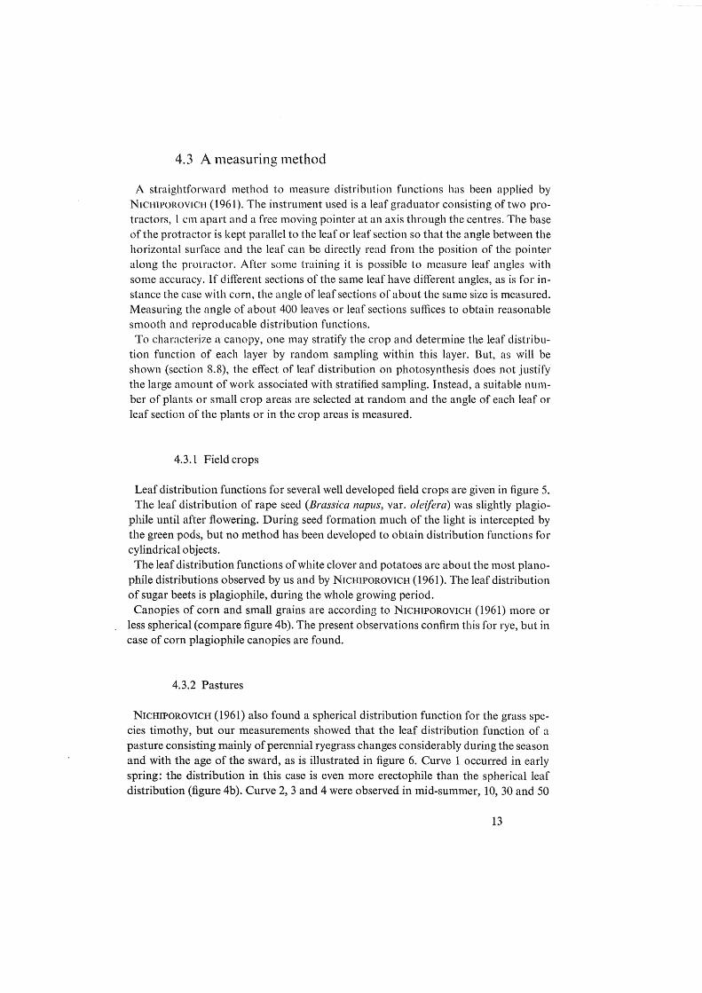
NICHIPOROVICH (1961) also found a spherical distribution function for the grass spe­cies timothy, but our measurements showed that the leaf distribution function of a pasture consisting mainly of perennial ryegrass changes considerably during the season and with the age of the sward, as is illustrated in figure 6. Curve 1 occurred in early spring: the distribution in this case is even more erectophile than the spherical leaf distribution (figure 4b). Curve 2, 3 and 4 were observed in mid-summer, 10, 30 and 50

13

c:um. freq. of lL 1

rope 1. Apr. 27 2. May 12

0.8 (flog leaf) 3. May 29

(heading)

0.6

1. Apr. 20

0.4 2. Apr. 27 0.4 3. May 12

(flowering)

0.2 0.2

0 0 0 30 60 goo 0 30 60 goo

IL IL

white clover potato

0.8 0.8

0.6 1. May 28 2. June17

(flowering )

0.4 August 21 (flowering)

0.2

0 0 30 60 goo 30 60 goo

IL IL

sugar beet corn

0.8

1. July 2 0.4

1. June 18 2. July 13 2. July 17 3. July 28 3. oct. 1

0.2 4. oct. 1 0.2

0 30 60 soo 0 30 60 soo

ll tL

Fig. 5. Leaf distribution functions for well developed canopies of some common agricultural spec1'es.

14

cum. freq. of IL 1.0 .....---------------.

30 60 goo 30 60 goo

IL IL

perennial rye-grass

curve age in days measured kg/ha 30 May 6

2 10 June 10 1300 3 30 .. 10 6000 4 50 .. 10 8800 5 10 Aug. 21

6 20 .. 21 2600 7 40 .. 21 5000 8 60 .. 21 6300

Fig. 6. Leaf distribution functions of perennial ryegrass pastures under various conditions.

days after mowing and after a liberal N-application. The 10 day old grass is again extremely erectophile, but the older grass tends to hang over, so that at an age of 50 days an obviously planophile distribution is obtained. The same pattern is observed during late summer (curve 5-8), the distributions being shifted somewhat in the plano­phile direction.

15

5 Light distribution functions

The light of the sun falling on a canopy is intercepted by leaves at various angles to the direction of this light. To calculate canopy photosynthesis it has to be known what fraction of the light is intercepted at what angles. The incident light interisity on a l~af due to direct light is proportional to the sine of the angle (Ls) between the leaf ~nd the rays of the sun. Therefore, it is most convenient to express the light distribution in . terms of the cumulative frequency distribution of intercepted light as a function er SIN (LS).

The putpose is now to develop a general method to obtain light distribution functions from leaf disttibtdion functions. This is done in two steps. At first a cal~ulation proce­dure is given to obtain the light distribution function in canopies with leaves of one in·

· clination. This method is used to calculate such distribution functions at sun and leaf itt~Urtati~hs af 5, 15, .......... , 85 degrees in all 81 possible combinations. These distri-lYt:iti()rt functions are used agairt to calculate light distribution functions for any desired leaf distribution and arty height of the sun. The light· distribution function for a canopy with spherical leaf distribution is also

discussed afld a method is given to measure directly light distribution functi-orts.

5.1 Canopies with leaves of the same inclination

Even in canopies with leaves of the same inclination the light is intercepted at various angles. For instance, with an inclination of the leaf and the sun of 60° and 30°, respec­tively, some light is intercepted by leaves perpendiculary to the rays of the sun, some by leaves almost parallel to these rays, while some light is intercepted by the under­side of the leaves. The calculation of the relative amounts of light intercepted at various angles is a straightforward geometrical problem.

'the line a in figure 7a is the intersection of the soil surface and a plane through a leaf or l~i:afsection. 'the line ts is in the direction of the sun. The angles IS, IL, DA and LS are the Inclirtations of the Sun, the Inclination of the Leaf, the Difference between the Azimuths of the leaf and the sun and the angle between the Leaf and the rays bf the Sun, respectively. The angle LS must be expressed in the other angles. The points sz and sh are the projections of s on both planes. Line a is perpendicular to the plane szssh because ssz and ssh are perpendicular to the plarte of the leaf and of the soil surface. Figure 7b is the same as figure 7a, but fot the position of the plane Szssh, which is now hG>ti~ontal, and the addition of point Q.

Now it is easily seen that on one hand SSi = TS·(SlN(ts)·coS(IL) + CoS(IS)·SIN(IL)·SIN(t>A))

16

leaf plane

a sun

Fig. 7. Illustration of the calculation of the light distribution/unction.

and on the other SSl = TS•SIN(LS) so that

b

T l eat plane

SIN(Ls) =A+ B·SIN(DA) (5) with A = SIN( IS)· COS(IL) B = COS(IS) • SIN(IL)

The light is parallel to theleafwhensiN (Ls) = 0, thatis when DA =ARCSIN (-A/B). Forlarger values of DA, the light falls on the underside of the leaves, and for smaller values of DA on the upperside. If IS is greater than IL, no light falls on the underside of the leaves. In this case the value -A/B is smaller than minus one, so that ARCSIN (-A/B) does not excist. To distinguish between light falEng on the upperside and on the lowerside of the leaves, the boundary angle DAO =ARCSIN (-A/B) fons < IL and DAO = -1t/2 foriS > IL (6) is introduced.

The amount of light intercepted by the leaves in a small azimuth interval is proportional to the size d (DA) of this interval, since it is assumed that the leaves do not have a preferred azimuth direction. This amount of intercepted light is also proportional to the projection of the surface elements in the direction of the sun, that is with SIN (LS). If P [ L at SIN(.!:-§)< SIN (Ls)] is again the probability that a light ray is intercepted by a leaf with a sine of its angle to the light equal or smaller than SIN (Ls), 1 =P(LatSIN(~)< 1] = the probability oflight on underside + probability on upperside =

DAO rt/2

= (- f SIN (LS) · d (DA) + f SIN (LS) • d (DA)) · W = -rt/2 DAO

17

DAO -r;f'2

= (- J (A+ B·SIN (DA))·d (DA) + J (A+ B·SIN (DA))·d (DA))·W =

--:t/2 DAO = (-2·A·DAO + 2·n·cos(DAO))·W so that P ( L at SIN(~)<; (A + B ·SIN (DA))] =

= (n·cos(oA)-A·(rr/2 + DA))·w and

forDA < DAO

= (B • (2 · COS(DAO)- COS (DA))- A· (2 · DAO + rr/2- DA)) · W for DA > DAO with

(7)

W = (2·B·COS(DA0)-2"A'DAO)-l (8) The calculating pro9edure is given in program 1 (section 10). Arbitrary values of IS and IL are read

and the appropriate values of A, B and w are calculated at stage 1. The light distribution function for SIN (Ls) = -0.9, -0.8, .......... , +0.9 is calculated at stage 2. By neglecting the difference between light interception by the upper- and by the underside of the leaves (section 3.2), this light distribution function is transformed in one for SIN (Ls) = 0.1, 0.2, .......... , 0.9 at stage 3.

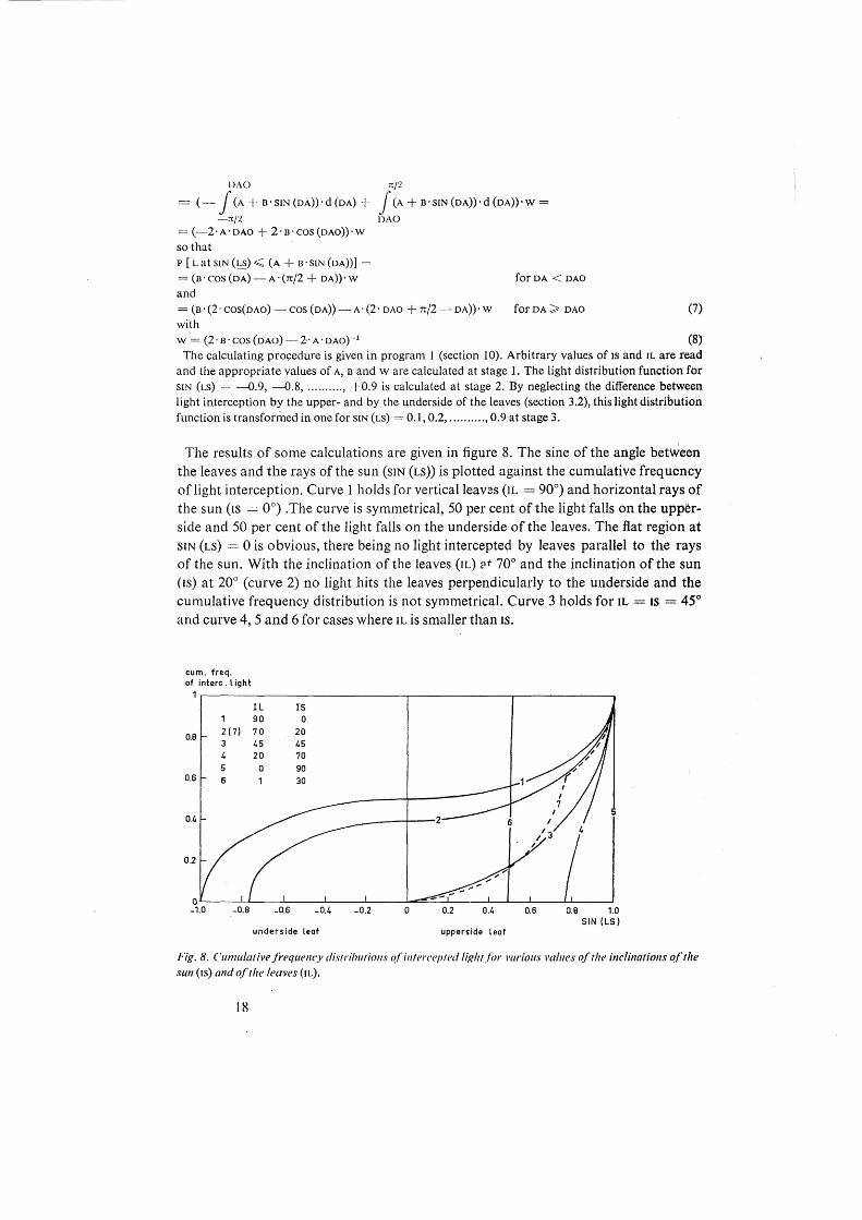
The results of some calculations are given in figure 8. The sine of the angle between the leaves and the rays of the sun (siN (Ls)) is plotted against the cumulative frequency of light interception. Curve 1 holds for vertical leaves (IL = 90°) and horizontal rays of the sun (Is = 0°) . The curve is symmetrical, 50 per cent of the light falls on the upper­side and 50 per cent of the light falls on the underside of the leaves. The flat region at SIN (Ls) = 0 is obvious, there being no light intercepted by leaves parallel to the rays of the sun. With the inclination of the leaves (IL) ::tt 70° and the inclination of the sun (Is) at 20° (curve 2) no light hits the leaves perpendicularly to the underside and the cumulative frequency distribution is not symmetrical. Curve 3 holds for IL =IS = 45° and curve 4, 5 and 6 for cases where IL is smaller than IS.

cum. freq. of interc. light

1r--------------------------~------------~----~--~~

0.8

0.6

0.1,

0.2

-0.8

IL 90 70

-0.6

IS 0

20

-0.1,

underside leot

~0.2 0 0.2 0.1, 0.6 o.e 1.0 SIN (LS)

upperside leof

Fig. 8. Cumulative frequency distributions o./'intercepted litdtt.f£n· J'arious l'tliues oftlu! inclinations of the sun (Is) and of the leaves (IL).

18

It has been shown in sectio!l 3.2 that it is not feasable to distinguish between upper and underside of the leaves, so that the sign of SIN (Ls) is eliminated by subtracting the cumulative frequency for SIN (Ls) = -0.1 from that for SIN (Ls) = + 0.1 and entering the result on the ordinate of SIN (Ls) = + 0.1 and so on. This is done for curve 2. The resulting curve 7 is discontinuous at SIN (Ls) = SIN (70- 20) = 0.77, because below this value light is intercepted by the upper and undersides of the leaves and above this value only at the uppersides. The light distribution functions for IS and IL in all81 possible combinations of 5, 15,

25, .......... , 85° have been computed and are used as a basis for calculating light distri­bution functions for any other canopy.

5.2 Canopies with arbitrary leaf distribution functions

The light distribution function for an arbitrary leaf distribution function and an arbi­trary inclination of the sun can be calculated by numerical methods. These are based on the principle that the light intercepted by leaves in any leaf inclination class is pro­portional to the number ofleaves in this class and to the projected area in the direction of the sun of one unit leaf area of this class.

The calculating procedure is summarized in program 2 (section 10). At stage 1, the nine light distri­bution functions for one inclination of the sun and 9 inclinations of the leaf (section 5.1) are read. Then, the area of the projection of one unit leaf area in the direction of the sun (oP) is calculated. At stage 2 the cumulative frequency distribution of leaf inclinations is read and the light distribution functions for this particular leaf distribution and inclination of the sun are obtained for SIN (Ls) = 0.1, 0.2, .......... , 0.9. The mean area of the projection of one unit leaf area in the direction of the sun (oPG) is obtained at stage 3. This program must be used nine times with the appropriate inputs to obtain the light distribution

functions at inclinations of the sun of 5, 15, .......... , 85 degrees.

The result of some calculations for the four leaf distribution functions of figure 4a are given in figure 9. The difference between the four distribution types is considerable and, at least quali­

tatively, easily understood. The accuracy obtained by dividing the traject for each variable into nine or ten classes, as in this case, is adequate compared with the accura­cy of measuring leaf distribution functions (section 4.3).

5.3 Canopies with spherical leaf distribution

The light distribution function for this canopy is presented in figure 10. This canopy is the only one with a light distribution function independent of the inclination of the intercepted light. This follows directly from the definition of the spherical leaf distri­bution in section 4.2.

19 J

cum. frtq. of interc.ligh t

1.0 ,.-------·---- ~~

IS 0,~• /5 ..... /

Plonophile canopy

0.8 /0 &

./ I I '·5 / j ./ I .

0.6

0.4

0.2 I . / / ,as"'• .--· .--·

0~-+-=4~~~~--~·---~·-·---~'-----~----~ 0 0,2 0.4 0.6 0.8 1.0

SIN (LS)

1.0

0.8

0.6

0.4

0.2

cum. freq. of interc. light 1.0r----

Erl!ctophlle canopy 0.8

0.6

0.4-

0.2

0 0

.,'·5 E,t,•moph;te <anopy ItS

·.;//. ./ · ..

/ . . . / ... • / •. a~· 0.2

~· .c.-• ...,.-•--~·-::::::7 .

0 ~.-- __ -1.~-~ .. .L-~· o.a 1.0 o. o.2 o.4 o.6

51pN.e(• ... , to

SIN (LS) " .. ' . . .

O.'l 0.4 0.6

Fig. 9. Light distributions functions for inclinations of the su11 (Is) of 5,45 and 85 degrees and tht leo/di~ .. tributionfunctions presented in figure 4a.

cum. freq. of interc. light 1.0r----

0.8 .

0.6 -

0.1. -

0.2

0.2 0.4 0.6 0,8 1 SIN (LS)

Fig. 10. Light distributionfunclioll.for a canopy with e1

sphericalleafdistribillioll. ·

20

The light distribution function is independent of the inclination of the sun in case of a spherical leaf distribution, so that it suffices to consider the situation of figure ll only with the sun in vertical posi­tion. The amount of intercepted light at an angle LS is proportional with the amount of surface element at this angle, that is with cos (Ls), and with the projection of these surface elements in the direction of the sun, that is with SIN (Ls). IfP [ L at SIN(~)< SIN (Ls)] is the probability that a light ray is intercept­ed by a leaf of which the sine of the angle to the light ray is equal or smaller than SIN (Ls), then 1 = P [LatSIN(!:-§) <:; 1) =

= W'SIN(LS)·COS(LS)·d(LS) = rr/2

= w· [SIN2 (LS)) = W 0

so that P ( L at SIN(~)<;; SIN (LS)) = SIN2 (LS) which is the function given in figure 10.

(9)

Fig. 11. Illustration of the calculation of the light distri­bution function for the spherical leaf distribution.

5.4 A measuring method

It may be that the leaf distribution function changes with the depth of the leaves in the canopy. Since most of the light is intercepted by the leaves at the top of the canopy, biassed results are obtained with the method of measuring leaf distribution functions advocated in section 4.3. Systematic errors of this kind are avoided by directly measur­ing the light distribution function. The instrument used for this purpose consists of two copper spheres of 15 mm, 10 centimeter apart, attached at a pole long enough to keep the spheres about 50 em above the canopy. This pole with the spheres is moved at random. When the sun shines, the left sphere casts a shadow on a leaf. The shadow of the right sphere is made to fall at the same time on a piece of cardboard with a milli­meter division. This piece of cardboard is held parallel to the leaf section which inter-

21

cepts the shadow of the left sphere. The length of the shadow can now be estimated and recorded. The sine of the angle between the leaf concerned and the sun rays is equal to the diameter of the sphere (in this case 15 mm) divided by the length of the shadow. By doing sufficient measurements for instance with the sun at an inclination be­

tween 40 and 50 degrees, a distribution function of light interception as given in figure 9, may be obtained for an inclination of the sun of 45 degrees. Of course, different distribution functions of light interception are obtained for different inclination classes of the sun. From these functions a leaf distribution function can be derived by a trial and error method based on the method discussed in section 5.2. It appeared that the angles of the leaves with a sine smaller than 0.5 are systematically

underestimated, but that reasonable leaf distribution functions can be obtained by lumping the leaves with a sine lower than 0.5 in one class, provided measurements at various inclinations of the sun are made. The computational work involved made it worthwhile to note the results directly on mark sensing charts and to carry out the rest of the work by means of the computer. Unfortunately, the weather in the Netherlands is so unpredictable that too many hours are lost by waiting for clear skies. In regions with more predictable weather the method may provide a good alternative of NICHI­POROVICH's method, the more so because a random sample of the leaves, contributing to light interception is obtained.

22

6 Penetration of light into canopies

If all light arriving at the leaves of a canopy came from one direction, knowledge of the light distribution function, the amount of leaves and the light intensity would suffi­ce to calculate how much light is received at each leaf position and from that the photo­synthesis of the canopy. But the amount of diffuse light arriving at a canopy is consi­derable, so that one leaf receives light from different directions and the penetration of the light out of these directions into the canopy has to be known to calculate how much light is received by each leaf of the canopy.

This penetration of light into canopies depends of course on the light distribution function and the angle of incidence. For instance, a canopy with vertical leaves inter­cepts the light from an almost horizontal direction at the tops of the leaves, whereas all light from the vertical direction penetrates to the soil surface, but this light is again intercepted by canopies with horizontal leaves. Light penetration depends also on the regularity of the distribution of the leaves

above the soil surface. For instance, light penetrates far less deep into a canopy con­sisting of horizontal leaves distributed so regularly that there are closed leaf layers, than into a canopy which consists of small leaves, distributed at random.

Light penetration is also affected by the reflection and transmission of the light inter­cepted by the leaves.

Starting with canopies with horizontal leaves, methods to calculate the penetration of light into canopies are developed.

6.1 Canopies with horizontal leaves

The penetration of light into canopies consisting out of layers with horizontal leaves which do not reflect or transmit light was treated by MoNSI and SAEKI (1953). They supposed that the area of the leaves in each layer is s (0 < s < 1) times the area of the soil. The fraction of light from the vertical direction penetrating through the first layer is then (1 - s) and the fraction of light penetrating through the Nth layer ( 1 - s) N. When the leaf-area index (that is the ratio of the leaf area and the soil area) is LAI the light that penetrates through the canopy is

I= IO. (1- s) LAI/S (10)

in which 10 is the amount of light arriving from the vertical direction at the canopy.

23

6 Penetration of light into canopies

If all light arriving at the leaves of a canopy came from one direction, knowledge of the light distribution function, the amount of leaves and the light intensity would suffi­ce to calculate how much light is received at each leaf position and from that the photo­synthesis of the canopy. But the amount of diffuse light arriving at a canopy is consi­derable, so that one leaf receives light from different directions and the penetration of the light out of these directions into the canopy has to be known to calculate how much light is received by each leaf of the canopy. This penetration of light into canopies depends of course on the light distribution

function and the angle of incidence. For instance, a canopy with vertical leaves inter­cepts the light from an almost horizontal direction at the tops of the leaves, whereas all light from the vertical direction penetrates to the soil surface, but this light is again intercepted by canopies with horizontal leaves.

Light penetration depends also on the regularity of the distribution of the leaves above the soil surface. For instance, light penetrates far less deep into a canopy con­sisting of horizontal leaves distributed so regularly that there are closed leaf layers, than into a canopy which consists of small leaves, distributed at random.

Light penetration is also affected by the reflection and transmission of the light inter­cepted by the leaves.

Starting with canopies with horizontal leaves, methods to calculate the penetration of light into canopies are developed.

6.1 Canopies with horizontal leaves

The penetration of light into canopies consisting out of layers with horizontal leaves which do not reflect or transmit light was treated by MoNSI and SAEKI (1953). They supposed that the area of the leaves in each layer iss (0 < s < 1) times the area of the soil. The fraction of light from the vertical direction penetrating through the first layer is then (1 - s) and the fraction of light penetrating through the Nth layer (1 - s) N. When the leaf-area index (that is the ratio of the leaf area and the soil area) is LAI the light that penetrates through the canopy is

I = IO. (1- s) LAI/S (10)

in which 10 is the amount of light arriving from the vertical direction at the canopy.

23

At the extremes= 1, the leaves are arranged in closed layers ofleaf-area index 1, and no light penetrates to the second layer of leaves. This mozaic leaf arrangement is the most systematic arrangement that can be imagined. The other extreme occurs when s approaches 0. This occurs when infinitely small leaves are distributed at random in the space above the soil. Apparently, s characterizes to what extent the leaf surface is sytematically arranged

in the space above soil surface. By substituting different values in equation 10 it can be verified that the light penetration increases with decreasing s.

It appears from equation 10 that 1/10 = EXP (LAI· eLoo (1- s)/s), which approaches to I/10 = EXP (- LAI) (11) when s approaches zero.

The area of the projection of one unit leaf area in the direction of the light rays, divid­ed by the projection of the soil area in the same direction is independent of the inclina­tion of the light rays so that for horizontal leaves the light penetration is independent of the direction of the light.

6.2 Canopies with arbitrary leaf distribution

At first the penetration of direct light at an inclination IS is considered. In any canopy, the effect of a systematic distribution of the leaves in the space above the soil can be characterized by a canopy density s between 0 and 1. Moreover, the interception of light by the leaves is proportional to the projection of one unit leaf area in the direction of the light (oP (Is)), divided by the projection of one unit soil area in the same direc­tion. The latter projection is of course equal to the sine of Is and the value of OP (Is) can be computed from the light distribution function at the inclination IS, as discussed in section 5.2.. Hence, the light that penetrates into the canopy is

I = 10 · (1- s · OP (Is) j SIN (Is)) LAI/S (12)

The penetration of diffuse light can be obtained by computing the penetration of the light from every section of the sky (section 3.1) separately by means of this formula.

6.3 Scattering of light in canopies

A part of the light arriving at a leaf is scattered by transmission and reflection. It is obvious from the colour of the leaves that these coefficients depend on the wave length. An example of this is given in table 3. Transmission and reflection appear to be closely correlated, because both are due to scattering by the same water-air boundaries.

From data of RABINOWITCH (1951) and Moss and LooMIS (1952) it appears that for a wide variety of leaf species the transmission is about the same as the reflection, with the exception of very glossy and very thick leaves. On the other hand, TAGEYEVA and

24

Table 3. Reflection and transmission of a green leaf of Cory Ius avellana at different wave length. Data from SEYBOLD andWEISSWEILER, (1942).

Wave length (m!J.) 400 450 500 550 600 650 700 reflection (per cent) 2.5 2.5 3.0 10.5 7.0 4.5 9.0 transmission (per cent) 1.0 1.0 2.7 11.5 8.0 5.5 9.5

Table 4. Reflection, transmission and absorption by leaves of two plant species at various angles of inci-dence of light from a 500 Watt incandescent cineprojection lamp. Data from TAGAYEVA and BRANDT

(1960).

Angle of incidence (degrees) 0 10 20 30 40 50 60 70

Hibiscus rosa reflection (per cent) 7 7 7 7 8 8 9 11 transmission (per cent) 6 6 5 5 5 5 4 3 absorption (per cent) 87 87 88 88 87 87 87 86

Lactuca sat. reflection (per cent) 14 14 14 14 15 16 19 22 transmission (per cent) 18 18 18 18 17 14 13 10 absorption (per cent) 68 68 68 68 68 70 68 68

BRANDT (1960) showed that at low angles of incidence the transmission is likely to be smaller than the reflection, whereas the reverse is the case at high angles of incidence. But it also appeared (table 4) that the absorption is practically independent of the angle of incidence. The transmitted and reflected light are practically ideally scattered (RABINOWITCH,

1951) so that a part of the light scattered upwards in the canopy is transmitted light and a part of the light scattered downwards is reflected light.

For all these reasons it is justified in this study to drop any distinction between re­flection and transmission and to use the scattering coefficient assuming that the diffuse scattering is the same in upward and downward direction, independent of the position of the leaf and the angle of incidence of light. This scattering coefficient is at most 40 per cent, so at most 20 per cent of the light arriving at a leaf layer is scattered upwards and another 20 percent is scattered downwards. The scattered light arriving at a leaf layer comes from all directions and is therefore absorbed to the same extent as diffuse light. Subsequent scattering of once scattered light is small and this means that changes in light quality due to dependence of the scattering coefficient on the wave length are also small.

The diffuse and scattered light absorbed by a leaf comes from all directions so that little error is made by assuming that the part of this light absorbed at a certain depth of the canopy, is evenly distributed over the leaves at this height. Of course, this assump-

25

tion must not be extended to the direct light which arrives at this depth. The depth into the canopy is for this purpose defined in terms of the factor tAI/S: 5/0.1 = 50 depths are distinguished with LAI equal to 5 and s equal to 0.1.

6.4 Estimation of canopy density

The canopy density (s) in case of horizontal leaves can be estimated by studying the arrangement of the Ie'aves with respect to each other, but this is impossible for any other type of canopy. Therefore the only way in which reasonable values of s can be obtained is by measuring the leaf distribution function, and the penetration of light on a day with diffuse light only. The penetration of light can be calculated then for various estimated values of s and the value which gives the best fit between the calculated and measured penetration of light may be retained as an estimate of s.

MoNsi and SAEKI (1953) measured the penetration of light in marty plant associations. Although, they did not measure leaf distribution functions, it can be concluded from their measurements in planophile canopies that s is in the order of 0.2 or smaller, except for some canopies with a very mozaic-like structure.

The value of Kin 1/IO = EXP (-K · LAI) {13) was close to one in plant associations with mainly horizontal leaves and according to equation ( 11 ), s is smaller than 0.1 for K smaller than 1.054.

It will be shown later on that in general it is not worthwhile to go to all the trouble of obtaining accurate estimates of the canopy density.

26

7 Computation of the photosynthesis of canopies

The basic procedure of computing canopy photosynthesis will be discussed at first. Since it has been observed repeatedly (EVANS, 1963) that the C02 concentration in

canopies may be subjected to diurnal fluctuations, it must be assumed that the resis­tance against carbon-dioxyde exchange from the bulk of air to the canopy is not al­ways negligible. Therefore, a method to account for the effect of this resistance on photosynthesis will be given as well.

Finally, a calculating procedure which enables the estimation of daily totals of cano­py photosynthesis for any place on earth will be discussed.

7.1 Basic procedure

The penetration of diffuse light into a canopy depends on the canopy density (s), the leaf-area index (LAI) and the leaf distribution function. The penetration oflight coming out of the sky sections with inclinations of 5, 15, .......... , 85° is calculated at first by means of table 1 in section 3.1 and equation 12, assuming that scattering is absent. The penetration of diffuse light as a function of LAI/S or the depth of the canopy is obtained by addition.

This is done in stage 1 of the program 3 (section 1 0). The sine of the angles of inclinations (sN) of 5, 15 .......... , 85 o and the fractions of diffuse light coming

from the sky sections (B) in these directions are read, together with the projection of one unit leaf area in these directions (oP). The values of OP depend on the leaf distribution, and are at first calculated by means of program 2 (section 1 0). The values of B are taken from table 1, except for canopies in con­fined areas. sand NMAX are the canopy density and the depth of the canopy. At first the fraction of light not intercepted by the leaves at one height (x) is calculated for the nine inclinations. Negative values of x may appear. Since leaves at one height cannot shade each other, this indicates that a value of s has been taken which is too high, compared with the distribution functiom of the leaves. The photosynthesis is recalculated with a smaller value of s when xis negative in the case of the higher inclinations. Q (3), Q (4), .......... , Q (NMAX + 2) are the fractions of radiation passing through leaves of the 1st, 2nd and NMAxst height, Q (NMAX + 2) is the fraction arriving at the soil surface. The results of these calculations are printed for further study.

Given the inclination of the sun and the condition of the sky, the amount of diffuse and direct light, intercepted at each depth in the canopy can be calculated now. The absorbed and scattered fraction of this light can be obtained by means of the scattering coefficient. One half of the scattered light goes upwards and the other goes downwards.

27

The penetration function is used again to calculate how much or the scattered li6ht is

absorbed by the other layers, hnw much escapes out of the _canopy and how much is

intercepted by the soil surface. Subsequently, it is supposed that 10 per cent of the

light reaching the soil surface is scattered again and absorbed by the leaf layers accord­

ing to the penetration function.

This is done at stage 2.

The scattering cocftlcient (sCAI), and the diffuse (m) and direct light (Fs) and the inclination (INCL) of the sun arc read.

R (2), R (3), .......... , R (NMAX f~ I) arc the amounts 0f diffuse and scattered light absorbed by the 1st,

2nd, .......... , (NMAX)st layer. R (I) is the amount lost by reflection and R (NMAX + I) the amount lost at the soil surface.

Subsequently the part of the leaves in each layer that is also subjected to direct light is

calculated. The other leaves receive diffuse and scattered radiation only. The photo­

synthesis of these latter leaves can be obtained by substituting the absorbed. light inten­

sity in this photosynthesis function (equation 2) together with the proper values of

AMAX and 1-111 and by multiplying the resulting photosynthesis rate with the leaf area

concerned.

The calculation of the photosynthesis of the leaves which are also subjected to direct

light is more complicated. At first the light distribution function for the proper leaf

distribution and inclination of the sun must be introduced. By means of this function

it is possible to calculate for each leaf layer the fractions of leaves intercepting direct

light at an intensity of0.05, 015, .......... , 0.95 times the intensity of the direct light inci-

dent at a surface perpendicular to the light rays. These incident light intensities must

be multiplied by one minus the scattering coefficient and added to the absorbed light

intensities due to diffuse and scattered light. The photosynthesis of each leaf fraction

can be obtained by means of the photosynthesis function and by multiplying with the

proper area. Finally, the total photosynthesis is found adding the photosynthesis of each fraction.

This is done at stage 3.

o (I), o (2), .......... , o (9) arc the cumulative frequencies of the light distribution function at the pro·

per inclination of the sun and A i~ the photosynthesis of the canopy.

The amount of light lost by reflection and by absorption at the soil surface and the canopy photo­synthesis arc printed.

For the calculation of photosynthesis it is assumed that AMAX and HH (equation 2) may both vary linearly with depth in order to account for a possible ctlect of the

ageing of the leaves (section 3.2).

The value<> of AMAX and 1111 arc read ror the leaves at the tllp and at the bottom of the canopy and

these values for the leaves al intermediate depths arc obtained by linear interpolation.

2X

7.2 Effect of restricted transfer of carbon dioxyde to the canopy

Turbulent exchange at canopy level has been studied thouroughly during recent years (compare EVANS, 1963). But the subject is so complex, that attempts to determine photosynthesis rates from measurements of the wind velocity and the C02 concentra­tion of the air above and in the canopy give at the most values in the right order of magnitude. But even a theory, which is not accurate enough if used alone, is likely to be accurate enough if used to correct photosynthesis rates obtained by another method for the effect of a limited C02 transfer.

The combination method (PENMAN, 1948) of calculating potential transpiration is based on a simul­taneous use of energy balance and exchange equations. Because of this combination a rather elemen­tary exchange theory suffices to obtain reasonable answers. The present situation is an analogous one.

In the stationary state, there is an equilibrium concentration of carbon dioxyde at each leaf of a canopy; at this concentration the exchange of C02 from the bulk of the air to the leaf is the same as the C02 absorption of the leaf. The situation in a canopy is so complex that it is impossible to calculate this equilibrium concentration for each leaf separately. To proceed nevertheless, it is supposed with RIDER (1954) and MoN­TEITH (in EvANS, 1963) that within the canopy an exchange surface exist which is the only sink of C02 and that the C02 concentration at the leaves of the canopy equals the C02 concentration at this effective canopy surface. The carbon-dioxyde concentration of the air at 30 meters above the soil surface is

close to the normal value of 300 ppm. When this concentration at the effective canopy surface is xo ppm and the transfer resistance between the air at the effective canopy surface and at 30 meters is RA, the vertical flux of C02 is given by

FC = C·(300-xo) /RA (14)

The· value of c depends on the units used; with RAin sec cm-1 and, FC in kg CH20 ha-1 hr-1 and the C02 concentrations in ppm, c equals 0.48.

The exchange resistance RA decreases of course with increasing wind velocity. It can be shown (small print) that this effect of wind is, at least for the present purpose, suffi­ciently accurate accounted for by supposing that

RA = (2.3 ju) sec cm-l (15)

provided that u, the wind velocity in m/sec-1 at an height of 30 meters, is more than 1.5 m/sec.-1

The wind speed at a height z above a canopy is under neutral conditions proportional to logarithm of (z - ZD) I zo, in which zo and ZD are the roughness length and the zero plane displace­ment, respectively (VAN WIJK, 1963 and other handbooks on this topic). Extrapolation of the wind pro­file inside the canopy gives an apparent wind speed equal to zero at the height zo + zo. Experience shows that zo + zo is somewhat smaller than the height of the canopy. It is remarked here that the actual wind speed is not yet zero at this height, and that turbulent exchange takes place much deeper into the canopy.

Now it is assumed by MoNTEITH (in EVANS, 1963) that the effective canopy surface is at the height

29

zo f- zo. This is obviously a sweeping generalization. However, he demonstrates that in this way

reasonable values are obtained for transpiration, assimilation and stomatal resistance, so that this

simplification may very well do in the present case. •

On basis of the above assumption it can be shown that (MoNTEITH, op. cit.) RA ,..,.-(CLOG ((z- zo) I zo))2 I (u· K~) (16)

in which K is the dimensionless Von Karman constant (usually taken as 0.4) and u the wind speed at

height z. Under non neutral conditions the exchange is also governed by buoyancy. With TANNER (EvANS,

1963) the contribution of buoyancy i<> neglected above closed canopies, sufficiently supplied with water

and at wind velocities of more than 1.5 m sec- 1 at an height of 30 meters.

According toT ANNER and PELTON ( 1960) the roughnes~ length may be estimated from the height H of

the canopy by

ZO=H/7.6 (17) With z at about 30 meters, the value of RA is not affected to a large extent by the zero plane displace­

ment. Hence it suffices to estimate zo with

ZD=0.9H-ZO (18)

To obtain a relation between wind speed and exchange resistance, it is assumed that the height of the

canopy is 50 ern and the carbon-dioxyde concentration is 300 ppm at a height of 30 meters. Then the

roughness length and the zero plane displacement are according to the equations 17 and 18,7 and

38 em, respectively, and the exchange resistance, calculated with equation 16 is equal to

RA = (2.3 I u) sec cm- 1 (15)

in which u is the wind speed in m sec- 1 at 30 meters. Although this equation gives estimates in the good

order of magnitude it is obvious lhat the value of the numerical constant may vary with conditions.

The calculation of the C02 concentration at the canopy surface and the correspond­ing photosynthesis of the canopy is now most conveniently explained by means of the graph in figure 12. The relation between the carbon-dioxyde flux, the exchange resis­tance RA and the C0 3 concentration at the effective canopy surface (xo) i~ according to equation 14 given by the straight lines originating from the point at a concentration of 300 ppm C0 2 • Since it is kno\"'D how the photosynthesis function of a leaf depends on the C02 concentration (section 3.2), the relation between the photosynthesis of any canopy and the carbon-dioxyde concentration of the leaves can be calculated accord­ing to the procedure given in section 7.1. The result of such a calculation for a canopy with a spherical leaf distribution on a clear day with the sun at 45 degrees is presented by the curve in figure 12.

Now there is at each intersection of the curve and the lines an equilibrium situation at which the C02 transfer to the canopy equals the photosynthesis of the canopy. For in­stance with RA at 1.0 sec cm-1 the C0 2 concentration in the canopy is 220 ppm and the photosynthesis is 37 kg CH 20 ha-1 hour-I, this is considerably lower than the photo­synthesis of 45 kg CH 20 ha-l hour-1 at a C02 concentration of 300 ppm in the

canopy. When the respiration of the soil and the canopy together is 30 kg CH20 ha-1 hour-I,

the straight lines in figure 12 have to be shifted upwards by this amount. This is done for the line with RA equal to 1.0 sec cm-1• The photosynthesis is now 42 kg CH20 ha-1 hr-1 and the equilibrium concentration of C0 2 at the canopy surface 275 ppm. Hence only 5 kg CH 20 is recovered by this short circuiting.

30

RA 1 -l . t· 30 kg CH20 = sec em . res\1ro 10n= ~

\ \ \ \ \ \ \

RA in sec cm-1.respirotion=0 \

o.s\ o

100 200 ppm C02

at the height XO

Fig. 12. Estimation of the effect on photo­synthesis of the exchange resistance (RA) between the bulk of the air and the effective canopy surface.

7.3 Daily total of photosynthesis

The ultimate goal is to determine the course of the daily total of photosynthesis throughout the season in a particular place on earth. Moreover, the effects of differ­ences in leaf distribution, photosynthesis function and other variables depend on the degree of cloudiness, the height of the sun and the wind velocity, so that the impor­tance of such differences can only be judged on basis of differences in daily totals of photosynthesis throughout the growing season. The computation proceeds as follows. At first, the relation between photosynthesis

rate and carbon-dioxyde concentration at the canopy surface is calculated for inclina­tions of the sun of 5, 15, .......... , 85° in a perfectly clear and an overcast sky and a maxi­mum, an average and a minimum value of RA is obtained from the wind-speed data for the place concerned. The relation between height of the sun and the photosynthesis with a perfectly clear and overcast sky, and for the three values of RA is obtained by the graphical method explained in section 7.2. Subsequently the inclination of the sun throughout the day is calculated. This incli­

nation (Ls) depends on the declination (o) ofthe sun, the latitude (P) of the place on

31

earth and the time of the day according to (VAN WuK, 1963 and many other hand­books):

SIN (LS) =SIN (P). SIN (D)+ cos (P). cos (D) . cos (2. 7t (T- TO) I 24) ( 19)

where Tis the time in hours and TO the time at true noon. The declination (o) of the sun at ten days intervals can be obtained from from the MET. TABLES (1951).

Sufficiently accurate daily totals can be found by calculating at first the height of the sun throughout the day at half hour intervals and from these the appropriate light in­tensity and photosyrtthesis rates. These calculations give the daily total of light and photosynthesis for the three RA values on perfectly clear and overcast days. The influence of cloudiness is of course of great importance, but the variations in

direct and diffuse radiation or light and in brightness of different parts of the sky are almost never recorded. Hence it is impossible to estimate the photosynthesis during some time interval without relying on some method of averaging. It is assumed that the sky is either perfectly clear or overcast. The fraction of the

time that one condition or the other occurs during a period is estimated as follows. The measured total of light over a period of maximum one month and minimum one day is represented by Rand the calculated total for the same period but with perfectly clear and with. ovetcasLskies __ byJ~.C and RO, respectively. It is assumed that during-t-00-(R- RO) I (Rc- R.o) part of the period the sky is perfectly clear and that during the remainder the sky is overcast, so that the photosynthesis during the period can be found by linear interpolation. There are many places for which only the duration of sunshine or the relative cloud­

iness have been recorded. These data are at first transformed into incident amounts of light according to methods outlined by BERNHARDT and PHILLIPS (1958).

The calculating procedure is summarized in program 4 (section 10). At stage 1 the 36 declinations (o) for 5, 15,25 January, .......... , 5, 15,25 December and the latitude of

the place (P) are read. FH (K), AH (K), FB (K) and AB (K) are the light intensities and photosynthesis rates with perfectly clear

and overcast skies, respectively at inclinations of the sun of 5, 15, .......... , 85 degrees. At stage 2 the sine of the inclination of the sun at each half hour of the day is obtained and the appro­

priate values of light intensity and photosynthesis are estimated by interpolation and added through­out the day. The results are printed. Subsequently, daily totals of light averaged over the decade periods of 1-10, 11-20, 21-31 January

and so on are read for the year concerned, so that at stage 3 the daily photosynthesis can be found by linear interpolation.

32

\ -

8 Photosynthesis rate of canopies under various conditions

The photosynthesis rate of canopies depends on about ten variables, so that it is im­possible to calculate photosynthesis for all combinations. A restriction on the number of combinations is achieved by studying at first the effect of most variables at a stan­dard value for all the other variables. Then, the main influences are considered in more detail. The standard values for the variables which are used for all the calculations, unless

stated otherwise, are summarized in table 5. The arguments for choosing these particu­lar values, are given throughout the paper.

Table 5. Standard values of the variables used for the calculations.

LEAVES

SCAT (scattering coefficient) HH (equation 2) AMAX (equation 2)

CANOPY

Spherical leaf distribution (figure 4b) s (canopy density) LAI (leaf-area index)

LIGHT

clear sky IS (inclination sun) FS (direct light) FD (diffuse light)

8.1 Canopy density

0.30 0.056 cal cm-2 min-1

20.0 kg CH20 ha-1 hour-1

0.1 5.0

45° 0.480 cal cm-2 min-1

0.092 cal cm-2 min-1

The penetration of diffuse light into the canopy in the absence of scattering (scAT =

0) is given in figure 13 for various values of the canopy density (s). The relation between the logarithm of light penetration and the leaf-area index is curved because the extinc­tion of light from vertical direction is smaller than from horizontal direction. The penetration appears to approach to a maximum with decreasing s, but the effect is negligible for s smaller than 0.2.

33

penetration of light

!lie 1

0.5

0.1

0.05

2

s

' ().S

3 4 5 leaf area indu ( LAl )

Fig. 13. E.ffel:l of the canopy density (s) Ott peJ. netratio11 of diffuse light ihto a cdnopy with a splterical distributlou of black Jedves.

kg CH20

~ oo--~o>---<o~~. ~

o = standard conditions • =canopy with horizontal

leaves. SCAT= 0

0.05 0.1

34

0.2 0.5 1 canopy density 5

Fig. 14. Ej!'ect t~f' tire; t.·mwpy clensity 011 plwto.vJ'Illlw.fis of a canopy under olhel'wisf! swltdard 'c.'ohditiolts ami old c'tmop,v »iiflt lwi'lzmtt(l//em•t',\'.

The photosynthesis rate (figure 14) appears to be practically independent ofs, except for a small decrease at s equal to 1. But this canopy density cannot occur unless the canopy consists of horizontal leaves. The largest effect of s on photosynthesis occurs for a canopy with horizontal leaves

that do not scatter light. But even then (figure 14) the effect of sis negligible in there­gion from 0.2 to 0. Since it has been shown, that even for planophile canopies the value of sis in this order (section 6.4), it suffices in general to perform all calculations with a canopy density of 0.1.

8.2 Leaf-area index and age of leaves

The relations between light absorption and LAI and between LAI and photosynthesis rate are given in figure 15 a and b, respectively. Curve 1 holds for the standard case in which the photosynthesis function is the same for all leaves of the canopy. The rate of increase of the photosynthesis rate with increasing light absorption is the highest at high absorption rates, because the leaves down in the canopy are subjected to low light intensities and operate therefore in an efficient way. This favourable situation hinges in the assumption that the photosynthetic capacity of the leaves does not de­crease with the depth in the canopy, that is on the assumption that ageing is absent. An effect of age of the leaves is calculated, assuming that HH does not vary with the depth and AMAX decreases linearly from 20 kg CH20 ha-1 hr-1 for leaves at the top of the canopy to zero for those below a depth of a leaf area index of 10 (section 3.2). It

10 LAI

a perc.light absorbed

100

0

b

10 20 30 40 50 kg CH2o ha-1 hr-1

Fig. 15. Effect of the leq(-area index (LAI) on light absorption and photosynthesis for a canopy under otherwise standard conditions and a canopy for which the maximum rate of photosynthesis of the leaves decreases linearly with the depth of the canopy.

35

appears from curve 2 that at aLAI of 5-10 the photosynthesis is about 20 per cent lower than for a canopy with AMAX equal to 20 kg CH 20 ha-1 hour:-1, throughout. The older leaves in a canopy appear to intercept so much light that preventing a

reduction in photosynthetic capacity due to ageing is of great importance. Unfortuna­tely, there is not too much known on the extent and causes of this ageing effect.

MILTHORPE (in IVINS and MIL THORPE, 1963) considers that the importance of light interception is often exaggerated because the decrease with depth of the photosynthetic capacity of the leaves is not taken into account. It appears here that this decrease is more or less compensated by the otherwise more efficient use of light at ]ower light intensities.

8.3 Scattering coefficient

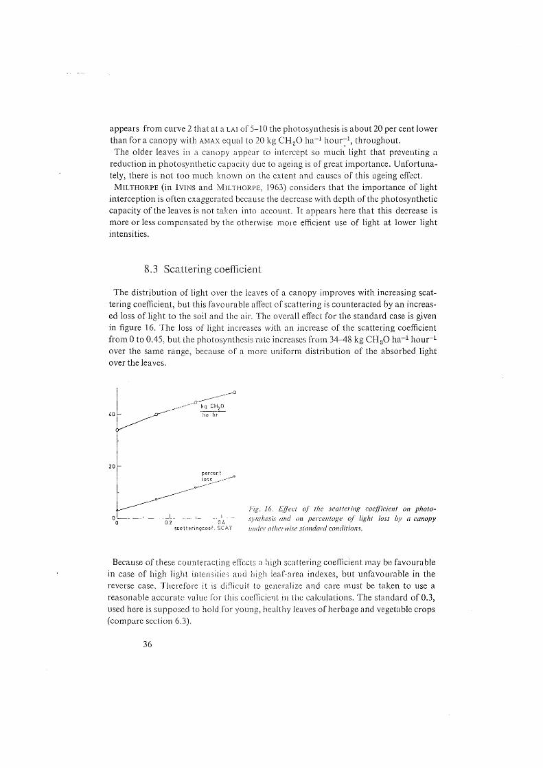
The distribution of light over the leaves of a canopy improves with increasing scat­tering coefficient, but this favourable affect of scattering is counteracted by an increas­ed loss of light to the soil and the air. The overall effect for the standard case is given in figure 16. The loss of light increases with an increase of the scattering coefficient from 0 to 0.45, but the photosynthesis rate increases from 34-48 kg CH20 ha-1 hour-1

over the same range, because of a more uniform distribution of the absorbed light over the leaves.

40

20

0 1--------'------L---'------ __ !_ __

0 02 04 scatteringcoef. SCAT

Fig. 16. Ej}ect of the scattering coefficient on photo­synthesis and on percentage of light lost by a canopy under otherwise standard conditions.

Because of these counteracting effects a high scattering coefficient may be favourable in case of high Jight intensities and high leaf-area indexes, but unfavourable in the reverse case. Therefore it is diff]cult to genera1ize and care must be taken to use a reasonable accurate vJlue for this coefficient in the calculations. The standard of 0.3, used here is supposed to hold for young, healthy leaves of herbage and vegetable crops (compare section 6.3),

36

8.4 Fraction of diffuse light

It is assumed (figure 2 and table 5) that with a clear sky and the sun at 45o, the amount of diffuse light is 16 per cent of the total of0.572 cal cm-2 min-1• The light distribution improves and the photosynthesis rate of the canopy increases of course with an in­creasing percentage of diffuse light at the same total light intensity. The magnitude of this effect is given in figure 17 for the standard case. The effect is large when the both extremes of all direct or all diffuse light are compared, but actually the deviations from the assumed percentage of diffuse light are so small that it is not worthwhile to spend much energy on measuring the fraction of diffuse light in order to improve on the cal­culation of photosynthesis.

40

20

kgC~O

~

I perfectly

clear

0o~----~~--------~so--------~--------_J1oo percent diffuse light

Fig. 17. Effect of the percentage diffuse light on photosynthesis under otherwise standard conditions.

8.5 Inclination of the sun and condition of the sky

The relation between the inclination of the sun and the photosynthesis with a perfect­ly clear sky and with an overcast sky is given in figure 18 for the standard case. The relations between the inclination of the sun and the light intensity in quadrant I are the same as those in figure 2. The photosynthesis rates for the different light intensities are given in quadrant II. At an inclination of 85 degrees, photosynthesis with overcast skies is 55 per cent of

photosynthesis with clear skies, whereas the light intensity is reduced to 20 per cent. The differences in photosynthesis rate are considerably smaller than the differences in light intensity. Tllis is due to the better distribution of diffuse light. For the

37

60 40 kg CH20 ha-1hr"1

o---o clear sky overcast sky

A absorbed light

R ret lee ted

T transmitted ..

cal cm·2 min-1

0.6

0.6

0.4

65

percc!l1t

I

30° 60° 90° IS

Fig. 18. Effect of the inclination of the sun in case of a perfectly clear sky and in case of an overcast sky on photosynthesis of a canopy under otherwise standard conditions. Quadrant I: Relation between the inclination of the sun and light intensity (figure 2). Quadrant Tl: Relation between the fight intensity and photosynthesis rate for the two conditions of the

sky. Quadrant IV: Effect of the inclination of the sun on transmission, reflection and absorption of the

canopy.

38

same reason, photosynthesis at a light intensity of about 0.15 cal cm-2 min-1 is con­siderably higher with overcast skies than with clear skies. The shape of the curves in quadrant II depends of course to a large extent on the leaf distribution function and the photosynthesis function, but the effect of these will be discussed in section 8.8 and 8.6. The amount of light lost by reflection and by transmission is given in quadrant IV.

Although the scattering coefficient is 0.3 and half of the light is scattered upwards, less than 10 per cent of the light is lost by reflection. This is because a part of the light, reflected by lower layers is again absorbed by the upper layers. The reflection and ab­sorption are of course independent of the inclination of the sun with overcast skies. But with clear skies, the reflection of the direct rays decreases with increasing height of the sun, because of the better penetration of the light, whereas for the same reason the transmission increases. The overall effect is such that the absorption varies with about 4 per cent, only.

8.6 Photosynthesis function

The value of E calculated from the standard values of AMAX and HH in table 5 is 357 (kg CH20 ha-1 hour-1) /(cal cm-2 min-1). The photosynthesis rate of leaves with a very high AMAX is of course equal to the absorbed light intensity times this factor. The light lost by transmission and reflection is 11.7 per cent at an inclination of the sun of 45° (figure 18). Since light intensity is 0.572 cal cm-2 min-1 the maximum photosyn-

_ kg c~o ha"1hr"1

E- 357 cal em -2 min -1

60-/

40

10 20 30 40 AMAX

kg CHzO ha-1hr"1

Fig. 19. Effect of the maximum photosynthesis of single leaves (AMAX) on photosynthesis of a canopy under otherwise standard conditions.

39

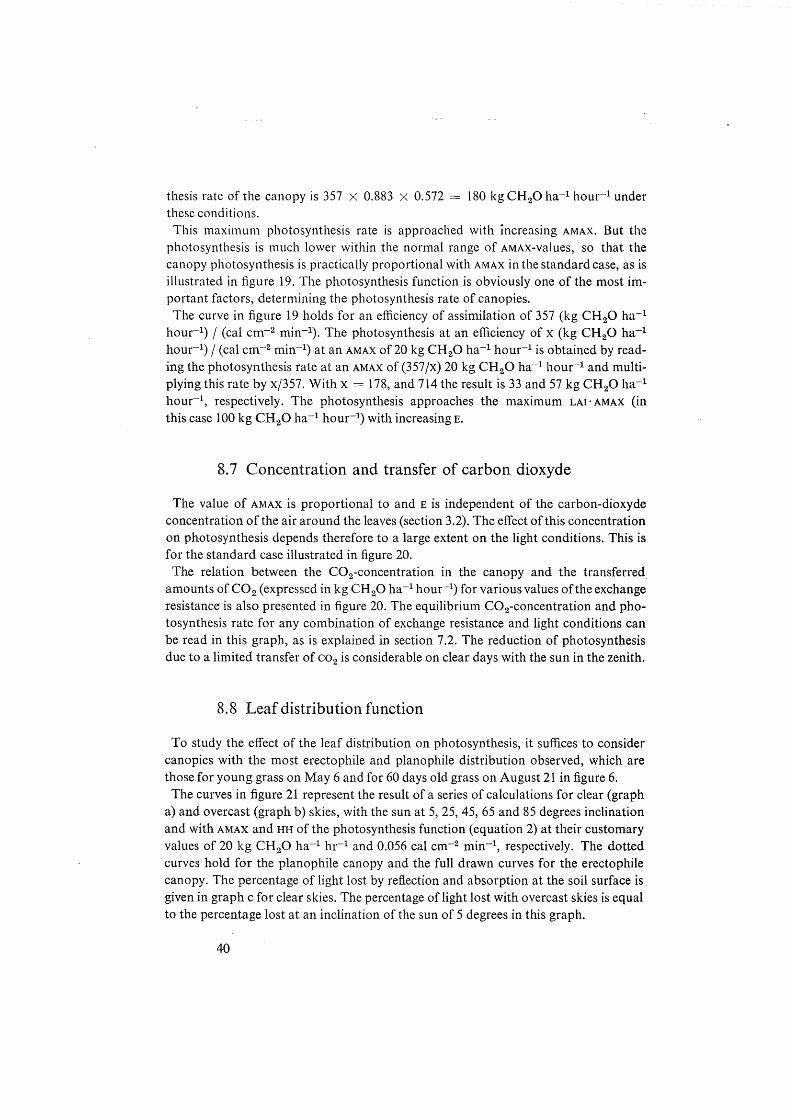
thesis rate of the canopy is 357 X 0.883 X 0.572 = 180 kg CH 20 ha-1 hour-1 under these conditions. This maximum photosynthesis rate is approached with increasing AMAX. But the

photosynthesis is much lower within the normal range of AMAX-values, so that the canopy photosynthesis is practically proportional with AMAX in the standard case, as is illustrated in figure 19. The photosynthesis function is obviously one of the most im­portant factors, determining the photosynthesis rate of canopies. The curve in figure 19 holds for an efficiency of assimilation of 357 (kg CH 20 ha-1

hour-1) / (cal cm-2 min-1). The photosynthesis at an efficiency of x (kg CH20 ha-1

hour-1) /(cal cm-2 min-1) at an AMAX of20 kg CH20 ha-1 hour-1 is obtained by read­ing the photosynthesis rate at an AMAX of (357 fx) 20 kg CH20 ha-1 hour-1 and multi­plying this rate by x/357. With x = 178, and 714 the result is 33 and 57 kg CH20 ha-1

hour-I, respectively. The photosynthesis approaches the maximum LAI· AMAX (in this case 100 kg CH20 ha-1 hour-1) with increasing E.

8. 7 Concentration and transfer of carbon dioxyde

The value of AMAX is proportional to and E is independent of the carbon-dioxyde concentration of the air around the leaves (section 3.2). The effect of this concentration on photosynthesis depends therefore to a large extent on the light conditions. This is for the standard case illustrated in figure 20.

The relation between the C02-concentration in the canopy and the transferred amounts of C02 (expressed in kg CH 20 ha-1 hour-1) for various values of the exchange resistance is also presented in figure 20. The equilibrium C02-concentration and pho­tosynthesis rate for any combination of exchange resistance and light conditions can be read in this graph, as is explained in section 7 .2. The reduction of photosynthesis due to a limited transfer of co2 is considerable on clear days with the sun in the zenith.

8.8 Leaf distribution function

To study the effect of the leaf distribution on photosynthesis, it suffices to consider canopies with the most erectophile and planophile distribution observed, which are those for young grass on May 6 and for 60 days old grass on August 21 in figure 6. The curves in figure 21 represent the result of a series of calculations for clear (graph

a) and overcast (graph b) skies, with the sun at 5, 25, 45, 65 and 85 degrees inclination and with AMAX and HH of the photosynthesis function (equation 2) at their customary values of 20 kg CH20 ha-1 hr-1 and 0.056 cal cm-2 min-I, respectively. The dotted curves hold for the planophile canopy and the full drawn curves for the erectophile canopy. The percentage of light lost by reflection and absorption at the soil surface is given in graph c for clear skies. The percentage of light lost with overcast skies is equal to the percentage lost at an inclination of the sun of 5 degrees in this graph.

40

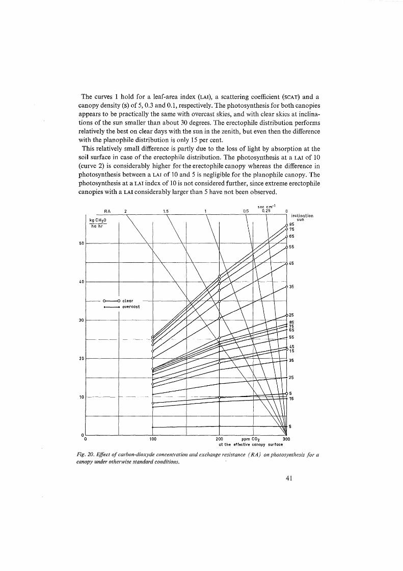
The curves 1 hold for a leaf-area index (LAI), a scattering coefficient (SCAT) and a canopy density (s) of 5, 0.3 and 0.1, respectively. The photosynthesis for both canopies appears to be practically the same with overcast skies, and with clear skies at inclina­tions of the sun smaller than about 30 degrees. The erectophile distribution performs relatively the best on clear days with the sun in the zenith, but even then the difference with the planophile distribution is only 15 per cent. This relatively small difference is partly due to the loss of light by absorption at the

soil surface in case of the erectophile distribution. The photosynthesis at a LAI of 10 (curve 2) is considerably higher for the erectophile canopy whereas the difference in photosynthesis between aLAI of 10 and 5 is negligible for the planophile canopy. The photosynthesis at aLAI index of 10 is not considered further, since extreme erectophile canopies with aLAI considerably larger than 5 have not been observed.

RA

o---o clear ·-overcast

1.5 sec cm·1

0.5 0.25 0 inclination

sun 85 75

65

35

25 30~-------+---------r--~~~T-~~--~~----~-+--~~~~85

75 I s5

~-------+--------~~~~~4-------~~~~~~~-4~~~55

45 .---r:~-'Y15

0~------~--------~--------~------~~------~--------~ 0 100 200 ppm C02 300

at the effective canopy surface

Fig. 20. Effect of carbon-dioxyde concentration and exchange resistance ( RA) on photosynthesis for a canopy under otherwise standard conditions.

41

2

30

4

IS

c 40 t-t

0.51

30

b

overcast

IS

0.1 0.2 cal cm·2min·1

----erectophile , young grass

---- planophile • old gross

curve LA I s SCAT

5 0.1 0.3

2 10 0.1 0.3

3 5 0.3 0.1

4 2 0.1 0.3

AMAX = 20 kg CH20 he-1hr·1 E= 357 (kg CH20 ha-1hr-1)(cal cm·2mln-1)

Fig. 21. Photosynthesis of and percentage of light lost by some canopies under varitJus conditions.

42

The difference between both canopies is also greater when the scattering coefficient is smaller (SCAT = 0.1) and the canopy density is higher (s = 0.3), as illustrated by the curves 3. The less uniform distribution of light makes that the photosynthesis rates of the curves 3 is lower than of the curves 1 over the whole range. The photosynthesis rates at a LAI of 2 are given by the curves 4. The planophile

canopy preforms here better than the erectophile canopy because the disadvantage of a less good light distribution is more than offset by the advantage of a better light interception. The photosynthesis rates for the customary photosynthesis functions and for two

functions with the same efficiency, but an AMAX of 13.3 and 40 kg CH20 ha-1 hr-1 is given in figure 22. The effect of a change in AMAX is considerable, as has been illustrated in section 8.6. But a further discussion of the curves is not necessary, because the rela­tive difference between both distributions is about the same for the three values of AMAX.

erectophile , young gross

---- plonophile . old gross

80 kg CH20 3

40 kg CH20

~ ~

60 30 overcast

2

40 20

20 10

25

OOL-----~----~7-----~-----~1 0.5

col cm·2min·1

LA1=5, SCAT=0.3, 5=0.1, E:357(kg CH20 ha"1hr-1)(col cm"2min"1)

AMAX=13.3, 20ond 40kg CH20 ho"1hr"1for curves 1,2 and 3,resp.

Fig. 22. Photosynthesis of some canopies under various conditions.

45

0.1

3

0.2 col cm"2min" 1

43

9 Daily totals various conditions

It appeared in the previous section that the relative effect of the canopy and leaf characteristics on the photosynthesis may depend to a large extent on the inclination of the sun and the conditions of the sky. Therefore, the relative importance of the effects can only be judged by calculating the overall effect on the course of the daily totals of photosynthesis throughout the year.

This is done for W ageningen (The Netherlands) at a latitude of 51.97 degrees and Kabanyolo (Uganda) at a latitude of 0.47 degrees. Moreover, some tables are given by means of which the daily totals of photosynthesis of a canopy under otherwise stand~rd conditions can be obtained for any place.

9.1 Climate in \Vageningen and Kabanyolo

The daily light totals for Wageningen, assuming that the sky is perfectly clear throughout the year, are presented in figure 23a. The curve for clear days (DE VRIES

1955) gives the light totals on days; when there are no clouds, according to the Camp­bell-Stokes recorder. The difference of about 15 per cent between both curves is due to dust, water vapour and haze. The monthly averages of the daily amount oflight are given by the third curve. These

amounts are obtained by multiplying VAN \VnK's (1963) figures for the total global radiation with 0.5 (section 3. L) Wind speeds at Wageningen given by BRAAK (1943) for a height of 6 meters are con­

verted to a height of 30 meters by multiplying with 1.4. This multiplication factor is obtained by the method outlined in the small print of section 7.2. It is found, that the average wind speed is about 5.7 m sec--1, and that during 10 per cent of the time the wind speed is above 9 m sec--1 and during less than 10 per cent of the time below 2 m sec-1• The corresponding values for RA, found substituting these wind speeds in equation 15, are 0.5, 0.25 and LO sec cm-1, respectively.

The daily light totals in Kabanyolo vvith a perfectly dear sky are given by one of the curves in figure 23b. The other one gives the monthly average of the daily light totals. These amounts were obtained by multiplying the average of HuxLEY's (1961, 1962 and 1963) total global radiation data with 0.5. Wind speeds given by HuxLEY (op. cit.) for a height of 2 meters are converted to 30

meters by multiplication with 2. This multiplic;.'l_tion factor is obtained in the same way as the similar factor for Wageningen. 'The average wind speed is only 2.6 m sec-1,

44

I

cal cm2 day

200

100

a cal cm2 day

200

100

b

KABANYOLO

AMJJASOND JFMAMJ JASOND

Fig. 23. Daily totals of light in Wageningen and Kabanyolo.

whereas the maximum of the daily average wind speed is about 4.8 m sec-1• The values of RA, corresponding with these wind speeds are about 1.0 and 0.5 sec cm-1, respec­tively. The lowest average daily wind speed is about 0.8 m sec-1• The equations (15) and (16) cannot be used to calculate RA at this low wind speed, because mass transfer due to buoyancy of the air cannot be neglected any more (small print of section 7.2). Taking the high temperatures into account it seems reasonable to assume that the maximum value of RA is 1.5 sec cm-1, instead of 3.0, as calculated with equation (15).

9.2 Some widely different canopies

The effect of the height of the sun and the condition of the sky on the photosynthesis rate of the planophile (figure 6, curve 1) and erectophile canopies (figure 6, curve 8) with a leaf-area index of 5, and a canopy density and scattering coefficient of 0.1 and 0.3 or 0.3 and 0.1, respectively has been given in figure 21 for a photosynthesis function with AMAX and E equal to the standard values. These relationships were also calculated for the average RA-values in section 9.1,

and from these the daily totals of photosynthesis in Wageningen and in Kabanyolo were calculated according to the method outlined in section 7.3. These results are presented in figure 24.

45

The effect of the canopy and leaf characteristics on the daily totals of photosynthesis is at most 50 kg CH 20 ha-1 day-1• This difference is relativ~ly small when compared with the daily total of 325 kg CH 20 ha-1 day-1 which was obtained for Wageningert, but on the other hand, a net difference in dry matter production of 50 kg CH20 ha~1

day-1 is high from the agricultural point of view, so that it is better not to pass judge­ment on the importance of the calculated differences at this stage. The daily total of photosynthesis varies in Wageningen from 325 kg CH20 ha-1 day-1 in summer to 60 kg CH 20 ha-1 day-1 in winter. But it must be taken into account that such high photosynthesis rates can only be obtained when the photosynthesis of the leaves is not adversely affected by shortages of water or minerals, by low or high temperatures or by the age of the leaves, and when only a small fraction of dry matter is lost by respira­tion. It has been shown (ALBERDA, 1962, GAASTRA, 1962, MONTEITH, 1962) that actual production rates of canopies may approach these calculated rates.

a

300

200

WAGENINGEN RA= 0.5 sec cm-1

o~~~L-~~~--~~-L~--~~ F M A M J J A S 0 N D

b

100 KABANYOLO RA= 1.0 sec cm-1

Fig. 24. Daily totals of photosynthesis for some canopies in Wageningen and Kabanyolo. The details of the canopies are given in figure 21:

46

9.3 Canopies with spherical leaf distribution

The photosynthesis rate for a canopy at standard conditions at any combination of light condition and exchange resistance can be read in figure 20, and from these the daily totals of photosynthesis can be obtained for any place. The results in Wageningen and Kabanyolo are given in figure 25. The effect of the exchange resistance on the photosynthesis rate is high on clear days

with the sun high in the sky (figure 20), but this condition is even so rare at the equator in Kabanyolo that the overall-effect of wind speed on photosynthesis does not exceed 50 kg CH20 ha-1 day-1. Hence in most cases it suffices to account for the effect of wind speed on photosynthesis by using some average value for the exchange resistance. The daily total of photosynthesis of a canopy under standard conditions and with an

exchange resistance of 0.5 sec cm-1 can be calculated for any arbitrary place and time of the year by means of table 6 and local data on light totals. This table contains for every tenth degree latitude and for the middle of each month

the daily totals of photosynthesis on days with perfectly clear and with overcast skies, and the daily total oflight on a perfectly clear day. The daily total of light on an over­cast day can be obtained from the latter by multiplying with 0.2 (section 3.2). The daily total of photosynthesis is obtained from the actual daily total of light by

linear interpolation.

kg CH20 ha day a kg CH20

ha day

~00

b

___.x--x-x x "'-x x-x-x--x

300 - • ....--•-•-•........._ ""--x-x-x/ -+-+-+ ·-..........._0_./-·-·-·

+ ........... '-+-+-+/+-+-+-+

KABANYOLO

RA (sec/em)

0.50 1.00

+ 1.50

O '--';-~F:--:M:':-~A---:ML-..LJ_JL-..LA----'SL__-LO ---INL-.1-D O J F M A M J J A S 0 N 0

Fig. 25. Daily totals of photosynthesis of a canopy in Wageningen and Kabanyolo with various values of the exchange resistance ( RA) but otherwise under standard conditions.

47

Table 6. The daily totals of light and photosyll/ltesisfor a canopy under standard conditions (tuble 5) and RA = 0.5 sec cm-·1• HC is the light on very clear days and is expressed if} cal cm-·2 day-1 (400-700 11t!.L). The light intensity on overcast days is 0.2 times HC.

PC and PO are the daily totals of photosynthesis on very clear and ow?rcust days, respecth•ely, and e~re expressed in kg CH20 ha-1 day--1•

North 15 15 15 15 15 15 15 15 15 15 15 15 Lat. Jan. Febr. March Apr. May June July Aug. Sept.' Oct. .-.lov. Dec.

HC

PC

PO

HC

PC

PO

HC

PC

PO

HC

PC

PO

HC

PC

PO

HC

PC

PO

HC

PC

PO

HC

PC

PO

HC

PC

PO

HC

PC

PO

48

343 360 413 424 219 226

299 332 376 401 197 212

249 293 334 371 170 193

191 245 281 333 137 168

131 190 218 283

99 137

73 131 147 223 60 100

369 429 230

359 422 225

337 407 215

303 385 200

260 353 178

207 310 150

364 349 337 342 426 417 410 413 228 221 216 218

375 377 374 375 437 440 440 440 234 236 235 236

375 394 400 399 439 460 468 465 235 246 250 249

363 400 417 411 437 471 489 483 232 251 261 258

339 396 422 413 427 480 506 497 223 253 268 263

304 380 418 405 409 484 522 509 207 251 273 265

357 368 365 422 429 427 225 230 2.28

377 369 345 439 431 411 235 230 218

386 357 313 451 425 387 242 226 203

384 333 270 456 412 356 243 216 182

369 298 220 455 390 314 23~ 200 155

344 254 163 448 358 260 230 178 121

22 66 19

72 . 149 260 356 151 254 383 487 60 114 187 245

408 389 309 544 523 .436 276 265 216

201 316 148

103 195 82

0 0 0

20 89 209 331 408 380 269 142 45 65 185 350 506 612 575 427 262 114 16 74 158 241 291 273 200 112 38

0 0 0

0 0 0

0 28 162 334 424 393 248 81 3 0 94 333 571 663 632 474 195 11 0 24 133 257 318 297 196 69 2

0 0 154 339 428 397 252 40 0 0 0 371 588 677 646 497 167 0 0 0 131 269 319 302 215 35 0

349 337 418 410 222 216

311 291 385 370 203 193

264 238 348 325 178 164

210 179 299 269 148 130

151 118 241 204 112 91

92 61 173 130 73 51

37 94 31

2 7

0 0 0

0 0 0

14 49 11

0 0 0

0 0 ·o

0 0 0

When for instance at 60° N.L. on the 5th August, the light intensity is on an average 200 cal cm-2 day-1, the photosynthesis is (F ((113) · 265 + (213) · 216) + (1- F) ((113) · 523 + (213) · 436) kg CH20 ha-l day-1

in which F, the fraction of the time that the sky is clouded, is obtained by working out ((113) · 389 + (213) · 309- 200) 1 (o.s ((113) · 389 + (213) · 309)).

Table 7 contains the daily totals of photosynthesis for the same canopy, but for AMAX being equal to 13.3, 20.0 and 40.0 kg CH20 ha-1 hour-1.

The daily totals for other efficiencies than 357 (kg CH20 ha-1 hr-1) I (cal cm-2 min-1)

can be estimated from these by the interpolation technique described in secti'on 8.6. Estimates of photosynthesis under a large range of conditions can therefore be obtai­

ned by means of the data in table 6 and 7.

Table 7. Daily totals of photosynthesis for a canopy under standard conditions (table 5), but for various values of AMAX.

PC and PO are the daily totals of photosynthesis on very clear and overcast days, respectively, and are expressed in kg CH20 ha-1 day-1 •

20.0 40.0

North 15 15 15 15 15 15 15 15 15 15 15 15 Lat. Dec. Febr. Apr. June Dec. Febr. Apr. June Dec. Febr. Apr. June

0° PC 353 365 367 353 450 467 470 449 649 678 683 649 PO 194 202 203 193 224 234 236 224 269 283 286 269

20° PC 279 319 378 403 350 405 484 516 494 579 704 750 PO 149 173 210 223 170 199 244 259 199 237 295 314

40° PC 176 243 367 435 214 302 467 557 287 418 668 804 PO 86 127 200 240 95 142 230 278 107 164 274 335

60° PC 46 134 329 468 50 158 409 589 57 202 567 833 PO 12 58 171 249 13 63 193 285 13 68 223 336

80° PC 0 0 294 568 0 0 348 703 0 0 446 965 PO 0 0 127 296 0 0 138 330 0 0 151 375

49

10 Fortran programs

THIS SECTION CONTAINS THE FORTRAN PROGRAMS DISCUSSED IN THE SMALL

PRINT OF SECTION 5 AND ]. THEY ARE SMALL ENOUGH TO FIT AN 18M lb2~

COMPUTER WITH 20.000 STORAGE POSITIONS,WHEN WRITTEN WIJH THE NECESSARY

II~PUT CHECKS.

PROGRAM 1

C THE CALCULATION OF THE LIGHT DISTRI8UTION FUNCTION FOR ARBITRARY C VALUES OF THE INCLINATIONS OF THE SUN (IS) AND THE LEAVES (IL). C ARITHMETIC STATEMENT FUNCTION

ARCSF(X)= ATANF(SINF(X)/SQRTF(1-SINF(X)**2)) 22 FORt·1AT(NOT SPECIFIED)

Dlt'IENSION S(19) C 8EGIN STAGE 1

READ 22,1L,IS FIL=IL FIS=IS A=S.N(FIS)*COS(FIL) ~=COS(FIS)*SIN(FIL) PH1=3.1416 X=-A/i3 IF(X+1.)2,2,3

2 DAO=-PH I /2. GO TO 4

3 DAO=ARCSF(X) 4 W=(2.*i3*COS(DA0)-2.*A*DA0)**(-1)

C i3EGIN STAGE 2 DO 5 1=1,19 Fl=l SNLS=-1 ·+Y.i.l *F I SNDA=(SNLS~A)/i3 IF(SNDA+1.)6,6,7

6 S (I )=0. GO TO 5

7 IF(SNDA-1)8,9,9 9 S(l)=1.

GO TO 5 8 DA=ARCSF(SNDA)

IF(DA-DAO) 10,11,11 10 S( l)=(i3~'(COS(DA)-A~'<'(PHI/2.+DA))*W

GO TO 5 11 S(l)=(i3*(2.*COS(DAO)-COS(D4))-A*(2.*DAO+PHI/2.-DA))*W 5 CONTINUE

C 8EGIN STAGE 3 DO 12 1=1,9

1 2 S ( I ) =S ( -1 ~"' I+ 20)-S ( I ) PUNCH 22,(S(I),I=1,9) GO TO 1 END

51

PR0GRAI1 2

C THE CALCULATION OF THE LIGHT DISTRIJUtiON fUNCtiON FOR ARdiTRARY C I NCL I NAT IONS OF THE SUI~ AIW ARt3 I TRARY LEAF' D I STR I t3UT I ON FUNCTIONS. C S(I,J) AftE THE CUI1ULATIVE FREQUEIJCIES OF LIGHT INTERCEPTION AT C SIN(LS) 0-05,~·15, .••••. ~.95 AND AT LEAF INCLINATIONS oF C 5, 15, •••• ,85 DEGHEES.

22 FOR11AT(IWT SPECIFIED) DIMENSION S(9,1~),SN(10),0P(9),F(9),0(1~)

C t3EGIN STAGE 1 READ 22,(( S(I,J),I=1,10),J=1,9) D021=1,10 Fl=l

2 SN ( I ) =-~. )J 5+JJ. 1 ;'rF I DO 3 J=l .9 OP(J)=S(l,J)/SIH1) DO 4 1=2,10

4 OP(J)=OP(J)+(S(J,J)-S(J-1,J))/SN(J) 3 OP(J)=l./OP(J)

C t3EGIN STAGE 2 C F(I,J) AltE THE CUI1ULATIVE FREQUEI~CIES OF THE LEAVES AI LEAr' C INCLIIMTIOIJS OF 5,15, ••••.••• ,&5 DEGREES.

5 READ 22,(F(1),1=1,9) Q=0· DO 6 1=1,9

6 Q=Q+F(J)*OP(J) D071=1,10 0(1)=0. DO 7 J=l 9

7 O(I)=O(I~+F(J)*OP(J)*S(I,J)/Q C 8EGIN STAGE 3

OPG=O(l)/SN(l) DO 8 1=1,10

8 OPG=OPG+(O(J)-0(1-1))/SN(I) OPG=1. /OPG PUtJCH 22, OPG PUNCH 22, (0( I), 1=1, 10) IF(SENSE SWITCH1) 5,1 END

52

t:

PROGRAI-1 3

C THE CALCULATION OF THE PHOTOSYNTHESIS OF A CANOPY FOR ANY C ARBITRARY COMBINATION OF LIGHT,LEAF AND CANOPY CHARATERISTICS. C SN(K) ARE THE SINES OF THE INCLINATIONS OF .?,15, .... ,85 DEGREES, C B(K) ARE THE FRACTIONS OF DIFFUSE LIGHT FROM THESE SKY SECTIONS C AND OP(K) ARE THE PROJECTIONS OF ONE UNIT LEAF SURFACE IN THESE C DIRECTIONS. S AND NI1AX ARE THE CAI~OPY DENSITY AND THE DEPTH OF C THE CANOPY,RESPECTIVELY.

22 FORI"'AT( NOT SPECIFIED) DIMENSION OP(9)~SN(9),B(9),X(9),Y(9),Q(102),P(102),0(10),Z(10) Dlt1ENSION R(102)

C BEGIN ~TAGE 1 READ 22,(0P(K),SN(K),B(K),I=1,9) READ 22, S, Nt1AX DO 2 K=1,9 X(K)=1.-S*OP(K)/SN(K) IF(X(K))3,2,2

3 PUNCH 22,K,X(K) X(K)=0.

2 Y(K)=1. DO 4 1=1,102

4 Q (I )=0. Q(2)=1. DO 5 1=3,Nt-1AX+2 DO 5 K=1,9 Y(K)=Y(K))'cX(K)

5 Q ( I ) =Q ( I ) + Y ( K) )'c t3 ( K) PUNCH 22, (Q( I), 1=1 ,NI1AX+2)

C BEGIN STAGE 2 C SCAT IS THE SCATTERING COEFFICIENT AND FD AND FS ARE THE DIFFUSE C AND DIRECT LIGHT WITH THE SUN AT ONE OF THE INCLINATIONS C (INCL) OF 5,15, ....•.. ,85 DEGREES.

6 READ 22, FD,FS,SCAT,INCL DO 7 1=1,102

7 R (I) =0. K=( INCL+5)/10 QS=1 .-OP(K)*S/SN(K) IF(QS)8,9,9

8 QS=0· 9 El=l.

DO 10 1=2,NMAX+1 E2=E1 ~'<'QS RI=(Q( 1)-Q(I+l))*FD*(1.-SCAT) R(I)=R(I)+RI R I= ( 1J. 51cSCAT I ( 1 .-SCAT) )*R I+ ( E1-E2))'<'FS~'<'0. 5*SCAT DO 11 L= 1 , 1-1

11 R(I-L)=R(I-L)+(Q(L+1)-Q(L+2))*RI R(1)=R(1)+Q(I+1)*RI DO 12 1=1,NMAX-1+2

12 R( I+L)=R( I+L)+(Q(L+l )-Q(L+2) )·kRI R (HAX+2)=R (NI1AX+ 2)+Q ( I~MAX-1+4 )*R I

10 E1=E2 R(NMAX+2)=(R(NMAX+2)+E2*FS+Q(NMAX+2)*FD)*0.9 R I= ( I!J. 1 hL 9) )'cR ( NI1AX+ 2) DO 13 1=2,NMAX+1

1 3 R ( Nt1AX+ 3- I ) =R ( NI1AX+ 3- I ) +R p'c ( Q ( I ) -Q ( I+ 1 ) ) R(1)=R(1)+RI*Q(NMAX+2)

C BEGIN STAGE 3 C AI1AXH AIW HHH.AND AIAAXL AND HHL ARE THE VALUES OF THE CONSTANTS IN C THE PHOTOSYIHHES IS FUI~CT I ON FOR THE HIGHEST AND LOWEST LEAVES IN ~ THE CANOPY. 0(1) ARE THE CUMULATIVE FREQUENCIES OF THE LIGHT C DISTR18UTION FUNCTION FOR SIN(LS) EQUAL TO ~.05,~.15, ...•. ,~.95 C AND THE PROPER INCLINATION OF THE SUN.

14 READ 22, At1AXH,At"'AXL,HHH,HHL READ 22,(0(1),1=1.10)

53

DO 15 L=2 10 15 Z(12-L)=Ot12-L)-0(11-L)

z ( 1 )=0 ( 1 ) E1=1. A=0. DO 16 1=2,NMAX+1 V=( 1-2)/(NMAX-1) HH=HHH-V*(HHH-HHL) AMAX=AMAXH-V~'t(M1AXH-At1AXL) E2=E1 ,'~'QS H=R (I) /S H1=H A1=(H/(H+HH))*AMAX A=A+A 1~'rS IF(FS)16,16,17

17 A=A-Al*(E1-E2)*SN(K)/OP(K) DO 18 L=1,10 FL=L H=(0.05+~·1*FL)*FS*(1 .-SCAT)/SN(K)+Hl

18 A=A+ ( E 1-E 2) trz ( L) *SN ( K) )'c ( H/ ( H+HH)) *AMAX/ (~.II) 5+!0. 1 *F L) 16 El=E2

FT=FS+FD RIF=R(l)/FT RN2F=H(NHAX+2)/FT . PUNCH 22,A,FT ,R(1) ,R(NI1AX+2) ,R1F ,RN2F IF(SENSE SWITCH1) 14,19

19 JF(SENSE SWJTCH2) 6,1 . END

54

~

c c c c

c

c

c c c

PROGRAM 4

THE CALCULATION OF THE DAILY TOTALS OF PHOTOSYNTHESIS FOR ANY ARBITRARY PLACE. D(l) IS THEDECLINATION OF THE SUN ON 5,15,25JAN, .... ,5,15,25DEC. P IS THE LATITUDE OF THE PLACE. FH(K) AND Fd(K) ARE THE LIGHT INTENSITIES AND AH(K) AND A~(K) THE PHOTOSYNTHESIS RATES ON PERFECTLY CLEAR AND OVERCAST DAYS WITH THE SUN AT 5, •.....• ,85 DEGREES.

22 FOR11AT(NOT SPECIFIED) DIMENSION D(36),FH(9),FB(9),AH(9),A8(9),S(10),CH(24),SFH(36) DIMENSION SFB(36),SAH(36),SAB(36) BEGIN STAGE 1 READ 22,(0(1),1=1,36) READ 22,P READ 224(FH(K),FB(K),AH(K),AB(K),K=1,9) PHJ=3.1 16 DO 2 J=2,10 FJ=J

2 S(J)=SINF((5.+10.*(FJ-2.))*PHJ/160.) S(1)=0· CP=COS(P) SP=SINF(P) DO 3 K=1,24 FK=K

3 CH(K)=COSF(0.5+(FK-1.)''cPHI/24.) BEGIN STAGE 2 DO 4 1=1,36 SFH(I)=0. SFB (I) =0. SAH( I )=0 · SAB( I )=0. CD=COSF(D(I)) SD=SINF(D(I)) DO 4 K=1,24 SX=SP*SD+CP*CD*CH(K) IF(SX)Lj.,4,5

5 DO 10 J=2,9 IF(S(J)-SX)6,6,7

6 J~~~X~~~~~?~~/(S(J)-S(J-1)) l SFH(I)=SFH(I)+60.*(FH(J-1)+Q*(FH(J)-FH(J-1)))

SFB(I)=SFB(I)+60.*(FB(J-1)+Q*(FB(J)-FB(J-1))) SAH(I)=SAH(I)+ AH(J-1)+Q*(AH(J)-AH(J-1)) SAB(I)=SAB(I)+ AB(J-1)+Q*(AB(J)-AB(J-1)) GO TO 4

10 CONTINUE 4 CONTINUE

PUNCH 22,(SFH(K),SFB(K),SAH(K),SAB(K),K=1,36) BEGIN STAGE 3 R IS THE DAILY LIGHT TOTAL ON SUCCESIVELY 5,15,25JAN, ••.•••••• ,5,15,25DEC.

8 DO 9 K=1,36 READ 22 R P=SAB(K~+(R-SFB(K))*(SAH(K)-SAB(K))/(SFH(K)-SFB(K)) PUNCH 22,P

9 CONTINUE JF(SENSE SWJTCHl) 1,8 END

55

Literature

ALBERDA, TH.

BERNHARDT, F. and H. PHILLIPS

BOYSEN JENSEN, P. BoYsEN JENSEN, P.

BRAAK, C.

DOGNIAUX, R.

EVANS, L. T. FRITZ, S.

GAASTRA, P.

GAASTRA, P.

GAASTRA, P.

HOPKINSON, J. M.

HEINICKE, H. J. and M. B. HoFFMAN

HUXLEY, P. A.

Iv1Ns, J. D. and F. L. MILTHORPB

JoNES, L. A. and H. R. CoNDIT

KIMBALL, H. H. and I. F. HAND

KLEIN, w. H.

LARCHER, W.

MET. TABLES Moss, D. N.

56

1962

1958

1932 1949

1942

1954

1963 1949

1959

1962

1964

1964

1933

1961-1963

1963

1948

1921

1948

1963

1951 1964

Actual and potential production of agricultural corps. Neth. J. Agric. Sci. 10: 325-333. Die raumliche und zeitliche Verteilung der Einstrahlung und der Strahlungsbilanz im Meeres-Niveau. Teil I. Die Einstrah­lung. Berlin. Die Stoffproduktion der Pflanzen. Jena, 108 pp. The production of matter in agricultural plants and its limi­tation. Bioi. Med. 21: 1-28. Het klimaat van Nederland. D. Wind. Meded. en Verh. KNMI 46: 1-109. Etude des climats de Ia radiation en Beige. Bijdrage KMI, Ukke/ No. 18. Environmental control of plant growth. New York. Solar radiation during cloudless days. Heating and Vent. 46: 69-74. Pl)otosynthesis of crop plants as influenced by light, carbon­dioxyde, temperature and stomatal diffusion resistance. Meded. Landb. Hogesch. Wageningen 59 (13). Photosynthesis of leaves and field crops. Neth. J. Agric. Sci. 10: 311-324. ;, Optimum rates of photosynthesis of field crops. Xth. Bot. Congress, Edinburgh, ab~tr. 004. Studies on the expansion of the leaf surface IV. Exp. Bot. 15: 125-138. The rate of photosynthesis of apple leaves under natural con .. ditions. Cornell Un. Agr. Sta. Bull. 577. Meteorological data for Makerere University College Farm, Kabanyolo, Uganda, 1960, 1961, 1962. Met. Bull. 1-3 (1961-1963). . The growth of the potato. London.

Sunlight and skylight as determinants of ._photographic expo­sure. J. Optical Soc. Amer. 38: 123-178. Sky-brightness and daylight illumination measurements. Monthly Weather Rev. 49:481-487. Calculation of solar radiation and the solar heat load on man. J. of Met. 5: 119-129. Die Leistungsfahigkeit der C02-assimilation hoherer Pflan­zen unter Laboratoriumsbedingungen und am natlirlichen Standort. Mitt.f/or.-soc. Arbeitsgem. N.F. Heft 10:20-34. Smithsonian meteorological tables. Washington, 6th ed. Optimum lighting ofleaves. Crop Science 4: 131-135.

MONSI, M. and T. SAEKI

MONTEITH, J. L.

Moss, R. A. and W. E. LOOMIS

NICHIPOROVICH, A. A.

NICIDPOROVICH, A. A.

PENMAN, H. L.

RABINOWITCH, E. I.

RIDER, N. E.

SAEKI, M.

SEYBOLD, A. and A. WEISSWEILER

TAGAYEVA, S. V. and A. B. BRANDT

TANNER, C. B. and W. L. PELTON

VRIES, D. A.

WIJK, w. R. VAN WIT, c. T. DE

WIT, c. T. DE

1953

1962

1952

1954

1961

1948

1951

1954

1959

1942

1960

1960

1955

1963 1958

1959

Dber den Lichtfaktor in den Pflanzengesellschaften und seine Bedeutung ftir die Stoffproduktion. Jap. J. Bot.14: 22-52. Measurement and interpretation of carbon-dioxyde fluxes in the field. Neth. J.: Agr. Sci.JO: 334-346. Absorption spectra of leaves. I. The visible spectrum. Pl. Physiol. 27: 370-391. Photosynthesis and the theory of obtaining high crop yields. XVth Timiryazev Lecture, Moskou. Properties of plant crops as an optical system. Soviet Pl. Physiol. 8:428-435. Natural evaporation from open water, bare soil, and grass. Proc. roy. Soc. (A), 193: 120-146. Photosynthesis and related processes. Vol. II, Part I, New York. Evaporation from an oat field. Quart. J. R. met. Soc. 80: 198-212. Variation of photosynthetic activity with ageing of leaves and total photosynthesis in a plant community. Bot. Mag., Tokyo 72:404-408. Spektrophotometrische Messungen an grtinen Pflanzen und an Chlorophyll-Losungen. Bot. Arch. 43:252-290. Study of the optical properties of leaves in relation to the angle of incidence of light. Biofizika 5: 308-317. Potential evapotranspiration estimates by the approximate energy balance method of Penman. J. geophys. Res. 65: 3391-3413. Solar radiation at Wageningen. Med. Landb. hogesch. Wage­ningen 55:277-304. Physics of plant environment. Amsterdam. Transpiration and crop yields. Versl. Landbouwk. Onderz. 64.6. Potential photosynthesis of crop surfaces. Neth. J. Agric Sci. 7: 141-149.

57