Photometriccalibrationofwide-fieldskysurveydatafromMini-MegaTORTORA

S.Karpov (FZU AV CR, SAO RAS, KFU) on behalf of Mini-MegaTORTORA team

Mini-MegaTORTORA• Wide-field monitoring system

• 9 channels 10x10 deg each • Sub-second temporal resolution

• 10 fps default, exposures up to 60 s • Multi-regime operation

• 3 color + 1 polarimetric filters • Real-time transient detection, classification

and follow-up• Follow-up of external triggers

Mini-MegaTORTORAskysurveyMini-MegaTORTORA typically monitors every 30x30 deg field for ~1000 seconds

60-s (later 3x20 s) white light frames are acquired before and after monitoring every field

Crowded fields, wide band, bad PSF, coelostat mirrors, …

482000 frames in total760 nightsVlim ~ 13-14 mag

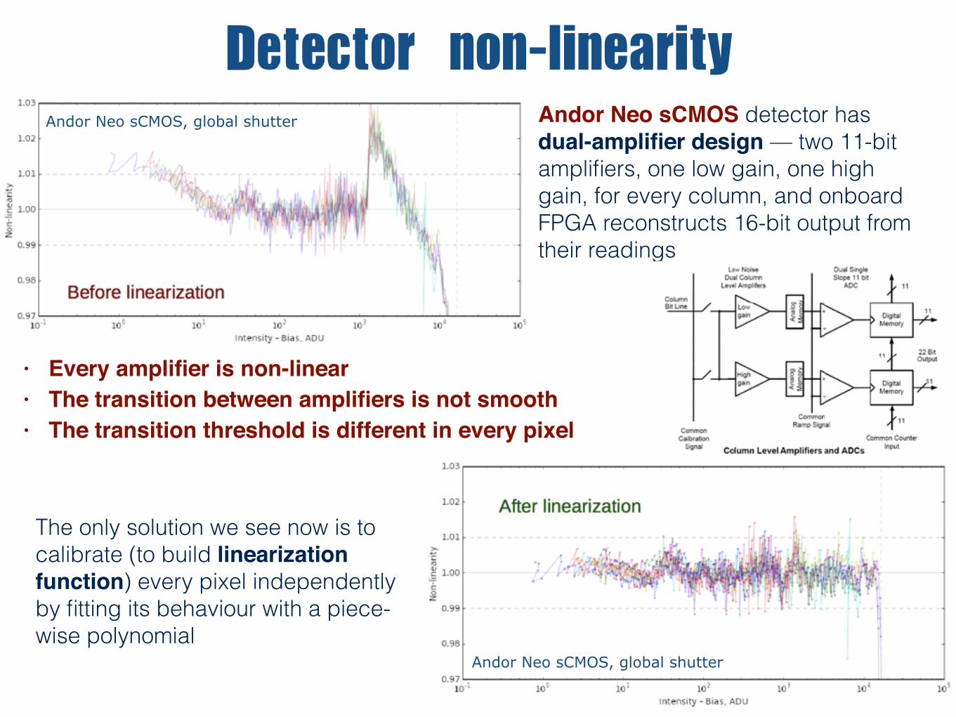
Detectornon-linearity

• Every amplifier is non-linear• The transition between amplifiers is not smooth• The transition threshold is different in every pixel

Andor Neo sCMOS detector has dual-amplifier design — two 11-bit amplifiers, one low gain, one high gain, for every column, and onboard FPGA reconstructs 16-bit output from their readings

The only solution we see now is to calibrate (to build linearization function) every pixel independently by fitting its behaviour with a piece-wise polynomial

Andor Neo sCMOS, global shutter

Andor Neo sCMOS, global shutter

Detectorbiaslevelinstability 0

0.05

0.1

0.15

0.2

90 95 100 105 110 115 120 125no

rmal

ized

occ

urre

nce

count

acceptable pixel | counts histogram | shutter: rolling

baseline

Figure 9: Histogram for series above

70

80

90

100

110

120

0 2000 4000 6000 8000 10000

coun

t

frame #

unsuitable pixel #1 | successive counts history | shutter: global

baseline

Figure 10: History of dark signal in the “bad” pixel #1 with global shutter.

7

0

0.05

0.1

0.15

0.2

40 60 80 100 120 140 160

norm

aliz

ed o

ccur

renc

e

count

unsuitable pixel #2 | counts histogram | shutter: global

baseline

Figure 15: Histogram for series above

96

98

100

102

104

106

0 2000 4000 6000 8000 10000

coun

t

frame #

acceptable pixel | successive counts history | shutter: global

baseline

Figure 16: History of dark signal in the “good” pixel with rolling shutter.

10

40

60

80

100

120

140

160

0 1000 2000 3000 4000 5000 6000 7000 8000 9000 10000

coun

t

frame #

unsuitable pixel #2 | successive counts history | shutter: global

baseline

Figure 13: History of dark signal in the “bad” pixel #2 with global shutter.

50

60

70

80

90

100

110

120

130

140

2500 2600 2700 2800 2900 3000

coun

t

frame #

unsuitable pixel #2 | successive counts history [fragment] | shutter: global

baseline

Figure 14: Fragment of previous curve

9

20

40

60

80

100

120

140

160

4000 4100 4200 4300 4400 4500 4600

coun

t

frame #

unsuitable pixel #1 | successive counts history [fragment] | shutter: rolling

baseline

Figure 11: Fragment of previous curve

0

0.01

0.02

0.03

0.04

0.05

0.06

0.07

0.08

70 80 90 100 110 120

norm

aliz

ed o

ccur

renc

e

count

unsuitable pixel #1 | counts histogram | shutter: global

baseline

Figure 12: Histogram for series above

8

bad pixelbad pixel

bad pixel good pixel

Typicalframes• Dark current is negligible on

typical exposures

• No obvious cosmetic defects

• Biases are being acquired by averaging ~1000 dark frames with 0.1 s exposure

• No way to do proper “evening sky” flats - either too bright or too many stars or clouds

• … plus systematic gradients!

• “photometric superflats”

• “night sky flats” — thresholded median averaging of all acquired survey frames

“Nightskyflats”

Successfully recovers both large-scale (vignetting) and small-scale (amplifier columns, cosmetic defects, …) flatfield variations

• Cluster all images by channels and hardware configurations

• Subtract bias level • Mask stars in every image • Normalize • Median average every ~100 frames • Average the medians

Atypicalframes:-)

Masking• Badly behaving detector pixels

unusable in general

• firmware masked hot pixels • highly non-linear pixels • pixels with “long memory”

• Multi-scale background where background estimation will be biased

• compute background on different meshes, e.g. 32 and 256 pixels

• locate significant deviations • dilate with large kernel

• Large object sizes extended wings

• extract objects, get sizes • threshold • dilate with small kernel

Imagequality

DedicatedPSFphotometrycode

• Linearization, simple masking and normalization

• Background estimation using Bijaoui (1980) like estimator

• PSF reconstruction using PSFEx

• Optimal filtering with PSF for peak detection

• Simultaneous fitting of peaks in sub-regions

• De-blending in sub-regions

Available at https://github.com/karpov-sv/extract

results are too noisy

Simpleaperturephotometry

• Linearization, complex masking and normalization

• pip install sep

• “Naive” sigma-clipping background estimation

• SExtractor-like object detection

• Adaptive masking of image artefacts

• multi-scale background filtering

• thresholding on object size

• dilution of masks around outliers

• Simple circular aperture photometry

• Fixed aperture or FWHM-based

• No de-blending!

Photometriccalibration

All survey frames are acquired in white light with (time-dependent) system

instrumental = mag0 + V + CBV(B-V) + CVR(V-R) + …

• (Position dependent) mag0, CBV, CVR may be reconstructed using large number of catalogue stars in the frame • Tycho2 with ~60 stars per square degree, BT + VT or conversion to B + V

• Pickles (2010) — template-based recalibration to synthetic mags in all bands!

• APASS DR9 with ~380 stars per sq.deg, B + V + g + r + i

• We may get true V either by • using catalogue B-V and V-R • repeating the observations under different atmospheric conditions and then

fitting for B-V and V-R by minimizing V scatter

• …or just select a close comparison star with the same colors

Single-framecalibration• Local Astrometry.Net for WCS

• sub-pixel accuracy in 10x10 deg!

• Pickles (2010): Tycho2 + 2MASS + NOMAD

• original BT, VT, J, H, K + synthetic magnitudes

• Filtering of “blended” stars

• Count fainter 2MASS stars around every Tycho2 star

• Model with color + 4th order spatial term

• Instr = V + Z0 + CBV (BT-VT)

pixel size

Individual Common, bandpass + secondary extinction

Colorterm

no color term linear color term

cloudy clear

Multi-framecalibration

• Collect all measurements in a given field

• different frames, different channels, different conditions, …

• Cluster points within some radius

• spherical -> 3d Cartesian -> KD tree

• Regress for colors

• Filter frames with lots of outliers

• Repeat using mean values and colors as a reference catalogue

Mean magnitudes are consistent with input catalogue

Derived colors are also mostly consistentthe poor man’s SYSREM

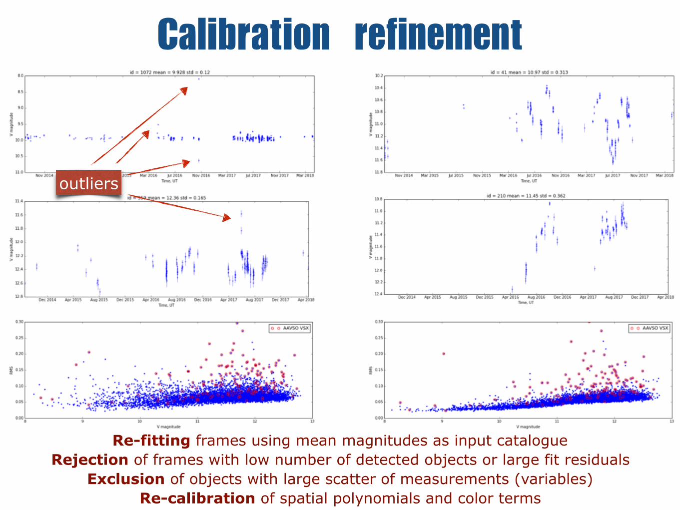
Calibrationrefinement

outliers

Re-fitting frames using mean magnitudes as input catalogue Rejection of frames with low number of detected objects or large fit residuals

Exclusion of objects with large scatter of measurements (variables) Re-calibration of spatial polynomials and color terms

VariabilityPeriod search using code fromhttps://www.astroml.org/gatspy/

W Vir

W UMasemi-reg

Mira

AAVSO

Uncataloguedvariables

TYC4360-1264-1

Detectionproblems

Photometricaccuracy

0.02 mag min RMS

• Detector non-linearity

• Atmospheric conditions

• Analysis artefacts

• Aperture noise?

• Fixed-pattern noise?

...ENDdedicated calibration run of 1000x10 s consecutive frames on a fixed sky field

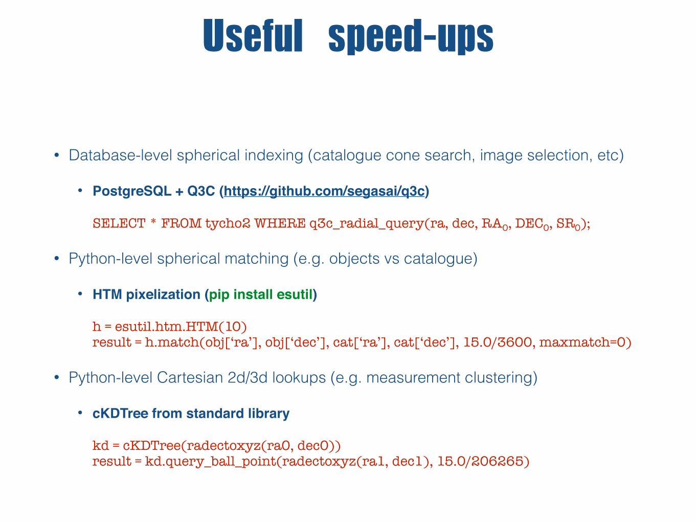
Usefulspeed-ups

• Database-level spherical indexing (catalogue cone search, image selection, etc)

• PostgreSQL + Q3C (https://github.com/segasai/q3c) SELECT * FROM tycho2 WHERE q3c_radial_query(ra, dec, RA0, DEC0, SR0);

• Python-level spherical matching (e.g. objects vs catalogue)

• HTM pixelization (pip install esutil) h = esutil.htm.HTM(10)result = h.match(obj[‘ra’], obj[‘dec’], cat[‘ra’], cat[‘dec’], 15.0/3600, maxmatch=0)

• Python-level Cartesian 2d/3d lookups (e.g. measurement clustering)

• cKDTree from standard librarykd = cKDTree(radectoxyz(ra0, dec0)) result = kd.query_ball_point(radectoxyz(ra1, dec1), 15.0/206265)