Photoionized plasma analysis Jelle Kaastra. Introduction.
68
Photoionized plasma analysis Jelle Kaastra
-
Upload
barnard-lindsey -
Category
Documents
-
view
224 -
download
0
Transcript of Photoionized plasma analysis Jelle Kaastra. Introduction.

Photoionized plasma analysis
Jelle Kaastra

Introduction

What is a photoionised plasma?
• Plasma where apart from interaction with particles also interaction with photons occurs
• Photon spectrum needs to affect the particles (e.g. heating)
• Thus, plasma with resonant scattering has photons involved but is not photoionised (although resonance scattering also occurs in photoionised plasmas)

It is all about the optical depth
• Optical depth τ = 0: collisional• Optical depth τ ≠ 0 but not τ >> 1: classical
photoionised plasma• Optical depth τ >>1: more atmosphere-like or
stellar interior-like, not discussed here• Note: optical depth depends on photon
energy – the above is rather crude

Examples of photoionised plasmas
• Accreting sources:– Galactic X-ray binaries– Active galactic nuclei
• Tenuous gas (like some components of the ISM/IGM)
• Nova shells

Feeding the monster
• Gas transported from 1020 to 1012 m scale
• Disk forms due to viscosity / B-fields / loss angular momentum
• Only few Msun/year reach black hole
6

Outflows from the monster
• Not all gas reaches black hole• Outflows through magnetised jets, disk winds,
outflows from torus surrounding disk• Gives feedback to surroundings, but how much?
7

Basics

9

10

11
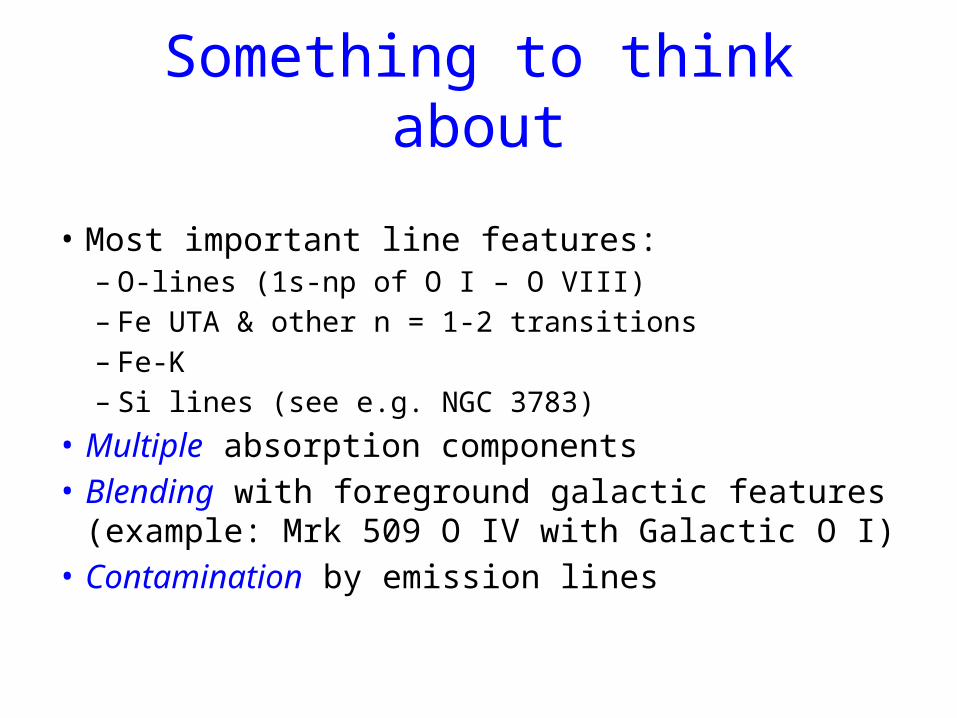
Something to think about
• Most important line features: – O-lines (1s-np of O I – O VIII)– Fe UTA & other n = 1-2 transitions– Fe-K– Si lines (see e.g. NGC 3783)
• Multiple absorption components• Blending with foreground galactic features (example:
Mrk 509 O IV with Galactic O I) • Contamination by emission lines
Photoionisation equilibrium

Key parameter: ionisation parameter
• Spectrum depends on ratio photons / particles• Common used (Xstar, SPEX): ξ = L / nr2 with:
– L = ionising luminosity between 1 – 1000 Ryd (13.6 eV – 13.6 keV; note the upper boundary!)
– n is hydrogen density (NB, different from ne!)– r is distance from ionising source
• Alternative (Cloudy): UH = QH / 4πcnr2 with:– QH number of H-ionising photons (13.6 Ryd – ∞)
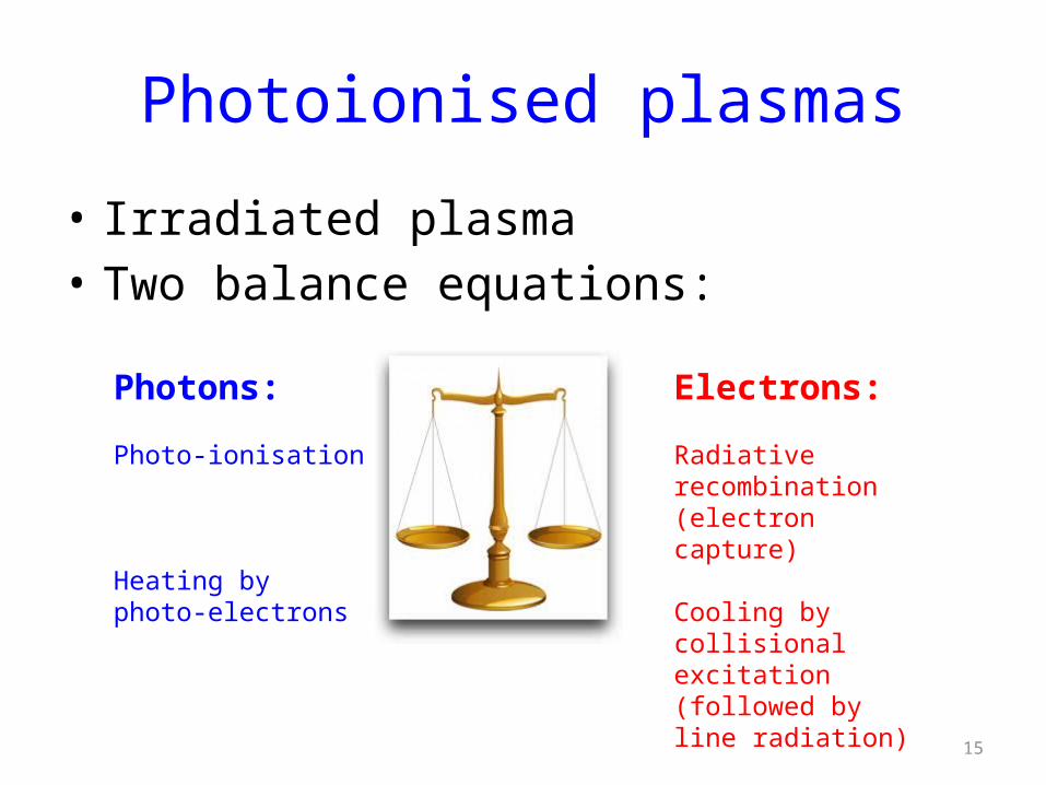
Photoionised plasmas
• Irradiated plasma• Two balance equations:
15
Photons:
Photo-ionisation
Heating by photo-electrons
Electrons:
Radiative recombination (electron capture)
Cooling by collisional excitation (followed by line radiation)
16
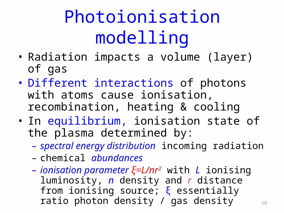
Photoionisation modelling
• Radiation impacts a volume (layer) of gas• Different interactions of photons with atoms
cause ionisation, recombination, heating & cooling
• In equilibrium, ionisation state of the plasma determined by:– spectral energy distribution incoming radiation– chemical abundances– ionisation parameter ξ=L/nr2 with L ionising luminosity,
n density and r distance from ionising source; ξ essentially ratio photon density / gas density

First balance equation: ionisation stages (1)
• Same rates as for CIE plasmas:• Collisional ionisation• Excitation auto-ionisation• Radiative recombination• Dielectronic recombination• At low T, charge transfer ionisation &
recombination

First balance equation: ionisation stages (2)
• New for PIE plasmas:• Photoionisation• Compton ionisation (Compton scattering of
photons on bound electrons; for sufficient large energy transfer this leads to ionisation)

Second balance equation: energy
• Balance: heating = cooling• Take care how heating etc is defined: we use
here heating/cooling of the free electrons• For instance, for e-+ione-+ion++e- we assign
the ionisation energy I to the cooling of the free electrons

Heating processes
• Compton scattering (photon looses energy)• Free-free absorption• Photo-electrons• Compton ionisation• Auger electrons• Collisional de-excitation

Cooling processes
• Inverse Compton scattering (photon gains energy)
• Electron ionisation• Recombination• Free-free emission (Bremsstrahlung)• Collisional excitation
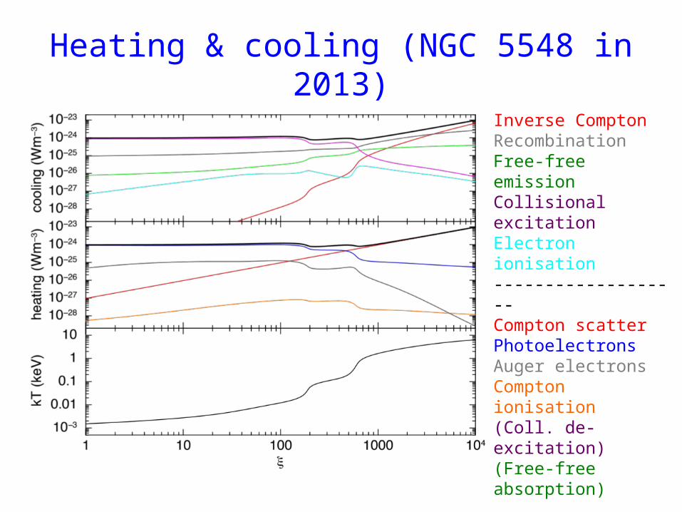
Heating & cooling (NGC 5548 in 2013)Inverse ComptonRecombinationFree-free emissionCollisional excitationElectron ionisation-------------------Compton scatterPhotoelectronsAuger electronsCompton ionisation(Coll. de-excitation)(Free-free absorption)

Heating & cooling (NGC 5548 obscured)Inverse ComptonRecombinationFree-free emissionCollisional excitationElectron ionisation-------------------Compton scatterPhotoelectronsAuger electronsCompton ionisation(Coll. de-excitation)(Free-free absorption)
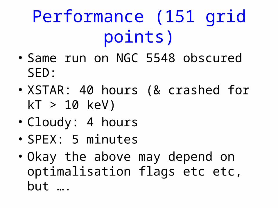
Performance (151 grid points)
• Same run on NGC 5548 obscured SED:• XSTAR: 40 hours (& crashed for kT > 10 keV)• Cloudy: 4 hours• SPEX: 5 minutes• Okay the above may depend on optimalisation
flags etc etc, but ….

Performance
• Often people make a grid of models as function of few parameters table grid feed into favorite fitting program
• SPEX pion model allows fast instantaneous calculation & simultaneous fitting of the continuum of any shape; multiple stacked layers

Stability photo-ionisation equilibrium(examples from Detmers et al. 2011)
• Ξ = Fion/nkTc = ξ/4πckT
• Stable equilibrium for dT/d Ξ > 0
26

Stability curves differhere case NGC 5548 (Mehdipour et al. 2014)

Other useful representations (same data as previous slide)

Differences photo-ionisation models (Mrk 509 SED)
29

Differences photoionisation models(NGC 5548 obscured case)

Photoionisation modelling
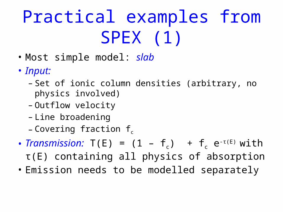
Practical examples from SPEX (1)
• Most simple model: slab• Input:
– Set of ionic column densities (arbitrary, no physics involved)
– Outflow velocity– Line broadening– Covering fraction fc
• Transmission: T(E) = (1 – fc) + fc e-τ(E) with τ(E) containing all physics of absorption
• Emission needs to be modelled separately

Practical examples from SPEX (2)
• next simple model: xabs• Input:
– Set of ionic column densities pre-calculated using real photoionisation code
– Ionisation parameter ξ = L/nr^2– Outflow velocity– Line broadening– Covering fraction fc
• Transmission: T(E) = (1 – fc) + fc e-τ(E) with τ(E) containing all physics of absorption
• Emission needs to be modelled separately

Practical examples from SPEX (3)
• next simple model: warm• Input:
– Set of ionic column densities pre-calculated using real photoionisation code
– Absorption measure distribution dNH(ξ)/dξ, parametrized by powerlaw segments
– Outflow velocity– Line broadening– Covering fraction fc
• Transmission: T(E) = (1 – fc) + fc e-τ(E) with τ(E) containing all physics of absorption
• Emission needs to be modelled separately
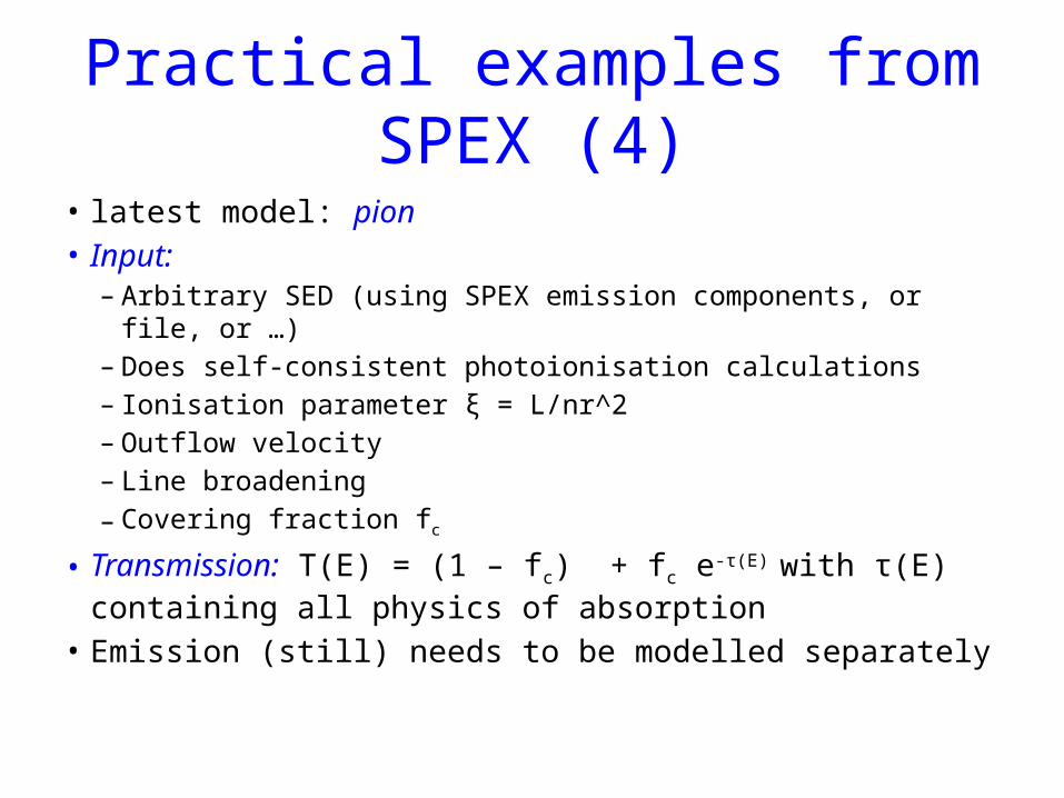
Practical examples from SPEX (4)
• latest model: pion• Input:
– Arbitrary SED (using SPEX emission components, or file, or …)– Does self-consistent photoionisation calculations– Ionisation parameter ξ = L/nr^2– Outflow velocity– Line broadening– Covering fraction fc
• Transmission: T(E) = (1 – fc) + fc e-τ(E) with τ(E) containing all physics of absorption
• Emission (still) needs to be modelled separately

Future extensions of the pion model
• Include also emission (using SPEX plasma code core; several processes need updates)
• Cooling at low T not yet accurate enough (Rolf Mewe’s CIE model stopped at K-like ions or higher)
• Thicker layers (simple radiation transport using escape factors)
• NB only the Titan code takes full radiative transfer into account

Absorption measure distribution (AMD)

Absorption Measure Distribution
38
Ionisation parameter ξ
Em
issi
on m
easu
re
Col
umn
dens
ity Discrete components
Continuousdistribution
Temperature

39
Decomposition into separate ξ
• Early example: NGC 5548
(Steenbrugge et al. 2003)• Use column densities Fe
ions from RGS data
• Measured Nion as sum of separate ξ components
• Need at least 5 components

40
Separate components in pressure equilibrium, or continuous?
Discrete components in pressure equilibrium?
Continuous NH(ξ) distribution?
Steenbrugge et al. 2005
Krongold et al. 2003

Discrete ionisation components in Mrk 509?Detmers et al. 2011 paper III
• Fitting RGS spectrum with 5 discrete absorber components (A-E)
• Gives excellent fit
41

42
Continuous AMD model?Mrk 509, Detmers et al. 2011
• Fit columns with continuous (spline) model
• C & D discrete components!
• FWHM <35% & <80%• B (& A) too poor statistics
to prove if continuous• E harder determined:
correlation ξ & NH
• Discrete components
C
D
B
E

Pressure equilibrium? No!
43

A comparison between sources
• All Seyfert 1s show similar trend
• NH increases with ξ like power law
• High ξ cut-off?• Same behaviour in
Seyfert 2s (NGC 1068, Brinkman et al. 2002)

Time-dependent photoionisation

Why study time-dependent photoionisation?
• Because most photoionised sources are time-variable
• Gives opportunity to determine distance of gas from ionising source mass loss, kinetic luminosity etc

“The” recombination time scale
• Pure recombination equilibrium:0 = dni/dt = niRi-1 + ni+1Ri
• This leads, with Ri = neαi to characteristic time
trec = 1 / [ne (ni+1/ni – αi-1/αi)]
• Thus, we see that trec~1/ne
• However, there is always a point where ni(ξ) and ni+1(ξ) are such that trec∞, and this point is usually close to where ni(ξ) peaks!
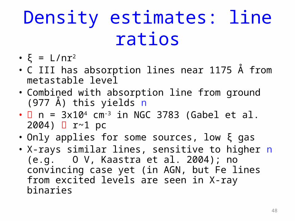
Density estimates: line ratios
• ξ = L/nr2
• C III has absorption lines near 1175 Å from metastable level
• Combined with absorption line from ground (977 Å) this yields n
• n = 3x104 cm-3 in NGC 3783 (Gabel et al. 2004) r~1 pc
• Only applies for some sources, low ξ gas• X-rays similar lines, sensitive to higher n (e.g. O V,
Kaastra et al. 2004); no convincing case yet (in AGN, but Fe lines from excited levels are seen in X-ray binaries
48

49
Density estimates: reverberation
• If L increases for gas at fixed n and r, then ξ=L/nr² increases
• change in ionisation balance • column density changes • transmission changes• Gas has finite ionisation/recombination
time tr (density dependent as ~1/n)• measuring delayed response yields
trnr

Lightcurve Mrk 509 during 100 days(Kaastra et al. 2011, paper I)
50
Soft X-ray
UV
Hard X-ray
• Factor ~2 increase in soft X-ray
• Correlated with UV• No correlation with
hard X-ray

Spectral energy distribution(Mehdipour et al. 2011, paper IV)
51
Soft excess
Power law
DBB

Time-dependent SEDs Mrk 509(Kaastra et al. 2012, paper VIII)
52

Predicted signal
53
Simplified case: predicted change transmission for instantaneous 0.1 dex increase L, at spectral resolution EPIC/pn Signal is weak (1% level) but detectable

Time-dependent calculation
54
Hard X
Soft X
Total
Time evolution ion concentrations ni:dni/dt = Aij(t) nj
Aij(t) contains t-dependent ionisation & recombination rates
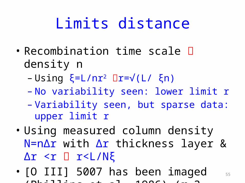
Limits distance
• Recombination time scale density n– Using ξ=L/nr2 r=√(L/ ξn)– No variability seen: lower limit r– Variability seen, but sparse data: upper limit r
• Using measured column density N=nΔr with Δr thickness layer & Δr <r r<L/Nξ
• [O III] 5007 has been imaged (Phillips et al. 1986) (r=3 kpc)
55

Summary distance limit methods for 5 components in Mrk 509
Component MethodLower limit
MethodUpper limit
A Direct imaging [O III] Direct imaging [O III]
B (UV)
C pn & RGS, Fe blend Δr/r<1
D RGS O VIII Long-term pn
E pn, Fe blend Δr/r<1
56

Results: where is the outflow?(Kaastra et al. 2012, paper VIII)
57

Abundances outflow(Steenbrugge et al. 2011, paper VII)
• Relative metal abundances close to Solar
• Absolute abundances await new COS data with hydrogen Lyman series
• Only doable after carefull photoionisation modelling
58

Challenge: NGC 5548 in an obscured state

Surprise: very low soft X-ray flux

Strong absorption but normal high-E flux

Appearance of lowly ionised gas

UV broad absorption lines
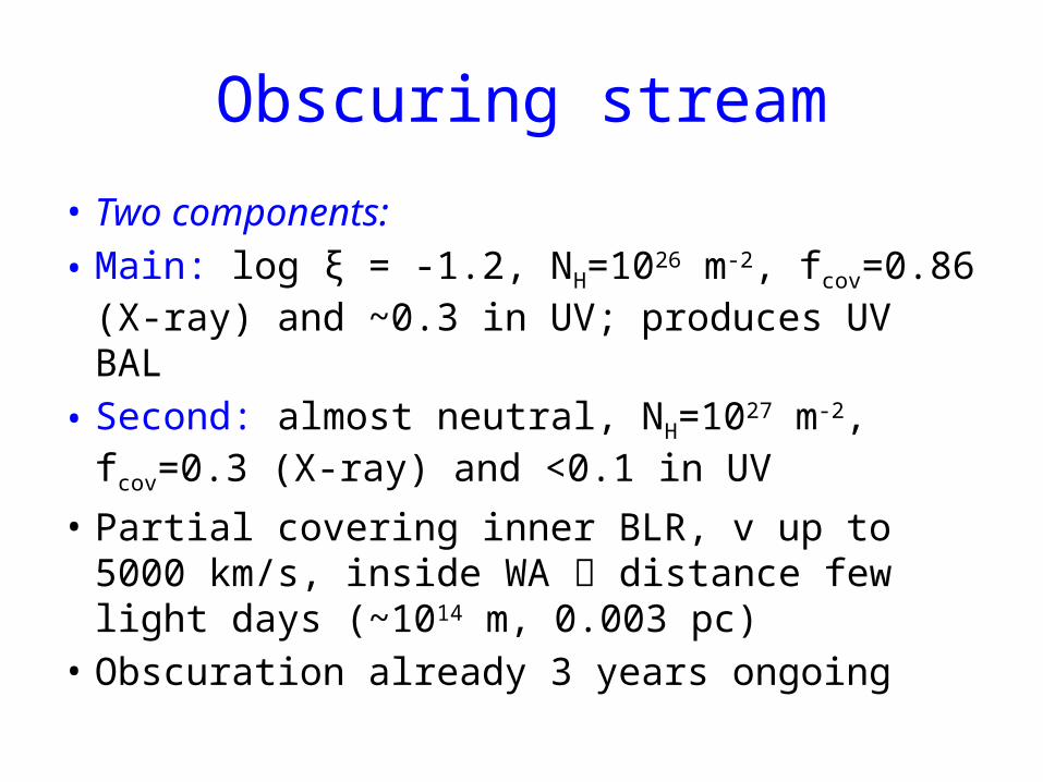
Obscuring stream
• Two components:• Main: log ξ = -1.2, NH=1026 m-2, fcov=0.86 (X-ray)
and ~0.3 in UV; produces UV BAL• Second: almost neutral, NH=1027 m-2, fcov=0.3 (X-
ray) and <0.1 in UV• Partial covering inner BLR, v up to 5000 km/s,
inside WA distance few light days (~1014 m, 0.003 pc)
• Obscuration already 3 years ongoing

What is going on?

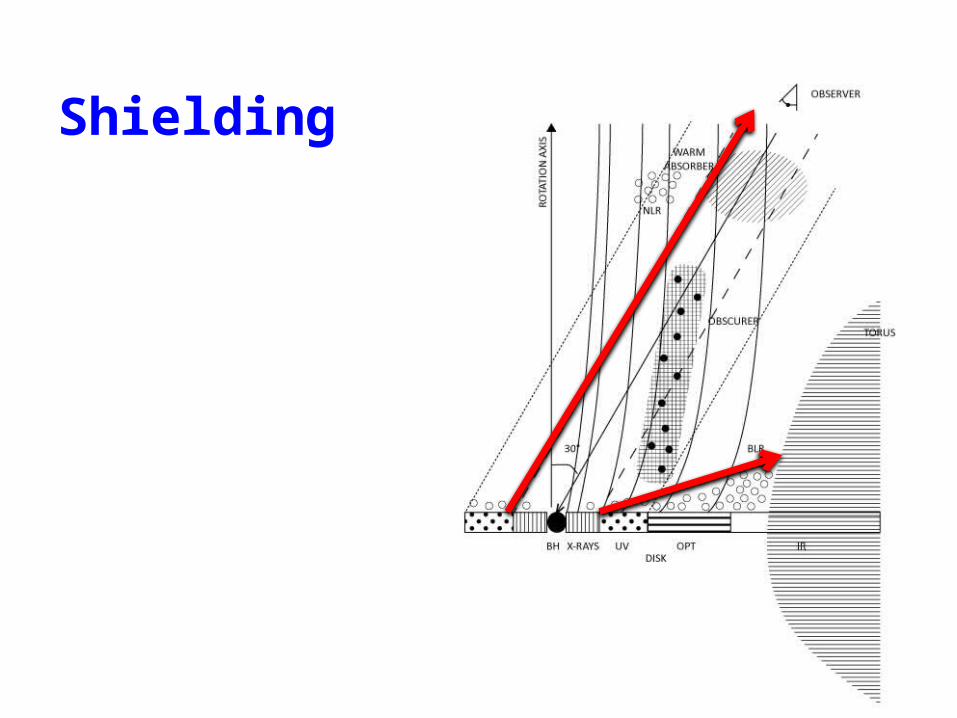
Shielding

Importance for feedback(Murray et al. 1995)