Phenomenological Combustion Modeling for Optimization of ...
170
CZECH TECHNICAL UNIVERSITY IN PRAGUE FACULTY OF MECHANICAL ENGINEERING DEPARTMENT OF AUTOMOTIVE, COMBUSTION ENGINE AND RAILWAY ENGINEERING DOCTORAL THESIS Phenomenological Combustion Modeling for Optimization of Large 2-stroke Marine Engines under both Diesel and Dual Fuel Operating Conditions Ing. Filip Černík Doctoral Study Program: Mechanical Engineering Field of Study: Machines and Equipment for Transportation Supervisor: prof. Ing. Jan Macek, DrSc. Doctoral thesis for the academic degree of ”Doctor“, abbreviated to "Ph.D." Prague February 2018
Transcript of Phenomenological Combustion Modeling for Optimization of ...

CZECH TECHNICAL UNIVERSITY IN PRAGUE
FACULTY OF MECHANICAL ENGINEERING
DEPARTMENT OF AUTOMOTIVE, COMBUSTION ENGINE AND RAILWAY ENGINEERING
DOCTORAL THESIS
Phenomenological Combustion Modeling for Optimization of Large 2-stroke
Marine Engines under both Diesel and Dual Fuel Operating Conditions
Ing. Filip Černík
Doctoral Study Program: Mechanical Engineering
Field of Study: Machines and Equipment for Transportation
Supervisor: prof. Ing. Jan Macek, DrSc.
Doctoral thesis for the academic degree of ”Doctor“, abbreviated to "Ph.D."
Prague February 2018


1
Abstract
A phenomenological simulation methodology for combustion modeling of both liquid and gaseous fuels for
large low speed 2-stroke marine engines is developed and validated within the present study. The work
incorporates modeling concepts for diesel and dual fuel combustion aiming for a physics based and generic
model structure. Phenomenological aspects of these concepts are theoretically investigated and considered
individually in respect of specifics of large uniflow scavenged 2-stroke engines. Individual aspects of fuel
introduction, mixing, ignition and oxidation are taken into consideration with respect to multiple peripheral
injectors, uniflow scavenging with imposed swirl or direct low-pressure gas admission. Implementation of
the resulting models into a commercial 1D simulation tool in form of a user routine allows fast cycle
simulation of full scale engine models or integrated marine power systems at a good level of fidelity. Hence,
the proposed method enables the computationally effective optimization of complex propulsion systems
under both steady and transient operating conditions.
The quasi-dimensional model proposed for diesel combustion is capable of accurate predictions in terms of
heat release rate and engine performance figures based on an imposed injection profile. The model takes
into account the specific design features of the combustion space in large two-stroke engines such as
multiple decentralized fuel injectors or intake air swirl. One of the most important characteristics considered
by the model is the methodology for capturing interactions among individual sprays and an appropriate
adjustment of the locally effective air excess ratio, as the available oxygen is predominant for combustion
progress. If the spray is enclosed by the burned gases of sprays from a neighboring injector, the burn rate
is restricted and later recovered in case suitable conditions are restored. In order to reproduce this behavior,
spatial resolution of the combustion chamber is considered and transformed into a quasi-dimensional and
solely mathematical description. The final burn rate is then determined by a time scale model employing a
simplified zero-dimensional turbulence model considering a typical integral length scale. The availability of
fuel ready to be oxidized is constrained by evaporation, mixing and spray interactions. Extensive validation
is performed against data from experimental investigations in a spray combustion chamber (SCC) and full-
scale engine data. The computation is executed by means of an integrated combustion subroutine using a
dynamic link library interface with the 1D engine model. Instantaneous import of in-cylinder conditions and
injection rates enables immediate prediction of heat release rate. The validity of the model predictions under
various operating conditions is confirmed for several Wärtsilä low-speed marine engine types.
The dual fuel phenomenological combustion model accounts for both diffusion combustion of the liquid pilot
fuel and the flame front propagation through the gaseous premixed charge. In the context of the pilot fuel
model a common integral formulation defines the ignition delay whereas a time scale approach is
incorporated for the combustion progress calculation. In order to capture spatial differences given by the
scavenging process and the admission of the gaseous fuel, the cylinder volume is discretized into a number
of zones. The laws of conservation are applied to calculate the thermodynamic conditions and the fuel
concentration distribution. Subsequently, the ignition delay of the gaseous fuel-air mixture is determined by
the use of tabulated kinetics and the ensuing oxidation is described by a flame velocity correlation.
Computational concepts for both laminar and turbulent flame velocities are determined based on conditions
characteristic for large 2-stroke marine engine operation. Comprehensive theoretical studies and
computational assessments have been accomplished to derive appropriate correlations for propagation of
both laminar and turbulent flames. The resulting heat release rates and pressure traces are validated
against experimental engine data. Sensitivity studies of major parameters related to combustion such as
scavenging temperature, equivalence ratio, pilot timing or compression ratio are performed. Performance
predictions are tested for several engine types and show good level of agreement with measurements.

2
The proposed methodology generalizes phenomenological aspects of combustion in large low speed 2-
stroke marine engines with focus on diesel and dual fuel combustion under both steady and transient
operation conditions. The modeling approach has proved to be viable for the optimization of present and
future marine propulsion systems. Apart from the application to a standalone engine model also an entire
propulsion system with integration of hydraulic models for fuel injection or exhaust valve actuation has been
modeled. The user routine based model structure allows performing standalone or system integrated
calculations and thus facilitates direct utilization for engine optimization. Furthermore, options for model
extension in terms of emission modeling are outlined. The fundamental scientific contribution of the present
work relies on the generation of a better understanding of the complexity of combustion processes in large
low speed 2-stroke marine engines, the identification of the governing phenomena and the derivation of
suitable modelling approaches for reducing the complexity to a level allowing the fast but yet generic
simulation of large 2-stroke engine combustion.

3
Anotace
Disertační práce popisuje vývoj a validaci fenomenologické metodiky simulace spalování kapalných a
plynných paliv ve velkých pomalobežných dvoutaktních lodních motorech. Práce zahrunuje kocept simulace
dieselového a duálního neboli dvoupalivového hoření z cílem vypracování fyzikálně zobecněného modelu.
Fenomenologické aspekty těchto konceptů jsou teoreticky vyhodnoceny z hlediska specifik pomaloběžných
dvoutaktních motorů se souproudým vyplachováním. Začlenění modelu do 1D simulačního softwaru GT-
Suite formou uživateského programu umožňuje časově nenáročné výpočty oběhu pro samostatný model
motoru nebo celkových integrovaných lodních pohoných systémů s požadovanou přesností. Tímto je
umožněna efektivní optimalizace lodních pohonů při stacionárním a transientních podmínkách.
Kvazidimenzionální model navržen pro dieselové spalování umožňuje predikaci průběhu hoření a
výkonových parametrů motoru na základě průběhu vstřiku paliva. Model zohledňuje koncepci spalovacího
prostoru velkého dvoutaktního motoru s několika decentralizovanými vstřikovači a vířivým vyplachovním.
Zásadní součástí dieselového modelu jsou interacke jednotlivých paprsků vstřiku ovlivňující lokální přebytek
vzduchu, který je určující pro průběh spalování. V případě vzájemného překrytí paprsku vstřiku a spalin je
průběh hoření zpomalen. K zotavení hoření nastává když je obnoven dostatečný přebytek vzduchu na
základě rodílu rychlostí paprsku vstřiku a spalin. Pro dosažní těchto požadavků modelu je spalovací prostor
popsán kvazidimenzionálně, což umožňuje řešení průniku a interakce jednotlivých parpsků vstřiku. Celkový
průběh hoření je určen pomocí časového měřítka hoření s využitím bezrozměrného modelu turbulence a
jejího integrálního měřítka. Palivo dostupné pro hoření je definované průběhem vypařování, míšení a
interakcemi parpsků vstřiku. Model dieselového spalování je kalibrován s využitím experimentálních dat
naměřených ve spalovací komoře (SCC) a na motoru. Samotný výpočet probíhá formou integrace
uživatelského programu do 1D modelu motoru, která umožňuje okamžitou výměnu potřebných paremetrů
pro rychlou predicaci průběhu hoření. Validita výsledků metodiky dieselového spalování je ověřena pro
několik typů pomaloběžných dvoutaktních motorů Wärtsilä.
Fenomenologický model duálního spalování v sobě zahrnuje jak model difuzního hoření pilotního vstřiku
tak model pro homogenní hoření zemního plynu. Průtah vznětu pilotního paliva je určen integrální metodou,
zatímco průběh hoření je definován jeho časovým měřítkem. Za účelem modelování prostorových rozdílů
způsobených procesem vyplachovní a přívodem plynného paliva je objem válce diskretizován do několika
zón. Základní zákony zachování jsou využity pro výpočet přestupů hmoty mezi jednotlivými zónami a určení
zónových koncentrací. Průtah vznětu plynného paliva je následně určen pomocí tabelované kinetiky.
Následné hoření homogenní směsi plynu se vzduchem je popsáno rovnicí rychlosti plamene pro podmínky
charakteristické pro velké dvoupalivové dvoutaktní lodní motory. Rychlost šíření plamene je popsána pro
laminární a turbulentní podmínky. Analogicky vzhledem k dieselovému modelu je odvozen bezrozměrný
model turbulence. Výsledné průběhy hoření jsou porovnány s experimentálními daty. Studie citlivosti
výsledků modelu zahrunuje variace základních parametrů jako jsou například přebytek vzduchu, počátek
pilotního vstřiku nebo kompresní poměr. Obecnost a prediktivita model duálního spalování je ověřena pro
různé dvoutaktní lodní motory vzhledem k výsledkům měření.
Navržená metodika zobecňuje fenomenologické aspekty spalování ve velkých pomaloběžných
dvoutaktních lodních motorů se zaměřením na dieselové a duální spalování při stacionárních a transientních
provozních podmínkách. Využití navrženého simulačního přístupu pro optimalizaci bylo oveřeno pro
modelování samostatného motoru i celkových pohonných systémů s integrací hydraulických modelů
vstřikovače a výfukového ventilu. Definice uživatelského programu usnadnňuje přímé využití v 1D
simulačním prostředí včetně možnosti výpočtu emisí. Vědecký přínos této práce spočívá v komplexním
zmapování a zobecnění spalování v pomaloběných dvoutaktních lodních motorech. Charakteristické
aspekty těchto motorů týkající se vstřiku paliva, přípravy směsi a hoření jsou zohledněny z hlediska

4
decetralizovaných vstřikovačů paliva, souproudého vyplachování válce se swirlem nebo přímého
nízkotlakého přívodu plynu do válce.

5
Content
Abstract ........................................................................................................................................................ 1
Anotace ......................................................................................................................................................... 3
Content ......................................................................................................................................................... 5
Nomenclature ............................................................................................................................................... 7
1. Introduction ............................................................................................................................................ 10
2. State of the Art ....................................................................................................................................... 14
2.1 DI Diesel Combustion Modeling ............................................................................................................ 14
2.1.1 Empirical Models ................................................................................................................................ 16
2.1.2 Phenomenological Models ................................................................................................................. 19
2.1.3 Multi-zonal models .............................................................................................................................. 24
2.1.4 Multi-dimensional Models ................................................................................................................... 30
2.2 Dual Fuel Combustion Modeling ........................................................................................................... 31
3. Motivation and Objectives .................................................................................................................... 36
4. Theory ..................................................................................................................................................... 38
4.1 Thermodynamics ................................................................................................................................... 38
4.2 Turbulence ............................................................................................................................................. 39
4.3 Diesel Combustion ................................................................................................................................ 44
4.3.1 Spray Morphology .............................................................................................................................. 45
4.3.2 Evaporation ........................................................................................................................................ 50
4.3.3 Ignition ................................................................................................................................................ 51
4.4 Dual Fuel Combustion ........................................................................................................................... 53
4.4.1 Laminar Premixed Flames.................................................................................................................. 55
4.4.2 Turbulent Premixed Flame ................................................................................................................. 62
4.4.3 Lean Gas Combustion ........................................................................................................................ 69
4.5 Emissions Formation ............................................................................................................................. 71
4.5.1 Nitrogen Oxides .................................................................................................................................. 71
4.5.2 Soot .................................................................................................................................................... 72
5. Diesel Model Formulation ..................................................................................................................... 74
5.1 Modeling Approach ................................................................................................................................ 74
5.2 Spray Model .......................................................................................................................................... 74
5.2.1 Spray Tip Penetration ......................................................................................................................... 75
5.2.2 Spray Dispersion ................................................................................................................................ 77
5.3 Spray Interactions .................................................................................................................................. 78
5.4 Ignition Delay and Premixed Combustion Models ................................................................................ 86
5.5 Diesel Turbulence model ....................................................................................................................... 87
5.6 Diffusion Combustion Model.................................................................................................................. 90
6. Dual Fuel Model Formulation ............................................................................................................... 92
6.1 Modeling Approach ................................................................................................................................ 92
6.2 Pilot Fuel Combustion ........................................................................................................................... 94
6.3 Ignition Delay, Cylinder Discretization ................................................................................................... 99
6.4 Laminar flame speed ........................................................................................................................... 103
6
6.5 Dual Fuel Turbulence Model ............................................................................................................... 106
6.6 Turbulent flame velocity ....................................................................................................................... 108
6.7 Dual Fuel Combustion ......................................................................................................................... 110
7. Results .................................................................................................................................................. 113
7.1 Diesel Model Results ........................................................................................................................... 113
7.1.1 Experimental Setup and Data Acquisition ........................................................................................ 113
7.1.2 Engine Load Variation ...................................................................................................................... 113
7.1.3 Fuel Rail-Pressure Variation............................................................................................................. 116
7.1.4 Injector Nozzle Execution Variation .................................................................................................. 117
7.1.5 Sequential Injection Impact .............................................................................................................. 118
7.1.6 Engine Type and Bore Size .............................................................................................................. 119
7.1.7 Diesel Model Performance Assessment .......................................................................................... 121
7.2 Dual Fuel Model Results ..................................................................................................................... 123
7.2.1 Experimental Setup and Data Acquisition ........................................................................................ 123
7.2.2 Engine Load Variation ...................................................................................................................... 124
7.2.3 Equivalence Ratio Variation ............................................................................................................. 126
7.2.4 Scavenge Air Temperature Impact ................................................................................................... 127
7.2.5 Pilot Injection Timing Variation ......................................................................................................... 129
7.2.6 Engine Speed Variation .................................................................................................................... 129
7.2.7 Compression Ratio Impact ............................................................................................................... 130
7.2.8 Engine Bore Size .............................................................................................................................. 132
7.2.9 Dual Fuel Model Performance Assessment ..................................................................................... 136
7.3 Model Applications .............................................................................................................................. 138
7.3.1 Integrated System Simulation .......................................................................................................... 138
7.3.2 Transient Loading ............................................................................................................................. 142
8. Conclusions ......................................................................................................................................... 147
Acknowledgments ................................................................................................................................... 150
References ............................................................................................................................................... 151
Appendix .................................................................................................................................................. 157
A1 Figures and Tables .............................................................................................................................. 157
A2 NO Formation ....................................................................................................................................... 160
A3 Heat Transfer Model ............................................................................................................................ 161

7
Nomenclature
NOTATION
A [m2] area
a [m2 s-1] thermal diffusivity
B [m] cylinder bore diameter
BM Spalding mass transfer number
cp [J kg-1 K-1] isobaric specific heat
C model constant
D [m2 s-1] mass / molecular diffusivity
Da Damköhler number
d [m] diameter
f function
h [J kg-1] specific enthalpy
Hu [J kg-1] calorific value of fuel
H [J kg-1] latent heat
k [m2 s-2] turbulent kinetic energy
k+ [m3 mol-1 s-1] forward rate constant
k- [m3 mol-1 s-1] reverse rate constant
K [s-1] Karlovitz flame stretch factor
Ka Karlovitz number
lI [m] integral length scale
L [J kg-1] latent heat of vaporization
LM [m] Markstein length
Le Lewis number
M [kg mol-1] molar mass
Ma Markstein number
m [kg] mass
Nu Nusselt number
Oh Ohnesorge number
p [Pa] pressure
Pr Prandtl number
r [m] radius
R [J K-1 mol-1] gas constant
Re Reynolds number
SL [m s-1] laminar flame speed
ST [m s-1] turbulent flame speed
Sh Sherwood number
s [m] spray penetration
t [s] time
T [K] temperature
u [m s-1] velocity
u’ [m s-1] turbulence intensity
V [m3] volume
w flux sign coefficient
We Weber number
xb burn rate
Y mass concentration
Ze Zeldovich number

8
[s-1] flame stretch
[°] horizontal spray angle
[m] flame thickness
[m2 s-3] dissipation rate
[m] Kolmogorov microscale
ratio of specific heat
[W m-1 K-1] thermal conductivity
[N s m-2] dynamic viscosity
[m2 s-1] kinematic viscosity
[kg m-3] density
mathematical constant
s] characteristic time
equivalence ratio
°CA] crank angle
SUBSCRIPTS
ad adiabatic
b burned
conv convection
diff diffusion
dr droplet
eff effective
exh exhaust conditions
f fuel
fo formation
fl flame
G Gibbson
g gas
I integral
IP inlet ports
i index
in intake conditions
ini initial
L laminar
l liquid
n number of zones
noz nozzle
rad radiation
ref reference state
res residuals
s soot
scav scavenging
st stoichiometric
ox oxidation
pist piston
prem premixed
T turbulent
tan tangential
u unburned

9
ACRONYMS
0D zero-dimensional
1D one-dimensional
3D three-dimensional
CA crank angle
CMCR contract maximum continuous rating
CFD computational fluid dynamics
CR compression ratio
DATDC degree after top dead center
DF dual fuel
EOI end of injection
EVC exhaust valve close
EWG exhaust waste gate
FAST fuel actuated sacless injectors
GAV gas admission valve
GAVO gas admission valve open
HFO heavy fuel oil
HRR heat release rate
IMO International Maritime Organization
IPO Inlet port open
LFO light fuel oil
MEP mean effective pressure
MFB mass fraction burned
MN methane number
PCC pilot combustion chamber
PDF probability density function
PIT pilot injection timing
RPM revolutions per minute
SMD Sauter mean diameter
SOC start of combustion
SOI start of injection
SR substitution rate
TC turbocharger
VCU valve control unit

10
1. Introduction
The combustion process in reciprocating engines as a mean of conversion of chemical energy of the primary
fuel compounds into thermal energy and ultimately into mechanical work has become fundamental in major
means of transportation, industry and agriculture. Moreover, the role of reciprocating engines in the power
generation segment which turns to be even more inherent considering the rising prevalence of renewable
energy sources.
Essentially, combustion process is an overall exothermic reaction where fuel and oxidizer are being
consumed. Except for the heat generation undesirable products are formed. Those are in majority
environmentally harmful, e.g. nitric oxides or carbon dioxide. Improving the thermal efficiency of the
combustion process and minimizing its negative effects represent a decisive aspect of the numerous
research efforts over past decades. Moreover, due to the energy market volatility, dwindling supply and in
reaction on tightening emission regulations optimization of present propulsion systems and development of
novel concepts is inevitable. Additionally, the power and propulsion solutions have to be sophisticated
enough to aim for competitive capital and operational expenditures regardless of the complexity required.
In this respect, the present study aims at computational methodology allowing fast and predictive
computational simulation for development and optimization of such concepts.
Since the first diesel engine was patented in 1892, it has become well established energy convertor across
the entire industry in numerous applications. Moreover, the importance of diesel engine has increased
together with tightening the environmental regulations thanks to its high thermal efficiency related to
increased compression ratios and its throttle-less operation. Nevertheless, due to unburned hydrocarbons
and particulate matter high priority has to be given to pollutant reduction for future acceptance of a diesel
engine. Despite of the often discussed harmful effects of particulate matter in context with urban mobility
and comparably higher NOx production, DI diesel engines possess a potential for low emission level through
aftertreatment additionally enhanced by introducing various strategies such as 2-stage turbocharging, EGR
or extreme Miller timing. Especially in the marine market of large container, bunker or tanker vessels a low
speed two-stroke diesel engine represents often the only reasonable propulsion alternative due to direct
propeller drive or capability to burn HFO fuels. Although emissions pollutions in marine segment is closely
linked to the fuel quality and cannot be neglected, shipping remains to be the most effective mean of
transportation demonstrated visually in Figure 1.
Figure 1 Means of transport ranking by CO2 emissions discharge
11
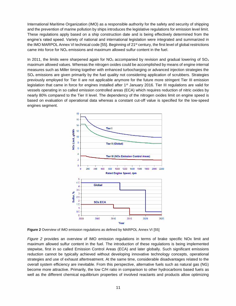
International Maritime Organization (IMO) as a responsible authority for the safety and security of shipping
and the prevention of marine pollution by ships introduces the legislative regulations for emission level limit.
These regulations apply based on a ship construction date and is being effectively determined from the
engine’s rated speed. Variety of national and international legislation were integrated and summarized in
the IMO MARPOL Annex VI technical code [55]. Beginning of 21st century, the first level of global restrictions
came into force for NOx emissions and maximum allowed sulfur content in the fuel.
In 2011, the limits were sharpened again for NOx accompanied by revision and gradual lowering of SOx
maximum allowed values. Whereas the nitrogen oxides could be accomplished by means of engine internal
measures such as Miller timing together with enhanced turbocharging or advanced injection strategies the
SOx emissions are given primarily by the fuel quality not considering application of scrubbers. Strategies
previously employed for Tier II are not applicable anymore for the future more stringent Tier III emission
legislation that came in force for engines installed after 1st January 2016. Tier III regulations are valid for
vessels operating in so called emission controlled areas (ECA) which requires reduction of nitric oxides by
nearly 80% compared to the Tier II level. The dependency of the nitrogen oxides limit on engine speed is
based on evaluation of operational data whereas a constant cut-off value is specified for the low-speed
engines segment.
Figure 2 Overview of IMO emission regulations as defined by MARPOL Annex VI [55]
Figure 2 provides an overview of IMO emission regulations in terms of brake specific NOx limit and
maximum allowed sulfur content in the fuel. The introduction of these regulations is being implemented
stepwise, first in so called Emission Control Areas (ECA) and later globally. Such significant emissions
reduction cannot be typically achieved without developing innovative technology concepts, operational
strategies and use of exhaust aftertreatment. At the same time, considerable disadvantages related to the
overall system efficiency are inevitable. From this perspective, alternative fuels such as natural gas (NG)
become more attractive. Primarily, the low C/H ratio in comparison to other hydrocarbons based fuels as
well as the different chemical equilibrium properties of involved reactants and products allow optimizing

12
carbon dioxide emissions and improvement of thermal efficiency, respectively. Independently on the primary
energy source, the main challenge for developing future marine propulsion systems consists in overcoming
the conflicting objectives for efficiency improvement while fulfilling emissions regulations.
In this regard, the optimization of diesel combustion process and associated emissions formation will remain
of major importance together with an inevitable introduction of exhaust aftertreatment solutions. Aiming for
comprehensive optimization of the combustion process all substantial physical phenomena taking place
during fuel injection spray penetration and breakup, evaporation, mixture formation, ignition and oxidation
need to be considered. Moreover, the chemical processes linked to preflame reactions, thermal cracking,
oxidation and thermal energy liberation cannot be neglected. They play an essential role especially in terms
of ignition delay determination and emissions formation. With respect to diesel engine, the key strategy to
attain high efficiency, complete combustion and moderate emissions production are linked to the spray
characteristics that have a crucial impact on the turbulent mixing process and the subsequent burning
progress. Especially in case of large 2-stroke marine engines, the swirling in-cylinder flow field together with
multiple circumferential located injectors increase the complexity. Despite numerous past research projects
on fundamentals listed above, these have not been sufficiently explored and mapped on the field of low
speed 2-stroke engine. Therefore, the application of generic and fast computational models for engine
development and optimization is rather limited due to the lack of validation data. Nevertheless, this has
change within past years due to extensive research efforts accomplished in Spray Combustion Chamber
(SCC) [45,127,128]. The SCC test rig in a size of a full scale 2-stroke engine combustion space allows
executing basic research activities both related to spray morphology and combustion process. Implementing
findings of the experimental work into mathematical models in becomes essential for definition of a rigorous
and generic combustion modeling approach. Utilization of such predictive models integrated into cycle
simulation tools already at the early stage of the development process can reduced total development costs
substantially in case of large marine engines.
Figure 3 Comparison of relative emissions lever for a diesel and DF engine in gas mode [91]
Recently, as the use of natural gas for power generation and transportation dramatically expands it is also
becoming increasingly attractive for both landlocked and transoceanic shipping. Flexible engine operation
on both liquid and gaseous fuels is often desirable in marine applications, for example due to safety issues.
In this respect, the dual fuel (DF) technology well proven in Wärtsilä 4-stroke DF engines offers the required

13
fuel flexibility while maintaining high efficiency and reliability [121]. One of the main advantages of the lean
burn concept is the ability to fulfill the IMO Tier III emissions regulation without any need of exhaust gas
aftertreatment. Figure 3 compares significant potential to reduce emissions compared to a reference diesel
case as demonstrated on Figure 20.
With respect to a large low speed 2-stroke engine, features such as turbocharger with exhaust waste gate
(EWG) control, common rail injection and variable exhaust valve drive facilitate the conversion from a diesel
to dual fuel engine operation. The DF concept combines benefits from operation on HFO and NG and thus
stands for an attractive propulsion alternative in terms of fuel selection when operating inside of ECAs or for
LNG tanker applications. Although there have been several attempts in the past, the industrialization of a
large marine 2-stroke DF engine has failed mainly due to technical issues and moderate emissions limits.
Recently, the situation has changed dramatically and current studies have confirmed the feasibility of such
a concept with all its benefits by numerous experimental validations on multi-cylinder test and production
engines [91,96]. However, many fundamental questions related to the implementation of the lean burn
combustion concept in large marine 2-stroke engines remain unresolved since the technology maturation
has not been achieved yet. Therefore, computational studies can provide valuable information with respect
to the detailed processes and specific requirements for dual fuel combustion with low-pressure gas
admission in large 2-stroke engines. The ability to carry out effective design changes, define engine
performance and extend the lean burn concept to other engine bore sizes including the feasibility for various
fuel qualities require detailed understanding of the processes taking place before and during combustion.
Computational modeling has been recognized as a useful tool to support the engine design and
performance development. Furthermore, it can also be utilized for effective analysis of experimental results.
Especially in case of low-pressure DF combustion it is of high importance to capture properly individual
phenomena linked to pilot diesel injection, evaporation and subsequent diffusive combustion interacting with
the gas-oxidizer charge that results into the turbulent premixed flame propagation. It is also worth noting
that the stochastic character of the premixed combustion with its sensitivity to the mixture homogeneity and
instabilities due to gas composition variations and stratification has to be assessed carefully. Improper
selection of engine settings may lead to potential incidence of knock or misfiring cycles. Describing the
complexity of DF combustion in large 2-stroke marine engines, physical based modeling approach is
required generic validity. Three-dimensional, transient and highly turbulent character of the mixing,
evaporation and oxidation processes are being well captured by a detailed CFD simulation. Nevertheless,
these models are time consuming and do not allow multi-parameter engine cycle simulation studies of entire
propulsion systems under both steady and transient operation conditions. Aiming for fast and generic
modeling approach phenomenological models need to be developed and validated.
Stringent emissions limits, rising focus on operational costs and market volatility increase the demand on
effective, environmental and flexible propulsion systems for commercial shipping sector. Generic and fast
running engine models help to accelerate and facilitate the development of propulsions concepts addressing
these requirements. The following state of the art summarizes past modeling efforts for both diesel and dual
fuel combustion modes. Subsequently, a predictive combustion modeling approach is developed with
respect to phenomenological aspects of a large uniflow scavenged 2-stroke marine engines. Although there
have been many attempts until now to develop physical, predictive and computationally efficient combustion
models according to the author’s best knowledge no suitable models for large 2-stroke marine engines
applications are have been developed so far that would cover both diesel a dual fuel concept accordingly.
Following the state of the art study in Section 2 motivation and thesis goals are outlined. Introduction of
related theory in Section 4 leads to model formulation of diesel and DF combustion modes with the focus
on the phenomenological interpretation of spray interactions and ignition process, respectively. In the
Section 7, model validation and results of the developed models integrated into a 1D cycle simulation tool
are presented. Finally, several case studies for marine engine applications under steady state and transient
conditions are presented to demonstrate the model feasibility for development and optimization of present
and future propulsion systems.

14
2. State of the Art
2.1 DI Diesel Combustion Modeling
As already outlined in the introduction, the tightening environmental regulations and customer requirements
force engine manufacturers to strive for new and innovative ways of improving the engine performance and
reduce emissions at the same time. Hence, new combustion strategies are needed to fulfil often
contradictory requirements for high efficiency and low NOx and soot emissions. Figure 4 provides an
overview of some of these diesel combustion strategies where CI stands for the common compression
ignition diffusion combustion in engines with direct injection. Alternative concepts introduce a shift from
conventional approach towards new types of combustion regimes commonly denoted as low temperature
combustion (LTC) showing promising results in terms of significant emission reduction. Just to mention a
few, homogenous charge compression ignition (HCCI) or premixed charge compression ignition (PCCI) with
favorable trade-offs between high degree of thermal efficiency and moderate emission levels make these
concepts attractive. However, applications are often constrained to a limited load range.
Figure 4 Diesel combustion regimes classification on – T map according to [90]
For both conventional and alternative combustion concepts, numerical modeling is becoming more
important already within the concept development phase. Over past decades, computational modeling of
internal combustion engines has become essential for engine developers for a wide spectrum of
applications. Use of simulation models may improve the process of engine development substantially when
straining for optimum fuel economy and low emissions at the same time. In this respect, deeper
understanding of individual processes implemented in a predictive and reliable simulation tools is necessary
in order to mature innovative, economically viable and ecological solutions. In this way, multiple parameter
simulation studies can be carried out and thus testing cost are reduced considerably. In this regard, the
modeling of engine combustion phenomena counts for a core expertise within the engine development
process. Such trend penetrates throughout the whole range of engine product categories including large
slow speed 2-stroke engines. Employing purely empirical concepts for heat release calculation persists to
be essential and partly remains favorable as well. However, such concepts are often based on past engine
types with limited output and obsolete technology. On the other hand, present engines are designed for high
power densities with extensive firing pressure and high level of parameter flexibility due to advanced control
strategies. In this context, phenomenological modeling approach is preferable for its general validity while
relying on the physical interpretation of fuel injection, evaporation, mixing and oxidation. For even better

15
accuracy discretization of the combustion space in two or more zones is appropriate and allows tracking of
temperature and composition for emissions formation prediction. Multi-dimensional model offers much more
complex solution on elementary level by spatial resolved thermodynamic condition and distribution of
individual species. Nevertheless, referring to the objectives outlined in the previous section due to a
significant computational demand multi-dimensional approach in terms of CFD modeling has not been
considered within the scope of this work.
Combustion models can be classified in three main categories according to their complexity directly
proportional to computational time requirement; zero-dimensional, quasi-dimensional and multi-
dimensional. An overview on the classification of combustion model is presented in Figure 5 summarizing
the main features and capabilities of the individual categories.
Figure 5 Classification of combustion models with respect to physical fidelity and computational effort
Zero-dimensional simulations abstract real processes in order to focus on the outcome without exploring
the actual background. These concepts and predominantly outlined as single-zone models represent an
empirical combustion approximation by a simple mathematical function or a combination of several
functions. This formula links indirectly combustion with several parameters which are being adjusted in order
to fit the measured heat release preferably over a whole operation range and if possible also for various
engines. It should to be noted that those parameters do not have necessarily any physical meaning and are
deliberately calibrated merely by measured data. In cylinder thermodynamic conditions are averaged, no
interaction with injection spray evolution is being considered at all. Such models are typically
computationally very fast and are suitable for application without any requirements on combustion
predictivity outside the calibration region, e.g. gas exchange simulations or various parameter optimization
studies. In case of a single zone approach composition and temperature uniformity is being assumed.
Theoretically, in case of implementing 2-zonal approach emission formation could be also calculated.
However, as a matter of averaged conditions within the zones and therefore due to the lack of spatial
temperature and composition resolutions such estimations result in rather poor conformity with
measurements.
Quasi-dimensional models stand for an intermediate step between zero- and multi-dimensional concepts
combining some of their features and advantages. These phenomenological models often rely on the actual

16
physical and chemical processes taking place immediately before and during combustion. The selection of
suitable sub-models is driven by both maximum possible substantiality and minimal simulation time effort.
In contrast to the empirical models, instantaneous injection rate profile is defined as an input parameter and
determines the ensuing oxidation process. Within the combustion space they solve energy and mass
equations together with the spatial temperatures and species composition and thus predict emission
products with a good accuracy [69, 99, 138] and at the same time are significantly less time consuming
compared to multi-dimensional models. Since the burn rate is a direct consequence of an applied injection
profile, multiple injection strategies can be easily implemented in the code. This, of course, requires a
detailed definition of both cold pre-mixed and mixing controlled combustion modes and their synergies. One
of the key features is introducing the turbulence term into to ignition and combustion process calculations
such as air entrainment rate into a diffusion flame. Depending on the degree of fidelity the real processes
are more or less simplified in order to stay in conformity with the aimed application. In general,
phenomenological models cover a whole variety of complexity and utilization. Additionally, the relatively
simple structure and favorable running performance predestinate such concept also for the present study.
Therefore, the following section describing the individual concept is focused primarily on formerly presented
quasi-dimensional models.
Multi-dimensional CFD (Computational Fluid Dynamics) approaches, e.g. KIVA [65,80,118] provide
complete mathematical model by solving mass and momentum conservation equations together with
chemical concentrations and turbulence within the entire calculation entity. Whereas zero- and quasi-
dimensional models are defined in a form of simple differential equations, partial differential equations are
necessary to capture the independent variables in space and time resolved on a fine grid, thus providing an
extensive quantity of detailed information, e.g. in-cylinder flow patterns, homogeneity or spatial
temperatures. Such models still include phenomenological or semi-empirical sub-models for description of
individual phenomena. The reliability of CFD simulation results is not guaranteed since it strongly depends
on initial boundary conditions and applied methodologies and tools. High computational effort excludes any
extensive cycle simulation or DOE’s and limits its usage to special investigations or coupled calculations.
Initial attempts to approximate combustion process in DI diesel engines were made in the second half of
twentieth century. The work done by Austen and Lyn 1960s [5] presents the earliest attempt in identifying
the relationship between fuel injection and heat release rate. The combustion rate is integrated by dividing
the injection profile into elemental packets. Nevertheless, the concept of linear reduction of the burn rate in
individual fuel packages does not represent the physical processes accurately and is not applicable from
today’s point of view. Following this concept idea, first serious approach in terms of both combustion and
emission prediction was published by Hiroyasu et.al [49] introducing a quasi-dimensional multi-zone
concept. In early eighties, pioneering detailed three-dimensional models were introduced enabling new
dimensions of advanced combustion modeling. Recently, engine simulation codes are being continuously
further developed and improved as consequence of advancing IT technologies and available computational
resources. Individual concepts related to general classification from previous chapter are introduced more
in detail in this section. The most attention is given to phenomenological models which are placed in between
simple empirical and more advanced multi-dimensional CFD models. The category of phenomenological
models becomes significant especially for extensive optimization simulation, and thus fulfills the outlined
objectives of present study. Finding an appropriate mode concept for optimum balance of physical
plausibility and an acceptable computation time demand persists to be the main challenge.
2.1.1 Empirical Models
In 1970 Vibe has published a simple exponential approach for substituting the heat release rate by a crank
angle dependent mathematical function. The curve is fitted to the measured one by parameters for

17
combustion start, duration and the shape factor m as showed in equation (1), where constant C=6.908 for
complete combustion, c combustion duration, time elapsed from SOC and form parameter m interprets
the kinetics of the reaction mechanism and therefore represents the combustion speed (m=0-0.7 for Diesel
and m=3-4 for Otto combustion) [126]. Apart from the combustion investigation itself Vibe proposes its
implementation in a cycle calculation both for Otto and Diesel processes. Additional to a series of validation
measurements he elaborates an extensive sensitivity analysis including compression ratio, air excess ratio,
combustion efficiency or turbocharging. For deriving the parametrical function and its validation
experimental and partly adopted data of various engine types and sizes have been used ranging from a
compact one-cylinder experimental engine up to powerful aircraft machines. Due to its simplicity the semi-
empirical approach is still being used although it requires measurement data for each single point which is
to be simulated. Application of a single Vibe curve approximation is suitable for modeling Otto process.
However, the approach is not plausible for DI diesel engines especially when operating at high- and medium-
speed with pronounced premixed combustion phase.
𝑑𝑥
𝑑 (𝜑
∆𝜑𝑐)
= 𝐶(𝑚 + 1) (𝜑
∆𝜑𝑐
)𝑚
𝑒−𝐶(
𝜑∆𝜑𝑐
)(𝑚+1)
(1)
In order to improve the predictivity of the Vibe concept, Woschni and Anisitis [137] have modified it by
implementing general rules for adjusting the model parameters based on changes of ambient and
operational conditions such as inlet pressure, temperature, lambda or engine speed. For experimental
investigations a single-cylinder medium-speed DI engine with mechanical injection pump was used. Authors
define the start of combustion as a function of fuel delivery, injection and ignition delays where the latter is
determined with help of formula by Sitkei [111]. Assessment of measurement results led to combustion
duration dependency on engine speed and air/fuel ratio related to reference values. Shape parameter m is
reliant on in-cylinder conditions, engine speed as well as on ignition delay. From the perspective of modern
DI diesel engines equipped with common-rail injection systems and load independent injection pressure set
point such a concept seems insufficient. Moreover, not considering the premixed combustion part constrains
the model applicability and leads to deviations in firing pressure and start of combustion predictions.
Focusing on Diesel combustion modeling with distinct premixed and diffusion part, a double Vibe concept
was published by Oberg [93] relying on experimental data originating from a high-speed engine. Combustion
start, duration and shape are defined for each of the combustion phase individually. However, the
pronounced single premixed peak is not always possible to distinguish even at high engine speed where
the amount of fuel reaching combustible conditions during the ignition delay is significant with respect to the
total injection rate. Despite of an improvement in heat release approximation by using double Vibe approach,
fundamental dependencies on engine speed or injection pressure have not been considered in the
parameterization. Furthermore, the modeling of relatively long burnout tail could not be captured accurately.
In order to moderate such deficiencies, a multi-Vibe approach can be introduced for capture more complex
cases e.g. combustion in large 2-stroke engines with interacting sprays from several injectors or various
pre- and post-injection strategies.
An example of substituting a full load heat release of a large 2-stroke marine engine by superposition of
three independent Vibe functions is illustrated on Figure 6. Since there is no pronounced premixed
combustion in large low speed DI diesel engines, fist Vibe accounts for the main diffusive part, second for
the recovery after the combustion speed drop due to spray interaction and finally the last represent the slow
afterburning phase. From this demonstration it becomes evident that also complex HRR can be potentially
approximated by simplified approach. However, a large experimental database is necessary to map all
relevant regimes of the engine operation by a Vibe function as demonstrated by Macek et al. [80].

18
Figure 6 Multi-Vibe approach HHR approximation for a large 2-stroke diesel engine
Even though the multiple Vibe approach captures the burn rate accurately, the typical prolonged diffusion
burnout remains unresolved without excessive number of empirical parameters. In this context, Schreiner
[107] proposed a polygon-hyperbola substitute consisting of a polygonal main combustion part and a
hyperbolic tail. Additionally, a triangle is superimposed into the polygonal part for representing the premixed
peak. Totally nine coefficients were fine-tuned according to the experiments on small up to medium sized
engines. They represent characteristic points of combustion, namely combustion start, premixed peak
height, position and its contribution, combustion duration both to the center and total, diffusion plateau start
and length as well as the end of combustion. These coefficients are directly coupled with injection delay,
duration and ignition delay computed according to Wolfer [135]. Although the approximation of diesel
combustion with premixed peaks has shown a good agreement, the model application on other engines is
rather limited. In addition, an injection profile shape dependency without the injection pressure sensitivity
was introduced to the model. In this respect, the approach of Schreiner can be classified as semi-empirical,
presenting a transition to phenomenological concepts strongly linked to the fuel injection strategy and spray
formation.
Following the idea of Barba [6], a combination of various functions aims to reproduce the diesel burn rate
using Vibe for pre-combustion and a combined of Vibe-hyperbolic function for main combustion phase.
Avoiding any coupling to the injection process keeping the model as simple as possible was intended. The
approximation is based on numerous test points on several high-speed common-rail DI diesel engines. The
author put emphasis on a correct capturing of diffusion burning rather than focusing on conditionally
occurred premixed part. It is worth noting that only scalars are used for calibration eliminating any time
dependent quantities in order to derive a stand-alone heat release rate model. The pre-injection peak is
substituted by a single Vibe function with constant shape parameter value whereas the combustion start,
burn rate and duration are determined directly from a measured reference. Main combustion comprises of
a dominant Vibe part attached to a hyperbolic function representing the late burning phase. These profiles
are completed by transition boundary conditions between both functions. Therefore, the Vibe parameters
such a burning duration have no physical but merely mathematical relevance. For a complete description of
the proposed empirical approach following nine parameters are necessary: combustion start, shape
parameter, duration and burn rate of Vibe part, position of the transition point, three hyperbola parameters
and finally the total combustion duration. For both pre-injection and main combustion parameters
dependencies are derived based on injection pressure, timing and duration as well as in-cylinder
composition, engine speed and flow characteristics. The ignition delay is estimated from injection rail
pressure and velocity in dependency on the effective nozzle area. Around eighty points on three various
engines have been used for model validation showing an acceptable accuracy with maximum 6% deviation
for MEP and 9% for firing pressure. The relative simplicity of the empirical concept is penalized by a limited
19
validity and lack of generic capabilities of the proposed model. The aforementioned empirical concept was
adopted by Grill et.al [36] and compared to a phenomenological model [105]. However, the injection profile
is not employed as an input and Vibe function based burn rate requires merely a set of calibrated parameters
which can be of advantage at early development stage. Since a manual adaptation of the parameters is
time consuming, an automatic calibration procedure has been proposed to identify set of parameters to fit
the measured combustion profiles.
Recently, a methodology for burn rate calculation using empirical models in selected steady state conditions
was presented by Macek et.al [80] combining the advantages of 3-D detailed simulation and a fast running
1-D approach under transient conditions. Burn rate profiles comprising of three added Vibe functions which
were fitted to the 3-D results were implemented into 1-D commercial software. The multidimensional
calculations were performed in Kiva3 code by utilization of a laminar-turbulent-laminar characteristic time
combustion model based on a single global reaction rate. This approach takes advantage of domination of
spray induced turbulence in DI diesel engines. After the injection is terminated the model shifts back to the
laminar mode which apparently improves the agreement in the late combustion phase. Extended Zeldovich
mechanism was employed for NOx formation. Soot emissions were computed according to Hiroyasu and
Kadota [49]. The model was validated on a medium speed Wärtsilä Sulzer engine 9S20 via multi-variable
changes during transient load steps at variable speed. Based on author’s experience interpolation with a
step of 50 cycles are reasonable. For transferring the 3-D results into the 1-D environment in a form of burn
rate an Excel interface was utilized. Triggering of the Kiva3 is driven by threshold of particular cycle
parameters based on their impact on the burn rate. More detailed description of the applied algorithm is
presented in [116]. The cumulative burn rate is calculated as a sum of three Vibe functions according to
formula (2).
𝑥𝑏 =
𝑐∑𝑥𝑖
3
𝑖
(1 − 𝑒−𝐶(
𝜑−𝜑𝑆𝑂𝐶∆𝜑𝑐
)(𝑚+1)
) (2)
The first part of the sum stands for premixed phase, the second for the main diffusion combustion and finally
the last represents the afterburning. Combustion profiles and emissions are calculated for selected
conditions in 3D environment and are used for generating look-up tables. During the 1D simulation, both
Vibe parameters and emissions are determined via nonlinear regression approach. The methodology was
applied on solving several transient load steps. Combining advantages of empirical burn rate definition, fast
1D engine cycle simulation and the predictive capability of 3D code has shown to be well suited for transient
modeling. Nevertheless, since the combustion phenomenology has not been resolved adoption of such
approach for large 2-stroke marine engines is not possible without extensive mapping and hitting constraints
of empirical combustion modeling.
2.1.2 Phenomenological Models
In contrast to empirical models, the phenomenological approach is contingent upon particular physical and
chemical phenomena related to fuel injection, spray penetration and dispersion, evaporation, mixing, ignition
and finally combustion. The primary goal of a phenomenological combustion models is to predict the burn
rate based on actual operating conditions and engine settings without a need of parameterizing the
measured in-cylinder pressure history. Moreover, features such a spatial subdivision of the combustion
space into several zones for determination of local temperature and composition allow more accurate
calculation of burn rate of pollutant formation than for single or two zone models. Apart from the physical
based submodels for spray formation the quasi-dimensionality of phenomenological models is often applied
when solving spatial resolved problems analogous to multi-dimensional models. Nevertheless, an explicit

20
solution of three-dimensional flow field and turbulence is excluded and hence the computational
requirements can be reduced substantially compared to CFD.
Over past decades, various quasi-dimensional phenomenological models have been introduced. Fidelity to
the real processes, level of complexity and validation extend differ greatly throughout available publications. The scope of individual phenomenological concepts is very broad, ranging from rather simple models
describing merely the global combustion phenomenology up to more complex models, comprising of
detailed sub-models for individual processes or solving a multi-zonal spray model. Therefore, an additional
classification of phenomenological models into several groups according to the complexity and modeling
approach is done. First, vapor jet models without liquid spray phase are discussed followed by characteristic
time scale models and finally multi-zonal approach is introduced. In addition, several alternative concepts
are described.
The first group is represented by Eilts who has outlined a burn rate model for medium speed diesel engines
relying on a quasi-stationary turbulent jet propagation theory [30]. The early phase where the reaction
kinetics are predominant is defined by and Arrhenius-type function. Abrupt burning within the diffusion flame
is achieved by adjustment of the function parameter. Injection spray development is simulated as a single-
phase vaporized jet assuming that the initial phase where the liquid spray core until the breakup occurs and
evaporation of the droplets takes place in a negligible short time and the relevant length scales are
insignificant compared to the cylinder bore. Boundary conditions for spray velocity and density are defined
for the gaseous phase only whereas the density is constant and equal to the one of the cylinder charge.
Outer flow field is not taken into account and dilution of the fuel concentration is directly proportional to the
distance from the injector nozzle hole. In order to determine a flammability limit of the mixture, a minimum
air-fuel ratio threshold is defined. As already mentioned above, Arrhenius function is used to determine the
fuel energy conversion reaction (3). Model constant C1 is used to adjust the burn rate by engine speed
especially at part load. The second constant and C2 quantifies the ignition properties by means of calculated
carbon aromaticity index (CCAI) for applied fuel. It is necessary to state that Eilts relates the mixing process
merely to the piston speed whereas impact of both injection and swirl turbulence is excluded
𝑑𝑚𝑓,𝑏
𝑑𝑡= 𝐶1𝐶2√𝑇𝑐𝑦𝑙
(𝑚𝑓,𝑖𝑛𝑗 − 𝑚𝑓,𝑏)2𝐿𝑠𝑡
𝑚𝑓,𝑖𝑛𝑗(1 + 𝐿𝑠𝑡)𝑒
−𝐸𝑎𝑐𝑡𝑅𝑇𝑐𝑦𝑙
(3)
Characteristic time scale approach recognizes that combustion is a multi-scale physical and chemical
process. It involves various time and length scales for individual processes ranging from atomic excitation
to turbulent transport. Comparing to the chemical reaction the mixing process based on turbulent kinetic
energy is most cases slower and thus determining overall conversion rate. In order to account for all relevant
time scales an overall representative scale is applied considering a characteristic quantity at steady state
conditions. Reciprocal value of the characteristic time scale corrected by the currently available fuel mass,
results ultimately in the heat release term reproduces the relation of the energy conversion to the rate of
concentration change of particular components. Basics of this approach were clarified by Kong et. al [65].
Couple years later, Tanner and Reitz [118] presented an extensive multi-dimensional study validated on
medium and low speed engines. The implemented characteristic time combustion model relies on the rate
of change of participated species and the total time scale is a sum of laminar and turbulent scales. In
general, these scales are determined by the largest eddies of the flow developed by the spray. Naturally,
the scale is characterized by the injection development and its location toward the nearest boundary. As a
correct measure in case of central injector position the average distance of a spray to piston surface can be
defined or the height of cylinder head, respectively [118]. Engines with peripheral positioning of injectors
are well characterized by the minimum distance between the spray and combustion chamber walls.
Weisser has formulated an approach combustion and nitric oxide formation for medium speed engines [132]
in a form of assessment of zero- and multi-dimensional modeling concepts. Referring to his early work the

21
presented model assumes stoichiometric conditions of homogenous zones excluding any reciprocal
interactions. Combustion space is divided into fresh, mixing and burn zones. Fuel spray is discretized in
axial direction for temperature and mass evaluation. Subsequently, a representative Sauter mean diameter
is calculated. Breakup time and evaporation rate deductions rely on Reitz and Bracco [104] assuming
droplets in a bag breakup regime. Ignition delay is computed by a Livengood-Wu ignition integral approach.
Fuel conversion rate is modeled by means of characteristic time scale method for both premixed and
diffusion combustion modes according to equation (4).
𝑑𝑚𝑓,𝑏
𝑑𝑡= 𝐶
1
𝜏 𝑓 𝑚𝑓,𝑢𝑛
(4)
For the primarily chemical reaction kinetics controlled premixed combustion the time scale is related to the
ignition delay and the factor f takes into consideration the preparation time for fuel and oxidizer mixing. The
associated function defines the time delay between evaporation and completion of the mixing by reaching
the ignition criterion and is linearly related to the ignition integral raise. The evaporated fuel during the
ignition delay is only partly consumed during the premixed phase. Therefore, a simple principle is proposed
for redistribution between the both combustion modes within the mixing zone. Before the combustion start
the evaporated fuel is assigned to the premixed combustion. Upon the assumption that the diffusion
combustion originates from locations where suitable conditions are reached, all evaporated fuel after the
ignition start is allocated exclusively to the diffusion process. Oxidized fuel is transferred to the burn zones
for the purpose of the nitric oxides calculation. On the other hand, the diffusion part is primarily controlled
by the physical mixing of the participating reactants in the turbulent flow. A homogenous distribution of
turbulence in the combustion space is presumed for determining the turbulence viscosity as a characteristic
time scale. Two phenomena are considered to generate the turbulence, namely injection impulse and
charge air motion. As a representative length scale spray breakup length over a nozzle diameter and after
the injection end only the latter are employed. In addition to a factor corresponding to a required preparation
time, a transfer area correction factor is introduced in order to account for strongly wrinkled mixing surfaces
in turbulent environment. The proposed model was validated on medium speed engine data.
Analogous to the previous concept, Barba present a phenomenological model for common-rail DI diesel
engines including the single pre-injection functionality and wall interaction impact [6]. The model is
implemented in a 1-zone process calculation and comprises of five elementary sub-models covering fuel
evaporation, ignition delay, premixed and diffusion combustion and a superposition of both combustion
modes. Fuel spray is discretized axially into zones where only mass balance is being tracked and evaluated
without considering the temperature history. Empirical relation for Sauter mean diameter based on Varde
[124] is applied for representative droplet diameter. Based on the SMD evaporation rate is computed by a
simple D2-law. The vaporized fuel is mixed at a constant relationship with the surrounding gas and spherical
homogenous zones are formed for each spray. The mixture is getting steadily leaner as the consequence
of a gradual air entrainment into the growing mixing zone. For computing the ignition delay an adapted
Arrhenius term is applied considering both physical part related to the spray velocity and effective nozzle
diameter and chemical part depending on in-cylinder pressure, temperature and air fuel ratio in the mixing
zone. Two different mechanisms are considered for premixed burning described by a characteristic time
scale approach and flame propagation by turbulent flame speed. The first one assumes a single flame
kernel and spherical flame front shape whereas the latter is governed by multiple flame kernels arising
simultaneously. The characteristic length scale is related primarily to the radius of the premixed zone. An
empirical factor is introduced to account for the deviation from an ideal spherical flame front shape due to
flame front wrinkling. An additional correction is needed to integrate both the frequency and the flame
propagation approaches for the premixed burning. At the early stage, the burn rate is restricted by not
developed flame front, whereas towards the end the decreasing amount of fuel vapor limits the reaction
22
rate. For the diffusion combustion rate calculation time scale approach is employed according to the
equation (5).
𝑑𝑚𝑓,𝑏,𝑑𝑖𝑓𝑓
𝑑𝑡= 𝐶𝑑𝑖𝑓𝑓
√𝐶1𝑢𝑝𝑖𝑠𝑡 + 𝐶2𝑘
√𝑉𝑐𝑦𝑙
𝑑𝑖𝑓𝑓 𝑛𝑛𝑜𝑧𝑧𝑙𝑒
3
𝑚𝑓,𝑢𝑛,𝑑𝑖𝑓𝑓 . 𝑓 (5)
The characteristic length scale is determined by cylinder volume, composition and number of sprays
whereas the characteristic time scale is given as usual by a quotient of the characteristic length and a
turbulence intensity u’ determined by utilizing k- turbulence model simplified for 0D application. Specific
turbulent kinetic energy term is derived from the energy conservation equation balancing its formation and
dissipation rates. Main origin of the turbulent kinetic energy is attributed to the kinetic energy of fuel injection
and the mean flow field velocity. Instead of an explicit description of the individual turbulence sources such
as intake, swirl and squish flows a simplification is carried out in a way that all velocities in the cylinder are
substituted by the piston mean velocity scale. Empirical constants Cdiff, C1, C2 and correction factor f for
preparation time delay are used for model tuning.
Adopting the phenomenology introduced in [6] several further attempts have been made trying to capture
individual sub-models phenomena in a more comprehensive way or extend the model applicability by
implementing extra functionalities such as pre- and post-injection [105]. Kyrtatos et. al [73] implemented an
analogous combustion model to [6] and applied it to a medium speed Wärtsilä 6L20 4-stroke engine with
two-stage turbocharging. In addition to this, an optimization algorithm was employed to select the best
suitable model parameters. Subsequently, a coupling to a 1D commercial simulation tool has been carried
out. The overall good match of simulated and measured heat release rates shows discrepancy related to
the afterburning phase.
More comprehensive approach has been outlined by Rether et. al [105] with the intention to fit wide engine
spectrum including marine sector inclusive multiple-injection strategies. The pre-injection was modeled in
the same way as the premixed combustion by adaptation of Barba concept [6] featuring two distinct paths
in terms of single or multiple ignition sources. Main diffusion combustion and alternatively also the post-
injection reaction are modeled by so called slice approach based on the study of Chmela [21]. The air
entrainment into to individual zones is determined by a statistical lambda distribution. Additionally, two
modes are considered within the diffusion combustion, namely fast stoichiometric main part and relative
slow lean afterburning phase. The model was validated on a set of high speed DI diesel engines for
passenger cars under various operational conditions including pre- and post-injection pattern. Assuming a
necessary adaption of the model parameters for individual engines a good level of agreement with
experimental data has been showed.
Combustion model for large low speed 2-stroke marine engines was proposed by Kaufmann [59] adopting
a methodology for interactions of two or three decentralized fuel injectors. Combustion rate of a single
undisturbed spray is determined following the approach in [6]. The interaction between two individual sprays
or more precisely between the spray and the burned gas cloud from the adjacent nozzle leads to a local
lack of oxygen and restricts the burn rate. For this purpose, an independent combustion model was
implemented for each nozzle separately and the overall burn rate was summarized accordingly. In order to
determinate the interaction between the individual sprays, the combustion space was discretized using two-
dimensional coordinate system. Within the 2D system position of each injector is defined and the temporal
progress of the burned gas cloud is tracked in form of a cylindrical volume. Apparent lambda is defined as
the limiting factor governing the combustion rate drop due to spray interactions and local lack of available
oxygen. The idea of enclosing the flame by the burned gas originating from the other injector is expressed
as a ratio of the affected flame area and the interacting burned gas cloud with corresponding lambda values
23
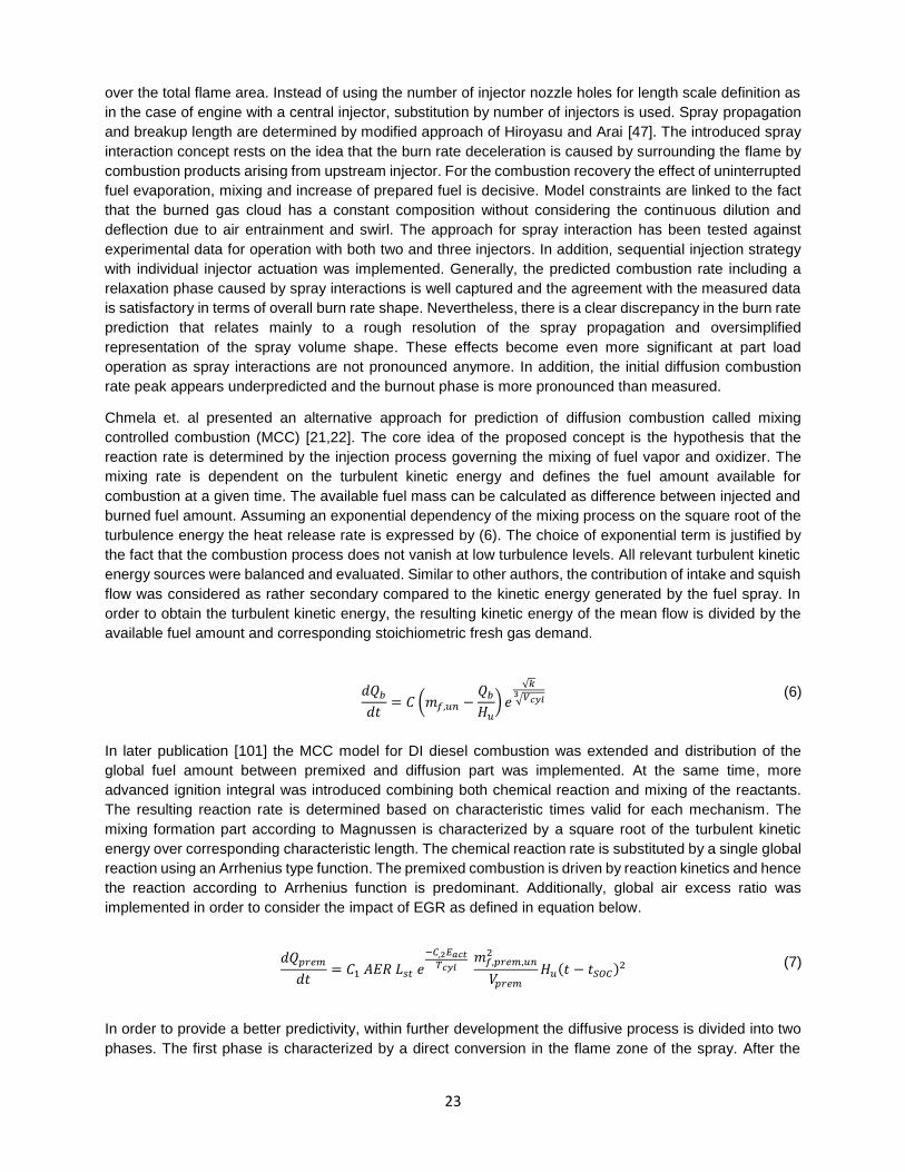
over the total flame area. Instead of using the number of injector nozzle holes for length scale definition as
in the case of engine with a central injector, substitution by number of injectors is used. Spray propagation
and breakup length are determined by modified approach of Hiroyasu and Arai [47]. The introduced spray
interaction concept rests on the idea that the burn rate deceleration is caused by surrounding the flame by
combustion products arising from upstream injector. For the combustion recovery the effect of uninterrupted
fuel evaporation, mixing and increase of prepared fuel is decisive. Model constraints are linked to the fact
that the burned gas cloud has a constant composition without considering the continuous dilution and
deflection due to air entrainment and swirl. The approach for spray interaction has been tested against
experimental data for operation with both two and three injectors. In addition, sequential injection strategy
with individual injector actuation was implemented. Generally, the predicted combustion rate including a
relaxation phase caused by spray interactions is well captured and the agreement with the measured data
is satisfactory in terms of overall burn rate shape. Nevertheless, there is a clear discrepancy in the burn rate
prediction that relates mainly to a rough resolution of the spray propagation and oversimplified
representation of the spray volume shape. These effects become even more significant at part load
operation as spray interactions are not pronounced anymore. In addition, the initial diffusion combustion
rate peak appears underpredicted and the burnout phase is more pronounced than measured.
Chmela et. al presented an alternative approach for prediction of diffusion combustion called mixing
controlled combustion (MCC) [21,22]. The core idea of the proposed concept is the hypothesis that the
reaction rate is determined by the injection process governing the mixing of fuel vapor and oxidizer. The
mixing rate is dependent on the turbulent kinetic energy and defines the fuel amount available for
combustion at a given time. The available fuel mass can be calculated as difference between injected and
burned fuel amount. Assuming an exponential dependency of the mixing process on the square root of the
turbulence energy the heat release rate is expressed by (6). The choice of exponential term is justified by
the fact that the combustion process does not vanish at low turbulence levels. All relevant turbulent kinetic
energy sources were balanced and evaluated. Similar to other authors, the contribution of intake and squish
flow was considered as rather secondary compared to the kinetic energy generated by the fuel spray. In
order to obtain the turbulent kinetic energy, the resulting kinetic energy of the mean flow is divided by the
available fuel amount and corresponding stoichiometric fresh gas demand.
𝑑𝑄𝑏
𝑑𝑡= 𝐶 (𝑚𝑓,𝑢𝑛 −
𝑄𝑏
𝐻𝑢
) 𝑒
√𝑘
√𝑉𝑐𝑦𝑙3
(6)
In later publication [101] the MCC model for DI diesel combustion was extended and distribution of the
global fuel amount between premixed and diffusion part was implemented. At the same time, more
advanced ignition integral was introduced combining both chemical reaction and mixing of the reactants.
The resulting reaction rate is determined based on characteristic times valid for each mechanism. The
mixing formation part according to Magnussen is characterized by a square root of the turbulent kinetic
energy over corresponding characteristic length. The chemical reaction rate is substituted by a single global
reaction using an Arrhenius type function. The premixed combustion is driven by reaction kinetics and hence
the reaction according to Arrhenius function is predominant. Additionally, global air excess ratio was
implemented in order to consider the impact of EGR as defined in equation below.
𝑑𝑄𝑝𝑟𝑒𝑚
𝑑𝑡= 𝐶1 𝐴𝐸𝑅 𝐿𝑠𝑡 𝑒
−𝐶,2𝐸𝑎𝑐𝑡𝑇𝑐𝑦𝑙
𝑚𝑓,𝑝𝑟𝑒𝑚,𝑢𝑛2
𝑉𝑝𝑟𝑒𝑚
𝐻𝑢(𝑡 − 𝑡𝑆𝑂𝐶)2 (7)
In order to provide a better predictivity, within further development the diffusive process is divided into two
phases. The first phase is characterized by a direct conversion in the flame zone of the spray. After the
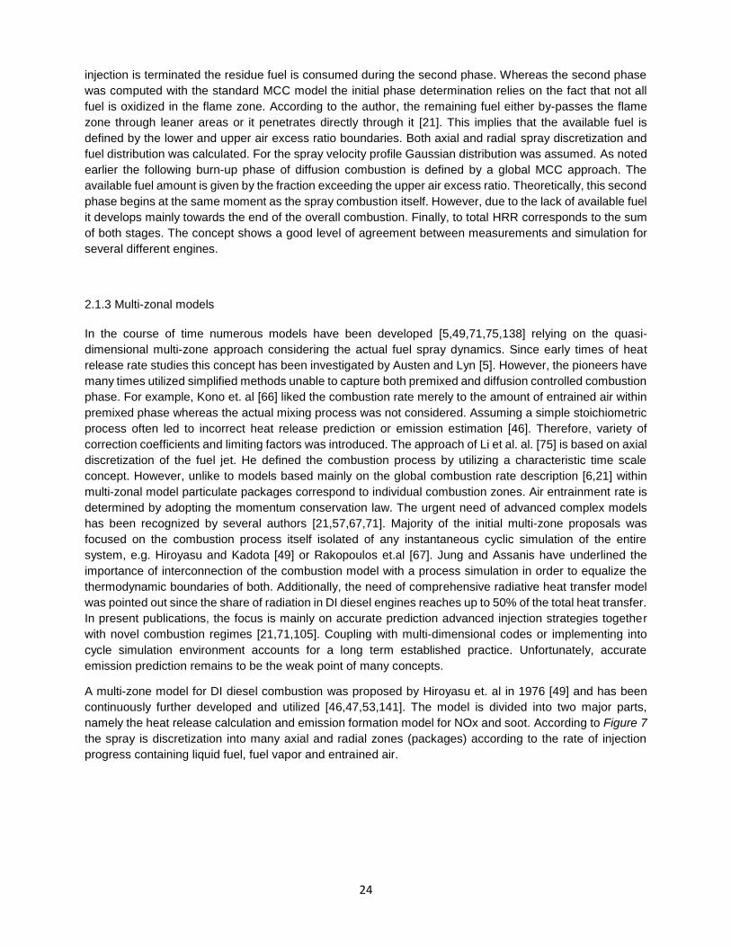
24
injection is terminated the residue fuel is consumed during the second phase. Whereas the second phase
was computed with the standard MCC model the initial phase determination relies on the fact that not all
fuel is oxidized in the flame zone. According to the author, the remaining fuel either by-passes the flame
zone through leaner areas or it penetrates directly through it [21]. This implies that the available fuel is
defined by the lower and upper air excess ratio boundaries. Both axial and radial spray discretization and
fuel distribution was calculated. For the spray velocity profile Gaussian distribution was assumed. As noted
earlier the following burn-up phase of diffusion combustion is defined by a global MCC approach. The
available fuel amount is given by the fraction exceeding the upper air excess ratio. Theoretically, this second
phase begins at the same moment as the spray combustion itself. However, due to the lack of available fuel
it develops mainly towards the end of the overall combustion. Finally, to total HRR corresponds to the sum
of both stages. The concept shows a good level of agreement between measurements and simulation for
several different engines.
2.1.3 Multi-zonal models
In the course of time numerous models have been developed [5,49,71,75,138] relying on the quasi-
dimensional multi-zone approach considering the actual fuel spray dynamics. Since early times of heat
release rate studies this concept has been investigated by Austen and Lyn [5]. However, the pioneers have
many times utilized simplified methods unable to capture both premixed and diffusion controlled combustion
phase. For example, Kono et. al [66] liked the combustion rate merely to the amount of entrained air within
premixed phase whereas the actual mixing process was not considered. Assuming a simple stoichiometric
process often led to incorrect heat release prediction or emission estimation [46]. Therefore, variety of
correction coefficients and limiting factors was introduced. The approach of Li et al. al. [75] is based on axial
discretization of the fuel jet. He defined the combustion process by utilizing a characteristic time scale
concept. However, unlike to models based mainly on the global combustion rate description [6,21] within
multi-zonal model particulate packages correspond to individual combustion zones. Air entrainment rate is
determined by adopting the momentum conservation law. The urgent need of advanced complex models
has been recognized by several authors [21,57,67,71]. Majority of the initial multi-zone proposals was
focused on the combustion process itself isolated of any instantaneous cyclic simulation of the entire
system, e.g. Hiroyasu and Kadota [49] or Rakopoulos et.al [67]. Jung and Assanis have underlined the
importance of interconnection of the combustion model with a process simulation in order to equalize the
thermodynamic boundaries of both. Additionally, the need of comprehensive radiative heat transfer model
was pointed out since the share of radiation in DI diesel engines reaches up to 50% of the total heat transfer.
In present publications, the focus is mainly on accurate prediction advanced injection strategies together
with novel combustion regimes [21,71,105]. Coupling with multi-dimensional codes or implementing into
cycle simulation environment accounts for a long term established practice. Unfortunately, accurate
emission prediction remains to be the weak point of many concepts.
A multi-zone model for DI diesel combustion was proposed by Hiroyasu et. al in 1976 [49] and has been
continuously further developed and utilized [46,47,53,141]. The model is divided into two major parts,
namely the heat release calculation and emission formation model for NOx and soot. According to Figure 7
the spray is discretization into many axial and radial zones (packages) according to the rate of injection
progress containing liquid fuel, fuel vapor and entrained air.
25
Figure 7 Multi-zone discretization of the DI diesel fuel spray according to [50] in axial and radial directions
In late 70’s the solution could be obtained merely on large computer systems. The number of individual
zones or so-called packets depends on the injected fuel mass. In the early publications a time step of single
degree crank angle was used. For a typical injection period duration about 250 elements were generated.
Within each packet temperature and composition history is tracked both for liquid and gaseous components.
Consequently, mass and energy conservation equations are solved. Interactions between the individual
subzones allowing mass and energy exchange are not considered. Diffusion combustion rate is controlled
by fuel vaporization and air entrainment rate which is proportional to the reduction of the package velocity.
Swirl motion in the combustion space has been considered as well. Original correlations for spray
penetration and dispersion were based on their constant volume vessel experiments. The process of air-
fuel mixing takes place in each single zone individually. Droplet size distribution is substituted in a common
way by a Sauter mean diameter characteristic for each packet. The actual size is related to injection
pressure, ambient pressure, fuel kinematic viscosity, surface tension and nozzle diameter. As the packages
propagate into the combustion space the fuel begins to vaporize and surrounding gas is entraining into the
zones. This causes a rapid expansion of the zones and speeds up the evaporation process. The ignition
delay is modeled by means of Arrhenius function including the actual air excess ratio. In more recent
publications [53,141] a flammability limit was implemented so that the combustion launches only if the
mixture in the package is within the range defined by lean limit and rich limit of the air excess ratio. This has
been introduced primarily in order to avoid any temperature overestimation and thus high computed NOx
level. However, the physical significance of such measure is self-evident. Two possible combustion modes
were defined. After ignition, the prepared mixture burns in a short period of time and the heat release rate
is computed under stoichiometric conditions. If the air excess in the package becomes sufficient, the
combustion is controlled by evaporation rate of the fuel. As soon as the lack of oxidizer is recognized to
burn all available fuel within individual packages the combustion is switched into the entrainment rate
controlled mode. The overall burn rate is then calculated by summing up the local heat release rates in all
packages. NOx formation was calculated by using the extended Zeldovich’s mechanism. Soot formation
was determined by first-order reaction of available fuel and soot oxidation by second-order reaction for soot
and oxygen. Initial experiments were performed on a single-cylinder DI diesel engine [141], in more recent
publications series heavy duty engine was used [50]. Predictivity of the heat release rate was in a good
agreement, whereas the estimation of pollutant formation showed merely acceptable outcome.
The main publicity to the approach of Hiroyasu et. al among simulation expert were given by the work of
Morel and Wahiduzzaman [86] by implementing it into a 1-D simulation software for cycle simulation. The
proposed represents the whole range of in-cylinder process by sub-models for fuel jet development,
breakup, air entrainment, evaporation, ignition and emission formation as proposed in [141]. The fuel jet is
divided up to 1500 hundred zones tracked simultaneously. Main advantage compared to CFD codes is a
simplified jet motion correlation compared to detailed solution of entire flow-field. In order to overcome the
main drawbacks of the phenomenological model an integrated tool was introduced in [63] combining both
1-D and 3-D simulation methods, namely GT-SUITE and KIVA-3V. The fuel injection system was modeled
in 1-D environment whereas the combustion and emission formation was done by multi-dimensional CFD
for investigation of transient behavior. This approach has shown good agreement compared to stand-alone

26
CFD simulation and considerable simulation time savings. However, the assessment of the purely
phenomenological combustion was out of scope of the study. All in all, it is fair to state that despite the
variety of publications and integration into commercial software the multi-zone phenomenological approach
according to Hiroyasu et al. [47,138] has not been widely used as a standard tool in development and
optimization process throughout the industry due to a relatively high calibration demand and moderate
benefits.
Figure 8 Discretization of the DI diesel spray proposed by Kuleshov [71] for spray penetration and impingement
A multi-zone model for DI diesel engines has been proposed by Kuleshov [70,71,72] dividing the spray in
several zones inclusive the wall and piston interaction consideration. Transient spray propagation is taken
into account in a turbulent flow field with swirl enabling both central and non-central configuration of injector
position. Additionally, a NOx formation model based on detail kinetic mechanism was implemented. Later
the concept has been extended for HCCI combustion modeling. In the so-called Diesel-RK model the zones
are distributed according to the characteristic air excess ratio. In case of a free spray development during
the initial phase, three zones are formed as shown in Figure 8: 1 - dense axial spray core, 2 - dense fore
front and 3 - diluted spray envelope where the mixing process takes place. As soon as the spray tip impinges
the wall the structure became inhomogeneous and the zonal distribution had to be updated as follows: 4 –
axial conical core, 5 – dense core spread on the piston, 6 – dense front and 7 – diluted area. The distribution
of the fuel among individual zones is governed by utilization of penetration length, break
up time, dense front width and empirical coefficient. Evaporation is determined by D2-law in a similar way
as in [6]. Assuming relative uniform character of spray atomization, Sauter mean diameter is used for
defining the droplet size. For each zone, specific evaporation constant is calculated depending on Nusselt
number, diffusion factor as well as thermodynamic conditions. For cases near to the wall the Nusselt number
is linked to the surface shape resulting in either laminar or turbulent flows. Empirical correction function
based on investigations on various engines was proposed depending on i.a. swirl, engine speed or Sauter
mean diameter. The heat release process is split in four main phases consisting of ignition delay, premixed
phase followed by diffusion phase and, last but not least, the afterburning phase as the injection process is
already terminated. Ignition delay is based on Arrhenius approach according to (8) and is computed for each
portion of fuel in case of multiple injection strategy.
𝜏𝑖𝑔 = 3.8 ∙ 10−6(1 − 1.6 ∙ 10−4𝑛) (
𝑇𝑐𝑦𝑙
𝑝𝑐𝑦𝑙
)
𝑚
𝑒𝐸𝑎𝑐𝑡
8.312∙𝑇𝑐𝑦𝑙𝐶𝐶𝐶𝑇 (8)
Various ignition models were evaluated and compared by the author. In the latest publications [32, 33] a
detailed approach with tabulated chemical reactions generated in CHEMKIN for both low and high
temperature combustion modes. By post-processing the result an empirical equation was derived for ignition
delay of the premixed phase considering the delay of the high temperature phase together with EGR fraction
[71]. The premixed combustion takes place only if the ignition delay is shorter than the one of the diffusion

27
phase. This represents a certain drawback in respect of restriction of reciprocal interactions between both
phases and thus is not fully in accordance with the real process. Low temperature combustion (LTC) part
was approximated by the Vibe function whereas the maximum burned fuel fraction within this mode is given
by an empirical relation.
𝑥𝐿𝑇𝐶 = (0.102 − 0.0392 ∙ 𝑥𝐸𝐺𝑅 ) (
81.6
𝑒∆𝜑𝐿𝑇𝐶−
8.88
∆𝜑𝐿𝑇𝐶
+ 1.2261) {1 − 𝑒(−2.9957(
𝜑𝜑𝑑𝑢𝑟
)𝑚+1
)} (9)
𝑑𝑥𝑑𝑖𝑓
𝑑𝑡=
1(𝑑𝜎𝑢
𝑑𝑡 ) +
2𝐶2 (
𝑚𝑓
𝑉𝑐𝑦𝑙
)(𝑚𝑓,𝑒𝑣𝑎𝑝
𝑚𝑓
− 𝑥)(1
𝐴𝐹𝑅− 𝑥) (10)
In the equation (9) the limit ignition delay LTC was set to 6.7°CA and dur equals to the maximal duration
of the premixed combustion lying in the interval between 6 - 8°CA. The diffusion combustion model is based
on an adopted approach shown in (10) where the factor describes the completeness of fuel vapor
combustion in the particular zones. In similar way, the formula for the last phase of slow afterburning was
derived. The proposed model was implemented into a full-cycle thermodynamic engine simulation software
DIESEL-RK designed by author. Presented results for a high speed DI diesel engine with multiple injection
patterns and moderate EGR demonstrate good agreement with measurements.
Another comprehensive approach was presented by Jung and Assanis [57] dealing with a multi-zone
combustion modeling aimed for compression ignited direct injection (CIDI) diesel engine. Mechanisms for
NOx and soot pollution formation were implemented by means of extended Zeldovich’s scheme and concept
proposed by Hiroyasu, respectively. Fuel spray was split among individual parcels both in axial and radial
direction as evident from Figure 9.
Figure 9 Radial and axial distribution of the fuel spray for DI diesel multi-zone combustion model [57]
Discretization in radial direction was fixed, in the spray direction it depends on the injection duration.
Sensitivity study done by the author has shown that at least five radial zones are prerequisite to achieve
acceptable model accuracy. Each parcel tracks his temperature, pressure and composition. Mass transfer
among individual parcels is not permitted. Mass and energy equation are solved in each individual zone.
For determining the air entrainment, a simplified momentum conservation law was applied assuming that
along the penetration length the initial momentum remains constant. Spray penetration before and after the
breakup time are deterimed according to Hiroyasu and Arai [47]. However, the equations were adapted for
a general use with nozzle discharge coefficient as a free variable instead of a fixed constant. Empirical
correlation for the spray angle based on investigation of Reitz and Bracco [104] showed better agreement
with the experimental observation while the other concept [47] predicts much wider spray shape than
measured. After the breakup time elapses the droplets are assumed to be formed with diameter
corresponding to SMD neglecting the actual droplet size distrubution. Merely the amount of injected fuel
during each time step is governing the resulting droplet size. The rate of evaporation is determined based
on both vapor diffusion away from the droplet and degree of heat transfer. Ignition delay time is calculated
(11)
28
by using an Arrhenius expression. After the treshold for the ignition is reached the evaporated fuel is oxidized
during the first combustion phase under premixed conditions. The corresponding burn rate is determined
by (11) where mass fractions of available fuel vapor and oxygen are included and Tzone and Vzone are the
temperature and volume of the relevant zone.
𝑥𝑝𝑟𝑒𝑚 = 𝐶𝑝𝑟𝑒𝑚𝑥𝑓,𝑣𝑎𝑝𝑥𝑂2𝑒
(−1200𝑇𝑧𝑜𝑛𝑒
)𝑉𝑧𝑜𝑛𝑒 (11)
Conseqently, the diffusion phase follows where the mixing mechanism is assumed to be the limiting factor
whithout any additional restrictions represented by chemical kinetics. However, at the late phase of
afterburning this phenomena gains in importance. Therefore, the diffusion part is defined as a combination
of the instantaneuosly available fuel vapor and a Arrhenius term according to equation (12) where pO2
accounts for partial oxygen pressure, p for total pressure and mf,vap is the fuel vapor mass.
𝑥𝑑𝑖𝑓𝑓 = 𝐶𝑑𝑖𝑓𝑓𝑚𝑓,𝑣𝑎𝑝
𝑝𝑂2
𝑝𝑝0.25𝑒
(−2500𝑇𝑧𝑜𝑛𝑒
) (12)
Validation of the proposed approach has been carried out under various loads, speeds and injection
conditions on single- and multi-cylinder medium speed heavy duty diesel engines. For the selected cases
the model has proved to achieve good agreement with the experimental results in terms of heat release and
predicted NOx and soot emissions. Relatively rough time step of 1°CA was utilized during the study which
indicates a low computational demand of the suggested model.
An alternative phenomenological modeling approach utilized mainly in 3D CFD calculations has been
proposed to be integrated in a 0D phenomenological model for Diesel combustion featuring multi-injection
strategies [82]. A statistical method based on a probability density functions (PDF) was proposed to
characterize the mixture formation. Furthermore, this process has been coupled with a detailed tabulated
chemistry approach for modeling the combustion kinetics which makes the concept capable to simulate
various combustion strategies such as cold flame HCCI concept. Evaporation is assumed to take place at
thermodynamic equilibrium and calculated by means of characteristic evaporation time according to Siebers
[110]. Spray penetration length as well as the spray angle are computed in accordance with [88]. The rate
of air entrainment is derived from the spray development history defining the injection volume, ambient gas
density and the geometrical dependencies individually for each injection. Kinetic turbulent energy is
computed according to a simplified k- approach and analog to [73] other sources except for the fuel injection
spray have been neglected. 0D PDF-based concept was utilized for determining the mixture formation. For
that purpose, a PDF function was selected describing the actual fuel fraction distribution as well as
temperature and species reaction rate. Initially, the field defined by two scalars is completely segregated
since no mixing occurs. At a certain time, all components are mixed and the function converts to a Gauss-
shaped distribution. Under assumption of complete homogenization, the entire zone is represented by a
constant air-fuel ratio. Generally, an application of a probability density function methodology allows tracking
various variables and species. On the other hand, its shape flexibility is restricted by the fact that for its
definition only two parameters are used in presented case, namely the equivalence ratio and the EGR molar-
fraction. In equation (13) the variable Z defines the fuel mass fraction distribution based on PDF.
𝑍 = (
𝑚𝑓
𝑚𝑎𝑖𝑟
)𝑠𝑡
(1 − 𝑥𝐸𝐺𝑅
𝑀𝐸𝐺𝑅
𝑀𝑚𝑖𝑥
)1
(𝑚𝑓
𝑚𝑎)𝑠𝑡
+ 1 (13)

29
For combustion calculation diesel fuel was substituted by n-heptane. Detailed kinetics was defined by four
major reactions including species that are characteristic for the initial mixture composition (O2, CO2, CO, H)
as a function of thermal and chemical state. In order to generate necessary look-up tables, input parameters
such as pressure, temperature, equivalence ratio and EGR were varied. Reaction chemistry was computed
in CHEMKIN environment. Based on those reaction rates and balance equation rates for C7H16, H2O, H2
and N2 were determined. The change of mass fractions of individual species assigned to burned zone
governs the resulting heat release rate. Model validation under various engine speeds, loads, EGR and
injection patterns was performed [29,82] showing satisfying agreement of simulated and measured cylinder
pressure curves.
Resembling the proposal of [82] a novel combustion model utilizing the PDF approach enabling to consider
local inhomogeneity has been developed by Inagaki et al. [54]. The combustion space with centralized
injector is divided into three main zones whereas two additional zones are introduced to represent first and
second pilot pre-injections if applicable as illustrated in Figure 10. Zone 2 accounts for the surrounding gas
and the spray jet is divided into premixed zone 1 and diffusion zone 3, respectively.
Figure 10 Scheme of the zonal distribution in case of multiple injection [54]
Low temperature combustion taking place in zone 1 is limited by authors to 1000K is relies on the Shell
model [41] comprising of eight major reaction equations. Combustion above 1000 K is derived from a laminar
turbulence characteristic time approach according to [65]. Turbulent kinetic energy and its dissipation are
calculated assuming the spray jet and in-cylinder swirl level as the main turbulence sources. The entrained
air volume into the diffusion zone is calculated using the approach proposed by Hiroyasu and Arai [47]. The
actual spray jet shape is simplified by form of a circular cone. If the pre-injection strategy is applied, the
resulting gas composition either burned or only premixed are partially involved in the entrained gas for
premixed and main diffusion combustion and thus affect the subsequent ignition delay. In order to capture
the heterogeneous fuel concentration distribution within the spray, PDF function is directly linked to the
zonal model and is applied to all active zones individually. Each zone is divided into number of spherical
packages containing initially either fuel or surrounding gas. During the mixing process new zones are formed
adopting conservation of mass, momentum and enthalpy. All possible package combinations are resolved
at every time step. Subsequently, the PDF characteristic determines the most likely distribution within
individual zones as shown in Figure 9. For NOx formation extended Zeldovich mechanism was implemented
and applied to each package individually. Finally, integration into commercial 1D cycle simulation software
GT-Suite was done. Comparing the simulation results with experiments on a single-cylinder high speed DI
diesel engine under various loads, EGR rates and injection settings has proved a good accuracy. Predictivity
level of multi-injection patterns and HCCI combustion was also at very good level. Additionally, a transient
process of switching from conventional Diesel combustion to HCCI mode has been modeled with satisfying
outcome. Merely the NOx formation estimation has shown deviations from measurements. All in all, a useful
optimization tool has been developed and validated for a wide operational range. However, it has to be

30
stated that in case of present study with several decentralized injectors and where the diffusion flame is
predominant and thus the in-cylinder turbulence accounts for the major combustion driver a PDF concept
might not be a preferable solution due its extensive complexity and computational demand.
2.1.4 Multi-dimensional Models
Multi-dimensional approach represents the most extensive, generic and interdisciplinary way for predictive
stand-alone combustion modeling. Although it falls outside the scope of the present study it is worthy to
discuss some basic principles. Multi-dimensional models solve multiphase fluid dynamics related to fuel
spray characteristic, turbulent flow field or detailed chemical reaction kinetics. Several approaches were
used to model ignition and combustion process of the diesel fuel, e.g. the eddy dissipation model and its
derivation, coherent flame based models like PDF or RIF (Representative Interactive Flamelet) where
mixture fraction and dissipation rates are solved. In general, scale fluctuations, spatial inhomogeneity,
effects on the boundary layers, turbulence and compressibility have to be considered by any comprehensive
combustion model. In-cylinder processes are characterized by wide range of time and length scales, and
hence a numerical solution is not applicable. In practice, averaged turbulent flow field is utilized in engine
simulation by employment of Reynolds Averaged Navier-Stokes (RANS) transformations which yields to
unclosed parameters defined by additional turbulence models, e.g. k-. An alternative solution method
especially in terms of non-reacting flow applies the large eddy concept (LES/EDC) where merely larger
eddies are computed explicitly [81]. Such approach requires reduced level of empirical input and is capable
of correct in-cylinder flow representation.
Introduction of dedicated CFD tools such as KIVA brought the multi-dimensional combustion simulation by
a substantial step forward. The first proposal for DI diesel combustion modeling was made by Magnussen
[81] employing the eddy dissipation concept (EDC) into a characteristic time scale approach. Key feature of
this method are non-homogenous, localized and intermittent eddies within the diffusion flame both in fine
structures and their surroundings. The turbulent energy from the mean flow is transferred though larger
eddies, whereas the fine structures are determinant for molecular mixing and turbulent energy dissipation.
Interconnection between fine and larger structures is based on turbulence energy cascade model. More
recent concept was reported by Kong et. al. [65] adopting the characteristic time scale as a sum of laminar
and turbulent scales. Laminar part was determined by Arrhenius function turbulent time scale relies on the
k- theory. Assuming local equilibrium combustion is modeled by multi-step reaction scheme. Tanner and
Reitz [118] further developed the characteristic times scale approach by performance evaluation of medium
and low speed DI diesel engines, including 2-stroke SULZER RTA58T. Flow field characteristic relevant to
compressibility and turbulence were captured by the RNG k-ε model. For low temperature reactions were
defined by the Shell model as implemented by Kong [65] in form or Arrhenius type of reaction rate. Although,
the only parameters adjusted for different engines were ignition delay parameter and characteristic time
scale factor the agreement with experiments related to the HRR was on a good level. Merely the interaction
of sprays in case of the SULZER RTA58T could not be approximated accurately [118]. Another adaptation
of the approach according to Kong et. al. [65] was demonstrated by Weisser [132,133] and validated on a
medium speed diesel engine. Combustion with multiple side injectors in large marine 2-stroke engine was
calculated in KIVA by Imahashi et al [52]. The effects of number of nozzles, horizontal nozzle angles and
swirl ratio on combustion process were evaluated. In particular, it has been shown that the characteristic
double-peak heat release caused by the interference of the burned gas upstream to the unburned fuel from
adjacent injector depends strongly on the number of nozzles and that the horizontal angle impacts the
combustion progress only marginal.

31
2.2 Dual Fuel Combustion Modeling
The need for modeling the dual fuel combustion is evident due to the increased interest in dual fuel engines
characterized by flexible operation on both gaseous and liquid fuels. Over the past decades, significant
progress has been made in developing comprehensive simulation techniques of both diffusive and premixed
combustion for reciprocating engine applications. The accuracy of these schemes varies significantly in
complexity depending of computational method and the level of detail. It is worth noting that multi-fuel
combustion concepts were not in the focus due to lack of expertise and lenient environmental regulations.
Hence, much less effort has been invested into associated research and development of suitable simulation
models. Therefore, the state of the art study is rather limited compared to the overview of diesel combustion
modeling presented in previous section.
Deep insights into the problematic of dual fuel combustion of various gaseous fuels and liquid pilot were
prerequisite for concept maturation and successful market introduction. Meanwhile, dual fuel technology is
well proven especially in power generation and marine applications of large medium speed 4-stroke engines
[121]. Designing future solutions cannot rely on experimental studies only. Utilization of various simulation
tools for performing computational analysis is gaining more relevance since they can accelerate the
development process without incurring excessive expenditure. Considering the complexity of the dual fuel
combustion, development of computational models requires a thorough study of individual phenomena and
interactions among them. In order to preserve an adequate level of generality and accuracy physics has to
be taken into account. Of course, the extensive modeling of detailed flow field, turbulence sources and
dissipation and finally the combustion itself as done in CFD cannot be accomplished within a short period
of time required for multi parameter optimizations. On the other hand, even in case of a simplified approach
determinative phenomena cannot be completely neglected since model fidelity over a broad range of engine
operation is desirable. In the present work, small computational demand is desirable for the full engine cycle
simulation while maintaining the effects of the turbulent flow processes and interactions during oxidation of
both participating fuels. This requires considering the spatial non-uniformity in temperature and
concentrations into certain extent.
Parallel to the diesel combustion model classification in previous chapter, approaches for dual fuel
combustion modeling can be distinguished by number of dimensions they account for. In this respect, zero-
dimensional, quasi-dimensional and multi-dimensional models are characterized by increasing proximity to
detailed physics corresponding with the model complexity. A wide spectrum of computational methods has
been utilized in the past, ranging from detailed multidimensional CFD approaches over quasi-dimensional
concepts towards reduced empirical correlations. Zero-dimensional models neglect the spatial differences
in thermodynamic state parameters and often employ ideal gas conditions to calculate overall engine
performance figures. Despite of constraints linked to accuracy and restricted validity they are widely used
due to their simplicity. Further division of zero-dimensional models can be done based on number of zones
defined for the in-cylinder processes. The single zone approach typically incorporates measurement based
heat release rate and the engine is handled as a single thermodynamic system with uniform pressure and
temperature history throughout the cylinder control volume. The transition to two zone model includes
differentiation between unburned and burned zones with characteristic thermodynamic properties. Although
the obtained results are closer to the reality several effects such as interzonal heat transfer or injection
enthalpy are not considered. Quasi-dimensional models improve the fidelity in a way of accounting for
spatial differences in temperature and concentration by conceiving the cylinder charge to be divided into
many zones varying in properties and considering interactions between pilot and main fuels. Multi-
dimensional 3D-CFD models account for energy, mass and momentum balances for individual zones i.e.
cells and resolve the flow field and turbulence in detail. Furthermore, the associated kinetics for both liquid
and gaseous fuel can be considered by using appropriate mechanism for each of them. This allows that
both pilot triggered and autoignition controlled combustion modes (e.g. HCCI) can be simulated in a

32
comprehensive way. These models are being continuously further developed by raising their complexity
and validating the implemented submodels against experimental outcome of basic research.
An inseparable part of low-pressure DF combustion concept is limitation of the maximum achievable brake
mean effective pressure by the knock onset. In fact, the origin of end gas knock is linked to sudden auto-
ignition of unburned mixture prior to arrival of the flame front. Consequently, the explosive combustion of
the remaining unburned fuel leads to extensive pressure oscillations that may trigger severe mechanical
damage of the engine. Therefore, predicting of knock becomes essential engine operation limits prediction.
Merging all chemical reactions into a single global one, an approximation of the knock onset can be
determined by a logarithmic dependency on the temperature of unburned mixture. In dual fuel engines the
knock behavior is related not only to the unburned zone temperature but also to pilot fuel amount, pilot
injection timing and the quality gaseous fuel defined by methane number MN. In conclusion, a simple
approach based on a single global reaction provides only limited predictivity. Alternatively, detailed
mechanism for reaction kinetics can be utilized. Apart of solely DF dedicated computational efforts which
are rather limited the state of the art section covers also publications related to premixed combustion often
formulated for a SI gasoline or gas engine.
Efforts to develop a comprehensive fast running DF combustion model with low pressure gas admission
have been limited due to both complexity and availability of engine related data. Interactions between mixing
controlled pilot fuel combustion and the premixed combustion need to be well understood before deriving a
suitable computational model. Moreover, accurate prediction of micro-pilot ignition at minimum diesel share
presents an additional modeling challenge. One of the first DF modeling efforts was reported by Gao et al.
[35] simulating a diesel engine fumigated with ethanol. Three zone division of the combustion space account
for unburned mixture of air and ethanol, unburned diesel fuel and finally the zone containing combustion
products. Entrainment of diesel and premixed fuel is assumed to be identical independently on the
conditions and thus the predictivity of the model is limited considerably. The objective to predict nitric oxides
therefore also constrained to a narrow engine operation range.
An empirical modeling concept presented by Xu et al. [139] describes both diesel and dual-fuel combustion
process using a triple Vibe function approach. The ignition delay is determined by iterations of SOC and
ignition integral correlation. While maintaining the original diesel engine design with high compression ratio
merely fumigation approach at comparable lower SR due to knock limitation. The main motivation was to
reduced fuel cost while maintaining high thermal efficiency. Compressed natural gas is injected upstream
the intake manifold and the engine was equipped with a variable geometry turbine. The proposed model
was integrated into 1-D GT-Suite simulation environment and used for transient simulations of a heavy-duty
engine with satisfying prediction accuracy.
An advanced technique using empirical functions to avoid non-linear regression of the multiple Vibe
approach and to respect afterburning by a look-up table based reference heat release curve is introduced
in [125] and [112]. The heat release curves are additionally corrected based on specific engine and fuel
features. Such models are very efficient for optimization runs with multiple cases and thus can be easily
implemented into engine cycle simulation software. However, since no physics based submodels are
implemented the lack of generic validity does not allow further application for different engine sizes and
types without substantial modification of the heat release rate maps.
A multi-zone dual fuel model for full load performance and knock predictions was developed by Liu and
Karim [77] using experimental data from a single cylinder engine with 106mm bore and compression ratio
(CR) 14.7 at 1000rpm for validation. The approach is an evolution of the author’s earlier work introducing a
three stage description of the DF combustion process. The model comprises of five individual zones
according to Figure 11 describing the pilot spray regions, reacting zone and unburned gaseous zone.
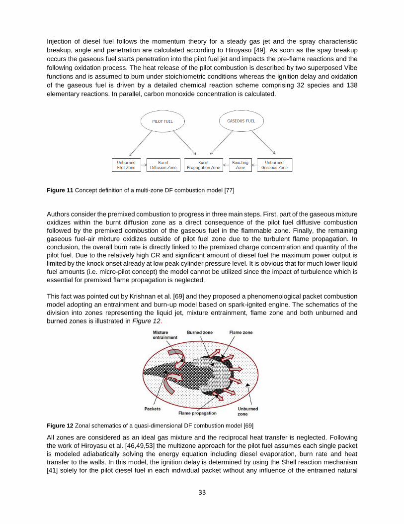
33
Injection of diesel fuel follows the momentum theory for a steady gas jet and the spray characteristic
breakup, angle and penetration are calculated according to Hiroyasu [49]. As soon as the spay breakup
occurs the gaseous fuel starts penetration into the pilot fuel jet and impacts the pre-flame reactions and the
following oxidation process. The heat release of the pilot combustion is described by two superposed Vibe
functions and is assumed to burn under stoichiometric conditions whereas the ignition delay and oxidation
of the gaseous fuel is driven by a detailed chemical reaction scheme comprising 32 species and 138
elementary reactions. In parallel, carbon monoxide concentration is calculated.
Figure 11 Concept definition of a multi-zone DF combustion model [77]
Authors consider the premixed combustion to progress in three main steps. First, part of the gaseous mixture
oxidizes within the burnt diffusion zone as a direct consequence of the pilot fuel diffusive combustion
followed by the premixed combustion of the gaseous fuel in the flammable zone. Finally, the remaining
gaseous fuel-air mixture oxidizes outside of pilot fuel zone due to the turbulent flame propagation. In
conclusion, the overall burn rate is directly linked to the premixed charge concentration and quantity of the
pilot fuel. Due to the relatively high CR and significant amount of diesel fuel the maximum power output is
limited by the knock onset already at low peak cylinder pressure level. It is obvious that for much lower liquid
fuel amounts (i.e. micro-pilot concept) the model cannot be utilized since the impact of turbulence which is
essential for premixed flame propagation is neglected.
This fact was pointed out by Krishnan et al. [69] and they proposed a phenomenological packet combustion
model adopting an entrainment and burn-up model based on spark-ignited engine. The schematics of the
division into zones representing the liquid jet, mixture entrainment, flame zone and both unburned and
burned zones is illustrated in Figure 12.
Figure 12 Zonal schematics of a quasi-dimensional DF combustion model [69]
All zones are considered as an ideal gas mixture and the reciprocal heat transfer is neglected. Following
the work of Hiroyasu et al. [46,49,53] the multizone approach for the pilot fuel assumes each single packet
is modeled adiabatically solving the energy equation including diesel evaporation, burn rate and heat
transfer to the walls. In this model, the ignition delay is determined by using the Shell reaction mechanism
[41] solely for the pilot diesel fuel in each individual packet without any influence of the entrained natural
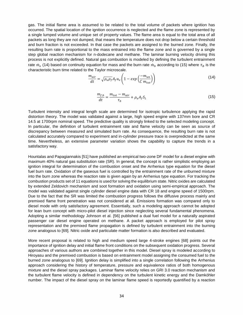
34
gas. The initial flame area is assumed to be related to the total volume of packets where ignition has
occurred. The spatial location of the ignition occurrence is neglected and the flame zone is represented by
a single lumped volume and unique set of property values. The flame area is equal to the total area of all
packets as long they are not dumped, that means the temperature does not drop below a certain threshold
and burn fraction is not exceeded. In that case the packets are assigned to the burned zone. Finally, the
resulting burn rate is proportional to the mass entrained into the flame zone and is governed by a single
step global reaction mechanism for n-dodecane and methane. The laminar burning velocity driving this
process is not explicitly defined. Natural gas combustion is modeled by defining the turbulent entrainment
rate �̇�𝑒 (14) based on continuity equation for mass and the burn rate �̇�𝑏 according to (15) where 𝜏𝑏 is the
characteristic burn time related to the Taylor microscale.
𝑚𝑎𝑖𝑟
𝑑𝑡= √𝜌𝑢𝜌𝑓𝐴𝑓𝑢𝑒 (1 − 𝑒𝑥𝑝 (
−𝑚𝑢𝑛
𝐶 𝑚𝑡𝑜𝑡
)) (14)
𝑚𝑓,𝑏
𝑑𝑡=
𝑚𝑡𝑜𝑡 − 𝑚𝑎𝑖𝑟
𝜏𝑏
+ 𝜌𝑢𝐴𝑓𝑆𝐿 (15)
Turbulent intensity and integral length scale are determined for isotropic turbulence applying the rapid
distortion theory. The model was validated against a large, high speed engine with 137mm bore and CR
14.5 at 1700rpm nominal speed. The predictive quality is strongly linked to the selected modeling concept.
In particular, the definition of turbulent entrainment rate and flame velocity can be seen as source of
discrepancy between measured and simulated burn rate. As consequence, the resulting burn rate is not
calculated accurately compared to experiment and in-cylinder pressure trace is overpredicted at the same
time. Nevertheless, an extensive parameter variation shows the capability to capture the trends in a
satisfactory way.
Hountalas and Papagiannakis [51] have published an empirical two-zone DF model for a diesel engine with
maximum 40% natural gas substitution rate (SR). In general, the concept is rather simplistic employing an
ignition integral for determination of the combustion onset and the Arrhenius type equation for the diesel
fuel burn rate. Oxidation of the gaseous fuel is controlled by the entrainment rate of the unburned mixture
into the burn zone whereas the reaction rate is given again by an Arrhenius type equation. For tracking the
combustion products set of 11 equations is used for solving the equilibrium state. Nitric oxides are calculated
by extended Zeldovich mechanism and soot formation and oxidation using semi-empirical approach. The
model was validated against single cylinder diesel engine data with CR 18 and engine speed of 1500rpm.
Due to the fact that the SR was limited the combustion progress follows the diffusive process mainly and
premixed flame front penetration was not considered at all. Emissions formation was compared only to
diesel mode with only satisfactory agreement. Essentially, such a modeling approach cannot be adopted
for lean burn concept with micro-pilot diesel injection since neglecting several fundamental phenomena.
Adopting a similar methodology Johnson et al. [56] published a dual fuel model for a naturally aspirated
passenger car diesel engine operated on methane. A packet approach is employed for pilot spray
representation and the premixed flame propagation is defined by turbulent entrainment into the burning
zone analogous to [69]. Nitric oxide and particulate matter formation is also described and evaluated.
More recent proposal is related to high and medium speed large 4-stroke engines [68] points out the
importance of ignition delay and initial flame front conditions on the subsequent oxidation progress. Several
approaches of various authors are combined together in this model. Diesel spray is modeled according to
Hiroyasu and the premixed combustion is based on entrainment model assigning the consumed fuel to the
burned zone analogous to [69]. Ignition delay is simplified into a single correlation following the Arrhenius
approach considering the history of temperature, pressure and equivalence ratios of both homogenous
mixture and the diesel spray packages. Laminar flame velocity relies on GRI 3.0 reaction mechanism and
the turbulent flame velocity is defined in dependency on the turbulent kinetic energy and the Damköhler
number. The impact of the diesel spray on the laminar flame speed is reportedly quantified by a reaction

35
mechanism for n-heptane. Nitric oxide formation is calculated by reaction kinetics that capture trends with
a narrow window of varied parameters fairly well. Since no spatial resolution is introduced to the model,
there is no option to capture the location of the actual igniting packet or interaction with the combustion
space walls exists. Except for the premixed peak of the pilot fuel for high SR the model predicts both heat
release and NO formation quite well for the assessed engine types.
An example of a quasi-dimensional two-zone modeling of a SI engine is given in [37] based on entrainment
of eddies from unburned zone to the flame zone and oxidizes upon the burn-up time elapses. Such approach
was employed by various other authors in the past. For instance, Blizard and Keck [9] postulated the
entrainment rate to be proportional to the gas velocity through inlet valves to eliminate the turbulence
solving. Grill et. al [37] further developed the entrainment method of unburned mixture into burned zone that
defines the oxidation rate for a SI engine. The flame propagation is idealized and takes place in a form of
hemispherical area originating from the ignition location. The associated flame surface area is mapped in
dependence of spark plug timing. The resulting burned rate is calculated from the entrained mass into the
flame zone in dependence on the isotropic turbulence speed and the characteristic burn-up time which is
determined by a ratio of Taylor length scale over a laminar flame speed. The laminar flame speed is
calculated according to [44] considering the impact of temperature, pressure, equivalence ratio and the
residual gas fraction. One of the key roles in the model concept constitutes the turbulent kinetic energy
defined for homogenous and isotropic conditions utilizing the k- model. Turbulence production through
cylinder volume change, squish and tumble are considered as shown in equation (16).
𝑑𝑘
𝑑𝑡= −
3
2
𝑘
𝑉𝑐𝑦𝑙
𝑑𝑉𝑐𝑦𝑙
𝑑𝑡− 𝐶𝑑𝑖𝑠𝑠
𝑘3 2⁄
𝑙𝐼+ 𝐶𝑠𝑞𝑢𝑖𝑠ℎ
𝑘𝑠𝑞𝑢𝑖𝑠ℎ3/2
𝑙𝐼
(16)
The overall burn rate calculation relies on characteristic burn-up time determined from ratio of characteristic
length scale over laminar flame speed. For the characteristic length scale Taylor microscale is used. The
modeling approach is validated against natural aspirated and turbocharged gasoline SI engines featuring a
variable valve drive. For different engine types, merely the coefficient defining the initial turbulence value
need to be adjusted leading to an overall good level of predictivity. The model was coupled with 1-D flow
simulation and full engine mapping was performed at good conformity with the measurements. Furthermore,
implementing the knock integral model according to Worret allows using the model for optimization of the
engine efficiency based on controlling the combustion position by 50% MFB point location. The concept
approach for determination of specific turbulent kinetic energy for reduced zero-dimensional models was
further developed by Bargende [7] into a comprehensive form considering except for the compressibility and
squish source terms also contribution of intake flow, piston motion, tumble and dissipative effect due to
vicinity of combustion chamber walls.

36
3. Motivation and Objectives
Summarizing various attempts described in the state of the art section it becomes obvious that a usage of
a standalone empirical model does not suit requirements of the present model aiming for both predictive
physical based combustion modeling in large low speed 2-stroke engine under both diesel and DF
operation. Phenomenological models capture physics with higher fidelity and tend to be generic. However,
the majority comprises set of model constants that need to be tuned based on experimental data or using
multidimensional CFD calculations. Multi-zonal models further extend the capability to account for spatially
resolved effects. Generally, higher complexity of simple zero-dimensional or quasi-dimensional relates to
enhanced demand on model tuning and hence limits the applicability. Moreover, for each engine type and
size such methods have to be reviewed, adapted or even completely redefined and set-up again. Therefore,
employment of existing combustion models for large 2-stroke low speed marine engines is not feasible.
Moreover, the specifics of uniflow scavenging, peripheral diesel fuel injection with multiple injector or direct
gas admission in case of DF version require a new approach considering the spatial differences in
concentration or spray propagation.
In comparison to a broad scope of diesel combustion modeling concepts available in literature, the complex
dual fuel problematic has not been investigated extensively enough in the past. The reason for that is
associated with emission legislative just recently becoming more stringent and economic aspects related to
fuel price. Regardless of the unbalance between existing diesel and dual fuel combustion models, neither
for diesel nor for dual fuel operation comprehensive combustions models have been developed considering
all substantial specifics of large marine 2-stroke engine such as multiple main diesel injectors or direct low-
pressure gas admission. Moreover, based on literature study there is no phenomenological models of dual
fuel combustion in large 2-stroke marine engine at present. Therefore, the demand to develop such a model
for fast running engine performance analysis and optimization is indisputable.
Therefore, the scope and goals of the present work can be outlined as follows:
The main target of the present study is a comprehensive assessment of phenomenological aspects of
combustion in large low speed uniflow scavenged 2-stroke marine engines and the identification of generally
valid concepts for describing diesel and dual fuel combustion in such engines. This comprises the
development of quasi-dimensional, physics-based and fast running combustion modeling methodology in
order to enable engine performance analysis and optimization under both steady state and transient
operation conditions.
Partial aims are related to the limitations of zero-dimensional concepts that can be eliminated by a quasi-
dimensional modeling approach of phenomena that impact the model accuracy substantially. In particular,
spray interactions for the diesel combustion model and gas admission and associated ignition delay in dual
fuel operation are considered. In order to do so, multi-zone models have to be utilized for cylinder volume
discretization, according to the respective needs of the diesel and DF combustion modes.
Validation of individual submodels is done preferably against experimental data, e.g. for diesel spray
propagation and dispersion. The extensive research carried out in parallel on a spray combustion chamber
(SCC) representative of the bore size, injector nozzle geometry and conditions specific for large 2-stroke
marine diesel engines [127,128] has been instrumental in this context. However, due to the lack of specific
experiments related to the respective phenomena, selected submodels need to be compared to
multidimensional CFD simulation results. The final combustion models are validated against full scale

37
engine data at various operating conditions and for different engine bore sizes. The number of engine type
specific constants is intended to be minimized for the sake of generic model validity.
The models shall be integrated into the commercial 1D cycle simulation tool GT-Suite for both combustion
scenarios by means of a user routine. In this way, a direct link between the routine and in-cylinder
thermodynamics and engine performance can be established. Finally, the model capabilities for combustion
prediction and engine performance optimization are to be demonstrated in case studies for transient engine
loading and for integrated marine propulsion systems.

38
4. Theory
4.1 Thermodynamics
A thermodynamic system is characterized by definite number of independent state variables, i.e. pressure,
volume and species concentration represented by a mole number. The temperature of the system is defined
by the independent variables through the equation of state, which in case of ideal gas yields
𝑝𝑉 = ∑𝑛𝑖𝑅𝑇
𝑖
(17)
Apart from thermodynamic quantities comprising temperature, pressure and density, the instantaneous
state of a viscous compressible fluid is determined also by corresponding velocity components ui. Governing
equations for fluid dynamics are developed from balancing basic laws of conservation of mass, momentum
and energy over an arbitrary control volume. The general form valid definition for conservation equation of
a random, volume specific quantity balanced over volume V is expressed by equation (18). The temporal
change of the balanced quantity is given by convective fluxes relatively to the boundary velocity ubound,
surface sources s,surf involving molecular diffusion, heat conduction or viscous forces and volume sources
s,vol taking into account e.g. gravity or chemical energy due to combustion.
𝑑
𝑑𝑡∫ 𝑑𝑉 = − ∮ (�⃗⃗� − �⃗� 𝑏𝑜𝑢𝑛𝑑) �⃗� 𝑑𝑆 + ∮𝑠 𝜑,𝑠𝑢𝑟𝑓 �⃗� 𝑑𝑆
.
𝜕𝑉
.
𝜕𝑉
.
𝑉(𝑡)
+ ∫ 𝑠𝜑,𝑣𝑜𝑙 𝑑𝑉
.
𝑉(𝑡)
(18)
The general form of conservation equation can be transformed into a differential form using Gauss theorem
for replacing surface integrals and assuming that time derivative of sum is equal to the sum of the time
derivatives. Therefore, the compact form for conservation of a generic quantity representing a vector of
gas properties can be expressed as follows:
𝜕
𝜕𝑡+ ∇(𝐹 + 𝜑𝑉) − 𝐻 = 0 (19)
where F and V denote fluxes of the balanced quantity without and with fluid transport respectively and H
represents source or sink term. In order to derive conservation of mass from the equation (18) is to be
substituted by density whereas both flux without mass transport and source terms remain zero.
𝜕
𝜕𝑡+
𝜕
𝜕𝑥𝑗
(𝜌𝑢𝑖) = 0 (20)
Analogous to the equation of continuity, conservation of momentum corresponds to formulation of Navier-
Stokes equations:
𝜕
𝜕𝑡(𝜌𝑢𝑖) +
𝜕
𝜕𝑥𝑗
(𝜌𝑢𝑖𝑢𝑗) = −𝜕𝑝
𝜕𝑥𝑖
+𝜕𝜏𝑖𝑗
𝜕𝑥𝑖𝜕𝑥𝑗
+ 𝑓𝑖 (21)
where the terms on the left side stand for of time-dependent and convective acceleration, whereas the right
part accounts for pressure gradient, viscosity and body forces. The impact of body forces such as gravity

39
applies mainly for liquid fluids and can be largely neglected in aerodynamics. Convective acceleration is
strongly non-linear spatial effect occurring also in a steady flow for instance in a decelerating flow though
nozzle. Merely in case of one-dimensional incompressible flow the convective acceleration is not
considered. For Newtonian fluid viscous stresses linked to its flow and responsible for its deformation is
approximated by a strain rate which is in turn dependent on the velocity vector changes. It is often useful to
define conservation of energy by using specific enthalpy h=cpT according to (22). On the right hand side of
the equation the first two terms stand for material derivative of pressure followed by heat flux term as a
consequence of conduction governed by the Fourier law relation. The fourth term represents a dissipation
function which accounts for energy dissipation due to the viscosity. For combustion applications a source
term needs to be added in order to account for the resulting heat flux due to exothermic chemical reactions.
𝜕
𝜕𝑡(𝜌ℎ) +
𝜕
𝜕𝑥𝑗
(𝜌ℎ𝑢𝑗) =𝛿𝑝
𝛿𝑡− 𝑢𝑗
𝜕𝑝
𝑥𝑗
+ 𝜏𝑖𝑗
𝜕𝑢𝑖
𝜕𝑥𝑗
−𝜕𝑞𝑗
𝜕𝑥𝑗
(22)
Applying fundamental laws of thermodynamics on zero-dimensional open thermodynamic system
representing the engine several assumptions and adaptations have to be made [79]. In addition to quantities
of state the open system with periodic gas exchange is characterized also by masses and concentrations
of all species. Hence, the conservation law has to be extended by the energy transported by the fluid.
Interpretation of the conservation of energy for internal combustion engines yields differential form where
dQ/dt is the heat flux, U is the internal energy of the fluid, h = u + pv is the specific enthalpy and P mechanical
power.
𝑑𝑄𝑖𝑛
𝑑𝑡−
𝑑𝑄𝑜𝑢𝑡
𝑑𝑡+
𝑑𝑚𝑖𝑛
𝑑𝑡ℎ𝑖𝑛 −
𝑑𝑚𝑜𝑢𝑡
𝑑𝑡ℎ𝑜𝑢𝑡 =
𝑑𝑈
𝑑𝑡+ 𝑝
𝑑𝑉
𝑑𝑡+ 𝑃 (23)
4.2 Turbulence
Turbulent flow is characterized by random velocity fluctuations in all directions with infinite number of scales.
The flow is three dimensional with non-zero vorticity, chaotic, diffusive, dissipative, and intermittent i.e.
discontinuous. Within turbulent flow fields vortex stretching introduces the essential principle of eddies
depletion initiated from the large integral scales constrained by the system layout down to the smallest
Kolmogorov microscales forming the viscous sub-layer where the kinetic energy dissipates into thermal
energy. Due to its complexity, an exact description of turbulent flow is generally not feasible. Hence,
statistical characterizations using mean component of fluctuating variables, mathematical correlations or
probability density functions are being employed for approximation. With respect to a combustion process,
turbulence effects intensify mass and heat transport across the flame boundary which improves the mixing
and finally enhances fuel oxidation.
The transition from laminar to turbulent flow regime is promoted when inertial exceed viscous forces within
the fluid. For turbulence level characterization Reynolds number Re is determined as a ratio of inertial to
viscous forces. In a turbulent flow, inertial forces responsible for formation of flow instabilities prevail which
leads to high Reynolds number. On the other hand, domination of viscous forces results into a laminar flow.
Besides to density and dynamic viscosity flow velocity and characteristic dimension D are included in the
definitional relation for Reynolds number (24).
𝑅𝑒 =
𝜌𝑢𝐷
𝜇=
𝑢𝐷
(24)

40
Numerical solution of turbulent flow field requires a physical and mathematical model for resolution of non-
linear conservation equations where the individual variables account for random irregular values both in
time and space. Therefore, an exact solution of Navier-Stokes is impracticable and is usually substituted by
an approximation relying on a statistical approach. For turbulence description it is favorable to employ mean
parameters of the flow. In practice, two fundamental philosophies are typically employed. The first concept
rests on Direct Numerical Solution (DNS) of governing equations taking into account all physical length
scales. Such method prerequisites a dense computational mesh with number of knots proportional to
roughly third power of Reynolds number and thus its applications are limited to elemental problems with
lower Reynolds numbers and simple geometry. Second concept called Reynolds Averaged Navier-Stokes
(RANS) is based on decomposition of instantaneous variables into a mean value and its fluctuating
component. The system of equations resolves merely the mean flow field and for closure model of
turbulence is necessary. Large Eddy Simulation (LES) introduces a compromise between both methods
mentioned above simulating the turbulent transport of mass, momentum and energy in large eddies. The
basic equations are given by applying a filter function selecting larger eddies at the level of computational
grid size. The motion of small eddies is superposed and modeled by a subgrid model resembling the
statistical methodology of turbulence.
Mostly adopted turbulence models for engineering problems are based on RANS concept due to benefits
related to computational time and sufficient information about the mean flow properties. Convenient way for
describing vorticity has been established by splitting the instantaneous value of the turbulent flow quantity
in to a mean component and its corresponding fluctuation. The value of the mean component is given by
averaging selective functions interpreting the random process.
(𝑥, 𝑡) = ̅(𝑥, 𝑡) + ′(𝑥, 𝑡) (25)
Implementation of Reynolds decomposition (25) leads to modified conservation equations consisting of
mean quantities and the fluctuating terms. Terms involving density fluctuation lead to significant
complication of the solution. Substitution of instantaneous flow variables by the sum of mean value and its
fluctuation using presented decomposition rule the Navier-Stokes definition (21) is transformed as follows:
𝜕
𝜕𝑡(�̅��̃�𝑖) +
𝜕
𝜕𝑥𝑗
(�̅��̃�𝑖�̃�𝑗 ) = −𝜕�̅�
𝜕𝑥𝑖
+𝜕
𝜕𝑥𝑖𝜕𝑥𝑗
(𝜏𝑖𝑗 − 𝜌𝑢′𝑖𝑢′𝑗̅̅ ̅̅ ̅̅ ̅̅ ̅) (26)
The 𝜌𝑢′𝑖𝑢′𝑗̅̅ ̅̅ ̅̅ ̅̅ ̅ term on the right side representing the impact of turbulent fluctuations on the momentum
transfer within the fluid. This component stands for Reynolds stresses and contains fluctuations both of
density and viscosity. Except for governing equations and constitutive relations an additional closing term
has to be added to the numerical system. Then, the solution is determined for the transport of the turbulent
stresses and fluxes by using a suitable turbulence model. In regard to complexity, turbulence models can
be divided into two main categories.
The first order models i.e. algebraic and one-equation and partly also two-equations approaches rely on the
Boussinesq approximation concept [15] utilizing a direct analogy between viscous stresses in laminar flows
and turbulent Reynolds stresses. A simple algebraic model does not contain any additional transport
equation that would derive turbulent viscosity from mean flow quantities. The turbulent velocity which is
comparable to the eddy fluctuating velocity term is defined by solving the transport equation for turbulent
kinetic energy. In case of length scale determining the solution is not trivial. Nevertheless, for elementary
one-dimensional flow an assumption of length scale proportional to the normal distance to the wall can be
made. Although attempts for extension on three-dimensional problems have been done general applicability
of this approach is rather limited.
41
Second order models are based on direct solving transport equations for second order moments, i.e.
Reynolds stresses and fluxes aiming to improve predictive capabilities for cases where first order methods
are not convenient enough. Therefore, additional exact transport equations are derived for the emerged
unknown terms. This approach can be practiced only to a certain extent and followed by approximation of
unknown correlations. Such models are denoted Reynolds Stress Models (RSM) since in the most cases
merely transport equations for Reynolds stresses are solved. Unlike the eddy viscosity approximation where
assumption for local isotropy and equilibrium restricts its applicability, RSM methods are well suited for flow
fields with transient changes with rotation or stratification including complicated geometry and spatial flows.
Exact solution of Reynolds stresses allows the model to respond to flow characteristics such as rotation or
buoyancy. Due to determination of additional transport equations apart from those for turbulent kinetic
energy and dissipation rate computational demand rises significantly. A simplifying alternative is an
algebraic stress model (ASM) where the components for calculation Reynolds stresses are based on
algebraic relation. These models rely on the fact that the turbulent stresses relatively to turbulent energy
across a thin shear layer remains nearly constant.
The most commonly used approach is the two-equation model characterized by two transport equations for
both turbulent (integral) and length scales. This approach represent an intermediate path between both
methods introduced previously. Besides the relation for turbulent kinetic energy k that represent the total
mass related energy of the turbulent flow field the rate of turbulent energy dissipation is modeled using
characteristic length scale depending on the flow. Among others, k- model is widely used due to its time
effectiveness and relative simplicity. It is based on transport models for Reynolds stresses and fluxes in
dependency of the turbulent kinetic energy k (TKE) according to (27) where u’, v’, w’ are the turbulent
intensities in individual direction defined as a standard deviation of the velocity fluctuations. For isotropic
conditions fluctuations in all orientations are assumed to be identical so that TKE can be expressed only by
a dependency on u’.
𝑘 =
1
2(𝑢′2 + 𝑣′2 + 𝑤′2) =
3
2𝑢′2
(27)
TKE production is related to fluid shear, friction or buoyancy and to external sources acting at large eddies
at integral scale. The transport differential equation for the turbulence kinetic energy denoted by k can be
derived from conservation of momentum in the following form:
�̅�
𝜕�̃�
𝜕𝑡+ �̅��̃�𝑗
𝜕�̃�
𝜕𝑥𝑗
= 𝜏𝑖𝑗
𝜕�̃�
𝜕𝑥𝑗
− �̅�휀̃ +𝜕
𝜕𝑥𝑗
[(𝜇 +𝜇𝑡
𝜎𝑘
)̅̅ ̅̅ ̅̅ ̅̅ ̅̅ ̅ 𝜕�̃�
𝜕𝑥𝑗
] (28)
where the local temporal change and convection of the TKE on the left side are driven by the production,
dissipation and diffusion terms on the right including an empirical model constant k. In order to solve the
closure problem, the transport equation has to be completed by a turbulence model for turbulent stress
tensor 𝑖𝑗, transport gradient, turbulent eddy viscosity 𝜇𝑡 and mixing length. Analogically, the transport
equation for dissipation can be derived as presented in [102]. For isotropic conditions, the dissipation rate
is defined as decay of the turbulent kinetic energy over the time. Assuming decomposition of the
representative largest eddy with the characteristic length scale lI and kinetic energy proportional to the
square of turbulence intensity, the dissipation rate can be approximated by the following relation.
휀 = −
𝜕𝑘
𝜕𝑡~
𝑢′2
𝑙𝐼/𝑢′=
𝑘3/2
𝑙𝐼
(29)
An immense number of length, time, and velocity scales characterize turbulent flow fields. Within this field
vortex stretching introduces an essential principle for the energy cascade concept which assumes thinning

42
of the particular eddies from the initial large integral scales constrained by the physical boundaries of the
down to the smallest microscales forming the viscous sub-layer. The largest vortex size can be determined
by a simplified two-dimensional analysis using a two points correlation. Assuming the vortex moves from
the distinct spatial location x0 to another position distant from the initial location by x, the velocity components
sampled at both positions are expected to correlate. In case the distance x is larger than the eddy size, this
correlation is not valid. Thus, the size of the large turbulent eddies can be determined by an integral of the
velocity components ratio of two distinct points along the distance between them as defined below.
𝑙𝐼 = ∫
∆𝑢(𝑥0) ∙ ∆𝑢(𝑥0 + 𝑥)
𝑢′(𝑥0) ∙ 𝑢′(𝑥0 + 𝑥)𝑑𝑥
∞
0
(30)
Theoretically, for each velocity component three length scales in each direction could be defined. However,
for isotropic and homogenous turbulence are the longitudinal scales larger than transverse integral length
scales by factor two. In conclusion, merely a single integral length scale is used for representation of the
large eddies and thus the link to the effect of turbulence spectrum shift towards smaller eddy sizes during
the turbulence decay. Based on the mean velocity gradient of the flow field and its mean oscillating
component so called Taylor microscale (31) can be obtained by Taylor series for approximation of the
velocity components coefficient. This scale cannot be assigned to any specific eddies sizes but represent
the statistically most probably scale of the flow field. Since it is related to the mean velocity gradient it is
being denoted as mean eddy scale.
𝑙𝑇 = √𝑢′2/ (𝜕𝑢
𝜕𝑥)2̅̅ ̅̅ ̅̅ ̅̅
(31)
The smallest flow structures where the kinetic energy is being dissipated due to the domination of viscous
forces are associated with Kolmogorov scales are defined as follows.
𝑙𝑘 = (
3
)
1/4
(32)
Kolmogorov [64] has postulated similarity hypothesis that the structure and length scale of the smallest
scales is universal for high Reynold numbers values depending on the laminar viscosity and the dissipation
rate. Furthermore, the small scale turbulent motion is statistically isotropic without direction related
differences in their characteristic. Thus, the energy transfer is not dependent on the eddy size but progress
successively to following smaller eddies. At this level, molecular diffusion becomes more and more
predominant enabling energy dissipation into a heat. The dissipation process is considered to be inviscid
and thus the entire energy is transferred to the smallest scales and dissipated into heat. Such a concept of
energy cascade allows considering turbulent flow as a bright spectrum of eddies of various length scales
originating from the mean flow character. Apart from the initial and the eventual Kolmogorov scales, wide
range of intermediate length scales is formed representing the inertial subrange. Although no energy is
being dissipated within this subrange it is determinative in terms of energy and momentum transfer from the
large to the smallest scales. For each scale from the energy cascade a frequency spectrum of the kinetic
energy E() ~ u’2 can be determined from Fourier transformation of the velocity component ratio from the
(30) where = 1 / lI denotes the wave number. The energetic spectrum characterizes the distribution of the
kinetic energy over the range of wave numbers, i.e. reciprocating values of length scales. Employing the
equation (29), the energy of an arbitrary length scale i can be expressed by (33) and related to dissipation
rate.

43
𝐸𝑖() =
𝜕𝐸𝑖
𝜕~2/3−5/3 (33)
Figure 13 illustrates the characteristic energy cascade of a turbulent flow field for logarithmic scales as a
dependency of the energy spectrum on the wave number. Obviously, the small eddies within the viscous
range contain a significantly lower energy than the large integral scales. These findings about turbulent field
attributes are further utilized in the simplified model where merely the impact of large length scale is
considered.
Figure 13 Energy spectrum of the turbulent flow field related to the wave number
0D Turbulence Models
Considering zero-dimensional problem relevant for the proposed model, homogenous and isotropic
turbulence is assumed characterized by an even spatial distribution without any directional preference,
respectively. Since the turbulent flow field presents complex 3D phenomena, a substantial simplification of
the source terms is necessary due to lack of any spatial resolution of the flow field within a 0D cylinder
model. Hence, advection, pressure diffusion, turbulent transport, viscosity and buoyancy effects are to be
neglected. Furthermore, isotropic conditions, i.e. uniformity in all spatial directions are also prerequisite for
the simplified model since no energy wane due to dissipation into heat within the smallest length scale is
modeled. Hence, a direct impact on the thermodynamics is neglected. When considering the concept of
energy cascade having its origin in large scale eddies, the turbulence can be still modeled as long as there
is sufficient information about the mean flow available. Fundamentally, this implies resolution of two main
characteristic quantities, namely integral length scale lI and turbulence intensity u’ representing the velocity.
The integral length scale is determined from the characteristic dimension related to the turbulence origin
such as cylinder bore or injector nozzle diameter. The turbulence intensity results from solving the equation
(27). Adopting governing k- turbulence model satisfying the aforementioned criteria the partial differential
equation (28) yields a simple ordinary differential equation applicable for the zero-dimensional solution [7].
𝑑𝑘
𝑑𝑡 = (
𝑑𝑘
𝑑𝑡)𝑝𝑟𝑜𝑑
−𝑘3/2
𝑙𝐼 (34)

44
In this respect, the energy cascade mechanism is reduced to the largest macroscale assigned to the kinetic
energy of the flow field. Unlike multidimensional CFD models where besides solving mass, energy and
momentum conservation transport equations for TKE and dissipation rate are resolved for all dimensions in
0D approach merely single variable mass and energy balances are considered. Therefore, any precise
solution of turbulence history is impracticable. In order to approximate the turbulent flow field using zero- or
quasi-dimensional approach the major contributors such as intake flux, piston motion, swirl or density
changes has to be taken into account. Consequently, the total production rate of the kinetic energy
corresponds to the sum of the individual source terms. Several calculations approaches were proposed by
various authors in the past ranging from empirical models imposing the mean kinetic energy [6] to models
describing the cascade from the mean flow kinetic energy and solving balance equations for TKE and
dissipation rate [11]. An example of single equation model was published by Bargende et al [7] solving the
turbulence source terms for inflow, piston motion, tumble and compressibility. Characteristic length scale is
related to the cylinder volume in the high-pressure phase and during the intake refers to the mass fractions
corresponding to cylinder and intake valve flow. More advanced concepts incorporate flow field structures
such as swirl or tumble. Morel et al. [85] proposed a flow model dividing the combustion space into several
regions solving a system of coupled ODEs for both radial and axial velocities, squish, turbulence intensity
and length scale. The three zone approach was further extended to a four zonal concept. The flow field
motion is modelled as solid body rotation. Decay of the swirling motion is linked to the wall boundary layer
represented by a skin friction model. More recent model has been developed with the focus to describe a
mean flow evolution with pronounced tumble promotion [24]. Interesting approach was chosen for definition
of the integral length scale as a set of functions fitting the CFD data. Turbulence production is related to the
kinetic energy of the mean flow and tumble and was validated for a passenger car engine with variable valve
actuation using 3D CFD reference.
4.3 Diesel Combustion
The process of compression ignited (CI) diesel combustion is characterized mainly by the mixing of fuel and
oxidizer at the conditions above the auto-ignition points. In particular fuel injection, atomization, evaporation
and entrainment of unburned gas into the spray are essential in determining the ignition and oxidation of
the diesel fuel. In DI diesel engines, the liquid fuel is introduced at high pressure directly into the combustion
space towards the end of the compression stroke. In order to secure proper atomization of the liquid spray
the fuel is injected through nozzles with small orifices that generate high velocities and Re numbers and
induce turbulence. The onset of injection phase controls the combustion phasing and is initiated imminently
prior to ignition and continues during the early phase of combustion. Within the main combustion phase the
mixing-controlled mode is predominant. After the injection is terminated, oxidation of the unburned fuel
continues to proceed during the expansion phase. However, it becomes rather uncontrolled and exhibits a
rapid recession of the burn rate. Such behavior may cause incomplete combustion and extensive emissions
formation. The spatially non-uniform character of the diesel combustion requires significantly over-
stoichiometric air excess ratio to ensure sufficient local concentration of oxygen.
After the combustion onset, the part of the fuel that has been mixed with the oxidizer well enough during the
ignition delay burns rapidly in the rich premixed mode. Unlike the pronounced premixed peak characteristic
for small, high speed engines or at low load operation of medium speed engines where often the end of
injection precedes the ignition, no significant premixed combustion can be identified in large 2-stroke
engines since the fuel prepared during the ignition delay is negligible. In diffusion flames combustion takes
places in the thin reaction zone and the fuel is separated from the oxidant before being mixed due to diffusive

45
process. This combustion regime is strongly turbulent and can classified into distinct combustion regimes
in Borgi/Peters diagram analogous to the turbulent premixed flames, see details in Section 4.4.2. Apart from
the conventional diesel compression ignition combustion, alternative concepts aiming for low process
temperatures such as HCCI or RCCI have been extensively investigated in past years. They all have a
common motivation to reduce emissions while keeping high thermal efficiency. In following section details
of diesel spray morphology, evaporation and ignition are discussed.
4.3.1 Spray Morphology
Mixing controlled DI diesel combustion is strongly dependent on the fuel injection profile characteristics and
associated spray formation process that impacts both efficiency and emissions formation. Recently, fuel
injection systems allow high flexibility in terms of injection pressure and profile strategies and thus enable
to realize advanced combustion concepts. The basic principle of introducing the energy required for
combustion relies on liquid fuel injection at high velocity and pressure through multiple small orifices close
to TDC into the combustion chamber. The resulting spray structure is primarily determined by the
geometrical parameters including the inner injector flow linked to the needle kinetic or sac hole design and
nozzle geometry in terms of diameter, length, hole conicity, angle and number. Also the injector position in
the combustion space relatively to the flow field swirl or tumble plays an important role. Moreover, injection
pressure, duration, injection rate shape, number of events as well as fuel properties and in-cylinder
conditions impact the spray morphology substantially. Spray breakup and atomization regimes can be
characterized by dimensionless number taking into account the nozzle diameter D, spray velocity and fluid
properties namely density, viscosity and surface tension. Reynolds number Re has been defined in (24) as
a ratio of inertial to viscous forces. Weber number We represent a measure of the relative impact of fluid
inertia to the fluid surface tension
𝑊𝑒 =
𝜌𝑢2𝐷
𝜎 (35)
Finally, the Ohnesorge number Oh characterizes the ratio between damping viscous forces and the surface
tension and is dependent of fluid properties and nozzle geometry.
𝑂ℎ =
𝜇
√𝜌𝜎𝐷=
√𝑊𝑒
𝑅𝑒 (36)
Classification of the spray breakup regimes in relation to Reynolds and Ohnesorge number was proposed
by Ohnesorge [95] and allows distinguishing between Rayleigh breakup, first and second wind induced
breakup and atomization as illustrated in Figure 14. Experimental test points from large 2-stroke diesel
marine engines with various bores and injector nozzle executions were evaluated and are presented in the
regime diagram. It is evident that the high turbulent conditions with Reynolds number close to 105 result in
proper spray atomization.

46
Figure 14 Classification of the spray breakup according to Ohnesorge [95] with calculated points for spray break
up conditions relevant to fuel injection in large low speed 2-stroke diesel engine
The classification is associated with the spray penetration directly linked to the spray velocity. Low spray
velocities are characteristic for the Rayleigh breakup with a laminar flow at nozzle exit. As the spray velocity
rises, increased surface tension forces cause oscillations leading to a first wind induced breakup. In this
regime, the both droplet size and spray penetration became smaller compared to the Rayleigh breakup.
Further acceleration of the spray elicits enhanced aerodynamic drag and surface tension generating both
axial and transverse spray core oscillations. Hence, the resulting droplet size is getting smaller than the
initial nozzle hole diameter. Moreover, as consequence of velocity differences and shear the Kelvin-
Helmholtz instability waves cause surface stripping characterized by droplets of subtle size. The most
important regime for the present study is the spray atomization taking place at the vicinity of the nozzle hole
exit. Similar to second the wind induced breakup the surface instabilities and aerodynamic effects play
significant role. Apart from the fuel injection pressure, needle velocity, sac volume and the nozzle geometry
influence the transition between laminar and turbulent flow and the associated spray dispersion. Reitz and
Bracco [104] have shown the dependency of the spray cone angle on the level of turbulence namely its
reduction for a fully developed turbulent flow. Furthermore, they have shown that the pressure pulsation in
the injection system does not necessarily modifies the spray formation. Most importantly, cavitation
contributes substantially to the spray breakup of the liquid spray within the atomization regime [47].
Cavitation occurs when local gradients of total stress including both pressure and viscous stress cause
formation of fuel vapor bubbles in the nozzle hole cavitation zone as indicated in Figure 15. The collapse of
cavity bubbles induces an additional flow disturbance that supports the atomization process. The conditions
having impact on cavitation are related to the injection pressure, turbulence, occurrence of hydraulic flip,
surface tension or actual geometry such as effects of curvature of the nozzle hole inlet or length-to-diameter
ratio. With steadily increasing injection pressure and small nozzle holes the spray is susceptible to cavitation
which improves the atomization but increases the potential for erosion at the same time.
A complete spray breakup does not occur instantly after the fluid exits the nozzle hole as the liquid core is
still partly preserved. In general, spray breakup can be classified as primary and secondary. The primary
breakup is characterized by disintegrations of spray ligaments into large droplets induced by turbulence and
cavitation effects. On the other hand, secondary breakup relates to droplets that interact with the
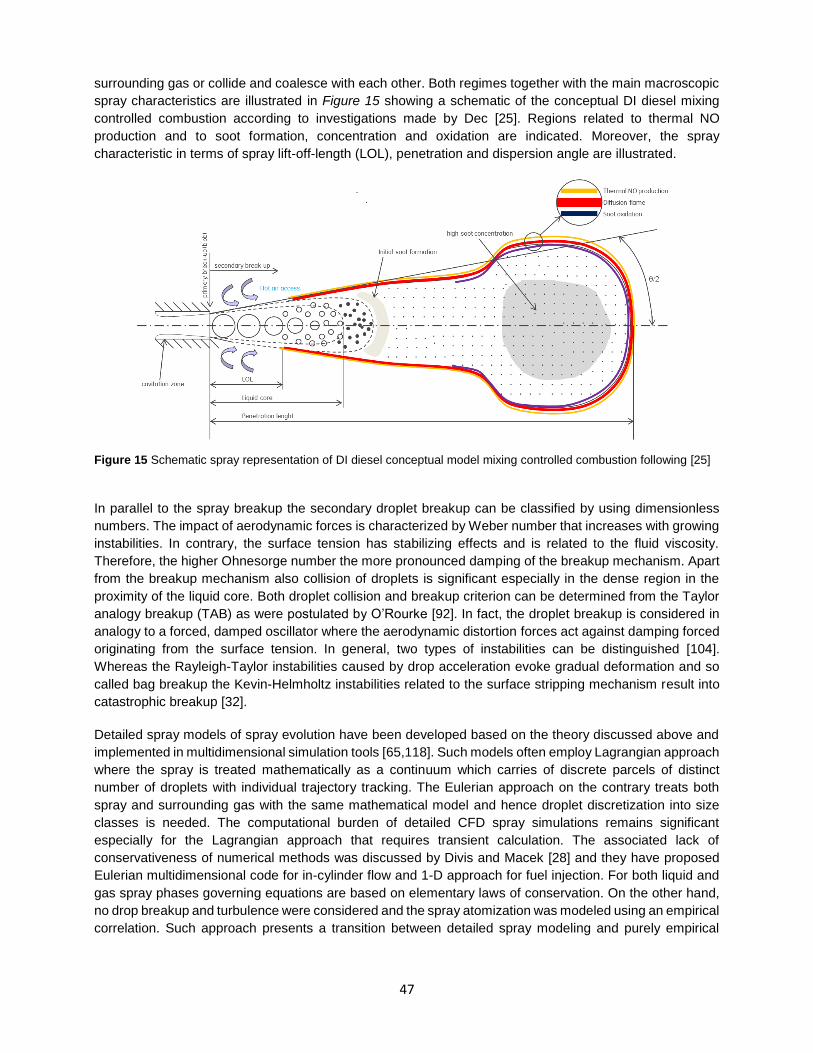
47
surrounding gas or collide and coalesce with each other. Both regimes together with the main macroscopic
spray characteristics are illustrated in Figure 15 showing a schematic of the conceptual DI diesel mixing
controlled combustion according to investigations made by Dec [25]. Regions related to thermal NO
production and to soot formation, concentration and oxidation are indicated. Moreover, the spray
characteristic in terms of spray lift-off-length (LOL), penetration and dispersion angle are illustrated.
Figure 15 Schematic spray representation of DI diesel conceptual model mixing controlled combustion following [25]
In parallel to the spray breakup the secondary droplet breakup can be classified by using dimensionless
numbers. The impact of aerodynamic forces is characterized by Weber number that increases with growing
instabilities. In contrary, the surface tension has stabilizing effects and is related to the fluid viscosity.
Therefore, the higher Ohnesorge number the more pronounced damping of the breakup mechanism. Apart
from the breakup mechanism also collision of droplets is significant especially in the dense region in the
proximity of the liquid core. Both droplet collision and breakup criterion can be determined from the Taylor
analogy breakup (TAB) as were postulated by O’Rourke [92]. In fact, the droplet breakup is considered in
analogy to a forced, damped oscillator where the aerodynamic distortion forces act against damping forced
originating from the surface tension. In general, two types of instabilities can be distinguished [104].
Whereas the Rayleigh-Taylor instabilities caused by drop acceleration evoke gradual deformation and so
called bag breakup the Kevin-Helmholtz instabilities related to the surface stripping mechanism result into
catastrophic breakup [32].
Detailed spray models of spray evolution have been developed based on the theory discussed above and
implemented in multidimensional simulation tools [65,118]. Such models often employ Lagrangian approach
where the spray is treated mathematically as a continuum which carries of discrete parcels of distinct
number of droplets with individual trajectory tracking. The Eulerian approach on the contrary treats both
spray and surrounding gas with the same mathematical model and hence droplet discretization into size
classes is needed. The computational burden of detailed CFD spray simulations remains significant
especially for the Lagrangian approach that requires transient calculation. The associated lack of
conservativeness of numerical methods was discussed by Divis and Macek [28] and they have proposed
Eulerian multidimensional code for in-cylinder flow and 1-D approach for fuel injection. For both liquid and
gas spray phases governing equations are based on elementary laws of conservation. On the other hand,
no drop breakup and turbulence were considered and the spray atomization was modeled using an empirical
correlation. Such approach presents a transition between detailed spray modeling and purely empirical

48
approaches which are employed for description of spray penetration and formation within the present model.
Therefore, a brief overview of related methods is given next.
Among important macroscopic spray parameters are the penetration length and the spray cone angle.
Numerous models were proposed at different conditions and for various fluid properties. The majority is
dated back in the past as the injection pressure levels and the state of the art injector design were way
below current standards. Hence, the applicability on present case had to be carefully assessed, including
comparison with experimental results [45]. Table 1 summarizes main correlations for the spray penetration
dependency on injection time. Based on these definitions is obvious that the spray evolution is driven mainly
by the pressure difference and density of the gas following the principle formulated in the Bernoulli equation.
Major parameters influencing the spray penetration are the nozzle hole diameter and length, gas pressure
and temperature and the injection pressure. The transition time after the injection onset from the as the
predominantly liquid spray governed phase to the phase dominated by surrounding gas entrainment is
denoted as breakup time tbr. The breakup time represents the required time for the liquid spray disintegration
into droplets. The early work done by Dent [26] does not considered these fundamental differences in spray
development before and after breakup. Varde and Popa [124] approximate spray penetration by a single
equation. However, they have considered the Reynolds number of the nozzle flow and fluid properties.
Concepts taking into account characteristics of both phases by individual correlations were developed in
[46,86]. Details related to individual approaches and applicability on the present model are discussed in the
Section 5.2.
Reference Correlation Conditions
Dent [26] 𝑠 = 3.07 (
𝑝
𝑔
)
0.25
(𝑡 𝑑0)0.5 (
294
𝑇𝑔
)
0.25
(37)
Varde, Popa
[124] 𝑠 = 1.1 𝐶10.3𝐶2
−0.008 (
𝑓
𝑔
)
0.5
(𝑙𝑛𝑜𝑧
𝑑𝑛𝑜𝑧
)0.16
𝑡0.55
𝐶1 = 𝑝 𝑓
𝑑𝑛𝑜𝑧2
𝑓2
, 𝐶2 = 𝑓
𝑑𝑛𝑜𝑧
𝑓2
(38)
pinj < 1500bar
Hiroyasu, Arai
[47] 𝑠 = 0.39 (2𝑝
𝑔
)
0.5
∙ 𝑡; 𝑡 < 𝑡𝑏𝑟
𝑠 = 2.95 (𝑝
𝑔
)
0.25
(𝑑𝑛𝑜𝑧 𝑡)0.5; 𝑡 > 𝑡𝑏𝑟
𝑡𝑏𝑟 = 28.65
𝑓𝑑𝑛𝑜𝑧
√𝑔𝑝
(39)
pinj < 400bar
Tg 295-590K
Naber, Siebers
[88] 𝑠 = 𝐶𝑣 (2𝑝
𝑔
)
0.5
∙ 𝑡; 𝑡 < 𝑡𝑏𝑟
𝑠 = (𝐶𝑣√2 𝐶𝑎
0.66 𝑡𝑎𝑛(𝜃/2))(
𝑝
𝑔
)
0.25
𝑑𝑛𝑜𝑧 𝑡; 𝑡 > 𝑡𝑏𝑟
𝑡𝑏𝑟 =√𝐶𝑎/2
𝐶𝑣0.66 𝑡𝑎𝑛(𝜃/2)
𝑑𝑛𝑜𝑧 𝑓0.5
√𝑔𝑝
(40)
pinj 750-1600bar
Tg 300-1400K
Table 1 Correlations for diesel spray tip penetration
The aerodynamic forces act on the spray entering the combustion chamber and initiate the spray breakup.
Depending on the injection pressure, geometry or cavitation the spray dispersion can be characterized by
49
the spray cone angle according the Figure 15. The air entrainment is proportional to the cone angle and
hence influences the evaporation rate and the subsequent oxidation. Depending on the measurement
position, definition of the spray contour, gas to liquid fuel density ratio and if non-evaporating or reactive
conditions were considered the individual models differ considerably. In general, the spray cone angle
depends on fuel viscosity, surface tension, injection pressure, nozzle geometry and gas density. The
pioneering work has been done by Sitkei [111].
𝜃 = 0.03 (
𝑙0𝑑0
)−0.3
(𝜌𝑔
𝜌𝑙
)−0.3
𝑅𝑒0.7 (41)
Reitz and Bracco [104] have proposed a correlation based on the aerodynamic drag induced breakup
through rise of surface instabilities according to the equation (42). In case of spray atomization, the constant
A is determined by an empirical relation as defined below.
𝑡𝑎𝑛 (
𝜃
2) =
4𝜋
𝐴(𝜌𝑔
𝜌𝑙
)0.5
𝑓 [𝜌𝑙
𝜌𝑔
(𝑅𝑒
𝑊𝑒)2
] , 𝐴 ≈ 3.0 + 𝑙0/𝑑0
3.6 (42)
Photographic spray investigations were utilized for deriving an empirical correlation for the cone angle by
Hiroyasu and Arai [47]. The initial formulation that was additionally extended by considering the diameter of
the nozzle sac hole dsac yields equation (43).
𝜃 = 83.5 (
𝑙𝑛𝑜𝑧
𝑑𝑛𝑜𝑧
)−0.22
(𝑙0
𝑑𝑠𝑎𝑐
)0.15
(𝜌𝑔
𝜌𝑙
)0.26
(43)
Naber and Siebers [88] have measured the spray dispersion angle under both nonevaporating and
evaporating conditions for a common rail injector up to 1600bar rail pressure. The evaluation of the results
acquired by the schlieren technique has shown that the evaporated spray phase is predominant at elevated
temperature. The proposed correlation (44) for the tangent of the spray half angle is valid in the region
where the spray evolution can be approximated by a gas jet behavior where the constant C is related to the
nozzle hole diameter.
𝑡𝑎𝑛 (
𝜃
2) = 𝐶 (
𝜌𝑔
𝜌𝑙
)0.19
(44)
Apart from the spray penetration and dispersion the droplet size presents an important parameter for the
evaporation and ignition process of the injected fuel. The droplet size distribution determined by the
atomization includes a broad spectrum of sizes from the large drops compared to the nozzle diameter down
to tiny droplet imminent prior to complete evaporation. To characterize the droplet size distribution average
diameter d10 and the Sauter mean diameter d32 also denoted as SMD are often used. The latter corresponds
to a droplet diameter which has an identical surface to volume ratio as the entire spectrum of considered
droplets. Several authors have investigated the droplet distribution and proposed correlation for the
averaged or SMD. Essentially, the droplet size depends on fluid viscosity and surface tension, fluid and gas
densities, injection pressure and injection nozzle geometry. Hiroyasu et al [46,47] have measured the
droplet sizes using laser diffraction analysis for fluids with various viscosity and surface tension.
𝑑32 = 0.38 𝑑0𝑅𝑒0.25𝑊𝑒−0.32 (
𝜇𝑙
𝜇𝑔
)
0.37
(𝜌𝑙
𝜌𝑔
)
−0.47
(45)

50
The length of surface waves arising from instabilities was used for droplet size calculations by Reitz and
Bracco [104]. The correlation determines the droplet at the nozzle exit and the secondary breakup effects
are not considered. Therefore, the implementation for modeling purpose is rather limited.
�̅� = 𝐶
2𝜋𝜎
𝜌𝑔𝑢2 𝑥𝑚𝑎𝑥 [
𝜌𝑙
𝜌𝑔
(𝑅𝑒
𝑊𝑒)2
] (46)
Within the correlation proposed by Wand and Lefebvre [129] mechanisms of both aerodynamic forces
causing waves on the liquid surface leading to unstable ligaments and hydrodynamic forces acting inversely
are taken in account. Therefore, so called two stage formulation for the droplet SMD was suggested and
compared with experiments on plain-jet air blasting atomizers. Further development and tuning of the
constants yield an empirical formula (47).
𝑆𝑀𝐷 = 10−3 [
√𝜎𝜌𝑙
𝜌𝑔𝑢𝑔
] (1 +1
𝐴𝐹𝑅)0.5
+ 6 ∙ 10−5 [𝜇𝑙
2
𝜎𝜌𝑔
]
0.425
(1 +1
𝐴𝐹𝑅)0.5
(47)
4.3.2 Evaporation
Spray atomization process plays a major role in the ensuing droplet heating and evaporation related to the
phase transition of the injected liquid fuel to vapor. In general, the solution of droplet heat-up and phase
transition is determined by employing energy and mass conservation laws. Numerous models were
established for simulation phenomena related to droplet heating and evaporation ranging from relatively
simple tools to models considering complex physics such as effects of temperature gradient inside droplets,
inner flow recirculation or radiative heating. Total vapor mass flux coming from the spray jet depends on the
numbers of droplets and their size distribution. Exact determination of droplets size distribution is not
feasible even with detailed multidimensional models and hence equivalent droplet size in terms of SMD is
employed. Subsequently the number of droplets can be calculated for each time step and the evaporation
model defines the instantaneous droplet mass reduction rate.
The D2-law assumes an isolated, single component fuel droplet oxidized in a quiescent environment and
relates the droplet diameter reduction linearly to the time progress. The applicability is suitable for simplified
models only since an infinite thermal conductivity is assumed and hence droplet temperature remains
constant. However, the droplet evaporation in a high temperature environment does not follow the D2-law
but consist of rapid heating and stationary evaporation phases. More detailed hydrodynamic models of
droplet evaporation consider fuel vapor diffusion from the droplet surface to the ambient gas and the effect
of convection into the surrounding gas.
For the present application, a significant simplification has been made assuming spherical and symmetrical
single-phase droplets with constant density and pressure and neglecting the impact of radiation, semi-
transparency of droplets, vapor superheating and impact of chemical reactions. Hence, the main driver of
the droplet heating and evaporation is attributed to both diffusion and convection. Adopting the classical
Spalding hydrodynamic model concept [115], the rate of droplet evaporation is determined by relation (48)
where the fuel density f and diffusion coefficient Df are related to the fuel vapor, rdr represents the
instantaneous droplet diameter initiated by Sauter mean diameter (SMD), determined by means of a
correlation proposed by Varde [124]. Sh denotes Sherwood number and BM Spalding mass transfer
number.

51
𝑑𝑚𝑑𝑟
𝑑𝑡= 2𝜋 𝐷𝑓 𝑓
𝑟𝑑𝑟 𝑆ℎ 𝐵𝑀 (48)
Sherwood number can be expressed in a form defined by equation (49) with Sh0=2 for non-evaporating
droplets. BM denotes Spalding mass transfer number depending on the mass fractions of the fuel vapor at
the droplet vicinity and in the free stream conditions.
𝑆ℎ = 𝑆ℎ0
ln(1 + 𝐵𝑀)
𝐵𝑀
(49)
Based on the change of the droplet mass transfer rate given by the equation (48) the droplet diameter can
be determined according to Faeth [33] as shown below.
𝑑𝑟𝑑𝑟
𝑑𝑡=
1
4𝜋 𝑟𝑑𝑟2𝜌𝑓
𝑑𝑚𝑑𝑟
𝑑𝑡−
𝑟𝑑𝑟
3𝜌𝑓
𝑑𝜌𝑓
𝑑𝑡 (50)
The hydrodynamic model assumes the vaporization rate is largely given by the rate of diffusion which is not
valid in the early stage of vaporization process as the droplets temperature is low compared to the ambient
gas conditions. The droplet temperature is derived from the energy balance taking into accounts the effect
of convective heat transfer between the droplet and ambient gas and latent heat of vaporation L by equation
(51) according to [33]
𝑑𝑇𝑑𝑟
𝑑𝑡=
1
𝑐𝑑𝑟
(3
𝑓𝑟𝑑𝑟
(𝑇𝑔 − 𝑇𝑑𝑟)𝑁𝑢 −𝑑𝑚𝑑𝑟
𝑑𝑡𝐿 (𝑇𝑑𝑟)) (51)
4.3.3 Ignition
The ignition process of diesel fuel is determined by many factors including the fuel composition, spray
formation, mixing with oxidizer, initial thermodynamic conditions and the actual chemistry. Specifically, it is
a function of properties such as cetane number, viscosity, nozzle hole size, injected quantity or injection
pressure. In general, the ignition delay can be characterized as the time necessary for visible fire to appear
in the pre-mixed zone of spray since the fuel injection onset. Not only combustion controllability but also
engine efficiency, emissions and combustion noise are strongly impacted by the ignition process. The
ignition delay can be divided into two major parts comprising physical and chemical ignition delays. The
physical ignition delay is required for spray atomization, evaporation and mixing with the oxidizer whereas
the chemical process comprises a complex mechanism characterized by several reaction regimes.
Depending on the thermal and hydrocarbons chain-branching effects three regimes can be distinguished,
namely high, medium- and low-temperature regimes [79]. Except for the thermal dependency the reactions
within the ignition delay period are also pressure dependent in high and medium temperature regimes. The
low temperature regime includes both chain branching and addition reaction and the pressure effect is
eliminated. Figure 16 shows calculated ignition delay curves for n-heptane diesel surrogates at various
pressure levels with solid curves representing reduced mechanism and single points experimental data.

52
Figure 16 n-heptane/air ignition delay at stoichiometric conditions [103]
The complexity of preflame reaction depending on ambient condition, concentrations or type of fuel requires
solution of detailed chemistry for generic validity. However, such approach is out of the scope of the present
study. Moreover, detailed kinetics are not prerequisite to reach reliable ignition delay predictions for diesel
fuel. Typically, the ignition ig delay can be roughly approximated by a single formula for an assumed bulk
single stage reaction in a form of an Arrhenius approach (52) where cylinder pressure and temperature as
well as activation energy Eact and model constants are taken in account.
𝜏𝑖𝑔 = 𝐶𝑝𝑐𝑦𝑙
−𝑛 𝑒(
𝐸𝑅 𝑇𝑐𝑦𝑙
)
(52)
A brief overview of selected ignition delay correlations for DI diesel combustion are summarized in Table 2
below in form of the main parameters that appear in the general expression for the ignition delay.
Reference Fuel C n Eact
Wolfer [135] (1938) Diesel, CN>50 0.44 1.19 4650
Stringer [117] (1969) Diesel, CN=49 0.0409 0.757 5473
Kadota [58] (1976) n-dodecane 6.58 0.52 4400
Watson [131] (1980) Diesel 3.45 1.02 2100
Hiroyasu [48] (1983) Diesel 0.01 -1.04 2.5 6000
Assanis et al. [4] (2003) Diesel 2.4 -0.2 1.02 2100
Table 2 Ignition delay correlations for DI diesel combustion
The ignition delay is commonly defined as a time elapsed between the start of injection (SOI) and start of
combustion (SOC). The definition of SOI is typically assigned to the initial lift of the injector needle. On the
other hand, several methods relying on diverse principles are known for SOC determination. Whereas the
optical investigations in constant volume vessels or RCM utilize methods linked to OH or CH radicals
formation detected by chemiluminescence the full scale engine test without optically accessible combustion
chamber rely on detection of sudden change in second derivative of cylinder pressure history or HRR onset
criterion. Numerous experiments have been carried out to investigate ignition delay of a diesel fuel. Many
of them, however, were performed at ideal conditions in constant volume vessels or rapid compression
machines not considering the relevant engine operation boundaries such as turbulent flow field or
53
pronounced temperature nonuniformity. For instance, Wolfer has proposed a correlation based on
experimental results in a constant volume vessel. Kadota [58] has suggested a similar approach which was
further developed together with Hiroyasu by introducing an additional dependency on the equivalence ratio.
Stringer et al. [117] have investigated various hydrocarbon of fuels while injecting them into a steady air
stream at conditions up to 60bar pressure and 980K temperature. Under real engine conditions the spatial
differences as well as the flow field and turbulence contribute substantially to spatial uniformity deviations
and hence influence the ignition delay to a certain extent. On the contrary, engine based correlations are
not always accurate enough since predictions contain uncertainty related to SOI and SOC determination.
Assanis et al. [57] have assessed various correlations and employed the approach for ignition delay period
in a heavy-duty turbocharged DI diesel engine. In addition to the basic correlation a dependency on
equivalence ratio was introduced and validated against both steady state and transient experiments.
4.4 Dual Fuel Combustion
Combustion of multiple fuel extends the flexibility and applicability of reciprocating engines significantly. On
the other hand, specific changes have to be done in terms of engine layout which partially constrain
individual operation modes. For a dual fuel operation based on a diesel engine and being capable to burn
gaseous fuels two main concept. First, fumigation of relatively small amount of gas is introduced into to
intake manifold of a standard diesel engine. This approach does not offer significant fuel economy
improvements or emission reduction and can be justified mainly due to differentiation for diesel and gas fuel
prizes. The second approach requires modification of the engine design since merely a fraction of diesel
fuel is injected in order to ignite the lean gaseous mixture. These modifications are necessary since the
mainly premixed combustion concept corresponds to the Otto principle limited by knock phenomena. Before
attaining such result for a new dual fuel concept for large low speed 2-stroke engines the complexity of the
dual fuel combustion process has to well understood.
Depending on the method of introducing the gaseous fuel into the engine several concepts can be
distinguished. In the past, applications with gas introducing upstream the turbocharger, inlet port admission
or direct in-cylinder concepts were investigated and brought to a product. Recently, low pressure port
admission of the gaseous fuel is referred as the state of the art for medium speed 4-stroke engines.
Nevertheless, such concept would not be viable for the large 2-stroke engine concept due to a common
piston underside volume and related safety issues. Thus, direct gas admission has been assessed as the
optimal concept in terms of combustion, emissions and safety aspects. In order to ignite lean and stratified
gas mixtures with the oxidizer a strong ignition source is needed securing a repeatable ignition of the large
combustion chamber volume. This becomes an additional challenge in respect of low compression
temperatures resulting from the reduced compression ratio. Direct pilot injection with a double needle
injector has proven to be a reliable solution for medium-speed DF 4-stroke engines since it provides
repeatable ignition sufficient combustion stability at a minimum diesel fuel quantity. However, for 2-stroke
DF engines a concept with a pilot combustion chamber (PCC) was developed due to reasons discussed
above. The working principle of large DF engine with a direct low pressure gas admission and diesel pilot
ignition is illustrated in Figure 17. Hot conditions in the pre-chamber and concentrated energy of the pilot
fuel result into minimized ignition delay and eliminate stochastic variations effective SOC due to dilution. In
order to generate rapid pressure rise in the PCC and induce a powerful pilot flame impulse penetrating well
into the main combustion chamber, the injection duration is being kept short as possible. In this way, the
PCC concept provides ignition energy well distributed in the combustion chamber at energetic pilot fuel
quantities of below 1% of at full load operation and a stable DF combustion can be achieved throughout the

54
entire operating range. Each cylinder is equipped by two PCC featuring single pilot injector and the fuel is
supplied by a down-sized common rail system and high pressure fuel pump.
Figure 17 Lean burn concept for large 2-stoke DF engines [91]
Lean burn technology for a large 2-stroke marine engine presents significant advantage in terms of raw
engine emission compared to a state of the art diesel engine as already shown in Figure 3. Premixing of
gaseous fuel with oxidizer during the scavenging phase leads to overall lean mixture so that the peak
combustion temperature level can be reduced substantially. Hence, the major benefit of a lean burn concept
employing natural gas as a main fuel in terms of nitrogen oxides reduction is evident. Together with nearly
zero sulfur-oxides emissions and particulates cut to a minimum the premixed gas combustion becomes
highly attractive since the employment of a costly aftertreatment system can be omitted. Furthermore, the
low C/H ratio in comparison to other hydrocarbons as well as the chemical equilibrium properties of involved
reactants and products allow optimizing carbon dioxide emissions and improvement of thermal efficiency,
respectively. Hereby, a comparable efficiency to a high compression ratio Diesel engine can be achieved.
Despite of the incomplete burnout of the introduced fuel characteristic for a premixed lean burn concept,
unburned hydrocarbons are cut down to a minimum by an appropriate choice of ignition source and adjusting
the exhaust valve timing. Therefore, the methane slip remains uncritical way below the engineering targets.
On the other hand, the stochastic character of the premixed combustion with its sensitivity to the mixture
homogeneity and instabilities due to gas composition variations has to be assessed carefully. Improper
selection of engine settings may lead to knock or extensive methane-slip. Moreover, in case of a large
uniflow scavenged 2-stroke engine the low rotational speed, direct injection of the lubricating oil on liner
walls or into the piston ring pack and inevitable interactions between the fresh fuel-oxidizer mixture and hot
burned gases from the previous cycle need to be considered. Determined by 2-stroke engine cycle
constrains, the admission of the gaseous fuel is required to take place coincidently with the scavenging
process. Therefore, special attention has to be paid to the elimination of non-uniform reactant mixtures and
charge stratification stimulation. Further, a stable pilot jet penetrating into the combustion chamber is
prerequisite for repeatable ignition onset of the main fuel and overall engine controllability, especially at low
load and idle operating conditions.

55
4.4.1 Laminar Premixed Flames
Deflagration of an un-stretched flame through a quiescent premixed fuel-oxidizer environment is determined
by its laminar speed. The flame propagation is essentially controlled by the fuel consumption and depletion
of radicals within the reaction zone inseparably related to thermal and molecular diffusion processes.
Laminar flame velocity is an important property of a flammable mixture depending on fuel properties and
thermodynamic state. It contains essential information related to the mixture reactivity and exothermicity.
Detailed knowledge of the laminar flame propagation provides insights into combustion characteristics as
heat release rate, quenching or emission formation. Furthermore, the laminar flame velocity is indispensable
for modeling the turbulent flame propagation. Hence, a fundamental overview of the laminar flame
characteristics is essential in capturing the complexity of the turbulent premixed combustion. Figure 18
illustrates the reaction zone of an unstretched laminar flame characterized by temperature and
concentrations gradients.
Figure 18 Schematics of laminar flame for methane following the asymptotic flamelet theory, Peters [97]
In this schematic of the asymptotic flame analysis the fuel and oxidizer are transported from the chemically
inert preheat zone l by the laminar flame velocity SL and diffuse into the reaction zone stands for the
reaction zone thickness alternatively labeled as thin inner layer. The reaction zone thickness for methane
flames in air typically ranges between 10-100μm in order of magnitude. As soon as the mixture reaches the
inner layer temperature T0 due to heat conduction, radical production and oxidation start to take place.
During this phase fuel is being consumed. Within the stagnation point of the inner flame structure, the
gradient of H radicals towards the burnt gas zone increases substantially, such that production of H2 by
chain-branching reactions can no longer balance the losses. Further rise in temperature completes the
entire depletion of radicals as well as H2 and CO in hydrocarbon flames within the oxidation layer . The
processes taking place in the oxidation layer are assumed to be at equilibrium whereas at the boundary to

56
the reaction zone an intermediate non-equilibrium layer can be detected [97]. The thickness of individual
zones corresponds to the following order < l.
Such a representation is based on a flamelet concept theory where the combustion occurs in thin layer
embedded within the flow field. The interaction between flamelets and the main flow field is significant. For
the most applications referring to reciprocating engines or gas turbines the thin reaction zone the fuel
oxidation can be described by the flamelet concept. Specific conditions at which the thin reaction zone
acquires prominence necessitate that the flame thickness becomes smaller than the smallest turbulent
length scale corresponding to the Kolmogorov scale. In parallel the dominance of the turbulent intensity over
the laminar flame velocity causes interactions between the flow field and the flame front that corrugates the
front [97]. Detailed classification derived from the turbulent conditions will be discussed in the following
section.
The premixed combustion is characterized by hundreds of elementary reactions. Comprehensive
computations of a laminar flame taking into account the full complexity have been made by Warnatz [130].
Simplifying assumptions related to single-phase flow, low Mach number and negligible radiative heat
transfer are needed to describe the chemistry in a reduced form. As mentioned previously, laminar flame
propagation is driven by temperature and concentration gradients governing thermodiffusive and
hydrodynamics effects. The laminar flame velocity is defined based on propagation of the flame front as the
unburned gas moves into the reaction zone and is normal to the flame front relatively to the unburnt mixture.
The magnitude of the laminar flame velocity is influenced by fuel properties, concentrations as well as
temperature and pressure conditions. Excluding thermodiffusive instabilities when Le approaches unity
implying constant and uniform flame enthalpy allows to solve thermochemistry by means of the transport
equation of a single progress variable. Adopting the thermosdiffusive theory of Zeldovich and Semenov
[143], the laminar flame velocity yields relation (53) proportional to the mass diffusivity D and laminar mixture
characteristic time scale that can be approximated by the reaction zone thickness .
𝑆𝐿~(
𝐷
)1/2
~(𝐷
𝛿𝐿
)1/2
(53)
For the Le=1 the mass diffusivity is equal to the thermal diffusivity and depends on the mixture properties
according to (54) where u is the density of unburned zone.
𝐷 =
𝑏
𝜌𝑢𝑐𝑝
(54)
Assuming minor thermal impact of reaction rates in the preheat zone, the reaction in the thin inner layer
takes place at the combustion temperature and the convective term can be neglected [143]. Then the
characteristic time for lean mixtures where << 1 is given by equation (55) where E denotes activation
energy and C is an adjustable frequency constant. In this respect, the characteristic time is not only
determined not but the chemistry but also by the flame structure.
𝜏 =
𝜌𝑢 𝑍𝑒2
2𝐶𝜌𝑏2 𝐹𝑌𝑂2
𝑀𝑂2
𝑒(
𝐸𝑅 𝑇𝑏
) (55)
Ze defines the Zeldovich number in terms of dimensionless activation energy of the flame velocity. In other
words, it describes the dependency of the reaction rates rapidity on the temperature that can be also

57
interpreted as a relation of the thickness of the flame front conductive region to the effective thickness of
the reaction zone.
𝑍𝑒 =
𝐸(𝑇𝑏 − 𝑇𝑢 )
𝑅𝑇𝑏2 (56)
Various definitions for the flame thickness can be found in the literature. Whereas some authors define the
flame thickness from the inner layer temperature T0 to the combustion temperature T, e.g. adiabatic flame
temperature, other determine it as a distance between intersections of the temperature profile and its
tangent [97]. Combining equations (53) and (54) yields a general expression for the laminar flame thickness:
𝛿𝐿 =
𝑏
𝜌𝑢𝑐𝑝𝑆𝐿
(57)
Since the reaction zone is presumed to be very thin the laminar flame thickness corresponds primarily to
the preheat zone of the flame structure in Figure 18. Furthermore, it characterizes the flame quenching
distance as the flame extinguishes in the proximity of a cold wall. Laminar flame thickness decreases with
increasing pressure as a consequence of reduced diffusivity. This effect leads to flame velocity decrease
due to the impact of the molecular diffusion on flame front propagation [29]. High unburned zone
temperature also causes reduction of the flame thickness but the elevated diffusivity accelerates the laminar
flame velocity. Similarly, the richer the mixture the higher reactivity results in thinner flame thickness. These
effects are directly connected to flame front instability and cellularity sensitivity as discussed in following.
In addition to the thermal theories postulated in late 19th century the importance of the molecular diffusion
is emphasized [29]. Solving conservation equations considering both thermal and molecular diffusion result
into a general formula (58) for the laminar flame velocity where the initial conditions denoted by zero
correspond to the reaction zone state as shown in Figure 18 and T is assigned to the final temperature of
combustion. The relatively simple expression for relation is deduced from the fact that within the flame
reaction zone the rapid rise in chemical reaction rate occurs at temperature close to the combustion
temperature corresponding to adiabatic flame temperature. Thus, the integral below the square root
approximating the expended heat is rather insignificant and the majority of the reaction heat originates from
the thermal conductivity. The initial influence of the thermal conductivity is not in the contradiction with the
progress of chemical chain reactions driven by the equilibrium properties of the reactants or increase
exponentially with the time [29]. In fact, the reaction zone thickness is substantially thinner than the
preheating zone so it can be postulated that the temperature window where the bulk reactions take place is
rather narrow.
𝑆𝐿 =1
𝜌0𝐻√2∫ �̇�𝑑𝑇
𝑇
𝑇0
(58)
With respect to a basic experimental measurement of the laminar flame velocity assuming spherical
deflagration outwards from the central ignition location and neglecting burn gas expansion, flame front
curvature and strain the laminar flame velocity is given by (59) for L / rfl <<1. Note that the time derivative
of the flame radius stands for experimentally flame speed directly measured. In the present work SL stands
for stretched laminar flame velocity in the sense of burning velocity.
𝑆𝐿 =
𝜌𝑏
𝜌𝑢
𝑑𝑟𝑓𝑙
𝑑𝑡
(59)

58
Determination of laminar flame velocity at thermodynamic conditions typical for unburned mixture in
reciprocating engines is essential to the subsequent solving of turbulent flame propagation directly impacting
the resulting heat release rate. There are several competing methodologies which can be employed for
executing the laminar flame velocity measurements. Although numerous experimental investigations and
computational studies have been undertaken on the laminar flame velocity investigation [16,38,44,76,94,
122,123,134] they capture the flame propagation mainly at ambient conditions (p=1bar, T=298K). Table 3
summarizes the experimental investigations of laminar flame velocity for methane and NG air mixtures from
various authors including the information related to validity range and applied methodology.
Table 3 Overview of experimental investigations of laminar flame velocity for methane- and NG-air mixtures
Experimental results for laminar flame velocity at normal temperature over equivalence ratio sweep are
plotted on Figure 19. Except for the maximum peak at slightly rich conditions the dependency on the initial
pressure is also shown completed by computational results of GRI-Mech 3.0 detailed mechanism.
Figure 19 Laminar flame velocity experimental results as function of equivalence ratio for CH4/air mixture at 1, 5 and
10bar and 300K ambient conditions. GRI-Mech calculation is represented by solid lines. Merely very limited data are available for engine relevant conditions due to difficulties arising from flame
instabilities that can be related to hydrodynamic and thermodiffusive effects. Indeed, the major challenge to
perform measurements at such conditions is to ensure flame stabilization through minimizing the stretch
and curvature effects. The flame unsteadiness complicates experimental capturing of laminar flame
Reference fuel p [bar], T [K], Methodology
Tseng et al. [122] CH4/air 1, 298, 0.6-1.35 const. vol. chamber, shadowgraphy
Vagapoulos, Egolfopoulos [123]
CH/air 1, 298, 0.7-1.4 vertical burner w/ stagnation plane, LDV
Gu et al. [38] CH/air 0.1-10, 300-400,0.8-1.2 const. vol. chamber, schlieren
Hassan et al. [44] 0.5-4,298,0.6-135 const. vol. chamber, shadowgraphy
Rozeachan et al. [106] CH4/air 1-60, 298, 0.6-1.4 const. vol. chamber, schlieren
Liao et al. [76] NG 0.5-1.5,300-400,0.6-1.4 const. vol. chamber, schlieren
Ogami, Kobayashi [94] CH4/air 1-10, 298-600,0.8-1.3 slot nozzle burner, PTV & OH-PLIF

59
propagation. In fact, for lean mixtures at elevated pressure and temperature the impact of flame stretch and
distortion of the surface area do not concede the existence of laminar flame front. Since at such conditions
the combustion progress is governed by the turbulent burning velocity the related laminar flame velocity has
to be often extrapolated or determined using reaction kinetics.
A comprehensive classification of individual measurement techniques was presented by Andrews and
Bradley [2] dividing them into constant pressure and constant volume categories and proved the need for
considering the flame thickness when evaluating experimental results. The first category is represented by
slot or Bunsen type burners where the kinematic balance of the gas flow and the flame angle yields the
laminar flame velocity. The relatively simple experimental setup is on the other hand linked to a low accuracy
and limited initial conditions. Measurement in spherical vessel at constant volume enable unconstrained
even flame propagation radially from the vessel center. For a proper interpretation of experimental results,
the pressure changes and instabilities due to curvature in the flame front have to be taken into account. As
long as the burn volume relative to the total volume of the vessel stays small the impact of the pressure
change can be neglected. Hence, this approach provides more realistic results in regard of typical conditions
occurring in reciprocating engines. The procedure to extract the laminar flame velocity is based on the flame
displacement with respect to the unburned mixture and the ratio of unburned to burned gas densities. Lately,
the demand for measurements at the limit of flammability and at elevated pressure and temperature has
become stronger. Therefore, sophisticated measurement setup and data acquisition techniques need to be
applied such as wall stagnation flame configuration or particle image velocimetry (PV). For preheated gases
at high pressures the opposed and wall stagnation flow configurations are more favorable since providing
nominally steady flame conditions [62]. In case of the opposed flame configuration, the effect of heat losses
on the flame propagation can be eliminated but a significant strain rate cannot be neglected. Therefore, the
results need to be corrected accordingly.
Results of experimental investigations are often taken as a basis for developing computational correlations
for the laminar flame velocity. In early eighties Metghalchi and Keck [83] have investigated flame
propagation of iso-octane at elevated pressure using extrapolation from low pressure results. They have
developed an empirical correlation for the laminar flame speed dependent on temperature, pressure, dilution
of inert gas and equivalence ratio of the mixture where Tu,ref = 298K, pref = 1bar. However, the generic
employment of the polynomial expression is not feasible due to negative flame velocities for high and low
equivalence ratios.
𝑆𝐿 = 𝑆𝐿,𝑟𝑒𝑓 (
𝑇𝑢
𝑇𝑢,𝑟𝑒𝑓
)
𝑓1
(𝑝
𝑝𝑟𝑒𝑓
)
𝑓2
(1 − 2.1 𝑌𝑑𝑖𝑙)
𝑆𝐿,𝑟𝑒𝑓 = 36.92 − 140.51( − 𝑀)2
𝑓1 = 2.18 − 0.8( − 1)
𝑓2 = −0.16 + 0.22( − 1)
(60)
An alternative empirical approach was outlined by Gülder [39] in an exponential form that approximates the
rich and lean limit conditions partially better. However, the differences between both cases cannot be fitted
accurately due to the symmetrical character of the applied exponential function as presented below.
𝑆𝐿 = 42.20.15𝑒−5.18(−1.075)2 (61)

60
Correlations for both methane and natural gas flames were determined by Liao et al [76] from schlieren
photography and corrected for the flame stretch rate. In addition, dilution of the combustible mixture was
implemented in the form of a polynomial function. The level of initial temperature was 300-400K and the
maximum pressure at 1.5bar. Nevertheless, especially at higher equivalence ratios the fit does not show a
good agreement with the experimental data for neither methane nor natural gas cases. Laminar flame
velocities at minimum strain rate were further investigated by laser Doppler velocimetry on a vertical burner
opposed by a stagnation plane for atmospheric pressures and range of equivalence ratios [123]. Striving for
near-zero stretch rate, the velocities were determined at the transition onset from the planar flame. However,
this was reported to be challenging for lean mixtures at Le < 1 as instabilities start to grow. Ogami and
Kobayashi [94] investigated flame velocities of methane-air mixture in a high pressure chamber by particle
tracking velocimetry and laser induced fluorescence for OH-radicals tracking for conditions up to 600K and
10bar. The instability onset at high pressure levels was suppressed by helium dilution.
Bradley et al. [17] published a computational study with the focus to the flame stretch impact on the
associated burning velocity for a case of spherical methane-air flame propagation using a reduced reaction
scheme. The Markstein length was calculated to express the influence of both flame curvature and flow field
strain individually. Another numerical study related to laminar velocity and flame thickness was done by Witt
and Griebel [134] for temperatures and pressures up to 823K and 30bar, respectively and GRI3.0-Mech
reaction mechanism [114] was claimed to provide the best agreement with the experimental data taken from
literature. The mechanism comprises of 325 reaction taking into account 53 individual species. Validation
has been done against a number of surrogate fuels with varying hydrogen/carbon ratio. The performance
of the mechanism was compared with data from a flow reactor for temperatures 500 – 1000K and pressure
of 12.5bar. Additionally, the validity was proven using test data from RCM at temperature window 645-715K
and pressures up to 20bar. In addition to the GRI-Mech numerous mechanisms were applied to the
calculation of laminar flame velocity and ingnition delay for methane and natural gas. Recently, a
comprehensive overview of detailed kinetic mechanisms was summarized by Reitz et al. [103]. As plotted
in Figure 20, besides the GRI-Mech also the NUI mechanism was identified to perform well for methane air
mixture oxidation especially at intermediate temperature conditions and under elevated pressure relevant
for operation of reciprocating engines
Figure 20 Overview of Laminar flame velocity at ambient conditions over equivalence ratio calculated by various
detailed mechanisms [103]

61
As stated in connection with measurement techniques, freely propagating laminar premixed flames are by
the nature exposed to instabilities related to finite flame thickness, stretch and unsteadiness. There are two
major sources of these flame instabilities having origin in hydrodynamic and thermodiffusive effects [38]. In
general, effects related to molecular diffusion are dominant and can either increase or reduce the instabilities
arising from hydrodynamic ones. The hydrodynamic instability results from thermal expansion. Especially
for large scale flame it becomes dominant causing creases in the flame front leading to wrinkling. Such
flame structure has been experimentally observed on the surface of expanding flames [109]. On the other
hand, thermodiffusive effects have in general stabilizing impact and are dependent on the relative diffusion
of species and heat into the flame zone. This process is characterized by Lewis number Le (62) representing
a ratio of thermal to mass diffusivity assuming Fick’s law for the diffusion flux as well as identical temperature
and equal diffusivities for all species.
𝐿𝑒 =
𝑎
𝐷=
𝜌𝑐𝑝𝐷=
𝑆𝑐
𝑃𝑟 (62)
Positive flame curvature when Le>1 leads to flame front deceleration due to increased cooling effect
whereas at Le>1 the negative flame curvature causes apparent concentration rise, which in turn increases
the laminar flame velocity due to elevated temperature in the reaction zone. It has been also shown that
Lewis number exceeding unity and heat losses promote flame extinction but variation in density has an
inverse effect [97]. Interaction between hydrodynamic and thermodiffusive instabilities initiate flame cracking
due to oscillations and give rise to a cellular flame character. Due to enhanced flame front area, cellularity
accelerates the flame propagation as the cells start to grow and recombine. Following suggestions of several
researches, this might be considered as a source of turbulence directly generated by the flame progress.
Already early experimental investigations of the Bunsen flame cone have proven differences of the flame
velocity in vicinity of the flame cone tip. These differences are caused by the strong curvature that results
into increased preheating of the unburned zone by the lateral flame zone. Consequently, the spatial nature
of flame within a flow field causes flame stretch that has a direct impact on the flame speed. The total stretch
rate is defined as proportion of a planar element and its time derivative.
=
1
𝐴 𝑑𝐴
𝑑𝑡=
1
𝑟𝑓𝑙
𝑑𝑟
𝑑𝑡 (63)
In order to determine the stretch rate Abdel-Gayed and Bradley [1] proposed to introduce Karlovitz flame
stretch factor K incorporating the turbulence influence on the laminar flame characteristic
𝐾 =
𝛿𝐿
𝑆𝐿
=𝛿𝐿
𝑆𝐿
𝑢′
𝑙𝑇 (64)
Following the theory of Markstein, the tendency to instabilities due to transport processes is characterized
by Markstein length LM representing the measure of response of the flame stretch as follows
𝐿𝑀 = 𝛿𝐿𝑀𝑎 (65)
where Ma is the Markstein number essentially dependent on Lewis number Le, activation temperature for
kinetics and adiabatic flame temperature. For positive Ma values the flame stretch reduces the burning
velocity of methane in the air. Quantifying the effect of flame stretch is essential to gain better understanding

62
of the flame acceleration and quenching since the effect of stretch also impacts the turbulent premixed
flames in the thin reaction zone regime. This can be related to the interactions between diffusive processes
and the deformation of the flame front by turbulence [122]. Adopting the definition of the flame stretch and
at the same neglecting the differentiation between strain and curvature based contributions to the stretch,
the resulting stretched laminar flame velocity is given by equation (66).
𝑆𝐿, = 𝑆𝐿 − 𝐿𝑀 (66)
In dependency on equivalence ratio and the actual gas composition at sufficiently high stretch rates the
flame is extinguished. Substitution for the Markstein length and the flame stretch by equations (63) and (64)
respectively, the relationship (66) yields in an algebraic expression for the stretched laminar flame speed
(67) as a function of Markstein number, laminar flame characteristic and turbulence properties that are
directly related to the engine operation and associated in-cylinder thermodynamics.
𝑆𝐿, = 𝑆𝐿 (1 − 𝑀𝑎
𝛿𝐿
𝑆𝐿
𝑢′
𝑙𝑇) (67)
It is obvious that the laminar flame velocity is not determined only based on thermodynamic state for a given
gas composition but there are numerous effects related to the local conditions impacting or arising from the
thermodiffusive processes within the flame front. Several important parameters can be identified in this
respect that play a fundamental role in the laminar flame velocity propagation and thus shape the associated
oxidation process. They can be assigned to unstretched laminar flame velocity, Markstein number and
extinction stretch rates [16]. It is concluded that high pressure and temperature promote flame extinction
and instabilities especially at very lean or rich conditions. Such behavior is of particular interest and has to
be assessed carefully when defining computational models.
4.4.2 Turbulent Premixed Flame
Fundamentals of turbulent flow were discussed in Section 4.2. Caused by the turbulence impact, the
premixed flame front propagates at a speed that is not only a function of the mixture related chemical and
transport properties but also a function of the flow and turbulent intensity. Thus, the impact of turbulence
changes the premixed flame front propagation and transforms its initial laminar structure substantially.
Nevertheless, quantification of turbulent effects on the transport properties within the reaction zone is not
as definite as for the laminar case due to high complexity and randomness. In order to describe interactions
between the turbulent flow field and the flame front characteristic dimensionless numbers are defined.
Parallel to the definition of Reynolds number (24) the turbulence level is characterized by the turbulent
Reynolds number ReT as a ratio of the turbulence intensity, integral legth scale and the fluid viscosity (68).
At high ReT the flame is destabilized by momentum forces exceeding the viscous forces and becomes highly
unsteady.
𝑅𝑒𝑇 =
𝑢′𝑙𝐼𝜈
=𝑙𝐼𝛿𝐿
𝑢′
𝑆𝐿
(68)
Damköhler number Da (68) presents the ratio of the turbulent mixing time scale 𝑙𝐼/𝑢′ linked to the largerst
eddies impacting the stretch and wrinkle of the flame front to the chemical scale 𝛿𝐿/𝑆𝐿 essentially
representing the duration of the chemical reaction. Large values of Damköhler number characterize

63
combustion regimes determined by the mixing processes and result in a distinct sheet type flame front. On
the other hand, Da values below unity stand for oxidation with intense mixing governed by chemical kinetics.
𝐷𝑎 =
𝑙𝐼 ∙ 𝑆𝐿
𝑢′ ∙ 𝛿𝐿
=𝑙𝐼𝛿𝐿
(𝑢′
𝑆𝐿
)
−1
(69)
Another characteristic in terms of flame strech and wrinkle is defined by Karlovitz number Ka and is directly
linked to the Karlovitz stretch factor K determined by (64). It relates to the smallest Kolmogorov scales and
the characteristic chemical time according to the relation (70).
𝐾𝑎 = (
𝑙𝐼𝛿)−1/2
(𝑢′
𝑆𝐿
)
−3/2
= (𝛿
𝑙𝐾)2
(70)
Differences turbulent conditions defined by the characteristic number defined above give rise to qualitatively
various regimes of premixed combustion distinguished by specific processes occurring in the reaction zone
and the vicinity such as the rapid fluctuations of the flame front with pronounced wrinkling and vorticity.
These factors lead to enhancement of thermodiffusive effects characterized by Lewis number Le so the
oxidation process is being affected by the flame structure and vice versa. While increasing the turbulent
intensity the flame front becomes wrinkled. Due to effects caused by transport properties within the turbulent
flame zone the wrinkled flame may transform into corrugated condition and finally into broken reaction
zones. The individual regimes of turbulent premixed flames can be classified by the use of characteristic
numbers into several groups.
A general approach for classifying turbulent flame regimes by means of relating them to the ratio of
characteristic velocities u’/SL over the ratio of characteristic length scales lI/L was postulated by Borghi [10]
and further extended by Peters [97] as shown on Figure 21. The region for ReT<1 is characterized by low
turbulence level and laminar flame propagation. Moving in the counter clock-wise direction below the line of
u’/SL equal to unity the extreme cases with large eddies and domination of laminar flame speed over the
turbulence intensity are typical for the wrinkled flame regime. In this phase the flame thickness is smaller
than the Kolmogorov scale and thus the flame propagation is barely affected by turbulence. For application
in combustors this regime is not of practical interest.
Above the line of constant u’/SL ratio the corrugated flamelets regimes with more intense flame front
wrinkling is located. It is characterized with ReT >1 and Ka < 1, i.e. the flame thickness is smaller than the
size of the Kolmogorov scale. Therefore, the reactive flame structure is embedded within the smallest eddies
and the propagation of the flame front becomes quasi-laminar since the turbulence does not disrupt the
flame structure significantly.
The border line separating the corrugated flamelets regime from the thin reaction zones regime is given by
the Ka = 1 which indicates that the flame thickness is equal to the Kolmogorov length scale also known as
Klimov-Williams criterion. Due to the more intensive turbulence the flame wrinkling increases which leads
to an enhanced flame front area resulting to accelerating the global burn rate. In this regime, the intensified
heat and mass transport dominate the local quenching effects. However, since the reaction zone is not
disrupted by the turbulence it is possible to determine the kinetics based on laminar flame velocity and
thickness. In this respect the turbulent flame front is comprised of laminar flamelets so the turbulent flame
propagation can be approximated by the flamelet concept discussed previously. Such simplification is of a

64
great importance for modeling the turbulent premixed combustion. Model results based on engine
experiments are shown by cross markers lying slightly above the boundary Ka = 1.
Figure 21 Borghi-Peters diagram for turbulent premixed flames classification [10,97]. The diagram includes calculated points characterizing the turbulent premixed flames in large 2-stroke DF engines. Calculation details and implication on model definition are discussed in Section 6.6
At increased turbulence intensity, the integral length scale decay faster compared to the characteristic
chemical scale as the Da < 1. In this way, the mixing process is enhanced so that the temperature and
concentration uniformity are improved. Theoretically, the chemical kinetics take place in homogenous
environment represented by a well-stirred reactor.
In contrast to the corrugated flamelets, in the thin reaction regime both ReT and Ka are greater than unity
so the smallest eddies may enter in the reactive zone but do not penetrate the thin inner layer itself. As the
Karlovitz number increases effect of kinetics and turbulence interaction become predominant and more
locally quenched zones appear so the flame front becomes disturbed and cracked by the turbulence.
Related to the asymptotic flamelet theory introduced in the previous chapter the reaction zone consists of
preheat zone and thin inner layer such that it thickness is in the order of one tenth of the preheat zone
thickness. Peters [97] has introduced a second Karlovitz number Ka corresponding to the thickness of the
thin inner layer. When Ka reaches unity (Ka =100) the Kolmogorov scales become smaller than the thin
layer thickness and initiate perturbations resulting in local or global extinction of flame.
Considering the details of kinematic interaction between turbulent eddies and the advancing the laminar
flame front of corrugated flamelets a general eddy size can be defined with integral length scale ln and
turnover velocity un = (ln)1/3. Only eddies whose turnover velocity exceeds the laminar flame velocity SL are
able to locally interact with the flame front. At low laminar flame velocities, the flame front is affected by the
entire spectrum of the eddy sizes. However, if the flame velocity lies in the range of the turbulence merely
large eddies may have an impact on the reaction zone structure. Eddies with the turnover velocity un<SL
cannot wrinkle the flame front. In this respect, another essential scale called Gibson length scale lG is defines

65
the smallest eddies that can impact the flame front as defined by (71). Graphical interpretation of the Gibson
length scale is illustrated on the Figure 22.
𝑙𝐺 =
𝑆𝐿3
= (
𝑆𝐿
𝑢′)3
𝑙𝐼 (71)
For Ka > 1 the thin reaction zone converts in a broken reaction zone regime characterized by Kolmogorov
eddies smaller than the inner layer thickness. Hence, they perturb the inner layer and influence the chemical
kinetics. Consequently, the temperature drops considerably due to the extensive heat losses to the preheat
zone initiating local stagnation of the kinetic and reduction of intermittent radicals. Finally, the flame front
may extinguish locally or even cause complete extinction of the oxidation process. Due to the fact that the
turbulent mixing is faster than the chemistry leading to the extinction the broken reaction zones do not occur
at premixed conditions but are of importance for partially premixed combustion concepts [99]. Nevertheless,
majority of applications featuring premixed flame combustors operating within the thin reaction zone regime.
This is due to high Ka values that intensify the mixing process and accelerate the combustion.
Figure 22 Kinematic interaction between a propagating flame front and the Gibson length scale size eddy. The dashed line marks the thickness of the preheat zone
Despite of the fact that there is a good level of understanding turbulent premixed flame regimes still the
accurate prediction of the turbulent flame velocity remains challenging. Because of the intermittent character
of the turbulence and nonlinearity of the chemical processes a direct solution becomes impracticable.
Therefore, statistics based methods such as use of probability density function for modeling velocities and
scalars are often employed for multidimensional simulations. For zero-dimensional models, an additional
simplification is necessary. Essentially, the propagation of the turbulent flame front is proportional to the
ratio of an instantaneous turbulent flame area 𝐴𝑓𝑙,𝑇 and the mean flame surface 𝐴𝑓𝑙̅̅ ̅̅ . The basic idea of
capturing the turbulent effects on the flame velocity leans on determining of the flame surface increase
caused by wrinkling. Experimental observations by Damköhler [23] have shown that turbulent flame front
area is governed by kinematic interactions for large scale turbulence regimes whereas it depends on
transport properties from preheat to reaction zone for small scale eddies. He has proposed to define the
turbulent flame speed based on conservation of mass equation formulated for the flame front. Assuming a
constant density and Da>1 the ratio of ST/SL can be related to the turbulence intensity as follows:

66
𝑆𝑇
𝑆𝐿
=𝐴𝑓𝑙,𝑇
𝐴𝑓𝑙̅̅ ̅̅
= 1 + 𝐶 (𝑢′
𝑆𝐿
)
𝑛
(72)
where the coefficients C and n depend both on operation conditions and combustor design. To assess the
impact of the turbulence on flame structure it is often convenient to plot a dependency of a turbulent burning
rate represented as a ratio of turbulent and laminar flame speeds ST/SL over the normalized turbulent
intensity u’/SL. Klimov [61] has investigated the structure and propagation mechanims of the turbulent flame
front adopting a single velocity and single length scale concept. He has concluded that the structure of local
reaction zones is linked to the internal intermitency of turbulence having impact on the temperature rise of
small eddies. The flame propagation is supposed to be governed by interaction of gas inhomogeneities with
large-scale eddies. Such a concept is not fully corresponding with the statistical theory of turbulence. Klimov
has proposed values 3.5 and 0.7 for the coefficients C and n in equation (72), respectively.
Vast amount of experimental studies has been carried out to explore turbulent premixed flame propagation
under varying turbulent regimes and thermodynamic conditions. Pioneering work has been accomplished
by Abel-Gayed and Bradley [1] using the double kernel method during explosions in a fan-stirred combustion
bomb for various fuels. Figure 23 shows the outcome of their work at ambient conditions. Referring to past
investigations [60,107] it is also worth noting that the ambient pressure increase intensifies the turbulent
burning rate ST/SL.
Figure 23 Turbulent burning rates according to Abel-Gayed and Bradley [1]
The diagram indicates that the most significant increase of the burning rate by turbulence occurs as the
turbulent intensity scaled by SL is close to unity. Turbulence spectrum at high ReT induces extensive flame
front wrinkling that enlarges the flame surface area which in turn intensify mass and heat transport and
accelerates the turbulent flame speed. The regressive increase of ST/SL with u’/SL is caused by the
increasing flame stretch which finally causes a local extinction of the flame and thus retards the laminar
flame speed. For Ka>1 a global extinction may occur as the flame front is exposed to an extensive stretch
and the turbulent eddies perturb the reaction zone of the flame structure. Despite a common scatter of
experimental data, the asymptotic characteristic shows a typical bending of the turbulent flame speed at

67
higher turbulence intensity as Karlovitz number exceeds a critical value. This effect corresponds to the
boundary between corrugated flamelets and thin reaction zone in accordance with the Klimov-Williams
criterion introduced above. Reported maximum of ST/SL lies close to ten or slightly above and it is achieved
at the u’/SL 40 [21]. Beyond that value turbulent flame quenching start to be more pronounced. However,
several studies have shown that even at greater normalized turbulent intensity the flame extinguishment
caused by an intense turbulence is far below a threshold that would lead to a global flame extinction.
Fractal analysis of flame surfaces presents an alternative to direct image processing. However, it has been
found that the method based on cut-off scales and fractal dimension is not so sensitive to the turbulence
intensity and thus the concluded u’/SL rise is below the increase of flame propagation velocity [39]. In order
to minimize the turbulence inhomogeneity as well as the impact of the ignition source and to stabilize the
flame Bedat and Cheng [8] operated a ring slot burner using laser Doppler anemometry for evaluation.
According to their findings, the increase of turbulent to laminar velocity ratio over the turbulence intensity
showed more linear characteristic compared to [1]. Nevertheless, the identified turbulent regime at relatively
high velocity fluctuations with respect to the given engine conditions cannot be related to studies described
above. More suitable investigation of turbulent burning velocity at high pressure was done by Kobayashi et
al. [62]. High pressure vessel with nozzle burner and perforated plates turbulence generator were applied
for lean gas mixtures. Adopting these experimental data Dinkelacker et al. [27] proposed an approach using
the effective Lewis number for describing the flame instabilities due to thermal-diffusive effects. Several of
the correlations for the turbulent flame speed are further discussed in detail.
With respect to the aforementioned approach of Damköhler [23], Gülder [39] has adopted and extended the
general concept by considering the limited growth of thickening flames for Da>1 according to (73) where
C=0.63
𝑆𝑇
𝑆𝐿
= 1 + 𝐶 (𝑢′
𝑆𝐿
)
1/2
𝑅𝑒𝑇1/4
(73)
Peters [98] has derived a relation for the turbulent speed utilizing G-equation approach applicable to thin
reaction zones and corrugated flames. From the expression for the A coefficient it is obvious that the
increase of the turbulent flame speed is defined as a function of the characteristic turbulent time u’/SL.
𝑆𝑇
𝑆𝐿
= −𝑎
2𝐴 + ((
𝑎
2𝐴)
2
+ 𝑎𝐴𝑢′
𝑆𝐿
+ 𝑎 + 1)
1/2
𝐴 =𝑅𝑒𝑇
𝑢′/𝑆𝐿
+ 1; 𝑎 = 0.547
(74)
Correlation based on solving a transport equation for a single progress variable and using closure
determined by a dimensional analysis (75) was proposed by Zimont [144]. The closure term where C=0.52
and Pr=0.71 were assumed does not include the impact of thermodiffusive effect and flame stretch for which
a correcting factor was included directly in the transport equation.
𝑆𝑇
𝑆𝐿
= 𝐶 𝑃𝑟1/4𝑅𝑒𝑇1/4
(𝑢′
𝑆𝐿
)
1/2
(75)

68
Another approach for turbulent flame speed correlation were derived by Kobayashi et al. [62] based on
experimental results from a Bunsen type burner at elevated pressure and lean mixtures. Measurements
were carried out without preheating at near to stoichiometric conditions and elevated pressure up to 3.0MPa.
The characteristic numbers were substituted by a pressure dependence as shown in (76). This is justified
by focusing on high pressure conditions where the low Markstein length reduces the response of the local
flame speed on stretch and curvature since flamelets become less sensitive to turbulence. Conditions up to
u’/SL= 25 were investigated. The authors have concluded that turbulent burning rates increase with rising
pressure and are related mainly to the reduction of laminar flame speed SL. However, the contribution of
increased turbulent intensity u’ due to higher flame stretch causes also increase of turbulent burning rate.
This effect is becoming dominant until the extensive turbulence intensity result into flame front distortion and
subsequent quenching as shown on Figure 23 by the quench line. Therefore, the pressure influence cannot
be neglected in the correlation for the turbulent flame speed.
ST
SL
= 2.9 [(p
p0
) (u′
SL
)]
0.38
(76)
Effects of Lewis number at high turbulence intensities on turbulent premixed flame were investigated by
Dinkelacker et al. [27]. The importance of flame wrinkling on the flame propagation and average reaction
rate is emphasized whereas the role of oxidation zone is considered being secondary. In this respect, Le is
a measure for the flame curvature as consequence of the flame stretch. This indicates the importance of
molecular diffusion even at high turbulence intensities. Hence, effective Lewis number needs to be assumed
for considering the concentration of fuel in oxidizer or presence of multiple fuels as published in this case.
The proposed algebraic relation is derived from a transport equation with the density-weighted mean
reaction progress variable and yields equation (77).
𝑆𝑇
𝑆𝐿
= 1 + 0.46
𝐿𝑒𝑅𝑒𝑇
0.25 (𝑢′
𝑆𝐿,0
)
0.3
(𝑝
𝑝0
)0.2
(77)
The overview of the turbulence influence on the premixed flame propagation shows strong dependency of
premixed flame regimes on the turbulence intensity, integral and chemical scales as well as fluid properties.
In general, these effects on thermo-diffusive processes within the flame front are summarized by
characteristic numbers. The effects of flame stretch and pressure level impact turbulent burning rates ST/SL.
In this respect, local flame quenching in turbulent premixed combustion is of high importance especially at
lean conditions. As discussed above, the main causes of the quenching phenomena are the flame strain
generated by the flame front curvature or velocity gradients and the heat losses to the combustion chamber
walls. Even though the local quenching depending on conditions does not necessarily elicit global flame
extinction it still induces unburned hydrocarbons emissions and impacts combustion stability. In conclusion,
even though a strong simplification of turbulence model is prerequisite for a zero-dimensional application,
the nature of turbulent premixed flame propagation legitimates considering also flame stretch and pressure
dependency together with the turbulence intensity and dimensionless characteristic numbers for a simplified
simulation approach. Due to the limited scope of the present concept, such effects need to be implemented

69
in a form of correction factors and model constants rather than resolving the individual governing
phenomena in detail.
4.4.3 Lean Gas Combustion
In the past, stoichiometric combustion has been considered as optimum for maximum power output or
implementation of catalytic converters. Nevertheless, striving for compliance with extensively reduced
emission limits the conceptual layout of various engine and burner applications has been converted to lean
combustion at low temperatures. Moreover, the potential of reducing emissions is accompanied by higher
thermal efficiency resulting from advantageous equilibrium properties of reactants at lean conditions.
Premixed combustion is referred to be lean when the fuel is the deficient reactant and the mixture is
characterized by equivalence ratio below unity. Since the fuel and oxidizer are being premixed prior to the
combustion onset the burn rate is not determined by the diffusion process. However, the flame structure
and propagation velocity are still strongly dependent on diffusion and convection within the reaction zone.
The capability of sustaining the reactive conditions leading to deflagration relies upon fuel properties and
the grade of dilution of the fuel. This property is usually denoted as inflammability of the mixture. The
flammability limits can be extended by altering thermodynamic conditions such as preheating of the
reactants or changing the ratio of oxidizer and diluent which are, in the most common case, represented by
oxygen and nitrogen, respectively. Thereby, within the lean premixed combustion the efficiency and
emission formation can be optimized by controlling the charge temperature and dilution. Predominantly, the
reactant mixture is typically not uniform due to the processes associated with scavenging, turbulent flow
field and method of fuel introduction. The nonuniform mixture and turbulent flow present a challenge in
respect of optimizing the progress of the flame propagation, affecting its stability and completeness.
Nevertheless, even though stratification of the charge restricts the controllability of the combustion into
certain extent it also becomes essential to moderate drift towards auto-ignition or promote oxidation of
mixtures locally beyond inflammation limit. In turn, the thermal efficiency can be increased due to more
favorable thermodynamic equilibrium state of participating reactants and products. In general, lean burn
concept allows reduction of nitric oxides and carbon dioxide formation as shown on Figure 20. On the other
hand, in case the temperature of the preheat zone becomes excessively low, oxidation of CO and HC is
confined. In lean burn engines, this occurs not only as a consequence of initial conditions such as
equivalence ratio and the uniformity of a mixture but to a large extend also as a result of the combustion
space design. In particular, piston top land shape and cylinder crevice volumes are the main contributors in
this respect. In order to refrain from unstable combustion often leading to misfiring, powerful and controllable
ignition is prerequisite. It is also important to note that high fuel composition sensitivity is distinctive for he
premixed lean burn process. Hence, within the engine layout definition phase factors mentioned above need
to be considered specifically.
Combustion of a simple hydrocarbon is subject to non-trivial reaction mechanism. For longer hydrocarbon
molecules, e.g. n-heptane widely used as a single component substitute for diesel fuel, the mechanism
becomes even more complicated. Reducing the complex mechanism into a single-step form the reaction
for a general hydrocarbon can be formulated by equation (78). Global reaction rates can be approximated
by Arrhenius type relation. Yet the information about intermediate species playing crucial role in emission
formation gets lost. Reduced mechanisms containing selected reactions present a compromise between
sufficient accuracy and computational demand. However, the oxidation paths depend strongly on
equivalence ratio and thus the applicability of reduced reaction schemes is limited.
𝐶𝑥𝐻𝑦 + (𝑥 +𝑦
4)𝑂2 → 𝑥𝐶𝑂2 +
𝑦
2𝐻2𝑂 (78)

70
Combustion in natural gas fueled engines can be modeled by using methane as a surrogate. Numerical
simulation of the methane oxidation chemistry is computationally expensive and hence impracticable for
simplified models. Despite of the fact that detailed methane reaction mechanism is not appropriate for fast
running model it has a major impact on the premixed combustion. Therefore, understanding the process in
detail is critical in terms of phenomenological model development. From a global perspective, the oxidation
process is primarily determined by a catalytic reaction. A simplified scheme deduced for methane yields
equation (79). The methane molecules are attacked under formation of CH3 radical that further reacts with
O leading to formaldehyde CH2O. Abstraction of hydrogen atom results in formyl radical that endothermic
decomposition transforms to carbon monoxide. The oxidation of CO to CO2 is linked to the heat release and
indicates the completeness of the fuel combustion process.
𝐶𝐻4 → 𝐶𝐻3 → 𝐶𝐻2𝑂 → 𝐶𝐻𝑂 → 𝐶𝑂 → 𝐶𝑂2 (79)
Assuming these reactions that lead to individual stable molecules are infinitely fast, the reaction rate can be
determined by the equilibrium balance applying stoichiometry. In reality, the oxidation is characterized by
formation of free radicals resulting into an immense number of reactions. The complexity of lean combustion
is demonstrated in Figure 24 that illustrates the fundamental part of the methane oxidation mechanism.
Figure 24 Simplified reaction scheme in premixed methane-air flame
It is obvious that the reaction mechanism comprises of sequential reactions producing radicals which in turn
induce subsequent recombination. Due to the formation of highly reactive radicals such as OH, H and O
stable compounds starting with the CH4 molecule are being converted into further radicals. In this way, the
course of the oxidation process is kept vigorous. The main pathway is highlighted in bold and incorporates
actual H abstraction in the downward direction. While fuel molecules are being attacked by O and H atoms
primal olefins and hydrogen are formed. The latter oxidize to water according to oxygen availability.
Subsequently, unsaturated olefins oxidize to CO and H2. Final product of the main oxidation path is CO2
which is a product of CO oxidation. Methyl radical addition is schematically shown from the main reaction

71
chain to the right. Reactions leading to formation of acetaldehyde, ketene and other organic compounds
before resulting to methyl are shown with dashed arrows indicating the moderate contribution to the overall
process. M denotes an inert species or molecule acting catalytically on the reaction while conducting away
the excessive reaction heat.
4.5 Emissions Formation
Except for the fact that heat release is transformed into useful mechanical work the combustion in
reciprocating engines is also characterized by undesirable emissions formation. By the nature, exhaust
emissions cause air pollution and so have negative impact on human health and contribute to the global
climate changes. The major emissions relevant for combustion engines include carbon monoxide, nitrogen
oxides, unburned hydrocarbons and particulate matter. In addition, carbon dioxide is together with water
vapor and methane considered as so called greenhouse gases. As long as the heavy fuel oil remains to be
accepted as standard fuel for large marine engines also sulfur dioxide will stay of primary concern. Despite
the fact that from the global perspective transportation does not count as the largest source of environmental
pollution, striving for low emissions on the one side and for higher efficiency reducing CO2 on the other hand
has been and will stay one of the main motivations for future development of propulsion systems in
transportation and industry. Therefore, understanding details of the associated formation chemistry is
essential for emissions prediction.
Even though emission modeling is not the main scope of the present study, more details about nitric oxides
and soot representing carbon particles as a product of uncomplete hydrocarbon oxidation. The motivation
is based on fact that CI diesel combustion is often constrained by the trade-off between NOx and soot
formation. On the other hand, in dual fuel operation the nitric oxides are besides unburned hydrocarbons of
main concerns as shown on Figure 3 in the introduction Section 1.
4.5.1 Nitrogen Oxides
Referring to nitrogen oxides as a combustion product in internal engines NOx emissions are usually used to
describe both NO and NO2. The later can be mainly related to the NO post-oxidation in atmosphere. In
addition, N2O cannot be excluded since it plays an important role as an intermediate compound. However,
nitric oxides are predominant in the thermal production path and thus determining the overall in-cylinder
nitrogen oxides emissions. Three main paths of nitric oxides formation can be distinguished according to
the origin from air or fuel and location of production. As already stated, the major path of NOx production is
characterized by thermal NO mechanism resulting from the interactions of nitrogen and oxygen radicals in
post-flame gas. in close to stoichiometric conditions at local temperatures above approximately 1700K
whereas the pressure impact is minor. In case of diesel diffusive combustion, these conditions occur within
the oxidation zone of diffusion flame. Zeldovich [142] has postulated a simplified reaction NO formation
mechanism that was later extended. The initial reaction (80) determinates the overall rate and requires
extensive activation energy to break the triple bond of nitrogen. Consequently, thermal NO formation
becomes predominant at high temperatures in both reaction and oxidation zones. However, since the
residence time at high temperature is short in reciprocating engines the post-flame formation becomes

72
predominant. The quasi-steady assumption of NO formation allows to decouple the NO concentration
calculation from instantaneous reaction zone conditions.
N2 + O NO + N (80)
O2 + N NO + O (81)
N + OH NO + H (82)
Adopting the assumption of equilibrium, the NO formation can be simplified by (83) where values in brackets
denote species concentrations and k is the reaction rate constant that can be determined by Arrhenius
approach with high activation energy.
𝑑[𝑁𝑂]
𝑑𝑡= 2𝑘[𝑂][𝑁2]
(83)
The prompt NO formation path is characterized by nitrogen reaction with CH radicals under formation of
hydrogen cyanide HCN and nitrogen radicals that intermediately after reactions oxidize under partial
formation of nitric oxide. In general, CH radicals are formed primarily in the reaction zone so the prompt
formation occur at rich conditions. This mechanism was postulated by Fenimore [34] following the reaction
below. The contribution of the prompt formation path to total NO emissions is rather negligible.
CH + N2 HCN + N (84)
Analogous to the thermal extended Zeldovich mechanism, formation of nitrous oxide N2O is initiated nitrogen
being attacked by oxygen radical whereas a third molecule M stabilize the reaction (85). Such path is
characteristic for lower temperature level at close to stoichiometric condition. Subsequent oxidation
transforms the nitrous oxide in NO. As intermediate products NH radical is formed that takes part in the fuel
NO formation that is of secondary importance
N2 + O + M N2O + M (85)
Within engine cycle simulation environment, zero-dimensional NO formation models are often calculated by
the extended Zeldovich mechanism. However, the importance of the degree by that the detailed NO
formation mechanism is being reduced was assessed by Weisser [133] pointing out the significance of
alternative NO formation pathways. Especially, including additional reactions for N20 can improve the
accuracy of computational prediction substantially. Details of nitric oxide calculations are described and
discussed in the Appendix A2. Especially, including additional reactions for N20 can improve the accuracy
of computational prediction substantially. Details of nitric oxide the appendix Section A2.
4.5.2 Soot
The heterogeneous character of diesel combustion causes locally rich areas downstream the liquid spray
as shown in Figure 15 [25] Within the premixed close to stoichiometric regions soot particles are formed
partially oxidized in the diffusion flame being attacked by O2 and OH radical. The formation of soot particles
is inherently chemistry controlled process. Soot consist of mainly carbon and hydrogen depending on
residence time at typically higher C/H ratios. The formation process is highly complex and comprises of
several phases including conversion of fuel hydrocarbons into an agglomerate without a specified structure.
Nevertheless, the formation can be quantitatively described by several intermediate phases. Due to the

73
pyrolysis of hydrocarbons smaller hydrocarbons such as acetylene C2H2 are formed which are recognized
as the pathway in formation of aromatic species. Recombination and cyclization of aromatic rings lead to
large polyaromatic hydrocarbons (PAH). Further growth of PAH mainly related to C2H2 addition result into
heavy PAH that coalesce and elicit particle inception. Subsequently, the surface growth process follows the
nucleation phase. Due to interactions with the species in surrounding gas and chemical reactions taking
place the soot yield is generated through the surface growth. Finally, coagulation of individual particles after
their collision results into an averaged increase of particle sizes. Depending on the residence time, older
particles undergo agglomeration and form long chains with a fractal character. The final soot yield emissions
in diesel engines are dependent both on described elementary soot formation processes and on the rate of
soot oxidation. These phenomena can be influenced by injection strategies impacting the spray morphology
and the resulting combustion process. Temperature of rich reaction zone influences soot emissions
fundamentally. Below 1500K the soot formation rates are rather low whereas at temperatures above 2300K
the soot oxidation prevails. The motivation of engine optimization is to find a compromise between the net
soot yield and NOx formation.
Skeen et al. [113] summarized experimental and simulated soot data for turbulent DICI sprays. Resonable
quantitative prediction of temporal evolution and progression of peak soot volume fraction was reported for
a variety of multidimensional codes. Despite the fact that soot predictions with simplified approach is
generally not very accurate it makes sense to provide a brief overview and mention few of them. Attempts
to model soot are linked not only to the limitations of available models but also to uncertainties arising from
experimental investigations for determining soot volume and mass fraction within the flame. One reason for
that uncertainty is related to the fact that the final phase of soot formation is driven by the transition from
coalescent coagulation to agglomerates with complicated morphology. To calculate soot yield both
formation and oxidation rates need to be considered. Furthermore, soot production is strongly influenced by
the flame structure and temperature through radiative heat losses. Empirical models employ correlations
related to a variety of global parameters such as equivalence ratio threshold or critical C/O ratio at the onset
of soot formation. Khan et al. [60] proposed a soot model for diesel engine assuming the rate of soot
formation to be determined by the ratio of soot volume in formation zone to the cylinder volume, partial
pressure of unburned fuel, equivalence ratio of the unburned zone and local temperature. Soot oxidation
was not considered and the satisfactory agreement with measurement is mainly related to the model
constants fit. A simple semi-empirical soot model was used by Hiroyasu et al. [49] where both soot formation
and oxidation rate were considered. The resulting soot formation net rate is defined as a difference between
them. Arrhenius approach is used to define formation and oxidation rates, see details of application on large
marine diesel engine Appendix 3.
𝑑𝑚𝑠
𝑑𝑡= (
𝑑𝑚𝑠
𝑑𝑡)𝑓𝑜
− (𝑑𝑚𝑠
𝑑𝑡)𝑜𝑥
(86)

74
5. Diesel Model Formulation
5.1 Modeling Approach
Analogous to the phenomenological concepts described in the state of the art section [6,21,101,105] the
present model for diesel combustion is derived by using injection pressure profile, spray formation and
evaporation. Both premixed and diffusion oxidation are taken into account. In large 2-stroke diesel engines
the diffusion mixing controlled process is predominant with respect to the fuel oxidation. Figure 25 illustrates
a schematic of the diesel combustion model structure where the arrows denote the sequence and
relationship of individual submodels.
Figure 25 Diesel combustion model structure scheme with individual submodels and the major simulation paths
related to spray formation, evaporation, ignition delay, turbulence and the final heat release rate.
First, the injection profile of the diesel fuel is further processed to determine the spray breakup, penetration
and dispersion. Macroscopic spray parameters are used to calculate spray interactions and hence define of
actual available fuel for the combustion process. The amount of available fuel is also constrained by the
rate of evaporation. The start of combustion is calculated by the ignition delay integral. The fuel evaporated
during the ignition delay is assigned to the premixed combustion process whereas the rest is oxidized in
mixing controlled diffusion combustion. An important input for the employed time scale model is the in-
cylinder turbulence level. The turbulence model considers the main flow field and the characteristic integral
length scale. Finally, the burn rate is calculated as a sum of premixed and diffusion combustion.
5.2 Spray Model
Diesel spray morphology is determining the mixing process and hence impacts the combustion progress
substantially. Common understanding of the spray formation process initiated by the liquid fuel entering the
combustion chamber at high velocity comprises of several phases. The primary breakup includes spray
disintegrations of ligaments into large droplets followed by the secondary breakup as discussed in Section

75
4.3.1. In this respect, the spray tip penetration and dispersion and subsequent evaporation leading to ignition
are essential for diesel combustion modeling. An extensive spray combustion research has been carried
out in a spray combustion chamber (SCC). Detailed specification of the 50cm bore constant volume
chamber and experimental scope are described in detail in [45,127,128]. Figure 26 shows the layout of the
SCC test facility including compressor, pressure vessel, regenerator for heating up the compressed air
mixtures and finally the combustion chamber itself. The combustion chamber was designed for maximum
operating temperature of 1000K and pressure up to 20MPa. Hence, representative conditions prior to the
combustion onset as they occur in large 2-stroke marine engines can be assured. Investigation in both non-
evaporating and evaporating conditions have been carried out for different nozzle geometry, swirl level,
injection pressures and both LFO and HFO marine fuels.
Figure 26 Schematics of the SCC experimental setup adopted from [127]
Aiming high fidelity phenomenological diesel combustion model, the outcome experimental spray
investigation in SCC was adopted in present work to formulate individual submodels. In particular
submodels for spray tip penetration and dispersion that defines the spray cone angle are proposed and
validated in following sections. In addition to SCC experimental data, findings from multidimensional CFD
studies related to diesel combustion with multiple peripheral injectors are utilized for understanding the spray
interaction phenomena.
5.2.1 Spray Tip Penetration
Various concepts for quantifying the tip penetration of the liquid spray injected directly in the cylinder were
introduced in the theoretical part. Several equations were validated against experimental results from the
SCC. Figure 27 show experimental results of axial spray penetration at 90bar and 900K based on shadow-
imaging measurement method [127] with 1000bar rail pressure, 0.875mm nozzle diameter and light fuel oil
(LFO). From the logarithmic plot, it becomes evident that correlations available in literature [26,47,88,124]
do not capture the transition phase before and after breakup time properly. This mismatch is especially
evident when adopting the correlation from Dent [26] that does not account for the fundamental differences
between the spray propagation prior to and after breakup. Furthermore, it underpredicts the measured spray
tip penetration considerably. Comparing individual correlations introduced in Section 4.3.1 with the
experimental results, the one proposed by Hiroyasu and Arai [47] corresponds achieves good agreement
with measured data. However, the spray penetration investigation in the SCC under varying conditions in
terms of temperature, nozzle hole diameter, swirl and fuel quality have shown that the correlation suggested

76
in [47] underestimates the spray propagation prior to the breakup phase of the spray liquid core. Moreover,
no impact of the temperature has been considered that limits the application for reactive conditions mainly.
This can be related mainly to different initial conditions with limitation regarding the injection pressure level
and considerably smaller injector nozzle hole diameters investigated by the authors. In order to match the
experimental observations an alternative correlation proposed by von Rotz et al. [127] was adopted. This
correlation accounts for specifics of large 2-stroke marine engines in respect of injector position, nozzle
geometry, fuel quality, in-cylinder temperature and pressure level as well a typical swirl motion. As shown
below, the agreement with the experiments was improved substantially when comparing to correlations
available in the literature.
Figure 27 Experimental and correlated spray tip penetration at 900K, 90bar ambient and 1000bar injection pressure
Analogous to the approach of Hiroyasu and Arai [47], the spray tip penetration is defined by separate
correlations prior to and after spray breakup time. For the region close to the nozzle hole exit the spray
velocity is calculated from the theoretical fluid velocity according to the Bernoulli equation and proportional
to the ratio of the gas density and the reference air density following equation (87).
𝑠 = 1.16 (
2∆𝑝
𝜌𝑓
)
0.5
(𝜌𝑔
𝜌𝑎𝑖𝑟
)−0.22
𝑡 (87)
After the transition to the post spray breakup phase, the ratio of effective injection pressure and the gas
density determines spray penetration as initially proposed in [47]. An additional dependency on gas
temperature and the nozzle hole diameter was introduced by von Rotz [127]. For the present model, the
adopted correlation was partially simplified by eliminating the term representing the influence of swirl by
assuming zero incident angle with respect to the nominal spray axis. The impact of the swirl flow on spray
deflection is then implemented within the quasi-dimensional spray interactions model that is described in
Section 5.3.
𝑠 = 𝑇𝑔−0.2𝜌𝑓
0.15(∆𝑝
𝜌𝑔
)
0.28
𝑑𝑛𝑜𝑧0.35 𝑡0.56
(88)
The breakup time is defined by the concurrence of both spray penetration before and after transition phase
from liquid jet to gas entrainment evolution. Variations in nozzle hole diameter and injection pressure were

77
performed to assess the sensitivity on the spray penetration correlation as shown in Figure 28. These trends
in calculated spray penetration are in good agreement with experimental results presented in [127]. The
effective spray penetration and dispersion in reaction on variation of injection pressure or nozzle geometry
is relevant with respect to the quasi-dimensional spray interaction model describe in Section 5.3.
Figure 28 Calculated spray penetration lengths for nozzle diameter (left) and injection pressure (right) variation
Based on experimental findings [127,128], after a certain time the spray penetration stabilizes due to
evaporation effects depending fuel quality, injection pressure or nozzle geometry. Nevertheless, the effect
of the spray penetration stabilization for the case to complete evaporation caused by a nozzle hole diameter
reduction cannot be captured properly by the empirical correlation. Hence, it is important to consider these
findings for spray interaction model formulation and results interpretation.
5.2.2 Spray Dispersion
A common way describing spray dispersion is by defining the cone angle of its outer boundaries, in line with
results from experimental observations. Using the shadow-imaging technique with back illumination allows
capturing spray evolution even after the ignition process is terminated. In this way, valuable information
about spray evolution could be obtained from the experiments on SCC [45,127,128]. For the present model,
merely reactive evaporating conditions were considered as relevant for engine operation. Compared to
nonevaporating conditions, in the reactive case the spray angle contraction is caused by the cooling effect
of fuel evaporation on the entrained gas. To compare the spray dispersion results from SCC with available
correlations, spray contour experimental data are used. In Figure 29 the time is referred to the start of the
needle lift and represents the spray cone angle.
The left plot shows SCC experimental results for LFO at temperature 900K and 33.7kg/m3 ambient density
corresponding to 90bar. Nozzle hole diameter of 0.875mm and 1000bar rail pressure were applied. The
experimental spray angle is compared with various correlations summarized in Section 4.3.1. Apparently,
the correlations proposed in the past do not match with results obtained with the injector size and conditions
corresponding to large marine engines. Main cause of underestimating the spray cone angle by employed
correlations is related to much smaller nozzle diameters used for their derivation. Assuming the
measurement after stabilization, the approach proposed by Reitz and Bracco [104] show the closest values
compared to experiments. Nevertheless, a direct use of any of available correlations is not feasible due to
a large discrepancy. Investigations carried out on the SCC have shown a strong dependency of the spray

78
cone angle on the ratio of the ambient gas and fuel densities whereas the impact of nozzle diameter and
injection pressure on the spray dispersion was minor [127]. These observations are in alignment with
conclusions made by Naber and Siebers [88]. Their approach was employed for estimating the spray cone
angle. Using the equation (89) for various ambient gas densities the coefficients were tuned to fit the average
experimental results as demonstrated on the left plot in Figure 29.
𝑡𝑎𝑛 (
𝜃
2) =
1
4(𝜌𝑔
𝜌𝑙
)0.24
(89)
Figure 29 Experimental spray cone angle for 90bar/900K [127] compared to selected empirical correlations (left), variation of ambient gas density at 900K and 1000bar rail pressure shown for both experiments and correlation used in present model.
5.3 Spray Interactions
In large marine 2-stroke diesel engines with power output up to nearly 80MW multiple injectors are
necessary to guarantee proper distribution and atomization of the injected diesel fuel. Depending on engine
size the combustion space accommodates two or three diesel injectors. They are located circumferential
due to the central position of the hydraulically actuated exhaust valve. For improving the mixing process
and the subsequent oxidation swirl motion is generated in the intake flow through inclined inlet ports.
Essentially, the final burn rate results from the fuel injection profile and the mixing controlled diffusive
oxidation process. Due to interactions among individual sprays the combustion progress is being additionally
influenced as the unburned fuel enters areas with burned gas and local lack of oxidizer. This occurs due to
the interference of injected fuel with burned gas originating from the upstream the swirl motion located
injector. The rate of deceleration followed by a recovering phase as the unburned fuel is transported into
regions more favorable oxidizer concentration is dependent on injected fuel amount, rail pressure and
injection strategy. Figure 30 demonstrates crank angle resolved results of past CFD investigations with
respect to the temporal progress of flame interactions and the complexity of diesel combustion in large 2-
stroke engines.
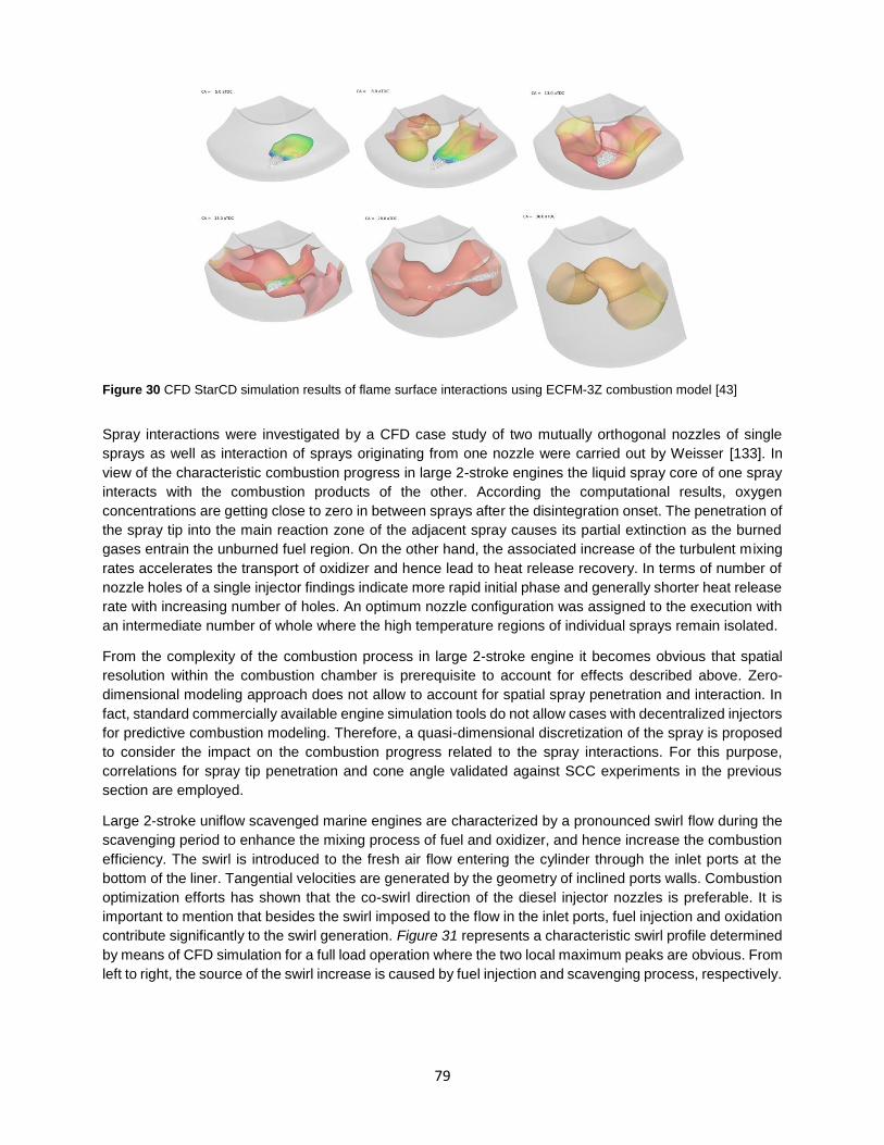
79
Figure 30 CFD StarCD simulation results of flame surface interactions using ECFM-3Z combustion model [43]
Spray interactions were investigated by a CFD case study of two mutually orthogonal nozzles of single
sprays as well as interaction of sprays originating from one nozzle were carried out by Weisser [133]. In
view of the characteristic combustion progress in large 2-stroke engines the liquid spray core of one spray
interacts with the combustion products of the other. According the computational results, oxygen
concentrations are getting close to zero in between sprays after the disintegration onset. The penetration of
the spray tip into the main reaction zone of the adjacent spray causes its partial extinction as the burned
gases entrain the unburned fuel region. On the other hand, the associated increase of the turbulent mixing
rates accelerates the transport of oxidizer and hence lead to heat release recovery. In terms of number of
nozzle holes of a single injector findings indicate more rapid initial phase and generally shorter heat release
rate with increasing number of holes. An optimum nozzle configuration was assigned to the execution with
an intermediate number of whole where the high temperature regions of individual sprays remain isolated.
From the complexity of the combustion process in large 2-stroke engine it becomes obvious that spatial
resolution within the combustion chamber is prerequisite to account for effects described above. Zero-
dimensional modeling approach does not allow to account for spatial spray penetration and interaction. In
fact, standard commercially available engine simulation tools do not allow cases with decentralized injectors
for predictive combustion modeling. Therefore, a quasi-dimensional discretization of the spray is proposed
to consider the impact on the combustion progress related to the spray interactions. For this purpose,
correlations for spray tip penetration and cone angle validated against SCC experiments in the previous
section are employed.
Large 2-stroke uniflow scavenged marine engines are characterized by a pronounced swirl flow during the
scavenging period to enhance the mixing process of fuel and oxidizer, and hence increase the combustion
efficiency. The swirl is introduced to the fresh air flow entering the cylinder through the inlet ports at the
bottom of the liner. Tangential velocities are generated by the geometry of inclined ports walls. Combustion
optimization efforts has shown that the co-swirl direction of the diesel injector nozzles is preferable. It is
important to mention that besides the swirl imposed to the flow in the inlet ports, fuel injection and oxidation
contribute significantly to the swirl generation. Figure 31 represents a characteristic swirl profile determined
by means of CFD simulation for a full load operation where the two local maximum peaks are obvious. From
left to right, the source of the swirl increase is caused by fuel injection and scavenging process, respectively.

80
Figure 31 CFD calculated swirl number SN over the entire cycle at full load conditions [43]
The level of swirl motion is expressed in form of a swirl number SN (91) which depends on the angular
velocity and engine speed. The swirl number can be calculated from the initial flow velocity and the
inclination angle in the inlet ports. Subsequently, the tangential velocity can be determined as swirl velocity
at the corresponding radius utan= /r
𝑆𝑁 =
2𝑛 (90)
Based on the tangential velocity profile across the cylinder diameter the swirl in large 2-stroke engine can
be classified as forced vortex that can be approximated as solid body rotation. However, concerning the
majority of physical problems, such a rough simplification does not correspond to the real conditions. The
Rankine swirl profile presents a better approximation of the flow within the combustion chamber as
confirmed by the measurements of Nakagawa [89]. The overall angular momentum of the Rankine swirl
corresponds to the total angular momentum of the solid body rotation. It can be further simplified by a
polynomial form of a third grade according to (91) for the instantaneous tangential velocity utan over the
radius r where rtot correspond to the outer radius of the cylinder liner. For the present case, constants of the
polynomial terms are tuned according to the CFD simulation results represented by a solid line in Figure 37.
𝑢𝑡𝑎𝑛 = 𝑢𝑡𝑎𝑛,𝑚𝑎𝑥 [𝐶1 (
𝑟
𝑟𝑡𝑜𝑡
) + 𝐶2 (𝑟
𝑟𝑡𝑜𝑡
)2
+ 𝐶3 (𝑟
𝑟𝑡𝑜𝑡
)3
] (91)
In case of confined swirl, the tangential velocity increases proportionally with radius until it is damped in the
wall boundary layer and ultimately reaches zero at the wall. Two different calculated profiles of the tangential
swirl velocity utan over the cylinder radius at full load conditions of RT-flex60 engine are shown in Figure 32.
In addition, a result of detailed CFD calculation with zero flow condition on the wall boundary is included in
the plot for the reference. The impact on the spray penetration and interactions will be discussed further.

81
Figure 32 In-cylinder swirl profiles of tangential flow velocity plotted over cylinder radius
A state of the art diesel injector for a large 2-stroke engine has five nozzle holes differentiating in the nozzle
diameter and in both horizontal and vertical angles of each nozzle hole. Depending on the actual geometry,
injection timing and fuel pressure, the individual sprays penetrate into the combustion chamber and interact
with the swirl flow. To determine the influence on the spray in each time step, the position history of each
spray tip has to be tracked in time after the SOI. The resulting spray tip velocity determining its position in
the following time step is a result of a vector addition of the initial spray velocity and local tangential velocity
of the in-cylinder flow. The mass of a fuel package is defined by fuel mass flow through an individual nozzle
(92) and the amount of entrained air within a time step. The entrained air mass into the fuel package is
calculated according to (93) by employing the law of momentum conservation.
𝑚𝑓 = 𝐶𝐷
𝜋𝑑𝑛𝑜𝑧𝑧𝑙𝑒2
4√
2(𝑝𝑓 − 𝑝𝑐𝑦𝑙)
𝜌𝑓
(92)
𝑚𝑎𝑖𝑟 = 𝑚𝑓 (
𝑢𝑓,0
𝑢𝑓
− 1) (93)
In order to account for the different momentum of the fuel and the entrained air mass within a single package,
the initial tangential velocity determined from the swirl profile is corrected by the mass ratio resulting in the
final deflection velocity that changes the spray trajectory as defined in (94). The constant Cdefl determines
to what extent is the direction of the penetrating spray affected by the in-cylinder swirl in respect of the
entrained air mass.
𝑢𝑑𝑒𝑓𝑙 = 𝐶𝑑𝑒𝑓𝑙 (
𝑚𝑎
𝑚𝑎𝑖𝑟 + 𝑚𝑓
) 𝑢𝑡𝑎𝑛 (94)
In Figure 33 the geometrical interpretation of the spray tip velocity originating from a single injector nozzle
hole is introduced. Geometry of individual nozzle holes as well as the impact of the swirl motion and air
entrainment rate are accounted for in the mathematical model. Based on a simple trigonometric scheme
representing the engine and injector geometry together with boundary conditions for injected fuel and swirl,
the resulting spray velocity uspray is a product of a vector addition. This comprises of the initial spray tip
velocity from the preceding time step, deflection velocity determined from the in-cylinder spray profile at the
actual position of the spray tip and the impact of momentum conservation.
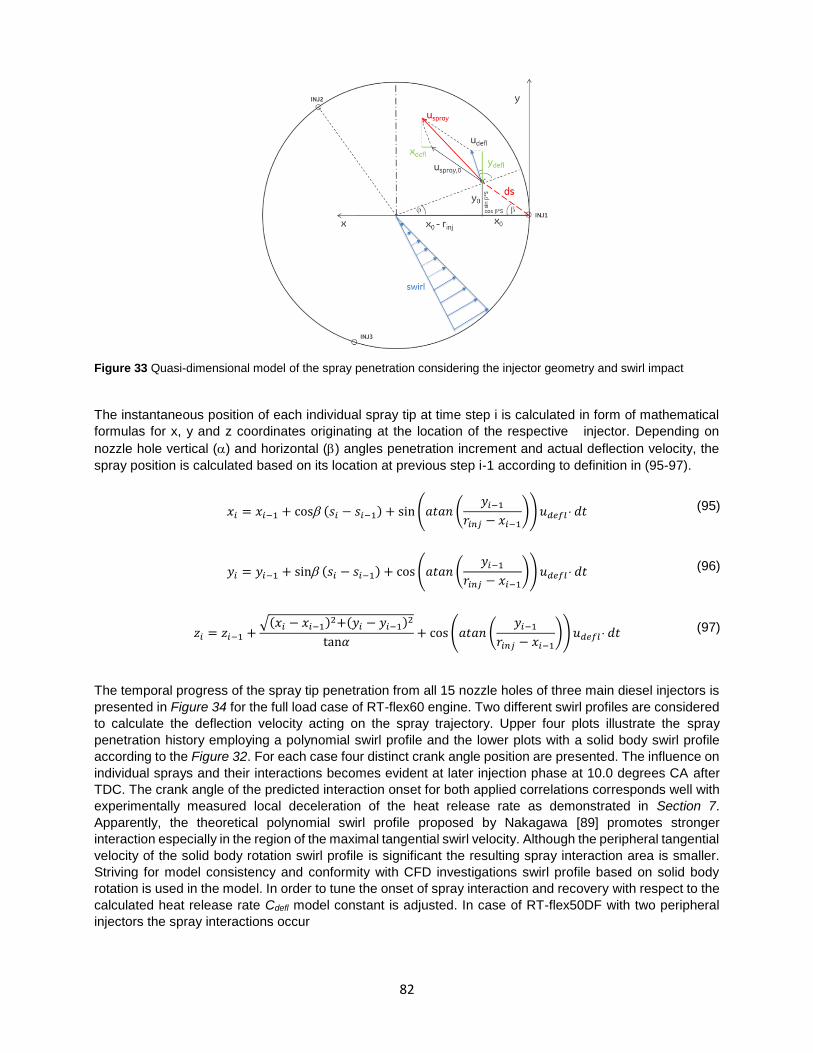
82
Figure 33 Quasi-dimensional model of the spray penetration considering the injector geometry and swirl impact
The instantaneous position of each individual spray tip at time step i is calculated in form of mathematical
formulas for x, y and z coordinates originating at the location of the respective injector. Depending on
nozzle hole vertical () and horizontal () angles penetration increment and actual deflection velocity, the
spray position is calculated based on its location at previous step i-1 according to definition in (95-97).
𝑥𝑖 = 𝑥𝑖−1 + cos (𝑠𝑖 − 𝑠𝑖−1) + sin (𝑎𝑡𝑎𝑛 (
𝑦𝑖−1
𝑟𝑖𝑛𝑗 − 𝑥𝑖−1
))𝑢𝑑𝑒𝑓𝑙 𝑑𝑡 (95)
𝑦𝑖 = 𝑦𝑖−1 + sin (𝑠𝑖 − 𝑠𝑖−1) + cos (𝑎𝑡𝑎𝑛 (
𝑦𝑖−1
𝑟𝑖𝑛𝑗 − 𝑥𝑖−1
))𝑢𝑑𝑒𝑓𝑙 𝑑𝑡 (96)
𝑧𝑖 = 𝑧𝑖−1 +
√(𝑥𝑖 − 𝑥𝑖−1)2+(𝑦𝑖 − 𝑦𝑖−1)
2
tan𝛼+ cos (𝑎𝑡𝑎𝑛 (
𝑦𝑖−1
𝑟𝑖𝑛𝑗 − 𝑥𝑖−1
))𝑢𝑑𝑒𝑓𝑙 𝑑𝑡 (97)
The temporal progress of the spray tip penetration from all 15 nozzle holes of three main diesel injectors is
presented in Figure 34 for the full load case of RT-flex60 engine. Two different swirl profiles are considered
to calculate the deflection velocity acting on the spray trajectory. Upper four plots illustrate the spray
penetration history employing a polynomial swirl profile and the lower plots with a solid body swirl profile
according to the Figure 32. For each case four distinct crank angle position are presented. The influence on
individual sprays and their interactions becomes evident at later injection phase at 10.0 degrees CA after
TDC. The crank angle of the predicted interaction onset for both applied correlations corresponds well with
experimentally measured local deceleration of the heat release rate as demonstrated in Section 7.
Apparently, the theoretical polynomial swirl profile proposed by Nakagawa [89] promotes stronger
interaction especially in the region of the maximal tangential swirl velocity. Although the peripheral tangential
velocity of the solid body rotation swirl profile is significant the resulting spray interaction area is smaller.
Striving for model consistency and conformity with CFD investigations swirl profile based on solid body
rotation is used in the model. In order to tune the onset of spray interaction and recovery with respect to the
calculated heat release rate Cdefl model constant is adjusted. In case of RT-flex50DF with two peripheral
injectors the spray interactions occur

83
Figure 34 Progress of spray penetration and interaction at full load operation for polynomial (upper plot) and solid body
rotation (lower plots) swirl profiles for RT-flex60 and RT-flex50DF engines.
Figure 35 illustrates schematically progress of spray penetration and dispersion in early combustion phase
around 10.0 degrees CA after TDC for three and two injector engine versions. Apparently, for the three
injectors version the interaction between spray and burned gases originating from upstream injector has
already started whereas in two injectors version majority of injected fuel can be burned freely. For modeling
purpose, the influence of spray interactions on the resulting burn rate is interpreted in form of
instantaneously available fuel already evaporated and mixed within the flammability limits.
Figure 35 Spray interactions for engines with three and two injectors without a swirl impact

84
To describe spray interactions and determine the effective spray surface area associated with the total flame
area determining the oxidation rate, instantaneous surface area is calculated for each spray. This is done
by combining the conical surface with the apex angle corresponding to the dispersion angle of an individual
spray and a hemisphere forming the spray tip as shown on the sketch in Figure 35. Such approach
corresponds better to the experimental observations in terms of actual spray shape than approximation the
spray by a simple cone. From trigonometry, the hemisphere radius rtip can be determined by trigonometric
relation (98) from the spray dispersion angle defined by the equation (89) and spray penetration s resulting
from (87) and (88). Note that this approach follows assumption that the spray remains of ideal conical shape
merely bended by the deflection velocity resulting from swirl motion resulting.
𝑟𝑡𝑖𝑝 =
tan 𝜃/2 𝑠
(1 + tan 𝜃/2) (98)
As illustrated on Figure 36, the total surface area of a single spray can be determined as a sum of areas of
a hemispherical front part corresponding to the spray tip attached to the cone representing the spray body.
Figure 36 Spray surface approximation by a geometrical area of hemispherical spray tip adjacent to a cone surface
representing the spray body with dispersion angle
Such a geometrical spray representation can be described by the equation (99). The first term on the right
side stands for the tip hemisphere volume and the second term represent the cone surface. In order to
obtain the total spray area, equation (99) is applied to all individual sprays and the resulting areas are
summed up.
𝐴𝑠𝑝𝑟𝑎𝑦 = 2 𝑟𝑡𝑖𝑝
2 + 𝑟𝑡𝑖𝑝√ 𝑟𝑡𝑖𝑝2 + (𝑠 − 𝑟𝑡𝑖𝑝)
2 (99)
Quasi-dimensional model calculates the interacted spray area based on penetration and dispersion history
of individual sprays according to (100). As the burned gases originating from the upstream injector reach
the fresh fuel, the interacted area is calculated as a difference of a free lateral spray cone surface with the
length x subtracted from the entire spray surface determined for the full penetration length s. The length x
is calculated based on mutual spray position of x and y coordinates according to Figure 39. Recovering of
the heat release rate depends on the difference of instantaneous velocities of interacted sprays at the
location of interaction uspray,i . The recovering of the heat release rate corresponds to the reduction of the
interacted spray area. This reduction is determined by the area defined by the interacted length multiplied
by the distance in propagation direction of the interacted spray. The point of interaction onset is denoted by
xi,interact.
𝐴𝑠𝑝𝑟𝑎𝑦,𝑖𝑛𝑡𝑒𝑟𝑎𝑐𝑡 = ∑𝐴𝑠𝑝𝑟𝑎𝑦,𝑖 − 𝑟𝑥,𝑖 (√ 𝑟𝑥,𝑖
2 − (𝑥𝑖 − 𝑟𝑥,𝑖)2) + (𝑥𝑖 − 𝑥𝑖,𝑖𝑛𝑡𝑒𝑟𝑎𝑐𝑡)∆𝑢𝑠𝑝𝑟𝑎𝑦,𝑖𝑑𝑡
𝑛
𝑖=1
(100)

85
The ratio of spray area interacting with burned gases from the upstream injector to the total area determines
the available evaporated fuel that can be burned in actual time step. Following this concept, the unburned
fuel available for the diffusion combustion is given by equation (101). Index j identifies specific nozzle hole
and n denotes the total number of injector holes.
𝑚𝑓,𝑢,𝑑𝑖𝑓𝑓 = 𝑚𝑓,𝑢,𝑒𝑣𝑎𝑝
∑ (𝐴𝑠𝑝𝑟𝑎𝑦,𝒋 − 𝐴𝑠𝑝𝑟𝑎𝑦,𝑖𝑛𝑡𝑒𝑟𝑎𝑐𝑡,𝒋)𝒏𝒋=𝟏
∑ 𝐴𝑠𝑝𝑟𝑎𝑦,𝒋𝒏𝒋=𝟏
(101)
In general, the fuel total fuel mass can be divided into five imaginary pools as presented in Figure 37. The
distribution among those pools I, II and III is driven by corresponding models related to fuel injection, spray
formation and breakup, evaporation and mixing with oxidizer as described in previous sections. Spray
interactions discussed in the present section govern the allocation of the already evaporated and mixed fuel
to the pool IV representing the amount of available unburned fuel ready for oxidation. To quantify the
magnitude of interacted spray area, both total free and interacted flame areas are calculated based on
correlations for spray tip penetration and dispersion accounting for the impact of swirl as described by
equations (91-101).
Figure 37 Diesel spray combustion model structure describing fuel transformation path
The process of fuel injection, evaporation interaction and oxidation is plotted dimensionless mass scaled in
Figure 38. Due to the low engine speed fuel evaporation and mixing is nearly negligible and corresponds to
approximately half a crank angle. For the lower flammability limit of the diesel fuel equivalence ratio of 1.67
is assumed. The flame interaction ratio is defined by the fraction on the right side of equation (101). As soon
as the spray interaction is initiated the available fuel for combustion is limited. After termination of the
injection the remaining fuel is transported more rapidly into a region with available oxygen and is eventually
burned. The simulated late combustion phase and the associated combustion efficiency depends primarily
on turbulence model and its dissipation.
Figures 38 Simulated fuel mass fraction transition at full load engine operation

86
5.4 Ignition Delay and Premixed Combustion Models
Ignition of diesel fuel depends on multiple factors such as fuel properties, injector geometry, nozzle tip
execution, injection pressure or engine operation determining the in-cylinder thermodynamic conditions.
Moreover, number of chemical reactions taking place in various temperature and time regimes are essential
in terms or resulting ignition delay. Commonly employed correlations for engine cycle simulations assume
an averaged ignition delay linked to a global reaction involving all intermediate steps and states of individual
processes. Such approximation can be justified for the present model since the ignition delay compared to
the combustion duration is negligible. Hence, a simplified empirical approach is implemented in form of
Livengood-Wu integral in which the immediate ignition time is determined as a function of in-cylinder
pressure and temperature history by equation (102) according to Stringer [117] Intentionally, dependencies
on additional parameters e.g. on equivalence ratio were omitted due to both lack of experimental data and
redundancy.
𝜏𝑖𝑔𝑛 = 𝐶𝑖𝑔𝑛 𝑝
−0.75𝑒(5473
𝑇) (102)
Experimental ignition delay was measured on SCC from the effective injection start until occurrence of OH
luminescence. Reported results [125,126] show strong dependency of the ignition delay on ambient gas
temperature whereas other parameters such as nozzle orifice diameter, fuel quality or excess air ratio have
rather a minor impact. Figure 39 shows averaged ignition delay based on SCC experiments with LFO fuel
at 90bar and 900K ambient pressure and temperature, respectively. Additionally, full scale engine
measurements are plotted for two engine types with different compression ratio. In this case the ignition
delay is determined as a time between the initial injection pressure rise and the positive value of heat release
rate calculated based on cylinder pressure analysis. Finally, correlated results employing the ignition integral
approach according to (102) are plotted in solid lined.
Figure 39 Ignition delay based on SCC experiments, engine measurements and calculated by integral approach
The adopted Arrhenius type correlation employed in the developed diesel combustion model predicts similar
time necessary for ignition as measured experimentally in SCC. However, an attempt to match the employed

87
correlation both with SCC result and full engine ignition delay is not feasible. The reasons are twofold. First,
due to substantial differences in ignition delay determination the SCC results based OH luminescence can
report SOC immediately whereas the measurable increase of indicated cylinder pressure due to combustion
start on a full-scale engine can be detected as the combustion already progresses. Moreover, generally
much lower accuracy of full scale engine measurements plays also an important role. For the RT-flex50DF
engine with reduced compression ratio resulting in lower in-cylinder temperature the mismatch becomes
substantial. Hence, the correlation can be adjusted by finetuning corresponding coefficients.
Typically, for today’s efficiency-optimized 2-stroke marine diesel applications the premixed combustion is
negligible. However, for DF engine applications with low compression ratio it becomes more pronounced
and needs to be considered in the modeling approach. In the present work, concept relying on the
characteristic premixed time scale ign is employed following the approach defined in [132]. The ignition
delay period is decisive in terms of fuel amount prepared to be directly oxidized immediately after
combustion start. The fuel burned within the premixed combustion model is defined as the fraction
evaporated during the ignition delay according to equation (103), where mf,u,prem denotes unburned fuel
evaporated during the ignition delay and available for premixed combustion.
𝑑𝑚𝑓,𝑏,𝑝𝑟𝑒𝑚
𝑑𝑡= 𝐶𝑝𝑟𝑒𝑚
1
𝜏𝑖𝑔𝑛
𝑚𝑓,𝑢𝑛,𝑝𝑟𝑒𝑚 (103)
5.5 Diesel Turbulence model
Diesel diffusion oxidation rate is primarily governed by a turbulent mixing process characterized by turbulent
intensity u’ and characteristic diffusion length scale ldiff. In order to calculated the turbulence intensity u’,
simplified zero-dimensional turbulence model is derived following the conceptual approach outlined in the
theory section based on work of various studies [6,21,36]. The employed turbulence model relies on the k-
model formulation. Even though this approach was intentionally tailored for planar shear layers, a good
performance was shown when simplifying for 0D problems in reciprocating engines [7,24] as well.
Summarizing the main assumption for the present applications, the turbulence kinetic energy is assumed
homogeneous, isotropic and is determined from the mean flow kinetic energy. Hence, production terms of
the turbulent kinetic energy can be assigned to major source terms and designated as kinetic energy of the
main flow field. In this way, a simplified description of a complex turbulent flow is feasible by a zero-
dimensional or quasi-dimensional method. Specifically, kinetic energy of the injection spray, density
variations and swirl motion are considered relevant production source terms in the present model according
to equation (104).
(𝑑𝑘
𝑑𝑡)𝑝𝑟𝑜𝑑
= (𝑑𝑘
𝑑𝑡)𝑑𝑒𝑛𝑠𝑖𝑡𝑦
+ (𝑑𝑘
𝑑𝑡)𝑠𝑤𝑖𝑟𝑙
+ (𝑑𝑘
𝑑𝑡)𝑖𝑛𝑗
(104)
The temporal change of the turbulent kinetic energy dk/dt is defined as a subtraction of the dissipation rate
form the turbulent kinetic energy production. In the theoretical Section 4.2, the basic principle of eddy
dissipation was introduced adopting the energy cascade concept. In the simplified model, no dissipation
into heat and influence on in-cylinder conditions is considered.
𝑑𝑘
𝑑𝑡= (
𝑑𝑘
𝑑𝑡)𝑝𝑟𝑜𝑑
− (105)
88
As consequence of the engine stroke, the production term based on compressibility effects influencing the
viscosity and Reynolds number is related to the density changes by equation (106) as proposed in [7].
(𝑑𝑘
𝑑𝑡)𝑑𝑒𝑛𝑠𝑖𝑡𝑦
=3
2𝑘
1
𝜌
𝑑𝜌
𝑑𝑡 (106)
For the formulation of the phenomenological combustion model the kinetic energy arising from the direct
fuel injection is of major importance since it directly impacts the turbulent mixing and fuel oxidation progress.
This is modelled by means of Rather a rather simple approach for determining the kinetic energy of the fuel
spray from the injection velocity defined by the Bernoulli equation and corresponding discharge coefficient.
Analogous to [118] the specific kinetic energy of fuel injection is obtained by relating the kinetic energy to
the total in-cylinder mass following equation (107).
(𝑑𝑘
𝑑𝑡)𝑖𝑛𝑗
= 𝐶𝑖𝑛𝑗1
2
𝑑𝑚𝑖𝑛𝑗
𝑑𝑡𝑢𝑖𝑛𝑗
21
𝑚𝑐𝑦𝑙
(107)
The effect of swirling flow on turbulence production is related to the radial distribution of angular momentum
in the cylinder and hence the production term is directly linked to the tangential velocity. Assuming
approximation of the mean flow by a solid body rotation, shear stresses are not considered and the utan is
proportional to the radius adopting the conservation of angular momentum. In the reality, the swirl profile in
the engine cylinder is a combination of solid body rotation and free vortex where the tangential flow velocity
is proportional to the reciprocating value of the cylinder radius. Since Reynolds stresses are negative the
swirl motions suppress the turbulence in a way that the kinetic energy is transferred back to the mean flow
with stabilizing effects. However, as the swirl is generated by the flow through inclined inlet ports close to
the BDC piston position, turbulent flow is generated. For the sake of simplicity and considering
implementation into a 1D cycle simulation tool where the cylinder volume is not spatially resolved an average
tangential velocity in the inlet port is employed. The tangential component is calculated by the decomposition
of the average flow velocity adopted directly from the 1D cycle simulation using basic trigonometry applied
on the inclined design of inclined inlet ports. The specific kinetic energy production by the swirl generated
at inlet ports is averaged over the total cylinder mass.
(𝑑𝑘
𝑑𝑡)𝑠𝑤𝑖𝑟𝑙
= 𝐶𝑠𝑤𝑖𝑟𝑙 1
2
𝑑𝑚𝐼𝑃
𝑑𝑡𝑢𝑡𝑎𝑛
21
𝑚𝑐𝑦𝑙
(108)
Interactions with surrounding fluid are not explicitly accounted for but are indirectly considered in the
dissipation rate coefficient. During the compression phase the swirl vortex is being squashed. Nevertheless,
since the swirl vorticity is proportional to the length scale and density, it remains constant since both length
scale and density change proportionally during compression as no squish is present in the large 2-stroke
marine engines. In general, the turbulent kinetic energy related to the swirl source term and generated
predominantly at inlet ports is damped and decays during the compression stroke as obvious from resulting
profiles discussed below. Nevertheless, the definition of the initial TKE level together with the density
production term prior to fuel injection onset is determinative for the subsequent combustion process.
Dissipation of the turbulent kinetic energy cannot be modeled in detail when employing a zero-dimensional
turbulence model. The utilized concept relies on the dissipation proportionality to the turbulence intensity

89
and the integral length scale defined in equation (29). Transforming the turbulence intensity to the turbulent
kinetic energy for a 0D isotropic, homogenous conditions yields relation (109).
𝑢′3
𝑙𝑖𝑛𝑡
= 𝐶𝑑𝑖𝑠𝑠1
𝑙𝑖𝑛𝑡
𝑘3/2 (109)
The integral length scale associated to the in-cylinder turbulence can determined from the instantaneous
cylinder volume as the diameter of the equivalent a spherical shape as defined by equation (110).
𝑙𝑖𝑛𝑡 = (
6 𝑉𝑐𝑦𝑙
𝜋)1/3
(110)
The model constants of individual turbulent kinetic energy source terms were tuned to match an averaged
TKE profiles calculated by means of CFD at various engine loads. For this purpose, the user combustion
model was implemented in a 1D cycle simulation tool and the TKE history was tracked during the scavenging
phase from inlet port opening (IPO) at 144.5 DATDC until termination of the combustion as presented in
Figure 40. Comparing the detailed CFD results with the adopted zero-dimensional turbulence model, the
results show desired agreement through the entire cycle. However, several differences can be discussed.
Apart from the early phase differences arising from boundary conditions, flow pattern and timestep
resolution, there is a slight overestimation in the turbulence production during the compression phase. On
the other hand, as regards TKE determination during the combustion phase, where the calculated burn rate
is governed by the turbulent mixing process, the reduced model shows good fidelity.
Figure 40 0D turbulence model results compared against CFD calculation at 25% engine load
Variation of engine load according the propeller curve results into differences in in-cylinder flow filed and
fuel injection rate. These changes affect directly source terms for the TKE production and modify its history
as shown in crank angle resolved plot in Figure 41. During the initial phase as inlet ports are opened the
turbulent kinetic energy is directly determined from the averaged velocity profiles predominantly by the swirl
source term (107). Obviously, pressure difference between scavenging pressure and in cylinder pressure
defining so called blow-back phase is governing the TKE generation. Within the compression stroke the
most of the generated TKE is dissipated whereas the increase towards the TDC is related to the density

90
production term. Later, diesel fuel injection participates substantially on the turbulence increase during the
combustion phase.
Figure 41 TKE calculated by the present model at various loads for RT-flex60 engine
Apart from the source terms considered for the zero-dimensional turbulence model definition, from the
turbulence related theory Section 4.2 it is obvious that the combustion process generates a non-negligible
portion of TKE increase as the fuel conversion progresses. Together with engine bore size specific
differences affecting the in-cylinder flow the turbulence combustion source term is considered in the overall
diffusion coefficient Cdiff.
5.6 Diffusion Combustion Model
After the evaporated fuel during the ignition delay oxidizes the major part of the injected fuel is converted in
the diffusion combustion mode. The diffusion oxidation rate of evaporated fuel that is allocated within the
region with defined oxygen availability is defined by the time scale approach. Adopting the time scale model
concept introduced by Weisser [132] the reaction rate is calculated based on turbulent time scale analogous
to eddy breakup models used within CFD codes. The mixing controlled oxidation is governed predominantly
by the turbulence whereas kinetics is not dominant. The diffusion burn rate is formulated based on the
turbulent time scale 𝜏𝑇 and the available evaporated unburned fuel 𝑚𝑓,𝑢𝑛,𝑑𝑖𝑓𝑓.
𝑑𝑚𝑓,𝑏,𝑑𝑖𝑓𝑓
𝑑𝑡= 𝐶𝑑𝑖𝑓𝑓
1
𝜏𝑇
𝑚𝑓,𝑢𝑛,𝑑𝑖𝑓 (111)
The time scale is often denoted as large eddy turnover and represent the scale of the of the flow. Hence,
the turbulent time scale is essentially determined by the structure of the turbulent flow field. For the simplified
0D model an approximation related to the turbulent viscosity u’lI and a characteristic diffusion length scale
ldiff is used and the turbulent mixing frequency that is determined according to equation (112).
1
𝜏𝑇
=𝑢′ 𝑙𝐼
𝑙𝑑𝑖𝑓𝑓2 (112)

91
The characteristic length scale of relevance here is assigned to the largest eddies in the flow that are
predominant in terms of momentum and energy transport. Typically, the diffusion length scale is derived
from the mixing length of fuel and oxidizer and is associated with a characteristic dimension of the system.
Here, the volume-to-surface ratio of the cylinder volume and the total fuel spray area is used. The total fuel
spray area is defined as the sum of all individual spray areas resulting from spray penetration and
interaction. After the injection of fuel is terminated, the spray area is set to a constant equal to its value at
EOI.
𝑙𝑑𝑖𝑓𝑓 =
𝑉𝑐𝑦𝑙
𝐴𝑓𝑙,𝑡𝑜𝑡
(113)

92
6. Dual Fuel Model Formulation
6.1 Modeling Approach
For proper combustion model definition phenomenological aspects of the DF lean burn concept in large
uniflow scavenged 2-stroke engines with direct low pressure gas admission and micro-pilot ignition
(SR~99%) need to be considered. The relevant theory for premixed turbulent flame propagation and lean
combustion was summarized in Section 4.4. Generally, dual fuel combustion is distinguished by substantial
level of complexity related to both diffusive and premixed combustion regimes. Interactions between the
gaseous main fuel, oxidizer and diesel pilot fuel take place imminently during admission of gaseous fuel,
injection and oxidation of pilot fuel and finally within the main premixed combustion phase. In order to gain
a better understanding of individual phenomena, numerous multidimensional CFD studies were performed
including parameter variations relevant to gas admission and mixing process. Furthermore, CFD simulations
analyzing the impact of fuel mixture homogeneity, pilot fuel fraction and EGR on ignition delay and
combustion were performed. Within the process of model formulation, both results of adopted CFD
investigations and applied tabulated kinetics were employed.
During elaboration of the present work, the lean burn concept for large 2-stroke engine was in the early
development phase and hence immature. Therefore, extensive experimental research has been
accomplished including parameter variations and hardware selection to optimize engine performance and
make the concept ready for industrialization [89,94]. Besides variation of the relevant hardware such as
GAV nozzle geometry or turbocharging strategy optical combustion endoscopy was performed on a selected
cylinder of the full-scale RT-flex50DF research engine. The outcome of this work was valuable for
understanding the ignition and early combustion phase and to derive suitable submodels.
Typically, the maximum power output of state of the art lean burn 4-stroke engine is limited by the end gas
knock onset. However, experiments on large 2-stroke DF engines have shown that the maximum power
output is constrained rather by early combustion start. As a consequence of the early SOC cylinder firing
pressure reaches the design limit leading to the engine power output restriction. Therefore, developing a
methodology for engine knock prediction that would not rely on a commonly used empirical integral
approach was not prioritized in this study. Engine experiments have shown that the pre-ignition
phenomenon defined as a spontaneous flame kernel ignition prior to flame front arrival becomes more
severe with increasing engine load. Under regular engine operation clear jet from pre-chamber is observed
that ignites the unburned main chamber mixture. If exceeding the pre-ignition threshold, the ignition occurs
in multiple flame kernels simultaneously prior to ignition controlled by the pilot fuel injection. Such ignition
behavior was investigated for high BMEP gas engines by Yasueda et al. [140]. Figure 42 illustrates both
ignition modes based on combustion visualization results. According to these investigations the ignition of
the flammable mixture depends not only on engine load, gas quality or intake temperature but also on
stratification of the unburned gas air mixture. These findings were taken into consideration when developing
the turbulent premixed combustion model [20]. Based on findings described above the developed
phenomenological dual fuel combustion model need to consider both pilot fuel controlled and self-ignition
triggered ignition. Furthermore, interaction between pilot and main fuel, cylinder purity and stratification of
the gaseous fuel are together with the in-cylinder turbulence essential in terms of premixed turbulent dual
fuel combustion.

93
Figure 42 Combustion endoscopy at medium RT-flex60 engine load for two distinct cases. Left for regular pilot triggered
ignition, right pre-igniting controlled ignition with multiple flame kernels [100]
In this regard, Figure 43 illustrates the schematic structure of the dual fuel combustion model developed for
the 2-stroke lean burn gas engine. The blue arrays characterize the immediate computational sequence
and the red stand for feed back links. First of all, the thermodynamic state together with instantaneus
equivalence ratio and cylinder flow field pose major factor having impact on the combustion process. This
is triggered through shaping the level of laminar and turbulent flame velocities. It is also worth noting that
the second feed back path is associated with the pilot combustion which then define the global combustion
onset as a matter of preference. In general, the model features number of submodels according to the
diagram labeling specifically related to gas admission, pilot fuel injection, ignition delay for both pilot and
main fuels, correlations for laminar and turbulent flame velocities and finally the overall burn rate.
Figure 43 Schematics of the dual fuel combustion model structure
Whereas for the ignition delay of the pilot fuel simplified Livengood-Wu integral approach is suitable due to
high rest gas content and continuously hot conditions in the prechamber, tabulated values originating from
the detailed kinetics [120] are used to determine the ignition delay of the gaseous fuel. This is necessary to

94
account for varying in-cylinder composition as discussed later in Section 6.3. By separating the two distinct
ignition modes, a large degree of freedom in the model application is ensured. In this way combustion modes
triggered both by the pilot injection and merely by auto-ignition or the gaseous fuel can be considered. The
admission of gaseous fuel introduced during the scavenging period drives together with the swirling air
motion the turbulence production before combustion start. Moreover, gas admission valve (GAV) design
together with GAV timing and selected gas pressure impact the mixture homogeneity and thus influence the
resulting burn rate. In terms of the pilot fuel burn rate the approach is analogous to the concept incorporated
for the pure diesel diffusive combustion described in Section 5.5. Elevated temperature allows neglecting
the premixed part of liquid fuel burning without any effect on results. The premixed combustion of the main
gaseous fuel accounts for a highly complex process, hence an adequate reduction is prerequisite. Assuming
a homogenous fuel oxidizer mixture, even distribution of temperature and pressure within the cylinder as
well as uniform turbulence level the laminar and turbulent flame speeds can be approximated. The laminar
flame velocity is calculated using a correlation derived from predictions based on detailed chemistry
[119,120] and compared with past experimental investigations [38,94]. Moreover, the correlation was
extended using kinetic mechanism based data beyond the reported validity region. In this respect, the
approach may be exploited for engine relevant conditions. Following the work of various authors [7,24] the
in-cylinder zero-dimensional turbulence model is formulated based on mean flow history. Such methodology
presents a substantial reduction of the actual turbulence production and dissipation processes. Therefore,
the obtained mean kinetic energy is compared against averaged TKE calculated by CFD for multiple cases.
Subsequently, turbulent flame speed relationship suggested in [87] is employed utilizing the turbulence
intensity and the turbulent Reynolds number to the laminar flame speed in order to obtain final flame front
propagation. Eventually, the complete model is integrated into a GT-Suite 1D simulation tool by means of a
user routine. During the engine cycle simulation instantaneous parameter values related to in-cylinder
conditions, pilot injection pressure profile and admission of the main gaseous fuel are sent to the user code
which in turn determines the ignition delay and calculates the burn rate based on actual in-cylinder
conditions.
6.2 Pilot Fuel Combustion
A suitable formulation of the pilot combustion model is integral part of the DF combustion simulation
approach and is introduced first by the nature of the combustion progress. Considering a low-pressure lean
burn concept, the flammable mixture is ignited by pilot fuel towards the end of the compression stroke. Due
to the insufficient reactivity and additional stratification of the main fuel charge the absence of an
independent ignition source would prevent the fuel-oxidizer mixture from stable and repeatable ignition
event. That could lead to instabilities or cause complete flame front extinction especially at part load
conditions. Therefore, implementing of reliable combustion control methodology is prerequisite to ensure
both stable engine operation without knock or misfire and optimization of engine performance. Furthermore,
aiming for low engine-out emissions and diesel fuel demand the amount of the liquid pilot fuel is desired to
be minimized. In case of large marine DF engines, the mass related ratio of the pilot fuel compared to the
main shrinks down to a value close to 1% at full load without having a negative impact on the combustion
stability. On the other hand, the requirement for stable operation at low load contradicts the micro-pilot
strategy with direct injection into the main combustion space mainly due to the reduced compression end
temperature and spray dilution that aggravates ignitability. To overcome these challenges, a concept of
pilot combustion chamber (PCC) with an integrated injector inside of the chamber was selected. The PCC
is not actively scavenged, so that high temperature level caused by significant rest gas content is being
maintained over the entire engine cycle. Consequently, the ignition delay is not directly linked to the main
chamber conditions and remains negligible. High temperature level within the PCC accelerates oxidation

95
process of the pilot fuel and leads to a rapid pressure rise that generates an intense torch propagating
throughout the unburned mixture in the main combustion chamber in co-swirl direction. In conclusions,
outstanding combustion stability together with low unburned hydrocarbons emission over the entire
operating range including engine idling is ensured. Pilot fuel is supplied by a high pressure common rail
system that lessens variations in the injected mass amount among individual cylinders and allows short
energizing time for optimum interaction with the main fuel charge. It is worth noting that the balance between
rail pressure and energizing time for given pilot fuel amount is determinative to ensure rapid pilot
combustion for high momentum jet penetrating into the main chamber. Integration of the injector into the
PCC and as an assembly in the cylinder head is shown in Figure 44.
Figure 44 PCC assembly with pilot fuel injector integrated into engine cylinder head [91]
Being aware of the combustion system layout details, boundaries for the simulation model can be identified
and defined. Essentially, the energy release pattern resulting from the pilot fuel is approximated numerically
utilizing a similar concept applied for the pure diesel combustion as defined in Section 5. Yet, specific
processes correlative of the pilot fuel combustion in the PCC such as pilot jet penetration into the main
chamber causing turbulence effects followed by the entrainment of unburned fuel and oxidizer into the flame
zone need to be addressed. To capture the typical peak of the pilot burning in the total heat release rate,
thermodynamics of both pre-chamber and the main combustion chamber are considered. The provided
outcome of detailed CFD investigations is employed to provide further insight into the phenomena of pilot
combustion and develop individual sub-models accordingly.
The gas composition and temperature level in the PCC prior to the start of injection are directly coupled
with the rest gas content resulting from rather poor scavenging of the pre-chamber volume as demonstrated
in Figure 45. As shown, the initial conditions are characterized by an extensive rest gas content as well as
elevated temperature compared to the main combustion chamber state. This fact has a significant impact
on the combustion process taking place in the PCC. Ultimately, the thermodynamic state in the PCC is
being determined by interactions with the main chamber resulting from the instantaneous pressure
difference driving the gas exchange through the PCC outlet bore and in fact determining the propagation
of the pilot flame torch.

96
Figure 45 Multidimensional CFD analysis of the rest gas content and temperature distribution in the PCC at the end of
scavenging (left) and at the TDC (right) [108]
As already noted, the high temperature in the prechamber throughout the entire cycle leads to insignificant
ignition delay at all operating conditions. Therefore, ignition delay for the pilot can be approximated
empirically by using an Livengood-Wu type correlation without introducing any major discrepancy to the
reality. The combustion rate is calculated by adopting the time scale approach according to [132] following
the equation (114). The characteristic length scale of pilot combustion lpilot is defined as cube root of the
PCC volume and the turbulent intensity is calculated according to the approach defined for the zero-
dimensional turbulence for diesel combustion in Section 5.5.
𝑑𝑚𝑓,𝑏, 𝑝𝑖𝑙𝑜𝑡
𝑑𝑡= 𝐶
𝑢′
𝑙𝑝𝑖𝑙𝑜𝑡
𝑚𝑓,𝑢,𝑝𝑖𝑙𝑜𝑡 (114)
The mean kinetic energy equation according to (27) corresponding to the turbulent energy of the largest
scales is adopted to calculate turbulent intensity within the pilot combustion chamber. Reducing the
approach introduced in Section 5.5 while considering merely the turbulence source term arising from the
injected spray the original equation yields (115) for the pilot combustion case.
𝑑𝑘
𝑑𝑡=
1
2
𝑑𝑚𝑓,𝑝𝑖𝑙𝑜𝑡
𝑑𝑡𝑢𝑓,𝑝𝑖𝑙𝑜𝑡
21
𝑚𝑃𝐶𝐶
− 𝐶𝑑𝑖𝑠𝑠 ∙1
𝑙𝐼𝑘
32 (115)
The model constant for the dissipation was set to Cdiss = 0.2 by matching the predicted PCC pressure with
the measured pressure profile. Figure 46 illustrates integrated burn rate at full load conditions together with
injection rate profile and TKE progress both scale to the corresponding peak values. The model was
calibrated against measured pressure profiles in the PCC without partial validation of the submodels, e.g.
for TKE. Based on the fuel injection rate and the simulated burn rate conclusion can be made that the pilot
fuel oxidizes rapidly and the majority of the injected fuel is burned already within the injection phase.

97
Figure 46 progress of pilot fuel burn rate and corresponding non-dimensional profiles of injection rate and TKE
In the phenomenological DF modeling concept, the injection of pilot fuel does not only define the actual
combustion start of the main premixed gaseous fuel but also influence its initial progress. In this respect,
Figure 47 illustrates an example of an optical investigation and a corresponding multidimensional
calculation related to the pilot jet penetration during the initial combustion phase. Experimental results
generated in early phase of the 2-stroke DF engine development provide insights into ignition and flame
propagation which in turn allows to setup CFD simulation properly. The outcome of the CFD simulation
related to the PCC conditions and pilot jet propagation was utilized to develop and verify the present
modeling approach.
Figure 47 Experimental [100] and 3D CFD computational results of pilot jet penetration at early combustion phase [108]
The reduced model for the pilot torch penetration into the main chamber is based on calculation of the
prechamber pressure pPCC
calculation that is governed by the temperature rise within the PCC which is
given by the ratio of on average temperature linked to initial condition in the prechamber prior to injection
start and its adiabatic increase due to heat release of the pilot fuel. The initial pressure pPCC,0
is equal to
the in-cylinder pressure and the temperature TPCC,0 was adopted from CFD investigations presented in
Figure 48.
𝑝𝑃𝐶𝐶 = 𝑝𝑃𝐶𝐶,0 (𝑇𝑃𝐶𝐶
𝑇𝑃𝐶𝐶,0
)
−1
(116)

98
The pressure difference between the PCC volume and the main chamber determines the velocity of the
pilot flame torch at the PCC outlet. The actual value of the jet velocity at the PCC outlet is calculated
analogous to the gas flow through GAV defined by equation (124) based on the effective area of the PPC
oulet diameter. Subsequently, penetration length into the main chamber is calculated by conservation of
momentum where the air entrainment rate coefficient is tuned according to available CFD results following
the approach introduces in Section 4.2 taking into to account the swirl motion. Finally, the resulting pilot jet
volume is obtained from the penetration length and the pilot jet diameter as calculated in CFD in a form of
a truncated cone. Assuming an even distribution of the unburned gaseous fuel, the amount of gas directly
influenced by the pilot combustion is proportional to the jet volume generated by the penetrating diesel
flame. Therefore, the temperature input for the laminar flame velocity correlation is linked to the pilot jet
temperature until the volume directly influenced is consumed. Then, the unburned zone temperature is
taken into account again. Comparisons of calculated pressure in the pre-chamber against measurement
and of the pilot jet penetration against CFD results are presented on Figures 48 and 49, respectively.
Figure 48 Prechamber pressure history measured and calculated at 50% engine load
Figure 49 Pilot jet penetration calculation compared against CFD data for 50% engine load

99
6.3 Ignition Delay, Cylinder Discretization
Since the composition of natural gas may vary widely, determining the auto-ignition behavior changes
significantly under engine relevant conditions. Presence of higher hydrocarbons impacts reactivity which
may result in increased knock sensitivity or lower flammability, just to mention a few effects. Methane
number (MN) is determined by the volume of methane blended with other hydrocarbons and characterizes
the knock tendency that provides also valuable information related to the ignition delay. In addition to the
gas composition, the ignition delay of premixed gaseous fuel differs significantly depending on initial
conditions such as temperature, pressure or gas composition. There are additional effects having impact
on the actual ignition delay during engine operation such as mixture stratification, presence of hot spots or
impact of the lubrication oil.
Compared to the negligible and well-defined ignition delay of the pilot fuel in the PCC the auto-ignition of
the gaseous fuel cannot be simply determined based on the idea of a lumped bulk equation linked to the
averaged in-cylinder conditions. Moreover, there are no experimental auto-ignition data relevant for low
temperatures and gas compositions applicable on a lean burn concept of 2-stroke DF marine engines fueled
with low pressure NG. The operation at low speed and reduced compression ratio leads to prolonged
residential time of the admitted gas at low in-cylinder temperature level. Variable hydraulic exhaust valve
drive allows to adjust the effective CR and control the compression temperature. Furthermore, by variation
of exhaust valve opening and closing stratification level and cylinder purity are affected. These measures
influence the auto-ignition and the gas combustion substantially. Hence, the theoretical unburned zone
temperature at TDC in dependency of engine load and ambient conditions needs to be identified for
optimum engine performance as well as for the ignition delay prediction of the premixed charge. Another
potential source of gas ignition is related to the direct lubrication of the cylinder liner walls. Interactions
between oil droplets and unburned gases may form multiple flame kernels that trigger uncontrolled
combustion. Experimental investigations on full scale DF test engine have only partially confirmed a direct
link between lubrication oil and auto-ignition at low loads. Therefore, the pre-flame reactions are governed
primarily by thermodynamic conditions and the impact of lubrication can be neglected. As mentioned above,
natural gas composition variations have direct influence on the ignition delay depending on the content of
higher hydrocarbons. Nevertheless, considering gas composition influence for ignition and combustion
modeling would increase the model complexity substantially. Moreover, due to missing relevant
experimental data and relatively low knock sensitivity of the 2-stroke DF engine the effect of gas
composition (MN) is neglected.
Employing an ignition delay mechanism linked to the mean thermodynamic conditions of the unburned zone
for calculations of various engine types has shown a significant discrepancy between simulation and
experimental results. Hence, it is obvious that the ignition delay determination approach based on the
average temperature is not applicable for capturing the real engine operation. This infers conclusion that
the primarily temperature driven ignition delay is not directly linked to the mean in-cylinder conditions but
strongly depends on spatial differences within the combustion space resulting from gas admission process,
scavenging efficiency, wall heat transfer and other factors. Local gas concentrations play an important role
during the ignition delay phase especially when rich mixture directly interacts with the high temperature
zone originating from hot rest gases located mainly below exhaust valve. This leads to a considerable
reduction of ignition delay characterized by advanced occurrence of combustion start and introduce a
discrepancy into the ignition prediction.
To capture spatial variations within the cylinder, a discretization methodology is proposed that accounts for
the local variation of burned fraction, temperature and gas concentrations. Schematics of the vertical
cylinder volume discretization methodology is illustrated in Figure 50.

100
Figure 50 Schematics of cylinder volume discretization employed for the quasi-dimensional ignition model
The total cylinder volume is equally divided into a user specified number of sub-volumes, i.e. zones. For
each zone the burned and unburned mass fractions are calculated according to instantaneous mass flows
at inlet ports and exhaust valve determined directly during a 1D cycle simulation from the engine model.
Governing equations for mass and energy conservation are formulated according to Macek [78] by
equations (117) and (118), respectively.
𝑑𝑚𝑖
𝑑𝑡= ∑
𝑑𝑉𝑖
𝑑𝑡
𝑛
𝑖=0
(𝜌𝑖−1𝑤𝑖−1,𝑖 − 𝜌𝑖+1𝑤𝑖,𝑖+1) + �̇�𝑖𝑛 − �̇�𝑒𝑥ℎ + �̇�𝑔 (117)
𝑑(𝑚𝑖ℎ𝑖)
𝑑𝑡= ∑
𝑑𝑉𝑖
𝑑𝑡
𝑛
𝑖=0
(ℎ𝑖−1𝜌𝑖−1𝑤𝑖−1,𝑖 − ℎ𝑖+1𝜌𝑖+1𝑤𝑖,𝑖+1) + 𝑚𝑖(ℎ𝑖−1𝑤𝑖−1,𝑖 − ℎ𝑖+1𝑤𝑖,𝑖+1)
+ 𝛼𝑄𝐴𝑖(𝑇𝑤𝑎𝑙𝑙 − 𝑇𝑖) + 𝑉𝑖
𝑑𝑝𝑖
𝑑𝑡
(118)
Mass fluxes are related to intake, exhaust and gas flows and become valid for relevant zones only.
Instantaneous transfer of burned gas and fresh air is computed between adjacent zones and defines the
burned mass fraction at the end of every time step. This is then determinative for the amount of transferred
burned and fresh gas within the following time step. Perfect mixing is assumed so that the zonal temperature
is defined by the burned mass fraction and the temperatures of both unburned and burned gases. Additional

101
increase of zonal temperature is due to the heat transfer from the wall which considers an empirical liner
temperature distribution approximation.
The assumption of a uniform pressure for all volumes has been made. It has to be also stated that the
influence of mass change due to chemical reaction and evaporation is not relevant since the cylinder
discretization is terminated upon combustion onset. In addition, the gaseous fuel concentration within an
individual volume is a result of the gas admission profile and the instantaneous cylinder volume which
defines the location of individual subvolumes with respect to the gas admission valve (GAV) position. Heat
transfer between individual zones is not considered for the present model, merely the heat flux from/into
cylinder walls is modeled for each subvolume proportionally to the overall in-cylinder wall heat transfer. Both
intake and exhaust mass flow data as well as gas flow per cylinder over engine crank angle obtained from
1D GT-Suite engine cycle simulation are plotted in Figure 51 for the full load operation conditions of RT-
flex50DF engine.
Figure 51 Temporal resolution of intake/exhaust and gas mass flow rates
To capture the gas exchange process with mixing of fresh scavenging air and gas with burned gas from the
preceding combustion it is sufficient to initiate the cylinder discretization subroutine at the inlet port opening
(IPO). Prior to IPO it is assumed that the cylinder volume contains only burned gas. Flow boundary
conditions for entering fresh air and burned gas are determined from the cycle simulation at each time step
for the first and last sub-volumes, respectively. During the gas admission period, an additional flow is
imposed at the location of the gas admission valve (GAV). The position of gas inlet flow remains constant
in relation to the TDC position, hence the different subvolumes are filled with gaseous fuel depending on
their actual position. Subsequently, the unburned gaseous fuel is mixed with fresh air and its concentration
within a subvolume is computed at each time step. In the present model, the gas flow through a single GAV
is defined by the equation (123) for compressible flow where pcyl is the in-cylinder pressure, is the ratio of
specific heats of the gaseous fuel, pg gas admission pressure and dGAV denotes the GAV nozzle diameter.
The gas density is calculated based on actual gas pressure and temperature.
Figure 52 illustrates zonal burned mas fractions and temperatures for vertical cylinder volume discretization
into 25 sub-volumes for full load operation of RT-flex50DF engine. These variables are tracked for over the
entire scavenging period starting at 145 CA degree before TDC as inlet ports opens and the cylinder volume
completely filled with combustion products. Based on the imposed boundaries according to Figure 51 zones
imminently adjacent to the inlet ports are facing the initial wave in the intake air flow that is reflected in zonal
burned mass fraction and temperature results. Unlike a standard cylinder object implemented in GT-Suite
library the quasi-dimensional model accounts for the engine stoke. Therefore, the wave induced by the
intake flow cannot be projected in volumes located further away from imposed flow boundaries. During the

102
compression phase volume of individual zone is defined as a fraction of the instantaneous cylinder volume
based on the total number of zones. As the fresh gas enters the cylinder and mixes with combustion
products the purity of individual sub-volumes increases. After inlet port closing the scavenging progress
decelerates for a while due to another pressure wave. This effect is visible especially for the upper zones
close to the exhaust valve. Similarly, concentration zonal temperature and equivalence ratio are determined.
The zonal burned mass fraction plotted on the left in Figure 52 is compared with cylinder averaged mass
burned fraction calculated using CFD. The model predictions are generally in agreement with the
multidimensional simulation. However, the resulting cylinder purity is somewhat overpredicted by the model
Figure 52 Zonal mass burned fraction (left) and temperature (right) employing the proposed cylinder discretization. Mass burned fractions is compared with cylinder averaged mass burned fraction simulated in CFD (dotted line)
Subsequently, the local conditions are compared against the tabulated ignition delay data graphically
represented in Figure 53 for various in-cylinder pressure and temperature levels as well as equivalence
ratios. Based on conditions in individual zonas the combustion starts when the calculated ignition delay
gets to zero. In case the ignition of the pilot liquid fuel precedes the self-ignition of the main gaseous fuel
the calculation based on the tabulated data is terminated. Model results and ignition delay prediction
accuracy are discussed in the results Section 7.
Figure 53 Tabulated ignition delay for initial pressure variation at phi=1 (left) and equivalence ratio variation at
p=80bar (right) for methane

103
6.4 Laminar flame speed
Premixed turbulent combustion is defined by the laminar flame front propagation. Under real engine
operating conditions the laminar flame front becames turbulent immedately after combustion start. However,
for modeling purpose it can be assumed that the flame behaves as laminar and the effect of turbulence is
superposed. Hence, prior to definition of the turbulent flame volocity governing the premixed combustion
modeling laminar flame velocity has to be determined.
Number of various correlations for laminar flame velocity based on past experimental investigation were
discussed in theory section [38,76,94,122]. However, only limited validity directly in terms of engine
operating conditions can be stated. The validity of particular correlation depends strongly on the success
rate in eliminating flame intrinsic instabilities linked to the effects of turbulent flow field. Moreover, depending
on applied measurement technique, data acquisition and post-processing methodology introduce additional
uncertainties. Besides these facts, the fundamental impracticability of experimental laminar flame velocity
determination under engine relevant conditions due to elevated pressure and very lean mixtures needs to
be considered as well. The theoretical background and causes were discussed previously within the Section
4.4.1. To provide a viable correlation for the present application a generic scheme should be considered
that covers targeted conditions. Such criterion requires an approach linked to a detailed mechanism rather
than employment of an experimentally determined relation. At the time of completion of the present work
there were no basic investigations of premixed flame propagation specifically suited for large 2-stroke dual
fuel engine application. Therefore, the selected computational approach adopts an existing correlation for
laminar flame propagation and was further validated against both detailed kinetics and experimental data
from literature. In this way, the physical based link between the global engine operating parameters and the
resulting flame front characteristic is ensured.
The approach adopting a polynomial function developed for lean conditions by Witt and Griebel [134] was
used as a basis for deriving a correlation determining the laminar flame front velocity propagation in this
study. After assessing several detailed mechanisms, the authors have chosen the GRI-Mech 3.0
mechanism [114] due to a comparably better performance especially for overstoichoimetric conditions at
elevated pressure. Although it was developed for gas turbine typical conditions, it has been also used for
automotive application with acceptable accuracy. Nevertheless, the validity of the correlation is constrained
to equivalence ratios 0.5-1.0, initial temperatures 473-823K at maximum pressure of 30bar which lies far
below an end compression pressure reference at combustion onset. Since these conditions are not fully in
agreement with characteristic in-cylinder thermodynamics of a DF lean burn engine, an additional validation
is imperative. It is also to be noted that the GRI-Mech 3.0 kinetic mechanism that was optimized and
validated primarily for ignition delay shock tube measurements at high temperatures above 1300K. More
recently, the mechanism was also evaluated for laminar flame velocity of methane-air mixtures
predominantly at ambient conditions [123]. Therefore, the overall mechanism validity within the targeted
area is constrained accordingly. Therefore, an adjusted reaction mechanism containing 79 species and 365
reactions was implemented for ignition delay and laminar flame velocity calculation [119,120]. The tabulated
mechanism includes dependencies on initial temperature, pressure, equivalence ratio, diesel fraction and
EGR. The latter is not relevant for the present study.
The laminar flame speed correlation is defined by equations (119), (120) and (121) originally suggested for
initial pressure from 7-30bar. As stated above, the equations have been adjusted to ensure accurate
response under relevant engine operation conditions. In particular, the pressure dependency of the constant
C2 in the equation (121) was tuned in order to fit the detailed kinetics computation results [120].
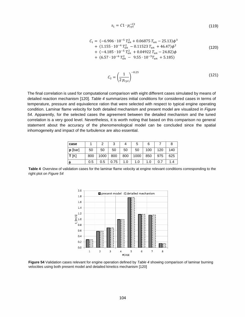
104
𝑠𝐿 = 𝐶1 ∙ 𝑝𝑐𝑦𝑙−𝐶2 (119)
𝐶1 = (−6.906 ∙ 10−5 𝑇𝑢𝑛2 + 0.06875 𝑇𝑢𝑛 − 25.13)𝜙3
+ (1.155 ∙ 10−4 𝑇𝑢𝑛2 − 0.11523 𝑇𝑢𝑛 + 46.47)𝜙2
+ (−4.185 ∙ 10−5 𝑇𝑢𝑛2 + 0.04922 𝑇𝑢𝑛 − 24.82)𝜙
+ (6.57 ∙ 10−6 𝑇𝑢𝑛2 − 9.55 ∙ 10−3𝑇𝑢𝑛 + 5.185)
(120)
𝐶2 = (
1
2 𝑝𝑐𝑦𝑙
)
−0.25
(121)
The final correlation is used for computational comparison with eight different cases simulated by means of
detailed reaction mechanism [120]. Table 4 summarizes initial conditions for considered cases in terms of
temperature, pressure and equivalence ration that were selected with respect to typical engine operating
condition. Laminar flame velocity for both detailed mechanism and present model are visualized in Figure
54. Apparently, for the selected cases the agreement between the detailed mechanism and the tuned
correlation is a very good level. Nevertheless, it is worth noting that based on this comparison no general
statement about the accuracy of the phenomenological model can be concluded since the spatial
inhomogeneity and impact of the turbulence are also essential.
case 1 2 3 4 5 6 7 8
p [bar] 50 50 50 50 50 100 120 140
T [K] 800 1000 800 800 1000 850 975 625
0.5 0.5 0.75 1.0 1.0 1.0 0.7 1.4
Table 4 Overview of validation cases for the laminar flame velocity at engine relevant conditions corresponding to the
right plot on Figure 54
Figure 54 Validation cases relevant for engine operation defined by Table 4 showing comparison of laminar burning
velocities using both present model and detailed kinetics mechanism [120]
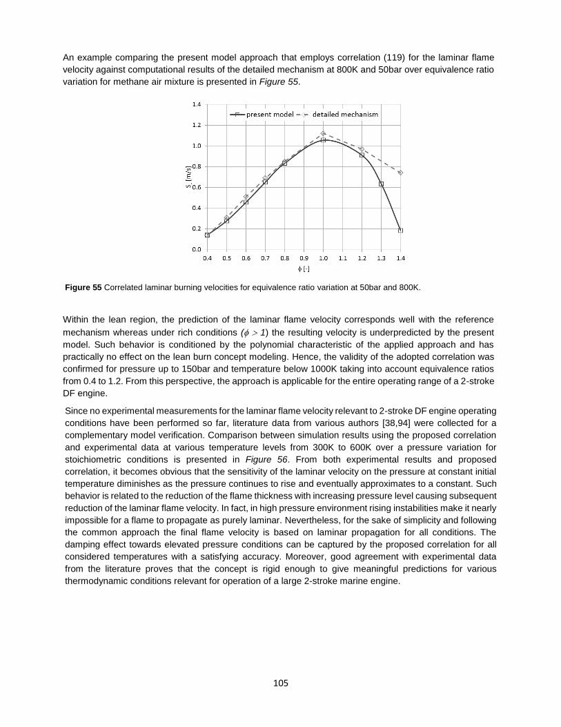
105
An example comparing the present model approach that employs correlation (119) for the laminar flame
velocity against computational results of the detailed mechanism at 800K and 50bar over equivalence ratio
variation for methane air mixture is presented in Figure 55.
Figure 55 Correlated laminar burning velocities for equivalence ratio variation at 50bar and 800K.
Within the lean region, the prediction of the laminar flame velocity corresponds well with the reference
mechanism whereas under rich conditions ( 1) the resulting velocity is underpredicted by the present
model. Such behavior is conditioned by the polynomial characteristic of the applied approach and has
practically no effect on the lean burn concept modeling. Hence, the validity of the adopted correlation was
confirmed for pressure up to 150bar and temperature below 1000K taking into account equivalence ratios
from 0.4 to 1.2. From this perspective, the approach is applicable for the entire operating range of a 2-stroke
DF engine.
Since no experimental measurements for the laminar flame velocity relevant to 2-stroke DF engine operating
conditions have been performed so far, literature data from various authors [38,94] were collected for a
complementary model verification. Comparison between simulation results using the proposed correlation
and experimental data at various temperature levels from 300K to 600K over a pressure variation for
stoichiometric conditions is presented in Figure 56. From both experimental results and proposed
correlation, it becomes obvious that the sensitivity of the laminar velocity on the pressure at constant initial
temperature diminishes as the pressure continues to rise and eventually approximates to a constant. Such
behavior is related to the reduction of the flame thickness with increasing pressure level causing subsequent
reduction of the laminar flame velocity. In fact, in high pressure environment rising instabilities make it nearly
impossible for a flame to propagate as purely laminar. Nevertheless, for the sake of simplicity and following
the common approach the final flame velocity is based on laminar propagation for all conditions. The
damping effect towards elevated pressure conditions can be captured by the proposed correlation for all
considered temperatures with a satisfying accuracy. Moreover, good agreement with experimental data
from the literature proves that the concept is rigid enough to give meaningful predictions for various
thermodynamic conditions relevant for operation of a large 2-stroke marine engine.
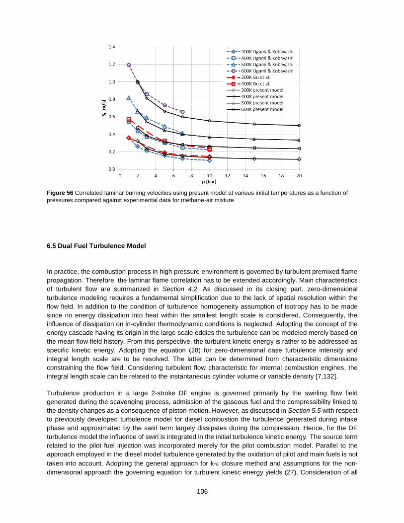
106
Figure 56 Correlated laminar burning velocities using present model at various initial temperatures as a function of
pressures compared against experimental data for methane-air mixture
6.5 Dual Fuel Turbulence Model
In practice, the combustion process in high pressure environment is governed by turbulent premixed flame
propagation. Therefore, the laminar flame correlation has to be extended accordingly. Main characteristics
of turbulent flow are summarized in Section 4.2. As discussed in its closing part, zero-dimensional
turbulence modeling requires a fundamental simplification due to the lack of spatial resolution within the
flow field. In addition to the condition of turbulence homogeneity assumption of isotropy has to be made
since no energy dissipation into heat within the smallest length scale is considered. Consequently, the
influence of dissipation on in-cylinder thermodynamic conditions is neglected. Adopting the concept of the
energy cascade having its origin in the large scale eddies the turbulence can be modeled merely based on
the mean flow field history. From this perspective, the turbulent kinetic energy is rather to be addressed as
specific kinetic energy. Adopting the equation (28) for zero-dimensional case turbulence intensity and
integral length scale are to be resolved. The latter can be determined from characteristic dimensions
constraining the flow field. Considering turbulent flow characteristic for internal combustion engines, the
integral length scale can be related to the instantaneous cylinder volume or variable density [7,132].
Turbulence production in a large 2-stroke DF engine is governed primarily by the swirling flow field
generated during the scavenging process, admission of the gaseous fuel and the compressibility linked to
the density changes as a consequence of piston motion. However, as discussed in Section 5.5 with respect
to previously developed turbulence model for diesel combustion the turbulence generated during intake
phase and approximated by the swirl term largely dissipates during the compression. Hence, for the DF
turbulence model the influence of swirl is integrated in the initial turbulence kinetic energy. The source term
related to the pilot fuel injection was incorporated merely for the pilot combustion model. Parallel to the
approach employed in the diesel model turbulence generated by the oxidation of pilot and main fuels is not
taken into account. Adopting the general approach for k- closure method and assumptions for the non-
dimensional approach the governing equation for turbulent kinetic energy yields (27). Consideration of all
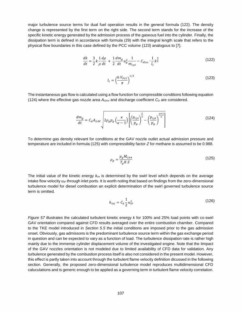
107
major turbulence source terms for dual fuel operation results in the general formula (122). The density
change is represented by the first term on the right side. The second term stands for the increase of the
specific kinetic energy generated by the admission process of the gaseous fuel into the cylinder. Finally, the
dissipation term is defined in accordance with formula (29) with the integral length scale that refers to the
physical flow boundaries in this case defined by the PCC volume (123) analogous to [7].
𝑑𝑘
𝑑𝑡=
3
2𝑘
1
𝜌
𝑑𝜌
𝑑𝑡 +
1
2
𝑑𝑚𝑔
𝑑𝑡𝑢𝑔
21
𝑚𝑐𝑦𝑙
− 𝐶𝑑𝑖𝑠𝑠 ∙1
𝑙𝐼𝑘
32 (122)
𝑙𝐼 = (
6 𝑉𝑃𝐶𝐶
𝜋)1/3
(123)
The instantaneous gas flow is calculated using a flow function for compressible conditions following equation
(124) where the effective gas nozzle area AGAV and discharge coefficient CD are considered.
𝑑𝑚𝑔
𝑑𝑡= 𝐶𝑑𝐴𝐺𝐴𝑉√2𝜌𝑔𝑝𝑔 (
− 1) [(
𝑝𝑐𝑦𝑙
𝑝𝑔
)
2
− (𝑝𝑐𝑦𝑙
𝑝𝑔
)
+1
] (124)
To determine gas density relevant for conditions at the GAV nozzle outlet actual admission pressure and
temperature are included in formula (125) with compressibility factor Z for methane is assumed to be 0.988.
𝜌𝑔 =
𝑝𝑔𝑀𝐶𝐻4
𝑇𝑔𝑅 𝑍 (125)
The initial value of the kinetic energy kini is determined by the swirl level which depends on the average
intake flow velocity uIP through inlet ports. It is worth noting that based on findings from the zero-dimensional
turbulence model for diesel combustion an explicit determination of the swirl governed turbulence source
term is omitted.
𝑘𝑖𝑛𝑖 = 𝐶𝑘
1
2𝑢𝐼𝑃
2 (126)
Figure 57 illustrates the calculated turbulent kinetic energy k for 100% and 25% load points with co-swirl
GAV orientation compared against CFD results averaged over the entire combustion chamber. Compared
to the TKE model introduced in Section 5.5 the initial conditions are imposed prior to the gas admission
onset. Obviously, gas admissons is the predominant turbulence source term within the gas exchange period
in question and can be expected to vary as a function of load. The turbulence dissipation rate is rather high
mainly due to the immense cylinder displacement volume of the investigated engine. Note that the Iimpact
of the GAV nozzles orientation is not modeled due to limited availability of CFD data for validation. Any
turbulence generated by the combustion process itself is also not considered in the present model. However,
this effect is partly taken into account through the turbulent flame velocity definition dicussed in the following
section. Generally, the proposed zero-dimensional turbulence model reproduces multidimensional CFD
caluculations and is generic enough to be applied as a governing term in turbulent flame velocity correlation.
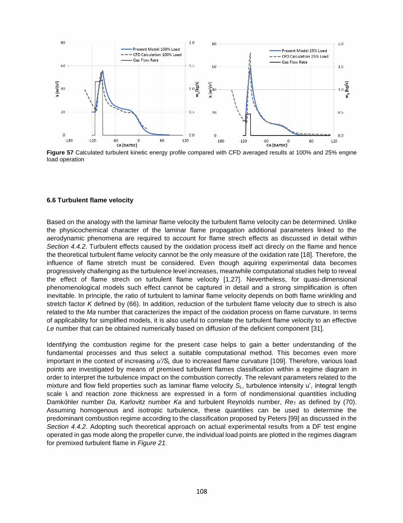
108
Figure 57 Calculated turbulent kinetic energy profile compared with CFD averaged results at 100% and 25% engine load operation
6.6 Turbulent flame velocity
Based on the analogy with the laminar flame velocity the turbulent flame velocity can be determined. Unlike
the physicochemical character of the laminar flame propagation additional parameters linked to the
aerodynamic phenomena are required to account for flame strech effects as discussed in detail within
Section 4.4.2. Turbulent effects caused by the oxidation process itself act direcly on the flame and hence
the theoretical turbulent flame velocity cannot be the only measure of the oxidation rate [18]. Therefore, the
influence of flame stretch must be considered. Even though aquiring experimental data becomes
progressively challenging as the turbulence level increases, meanwhile computational studies help to reveal
the effect of flame strech on turbulent flame velocity [1,27]. Nevertheless, for quasi-dimensional
phenomenological models such effect cannot be captured in detail and a strong simplification is often
inevitable. In principle, the ratio of turbulent to laminar flame velocity depends on both flame wrinkling and
stretch factor K defined by (66). In addition, reduction of the turbulent flame velocity due to strech is also
related to the Ma number that caracterizes the impact of the oxidation process on flame curvature. In terms
of applicability for simplified models, it is also useful to correlate the turbulent flame velocity to an effective
Le number that can be obtained numerically based on diffusion of the deficient component [31].
Identifying the combustion regime for the present case helps to gain a better understanding of the
fundamental processes and thus select a suitable computational method. This becomes even more
important in the context of increasing u’/SL due to increased flame curvature [109]. Therefore, various load
points are investigated by means of premixed turbulent flames classification within a regime diagram in
order to interpret the turbulence impact on the combustion correctly. The relevant parameters related to the
mixture and flow field properties such as laminar flame velocity SL, turbulence intensity u’, integral length
scale lt and reaction zone thickness are expressed in a form of nondimensional quantities including
Damköhler number Da, Karlovitz number Ka and turbulent Reynolds number, ReT as defined by (70).
Assuming homogenous and isotropic turbulence, these quantities can be used to determine the
predominant combustion regime according to the classification proposed by Peters [99] as discussed in the
Section 4.4.2. Adopting such theoretical approach on actual experimental results from a DF test engine
operated in gas mode along the propeller curve, the individual load points are plotted in the regimes diagram
for premixed turbulent flame in Figure 21.

109
BMEP [bar] 6.9 10.9 13.6 17.3
0.36 0.40 0.41 0.46
pcyl [bar] 41 56 68 75
u' [m s-1] 3.83 4.31 4.656 5.041
SL [m s-1] 0.45 0.50 0.53 0.65
u'/SL 8.42 8.64 8.71 7.80
lI [m] 0.0144 0.0144 0.0147 0.0150
[m] 4.81E-05 4.39E-05 4.10E-05 3.39E-05
lI/ 2.99E+02 3.28E+02 3.59E+02 4.43E+02
Da 36 38 41 57
Ka 1.41 1.40 1.36 1.03
ReT 2.52E+03 2.83E+03 3.13E+03 3.45E+03
K 0.222 0.220 0.213 0.162
k [m] 4.05E-05 3.71E-05 3.52E-05 3.33E-05
Table 5 Overview of turbulent flame relevant parameters related to selected engine operation points
Table 5 summarizes main turbulence related parameters for engine load variation for RT-flex50DF. The
conditions are considered prior to the combustion start at a temperature level of about 800K. Investigated
cases are located along the line separating corrugated flamelets and distributed / thin flame reaction regimes
as Karlovitz number is close to unity or slightly higher. For the selected points the regime diagram shows
that the turbulent intensity is larger than the laminar flame speed. Therefore, the turbulent motion can
generates fresh and burnt gas pockets within the wrinkled flame front. At such conditions the turbulence
influences the premixed zone but the reaction zone retains its wrinkled but to a certain extent still laminar
character. In addition, for Da values larger than one the flame time scale (d/SL) is smaller than the
characteristic eddy time (lI/u’) and so the turbulence does not have a strong impact on the flame structure.
However, the Kolmogorov scales appear to be smaller than the flame thickness, hence the flame is not
laminar having a wrinkled character. These findings were confirmed also experimentally [62] showing that
even though the modifications of contour spacing or curvature are not singnificant at elevated turbulence
level the turbulent effects still predominate and are determinative for the burning rate increase. The analysis
also reveals non negligible stretch rate which, especially at lower load points and at high overall air excess
ratio, indicates the tendency to extinction but is still distant from the limit for correponding equivalence ratio
[16].
In Section 4.4.2 several correlations for the turbulent premixed flame speed were presented and discussed
in terms of application and validity range. Figure 58 shows an overview of various concepts for turbulent
flame velocity determination at conditions relevant to real operation conditions summarized in Table 5. For
this comparison, the turbulent Reynolds number was considered ReT= 3x10³ and pressure ratio p/p0 = 1.5
if applicable are considered. Based on this comparison, individual correlations differ substantially from each
other. Possible causes of these differences are related to applied measurements methodologies, varying
boundary conditions and computational assumptions as well as due to the complexity of turbulent flame as
such. Comparing the correlated results with turbulent burning rates plotted in Figure 23 selected correlation
[39,61] are not in argreement with general trends. In previous simulation studies related to turbulent
premixed flames, several concept were adopted. Whereas in [37] the resulting flame propagation is resolved
as a simple scalar of laminar flame velocity and turbulence intensity in [95] the concept of Gülder [39] is
utilized. The latter approach is relativ insensitiv to the ratio of characteristic velocities u’/SL at constant ReT.
Unfortunately, without a direct link to experimental data the selection of a suitable correlation for turbulent
flame velocity cannot be validated. However, plotting the actual measurements points in the regime diagram
in Figure 21 reveals that for present application the turbulent flame is classified in thin reaction zone with

110
more intense turbulence leading to flame wrinkling and accelaration of the burn rate. Due to consistency of
reaction zone the turbulent flame front can be described by laminar flamelets [97]. This on the one side
justify the selected modeling approch with laminar flame velocity. On the other side, based on the thin
reaction turbulent regime the correlation for turbulent flame velocity should consider the the effect of
enhanced oxidation rate resultig from the wrinkled flame structure.
Figure 58 ST/SL values against u’/SL representing different correlations presented in Section 4.4.2
The present model adopts the correlation according to Dinkelacker [27] in order to account for effects
associated to flame stretch. The corresponding turbulent flame velocity is determined according to equation
(77). As discussed above, the Lewis number Le characterizes the turbulent premixed flame structure and
thus impacts the final burning rate substantially. In order to determine its effective value, an analytical
correlation following the approach in [31] is used taking into account both Lewis numbers of the unburned
fuel and oxidizer and their concentrations following equation (127).
Leeff=1+
(𝐿𝑒𝑂2 − 1) + (𝐿𝑒𝐶𝐻4 − 1)(1 + 𝛽(𝛷 − 1))
2 + 𝛽(𝛷 − 1) (127)
where is equal to for fuel-rich mixtures and 1/ for fuel-lean conditions. Such definition allows
considering excess air ratio changes related to the load variation or conditions. In this way instability effects
occurring especially at very lean mixtures can be considered for the phenomenological combustion model.
6.7 Dual Fuel Combustion
The transition from the flame front propagation into the actual burn rate is done by assuming a spherical
penetration of the turbulent flame front originating from the pilot flame jet as described in the following
section. The swirl motion induced by the inlet ports and further enhanced by the co-swirl gas admission is
beneficial both for improving the mixing of reactants and to secure highest possible combustion efficiency
by steering the flame propagation in the favorable way. This effect is further enhanced by pointing the PCC

111
outlet in the flow swirl direction. The combustion chamber layout featuring two opposite pilot pre-chambers
which are located on the circumference is schematically illustrated in Figure 59. For the sake of simplicity
essential for fast running model application, homogenous distribution of both temperature and gaseous fuel
is assumed. Moreover, no impact of rest gas, swirl and natural gas composition is considered for the burn
rate calculation. The progress of the dual fuel combustion process characterized by pilot fuel injection and
ignition within the PCC, burning jet penetration into the main combustion space, subsequent ignition of the
premixed gaseous fuel and the resulting flame front propagation through the main chamber.
Figure 59 Schematic representation of the combustion chamber and the flame front propagation
As already stated, the ignition delay is determined for both liquid and gaseous fuel as simulation progresses.
In design mode the combustion start is triggered solely by the pilot injection timing. Hence, burn rate
calculation depends on the flame front propagation defined by premixed flame turbulent velocity, flame front
area, unburned zone conditions as well as combustion progress variable according to equation (128).
𝑑𝑚𝑏,𝑔
𝑑𝑡=
𝜌𝑢
1 +1𝜙
∙ 𝐴𝐹𝑅𝑠𝑡
𝑆𝑇 ∙ 𝐴𝑓𝑙 (128)
The theoretical flame area correlation relies on the simplified spherical flame front propagation induced by
the pilot fuel combustion with respect to the combustion chamber geometrical boundaries according to the
equation (129). The flame radius rfl is determined from based on the time elapsed from the combustion start
and the instantaneus turbulent flame velocity ST. Following the work of Dinkelacker [27] characteristics of
the turbulent premixed flame structure in terms of flame wrinkling resulting from the flame strech are
accounted for in the adopted correlation for turbulent flame speed (77) in form of effective Lewis number.
Pilot jet inclination and impact swirl direction are neglected.
𝐴𝑓𝑙 = 4 ∙ 𝜋 ∙ 𝑟𝑓𝑙
2 1
12∙ (1 − 𝑥𝑏)
(129)
The flame thickness is infinitesimal relatively to the combustion chamber dimensions which allows to neglect
the difference between the inner and outer flame radius. In addition, the fact that the flame propagation
during the initial inflammation phase corresponds exclusively to the laminar velocity is not taken into
account. Therefore, the mean flame radius can be derived as a product of actual turbulent burning velocity
defined in the equation (77) and the elapsed time. It is self explaining, that such a simplified approach
neglects flame quenching in the vicinity of cold walls or the flame front disintegration due to stretch,
inhomogeneity and turbulent flow field. However, it is shown in the results that the impact of doing so on the
model accuracy is not significant. In case the autoignition process becomes predominant which is mainly

112
relevant for full load operation, combustion onset is defined by the ignition of the gaseous fuel only.
Nevertheless, the calculation of the global burn rate remains the same.

113
7. Results
7.1 Diesel Model Results
7.1.1 Experimental Setup and Data Acquisition
Diesel combustion is validated against experimental data from engines varying in bore size, compression
ratio or number of injectors. Table 6 summarizes key engine parameters of three large 2-stroke diesel
marine engines at CMCR operation. All are equipped with exhaust turbocharger with fixed geometry turbine
and feature electronically controlled common-rail injection system as well as variable exhaust valve
actuation. Whereas the RT-flex50DF has two peripheral injectors and reduced CR optimized for dual fuel
operation RT-flex60 and W-X72 have three injectors per cylinder to ensure proper atomization and
distribution of the injected fuel amount and high CR for optimum engine efficiency. These engine types were
selected intentionally to cover various specification and sizes of large marine low speed engines.
Engine type RT-flex50DF (RTX-5)
RT-flex60 (RTX-4)
W-X72
Number of cylinders 6 4 6
Bore [mm] 500 600 720
Stroke [mm] 2050 2250 2500
Compression ratio 12.0 18.45 18.8
Engine speed [rpm] 124.0 114.2 84.8
BMEP [bar] 17.3 21.0 20.5
Injectors per cylinder 2 3 3
Injector nozzle 212.DF.V03 213.LLb12h 220.A2.Std
Table 6 Specifications summary at CMCR for reference engine types
Reference measurements for model validation were done on full scale test or customer engines. Cylinder
pressure was indicated on all cylinders and used for determining the experimental heat release rate (HHR).
In general, measurements used were taken over 100 consecutive cycles averaged over time and engine
cylinder number. It is worth noting that the cylinder pressure analysis is performed with variable polytropic
coefficient but neglecting wall heat losses as described in the Section 7.2.1 in detail. Hence, the model
predictions in terms of combustion progress are compared in a form of apparent heat release rate with the
corresponding experimental HRR data.
7.1.2 Engine Load Variation
The developed modeling approach is integrated in the 1D engine cycle simulation tool GT-Suite by means
of a user subroutine programed in Fortran code. Input parameters such as in-cylinder conditions, injection
profiles or model constant are defined directly in the user code or are transferred through the user code
reference object and user code harness variables. The code structure follows the model layout as presented
in Figure 29. Even though majority of the input variables are passed to the code by default call functions to
simplify the model integrity selected signals are sensed directly via wiring harness and need to be added to
the model by the user. The 1D model layout in the GT-Suite environment is analogous to the DF model
shown in appendix Figure A1. Standard two-zonal combustion model is adopted and the thermodynamics
are calculated with the predefined real-gas model based on Redlich-Kwong equation of state. For diesel
operation user heat transfer model is employed, details are given in the Appendix A3.

114
Fuel injection pressure represents the key parameter determining the resulting burn rate. This occurs due
to impact on elementary phenomena such as spray atomization, penetration, dispersion, evaporation and
mixing. Increasing the injection pressure ultimately raises the turbulence intensity, which in turn accelerates
both mixing and oxidation processes. From the engine performance perspective, the fuel injection pressure
allows to find an optimum for combustion efficiency and emissions formation. Therefore, the model response
to injection pressure variation is essential regarding the model application for optimization studies. Before
the effect of rail pressure variation on the combustion can be analyzed, the injection rate needs to be
determined. For the fast running engine models, the use of an injection rate map has proven beneficial
especially due to low computational demand and high flexibility. The AMESim simulation code was used to
run detailed hydraulic simulation of the common-rail injector. The reliability of the numerical results was
tested through a comparison between numerical and experimental results when using marine diesel oil
(MDO) fuel. Subsequently, a broad map over variations of rail pressure and energizing time was generated
and used as an input for the ‘Multiple Pulse Injection Connection’ object convenient for DI diesel engines.
This setup allows not only to control the injection duration at target pressure for specific engine load but also
to implement different injection strategies such as sequential injection or pre-injection. Figure 60 presents
the injection rate map for the RT-flex60 engine ranging from 500 to 1400bar fuel rail pressure. If using the
model outside the injection rate map the profile are extrapolated accordingly. In case there are no injection
data available and the demand on high fidelity injection profile persists, detailed hydraulic injector model
can be coupled to the engine model within GT-Suite environment as demonstrated in Section 7.3.1. Due to
the very low engine speed the hydraulic delay determining the gap between the injection command and the
effective injection start at the nozzle exit can be neglected. However, pressure drop between the rail
pressure hold value and the effective injection pressure needs to be considered as discussed in [127]. For
the RT-flex60 engine with standard injector 100bar pressure drop is considered. For RT-flex50DF and W-
X72 with sacless fuel injector concept (FAST) 250bar difference between the rail and effective injection
pressure levels is applied.
Figure 60 Injected mass contour for the RT-flex60 engine based on ‘InjectionRateMap’ definition
To assess the performance of the developed combustion model, both crank angle resolved HRR and key
performance figures are evaluated. Key variables such as engine load, fuel rail pressure, nozzle execution,
injection patterns or engine type are varied. Model results are compared with experiments and discussed.
Figure 61 compares the simulated specific HRR and cylinder pressure history over RT-flex60 engine load
variation with the experimental measurements. Engine settings details and further load points are shown in
appendix Table A1. The model coefficients related to the zero-dimensional turbulence model and quasi-

115
dimensional spray interaction are tuned primarily for the full load operation point and are kept constant for
the remaining load points according to Table 7. In this way generic prediction capability of the modeling
approach can be assessed.
Figure 61 RT-flex60 simulated specific HRR and cylinder pressure history compared with measurements
Based on the comparison with experiment, at every load point the combustion onset, temporal progress,
point of interaction as well as the late combustion phase are well captured by the model. Especially the full
load point at 21.0 bar BMEP reproduces the experimental HRR profile in a plausible way. When reducing
the load, the initial phase of the heat release tends to be overpredicted. Consequently, also the point of
spray interactions occurs earlier than measured. This also causes that the late burning phase is slightly
accelerated. However, in the late combustion phase after the fuel injection is terminated the turbulence level
dissipates dramatically and the burn rate progress becomes disordered. In the present model the gradient

116
of the burn rate tail can be adjusted by both controlling the burn rate recovery after the spray interaction and
turbulence dissipation coefficient. Obviously, the model settings are determined based on comparison with
experimental heat release rate and predicted engine performance.
7.1.3 Fuel Rail-Pressure Variation
The fuel rail pressure that defines the effective injection pressure impacts directly the spray penetration,
dispersion, turbulence and other effects governing the fuel oxidation process. Comparison of predicted and
experimental heat release rates for rail pressure variation at 100% and 75% load is shown in Figure 62.
Model response on the rail pressure follows well the trend observed in measurements. While increasing the
fuel rail pressure the combustion becomes faster and the spray interactions are getting less pronounced.
These effects can be attributed to the higher turbulence promoting the mixing and faster oxidation,
respectively. The latter is related to the enhancement of atomization and evaporation so that the introduced
fuel oxidizes faster. Moreover, the combustion progress recovery occurs faster since the unburned fuel exit
the zone of burned gases more rapidly due to its higher momentum. Although the proposed model captures
well effects of rail pressure variation an overprediction can be stated in terms of initial combustion rate at
increased injection pressure. On the other hand, the late burning phase is delayed with respect to the
measurement especially at 75% engine load cases.
Figure 62 Model results for RT-flex60 rail pressure variation at 100% and 75% engine load

117
7.1.4 Injector Nozzle Execution Variation
Another key parameter affecting the spray characteristic is the injector geometry and more specifically the
nozzle execution. Experimental engine results with five different nozzle executions were selected to be
compared with model predictions at full load RT-flex60 engine operation. All injector nozzle executions have
identical holes angles but the diameter of individual holes was varied. Aiming for similar injection duration
time fuel rail pressure was elevated with reducing nozzle diameter as demonstrated in Figure 63.
Figure 63 Diesel model results for RT-flex60 nozzle execution variation at 100% engine load
Detailed comparison of simulated and measured specific heat release profiles is shown in Figure 64.
Generally, model predictions match the measurement results with good accuracy both in respect of
combustion start and HRR profile.
Figure 64 Model predicted and measured RT-flex60 HRR for injector nozzle execution variation at 100% load

118
Nevertheless, variations in the heat release restriction and relaxation due to spray interactions depending
on the nozzle executions are simulated qualitatively but no quantitatively when compared with experiments.
More specifically, HRR predictions for the largest and smallest nozzle executions deviate in spray interaction
onset defining the HRR deceleration as well as in the local HRR maximum due to combustion recovery. In
case of the largest nozzle (213.LLb12h) the calculated interaction of sprays is more pronounced and occurs
later than measured whereas for the smallest nozzle opposite behavior can be observed. Such model
behavior is linked to the determination of the interacted flame area by the quasi-dimensional spray
interaction model and partly also to the turbulence production and dissipation at elevated injection pressure.
7.1.5 Sequential Injection Impact
Various injection strategies such as pre-injection or injection rate shaping are common to optimize the
engine performance and emissions. For large 2-stroke marine engine with multiple injectors also sequential
injection presents a possibility for improving the efficiency while keeping the desired emission level. The
user routine based concept of the proposed diesel combustion model allows simple integration of multiple
injectors per cylinder and implementation of such injection patterns. Alternatively, the total desired injection
profile can be defined with using single injector object only. Such approach is also appropriate when
investigating the impact of injection rate shaping strategies. Typically, when adopting sequential injection
strategy individual injectors are actuated with delay in swirl direction to reduce the initial burn rate and hence
moderate the rapid increase of temperature. In this way nitric oxides can be reduced and enhancement of
the engine efficiency and emissions trade-off can be reached. Therefore, advancing the injection timing and
even adjusting the fuel rail pressure is necessary. Figure 65 shows the simulated HRR and the fuel injection
patterns with respect to injected mass flow rate for full load operation of the RT-flex60 test engine at constant
injection start and fuel rail pressure of 800bar.
Figure 65 Simulated specific HRR with sequential injection strategy at 100% engine load constant SOI and 800bar fuel
rail pressure
The sequential injection pattern is defined by crank angle delay for second and third injectors as denoted in
the HRR plot legend. Although the injection start is controlled individually the end of injection is synchronized
to minimize the late burning phase duration. Together with the baseline case without sequential injection
two other cases reflecting usual settings of the sequential injection are plotted in Figure 66. More
pronounced delay introduced to the injector in co-swirl direction results in deceleration of the initial
combustion phase as the available fuel is reduced. Due to the delayed injection timing the onset of the spray

119
interaction is slightly retarded. After recovery the remaining fuel is oxidized in a prolonged late combustion
phase. To compensate such delay, the fuel injection timing and pressure have to be adjusted for real engine
operation. The phenomenological model shows good level of prediction for sequential injection approach. If
desirable, it can be easily extended for simulating pre-injection or rate shaping strategies.
7.1.6 Engine Type and Bore Size
To ensure the generic validity the phenomenological diesel combustion model is employed in various engine
types defined in Table 6. Implementing the predictive user model in 1D GT-Suite environment requires only
a minor change of any existing 1D engine model by adding the dynamic link library file into the model folder
and linking corresponding parameter signals to wiring harness interface. Nevertheless, tuning of model
constant is necessary to optimize the model performance and address specific engine differences that
influence the combustion such as clearance volume, compression ratio or injector nozzle geometry.
Therefore, a sensitivity study of the main combustion model constants has been performed for engine load
variation of each engine type. Table 7 summarizes key model constants for both diffusion and premixed
oxidation rates, zero-dimensional turbulence definition and the spray interaction model. As stated in the
mode development Section 5.
Constant Equation RT-flex50DF
(RTX-5) RT-flex60 (RTX-4)
W-X72
Cdiff (111) 0.4 0.55 0.3
Cprem (103) 0.03 0.03 0.03
Cign (102) 0.15 0.1 0.1
Cinj (107) 0.2 0.2 0.1
Cswirl (108) 0.024 0.024 0.024
Cdiss (109) 2.0 1.6 2.0
Cdefl (94) 0.15 0.2 0.15
utan,max (91) 20.0 m.s-1 23.0 m.s-1 20.0 m.s-1
Table 7 Engine type specific model constants and key injection parameters
Figure 66 compares the specific heat release profiles for the three engines at full load operation both
predicted by the developed model and measured. In all three cases the simulated HRR correspond to
measurements in terms of start of combustion, spray interaction occurrence and combustion duration.
Figure 66 Comparison of specific heat release rate from different engines at full load operation

120
Despite the objective for generic combustion model there are few specifics related to engine type that need
to be discussed. Figure 67 illustrates predicted specific heat release rates for load variation for W-6X72
engine compared to experimental results. For this specific engine, no detailed fuel injection rate profiles
based on detailed hydraulic simulation were available. Instead, simple rectangular profiles were adopted
considering merely the necessary time for full injector needle lift. In consequence, the early injection phase
does not include any pronounced local peak. The simplified injection rate characteristic reflected in
deceleration of the initial HRR gradient. Furthermore, the model prediction overestimates the HRR global
maximum particularly at high and medium engine load cases. The cause for this behavior is related to the
delayed onset of spray interactions that decrease the instant HRR. Simulation at 25% and 10% engine load
match the experiment in terms of heat release progress and elimination of spray interaction impact but
shows somewhat prolonged late burning phase. Hence, the recommended adjustment of model constants
is related mainly to larger cylinder bore and longer piston stroke having impact on turbulence production
and dissipation as well as on in-cylinder flow field determining spray interactions. The presented comparison
with test data reveals potential of further model refinement primarily with respect to the engine type specific
phenomena governing the initial HRR slope, onset of HRR restriction and its recovery. These effects are
linked to the turbulence model predictivity and fidelity of capturing spray interactions.
Figure 67 Model predicted and measured HRR for W-X72 engine load variation
Considering model usage for another engine type RT-flex50DF several major differences need to be
considered with respect to the combustion model validation. First, the engine features only two peripheral
injectors instead of three. In addition, the compression ratio is reduced to meet the requirements for gas
operation. These differences lead to lower end compression temperature and the mutual position of both
injectors influences spray interactions. Based on the analysis presented in Section 5.4 ignition delay integral
approach tuned for the high compression ratio is not applicable for the DF engine version and the
corresponding constant Cign needs to be adjusted accordingly. Figure 68 compares predicted and
121
experimental heat release rates for a load sweep for a gas optimized RT-flex50DF engine. It is worth noting
that the data used for validation originate from an early development phase and hence does not present a
final optimized version. Nevertheless, a fair comparison can be done based on the available data. Clearly,
the ignition and the general progress of fuel oxidation is well captured by the model. However, the spray
interaction causing the local drop of the HRR shows differences in terms of timing and gradient. Further
refinement of the model with respect to the available fuel for instantaneous oxidation would be required for
better agreement. The late combustion phase is predicted with good accuracy except for the 10% load point
where the heat release is overpredicted by the model. Therefore, the late combustion phase is terminated
untimely since the entire fuel amount is already consumed.
Figure 68 Model predicted and measured HRR for RT-flex50DF engine load variation in diesel mode
7.1.7 Diesel Model Performance Assessment
Figure 69 summarizes the results of the complete set of variations considered in the present validation study
(33 selected experimental measurements listed in Table A1 in appendix) in the form of six plots of key
performance parameters. For every plot the x-axis shows experimental results and the y-axis model
predictions, with dashed lines denoting error bands of 1% (upper row) and 1 respectively 2 (rightmost
diagram) degrees crank angle (bottom row). The simulation is targeting the measured BMEP while the fuel
flow is determined by a PID controller. Upper left and right plots illustrate maximum firing pressure PMAX
and the determined diesel fuel flow both predicted mostly within the 1% error band. The remaining plots
present model performance in terms of ignition delay and combustion phasing. Start of combustion (SOC)
reflects the ignition delay calculation where the error does not exceed one crank angle unit. Note that data
points above the full line center axis refer to the RT-flex50DF engine, on which a longer ignition delay is
observed than determined by the model. The combustion phasing is characterized by the crank angle

122
position of 50% fuel mass fraction burned (MFB50). For the majority of the cases predicted MFB50 lies
within the ±1°CA accuracy interval. However, the model predictions of combustion phasing tend to be
slightly overestimated. This becomes even more pronounced when considering the combustion duration
determined as crank angle interval between the start of combustion and 90% of fuel mass burned. Generally,
the spread gets larger and most of the calculated points are located on the edge of the ± 2°CA accuracy
band. This indicates that during the late combustion phase the calculated heat release may proceed at a
lower rate than during the experiment. Nonetheless, one may conclude that the model accuracy is at a good
level and in spite of engine type related differences in model HRR prediction, general model performance
is meeting the requirements for fast running and generic engine cycle simulation.
Figure 69 Diesel model performance compared with measurement in respect of key performance parameters

123
7.2 Dual Fuel Model Results
7.2.1 Experimental Setup and Data Acquisition
The proposed model has been extensively validated against experimental data of full scale large 2-stroke
low speed DF engines. Data from two different DF engines types were utilized for comparing simulation and
test results. Table 8 provides an overview of key design specifications and major performance parameters
at CMCR operation for both engine types. The RT-flex50DF engine was used for the dual fuel concept
development to determine optimum performance parameter settings, turbocharger matching and define the
gas admission relevant component design. During the concept development phase, numerous engine
specifications and concepts were investigated and assessed. A broad database of experimental data has
allowed comprehensive model verification over a wide range of engine settings and operation conditions.
Engine type RT-flex50DF W-X72DF
Number of cylinders 6 6
Bore [mm] 500 720
Stroke [mm] 2050 2250
Compression ratio 12.0 12.0
Engine speed [rpm] 124.0 87.2
BMEP [bar] 17.3 17.3
GAV per cylinder 2 2
Injectors / PCC per cylinder 2 / 2 3 / 2
Table 8 Dual fuel engines specification overview at CMCR operating conditions
The Wärtsilä RT-flex50DF (RTX-5) test engine shown in the Figure 70. The engine is equipped with
electronically controlled common rail fuel injection and electro-hydraulic exhaust valve actuation and pilot
combustion chambers (PCC) accommodated in the cylinder head. Engine control system includes
functionalities such as speed controller, performance optimization, knock and misfire detection or various
safety algorithms including machinery protection. Full instrumentation and a data acquisition system were
installed on the test engine to capture all relevant parameters related to exhaust gas emissions, pressures,
temperatures, knock sensitivity as well as general engine and turbocharger performance readings
Figure 70 RT-flex50DF (RTX-5) engine test bed, free end and upper views

124
For cylinder pressure acquisition, high fidelity Kistler pressure sensors (type 6045B) were mounted in every
cylinder head and in selected pilot combustion chambers. Cylinder pressure history readings are acquired
in AVL LabView and further post-processed to perform heat release analysis. The final heat release profiles
are used for comparisons with the model predictions. The DF engine operation is driven by Wärtsilä UNIC
based control system
It is worth noting that the reference heat release is calculated using the cylinder pressure analysis based on
cylinder pressure history averaged over 300 cycles. In this way, uncertainties arising both from the
stochastic character of lean burn concept and the signal processing can be minimized. Furthermore, mean
cylinder pressure of the averaged ones from all individual cylinders is considered to eliminate variations
linked to charging, gas admission, pilot fuel injection or geometrical differences. Employing such
methodology within the entire operation range is eligible since covariance of cycle resolved IMEP and peak
firing pressure do not exceed 1.5% and 3%, respectively. In addition, the mean averaged cylinder pressure
is filtered with low pass filter to cut-off undesirable frequencies corresponding to any disturbance in the
signal acquisition chain or combustion chamber resonance frequency. In respect of premixed combustion
concept, the plausibility of the pilot fuel peak as well as characteristic knock frequency spectrum have to be
preserved. Potential source of error related to the pressure sensors accuracy and to the thermal shock error
should not exceed ±1% of IMEP according to specifications. Additional factors influencing the heat release
analysis accuracy substantially are the compression ratio together with the TDC position definition which is
determined during motoring operation. All relevant parameters having impact on the resulting HRR have
been proved carefully prior to each measurement campaign so the uncertainties can be minimized. The
HRR analysis has been performed directly in AVL Concerto tool using “Thermodynamics2” calculation that
stands for a fast heat release analysis with variable polytropic coefficient in relation to the in-cylinder
temperature. The calculation method considers only the energy effectively delivered to the gas while the
wall heat losses within the combustion space are being ignored. Hence, for comparison with the present
model apparent heat release need to be used assuming the wall heat losses are modeled appropriately.
The start of combustion (SOC) is defined by the crank angle as the HRR becomes positive. Equation (130)
defines the heat release per crank angle where C is a constant for unit conversion.
𝑄𝑖=
𝐶
𝑖 − 1𝑉𝑖+𝑛 [𝑝𝑖+𝑛 − 𝑝𝑖−𝑛 (
𝑉𝑖−𝑛
𝑉𝑖+𝑛
)𝑖
] (130)
7.2.2 Engine Load Variation
The dual fuel model developed within the present work was integrated into a 1D simulation tool GT-Suite
by means of a user routine analogous to the diesel combustion user model. The performed cycle simulation
and the predicted heat release rate were used for comparison with measured data from the RT-flex50DF
test engine. Points for validation selected in a way, so the input parameter such as engine load, equivalence
ratio, gas pressure are varied in a wide range, to improve the model robustness. Figure 71 demonstrates
the performance of the simulation model for selected steady state engine operation points on the propeller
curve.

125
Figure 71 RT-flex50DF simulated specific HRR and cylinder pressure history compared with measurements
The calculated specific HRR and cylinder pressure traces are compared against experimental data.
Evidently, the model predictions are on a very good level over the entire load range. Especially the pilot
combustion peak can be captured correspondingly to the measurement. Similarly, the HRR shape of the
main premixed combustion phase calculated based on correlation for laminar and turbulent flame velocity
defined in previous sections shows good agreement with the measurements. In terms of ignition delay
determination reliable results have been achieved at high and medium engine load operation. At low load
the accuracy is acceptable with respect to the applied methodology. The certain level of over-prediction is
related mainly to the cylinder discretization constraints which do not allow capturing the spatial differences
of temperature and fuel concentration in detail.

126
To assess the predictivity of the developed DF model and its sensitivity on parameter variations cycle
simulations were performed using detailed engine model. Figure A8 in appendix shows the model layout
including a map based turbocharger and auxiliary blower model. The developed combustion model is
imposed in the GT-Suite simulation tool by means of a user routine in cylinder 1 that is defined as a “master”
whereas the remaining cylinders are set to “slave-RT-partial” option. The performance of the model was
evaluated primarily in terms of specific HRR history. In addition, overall engine performance figures such as
IMEP, combustion phasing or NO production were compared against experimental data. All cases were
simulated imposing experimental conditions to gain a one to one comparison of the model performance. In
the result plots, each case is labeled by a corresponding measurement number.
In particular, variations of geometric compression ratio, scavenge air temperature, overall air equivalence
ratio and pilot timing were simulated to evaluate the model sensitivity on changes of in-cylinder conditions.
These parameters were selected by intent since they represent the key parameters for shaping the DF
combustion and hence have the major impact on engine performance. Moreover, they closely relate to
turbocharger matching and determination of de-rating strategies for present and future commercial engines.
Such an assessment of key performance parameters gives a better understanding of the accuracy of
individual submodels such as ignition delay, pilot fuel burning or premixed flame velocity and so evaluate
the entire model concept accordingly. Merely a single parameter is being varied at once so that any multiple
effects can be avoided for simplification of evaluation process and conclusions clarity.
7.2.3 Equivalence Ratio Variation
Another key parameter that strongly shapes the DF combustion process is the overall equivalence ratio
corresponding to the reciprocal value of AFR of the unburned fuel air mixture and the stoichiometric value
of the given fuel. For equivalence ratio control, typically EWG of the turbocharger is being adjusted according
to the engine load or ambient conditions. Finding the optimum equivalence ratio within the entire engine
load range is essential for achieving target performance in terms of combustion stability, operational margins
and overall engine efficiency. Correspondingly, requirements on air handling system have to be defined.
Figure 72 shows model prediction of specific HRR curves for various equivalence ratios at constant 50%
engine load and constant pilot injection timing at -2.0 CA DATDC.
Figure 72 Predicted HRR for equivalence ratio variation at 10.9bar BMEP engine load
The availability of the oxidizer within the flammable mixture drives the reaction rate by influencing thermal-
diffusive processes within the flame zone. The applied correlation for the laminar flame velocity (120)
reproduces this effect of oxygen availability correspondingly using as direct input parameter. In this way,

127
the resulting flame front propagation is being accelerated or slowed down for rich or lean mixtures,
respectively. Furthermore, the impact of the equivalence ratio is reflected in the turbulent flame speed
correlation (128) by the effective Le number to account for thermodiffusive effects. In general, it is worth
noting that the local equivalence ratio due to gas admission and stratification may differ substantially from
the overall mean value. Figure 73 shows comparison of calculated and experimental heat release rates.
Start of combustion, pilot combustion as well as main premixed combustion phase are calculated with a
good accuracy. The combustion start is triggered by a moderate pre-ignition but the combustion phasing is
governed predominantly by pilot fuel injection. With increasing equivalence ratio, the pre-ignition becomes
more pronounced and faster flame propagation enhances the HRR. All these effects are well captured by
the model. Nevertheless, especially at high equivalence ratios the calculated ignition delay is underpredicted
and hence the SOC occurs earlier.
Figure 73 Comparison of model predicted and measured HRR profiles for equivalence ratio variation (p3)
7.2.4 Scavenge Air Temperature Impact
The effect of scavenge air temperature variation in terms of both ignition process and the combustion
velocity modifies the unburned zone temperature in a similar way as the change of the geometrical. Figure
74 illustrates the simulated combustion rate with intake temperature variation within a typical engine
operation range from 36 to 63°C for a constant CR 12.0. To exclude the influence of equivalence ratio
sweep, the intake pressure was kept constant by adjusting the turbocharger EWG accordingly. As shown
in the plot, increasing the scavenge air temperature leads to an advanced combustion start and faster
oxidation rate of the fuel at the same time. Hence, proper formulation and balance of particular models can
be demonstrated the quality of predicted heat release rates. Moreover, when performing optimization

128
studies firing pressure limit or knock have to be taken into account for the engine control strategy definition,
especially at high load. In order to gain sufficient operational margin, both turbocharger and EWG layout
should be adapted so design limits and performance targets can be achieved.
Figure 74 Predicted HHR for scavenging air temperature (T3) variation at 15.6bar BMEP engine load
Detailed comparison of simulated heat release rates with experimental results from the RT-flex50DF engine
are presented in Figure 75. Reduction of ignition delay and faster combustion progress with increasing
scavenge air temperature is well captured. Especially for the limit cases with T3 higher than 50°C the initial
phase of the modeled HRR is lagging the experimental one and so the late combustion phase becomes
extended. Simulated cases close to reference intake air temperature at 40°C show nearly a perfect match
with engine measurement.
Figure 75 Comparison of model predicted and measured HRR profiles for intake temperature (T3) variation

129
7.2.5 Pilot Injection Timing Variation
Pilot injection timing (PIT) variation was simulated at 50% engine load considering experimental RT-
flex50DF boundaries at constant fuel rail pressure, energetic pilot fuel amount of 2.5% and equivalence ratio
equal to 0.42. Simulation results presented in Figure 76 demonstrate the impact of pilot timing on both
combustion start and HRR progress. Again, both ignitions modes are reproduced with good accuracy. In
terms of the developed phenomenological pilot fuel combustion models the initial phase as well as the heat
release match the experimental data. However, the predicted HRR with early PIT setting reveals
underprediction of the maximum heat release rate. This behavior can be related to the interaction concept
between the pilot torch and main gaseous fuel mixture defined in Section 6.2. Further optimization of the
pilot jet phenomenology employing detailed CFD results for validation may improve the predictive capability
into certain extent. In general, the pilot combustion model is generic and suitable for control strategies
optimization with respect to engine performance. When extending the model appropriately, PIT control
strategy for preventing knock or avoiding excessive firing pressure can be carried out.
Figure 76 Pilot fuel timing variation at 10.9bar MEP engine load
7.2.6 Engine Speed Variation
Besides CR and intake air temperature changing engine speed has unlike diesel diffusion combustion a
significant impact on the premixed lean DF burning process. There are several reasons for that. First,
prolonged residential time at reduced engine speed influences the ignition delay of the flammable mixture
and hence may potentially trigger a self-ignition. Nevertheless, in case of large low-speed 2-stroke engines
the interactions between burned products, fresh air and unburned gaseous fuel during the scavenging

130
period seem to play a major role. Therefore, when reducing the engine speed scavenging is being prolonged
and so the cylinder purity rises. Experimental investigations have shown that improved cylinder purity and
hence lower gas temperature within the upper region of the combustion space prevents from self-ignition
and reduces the burning velocity at the same time.
Figure 77 shows simulated heat release rates for engine speed variation at 15.6bar BMEP compared to RT-
flex50DF engine measurements. Whereas for the higher engine speed the predicted HRR corresponds well
to measurement at reduced engine speed the model overpredicts the flame speed causing fast HRR
progress. The source of such discrepancy is related to the model ability capturing the influence of spatial
differences in temperature and charge stratification. As the engine speed drops the improved scavenging
leads to in-cylinder temperature drop that reduces the flame speed. On the other hand, at increased engine
speed as the cylinder purity drops, causing rapid heat release rate progress.
Figure 77 Comparison of model predicted and measured HRR profiles for engine speed variation at 15.6bar BMEP
7.2.7 Compression Ratio Impact
For lean burn DF combustion compression ratio presents an essential engine parameter that determines
the engine power output, efficiency and drives design requirements. Both ignition delay and combustion
progress are substantially impacted by the selected compression ratio that influences in-cylinder
temperature and pressure. In case of large uniflow scavenged 2-stroke engine there are two options how to
define effective compression ratio, namely by the actual engine geometry or by adjusting the variable
exhaust valve closing.
Figure 78 demonstrates the impact of geometrical CR variation on specific HRR at constant exhaust valve
closing timing and pilot fuel timing at crank angle -2.0 DATDC. Changing CR does not only cause variation
in DF combustion progress but also changes the engine and turbocharger performance as such. Hence,
turbocharger EWG was adjusted to compensate the reduction of exhaust gas enthalpy resulting in lower
boost pressure (p3) as consequence of improved efficiency with increased CR. As demonstrated, for high

131
CR the cases combustion onset is not triggered by the pilot fuel anymore but merely by self-ignition of the
gas-air mixture. Moreover, the flame velocity rises significantly so that the maximum cylinder pressure limit
may be exceeded. With increasing CR, the combustion tends to knock due to increased unburned zone
temperature and subsequent rise of multiple flame kernels prior to the flame front arrival. In general, knock
sensitivity can be estimated by means of a suitable knock integral. Besides the fact that no validation data
were available at the time, the knock determination is out of scope of the present work. Besides of these
findings conclusions about the impact on engine efficiency can be drawn from the cycle simulation outcome.
For CR variation, no corresponding experimental data were elaborated for comparison at the time.
Figure 78 Variation of geometric CR at 15.6bar BMEP engine load
Variable exhaust valve closing (EVC) allows to optimize engine performance depending on load and speed.
At the same time, it determines the effective compression and defines the scavenging period and the
resulting cylinder purity. Figure 79 demonstrates how these parameters influence the DF combustion on
simulated HRR for EVC sweep at 50% engine load with constant PIT at TDC. Early EVC leads to both
higher effective CR and increased rest gas content which in turn rises the mean cylinder temperature. In
this respect, the model predictions follow RT-flex50 engine measurements by advancing the ignition and
accelerating the combustion. On the other hand, late EVC setting delays combustion start and shifts MFB50
to later phasing.
Figure 79 Exhaust valve closing (EVC) variation at 10.9bar MEP engine load

132
Figure 80 shows comparison of HRR model prediction and experiment of six RT-flex50DF test points with
effective compression ratio variation by means of EVC sweep. The EVC was varied from early 248 CA
DATDC to late EVC at 272 CA DATDC corresponding to effective CR from 9.8 to 8.2, respectively. Imposing
delay to EVC the effect of pre-injection on the HRR is reduces until it completely vanishes at EVC equal 264
CA DATDC and the combustion is triggered only by pilot fuel timing. Note that all experimental based HRR
are based on 300 cycle average. Therefore, the prediction of the early combustion prior to PIT based on
mean unburned zone temperature, equivalence ratio and turbulence impact is surprisingly exact. For high
CR the flame speed increases whereas for CR reduction the flame speed becomes retarded. However, the
impact on the resulting HRR is negligible due to the strong pilot combustion impulse. When considering the
simulated HRR in terms of SOC, initial combustion phase linked to pre-injection effects, pilot burning, main
combustion phase and afterburning confirm the generic validity of the developed model. Moreover, it is
worth noting that the developed phenomenological model is capable to predict uncomplete combustion or
even misfire into certain extent. In case for low CR case the pilot fuel injection is omitted the HRR will be
reduced substantially and depending on conditions misfire cycles are predicted. However, such model
functionality is out of scope of the present work and would require detailed assessment of the tabulated
quasi-dimensional ignition delay model and flame speed correlations.
Figure 80 Comparison of model predicted and measured HRR profiles for EVC variation
7.2.8 Engine Bore Size
The phenomenological dual fuel combustion model was developed and validated primarily using
experimental data from the RT-flex50DF (RTX-5) research engine. Therefore, it is essential to demonstrate
model performance on a different engine bore size. The present model has been developed in the relatively
early phase after the market introduction of the large 2-stroke DF marine engine. Therefore, only limited
data from other engines were available at the time. However, in 2015 the lean burn concept was successfully

133
validated also on 6X72DF engine [96] and later extended to other engine bore sizes. When comparing the
combustion process in RT-flex50DF and W-X72DF several fundamental differences need to be considered
and analyzed prior to the model application. For this purpose, two distinct cases at full load intentionally with
self-ignition combustion at full load operation were compared to gain more understanding of the mixing
process, ignition delay and resulting burn rate to comprehend past experimental result and facilitate the
employment of the present simulation model. Table 9 compares major parameters and defines boundary
conditions of experimental results from both engines. Specific composition differences of natural gas fuel
caused by local availability at various test facility need to be considered.
Speed
[rpm] CR eff T
TDC
[°C]
SOC
CA[DATDC] IgnDel [ms]
restgas [% mass]
PMAX
[bar] MN PIT
CA[DATDC]
X72DF 87.2 7.6 490 -8.4 251 0.45 4.2 158.4 67.5 -8.0
RT-flex50DF 124.0 8.3 530 -9.6 179 0.45 4.8 167.3 89.7 -5.0
Table 9 Comparison of RTF50DF and X72DF key figures at full load operation
Figure 81 presents the heat release rates for compared cases in dependency on both crank angle and time.
The time dependent plot allows to eliminate the impact of different engine speed by shifting the HRR curves
to the same temporal origin. Despite the lower MN, at identical equivalence ratio the combustion in the
X72DF engine progresses significantly slower especially in the early phase. Such behavior can be partly
attributed to the lower in-cylinder temperature related to the lower effective CR and larger stroke-bore ratio
of the X72DF compared to RT-flex50DF. Moreover, the impact of cylinder purity associated with the
scavenging efficiency and turbocharger matching cannot be underestimated. Hence, the transport and
stratification of the unburned gas plays together with the mixing process an important role in terms of local
temperature, concentration gradients and determining the ignition delay and final combustion progress.
Figure 81 Comparison of measured specific HRR for RT-flex50DF and X72DF at full load conditions
In general, the amount and spatial distribution of rest gas is mainly reliant on the scavenging efficiency.
This may differ substantially based on given geometry (stroke/bore ratio, EV diameter and lift profile, IP
height and inclination angle), performance tuning as well as on the pressure difference over the engine and
operation speed. One of the major parameters influencing the pressure drop over the cylinder and resulting
flow is the effective turbine area. Hence, turbocharger specification affects the DF combustion process in
much more pronounced way than it does for a standard diesel engine as demonstrated on RT-flex50DF
experimental results in previous section. Last but not least, applied EV and GAV timing determine the gas
exchange period and subsequently the homogeneity and charge stratification prior to ignition.
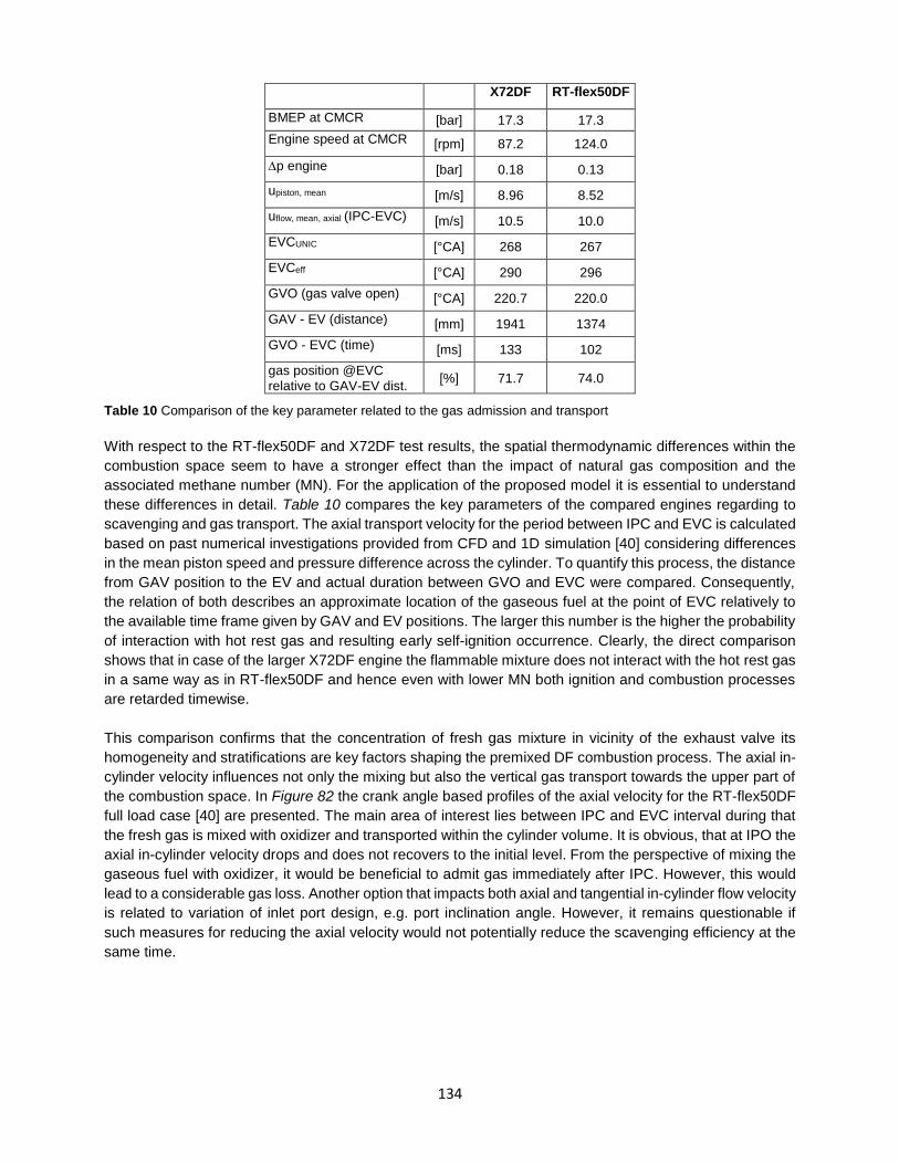
134
X72DF RT-flex50DF
BMEP at CMCR [bar] 17.3 17.3
Engine speed at CMCR [rpm] 87.2 124.0
p engine [bar] 0.18 0.13
upiston, mean [m/s] 8.96 8.52
uflow, mean, axial (IPC-EVC) [m/s] 10.5 10.0
EVCUNIC [°CA] 268 267
EVCeff [°CA] 290 296
GVO (gas valve open) [°CA] 220.7 220.0
GAV - EV (distance) [mm] 1941 1374
GVO - EVC (time) [ms] 133 102
gas position @EVC relative to GAV-EV dist.
[%] 71.7 74.0
Table 10 Comparison of the key parameter related to the gas admission and transport
With respect to the RT-flex50DF and X72DF test results, the spatial thermodynamic differences within the
combustion space seem to have a stronger effect than the impact of natural gas composition and the
associated methane number (MN). For the application of the proposed model it is essential to understand
these differences in detail. Table 10 compares the key parameters of the compared engines regarding to
scavenging and gas transport. The axial transport velocity for the period between IPC and EVC is calculated
based on past numerical investigations provided from CFD and 1D simulation [40] considering differences
in the mean piston speed and pressure difference across the cylinder. To quantify this process, the distance
from GAV position to the EV and actual duration between GVO and EVC were compared. Consequently,
the relation of both describes an approximate location of the gaseous fuel at the point of EVC relatively to
the available time frame given by GAV and EV positions. The larger this number is the higher the probability
of interaction with hot rest gas and resulting early self-ignition occurrence. Clearly, the direct comparison
shows that in case of the larger X72DF engine the flammable mixture does not interact with the hot rest gas
in a same way as in RT-flex50DF and hence even with lower MN both ignition and combustion processes
are retarded timewise.
This comparison confirms that the concentration of fresh gas mixture in vicinity of the exhaust valve its
homogeneity and stratifications are key factors shaping the premixed DF combustion process. The axial in-
cylinder velocity influences not only the mixing but also the vertical gas transport towards the upper part of
the combustion space. In Figure 82 the crank angle based profiles of the axial velocity for the RT-flex50DF
full load case [40] are presented. The main area of interest lies between IPC and EVC interval during that
the fresh gas is mixed with oxidizer and transported within the cylinder volume. It is obvious, that at IPO the
axial in-cylinder velocity drops and does not recovers to the initial level. From the perspective of mixing the
gaseous fuel with oxidizer, it would be beneficial to admit gas immediately after IPC. However, this would
lead to a considerable gas loss. Another option that impacts both axial and tangential in-cylinder flow velocity
is related to variation of inlet port design, e.g. port inclination angle. However, it remains questionable if
such measures for reducing the axial velocity would not potentially reduce the scavenging efficiency at the
same time.
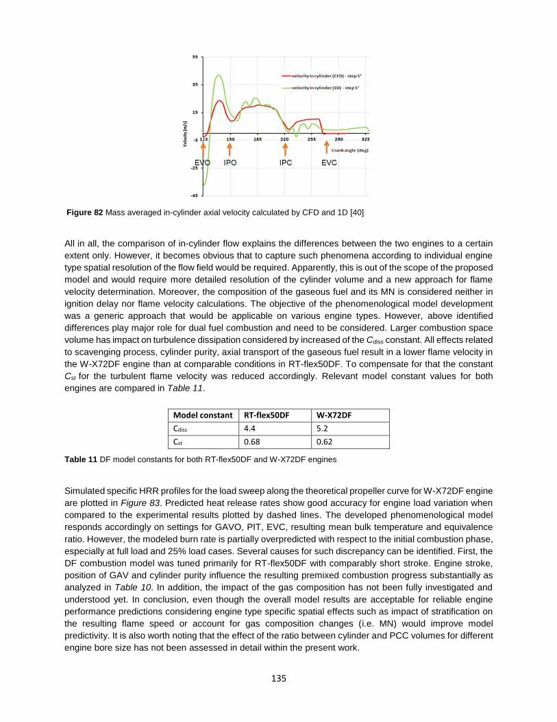
135
Figure 82 Mass averaged in-cylinder axial velocity calculated by CFD and 1D [40]
All in all, the comparison of in-cylinder flow explains the differences between the two engines to a certain
extent only. However, it becomes obvious that to capture such phenomena according to individual engine
type spatial resolution of the flow field would be required. Apparently, this is out of the scope of the proposed
model and would require more detailed resolution of the cylinder volume and a new approach for flame
velocity determination. Moreover, the composition of the gaseous fuel and its MN is considered neither in
ignition delay nor flame velocity calculations. The objective of the phenomenological model development
was a generic approach that would be applicable on various engine types. However, above identified
differences play major role for dual fuel combustion and need to be considered. Larger combustion space
volume has impact on turbulence dissipation considered by increased of the Cdiss constant. All effects related
to scavenging process, cylinder purity, axial transport of the gaseous fuel result in a lower flame velocity in
the W-X72DF engine than at comparable conditions in RT-flex50DF. To compensate for that the constant
Cst for the turbulent flame velocity was reduced accordingly. Relevant model constant values for both
engines are compared in Table 11.
Model constant RT-flex50DF W-X72DF
Cdiss 4.4 5.2
Cst 0.68 0.62
Table 11 DF model constants for both RT-flex50DF and W-X72DF engines
Simulated specific HRR profiles for the load sweep along the theoretical propeller curve for W-X72DF engine
are plotted in Figure 83. Predicted heat release rates show good accuracy for engine load variation when
compared to the experimental results plotted by dashed lines. The developed phenomenological model
responds accordingly on settings for GAVO, PIT, EVC, resulting mean bulk temperature and equivalence
ratio. However, the modeled burn rate is partially overpredicted with respect to the initial combustion phase,
especially at full load and 25% load cases. Several causes for such discrepancy can be identified. First, the
DF combustion model was tuned primarily for RT-flex50DF with comparably short stroke. Engine stroke,
position of GAV and cylinder purity influence the resulting premixed combustion progress substantially as
analyzed in Table 10. In addition, the impact of the gas composition has not been fully investigated and
understood yet. In conclusion, even though the overall model results are acceptable for reliable engine
performance predictions considering engine type specific spatial effects such as impact of stratification on
the resulting flame speed or account for gas composition changes (i.e. MN) would improve model
predictivity. It is also worth noting that the effect of the ratio between cylinder and PCC volumes for different
engine bore size has not been assessed in detail within the present work.
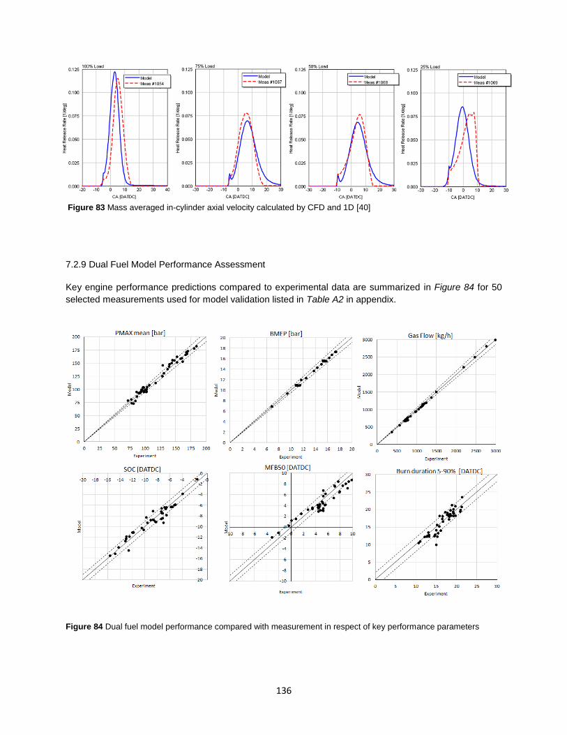
136
Figure 83 Mass averaged in-cylinder axial velocity calculated by CFD and 1D [40]
7.2.9 Dual Fuel Model Performance Assessment
Key engine performance predictions compared to experimental data are summarized in Figure 84 for 50
selected measurements used for model validation listed in Table A2 in appendix.
Figure 84 Dual fuel model performance compared with measurement in respect of key performance parameters
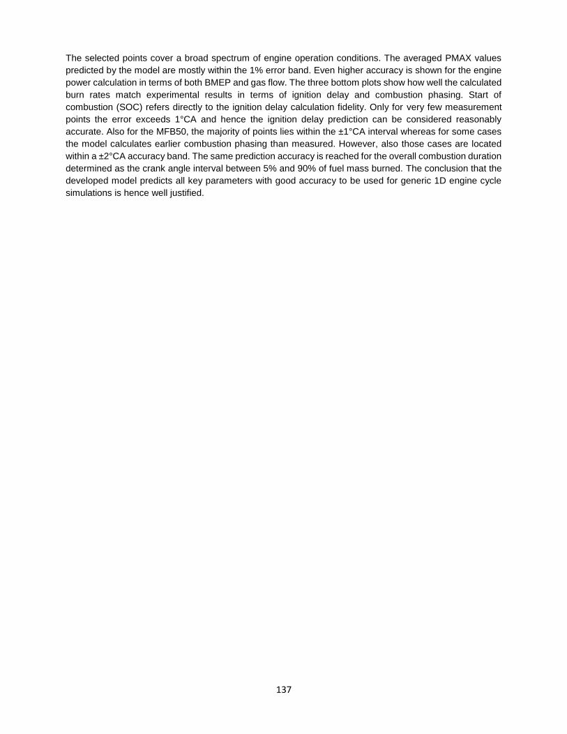
137
The selected points cover a broad spectrum of engine operation conditions. The averaged PMAX values
predicted by the model are mostly within the 1% error band. Even higher accuracy is shown for the engine
power calculation in terms of both BMEP and gas flow. The three bottom plots show how well the calculated
burn rates match experimental results in terms of ignition delay and combustion phasing. Start of
combustion (SOC) refers directly to the ignition delay calculation fidelity. Only for very few measurement
points the error exceeds 1°CA and hence the ignition delay prediction can be considered reasonably
accurate. Also for the MFB50, the majority of points lies within the ±1°CA interval whereas for some cases
the model calculates earlier combustion phasing than measured. However, also those cases are located
within a ±2°CA accuracy band. The same prediction accuracy is reached for the overall combustion duration
determined as the crank angle interval between 5% and 90% of fuel mass burned. The conclusion that the
developed model predicts all key parameters with good accuracy to be used for generic 1D engine cycle
simulations is hence well justified.

138
7.3 Model Applications
7.3.1 Integrated System Simulation
The proposed combustion simulation approach allows fast engine cycle simulation and analysis of a
complex propulsion systems. To demonstrate its capabilities, a methodology for an integrated system
simulation of engine, injector and exhaust valve system is defined using the developed predictive diesel
combustion model.
Combining various models into a one, the time demanding data transfer process often accompanied with
the necessary data conversion from one simulation environment to another can be avoided. Furthermore,
the generic character of each submodel allows utilization in the early phase of engine development when
the final tuning is unknown. For instance, the fuel rail-pressure or servo-oil pressure can be varied in a wide
range to assess the best combination for the targeted engine performance figures. In this respect, the
predictive combustion model introduces the key component of the system model to provide necessary
boundary conditions for other submodels.
Figure 85 Integrated system simulation layout combining engine cycle simulation with hydraulic injector and exhaust valve circuits.
Figure 85 outlines the layout of the coupled simulation incorporating the detailed engine model with mapped
turbocharger, exhaust valve drive circuit and detailed common-rail injector model. As highlighted on the plot
by set of labeled arrows, from the engine cycle simulation parameter signals for in-cylinder pressure,
injection timing, fuel rail-pressure or exhaust valve timing are passed to both injector and exhaust valve
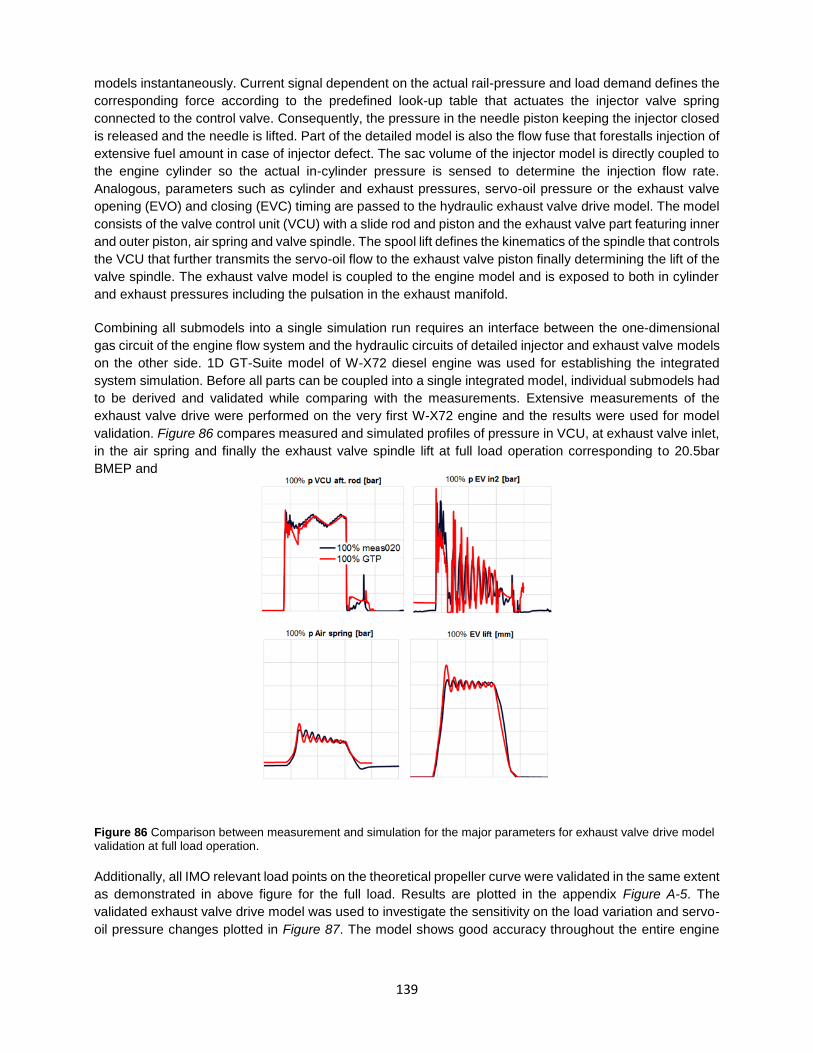
139
models instantaneously. Current signal dependent on the actual rail-pressure and load demand defines the
corresponding force according to the predefined look-up table that actuates the injector valve spring
connected to the control valve. Consequently, the pressure in the needle piston keeping the injector closed
is released and the needle is lifted. Part of the detailed model is also the flow fuse that forestalls injection of
extensive fuel amount in case of injector defect. The sac volume of the injector model is directly coupled to
the engine cylinder so the actual in-cylinder pressure is sensed to determine the injection flow rate.
Analogous, parameters such as cylinder and exhaust pressures, servo-oil pressure or the exhaust valve
opening (EVO) and closing (EVC) timing are passed to the hydraulic exhaust valve drive model. The model
consists of the valve control unit (VCU) with a slide rod and piston and the exhaust valve part featuring inner
and outer piston, air spring and valve spindle. The spool lift defines the kinematics of the spindle that controls
the VCU that further transmits the servo-oil flow to the exhaust valve piston finally determining the lift of the
valve spindle. The exhaust valve model is coupled to the engine model and is exposed to both in cylinder
and exhaust pressures including the pulsation in the exhaust manifold.
Combining all submodels into a single simulation run requires an interface between the one-dimensional
gas circuit of the engine flow system and the hydraulic circuits of detailed injector and exhaust valve models
on the other side. 1D GT-Suite model of W-X72 diesel engine was used for establishing the integrated
system simulation. Before all parts can be coupled into a single integrated model, individual submodels had
to be derived and validated while comparing with the measurements. Extensive measurements of the
exhaust valve drive were performed on the very first W-X72 engine and the results were used for model
validation. Figure 86 compares measured and simulated profiles of pressure in VCU, at exhaust valve inlet,
in the air spring and finally the exhaust valve spindle lift at full load operation corresponding to 20.5bar
BMEP and
Figure 86 Comparison between measurement and simulation for the major parameters for exhaust valve drive model validation at full load operation.
Additionally, all IMO relevant load points on the theoretical propeller curve were validated in the same extent
as demonstrated in above figure for the full load. Results are plotted in the appendix Figure A-5. The
validated exhaust valve drive model was used to investigate the sensitivity on the load variation and servo-
oil pressure changes plotted in Figure 87. The model shows good accuracy throughout the entire engine

140
load range and reflects changes in the servo-oil pressure by adapting the exhaust valve opening velocity
response correspondingly.
Figure 87 Simulated exhaust valve lift curves for engine load sweep (left) and servo-oil variations (right)
Unfortunately, no injector needle lift measurements were available to confirm the accuracy of the injector
model simulation. Nevertheless, the injection pressure above the needle tip was measured at four different
load points and compared with the simulation results in Figure 88. Immediately after the needle lift onset a
pressure drop is generated and followed by a recovery phase as the injection progresses. Both phenomena
are well represented by the model. Moreover, the oscillation frequency after end of injection (EOI) calculated
by the model matches well experimental data. However, no effect of multiple injectors is taken into account
in the hydraulic model since only a single injector is simulated. Therefore, the damping of pressure
oscillations is stronger based on simulation results than actually measured. However, such an effect has
only minor impact on the effective injection rate.
Figure 88 Injection pressure simulation (in red) compared with measurements (blue) for RT-flex60 engine load sweep
Since the time steps of hydraulic circuits are significantly smaller than for the gas circuit of the engine a model reduction is needed for optimizing the integrated run and reduce CPU time demand. Using an
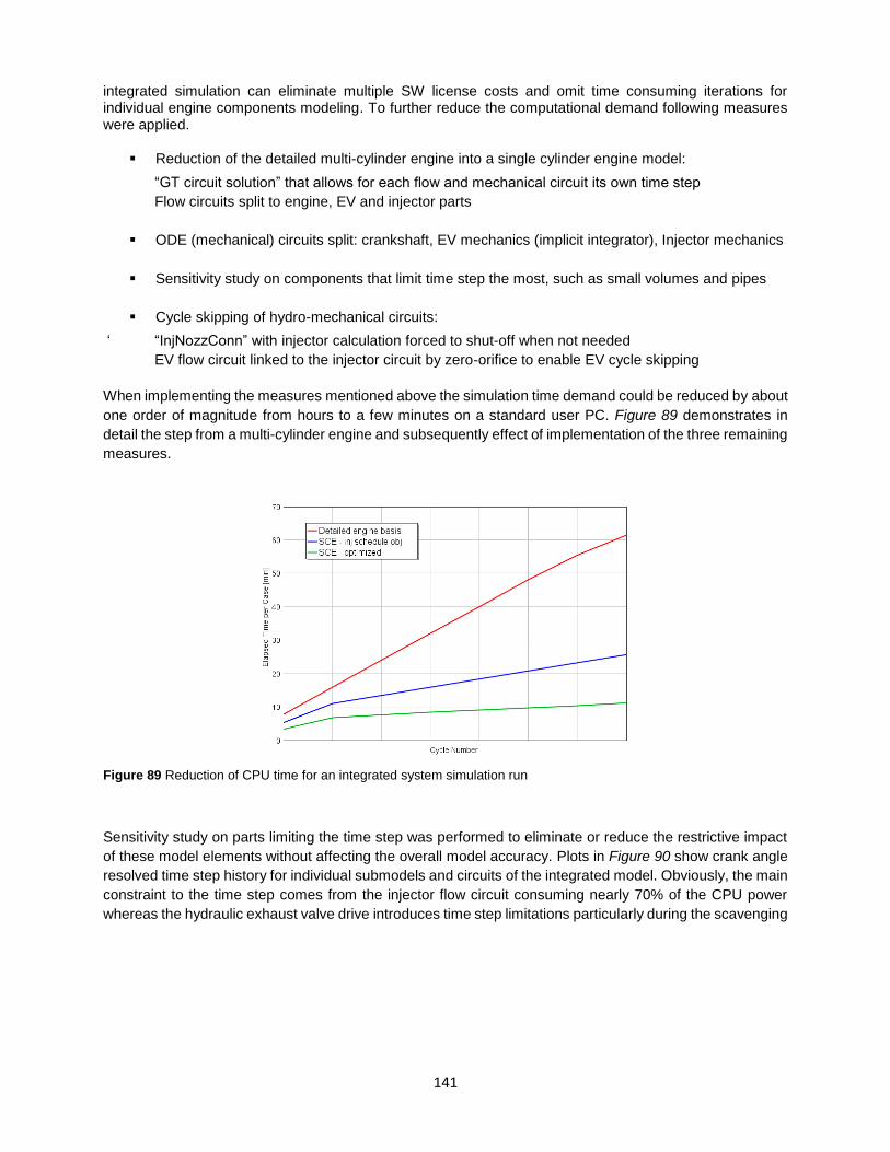
141
integrated simulation can eliminate multiple SW license costs and omit time consuming iterations for individual engine components modeling. To further reduce the computational demand following measures were applied.
▪ Reduction of the detailed multi-cylinder engine into a single cylinder engine model:
“GT circuit solution” that allows for each flow and mechanical circuit its own time step
Flow circuits split to engine, EV and injector parts
▪ ODE (mechanical) circuits split: crankshaft, EV mechanics (implicit integrator), Injector mechanics
▪ Sensitivity study on components that limit time step the most, such as small volumes and pipes
▪ Cycle skipping of hydro-mechanical circuits:
‘ “InjNozzConn” with injector calculation forced to shut-off when not needed
EV flow circuit linked to the injector circuit by zero-orifice to enable EV cycle skipping
When implementing the measures mentioned above the simulation time demand could be reduced by about
one order of magnitude from hours to a few minutes on a standard user PC. Figure 89 demonstrates in
detail the step from a multi-cylinder engine and subsequently effect of implementation of the three remaining
measures.
Figure 89 Reduction of CPU time for an integrated system simulation run
Sensitivity study on parts limiting the time step was performed to eliminate or reduce the restrictive impact
of these model elements without affecting the overall model accuracy. Plots in Figure 90 show crank angle
resolved time step history for individual submodels and circuits of the integrated model. Obviously, the main
constraint to the time step comes from the injector flow circuit consuming nearly 70% of the CPU power
whereas the hydraulic exhaust valve drive introduces time step limitations particularly during the scavenging
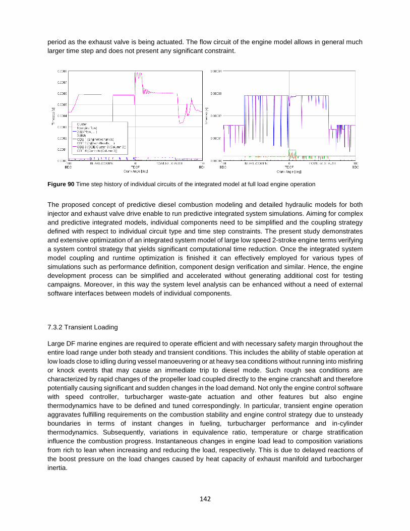
142
period as the exhaust valve is being actuated. The flow circuit of the engine model allows in general much
larger time step and does not present any significant constraint.
Figure 90 Time step history of individual circuits of the integrated model at full load engine operation
The proposed concept of predictive diesel combustion modeling and detailed hydraulic models for both
injector and exhaust valve drive enable to run predictive integrated system simulations. Aiming for complex
and predictive integrated models, individual components need to be simplified and the coupling strategy
defined with respect to individual circuit type and time step constraints. The present study demonstrates
and extensive optimization of an integrated system model of large low speed 2-stroke engine terms verifying
a system control strategy that yields significant computational time reduction. Once the integrated system
model coupling and runtime optimization is finished it can effectively employed for various types of
simulations such as performance definition, component design verification and similar. Hence, the engine
development process can be simplified and accelerated without generating additional cost for testing
campaigns. Moreover, in this way the system level analysis can be enhanced without a need of external
software interfaces between models of individual components.
7.3.2 Transient Loading
Large DF marine engines are required to operate efficient and with necessary safety margin throughout the
entire load range under both steady and transient conditions. This includes the ability of stable operation at
low loads close to idling during vessel manoeuvering or at heavy sea conditions without running into misfiring
or knock events that may cause an immediate trip to diesel mode. Such rough sea conditions are
characterized by rapid changes of the propeller load coupled directly to the engine crancshaft and therefore
potentially causing significant and sudden changes in the load demand. Not only the engine control software
with speed controller, turbucharger waste-gate actuation and other features but also engine
thermodynamics have to be defined and tuned correspondingly. In particular, transient engine operation
aggravates fulfilling requirements on the combustion stability and engine control strategy due to unsteady
boundaries in terms of instant changes in fueling, turbucharger performance and in-cylinder
thermodynamics. Subsequently, variations in equivalence ratio, temperature or charge stratification
influence the combustion progress. Instantaneous changes in engine load lead to composition variations
from rich to lean when increasing and reducing the load, respectively. This is due to delayed reactions of
the boost pressure on the load changes caused by heat capacity of exhaust manifold and turbocharger
inertia.

143
In order to validate the capability of the large DF engine to operate under transient conditions several test
have been performed on the RT-flex50DF test engine. The heavy sea conditions were simulated by
continuos changes in engine speed or load demand. Figure 91 shows an expample of experimental test
results wirth respect to engine load and speed response on brake load variation. With the introduction of
predictive DF combustion model in Section 6, heat release rate response on in-cylinder conditions such as
temperature, pressure or equivalence ratio can be captured accordingly. The proposed model was
succesfully validated under steady state operation for variations of numerous parameters. Application of the
fast running model for transient engine loading analysis has pontential to support the development process
and reduce the required testing demand. Furthermore, using integration in a 1D engine cycle environment,
optimum engine performance settings or turbocharging strategy for EWG control.
Figure 91 Measured engine response for wave loading conditions [96] used as an input for transient simulation
To validate the transient performance of the DF combustion model wave loading test was simulated
according to a real measurement. The experimental data were obtained from the RT-flex50DF test engine
at 85% load corresponding to 6550kW with 600kW variation in engine power. This variation was generated
by instant load changes on the water brake whereas the target engine speed setpoint was governded by
the speed controller. Detailed 1D multi-cylinder engine model including measurement based turbocharger
maps and integrated combustion model was utilized to recalculate the wave loading test. Since no speed
controller was implemented into the simulation model, except for the instantaneous load changes also the
engine speed temporal variation was imposed as an model input. Both engine power and speed variations
were replaced by a sinus based function according to the measured profile meeting the frequency and
deflections from the mean as presented in Figure 91.
Dual fuel model calculation was initialized at conditions relevant for steady state operation at 85% engine
load. Subsequently, 230s transient engine operation was simulated. Figure 92 shows both mesured and
simulated profiles the key monitored performance figures. It is worth noting that the curve representing
engine power is calculated from the IMEP averaged for all 6 cylinders. Hence, the apparent oscillations are
related to cyclic variations and do not correspond to the real measured engine brake power. Upper two plots
define instantaneous model inputs for engine power and speed aproximated by a sinusoid according to the
measured profiles. Below, prediction of combustion phasing MFB50 and cycle maximum cylinder pressure
PMAX is plotted and compared with measurements. With respect to combustion phasing the model
reproduces well the changing HRR due to variation of engine load and equivalence ratio assosiated with
scavenging pressure variation. Similarly, the calculated cycle maximum cylinder pressure corresonds to the
measured values averaged over all 6 cylinders. The phase shift of individual waves is related to the
irregularity of the measured loading that was imposed manually. Moreover, the predicted maximum peak
firing pressures are for the cycles at maxium engine load slightly underpredicted. Since the predicted
combustion phasing for the load peaks matches well with measurement, the difference is mainly related to

144
improper simulation of transient turbocharger performance. Also cycles at the minimum engine load are not
fully captured by the model in terms of combustion phasing and firing pressure. Nevertheless, both general
trend and magnitude of predicted figures confirms the generic validity of the proposed combustion simulation
also under transient conditions.
Figure 92 Transient wave loading for RT-flex50DF at 85% average load. Results of 1D cycle simulation using developed
DF combustion model are compared with measurements. Upper two plots show model inputs in terms of engine power
and speed adjusted to measured profiles. Lower plots illustrate model prediction in terms of MFB50 combustion phasin
and maximum cylinder pressure.
Cyclic resolved cylinder pressure history and HRR profiles calculated by the model for the prescribed load
and speed variations are plotted in the Figure 93. Additionally, black dashed lines from left to right

145
correspond to the heat release rates calculated from the cylinder pressure analysis for maximum, mean and
minimum engine power, respectively. All experimental profiles are averaged over 6 cylinders for a single
cycle. The model shows good prediction accuracy in terms of the mean HRR and cylinder pressure history.
For the limit cases representing the maximum and minimum of the imposed load profile the calculated HRR,
in terms of both onset (SOC) and shape, was underpredicted and overpredicted, respectively. In a similar
way, the simulated cylinder pressure curves match well the average but the limit cycles lie outside of the
range coverd by the model. Based on these observations it can be concluded that the stochastic character
of premixed turbulent combustion cannot be fully captured by a model linked to the mean in-cylinder
properties such as temperature and concentrations distribution. Effects related to spatial differences in
unburned and burned gas distribution, end gas knock or uncomplete combustion at lean conditions lead to
cyclic deviations in the HRR progress and affect the combustion stability. Such effects have impact on both
ignition delay and flame front propagation of maximum and minimum cycles demonstrated in Figure 93.
Figure 93 Cycle resolved HRR and cylinder pressure curves for wave loading at 85% compared to measurements for
maximum, mean and minimum engine power.
Engine load variations directly impact the turbocharger operation due to the induced changes in the exhaust
gas enthalpy. Shifting the turbocharger operating point determines the actual scavenging pressure and so
influences in-cylinder compression pressure, temperature of unburned gas-air mixture as well as trapped
equivalence ratio. These changes then govern the model calculation of ignition delay and heat release rates.
Apparently, there is a tight relationship between the DF combustion behavior and turbocharger performance.
For the present transient wave loading the turbocharger speed and mass averaged efficiencies for both
turbine and compressor are plotted in Figure 94. The corresponding compressor efficiency map is illustrated
in Figure 95 with indication of instantaneous operation trajectory by a black curve and an averaged operation
point represented by a blue point. It needs to be mentioned that the presented wave loading experiment
was run with the initial turbocharger match that was not ideal especially at high load operation. Within the
development progress, a suitable turbocharger match was employed introducing substantial improvement
of turbine efficiency and enhancement of compressor surge margin. In general, transient application of the
developed phenomenological combustion model shows further benefits for propulsion system optimization
in terms of turbocharger matching under both steady state and transient operation

146
Figure 94 Turbocharger speed and efficiency during transient wave loading at 85% load
Figure 95 Compressor efficiency map for the transient wave loading at 85% load
In conclusion, the application of the DF combustion model integrated into 1D engine cycle simulation tool
has proven the viability of the proposed modeling concept under transient operating conditions. Both
combustion process and engine performance can be predicted with good accuracy. A particularly important
feature of any modeling efforts at the early stage of engine development process is the engine design
definition. In this respect the model transient capability allows its application for investigation of the impact
of cyclic variations on the engine structure. This includes maximum allowed in-cylinder pressure, torsional
vibration analysis or main bearings layout associated with the lubrication and wear.

147
8. Conclusions
Following the thesis objectives phenomenological aspects of combustion in large low speed 2-stroke marine
engines with respect to both diesel and dual fuel combustion were thoroughly assessed on the basis of
results of extensive experimental investigations as well as detailed CFD simulations. The key findings from
this assessment were employed for developing models describing combustion phenomenology on the basis
of various submodels relevant to spray morphology, mixture formation, ignition delay, turbulence, spray
interactions or premixed flame velocity. These submodels were first individually validated against
experimental data or dedicated computational studies and the resulting complete models then integrated in
the form of user combustion routine in a commercial 1D engine cycle simulation tool. Final model calibration
was done by comparing the predicted heat release data with real engine results. Regarding key performance
figures, the modeling methodology has shown good level of accuracy and predictivity.
The state of the art study has revealed that in spite of numerous models available especially for diesel
combustion there is a gap in terms of fast and predictive combustion models in the segment of large 2-stoke
marine engines. This gap is even larger for lean burn DF combustion in such engines with direct low
pressure gas admission and pre-chamber pilot fuel ignition, which could previously not be simulated at all
in a fast and predictive way due to the lack of any suitable phenomenological approach. This is due to the
complexity of the combustion systems involved, which is associated with the presence of multiple peripheral
injectors in the diesel case and the deviation from stoichiometric and homogeneous mixture composition in
the DF case. In order to formulate a generic modeling concept, a quasi-dimensional approach was identified
as prerequisite to account for spatially resolved phenomena such as interactions of diesel sprays or ignition
delay of premixed charge. Therefore, the proposed simulation methodology represents a novel approach
for fast running physics based models for diesel and dual fuel combustion regimes applicable in such
engines.
Within the diesel combustion model both zero-dimensional turbulence and quasi-dimensional spray
interaction models are essential with respect to overall model accuracy. The spray formation and interaction
model was developed adopting results of elementary spray research carried out in the spray combustion
chamber (SCC) and multidimensional CFD simulations. Individual submodels for spray penetration,
dispersion and ignition delay were validated against experiments. For consistency purpose, these
submodels were not further adjusted for optimization of the predicted HRR. The spray interaction model is
based on quasi-dimensional resolution of spray penetration within the combustion space and the amount of
fuel available for the diffusive combustion is related to the ratio of free and interacted spray area. Both
premixed and diffusion combustion models were derived adopting the time scale approach. Corresponding
model constants were tuned primarily with respect to experimental heat release rate measured on the RT-
flex60 engine for load and key parameter variations.
Ignition delay predictions are in very good agreement with start of combustion observations for the engine
cases simulated. Note that, for the large low speed 2-stroke engine the premixed combustion phase is
mostly negligible. Hence, the transition between both combustion regimes cannot be assessed in detail.
Nonetheless, single cases at reduced compression ratio confirm the validity of the resulting heat release
rate patterns in view of the adequate premixed peak predictions. The spray interaction onset is well captured
by the model and corresponds with the measured start of the HRR restriction due to local lack of oxidizer.
Likewise, the HRR recovery phase and the associated acceleration of the heat release rate is predicted in
line with measurements, even if model application to other engine types yielded somewhat advanced onset
148
of spray interactions and partial overprediction of the HRR recovery phase. The sensitivity study covering a
broad variation of engine parameters confirmed the generic character of the developed mode. High quality
of HRR and engine performance predictions was achieved for load and fuel rail pressure variations.
However, nozzle execution specific differences can be captured only by trend but not in terms of exact spray
interaction magnitude and late combustion phase progress. Similarly, predictions for the implemented
sequential injection strategy were not sufficiently accurate. Except for such very special cases, the results
of key engine performance figures and combustion phasing predictions are very good and the approach
hence meets the requirements for fast and predictive engine cycle simulations.
Analogously, the DF model is strongly dependent on the appropriate description of turbulence-chemistry
interaction effects as well as the proper representation of quasi-dimensional aspects associated with the
deviation from homogeneity of the premixed charge and the associated impact on ignition. The model was
derived by applying premixed and turbulent flame theory to the present case of a large low speed engine.
Due to the limited experimental database directly meeting requirements of large 2-stroke marine engines,
literature research and detailed kinetic models were utilized for model derivation. Individual submodels were
validated against results of multi-dimensional CFD investigations. Ignition delay was modeled for both pilot
diesel injection and the gaseous fuel. The latter relates closely to the scavenging and gas admission process
that take place simultaneously. Here, a cylinder discretization was proposed to allow for spatial differences
in burn gas concentrations, temperature and the equivalences ratio of the gas-air mixture. Subsequently,
the locally resolved conditions are utilized for determining the auto-ignition of the gaseous fuel substituted
by methane in present study.
Predictions made my means of this model are well in line with experimental observations made in the context
of extensive parametric variations conducted on a test engine. By nature, deviations are somewhat larger
than for the diesel model but computed ignition delay is in good agreement with start of combustion
detections on the engine. The same applies for the HRR progress parameters investigated, even if, for some
cases, the model tends to predict slightly faster combustion than observed in the tests. Nonetheless, the
conclusion that the developed model predicts all key parameters with sufficient accuracy to be used for
generic 1D engine cycle simulations is well justified.
The relevance of an appropriate representation of turbulence for both models cannot be overemphasized.
Reducing the k- turbulence model to a zero-dimensional form for isotropic and homogeneous turbulence
has proven successful as was demonstrated by the quality of the predicted mean cylinder TKE. TKE is
decisive in terms of diffusion combustion prediction as well as turbulent flame velocity determination.
Therefore, the relevant turbulence generation effects need to be properly accounted for, including the flow
through the inlet ports, gas admission for the DF as well as fuel injection for the diesel case. In this respect
the initial fuel injection rate profile together with the effective injection pressure need to be properly defined.
There are several features and general limitations of proposed methodology for combustion modeling that
are worth noting. By nature, the pronounced fidelity compromise compared to multidimensional CFD models
is indisputable. With respect to the reduced zero-dimensional turbulence model, the limited prediction
accuracy showed negligible impact on simulated heat release rate. On the other hand, the lack of spatial
resolution has a direct impact on both ignition delay and flame speed computation. Concerning the generic
validity, in contrast to the author’s intention to do without artificial model constants, the application to different
engines types and bore sizes requires yet some model adaptations. This is prerequisite for both diesel and
dual models due to differences in ignition behavior, turbulence generation and dissipation or spray
interactions related to injector number or in-cylinder flow. Especially the application of the spray interaction
model on various engines types has unveiled several deficiencies linked to the quasi-dimensional model.
With respect to the DF combustion model, the model at present cannot predict knock and neglects the
impact of gas quality (MN) on flame propagation. Furthermore, the validity of emission predictions in terms

149
of nitric oxide and soot formation could not be confirmed due to the limited scope of the present work.
Nevertheless, corresponding models were outlined and can be easily implemented within the user code
structure and subsequently integrated in the 1D simulation tool.
The integration of the models into the GT-Suite simulation environment has proven the feasibility of the
proposed methodology to be effectively used for fast engine cycle studies of multiple cases or extensive
DoE runs. Thanks to the generic character of the combustion model this can be done already in the early
phases of a development process. The simulation methodology developed in the present thesis has been
successfully demonstrated on a variety of 1D fast running models and has been published and well accepted
at SAE World Congress 2016 [20] and Gamma Technologies user’s conference [19]. Moreover, case
studies using the proposed methodology for combustion simulation have demonstrated the potential of the
developed modeling approach for industry applications and we envisage the application of the proposed
simulation methodology for optimizing actual large 2-stroke engines and integrated marine propulsion
systems. There are several features and general limitations of proposed methodology of combustion
modeling that are worth noting. Fidelity compromise compared to multidimensional CFD
____________________________________________________________________________________
___________________
______________

150
Acknowledgments
The present thesis was elaborated in the combined form of doctoral studies in parallel with my work at
Wärtsilä Switzerland Ltd. and completed while employed at GE Global Research Munich. Experimental
investigations were carried out mainly during my stays at Wärtsilä Italia S.p.A in Trieste, Italy and at Diesel
United Ltd. in Aioi, Japan. Further experimental data were adopted from Wärtsilä research facility in
Winterthur, Switzerland.
First of all, I would like to thank Prof. J. Macek for his outstanding support, academic guidance, many
valuable and motivating discussions and giving me the opportuning to complete my thesis parallel to my
work assignments.
Special thanks to Dr. G. Weisser who promoted my interest in combustion simulation of large marine
engines, provided me a pleasant working environment, guided my work and for his willingness to act as co-
examiner.
Furthermore, I am grateful to my colleagues at Wärtsilä for their support in terms of numerical simulations,
providing me experimental data, participation in my research project and through valuable discussions, in
particular Prof. K. Herrmann, Dr. S. Hensel, Dr. P. Rebecchi, Dr. R. Schultz, Dr. B. von Rotz, C. Hattar, M.
Ott, Y. Jia and M. Grasso.
Additional recognition belongs to K. Moriyama for organizing my stay at Diesel United Ltd. Aioi, Japan
Last but not least, I would also like to thank to my parents for their continuous support and trust allowing me
to concentrate on my studies and research work.

151
______________________________________________
References
1 Abdel-Gayed, R. G., Bradley, D., Lawes, M., “Turbulent burning velocities: A general correlation in terms of strain rates”, Proc. Roy. Soc. Lond. A414, p. 389–413, 1987.
2 Andrews, G. E., Bradley, D., “The burning velocity of methane–air mixtures”, Combustion and Flame, 19, p. 275–288, 1972.
3 Annand, W. J. D., “Heat Transfer in the Cylinder of Reciprocating Internal Combustion Engines”, Proc Instn Mech Engrs, Vol. 177, p. 973-990, 1963.
4 Assanis, D.N., Filipi, Z.S., Fiveland, S.B. , Syrimis, M., "A Predictive Ignition Delay Correlation Under Steady-State and Transient Operation of a Direct Injection Diesel Engine," Journal of Engineering for Gas Turbines and Power, 125(2), p. 450, 2003.
5 Austen, A. E. W.; Lyn, W. T., “Some Steps Toward Calculation Diesel Engine Behavior”, SAE-Paper 409A, 1961.
6 Barba, Ch.,“Erarbeitung von Verbrennungskennwerten aus Indizierdaten zur verbesserten Prognose und rechnerischen Simulation des Verbrennungsablaufes bei Pkw-DE-Dieselmotoren mit Common-Rail-Einspritzung“, Dissertation No. 14276, ETH Zürich, 2001.
7 Bargende, M. et al. „Turbulenzmodellierung für quasi-dimensionale Arbeitsprozessrechnung“, FVV Informations-tagung Motoren, 2014.
8 Bédat, B., Cheng, R. K., “Experimental Study of Premixed Flames in Intense Isotropic Turbulence”, Combustion and Flame, vol. 100, p485-494, 1995.
9 Blizard, N., Keck, C., “Experimental and Theoretical Investigation of Turbulent Burning Model for Internal Combustion Engines”, SAE Technical Paper 740191, 1974.
10 Borghi, R., “On the structure and Morphology of Turbulent Premixed Flames”, Recent Advances in Aeronautical Science, Plenum Press, New York, 1985.
11 Borghi, R., “Turbulent Combustion Modelling”, Progress in Energy and Combustion Science, Vol. 14, p. 245-292, 1988.
12 Boulouchos K., Eberle M. K., Ineichen B., Klukowski C., “New Insights into the Mechanisms of In-Cylinder Heat Transfer in Diesel Engines”, SAE Technical Paper 890573, 1989.
13 Boulouchos K., Isch R., “Modeling of Heat Transfer during Combustion: A Quasi-Dimensional Approach with Emphasis on Large Low-Speed Diesel Engines”, 1990.
14 Boulouchos K., Steiner T., “On the Relative Roles of Convective and Radiative Heat Transfer in Diesel Egines: The Effects of Size and Operating Conditions”, Eurotherm No. 15, IFM Toulouse, 1991.
15 Boussinesq, J.,”Théorie de l'écoulement tourbillonnant et tumultueux des liquides dans les lits rectilignes a grande section”, 1. Gauthier-Villars, Paris, 1897.
16 Bradley, D., “Fundamentals of Lean Combustion”, Lean Combustion Technology and Control, Elsevier, 2008.
17 Bradley, D., Gaskell, P.H., Gu, X. J., “Burning Velocities, Markstein Lengths and Flame Quenching for Spherical Methane-Air Flames: A Computational Study”, Combustion and Flame, vol.104, p.176-198, 1996.
18 Bradley, D., Lau, K-C., Lawes, M., “Flame stretch rate as a determinant of turbulent burning velocity”, Philosophical Transaction of the Royal Society of London A, vol. 338, p. 359-387, 1992.
19 Cernik, F., “Integrated 1D Simulation for a Large Low-Speed 2-Stroke Marine Engine”, Proceedings GT-Suite Users Conference, 2015. https://www.gtisoft.com/wp-content/uploads/2015/11/Integrated_1D_Simulation.pdf
20 Cernik, F., Macek, J., Dahnz, C., and Hensel, S., "Dual Fuel Combustion Model for a Large Low-Speed 2-Stroke Engine," SAE Technical Paper 2016-01-0770, 2016.
21 Chmela, F., Orthaber, G. C., “Rate of Heat Release Prediction for Direct Injection Diesel Engines Based on Purely Mixing Controlled Combustion”, SAE Paper 1999-01-0186, 1999.
22 Chmela, F.; Orthaber, G.; Schuster, W., „Die Vorausberechnung des Brennverlaufs von Dieselmotoren mit direkter Einspritzung auf der Basis des Einspritzverlaufs“, MTZ 59, Nr. 7/8, P. 484-492, 1998.

152
23 Damköhler, G., „Der Einfluß der Turbulenz auf die Flammengeschwindigkeit in Gasgemischen“, Zeitschrift für Elektrochemie und angewandte physikalische Chemie, Vol. 46, p.601-652, 1940.
24 De Bellis, V., Bozza, F., Fontanesi, S., Severi, E. et al., "Development of a Phenomenological Turbulence Model through a Hierarchical 1D/3D Approach Applied to a VVA Turbocharged Engine," SAE Int. J. Engines 9(1): p. 506-519, 2016.
25 Dec, J., “A Conceptual Model of DI Diesel Combustion Based on Laser-Sheet Imaging”, SAE Technical Paper 970873, 1997.
26 Dent, J., "A Basis for the Comparison of Various Experimental Methods for Studying Spray Penetration," SAE Technical Paper 710571, 1971.
27 Dinkelacker, F., Manickam, B., Muppala, S.P.R., “Modelling and simulation of lean premixed turbulent methane/hydrogen/air flame with an effective Lewis number approach”, Combustion and Flame, vol. 158, p1742-1749, 2011.
28 Divis, M., Macek, J., “Fuel Injection Process Computations Using the Eulerian Multidimensional Model”, ," SAE Technical Paper 2005-01-1243, 2006.
29 Dulbecco, A., Lafossas, F. A., Poinsot, T. J., “A 0D Phenomenological Approach to Model Diesel HCCI Combustion with Multi-Injection Strategies Using Probability Density Functions and Detailed Tabulated Chemistry”, SAE Paper 2009-01-0678, 2009.
30 Eilts, P., „Modell zur Vorausberechnung des Brenngesetzes mittelschnelllaufender Dieselmotoren“, MTZ 54, Nr.3, p.134-140, 1993.
31 Emani, B., Liu, R., Ting, D.S.K., Checkel, D., “A Numerical Study on the Burning Velocity of a Spherical, Premixed Methane-Air Flame”, SAE Technical Paper 2005-01-1124, 2005.
32 Faeth, G. M., Hsiang L.P., Wu, P.K., “Structure and Breakup Properties of Sprays”, International Journal Muliphase Flow Vol. 21, p. 99-127, 1995.
33 Faeth, G.M., “Current Status on Droplet and Liquid Combustion”, Progress in Energy and Combustion Science 3, p. 191-224, 1977.
34 Fenimore, C. P., “Formation of Nitric Oxide in Premixed Hydrocarbon Flames”, 13th Symp. Int. Combust., p. 373-379, 1971.
35 Gao X., Chen J., Ye Z., Foster D., Borman G. L., “Ignition delay and heat release analysis of an ethanol fumigated turbocharged diesel engine”, ASME Paper No 83-DGP-1, 1983.
36 Grill, M., Bargende, M., Rether, D., Schmid, A., “Quasi-dimensional and Empirical Modeling of Compression-Ignition Engine Combustion and Emissions. SAE Paper 2010-01-0151, 2010.
37 Grill, M., Billinger, T., and Bargende, M., "Quasi-Dimensional Modeling of Spark Ignition Engine Combustion with Variable Valve Train," SAE Technical Paper 2006-01-1107, 2006.
38 Gu, X. J., Haq, M. Z., Lawes, M., Woolley, R., “Laminar burning velocity and Markstein lengths of methane-air mixtures”, Combustion and Flame, vol.121, p. 41-58, 2000.
39 Gülder, Ö. L., “Turbulent Premixed Flame Propagation Models for Different Combustion Regimes”, 23rd Symposium (International) on Combustion, The Combustion Institute, p. 743-750,1990.
40 Halámek, M., “Model vyplachování dvoudobého pomaloběžného motoru spalujícího plynné palivo”, Diploma thesis, CTU Prague, 2013.
41 Halstead, M. P., Kirsch, L. J., Quinn, C. P., “The autoignition of hydrocarbon fuels at high temperatures and pressures – fitting of a mathematical model”, Combustion and Flame, 30, p. 45-60, 1977.
42 Hanson, R. K., Salimian, S., “Survey of Rate Constants in H/N/O Systems”, In W. C. Gardiner, editor, Combustion Chemistry, page 361, 1984.
43 Hardy, G., “RTX-4 CFD Combustion”, Technical Report, Wärtsilä Switzerland Ltd., 2010.
44 Hassan, M.I., Aung, K.T., Faeth, G.M., “Measured and predicted properties of laminar premixed methane/air flames at various pressures”, Combustion and Flame, vol. 115, p. 539–550, 1998.
45 Herrmann, K., von Rotz, B., Schulz, R., Weisser, G. et al., “Reference Data Generation of Spray Characteristics in Relation to Large 2-Stroke Marine Diesel Engines Using a Novel Spray Combustion Chamber Concept”, ILASS-Europe 2010, Czech Repuplic, 2010.
46 Hiroyasu, H., “Diesel Engine Combustion and Its Modeling”, International Symposium COMODIA 94, Japan, 1994.

153
47 Hiroyasu, H., Arai, M., “Structures of Fuel Sprays in Diesel Engines”, SAE Technical Paper 900475, 1990.
48 Hiroyasu, H., Kadota, T. , Arai, M., "Development and Use of a Spray Combustion Modeling to Predict Diesel Engine Efficiency and Pollutant Emissions: Part 2 Computational Procedure and Parametric Study",Bulletin of JSME 26(214), p. 576-583, 1983.
49 Hiroyasu, H., Kadota, T., “Models for Combustion and Formation of Nitric Oxide and Soot in Direct Injection Diesel Engines”, SAE-Paper 760129, 1976.
50 Hiroyasu, T., Miki, M., Kim, M., Watanabe, S., Hiroyasu, H., Miao, H., “Reduction of Heavy Duty Diesel Engine Emission and Fuel Economy with Multi-Objective Genetic Algorithm and Phenomenological Model”, SAE Paper 2004-01-0531, 2004.
51 Hountalas D. T., Papagiannakis, R. G., “Development of a Simulation Model for Direct Injection Dual Fuel Diesel-Natural Gas Engines”, SAE Technical Paper 2000-01-0286, 2000.
52 Imahashi, T., Tomita, E., Yoshiyama, S., Ichimura,S., Moriyama,K., “Estimation of Combustion Process Based on Rate of Heat Release Curve in a Two-Stroke Slow-Speed Large Marine Diesel Engine”, Cimac Congress 2004, Kyoto, Paper No. 121, 2004.
53 Imanishi, H., Yoshizaki, T., Hiroyasu, H., “Simulation Study of Effects of Injection Rate Profile and Air Entrainment Characteristics on D.I. Diesel Combustion”, SAE Paper 962059, 1996.
54 Inagaki, K., Ueda, M., Mizuta, J., Nakakita, K., Nakayama, S., “Universal Diesel Engine Simulator (UniDES):1st Report: Phenomenological Multi-Zone PDF Model for Predicting the Transient Behavior of Diesel Engine Combustion”, SAE Paper 2008-01-0843, 2008.
55 International Maritime Organization, “Annex VI of MARPOL 73/78: Regulations for the Prevention of Air Pollution from Ships and NOx Technical Code”, IMO-664E, London, 1998.
56 Johnson, S.L., Clarke, A., Fletcher, T., Hylands, D., “A Phenomenological Approach to Dual Fuel Combustion Modelling”, ASME, ICEF2012-92133, pp.781-791, 2012.
57 Jung, D., Assanis, D.N., “Multi-zone DI Diesel Spray Combustion Model for Cycle Simulation Studies of Engine Performance and Emissions”, SAE Paper 2001-01-1246, 2001.
58 Kadota, T., Hiroyasu, H., Oya, H., “Spontaneous Ignition Delay of a Fuel Droplet in High Pressure High Temperature Gaseous Environments,” Bull. JSME, 19(130), Paper No. 536.46, p. 437–445, 1976.
59 Kaufmann, D., „Vorausberechnung des Brennverlaufs bei langsamlaufenden Zweitakt-Grossdieselmotoren in Abhängigkeit von Betriebspunkt, Geometrie und Einspritzsystemkenngrössen“, Master thesis, ETH Zürich, 2006.
60 Khan, I. M., Greeves, G., Probert, D. M., “Air Pollution Control in Transport Engines”, Vol. C142/71, p. 205-217, The Institution of Mechanical Engineers, London, 1971.
61 Klimov, A. M., “Premixed turbulent flames - interplay of hydrodynamic and chemical phenomena”, AIAA Prog. Astronautics Aeronautics 88, 133-146, 1983.
62 Kobayashi, H., Kawabata, Y., Maruta, K., “Experimental Study on General Correlation of Turbulent Burning Velocity at High Pressure”, Proceedings of 27th Symposium (International) on Combustion, p. 941-948, 1998.
63 Kolade, B., Morel, T., Kong, S.-C., “Coupled 1-D/3-D Analysis of Fuel Injection and Diesel Engine Combustion”, SAE Paper 2004-01-0928, 2004.
64 Kolmogorov, A. N., “The local structure of turbulence in an incompressible viscous fluid for very large Reynolds numbers”, Dokl. Akad. Nauk SSSR 30, p. 301–305,1941.
65 Kong, S., Han, Z., Reitz, R.D., “The Development and Application of a Diesel Ignition and Combustion Model for Multidimensional Engine Simulation”, SAE Paper 950278, 1995.
66 Kono, S., Nagao, A. and Motoka, H., “Prediction of In-Cylinder Flow and Spray Formation Effects on Combustion in Direct Injection Diesel Engines,” SAE Paper 850108, 1985.
67 Kouremenos, D. A., Rakopoulos, C. D., and Hountalas, D.T., “Multi-Zone Combustion Modeling for the Prediction of Pollutants Emissions and Performance of DI Diesel Engines,” SAE Paper 970635, 1997.
68 Krenn, M., Redtenbacher, Ch., Pirker, G., Wimmer, A., „A new approach for combustion modeling of large dual-fuel engines“, 10th International MTZ Conference 2015 Heavy-Duty-, On- and Off-Highway Engines, 2015.
69 Krishnan, S. R., Srinivasan, K. K., Midkiff, K. C., “Modeling and Experiments of Dual-Fuel Engine Combustion and Emissions”, SAE Technical Paper 2007-01-0942, 2007.
154
70 Kuleshov, A. S., “Model for predicting air-fuel mixing, combustion and emissions in DI diesel engines over whole operating range”, SAE Paper 2005-01-2119, 2005
71 Kuleshov, A. S., “Multi-Zone DI Diesel Spray Combustion Model for Thermodynamic Simulation of Engine with PCCI and High EGR Level”, SAE Paper 2009-01-1956, 2009.
72 Kuleshov, A.S., Grekhov, L., “Multidimensional Optimization of DI Diesel Engine Process Using Multi-Zone Fuel Spray Combustion Model and Detailed Chemistry NOx Formation Model”, SAE Paper No 2013-01-0882, 2013.
73 Kyrtatos, P., Obrecht, P., Hoyer, K., Boulouchos, K., “Predictive Simulation and Experimental Validation of Phenomenological Combustion and Pollutant Models for Medium-Speed Common Rail Diesel Engines at Varying Inlet Conditions”, CIMAC Congress 2010, Bergen Paper No. 143, 2010.
74 Lämmle, Ch., “Numerical and Experimental Study of Flame Propagation and Knock in a Compressed Natural Gas Engine“, Dissertation No. 16362, ETZ Zürich, 2005.
75 Li, J., Che, J., Jeong, J., “Modeling the Effects of Split Injection Scheme on Soot and NO Emission of Direct Injection Diesel Engines by a Phenomenological Combustion Model”, SAE Paper 962062, 1996.
76 Liao, S. Y., Jiang, D.M., Cheng, Q., „Determination of laminar burning velocities for natural gas“, Fuel, p. 1247-1250, 2004.
77 Liu, Z., Karim, G.A., “Predictive Model for the Combustion Process in Dual Fuel Engines”, SAE Technical Paper 952435, 1995.
78 Macek, J., Steiner, T., “Advanced Multizone Multi-dimensional Models of Engine Thermaerodynamics”, Proceedings of 21st CIMAC International Congress on Combustion Engines, 1995.
79 Macek, J., Suk., B., “Spalovací motory I“, Skripta CVUT Praha 1993, ISBN 80-01-02085-1, 2003.
80 Macek, J., Vitek, O., Dolecek, V., Srinivasan, S., Tanner, F. X., “Improved Simulation of Transient Engine Operations at Unsteady Speed Combining 1-D and 3-D Modeling”, SAE Paper 2009-01-1109, 2009.
81 Magnussen, B. F., “On the Structure of Turbulence and a Generalized Eddy Dissipation Concept for Chemical Reactions in Turbulent Flow”, 19th AIAA Sc. meeting, St. Louis, USA, 1981.
82 Mauviot, G., Albrecht, A., Poinsot, T. J., “A New 0D Approach for Diesel Com-bustion Modeling Coupling Probability Density Function with Complex Chemistry”, SAE Paper 2006-01-3332, 2006.
83 Metghalchi, M., Keck, J. C., “Burning Velocities of Mixtures of Air with Methanol, Isooctane and Indolene at High Pressure and Temperature”, Combustion and Flame, vol. 48, p. 191-210, 1982.
84 Morel T., Keribar R., “Heat Radiation in D.I. Diesel Engines”, SAE Paper 860445, 1986.
85 Morel, T., Keribar, R., “A Model for Predicting Spatially and Time Resolved Convective Heat Transger in Bowl-in-Piston Combustion Chambers, SAE Paper 850204, 1985.
86 Morel, T.; Wahiduzzaman, S., “Modeling of Diesel Combustion and Emissions”, XXVI FISITA Congress, Praha, 1996.
87 Muppala, S. P. R., Aluri, N. K., Dinkelacker, F., Leipertz, A., “Development of an algebraic reaction rate closure for the numerical calculation of turbulent premixed methane, ethylene, and propane/air flames for pressures up to 1.0 MPa”, Combustion and Flame, vol.140, p. 275-266, 2005.
88 Naber, J. D., Siebers, D., “Effects of Gas Density and Vaporization on Penetration and Dispersion of Diesel Sprays”, SAE Paper 960034, 1996.
89 Nakagawa, H., Oda, Y., Kato, S., Nakashima, M., Tateishi M., „Fuel Spray Motion in Side Injection System for Diesel Engines“, COMODIA 90, p.281-286, 1990.
90 Neely, G., Sasaki, S., Huang, Y., Leet, J. et al., "New Diesel Emission Control Strategy to Meet US Tier 2 Emissions Regulations," SAE Technical Paper 2005-01-1091, 2005.
91 Nylund, I., Ott, M., “Development of a Dual Fuel technology for slow-speed engines”, CIMAC Congress 2013, Shanghai, Paper No. 284, 2013.
92 O’Rourke, P.J., “Collective Drop Effects in Vaporizing Liquid Sprays, PhD Thesis, Princeton, 1981.
93 Oberg, H.-J., “Die Darstellung des Brennverlaufes eines mittelschnelllaufenden Dieselmotors durch zwei überlagerte Vibe-Funktionen“, Dissertation, TU Braunschweig, 1976.
94 Ogami, Y., Kobayashi, H., “Laminar Burning Velocity of Stoichiometric CH4/air Premixed Flames at High-Pressure and High-Temperature”, JSME, Series B, 48, No. 3, 2005.

155
95 Ohnesorge, W., “Die Bildung von Tropfen an Düsen und Auflösung flüsiiger Strahlen, Z Angew Match Mech, vol. 16, p. 355, 1936.
96 Ott, M., Nylund, I., Alder, R., Yamada, T., Hirose, T., Umemoto. Y., “The 2-stroke low pressure Dual-Fuel technology: from concept to reality”, CIMAC Congress 2016, Helsinki, Paper No. 233, 2016.
97 Peters, N., “Laminar Flamelet Concepts in Turbulent Combustion”, Proceedings of 21th Symposium (International) on Combustion, p. 1231-1250, 1986.
98 Peters, N., “The turbulent burning velocity for large-scale and small scale turbulence”, Journal of Fluid Mechanics, vol. 384, p. 107-132, 1999.
99 Peters, N., “Turbulent Combustion”, Cambridge Univ. Press, Cambridge, UK, 2000.
100 Philipp, H., “Wärtsilä RTX-5 DF Combustion Visualization”, Technical Report, AVL, 2012.
101 Pirker, G., Chmela, F., Wimmer, A., “ROHR Simulation for DI Diesel Engines Based on Sequential Combustion Mechanisms”, SAE Paper 2006-01-0654, 2006.
102 Příhoda, J., Louda, P., “Matematické modelování turbulentního proudění“, Skripta CVUT Praha 2007, ISBN 978-80-01-03623-ř, 2007.
103 Reitz, R., D. et al., „WERC progress report on natural gas/diesel chemical kinetic mechanisms”, 2015.
104 Reitz, R.D., Bracco, F.V., “Mechanism of Breakup of Round Liquid Jets. Encyclopedia of Fluid Meachnics 3”, p. 233-249, 1986.
105 Rether D., Schmid A., Grill M., Bargende M.,“Quasidimensionale Simulation der Dieselverbrennung mit Vor- und Nacheinspritzung“, MTZ 71, Nr.10, S.742-748, 2010.
106 Rozenchan, G., Zhu, D.L., Law, C. K., Tse, S.D., “Outward propagation, burning velocities, and chemical effects of methane flames up to 60atm”, Proceedings of the Combustion Institute, vol. 29, p. 1461-1469, 2002.
107 Schreiner, K., „Der Polygon-Hyperbel-Ersatzbrennverlauf: Untersuchungen zur Kennfeldabhängigkeit der Parameter“, 5. Tagung „Der Arbeitsprozess des Verbrennungsmotors“, TU-Graz, 1995.
108 Schultz, R., “Two stroke natural gas engine CFD simulation”, Technical Report, Wärtsilä Switzerland Ltd., 2011.
109 Shepherd, I.G., Cheng, R.K., Plessing, T., Kortschik, C., Peters, N., “Premixed Flame Front Structure in Intense Turbulence”, Proceedings of the Combustion Institute, p. 1833-1840, 2002.
110 Siebers, D. L., “Scaling Liquid-Phase Fuel Penetration in Diesel Sprays Based on Mixing-Limited Vaporization. SAE Paper 1999-01-0528, 1999.
111 Sitkei G., “Kraftsfottaufbereitung und Verbrennung bei Dieselmotoren”, Springer Verlag Berlin, 1964.
112 Skarohlid, M., "Modeling of Influence of Biogas Fuel Composition on Parameters of Automotive Engines," SAE Technical Paper 2010-01-0542, 2010.
113 Skeen, S., Manin, J., Pickett, L., Cenker, E. et al., "A Progress Review on Soot Experiments and Modeling in the Engine Combustion Network (ECN)," SAE Int. J. Engines 9(2):883-898, 2016.
114 Smith, GP et al, “GRI-Mech 3.0”, http://www.me.berkeley.edu/gri_mech, 1999.
115 Spalding, D.B., “The Combustion of Liquid Fuels”, Fourth Symposium (International) on Combustion, The Combustion Institute, 1953.
116 Srinivasan, S., Tanner, F.X., Macek, J., Polasek, M., “Computational Optimization of a Split Injections and EGR in a Diesel Engine Using and Adaptive Gradient-Based Algorithm”, SAE Paper 2006-01-0059, 2006.
117 Stringer, F. W., Clarke, A. E., Clarke, J. S., “The Spontaneous Ignition of Hydrocarbon Fuels in a Flowing System,” Symposium Diesel Combustion, Proc. Inst. Mech. Eng., 184 pt. 3J., 1969.
118 Tanner F. X., Reitz R. D., “Scaling Aspects of the Characteristic Time Combustion Model in the Simulation of Diesel Engines”, SAE Paper, 1999-01-1175, 1999.
119 Tap, F. and Schapotschnikow, P., “Efficient Combustion Modeling Based on Tabkin® CFD Look-up Tables: A Case Study of a Lifted Diesel Spray Flame”, SAE Technical Paper 2007-01-0942, 2007.
120 Tap, F., Schapotschnikow, P., Ramaekers, G., ”Auto-ignition and premixed flame databases”, Technical report, Dacolt, 2012.
121 Troberg, M., Portin, K., Jarvi, A., “Update on Wärtsilä 4-stroke Gas Product Development”, CIMAC Congress 2013, Shanghai, Paper No. 406, 2013.

156
122 Tseng, L. K., Ismail, M. A., Faeth, G. M., “Laminar Burning Velocities and Markstein Numbers of Hydrocarbon / Air Flames”, Combustion and Flame, vol.95, pp. 410-426, 1993.
123 Vagelopoulos, C.M., Egolfopoulos, F.N., “Direct experimental determination of laminar flame speeds”, Proceedings of 27th Symposium (International) on Combustion, p. 513-519, 1998.
124 Varde, K.S., Popa, D.M., “Diesel Fuel Spray Penetration at High Injection Pressures”, SAE 830448,1983.
125 Vavra, J., Takats, M., “Heat Release Regression Model for Gas Fuelled SI Engines”, SAE Technical Paper 2004-01-1462, 2004.
126 Vibe, I. I., “Brennverlauf und Kreisprozess von Verbrennungsmotoren“, VEB Verlag Technik, 1970.
127 von Rotz, B., Herrmann, K., and Boulouchos, K., "Experimental Investigation on the Characteristics of Sprays Representative for Large 2-Stroke Marine Diesel Engine Combustion Systems," SAE Technical Paper 2015-01-1825, 2015.
128 von Rotz, B., Schmid, A., Hensel, S., Herrmann, K., Boulouchos, K., „Comparative Investigations of Spray Formation, Ignition and Combustion for LFO and HFO at Conditions relevant for Large 2-Stroke Marine Diesel Engine Combustion Systems”, CIMAC Congress 2016, Helsinki, Paper No. 253, 2016.
129 Wang, X. F., and Lefebvre, A. H., 1987, " Mean drop sizes from pressure-swirl nozzles," Journal of Propulsion and Power, 3(1), p. 11-18. 1987.
130 Warnatz, J., “The structure of laminar Alkane-, Alkene-, and Acetylene flames”, Proceedings of the Combustion Institute, 1981.
131 Watson, N., Pilley, A., and Marzouk, M., "A Combustion Correlation for Diesel Engine Simulation," SAE Technical Paper 800029, 1980
132 Weisser, G., “Modelling of Combustion and Nitric Oxide Formation for Medium-Speed DI Diesel Engine: A Com-parative Evaluation of Zero- and Three-Dimensional Approaches”, Dissertation No. 14465, ETH Zürich, 2001.
133 Weisser, G., Tanner, F.X., Boulouchos, K., “Integrating CRFD-Simulations into the Development Process of Large Diesel Engines: A Status Report”, CIMAC Congress 1998, Copenhagen, Paper No. 05.09, 1998.
134 Witt, M., Griebel, R., „Numerische Untersuchung von laminaren Methan-Luft-Vormischflammen“, Internal report, Paul Scherrer Institut, 2000.
135 Wolfer, H. H., 1938, “Ignition Lag in Diesel Engines,” VDI-Forschungsheft 392, translated by Royal Aircraft Establishment, Aug. 1959, Farnborough Library No. 358, UDC 621-436.047.
136 Woschni, G., “A Universally Applicable Equation for the Instantaneous Heat Transfer Coefficient in the Internal Combustion Engine” SAE Technical Paper 670931, 1967.
137 Woschni, G., Anisitis, F., “Eine Methode zur Vorausberechnung der Änderung des Brennverlaufs mittelschnelllaufender Dieselmotoren bei geänderten Betriebsbedingungen“, MTZ 34, Nr. 4, p. 106-115, 1973.
138 Xiaoping, B., Minggao, Y., Shu, H., Zhixiong, M., “A Multi-Zone Model for Diesel Spray Combustion”, SAE Paper 1999-01-0916, 1999.
139 Xu, S., Anderson, D., Singh, A., Hoffman, M. et al., “Development of a Phenomenological Dual-Fuel Natural Gas Diesel Engine Simulation and Its Use for Analysis of Transient Operations”, SAE Technical Paper 2014-01-2546, 2014.
140 Yasueda, S., Takasaki, K., Tajima, H., “The abnormal combustion caused by lubricating oil on high BMEP gas engines”, 13th LEC Conference, Graz, 2011.
141 Yoshizaki, T., Nishida, K., Hiroyasu, H., “Approach to Low NOx and Smoke Emission Engines by Using Phenomenological Simulation”, SAE Paper 930612, 1993.
142 Zeldovich, Y.A.,“The Oxidation of Nitrogen in Combustion and Explosions,” Acta Physicochmica, USSR 21, p. 577-628, 1946.
143 Zeldovich, Y.B., Semenov, N., “Kinetics of Chemical Reactions in Flames”, Journal of Experimental and Theoretical Physics (USSR), Vol. 10, 1940, NACA Technical Memorandum No. 1084, 1946.
144 Zimont, V., “Theory of turbulent combustion of homogenous fuel mixture at high Reynolds numbers”, Fizika Gorenyia i Vzryva 15, p. 23-32, 1979.
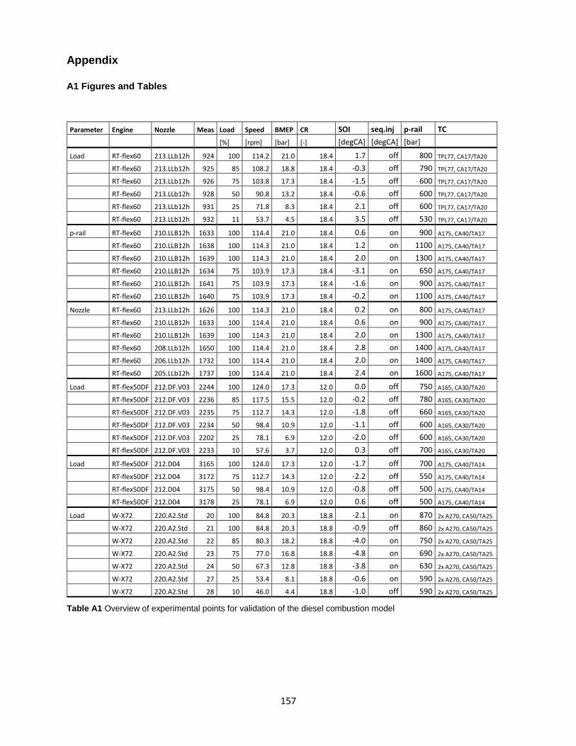
157
Appendix
A1 Figures and Tables
Parameter Engine Nozzle Meas Load Speed BMEP CR SOI seq.inj p-rail TC
[%] [rpm] [bar] [-] [degCA] [degCA] [bar]
Load RT-flex60 213.LLb12h 924 100 114.2 21.0 18.4 1.7 off 800 TPL77, CA17/TA20
RT-flex60 213.LLb12h 925 85 108.2 18.8 18.4 -0.3 off 790 TPL77, CA17/TA20
RT-flex60 213.LLb12h 926 75 103.8 17.3 18.4 -1.5 off 600 TPL77, CA17/TA20
RT-flex60 213.LLb12h 928 50 90.8 13.2 18.4 -0.6 off 600 TPL77, CA17/TA20
RT-flex60 213.LLb12h 931 25 71.8 8.3 18.4 2.1 off 600 TPL77, CA17/TA20
RT-flex60 213.LLb12h 932 11 53.7 4.5 18.4 3.5 off 530 TPL77, CA17/TA20
p-rail RT-flex60 210.LLB12h 1633 100 114.4 21.0 18.4 0.6 on 900 A175, CA40/TA17
RT-flex60 210.LLB12h 1638 100 114.3 21.0 18.4 1.2 on 1100 A175, CA40/TA17
RT-flex60 210.LLB12h 1639 100 114.3 21.0 18.4 2.0 on 1300 A175, CA40/TA17
RT-flex60 210.LLB12h 1634 75 103.9 17.3 18.4 -3.1 on 650 A175, CA40/TA17
RT-flex60 210.LLB12h 1641 75 103.9 17.3 18.4 -1.6 on 900 A175, CA40/TA17
RT-flex60 210.LLB12h 1640 75 103.9 17.3 18.4 -0.2 on 1100 A175, CA40/TA17
Nozzle RT-flex60 213.LLb12h 1626 100 114.3 21.0 18.4 0.2 on 800 A175, CA40/TA17
RT-flex60 210.LLB12h 1633 100 114.4 21.0 18.4 0.6 on 900 A175, CA40/TA17
RT-flex60 210.LLB12h 1639 100 114.3 21.0 18.4 2.0 on 1300 A175, CA40/TA17
RT-flex60 208.LLb12h 1650 100 114.4 21.0 18.4 2.8 on 1400 A175, CA40/TA17
RT-flex60 206.LLb12h 1732 100 114.4 21.0 18.4 2.0 on 1400 A175, CA40/TA17
RT-flex60 205.LLb12h 1737 100 114.4 21.0 18.4 2.4 on 1600 A175, CA40/TA17
Load RT-flex50DF 212.DF.V03 2244 100 124.0 17.3 12.0 0.0 off 750 A165, CA30/TA20
RT-flex50DF 212.DF.V03 2236 85 117.5 15.5 12.0 -0.2 off 780 A165, CA30/TA20
RT-flex50DF 212.DF.V03 2235 75 112.7 14.3 12.0 -1.8 off 660 A165, CA30/TA20
RT-flex50DF 212.DF.V03 2234 50 98.4 10.9 12.0 -1.1 off 600 A165, CA30/TA20
RT-flex50DF 212.DF.V03 2202 25 78.1 6.9 12.0 -2.0 off 600 A165, CA30/TA20
RT-flex50DF 212.DF.V03 2233 10 57.6 3.7 12.0 0.3 off 700 A165, CA30/TA20
Load RT-flex50DF 212.D04 3165 100 124.0 17.3 12.0 -1.7 off 700 A175, CA40/TA14
RT-flex50DF 212.D04 3172 75 112.7 14.3 12.0 -2.2 off 550 A175, CA40/TA14
RT-flex50DF 212.D04 3175 50 98.4 10.9 12.0 -0.8 off 500 A175, CA40/TA14
RT-flex50DF 212.D04 3178 25 78.1 6.9 12.0 0.6 off 500 A175, CA40/TA14
Load W-X72 220.A2.Std 20 100 84.8 20.3 18.8 -2.1 on 870 2x A270, CA50/TA25
W-X72 220.A2.Std 21 100 84.8 20.3 18.8 -0.9 off 860 2x A270, CA50/TA25
W-X72 220.A2.Std 22 85 80.3 18.2 18.8 -4.0 on 750 2x A270, CA50/TA25
W-X72 220.A2.Std 23 75 77.0 16.8 18.8 -4.8 on 690 2x A270, CA50/TA25
W-X72 220.A2.Std 24 50 67.3 12.8 18.8 -3.8 on 630 2x A270, CA50/TA25
W-X72 220.A2.Std 27 25 53.4 8.1 18.8 -0.6 on 590 2x A270, CA50/TA25
W-X72 220.A2.Std 28 10 46.0 4.4 18.8 -1.0 off 590 2x A270, CA50/TA25
Table A1 Overview of experimental points for validation of the diesel combustion model

158
Parameter Engine Meas Load Speed BMEP CR global Tscav PIT GAVO EVC TC
% [rpm] [bar] [-] [-] [°C] [DCATDC] [CA] [CA]
Load RT-flex50DF 3238 25 77.6 6.9 12.0 0.37 37.1 confidential ref +20.0 ref -59.0 A175, CA40/TA14
RT-flex50DF 3239 40 90.9 9.4 12.0 0.38 41.6 confidential ref +12.0 ref -44.0 A175, CA40/TA14
RT-flex50DF 3240 50 97.8 11.0 12.0 0.40 42.2 confidential ref +7.0 ref -24.0 A175, CA40/TA14
RT-flex50DF 3241 60 104.0 12.5 12.0 0.41 42.4 confidential ref +2.0 ref -16.0 A175, CA40/TA14
RT-flex50DF 3242 70 109.3 13.8 12.0 0.42 45.9 confidential ref +2.0 ref -14.0 A175, CA40/TA14
RT-flex50DF 3257 80 114.3 15.0 12.0 0.44 43.1 confidential ref +2.0 ref -9.0 A175, CA40/TA14
RT-flex50DF 3258 90 118.9 16.3 12.0 0.47 44.6 confidential ref +2.0 ref -5.0 A175, CA40/TA14
RT-flex50DF 3246 100 123.1 17.4 12.0 0.49 41.3 confidential reference reference A175, CA40/TA14
T3 RT-flex50DF 1819 85 118.1 15.6 12.0 0.39 36.8 -2.0 220 266 A165, CA30/TA20
RT-flex50DF 1820 85 118.1 15.5 12.0 0.39 41.3 -2.0 220 266 A165, CA30/TA20
RT-flex50DF 1821 85 118.1 15.5 12.0 0.39 45.9 -2.0 220 266 A165, CA30/TA20
RT-flex50DF 1822 85 118.1 15.3 12.0 0.40 52.7 -2.0 220 266 A165, CA30/TA20
RT-flex50DF 1823 85 118.0 15.6 12.0 0.40 59.2 -2.0 220 266 A165, CA30/TA20
RT-flex50DF 1824 85 118.1 15.4 12.0 0.40 62.9 -2.0 220 266 A165, CA30/TA20
RPM RT-flex50DF 1858 72 99.0 15.6 12.0 0.41 38.3 -2.0 220 266 A165, CA30/TA20
RT-flex50DF 1857 77 105.2 15.7 12.0 0.40 38.5 -2.0 220 266 A165, CA30/TA20
RT-flex50DF 1856 83 113.2 15.8 12.0 0.39 40.6 -2.0 220 266 A165, CA30/TA20
RT-flex50DF 1853 85 118.1 15.4 12.0 0.39 39.9 -2.0 220 266 A165, CA30/TA20
RT-flex50DF 1854 87 120.6 15.5 12.0 0.39 40.1 -2.0 220 266 A165, CA30/TA20
RT-flex50DF 1855 88 123.4 15.3 12.0 0.39 40.4 -2.0 220 266 A165, CA30/TA20
RT-flex50DF 1881 52 98.7 11.3 12.0 0.33 42.5 -2.0 230 266 A165, CA30/TA20
RT-flex50DF 1882 54 99.1 11.7 12.0 0.36 42.1 -2.0 230 266 A165, CA30/TA20
RT-flex50DF 1883 53 99.1 11.5 12.0 0.37 41.6 -2.0 230 266 A165, CA30/TA20
RT-flex50DF 1884 50 99.1 10.9 12.0 0.39 41.3 -2.0 230 266 A165, CA30/TA20
RT-flex50DF 1885 50 99.1 10.9 12.0 0.42 40.5 -2.0 230 266 A165, CA30/TA20
RT-flex50DF 1886 50 99.1 10.9 12.0 0.46 40.8 -2.0 230 266 A165, CA30/TA20
EVC RT-flex50DF 1880 50 98.9 10.9 12.0 0.34 40.5 0.0 230 ref -12.0 A165, CA30/TA20
RT-flex50DF 1879 50 98.9 10.9 12.0 0.35 40.8 0.0 230 ref -8.0 A165, CA30/TA20
RT-flex50DF 1874 50 99.0 10.9 12.0 0.37 40.2 0.0 230 ref -4.0 A165, CA30/TA20
RT-flex50DF 1875 50 98.9 10.9 12.0 0.39 40.7 0.0 230 reference A165, CA30/TA20
RT-flex50DF 1876 50 99.0 10.8 12.0 0.42 40.6 0.0 230 ref +4.0 A165, CA30/TA20
RT-flex50DF 1877 50 99.0 10.8 12.0 0.45 40.4 0.0 230 ref +8.0 A165, CA30/TA20
RT-flex50DF 1878 50 99.0 10.8 12.0 0.48 40.7 0.0 230 ref +12.0 A165, CA30/TA20
PIT RT-flex50DF 1897 50 99.0 11.0 12.0 0.37 41.3 2.0 230 256 A165, CA30/TA20
RT-flex50DF 1898 50 99.2 10.9 12.0 0.37 41.6 0.0 230 256 A165, CA30/TA20
RT-flex50DF 1887 50 99.1 10.9 12.0 0.37 42.1 -2.0 230 256 A165, CA30/TA20
RT-flex50DF 1899 50 99.2 10.9 12.0 0.37 41.5 -4.0 230 256 A165, CA30/TA20
RT-flex50DF 1902 49 99.1 10.8 12.0 0.37 41.2 -8.0 230 256 A165, CA30/TA20
TC match RT-flex50DF 2693 85 118.1 15.4 12.0 0.41 39.9 -2.0 reference reference A165, CA30/TA17
RT-flex50DF 2590 85 118.1 15.5 12.0 0.40 41.1 -2.0 reference reference A165, CA30/TA20
RT-flex50DF 2627 85 117.9 15.5 12.0 0.40 41.4 -2.0 reference reference A165, CA30/TA24
RT-flex50DF 2711 71 96.1 15.9 12.0 0.46 41.3 -2.0 reference reference A165, CA30/TA17
RT-flex50DF 2604 71 96.1 15.9 12.0 0.43 41.2 -2.0 reference reference A165, CA30/TA20
RT-flex50DF 2643 71 96.1 16.0 12.0 0.45 41.4 -2.0 reference reference A165, CA30/TA24
Load W-X72DF 1054 100 89.1 17.2 12.0 0.48 36.1 confidential reference reference A270, CA50/TA22
W-X72DF 1063 95 87.5 16.7 12.0 0.43 37.5 confidential ref -15.0 ref -10.0 A270, CA50/TA22
W-X72DF 1038 85 84.2 15.5 12.0 0.40 36.5 confidential ref -25.0 ref -15.0 A270, CA50/TA22
W-X72DF 1067 75 81.0 14.3 12.0 0.40 36.5 confidential ref -30.0 ref -16.0 A270, CA50/TA22
W-X72DF 1068 50 71.0 10.9 12.0 0.39 33.6 confidential ref -30.0 ref -28.0 A270, CA50/TA22
W-X72DF 1069 25 56.0 6.8 12.0 0.37 32.9 confidential ref -25.0 ref -38.0 A270, CA50/TA22
Table A2 Overview of experimental points used for validation of the DF combustion model

159
Figure A1 RT-flex50DF 1D engine model layout with integrated DF combustion model

160
A2 NO Formation
Referring to the Section 4.5.1, thermal production of nitrogen oxide according to extended Zeldovich
mechanism is conditioned by a high activation energy for breaking the nitrogen triple bound. On the other
hand, the oxidation of nitrogen atoms does not require extensive energy and hence the formation of the
nitrogen oxide corresponds to the production of nitrogen atoms. The quasi-steady assumption valid for
stoichiometric and lean conditions with sufficient oxygen availability yields equation (a1). The thermal nitric
oxide formation process can be so decoupled from the main combustion and calculated in a subsequent
time step.
𝑑[𝑁𝑂]
𝑑𝑡= 2𝑘1
+[𝑂][𝑁2]
(1 −𝑘1
−𝑘2−[𝑁𝑂]2
𝑘1+[𝑁2]𝑘2
+[𝑂2])
(1 +𝑘1
−[𝑁𝑂]𝑘2
+[𝑂2]𝑘3+[𝑂𝐻]
) (a1)
The equilibrium concentrations for oxygen and OH radicals are calculated explicitly at every time step
following the definition by equations (a2) and (a3), respectively. Concentrations are denoted by square
brackets in mole fractions and Tb is the burned zone temperature in Kelvin. Water vapor and oxygen
concentrations are determined based on in-cylinder conditions. The latter is calculated based on air
entrainment rate into the spray according to equation (x) since the mean cylinder equivalence ratio is not
representative enough for NO formation.
[𝑂] = 3.97. 105𝑇𝑏
−0.5[𝑂2]0.5𝑒
−31090𝑇𝑏 (a2)
[𝑂𝐻] = 2.129. 102𝑇𝑏
−0.57[𝑂]0.5[𝐻2𝑂]0.5𝑒−4595
𝑇𝑏 (a3)
The rate constants are numbered in ascending order for reactions (80), (81) and (82) and are based on
experimental studies. In the present study, both forward and backward reaction rate constants are
determined according to [42] and are defined by equations below.
Figure A9 illustrates instantaneous formation rates of oxygen and OH radicals in mole fraction shown on
the left y-axis of the plot. The resulting integrated NO concentration for the nominal operation of the RT-
flex60 large 2-stroke diesel engine is plotted with respect to the right y-axis. The immediate increase of
radical concentrations right after the combustion onset can be assigned to the rapid rise of the burned zone
𝑘1
+ = 1.8 × 10⁸𝑒−38370
𝑇
𝑘1− = 3.8 × 10⁷𝑒
−425𝑇
𝑘2+ = 1.8 × 10⁴𝑒
−4680𝑇
𝑘2− = 3.8 × 10³𝑒
−208020𝑇
𝑘3+ = 7.1 × 10⁷𝑒
−450𝑇
𝑘3− = 1.7 × 10⁸𝑒
−24560𝑇
(a4)
(a5)
(a6)
(a7)
(a8)
(a9)

161
temperature after ignition. In addition, the deceleration of the heat release rate due to local spray interactions
is also reflected in intermediate radical production and the final nitric oxide rate.
Figure A2 Molar fractions of O, OH and NO with respect to a select cylinder at full load operation of RT-flex60
Figure A3 compares predicted and measured NOx with assumed NO2/NOx ratio 0.2 due to the fact that no
after-oxidation of calculated nitric oxide was considered. Without any model tuning predicted NOx emissions
are generally underestimated. The largest discrepancy is related to medium and low load operation points.
Note, the presented modeling approach demonstrate an application of user defined NO formation model
but is not ready to be used for engine optimization.
Figure A3 Comparison of predicted and measured NOx formation of RT-flex60 diesel engine
A3 Heat Transfer Model
An accurate in-cylinder wall heat transfer calculation is essential for reliable engine performance predictions.
It impacts not only the overall thermal efficiency but also the effective burn rate and emission formation are
partially affected. Therefore, a suitable heat transfer modeling approach capturing both convection and
radiation is needed. For large low-speed 2-stroke diesel engines the radiation becomes of high importance
especially at lower loads where it contributes more than half of the overall heat transfer rate [14]. Such
distribution is addressed mainly to large dimensions and the nature of diffusion flame as a soot particles
source. Typically, available heat transfer models neglect the radiative heat transfer or describe it by
empirical multipliers without taking actual engine operation conditions into account. Hence, besides
describing the convective heat transfer the focus lies on defining the radiative heat transfer correspondingly
to conditions in a large 2-stroke marine engine. Besides widely used and established heat transfer concepts
[3,136] in-house NSD and ETHZ models intentionally developed and tailored for large 2-stroke marine
engines are predominantly used in an internal 0D engine cycle simulation tool DIESUL. At nominal engine
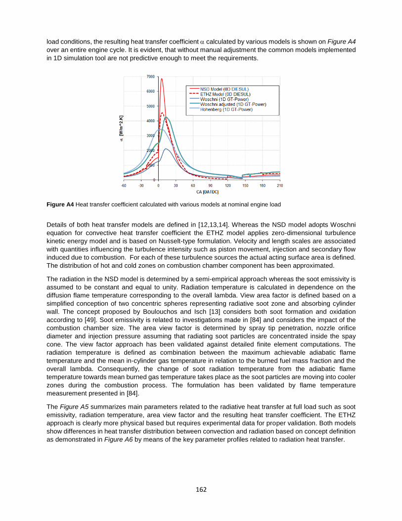
162
load conditions, the resulting heat transfer coefficient calculated by various models is shown on Figure A4
over an entire engine cycle. It is evident, that without manual adjustment the common models implemented
in 1D simulation tool are not predictive enough to meet the requirements.
Figure A4 Heat transfer coefficient calculated with various models at nominal engine load
Details of both heat transfer models are defined in [12,13,14]. Whereas the NSD model adopts Woschni
equation for convective heat transfer coefficient the ETHZ model applies zero-dimensional turbulence
kinetic energy model and is based on Nusselt-type formulation. Velocity and length scales are associated
with quantities influencing the turbulence intensity such as piston movement, injection and secondary flow
induced due to combustion. For each of these turbulence sources the actual acting surface area is defined.
The distribution of hot and cold zones on combustion chamber component has been approximated.
The radiation in the NSD model is determined by a semi-empirical approach whereas the soot emissivity is
assumed to be constant and equal to unity. Radiation temperature is calculated in dependence on the
diffusion flame temperature corresponding to the overall lambda. View area factor is defined based on a
simplified conception of two concentric spheres representing radiative soot zone and absorbing cylinder
wall. The concept proposed by Boulouchos and Isch [13] considers both soot formation and oxidation
according to [49]. Soot emissivity is related to investigations made in [84] and considers the impact of the
combustion chamber size. The area view factor is determined by spray tip penetration, nozzle orifice
diameter and injection pressure assuming that radiating soot particles are concentrated inside the spay
cone. The view factor approach has been validated against detailed finite element computations. The
radiation temperature is defined as combination between the maximum achievable adiabatic flame
temperature and the mean in-cylinder gas temperature in relation to the burned fuel mass fraction and the
overall lambda. Consequently, the change of soot radiation temperature from the adiabatic flame
temperature towards mean burned gas temperature takes place as the soot particles are moving into cooler
zones during the combustion process. The formulation has been validated by flame temperature
measurement presented in [84].
The Figure A5 summarizes main parameters related to the radiative heat transfer at full load such as soot
emissivity, radiation temperature, area view factor and the resulting heat transfer coefficient. The ETHZ
approach is clearly more physical based but requires experimental data for proper validation. Both models
show differences in heat transfer distribution between convection and radiation based on concept definition
as demonstrated in Figure A6 by means of the key parameter profiles related to radiation heat transfer.

163
Figure A5 Comparison of NSD and ETHZ heat transfer model concepts at various engine loads

164
Figure A6 Comparison of NSD and ETHZ heat transfer model concepts at various engine load
Model Formulation
The proposed heat transfer model is based on a standard Woschni approach for convection and the
radiation is based on empirical soot formation model based on work of Hiroyasu et al. [49] that was further
developed by Morel and Keribar [84] and implemented by Boulouchos et al. [13] specifically for large 2-
stroke diesel engines. The implemented model is determined mainly from literature since due to limited
availability of experimental data only a small part of the model could be validated. Essentially, the total wall
heat transfer is a sum of the convective and radiative losses. Assuming the heat transfer to be quasi-steady
process the convective instantaneous specific heat transfer rate �̇�𝑐𝑜𝑛𝑣 can be formulated by equation (a10)
following the approach of Woschni [136]. The heat transfer coefficient is related to the cylinder bore B, in-
cylinder pressure and gas temperature T and the characteristic velocity term defined in the brackets that
depends on the mean piston speed um, displacement volume Vdispl, reference state conditions and the
difference between actual and motored pressure p0. Coefficients C1 and C2 consider the gas velocity
changes during the engine cycle.
�̇�𝑐𝑜𝑛𝑣 = 𝐶𝑐𝑜𝑛𝑣 𝐵−0.2 𝑝0.8 𝑇−0.53 (𝐶1𝑢𝑚 + 𝐶2
𝑉𝑑𝑖𝑠𝑝𝑙𝑇𝑟𝑒𝑓
𝑝𝑟𝑒𝑓𝑉𝑟𝑒𝑓
(𝑝 − 𝑝0))
0.8
(𝑇 − 𝑇𝑤) (a10)
The radiative heat flux is based on the Stefan-Boltzmann law describing the radiation power of a black body
from its temperature. The radiative heat flux can be correlated by a relation as proposed by Annand [3] and
further developed by various authors defining key factors such as radiation soot temperature, radiation
emissivity and absorption and the viewing factor taking the geometry and spatial distribution of the radiative
heat flux into account. The instantaneous radiation heat flux is defined by equation (a11) where 𝑠, 𝑤 are

165
soot and wall emissivity respectively, Stefan-Bolzmann constant and 𝑠,𝑤
is the area view factor for soot
radiation into walls.
�̇�𝑟𝑎𝑑 = 𝑠 𝑤 𝑠,𝑤
(𝑇𝑟𝑎𝑑4 − 𝑇𝑤
4) (a11)
All individual parameters need to be resolved with respect to instantaneous in-cylinder conditions and
related to the combustion chamber area to gain the final radiation heat loss. The wall emissivity and thus
also absorption is assumed to equal unity and hence completely absorb all incident rays arising from soot
radiation as an idealized black body. To determine the soot emissivity, several simplifying assumptions are
prerequisite including uniform soot distribution within the burned zone, constant temperature and no
dependency on the emittance wavelength. Then, the soot emissivity is calculated by (a12) where the fv is
the volume fraction occupied by soot and fv the characteristic zone thickness.
𝑠 = 1 − 𝑒𝑥𝑝 (−1575 𝑓𝑣 𝑙𝑠 𝑇𝑟𝑎𝑑) (a12)
Soot formation and oxidation model is needed to define the actual mass of soot that is used to calculate the soot volume fraction fv.
𝑓𝑣 =
𝑚𝑠
𝜌𝑠
1
𝑉𝑐𝑦𝑙
(a13)
Analogous to the concept proposed in [13] the characteristic zone thickness is specified as a surface area to volume ratio as defined below.
𝑓𝑠 = 𝐵 (
3
16
𝑠𝑡𝑟𝑜𝑘𝑒/𝐵
𝑉𝑑𝑖𝑠𝑝𝑙/𝑉𝑐𝑦𝑙
)
1/3
(a14)
Following the approach introduced in [49] and later applied for heat transfer modeling for DI diesel engine
[12] soot formation rate is calculated by assuming a first-order reaction of vaporized fuel. The formation is
closely linked to the combustion process and is characterized by dependence on temperature and
equivalence ratio expressed in the form of molar oxygen concentration YO2.
𝑑𝑚𝑠,𝑓𝑜
𝑑𝑡= 0.38
𝑚𝑓,𝑏
𝑑𝑡 𝑒𝑥𝑝 (
−5000
𝑇𝑟𝑎𝑑
) 1
1 + 𝑌𝑂2
(a15)
The subsequent soot oxidation is predicted by assuming a second order reaction considering the actual
soot mass, soot density, diameter of elementary soot particle (0.04m) and the partial oxygen pressure in
the burned zone.
𝑑𝑚𝑠,𝑜𝑥
𝑑𝑡= −0.015
𝑚𝑠
𝜌𝑠𝑑𝑠
𝑒𝑥𝑝 (5000
𝑇𝑟𝑎𝑑
) 𝑝𝑂20.5 (a16)
The crank angle based soot formation and oxidation rates are plotted in Figure A6 for the nominal engine
load conditions. As shown, the soot formation duplicates the progress of burn rate whereas the oxidation is
delayed and takes place predominantly in the later combustion phase. However, after the combustion is
terminated merely a partial oxidation is possible due to low temperature level.

166
Figure A6 Soot formation and oxidation rate at nominal engine load
Available experimental data from the RT-flex60 (RTX-4) test engine for LFO operation considering various
tuning versions, injector nozzles and introducing of cooled EGR are compared with the empirical soot model
over the engine load in Figure A7. Considering the fact, that the soot formation and oxidation are complex
phenomena affected by multiple factors such as local conditions and concentrations, injections strategies
or fuel properties, the suggested model is capable to capture trends only. Nevertheless, for the intended
application and due to the scope of present work the results are acceptable.
Figure A7 Comparison of the empirical soot model with RT-flex60 experimental results
In general, the area view factor s,w is used to parameterize the fraction of thermal energy being emitted by
glowing particulates and reaching combustion space walls. Based on its definition it is a dimensionless
parameter and can reach a maximum value of unity for a limit case when all the emitted radiation can be
impinged on the walls surface. The simple approach linked to the heat release profile incorporated in the
NSD model overestimates the radiative heat transfer. The concept utilized in the present model and
proposed in [13] adopts a correlation linked to the ratio of the penetrated spray area Aspray to the overall
piston area Apiston in a form of an exponential function as defined by equations (a17) and (a18).

167
𝑠,𝑤= 𝐶1 (1 − exp (−𝐶2
𝐴𝑠𝑝𝑟𝑎𝑦
𝐴𝑝𝑖𝑠𝑡𝑜𝑛
)) (a17)
𝐴𝑠𝑝𝑟𝑎𝑦
𝐴𝑝𝑖𝑠𝑡𝑜𝑛
= 8 tan (𝜃
2) (
√13.8 𝑢𝑖𝑛𝑗 𝑑𝑛𝑜𝑧 𝑡
𝐵) (a18)
Due to the dependency of the radiative heat flux on the fourth power of the radiation temperature, the correct
determination of the radiation temperature is substantial. However, the prediction is linked to difficulties to
experimental measurement and validation. Various approaches can be found in literature mainly linked
directly to the burned zone temperature. Boulouchos and Isch [13] proposed a defined by weighting factors
to be between the maximum adiabatic and mean process temperatures. The link to equivalence ratio
represent the fact that the radiation of oxidized soot particles is significantly higher that the remaining soot
amount formed in the early combustion phase. In the present model the radiation temperature is calculated
based on the approach of Morel and Keribar [86] as defined in equation (a19). The concept accounts for
heat transfer from the soot particle itself by reducing the burned zone temperature Tb to determine the
radiation temperature. Since the soot formation takes place within rich flame zones and with the combustion
progress the radiation temperature drop significantly the radiation temperature is related to the ratio of
unburned mass to the total in-cylinder mass.
𝑇𝑟𝑎𝑑 = 0.9 (
𝑚𝑐𝑦𝑙,𝑏
𝑚𝑐𝑦𝑙,𝑡𝑜𝑡
𝑇𝑏 + (1 −𝑚𝑐𝑦𝑙,𝑏
𝑚𝑐𝑦𝑙,𝑡𝑜𝑡
)𝑇𝑏,𝑚𝑎𝑥) (a19)
Figure A8 Radiation heat transfer model results implemented in 1D cycle simulation for soot emissivity s, soot volume
fraction fv, radiation temperature Trad and area view factor s,w over the engine load variation

168
The heat transfer model is implemented into a cycle simulation tool by means of a user subroutine.
Practically, no additional computational time is required due to user heat transfer model thanks to a relative
simple code structure. Major parameters related to the radiation heat transfer model such as soot emissivity,
soot volume fraction, radiation temperature and the area view factor are plotted in Figure A8. Crank based
profiles of each parameter are shown for load sweep on a theoretical propeller curve using a 1D RT-flex60
test engine model.
The resulting radiation and convection heat fluxes for the identical engine load variation are plotted on the
Figure A9. Quantitatively, it is worth mentioning that the soot radiation is relevant mainly for the short period
of time as the combustion occurs. Moreover, it can be observed that at high load operation the convective
heat transfer is predominant but the radiation becomes more pronounced as the load decreases. In
conclusion, a physical based radiation modeling enables creating a predictive model for a specific condition
in a large 2-stroke engine. The proposed model can be directly used in a commercial 1D engine cycle
simulation tool. Additional validation process against experimental data especially in terms of radiation
temperature and soot formation can further improve the model fidelity.
Figure A9 Radiative and convective heat flux calculated with present model