Czech Technical University in Prague, Faculty of Civil Engineering

&

Université Grenoble I – Joseph Fourier, École doctorale I-MEP2

PhD thesisin computational mechanics

presented by

Václav Šmilauer

defended June 24th 2010

Cohesive Particle Modelusing the Discrete Element Method

on the Yade Platform

defense committeeZdeněk Bittnar professor, CTU Prague presidentJan Vítek professor, Metrostav reviewerAli Limam professor, INSA Lyon reviewerBořek Patzák assoc. professor, CTU Prague examinatorBruno Chareyre assoc. professor, UJF Grenoble examinator

PhD, industry examinatorPhD, industry guest

Milan Jirásek professor, CTU Prague supervisorLaurent Daudeville professor, UJF Grenoble supervisor

ČESKÉ VYSOKÉ UČENÍ TECHNICKÉ V PRAZEFakulta stavební

ve spolupráci s Université Grenoble I – Joseph Fourier

Doktorský studijní program: Stavební inženýrstvíStudijní obor: Fyzikální a materiálové inženýrství

Mgr. Ing. Václav Šmilauer

Cohesive Particle Model using the Discrete Element Method on the Yade PlatformModel kohezivních částic pomocí metody diskrétních prvků na platformě Yade

Disertační práce k získání akademického titulu Ph.D.

Školitelé: Prof. Ing. Milan Jirásek, DrSc.Prof. Laurent Daudeville

Praha, Červen 2010

Acknowledgements

I am deeply indebted to numerous people at organizational, professional, inter-personal and intra-personallevels. Although they are too many to be mentioned here one by one, the concern of omitting someonedoes not present good reason to not mention anyone at all. Suffices to say that omissions are notdisacknowledgements and that order of text should not suggest importance.

With the hope of giving back, directly or indirectly, all I received, I would like to express, therefore, mysincere thanks to (in no particular order)

• thesis supervisors Milan Jirásek at Czech Technical University in Prague, for his patience andpersonal and collegial attitude; Laurent Daudeville at Université Joseph Fourier in Grenoble, forhis greatly appreciated support during difficult beginnings of the PhD,

• Ministère de l’enseignement supérieur et de la recherche, Grantová Agentura České republiky andthe industrial partner for funding;

• my colleagues Anton Gladky, Sergei Dorofeenko, Bruno Chareyre, Jan Kozicki, Fréderic VictorDonzé, Chiara Modenese, David Mašín, Claudio Tamagnini, Michal Kotrč, Vít Šmilauer, RůženaChamrová, Denis Davydov for questions, discussions and challenges;

• my parents;

• administrative support of Linda Fournier, Anne-Cécile Combe, Carole Didonato, Věra Pokorná,Alexandra Kurfürstová, Daniela Ambrožová, Veronika Kabilková, for giving human face to inhumanpaperwork;

• my students, for their questions and criticism, and for the honor of becoming friend of several ofthem;

• authors of great open-source codes, especially: TEX and friends (XƎLATEX), Python, GNU Com-piler Collection, Boost libraries, Matplotlib, Linux kernel, Ubuntu, Debian, Vim, IPE, Bazaar,Launchpad.net;

• Lukáš Bernard and Rémi Cailletaud for professional and supportive IT backing;

• my friends Ludmila Divišová, Eva Romancovová, Helena Schalková, Berenika Kučerová, MikulášKosák, Jan Kopecký, Jan Pospíšil, Marie Kindermannová, Klára Mesanyová, Jitka Špičková, HanaŠantrůčková, Meri Lampinen, Petr Máj, Stéphanie Vignand, Benedikt Vangeli, Jana Havlová,Jiří Holba, Daniel Suk, Justina Trlifajová, Michal Hrouzek, Michal Knotek, Martin Ježek, MarieKriegelová, Kateřina Pekárková, Helena Svobodová for their support, tolerance, inspiration andeverything else;

• my music soulmates Václav Hausenblas, David Čížek, Marek Novotný, Zbyněk Polívka, Jakub Klár,Denisa Martínková, Tereza Rejšková, Magdalena Klárová, Laurent Coq, Beata Hlavenková, OndřejPivec, Joel Frahm, Brad Mehldau, Michael Wollny, Kurt Rosenwinkel, Wayne Shorter, JoshuaRedman, Sidonius Karez, Johann Sebastian Bach, John Eliot Gardiner for inspiration which wouldbe infinite if my mind were infinitely open;

• Mariana Cecilie Svobodová for true bōdhisattva compassion;

• my teachers of openness Miloš Hrdý, Milada Hrdá, Tomáš Vystrčil, Ivan Špička, Mary Irene Bock-over, Carl Gustav Jung, Marie-Louise von Franz, Rob Preece, Vladimír Holan, Robert Musil, VáclavČerný, Irvin D. Yalom and others;

• Μουσική & शनयता.

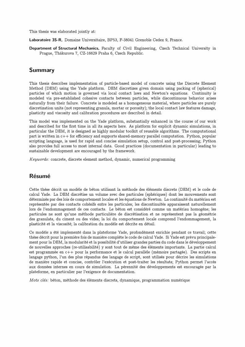
This thesis was elaborated jointly at:

Laboratoire 3S-R, Domaine Universitaire, BP53, F-38041 Grenoble Cedex 9, France.

Department of Structural Mechanics, Faculty of Civil Engineering, Czech Technical University inPrague, Thákurova 7, CZ-16629 Praha 6, Czech Republic.

Summary

This thesis describes implementation of particle-based model of concrete using the Discrete ElementMethod (DEM) using the Yade platform. DEM discretizes given domain using packing of (spherical)particles of which motion is governed via local contact laws and Newton’s equations. Continuity ismodeled via pre-established cohesive contacts between particles, while discontinuous behavior arisesnaturally from their failure. Concrete is modeled as a homogeneous material, where particles are purelydiscretization units (not representing granula, mortar or porosity); the local contact law features damage,plasticity and viscosity and calibration procedures are described in detail.

This model was implemented on the Yade platform, substantially enhanced in the course of our workand described for the first time in all its aspects here. As platform for explicit dynamic simulations, inparticular the DEM, it is designed as highly modular toolkit of reusable algorithms. The computationalpart is written in c++ for efficiency and supports shared-memory parallel computation. Python, popularscripting language, is used for rapid and concise simulation setup, control and post-processing; Pythonalso provides full access to most internal data. Good practices (documentation in particular) leading tosustainable development are encouraged by the framework.

Keywords: concrete, discrete element method, dynamic, numerical programming

Résumé

Cette thèse décrit un modèle de béton utilisant la méthode des éléments discrets (DEM) et le code decalcul Yade. La DEM discrétise un volume avec des particules (sphériques) dont les mouvements sontdéterminés par des lois de comportement locales et les équations de Newton. La continuité du matériau estreprésentée par des contacts cohésifs entre les particules; les discontinuités apparaissent naturellementlors de l’endommagement de ces contacts. Le béton est considéré comme un matériau homogène; lesparticules ne sont qu’une méthode particulière de discrétisation et ne représentent pas la géométriedes granulats, du ciment ou des vides; la loi du comportement locale comprend l’endommagement, laplasticité et la viscosité; la calibration du modèle est décrite en détail.

Ce modèle a été implementé dans la plateforme Yade, profondément enrichie pendant ce travail; cettethèse décrit pour la première fois de manière complète le code de calcul Yade. Si Yade est prévu principale-ment pour la DEM, la modularité et la possibilité d’utiliser grandes parties du code dans le développementde nouvelles approches (re-utilisabilité) y sont tout de même des éléments importants. La partie calculest programmée en c++ pour la performance et le calcul parallèle (mémoire partagée). Des scripts enlangage python, l’un des plus répandus des langage de script, sont utilisés pour décrire les simulationsde manière rapide et concise, contrôler l’exécution et post-traiter les résultats; Python permet l’accèsaux données internes en cours de simulation. La pérennité des développements est encouragée par laplateforme, en particulier par l’exigence de documentation.

Mots clés: béton, méthode des éléments discrets, dynamique, programmation numérique

Contents

Notation . . . . . . . . . . . . . . . . . . . . . . . . . . . . . . . . . . . . . . . . . . . . . . . . . 1

Introduction 3

I. Concrete particle model 5

1. Discrete Element Method 71.1. Characterisation . . . . . . . . . . . . . . . . . . . . . . . . . . . . . . . . . . . . . . . . . 71.2. Feature variations . . . . . . . . . . . . . . . . . . . . . . . . . . . . . . . . . . . . . . . . 8

1.2.1. Space dimension . . . . . . . . . . . . . . . . . . . . . . . . . . . . . . . . . . . . . 81.2.2. Particle geometry . . . . . . . . . . . . . . . . . . . . . . . . . . . . . . . . . . . . . 81.2.3. Contact detection algorithm . . . . . . . . . . . . . . . . . . . . . . . . . . . . . . . 81.2.4. Boundary conditions . . . . . . . . . . . . . . . . . . . . . . . . . . . . . . . . . . . 91.2.5. Particle deformability . . . . . . . . . . . . . . . . . . . . . . . . . . . . . . . . . . 91.2.6. Cohesion and fracturing . . . . . . . . . . . . . . . . . . . . . . . . . . . . . . . . . 91.2.7. Time integration scheme . . . . . . . . . . . . . . . . . . . . . . . . . . . . . . . . . 10

1.3. Micro-macro behavior relations . . . . . . . . . . . . . . . . . . . . . . . . . . . . . . . . . 10

2. Problem formulation 112.1. Collision detection . . . . . . . . . . . . . . . . . . . . . . . . . . . . . . . . . . . . . . . . 11

2.1.1. Generalities . . . . . . . . . . . . . . . . . . . . . . . . . . . . . . . . . . . . . . . . 112.1.2. Algorithms . . . . . . . . . . . . . . . . . . . . . . . . . . . . . . . . . . . . . . . . 122.1.3. Sweep and prune . . . . . . . . . . . . . . . . . . . . . . . . . . . . . . . . . . . . . 12

2.2. Creating interaction between particles . . . . . . . . . . . . . . . . . . . . . . . . . . . . . 152.2.1. Stiffnesses . . . . . . . . . . . . . . . . . . . . . . . . . . . . . . . . . . . . . . . . . 152.2.2. Other parameters . . . . . . . . . . . . . . . . . . . . . . . . . . . . . . . . . . . . . 16

2.3. Strain evaluation . . . . . . . . . . . . . . . . . . . . . . . . . . . . . . . . . . . . . . . . . 172.3.1. Normal strain . . . . . . . . . . . . . . . . . . . . . . . . . . . . . . . . . . . . . . . 172.3.2. Shear strain . . . . . . . . . . . . . . . . . . . . . . . . . . . . . . . . . . . . . . . . 19

2.4. Stress evaluation (example) . . . . . . . . . . . . . . . . . . . . . . . . . . . . . . . . . . . 212.5. Motion integration . . . . . . . . . . . . . . . . . . . . . . . . . . . . . . . . . . . . . . . . 22

2.5.1. Position . . . . . . . . . . . . . . . . . . . . . . . . . . . . . . . . . . . . . . . . . . 232.5.2. Orientation (spherical) . . . . . . . . . . . . . . . . . . . . . . . . . . . . . . . . . . 232.5.3. Orientation (aspherical) . . . . . . . . . . . . . . . . . . . . . . . . . . . . . . . . . 242.5.4. Clumps (rigid aggregates) . . . . . . . . . . . . . . . . . . . . . . . . . . . . . . . . 252.5.5. Numerical damping . . . . . . . . . . . . . . . . . . . . . . . . . . . . . . . . . . . 252.5.6. Stability considerations . . . . . . . . . . . . . . . . . . . . . . . . . . . . . . . . . 26

2.6. Periodic boundary conditions . . . . . . . . . . . . . . . . . . . . . . . . . . . . . . . . . . 292.6.1. Collision detection in periodic cell . . . . . . . . . . . . . . . . . . . . . . . . . . . 30

2.7. Computational aspects . . . . . . . . . . . . . . . . . . . . . . . . . . . . . . . . . . . . . . 332.7.1. Cost . . . . . . . . . . . . . . . . . . . . . . . . . . . . . . . . . . . . . . . . . . . . 332.7.2. Result indeterminism . . . . . . . . . . . . . . . . . . . . . . . . . . . . . . . . . . 34

3. Concrete particle model 373.1. Discrete concrete models overview . . . . . . . . . . . . . . . . . . . . . . . . . . . . . . . 373.2. Model description . . . . . . . . . . . . . . . . . . . . . . . . . . . . . . . . . . . . . . . . . 38

3.2.1. Cohesive and non-cohesive contacts . . . . . . . . . . . . . . . . . . . . . . . . . . 383.2.2. Contact parameters . . . . . . . . . . . . . . . . . . . . . . . . . . . . . . . . . . . 383.2.3. Normal stresses . . . . . . . . . . . . . . . . . . . . . . . . . . . . . . . . . . . . . . 38

v

3.2.4. Shear stresses . . . . . . . . . . . . . . . . . . . . . . . . . . . . . . . . . . . . . . . 443.2.5. Applying stresses on particles . . . . . . . . . . . . . . . . . . . . . . . . . . . . . . 463.2.6. Contact model summary . . . . . . . . . . . . . . . . . . . . . . . . . . . . . . . . . 46

3.3. Parameter calibration . . . . . . . . . . . . . . . . . . . . . . . . . . . . . . . . . . . . . . 473.3.1. Simulation setup . . . . . . . . . . . . . . . . . . . . . . . . . . . . . . . . . . . . . 483.3.2. Geometry and elastic parameters . . . . . . . . . . . . . . . . . . . . . . . . . . . . 503.3.3. Damage and plasticity parameters . . . . . . . . . . . . . . . . . . . . . . . . . . . 533.3.4. Confinement parameters . . . . . . . . . . . . . . . . . . . . . . . . . . . . . . . . . 543.3.5. Rate-dependence parameters . . . . . . . . . . . . . . . . . . . . . . . . . . . . . . 56

II. The Yade platform 61

4. Overview 634.1. History . . . . . . . . . . . . . . . . . . . . . . . . . . . . . . . . . . . . . . . . . . . . . . 634.2. Software architecture . . . . . . . . . . . . . . . . . . . . . . . . . . . . . . . . . . . . . . . 63

4.2.1. Documentation . . . . . . . . . . . . . . . . . . . . . . . . . . . . . . . . . . . . . . 644.2.2. Modularity . . . . . . . . . . . . . . . . . . . . . . . . . . . . . . . . . . . . . . . . 644.2.3. Serialization . . . . . . . . . . . . . . . . . . . . . . . . . . . . . . . . . . . . . . . . 654.2.4. Python interface . . . . . . . . . . . . . . . . . . . . . . . . . . . . . . . . . . . . . 654.2.5. Parallel computation . . . . . . . . . . . . . . . . . . . . . . . . . . . . . . . . . . . 664.2.6. Dispatchers and functors . . . . . . . . . . . . . . . . . . . . . . . . . . . . . . . . 67

5. Introduction 695.1. Getting started . . . . . . . . . . . . . . . . . . . . . . . . . . . . . . . . . . . . . . . . . . 69

5.1.1. Starting yade . . . . . . . . . . . . . . . . . . . . . . . . . . . . . . . . . . . . . . . 695.1.2. Creating simulation . . . . . . . . . . . . . . . . . . . . . . . . . . . . . . . . . . . 705.1.3. Running simulation . . . . . . . . . . . . . . . . . . . . . . . . . . . . . . . . . . . 705.1.4. Saving and loading . . . . . . . . . . . . . . . . . . . . . . . . . . . . . . . . . . . . 715.1.5. Graphical interface . . . . . . . . . . . . . . . . . . . . . . . . . . . . . . . . . . . . 72

5.2. Architecture overview . . . . . . . . . . . . . . . . . . . . . . . . . . . . . . . . . . . . . . 735.2.1. Data and functions . . . . . . . . . . . . . . . . . . . . . . . . . . . . . . . . . . . . 73

6. User’s manual 796.1. Scene construction . . . . . . . . . . . . . . . . . . . . . . . . . . . . . . . . . . . . . . . . 79

6.1.1. Triangulated surfaces . . . . . . . . . . . . . . . . . . . . . . . . . . . . . . . . . . 796.1.2. Sphere packings . . . . . . . . . . . . . . . . . . . . . . . . . . . . . . . . . . . . . 806.1.3. Adding particles . . . . . . . . . . . . . . . . . . . . . . . . . . . . . . . . . . . . . 856.1.4. Creating interactions . . . . . . . . . . . . . . . . . . . . . . . . . . . . . . . . . . . 876.1.5. Base engines . . . . . . . . . . . . . . . . . . . . . . . . . . . . . . . . . . . . . . . 896.1.6. Imposing conditions . . . . . . . . . . . . . . . . . . . . . . . . . . . . . . . . . . . 926.1.7. Convenience features . . . . . . . . . . . . . . . . . . . . . . . . . . . . . . . . . . . 93

6.2. Controlling simulation . . . . . . . . . . . . . . . . . . . . . . . . . . . . . . . . . . . . . . 956.2.1. Tracking variables . . . . . . . . . . . . . . . . . . . . . . . . . . . . . . . . . . . . 956.2.2. Stop conditions . . . . . . . . . . . . . . . . . . . . . . . . . . . . . . . . . . . . . . 986.2.3. Remote control . . . . . . . . . . . . . . . . . . . . . . . . . . . . . . . . . . . . . . 1006.2.4. Batch queuing and execution (yade-multi) . . . . . . . . . . . . . . . . . . . . . . . 101

6.3. Postprocessing . . . . . . . . . . . . . . . . . . . . . . . . . . . . . . . . . . . . . . . . . . 1076.4. Extending Yade . . . . . . . . . . . . . . . . . . . . . . . . . . . . . . . . . . . . . . . . . . 1076.5. Troubleshooting . . . . . . . . . . . . . . . . . . . . . . . . . . . . . . . . . . . . . . . . . 107

6.5.1. Crashes . . . . . . . . . . . . . . . . . . . . . . . . . . . . . . . . . . . . . . . . . . 1076.5.2. Reporting bugs . . . . . . . . . . . . . . . . . . . . . . . . . . . . . . . . . . . . . . 1086.5.3. Getting help . . . . . . . . . . . . . . . . . . . . . . . . . . . . . . . . . . . . . . . 108

7. Programmer’s manual 1117.1. Build system . . . . . . . . . . . . . . . . . . . . . . . . . . . . . . . . . . . . . . . . . . . 111

7.1.1. Pre-build configuration . . . . . . . . . . . . . . . . . . . . . . . . . . . . . . . . . 1117.1.2. Building . . . . . . . . . . . . . . . . . . . . . . . . . . . . . . . . . . . . . . . . . . 113

vi

7.2. Conventions . . . . . . . . . . . . . . . . . . . . . . . . . . . . . . . . . . . . . . . . . . . . 1157.2.1. Class naming . . . . . . . . . . . . . . . . . . . . . . . . . . . . . . . . . . . . . . . 1167.2.2. Documentation . . . . . . . . . . . . . . . . . . . . . . . . . . . . . . . . . . . . . . 117

7.3. Support framework . . . . . . . . . . . . . . . . . . . . . . . . . . . . . . . . . . . . . . . . 1197.3.1. Pointers . . . . . . . . . . . . . . . . . . . . . . . . . . . . . . . . . . . . . . . . . . 1197.3.2. Basic numerics . . . . . . . . . . . . . . . . . . . . . . . . . . . . . . . . . . . . . . 1207.3.3. Run-time type identification (RTTI) . . . . . . . . . . . . . . . . . . . . . . . . . . 1217.3.4. Serialization . . . . . . . . . . . . . . . . . . . . . . . . . . . . . . . . . . . . . . . . 1217.3.5. YADE_CLASS_BASE_DOC_* macro family . . . . . . . . . . . . . . . . . . . . 1257.3.6. Multiple dispatch . . . . . . . . . . . . . . . . . . . . . . . . . . . . . . . . . . . . . 1287.3.7. Parallel execution . . . . . . . . . . . . . . . . . . . . . . . . . . . . . . . . . . . . 1337.3.8. Logging . . . . . . . . . . . . . . . . . . . . . . . . . . . . . . . . . . . . . . . . . . 1347.3.9. Timing . . . . . . . . . . . . . . . . . . . . . . . . . . . . . . . . . . . . . . . . . . 1357.3.10. OpenGL Rendering . . . . . . . . . . . . . . . . . . . . . . . . . . . . . . . . . . . 137

7.4. Simulation framework . . . . . . . . . . . . . . . . . . . . . . . . . . . . . . . . . . . . . . 1387.4.1. Scene . . . . . . . . . . . . . . . . . . . . . . . . . . . . . . . . . . . . . . . . . . . 1387.4.2. Body container . . . . . . . . . . . . . . . . . . . . . . . . . . . . . . . . . . . . . . 1387.4.3. InteractionContainer . . . . . . . . . . . . . . . . . . . . . . . . . . . . . . . . . . . 1397.4.4. ForceContainer . . . . . . . . . . . . . . . . . . . . . . . . . . . . . . . . . . . . . . 1407.4.5. Handling interactions . . . . . . . . . . . . . . . . . . . . . . . . . . . . . . . . . . 141

7.5. Runtime structure . . . . . . . . . . . . . . . . . . . . . . . . . . . . . . . . . . . . . . . . 1427.5.1. Startup sequence . . . . . . . . . . . . . . . . . . . . . . . . . . . . . . . . . . . . . 1437.5.2. Singletons . . . . . . . . . . . . . . . . . . . . . . . . . . . . . . . . . . . . . . . . . 1437.5.3. Engine loop . . . . . . . . . . . . . . . . . . . . . . . . . . . . . . . . . . . . . . . . 144

7.6. Python framework . . . . . . . . . . . . . . . . . . . . . . . . . . . . . . . . . . . . . . . . 1447.6.1. Wrapping c++ classes . . . . . . . . . . . . . . . . . . . . . . . . . . . . . . . . . . 1447.6.2. Subclassing c++ types in python . . . . . . . . . . . . . . . . . . . . . . . . . . . . 1457.6.3. Reference counting . . . . . . . . . . . . . . . . . . . . . . . . . . . . . . . . . . . . 1457.6.4. Custom converters . . . . . . . . . . . . . . . . . . . . . . . . . . . . . . . . . . . . 145

7.7. Maintaining compatibility . . . . . . . . . . . . . . . . . . . . . . . . . . . . . . . . . . . . 1467.7.1. Renaming class . . . . . . . . . . . . . . . . . . . . . . . . . . . . . . . . . . . . . . 1467.7.2. Renaming class attribute . . . . . . . . . . . . . . . . . . . . . . . . . . . . . . . . 147

7.8. Debian packaging instructions . . . . . . . . . . . . . . . . . . . . . . . . . . . . . . . . . . 1477.8.1. Prepare source package . . . . . . . . . . . . . . . . . . . . . . . . . . . . . . . . . 1477.8.2. Create binary package . . . . . . . . . . . . . . . . . . . . . . . . . . . . . . . . . . 148

8. Conclusion 149

III. Appendices 151

A. Object-oriented programming paradigm 153A.1. Key concepts . . . . . . . . . . . . . . . . . . . . . . . . . . . . . . . . . . . . . . . . . . . 153A.2. Language support and performance . . . . . . . . . . . . . . . . . . . . . . . . . . . . . . . 154

B. Quaternions 157B.1. Unit quaternions as spatial rotations . . . . . . . . . . . . . . . . . . . . . . . . . . . . . . 158B.2. Comparison of spatial rotation representations . . . . . . . . . . . . . . . . . . . . . . . . 159

C. Class reference (yade.wrapper module) 161C.1. Bodies . . . . . . . . . . . . . . . . . . . . . . . . . . . . . . . . . . . . . . . . . . . . . . . 161

C.1.1. Body . . . . . . . . . . . . . . . . . . . . . . . . . . . . . . . . . . . . . . . . . . . . 161C.1.2. Shape . . . . . . . . . . . . . . . . . . . . . . . . . . . . . . . . . . . . . . . . . . . 162C.1.3. State . . . . . . . . . . . . . . . . . . . . . . . . . . . . . . . . . . . . . . . . . . . . 163C.1.4. Material . . . . . . . . . . . . . . . . . . . . . . . . . . . . . . . . . . . . . . . . . . 164C.1.5. Bound . . . . . . . . . . . . . . . . . . . . . . . . . . . . . . . . . . . . . . . . . . . 166

C.2. Interactions . . . . . . . . . . . . . . . . . . . . . . . . . . . . . . . . . . . . . . . . . . . . 166C.2.1. Interaction . . . . . . . . . . . . . . . . . . . . . . . . . . . . . . . . . . . . . . . . 166C.2.2. InteractionGeometry . . . . . . . . . . . . . . . . . . . . . . . . . . . . . . . . . . . 167

vii

C.2.3. InteractionPhysics . . . . . . . . . . . . . . . . . . . . . . . . . . . . . . . . . . . . 169C.3. Global engines . . . . . . . . . . . . . . . . . . . . . . . . . . . . . . . . . . . . . . . . . . 175C.4. Partial engines . . . . . . . . . . . . . . . . . . . . . . . . . . . . . . . . . . . . . . . . . . 193C.5. Bounding volume creation . . . . . . . . . . . . . . . . . . . . . . . . . . . . . . . . . . . . 195

C.5.1. BoundFunctor . . . . . . . . . . . . . . . . . . . . . . . . . . . . . . . . . . . . . . 195C.5.2. BoundDispatcher . . . . . . . . . . . . . . . . . . . . . . . . . . . . . . . . . . . . . 196

C.6. Interaction Geometry creation . . . . . . . . . . . . . . . . . . . . . . . . . . . . . . . . . . 196C.6.1. InteractionGeometryFunctor . . . . . . . . . . . . . . . . . . . . . . . . . . . . . . 196C.6.2. InteractionGeometryDispatcher . . . . . . . . . . . . . . . . . . . . . . . . . . . . . 197

C.7. Interaction Physics creation . . . . . . . . . . . . . . . . . . . . . . . . . . . . . . . . . . . 198C.7.1. InteractionPhysicsFunctor . . . . . . . . . . . . . . . . . . . . . . . . . . . . . . . . 198C.7.2. InteractionPhysicsDispatcher . . . . . . . . . . . . . . . . . . . . . . . . . . . . . . 200

C.8. Constitutive laws . . . . . . . . . . . . . . . . . . . . . . . . . . . . . . . . . . . . . . . . . 201C.8.1. LawFunctor . . . . . . . . . . . . . . . . . . . . . . . . . . . . . . . . . . . . . . . . 201C.8.2. LawDispatcher . . . . . . . . . . . . . . . . . . . . . . . . . . . . . . . . . . . . . . 203

C.9. Callbacks . . . . . . . . . . . . . . . . . . . . . . . . . . . . . . . . . . . . . . . . . . . . . 204C.9.1. BodyCallback . . . . . . . . . . . . . . . . . . . . . . . . . . . . . . . . . . . . . . . 204C.9.2. IntrCallback . . . . . . . . . . . . . . . . . . . . . . . . . . . . . . . . . . . . . . . . 204

C.10.Preprocessors . . . . . . . . . . . . . . . . . . . . . . . . . . . . . . . . . . . . . . . . . . . 204C.11.Rendering . . . . . . . . . . . . . . . . . . . . . . . . . . . . . . . . . . . . . . . . . . . . . 208

C.11.1.OpenGLRenderingEngine . . . . . . . . . . . . . . . . . . . . . . . . . . . . . . . . 208C.11.2.GlShapeFunctor . . . . . . . . . . . . . . . . . . . . . . . . . . . . . . . . . . . . . 209C.11.3.GlStateFunctor . . . . . . . . . . . . . . . . . . . . . . . . . . . . . . . . . . . . . . 210C.11.4.GlBoundFunctor . . . . . . . . . . . . . . . . . . . . . . . . . . . . . . . . . . . . . 210C.11.5.GlInteractionGeometryFunctor . . . . . . . . . . . . . . . . . . . . . . . . . . . . . 210C.11.6.GlInteractionPhysicsFunctor . . . . . . . . . . . . . . . . . . . . . . . . . . . . . . 210

C.12.Simulation data . . . . . . . . . . . . . . . . . . . . . . . . . . . . . . . . . . . . . . . . . . 211C.12.1.Omega . . . . . . . . . . . . . . . . . . . . . . . . . . . . . . . . . . . . . . . . . . . 211C.12.2.BodyContainer . . . . . . . . . . . . . . . . . . . . . . . . . . . . . . . . . . . . . . 213C.12.3. InteractionContainer . . . . . . . . . . . . . . . . . . . . . . . . . . . . . . . . . . . 213C.12.4.ForceContainer . . . . . . . . . . . . . . . . . . . . . . . . . . . . . . . . . . . . . . 213

C.13.Other classes . . . . . . . . . . . . . . . . . . . . . . . . . . . . . . . . . . . . . . . . . . . 214

D. Yade modules 217D.1. yade.eudoxos module . . . . . . . . . . . . . . . . . . . . . . . . . . . . . . . . . . . . . . . 217D.2. yade.linterpolation module . . . . . . . . . . . . . . . . . . . . . . . . . . . . . . . . . . . . 218D.3. yade.log module . . . . . . . . . . . . . . . . . . . . . . . . . . . . . . . . . . . . . . . . . 219D.4. yade.pack module . . . . . . . . . . . . . . . . . . . . . . . . . . . . . . . . . . . . . . . . . 219D.5. yade.plot module . . . . . . . . . . . . . . . . . . . . . . . . . . . . . . . . . . . . . . . . . 224D.6. yade.post2d module . . . . . . . . . . . . . . . . . . . . . . . . . . . . . . . . . . . . . . . 225

D.6.1. Flatteners . . . . . . . . . . . . . . . . . . . . . . . . . . . . . . . . . . . . . . . . . 225D.6.2. Extractors . . . . . . . . . . . . . . . . . . . . . . . . . . . . . . . . . . . . . . . . . 225D.6.3. Example . . . . . . . . . . . . . . . . . . . . . . . . . . . . . . . . . . . . . . . . . . 225

D.7. yade.qt module . . . . . . . . . . . . . . . . . . . . . . . . . . . . . . . . . . . . . . . . . . 227D.8. yade.timing module . . . . . . . . . . . . . . . . . . . . . . . . . . . . . . . . . . . . . . . 228D.9. yade.utils module . . . . . . . . . . . . . . . . . . . . . . . . . . . . . . . . . . . . . . . . . 229D.10.yade.ymport module . . . . . . . . . . . . . . . . . . . . . . . . . . . . . . . . . . . . . . . 238

Bibliography 241

viii

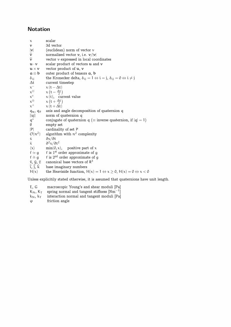
Notation

x scalarv 3d vector|v| (euclidean) norm of vector vv normalized vector v, i.e. v/|v|v vector v expressed in local coordinatesu · v scalar product of vectors u and v

u× v vector product of u, va⊗ b outer product of tensors a, bδij the Kronecker delta, δij = 1⇔ i = j, δij = 0⇔ i = j

∆t current timestepx− x (t− ∆t)x⊖ x

(t− ∆t

2

)x◦ x (t), current valuex⊕ x

(t+ ∆t

2

)x+ x (t+ ∆t)qu, qϑ axis and angle decomposition of quaternion q

||q|| norm of quaternion q

q∗ conjugate of quaternion q (≡ inverse quaternion, if |q| = 1)∅ empty set|P| cardinality of set PO(n2) algorithm with n2 complexityx ∂x/∂t

x ∂2x/∂t2

⟨x⟩ min(0, x), positive part of xf ≃ g f is 1st order approximate of gf ∼= g f is 2nd order approximate of gx, y, z canonical base vectors of R3

i, j, k base imaginary numbersH(x) the Heaviside function, H(x) = 1⇔ x ≥ 0, H(x) = 0⇔ x < 0

Unless explicitily stated otherwise, it is assumed that quaternions have unit length.

E, G macroscopic Young’s and shear moduli [Pa]KN, KT spring normal and tangent stiffness [Nm−1]kN, kT interaction normal and tangent moduli [Pa]φ friction angle

Introduction

This thesis is situated in the field of computational mechanics, which comprises mechanics, informaticsand programming.

The goal of the research project was modeling of massive fracturing of concrete at small scale duringhigh-rate processes. Traditional continuum-based modeling techniques, in particular the Finite ElementMethod (FEM), are designed (and efficient) for modeling continuum using discretization techniques, whilediscontinuities are introduced using relatively complicated extensions of the method (such as X-FEM).On the other hand, particle-based methods start from discrete entities and might obtain continuum-like behavior as an addition to the method. A discrete model with added continuous material featureswas chosen for our modeling task (rather than continuum-based model with added discontinuities), fordiscontinuous processes were predominant; because of high-rate effects, usage of a dynamic model wasdesirable. All those criteria led naturally to the Discrete Element Method (DEM) framework, in whichthe new concrete model (CPM, Concrete Particle Model) was formulated. This model was derived byapplying concepts from continuum mechanics (plasticity, damage, viscosity) onto discrete particles, whiletrying to assure appropriate continuous behavior of particle arrangements which are sufficiently large tosmear away individual particles.

As I spent the first year of PhD studies in Grenoble getting acquainted with Yade, a then-emergingopen-source software platform targeted mainly at DEM, it was naturally the platform chosen for theimplementation of the concrete model. Since my work on Yade during the first year concerned softwareengineering rather than mechanics, it was only later that I had to find out that Yade was not ready tobe used as-is for serious modeling, by only plugging a new model into it. Substantial changes had to bemade, which progressively covered all aspects of the program; that made me the lead developer of theYade project in the 2007–2010 period, focusing on usability, documentation and performance.

The thesis is divided in two parts.

The first part pertains to mechanics. The DEM itself is situated amongst other modeling techniques inchapter 1. Then, the DEM is formulated mathematically in chapter 2. Chapter 3 presents the concretemodel formulated in the DEM framework and implemented in Yade.

The second part is dedicated to Yade as software: it is presented from the point of view of a user and ofprogrammer. Generated documentation for Yade classes and modules is in appendices (C and D), as itis unlikely to be read as continuous text. Besides that, some classes were documented by their respectiveauthors and not me (see repository history for details); it is also for this reason that they are separatedfrom the main text body.

In order to make this thesis useful beyond its defense, most parts of this thesis are conceived as partof online Yade documentation at https://www.yade-dem.org/sphinx/. Automatically generated doc-umentation in appendices C and D is already part of it, while chapter 2 should become reference for thealgorithms in the future.

3

Part I.

Concrete particle model

5

1. Discrete Element Method

1.1. Characterisation

Usage of particle models for mechanical problems originated in geomechanics in 1979, in a famous paper byCundall & Strack named A discrete numerical model for granular assemblies [8]. Granular mediumis modeled in a discrete fashion: circular non-deformable particles representing granula can collide,exerting forces on one another, while being governed by Newton’s laws of dynamic equilibrium; theselaws are integrated using an explicit scheme, proceeding by a given ∆t at each step. Particles have bothtranslational and rotational degrees of freedom. Forces coming from collision of particles are computedusing penalty functions, which express simple spring-like contact, elastic in the normal sense (connectingboth spheres’ centers) and elasto-plastic with Mohr-Coulomb criterion in the perpendicular plane.

Since then, the initial formulation has been substantially enhanced in many ways, such as introduction ofnon-spherical particles, particle deformability, cohesion and fracturing. These features will be discussedlater, after we establish the distinction between the Discrete Element Method (DEM) and other particle-based methods; naturally, such classification is only operational and does not imply inexistence or evenimpossibility of various intermediate positions.

Mass-spring models, where nodes have only 3 degrees of freedom and their contacts only transmit normalforce. Mass is lumped into nodes without any associated volume, without collision detection andcreation of new contacts; initial contacts are pre-determined. Such models were used to model solidfracture (where dynamic effects were predominant [70]) or elastic cloth behavior [50].

Rigid body-spring model (RBSM), where polygonal/polyhedral particles are connected with multiplespring elements across the neighbor’s contact sides/areas; particles have no deformability on theirown, their elasticity is represented by said spring elements [27]; an implicit integration scheme isemployed. This method is similar to FEM with zero-thickness interface elements [4], but leads toa smaller stiffness matrix, since displacements of any point belonging to a particle are uniquelydetermined from displacements/rotations of the particle itself. Nagai et al. [41] uses elaborateplasticity functions for shear loading.

Lattice models family, where nodes are connected with truss or beam elements. Typically, nodes carryno mass and static equilibrium is sought; they do not occupy volume either, hence no new contactsbetween nodes will be created. Both regular and irregular lattices were studied. Properties ofconnecting elements are determined from local configuration, such as geometry of the Voronoï cellof each node and local material heterogeneity (e.g. mortar vs. aggregates in concrete).

Originally, lattice was representing elastic continuum; the equivalence was established for bothtruss [21] and beam [55] elements. Later, obvious enhancements such as brittle beam failure wereintroduced. Lattice models nicely show the emergence of relatively complex structural behavior,although fairly simple formulas govern local processes.

Some models find themselves on the border between DEM and lattice models, e.g. by consideringsphere packing for finding initial contacts, but only finding a static solution later [17].

7

1.2. Feature variations

This initial formulation has seen numerous improvements and enhancements since; we roughly follow thefeature classification in a nice overview by Bićanić [4].

1.2.1. Space dimension

Originally, 2d simulation space was used, as it reduces significantly computational costs. With theincrease of available computing power, the focus has shifted to 3d space. The number of dimensions alsoqualitatively influences some phenomena, such as dilation and percolation.

1.2.2. Particle geometry

Discs (2d) and spheres (3d) were first choices for the ease of contact detection, as sphere overlap isdetermined from spatial distance of their centroids, without the need to consider their orientation. Ap-proximating more complex shapes by spheres can be done by building up rigid aggregates (“clumps”),which might try to approximate real surfaces [49].

At further development stages, elliptical shapes, general quadrics and implicit superquadrics all havebeen used. The advantage is that, unlike for other complex shapes, the solid predicate (whether a givenpoint is inside or outside) is computed very fast; however, to detect collision of 2 such shapes, one particleis usually discretized into a set of surface points, and the predicate of the other particle is applied onthose points.

Polygons/polyhedra with explicit vertices are frequently used. Exact detection of contact might betricky and has to distinguish combinations of features that enter the interaction: edge-edge, vertex-edge,vertex-facet, etc.

Surface singularities at vertices can be problematic, since direction of the repulsive force (penalty function)is not clearly defined. Several solutions are employed: rounding edges and vertices, replacing them withaligned spheres and cylinders; formulating the penalty function volumetrically (e.g. in the directionof the least principal moment of inertia of the overlapping volume, which is the direction the volumewill decrease the fastest); using some more detailed knowledge about the particles in question, such astracking the common plane defined by arrangement of vertices and faces during movement of particles[43].

Arbitrary discrete functions have been employed for particle shapes as well.

1.2.3. Contact detection algorithm

Naïve checking of all possible couples soon leads to performance issues with increasing number of particles,having O(n2) complexity. Moreover, for complex shapes exact contact evaluation can be complicated.Therefore, the detection is generally done in 2 passes, the first one eliminating as many contacts aspossible:

1. Possible contacts based on approximate volume representation are sought; different particle geome-tries within the simulation do not have to be distinguished at this stage explicitly. Most non-trivialalgorithms are O(n logn), which makes them unusable for very large number of particles althoughO(n) algorithms were already published [38, 40].

2. Possible contacts are evaluated, considering the exact geometry of particles. In this pass, all possiblecombinations of shapes must be handled.

8

1.2.4. Boundary conditions

Boundaries can be imposed at space level or at particle level.

Space boundaries are, in particular, periodic boundaries, where particles leaving the periodic cell onone side enter on the other side; for the periodicity condition to hold, the cell must be parallelepiped-shaped. The periodic boundary eliminates boundary-related distortions of simulations; it also preventslocalization unless orientation of the cell matches that of the localization plane.

Particle-level boundaries may be as simple as fixing some particles in space; other boundaries, which aimat a more faithful representation of experimental setups, might be [4]

flexible where a chain of particles is tied together by links (keeping the circumference constant) or

hydrostatic where forces corresponding to constant hydrostatic stress are exerted on particles on theboundary.

In both cases, a definition of a particle “on the boundary” is needed; for spheres, Voronoï (Dirichlet)tessellation [3] might be used with weighting employed to account for different sphere radii.

1.2.5. Particle deformability

The initial Cundall’s formulation supposed that particles themselves are rigid (their geometry undergoesno changes) and it is only at the interaction level that elastic behavior occurs.

Early attempts at deformability considered discrete elements as deformable quadrilaterals (Bićanić [4]calls this method “discrete finite elements”). Several further development branches were followed later:

Combined finite/discrete element method (FDEM) [39, 37] discretizes each discrete element internallyinto multiple finite elements. Special care must be taken to account for the interplay between external(discrete element boundary), internal (finite element stresses) and inertial (mass) forces. By allowingfracturing inside the FEM domain, the discrete element can be effectively crushed and then fall apartinto multiple discrete elements. This method uses explicit integration and usual inter-particle contacthandling via penalty functions, distributing external forces onto surface FE nodes.

Discontinuous deformation analysis (DDA) [58] superimposes polynomial approximation of the strainfield on the movement of the rigid body centroid. Evolutions in this direction included increasing thepolynomial order as well as dividing the discrete element in a number of sub-blocks with a lower-degreepolynomial. Implicit integration is used, while taking contact constraints into account.

Non-rigid aggregates do not constitute a method on its own but account for deformable particlesby clustering primitive, rigid particles using a special type of cohesive bonds, creating a lattice-likedeformable solid representation.

1.2.6. Cohesion and fracturing

Cohesive interactions (“bonds”) between particles have been used to represent non-granular media. Iffracturing is to take place the formulation is usually derived from continuum elastic-plastic-damagemodels [4], though not necessarily [19]; such an approach only allows inter-particle fracture. Intra-particlefracture can be emulated with non-rigid aggregates or properly simulated in FDEM where localizationand remeshing of the originally continuous FEM domain allows progressive fracturing [37].

9

1.2.7. Time integration scheme

Integrating motion equations in discrete elements system needs special consideration. Penalty functionsexpressing repulsive forces (for cohesion-less setups) have some order of discontinuity when contact occurs.This favors explicit integration methods, which are indeed used in the most discrete element codes. Thenumerical stability criterion reads ∆t <

√m/k, where m is mass and k is contact stiffness; this equation

has physical meaning for corresponding continuum material, limiting distance of elastic wave propagationwithin one step, ∆x =

√E/ρ∆t, to the radius of spherical particle (∆x ≤ r).

In implicit integration schemes, global stiffness matrix is assembled and dynamic equilibrium is sought;this allows for larger ∆t values, but the computation is more complex. In DDA, to assure non-singularityof the matrix in the absence of contact between blocks, artificial low spring stiffness terms might have tobe added [4].

1.3. Micro-macro behavior relations

Although for reasons of an easier fracture description continuum may be represented by particles withspecial bonds in such way that desired macroscopic behavior is obtained, the correspondence of bond-level and domain-level properties is far from clear and has been the subject of considerable research. Thetwo levels are colloquially called micro and macro, although this bears no reference to “microscopic”scale as opposed to meso/macroscopic scale as otherwise used in material modeling.

Elastic properties (Young’s modulus E and Poisson’s ratio ν) already pose some problems as to whatvalues should be expected based on given micro-parameters: stiffnesses in the normal (KN) and shear(KT ) sense, in case of spherical DEM with 3-DoF contacts. It follows from dimensional analysis thatν = ν (KT/KN) and E = KNf(KT/KN). Analytical solutions of this problem start from either of thefollowing suppositions:

Regular lattice can be used for hand-derivation of macroscopic E and ν from bond-level strain-stressformulas. For 2D, the Potapov et al. [46] article derives macroscopic properties on 2 differentlyoriented hexagonal lattices and then shows they will converge when refined, making the limit valuevalid for any orientation; Potapov et al. [47] gives numerical evidence for the result. For 3D, Wangand Mora [69] derives equations on regular dense packing of spheres (hexagonal close-packed andface-centered cubic) using energy considerations.

General lattice. For the 3D case, the principle of energy conservation is used. External work (imposedvia homogeneous strain field) and potential energy (expressed as stored elastic energy of bonds)are equaled, resulting in closed-form solution for E and ν. This can be done in a discrete fashion(by summing bonds between particles) or using integral form of the imaginary continuous “lattice”.Such an approach is used by Liao et al. [34] and leads to integrals analogous to the microplanetheory; the analogy is explicitly used by Kuhl et al. [31] in the context of DEM.

Liao et al. [34] shows, however, that the general homogeneous strain field biases the result and pro-poses a “best-fit” strategy (in both a discrete and integral form), showing that the actual numericalresults are between the two; this is used, e.g., by Hentz et al. [20] for DEM-based concrete modelcalibration.

10

2. Problem formulation

In this chapter, we mathematically describe general features of explicit DEM simulations, with somereference to Yade implementation of these algorithms.

They are given roughly in the order as they appear in simulation; first, two particles might establish anew interaction, which consists in

1. detecting collision between particles;

2. creating new interaction and determining its properties (such as stiffness); they are either precom-puted or derived from properties of both particles;

Then, for already existing interactions, the following is performed:

1. strain evaluation;

2. stress computation based on strains;

3. force application to particles in interaction.

This simplified description serves only to give meaning to the ordering of sections within this chapter. Amore detailed description of this simulation loop is given later.

2.1. Collision detection

2.1.1. Generalities

Exact computation of collision configuration between two particles can be relatively expensive (for in-stance between Sphere and Facet). Taking a general pair of bodies i and j and their “exact”1 spatialpredicates (called Shape in Yade) represented by point sets Pi, Pj the detection generally proceeds in 2passes:

1. fast collision detection using approximate predicate Pi and Pj; they are pre-constructed in such away as to abstract away individual features of Pi and Pj and satisfy the condition

∀x ∈ R3 : x ∈ Pi ⇒ x ∈ Pi (2.1)(likewise for Pj). The approximate predicate is called “bounding volume” (Bound in Yade) since itbounds any particle’s volume from outside (by virtue of the implication). It follows that (Pi∩Pj) =∅⇒ (Pi ∩ Pj) = ∅ and, by applying modus tollens,(

Pi ∩ Pj

)= ∅⇒ (

Pi ∩ Pj

)= ∅ (2.2)

which is a candidate exclusion rule in the proper sense.

2. By filtering away impossible collisions in (2.2), more expensive, exact collision detection algorithmscan be run on possible interactions, filtering out remaining spurious couples (Pi∩Pj) = ∅∧

(Pi∩Pj

)=

∅. These algorithms operate on Pi and Pj and have to be able to handle all possible combinationsof shape types.

It is only the first step we are concerned with here.1 In the sense of precision admissible by numerical implementation.

11

2.1.2. Algorithms

Collision evaluation algorithms have been the subject of extensive research in fields such as robotics,computer graphics and simulations. They can be roughly divided in two groups:

Hierarchical algorithms which recursively subdivide space and restrict the number of approximate checksin the first pass, knowing that lower-level bounding volumes can intersect only if they are part of thesame higher-level bounding volume. Hierarchy elements are bounding volumes of different kinds:octrees [26], bounding spheres [22], k-DOP’s [28].

Flat algorithms work directly with bounding volumes without grouping them in hierarchies first; let usonly mention two kinds commonly used in particle simulations:

Sweep and prune algorithm operates on axis-aligned bounding boxes, which overlap if and onlyif they overlap along all axes. These algorithms have roughly O(n logn) complexity, where n isnumber of particles as long as they exploit temporal coherence of simulation (2.1.2).

Grid algorithms represent continuous R3 space by a finite set of regularly spaced points, leadingto very fast neighbor search; they can reach the O(n) complexity [38] and recent research suggestsways to overcome one of the major drawbacks of this method, which is the necessity to adjust gridcell size to the largest particle in the simulation (Munjiza et al. [40], the “multistep” extension).

Temporal coherence expresses the fact that motion of particles in simulation is not arbitrary butgoverned by physical laws. This knowledge can be exploited to optimize performance.

Numerical stability of integrating motion equations dictates an upper limit on ∆t (sect. 2.5.6) and, byconsequence, on displacement of particles during one step. This consideration is taken into account inMunjiza et al. [40], implying that any particle may not move further than to a neighboring grid cellduring one step allowing the O(n) complexity; it is also explored in the periodic variant of the sweepand prune algorithm described below.

On a finer level, it is common to enlarge Pi predicates in such a way that they satisfy the (2.1) conditionduring several timesteps; the first collision detection pass might then be run with stride, speeding upthe simulation considerably. The original publication of this optimization by Verlet [65] used enlargedlist of neighbors, giving this technique the name Verlet list. In general cases, however, where neighborlists are not necessarily used, the term Verlet distance is employed.

2.1.3. Sweep and prune

Let us describe in detail the sweep and prune algorithm used for collision detection in Yade (classInsertionSortCollider). Axis-aligned bounding boxes (Aabb) are used as Pi; each Aabb is given by lowerand upper corner ∈ R3 (in the following, Px0

i , Px1i are minimum/maximum coordinates of Pi along the

x-axis and so on). Construction of Aabb from various particle Shape’s (such as Sphere, Facet, Wall)is straightforward, handled by appropriate classes deriving form BoundFunctor (Bo1_Sphere_Aabb,Bo1_Facet_Aabb, …).

Presence of overlap of two Aabb’s can be determined from conjunction of separate overlaps of intervalsalong each axis (fig. 2.1):Ä

Pi ∩ Pj

ä= ∅⇔ ∧

w∈{x,y,z}

îÄÄPw0i , Pw1

i

ä∩ÄPw0j , Pw1

j

ää= ∅ó

(2.3)

where (a, b) denotes interval in R.

12

P1

P2P3

Px01

+x

+y

Px11

Px02

Px03

Px12

Px13

Py13

Py03

Py12

Py02

Py11

Py01

P3P2

P1

Figure 2.1.: Sweep and prune algorithm (shown in 2D), where Aabb of each sphere is represented byminimum and maximum value along each axis. Spatial overlap of Aabb’s is present if theyoverlap along all axes. In this case, P1 ∩ P2 = ∅ (but note that P1 ∩ P2 = ∅) and P2 ∩ P3 = ∅.

The collider keeps 3 separate lists (arrays) Lw for each axis w ∈ {x, y, z}

Lw =∪i

{Pw0i , Pw1

i

}(2.4)

where i traverses all particles. Lw arrays (sorted sets) contain respective coordinates of minimum andmaximum corners for each Aabb (we call these coordinates bound in the following); besides bound, eachof list elements further carries id referring to particle it belongs to, and a flag whether it is lower or upperbound.

In the initial step, all lists are sorted (using quicksort, average O(n logn)) and one axis is used to createinitial interactions: the range between lower and upper bound for each body is traversed, while boundsin-between indicate potential Aabb overlaps which must be checked on the remaining axes as well.

At each successive step, lists are already pre-sorted. Inversions occur where a particle’s coordinate hasjust crossed another particle’s coordinate; this number is limited by numerical stability of simulation andits physical meaning (giving spatio-temporal coherence to the algorithm). The insertion sort algorithmswaps neighboring elements if they are inverted, and has complexity between O(n) and O(n2), for pre-sorted and unsorted lists respectively. For our purposes, we need only to handle inversions, which bynature of the sort algorithm are detected inside the sort loop. An inversion might signify:

• New overlap along the current axis, if an upper bound inverts (swaps) with a lower bound (i.e.that the upper bound with a higher coordinate was out of order in coming before the lower boundwith a lower coordinate). Overlap along the other 2 axes is checked and if there is overlap alongall axes, a new potential interaction is created.

• End of overlap along the current axis, if lower bound inverts (swaps) with an upper bound. If thereis only potential interaction between the two particles in question, it is deleted.

• Nothing if both bounds are upper or both lower.

2.1.3.1. Aperiodic insertion sort

Let us show the sort algorithm on a sample sequence of numbers:

|| 3 7 2 4 || (2.5)

13

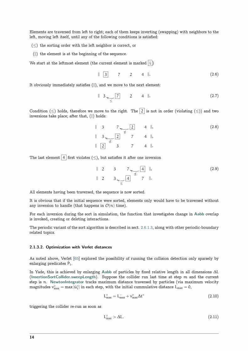
Elements are traversed from left to right; each of them keeps inverting (swapping) with neighbors to theleft, moving left itself, until any of the following conditions is satisfied:

(≤) the sorting order with the left neighbor is correct, or

(||) the element is at the beginning of the sequence.

We start at the leftmost element (the current element is marked i )

|| 3 7 2 4 ||. (2.6)

It obviously immediately satisfies (||), and we move to the next element:

|| 3 7≤

gg 2 4 ||. (2.7)

Condition (≤) holds, therefore we move to the right. The 2 is not in order (violating (≤)) and twoinversions take place; after that, (||) holds:

|| 3 7 2≤

hh 4 ||,

|| 3 2≤

hh 7 4 ||,

|| 2 3 7 4 ||.

(2.8)

The last element 4 first violates (≤), but satisfies it after one inversion

|| 2 3 7 4≤

hh ||,

|| 2 3 4≤

gg 7 ||.

(2.9)

All elements having been traversed, the sequence is now sorted.

It is obvious that if the initial sequence were sorted, elements only would have to be traversed withoutany inversion to handle (that happens in O(n) time).

For each inversion during the sort in simulation, the function that investigates change in Aabb overlapis invoked, creating or deleting interactions.

The periodic variant of the sort algorithm is described in sect. 2.6.1.3, along with other periodic-boundaryrelated topics.

2.1.3.2. Optimization with Verlet distances

As noted above, Verlet [65] explored the possibility of running the collision detection only sparsely byenlarging predicates Pi.

In Yade, this is achieved by enlarging Aabb of particles by fixed relative length in all dimensions ∆L

(InsertionSortCollider.sweepLength). Suppose the collider run last time at step m and the currentstep is n. NewtonIntegrator tracks maximum distance traversed by particles (via maximum velocitymagnitudes v◦max = max |u◦

i | in each step, with the initial cummulative distance Lmax = 0,

L◦max = L−max + v◦max∆t◦ (2.10)

triggering the collider re-run as soon as

L◦max > ∆L. (2.11)

14

The disadvantage of this approach is that even one fast particle determines v◦max.

A solution is to track maxima per particle groups. The possibility of tracking each particle separately(that is what ESyS-Particle [14] does) seemed to us too fine-grained. Instead, we assign particles tobn (InsertionSortCollider.nBins) velocity bins based on their current velocity magnitude. The bins’limit values are geometrical with the coefficient bc > 1 (InsertionSortCollider.binCoeff), the maximumvelocity being the current global velocity maximum v◦max (with some constraints on its change rate, toavoid large oscillations); for bin i ∈ {0, . . . , bn} and particle j:

v◦maxb−(i+1)c ≤ |u◦

j | < vmaxb−ic . (2.12)

(note that in this case, superscripts of bc mean exponentiation). Equations (2.10)–(2.11) are used for eachbin separately; however, when (2.11) is satisfied, full collider re-run is necessary and all bins’ distancesare reset.

Particles in high-speed oscillatory motion could be put into a slow bin if they happen to be at the pointwhere their instantaneous speed is low, causing the necessity of early collider re-run. This is avoided byallowing particles to only go slower by one bin rather than several at once.

Results of using Verlet distance depend highly on the nature of simulation and choice of parametersInsertionSortCollider.nBins and InsertionSortColldier.binCoeff. The binning algorithm was specificallydesigned for simulating local fracture of larger concrete specimen; in that way, only particles in thefracturing zone, with greater velocities, had the Aabb’s enlarged, without affecting quasi-still particlesoutside of this zone. In such cases, up to 50% overall computation time savings were observed, colliderbeing run every ≈100 steps in average.

2.2. Creating interaction between particles

Collision detection described above is only approximate. Exact collision detection depends on the ge-ometry of individual particles and is handled separately. In Yade terminology, the Collider creates onlypotential interactions; potential interactions are evaluated exactly using specialized algorithms for colli-sion of two spheres or other combinations. Exact collision detection must be run at every timestep sinceit is at every step that particles can change their mutual position (the collider is only run sometimes ifthe Verlet distance optimization is in use). Some exact collision detection algorithms are described insect. 2.3; in Yade, they are implemented in classes deriving from InteractionGeometryFunctor (prefixedwith Ig2).

Besides detection of geometrical overlap (which corresponds to InteractionGeometry in Yade), there arealso non-geometrical properties of the interaction to be determined (InteractionPhysics). In Yade, theyare computed for every new interaction by calling a functor deriving from InteractionPhysicsFunctor(prefixed with Ip2) which accepts the given combination of Material types of both particles.

2.2.1. Stiffnesses

Basic DEM interaction defines two stiffnesses: normal stiffness KN and shear (tangent) stiffness KT .It is desirable that KN be related to fictitious Young’s modulus of the particles’ material, while KT istypically determined as a given fraction of computed KN. The KT/KN ratio determines macroscopicPoisson’s ratio of the arrangement, which can be shown by dimensional analysis: elastic continuum hastwo parameters (E and ν) and basic DEM model also has 2 parameters with the same dimensions KN andKT/KN; macroscopic Poisson’s ratio is therefore determined solely by KT/KN and macroscopic Young’smodulus is then proportional to KN and affected by KT/KN.

Naturally, such analysis is highly simplifying and does not account for particle radius distribution, packingconfiguration and other possible parameters such as the interaction radius introduced later.

15

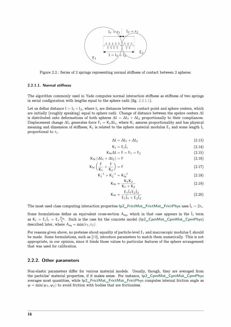
E1

E2

l1 = r1 l2 = r2

l = l1 + l2

Figure 2.2.: Series of 2 springs representing normal stiffness of contact between 2 spheres.

2.2.1.1. Normal stiffness

The algorithm commonly used in Yade computes normal interaction stiffness as stiffness of two springsin serial configuration with lengths equal to the sphere radii (fig. 2.2.1.1).

Let us define distance l = l1+ l2, where li are distances between contact point and sphere centers, whichare initially (roughly speaking) equal to sphere radii. Change of distance between the spehre centers ∆lis distributed onto deformations of both spheres ∆l = ∆l1 + ∆l2 proportionally to their compliances.Displacement change ∆li generates force Fi = Ki∆li, where Ki assures proportionality and has physicalmeaning and dimension of stiffness; Ki is related to the sphere material modulus Ei and some length liproportional to ri.

∆l = ∆l1 + ∆l2 (2.13)Ki = Eili (2.14)

KN∆l = F = F1 = F2 (2.15)KN (∆l1 + ∆l2) = F (2.16)

KN

ÅF

K1

+F

K2

ã= F (2.17)

K−11 + K−1

2 = K−1N (2.18)

KN =K1K2

K1 + K2

(2.19)

KN =E1l1E2l2

E1l1 + E2l2(2.20)

The most used class computing interaction properties Ip2_FrictMat_FrictMat_FrictPhys uses li = 2ri.

Some formulations define an equivalent cross-section Aeq, which in that case appears in the li termas Ki = Eili = Ei

Aeqli

. Such is the case for the concrete model (Ip2_CpmMat_CpmMat_CpmPhys)described later, where Aeq = min(r1, r2).

For reasons given above, no pretense about equality of particle-level Ei and macroscopic modulus E shouldbe made. Some formulations, such as [19], introduce parameters to match them numerically. This is notappropriate, in our opinion, since it binds those values to particular features of the sphere arrangementthat was used for calibration.

2.2.2. Other parameters

Non-elastic parameters differ for various material models. Usually, though, they are averaged fromthe particles’ material properties, if it makes sense. For instance, Ip2_CpmMat_CpmMat_CpmPhysaverages most quantities, while Ip2_FrictMat_FrictMat_FrictPhys computes internal friction angle asφ = min(φ1, φ2) to avoid friction with bodies that are frictionless.

16

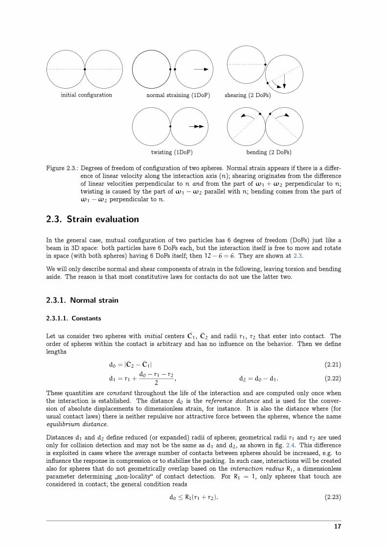
initial configuration

twisting (1DoF)

normal straining (1DoF) shearing (2 DoFs)

bending (2 DoFs)

Figure 2.3.: Degrees of freedom of configuration of two spheres. Normal strain appears if there is a differ-ence of linear velocity along the interaction axis (n); shearing originates from the differenceof linear velocities perpendicular to n and from the part of ω1 + ω2 perpendicular to n;twisting is caused by the part of ω1 −ω2 parallel with n; bending comes from the part ofω1 −ω2 perpendicular to n.

2.3. Strain evaluation

In the general case, mutual configuration of two particles has 6 degrees of freedom (DoFs) just like abeam in 3D space: both particles have 6 DoFs each, but the interaction itself is free to move and rotatein space (with both spheres) having 6 DoFs itself; then 12− 6 = 6. They are shown at 2.3.

We will only describe normal and shear components of strain in the following, leaving torsion and bendingaside. The reason is that most constitutive laws for contacts do not use the latter two.

2.3.1. Normal strain

2.3.1.1. Constants

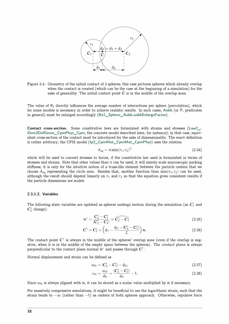
Let us consider two spheres with initial centers C1, C2 and radii r1, r2 that enter into contact. Theorder of spheres within the contact is arbitrary and has no influence on the behavior. Then we definelengths

d0 = |C2 − C1| (2.21)

d1 = r1 +d0 − r1 − r2

2, d2 = d0 − d1. (2.22)

These quantities are constant throughout the life of the interaction and are computed only once whenthe interaction is established. The distance d0 is the reference distance and is used for the conver-sion of absolute displacements to dimensionless strain, for instance. It is also the distance where (forusual contact laws) there is neither repulsive nor attractive force between the spheres, whence the nameequilibrium distance.

Distances d1 and d2 define reduced (or expanded) radii of spheres; geometrical radii r1 and r2 are usedonly for collision detection and may not be the same as d1 and d2, as shown in fig. 2.4. This differenceis exploited in cases where the average number of contacts between spheres should be increased, e.g. toinfluence the response in compression or to stabilize the packing. In such case, interactions will be createdalso for spheres that do not geometrically overlap based on the interaction radius RI, a dimensionlessparameter determining „non-locality“ of contact detection. For RI = 1, only spheres that touch areconsidered in contact; the general condition reads

d0 ≤ RI(r1 + r2). (2.23)

17

d0 = d1 + d2

C2C1

d1 d2

r1

r2

C

Figure 2.4.: Geometry of the initial contact of 2 spheres; this case pictures spheres which already overlapwhen the contact is created (which can be the case at the beginning of a simulation) for thesake of generality. The initial contact point C is in the middle of the overlap zone.

The value of RI directly influences the average number of interactions per sphere (percolation), whichfor some models is necessary in order to achieve realistic results. In such cases, Aabb (or Pi predicatesin general) must be enlarged accordingly (Bo1_Sphere_Aabb.aabbEnlargeFactor).

Contact cross-section. Some constitutive laws are formulated with strains and stresses (Law2_-Dem3DofGeom_CpmPhys_Cpm, the concrete model described later, for instance); in that case, equiv-alent cross-section of the contact must be introduced for the sake of dimensionality. The exact definitionis rather arbitrary; the CPM model (Ip2_CpmMat_CpmMat_CpmPhys) uses the relation

Aeq = πmin(r1, r2)2 (2.24)

which will be used to convert stresses to forces, if the constitutive law used is formulated in terms ofstresses and strains. Note that other values than π can be used; it will merely scale macroscopic packingstiffness; it is only for the intuitive notion of a truss-like element between the particle centers that wechoose Aeq representing the circle area. Besides that, another function than min(r1, r2) can be used,although the result should depend linearly on r1 and r2 so that the equation gives consistent results ifthe particle dimensions are scaled.

2.3.1.2. Variables

The following state variables are updated as spheres undergo motion during the simulation (as C◦1 and

C◦2 change):

n◦ =C◦

2 −C◦1

|C◦2 −C◦

1|≡ ÿ�C◦

2 −C◦1 (2.25)

C◦ = C◦1 +

Åd1 −

d0 − |C◦2 −C◦

1|

2

ãn. (2.26)

The contact point C◦ is always in the middle of the spheres’ overlap zone (even if the overlap is neg-ative, when it is in the middle of the empty space between the spheres). The contact plane is alwaysperpendicular to the contact plane normal n◦ and passes through C◦.

Normal displacement and strain can be defined as

uN = |C◦2 −C◦

1|− d0, (2.27)

εN =uN

d0

=|C◦

2 −C◦1|

d0

− 1. (2.28)

Since uN is always aligned with n, it can be stored as a scalar value multiplied by n if necessary.

For massively compressive simulations, it might be beneficial to use the logarithmic strain, such that thestrain tends to −∞ (rather than −1) as centers of both spheres approach. Otherwise, repulsive force

18

uT

C

n

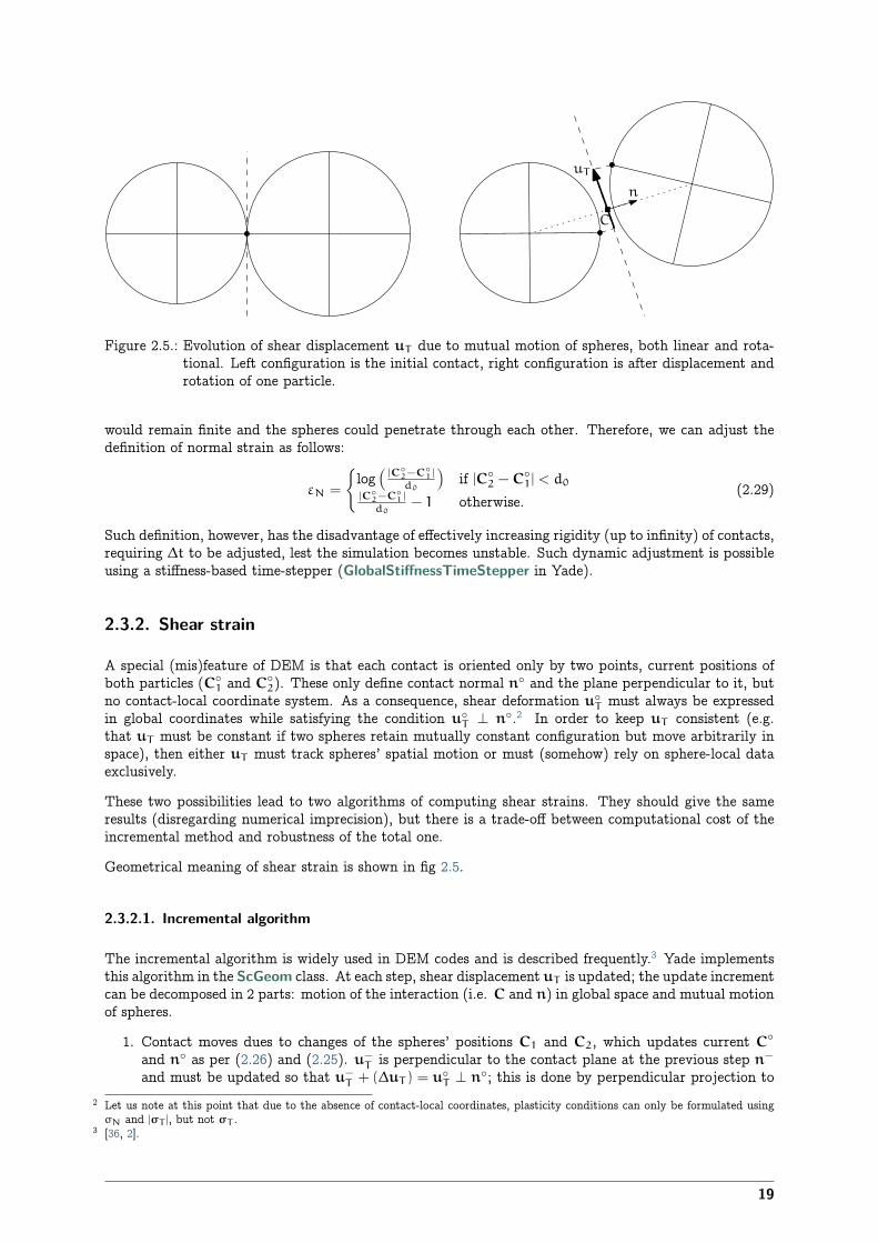
Figure 2.5.: Evolution of shear displacement uT due to mutual motion of spheres, both linear and rota-tional. Left configuration is the initial contact, right configuration is after displacement androtation of one particle.

would remain finite and the spheres could penetrate through each other. Therefore, we can adjust thedefinition of normal strain as follows:

εN =

{logÄ|C◦

2−C◦1|

d0

äif |C◦

2 −C◦1| < d0

|C◦2−C◦

1|

d0− 1 otherwise.

(2.29)

Such definition, however, has the disadvantage of effectively increasing rigidity (up to infinity) of contacts,requiring ∆t to be adjusted, lest the simulation becomes unstable. Such dynamic adjustment is possibleusing a stiffness-based time-stepper (GlobalStiffnessTimeStepper in Yade).

2.3.2. Shear strain

A special (mis)feature of DEM is that each contact is oriented only by two points, current positions ofboth particles (C◦

1 and C◦2). These only define contact normal n◦ and the plane perpendicular to it, but

no contact-local coordinate system. As a consequence, shear deformation u◦T must always be expressed

in global coordinates while satisfying the condition u◦T ⊥ n◦.2 In order to keep uT consistent (e.g.

that uT must be constant if two spheres retain mutually constant configuration but move arbitrarily inspace), then either uT must track spheres’ spatial motion or must (somehow) rely on sphere-local dataexclusively.

These two possibilities lead to two algorithms of computing shear strains. They should give the sameresults (disregarding numerical imprecision), but there is a trade-off between computational cost of theincremental method and robustness of the total one.

Geometrical meaning of shear strain is shown in fig 2.5.

2.3.2.1. Incremental algorithm

The incremental algorithm is widely used in DEM codes and is described frequently.3 Yade implementsthis algorithm in the ScGeom class. At each step, shear displacement uT is updated; the update incrementcan be decomposed in 2 parts: motion of the interaction (i.e. C and n) in global space and mutual motionof spheres.

1. Contact moves dues to changes of the spheres’ positions C1 and C2, which updates current C◦

and n◦ as per (2.26) and (2.25). u−T is perpendicular to the contact plane at the previous step n−

and must be updated so that u−T + (∆uT ) = u◦

T ⊥ n◦; this is done by perpendicular projection to2 Let us note at this point that due to the absence of contact-local coordinates, plasticity conditions can only be formulated using

σN and |σT |, but not σT .3 [36, 2].

19

the plane first (which might decrease |uT |) and adding what corresponds to spatial rotation of theinteraction instead:

(∆uT )1 = −u−T × (n− × n◦) (2.30)

(∆uT )2 = −u−T ×Å∆t

2n◦ · (ω⊖

1 +ω⊖2 )

ãn◦ (2.31)

2. Mutual movement of spheres, using only its part perpendicular to n◦; v12 denotes mutual velocityof spheres at the contact point:

v12 =(v⊖2 +ω−

2 × (−d2n◦))−(v⊖1 +ω⊖

1 × (d1n◦))

(2.32)v⊥12 = v12 − (n◦ · v12)n◦ (2.33)

(∆uT )3 = −∆tv⊥12 (2.34)

Finally, we computeu◦T = u−

T + (∆uT )1 + (∆uT )2 + (∆uT )3. (2.35)

2.3.2.2. Total alogithm

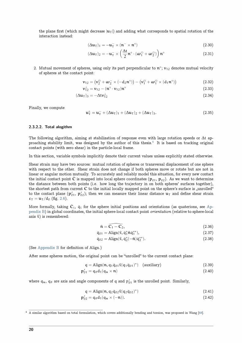
The following algorithm, aiming at stabilization of response even with large rotation speeds or ∆t ap-proaching stability limit, was designed by the author of this thesis.4 It is based on tracking originalcontact points (with zero shear) in the particle-local frame.

In this section, variable symbols implicitly denote their current values unless explicitly stated otherwise.

Shear strain may have two sources: mutual rotation of spheres or transversal displacement of one spherewith respect to the other. Shear strain does not change if both spheres move or rotate but are not inlinear or angular motion mutually. To accurately and reliably model this situation, for every new contactthe initial contact point C is mapped into local sphere coordinates (p01, p02). As we want to determinethe distance between both points (i.e. how long the trajectory in on both spheres’ surfaces together),the shortest path from current C to the initial locally mapped point on the sphere’s surface is „unrolled“to the contact plane (p ′

01, p ′02); then we can measure their linear distance uT and define shear strain

εT = uT/d0 (fig. 2.6).

More formally, taking Ci, qi for the sphere initial positions and orientations (as quaterions, see Ap-pendix B) in global coordinates, the initial sphere-local contact point orientation (relative to sphere-localaxis x) is remembered:

n = ÿ�C1 −C2, (2.36)q01 = Align(x, q∗

1nq∗∗1 ), (2.37)

q02 = Align(x, q∗2(−n)q∗∗

2 ). (2.38)

(See Appendix B for definition of Align.)

After some spheres motion, the original point can be “unrolled” to the current contact plane:

q = Align(n, q1q01x(q1q01)∗) (auxiliary) (2.39)

p ′01 = qϑd1(qu × n) (2.40)

where qu, qϑ are axis and angle components of q and p ′01 is the unrolled point. Similarly,

q = Align(n, q2q02x(q2q02)∗) (2.41)

p ′02 = qϑd1(qu × (−n)). (2.42)

4 A similar algorithm based on total formulation, which covers additionally bending and torsion, was proposed in Wang [68].

20

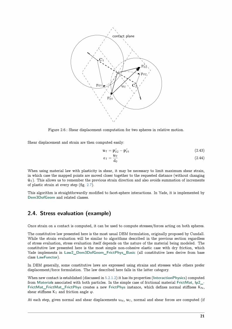
C1

C2

p02

p01

p ′01

p ′02

uT

contact plane

Figure 2.6.: Shear displacement computation for two spheres in relative motion.

Shear displacement and strain are then computed easily:

uT = p ′02 − p ′

01 (2.43)

εT =uT

d0

(2.44)

When using material law with plasticity in shear, it may be necessary to limit maximum shear strain,in which case the mapped points are moved closer together to the requested distance (without changinguT ). This allows us to remember the previous strain direction and also avoids summation of incrementsof plastic strain at every step (fig. 2.7).

This algorithm is straightforwardly modified to facet-sphere interactions. In Yade, it is implemented byDem3DofGeom and related classes.

2.4. Stress evaluation (example)

Once strain on a contact is computed, it can be used to compute stresses/forces acting on both spheres.

The constitutive law presented here is the most usual DEM formulation, originally proposed by Cundall.While the strain evaluation will be similar to algorithms described in the previous section regardlessof stress evaluation, stress evaluation itself depends on the nature of the material being modeled. Theconstitutive law presented here is the most simple non-cohesive elastic case with dry friction, whichYade implements in Law2_Dem3DofGeom_FrictPhys_Basic (all constitutive laws derive from baseclass LawFunctor).

In DEM generally, some constitutive laws are expressed using strains and stresses while others preferdisplacement/force formulation. The law described here falls in the latter category.

When new contact is established (discussed in 5.2.1.2) it has its properties (InteractionPhysics) computedfrom Materials associated with both particles. In the simple case of frictional material FrictMat, Ip2_-FrictMat_FrictMat_FrictPhys creates a new FrictPhys instance, which defines normal stiffness KN,shear stiffness KT and friction angle φ.

At each step, given normal and shear displacements uN, uT , normal and shear forces are computed (if

21

contact plane

C1

C2

requestedmax |uT |

old p01

old p02

p01

p02

p ′01

p ′02

old p ′01

old p ′02

uT

Figure 2.7.: Shear plastic slip for two spheres.

uN > 0, the contact is deleted without generating any forces):

FN = KNuNn, (2.45)FtT = KTuT (2.46)

where FN is normal force and FT is trial shear force. A simple non-associated stress return algorithm isapplied to compute final shear force

FT =

{FtT

|FN| tanφ

FtT

if |FT | > |FN| tanφ,

FtT otherwise.(2.47)

Summary force F = FN + FT is then applied to both particles – each particle accumulates forces andtorques acting on it in the course of each step. Because the force computed acts at contact point C,which is difference from sphes’ centers, torque generated by F must also be considered.

F1+ = F F2+ = −F (2.48)T1+ = d1(−n)× F T2+ = d2n× F. (2.49)

2.5. Motion integration

Each particle accumulates generalized forces (forces and torques) from the contacts in which it partici-pates. These generalized forces are then used to integrate motion equations for each particle separately;therefore, we omit i indices denoting the i-th particle in this section.

The customary leapfrog scheme (also known as the Verlet scheme) is used, with some adjustments forrotation of non-spherical particles, as explained below. The “leapfrog” name comes from the fact thateven derivatives of position/orientation are known at on-step points, whereas odd derivatives are knownat mid-step points. Let us recall that we use a−, a◦, a+ for on-step values of a at t − ∆t, t and t + ∆t

respectively; and a⊖, a⊕ for mid-step values of a at t− ∆t/2, t+ ∆t/2.

Described integration algorithms are implemented in the NewtonIntegrator class in Yade.

22

2.5.1. Position

Integrating motion consists in using current acceleration u◦ on a particle to update its position from the

current value u◦ to its value at the next timestep u+. Computation of acceleration, knowing currentforces F acting on the particle in question and its mass m, is simply

u◦ = F/m. (2.50)

Using the 2nd order finite difference with step ∆t, we obtain

u◦ ∼=

u− − 2u◦ + u+

∆t2(2.51)

from which we express

u+ = 2u◦ − u− + u◦∆t2 =

= u◦ + ∆t

Åu◦ − u−

∆t+ u◦

∆t

ã︸ ︷︷ ︸

(†)

. (2.52)

Typically, u− is already not known (only u◦ is); we notice, however, that

u⊖ ≃ u◦ − u−

∆t, (2.53)

i.e. the mean velocity during the previous step, which is known. Plugging this approximate into the (†)term, we also notice that mean velocity during the current step can be approximated as

u⊕ ≃ u

⊖ + u◦∆t, (2.54)

which is (†); we arrive finally at

u+ = u◦ + ∆tÄu⊖ + u

◦∆tä. (2.55)

The algorithm can then be written down by first computing current mean velocity u⊕ which we need tostore for the next step (just as we use its old value u

⊖ now), then computing the position for the nexttime step u+:

u⊕ = u⊖ + u◦∆t, (2.56)

u+ = u◦ + u⊕∆t. (2.57)

Positions are known at times i∆t (if ∆t is constant) while velocities are known at i∆t+ ∆t2. The facet that

they interleave (jump over each other) in such way gave rise to the colloquial name “leapfrog” scheme.

2.5.2. Orientation (spherical)

Updating particle orientation q◦ proceeds in an analogous way to position update. First, we computecurrent angular acceleration ω

◦ from known current torque T . For spherical particles where the inertiatensor is diagonal in any orientation (therefore also in current global orientation), satisfying I11 = I22 =I33, we can write

ω◦i = T i/I11, (2.58)

We use the same approximation scheme, obtaining an equation analogous to (2.56)

ω⊕ = ω⊖ + ∆tω◦. (2.59)

23

The quaternion (see Appendix B) ∆q representing rotation vector ω⊕∆t is constructed, i.e. such that

(∆q)ϑ = |ω⊕|, (2.60)(∆q)u = ω⊕ (2.61)

Finally, we compute the next orientation q+ by rotation composition

q+ = ∆qq◦. (2.62)

2.5.3. Orientation (aspherical)

Integrating rotation of aspherical particles is considerably more complicated than their position, as theirlocal reference frame is not inertial. Rotation of rigid body in the local frame, where inertia matrix I isdiagonal, is described in the continuous form by Euler’s equations (i ∈ {1, 2, 3} and i, j, k are subsequentindices):

T i = Iiiωi + (Ikk − Ijj)ωjωk. (2.63)Due to the presence of the current values of both ω and ω, they cannot be solved using the standardleapfrog algorithm (that was the case for translational motion and also for the spherical bodies’ rotationwhere this equation reduced to T = Iω).

The algorithm presented here is described by Allen and Tildesley [1, pg. 84–89] and was designed by Fin-cham for molecular dynamics problems; it is based on extending the leapfrog algorithm by mid-step/on-step estimators of quantities known at on-step/mid-step points in the basic formulation. Although it hasreceived criticism and more precise algorithms are known (Omelyan [44], Neto and Bellucci [42], Johnsonet al. [25]), this one is currently implemented in Yade for its relative simplicity.

Each body has its local coordinate system based on the principal axes of inertia for that body. We use • todenote vectors in local coordinates. The orientation of the local system is given by the current particle’sorientation q◦ as a quaternion; this quaternion can be expressed as the (current) rotation matrix A.Therefore, every vector a is transformed as a = qaq∗ = Aa. Since A is a rotation (orthogonal) matrix,the inverse rotation A−1 = AT .

For given particle in question, we know

I◦ (constant) inertia matrix; diagonal, since in local, principal coordinates,

T◦ external torque,

q◦ current orientation (and its equivalent rotation matrix A),

ω⊖ mid-step angular velocity,

L⊖ mid-step angular momentum; this is an auxiliary variable that must be tracked in addition for usein this algorithm. It will be zero in the initial step.

Our goal is to compute new values of the latter three, that is L⊕, q+, ω⊕. We first estimate currentangular momentum and compute current local angular velocity:

L◦ = L⊖ + T ◦∆t

2, L

◦= AL◦, (2.64)

L⊕ = L⊖ + T ◦∆t, L⊕= AL⊕, (2.65)‹ω◦

= I◦−1L◦, (2.66)‹ω⊕

= I◦−1L⊕. (2.67)

(2.68)

24

Then we compute q◦, using q◦ and ‹ω◦:Üq◦w

q◦x

q◦y

q◦z

ê=

1

2

Üq◦w −q◦

x −q◦y −q◦

z

q◦x q◦

w −q◦z q◦

y

q◦y q◦

z q◦w −q◦

x

q◦z −q◦

y q◦x q◦

w

êÜ0‹ω◦x‹ω◦y‹ω◦z

ê, (2.69)

q⊕ = q◦ + q◦∆t

2. (2.70)

We evaluate q⊕ from q⊕ and ‹ω⊕ in the same way as in (2.69) but shifted by ∆t/2 ahead. Then we canfinally compute the desired values

q+ = q◦ + q⊕∆t, (2.71)ω⊕ = A−1‹ω⊕ (2.72)

2.5.4. Clumps (rigid aggregates)

DEM simulations frequently make use of rigid aggregates of particles to model complex shapes [49] calledclumps, typically composed of many spheres. Dynamic properties of clumps are computed from theproperties of its members: the clump’s mass mc is summed over members, the inertia tensor Ic withrespect to the clump’s centroid is computed using the parallel axes theorem; local axes are oriented suchthat they are principal and inertia tensor is diagonal and clump’s orientation is changed to compensaterotation of the local system, as to not change the clump members’ positions in global space. Initialpositions and orientations of all clump members in local coordinate system are stored.

In Yade (class Clump), clump members behave as stand-alone particles during simulation for purposes ofcollision detection and contact resolution, except that they have no contacts created among themselveswithin one clump. It is at the stage of motion integration that they are treated specially. Instead of inte-grating each of them separately, forces/torques on those particles Fi, T i are converted to forces/torqueson the clump itself. Let us denote ri relative position of each particle with regards to clump’s centroid,in global orientation. Then summary force and torque on the clump are

Fc =∑

Fi/mc, (2.73)

Tc =∑

ri × Fi + Ti. (2.74)

Motion of the clump is then integrated, using aspherical rotation integration. Afterwards, clump membersare displaced in global space, to keep their initial positions and orientations in the clump’s local coordinatesystem. In such a way, relative positions of clump members are always the same, resulting in the behaviorof a rigid aggregate.

2.5.5. Numerical damping

In simulations of quasi-static phenomena, it it desirable to dissipate kinetic energy of particles. Sincemost constitutive laws (including Law_ScGeom_FrictPhys_Basic shown above, sect. 2.4) do not includevelocity-based damping (such as one in D’Addetta et al. [10]), it is possible to use artificial numericaldamping. The formulation is described in ICG [23], although our version is slightly adapted. The basicidea is to decrease forces which increase the particle velocities and vice versa by (∆F)d, comparing thecurrent acceleration sense and particle velocity sense. This is done by component, which makes thedamping scheme clearly non-physical, as it is not invariant with respect to coordinate system rotation;on the other hand, it is very easy to compute. Cundall proposed the form (we omit particle indices i

since it applies to all of them separately):

(∆F)dwFw

= −λd sgn(Fwu⊖w), w ∈ {x, y, z} (2.75)

where λd is the damping coefficient. This formulation has several advantages [19]:

25

• it acts on forces (accelerations), not constraining uniform motion;

• it is independent of eigenfrequencies of particles, they will be all damped equally;

• it needs only the dimensionless parameter λd which does not have to be scaled.

In Yade, we use the adapted form

(∆F)dwFw

= −λd sgn FwÅu⊖w +

u◦w∆t

2

ã︸ ︷︷ ︸

≃u◦w

, (2.76)

where we replaced the previous mid-step velocity u⊖ by its on-step estimate in parentheses. This is toavoid locked-in forces that appear if the velocity changes its sign due to force application at each step,i.e. when the particle in question oscillates around the position of equilibrium with 2∆t period.

In Yade, damping (2.76) is implemented in the NewtonIntegrator engine; the damping coefficient λd isNewtonIntegrator.damping.

2.5.6. Stability considerations

The leapfrog integration scheme is conditionally stable, i.e. not magnifying errors, provided ∆t < ∆tcrwhere ∆tcr is the critical timestep, above which the integration is unstable. Usually, ∆t is taken as afraction of ∆tcr; this fraction is called the timestep safety factor, with meaningful values ∈ ⟨0, 1).

2.5.6.1. Critical timestep (translational)

In order to ensure stability for the explicit integration sceheme, an upper limit is imposed on ∆t:

∆tcr =2

ωmax(2.77)

where ωmax is the highest angular eigenfrequency within the system.

Single mass-spring system with mass m and stiffness K is governed by the equation

mx = −Kx, (2.78)

where x is displacement from the mean (equilibrium) position. The solution of harmonic oscillation isx(t) = A cos(ωt+φ) where phase φ and amplitude A are determined by initial conditions. The angularfrequency

ω(1) =

…m

K(2.79)

does not depend on initial conditions. Since there is one single mass, ω(1)max = ω(1). Plugging (2.79) into

(2.77), we obtain∆t

(1)cr = 2/ω

(1)max = 2

»K/m (2.80)

for a single oscillator.

In general mass-spring system, the highest frequency occurs if two connected masses mi, mj are inopposite motion; let us suppose they have equal velocities (which is conservative) and they are connectedby a spring with stiffness Ki: displacement ∆xi of mi will be accompained by ∆xj = −∆xi of mj, giving∆Fi = −Ki(∆xi − (−∆xi)) = −2Ki∆xi. That results in apparent stiffness K

(2)i = 2Ki, giving maximum

angular frequency of the whole system

ωmax = maxi

√K(2)i /mi. (2.81)

26

The overall critical timestep is then

∆tcr =2

ωmax= min

i2

 mi

K(2)i

= mini

2

…mi

2Ki

= mini

√2

…mi

Ki

. (2.82)

This equation can be used in R3 simulations by evaluating the critical timestep per-axis and requiring

∆tcr = min∆tcrw, w ∈ {x, y, z}. (2.83)

In DEM simulations, per-particle stiffness Ki is determined from the stiffnesses of contacts in whichit participates [7]. Suppose each contact has normal stiffness KNj, shear stiffness KTj = ξKNj and isoriented by normal nj. Ki is then sum of contributions of all contacts in which it participates (indicesj), with terms along axes equal to

Kiw =∑j

(KNj − KTj)n2jw + KTj =

∑j

KNj

((1− ξ)n2

jw + ξ)

(2.84)

with w ∈ {x, y, z}. Equations (2.82), (2.83) and (2.84) determine ∆tcr in a simulation; it is implementedby the GlobalStiffnessTimeStepper engine in Yade.

This approach is simplifying, since only translational terms of the stiffness matrix are considered (which isthe limiting factor typically) and eigenvalues are estimated from diagonal terms only. Rigorous derivationof critical timestep is possible from overall stiffness and mass matrices; we have to leave it for posterityat this place, for time constraints.

There is one important condition that ωmax > 0: if there are no contacts between particles and ωmax = 0,we would obtain value ∆tcr = ∞. While formally correct, this value is numerically erroneous: we weresilently supposing that stiffness remains constant during each timestep, which is not true if contacts arecreated as particles collide. In case of no contact, therefore, stiffness must be pre-estimated based onfuture interactions, as shown in the next section.

2.5.6.2. Estimation of ∆tcr by wave propagation speed

Estimating timestep in absence of interactions is based on the connection between interaction stiffnessesand the particle’s properties. Note that in this section, symbols E and ρ refer exceptionally to Young’smodulus and density of particles, not of macroscopic arrangement.

In Yade, particles have associated Material which defines density ρ (Material.density), and also maydefine (in ElastMat and derived classes) particle’s “Young’s modulus” E (ElastMat.young). ρ is usedwhen particle’s mass m is initially computed from its ρ, while E is taken in account when creating newinteraction between particles, affecting stiffness KN. Knowing m and KN, we can estimate (2.84) for eachparticle; we obviously neglect

• number of interactions per particle Ni; for “reasonable” radius distribution, however, there is ageometrically imposed upper limit (6 for a packing of spheres with equal radii, for instance);

• the exact relationship the between particles’ rigidities Ei, Ej, supposing only that KN is somehowproportional to them.

By defining E and ρ, particles have continuum-like quantities. Explicit integration schemes for continuumequations impose a critical timestep based on sonic speed

√E/ρ; the elastic wave must not propagate

farther than the minimum distance of integration points lmin during one step. Since E, ρ are parametersof the elastic continuum and lmin is fixed beforehand, we obtain

∆t(c)cr = lmin

…ρ

E. (2.85)

For our purposes, we define E and ρ for each particle separately; lmin can be replaced by the sphere’sradius Ri; technically, lmin = 2Ri could be used, but because of possible interactions of spheres and facets

27

(which have zero thickness), we consider lmin = Ri instead. Then

∆t(p)cr = min

iRi

…ρi

Ei

. (2.86)

This algorithm is implemented in the utils.PWaveTimeStep() function.

Let us compare this result to (2.82); this necessitates making several simplifying hypotheses:

• all particles are spherical and have the same radius R;

• the sphere’s material has the same E and ρ

• the average number of contacts per sphere is N;

• the contacts have sufficiently uniform spatial distribution around each particle;

• the ξ = KN/KT ratio is constant for all interactions;

• contact stiffness KN is computed from E using a formula of the form

KN = Eπ ′R ′, (2.87)

where π ′ is some constant depending on the algorithm in use5 and R ′ is half-distance betweenspheres in contact, equal to R for the case of interaction radius RI = 1. If RI = 1 (and R ′ ≡ R byconsequence), all interactions will have the same stiffness KN. In other cases, we will consider KN

as the average stiffness computed from average R ′ (see below).

As all particles have the same parameters, we drop the i index in the following formulas.

We try to express the average per-particle stiffness from (2.84). It is a sum over all interactions where KN

and ξ are scalars that will not rotate with interaction, while nw is w-th component of unit interactionnormal n. Since we supposed uniform spatial distribution, we can replace n2

w by its average value n2w.

Recognizing components of n as direction cosines, the average values of n2w is 1/3.

Moreover, since all directions are equal, we can write the per-body stiffness as K = Kw for all w ∈ {x, y, z}.We obtain

K =∑

KN

Å(1− ξ)

1

3+ ξ

ã=∑

KN

1− 2ξ

3(2.88)

and can put constant terms (everything) in front of the summation.∑

1 equals the number of contactsper sphere, i.e. N. Arriving at

K = NKN

1− 2ξ

3, (2.89)

we substitute K into (2.82) using (2.87):

∆tcr =√2

…m

K=

√2

√43πR3ρ

NEπ ′R1−2ξ3

= R

…ρ

E︸ ︷︷ ︸∆t

(p)cr

2

 π/π ′

N(1− 2ξ). (2.90)

The ratio of timestep ∆t(p)cr predicted by the p-wave velocity and numerically stable timestep ∆tcr is the

inverse value of the last (dimensionless) term:

∆t(p)cr

∆tcr= 2

 N(1+ ξ)

π/π ′ . (2.91)

Actual values of this ratio depend on characteristics of packing N, KN/KT = ξ ratio and the way ofcomputing contact stiffness from particle rigidity. Let us show it for two models in Yade:

5 For example, π ′ = π/2 in the concrete particle model (Ip2_CpmMat_CpmMat_CpmPhys), while π ′ = 2 in the classical DEMmodel (Ip2_FrictMat_FrictMat_FrictPhys) as implemented in Yade.

28

Concrete particle model computes contact stiffness from the equivalent area Aeq first (2.24),

Aeq = πR2 KN =AeqE

d0

. (2.92)

d0 is the initial contact length, which will be, for interaction radius (2.23) RI > 1, in average largerthan 2R. For RI = 1.5 (sect. 3.3.2), we can roughly estimate d0 = 1.25 · 2R = 5

2R, getting

KN = E

Å2

5π

ãR (2.93)

where 25π = π ′ by comparison with (2.87).

Interaction radius RI = 1.5 leads to average N ≈ 12 interactions per sphere for dense packing ofspheres with the same radius R. ξ = 0.2 is calibrated (sect. 3.3.2) to match the desired macroscopicPoisson’s ratio ν = 0.2.

Finally, we obtain the ratio∆t

(p)cr

∆tcr= 2

√12(1− 2 · 0.2)

π(2/5)π

= 3.39, (2.94)

showing significant overestimation by the p-wave algorithm.

Non-cohesive dry friction model is the basic model proposed by Cundall explained in 2.4. Supposingalmost-constant sphere radius R and rather dense packing, each sphere will have N = 6 interactionson average (that corresponds to maximally dense packing of spheres with a constant radius). Ifwe use the Ip2_FrictMat_FrictMat_FrictPhys class, we have π ′ = 2, as KN = E2R; we again useξ = 0.2 (for lack of a more significant value). In this case, we obtain the result

∆t(p)cr

∆tcr= 2

 6(1− 2 · 0.2)

π/2= 3.02 (2.95)

which again overestimates the numerical critical timestep.

To conclude, p-wave timestep gives estimate proportional to the real ∆tcr, but in the cases shown, thevalue of about ∆t = 0.3∆t

(p)cr should be used to guarantee stable simulation.

2.5.6.3. Non-elastic ∆t constraints

Let us note at this place that not only ∆tcr assuring numerical stability of motion integration is aconstraint. In systems where particles move at relatively high velocities, position change during onetimestep can lead to non-elastic irreversible effects such as damage. The ∆t needed for reasonable resultcan be lower ∆tcr. We have no rigorously derived rules for such cases.

2.6. Periodic boundary conditions

While most DEM simulations happen in R3 space, it is frequently useful to avoid boundary effects byusing periodic space instead. In order to satisfy periodicity conditions, periodic space is created byrepetition of parallelepiped-shaped cell. In Yade, periodic space is implemented in the Cell class. Thecell is determined by

• the reference size s (Cell.refSize), giving reference cell configuration (which is always perpendicu-lar): axis-aligned cuboid with corners (0, 0, 0) and s;

• the transformation matrix T (Cell.trsf).

The transformation matrix T can hold arbitrary linear transformation composed of scaling, rotation andshear. Volume change of the cell is given by detT. The cell can be manipulated by directly changing itstransformation matrix T and its reference size s.

29

Additionally, we define teransformation gradient∇v (Cell.velGrad) which can be automatically integratedat every step using the Euler scheme

T+ = T◦ +∇v∆t. (2.96)Along with the automatic integration of cell transformation, there is an option to homothetically dis-place all particles so that ∇v is swept linearly over the whole simulation (enabled via NewtonIntegra-tor.homotheticCellResize). This avoids all boundary effects coming from change of the transformation.

2.6.1. Collision detection in periodic cell

In usual implementations, particle positions are forced to be inside the cell by wrapping their positionsif they get over the boundary (so that they appear on the other side). As we wanted to avoid abruptchanges of position (it would make particle’s velocity inconsistent with step displacement change), adifferent method was chosen.

2.6.1.1. Approximate collision detection

Pass 1 collision detection (based on sweep and prune algorithm, sect. 2.1.3) operates on axis-alignedbounding boxes (Aabb) of particles. During the collision detection phase, bounds of all Aabbs arewrapped inside the cell in the first step. At subsequent runs, every bound remembers by how manycells it was initially shifted from coordinate given by the Aabb and uses this offset repeatedly as it isbeing updated from Aabb during particle’s motion. Bounds are sorted using the periodic insertion sortalgorithm (sect. 2.6.1.3), which tracks periodic cell boundary ||.

Upon inversion of two Aabb’s, their collision along all three axes is checked, wrapping real coordinatesinside the cell for that purpose.

This algorithm detects collisions as if all particles were inside the cell but without the need of constructing“ghost particles” (to represent periodic image of a particle which enters the cell from the other side) orchanging the particle’s positions.

It is required by the implementation (and partly by the algorithm itself) that particles do not span morethan half of the current cell size along any axis; the reason is that otherwise two (or more) contactsbetween both particles could appear, on each side. Since Yade identifies contacts by Body.id of bothbodies, they would not be distinguishable.

In presence of shear, the sweep-and-prune collider could not sort bounds independently along three axes:collision along x axis depends on the mutual position of particles on the y axis. Therefore, bounding boxesare expressed in transformed coordinates which are perpendicular in the sense of collision detection.This requires some extra computation: Aabb of sphere in transformed coordinates will no longer becube, but cuboid, as the sphere itself will appear as ellipsoid after transformation. Inversely, the spherein simulation space will have a parallelepiped bounding “box”, which is cuboid around the ellipsoid intransformed axes (the Aabb has axes aligned with transformed cell basis). This is shown at fig. 2.9.

The restriction of a single particle not spanning more than half of the transformed axis becomes stringentas Aabb is enlarged due to shear. Considering Aabb of a sphere with radius r in the cell where x ′ ≡ x,z ′ ≡ z, but (y, y ′) = φ, the x-span of the Aabb will be multiplied by 1/ cosφ. For the infinite shearφ → π/2, which can be desirable to simulate, we have 1/ cosφ → ∞. Fortunately, this limitation canbe easily circumvented by realizing the quasi-identity of all periodic cells which, if repeated in space,create the same grid with their corners: the periodic cell can be flipped, keeping all particle interactionsintact, as shown in fig 2.8. It only necessitates adjusting the Interaction.cellDist of interactions andre-initialization of the collider (Collider::invalidatePersistentData). Cell flipping is implemented in theutils.flipCell() function.

This algorithm is implemented in InsertionSortCollider and is used whenever simulation is periodic(Omega.isPeriodic); individual BoundFunctors are responsible for computing sheared Aabbs; currentlyit is implemented for spheres and facets (in Bo1_Sphere_Aabb and Bo1_Facet_Aabb respectively).

30

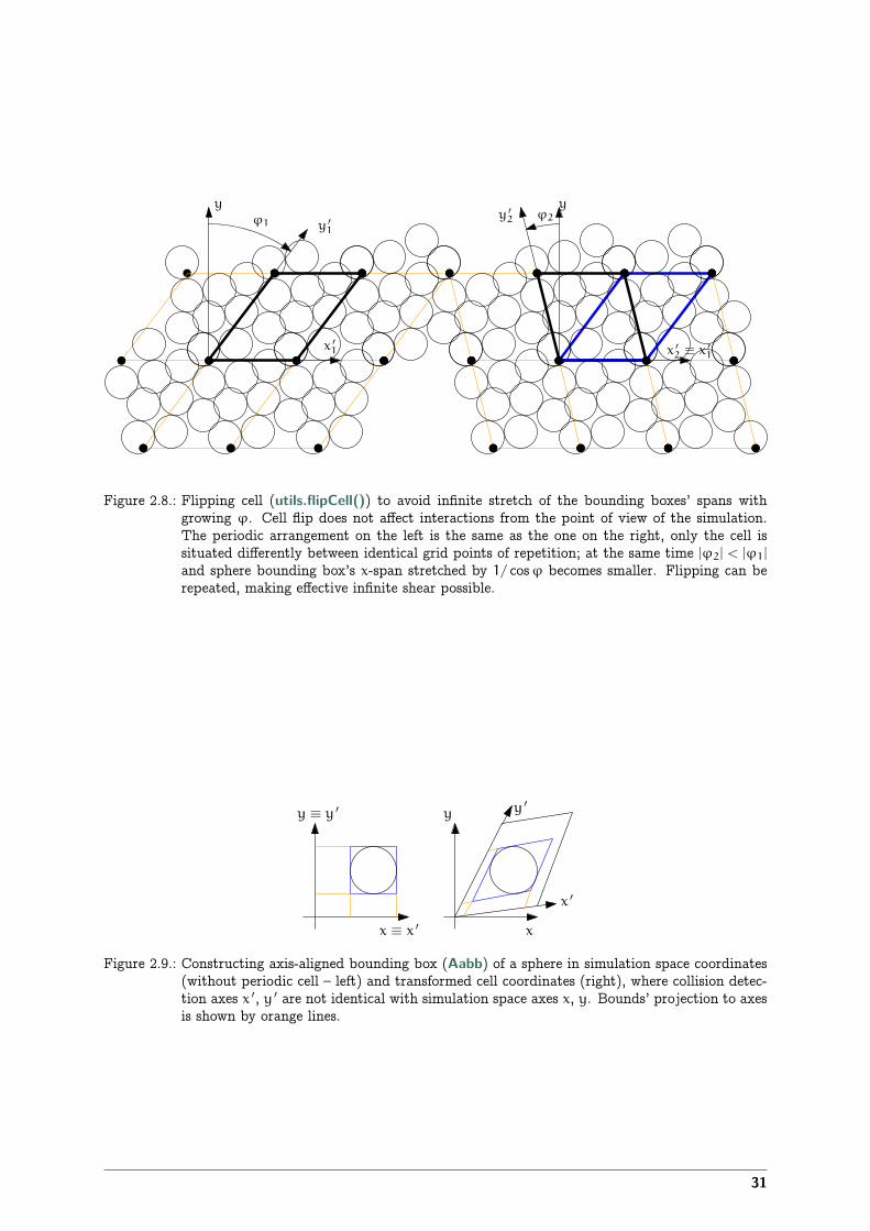
y ′1

y ′2

x ′1 x ′

2 ≡ x ′1

ϕ1

y yϕ2

Figure 2.8.: Flipping cell (utils.flipCell()) to avoid infinite stretch of the bounding boxes’ spans withgrowing φ. Cell flip does not affect interactions from the point of view of the simulation.The periodic arrangement on the left is the same as the one on the right, only the cell issituated differently between identical grid points of repetition; at the same time |φ2| < |φ1|

and sphere bounding box’s x-span stretched by 1/ cosφ becomes smaller. Flipping can berepeated, making effective infinite shear possible.

y ≡ y ′ y y ′

x ≡ x ′ x

x ′

Figure 2.9.: Constructing axis-aligned bounding box (Aabb) of a sphere in simulation space coordinates(without periodic cell – left) and transformed cell coordinates (right), where collision detec-tion axes x ′, y ′ are not identical with simulation space axes x, y. Bounds’ projection to axesis shown by orange lines.

31

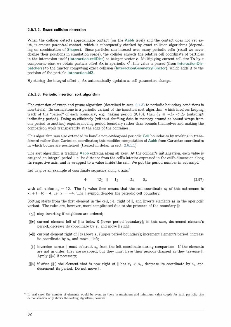
2.6.1.2. Exact collision detection

When the collider detects approximate contact (on the Aabb level) and the contact does not yet ex-ist, it creates potential contact, which is subsequently checked by exact collision algorithms (depend-ing on combination of Shapes). Since particles can interact over many periodic cells (recall we neverchange their positions in simulation space), the collider embeds the relative cell coordinate of particlesin the interaction itself (Interaction.cellDist) as integer vector c. Multiplying current cell size Ts by c

component-wise, we obtain particle offset ∆x in aperiodic R3; this value is passed (from InteractionDis-patchers) to the functor computing exact collision (InteractionGeometryFunctor), which adds it to theposition of the particle Interaction.id2.

By storing the integral offset c, ∆x automatically updates as cell parameters change.

2.6.1.3. Periodic insertion sort algorithm

The extension of sweep and prune algorithm (described in sect. 2.1.3) to periodic boundary conditions isnon-trivial. Its cornerstone is a periodic variant of the insertion sort algorithm, which involves keepingtrack of the “period” of each boundary; e.g. taking period ⟨0, 10), then 81 ≡ −22 < 22 (subscriptindicating period). Doing so efficiently (without shuffling data in memory around as bound wraps fromone period to another) requires moving period boundary rather than bounds themselves and making thecomparison work transparently at the edge of the container.

This algorithm was also extended to handle non-orthogonal periodic Cell boundaries by working in trans-formed rather than Cartesian coordinates; this modifies computation of Aabb from Cartesian coordinatesin which bodies are positioned (treated in detail in sect. 2.6.1.1).

The sort algorithm is tracking Aabb extrema along all axes. At the collider’s initialization, each value isassigned an integral period, i.e. its distance from the cell’s interior expressed in the cell’s dimension alongits respective axis, and is wrapped to a value inside the cell. We put the period number in subscript.

Let us give an example of coordinate sequence along x axis:6

41 122 || −12 −24 50 (2.97)

with cell x-size sx = 10. The 41 value then means that the real coordinate xi of this extremum isxi + 1 · 10 = 4, i.e. xi = −4. The || symbol denotes the periodic cell boundary.

Sorting starts from the first element in the cell, i.e. right of ||, and inverts elements as in the aperiodicvariant. The rules are, however, more complicated due to the presence of the boundary ||:

(≤) stop inverting if neighbors are ordered;

(||•) current element left of || is below 0 (lower period boundary); in this case, decrement element’speriod, decrease its coordinate by sx and move || right;

(•||) current element right of || is above sx (upper period boundary); increment element’s period, increaseits coordinate by sx and move || left;

(||<) inversion across || must subtract sx from the left coordinate during comparison. If the elementsare not in order, they are swapped, but they must have their periods changed as they traverse ||.Apply (||◦) if necessary;

(||◦) if after (||<) the element that is now right of || has xi < sx, decrease its coordinate by sx anddecrement its period. Do not move ||.

6 In real case, the number of elements would be even, as there is maximum and minimum value couple for each particle; thisdemonstration only shows the sorting algorithm, however.

32

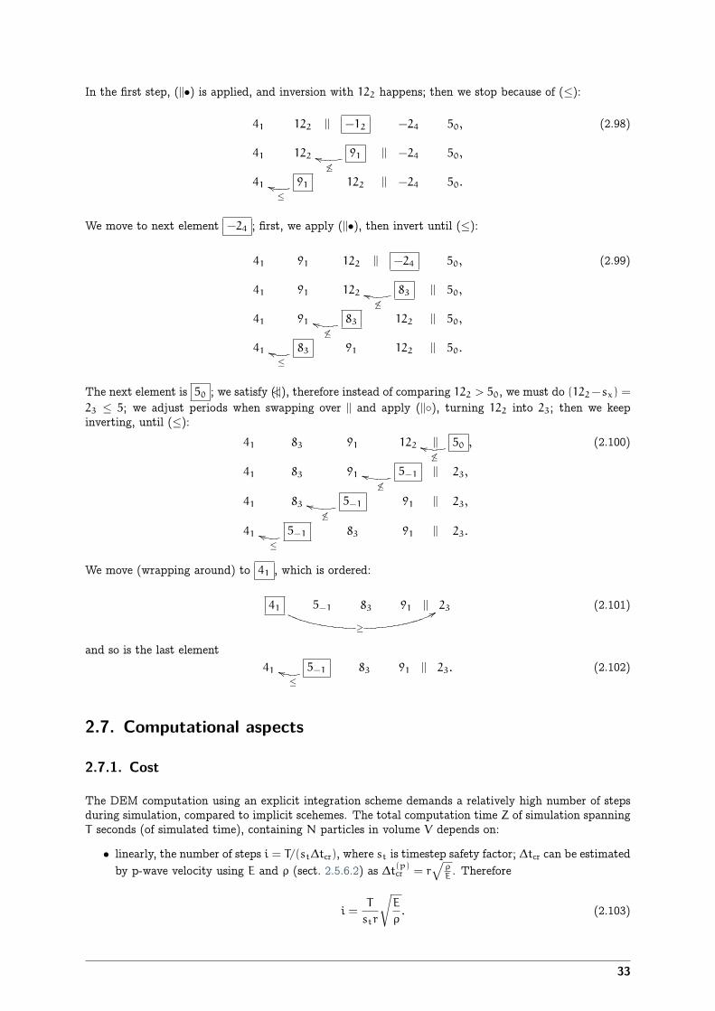
In the first step, (||•) is applied, and inversion with 122 happens; then we stop because of (≤):

41 122 || −12 −24 50,

41 122 91≤

jj || −24 50,

41 91≤

ii 122 || −24 50.

(2.98)

We move to next element −24 ; first, we apply (||•), then invert until (≤):

41 91 122 || −24 50,

41 91 122 83≤

jj || 50,

41 91 83≤

ii 122 || 50,

41 83≤

ii 91 122 || 50.

(2.99)

The next element is 50 ; we satisfy (||<), therefore instead of comparing 122 > 50, we must do (122−sx) =

23 ≤ 5; we adjust periods when swapping over || and apply (||◦), turning 122 into 23; then we keepinverting, until (≤):

41 83 91 122 || 50 ,≤

jj

41 83 91 5−1

≤jj || 23,

41 83 5−1

≤jj 91 || 23,

41 5−1

≤ii 83 91 || 23.

(2.100)

We move (wrapping around) to 41 , which is ordered:

41

≥

885−1 83 91 || 23 (2.101)

and so is the last element41 5−1

≤ii 83 91 || 23. (2.102)

2.7. Computational aspects

2.7.1. Cost

The DEM computation using an explicit integration scheme demands a relatively high number of stepsduring simulation, compared to implicit scehemes. The total computation time Z of simulation spanningT seconds (of simulated time), containing N particles in volume V depends on:

• linearly, the number of steps i = T/(st∆tcr), where st is timestep safety factor; ∆tcr can be estimatedby p-wave velocity using E and ρ (sect. 2.5.6.2) as ∆t(p)cr = r

»ρE. Therefore

i =T

str

 E

ρ. (2.103)

33

• the number of particles N; for fixed value of simulated domain volume V and particle radius r

N = pV

43πr3

, (2.104)

where p is packing porosity, roughly 12for dense irregular packings of spheres of similar radius.

The dependency is not strictly linear (which would be the best case), as some algorithms do notscale linearly; a case in point is the sweep and prune collision detection algorithm introduced insect. 2.1.3, with scaling roughly O(N logN).

The number of interactions scales with N, as long as packing characteristics are the same.

• the number of computational cores ncpu; in the ideal case, the dependency would be inverse-linearwere all algorithms parallelized (in Yade, collision detection is not).

Let us suppose linear scaling. Additionally, let us suppose that the material to be simulated (E, ρ) andthe simulation setup (V , T) are given in advance. Finally, dimensionless constants st, p and ncpu willhave a fixed value. This leaves us with one last degree of freedom, r. We may write

Z ∝ iN1

ncpu=

T

str

 E

ρp

V43πr3

1

ncpu∝ 1

r

1

r3=

1

r4. (2.105)

This (rather trivial) result is essential to realize DEM scaling; if we want to have finer results, refiningthe “mesh” by halving r, the computation time will grow 24 = 16 times.

For very crude estimates, one can use a known simulation to obtain a machine “constant”

µ =Z

Ni(2.106)

with the meaning of time per particle and per timestep (in the order of 10−6 s for current machines).µ will be only useful if simulation characteristics are similar and non-linearities in scaling do not havemajor influence, i.e. N should be in the same order of magnitude as in the reference case.

2.7.2. Result indeterminism

It is naturally expected that running the same simulation several times will give exactly the same results:although the computation is done with finite precision, round-off errors would be deterministically thesame at every run. While this is true for single-threaded computation where exact order of all operationsis given by the simulation itself, it is not true anymore in multi-threaded computation which is describedin detail in later sections.

The straight-forward manner of parallel processing in explicit DEM is given by the possibility of treatinginteractions in arbitrary order. Strain and stress is evaluated for each interaction independently, butforces from interactions have to be summed up. If summation order is also arbitrary (in Yade, forces areaccumulated for each thread in the order interactions are processed, then summed together), then theresults can be slightly different. For instance

(1/10.)+(1/13.)+(1/17.)=0.23574660633484162(1/17.)+(1/13.)+(1/10.)=0.23574660633484165

As forces generated by interactions are assigned to bodies in quasi-random order, summary force Fi onthe body can be different between single-threaded and multi-threaded computations, but also betweendifferent runs of multi-threaded computation with exactly the same parameters. Exact thread schedulingby the kernel is not predictable since it depends on asynchronous events (hardware interrupts) and otherunrelated tasks running on the system; and it is thread scheduling that ultimately determines summationorder of force contributions from interactions.

34

2.7.2.1. Numerical damping influence

The effect of summation order can be significantly amplified by the usage of a discontinuous dampingfunction in NewtonIntegrator given in (2.76) as

(∆F)dwFw

= −λd sgn FwÅu⊖w +

u◦w∆t

2

ã. (2.107)

If the sgn argument is close to zero then the least significant finite precision artifact can determine whetherthe equation (relative increment of Fw) is +λd or −λd. Given commonly used values of λd = 0.4, itmeans that such artifact propagates from least significant place to the most significant one at once.

35

3. Concrete particle model

This chapter presents a new model of concrete formulated within the DEM framework presented inchapter 2.

Contact law is formulated on the level of individual contacts between 2 particles. However, since de-sired results are macroscopic and not observed until larger simulations are performed, motivations forintroducing various contact-level features of the model might not be obvious until after reading sect. 3.3dedicated to calibration.

3.1. Discrete concrete models overview

Before describing the CPM model, we would like to give a brief overview of some of the main particle-based, DEM and non-DEM, concrete models.

Lattice models. Vervuurt [66, pg. 14–16] gives an overview of older lattice models used for con-crete. Later lattice models of concrete aim usually at meso-scale modeling, where aggregates and mortarare distinguished by differing beam parameters. Beam configuration can be regular (leading to failureanisotropy), random [35], or generated to match observed statistical distribution [33].

Lilliu and van Mier [35] uses brittle beam behavior, simply removing broken beams from simulation;Leite et al. [33] uses tensile softening to avoid dependence of global softening (which is observed evenwith brittle behavior of beams) on beam size. Neither of these models focuses on capturing compressionbehavior.

Cusatis et al. [9] presents a rather sophisticated model, in which properties of lattice beams are computedfrom the geometry of Voronoï cells of each node. Granulometry is supposed to have substantial influenceon confinement behavior; as it is not fully considered by the model, the beam-transversal stress historyinfluences shear rigidity instead. Compression behavior is captured fairly well.

Rigid body – spring models are, to our knowledge, used infrequently for concrete. Nagai et al. [41]presents a mesoscopic (distinguishing aggregates and mortar) model, though only formulated in 2D.

Discrete element models of concrete are rather rare. Most activity (judging by publications) comesfrom teams formed around Frédéric V. Donzé. His work (using SDEC software mentioned in sect. 4.1)first targeted at 2D DEM[5]. Later, exploiting the dynamic nature of DEM led to fast concrete dynamicsin 3D [19, 20] and impact simulation [59]. In order to reduce computational costs, elastic FEM for thenon-damaged subdomain is used, with some tricks to avoid spurious dynamic effects on the DEM/FEMboundary [54].

With both lattice and DEM models, arriving at reasonable compression behavior is non-trivial; it seemsto stem from the fact that 1D elements (beams in lattice, bonds in DEM) have no notion of an overallstress state at their vicinity, but only insofar as it is manifested in the direction of the respective element.Cusatis et al. [9] works around this by explicitly introducing the influence of transversal stress. Hentz [19,sect. 5.3], on the other hand, blocks rotations of spherical elements to achieve a higher and more realisticfc/ft ratio, but it is questionable whether there is physically sound reason for such an adjustment.

37

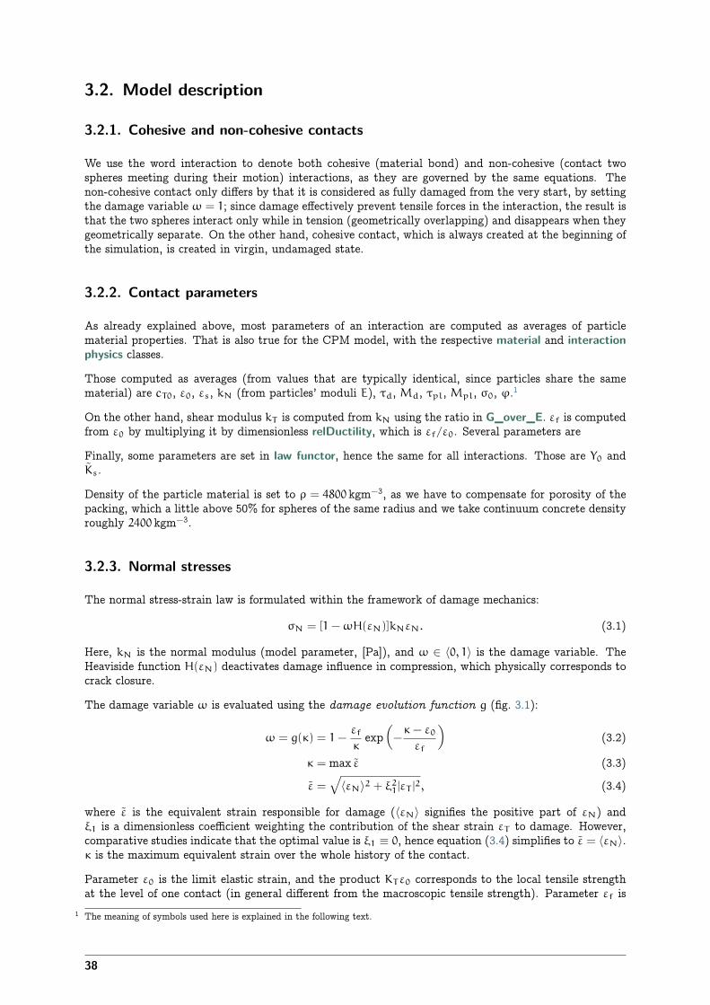
3.2. Model description

3.2.1. Cohesive and non-cohesive contacts

We use the word interaction to denote both cohesive (material bond) and non-cohesive (contact twospheres meeting during their motion) interactions, as they are governed by the same equations. Thenon-cohesive contact only differs by that it is considered as fully damaged from the very start, by settingthe damage variable ω = 1; since damage effectively prevent tensile forces in the interaction, the result isthat the two spheres interact only while in tension (geometrically overlapping) and disappears when theygeometrically separate. On the other hand, cohesive contact, which is always created at the beginning ofthe simulation, is created in virgin, undamaged state.

3.2.2. Contact parameters

As already explained above, most parameters of an interaction are computed as averages of particlematerial properties. That is also true for the CPM model, with the respective material and interactionphysics classes.

Those computed as averages (from values that are typically identical, since particles share the samematerial) are cT0, ε0, εs, kN (from particles’ moduli E), τd, Md, τpl, Mpl, σ0, φ.1

On the other hand, shear modulus kT is computed from kN using the ratio in G_over_E. εf is computedfrom ε0 by multiplying it by dimensionless relDuctility, which is εf/ε0. Several parameters are

Finally, some parameters are set in law functor, hence the same for all interactions. Those are Y0 andKs.

Density of the particle material is set to ρ = 4800 kgm−3, as we have to compensate for porosity of thepacking, which a little above 50% for spheres of the same radius and we take continuum concrete densityroughly 2400 kgm−3.

3.2.3. Normal stresses

The normal stress-strain law is formulated within the framework of damage mechanics:

σN = [1−ωH(εN)]kNεN. (3.1)

Here, kN is the normal modulus (model parameter, [Pa]), and ω ∈ ⟨0, 1⟩ is the damage variable. TheHeaviside function H(εN) deactivates damage influence in compression, which physically corresponds tocrack closure.

The damage variable ω is evaluated using the damage evolution function g (fig. 3.1):

ω = g(κ) = 1−εf

κexpÅ−κ− ε0

εf

ã(3.2)

κ = max ε (3.3)

ε =»⟨εN⟩2 + ξ21|εT |

2, (3.4)

where ε is the equivalent strain responsible for damage (⟨εN⟩ signifies the positive part of εN) andξ1 is a dimensionless coefficient weighting the contribution of the shear strain εT to damage. However,comparative studies indicate that the optimal value is ξ1 ≡ 0, hence equation (3.4) simplifies to ε = ⟨εN⟩.κ is the maximum equivalent strain over the whole history of the contact.

Parameter ε0 is the limit elastic strain, and the product KTε0 corresponds to the local tensile strengthat the level of one contact (in general different from the macroscopic tensile strength). Parameter εf is

1 The meaning of symbols used here is explained in the following text.

38

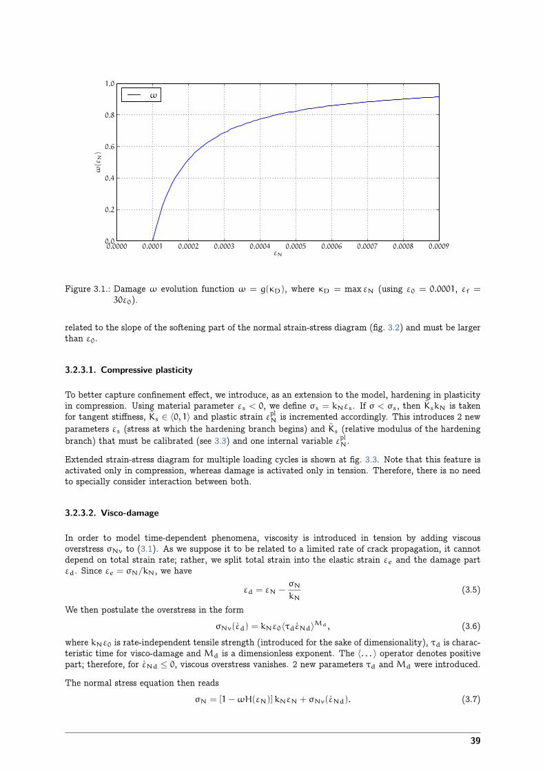
0.0000 0.0001 0.0002 0.0003 0.0004 0.0005 0.0006 0.0007 0.0008 0.0009εN

0.0

0.2

0.4

0.6

0.8

1.0

ω(εN

)ω

Figure 3.1.: Damage ω evolution function ω = g(κD), where κD = max εN (using ε0 = 0.0001, εf =30ε0).

related to the slope of the softening part of the normal strain-stress diagram (fig. 3.2) and must be largerthan ε0.

3.2.3.1. Compressive plasticity

To better capture confinement effect, we introduce, as an extension to the model, hardening in plasticityin compression. Using material parameter εs < 0, we define σs = kNεs. If σ < σs, then KskN is takenfor tangent stiffness, Ks ∈ ⟨0, 1⟩ and plastic strain ε

plN is incremented accordingly. This introduces 2 new

parameters εs (stress at which the hardening branch begins) and Ks (relative modulus of the hardeningbranch) that must be calibrated (see 3.3) and one internal variable ε

plN.

Extended strain-stress diagram for multiple loading cycles is shown at fig. 3.3. Note that this feature isactivated only in compression, whereas damage is activated only in tension. Therefore, there is no needto specially consider interaction between both.

3.2.3.2. Visco-damage

In order to model time-dependent phenomena, viscosity is introduced in tension by adding viscousoverstress σNv to (3.1). As we suppose it to be related to a limited rate of crack propagation, it cannotdepend on total strain rate; rather, we split total strain into the elastic strain εe and the damage partεd. Since εe = σN/kN, we have

εd = εN −σN

kN(3.5)

We then postulate the overstress in the formσNv(εd) = kNε0⟨τdεNd⟩Md , (3.6)

where kNε0 is rate-independent tensile strength (introduced for the sake of dimensionality), τd is charac-teristic time for visco-damage and Md is a dimensionless exponent. The ⟨. . . ⟩ operator denotes positivepart; therefore, for εNd ≤ 0, viscous overstress vanishes. 2 new parameters τd and Md were introduced.

The normal stress equation then readsσN = [1−ωH(εN)]kNεN + σNv(εNd). (3.7)

39

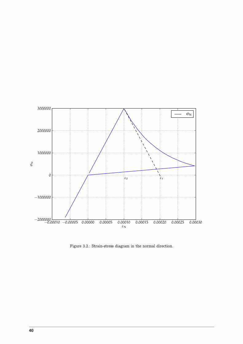
−0.00010 −0.00005 0.00000 0.00005 0.00010 0.00015 0.00020 0.00025 0.00030εN

−2000000

−1000000

0

1000000

2000000

3000000

σN

ε0 εf

σN

Figure 3.2.: Strain-stress diagram in the normal direction.

40

−0.0015 −0.0010 −0.0005 0.0000 0.0005 0.0010 0.0015 0.0020εN

−2.5

−2.0

−1.5

−1.0

−0.5

0.0

0.5

σN

×107

εs

σN

Figure 3.3.: Strain-stress diagram in normal direction, loaded cyclically in tension and compression; itshows several features of the model: (1) damage in tension, but not damage in compression(governed by the ω internal variable) (2) plasticity in compression, starting at strain εs;reduced (hardening) modulus is KskN.

41

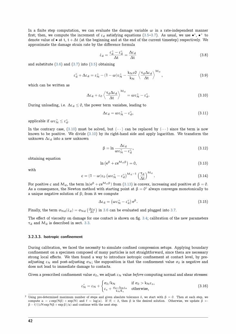
In a finite step computation, we can evaluate the damage variable ω in a rate-independent mannerfirst; then, we compute the increment of εd satisfying equations (3.5–3.7). As usual, we use •◦, •+ todenote value of • at t, t+∆t (at the beginning and at the end of the current timestep) respectively. Weapproximate the damage strain rate by the difference formula

εd =ε+d − ε◦d

∆t=

∆εd

∆t(3.8)

and substitute (3.6) and (3.7) into (3.5) obtaining

ε◦d + ∆εd = ε+N − (1−ω)ε+N −kNε0

kN

≠τd∆εd

∆t

∑Md

, (3.9)

which can be written as

∆εd + ε0

≠τd∆εd

∆t

∑Md

= ωε+N − ε◦d. (3.10)

During unloading, i.e. ∆εd ≤ 0, the power term vanishes, leading to

∆εd = ωε+N − ε◦d, (3.11)

applicable if ωε+N ≤ ε◦d.

In the contrary case, (3.10) must be solved, but ⟨· · · ⟩ can be replaced by (· · · ) since the term is nowknown to be positive. We divide (3.10) by its right-hand side and apply logarithm. We transform theunknown ∆εd into a new unknown

β = ln ∆εd

ωε+N − ε◦d, (3.12)

obtaining equationln

(eβ + ceMdβ

)= 0, (3.13)

withc = (1−ω)ε0

(ωε+N − ε◦d

)Md−1(τd∆t

)Md

. (3.14)

For positive c and Md, the term ln(eβ + ceMdβ) from (3.13) is convex, increasing and positive at β = 0.As a consequence, the Newton method with starting point at β = 02 always converges monotonically toa unique negative solution of β; from it we compute

∆εd =(ωε+N − ε◦d

)eβ. (3.15)

Finally, the term σNd(εd) = σNd

(∆εd

∆t

)in 3.6 can be evaluated and plugged into 3.7.

The effect of viscosity on damage for one contact is shown on fig. 3.4; calibration of the new parametersτd and Md is described in sect. 3.3.

3.2.3.3. Isotropic confinement

During calibration, we faced the necessity to simulate confined compression setups. Applying boundaryconfinement on a specimen composed of many particles is not straightforward, since thera are necessarystrong local effects. We then found a way to introduce isotropic confinement at contact level, by pre-adjusting εN and post-adjusting σN; the supposition is that the confinement value σ0 is negative anddoes not lead to immediate damage to contacts.

Given a prescribed confinement value σ0, we adjust εN value before computing normal and shear stresses:

ε ′N = εN +

{σ0/kN if σ0 > kNεs,εs +

σ0−kNεs

kNKsotherwise, (3.16)

2 Using pre-determined maximum number of steps and given absolute tolerance δ, we start with β = 0. Then at each step, wecompute a = c exp(Nβ) + exp(N) and f = log(a). If |f| < δ, then β is the desired solution. Otherwise, we update β ←β − f/((cN expNβ + expβ)/a) and continue with the next step.

42

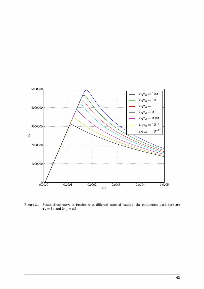
0.0000 0.0001 0.0002 0.0003 0.0004 0.0005εN

0

1000000

2000000

3000000

4000000

5000000

σN

εNτd = 100

εNτd = 10

εNτd = 1

εNτd = 0.1

εNτd = 0.001

εNτd = 10−6

εNτd = 10−12

Figure 3.4.: Strain-stress curve in tension with different rates of loading; the parameters used here areτd = 1 s and Md = 0.1.

43

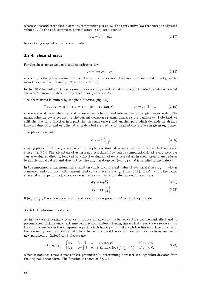
where the second case takes in account compressive plasticity. The constitutive law then uses the adjustedvalue ε ′

N. At the end, computed normal stress is adjusted back to

σ ′N = σN − σ0. (3.17)

before being applied on particle in contact.

3.2.4. Shear stresses

For the shear stress we use plastic constitutive law

σT = kT (εT − εTp) (3.18)

where εTp is the plastic strain on the contact and kT is shear contact modulus computed from kN as theratio kT/kN is fixed (usually 0.2, see the sect. 3.3).

In the DEM formulation (large strains), however, εTp is not stored and mapped contact points on elementsurfaces are moved instead as explained above, sect. 2.3.2.2.

The shear stress is limited by the yield function (fig. 3.5)

f(σN,σT ) = |σT |− rpl = |σT − (cT − σN tanφ), cT = cT0(1−ω) (3.19)

where material parameters cT0 and φ are initial cohesion and internal friction angle, respectively. Theinitial cohesion cT0 is reduced to the current cohesion cT using damage state variable ω. Note that wesplit the plasticity function in a part that depends on σT and another part which depends on alreadyknown values of ω and σN; the latter is denoted rpl, radius of the plasticity surface in given σN plane.

The plastic flow rule

εTp = λσT

|σT |, (3.20)

λ being plastic multiplier, is associated in the plane of shear stresses but not with respect to the normalstress (fig. 3.5). The advantage of using a non-associated flow rule is computational. At every step, σN

can be evaluated directly, followed by a direct evaluation of σT ; stress return in shear stress plane reducesto simple radial return and does not require any iterations as f(σN,σT ) = 0 is satisfied immediately.

In the implementation, numerical evaluation starts from current value of εT . Trial stress σtT = εTkT is

computed and compared with current plasticity surface radius rpl from (3.19). If |σtT | > rpl, the radial

stress return is performed; since we do not store εTp, εT is updated as well in such case:

σT = rpl”σT (3.21)

ε ′T = εT

|σT |

|σtT |

(3.22)

If |σtT | ≤ rpl, there is no plastic slip and we simply assign σT = σt

T without εT update.

3.2.4.1. Confinement extension

As in the case of normal stress, we introduce an extension to better capture confinement effect and toprevent shear locking under extreme compression: instead of using linear plastic surface we replace it bylogarithmic surface in the compression part, which has C1 continuity with the linear surface in tension;the continuity condition avoids pathologic behavior around the switch point and also reduces number ofnew parameters. Instead of (3.19), we use

f(σN, σT ) =

{|σT |− (cT0(1−ω) − σN tanφ) if σN ≥ 0

|σT |− cT0î(1−ω) + Y0 tanφ log

Ä−σN

cT0Y0+ 1äó

if σN < 0,(3.23)

which introduces a new dimensionless parameter Y0 determining how fast the logarithm deviates fromthe original, linear form. The function is shown at fig. 3.6.

44

cT0

σN

±|σT |

σT1

σT2

ϕrpl

Figure 3.5.: Linear yield surface and plastic flow rule.

−3.0 −2.5 −2.0 −1.5 −1.0 −0.5 0.0 0.5σN ×107

−3

−2

−1

0

1

2

3

±|σT|

×107

linear,ω=0linear,ω=1log+lin,ω=0log+lin,ω=1

Figure 3.6.: Comparison of linear and logarithmic (in compression) yield surfaces, for both virgin anddamaged material.

45

3.2.4.2. Visco-plasticity

Viscosity in shear uses similar ideas as visco-damage from sect. 3.2.3.2; the value of rt in (3.19) isaugmented depending on rate of plastic flow following the equation

r ′pl = rpl + cT0 (τplεTp)Mpl = rpl + cT0

Åτpl

∆εTp

∆t

ãMpl

(3.24)

where τpl is characteristic time for visco-plasticity, Mpl is a dimensionless exponent (both to be cali-brated. cT0 is undamaged cohesion introduced for the sake of dimensionality.

Similar solution strategy as for visco-damage is used, with different substitutions

β = lnÇ|σt

T |− r ′pl

|σtT |− rpl

å, (3.25)

c = cT0(|σt

T |− rpl)Mpl−1

Åτpl

kT∆t

ãMpl

. (3.26)

The equation to solve is then formally the same as (3.13)

ln(eβ + ceMplβ

)= 0. (3.27)

After finding β using the Newton-Raphson method, trial stress σtT is scaled by the factor

r ′pl

|σtT |

= 1− eβÅ1−

rpl

|σtT |

ã(3.28)

to obtain the final shear stress value

σT =r ′pl

|σtT |σtT . (3.29)

3.2.5. Applying stresses on particles

Resulting stresses σN and and σT are computed at the current contact point C◦. Summary forceFΣ = Aeq(σNn+ σT ) has to be applied to particle’s positions C◦

1, C◦2, exerting force and torque:

F1 = FΣ, T1 = (C◦ −C◦1)× FΣ, (3.30)

F2 = −FΣ, T2 = −(C◦ −C◦1)× FΣ. (3.31)

Forces and torques on particles from multiple interactions accumulate during one computation step.

3.2.6. Contact model summary

The computation described above proceeds in the following order:

Isotropic confinement σ0 is applied if active. This consists in adjusting normal strain to either εN ←εN + σ0 (if σ0 ≥ kNεs) or εN ← εs + (σ0 − kNεs)/(kNKs).

Normal stress σN. ε = ⟨εN⟩ is computed, then the history variable is updated κ ← max(κ, ε); κ isthe state variable from which the current damage ω = g(k) = 1 − (εf/κ) exp(−(κ − ε0)/εf) isevaluated; for non-cohesive contacts, however, we set ω = 1. For cohesive contacts with damagedisabled (CpmPhys.neverDamage), we set ω = 0.

The state variable εplN (initially zero) holds the normal plastic strain; we use it to compute the

elastic part of the current strain εelN = εN − εplN.

Normal stress is computed using the equation of damage mechanics σN = (1−H(εelN)ω)kNεelN.

46

Whether compressive hardening is present is determined; σNs = kN(εs + Ks(εN − εs)) is pre-evaluated; then if εelN < εs and σNs > σN, normal stress and normal plastic strains are updatedεplN ← ε

plN +(σN −σNs)/kN, σN ← σNs. If the condition is not satisfied, compressive plasticity has

no effect and does not have to be specifically considered.

Shear stress σT . First, trial value is computed simply from σT ← kTεT . This value will be com-pared with the radius of plastic surface rpl for given, already known σN. As there are differ-ent plasticity functions for tension and compression, we obtain rpl = cT0(1 − ω) − σN tanφ forσN ≥ 0; in compression, the logarithmic surface makes the formula more complicated, givingrpl = cT0 [(1−ω) + Y0 tanφ(−σN/(cT0Y0) + 1)].

If the trial stress is beyond the admissible range, i.e. |σT | > rpl, plastic flow will take place. Sincethe total formulation for strain is used, we update the εT to have the same direction, but themagnitude of |σT |/kT .

Without visco-plasticity (the default), a simple update σT ← (σT/|σT |)rpl is performed duringthe plastic flow. If visco-plasticity is used, we update σT ← sσT , s being a scaling scalar. It iscomputed as s = 1−eβ(1−rpl/|σT |), where β is solved with Newton-Raphson iteration as describedabove, with the coefficient c = cT0(τpl/(kT∆t))

Mpl(|σT |− rpl)Mpl−1 and the exponent Mpl.

Viscous normal overstress σNv is applied for cohesive contacts only. As explained above, it is effectivefor non-zero damage rate. When damage is not growing (i.e. the state variable εd ≥ εNω, whereεd is initially zero), we simply update εd ← εNω, and the overstress is zero

Otherwise, the viscosity equation has to be solved using the coefficient c = ε0(1 −ω)(τd/∆t)

Md(εNω − εd)Md−1 and the exponent N = Md; once β is solved with the Newton-

Raphson method as shown above, we update εd ← εd + (εNω − εd)eβ and finally obtain

σNv = (εNω− εd)kN. Then the overstress is applied via σN ← σN + σNv.

3.3. Parameter calibration

The model comprises two sets of parameters that determine elastic and inelastic behavior. In order tomatch simulations to experiments, a procedure to calibrate these parameters must be given. Since elasticproperties are independent of inelastic ones, they are calibrated first.

Model parameters can be summarized as follows:

1. geometry

r sphere radiusRI interaction radius

2. elasticity

kN normal contact stiffnesskT/kN relative shear contact stiffness

3. damage and plasticity

ε0 limit elastic strainεf parameter of damage evolution function

CT0 shear cohesion of undamaged materialφ internal friction angle

4. confinement

Y0 parameter for plastic surface evolution in compressionεs hardening strain in compressionKs relative hardening modulus in compression

47

5. rate-dependence

τd characteristic time for visco-damageMd dimensionless visco-damage exponentτpl characteristic time for visco-plasticity

Mpl dimensionless visco-plasticity exponent

Macroscopic properties should be matched to prescribed values by running simulation on sufficientlylarge specimen. Let us give overview of them, in the order of calibration:

1. elastic properties, which depend on only geometry and elastic parameters (using grouping from thelist above)

E Young’s modulus,ν Poisson’s ratio

2. inelastic properties, depending (in addition) on damage and plasticity parameters:

ft tensile strengthfc compressive strengthGf fracture energy (conventional definition shown in fig. 3.7)

3. confinement properties; they appear only in high confinement situations and can be calibratedwithout having substantial impact on already calibrated inelastic properties. We do not describethem quantitatively; fitting simulation and experimental curves is used instead.

4. rate-dependence properties; they appear only in high-rate situations, therefore are again calibratedafter inelastic properties independently. As in the previous case, a simple fitting approach is usedhere.

3.3.1. Simulation setup

In order to calibrate macroscopic properties, simulations with multiple particles have to be run. Thisallows to smooth away different orientation of individual contacts and gives apparent continuum-likebehavior.

We were running simple strain-controlled tension/compression (UniaxialStrainer) test on a 1:1:2 cuboid-shaped specimen of 2000 spheres.3 Straining is applied in the direction of the longest dimension, onboundary particles; they are identified, on the “positive” and “negative” end of the specimen, by distancefrom bounding box of the specimen; as result, roughly one layer of spheres is considered as support on eachside. Distance between (some) two spheres on each end along the strained axis determines the referencelength l0; specimen elongation is computed from their current distance divided by l0 during subsequentsimulation. Straining imposes displacement on support particles along strained axis, symmetrically oneither end of the specimen (half on the “positive” and half on the “negative” boundary particles), while alltheir other degrees of freedom are kept free, including perpendicular translations, leading to simulationof frictionless supports.

Axial force F is computed by averaging sums of forces on support particles from both supports F+ and−F−. Divided by specimen cross-section A, average stress is obtained. The cross-section area is estimatedas either cross-section of the specimen’s bounding box (for cuboid specimen) or as minimum of severalareas Ai of convex hull around particles intersecting perpendicular plane at different coordinates alongthe axis (for non-prismatic specimen) – see fig. 3.8.

Such tension/compression test can be found in the examples/concrete/uniax.py script.

Periodic boundary conditions were not implemented in Yade until later stages of the thesis (the Cellclass). In such case, determining deformation and cross-section area is much simpler, as it exists ob-

3 Later, the test was being done on hyperboloid-shaped specimen, to pre-determine fracturing area, while avoiding boundary effects.

48

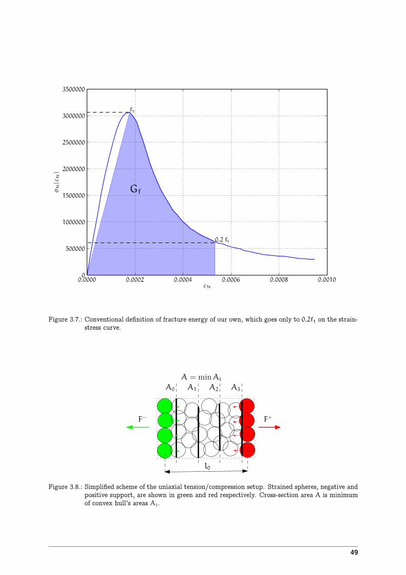
0.0000 0.0002 0.0004 0.0006 0.0008 0.0010εN

0

500000

1000000

1500000

2000000

2500000

3000000

3500000

σN

(εN

)

ft

0.2 ft

Gf

Figure 3.7.: Conventional definition of fracture energy of our own, which goes only to 0.2ft on the strain-stress curve.

l0

F− F+

A0 A1 A2 A3

A = minAi

Figure 3.8.: Simplified scheme of the uniaxial tension/compression setup. Strained spheres, negative andpositive support, are shown in green and red respectively. Cross-section area A is minimumof convex hull’s areas Ai.

49

jectively, embodies in the periodic cell size. Computing stress is equally trivial: first, vector of sumof all forces on interactions in the cell (taking tensile forces as positive and compressive as negative) iscomputed, then divided by-component by perpendicular areas of the cell. This is handled by PeriTriax-Compressor and PeriTriaxController classes.

3.3.1.1. Stress tensor evaluation in arbitrary volume

Computation of stress from reaction forces is not suitable for cases where the loading scenario is not asstraight-forwardly defined as in the case of uniaxial tension/compression. For general case, an equationfor stress tensor can be derived. Using the work of Kuhl et al. [31], eqs. (33) and (35), we have

σ =1

V

∑c∈V

[FcΣ ⊗ (C2 −C1)]sym

= (3.32)

=1

V

∑c∈V

lcîNcFcN + TcTFcT

ó(3.33)

where V is the considered volume containing interactions with the c index. For each interaction, there isl = |C2 −C1|, FΣ = FNn+ FT , with all variables assuming their current value. We use 2nd-order normalprojection tensor N = n⊗ n which, evaluated component-wise, gives

Nij = ninj. (3.34)

The 3rd-order tangential projection tensor TT = Isym · n− n⊗ n⊗ n is written by components

TTijk =

1

2(δikδjl + δilδjk)nl − ninjnk = (3.35)

=δiknj

2+

δjkni

2− ninjnk. (3.36)

Plugging these expressions into (3.33) gives

σij =∑c∈V

ncin

cj F

cN +

ncj F

cTi

2+

nciF

cTj

2− nc

incj n

ckF

cTk︸ ︷︷ ︸

= 0, since nc ⊥ FcT

(3.37)

Results from this formula were slightly lower than stress obtained from support reaction forces. It islikely due to small number of interaction in V; we were considering an interaction inside if the contactpoint was inside spherical V , which can also happen for an interaction between two spheres outside V ;some weighting function could be used to avoid V boundary problems.

Boundary effect is avoided for periodic cell (Cell), where the volume V is defined by its size and allinteraction would are summed together.

This algorithm is implemented in the eudoxos.InteractionLocator.macroAroundPt() method.

3.3.2. Geometry and elastic parameters

Let us recall the parameters that influence the elastic response of the model:

Radius r. The radius is considered to be the same for all the spheres, for the following two reasons:

1. The time step of the computation (which is one of the main factors determining computationalcosts) depends on the smallest critical time step for all bodies. Small elements have a smallercritical time step, therefore they would negatively impact the performance.

2. A direct correlation of macroscopic and contact-level properties is based on the assumptionthat the sphere radii are the same.

50

Interaction radius RI is the relative distance determining the „non-locality“ of contact detection. ForRI = 1, only spheres that touch are considered as being in contact. In general, the condition reads

d0 ≤ RI(r1 + r2). (3.38)

The value of RI directly influences the average number of interactions per sphere (percolation).For our purposes, we recommend to use RI = 1.5, which gives the average of ≈12 interactions persphere for packing with density > 0.5.

This value was determined experimentally based on the average number of interactions; it stabilizesthe packing with regards to contact-level phenomena (damage) and makes the model, in a way,“non-local”.

RI also importantly influences the ft/fc ratio, which was the original motivation for increasing itsvalue from 1.

RI only serves to create initial (cohesive) interactions in the packing; after the initial step, inter-actions having been established, it is reset to 1. A disadvantage is that fractured material whichbecomes compact again (such as dust compaction) will have a smaller elastic stiffness, since it willhave a smaller number of contacts per sphere.

kN and kT are contact moduli in the normal and shear directions introduced above.

These 4 parameters should be calibrated in such way that the given macroscopic properties E and ν arematched. It can be shown by dimensional analysis that ν depends on the dimensionless ratio kN/kT and,if RI is fixed, Young’s modulus is proportional to kN (at fixed kN/kT ).

By analogy with the microplane theory, the dependence can be derived analytically (see [31]) as

ν =kN − kT

4kN + kT=

1− kT/kN

4+ kT/kN, (3.39)

which matches quite well the results our simulations (fig. 3.9). Stránský et al. [63] reports similarnumerical results, which get closer to theoretical values as RI grows.

For E, similar equations can be derived, leading to

E

kN=

∑AiLi

3V

2+ 3 kT

kN

4+ kT

kN

, (3.40)

where Ai is cross-sectional area of contact number i, Li is its length and V is the volume of space in whichthe spheres are placed (total volume of the given sample). The first fraction, volume ratio, is determinedsolely by the interaction radius RI; therefore, E depends linearly on KN.

In our case, however, we simply run elastic simulation to determine the actual E/kN ratio (3.40). Toobtain desired macroscopic modulus of E∗, the value of kN is scaled by E∗/E.

3.3.2.1. Measuring macroscopic elastic properties

Measuring linear properties in dynamic simulations faces 2 sources of non-linearity:

1. Dynamic oscillations may influence results if strain rate is too high. This can be avoided bystopping loading at some point and letting kinetic energy dissipate by using numerical damping(NewtonIntegrator.damping).

2. Early non-linear behavior might disturb the results. For avoiding damage, special flag Cpm-Mat.neverDamage was introduced to the material, causing it to never damage. To prevent plas-ticity, loading to low strains is necessary. However, due to RI = 1.5, there will be no plasticbehavior (rearranging particles under initial load, which would make the response artificially morecompliant) until later loading stages.

51

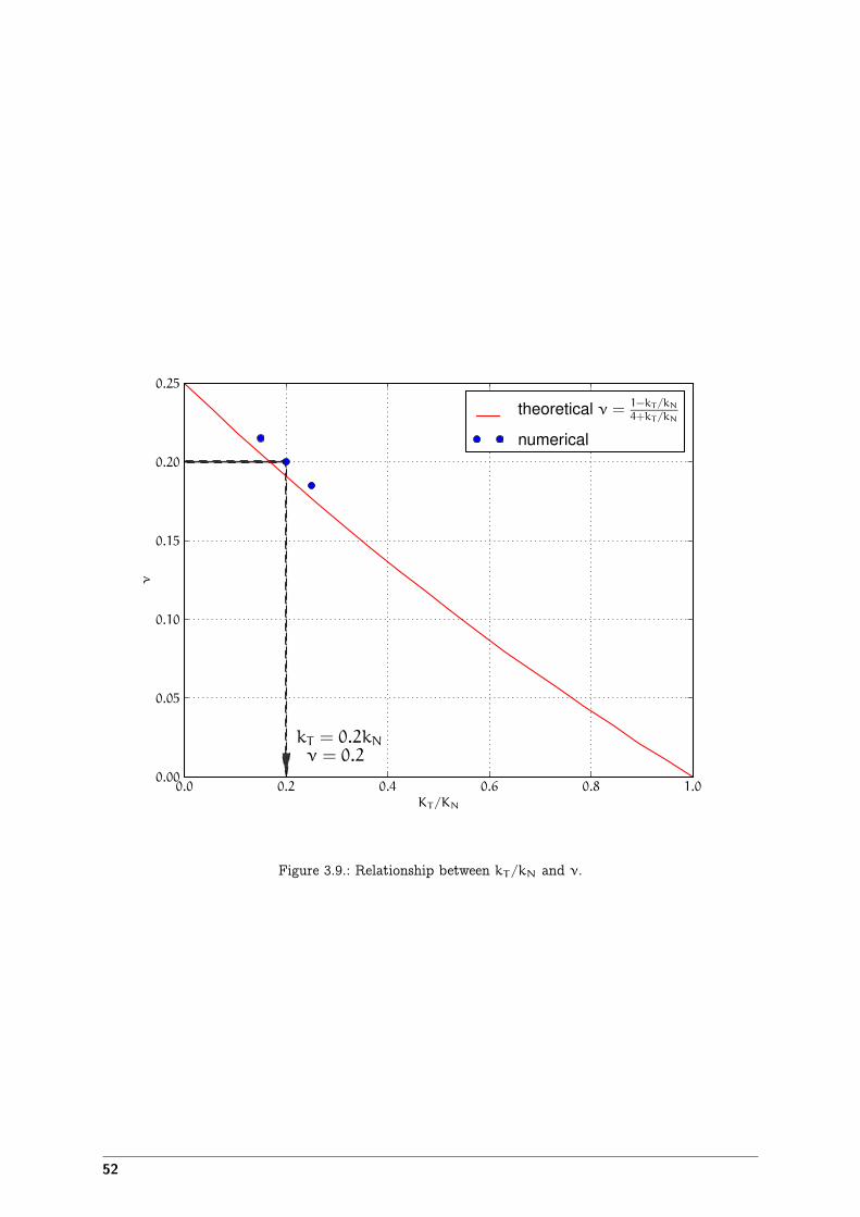
0.0 0.2 0.4 0.6 0.8 1.0KT/KN

0.00

0.05

0.10

0.15

0.20

0.25

ν

kT = 0.2kNν = 0.2

theoretical ν = 1−kT/kN4+kT/kN

numerical

Figure 3.9.: Relationship between kT/kN and ν.

52

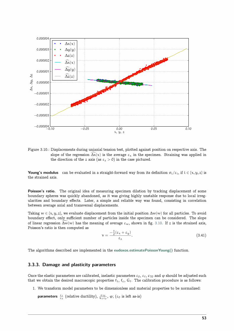
−0.10 −0.05 0.00 0.05 0.10x, y, z

−0.000004

−0.000003

−0.000002

−0.000001

0.000000

0.000001

0.000002

0.000003

0.000004

∆x,∆y,∆z

∆x(x)

∆y(y)

∆z(z)

∆x(x)

∆y(y)

∆z(z)

Figure 3.10.: Displacements during uniaxial tension test, plotted against position on respective axis. Theslope of the regression ”∆x(x) is the average εx in the specimen. Straining was applied inthe direction of the z axis (as εz > 0) in the case pictured.

Young’s modulus can be evaluated in a straight-forward way from its definition σi/εi, if i ∈ {x, y, z} isthe strained axis.

Poisson’s ratio. The original idea of measuring specimen dilation by tracking displacement of someboundary spheres was quickly abandoned, as it was giving highly unstable response due to local irreg-ularities and boundary effects. Later, a simple and reliable way was found, consisting in correlationbetween average axial and transversal displacements.

Taking w ∈ {x, y, z}, we evaluate displacement from the initial position ∆w(w) for all particles. To avoidboundary effect, only sufficient number of particles inside the specimen can be considered. The slopeof linear regression ∆w(w) has the meaning of average εw, shown in fig. 3.10. If z is the strained axis,Poisson’s ratio is then computed as

ν =−1

2(εx + εy)

εz. (3.41)

The algorithms described are implemented in the eudoxos.estimatePoissonYoung() function.

3.3.3. Damage and plasticity parameters

Once the elastic parameters are calibrated, inelastic parameters ε0, εf, cT0 and φ should be adjusted suchthat we obtain the desired macroscopic properties ft, fc, Gf. The calibration procedure is as follows:

1. We transform model parameters to be dimensionless and material properties to be normalized:

parameters εf

ε0(relative ductility), cT0

kTε0, φ; (ε0 is left as-is)

53

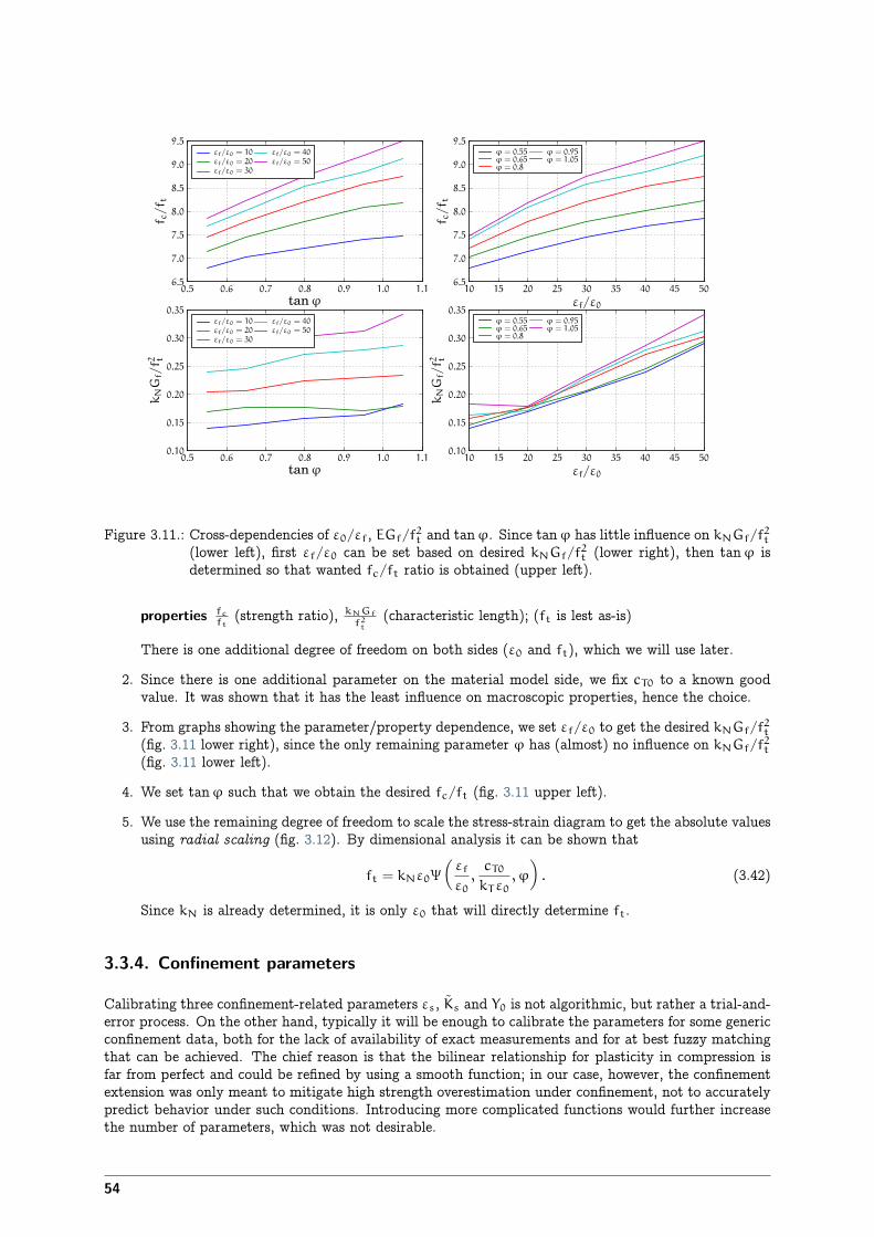
0.5 0.6 0.7 0.8 0.9 1.0 1.1

tanϕ6.5

7.0

7.5

8.0

8.5

9.0

9.5

f c/f t

εf/ε0 = 10εf/ε0 = 20εf/ε0 = 30

εf/ε0 = 40εf/ε0 = 50

0.5 0.6 0.7 0.8 0.9 1.0 1.1

tanϕ0.10

0.15

0.20

0.25

0.30

0.35

kNGf/f2 t

εf/ε0 = 10εf/ε0 = 20εf/ε0 = 30

εf/ε0 = 40εf/ε0 = 50

10 15 20 25 30 35 40 45 50

εf/ε0

6.5

7.0

7.5

8.0

8.5

9.0

9.5

f c/f t

ϕ = 0.55ϕ = 0.65ϕ = 0.8

ϕ = 0.95ϕ = 1.05

10 15 20 25 30 35 40 45 50

εf/ε0

0.10

0.15

0.20

0.25

0.30

0.35

kNGf/f2 t

ϕ = 0.55ϕ = 0.65ϕ = 0.8

ϕ = 0.95ϕ = 1.05

Figure 3.11.: Cross-dependencies of ε0/εf, EGf/f2t and tanφ. Since tanφ has little influence on kNGf/f

2t

(lower left), first εf/ε0 can be set based on desired kNGf/f2t (lower right), then tanφ is

determined so that wanted fc/ft ratio is obtained (upper left).

properties fcft

(strength ratio), kNGf

f2t

(characteristic length); (ft is lest as-is)

There is one additional degree of freedom on both sides (ε0 and ft), which we will use later.

2. Since there is one additional parameter on the material model side, we fix cT0 to a known goodvalue. It was shown that it has the least influence on macroscopic properties, hence the choice.

3. From graphs showing the parameter/property dependence, we set εf/ε0 to get the desired kNGf/f2t

(fig. 3.11 lower right), since the only remaining parameter φ has (almost) no influence on kNGf/f2t

(fig. 3.11 lower left).

4. We set tanφ such that we obtain the desired fc/ft (fig. 3.11 upper left).

5. We use the remaining degree of freedom to scale the stress-strain diagram to get the absolute valuesusing radial scaling (fig. 3.12). By dimensional analysis it can be shown that

ft = kNε0Ψ

Åεf

ε0,cT0

kTε0, φ

ã. (3.42)

Since kN is already determined, it is only ε0 that will directly determine ft.

3.3.4. Confinement parameters

Calibrating three confinement-related parameters εs, Ks and Y0 is not algorithmic, but rather a trial-and-error process. On the other hand, typically it will be enough to calibrate the parameters for some genericconfinement data, both for the lack of availability of exact measurements and for at best fuzzy matchingthat can be achieved. The chief reason is that the bilinear relationship for plasticity in compression isfar from perfect and could be refined by using a smooth function; in our case, however, the confinementextension was only meant to mitigate high strength overestimation under confinement, not to accuratelypredict behavior under such conditions. Introducing more complicated functions would further increasethe number of parameters, which was not desirable.

54

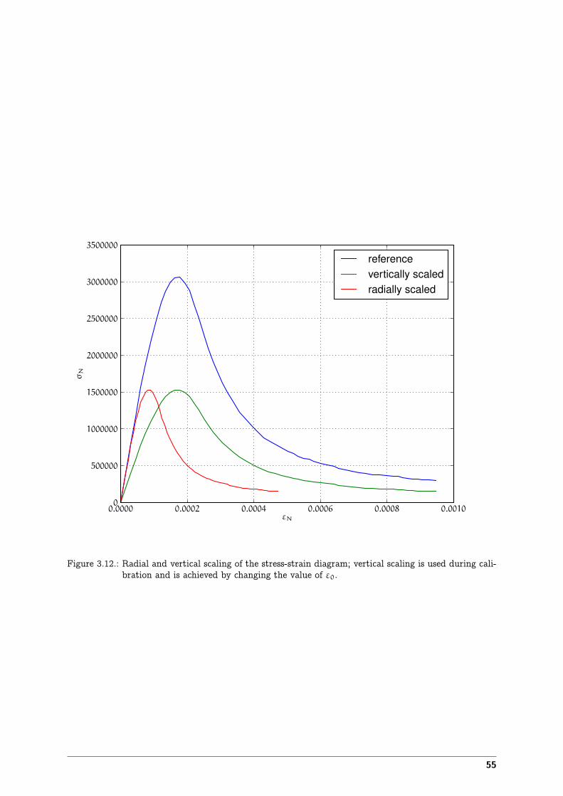
0.0000 0.0002 0.0004 0.0006 0.0008 0.0010εN

0

500000

1000000

1500000

2000000

2500000

3000000

3500000

σN

referencevertically scaledradially scaled

Figure 3.12.: Radial and vertical scaling of the stress-strain diagram; vertical scaling is used during cali-bration and is achieved by changing the value of ε0.

55

−0.05 −0.04 −0.03 −0.02 −0.01 0.00εN

−1.4

−1.2

−1.0

−0.8

−0.6

−0.4

−0.2

0.0σN

[Pa]

×109exp 20 MPanum 20 MPaexp 100 MPanum 100 MPaexp 200 MPanum 200 MPaexp 400 MPanum 400 MPa

Figure 3.13.: Confined compression, comparing experimental data and simulation without the confine-ment extensions of the model. Experimental results (dashed) from Caner and Bažant [6].

The experimental data we use come from [6] and [16].

Consider confined strain-stress diagrams at fig. 3.13 exhibiting unrealistic behavior under high confine-ment (-400MPa). Parameters εs and Ks will influence at which point the curve will get to the hardeningbranch and what will be its tangent modulus (fig. 3.3). The Y0 parameter determines evolution ofplasticity surface in compression (fig 3.6). We recommend the following values of the parameters:

εs = −3 · 10−3, Ks = 0.3, Y0 = 0.1, (3.43)

which give curves in fig. 3.14. It was observed when running multiple simulations that results underhigh confinement depend greatly on the exact packing configuration, specimen shape and specimen size;therefore, the values given above should be taken with grain of salt.

During simulation, the confinement effect was introduced on the contact level, in the constitutive lawitself, as described in sect. 3.2.3.3; the confinement is therefore isotropic and without boundary influence.

Cross-dependencies. Confinement properties may, to certain extent, have influence on inelastic prop-erties. If that happens, reiterating the calibration with new confinement properties should give wantedresults quickly.

3.3.5. Rate-dependence parameters

The visco-damage behavior in tension introduced two parameters, characteristic time τd and exponentMd. There is no calibration procedure developed for them, as measuring the response is experimentally

56

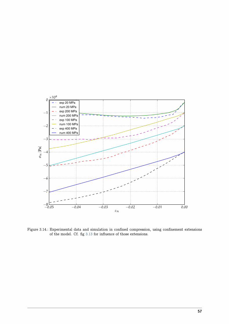
−0.05 −0.04 −0.03 −0.02 −0.01 0.00εN

−8

−7

−6

−5

−4

−3

−2

−1

0

σN

[Pa]

×108exp 20 MPanum 20 MPaexp 200 MPanum 200 MPaexp 100 MPanum 100 MPaexp 400 MPanum 400 MPa

Figure 3.14.: Experimental data and simulation in confined compression, using confinement extensionsof the model. Cf. fig 3.13 for influence of those extensions.

57

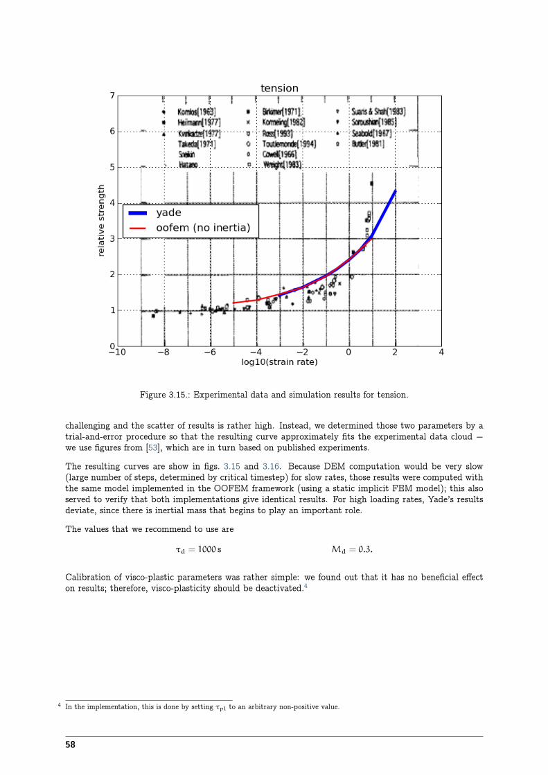
Figure 3.15.: Experimental data and simulation results for tension.

challenging and the scatter of results is rather high. Instead, we determined those two parameters by atrial-and-error procedure so that the resulting curve approximately fits the experimental data cloud −we use figures from [53], which are in turn based on published experiments.

The resulting curves are show in figs. 3.15 and 3.16. Because DEM computation would be very slow(large number of steps, determined by critical timestep) for slow rates, those results were computed withthe same model implemented in the OOFEM framework (using a static implicit FEM model); this alsoserved to verify that both implementations give identical results. For high loading rates, Yade’s resultsdeviate, since there is inertial mass that begins to play an important role.

The values that we recommend to use are

τd = 1000 s Md = 0.3.

Calibration of visco-plastic parameters was rather simple: we found out that it has no beneficial effecton results; therefore, visco-plasticity should be deactivated.4

4 In the implementation, this is done by setting τpl to an arbitrary non-positive value.

58

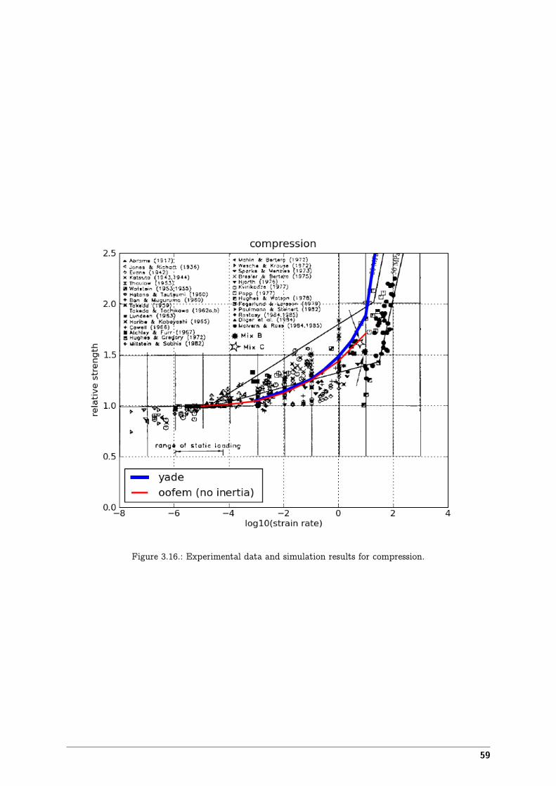
Figure 3.16.: Experimental data and simulation results for compression.

59

Part II.

The Yade platform

61

4. Overview

4.1. History

In 1990, Frédéric Donzé started “Spherical Discrete Element Code” (SDEC, Donzé [11]), using rigidspherical particles in 3d, with explicit leap-frog integration scheme, using elastic-brittle behavior in thenormal sense and Mohr-Coulomb criterion for shear.

Already in mid-1990s, SDEC inspired first version of ESyS-Particle [14], which was focusing on high-performance computing and was developed in-house at that time.

Having perceived inflexibility of SDEC in face of new emerging methods and method couplings, Donzéinitiated [71] conception of Yade, flexible platform for dynamic computing in 2004. The initial implemen-tation was done in c++ by Jan Kozicki and Olivier Galizzi, back-then both working at the University ofGrenoble. The platform was supposed to unite multiple different methods (FEM, DEM, lattice models,mass-spring models, realtime rigidbody dynamics), but with the exception of DEM and lattice models,they all stagnated at proof-of-concept stage.

Many advanced programming concepts were used (polymorphism, multiple dispatch, plugins); the origi-nal framework was described in (belated) papers Kozicki and Donzé [29, 30].

Arguably, the framework was over-designed with much more framework than functionality, poorly doc-umented; that was criticised by the author of this paper [67]. In years 2007–2010, I became the the defacto lead developer and Yade underwent several significant changes:

Python scripting interface using boost::python was the most important and involved change and war-rants its dedicated section 4.2.4.

Code cleanup, removing unused, incomplete or poorly functioning classes. Most classes were renamedfor consistency, and many abstraction layers were removed. This made Yade perhaps less flexible,but more functional.

Documentation within the source code, setting up wiki.

Community moving development resources to launchpad.net, animating mailing lists, initiating dedi-cated website https://www.yade-dem.org. The community currently counts (based on list sub-scription counts) 60 users and 27 developers.

Parallel computation on shared-memory multiprocessors, using relatively non-intrusive OpenMP frame-work. This makes the computation (roughly) 5.5 × faster on 8 cores. Lots of other performance-related improvements were done as well.

4.2. Software architecture

The original Yade design was described in Kozicki and Donzé [29]; although some parts are alreadyrefactored, it still contains useful overview of patters that gave rise to Yade. The current architecture isdescribed, from programmer’s point of view, in the Programmer’s manual, chapter 7.

The framework has layered structure; any part can only depend on a same-level or a lower-level part:

63

Libraries is the lowest level defining functionality which is not related specifically to simulations; thisentails mathematics (vector, quaternion, simple matrix algebra), serialization (storing arbitraryclass instances to file and restoring them later), multimethods (described below), OpenGL-relatedfunctions for 3d display, import functions for foreign file formats (STereo Litography), etc.

External libraries also count to this layer. Yade tries to delegate as much as possible to other(high-quality) open-source codes; in particular, various boost.org libraries are used extensively.

Core layer defines the most abstract simulation-related classes, such as Scene, Body (particle), Inter-action, Engine. It contains the executable as well (which is itself in python) and could be run,though uselessly, without higher levels.

Common layer defines data structures useful for different simulation methods, not only DEM, such asspherical particle, elastic material, approximate collision detection, generic OpenGL renderer.

Specialized layer contains functionality for particular simulation methods. This layer used to containDEM, FEM, lattice, basic realtime-rigidbody, … implementations; at this moment, only DEM isused, making the distinction between “common” and “specialized” layers less obvious than it wasoriginally planned.

The framework is implemented in c++ and is trying to use many features c++ offers, where it makessense; readers not familiar with them can find introductory paragraphs in Appendix A.

4.2.1. Documentation

As is the case with many research programs, documentation was severely lacking [67]. Although Doxygencomments were in place, they were unpractical due to

1. Heavy use of templates, creating many unreadable symbols,

2. Length of generation and size of documentation files (of which chief part was occupied by PNGimages of call graphs for each class)

3. Lack of integration with python, of which need didn’t emerge until python started to be usedseriously.

Sphinx was chosen as the tool for documenting python code (since Python 2.5, it is the documentationtool for Python itself as well, see http://docs.python.org/). Documentation for c++ classes andtheir attributes is put in special preprocessor macros; as most c++ classes are mirrored in Pythonautomatically, this documentation becomes docstring of that object in python, allowing effectively tocreate documentation for the c++ class by documenting the wrapper class in python. Sphinx allows fairlycomplicated markup (math, images, lists, footnotes, citations) and, most importantly, easily integratesautomatically-generated documentation with hand-written, continuous text. Finally, Sphinx handlesmultiple output formats; its LATEX output made it possible to include large parts of Yade documentation(available online at https://www.yade-dem.org/sphinx/) directly in this thesis.

Although the documentation is still far from being complete, it is already useful for newcomers as wellas moderately experienced users.

4.2.2. Modularity

The original modularity idea was that users will locally compile their own classes, independent of thosealready distributed. In practice, this has never been the case, as the code was not stable and bug-free enough to make the separation of core and external plugins meaningful. Despite that, plugins areconveniently used to conditionally disable parts of functionality, quickly change only part of code withoutrecompiling the rest and so on. Plugin functionality is composed of several otherwise-unrelated features:

1. Plugin can be queried what classes they provide, when being loaded.

64

2. Classes can be instantiated based on their name. Classes are not binary objects as e.g. functionsare (of which pointer can be retrieved via a dlsym(. . . ) call); therefore, factory function, whichreturns pointer to new instance every time called, must be defined for each class.

A special object, usually called class factory, keeps track of all factory functions; given an identifier ofclass (which is usually its name as string), it finds associated factory function, calls it and returns pointerto the new instance. User is then responsible to cast this pointer from generic type1 to appropriate specialtype.

4.2.3. Serialization

Serialization refers to converting arbitrary in-memory object to is serial representation, from which itcan be reconstructed again (deserialization). All objects that are able to serialize themselves derivefrom Serializable class and can enumerate attributes describing their state which must be serialized;those attributes must be again serializable: either a Serializable, or primitive serializable type (number,vector, string, etc).

Since the whole simulation (Scene class) is a Serializable, it can be saved to file (using fairly readableXML representation) and reloaded later.

Currently, Yade uses its own serialization framework. Using (much faster) boost::serialization instead isalready possible with special compile-time switches and will be preferred in the future.

4.2.4. Python interface

Scripting languages in general provide fast, easy and flexible way to control numerical programs [32].Python was the language of choice for Yade, used for simulation setup (which proved to be the mostfuture-compatible format), control, debug-inspection and post-processing.

Integration of Python into Yade evolved in several (unplanned) steps over years:

1. Primitive and explicit wrapping of a few basic functions controlling the simulation.

2. Explicit wrapping of base classes which was abusing serialization interface for attribute access(hence all attributes had to be converted to string first, then back). Derived classes were onlyinstantiated using special syntax.

3. Explicit wrapping of base classes, but providing native implementations of attribute access viamacros; instantiation of derived classes was handled via proxy metaclasses constructed from Yade’sinternal RTTI information.

4. Implicit wrapping of all classes, using macros in class declarations, including native attribute ac-cess, documentation, and proper type hierarchy reflected in python; class objects are injected intodedicated namespace by special virtual functions called when plugin class is being registered atstartup.

Shared pointers,2 which are used for memory management throughout Yade, integrate seamlesslywith boost::python, as they are used automatically to manage lifetime of wrapped objects, avoidingbig potential source of invalid memory accesses.

Plans for the future include seamless deriving of python classes from c++ classes including virtualfunction calls by using the special boost::python::wrapper class.

1 Generic pointer type can be void*, but also parent class of all factorable types; in Yade, such class is named Factorable andreturned pointers are of type shared ptr⟨Factorable⟩.

2 Shared pointers are provided by boost::shared_ptr and are already standardized in the updated C++09 standard, currentlyaccessible under namespace of Technical Report 1 (tr1::shared_ptr) on compilers that support it.

65

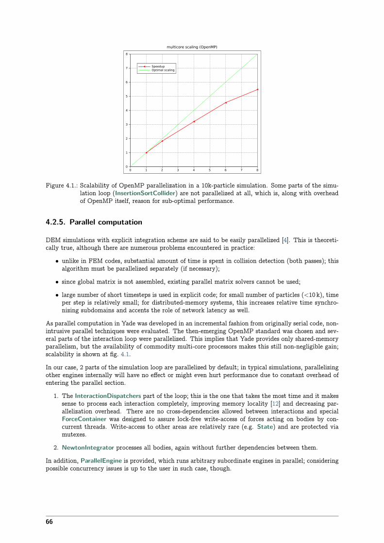
multicore scaling (OpenMP)

0 1 2 3 4 5 6 7 80

1

2

3

4

5

6

7

8

SpeedupOptimal scaling

Figure 4.1.: Scalability of OpenMP parallelization in a 10k-particle simulation. Some parts of the simu-lation loop (InsertionSortCollider) are not parallelized at all, which is, along with overheadof OpenMP itself, reason for sub-optimal performance.

4.2.5. Parallel computation

DEM simulations with explicit integration scheme are said to be easily parallelized [4]. This is theoreti-cally true, although there are numerous problems encountered in practice:

• unlike in FEM codes, substantial amount of time is spent in collision detection (both passes); thisalgorithm must be parallelized separately (if necessary);

• since global matrix is not assembled, existing parallel matrix solvers cannot be used;

• large number of short timesteps is used in explicit code; for small number of particles (<10 k), timeper step is relatively small; for distributed-memory systems, this increases relative time synchro-nizing subdomains and accents the role of network latency as well.

As parallel computation in Yade was developed in an incremental fashion from originally serial code, non-intrusive parallel techniques were evaluated. The then-emerging OpenMP standard was chosen and sev-eral parts of the interaction loop were parallelized. This implies that Yade provides only shared-memoryparallelism, but the availability of commodity multi-core processors makes this still non-negligible gain;scalability is shown at fig. 4.1.

In our case, 2 parts of the simulation loop are parallelized by default; in typical simulations, parallelizingother engines internally will have no effect or might even hurt performance due to constant overhead ofentering the parallel section.

1. The InteractionDispatchers part of the loop; this is the one that takes the most time and it makessense to process each interaction completely, improving memory locality [12] and decreasing par-allelization overhead. There are no cross-dependencies allowed between interactions and specialForceContainer was designed to assure lock-free write-access of forces acting on bodies by con-current threads. Write-access to other areas are relatively rare (e.g. State) and are protected viamutexes.

2. NewtonIntegrator processes all bodies, again without further dependencies between them.

In addition, ParallelEngine is provided, which runs arbitrary subordinate engines in parallel; consideringpossible concurrency issues is up to the user in such case, though.

66

4.2.6. Dispatchers and functors

Frequently, dispatching to functors depending on exact argument types (generalization of virtual func-tions) is necessary; a typical example is handling collisions between different combinations of shapes:

InteractionGeometryDispatcher([Ig2_Sphere_Sphere_Dem3DofGeom(),Ig2_Facet_Sphere_Dem3DofGeom()

]),

The dispatcher will ask its functors for types they receive (Sphere+Sphere in the first case, Facet+Spherein the second). Number of types the dispatcher decides upon is arity of the functor; in our case, n = 2.Calling the dispatcher performs the following behind scenes:3

1. Determine types of all relevant (n) arguments; this is implemented using regular virtual functions,which returns class index statically associated with each class.

2. Lookup in n-dimensional dispatch matrix containing (shared) functor pointers. If successful, thefunctor is called, being passed appropriate arguments.

Direct lookup failure results in attempting dispatch for base classes of the argument’s types recur-sively; if successful, functor minimizing type distance4 is called; matrix entries are filled to returnthat functor for direct argument types next time immediately (caching).

If recursive lookup fails, exception is thrown.

Although this algorithm is relatively “fast” (2 virtual function calls, functor pointer dereference, functor’svirtual function call), the fact of it being performed several thousand times in each step (of which numberis typically in the order of 105) makes it sensible to improve it further.

Our implementation finally caches functor pointers inside simulation objects, making dispatch matrixlookup necessary only at the first call for each interaction. All further calls reduce to pointer dereferenceand functor (virtual) call.5

3 As noted in Appendix A, multivirtual functions are not part of the c++ standard. Even if it were the case, however, we want tobe able to provide different functors for resolving the call, which wouldn’t be (most likely) possible with regular multi-methods.

4 Sum of distances of argument type and type the functor accepts for all dimensions of the dispatch matrix.5 Because this is still not optimal, there are plans to move algorithms of functors into static functions; their (non-virtual) address

could be cached and called without any overhead then.

67

5. Introduction

5.1. Getting started

Before you start moving around in Yade, you should have some prior knowledge.

• Basics of command line in your Linux system are necessary for running yade. Look on the web fortutorials.

• Python language; we recommend the official Python tutorial. Reading further documents on thetopis, such as Dive into Python will certainly not hurt either.

You are advised to try all commands described yourself. Don’t be afraid to experiment.

5.1.1. Starting yade

Yade is being run primarily from terminal; the name of command is yade. 1 (In case you did not installfrom package, you might need to give specific path to the command 2 ):

$ yadeWelcome to Yade bzr1984TCP python prompt on localhost:9001, auth cookie `sdksuy'TCP info provider on localhost:21000[[ ^L clears screen, ^U kills line. F12 controller, F11 3d view, F10 both, F9 generator, F8 plot. ]]Yade [1]:

These initial lines give you some information about

• version (bzr1984); always state this version you use if you seek help in the community or reportbug;

• some information for Remote control, which you are unlikely to need now;

• basic help for the command-line that just appeared (Yade [1]:).

Type quit(), exit() or simply press ^D to quit Yade.

The command-line is ipython, python shell with enhanced interactive capabilities; it features persistent

1 The executable name can carry a suffix, such as version number (yade-0.20), depending on compilation options. Packaged versionson Debian systems always provide the plain yade alias, by default pointing to latest stable version (or latest snapshot, if no stableversion is installed). You can use update-alternatives to change this.

2 In general, Unix shell (command line) has environment variable PATH defined, which determines directories searched for executablefiles if you give name of the file without path. Typically, $PATH contains /usr/bin/, /usr/local/bin, /bin and others; you caninspect your PATH by typing echo $PATH in the shell (directories are separated by :).

If Yade executable is not in directory contained in PATH, you have to specify it by hand, i.e. by typing the path in front of thefilename, such as in /home/user/bin/yade and similar. You can also navigate to the directory itself (cd ~/bin/yade, where ~ isreplaced by your home directory automatically) and type ./yade then (the . is the current directory, so ./ specifies that the file isto be found in the current directory).

To save typing, you can add the directory where Yade is installed to your PATH, typically by editing ~/.profile (in normal casesautomatically executed when shell starts up) file adding line like export PATH=/home/user/bin:$PATH. You can also define analias by saying alias yade=”/home/users/bin/yade” in that file.

Details depend on what shell you use (bash, zsh, tcsh, …) and you will find more information in introductory material onLinux/Unix.

69

history (remembers commands from your last sessions), searching and so on. See ipython’s documentationfor more details.

Typically, you will not type Yade commands by hand, but use scripts, python programs describing andrunning your simulations. Let us take the most simple script that will just print “Hello world!”:print "Hello world!"

Saving such script as hello.py, it can be given as argument to yade:

$ yade script.pyWelcome to Yade bzr1986TCP python prompt on localhost:9001, auth cookie `askcsu'TCP info provider on localhost:21000Running script hello.py ## the script is being runHello world! ## output from the script[[ ^L clears screen, ^U kills line. F12 controller, F11 3d view, F10 both, F9 generator, F8 plot. ]]Yade [1]:

Yade will run the script and then drop to the command-line again. 3 If you want Yade to quit immediatelyafter running the script, use the -x switch:

$ yade -x script.py

There is more command-line options than just -x, run yade -h to see all of them.

5.1.2. Creating simulation

To create simulation, one can either use a specialized class of type FileGenerator to create full scene,possibly receiving some parameters. Generators are written in c++ and their role is limited to well-defined scenarios. For instance, to create triaxial test scene:

Yade [4]: TriaxialTest(numberOfGrains=200).load()

Yade [5]: len(O.bodies)-> [5]: 184

Generators are regular yade objects that support attribute access.

It is also possible to construct the scene by a python script; this gives much more flexibility and speed ofdevelopment and is the recommended way to create simulation. Yade provides modules for streamlinedbody construction, import of geometries from files and reuse of common code. Since this topic is moreinvolved, it is explained in the User’s manual.

5.1.3. Running simulation

As explained above, the loop consists in running defined sequence of engines. Step number can be queriedby O.iter and advancing by one step is done by O.step(). Every step advances virtual time by currenttimestep, O.dt:

Yade [7]: O.iter-> [7]: 0

Yade [8]: O.time-> [8]: 0.0

3 Plain Python interpreter exits once it finishes running the script. The reason why Yade does the contrary is that most of thetime script only sets up simulation and lets it run; since computation typically runs in background thread, the script is technicallyfinished, but the computation is running.

70

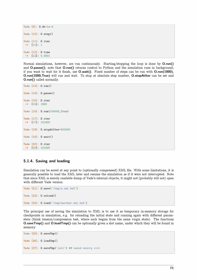
Yade [9]: O.dt=1e-4

Yade [10]: O.step()

Yade [11]: O.iter-> [11]: 1

Yade [12]: O.time-> [12]: 0.0001

Normal simulations, however, are run continuously. Starting/stopping the loop is done by O.run()and O.pause(); note that O.run() returns control to Python and the simulation runs in background;if you want to wait for it finish, use O.wait(). Fixed number of steps can be run with O.run(1000),O.run(1000,True) will run and wait. To stop at absolute step number, O.stopAtIter can be set andO.run() called normally.

Yade [13]: O.run()

Yade [14]: O.pause()

Yade [15]: O.iter-> [15]: 1920

Yade [16]: O.run(100000,True)

Yade [17]: O.iter-> [17]: 101920

Yade [18]: O.stopAtIter=500000

Yade [19]: O.wait()

Yade [20]: O.iter-> [20]: 101920

5.1.4. Saving and loading

Simulation can be saved at any point to (optionally compressed) XML file. With some limitations, it isgenerally possible to load the XML later and resume the simulation as if it were not interrupted. Notethat since XML is merely readable dump of Yade’s internal objects, it might not (probably will not) openwith different Yade version.

Yade [21]: O.save('/tmp/a.xml.bz2')

Yade [22]: O.reload()

Yade [24]: O.load('/tmp/another.xml.bz2')

The principal use of saving the simulation to XML is to use it as temporary in-memory storage forcheckpoints in simulation, e.g. for reloading the initial state and running again with different param-eters (think tension/compression test, where each begins from the same virgin state). The functionsO.saveTmp() and O.loadTmp() can be optionally given a slot name, under which they will be found inmemory:

Yade [25]: O.saveTmp()

Yade [26]: O.loadTmp()

Yade [27]: O.saveTmp('init') ## named memory slot

71

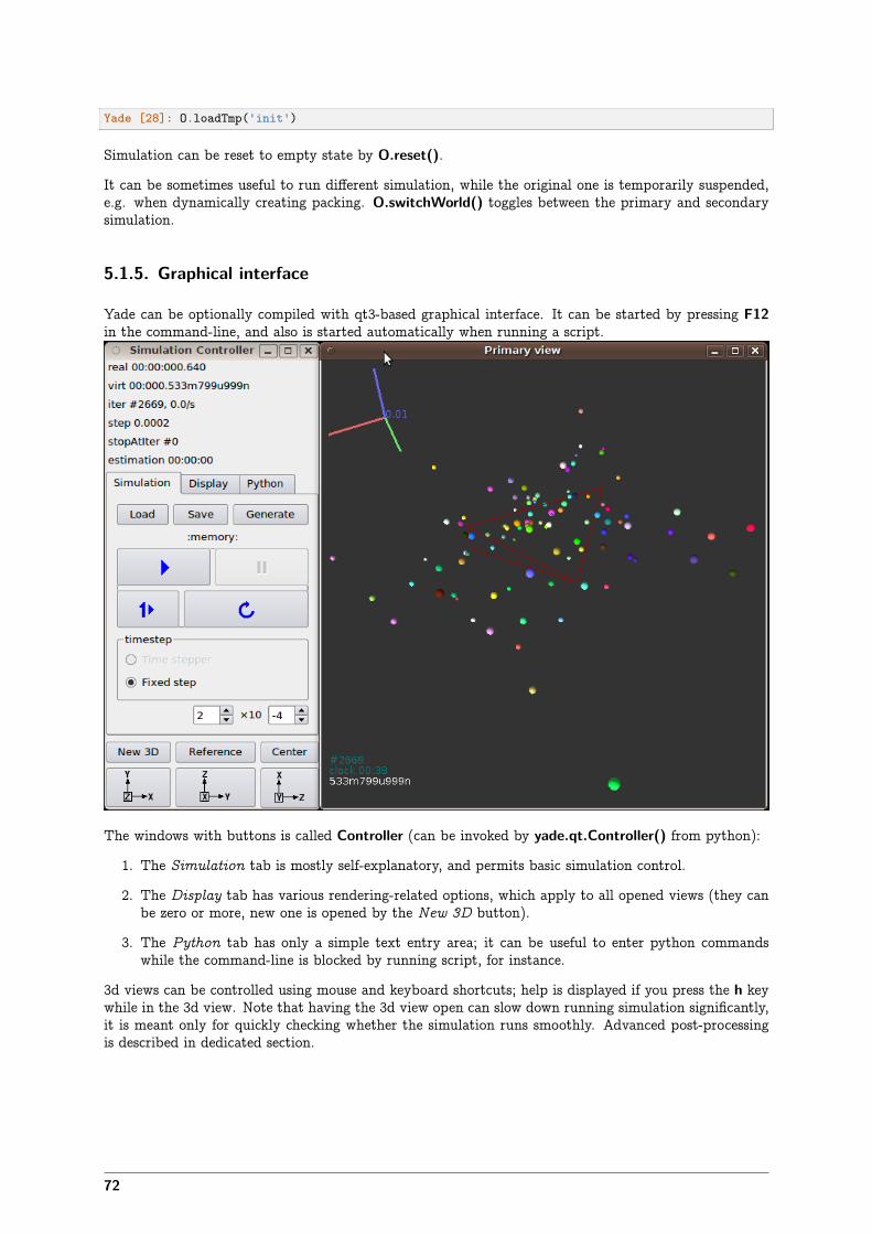
Yade [28]: O.loadTmp('init')

Simulation can be reset to empty state by O.reset().

It can be sometimes useful to run different simulation, while the original one is temporarily suspended,e.g. when dynamically creating packing. O.switchWorld() toggles between the primary and secondarysimulation.

5.1.5. Graphical interface

Yade can be optionally compiled with qt3-based graphical interface. It can be started by pressing F12in the command-line, and also is started automatically when running a script.

The windows with buttons is called Controller (can be invoked by yade.qt.Controller() from python):

1. The Simulation tab is mostly self-explanatory, and permits basic simulation control.

2. The Display tab has various rendering-related options, which apply to all opened views (they canbe zero or more, new one is opened by the New 3D button).

3. The Python tab has only a simple text entry area; it can be useful to enter python commandswhile the command-line is blocked by running script, for instance.

3d views can be controlled using mouse and keyboard shortcuts; help is displayed if you press the h keywhile in the 3d view. Note that having the 3d view open can slow down running simulation significantly,it is meant only for quickly checking whether the simulation runs smoothly. Advanced post-processingis described in dedicated section.

72

5.2. Architecture overview

In the following, a high-level overview of Yade architecture will be given. As many of the features aredirectly represented in simulation scripts, which are written in Python, being familiar with this languagewill help you follow the examples. For the rest, this knowledge is not strictly necessary and you canignore code examples.

5.2.1. Data and functions

To assure flexibility of software design, yade makes clear distinction of 2 families of classes: data com-ponents and functional components. The former only store data without providing functionality, whilethe latter define functions operating on the data. In programming, this is known as visitor pattern (asfunctional components “visit” the data, without being bound to them explicitly).

Entire simulation, i.e. both data and functions, are stored in a single Scene object. It is accessiblethrough the Omega class in python (a singleton), which is by default stored in the O global variable:

Yade [32]: O.bodies # some data components-> [32]: <yade.wrapper.BodyContainer object at 0x29ed320>

Yade [33]: len(O.bodies) # there are no bodies as of yet-> [33]: 0

Yade [34]: O.engines # functional components, empty at the moment-> [34]: []

5.2.1.1. Data components

Bodies Yade simulation (class Scene) is represented by Bodies, their Interactions and resultant gener-alized forces (all stored internally in special containers).

Each Body comprises the following:

Shape represents particle’s geometry (neutral with regards to its spatial orientation), such as Sphere,Facet or inifinite Wall; it usually does not change during simulation.

Material stores characteristics pertaining to mechanical behavior, such as Young’s modulus or density,which are independent on particle’s shape and dimensions; usually constant, might be sharedamongst multiple bodies.

State contains state variable variables, in particular spatial position and orientation, linear and angularvelocity, linear and angular accelerator; it is updated by the integrator at every step.

Derived classes can hold additional data, e.g. averaged damage.

Bound is used for approximate (“pass 1”) contact detection; updated as necessary following body’s mo-tion. Currently, Aabb is used most often as Bound. Some bodies may have no Bound, in whichcase they are exempt from contact detection.

(In addition to these 4 components, bodies have several more minor data associated, such as Body::id orBody::mask.)

All these four properties can be of different types, derived from their respective base types. Yade fre-quently makes decisions about computation based on those types: Sphere + Sphere collision has to betreated differently than Facet + Sphere collision. Objects making those decisions are called Dispatcher‘sand are essential to understand Yade’s functioning; they are discussed below.

Explicitly assigning all 4 properties to each particle by hand would be not practical; there are utilityfunctions defined to create them with all necessary ingredients. For example, we can create sphere particle

73

using utils.sphere:

Yade [35]: s=utils.sphere(center=[0,0,0],radius=1)

Yade [36]: s.shape, s.state, s.mat, s.bound-> [36]:(<Sphere instance at 0x2a8f030>,<State instance at 0x2eb4b90>,<FrictMat instance at 0x24500e0>,<Aabb instance at 0x2ce9590>)

Yade [37]: s.state.pos-> [37]: Vector3(0,0,0)

Yade [38]: s.shape.radius-> [38]: 1.0

We see that a sphere with material of type FrictMat (default, unless you provide another Material) andbounding volume of type Aabb (axis-aligned bounding box) was created. Its position is at origin and itsradius is 1.0. Finally, this object can be inserted into the simulation; and we can insert yet one sphereas well.

Yade [39]: O.bodies.append(s)-> [39]: 0

Yade [40]: O.bodies.append(utils.sphere([0,0,2],.5))-> [40]: 1

In each case, return value is Body.id of the body inserted.

Since till now the simulation was empty, its id is 0 for the first sphere and 1 for the second one. Saving theid value is not necessary, unless you want access this particular body later; it is remembered internallyin Body itself. You can address bodies by their id:

Yade [41]: O.bodies[1].state.pos-> [41]: Vector3(0,0,2)

Yade [42]: O.bodies[100]---------------------------------------------------------------------------IndexError Traceback (most recent call last)

/home/vaclav/ydoc/<ipython console> in <module>()

IndexError: Body id out of range.

Adding the same body twice is, for reasons of the id uniqueness, not allowed:

Yade [43]: O.bodies.append(s)---------------------------------------------------------------------------IndexError Traceback (most recent call last)

/home/vaclav/ydoc/<ipython console> in <module>()

IndexError: Body already has id 0 set; appending such body (for the second time) is not allowed.

Bodies can be iterated over using standard python iteration syntax:

Yade [44]: for b in O.bodies:....: print b.id,b.shape.radius....:

0 1.01 0.5

74

Interactions Interactions are always between pair of bodies; usually, they are created by the colliderbased on spatial proximity; they can, however, be created explicitly and exist independently of distance.Each interaction has 2 components:

InteractionGeometry holding geometrical configuration of the two particles in collision; it is updatedautomatically as the particles in question move and can be queried for various geometrical charac-teristics, such as penetration distance or shear strain.

Based on combination of types of Shapes of the particles, there might be different storage require-ments; for that reason, a number of derived classes exists, e.g. for representing geometry of contactbetween Sphere+Sphere, Facet+Sphere etc.

InteractionPhysics representing non-geometrical features of the interaction; some are computed fromMaterials of the particles in contact using some averaging algorithm (such as contact stiffness fromYoung’s moduli of particles), others might be internal variables like damage.

Suppose now interactions have been already created. We can access them by the id pair:Yade [48]: O.interactions[0,1]-> [48]: <Interaction instance at 0x267f4f0>

Yade [49]: O.interactions[1,0] # order of ids is not important-> [49]: <Interaction instance at 0x267f4f0>

Yade [50]: i=O.interactions[0,1]

Yade [51]: i.id1,i.id2-> [51]: (0, 1)

Yade [52]: i.geom-> [52]: <Dem3DofGeom_SphereSphere instance at 0x2f786b0>

Yade [53]: i.phys-> [53]: <FrictPhys instance at 0x2666f10>

Yade [54]: O.interactions[100,10111]---------------------------------------------------------------------------IndexError Traceback (most recent call last)

/home/vaclav/ydoc/<ipython console> in <module>()

IndexError: No such interaction

Generalized forces Generalized forces include force, torque and forced displacement and rotation; theyare stored only temporarliy, during one computation step, and reset to zero afterwards. For reasons ofparallel computation, they work as accumulators, i.e. only can be added to, read and reset.Yade [55]: O.forces.f(0)-> [55]: Vector3(0,0,0)

Yade [56]: O.forces.addF(0,Vector3(1,2,3))

Yade [57]: O.forces.f(0)-> [57]: Vector3(1,2,3)

You will only rarely modify forces from Python; it is usually done in c++ code and relevant documen-tation can be found in the Programmer’s manual.

5.2.1.2. Function components

In a typical DEM simulation, the following sequence is run repeatedly:

75

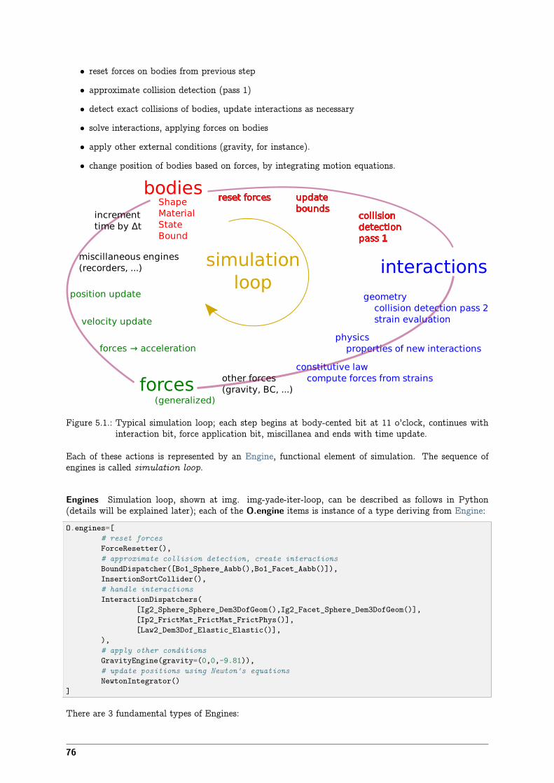
• reset forces on bodies from previous step

• approximate collision detection (pass 1)

• detect exact collisions of bodies, update interactions as necessary

• solve interactions, applying forces on bodies

• apply other external conditions (gravity, for instance).

• change position of bodies based on forces, by integrating motion equations.

bodiesShapeMaterialStateBound

interactions

geometry collision detection pass 2 strain evaluation

physics properties of new interactions

constitutive law compute forces from strainsforces

(generalized)

updatebounds

collisiondetectionpass 1

other forces(gravity, BC, ...)

miscillaneous engines(recorders, ...)

reset forces

forces → acceleration

velocity update

position update

simulationloop

incrementtime by Δt

Figure 5.1.: Typical simulation loop; each step begins at body-cented bit at 11 o’clock, continues withinteraction bit, force application bit, miscillanea and ends with time update.

Each of these actions is represented by an Engine, functional element of simulation. The sequence ofengines is called simulation loop.

Engines Simulation loop, shown at img. img-yade-iter-loop, can be described as follows in Python(details will be explained later); each of the O.engine items is instance of a type deriving from Engine:O.engines=[

# reset forcesForceResetter(),# approximate collision detection, create interactionsBoundDispatcher([Bo1_Sphere_Aabb(),Bo1_Facet_Aabb()]),InsertionSortCollider(),# handle interactionsInteractionDispatchers(

[Ig2_Sphere_Sphere_Dem3DofGeom(),Ig2_Facet_Sphere_Dem3DofGeom()],[Ip2_FrictMat_FrictMat_FrictPhys()],[Law2_Dem3Dof_Elastic_Elastic()],

),# apply other conditionsGravityEngine(gravity=(0,0,-9.81)),# update positions using Newton's equationsNewtonIntegrator()

]

There are 3 fundamental types of Engines:

76

GlobalEngines operating on the whole simulation (e.g. GravityEngine looping over all bodies and ap-plying force based on their mass)

PartialEngine operating only on some pre-selected bodies (e.g. ForceEngine applying constant force tosome bodies)

Dispatchers do not perform any computation themselves; they merely call other functions, representedby function objects, Functors. Each functor is specialized, able to handle certain object types, andwill be dispatched if such obejct is treated by the dispatcher.

Dispatchers and functors For approximate collision detection (pass 1), we want to compute boundsfor all bodies in the simulation; suppose we want bound of type axis-aligned bounding box. Since theexact algorithm is different depending on particular shape, we need to provide functors for handling allspecific cases. The line:

BoundDispatcher([Bo1_Sphere_Aabb(),Bo1_Facet_Aabb()])

creates a BoundDispatcher. It traverses all bodies and will, based on shape type of each body, dispatchone of the functors to create/update bound for that particular body. In the case shown, it has 2 functors,one handling spheres, another facets.

The name is composed from several parts: Bo (functor creating Bound), which accepts 1 type Sphereand creates an Aabb (axis-aligned bounding box; it is derived from Bound). The Aabb objects are usedby InsertionSortCollider, which does the actual approximate collision detection. All Bo1 functors derivefrom BoundFunctor.

The next part, reading

InteractionDispatchers([Ig2_Sphere_Sphere_Dem3DofGeom(),Ig2_Facet_Sphere_Dem3DofGeom()],[Ip2_FrictMat_FrictMat_FrictPhys()],[Law2_Dem3Dof_Elastic_Elastic()],

),

hides 3 internal dispatchers within the InteractionDispatchers engine; they all operate on interactionsand are, for performance reasons, put together:

InteractionGeometryDispatcher uses the first set of functors (Ig2), which are dispatched based on com-bination of 2 Shapes objects. Dispatched functor resolves exact collision configuration and createsInteractionGeometry (whence Ig in the name) associated with the interaction, if there is collision.The functor might as well fail on approximate interactions, indicating there is no real contactbetween the bodies, even if they did overlap in the approximate collision detection.

1. The first functor, Ig2_Sphere_Sphere_Dem3DofGeom, is called on interaction of 2 Spheresand creates Dem3DofGeom instance, if appropriate.

2. The second functor, Ig2_Facet_Sphere_Dem3DofGeom, is called for interaction of Facet withSphere and might create (again) a Dem3DofGeom instance.

All Ig2 functors derive from InteractionGeometryFunctor (they are documented at the same place).

InteractionPhysicsDispatcher dispatches to the second set of functors based on combination of 2 Mate-rials; these functors return return InteractionPhysics instance (the Ip prefix). In our case, there isonly 1 functor used, Ip2_FrictMat_FrictMat_FrictPhys, which create FrictPhys from 2 FrictMat’s.

Ip2 functors are derived from InteractionPhysicsFunctor.

LawDispatcher dispatches to the third set of functors, based on combinations of InteractionGeometryand InteractionPhysics (wherefore 2 in their name again) of each particular interaction, created bypreceding functors. The Law2 functors represent “constitutive law”; they resolve the interactionby computing forces on the interacting bodies (repulsion, attraction, shear forces, …) or otherwiseupdate interaction state variables.

77

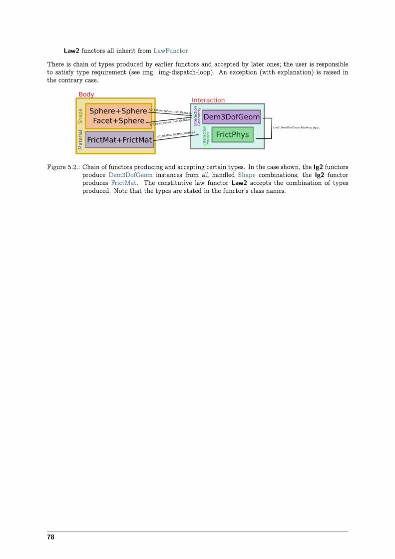
Law2 functors all inherit from LawFunctor.

There is chain of types produced by earlier functors and accepted by later ones; the user is responsibleto satisfy type requirement (see img. img-dispatch-loop). An exception (with explanation) is raised inthe contrary case.

Sphere+SphereFacet+Sphere Dem3DofGeom

FrictMat+FrictMatFrictPhys

Shape

Material

Ig2_Sphere_Sphere_Dem3DofGeom

Ig2_Facet_Sphere_

Dem3DofGeom

Ip2_FrictMat_FrictMa

t_FrictPhys

BodyInteraction

Interaction

Geometry

Interaction

Physics

Law2_Dem3DofGeom_FrictPhys_Basic

Figure 5.2.: Chain of functors producing and accepting certain types. In the case shown, the Ig2 functorsproduce Dem3DofGeom instances from all handled Shape combinations; the Ig2 functorproduces FrictMat. The constitutive law functor Law2 accepts the combination of typesproduced. Note that the types are stated in the functor’s class names.

78

6. User’s manual

6.1. Scene construction

6.1.1. Triangulated surfaces

Yade integrates with the the GNU Triangulated Surface library, exposed in python via th 3rd party gtsmodule. GTS provides variety of functions for surface manipuation (coarsening, tesselation, simlification,import), to be found in its documentation.

GTS surfaces are geometrical objects, which can be inserted into simulation as set of particles whoseBody.shape is of type Facet – single triangulation elements. pack.gtsSurface2Facets can be used to convertGTS surface triangulation into list of bodies ready to be inserted into simulation via O.bodies.append.

Facet particles are created by default as non-Body.dynamic (they have zero inertial mass). That meansthat they are fixed in space and will not move if subject to forces. You can however

• prescribe arbitrary movement to facets using a PartialEngine (such as TranslationEngine or Rota-tioNEngine);

• assign explicitly mass and inertia to that particle;

• make that particle part of a clump and assign mass and inertia of the clump itself (described below).

Note: Facets can only (currently) interact with spheres, not with other facets, even if they are dynamic.Collision of 2 facets will not create interaction, therefore no forces on facets.

6.1.1.1. Import

Yade currently offers 3 formats for importing triangulated surfaces from external files, in the ymportmodule:

ymport.gts text file in native GTS format.

ymport.stl STereoLitography format, in either text or binary form; exported from Blender, but frommany CAD systems as well.

ymport.gmsh. text file in native format for GMSH, popular open-source meshing program.

If you need to manipulate surfaces before creating list of facets, you can study the py/ymport.py filewhere the import functions are defined. They are rather simple in most cases.

6.1.1.2. Parametric construction

The gts module provides convenient way of creating surface by vertices, edges and triangles.

Frequently, though, the surface can be conveniently described as surface between polylines in space. Forinstance, cylinder is surface between two polygons (closed polylines). The pack.sweptPolylines2gtsSurfaceoffers the functionality of connecting several polylines with triangulation.

79

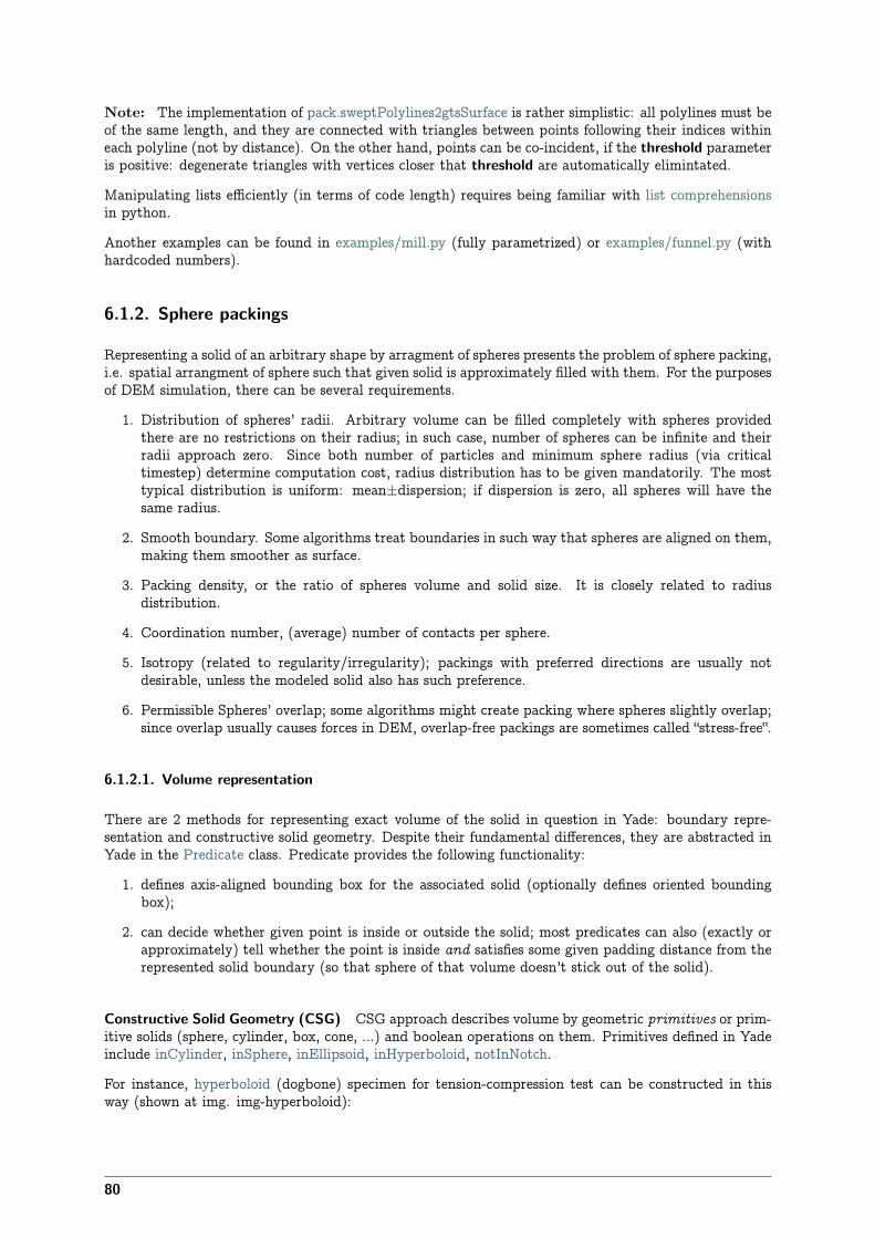
Note: The implementation of pack.sweptPolylines2gtsSurface is rather simplistic: all polylines must beof the same length, and they are connected with triangles between points following their indices withineach polyline (not by distance). On the other hand, points can be co-incident, if the threshold parameteris positive: degenerate triangles with vertices closer that threshold are automatically elimintated.

Manipulating lists efficiently (in terms of code length) requires being familiar with list comprehensionsin python.

Another examples can be found in examples/mill.py (fully parametrized) or examples/funnel.py (withhardcoded numbers).

6.1.2. Sphere packings

Representing a solid of an arbitrary shape by arragment of spheres presents the problem of sphere packing,i.e. spatial arrangment of sphere such that given solid is approximately filled with them. For the purposesof DEM simulation, there can be several requirements.

1. Distribution of spheres’ radii. Arbitrary volume can be filled completely with spheres providedthere are no restrictions on their radius; in such case, number of spheres can be infinite and theirradii approach zero. Since both number of particles and minimum sphere radius (via criticaltimestep) determine computation cost, radius distribution has to be given mandatorily. The mosttypical distribution is uniform: mean±dispersion; if dispersion is zero, all spheres will have thesame radius.

2. Smooth boundary. Some algorithms treat boundaries in such way that spheres are aligned on them,making them smoother as surface.

3. Packing density, or the ratio of spheres volume and solid size. It is closely related to radiusdistribution.

4. Coordination number, (average) number of contacts per sphere.

5. Isotropy (related to regularity/irregularity); packings with preferred directions are usually notdesirable, unless the modeled solid also has such preference.

6. Permissible Spheres’ overlap; some algorithms might create packing where spheres slightly overlap;since overlap usually causes forces in DEM, overlap-free packings are sometimes called “stress-free‟.

6.1.2.1. Volume representation

There are 2 methods for representing exact volume of the solid in question in Yade: boundary repre-sentation and constructive solid geometry. Despite their fundamental differences, they are abstracted inYade in the Predicate class. Predicate provides the following functionality:

1. defines axis-aligned bounding box for the associated solid (optionally defines oriented boundingbox);

2. can decide whether given point is inside or outside the solid; most predicates can also (exactly orapproximately) tell whether the point is inside and satisfies some given padding distance from therepresented solid boundary (so that sphere of that volume doesn’t stick out of the solid).

Constructive Solid Geometry (CSG) CSG approach describes volume by geometric primitives or prim-itive solids (sphere, cylinder, box, cone, …) and boolean operations on them. Primitives defined in Yadeinclude inCylinder, inSphere, inEllipsoid, inHyperboloid, notInNotch.

For instance, hyperboloid (dogbone) specimen for tension-compression test can be constructed in thisway (shown at img. img-hyperboloid):

80

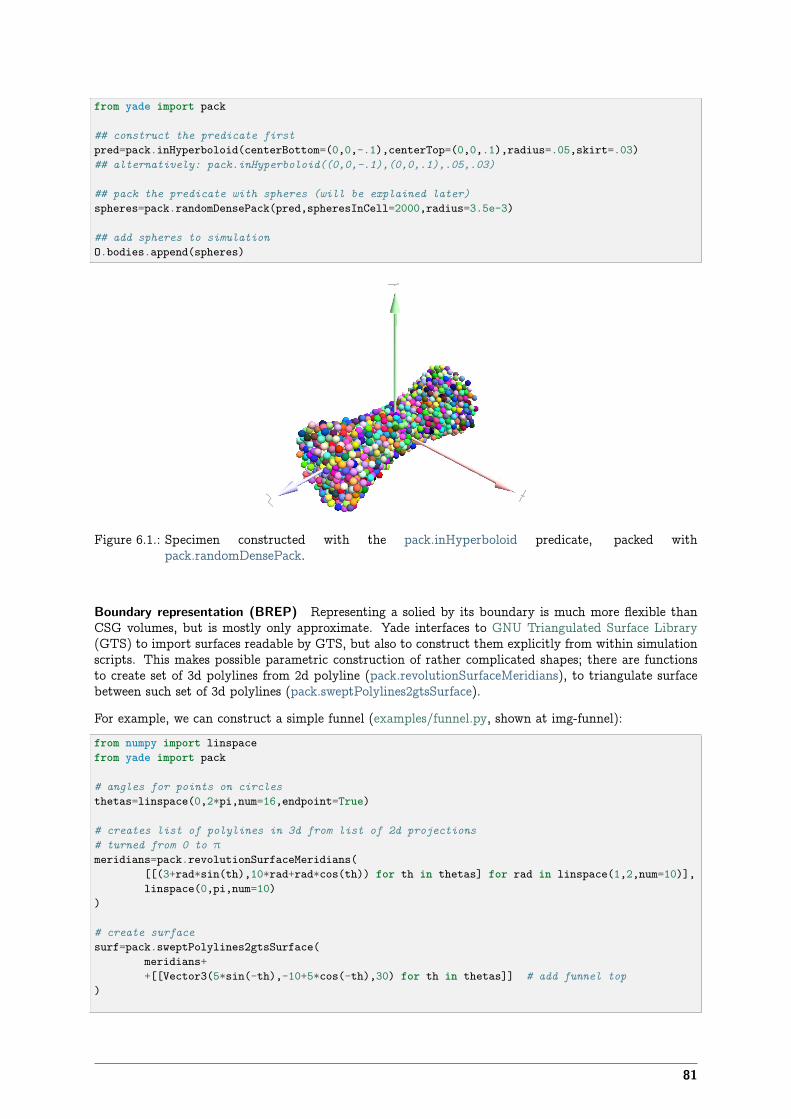
from yade import pack

## construct the predicate firstpred=pack.inHyperboloid(centerBottom=(0,0,-.1),centerTop=(0,0,.1),radius=.05,skirt=.03)## alternatively: pack.inHyperboloid((0,0,-.1),(0,0,.1),.05,.03)

## pack the predicate with spheres (will be explained later)spheres=pack.randomDensePack(pred,spheresInCell=2000,radius=3.5e-3)

## add spheres to simulationO.bodies.append(spheres)

Figure 6.1.: Specimen constructed with the pack.inHyperboloid predicate, packed withpack.randomDensePack.

Boundary representation (BREP) Representing a solied by its boundary is much more flexible thanCSG volumes, but is mostly only approximate. Yade interfaces to GNU Triangulated Surface Library(GTS) to import surfaces readable by GTS, but also to construct them explicitly from within simulationscripts. This makes possible parametric construction of rather complicated shapes; there are functionsto create set of 3d polylines from 2d polyline (pack.revolutionSurfaceMeridians), to triangulate surfacebetween such set of 3d polylines (pack.sweptPolylines2gtsSurface).

For example, we can construct a simple funnel (examples/funnel.py, shown at img-funnel):from numpy import linspacefrom yade import pack

# angles for points on circlesthetas=linspace(0,2*pi,num=16,endpoint=True)

# creates list of polylines in 3d from list of 2d projections# turned from 0 to π

meridians=pack.revolutionSurfaceMeridians([[(3+rad*sin(th),10*rad+rad*cos(th)) for th in thetas] for rad in linspace(1,2,num=10)],linspace(0,pi,num=10)

)

# create surfacesurf=pack.sweptPolylines2gtsSurface(

meridians++[[Vector3(5*sin(-th),-10+5*cos(-th),30) for th in thetas]] # add funnel top

)

81

# add to simulationO.bodies.append(pack.gtsSurface2Facets(surf))

Figure 6.2.: Triangulated funnel, constructed with the examples/funnel.py script.

GTS surface objects can be used for 2 things:

1. pack.gtsSurface2Facets function can create the triangulated surface (from Facet particles) in thesimulation itself, as shown in the funnel example. (Triangulated surface can also be importeddirectly from a STL file using ymport.stl.)

2. pack.inGtsSurface predicate can be created, using the surface as boundary representation of theenclosed volume.

The scripts/test/gts-horse.py (img. img-horse) shows both possibilities; first, a GTS surface is imported:import gtssurf=gts.read(open('horse.coarse.gts'))

That surface object is used as predicate for packing:

pred=pack.inGtsSurface(surf)O.bodies.append(pack.regularHexa(pred,radius=radius,gap=radius/4.))

and then, after being translated, as base for triangulated surface in the simulation itself:

surf.translate(0,0,-(aabb[1][2]-aabb[0][2]))O.bodies.append(pack.gtsSurface2Facets(surf,wire=True))

Boolean operations on predicates Boolean operations on pair of predicates (noted A and B) are defined:

• intersection A & B (conjunction): point must be in both predicates involved.

• union A | B (disjunction): point must be in both predicates involved.

• difference A - B (conjunction with second predicate negated): the point must be in the firstpredicate and not in the second one.

• symmetric difference A ^ B (exclusive disjunction): point must be in exactly one of the twopredicates.

Composed predicates also properly define their bounding box. For example, we can take box and removecylinder from inside, using the A - B operation (img. img-predicate-difference):

82

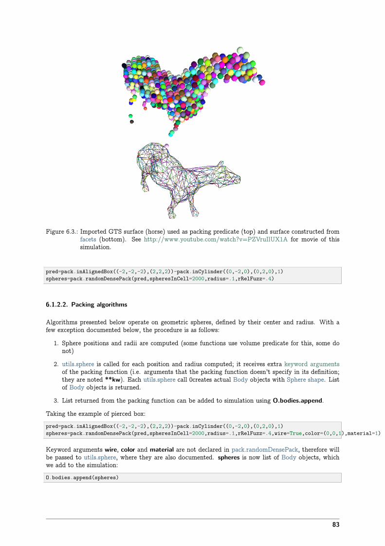
Figure 6.3.: Imported GTS surface (horse) used as packing predicate (top) and surface constructed fromfacets (bottom). See http://www.youtube.com/watch?v=PZVruIlUX1A for movie of thissimulation.

pred=pack.inAlignedBox((-2,-2,-2),(2,2,2))-pack.inCylinder((0,-2,0),(0,2,0),1)spheres=pack.randomDensePack(pred,spheresInCell=2000,radius=.1,rRelFuzz=.4)

6.1.2.2. Packing algorithms

Algorithms presented below operate on geometric spheres, defined by their center and radius. With afew exception documented below, the procedure is as follows:

1. Sphere positions and radii are computed (some functions use volume predicate for this, some donot)

2. utils.sphere is called for each position and radius computed; it receives extra keyword argumentsof the packing function (i.e. arguments that the packing function doesn’t specify in its definition;they are noted **kw). Each utils.sphere call 0creates actual Body objects with Sphere shape. Listof Body objects is returned.

3. List returned from the packing function can be added to simulation using O.bodies.append.

Taking the example of pierced box:

pred=pack.inAlignedBox((-2,-2,-2),(2,2,2))-pack.inCylinder((0,-2,0),(0,2,0),1)spheres=pack.randomDensePack(pred,spheresInCell=2000,radius=.1,rRelFuzz=.4,wire=True,color=(0,0,1),material=1)

Keyword arguments wire, color and material are not declared in pack.randomDensePack, therefore willbe passed to utils.sphere, where they are also documented. spheres is now list of Body objects, whichwe add to the simulation:

O.bodies.append(spheres)

83

Figure 6.4.: Box with cylinder removed from inside, using difference of these two predicates.

Packing algorithms described below produce dense packings. If one needs loose packing, pack.SpherePackclass provides functions for generating loose packing, via its pack.SpherePack.makeCloud method. It isused internally for generating initial configuration in dynamic algorithms. For instance:from yade import packsp=pack.SpherePack()sp.makeCloud(minCorner=(0,0,0),maxCorner=(3,3,3),rMean=.2,rRelFuzz=.5)

will fill given box with spheres, until no more spheres can be placed. The object can be used to addspheres to simulation:

for c,r in sp: O.bodies.append(utils.sphere(c,r))

or, in a more pythonic way, with one single O.bodies.append call:

O.bodies.append([utils.sphere(c,r) for c,r in sp])

Geometric Geometric algorithms compute packing without performing dynamic simulation; amoghtheir advantages are

• speed;

• spheres touch exactly, there are no overlaps (what some people call “stress-free” packing);

their chief disadvantage is that radius distribution cannot be prescribed exactly, save in specific cases(regular packings); sphere radii are given by the algorithm, which already makes the system determined.If exact radius distribuition is important for your problem, consider dynamic algorithms instead.

Regular Yade defines packing generators for spheres with constant radii, which can be used with volumepredicates as described above. They are dense orthogonal packing (pack.regularOrtho) and dense hexag-onal packing (pack.regularHexa). The latter creates so-called “hexagonal close packing”, which achievesmaximum density (http://en.wikipedia.org/wiki/Close-packing_of_spheres).

Clear disadvantage of regular packings is that they have very strong directional preferences, which mightnot be an issue in some cases.

84

Irregular Random geometric algorithms do not integrate at all with volume predicates described above;rather, they take their own boundary/volume definition, which is used during sphere positioning. Onthe other hand, this makes it possible for them to respect boundary in the sense of making spheres touchit at appropriate places, rather than leaving empty space in-between.

SpherePadder constructs dense sphere packing based on pre-computed tetrahedron mesh; it is doc-umented in SpherePadder documentation; sample script is in scripts/test/SpherePadder.py.SpherePadder does not return Body list as other algorithms, but a pack.SpherePack object; itcan be iterated over, adding spheres to the simulation, as shown in its documentation.

GenGeo is library (python module) for packing generation developed with ESyS-Particle. It createspacking by random insertion of spheres with given radius range. Inserted spheres touch each otherexactly and, more importantly, they also touch the boundary, if in its neighbourhood. Boundaryis represented as special object of the GenGeo library (Sphere, cylinder, box, convex polyhedron,…). Therefore, GenGeo cannot be used with volume represented by yade predicates as explainedabove.

Packings generated by this module can be imported directly via ymport.gengeo, or from saved filevia ymport.gengeoFile. There is an example script scripts/test/genCylLSM.py. Full documentationfor GenGeo can be found at ESyS documentation website.

To our knowledge, the GenGeo library is not currently packaged. It can be downloaded from currentsubversion repository

svn checkout https://svn.esscc.uq.edu.au/svn/esys3/lsm/contrib/LSMGenGeo

then following instruction in the INSTALL file.

Dynamic The most versatile algorithm for random dense packing is provided bypack.randomDensePack. Initial loose packing of non-overlapping spheres is generated by randomlyplacing placing them in cuboid volume, with radii given by requested (currently only uniform) radiusdistribution. When no more spheres can be inserted, the packing is compressed, then uncompressed (seepy/pack.py for exact values of these “stresses”), byt running a DEM simulation; Omega.switchWorld isused to not affect existing simulation). Finally, resulting packing is clipped using provided predicate, asexplained above.

By its nature, this method might take relatively long; and there are 2 provisions to make the computationtime shorter:

• If number of spheres using the spheresInCell parameter is specified, only smaller specimen withperiodic boundary is created and then repeated as to fill the predicate. This can provide high-quality packing with low regularity, depending on the spheresInCell parameter (value of severalthousands is recommended).

• Providing memoizeDb parameter will make pack.randomDensePack first look into provided file(SQLite database) for packings with similar parameters. On success, the packing is simply readfrom database and returned. If there is no similar pre-existent packing, normal procedure is run,and the result is saved in the database before being returned, so that subsequent calls with sameparameters will return quickly.

If you need to obtain full periodic packing (rather than packing clipped by predicate), you can usepack.randomPeriPack.

In case of specific needs, you can create packing yourself, “by hand”. For instance, packing boundary canbe constructed from facets, letting randomly positioned spheres in space fall down under gravity.

6.1.3. Adding particles

The BodyContainer holds Body objects in the simulation; it is accessible as O.bodies.

85

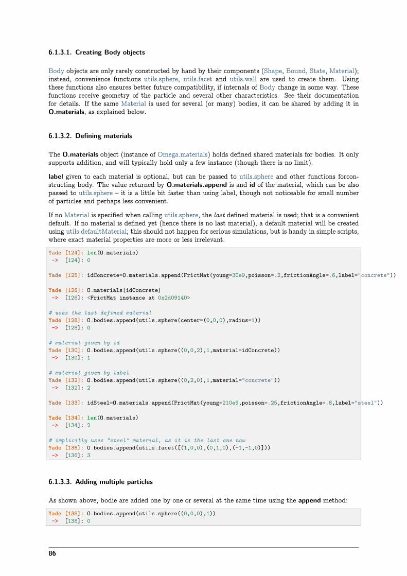
6.1.3.1. Creating Body objects

Body objects are only rarely constructed by hand by their components (Shape, Bound, State, Material);instead, convenience functions utils.sphere, utils.facet and utils.wall are used to create them. Usingthese functions also ensures better future compatibility, if internals of Body change in some way. Thesefunctions receive geometry of the particle and several other characteristics. See their documentationfor details. If the same Material is used for several (or many) bodies, it can be shared by adding it inO.materials, as explained below.

6.1.3.2. Defining materials

The O.materials object (instance of Omega.materials) holds defined shared materials for bodies. It onlysupports addition, and will typically hold only a few instance (though there is no limit).

label given to each material is optional, but can be passed to utils.sphere and other functions forcon-structing body. The value returned by O.materials.append is and id of the material, which can be alsopassed to utils.sphere – it is a little bit faster than using label, though not noticeable for small numberof particles and perhaps less convenient.

If no Material is specified when calling utils.sphere, the last defined material is used; that is a convenientdefault. If no material is defined yet (hence there is no last material), a default material will be createdusing utils.defaultMaterial; this should not happen for serious simulations, but is handy in simple scripts,where exact material properties are more or less irrelevant.

Yade [124]: len(O.materials)-> [124]: 0

Yade [125]: idConcrete=O.materials.append(FrictMat(young=30e9,poisson=.2,frictionAngle=.6,label="concrete"))

Yade [126]: O.materials[idConcrete]-> [126]: <FrictMat instance at 0x2d09140>

# uses the last defined materialYade [128]: O.bodies.append(utils.sphere(center=(0,0,0),radius=1))-> [128]: 0

# material given by idYade [130]: O.bodies.append(utils.sphere((0,0,2),1,material=idConcrete))-> [130]: 1

# material given by labelYade [132]: O.bodies.append(utils.sphere((0,2,0),1,material="concrete"))-> [132]: 2

Yade [133]: idSteel=O.materials.append(FrictMat(young=210e9,poisson=.25,frictionAngle=.8,label="steel"))

Yade [134]: len(O.materials)-> [134]: 2

# implicitly uses "steel" material, as it is the last one nowYade [136]: O.bodies.append(utils.facet([(1,0,0),(0,1,0),(-1,-1,0)]))-> [136]: 3

6.1.3.3. Adding multiple particles

As shown above, bodie are added one by one or several at the same time using the append method:

Yade [138]: O.bodies.append(utils.sphere((0,0,0),1))-> [138]: 0

86

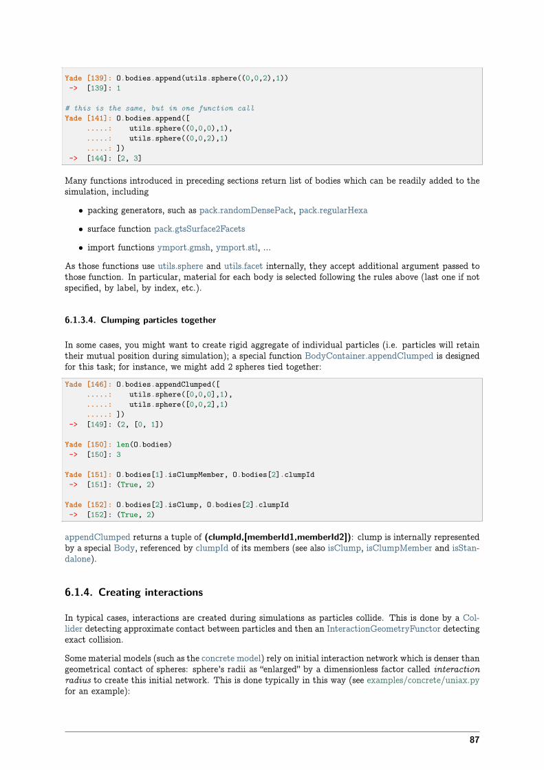
Yade [139]: O.bodies.append(utils.sphere((0,0,2),1))-> [139]: 1

# this is the same, but in one function callYade [141]: O.bodies.append([

.....: utils.sphere((0,0,0),1),

.....: utils.sphere((0,0,2),1)

.....: ])-> [144]: [2, 3]

Many functions introduced in preceding sections return list of bodies which can be readily added to thesimulation, including

• packing generators, such as pack.randomDensePack, pack.regularHexa

• surface function pack.gtsSurface2Facets

• import functions ymport.gmsh, ymport.stl, …

As those functions use utils.sphere and utils.facet internally, they accept additional argument passed tothose function. In particular, material for each body is selected following the rules above (last one if notspecified, by label, by index, etc.).

6.1.3.4. Clumping particles together

In some cases, you might want to create rigid aggregate of individual particles (i.e. particles will retaintheir mutual position during simulation); a special function BodyContainer.appendClumped is designedfor this task; for instance, we might add 2 spheres tied together:

Yade [146]: O.bodies.appendClumped([.....: utils.sphere([0,0,0],1),.....: utils.sphere([0,0,2],1).....: ])

-> [149]: (2, [0, 1])

Yade [150]: len(O.bodies)-> [150]: 3

Yade [151]: O.bodies[1].isClumpMember, O.bodies[2].clumpId-> [151]: (True, 2)

Yade [152]: O.bodies[2].isClump, O.bodies[2].clumpId-> [152]: (True, 2)

appendClumped returns a tuple of (clumpId,[memberId1,memberId2]): clump is internally representedby a special Body, referenced by clumpId of its members (see also isClump, isClumpMember and isStan-dalone).

6.1.4. Creating interactions

In typical cases, interactions are created during simulations as particles collide. This is done by a Col-lider detecting approximate contact between particles and then an InteractionGeometryFunctor detectingexact collision.

Some material models (such as the concrete model) rely on initial interaction network which is denser thangeometrical contact of spheres: sphere’s radii as “enlarged” by a dimensionless factor called interactionradius to create this initial network. This is done typically in this way (see examples/concrete/uniax.pyfor an example):

87

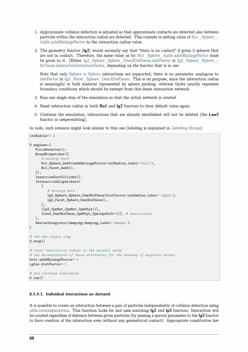
1. Approximate collision detection is adjusted so that approximate contacts are detected also betweenparticles within the interaction radius are detected. This consists in setting value of Bo1_Sphere_-Aabb.aabbEnlargeFactor to the interaction radius value.

2. The geometry functor (Ig2) would normally say that “there is no contact” if given 2 spheres thatare not in contact. Therefore, the same value as for Bo1_Sphere_Aabb.aabbEnlargeFactor mustbe given to it. (Either Ig2_Sphere_Sphere_Dem3DofGeom.distFactor or Ig2_Sphere_Sphere_-ScGeom.interactionDetectionFactor, depending on the functor that is in use.

Note that only Sphere + Sphere interactions are supported; there is no parameter analogous todistFactor in Ig2_Facet_Sphere_Dem3DofGeom. This is on purpose, since the interaction radiusis meaningful in bulk material represented by sphere packing, whereas facets usually representboundary conditions which should be exempt from this dense interaction network.

3. Run one single step of the simulation so that the initial network is created.

4. Reset interaction radius in both Bo1 and Ig2 functors to their default value again.

5. Continue the simulation; interactions that are already established will not be deleted (the Law2functor in usepermitting).

In code, such scenario might look similar to this one (labeling is explained in Labeling things):intRadius=1.5

O.engines=[ForceResetter(),BoundDispatcher([

# enlarge hereBo1_Sphere_Aabb(aabbEnlargeFactor=intRadius,label='bo1s'),Bo1_Facet_Aabb(),

]),InsertionSortCollider(),InteractionDispatchers(

[# enlarge hereIg2_Sphere_Sphere_Dem3DofGeom(distFactor=intRadius,label='ig2ss'),Ig2_Facet_Sphere_Dem3DofGeom(),

],[Ip2_CpmMat_CpmMat_CpmPhys()],[Law2_Dem3DofGeom_CpmPhys_Cpm(epsSoft=0)], # deactivated

),NewtonIntegrator(damping=damping,label='damper'),

]

# run one single stepO.step()

# reset interaction radius to the default value# see documentation of those attributes for the meaning of negative valuesbo1s.aabbEnlargeFactor=-1ig2ss.distFactor=-1

# now continue simulationO.run()

6.1.4.1. Individual interactions on demand

It is possible to create an interaction between a pair of particles independently of collision detection usingutils.createInteraction. This function looks for and uses matching Ig2 and Ip2 functors. Interaction willbe created regardless of distance between given particles (by passing a special parameter to the Ig2 functorto force creation of the interaction even without any geometrical contact). Appropriate constitutive law

88

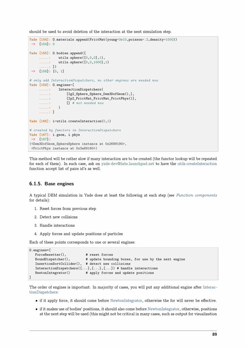
should be used to avoid deletion of the interaction at the next simulation step.

Yade [154]: O.materials.append(FrictMat(young=3e10,poisson=.2,density=1000))-> [154]: 0

Yade [155]: O.bodies.append([.....: utils.sphere([0,0,0],1),.....: utils.sphere([0,0,1000],1).....: ])

-> [158]: [0, 1]

# only add InteractionDispatchers, no other engines are needed nowYade [159]: O.engines=[

.....: InteractionDispatchers(

.....: [Ig2_Sphere_Sphere_Dem3DofGeom(),],

.....: [Ip2_FrictMat_FrictMat_FrictPhys()],

.....: [] # not needed now

.....: )

.....: ]

Yade [166]: i=utils.createInteraction(0,1)

# created by functors in InteractionDispatchersYade [167]: i.geom, i.phys-> [167]:(<Dem3DofGeom_SphereSphere instance at 0x2699190>,<FrictPhys instance at 0x3a69160>)

This method will be rather slow if many interaction are to be created (the functor lookup will be repeatedfor each of them). In such case, ask on yade-dev@lists.launchpad.net to have the utils.createInteractionfunction accept list of pairs id’s as well.

6.1.5. Base engines

A typical DEM simulation in Yade does at least the following at each step (see Function componentsfor details):

1. Reset forces from previous step

2. Detect new collisions

3. Handle interactions

4. Apply forces and update positions of particles

Each of these points corresponds to one or several engines:

O.engines=[ForceResetter(), # reset forcesBoundDispatcher(), # update bounding boxes, for use by the next engineInsertionSortCollider(), # detect new collisionsInteractionDispatchers([...],[...],[...]) # handle interactionsNewtonIntegrator() # apply forces and update positions

]

The order of engines is important. In majority of cases, you will put any additional engine after Interac-tionDispatchers:

• if it apply force, it should come before NewtonIntegrator, otherwise the for will never be effective.

• if it makes use of bodies’ positions, it should also come before NewtonIntegrator, otherwise, positionsat the next step will be used (this might not be critical in many cases, such as output for visualization

89

with VTKRecorder).

The O.engines sequence must be always assigned at once (the reason is in the fact that although enginesthemselves are passed by reference, the sequence is copied from c++ to Python or from Python to c++).This includes modifying an existing O.engines; therefore

O.engines.append(SomeEngine()) # wrong

will not work;

O.engines=O.engines+[SomeEngine()] # ok

must be used instead. For inserting an engine after position #2 (for example), use python slice notation:

O.engines=O.engines[:2]+[SomeEngine()]+O.engines[2:]

6.1.5.1. Functors choice

In the above example, we omited functors, only writing ellipses ... instead. As explained in Dispatchersand functors, there are 4 kinds of functors and associated dispatchers. User can choose which ones touse, though the choice must be consistent.

Bo1 functors Bo1 functors must be chosen depending on the collider in use.

At this moment (May 2010), the most common choice is InsertionSortCollider, which uses Aabb; functorscreating Aabb must be used in that case. Depending on particle shapes in your simulation, chooseappropriate functors:

O.engines=[...,BoundDispatcher([Bo1_Sphere_Aabb(),Bo1_Facet_Aabb()]),InsertionSortCollider(),...

]

Using more functors than necessary (such as Bo1_Facet_Aabb if there are no facets in the simulation)has no performance penalty. On the other hand, missing functors for existing shapes will cause thosebodies to not collider with other bodies (they will freely interpenetrate).

There are other colliders as well, though their usage is only experimental:

• SpatialQuickSortCollider is correctness-reference collider operating on Aabb; it is significantlyslower than InsertionSortCollider.

• PersistentTriangulationCollider only works on spheres; it does not use a BoundDispatcher, as itoperates on spheres directly.

• FlatGridCollider is proof-of-concept grid-based collider, which computes grid positions internally(no BoundDispatcher either)

Ig2 functors Ig2 functor choice (all of the derive from InteractionGeometryFunctor) depends on

1. shape combinations that should collide; for instance:

InteractionDispatchers([Ig2_Sphere_Sphere_Dem3DofGeom()],[],[])

will handle collisions for Sphere + Sphere, but not for Facet + Sphere – if that is desired, anadditional functor must be used:

90

InteractionDispatchers([Ig2_Sphere_Sphere_Dem3DofGeom(),Ig2_Facet_Sphere_Dem3DofGeom()

],[],[])

Again, missing combination will cause given shape combinations to freely interpenetrate one an-other.

2. InteractionGeometry type accepted by the Law2 functor (below); it is the first part of functor’sname after Law2 (for instance, Law2_Dem3DofGeom_CpmPhys_Cpm accepts Dem3DofGeom).This is (for most cases) either Dem3DofGeom (total shear formulation) or ScGeom (incrementalshear formulation). For ScGeom, the above example would simply change to:

InteractionDispatchers([Ig2_Sphere_Sphere_ScGeom(),Ig2_Facet_Sphere_ScGeom()

],[],[])

Ip2 functors Ip2 functors (deriving from InteractionPhysicsFunctor) must be chosen depending on

1. Material combinations within the simulation. In most cases, Ip2 functors handle 2 instances of thesame Material class (such as Ip2_FrictMat_FrictMat_FrictPhys for 2 bodies with FrictMat)

2. InteractionPhysics accepted by the constitutive law (Law2 functor), which is the second part of theLaw2 functor’s name (e.g. Law2_ScGeom_FrictPhys_Basic accepts FrictPhys)

Note: Unlike with Bo1 and Ig2 functors, unhandled combination of Materials is an error conditionsignaled by an exception.

Law2 functor(s) Law2 functor was the ultimate criterion for the choice of Ig2 and Ig2 functors; thereare no restrictions on its choice in itself, as it only applies forces without creating new objects.

In most simulations, only one Law2 functor will be in use; it is possible, though, to have several of them,dispatched based on combination of InteractionGeometry and InteractionPhysics produced previously byIg2 and Ip2 functors respectively (in turn based on combination of Shapes and Materials).

Note: As in the case of Ip2 functors, receiving a combination of InteractionGeometry and Interaction-Physics which is not handled by any Law2 functor is an error.

Examples Let us give several example of the chain of created and accepted types.

Basic DEM model Suppose we want to use the Law2_ScGeom_FrictPhys_Basic constitutive law. Wesee that

1. the Ig2 functors most create ScGeom. Since we have spheres and walls in the simulation, wewill need functors accepting Sphere + Sphere and Wall + Sphere combinations. We don’t wantinteractions between walls themselves (as a matter of fact, there is no such functor anyway). Thatgives us Ig2_Sphere_Sphere_ScGeom and Ig2_Wall_Sphere_ScGeom (as a matter of facet, thereis no such functor now, although it is planned)

2. the Ip2 functors should create FrictPhys. Looking at InteractionPhysicsFunctors, there is onlyIp2_FrictMat_FrictMat_FrictPhys. That obliges us to use FrictMat for particles.

The result will be therefore:

InteractionDispatchers([Ig2_Sphere_Sphere_ScGeom(),Ig2_Wall_Sphere_ScGeom()],[Ip2_FrictMat_FrictMat_FrictPhys()],

91

[Law2_ScGeom_FrictPhys_Basic()])

Concrete model In this case, our goal is to use the Law2_Dem3DofGeom_CpmPhys_Cpm constitutivelaw.

• We use spheres and facets in the simulation, which selects Ig2 functors accepting those typesand producing Dem3DofGeom: Ig2_Sphere_Sphere_Dem3DofGeom and Ig2_Facet_Sphere_-Dem3DofGeom.

• We have to use Material which can be used for creating CpmPhys. We find that CpmPhys is onlycreated by Ip2_CpmMat_CpmMat_CpmPhys, which determines the choice of CpmMat for allparticles.

Therefore, we will use:

InteractionDispatchers([Ig2_Sphere_Sphere_Dem3DofGeom(),Ig2_Facet_Sphere_Dem3DofGeom()],[Ip2_CpmMat_CpmMat_CpmPhys()],[Law2_Dem3DofGeom_CpmPhys_Cpm()]

)

6.1.6. Imposing conditions

In most simulations, it is not desired that all particles float freely in space. There are several ways ofimposing boundary conditions that block movement of all or some particles with regard to global space.

6.1.6.1. Motion constraints

• Body.dynamic determines whether a body will be moved by NewtonIntegrator; it is mandatory forbodies with zero mass, where applying non-zero force would result in infinite displacement.

Facets are case in the point: utils.facet makes them non-dynamic by default, as they have zerovolume and zero mass (this can be changed, by passing dynamic-True to utils.facet or settingBody.dynamic; setting State.mass to a non-zero value must be done as well). The same is true forutils.wall.

Making sphere non-dynamic is achieved simply by:

utils.sphere([x,y,z],radius,dynamic=False)

Note: There is an open bug #398089 to define exactly what the dynamic flag does. Please readit before writing a new engine relying on this flag.

• State.blockedDOFs permits selective blocking of any of 6 degrees of freedom in global space. Forinstance, a sphere can be made to move only in the xy plane by saying:

Yade [169]: O.bodies.append(utils.sphere((0,0,0),1))-> [169]: 0

Yade [170]: O.bodies[0].state.blockedDOFs=['z','rx','ry']

In contrast to Body.dynamic, blockedDOFs will only block forces (and acceleration) in that direc-tion being effective; if you prescribed linear or angular velocity, they will be applied regardless ofblockedDOFs. (This is also related to bug #398089 mentioned above)

It might be desirable to constrain motion of some particles constructed from a generated sphere packing,following some condition, such as being at the bottom of a specimen; this can be done by looping over

92

all bodies with a conditional:for b in O.bodies:

# block all particles with z coord below .5:if b.state.pos[2]<.5: b.dynamic=False

Arbitrary spatial predicates introduced above can be expoited here as well:from yade import packpred=pack.inAlignedBox(lowerCorner,upperCorner)for b in O.bodies:

if b.shape.name!=Sphere: continue # skip non-spheres# ask the predicate if we are insideif pred(b.state.pos,b.shape.radius): b.dynamic=False

6.1.6.2. Boundary controllers

Engines deriving from BoundaryController impose boundary conditions during simulation, either directly,or by influencing several bodies. You are referred to their individual documentation for details, thoughyou might find interesting in particular

• UniaxialStrainer for applying strain along one axis at constant rate; useful for plotting strain-stressdiagrams for uniaxial loading case. See examples/concrete/uniax.py for an example.

• TriaxialStressController which applies prescribed stress/strain along 3 perpendicular axes oncuboid-shaped packing using 6 walls (Box objects) (ThreeDTriaxialEngine is generalized such thatit allows independent value of stress along each axis)

• PeriTriaxController for applying stress/strain along 3 axes independently, for simulations usingperiodic boundary conditions (Cell)

6.1.6.3. Field appliers

Engines deriving from FieldApplier acting on all particles. The one most used is GravityEngine applyinguniform acceleration field.

6.1.6.4. Partial engines

Engines deriving from PartialEngine define the subscribedBodies attribute determining bodies which willbe affected. Several of them warrant explicit mention here:

• TranslationEngine and RotationEngine for applying constant speed linear and rotational motionon subscribers.

• ForceEngine and TorqueEngine applying given values of force/torque on subscribed bodies at everystep.

• StepDisplacer for applying generalized displacement delta at every timestep; designed for precisecontrol of motion when testing constitutive laws on 2 particles.

If you need an engine applying non-constant value instead, there are several interpolating engines (Inter-polatingDirectedForceEngine for applying force with varying magnitude, InterpolatingSpiralEngine forapplying spiral displacement with varying angular velocity and possibly others); writing a new interpo-lating engine is rather simple using examples of those that already exist.

6.1.7. Convenience features

93

6.1.7.1. Labeling things

Engines and functors can define that label attribute. Whenever the O.engines sequence is modified,python variables of those names are created/update; since it happens in the __builtins__ namespaces,these names are immediately accessible from anywhere. This was used in Creating interactions to changeinteraction radius in multiple functors at once.

Warning: Make sure you do not use label that will overwrite (or shadow) an object that you alreadyuse under that variable name. Take care not to use syntactically wrong names, such as “er*452” or“my engine”; only variable names permissible in Python can be used.

6.1.7.2. Simulation tags

Omega.tags is a dictionary (it behaves like a dictionary, although the implementation in c++ is different)mapping keys to labels. Contrary to regular python dictionaries that you could create,

• O.tags is saved and loaded with simulation;

• O.tags has some values pre-initialized.

After Yade startup, O.tags contains the following:

Yade [172]: dict(O.tags) # convert to real dictionary-> [172]:{'author': 'V??clav~??milauer~(vaclav@flux)','description': '','id': '20100531T100723p5665','isoTime': '20100531T100723'}

author Real name, username and machine as obtained from your system at simulation creation

id Unique identifier of this Yade instance (or of the instance which created a loded simulation). It iscomposed of date, time and process number. Useful if you run simulations in parallel and want toavoid overwriting each other’s outputs; embed O.tags[’id’] in output filenames (either as directoryname, or as part of the file’s name itself) to avoid it. This is explained in batch-output-separatein detail.

isoTime Time when simulation was created (with second resolution).

You can add your own tags by simply assigning value, with the restriction that the left-handside objectmust be a string:

Yade [173]: O.tags['anythingThat I lik3']='whatever'

Yade [174]: O.tags['anythingThat I lik3']-> [174]: 'whatever'

6.1.7.3. Saving python variables

Python variable lifetime is limited; in particular, if you save simulation, variables will be lost afterreloading. Yade provides limited support for data persistence for this reason (internally, it uses specialvalues of O.tags). The functions in question are utils.saveVars and utils.loadVars.

utils.saveVars takes dictionary (variable names and their values) and a mark (identification string forthe variable set); it saves the dictionary inside the simulation. These variables can be re-created (afterthe simulation was loaded from a XML file, for instance) in the __builtin__ namespace by callingutils.loadVars with the same identification mark:

94

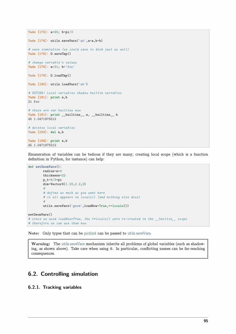
Yade [175]: a=45; b=pi/3

Yade [176]: utils.saveVars('ab',a=a,b=b)

# save simulation (we could save to disk just as well)Yade [176]: O.saveTmp()

# change variable's valuesYade [176]: a=21; b='foo'

Yade [179]: O.loadTmp()

Yade [180]: utils.loadVars('ab')

# GOTCHA! Local variables shadow builtin variablesYade [181]: print a,b21 foo

# these are our builtins nowYade [181]: print __builtins__.a, __builtins__.b45 1.0471975512

# deletes local variablesYade [183]: del a,b

Yade [184]: print a,b45 1.0471975512

Enumeration of variables can be tedious if they are many; creating local scope (which is a functiondefinition in Python, for instance) can help:

def setGeomVars():radius=a*4thickness=22p_t=4/3*pidim=Vector3(1.23,2.2,3)## define as much as you want here# it all appears in locals() (and nothing else does)#utils.saveVars('geom',loadNow=True,**locals())

setGeomVars()# since we used loadNow=True, the **locals() were re-created in the __builtin__ scope# therefore we can use them now

Note: Only types that can be pickled can be passed to utils.saveVars.

Warning: The utils.saveVars mechanism inherits all problems of global variables (such as shadow-ing, as shown above). Take care when using it. In particular, conflicting names can he far-reachingconsequences.

6.2. Controlling simulation

6.2.1. Tracking variables

95

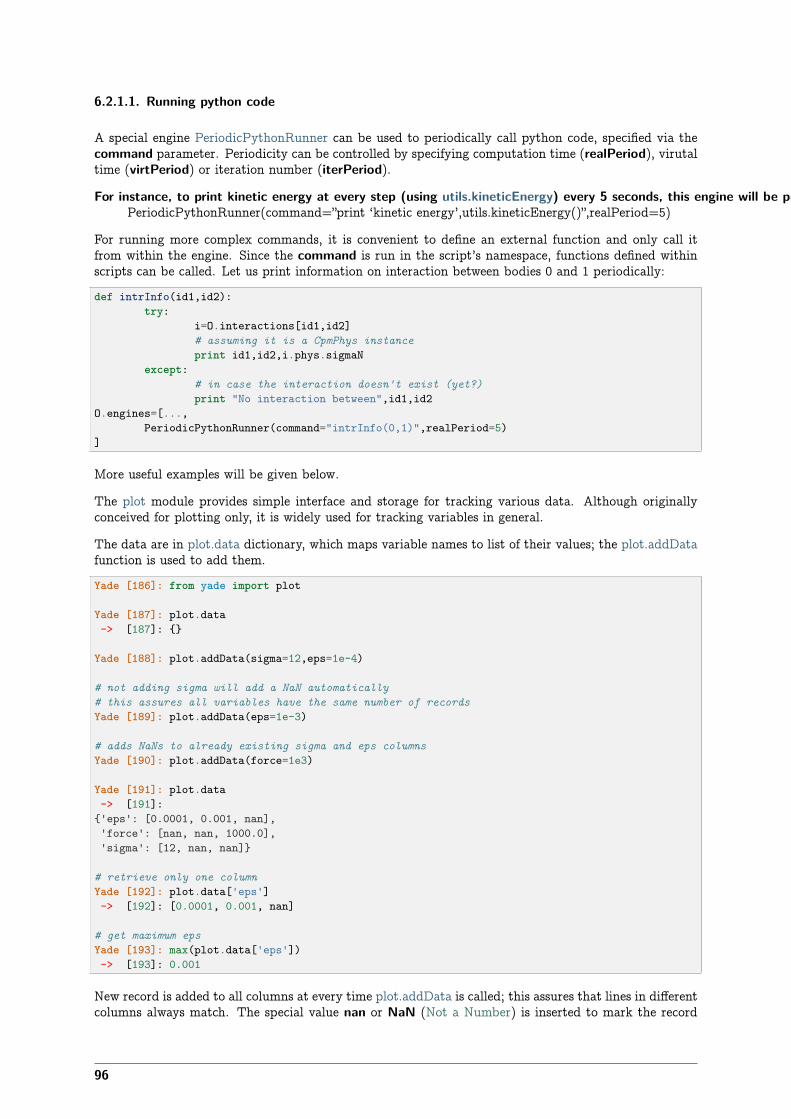
6.2.1.1. Running python code

A special engine PeriodicPythonRunner can be used to periodically call python code, specified via thecommand parameter. Periodicity can be controlled by specifying computation time (realPeriod), virutaltime (virtPeriod) or iteration number (iterPeriod).

For instance, to print kinetic energy at every step (using utils.kineticEnergy) every 5 seconds, this engine will be put to O.engines::PeriodicPythonRunner(command=”print ‘kinetic energy’,utils.kineticEnergy()”,realPeriod=5)

For running more complex commands, it is convenient to define an external function and only call itfrom within the engine. Since the command is run in the script’s namespace, functions defined withinscripts can be called. Let us print information on interaction between bodies 0 and 1 periodically:

def intrInfo(id1,id2):try:

i=O.interactions[id1,id2]# assuming it is a CpmPhys instanceprint id1,id2,i.phys.sigmaN

except:# in case the interaction doesn't exist (yet?)print "No interaction between",id1,id2

O.engines=[...,PeriodicPythonRunner(command="intrInfo(0,1)",realPeriod=5)

]

More useful examples will be given below.

The plot module provides simple interface and storage for tracking various data. Although originallyconceived for plotting only, it is widely used for tracking variables in general.

The data are in plot.data dictionary, which maps variable names to list of their values; the plot.addDatafunction is used to add them.

Yade [186]: from yade import plot

Yade [187]: plot.data-> [187]: {}

Yade [188]: plot.addData(sigma=12,eps=1e-4)

# not adding sigma will add a NaN automatically# this assures all variables have the same number of recordsYade [189]: plot.addData(eps=1e-3)

# adds NaNs to already existing sigma and eps columnsYade [190]: plot.addData(force=1e3)

Yade [191]: plot.data-> [191]:{'eps': [0.0001, 0.001, nan],'force': [nan, nan, 1000.0],'sigma': [12, nan, nan]}

# retrieve only one columnYade [192]: plot.data['eps']-> [192]: [0.0001, 0.001, nan]

# get maximum epsYade [193]: max(plot.data['eps'])-> [193]: 0.001

New record is added to all columns at every time plot.addData is called; this assures that lines in differentcolumns always match. The special value nan or NaN (Not a Number) is inserted to mark the record

96

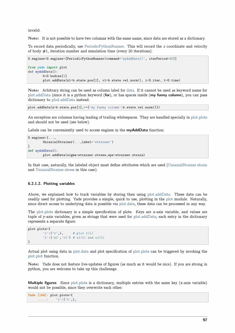
invalid.

Note: It is not possible to have two columns with the same name, since data are stored as a dictionary.

To record data periodically, use PeriodicPythonRunner. This will record the z coordinate and velocityof body #1, iteration number and simulation time (every 20 iterations):

O.engines=O.engines+[PeriodicPythonRunner(command='myAddData()', iterPeriod=20)]

from yade import plotdef myAddData():

b=O.bodies[1]plot.addData(z1=b.state.pos[2], v1=b.state.vel.norm(), i=O.iter, t=O.time)

Note: Arbitrary string can be used as column label for data. If it cannot be used as keyword name forplot.addData (since it is a python keyword (for), or has spaces inside (my funny column), you can passdictionary to plod.addData instead:

plot.addData(z=b.state.pos[2],**{'my funny column':b.state.vel.norm()})

An exception are columns having leading of trailing whitespaces. They are handled specially in plot.plotsand should not be used (see below).

Labels can be conveniently used to access engines in the myAddData function:

O.engines=[...,UniaxialStrainer(...,label='strainer')

]def myAddData():

plot.addData(sigma=strainer.stress,eps=strainer.strain)

In that case, naturally, the labeled object must define attributes which are used (UniaxialStrainer.strainand UniaxialStrainer.stress in this case).

6.2.1.2. Plotting variables

Above, we explained how to track variables by storing then using plot.addData. These data can bereadily used for plotting. Yade provides a simple, quick to use, plotting in the plot module. Naturally,since direct access to underlying data is possible via plot.data, these data can be processed in any way.

The plot.plots dictionary is a simple specification of plots. Keys are x-axis variable, and values aretuple of y-axis variables, given as strings that were used for plot.addData; each entry in the dictionaryrepresents a separate figure:

plot.plots={'i':('t',), # plot t(i)'t':('z1','v1') # z1(t) and v1(t)

}

Actual plot using data in plot.data and plot specification of plot.plots can be triggered by invoking theplot.plot function.

Note: Yade does not feature live-updates of figures (as much as it would be nice). If you are strong inpython, you are welcome to take up this challenege.

Multiple figures Since plot.plots is a dictionary, multiple entries with the same key (x-axis variable)would not be possible, since they overwrite each other:

Yade [194]: plot.plots={.....: 'i':('t',),

97

.....: 'i':('z1','v1')

.....: }

Yade [198]: plot.plots-> [198]: {'i': ('z1', 'v1')}

You can, however, distinguish them by prepending/appending space to the x-axis variable, which will beremoved automatically when looking for the variable in plot.data – both x-axes will use the i column:

Yade [199]: plot.plots={.....: 'i':('t',),.....: 'i ':('z1','v1') # note the space in 'i '.....: }

Yade [203]: plot.plots-> [203]: {'i': ('t',), 'i ': ('z1', 'v1')}

Split y1 y2 axes To avoid big range differences on the y axis, it is possible to have left and right y axesseparate (like axes x1y2 in gnuplot). This is achieved by inserting None to the plot specifier; variablescoming before will be plot normally (on the left y-axis), while those after will appear on the right:

plot.plots={'i':('z1',None,'v1')}

Exporting Plots can be exported to external files for later post-processing via that plot.saveGnuplotfunction.

• Data file is saved (compressed using bzip2) separately from the gnuplot file, so any other programscan be used to process them. In particular, the numpy.genfromtxt (documented here) can be usefulto import those data back to python; the decompression happens automatically.

• The gnuplot file can be run through gnuplot to produce the figure; see plot.saveGnuplot documen-tation for details.

6.2.2. Stop conditions

For simulations with pre-determined number of steps, number of steps can be prescribed:

# absolute iteration number O.stopAtIter=35466 O.run() O.wait()

or# number of iterations to run from nowO.run(35466,True) # wait=True

causes the simulation to run 35466 iterations, then stopping.

Frequently, decisions have to be made based on evolution of the simulation itself, which is not yet known.In such case, a function checking some specific condition is called periodically; if the condition is satisfied,O.pause or other functions can be called to stop the stimulation. See documentation for Omega.run,Omega.pause, Omega.step, Omega.stopAtIter for details.

For simulations that seek static equilibrium, the _utils.unbalancedForce can provide a useful metrics (seeits documentation for details); for a desired value of 1e-2 or less, for instance, we can use:

def checkUnbalanced():if utils.unbalancedForce<1e-2: O.pause()

O.engines=O.engines+[PeriodicPythonRunner(command="checkUnbalanced",iterPeriod=100)]

98

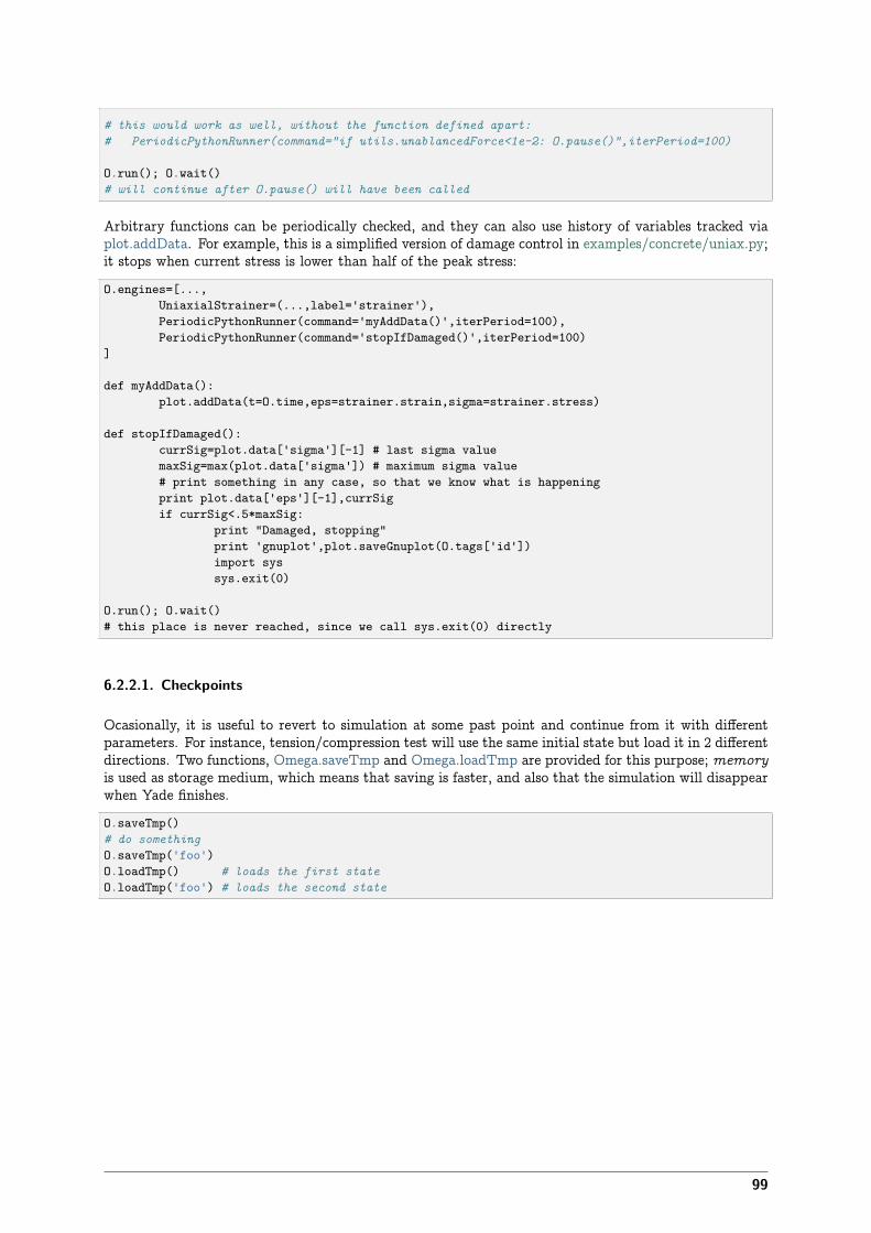
# this would work as well, without the function defined apart:# PeriodicPythonRunner(command="if utils.unablancedForce<1e-2: O.pause()",iterPeriod=100)

O.run(); O.wait()# will continue after O.pause() will have been called

Arbitrary functions can be periodically checked, and they can also use history of variables tracked viaplot.addData. For example, this is a simplified version of damage control in examples/concrete/uniax.py;it stops when current stress is lower than half of the peak stress:

O.engines=[...,UniaxialStrainer=(...,label='strainer'),PeriodicPythonRunner(command='myAddData()',iterPeriod=100),PeriodicPythonRunner(command='stopIfDamaged()',iterPeriod=100)

]

def myAddData():plot.addData(t=O.time,eps=strainer.strain,sigma=strainer.stress)

def stopIfDamaged():currSig=plot.data['sigma'][-1] # last sigma valuemaxSig=max(plot.data['sigma']) # maximum sigma value# print something in any case, so that we know what is happeningprint plot.data['eps'][-1],currSigif currSig<.5*maxSig:

print "Damaged, stopping"print 'gnuplot',plot.saveGnuplot(O.tags['id'])import syssys.exit(0)

O.run(); O.wait()# this place is never reached, since we call sys.exit(0) directly

6.2.2.1. Checkpoints

Ocasionally, it is useful to revert to simulation at some past point and continue from it with differentparameters. For instance, tension/compression test will use the same initial state but load it in 2 differentdirections. Two functions, Omega.saveTmp and Omega.loadTmp are provided for this purpose; memoryis used as storage medium, which means that saving is faster, and also that the simulation will disappearwhen Yade finishes.

O.saveTmp()# do somethingO.saveTmp('foo')O.loadTmp() # loads the first stateO.loadTmp('foo') # loads the second state

99

Warning: O.loadTmp cannot be called from inside an engine, since before loading a simulation,the old one must finish the current iteration; it would lead to deadlock, since O.loadTmp would waitfor the current iteration to finish, while the current iteration would be blocked on O.loadTmp.A special trick must be used: a separate function to be run after the current iteration is defined andis invoked from an independent thread launched only for that purpose:

O.engines=[...,PeriodicPythonRunner('myFunc()',iterPeriod=345)]

def myFunc():if someCondition:

import thread# the () are arguments passed to the functionthread.start_new_thread(afterIterFunc,())

def afterIterFunc():O.pause(); O.wait() # wait till the iteration really finishesO.loadTmp()

O.saveTmp()O.run()

6.2.3. Remote control

Yade can be controlled remotely over network. At yade startup, the following lines appear, among othermessages:TCP python prompt on localhost:9000, auth cookie `dcekyu'TCP info provider on localhost:21000

They inform about 2 ports on which connection of 2 different kind is accepted.

6.2.3.1. Python prompt

TCP python prompt is telnet server with authenticated connection, providing full python command-line.It listens on port 9000, or higher if already occupied (by another yade instance, for example).

Using the authentication cookie, connection can be made:

$ telnet localhost 9000Trying 127.0.0.1...Connected to localhost.Escape character is '^]'.Enter auth cookie: dcekyu__ __ ____ __ _____ ____ ____\ \ / /_ _| _ \ ___ ___ / / |_ _/ ___| _ \\ V / _` | | | |/ _ \ / _ \ / / | || | | |_) || | (_| | |_| | __/ | (_) / / | || |___| __/|_|\__,_|____/ \___| \___/_/ |_| \____|_|

(connected from 127.0.0.1:40372)>>>

The python pseudo-prompt >>> lets you write commands to manipulate simulation in variety of waysas usual. Two things to notice:

1. The new python interpreter (>>>) lives in a namespace separate from Yade [1]: command-line.For your convenience, from yade import * is run in the new python instance first, but local andglobal variables are not accessible (only builtins are).

100

2. The (fake) >>> interpreter does not have rich interactive feature of IPython, which handles theusual command-line Yade [1]:; therefore, you will have no command history, ? help and so on.

Note: By giving access to python interpreter, full control of the system (including reading user’s files) ispossible. For this reason, connection are only allowed from localhost, not over network remotely.

Warning: Authetication cookie is trivial to crack via bruteforce attack. Although the listenerstalls for 5 seconds after every failed login attempt (and disconnects), the cookie could be guessed bytrial-and-error during very long simulations on a shared computer.

6.2.3.2. Info provider

TCP Info provider listens at port 21000 (or higher) and returns some basic information about currentsimulation upon connection; the connection terminates immediately afterwards. The information ispython dictionary represented as string (serialized) using standard pickle module.

This functionality is used by the batch system (described below) to be informed about individual sim-ulation progress and estimated times. If you want to access this information yourself, you can studycore/main/yade-multi.in for details.

6.2.4. Batch queuing and execution (yade-multi)

Yade features light-weight system for running one simulation with different parameters; it handles as-signment of parameter values to python variables in simulation script, scheduling jobs based on numberof available and required cores and more. The whole batch consists of 2 files:

simulation script regular Yade script, which calls utils.readParamsFromTable to obtain parameters fromparameter table. In order to make the script runnable outside the batch, readParamsFromTabletakes default values of parameters, which might be overridden from the parameter table.

utils.readParamsFromTable knows which parameter file and which line to read by inspecting thePARAM_TABLE environment variable, set by the batch system.

parameter table simple text file, each line representing one parameter set. This file is read byutils.readParamsFromTable (using utils.TableParamReader class), called from simulation script,as explained above.

The batch can be run asyade-multi parameters.table simulation.py

and it will intelligently run one simulation for each parameter table line.

6.2.4.1. Example

This example is found in scripts/multi.table and scripts/multi.py.

Suppsoe we want to study influence of parameters density and initialVelocity on position of a spherefalling on fixed box. We create parameter table like this:description density initialVelocity # first non-empty line are column headingsreference 2400 10hi_v = 20 # = to use value from previous linelo_v = 5# comments are allowedhi_rho 5000 10# blank lines as well:

101

hi_rho_v = 20hi_rh0_lo_v = 5

Each line give one combination of these 2 parameters and assigns (which is optional) a description ofthis simulation.

In the simulation file, we read parameters from table, at the beginning of the script; each parameter hasdefault value, which is used if not specified in the parameters file:from yade import utilsutils.readParamsFromTable(

gravity=-9.81,density=2400,initialVelocity=20,noTableOk=True # use default values if not run in batch

)print gravity, density, initialVelocity

after the call to utils.readParamsFromTable, corresponding python variables are created and can bereadily used in the script, e.g.

GravityEngine(gravity=(0,0,gravity))

Warning: New variables are created in the builtin namespace, in order to be visible from every-where. Avoid name clash with existing variables, such as Vector3 or time, your script might berendered unfunctional.

Let us see what happens when running the batch:

$ yade-multi multi.table multi.pyWill run `/usr/local/bin/yade-trunk' on `multi.py' with nice value 10, output redirected to `multi.@.log', 4 jobs at a time.Will use table `multi.table', with available lines 2, 3, 4, 5, 6, 7.Will use lines 2 (reference), 3 (hi_v), 4 (lo_v), 5 (hi_rho), 6 (hi_rho_v), 7 (hi_rh0_lo_v).Master process pid 7030

These lines inform us about general batch information: nice level, log file names, how many cores will beused (4); table name, and line numbers that contain parameters; finally, which lines will be used; masterPID is useful for killing (stopping) the whole batch with the kill command.Job summary:

#0 (reference/4): PARAM_TABLE=multi.table:2 DISPLAY= /usr/local/bin/yade-trunk --threads=4 --nice=10 -x multi.py > multi.reference.log 2>&1#1 (hi_v/4): PARAM_TABLE=multi.table:3 DISPLAY= /usr/local/bin/yade-trunk --threads=4 --nice=10 -x multi.py > multi.hi_v.log 2>&1#2 (lo_v/4): PARAM_TABLE=multi.table:4 DISPLAY= /usr/local/bin/yade-trunk --threads=4 --nice=10 -x multi.py > multi.lo_v.log 2>&1#3 (hi_rho/4): PARAM_TABLE=multi.table:5 DISPLAY= /usr/local/bin/yade-trunk --threads=4 --nice=10 -x multi.py > multi.hi_rho.log 2>&1#4 (hi_rho_v/4): PARAM_TABLE=multi.table:6 DISPLAY= /usr/local/bin/yade-trunk --threads=4 --nice=10 -x multi.py > multi.hi_rho_v.log 2>&1#5 (hi_rh0_lo_v/4): PARAM_TABLE=multi.table:7 DISPLAY= /usr/local/bin/yade-trunk --threads=4 --nice=10 -x multi.py > multi.hi_rh0_lo_v.log 2>&1

displays all jobs with command-lines that will be run for each of them. At this moment, the batch startsto be run.

#0 (reference/4) started on Tue Apr 13 13:59:32 2010#0 (reference/4) done (exit status 0), duration 00:00:01, log multi.reference.log#1 (hi_v/4) started on Tue Apr 13 13:59:34 2010#1 (hi_v/4) done (exit status 0), duration 00:00:01, log multi.hi_v.log#2 (lo_v/4) started on Tue Apr 13 13:59:35 2010#2 (lo_v/4) done (exit status 0), duration 00:00:01, log multi.lo_v.log#3 (hi_rho/4) started on Tue Apr 13 13:59:37 2010#3 (hi_rho/4) done (exit status 0), duration 00:00:01, log multi.hi_rho.log#4 (hi_rho_v/4) started on Tue Apr 13 13:59:38 2010#4 (hi_rho_v/4) done (exit status 0), duration 00:00:01, log multi.hi_rho_v.log#5 (hi_rh0_lo_v/4) started on Tue Apr 13 13:59:40 2010

102

#5 (hi_rh0_lo_v/4) done (exit status 0), duration 00:00:01, log multi.hi_rh0_lo_v.log

information about job status changes is being printed, until:All jobs finished, total time 00:00:08Log files:multi.reference.log multi.hi_v.log multi.lo_v.log multi.hi_rho.log multi.hi_rho_v.log multi.hi_rh0_lo_v.logBye.

6.2.4.2. Separating output files from jobs

As one might output data to external files during simulation (using classes such as VTKRecorder, it isimportant to name files in such way that they are not overwritten by next (or concurrent) job in the samebatch. A special tag O.tags[’id’] is provided for such purposes: it is comprised of date, time and PID,which makes it always unique (e.g. 20100413T144723p7625); additional advantage is that alphabeticalorder of the id tag is also chronological.

For smaller simulations, prepending all output file names with O.tags[’id’] can be sufficient:

utils.saveGnuplot(O.tags['id'])

For larger simulations, it is advisable to create separate directory of that name first, putting all filesinside afterwards:

os.mkdir(O.tags['id'])O.engines=[

# …VTKRecorder(fileName=O.tags['id']+'/'+'vtk'),# …

]# …O.saveGnuplot(O.tags['id']+'/'+'graph1')

6.2.4.3. Controlling parallel compuation

Default total number of available cores is determined from /proc/cpuinfo (provided by Linux kernel); inaddition, if OMP_NUM_THREADS environment variable is set, minimum of these two is taken. The-j/--jobs option can be used to override this number.

By default, each job uses all available cores for itself, which causes jobs to be effectively run in parallel.Number of cores per job can be globally changed via the --job-threads option.

Table column named !OMP_NUM_THREADS (! prepended to column generally means to assignenvironment variable, rather than python variable) controls number of threads for each job separately,if it exists.

If number of cores for a job exceeds total number of cores, warning is issued and only the total numberof cores is used instead.

6.2.4.4. Merging gnuplot from individual jobs

Frequently, it is desirable to obtain single figure for all jobs in the batch, for comparison purposes.Somewhat heiristic way for this functionality is provided by the batch system. yade-multi must be runwith the --gnuplot option, specifying some file name that will be used for the merged figure:yade-trunk --gnuplot merged.gnuplot multi.table multi.py

103

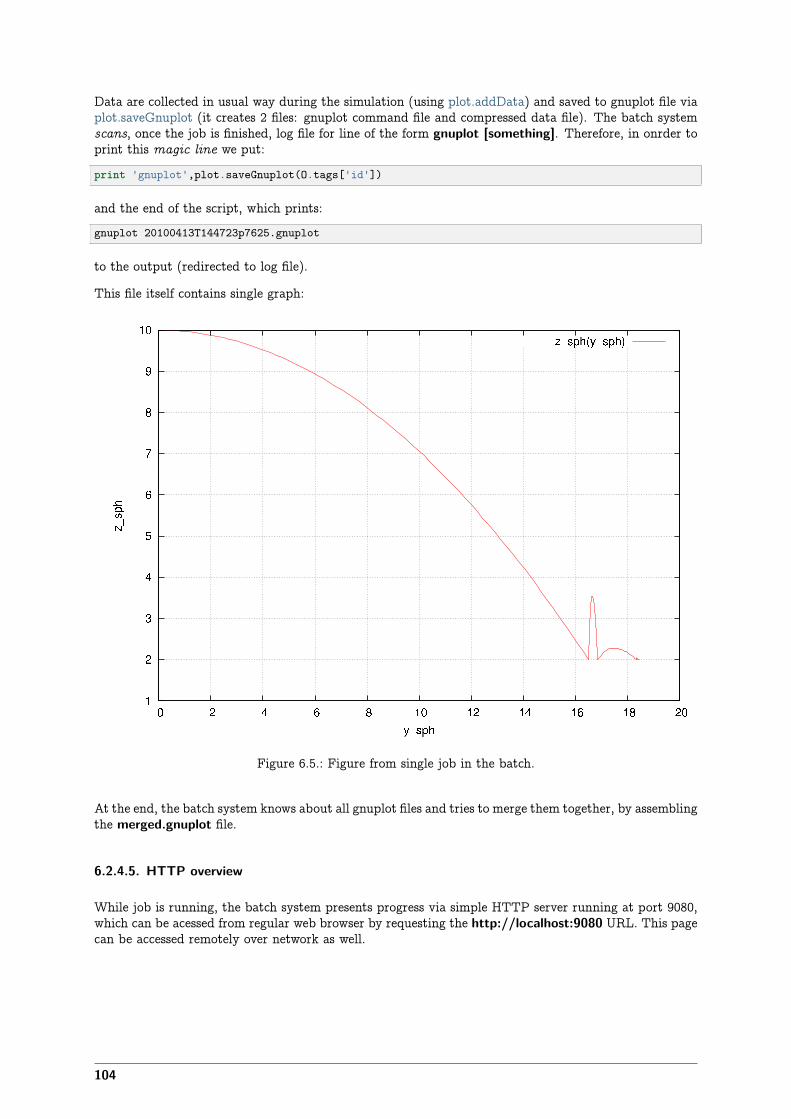
Data are collected in usual way during the simulation (using plot.addData) and saved to gnuplot file viaplot.saveGnuplot (it creates 2 files: gnuplot command file and compressed data file). The batch systemscans, once the job is finished, log file for line of the form gnuplot [something]. Therefore, in onrder toprint this magic line we put:

print 'gnuplot',plot.saveGnuplot(O.tags['id'])

and the end of the script, which prints:gnuplot 20100413T144723p7625.gnuplot

to the output (redirected to log file).

This file itself contains single graph:

Figure 6.5.: Figure from single job in the batch.

At the end, the batch system knows about all gnuplot files and tries to merge them together, by assemblingthe merged.gnuplot file.

6.2.4.5. HTTP overview

While job is running, the batch system presents progress via simple HTTP server running at port 9080,which can be acessed from regular web browser by requesting the http://localhost:9080 URL. This pagecan be accessed remotely over network as well.

104

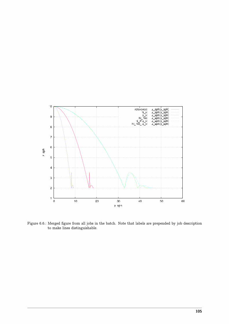
Figure 6.6.: Merged figure from all jobs in the batch. Note that labels are prepended by job descriptionto make lines distinguishable.

105

Figure 6.7.: Summary page available at port 9080 as batch is processed (updates every 5 seconds auto-matically). Possible job statuses are pending, running, done, failed.

106

6.3. Postprocessing

Not yet written. Describe how to use plot, post2d and VTKRecorder with Paraview.

6.4. Extending Yade

How to write new constitutive law: not yet written, see https://yade-dem.org/wiki/ConstitutiveLawHowto.

6.5. Troubleshooting

6.5.1. Crashes

It is possible that you encounter crash of Yade, i.e. Yade terminates with error message such as

Segmentation fault (core dumped)

without further explanation. Frequent causes of such conditions are

• program error in Yade itself;

• fatal condition in you particular simulation (such as impossible dispatch);

• problem with graphics card driver.

Try to reproduce the error (run the same script) with debug-enabled version of Yade. Debugger willbe automatically launched at crash, showing backtrace of the code (in this case, we triggered crash byhand):

Yade [1]: import os,signalYade [2]: os.kill(os.getpid(),signal.SIGSEGV)SIGSEGV/SIGABRT handler called; gdb batch file is `/tmp/yade-YwtfRY/tmp-0'GNU gdb (GDB) 7.1-ubuntuCopyright (C) 2010 Free Software Foundation, Inc.License GPLv3+: GNU GPL version 3 or later <http://gnu.org/licenses/gpl.html>This is free software: you are free to change and redistribute it.There is NO WARRANTY, to the extent permitted by law. Type "show copying"and "show warranty" for details.This GDB was configured as "x86_64-linux-gnu".For bug reporting instructions, please see:<http://www.gnu.org/software/gdb/bugs/>.[Thread debugging using libthread_db enabled][New Thread 0x7f0fb1268710 (LWP 16471)][New Thread 0x7f0fb29f2710 (LWP 16470)][New Thread 0x7f0fb31f3710 (LWP 16469)]

…

What looks as cryptic message is valuable information for developers to locate source of the bug. Inparticular, there is (usually) line <signal handler called>; lines below it are source of the bug (at leastvery likely so):

Thread 1 (Thread 0x7f0fcee53700 (LWP 16465)):#0 0x00007f0fcd8f4f7d in __libc_waitpid (pid=16497, stat_loc=<value optimized out>, options=0) at ../sysdeps/unix/sysv/linux/waitpid.c:41#1 0x00007f0fcd88c7e9 in do_system (line=<value optimized out>) at ../sysdeps/posix/system.c:149#2 0x00007f0fcd88cb20 in __libc_system (line=<value optimized out>) at ../sysdeps/posix/system.c:190#3 0x00007f0fcd0b4b23 in crashHandler (sig=11) at core/main/pyboot.cpp:45

107

#4 <signal handler called>#5 0x00007f0fcd87ed57 in kill () at ../sysdeps/unix/syscall-template.S:82#6 0x000000000051336d in posix_kill (self=<value optimized out>, args=<value optimized out>) at ../Modules/posixmodule.c:4046#7 0x00000000004a7c5e in call_function (f=Frame 0x1c54620, for file <ipython console>, line 1, in <module> (), throwflag=<value optimized out>) at ../Python/ceval.c:3750#8 PyEval_EvalFrameEx (f=Frame 0x1c54620, for file <ipython console>, line 1, in <module> (), throwflag=<value optimized out>) at ../Python/ceval.c:2412

If you think this might be error in Yade, file a bug report as explained below. Do not forget to attach fullyade output from terminal, including startup messages and debugger output – select with right moustbutton, paste with middle button to the bugreport to to a file and attach it. Attach your simulationscript as well.

6.5.2. Reporting bugs

Bugs are general name for defects (functionality shortcomings, misdocumentation, crashes) or featurerequests. They are tracked at http://bugs.launchpad.net/yade.

When reporting a new bug, be as specific as possible; state version of yade you use, sustem version andso on, as explained in the above section on crashes.

6.5.3. Getting help

6.5.3.1. Mailing lists

Yade has two mailing-lists. Both are hosted at http://www.launchpad.net and before posting, you mustregister to Launchpad and subscribe to the list by adding yourself to “team” of the same name runningthe list.

yade-users@lists.launchpad.net is general help list for Yade users. Add yourself to yade-users team sothat you can post messages. List archive is available.

yade-dev@lists.launchpad.net is for discussions about Yade development; you must be member of yade-dev team to post. This list is archived as well.

Read How To Ask Questions The Smart Way before posting. Do not forget to state what version ofyade you use (shown when you start yade), what operating system (such as Ubuntu 10.04), and if youhave done any local modifications to source code.

6.5.3.2. Questions and answers

Launchpad provides interface for giving questions at https://answers.launchpad.net/yade/ which you canuse instead of mailing lists; at the moment, it functionally somewhat overlaps with yade-users, but hasthe advantage of tracking whether a particular question has already been answered.

6.5.3.3. Wiki

http://www.yade-dem.org/wiki/

6.5.3.4. Private and/or paid support

You might contact developers by their private mail (rather than by mailing list) if you do not want todisclose details on the mailing list. This is also a suitable method for proposing financial reward forimplementation of a substantial feature that is not yet in Yade – typically, though, we will request this

108

feature to be part of the public codebase once completed, so that the rest of the community can benefitfrom it as well.

109

7. Programmer’s manual

7.1. Build system

Yade uses [scons] build system for managing the build process. It takes care of configuration, compilationand installation. SCons is written in python and its build scripts are in python, too. SCons completedocumentation can be found in its manual page.

7.1.1. Pre-build configuration

We use $ to denote build variable in strings in this section; in SCons script, they can be used eitherby writing $variable in strings passed to SCons functions, or obtained as attribute of the Environmentinstance env, i.e. env[’variable’]; we use the formed in running text here.

In order to allow parallel installation of multiple yade versions, the installation location follows thepattern $PREFIX/lib/yade$SUFFIX for libraries and $PREFIX/bin/yade$SUFFIX for executables (inthe following, we will refer only to the first one). $SUFFIX takes the form -$version$variant, whichfurther allows multiple different builds of the same version (typically, optimized and debug builds). Forinstance, the default debug build of version 0.5 would be installed in /usr/local/lib/yade-0.5-dbg/, theexecutable being /usr/local/bin/yade-0.5-dbg.

The build process takes place outside the source tree, in directory reffered to as $buildDir within thosescripts. By default, this directory is ../build-$SUFFIX.

Each build depends on a number of configuration parameters, which are stored in mutually independentprofiles. They are selected according to the profile argument to scons (by default, the last profileused, stored in scons.current-profile). Each profile remembers its non-default variables in scons.profile-$profile.

There is a number of configuration parameters; you can list all of them by scons -h. The following tablesummarizes only a few that are the most used.

PREFIX [default: /usr/local] installation prefix (PREFIX preprocessor macro; yade.config.prefix inpython

version [bzr revision (e.g. bzr1899)] first part of suffix (SUFFIX preprocessor macro; yade.config.suffixin python)]

variant [(empty)] second part of suffix

buildPrefix [..] where to create build-$SUFFIX directory

debug [False (0)] add debugging symbols to output, enable stack traces on crash

optimize [True (1)] optimize binaries (#defines NDEBUG; assertions eliminated; YADE_CAST andYADE_PTR_CAST are static casts rather than dynamic; LOG_TRACE and LOG_DEBUG areeliminated)

CPPPATH [/usr/include/vtk-5.2:/usr/include/vtk-5.4] additional colon-separated paths for prepro-cessor (for atypical header locations). Required by some libraries, such as VTK (reflected bythe default)

111

LIBPATH [(empty)] additional colon-separated paths for linker

CXX [g++] compiler executable

CXXFLAGS [(empty)] additional compiler flags (may are added automatically)

jobs [4] number of concurrent compilations to run

brief [True (1)] only show brief notices about what is being done rather than full command-lines duringcompilation

linkStrategy [monolithic] whether to link all plugins in one shared library (monolithic) or in one fileper plugin (per-class); the first option is faster for overall builds, while the latter one makesrecompilation of only part of Yade faster; granularity of monolithic build can be changed with thechunkSize parameter, which determines how many files are compiled at once.

features [log4cxx,opengl,gts,openmp] optional comma-separated features to build with (details below;each defines macro YADE_$FEATURE; available as lowercased list yade.config.features at runtime

7.1.1.1. Library detection

When the scons command is run, it first checks for presence of all required libraries. Some of them areessential, other are optional and will be required only if features that need them are enabled.

Essentials

compiler Obviously c++ compiler is necessary. Yade relies on several extensions of g++ from the [gcc]suite and cannot (probably) be built with other compilers.

boost [boost] is a large collection of peer-reviewed c++ libraries. Yade currently uses thread, date_time,filesystem, iostreams, regex, serialization, program_options, foreach, python; typically the wholeboost bundle will be installed. If you need functionality from other modules, you can make presenceof that module mandatory. Only be careful about relying on very new features; due to range ofsystems yade is or might be used on, it is better to be moderately conservative (read: roughly 3years backwards compatibility).

python [python] is the scripting language used by yade. Besides [boost::python]_, yade further requires

• [ipython] (terminal interaction)

• [matplotlib] (plotting)

• [numpy] (matlab-like numerical functionality and accessing numpy arrays from c/c++ effi-ciently)

Optional libraries (features) The features parameter controls optional functionality. Each enabledfeature defines preprocessor macro YADE_FEATURE (name uppercased) to enable selective ex-clude/include of parts of code. In some cases, it would be meaningless to compile some file at all(e.g. VTKRecorder without the vtk feature). This can be controller using the YADE_REQUIRE_-FEATURE places in the respective implementation file (see the Linking section for more details).

log4cxx (YADE_LOG4CXX) Enable flexible logging system ([log4cxx]), which permits to assign log-ging levels on per-class basis; doesn’t change API, only redefines LOG_INFO and other macrosaccordingly; see log4cxx for details.

opengl (YADE_OPENGL) Enable 3d rendering as well as the Qt3-based graphical user interface (inaddition to python console).

vtk (YADE_VTK) Enable functionality using Visualization Toolkit ([vtk]; e.g. VTKRecorder exportingto files readable with ParaView).

112

openmp (YADE_OPENMP) Enable parallelization using OpenMP, non-intrusive shared-memory par-allelization framework; it is only supported for g++ > 4.0. Parallel computation leads to significantperformance increase and should be enabled unless you have a special reason for not doing so (e.g.single-core machine). See upyade-parallel for details.

gts (YADE_GTS) Enable functionality provided by GNU Triangulated Surface library ([gts]) and buildPyGTS, its python interface; used for surface import and construction.

cgal (YADE_CGAL) Enable functionality provided by Computation Geometry Algorithms Library([cgal]); triangulation code in MicroMacroAnalyser and PersistentTriagulationCollider ses its rou-tines.

other There might be more features added in the future. Always refer to scons -h output for possiblevalues.

Warning: Due to a long-standing bug in log4cxx, using log4cxx will make yade crash at every exit.We work-around this partially by disabling the crash handler for regular exits, but process exit statuswill still be non-zero. The batch system (yade-multi) detects successful runs by looking at magicline “Yade: normal exit.” in the process’ standard output.

Before compilation, SCons will check for presence of libraries required by their respective features 1.Failure will occur if a respective library isn’t found. To find out what went wrong, you can inspect../build-$SUFFIX/config.log file; it contains exact commands and their output for all performed checks.

Note: Features are not auto-detected on purpose; otherwise problem with library detection might buildYade without expected features, causing specifically problems for automatized builds.

7.1.2. Building

Yade source tree has the following structure (omiting debian, doc, examples and scripts which don’tparticipate in the build process); we shall call each top-level component module:

attic/ ## code that is not currently functional and might be removed unless resurrectedlattice/ ## lattice and lattice-like modelssnow/ ## snow model (is really a DEM)

core/ ## core simulation building blocksextra/ ## miscillaneagui/ ## user interfaces

qt3/ ## graphical user interface based on qt3 and OpenGLpy/ ## python console interface (phased out)

lib/ ## support libraries, not specific to simulationspkg/ ## simulation-specific files

common/ ## generally useful classesdem/ ## classes for Discrete Element Method

py/ ## python modules

Each directory on the top of this hierarchy (except pkg, which is treated specially – see below) containsfile SConscript, determining what files to compile, how to link them together and where should they beinstalled. Within these script, a scons variable env (build Environment) contains all the configurationparameters, which are used to influence the build process; they can be either obtained with the [] operator,but scons also replaces $var strings automatically in arguments to its functions:

if 'opengl' in env['features']:env.Install('$PREFIX/lib/yade$SUFFIX/',[

# ...])

1 Library checks are defined inside the SConstruct file and you can add your own, should you need it.

113

7.1.2.1. Header installation

To allow flexibility in source layout, SCons will copy (symlink) all headers into flattened structure withinthe build directory. First 2 components of the original directory are joind by dash, deeper levels arediscarded (in case of core and extra, only 1 level is used). The following table makes gives a fewexamples:

Original header location Included ascore/Scene.hpp <yade/core/Scene.hpp>lib/base/Logging.hpp <yade/lib-base/Logging.hpp>lib/serialization/Serializable.hpp <yade/lib-serialization/Serializable.hpp>pkg/dem/DataClass/SpherePack.hpp <yade/pkg-dem/SpherePack.hpp>gui/qt3/QtGUI.hpp <yade/gui-qt3/QtGUI.hpp>

It is advised to use #include<yade/module/Class.hpp> style of inclusion rather than #in-clude”Class.hpp even if you are in the same directory.

7.1.2.2. What files to compile

SConscript files in lib, core, gui, py and extra explicitly determine what files will be built.

Automatic compilation In the pkg/ directory, situation is different. In order to maximally ease additionof modules to yade, all *.cpp files are automatically scanned by SCons and considered for compilation.Each file may contain multiple lines that declare features that are necessary for this file to be compiled:

YADE_REQUIRE_FEATURE(vtk);YADE_REQUIRE_FEATURE(gts);

This file will be compiled only if both vtk and gts features are enabled. Depending on current featureset, only selection of plugins will be compiled.

It is possible to disable compilation of a file by requiring any non-existent feature, such as:

YADE_REQUIRE_FEATURE(temporarily disabled 345uiysdijkn);

The YADE_REQUIRE_FEATURE macro expands to nothing during actual compilation.

Note: The source scanner was written by hand and is not official part of SCons. It is fairly primitive andin particular, it doesn’t interpret c preprocessor macros, except for a simple non-nested feature-checkslike #ifdef YADE_*/#ifndef YADE_* #endif.

7.1.2.3. Linking

The order in which modules might depend on each other is given as follows:

mod-ule

resulting shared library dependencies

lib libyade-support.so can depend on external libraries, may not depend on anyother part of Yade.

core libcore.so yade-support; may depend on external libraries.pkg libplugins.so for monolithic

builds, libClass.so for per-class(per-plugin) builds.

core, yade-support; may not depend on external librariesexplcitly (only implicitly, by adding the library to globallinker flags in SConstruct)

ex-tra

(undefined) (arbitrary)

gui libQtGUI.so, libPythonUI.so lib, core, pkgpy (many files) lib, core, pkg, external

114

Because pkg plugins might be linked differently depending on the linkStrategy option, SConscript filesthat need to explicitly declare the dependency should use provided linkPlugins function which returnslibraries in which given plugins will be defined:

env.SharedLibrary('_packSpheres',['_packSpheres.cpp'],SHLIBPREFIX='',LIBS=env['LIBS']+[linkPlugins(['Shop','SpherePack']),]

),

Note: env[’LIBS’] are libraries that all files are linked to and they should always be part of the LIBSparameter.

Since plugins in pkg are not declared in any SConscript file, other plugins they dependon are again found automatically by scannig their #include directives for the pattern #in-clude<yade/module/Plugin.hpp>. Again, this works well in normal circumastances, but is not neces-sarily robust.

See scons manpage for meaning of parameters passed to build functions, such as SHLIBPREFIX.

7.2. Conventions

The following rules that should be respected; documentation is treated separately.

• general

– C++ source files have .hpp and .cpp extensions (for headers and implementation, respectively).

– All header files should have the #pragma once multiple-inclusion guard.

– Try to avoid using namespace … in header files.

– Use tabs for indentation. While this is merely visual in c++, it has semantic meaning inpython; inadverently mixing tabs and spaces can result in syntax errors.

• capitalization style

– Types should be always capitalized. Use CamelCase for composed names (GlobalEngine).Underscores should be used only in special cases, such as functor names.

– Class data members and methods must not be capitalized, composed names should use uselowercased camelCase (glutSlices). The same applies for functions in python modules.

– Preprocessor macros are uppercase, separated by underscores; those that are used outside thecore take (with exceptions) the form YADE_*, such as YADE_CLASS_BASE_DOC_*macro family.

• programming style

– Be defensive, if it has no significant performance impact. Use assertions abundantly: theydon’t affect performance (in the optimized build) and make spotting error conditions mucheasier.

– Use logging abundantly. Again, LOG_TRACE and LOG_DEBUG are eliminated from opti-mized code; unless turned on explicitly, the ouput will be suppressed even in the debug build(see below).

– Use YADE_CAST and YADE_PTR_CAST where you want type-check during debug builds,but fast casting in optimized build.

– Initialize all class variables in the default constructor. This avoids bugs that may manifestrandomly and are difficult to fix. Initializing with NaN’s will help you find otherwise unitializedvariable. (This is taken care of by YADE_CLASS_BASE_DOC_* macro family macros

115

for user classes)

7.2.1. Class naming

Although for historial reasons the naming scheme is not completely consistent, these rules should beobeyed especially when adding a new class.

GlobalEngines and PartialEngines GlobalEngines should be named in a way suggesting that it is a per-former of certain action (like ForceResetter, InsertionSortCollider, Recorder); if this is not appro-priate, append the Engine to the characteristics (GravityEngine). PartialEngines have no specialnaming convention different from GlobalEngines.

Dispatchers Names of all dispatchers end in Dispatcher. The name is composed of type it creates or,in case it doesn’t create any objects, its main characteristics. Currently, the following dispatchers2 are defined:

dispatcher arity dispatch types createdtype

functortype

func-torprefix

BoundDis-patcher

1 Shape Bound BoundFunc-tor

Bo1

InteractionGe-ometryDis-patcher

2 (sy-met-ric)

2 × Shape Interac-tionGe-ometry

Interaction-Geometry-Functor

Ig2

Interaction-PhysicsDis-patcher

2 (sy-met-ric)

2 × Material Interac-tion-Physics

Interaction-PhysicsFunc-tor

Ip2

LawDispatcher 2(asy-met-ric)

InteractionGeome-try,InteractionPhysics

(none) LawFunctor Law2

Respective abstract functors for each dispatchers are BoundFunctor, InteractionGeometry-Functor, InteractionPhysicsFunctor and LawFunctor.

Functors Functor name is composed of 3 parts, separated by underscore.

1. prefix, composed of abbreviated functor type and arity (see table above)

2. Types entering the dispatcher logic (1 for unary and 2 for binary functors)

3. Return type for functors that create instances, simple characteristics for functors that don’tcreate instances.

To give a few examples:

• Bo1_Sphere_Aabb is a BoundFunctor which is called for Sphere, creating an instance ofAabb.

• Ig2_Facet_Sphere_Dem3DofGeom is binary functor called for Facet and Sphere, creating andinstace of Dem3DofGeom.

• Law2_Dem3Dof_CpmPhys_Cpm is binary functor (LawFunctor) called for types Dem3Dof(Geom) and CpmPhys.

2 Not considering OpenGL dispatchers, which might be replaced by regular virtual functions in the future.

116

7.2.2. Documentation

Documenting code properly is one of the most important aspects of sustained development.

Read it again.

Most code in research software like Yade is not only used, but also read, by developers or even by regularusers. Therefore, when adding new class, always mention the following in the documentation:

• purpose

• details of the functionality, unless obvious (algorithms, internal logic)

• limitations (by design, by implementation), bugs

• bibliographical reference, if using non-trivial published algorithms (see below)

• references to other related classes

• hyperlinks to bugs, blueprints, wiki or mailing list about this particular feature.

As much as it is meaningful, you should also

• update any other documentation affected

• provide a simple python script demonstrating the new functionality in scripts/test.

Historically, Yade was using Doxygen for in-source documentation. This documentation is still available(by running scons doc), but was rarely written and used by programmers, and had all the disadvantagesof auto-generated documentation. Then, as Python became ubiquitous in yade, python was documentedusing epydoc generator. Finally, hand-written documentation (this one) started to be written usingSphinx, which was developed originally for documenting Python itself. Disadvantages of the originalscatter were different syntaxes, impossibility for cross-linking, non-interactivity and frequently not beingup-to-date.

7.2.2.1. Sphinx documentation

Most c++ classes are wrapped in Python, which provides good introspection and interactive documen-tation (try writing Material? in the ipython prompt; or help(CpmState)).

Syntax of documentation is [rest] (reStructuredText, see reStructuredText Primer). It is the same forc++ and python code.

• Documentation of c++ classes exposed to python is given as 3rd argument to YADE_CLASS_-BASE_DOC_* macro family introduced below.

• Python classes/functions are documented using regular python docstrings. Besides explaining func-tionality, meaning and types of all arguments should also be documented. Short pieces of code mightbe very helpful. See the utils module for an example.

In addition to standard ReST syntax, yade provides several shorthand macros:

:yref: creates hyperlink to referenced term, for instance::yref:`CpmMat`

becomes CpmMat; link name and target can be different::yref:`Material used in the CPM model<CpmMat>`

yielding Material used in the CPM model.

:ysrc: creates hyperlink to file within the source tree (to its latest version in the repository), for instance

117

core/Cell.hpp. Just like with :yref:, alternate text can be used with

:ysrc:`Link text<target/file>`

like this.

|ycomp| is used in attribute description for those that should not be provided by the used, but areauto-computed instead; |ycomp| expands to (auto-computed).

|yupdate| marks attributes that are periodically update, being subset of the previous. |yupdate| expandsto (auto-updated).

$...$ delimits inline math expressions; they will be replaced by::math:`...`

and rendered via LaTeX. To write a single dollar sign, escape it with backslash \$.

Displayed mathematics (standalone equations) can be inserted as explained in Math support inSphinx.

7.2.2.2. Bibliographical references

As in any scientific documentation, references to publications are very important. To cite an article,add it to BibTeX file in doc/references.bib, using the BibTeX format. Please adhere to the followingconventions:

1. Keep entries in the form Author2008 (Author is the first author), Author2008b etc if multiplearticles from one author;

2. Try to fill mandatory fields for given type of citation;

3. Do not use \’{i} funny escapes for accents, since they will not work with the HTML output; puteverything in straight utf-8.

In your docstring, the Author2008 article can be cited by [Author2008]_; for example:

According to [Allen1989]_, the integration scheme …

will be rendered as

According to [1], the intergration scheme …

7.2.2.3. Separate class/function documentation

Some c++ might have long or content-rich documentation, which is rather inconvenient to type in thec++ source itself as string literals. Yade provides a way to write documentation separately in py/_-extraDocs.py file: it is executed after loading c++ plugins and can set __doc__ attribute of any objectdirectly, overwriting docstring from c++. In such (exceptional) cases:

1. Provide at least a brief description of the class in the c++ code nevertheless, for people only readingthe code.

2. Add notice saying “This class is documented in detail in the py/_extraDocs.py file”.

3. Add documentation to py/_etraDocs.py in this way:module.YourClass.__doc__='''

This is the docstring for YourClass.

Class, methods and functions can be documented this way.

118

.. note:: It can use any syntax features you like.

'''

Note: Boost::python embeds function signatures in the docstring (before the one provided by theuser). Therefore, before creating separate documentation of your function, have a look at its __doc__-attribute and copy the first line (and the blank lie afterwards) in the separate docstring. The first line isthen used to create the function signature (arguments and return value).

7.2.2.4. Local documentation

Note: At some future point, this documentation will be integrated into yade’s sources. This sectionshould be updated accordingly in that case.

To generate Yade’s documentation locally, get a copy of the ydoc branch via bzr, then follow instructionsin the README file.

7.2.2.5. Internal c++ documentation

[doxygen] was used for automatic generation of c++ code. Since user-visible classes are defined withsphinx now, it is not meaningful to use doxygen to generate overall documentation. However, takecare to document well internal parts of code using regular comments, including public and private datamembers.

7.3. Support framework

Besides the framework provided by the c++ standard library (including STL), boost and other depen-dencies, yade provides its own specific services.

7.3.1. Pointers

7.3.1.1. Shared pointers

Yade makes extensive use of shared pointers shared_ptr. 3 Although it probably has some performanceimpacts, it greatly simplifies memory management, ownership management of c++ objects in pythonand so forth. To obtain raw pointer from a shared_ptr, use its get() method; raw pointers should beused in case the object will be used only for short time (during a function call, for instance) and notstored anywhere.

Python defines thin wrappers for most c++ Yade classes (for all those registered with YADE_CLASS_-BASE_DOC_* macro family and several others), which can be constructed from shared_ptr; in thisway, Python reference counting blends with the shared_ptr reference counting model, preventing crashesdue to python objects pointing to c++ objects that were destructed in the meantime.

7.3.1.2. Typecasting

Frequently, pointers have to be typecast; there is choice between static and dynamic casting.

3 Either boost::shared_ptr or tr1::shared_ptr is used, but it is always imported with the using statement so that unqualifiedshared_ptr can be used.

119

• dynamic_cast (dynamic_pointer_cast for a shared_ptr) assures cast admissibility by checkingruntime type of its argument and returns NULL if the cast is invalid; such check obviously coststime. Invalid cast is easily caught by checking whether the pointer is NULL or not; even if suchcheck (e.g. assert) is absent, dereferencing NULL pointer is easily spotted from the stacktrace(debugger output) after crash. Moreover, shared_ptr checks that the pointer is non-NULL beforedereferencing in debug build and aborts with “Assertion ‘px!=0’ failed.” if the check fails.

• static_cast is fast but potentially dangerous (static_pointer_cast for shared_ptr). Static castwill return non-NULL pointer even if types don’t allow the cast (such as casting from State* toMaterial*); the consequence of such cast is interpreting garbage data as instance of the class castto, leading very likely to invalid memory access (segmentation fault, “crash” for short).

To have both speed and safety, Yade provides 2 macros:

YADE_CAST expands to static_cast in optimized builds and to dynamic_cast in debug builds.

YADE_PTR_CAST expands to static_pointer_cast in optimized builds and to dynamic_pointer_-cast in debug builds.

7.3.2. Basic numerics

The floating point type to use in Yade Real, which is by default typedef for double. 4

Yade uses the Eigen library for computations. It provides classes for 2d and 3d vectors, quaternions and3x3 matrices templated by number type; their specialization for the Real type are typedef’ed with the“r” suffix, and occasionally useful integer types with the “i” suffix:

• Vector2r, Vector2i

• Vector3r, Vector3i

• Quaternionr

• Matrix3r

Yade additionally defines a class named Se3r, which contains spatial position (Vector3r Se3r::position)and orientation (Quaternionr Se3r::orientation), since they are frequently used one with another, andit is convenient to pass them as single parameter to functions.

Eigen provides full rich linear algebra functionality. Some code firther uses the [cgal] library for compu-tational geometry.

In Python, basic numeric types are wrapped and imported from the miniEigen module; the types dropthe r type qualifier at the end, the syntax is otherwise similar. Se3r is not wrapped at all, only convertedautomatically, rarely as it is needed, from/to a (Vector3,Quaternion) tuple/list.# cross productYade [61]: Vector3(1,2,3).cross(Vector3(0,0,1))-> [61]: Vector3(2,-1,0)

# construct quaternion from axis and angleYade [63]: Quaternion(Vector3(0,0,1),pi/2)-> [63]: Quaternion((0,0,1),1.5707963267948966)

Note: Quaternions are internally stored as 4 numbers. Their usual human-readable representation is,however, (normalized) axis and angle of rotation around that axis, and it is also how they are input/outputin Python. Raw internal values can be accessed using the [0] … [3] element access (or .W(), .X(), .Y()and .Z() methods), in both c++ and Python.

4 Historically, it was thought that Yade could be also run with single precision based on build-time parameter; it turned out howeverthat the impact on numerical stability was such disastrous that this option is not available now. There is, however, QUAD_-PRECISION parameter to scons, which will make Real a typedef for long double (extended precision; quad precision in the propersense on IA64 processors); this option is experimental and is unlikely to be used in near future, though.

120

7.3.3. Run-time type identification (RTTI)

Since serialization and dispatchers need extended type and inheritance information, which is not suffi-ciently provided by standard RTTI. Each yade class is therefore derived from Factorable and it must usemacro to override its virtual functions providing this extended RTTI:

YADE_CLASS_BASE_DOC(Foo,Bar Baz,”Docstring) creates the following virtual methods (medi-ated via the REGISTER_CLASS_AND_BASE macro, which is not user-visible and should not be useddirectly):

• std::string getClassName() returning class name (Foo) as string. (There is thetypeid(instanceOrType).name() standard c++ construct, but the name returned is compiler-dependent.)

• unsigned getBaseClassNumber() returning number of base classes (in this case, 2).

• std::string getBaseClassName(unsigned i=0) returning name of i-th base class (here, Bar for i=0and Baz for i=1).

Warning: RTTI relies on virtual functions; in order for virtual functions to work, at least one virtualmethod must be present in the implementation (.cpp) file. Otherwise, virtual method table (vtable)will not be generated for this class by the compiler, preventing virtual methods from functioningproperly.

Some RTTI information can be accessed from python:

Yade [65]: yade.system.childClasses('Shape')-> [65]: set(['Box', 'Facet', 'Sphere', 'Tetra', 'Wall'])

Yade [66]: Sphere().name ## getClassName()-> [66]: 'Sphere'

7.3.4. Serialization

Serialization serves to save simulation to file and restore it later. This process has several necessaryconditions:

• classes know which attributes (data members) they have and what are their names (as strings);

• creating class instances based solely on its name;

• knowing what classes are defined inside a particular shared library (plugin).

This functionality is provided by 3 macros and 2 virtual functions; details are provided below.

Serializable::preProcessAttributes Optional class virtual function. See Attribute registration.

Prepare attributes for being (de)serialized.

Serializable::postProcessAttributes Optional class virtual function.

Process attributes after being (de)serialized. See Attribute registration.

YADE_CLASS_BASE_DOC_* Inside the class declaration (i.e. in the .hpp file within the class Foo{ /* … */}; block). See Attribute registration.

Enumerate class attributes that should be saved and loaded; associate each attribute with its literalname, which can be used to retrieve it. See YADE_CLASS_BASE_DOC_* macro family.

Additionally documents the class in python, adds methods for attribute access from python, anddocuments each attribute.

121

REGISTER_SERIALIZABLE In header file, but after the class declaration block. See Class factory.

Associate literal name of the class with functions that will create its new instance (ClassFactory).

YADE_PLUGIN In the implementation .cpp file. See Plugin registration.

Declare what classes are declared inside a particular plugin at time the plugin is being loaded (yadestartup).

7.3.4.1. Attribute registration

All (serializable) types in Yade are one of the following:

• Type deriving from Serializable, which provide information on how to serialize themselves viaoverriding the Serializable::registerAttributes method; it declares data members that should beserialzed along with their literal names, by which they are identified. This method then invokesregisterAttributes of its base class (until Serializable itself is reached); in this way, derived classesproperly serialize data of their base classes.

This funcionality is hidden behind the macro YADE_CLASS_BASE_DOC_* macro familyused in class declaration body (header file), which takes base class and list of attributes:

YADE_CLASS_BASE_DOC_ATTRS(ThisClass,BaseClass,"class documentation",((type1,attribute1,initValue1,"Documentation for attribute 1"))((type2,attribute2,initValue2,"Documentation for attribute 2"));

Note that attributes are encodes in double parentheses, not separated by com-mas. Empty attribute list can be given simply by YADE_CLASS_BASE_DOC_AT-TRS(ThisClass,BaseClass,”documentation”,) (the last comma is mandatory), or by omitingATTRS from macro name and last parameter altogether.

• Fundamental type: strings, various number types, booleans, Vector3r and others. Their “handlers”(serializers and deserializers) are defined in lib/serialization.

• Standard container of any serializable objects.

• Shared pointer to serializable object.

Currently, Yade relies on its own serialization system (in lib/serialization and lib/serialization-xml), butthere are plans to use boost::serialization instead. This implementation detail is hidden behind the helpermacros for regular use.

Warning: Yade’s serialization system lacks some functionality, notably• tracking shared pointers• serialization of some containers (std::map or std::pair, for instance).

Such functionality must be explicitly emulated if desired, until Yade switches to boost::serialization.

Note: YADE_CLASS_BASE_DOC_ATTRS also generates code for attribute access from python;this will be discussed later. Since this macro serves both purposes, the consequence is that attributesthat are serialized can always be accessed from python.

Yade also provides callback for before/after (de) serialization, virtual functions Serializ-able::preProcessAttributes and Serializable::postProcessAttributes, which receive one bool deserializingargument (true when deserializing, false when serializing). Their default implementation in Serializabledoesn’t do anything, but their typical use is:

• converting some non-serializable internal data structure of the class (such as multi-dimensional ar-ray, hash table, array of pointers) into a serializable one (pre-processing) and fill this non-serializablestructure back after deserialization (post-processing); for instance, InteractionContainer uses thesehooks to ask its concrete implementation to store its contents to a unified storage (vector<shared_-ptr<Interaction> >) before serialization and to restore from it after deserialization.

122

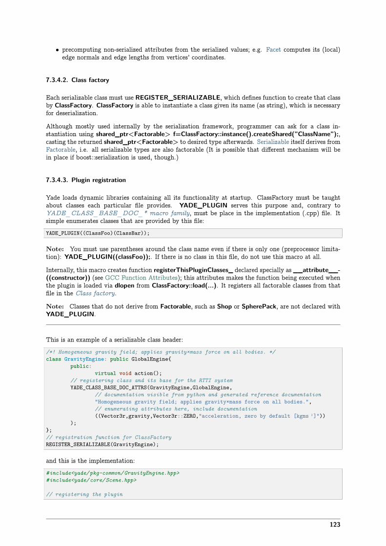
• precomputing non-serialized attributes from the serialized values; e.g. Facet computes its (local)edge normals and edge lengths from vertices’ coordinates.

7.3.4.2. Class factory

Each serializable class must use REGISTER_SERIALIZABLE, which defines function to create that classby ClassFactory. ClassFactory is able to instantiate a class given its name (as string), which is necessaryfor deserialization.

Although mostly used internally by the serialization framework, programmer can ask for a class in-stantiation using shared_ptr<Factorable> f=ClassFactory::instance().createShared(”ClassName”);,casting the returned shared_ptr<Factorable> to desired type afterwards. Serializable itself derives fromFactorable, i.e. all serializable types are also factorable (It is possible that different mechanism will bein place if boost::serialization is used, though.)

7.3.4.3. Plugin registration

Yade loads dynamic libraries containing all its functionality at startup. ClassFactory must be taughtabout classes each particular file provides. YADE_PLUGIN serves this purpose and, contrary toYADE_CLASS_BASE_DOC_* macro family, must be place in the implementation (.cpp) file. Itsimple enumerates classes that are provided by this file:

YADE_PLUGIN((ClassFoo)(ClassBar));

Note: You must use parentheses around the class name even if there is only one (preprocessor limita-tion): YADE_PLUGIN((classFoo));. If there is no class in this file, do not use this macro at all.

Internally, this macro creates function registerThisPluginClasses_ declared specially as __attribute__-((constructor)) (see GCC Function Attributes); this attributes makes the function being executed whenthe plugin is loaded via dlopen from ClassFactory::load(...). It registers all factorable classes from thatfile in the Class factory.

Note: Classes that do not derive from Factorable, such as Shop or SpherePack, are not declared withYADE_PLUGIN.

This is an example of a serializable class header:

/*! Homogeneous gravity field; applies gravity×mass force on all bodies. */class GravityEngine: public GlobalEngine{

public:virtual void action();

// registering class and its base for the RTTI systemYADE_CLASS_BASE_DOC_ATTRS(GravityEngine,GlobalEngine,

// documentation visible from python and generated reference documentation"Homogeneous gravity field; applies gravity×mass force on all bodies.",// enumerating attributes here, include documentation((Vector3r,gravity,Vector3r::ZERO,"acceleration, zero by default [kgms�²]"))

);};// registration function for ClassFactoryREGISTER_SERIALIZABLE(GravityEngine);

and this is the implementation:

#include<yade/pkg-common/GravityEngine.hpp>#include<yade/core/Scene.hpp>

// registering the plugin

123

YADE_PLUGIN((GravityEngine));

void GravityEngine::action(){/* do the work here */

}

We can create a mini-simulation (with only one GravityEngine):

Yade [67]: O.engines=[GravityEngine(gravity=Vector3(0,0,-9.81))]

Yade [68]: O.save('abc.xml')

and the XML looks like this:<Yade>

<scene _className_="Scene" tags="[author=V??clav~??milauer~(vaclav@flux) isoTime=20100531T100722 id=20100531T100722p5665 description=]" dt="1e-08" currentIteration="0" simulationTime="0" stopAtIteration="0" isPeriodic="0"><grpRelationData /><engines size="1">

<engines _className_="GravityEngine" label="" gravity="{0 0 -9.8100000000000005}" /></engines><initializers size="0" /><bodies _className_="BodyContainer" >

<body size="0" /></bodies><interactions _className_="InteractionContainer" serializeSorted="0">

<interaction size="0" /></interactions><materials size="0" /><miscParams size="0" /><dispParams size="0" /><cell _className_="Cell" refSize="{1 1 1}" trsf="{1 0 0 0 1 0 0 0 1}" velGrad="{0 0 0 0 0 0 0 0 0}" Hsize="{1 0 0 0 1 0 0 0 1}" />

</scene></Yade>

Warning: Since XML files closely reflect implementation details of Yade, they will not be compatiblebetween different versions. Use them only for short-term saving of scenes. Python is the high-leveldescription Yade uses.

7.3.4.4. Python attribute access

The macro YADE_CLASS_BASE_DOC_* macro family introduced above is (behind the scenes)also used to create functions for accessing attributes from Python. As already noted, set of serializedattributes and set of attributes accessible from Python are identical. Besides attribute access and the []operator access, these wrapper classes imitate also other functionality of regular python dictionaries:

Yade [69]: s=Sphere()

Yade [70]: s.radius ## read-access-> [70]: nan

Yade [71]: s.radius=4. ## write access

Yade [72]: s.keys() ## show all available keys-> [72]: ['radius', 'color', 'wire', 'highlight']

Yade [73]: for k in s.keys(): print s[k] ## iterate over keys, print their values....:

4.0Vector3(1,1,1)False

124

False

Yade [74]: s.has_key('radius') ## same as: 'radius' in s.keys()-> [74]: True

Yade [75]: s.dict() ## show dictionary of both attributes and values-> [75]: {'color': Vector3(1,1,1), 'highlight': False, 'radius': 4.0, 'wire': False}

## only very rarely needed; calls Serializable::postProcessAttributes(bool deserializing):Yade [77]: s.postProcessAttributes(False)

7.3.5. YADE_CLASS_BASE_DOC_* macro family

There is several macros that hide behind them the functionality of Sphinx documentation, Run-timetype identification (RTTI), Attribute registration, Python attribute access, plus automatic attributeinitialization and documentation. They are all defined as shorthands for base macro YADE_CLASS_-BASE_DOC_ATTRS_INIT_CTOR_PY with some arguments left out. They must be placed in classdeclaration’s body (.hpp file):

#define YADE_CLASS_BASE_DOC(klass,base,doc) \YADE_CLASS_BASE_DOC_ATTRS(klass,base,doc,)

#define YADE_CLASS_BASE_DOC_ATTRS(klass,base,doc,attrs) \YADE_CLASS_BASE_DOC_ATTRS_CTOR(klass,base,doc,attrs,)

#define YADE_CLASS_BASE_DOC_ATTRS_CTOR(klass,base,doc,attrs,ctor) \YADE_CLASS_BASE_DOC_ATTRS_CTOR_PY(klass,base,doc,attrs,ctor,)

#define YADE_CLASS_BASE_DOC_ATTRS_CTOR_PY(klass,base,doc,attrs,ctor,py) \YADE_CLASS_BASE_DOC_ATTRS_INIT_CTOR_PY(klass,base,doc,attrs,,ctor,py)

#define YADE_CLASS_BASE_DOC_ATTRS_INIT_CTOR_PY(klass,base,doc,attrs,init,ctor,py) \YADE_CLASS_BASE_DOC_ATTRS_DEPREC_INIT_CTOR_PY(klass,base,doc,attrs,,init,ctor,py)

Expected parameters are indicated by macro name components separated with underscores. Their mean-ing is as follows:

klass (unquoted) name of this class (used for RTTI and python)

base (unquoted) name of the base class (used for RTTI and python)

doc docstring of this class, written in the ReST syntax. This docstring will appear in generated docu-mentation (such as CpmMat). It can be as long as necessary, but sequences interpreted by c++compiler must be properly escaped (therefore some backslashes must be doubled, like in σ = ϵE:

":math:`\\sigma=\\epsilon E"

Use \n and \t for indentation inside the docstring. Hyperlink the documentation abundantly withyref (all references to other classes should be hyperlinks).

See Sphinx documentation for syntax details.

attrs Attribute must be written in the form of parethesized list:

((type1,attr1,initValue1,"Attribute 1 documentation"))((type2,attr2,,"Attribute 2 documentation")) // initValue unspecified

This will expand to

1. data members declaration in c++ (note that all attributes are public):

public: type1 attr1;type2 attr2;

125

2. Initializers of the default (argument-less) constructor, for attributes that have non-emptyinitValue:

Klass(): attr1(initValue1), attr2() { /* constructor body */ }

No initial value will be assigned for attribute of which initial value is left empty (asis for attr2 in the above example). Note that you still have to write the commas.

3. Registration of the attribute in the serialization system

4. Registration of the attribute in python, so that it can be accessed as klass().name1. Theattribute will be read-write; to avoid this, override it by read-only attribute of the samename in the py section (see below).

This attribute will carry the docstring provided, along with knowledge of the initial value.You can add text description to the default value using the comma operator of c++ andcasting the char* to (void):

((Real,dmgTau,((void)"deactivated if negative",-1),"Characteristic time for normal viscosity. [s]"))

leading to CpmMat::dmgTau.

The attribute is registered via boost::python::add_property specifying return_by_valuepolicy rather than return_internal_reference, which is the default when using def_-readwrite. The reason is that we need to honor custom converters for those values; seenote in Custom converters for details.

deprec List of deprecated attribute names. The syntax is

((oldName1,newName1,"Explanation why renamed etc."))((oldName2,newName2,"! Explanation why removed and what to do instaed."))

This will make accessing oldName1 attribute from Python return value of newName, but dis-playing warning message about the attribute name change, displaying provided explanation. Thishappens whether the access is read or write.

If the explanation’s first character is ! (bang), the message will be displayed upon attribute access,but exception will be thrown immediately. Use this in cases where attribute is no longer meaningfulor was not straightforwardsly replaced by another, but more complex adaptation of user’s script isneeded. You still have to give newName2, although its value will never be used – you can use anyvariable you like, but something must be given for syntax reasons).

Warning: Due to compiler limitations, this feature only works if Yade is compiled withgcc >= 4.4. In the contrary case, deprecated attribute functionality is disabled, even if suchattributes are declared.

init Parethesized list of the form:

((attr3,value3)) ((attr4,value4))

which will be expanded to initializers in the default ctor:

Klass(): /* attributes declared with the attrs argument */ attr4(value4), attr5(value5) { /* constructor body */ }

The purpose of this argument is to make it possible to initialize constants and references (whichare not declared as attributes using this macro themselves, but separately), as that cannot be donein constructor body. This argument is rarely used, though.

ctor will be put directly into the generated constructor’s body. Mostly used for calling createIndex(); inthe constructor.

126

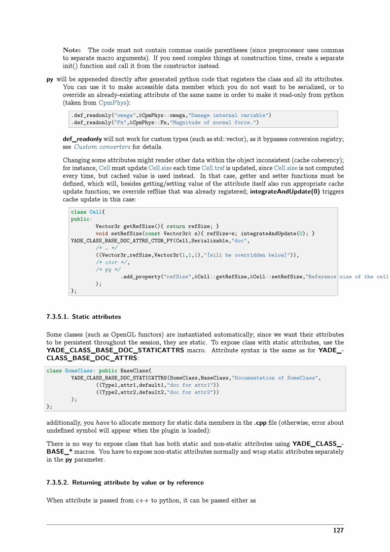
Note: The code must not contain commas ouside parentheses (since preprocessor uses commasto separate macro arguments). If you need complex things at construction time, create a separateinit() function and call it from the constructor instead.

py will be appeneded directly after generated python code that registers the class and all its attributes.You can use it to make accessible data member which you do not want to be serialized, or tooverride an already-existing attribute of the same name in order to make it read-only from python(taken from CpmPhys):

.def_readonly("omega",&CpmPhys::omega,"Damage internal variable")

.def_readonly("Fn",&CpmPhys::Fn,"Magnitude of normal force.")

def_readonly will not work for custom types (such as std::vector), as it bypasses conversion registry;see Custom converters for details.

Changing some attributes might render other data within the object inconsistent (cache coherency);for instance, Cell must update Cell.size each time Cell.trsf is updated, since Cell.size is not computedevery time, but cached value is used instead. In that case, getter and setter functions must bedefined, which will, besides getting/setting value of the attribute itself also run appropriate cacheupdate function; we override refSize that was already registered; integrateAndUpdate(0) triggerscache update in this case:

class Cell{public:

Vector3r getRefSize(){ return refSize; }void setRefSize(const Vector3r& s){ refSize=s; integrateAndUpdate(0); }

YADE_CLASS_BASE_DOC_ATTRS_CTOR_PY(Cell,Serializable,"doc",/* … */((Vector3r,refSize,Vector3r(1,1,1),"[will be overridden below]")),/* ctor */,/* py */

.add_property("refSize",&Cell::getRefSize,&Cell::setRefSize,"Reference size of the cell."));

};

7.3.5.1. Static attributes

Some classes (such as OpenGL functors) are instantiated automatically; since we want their attributesto be persistent throughout the session, they are static. To expose class with static attributes, use theYADE_CLASS_BASE_DOC_STATICATTRS macro. Attribute syntax is the same as for YADE_-CLASS_BASE_DOC_ATTRS:

class SomeClass: public BaseClass{YADE_CLASS_BASE_DOC_STATICATTRS(SomeClass,BaseClass,"Documentation of SomeClass",

((Type1,attr1,default1,"doc for attr1"))((Type2,attr2,default2,"doc for attr2"))

);};

additionally, you have to allocate memory for static data members in the .cpp file (otherwise, error aboutundefined symbol will appear when the plugin is loaded):

There is no way to expose class that has both static and non-static attributes using YADE_CLASS_-BASE_*macros. You have to expose non-static attributes normally and wrap static attributes separatelyin the py parameter.

7.3.5.2. Returning attribute by value or by reference

When attribute is passed from c++ to python, it can be passed either as

127

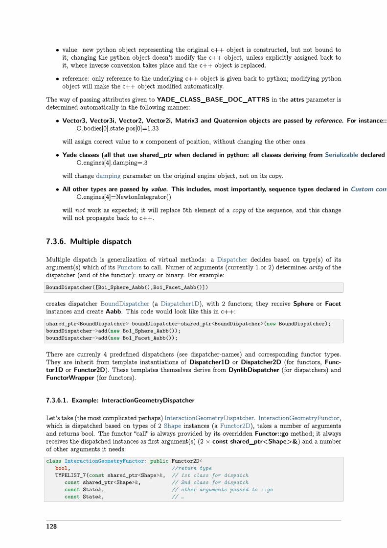
• value: new python object representing the original c++ object is constructed, but not bound toit; changing the python object doesn’t modify the c++ object, unless explicitly assigned back toit, where inverse conversion takes place and the c++ object is replaced.

• reference: only reference to the underlying c++ object is given back to python; modifying pythonobject will make the c++ object modified automatically.

The way of passing attributes given to YADE_CLASS_BASE_DOC_ATTRS in the attrs parameter isdetermined automatically in the following manner:

• Vector3, Vector3i, Vector2, Vector2i, Matrix3 and Quaternion objects are passed by reference. For instance::O.bodies[0].state.pos[0]=1.33

will assign correct value to x component of position, without changing the other ones.

• Yade classes (all that use shared_ptr when declared in python: all classes deriving from Serializable declared with YADE_CLASS_BASE_DOC_*, and some others) are passed as references (technically speaking, they are passed by value of the shared_ptr, but by virtue of its sharedness, they appear as references). For instance::O.engines[4].damping=.3

will change damping parameter on the original engine object, not on its copy.

• All other types are passed by value. This includes, most importantly, sequence types declared in Custom converters, such as std::vector<shared_ptr<Engine> >. For this reason, ::O.engines[4]=NewtonIntegrator()

will not work as expected; it will replace 5th element of a copy of the sequence, and this changewill not propagate back to c++.

7.3.6. Multiple dispatch

Multiple dispatch is generalization of virtual methods: a Dispatcher decides based on type(s) of itsargument(s) which of its Functors to call. Numer of arguments (currently 1 or 2) determines arity of thedispatcher (and of the functor): unary or binary. For example:BoundDispatcher([Bo1_Sphere_Aabb(),Bo1_Facet_Aabb()])

creates dispatcher BoundDispatcher (a Dispatcher1D), with 2 functors; they receive Sphere or Facetinstances and create Aabb. This code would look like this in c++:shared_ptr<BoundDispatcher> boundDispatcher=shared_ptr<BoundDispatcher>(new BoundDispatcher);boundDispatcher->add(new Bo1_Sphere_Aabb());boundDispatcher->add(new Bo1_Facet_Aabb());

There are currenly 4 predefined dispatchers (see dispatcher-names) and corresponding functor types.They are inherit from template instantiations of Dispatcher1D or Dispatcher2D (for functors, Func-tor1D or Functor2D). These templates themselves derive from DynlibDispatcher (for dispatchers) andFunctorWrapper (for functors).

7.3.6.1. Example: InteractionGeometryDispatcher

Let’s take (the most complicated perhaps) InteractionGeometryDispatcher. InteractionGeometryFunctor,which is dispatched based on types of 2 Shape instances (a Functor2D), takes a number of argumentsand returns bool. The functor “call” is always provided by its overridden Functor::go method; it alwaysreceives the dispatched instances as first argument(s) (2 × const shared_ptr<Shape>&) and a numberof other arguments it needs:class InteractionGeometryFunctor: public Functor2D<

bool, //return typeTYPELIST_7(const shared_ptr<Shape>&, // 1st class for dispatch

const shared_ptr<Shape>&, // 2nd class for dispatchconst State&, // other arguments passed to ::goconst State&, // …

128

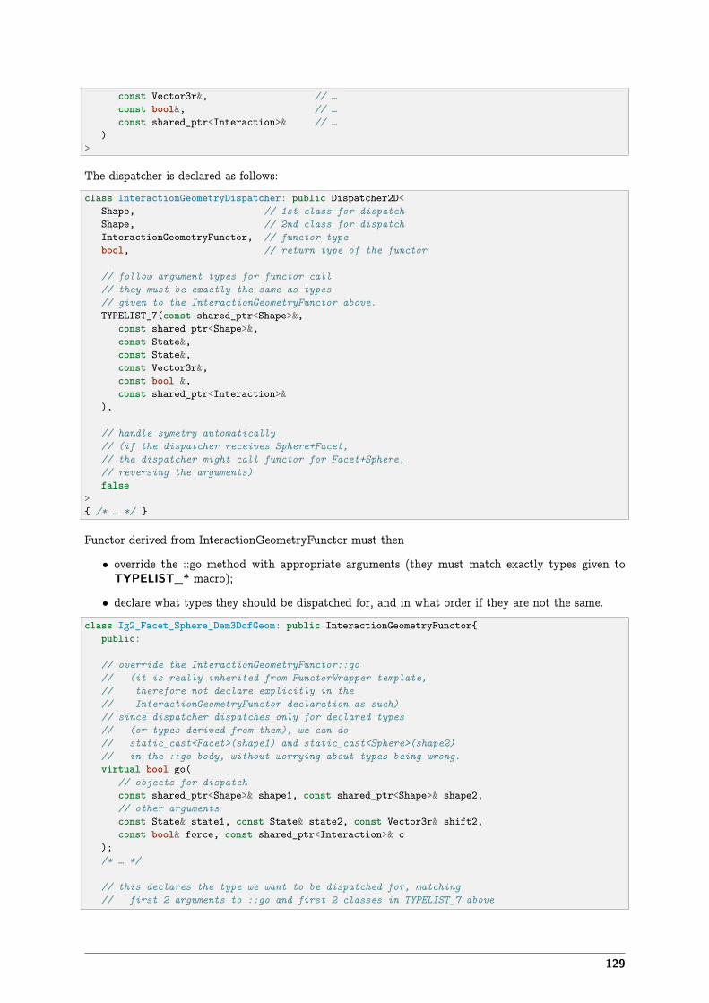
const Vector3r&, // …const bool&, // …const shared_ptr<Interaction>& // …

)>

The dispatcher is declared as follows:class InteractionGeometryDispatcher: public Dispatcher2D<

Shape, // 1st class for dispatchShape, // 2nd class for dispatchInteractionGeometryFunctor, // functor typebool, // return type of the functor

// follow argument types for functor call// they must be exactly the same as types// given to the InteractionGeometryFunctor above.TYPELIST_7(const shared_ptr<Shape>&,

const shared_ptr<Shape>&,const State&,const State&,const Vector3r&,const bool &,const shared_ptr<Interaction>&

),

// handle symetry automatically// (if the dispatcher receives Sphere+Facet,// the dispatcher might call functor for Facet+Sphere,// reversing the arguments)false

>{ /* … */ }

Functor derived from InteractionGeometryFunctor must then

• override the ::go method with appropriate arguments (they must match exactly types given toTYPELIST_* macro);

• declare what types they should be dispatched for, and in what order if they are not the same.

class Ig2_Facet_Sphere_Dem3DofGeom: public InteractionGeometryFunctor{public:

// override the InteractionGeometryFunctor::go// (it is really inherited from FunctorWrapper template,// therefore not declare explicitly in the// InteractionGeometryFunctor declaration as such)// since dispatcher dispatches only for declared types// (or types derived from them), we can do// static_cast<Facet>(shape1) and static_cast<Sphere>(shape2)// in the ::go body, without worrying about types being wrong.virtual bool go(

// objects for dispatchconst shared_ptr<Shape>& shape1, const shared_ptr<Shape>& shape2,// other argumentsconst State& state1, const State& state2, const Vector3r& shift2,const bool& force, const shared_ptr<Interaction>& c

);/* … */

// this declares the type we want to be dispatched for, matching// first 2 arguments to ::go and first 2 classes in TYPELIST_7 above

129

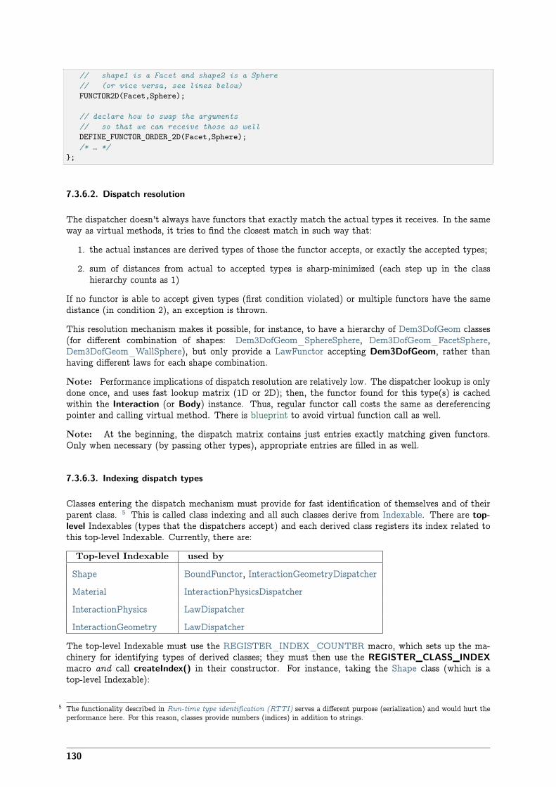
// shape1 is a Facet and shape2 is a Sphere// (or vice versa, see lines below)FUNCTOR2D(Facet,Sphere);

// declare how to swap the arguments// so that we can receive those as wellDEFINE_FUNCTOR_ORDER_2D(Facet,Sphere);/* … */

};

7.3.6.2. Dispatch resolution

The dispatcher doesn’t always have functors that exactly match the actual types it receives. In the sameway as virtual methods, it tries to find the closest match in such way that:

1. the actual instances are derived types of those the functor accepts, or exactly the accepted types;

2. sum of distances from actual to accepted types is sharp-minimized (each step up in the classhierarchy counts as 1)

If no functor is able to accept given types (first condition violated) or multiple functors have the samedistance (in condition 2), an exception is thrown.

This resolution mechanism makes it possible, for instance, to have a hierarchy of Dem3DofGeom classes(for different combination of shapes: Dem3DofGeom_SphereSphere, Dem3DofGeom_FacetSphere,Dem3DofGeom_WallSphere), but only provide a LawFunctor accepting Dem3DofGeom, rather thanhaving different laws for each shape combination.

Note: Performance implications of dispatch resolution are relatively low. The dispatcher lookup is onlydone once, and uses fast lookup matrix (1D or 2D); then, the functor found for this type(s) is cachedwithin the Interaction (or Body) instance. Thus, regular functor call costs the same as dereferencingpointer and calling virtual method. There is blueprint to avoid virtual function call as well.

Note: At the beginning, the dispatch matrix contains just entries exactly matching given functors.Only when necessary (by passing other types), appropriate entries are filled in as well.

7.3.6.3. Indexing dispatch types

Classes entering the dispatch mechanism must provide for fast identification of themselves and of theirparent class. 5 This is called class indexing and all such classes derive from Indexable. There are top-level Indexables (types that the dispatchers accept) and each derived class registers its index related tothis top-level Indexable. Currently, there are:

Top-level Indexable used by

Shape BoundFunctor, InteractionGeometryDispatcher

Material InteractionPhysicsDispatcher

InteractionPhysics LawDispatcher

InteractionGeometry LawDispatcher

The top-level Indexable must use the REGISTER_INDEX_COUNTER macro, which sets up the ma-chinery for identifying types of derived classes; they must then use the REGISTER_CLASS_INDEXmacro and call createIndex() in their constructor. For instance, taking the Shape class (which is atop-level Indexable):

5 The functionality described in Run-time type identification (RTTI) serves a different purpose (serialization) and would hurt theperformance here. For this reason, classes provide numbers (indices) in addition to strings.

130

// derive from Indexableclass Shape: public Serializable, public Indexable {

// never call createIndex() in the top-level Indexable ctor!/* … */

// allow index registration for classes deriving from ``Shape``REGISTER_INDEX_COUNTER(Shape);

};

Now, all derived classes (such as Sphere or Facet) use this:

class Sphere: public Shape{/* … */YADE_CLASS_BASE_DOC_ATTRS_CTOR(Sphere,Shape,"docstring",

((Type1,attr1,default1,"docstring1"))/* … */,// this is the CTOR argument

// important; assigns index to the class at runtimecreateIndex();

);// register index for this class, and give name of the immediate parent class// (i.e. if there were a class deriving from Sphere, it would use// REGISTER_CLASS_INDEX(SpecialSphere,Sphere),// not REGISTER_CLASS_INDEX(SpecialSphere,Shape)!)REGISTER_CLASS_INDEX(Sphere,Shape);

};

At runtime, each class within the top-level Indexable hierarchy has its own unique numerical index.These indices serve to build the dispatch matrix for each dispatcher.

7.3.6.4. Inspecting dispatch in python

If there is a need to debug/study multiple dispatch, python provides convenient interface for this low-levelfunctionality.

We can inspect indices with the dispIndex property (note that the top-level indexable Shape has negative(invalid) class index; we purposively didn’t call createIndex in its constructor):

Yade [78]: Sphere().dispIndex, Facet().dispIndex, Wall().dispIndex-> [78]: (2, 1, 4)

Yade [79]: Shape().dispIndex # top-level indexable-> [79]: -1

Dispatch hierarchy for a particular class can be shown with the dispHierarchy() function, returning listof class names: 0th element is the instance itself, last element is the top-level indexable (again, withinvalid index); for instance:

Yade [80]: Dem3DofGeom().dispHierarchy() # parent class of all other Dem3DofGeom_ classes-> [80]: ['Dem3DofGeom', 'InteractionGeometry']

Yade [81]: Dem3DofGeom_SphereSphere().dispHierarchy(), Dem3DofGeom_FacetSphere().dispHierarchy(), Dem3DofGeom_WallSphere().dispHierarchy()-> [81]:(['Dem3DofGeom_SphereSphere', 'Dem3DofGeom', 'InteractionGeometry'],['Dem3DofGeom_FacetSphere', 'Dem3DofGeom', 'InteractionGeometry'],['Dem3DofGeom_WallSphere', 'Dem3DofGeom', 'InteractionGeometry'])

Yade [82]: Dem3DofGeom_WallSphere().dispHierarchy(names=False) # show numeric indices instead-> [82]: [4, 1, -1]

Dispatchers can also be inspected, using the .dispMatrix() method:

131

Yade [83]: ig=InteractionGeometryDispatcher([....: Ig2_Sphere_Sphere_Dem3DofGeom(),....: Ig2_Facet_Sphere_Dem3DofGeom(),....: Ig2_Wall_Sphere_Dem3DofGeom()....: ])

Yade [88]: ig.dispMatrix()-> [88]:{('Facet', 'Sphere'): 'Ig2_Facet_Sphere_Dem3DofGeom',('Sphere', 'Facet'): 'Ig2_Facet_Sphere_Dem3DofGeom',('Sphere', 'Sphere'): 'Ig2_Sphere_Sphere_Dem3DofGeom',('Sphere', 'Wall'): 'Ig2_Wall_Sphere_Dem3DofGeom',('Wall', 'Sphere'): 'Ig2_Wall_Sphere_Dem3DofGeom'}

Yade [89]: ig.dispMatrix(False) # don't convert to class names-> [89]:{(1, 2): 'Ig2_Facet_Sphere_Dem3DofGeom',(2, 1): 'Ig2_Facet_Sphere_Dem3DofGeom',(2, 2): 'Ig2_Sphere_Sphere_Dem3DofGeom',(2, 4): 'Ig2_Wall_Sphere_Dem3DofGeom',(4, 2): 'Ig2_Wall_Sphere_Dem3DofGeom'}

We can see that functors make use of symmetry (i.e. that Sphere+Wall are dispatched to the samefunctor as Wall+Sphere).

Finally, dispatcher can be asked to return functor suitable for given argument(s):

Yade [90]: ld=LawDispatcher([Law2_Dem3DofGeom_CpmPhys_Cpm()])

Yade [91]: ld.dispMatrix()-> [91]: {('Dem3DofGeom', 'CpmPhys'): 'Law2_Dem3DofGeom_CpmPhys_Cpm'}

# see how the entry for Dem3DofGeom_SphereSphere will be filled after this requestYade [93]: ld.dispFunctor(Dem3DofGeom_SphereSphere(),CpmPhys())-> [93]: <Law2_Dem3DofGeom_CpmPhys_Cpm instance at 0x2cc8170>

Yade [94]: ld.dispMatrix()-> [94]:{('Dem3DofGeom', 'CpmPhys'): 'Law2_Dem3DofGeom_CpmPhys_Cpm',('Dem3DofGeom_SphereSphere', 'CpmPhys'): 'Law2_Dem3DofGeom_CpmPhys_Cpm'}

7.3.6.5. OpenGL functors

OpenGL rendering is being done also by 1D functors (dispatched for the type to be rendered). Since itis sufficient to have exactly one class for each rendered type, the functors are found automatically. Theirbase functor types are GlShapeFunctor, GlBoundFunctor, GlInteractionGeometryFunctor and so on.These classes register the type they render using the RENDERS macro:

class Gl1_Sphere: public GlShapeFunctor {public :

virtual void go(const shared_ptr<Shape>&,const shared_ptr<State>&,bool wire,const GLViewInfo&

);RENDERS(Sphere);YADE_CLASS_BASE_DOC_STATICATTRS(Gl1_Sphere,GlShapeFunctor,"docstring",

((Type1,staticAttr1,informativeDefault,"docstring"))/* … */

);};

132

REGISTER_SERIALIZABLE(Gl1_Sphere);

You can list available functors of a particular type by querying child classes of the base functor:

Yade [96]: yade.system.childClasses('GlShapeFunctor')-> [96]: set(['Gl1_Box', 'Gl1_Facet', 'Gl1_Sphere', 'Gl1_Tetra', 'Gl1_Wall'])

Note: OpenGL functors may disappear in the future, being replaced by virtual functions of each classthat can be rendered.

7.3.7. Parallel execution

Yade was originally not designed with parallel computation in mind, but rather with maximum flexibility(for good or for bad). Parallel execution was added later; in order to not have to rewrite whole Yadefrom scratch, relatively non-instrusive way of parallelizing was used: [OpenMP]. OpenMP is standartizedshared-memory parallel execution environment, where parallel sections are marked by special #pragmain the code (which means that they can compile with compiler that doesn’t support OpenMP) and a fewfunctions to query/manipulate OpenMP runtime if necessary.

There is parallelism at 3 levels:

• Computation, interaction (python, GUI) and rendering threads are separate. This is done viaregular threads (boost::threads) and is not related to OpenMP.

• ParallelEngine can run multiple engine groups (which are themselves run serially) in parallel; itrarely finds use in regular simulations, but it could be used for example when coupling with anindependent expensive computation:

ParallelEngine([[Engine1(),Engine2()], # Engine1 will run before Engine2[Engine3()] # Engine3() will run in parallel with the group [Engine1(),Engine2()]

# arbitrary number of groups can be used])

Engine2 will be run after Engine1, but in parallel with Engine3.

Warning: It is your reponsibility to avoid concurrent access to data when usingParallelEngine. Make sure you understand very well what the engines run in paralleldo.

• Parallelism inside Engines. Some loops over bodies or interactions are parallelized (notably Inter-actionDispatchers and NewtonIntegrator, which are treated in detail later (FIXME: link)):

#pragma omp parallel forfor(long id=0; id<size; id++){

const shared_ptr<Body>& b(scene->bodies[id]);/* … */

}

Note: OpenMP requires loops over contiguous range of integers (OpenMP 3 also acceptscontainers with random-access iterators).

If you consider running parallelized loop in your engine, always evalue its benefits.OpenMP has some overhead fo creating threads and distributing workload, which isproportionally more expensive if the loop body execution is fast. The results are highlyhardware-dependent (CPU caches, RAM controller).

Maximum number of OpenMP threads is determined by the OMP_NUM_THREADS environmentvariable and is constant throughout the program run. Yade main program also sets this variable (beforeloading OpenMP libraries) if you use the -j/--threads option. It can be queried at runtime with the

133

omp_get_max_threads function.

At places which are susceptible of being accessed concurrently from multiple threads, Yade provides somemutual exclusion mechanisms, discussed elsewhere (FIXME):

• simultaneously writeable container for ForceContainer,

• mutex for Body::State.

7.3.8. Logging

Regardless of whether the optional-libraries log4cxx is used or not, yade provides logging macros. 6 Iflog4cxx is enabled, these macros internally operate on the local logger instance (named logger, but thatis hidden for the user); if log4cxx is disabled, they send their arguments to standard error output (cerr).

Every class using logging should create logger using these 2 macros (they expand to nothing if log4cxxis not used):

DECLARE_LOGGER; in class declaration body (in the .hpp file); this declares static variable logger;

CREATE_LOGGER(ClassName); in the implementation file; it creates and initializes that static vari-able. The logger will be named yade.ClassName.

The logging macros are the following:

• LOG_TRACE, LOG_DEBUG, LOG_INFO, LOG_WARN, LOG_ERROR, LOG_FATAL (in-creasing severity); their argument is fed to the logger stream, hence can contain the << operation:

LOG_WARN("Exceeded "<<maxSteps<<" steps in attempts to converge, the result returned will not be precise (relative error "<<relErr<<", tolerance "<<relTol<<")");

Every log message is prepended filename, line number and function name; the final mes-sage that will appear will look like this:

237763 WARN yade.ViscosityIterSolver /tmp/yade/trunk/extra/ViscosityIterSolver.cpp:316 newtonRaphsonSolve: Exceeded 30 steps in attempts to converge, the result returned will not be precise (relative error 5.2e-3, tolerance 1e-3)

The 237763 WARN yade.ViscosityIterSolver (microseconds from start, severity, loggername) is added by log4cxx and is completely configurable, either programatically, or byusing file ~/.yade-$SUFFIX/logging.conf, which is loaded at startup, if present (FIXME:see more etc user’s guide)

• special tracing macros TRVAR1, TRVAR2, … TRVAR6, which show both variable name andits value (there are several more macros defined inside /lib/base/Logging.hpp, but they are notgenerally in use):

TRVAR3(var1,var2,var3);// will be expanded to:LOG_TRACE("var1="<<var1<<"; var2="<<var2<<"; var3="<<var3);

Note: For performance reasons, optimized builds eliminate LOG_TRACE and LOG_DEBUG from thecode at preprocessor level.

Note: Builds without log4cxx (even in debug mode) eliminate LOG_TRACE and LOG_DEBUG. Asthere is no way to enable/disable them selectively, the log amount would be huge.

Python provides rudimentary control for the logging system in yade.log module (FIXME: ref to docs):

Yade [97]: from yade import log

Yade [98]: log.setLevel('InsertionSortCollider',log.DEBUG) # sets logging level of the yade.InsertionSortCollider logger

6 Because of (seemingly?) no upstream development of log4cxx and a few problems it has, Yade will very likely move to thehypothetical boost::logging library once it exists. The logging code will not have to be changed, however, as the log4cxx logic ishidden behind these macros.

134

Yade [99]: log.setLevel('',log.WARN) # sets logging level of all yade.* loggers (they inherit level from the parent logger, except when overridden)

As of now, there is no python interface for performing logging into lo4cxx loggers themselves.

7.3.9. Timing

Yade provides 2 services for measuring time spent in different pars of the code. One has the granularityof engine and can be enabled at runtime. The other one is finer, but requires adjusting and recompilingthe code being measured.

7.3.9.1. Per-engine timing

The coarser timing works by merely accumulating numebr of invocations and time (with the precisionof the clock_gettime function) spent in each engine, which can be then post-processed by associatedPython module yade.timing. There is a static bool variable controlling whether such measurements takeplace (disabled by default), which you can change

TimingInfo::enabled=True; // in c++

O.timingEnabled=True ## in python

After running the simulation, yade.timing.stats() function will show table with the results and percent-ages:

Yade [100]: TriaxialTest(numberOfGrains=100).load()

Yade [101]: O.engines[0].label='firstEngine' ## labeled engines will show by labels in the stats table

Yade [102]: import yade.timing;Yade [103]: O.timingEnabled=True

Yade [104]: yade.timing.reset() ## not necessary if used for the first time

Yade [105]: O.run(50); O.wait()

Yade [106]: yade.timing.stats()Name Count Time Rel. time-------------------------------------------------------------------------------------------------------"firstEngine" 50 63us 0.19%BoundDispatcher 2 23us 0.07%InsertionSortCollider 50 2245us 6.67%InteractionDispatchers 50 1313us 3.90%GlobalStiffnessTimeStepper 2 25us 0.08%TriaxialCompressionEngine 50 367us 1.09%TriaxialStateRecorder 3 29161us 86.61%NewtonIntegrator 50 470us 1.40%TOTAL 33669us 100.00%

Exec count and time can be accessed and manipulated through Engine::timingInfo from c++ or En-gine().execCount and Engine().execTime properties in Python.

7.3.9.2. In-engine and in-functor timing

Timing within engines (and functors) is based on TimingDeltas class. It is made for timing loops (func-tors’ loop is in their respective dispatcher) and stores cummulatively time differences between check-points.

135

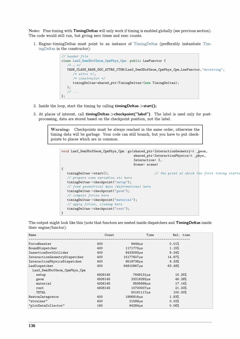
Note: Fine timing with TimingDeltas will only work if timing is enabled globally (see previous section).The code would still run, but giving zero times and exec counts.

1. Engine::timingDeltas must point to an instance of TimingDeltas (prefferably instantiate Tim-ingDeltas in the constructor):

// header fileclass Law2_Dem3DofGeom_CpmPhys_Cpm: public LawFunctor {

/* … */YADE_CLASS_BASE_DOC_ATTRS_CTOR(Law2_Dem3DofGeom_CpmPhys_Cpm,LawFunctor,"docstring",

/* attrs */,/* constructor */timingDeltas=shared_ptr<TimingDeltas>(new TimingDeltas);

);// ...

};

2. Inside the loop, start the timing by calling timingDeltas->start();

3. At places of interest, call timingDeltas->checkpoint(”label”). The label is used only for post-processing, data are stored based on the checkpoint position, not the label.

Warning: Checkpoints must be always reached in the same order, otherwise thetiming data will be garbage. Your code can still branch, but you have to put check-points to places which are in common.

void Law2_Dem3DofGeom_CpmPhys_Cpm::go(shared_ptr<InteractionGeometry>& _geom,shared_ptr<InteractionPhysics>& _phys,Interaction* I,Scene* scene)

{timingDeltas->start(); // the point at which the first timing starts// prepare some variables etc heretimingDeltas->checkpoint("setup");// find geometrical data (deformations) heretimingDeltas->checkpoint("geom");// compute forces heretimingDeltas->checkpoint("material");// apply forces, cleanup heretimingDeltas->checkpoint("rest");

}

The output might look like this (note that functors are nested inside dispatchers and TimingDeltas insidetheir engine/functor):Name Count Time Rel. time-------------------------------------------------------------------------------------ForceReseter 400 9449µs 0.01%BoundDispatcher 400 1171770µs 1.15%InsertionSortCollider 400 9433093µs 9.24%InteractionGeometryDispatcher 400 15177607µs 14.87%InteractionPhysicsDispatcher 400 9518738µs 9.33%LawDispatcher 400 64810867µs 63.49%Law2_Dem3DofGeom_CpmPhys_Cpm

setup 4926145 7649131µs 15.25%geom 4926145 23216292µs 46.28%material 4926145 8595686µs 17.14%rest 4926145 10700007µs 21.33%TOTAL 50161117µs 100.00%

NewtonIntegrator 400 1866816µs 1.83%"strainer" 400 21589µs 0.02%"plotDataCollector" 160 64284µs 0.06%

136

"damageChecker" 9 3272µs 0.00%TOTAL 102077490µs 100.00%

Warning: Do not use TimingDeltas in parallel sections, results might not be meaningful. Inparticular, avoid timing functors inside InteractionDispatchers when running with multiple OpenMPthreads.

TimingDeltas data are accessible from Python as list of (label,*time*,*count*) tuples, one tuple repre-senting each checkpoint:

deltas=someEngineOrFunctor.timingDeltas.data()deltas[0][0] # 0th checkpoint labeldeltas[0][1] # 0th checkpoint time in nanosecondsdeltas[0][2] # 0th checkpoint execution countdeltas[1][0] # 1st checkpoint label

# …deltas.reset()

7.3.9.3. Timing overhead

The overhead of the coarser, per-engine timing, is very small. For simulations with at least severalhundreds of elements, they are below the usual time variance (a few percent).

The finer TimingDeltas timing can have major performance impact and should be only used duringdebugging and performance-tuning phase. The parts that are file-timed will take disproportionally longertime that the rest of engine; in the output presented above, LawDispatcher takes almost � of totalsimulation time in average, but the number would be twice of thrice lower typically (note that eachcheckpoint was timed almost 5 million times in this particular case).

7.3.10. OpenGL Rendering

Yade provides 3d rendering based on [QGLViewer]. It is not meant to be full-featured rendering andpost-processing, but rather a way to quickly check that scene is as intended or that simulation behavessanely.

Note: Although 3d rendering runs in a separate thread, it has performance impact on the computa-tion itself, since interaction container requires mutual exclusion for interaction creation/deletion. TheInteractionContainer::drawloopmutex is either held by the renderer (OpenGLRenderingEngine) or bythe insertion/deletion routine.

Warning: There are 2 possible causes of crash, which are not prevented because of serious perfor-mance penalty that would result:

1. access to BodyContainer, in particular deleting bodies from simulation; this is a rare operation,though.

2. deleting Interaction::interactionPhysics or Interaction::interactionGeometry.

Renderable entities (Shape, State, Bound, InteractionGeometry, InteractionPhysics) have their associatedOpenGL functors. An entity is rendered if

1. Rendering such entities is enabled by appropriate attribute in OpenGLRenderingEngine

2. Functor for that particular entity type is found via the dispatch mechanism.

Gl1_* functors operating on Body’s attributes (Shape, State, Bound) are called with the OpenGLcontext translated and rotated according to State::pos and State::ori. Interaction functors work in globalcoordinates.

137

7.4. Simulation framework

Besides the support framework mentioned in the previous section, some functionality pertaining to sim-ulation itself is also provided.

There are special containers for storing bodies, interactions and (generalized) forces. Their internal func-tioning is normally opaque to the programmer, but should be understood as it can influence performance.

7.4.1. Scene

Scene is the object containing the whole simulation. Although multiple scenes can be present in thememory, only one of them is active. Saving and loading (serializing and deserializing) the Scene objectshould make the simulation run from the point where it left off.

Note: All Engines and functors have interally a Scene* scene pointer which is updated regularly byengine/functor callers; this ensures that the current scene can be accessed from within user code.

For outside functions (such as those called from python, or static functions in Shop), you can useOmega::instance().getScene() to retrieve a shared_ptr<Scene> of the current scene.

7.4.2. Body container

Body container is linear storage of bodies. Each body in the simulation has its unique id, under which itmust be found in the BodyContainer. Body that is not yet part of the simulation typically has id equalto invalid value Body::ID_NONE, and will have its id assigned upon insertion into the container. Therequirements on BodyContainer are

• O(1) access to elements,

• linear-addressability (0…n indexability),

• store shared_ptr, not objects themselves,

• no mutual exclusion for insertion/removal (this must be assured by the called, if desired),

• intelligent allocation of id for new bodies (tracking removed bodies),

• easy iteration over all bodies.

Note: Currently, there is “abstract” class BodyContainer, from which derive concrete implementations;the initial idea was the ability to select at runtime which implementation to use (to find one that performsthe best for given simulation). This incurs the penalty of many virtual function calls, and will probablychange in the future. All implementations of BodyContainer were removed in the meantime, exceptBodyVector (internally a vector<shared_ptr<Body> > plus a few methods around), which is thefastest.

7.4.2.1. Insertion/deletion

Body insertion is typically used in FileGenerator‘s:

shared_ptr<Body> body(new Body);// … (body setup)scene->bodies->insert(body); // assigns the id

Bodies are deleted only rarely:

138

scene->bodies->erase(id);

Warning: Since mutual exclusion is not assured, never insert/erase bodies from parallel sections,unless you explicitly assure there will be no concurrent access.

7.4.2.2. Iteration

The container can be iterated over using FOREACH macro (shorthand for BOOST_FOREACH):

FOREACH(const shared_ptr<Body>& b, *scene->bodies){if(!b) continue; // skip deleted bodies/* do something here */

}

Note a few important things:

1. Always use const shared_ptr<Body>& (const reference); that avoids incrementing and decre-menting the reference count on each shared_ptr.

2. Take care to skip NULL bodies (if(!b) continue): deleted bodies are deallocated from the container,but since body id’s must be persistent, their place is simply held by an empty shared_ptr<Body>()object, which is implicitly convertible to false.

In python, the BodyContainer wrapper also has iteration capabilities; for convenience (which is differentfrom the c++ iterator), NULL bodies as silently skipped:

Yade [108]: O.bodies.append([Body(),Body(),Body()])-> [108]: [0, 1, 2]

Yade [109]: O.bodies.erase(1)-> [109]: True

Yade [110]: [b.id for b in O.bodies]-> [110]: [0, 2]

In loops parallelized using OpenMP, the loop must traverse integer interval (rather than using iterators):

const long size=(long)bodies.size(); // store this value, since it doesn't change during the loop#pragma omp parallel forfor(long _id=0; _id<size; _id++){

const shared_ptr<Body>& b(bodies[_id]);if(!b) continue;/* … */

}

7.4.3. InteractionContainer

Interactions are stored in special container, and each interaction must be uniquely identified by pair ofids (id1,id2).

• O(1) access to elements,

• linear-addressability (0…n indexability),

• store shared_ptr, not objects themselves,

• mutual exclusion for insertion/removal,

• easy iteration over all interactions,

139

• addressing symmetry, i.e. interaction(id1,id2)�interaction(id2,id1)

Note: As with BodyContainer, there is “abstract” class InteractionContainer, and then its concreteimplementations. Currently, only InteractionVecMap implementation is used and all the other wereremoved. Therefore, the abstract InteractionContainer class may disappear in the future, to avoid un-necessary virtual calls.

Further, there is a blueprint for storing interactions inside bodies, as that would give extra advantage ofquickly getting all interactions of one particular body (currently, this necessitates loop over all interac-tions); in that case, InteractionContainer would disappear.

7.4.3.1. Insert/erase

Creating new interactions and deleting them is delicate topic, since many eleents of simulation must besynchronized; the exact workflow is described in Handling interactions. You will almost certainly neverneed to insert/delete an interaction manually from the container; if you do, consider designing your codedifferently.

// both insertion and erase are internally protected by a mutex,// and can be done from parallel sections safelyscene->interactions->insert(shared_ptr<Interaction>(new Interactions(id1,id2)));scene->interactions->erase(id1,id2);

7.4.3.2. Iteration

As with BodyContainer, iteration over interactions should use the FOREACH macro:

FOREACH(const shared_ptr<Interaction>& i, *scene->interactions){if(!i->isReal()) continue;/* … */

}

Again, note the usage const reference for i. The check if(!i->isReal()) filters away interactions that existonly potentially, i.e. there is only Bound overlap of the two bodies, but not (yet) overlap of bodies them-selves. The i->isReal() function is equivalent to i->interactionGeometry && i->interactionPhysics.Details are again explained in Handling interactions.

In some cases, such as OpenMP-loops requiring integral index (OpenMP >= 3.0 allows parallelizationusing random-access iterator as well), you need to iterate over interaction indices instead:

inr nIntr=(int)scene->interactions->size(); // hoist container size#pragma omp parallel forfor(int j=0; j<nIntr, j++){

const shared_ptr<Interaction>& i(scene->interactions[j]);if(!->isReal()) continue;/* … */

}

7.4.4. ForceContainer

ForceContainer holds “generalized forces”, i.e. forces, torques, (explicit) dispalcements and rotations foreach body.

During each computation step, there are typically 3 phases pertaining to forces:

1. Resetting forces to zero (usually done by the ForceResetter engine)

2. Incrementing forces from parallel sections (solving interactions – from LawFunctor)

140

3. Reading absolute force values sequentially for each body: forces applied from different interactionsare summed together to give overall force applied on that body (NewtonIntegrator, but also variousother engine that read forces)

This scenario leads to special design, which allows fast parallel write access:

• each thread has its own storage (zeroed upon request), and only write to its own storage; this avoidsconcurrency issues. Each thread identifies itself by the omp_get_thread_num() function providedby the OpenMP runtime.

• before reading absolute values, the container must be synchronized, i.e. values from all threadsare summed up and stored separately. This is a relatively slow operation and we provide Force-Container::syncCount that you might check to find cummulative number of synchronizations andcompare it agains number of steps. Ideally, ForceContainer is only synchronized once at each step.

• the container is resized whenever an element outside the current range is read/written to (theread returns zero in that case); this avoids the necessity of tracking number of bodies, but alsois potential danger (such as scene->forces.getForce(1000000000), which will probably exhaustyour RAM). Unlike c++, Python does check given id against number of bodies.

// resetting forces (inside ForceResetter)scene->forces.reset()

// in a parallel sectionscene->forces.addForce(id,force); // add force

// container is not synced after we wrote to it, sync before readingscene->forces.sync();const Vector3r& f=scene->forces.getForce(id);

Synchronization is handled automatically if values are read from python:Yade [111]: O.bodies.append(Body())-> [111]: 1

Yade [112]: O.forces.addF(0,Vector3(1,2,3))

Yade [113]: O.forces.f(0)-> [113]: Vector3(1,2,3)

Yade [114]: O.forces.f(100)---------------------------------------------------------------------------IndexError Traceback (most recent call last)

/home/vaclav/ydoc/<ipython console> in <module>()

IndexError: Body id out of range.

7.4.5. Handling interactions

Creating and removing interactions is a rather delicate topic and number of components must cooperateso that the whole behaves as expected.

Terminologically, we distinguish

potential interactions, having neither geometry nor physics. Interaction.real can be used to query thestatus (Interaction::isReal() in c++).

real interactions, having both geometry and physics. Below, we shall discuss the possibility of interac-tions that only have geometry but no physics.

During each step in the simulation, the following operations are performed on interactions in a typical

141

simulation:

1. Collider creates potential interactions based on spatial proximity. Not all pairs of bodies are sus-ceptible of entering interaction; the decision is done in Collider::mayCollide:

• clumps may not enter interactions (only their members can)

• clump members may not interact if they belong to the same clump

• bitwise AND on both bodies’ masks must be non-zero (i.e. there must be at least one bit setin common)

2. Collider erases interactions that were requested for being erased (see below).

3. InteractionDispatchers (via InteractionGeometryDispatcher) calls appropriate InteractionGeome-tryFunctor based on Shape combination of both bodies, if such functor exists. For real interactions,the functor updates associated InteractionGeometry. For potential interactions, the functor returns

false if there is no geometrical overlap, and the interaction will stillremain potential-only

true if there is geometrical overlap; the functor will have created an InteractionGeometryin such case.

Note: For real interactions, the functor must return true, even if there is no morespatial overlap between bodies. If you wish to delete an interaction without geometricaloverlap, you have to do this in the LawFunctor.

This behavior is deliberate, since different laws have different requirements, though ideallyusing relatively small number of generally useful geometry functors.

Note: If there is no functor suitable to handle given combination of shapes, the inter-action will be left in potential state, without raising any error.

4. For real interactions (already existing or jsut created in last step), InteractionDispatchers (viaInteractionPhysicsDispatcher) calls appropriate InteractionPhysicsFunctor based on Material com-bination of both bodies. The functor must update (or create, if it doesn’t exist yet) associatedInteractionPhysics instance. It is an error if no suitable functor is found, and an exception will bethrown.

5. For real interactions, InteractionDispatchers (via LawDispatcher) calls appropriate LawFunctorbased on combintation of InteractionGeometry and InteractionPhysics of the interaction. Again, itis an error if no functor capable of handling it is found.

6. LawDispatcher can decide that an interaction should be removed (such as if bodies get too far apartfor non-cohesive laws; or in case of complete damage for damage models). This is done by calling

InteractionContainer::requestErase(id1,id2)

Such interaction will not be deleted immediately, but will be reset to potential state.At next step, the collider will call InteractionContainer::erasePending, which will onlycompletely erase interactions the collider indicates; the rest will be kept in potential state.

7.4.5.1. Creating interactions explicitly

Interactions may still be created explicitly with utils.createInteraction, without any spatial requirements.This function searches current engines for dispatchers and uses them. InteractionGeometryFunctor iscalled with the force parameter, obliging it to return true even if there is no spatial overlap.

7.5. Runtime structure

142

7.5.1. Startup sequence

Yade’s main program is python script in core/main/main.py.in; the build system replaces a few ${vari-ables} in that file before copying it to its install location. It does the following:

1. Process command-line options, set environment variables based on those options.

2. Import main yade module (import yade), residing in py/__init__.py.in. This module locatesplugins (recursive search for files lib*.so in the lib installation directory). yade.boot module is usedto setup logging, temporary directory, … and, most importantly, loads plugins.

3. Manage further actions, such as running scripts given at command line, opening qt.Controller (ifdesired), launching the ipython prompt.

7.5.2. Singletons

There are several “global variables” that are always accessible from c++ code; properly speaking, theyare Singletons, classes of which exactly one instance always exists. The interest is to have some generalfunctionality acessible from anywhere in the code, without the necessity of passing pointers to such objectseverywhere. The instance is created at startup and can be always retrieved (as non-const reference) usingthe instance() static method (e.g. Omega::instance().getScene()).

There are 3 singletons:

SerializableSingleton Handles serialization/deserialization; it is not used anywhere except for the seri-alization code proper.

ClassFactory Registers classes from plugins and able to factor instance of a class given its name as string(the class must derive from Factorable). Not exposed to python.

Omega Access to simulation(s); deserves separate section due to its importance.

7.5.2.1. Omega

The Omega class handles all simulation-related functionality: loading/saving, running, pausing.

In python, the wrapper class to the singleton is instantiated 7 as global variable O. Because there is noseparate Scene class in python, Omega is used to access its contents from python. Although multipleScene objects may be instantiated in c++, it is always the current scene that Omega represents.

The correspondence of data is literal: Omega.materials corresponds to Scene::materials of the currentscene; likewise for materials, bodies, interactions, tags, cell, engines, initializers, miscParams.

Some variables do not correspond literally, for historical reasons (which should be fixed):

Python c++

Omega.iter Scene::currentIteration

Omega.dt Scene::dt

Omega.time Scene::simulationTime

Omega.realtime Omega::getComputationTime()

Omega.stopAtIter Scene::stopAtIteration

Omega in c++ contains pointer to the current scene (Omega::scene, retrieved byOmega::instance().getScene()). Using Omega.switchScene, it is possible to swap this pointerwith Omega::sceneAnother, a completely independent simulation. This can be useful for example (and

7 It is understood that instantiating Omega() in python only instantiated the wrapper class, not the singleton itself.

143

this motivated this functionality) if while constructing simulation, another simulation has to be run todynamically generate (i.e. by running simulation) packing of spheres.

7.5.3. Engine loop

Running simulation consists in looping over Engines and calling them in sequence. This loop is definedin Scene::moveToNextTimeStep function in core/Scene.cpp. Before the loop starts, O.initializers arecalled; they are only run once. The engine loop does the following in each iteration over O.engines:

1. set Engine::scene pointer to point to the current Scene.

2. Call Engine::isActivated(); if it returns false, the engine is skipped.

3. Call Engine::action()

4. If O.timingEnabled, increment Engine::execTime‘ by difference from last time reading (either afterthe previous engine was run, or immediately before the loop started, if this engine comes first).Increment Engine::execCount by 1.

After engines are processed, virtual time is incremented by timestep and iteraction number is incrementedby 1.

7.5.3.1. Background execution

The engine loop is (normally) executed in background thread (handled by SimulationFlow class), leavingforground thread free to manage user interaction or running python script. The background thread ismanaged by O.run() and O.pause() commands. Foreground thread can be blocked until the loop finishesusing O.wait().

Single iteration can be run without spawning additional thread using O.step().

7.6. Python framework

7.6.1. Wrapping c++ classes

Each class deriving from Serializable is automatically exposed to python, with access to its (registered)attributes. This is achieved via YADE_CLASS_BASE_DOC_* macro family. All classes registeredin class factory are default-constructed in Omega::buildDynlibDatabase. Then, each serializable classcalls Serializable::pyRegisterClass virtual method, which injects the class wrapper into (initially empty)yade.wrapper module. pyRegisterClass is defined by YADE_CLASS_BASE_DOC and knows aboutclass, base class, docstring, attributes, which subsequently all appear in boost::python class definition.

Wrapped classes define special constructor taking keyword arguments corresponding to class attributes;therefore, it is the same to write:

Yade [115]: f1=ForceEngine()

Yade [116]: f1.subscribedBodies=[0,4,5]

Yade [117]: f1.force=Vector3(0,-1,-2)

and

Yade [118]: f2=ForceEngine(subscribedBodies=[0,4,5],force=Vector3(0,-1,-2))

Yade [119]: print f1.dict()

144

{'subscribedBodies': [0, 4, 5], 'force': Vector3(0,-1,-2), 'label': ''}

Yade [120]: print f2.dict(){'subscribedBodies': [0, 4, 5], 'force': Vector3(0,-1,-2), 'label': ''}

Wrapped classes also inherit from Serializable several special virtual methods: dict() returning all regis-tered class attributes as dictionary (shown above), clone() returning copy of instance (by copying attributevalues), updateAttrs() and updateExistingAttrs() assigning attributes from given dictionary (the formerthrown for unknown attribute, the latter doesn’t).

Read-only property name wraps c++ method getClassName() returning class name as string. (Sincec++ class and the wrapper class always have the same name, getting python type using __class__ andits property __name__ will give the same value).

Yade [121]: s=Sphere()

Yade [122]: s.name, s.__class__.__name__-> [122]: ('Sphere', 'Sphere')

7.6.2. Subclassing c++ types in python

In some (rare) cases, it can be useful to derive new class from wrapped c++ type in pure python. Thisis done in the yade.pack module: Predicate is c++ base class; from this class, several c++ classes arederived (such as inGtsSurface), but also python classes (such as the trivial inSpace predicate). inSpacederives from python class Predicate; it is, however, not direct wrapper of the c++ Predicate class, sincevirtual methods would not work.

boost::python provides special boost::python::wrapper template for such cases, where each overridablevirtual method has to be declared explicitly, requesting python override of that method, if present. SeeOverridable virtual functions for more details.

7.6.3. Reference counting

Python internally uses reference counting on all its objects, which is not visible to casual user. It has tobe handled explicitly if using pure Python/C API with Py_INCREF and similar functions.

boost::python used in Yade fortunately handles reference counting internally. Additionally, it auto-matically integrates reference counting for shared_ptr and python objects, if class A is wrapped asboost::python::class_<A,shared_ptr<A>>. Since all Yade classes wrapped using YADE_CLASS_-BASE_DOC_* macro family are wrapped in this way, returning shared_ptr<…> objects from is thepreffered way of passing objects from c++ to python.

Returning shared_ptr is much more efficient, since only one pointer is returned and reference countinternally incremented. Modifying the object from python will modify the (same) object in c++ andvice versa. It also makes sure that the c++ object will not be deleted as long as it is used somewhere inpython, preventing (important) source of crashes.

7.6.4. Custom converters

When an object is passed from c++ to python or vice versa, then either

1. the type is basic type which is transparently passed between c++ and python (int, bool, std::stringetc)

2. the type is wrapped by boost::python (such as Yade classes, Vector3 and so on), in which case

145

wrapped object is returned; 8

Other classes, including template containers such as std::vectormust have their custom converters writtenseparately. Some of them are provided in py/yadeWrapper/customConverters.cpp, notably convertersbetween python (homogeneous, i.e. with all elements of the same type) sequences and c++ std::vectorof corresponding type; look in that source file to add your own converter or for inspiration.

When an object is crossing c++/python boundary, boost::python’s global “converters registry” is searchedfor class that can perform conversion between corresponding c++ and python types. The “convertersregistry” is common for the whole program instance: there is no need to register converters in each script(by importing _customConverters, for instance), as that is done by yade at startup already.

Note: Custom converters only work for value that are passed by value to python (not “by reference”):some attributes defined using YADE_CLASS_BASE_DOC_* macro family are passed by value,but if you define your own, make sure that you read and understand Why is my automatic to-pythonconversion not being found?.

In short, the default for def_readwrite and def_readonly is to return references to underlying c++objects, which avoids performing conversion on them. For that reason, return value policy must be setto return_by_value explicitly, using slighly more complicated add_property syntax, as explained at thepage referenced.

7.7. Maintaining compatibility

In Yade development, we identified compatibility to be very strong desire of users. Compatibility concernspython scripts, not simulations saved in XML or old c++ code.

7.7.1. Renaming class

Script scripts/rename-class.py should be used to rename class in c++ code. It takes 2 parameters (oldname and new name) and must be run from top-level source directory:

$ scripts/rename-class.py OldClassName NewClassNameReplaced 4 occurences, moved 0 files and 0 directoriesUpdate python scripts (if wanted) by running: perl -pi -e 's/\bOldClassName\b/NewClassName/g' `ls **/*.py |grep -v py/system.py`

This has the following effects:

1. If file or directory has basename OldClassName (plus extension), it will be renamed using bzr.

2. All occurences of whole word OldClassName will be replaced by NewClassName in c++ sources.

3. An extry is added to py/system.py, which contains map of deprecated class names. At yade startup,proxy class with OldClassName will be created, which issues a DeprecationWarning when beinginstantiated, informing you of the new name you should use; it creates an instance of NewClass-Name, hence not disruting your script’s functioning:

Yade [3]: SimpleViscoelasticMat()/usr/local/lib/yade-trunk/py/yade/__init__.py:1: DeprecationWarning: Class `SimpleViscoelasticMat' was renamed to (or replaced by) `ViscElMat', update your code! (you can run 'yade --update script.py' to do that automatically)-> [3]: <ViscElMat instance at 0x2d06770>

As you have just been informed, you can run yade --update to all old names with their new names inscripts you provide:

8 Wrapped classes are automatically registered when the class wrapper is created. If wrapped class derives from another wrappedclass (and if this dependency is declared with the boost::python::bases template, which Yade’s classes do automatically), parentclass must be registered before derived class, however. (This is handled via loop in Omega::buildDynlibDatabase, which reiteratesover classes, skipping failures, until they all successfully register) Math classes (Vector3, Matrix3, Quaternion) are wrapped byhand, to be found in py/mathWrap/miniEigen.cpp; this module is imported at startup.

146

$ yade-trunk --update script1.py some/where/script2.py

This gives you enough freedom to make your class name descriptive and intuitive.

7.7.2. Renaming class attribute

Renaming class attribute is handled from c++ code. You have the choice of merely warning at accessingold attribute (giving the new name), or of throwing exception in addition, both with provided explanation.See deprec parameter to YADE_CLASS_BASE_DOC_* macro family for details.

7.8. Debian packaging instructions

In order to make parallel installation of several Yade version possible, we adopted similar strategy as e.g.gcc packagers in Debian did:

1. Real Yade packages are named yade-0.30 (for stable versions) or yade-bzr2341 (for snapshots).

2. They provide yade or yade-snapshot virtual packages respectively.

3. Each source package creates several installable packages (using bzr2341 as example version):

a) yade-bzr2341 with the optimized binaries; the executable binary is yade-bzr2341 (yade-bzr2341-multi, …)

b) yade-bzr2341-dbg with debug binaries (debugging symbols, non-optimized, and with crashhandlers); the executable binary is yade-bzr2341-dbg

c) yade-bzr2341-doc with sample scripts and some documentation (see bug #398176 however)

d) (future?) yade-bzr2341-reference with reference documentation (see bug #401004)

4. Using Debian alternatives, the highest installed package provides additionally commands withoutthe version specification like yade, yade-multi, … as aliases to that version’s binaries. (yade-dbg,… for the debuggin packages). The exact rule is:

a) Stable releases have always higher priority than snapshots

b) Higher versions/revisions have higher pripority than lower versions/revisions.

7.8.1. Prepare source package

Debian packaging files are located in debian/ directory. They contain build recipe debian/rules, de-pendecy and package declarations debian/control and maintainer scripts. Some of those files are onlyprovided as templates, where some variables (such as version number) are replaced by special script.

The script scripts/debian-prep processes templates in debian/ and creates files which can be used bydebian packaging system. Before running this script:

1. If you are releasing stable version, make sure there is file named RELEASE containing single linewith version number (such as 0.30). This will make scripts/debian-prep create release packages.In absence of this file, snapshots packaging will be created instead. Release or revision number (asdetected by running bzr revno in the source tree) is stored in VERSION file, where it is picked upduring package build and embedded in the binary.

2. Find out for which debian/ubuntu series your package will be built. This is the name that willappear on the top of (newly created) debian/changelog file. This name will be usually unstable,

147

testing or stable for debian and karmic, lucid etc for ubuntu. WHen package is uploaded toLaunchpad’s build service, the package will be built for this specified release.

Then run the script from the top-level directory, giving series name as its first (only) argument:

$ scripts/debian-prep lucid

After this, signed debian source package can be created:

$ debuild -S -sa -k62A21250 -I -Iattic

(-k gives GPG key identifier, -I skips .bzr and similar directories, -Iattic will skip the useless atticdirectory).

7.8.2. Create binary package

Local in-tree build Once files in debian/ are prepared, packages can be build by issuing:: $ fakerootdebian/rules binary

Clean system build Using pbuilder system, package can be built in a chroot containing clean de-bian/ubuntu system, as if freshly installed. Package dependencies are automatically installed andpackage build attempted. This is a good way of testing packaging before having the package builtremotely at Launchpad. Details are provided at wiki page.

Launchpad build service Launchpad provides service to compile package for different ubuntu releases(series), for all supported architectures, and host archive of those packages for download via APT.Having appropriate permissions at Launchpad (verified GPG key), source package can be uploadedto yade’s archive by:

$ dput ppa:yade-users/ppa ../yade-bzr2341_1_source.changes

After several hours (depending on load of Launchpad build farm), new binary packages will bepublished at https://launchpad.net/~yade-users/+archive/ppa.

This process is well documented at https://help.launchpad.net/Packaging/PPA.

148

8. Conclusion

The Discrete Element Method (as implemented in Yade) was presented mathematically in some detail,in the context of other discrete methods. While some topics were not treated exhaustively, we hope tohave created a solid basis for complete documentation of the theoretical basis of Yade.

A new particle model of concrete was developed within the DEM framework, based on continuum formu-lations. It was tested on standard setups and calibration procedures are described in detail. Because theformulation is rather general, the model itself is suitable for use for other cohesive materials by changingnumerical parameters. For confidentiality reasons, we did not show any applications of the model. Itwas shown that particle-based model, although only formulated locally on one-dimensional contact, cancapture behavior found in experiments; although there is still long journey towards complete descrip-tion of continuum behavior, the basis has shown to be solid and worth confidence. Lot of meaningfulwork can also be done in the analytical description of macroscopic properties based on local parameters,which we only touched lightly; this should permit to better establish mathematical relationship withcontinuum-based models.

The description of Yade from user and programmer perspective are the first comprehensive documentsof this kind. Yade API documentation in the Appendix is unique in the sense that it is identical for c++and Python, the languages used in Yade. Yade as a platform for DEM has seen important rise in usageat several universities during last 3 years. We attribute it mostly to documentation, consistent API andquality of the core code.

There are many possible ways for future development. On the cohesive particle model side, lot of work canbe done on analytical (statistical) description of the relationship between dense interaction network andcontinuum, including transitions between particle-based and continuum-based models; this was actuallypart of this project, but was only finished in part and the partial results will be handed down to theposterity separately. Concerning Yade as software, the most challenging is to steer individual developersaway from the desire for fast results towards a more responsible attitude of community development.Community development is sustainable, while individual hacking is not. Aesthetics (not in any highsense) is an essential part of sustainable development. A beautiful program (from which Yade is stillvery far) can be likened to some music or to a beautiful mathematical theory: it has an inner logic fromwhich, once grasped, all the details flow seamlessly. I wish Yade a bright future.

The entropy always grows, there is no perfection on the Earth and it is perfect just like that.

149

Part III.

Appendices

151

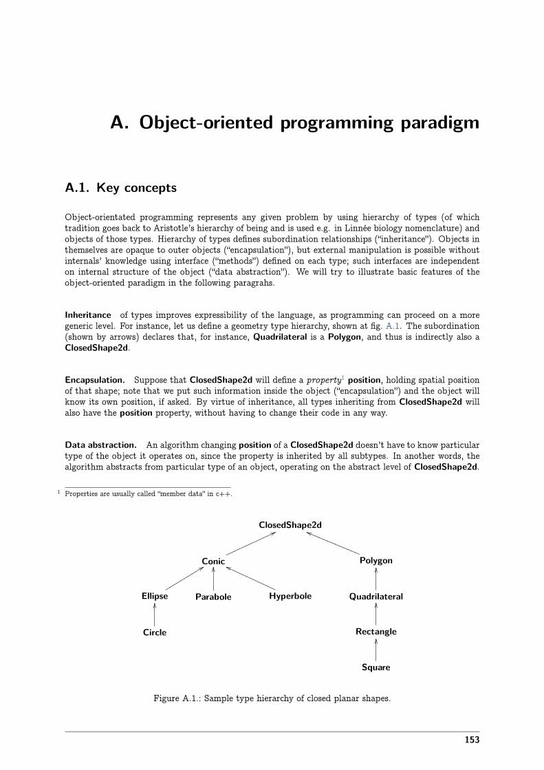
A. Object-oriented programming paradigm

A.1. Key concepts

Object-orientated programming represents any given problem by using hierarchy of types (of whichtradition goes back to Aristotle’s hierarchy of being and is used e.g. in Linnée biology nomenclature) andobjects of those types. Hierarchy of types defines subordination relationships (“inheritance”). Objects inthemselves are opaque to outer objects (“encapsulation”), but external manipulation is possible withoutinternals’ knowledge using interface (“methods”) defined on each type; such interfaces are independenton internal structure of the object (“data abstraction”). We will try to illustrate basic features of theobject-oriented paradigm in the following paragrahs.

Inheritance of types improves expressibility of the language, as programming can proceed on a moregeneric level. For instance, let us define a geometry type hierarchy, shown at fig. A.1. The subordination(shown by arrows) declares that, for instance, Quadrilateral is a Polygon, and thus is indirectly also aClosedShape2d.

Encapsulation. Suppose that ClosedShape2d will define a property1 position, holding spatial positionof that shape; note that we put such information inside the object (“encapsulation”) and the object willknow its own position, if asked. By virtue of inheritance, all types inheriting from ClosedShape2d willalso have the position property, without having to change their code in any way.

Data abstraction. An algorithm changing position of a ClosedShape2d doesn’t have to know particulartype of the object it operates on, since the property is inherited by all subtypes. In another words, thealgorithm abstracts from particular type of an object, operating on the abstract level of ClosedShape2d.

1 Properties are usually called “member data” in c++.

ClosedShape2d

Conic

66nnnnnnnnnnnnPolygon

hhRRRRRRRRRRRRR

Ellipse

99rrrrrrrrrrParabole

OO

Hyperbole

hhPPPPPPPPPPPPQuadrilateral

OO

Circle

OO

Rectangle

OO

Square

OO

Figure A.1.: Sample type hierarchy of closed planar shapes.

153

Polymorphism. If the user wanted to know a ClosedShape2d to return its area, we no longer can stay onthe abstract level, since area computation will be different for subtypes of ClosedShape2d. An algorithminterested in area would have to know about each subtype’s internals and, depending on the subtype,have different branches to compute area from those internals; this would, however, break encapsulationand the algorithm would have to be modified for each type added to the hierarchy.

Instead, only abstract interface will be declared in the ClosedShape2d class, a method2 area() computingarea; implementation of this interface will have to be done in each derived class, but the interface itselfwill be the same for all subtypes. Then, when area() method of an object is called, the object willinternally decide, based on its own type, which implementation to call, so that a Square calls Square’simplementation. Such decision based on subtype is called virtual dispatch and has to be done at runtime(so called “late binding”); the corresponding method is a virtual method. This allows a Square to appearas a ClosedShape2d on the interface level, but still function as Square (“polymorphism”).

area() dispatches based only on one subtype, of the instance itself. In some cases, it makes sense todispatch based on multiple types. For instance, computing overlap area between 2 ClosedShape2dswill require knowledge about both types; the overlap(other) method would be dispatched based oncombination of type of the object as well as of other. Such behavior is called multiple dispatch ormultimethod.

A.2. Language support and performance

Different programing languages implement the object-oriented pattern differently and we should pointout implementations in languages used in Yade, i. e. c++ and Python.

C++ is strongly-typed language: types of objects must be known at compile-time and function callsare resolved at compile-time (early binding, static binding) with the exception of virtual functions, whichare by definition resolved at runtime (late binding). This design decision allows generation of code thatsuffers no performance penalty compared to plain c code, with the exception of virtual functions.

Data encapsulation can be enforced by imposing access level on member data/methods:

private, where only object of this class access the data (or call the methods),

protected, where objects of this class and its derived (inheriting) subclasses can access the data),

public, where any object can access the data.

Virtual functions infer performance penaly (see Driesen and Hölzle [13] for detailed implementationanalysis and measurements), as instead of direct function call,3 the address of the function to call isdetermined by lookup in virtual function table4.

Multivirtual functions are not part of c++. The author of c++ published paper Pirkelbauer et al. [45],but their future addition to c++ is uncertain. To-day, they must be emulated with a hand-made dispatchmechanism, such as Smith [62] or Shopyrin [60], making use of simple virtual dispatch.

Python is dynamic language, said to be “duck-typed” – appropriate types are checked by existence ofproperties that are asked for; that provides high flexibility, allowing, for example, to pass an unrelatedobject where a file is required, as long as this object’s type has all properties that are used.

In Python, every attribute access and method call results in dictionary (string → object map) lookup,which proceeds from class of the object itself and climbs up the class hierarchy, until found. This

2 Called “member function” in c++.3 Member functions (members) are generated as regular functions with first hidden parameter carrying pointer to the object’s

instance.4 Implementation details of virtual dispatch are not mandated by the c++ standard, but the vtable approach is used by major c++

compilers (the GNU compiler in particular)

154

means that all methods in Python are virtual. There are no access levels, hence all data members are“public” (using the c++ terminology). The distinction between member data/function is made only forconvenience, since functions are also objects (defining the special call attribute).

Multimethods can be emulated quite easily in Python (e.g. van Rossum [64]); for our (Yade) purposes,multimethods are only interesting for the c++ part.

155

B. Quaternions

Quaternions[51] are hypercomplex numbers with 3 imaginary components, invented by William Hamilton[18]. They take the form w + xi + yj + zk, being points in R4 space with base (1, i, j, k); the relationbetween the bases is such that

i2 = j2 = k2 = ijk = −1. (B.1)This equation allows to establish all products of the base elements, e.g. ij = k and ji = −k. Notethat multiplication is non-cummutative. There are several operations defined on quaternions we shouldmention.

Quaternion product is analogous to complex number product, using distribubtion law, and additionallyuses rules for base products:

pq = (w1 + x1i+ x2 j+ y2k)(w2 + x2i+ y2 j+ z2k) =

= w1w2 − x1x2 − y1y2 − z1z2+

+ (w1x2 + x1w2 + y1z2 − z1y2)i+

+ (w1y2 − x1z2 + y1w2 + z1x2)j+

+ (w1z2 + x1y2 − y1x2 + z1w2)k

(B.2)

The product is obviously not commutative, due to non-commutativity of base products.

Quaternion conjugate q∗ of a q = w+ xi+ yj+ zk is defined

q∗ = w− xi− yj− zk. (B.3)

Note that (q∗)∗ = q (involution); conjugation of product reverses the order, so that

(pq)∗ = q∗p∗. (B.4)

Quaternion norm ||q|| is defined as √qq∗,

||q|| =√qq∗ =

√q∗q =

√w2 + x2 + y2 + z2, (B.5)

same as euclidean norm in the corresponding R4 space.

Quaternion inverse q−1 is such that qq−1 = 1. It can be shown that it is satisfied by

q−1 =q∗

||q||2, (B.6)

leading to identity of inverse and conjugate q−1 = q∗ for unit quaternions.

157

B.1. Unit quaternions as spatial rotations

Unit quaternions can represent spatial rotations [52]; in this section, unit length of all quaternions istacitly assumed.

In geometry, quaternions coefficients are usually written as scalar in R (the real part) plus vector in R3

(the imaginary part), so that

q = w+ xi+ yj+ zk = w+ u (B.7)

algebraic rules are then formally enriched by vector multiplication

mn = m× n−m · n (B.8)

defined in terms of regular scalar and vector product of vectors.

Vector rotation. It can be shown [52] that rotating R3 vector a around normalized axis u by angle ϑ,yielding transformed a ′, can be expressed by quaternion product

q = cos ϑ2+ u sin ϑ

2(B.9)

a ′ = qaq−1 (B.10)= qaq∗ (since ||q|| = 1) (B.11)

Conversion to axis-angle representation. Relationship inverse to (B.9) gives decomposition of quater-nion to its axis and angle components. Using the (B.7) notation, if |u| > 0, then

qϑ = 2 arccosw, qu = u. (B.12)

The case |u| = 0 implies cos ϑ/2 = 1, therefore ϑ = 2nπ. It follows that qϑ = 0 and qu is arbitrary unitvector.

Conversion to and from rotation vector. Quaternion q can be expressed as rotation vector a simplyas a = qϑqu. In the other sense, rotation vector a can be expressed as quaternion, using the (B.7) form,

q = cos |a|2

+ a sin |a|

2. (B.13)

Aligning 2 vectors. Given 2 vectors a, b, we want to find quaternion q = Align(a,b) such thatb = qaq∗. Computing auxiliary unit bisector c = ’a+ b, we can express (from scalar product geometricalinterpretation)

cos ϑ2=

a · c|a|

. (B.14)

The angle part, u sin ϑ/2 from (B.7), can be found as

a× c

|a|=

|a| sin ϑ2u

|a|= u sin ϑ

2. (B.15)

Finally, we come to the solution

q =a · c|a|

+a× c

|a|=

a · ’a+ b

|a|+

a× ’a+ b

|a|= Align(a,b). (B.16)

The operation is obviously meaningful only if |a| = 0.

158

Rotation composition Applying two consecutive rotations q and p on the vector shows that it isequivalent to applying composed rotation in the form of quaternion product pq (note the reverse order):

q(pap∗)q∗ = qpap∗q∗ = (qp)a(qp)∗ (B.17)

As a special case, this shows that conjugate quaternion q∗ is rotation in the opposite sense, sinceq∗(qaq∗)q∗∗ = a. Rotations can be composed arbitrarily, in general

qn(· · · (q2(q1aq∗1)q

∗2) · · · )q∗

n = (qn · · ·q2q1)a(qn · · ·q2q1)∗ (B.18)

Rotation interpolation Quaternions allow for easy and efficient interpolation between two quaternionsp and q, parametrized on t ∈ {0 . . . 1} [61]. Since rotations are points on unit 4-dimensional hyper-sphere (quaternions representing rotations satisfy ||q|| = 1), this interpolation is called spherical linearinterpolation (“slerp”). It follows from series expansion and quaternion unit length that

qt = cos tϑ2+ v sin tϑ

2(B.19)

The interpolation over t ∈ ⟨0 . . . 1⟩

Slerp(p, q; t) = p(p∗q)t (B.20)

is shortest path (geodesic on the hypersphere) between p and q with constant 3d angular velocity vectorin the sense of the v unit vector representing rotation axis. This interpolation is frequently used incomputer graphics.

B.2. Comparison of spatial rotation representations

There are 4 widespread ways to represent rotations:

Rotation matrix (direction cosine matrix, DCM), 3×3 matrix of which 3 columns are transformed basevectors x ′, y ′, z ′. Rotation composition is done by matrix multiplication in the reverse order.Since spatial rotations space is 3-dimensional, matrix elements are not independent; transformedbase vectors must be orthonormal.

In numerical simulations, rotation matrices must be (frequently) renormalized, as accumulatingnumerical errors leads to loss of orthonormality, introducing distorsion. The cost of re-normalizationis evaluation of 3 square roots (when using the Gram-Schmidt algorithm), compared to signle squareroot evaluation involved in quaternion normalization.

Euler angles, 3 angles of independent rotations around axes appiled consecutively [15]. There are differ-ent conventions which rotation axes are used and in what order; it can be any non-homogeneoustriple of x, y, z, which are originally coincident with frame of reference axis. Two of 24 possibleconventions are widely used, z-x-z and z-y-x (known as yaw-roll-pitch).

The convention called z-x-z rotates around z (coincident with z of the frame of reference), thenaround now-rotated x and finally around rotated z. This convention is usually meant when “Eulerangles” is used without further specification.

The “yaw-pitch-roll” convention is used in aeronautics rotates the frame of reference consecutivelyaround z, y (once rotated) and x (twice rotated) axes and has intuitive meaning for spacecraftorientation, whence the “yaw-roll-pitch” name.

Rotation composition can be done by matrix multiplication of corresponding rotation matrices,which are themselves product of 3 matrices representing each rotation separately and multiplied inproper order.

The chief disadvantage of using any of the Euler angles is their singularity at poles, known asgimbal lock; for instance, the pitch of π/2 leads to infinite possible combinations of yaw and rollangles to arrive at given configuration (e.g. roll angle can be zero, while only yaw angle changes).

159

Angle/axis (angle to turn around normalized axis) with clear geometrical meaning. The disadvatage isthat rotation composition is possible only indirectly, by performing conversion to another repre-sentation first. Multiplying axis by angle, rotation vector is obtained.

Quaternions were introduced above; among their advantages is easy rotation composition and lack ofsingularities (in contrast to Euler angles). Like rotation matrices, quaternions must be renormal-ized to avoid accumulation of numerical errros; however, quaternion normalization involves onlyevaluation of one square root.

One disadvatage is that rotating vector by quaternion performs 39 multiples and adds, whereasrotating by rotation matrix needs only 15 such operations. For that reason, some libraries createrotation matrix from the quaternion internally and multiply by that matrix instead; the (orthonor-mal) matrix R can be directly computed from q = w+ xi+ yj+ zk

R =

Ñw2 + x2 − y2 − z2 2xy− 2wz 2xz+ 2wy

2xy+ 2wz w2 − x2 + y2 − z2 2yz− 2wx

2xz− 2wy 2yz+ 2wx w2 − x2 − y2 + z2

é. (B.21)

160

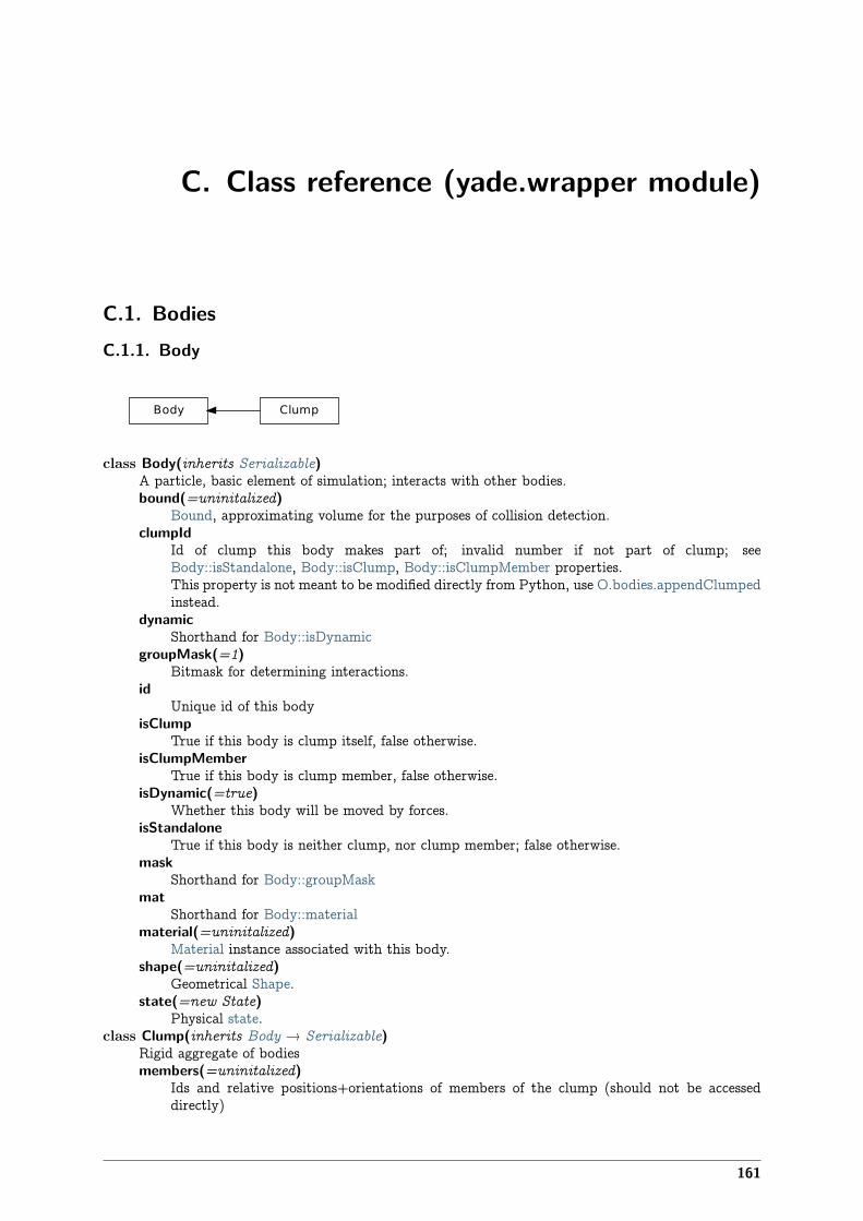
C. Class reference (yade.wrapper module)

C.1. BodiesC.1.1. Body

Body Clump

class Body(inherits Serializable)A particle, basic element of simulation; interacts with other bodies.bound(=uninitalized)

Bound, approximating volume for the purposes of collision detection.clumpId

Id of clump this body makes part of; invalid number if not part of clump; seeBody::isStandalone, Body::isClump, Body::isClumpMember properties.This property is not meant to be modified directly from Python, use O.bodies.appendClumpedinstead.

dynamicShorthand for Body::isDynamic

groupMask(=1)Bitmask for determining interactions.

idUnique id of this body

isClumpTrue if this body is clump itself, false otherwise.

isClumpMemberTrue if this body is clump member, false otherwise.

isDynamic(=true)Whether this body will be moved by forces.

isStandaloneTrue if this body is neither clump, nor clump member; false otherwise.

maskShorthand for Body::groupMask

matShorthand for Body::material

material(=uninitalized)Material instance associated with this body.

shape(=uninitalized)Geometrical Shape.

state(=new State)Physical state.

class Clump(inherits Body → Serializable)Rigid aggregate of bodiesmembers(=uninitalized)

Ids and relative positions+orientations of members of the clump (should not be accesseddirectly)

161

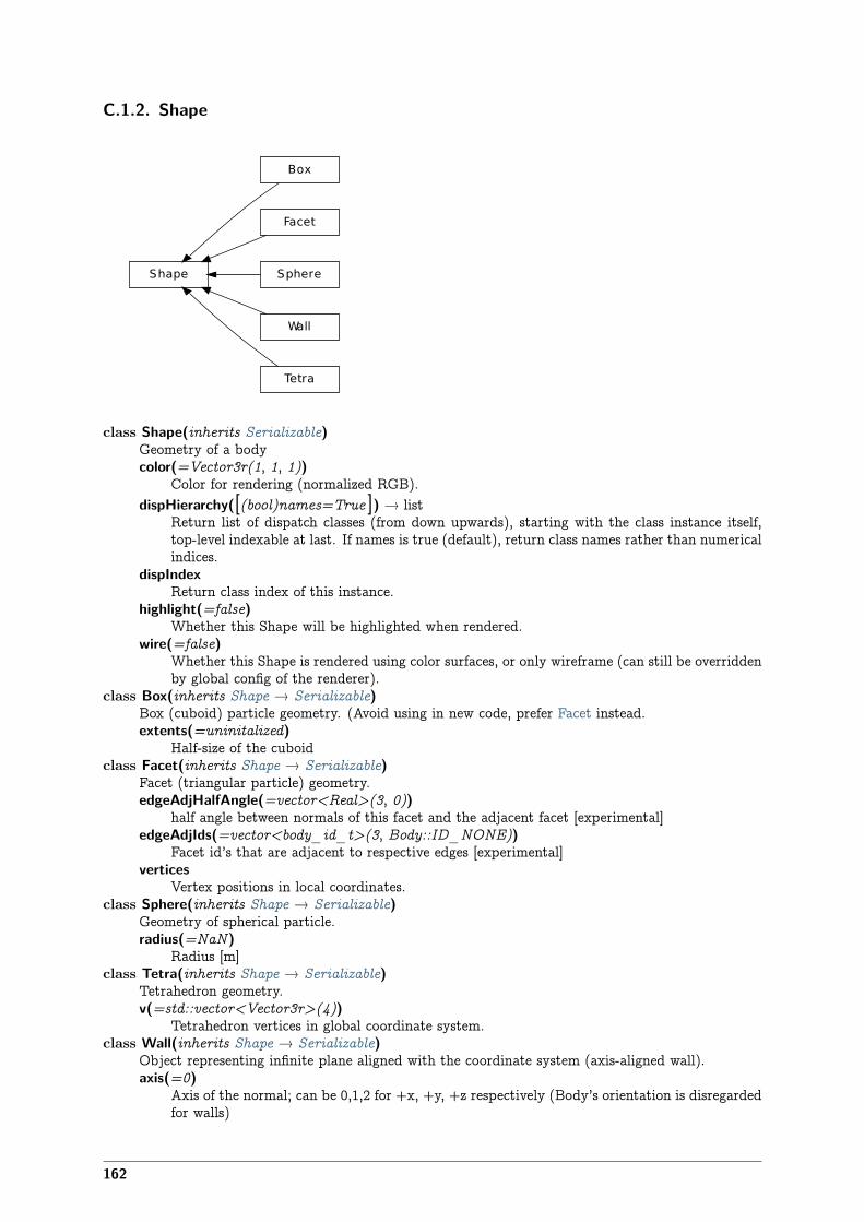
C.1.2. Shape

Shape

Box

Facet

Sphere

Wall

Tetra

class Shape(inherits Serializable)Geometry of a bodycolor(=Vector3r(1, 1, 1))

Color for rendering (normalized RGB).dispHierarchy([(bool)names=True ]) → list

Return list of dispatch classes (from down upwards), starting with the class instance itself,top-level indexable at last. If names is true (default), return class names rather than numericalindices.

dispIndexReturn class index of this instance.

highlight(=false)Whether this Shape will be highlighted when rendered.

wire(=false)Whether this Shape is rendered using color surfaces, or only wireframe (can still be overriddenby global config of the renderer).

class Box(inherits Shape → Serializable)Box (cuboid) particle geometry. (Avoid using in new code, prefer Facet instead.extents(=uninitalized)

Half-size of the cuboidclass Facet(inherits Shape → Serializable)

Facet (triangular particle) geometry.edgeAdjHalfAngle(=vector<Real>(3, 0))

half angle between normals of this facet and the adjacent facet [experimental]edgeAdjIds(=vector<body_id_t>(3, Body::ID_NONE))

Facet id’s that are adjacent to respective edges [experimental]vertices

Vertex positions in local coordinates.class Sphere(inherits Shape → Serializable)

Geometry of spherical particle.radius(=NaN)

Radius [m]class Tetra(inherits Shape → Serializable)

Tetrahedron geometry.v(=std::vector<Vector3r>(4))

Tetrahedron vertices in global coordinate system.class Wall(inherits Shape → Serializable)

Object representing infinite plane aligned with the coordinate system (axis-aligned wall).axis(=0)

Axis of the normal; can be 0,1,2 for +x, +y, +z respectively (Body’s orientation is disregardedfor walls)

162

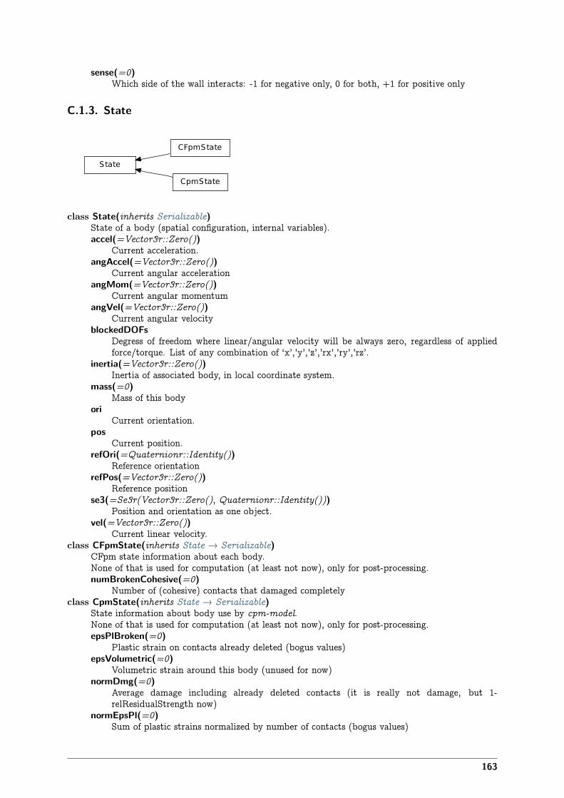
sense(=0)Which side of the wall interacts: -1 for negative only, 0 for both, +1 for positive only

C.1.3. State

State

CFpmState

CpmState

class State(inherits Serializable)State of a body (spatial configuration, internal variables).accel(=Vector3r::Zero())

Current acceleration.angAccel(=Vector3r::Zero())

Current angular accelerationangMom(=Vector3r::Zero())

Current angular momentumangVel(=Vector3r::Zero())

Current angular velocityblockedDOFs

Degress of freedom where linear/angular velocity will be always zero, regardless of appliedforce/torque. List of any combination of ‘x’,’y’,’z’,’rx’,’ry’,’rz’.

inertia(=Vector3r::Zero())Inertia of associated body, in local coordinate system.

mass(=0)Mass of this body

oriCurrent orientation.

posCurrent position.

refOri(=Quaternionr::Identity())Reference orientation

refPos(=Vector3r::Zero())Reference position

se3(=Se3r(Vector3r::Zero(), Quaternionr::Identity()))Position and orientation as one object.

vel(=Vector3r::Zero())Current linear velocity.

class CFpmState(inherits State → Serializable)CFpm state information about each body.None of that is used for computation (at least not now), only for post-processing.numBrokenCohesive(=0)

Number of (cohesive) contacts that damaged completelyclass CpmState(inherits State → Serializable)

State information about body use by cpm-model.None of that is used for computation (at least not now), only for post-processing.epsPlBroken(=0)

Plastic strain on contacts already deleted (bogus values)epsVolumetric(=0)

Volumetric strain around this body (unused for now)normDmg(=0)

Average damage including already deleted contacts (it is really not damage, but 1-relResidualStrength now)

normEpsPl(=0)Sum of plastic strains normalized by number of contacts (bogus values)

163

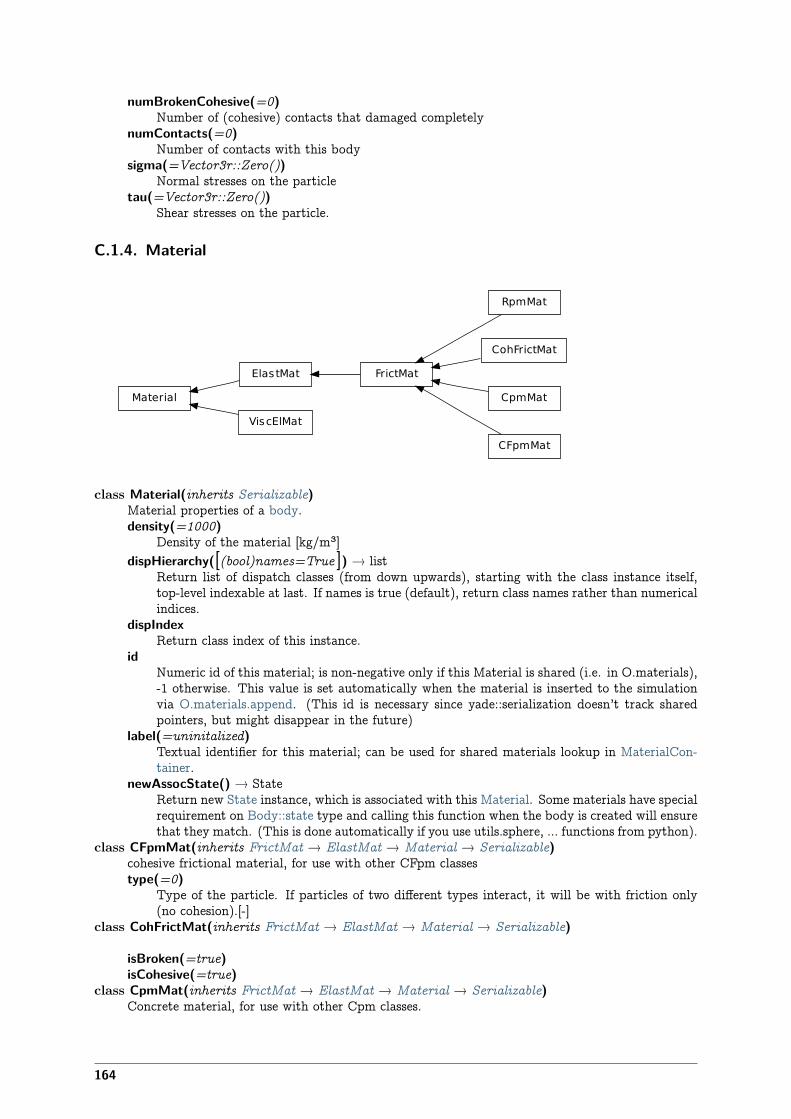
numBrokenCohesive(=0)Number of (cohesive) contacts that damaged completely

numContacts(=0)Number of contacts with this body

sigma(=Vector3r::Zero())Normal stresses on the particle

tau(=Vector3r::Zero())Shear stresses on the particle.

C.1.4. Material

Material

RpmMat

FrictMatElastMat

CohFrictMat

CpmMat

CFpmMat

ViscElMat

class Material(inherits Serializable)Material properties of a body.density(=1000)

Density of the material [kg/m³]dispHierarchy([(bool)names=True ]) → list

Return list of dispatch classes (from down upwards), starting with the class instance itself,top-level indexable at last. If names is true (default), return class names rather than numericalindices.

dispIndexReturn class index of this instance.

idNumeric id of this material; is non-negative only if this Material is shared (i.e. in O.materials),-1 otherwise. This value is set automatically when the material is inserted to the simulationvia O.materials.append. (This id is necessary since yade::serialization doesn’t track sharedpointers, but might disappear in the future)

label(=uninitalized)Textual identifier for this material; can be used for shared materials lookup in MaterialCon-tainer.

newAssocState() → StateReturn new State instance, which is associated with this Material. Some materials have specialrequirement on Body::state type and calling this function when the body is created will ensurethat they match. (This is done automatically if you use utils.sphere, … functions from python).

class CFpmMat(inherits FrictMat → ElastMat → Material → Serializable)cohesive frictional material, for use with other CFpm classestype(=0)

Type of the particle. If particles of two different types interact, it will be with friction only(no cohesion).[-]

class CohFrictMat(inherits FrictMat → ElastMat → Material → Serializable)

isBroken(=true)isCohesive(=true)

class CpmMat(inherits FrictMat → ElastMat → Material → Serializable)Concrete material, for use with other Cpm classes.

164

Note: Density is initialized to 4800 kgm�³automatically, which gives approximate 2800 kgm�³on 0.5 density packing.The model is contained in externally defined macro CPM_MATERIAL_MODEL, which featuresdamage in tension, plasticity in shear and compression and rate-dependence. For commercial rea-sons, rate-dependence and compression-plasticity is not present in reduced version of the model,used when CPM_MATERIAL_MODEL is not defined. The full model will be described in de-tail in my (Václav Šmilauer) thesis along with calibration procedures (rigidity, poisson’s ratio,compressive/tensile strength ratio, fracture energy, behavior under confinement, rate-dependentbehavior).Even the public model is useful enough to run simulation on concrete samples, such as uniaxialtension-compression test.G_over_E(=NaN)

Ratio of normal/shear stiffness at interaction level [-]dmgRateExp(=0)

Exponent for normal viscosity function. [-]dmgTau(=-1, deactivated if negative)

Characteristic time for normal viscosity. [s]epsCrackOnset(=NaN)

Limit elastic strain [-]isoPrestress(=0)

Isotropic prestress of the whole specimen. [Pa]neverDamage(=false)

If true, no damage will occur (for testing only).plRateExp(=0)

Exponent for visco-plasticity function. [-]plTau(=-1, deactivated if negative)

Characteristic time for visco-plasticity. [s]relDuctility(=NaN)

Relative ductility, for damage evolution law peak right-tangent. [-]sigmaT(=NaN)

Initial cohesion [Pa]class ElastMat(inherits Material → Serializable)

Purely elastic material.poisson(=.25)

Poisson’s ratio [-]young(=1e9)

Young’s modulus [Pa]class FrictMat(inherits ElastMat → Material → Serializable)

Material with internal friction.frictionAngle(=.5)

Internal friction angle (in radians) [-]class RpmMat(inherits FrictMat → ElastMat → Material → Serializable)

Rock material, for use with other Rpm classes.Brittleness(=0)

One of destruction parameters. [-] //(Needs to be reworked)G_over_E(=1)

Ratio of normal/shear stiffness at interaction level. [-]exampleNumber(=0)

Number of the specimen. This value is equal for all particles of one specimen. [-]initCohesive(=false)

The flag shows, whether particles of this material can be cohesive. [-]stressCompressMax(=0)

Maximal strength for compression. The main destruction parameter. [Pa] //(Needs to bereworked)

class ViscElMat(inherits Material → Serializable)Material for simple viscoelastic model of contact.Note: Shop::getViscoelasticFromSpheresInteraction (andutils.getViscoelasticFromSpheresInteraction in python) compute kn, cn, ks, cs from analyti-

165

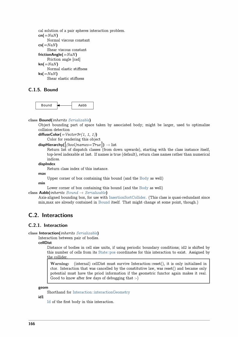
cal solution of a pair spheres interaction problem.cn(=NaN)

Normal viscous constantcs(=NaN)

Shear viscous constantfrictionAngle(=NaN)

Friction angle [rad]kn(=NaN)

Normal elastic stiffnessks(=NaN)

Shear elastic stiffness

C.1.5. Bound

Bound Aabb

class Bound(inherits Serializable)Object bounding part of space taken by associated body; might be larger, used to optimalizecollision detectiondiffuseColor(=Vector3r(1, 1, 1))

Color for rendering this objectdispHierarchy([(bool)names=True ]) → list

Return list of dispatch classes (from down upwards), starting with the class instance itself,top-level indexable at last. If names is true (default), return class names rather than numericalindices.

dispIndexReturn class index of this instance.

maxUpper corner of box containing this bound (and the Body as well)

minLower corner of box containing this bound (and the Body as well)

class Aabb(inherits Bound → Serializable)Axis-aligned bounding box, for use with InsertionSortCollider. (This class is quasi-redundant sincemin,max are already contained in Bound itself. That might change at some point, though.)

C.2. InteractionsC.2.1. Interactionclass Interaction(inherits Serializable)

Interaction between pair of bodies.cellDist

Distance of bodies in cell size units, if using periodic boundary conditions; id2 is shifted bythis number of cells from its State::pos coordinates for this interaction to exist. Assigned bythe collider.

Warning: (internal) cellDist must survive Interaction::reset(), it is only initialized inctor. Interaction that was cancelled by the constitutive law, was reset() and became onlypotential must have the priod information if the geometric functor again makes it real.Good to know after few days of debugging that :-)

geomShorthand for Interaction::interactionGeometry

id1Id of the first body in this interaction.

166

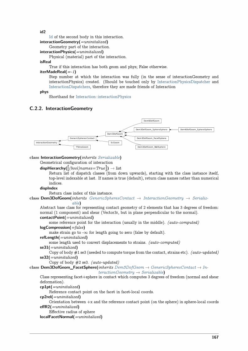
id2Id of the second body in this interaction.

interactionGeometry(=uninitalized)Geometry part of the interaction.

interactionPhysics(=uninitalized)Physical (material) part of the interaction.

isRealTrue if this interaction has both geom and phys; False otherwise.

iterMadeReal(=-1)Step number at which the interaction was fully (in the sense of interactionGeometry andinteractionPhysics) created. (Should be touched only by InteractionPhysicsDispatcher andInteractionDispatchers, therefore they are made friends of Interaction

physShorthand for Interaction::interactionPhysics

C.2.2. InteractionGeometry

InteractionGeometry

Dem6DofGeom

Dem3DofGeom

GenericSpheresContact

Dem3DofGeom_SphereSphere

Dem3DofGeom_FacetSphere

TTetraGeom Dem3DofGeom_WallSphere

ScGeom

Dem6DofGeom_SphereSphere

class InteractionGeometry(inherits Serializable)Geometrical configuration of interactiondispHierarchy([(bool)names=True ]) → list

Return list of dispatch classes (from down upwards), starting with the class instance itself,top-level indexable at last. If names is true (default), return class names rather than numericalindices.

dispIndexReturn class index of this instance.

class Dem3DofGeom(inherits GenericSpheresContact → InteractionGeometry → Serializ-able)

Abstract base class for representing contact geometry of 2 elements that has 3 degrees of freedom:normal (1 component) and shear (Vector3r, but in plane perpendicular to the normal).contactPoint(=uninitalized)

some reference point for the interaction (usually in the middle). (auto-computed)logCompression(=false)

make strain go to -∞ for length going to zero (false by default).refLength(=uninitalized)

some length used to convert displacements to strains. (auto-computed)se31(=uninitalized)

Copy of body #1 se3 (needed to compute torque from the contact, strains etc). (auto-updated)se32(=uninitalized)

Copy of body #2 se3. (auto-updated)class Dem3DofGeom_FacetSphere(inherits Dem3DofGeom→ GenericSpheresContact→ In-

teractionGeometry → Serializable)Class representing facet+sphere in contact which computes 3 degrees of freedom (normal and sheardeformation).cp1pt(=uninitalized)

Reference contact point on the facet in facet-local coords.cp2rel(=uninitalized)

Orientation between +x and the reference contact point (on the sphere) in sphere-local coordseffR2(=uninitalized)

Effective radius of spherelocalFacetNormal(=uninitalized)

167

Unit normal of the facet plane in facet-local coordinatesclass Dem3DofGeom_SphereSphere(inherits Dem3DofGeom → GenericSpheresContact →

InteractionGeometry → Serializable)Class representing 2 spheres in contact which computes 3 degrees of freedom (normal and sheardeformation).cp1rel(=uninitalized)

Sphere’s #1 relative orientation of the contact point with regards to sphere-local +x axis(quasi-constant)

cp2rel(=uninitalized)Same as cp1rel, but for sphere #2.

effR1(=uninitalized)Effective radius of sphere #1; can be smaller/larger than refR1 (the actual radius), but quasi-constant throughout interaction life

effR2(=uninitalized)Same as effR1, but for sphere #2.

class Dem3DofGeom_WallSphere(inherits Dem3DofGeom → GenericSpheresContact → In-teractionGeometry → Serializable)

Representation of contact between wall and sphere, based on Dem3DofGeom.cp1pt(=uninitalized)

initial contact point on the wall, relative to the current contact pointcp2rel(=uninitalized)

orientation between +x and the reference contact point (on the sphere) in sphere-local coordseffR2(=uninitalized)

effective radius of sphereclass Dem6DofGeom(inherits Dem3DofGeom → GenericSpheresContact → InteractionGe-

ometry → Serializable)Abstract class for providing torsion and bending, in addition to inherited normal and shear strains.

class Dem6DofGeom_SphereSphere(inherits Dem3DofGeom_SphereSphere →Dem3DofGeom → GenericSpheresContact → In-teractionGeometry → Serializable)

Class representing 2 sphere in contact which computes 6 degrees of freedom (normal, shear, bendingand twisting deformation)initRelOri12(=uninitalized)

Initial relative orientation of spheres, used for bending and twisting computation.class GenericSpheresContact(inherits InteractionGeometry → Serializable)

Class uniting ScGeom and Dem3DofGeom, for the purposes of GlobalStiffnessTimeStepper. (Itmight be removed inthe future). Do not use this class directly.normal(=uninitalized)

Unit vector oriented along the interaction. (auto-updated)refR1(=uninitalized)

Reference radius of particle #1. (auto-computed)refR2(=uninitalized)

Reference radius of particle #2. (auto-computed)class ScGeom(inherits GenericSpheresContact → InteractionGeometry → Serializable)

Class representing geometry of two spheres in contact. The contact has 3 DOFs (normal and2×shear) and uses incremental algorithm for updating shear. (For shear formulated in total dis-placements and rotations, see Dem3DofGeom and related classes).We use symbols x, v, ω respectively for position, linear and angular velocities (all in global coor-dinates) and r for particles radii; subscripted with 1 or 2 to distinguish 2 spheres in contact. Thenwe compute unit contact normal

n =x2 − x1

||x2 − x1||

Relative velocity of spheres is then

v12 = (v2 +ω2 × (−r2n)) − (v1 +ω1 × (r1n))

and its shear component

∆vs12 = v12 − (n · v12)n.

168

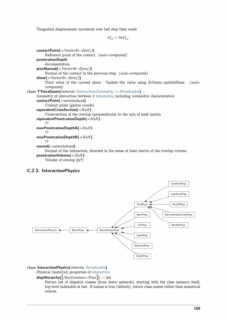
Tangential displacement increment over last step then reads

xs12 = ∆tvs12.

contactPoint(=Vector3r::Zero())Reference point of the contact. (auto-computed)

penetrationDepthdocumentation

prevNormal(=Vector3r::Zero())Normal of the contact in the previous step. (auto-computed)

shear(=Vector3r::Zero())Total value of the current shear. Update the value using ScGeom::updateShear. (auto-computed)

class TTetraGeom(inherits InteractionGeometry → Serializable)Geometry of interaction between 2 tetrahedra, including volumetric characteristicscontactPoint(=uninitalized)

Contact point (global coords)equivalentCrossSection(=NaN)

Cross-section of the overlap (perpendicular to the axis of least inertiaequivalentPenetrationDepth(=NaN)

??maxPenetrationDepthA(=NaN)

??maxPenetrationDepthB(=NaN)

??normal(=uninitalized)

Normal of the interaction, directed in the sense of least inertia of the overlap volumepenetrationVolume(=NaN)

Volume of overlap [m³]

C.2.3. InteractionPhysics

InteractionPhys ics

FrictPhys

NormShearPhysNormPhys

CohFrictPhys

RpmPhys

CapillaryPhys

CSPhys

ViscElPhys

CpmPhys

MomentPhys

NormalInelasticityPhys

CFpmPhys

MindlinPhys

class InteractionPhysics(inherits Serializable)Physical (material) properties of interaction.dispHierarchy([(bool)names=True ]) → list

Return list of dispatch classes (from down upwards), starting with the class instance itself,top-level indexable at last. If names is true (default), return class names rather than numericalindices.

169

dispIndexReturn class index of this instance.

class CFpmPhys(inherits NormShearPhys→ NormPhys→ InteractionPhysics→ Serializable)Representation of a single interaction of the CFpm type, storage for relevant parametersFnMax(=0)

Defines the maximum admissible normal force in traction Fn-Max=tensileStrength*crossSection, with crossSection=pi*Rmin^2. [Pa]

FsMax(=0)Defines the maximum admissible tangential force in shear FsMax=cohesion*FnMax, withcrossSection=pi*Rmin^2. [Pa]

cumulativeRotation(=0)Cumulated rotation... [-]

frictionAngle(=0)defines Coulomb friction. [deg]

initD(=0)equilibrium distance for particles. Computed as the initial interparticular distance whenbonded particle interact. initD=0 for non cohesive interactions.

initialOrientation1(=Quaternionr(1.0, 0.0, 0.0, 0.0))Used for moment computation.

initialOrientation2(=Quaternionr(1.0, 0.0, 0.0, 0.0))Used for moment computation.

isCohesive(=false)If false, particles interact in a frictional way. If true, particles are bonded regarding the givencohesion and tensileStrength.

kr(=0)Defines the stiffness to compute the resistive moment in rotation. [-]

maxBend(=0)Defines the maximum admissible resistive moment in rotation Mtmax=maxBend*Fn,maxBend=eta*meanRadius. [m]

moment_bending(=Vector3r::Zero())[N.m]

moment_twist(=Vector3r::Zero())[N.m]

prevNormal(=Vector3r::Zero())Normal to the contact at previous time step.

strengthSoftening(=0)Defines the softening when Dtensile is reached to avoid explosion. Typically, when D >Dtensile, Fn=FnMax - (kn/strengthSoftening)*(Dtensile-D). [-]

tanFrictionAngle(=0)Tangent of frictionAngle. [-]

class CSPhys(inherits NormShearPhys → NormPhys → InteractionPhysics → Serializable)Physical properties for Cundall&Strack constitutive law, created by Ip2_2xFrictMat_CSPhys.frictionAngle(=NaN)

Friction angle of the interaction. (auto-computed)tanFrictionAngle(=NaN)

Precomputed tangent of CSPhys::frictionAngle. (auto-computed)class CapillaryPhys(inherits FrictPhys→ NormShearPhys→ NormPhys→ InteractionPhysics→ Serializable)

Physics (of interaction) for Law2_ScGeom_CapillaryPhys_Capillarity. Rk: deprecated -> needssome work to be conform with the new formalism!CapillaryPressure(=0.)

Value of the capillary pressure Uc defines as Ugas-UliquidDelta1(=0.)

Defines the surface area wetted by the meniscus on the smallest grains of radius R1 (R1<R2)Delta2(=0.)

Defines the surface area wetted by the meniscus on the biggest grains of radius R2 (R1<R2)Fcap(=Vector3r::Zero())

Capillary Force produces by the presence of the meniscus

170

Vmeniscus(=0.)Volume of the menicus

fusionNumber(=0.)Indicates the number of meniscii that overlap with this one

meniscus(=false)Presence of a meniscus if true

class CohFrictPhys(inherits FrictPhys→ NormShearPhys→ NormPhys→ InteractionPhysics→ Serializable)cohesionBroken(=true)

is cohesion active? will be set false when a fragile contact is brokencohesionDisablesFriction(=false)

is shear strength the sum of friction and adhesion or only adhesion?currentContactOrientation(=Quaternionr(1.0, 0.0, 0.0, 0.0))fragile(=true)

do cohesion disapear when contact strength is exceeded?initialContactOrientation(=Quaternionr(1.0, 0.0, 0.0, 0.0))initialOrientation1(=Quaternionr(1.0, 0.0, 0.0, 0.0))initialOrientation2(=Quaternionr(1.0, 0.0, 0.0, 0.0))initialPosition1(=Vector3r(0, 0, 0))initialPosition2(=Vector3r(0, 0, 0))kr(=0)

rotational stiffness [N.m/rad]moment_bending(=Vector3r(0, 0, 0))moment_twist(=Vector3r(0, 0, 0))normalAdhesion(=0)

tensile strengthorientationToContact1(=Quaternionr(1.0, 0.0, 0.0, 0.0))orientationToContact2(=Quaternionr(1.0, 0.0, 0.0, 0.0))shearAdhesion(=0)

cohesive part of the shear strength (a frictional term might be added depending on Law2_-ScGeom_CohFrictPhys_ElasticPlastic::cohesionDisablesFriction)

twistCreep(=Quaternionr(1.0, 0.0, 0.0, 0.0))class CpmPhys(inherits NormShearPhys → NormPhys → InteractionPhysics → Serializable)

Representation of a single interaction of the Cpm type: storage for relevant parameters.Evolution of the contact is governed by Law2_Dem3DofGeom_CpmPhys_Cpm, that includesdamage effects and chages of parameters inside CpmPhys. See cpm-model for details.E(=NaN)

normal modulus (stiffness / crossSection) [Pa]Fn

Magnitude of normal force.Fs

Magnitude of shear forceG(=NaN)

shear modulus [Pa]crossSection(=NaN)

equivalent cross-section associated with this contact [m²]dmgOverstress(=0)

damage viscous overstress (at previous step or at current step)dmgRateExp(=0)

exponent in the rate-dependent damage evolutiondmgStrain(=0)

damage strain (at previous or current step)dmgTau(=-1)

characteristic time for damage (if non-positive, the law without rate-dependence is used)epsCrackOnset(=NaN)

strain at which the material starts to behave non-linearlyepsFracture(=NaN)

strain where the damage-evolution law tangent from the top (epsCrackOnset) touches the axis;

171

since the softening law is exponential, this doesn’t mean that the contact is fully damaged atthis point, that happens only asymptotically

epsNCurrent normal strain

epsNPl(=0)normal plastic strain (initially zero)

epsPlSum(=0)cummulative shear plastic strain measure (scalar) on this contact

epsTTransversal strain (not used)

epsTrans(=0)Transversal strain (perpendicular to the contact axis)

isCohesive(=false)if not cohesive, interaction is deleted when distance is greater than zero.

isoPrestress(=0)“prestress” of this link (used to simulate isotropic stress)

kappaD(=0)Up to now maximum normal strain (semi-norm), non-decreasing in time.

neverDamage(=false)the damage evolution function will always return virgin state

omegaDamage internal variable

plRateExp(=0)exponent in the rate-dependent viscoplasticity

plTau(=-1)characteristic time for viscoplasticity (if non-positive, no rate-dependence for shear)

relResidualStrengthRelative residual strength

sigmaNCurrent normal stress

sigmaTCurrent shear stress

tanFrictionAngle(=NaN)tangens of internal friction angle [-]

undamagedCohesion(=NaN)virgin material cohesion [Pa]

class FrictPhys(inherits NormShearPhys → NormPhys → InteractionPhysics → Serializable)Interaction with frictionprevNormal(=Vector3r::Zero())

unit normal of the contact plane in previous steptangensOfFrictionAngle(=NaN)

tan of angle of frictionclass MindlinPhys(inherits FrictPhys → NormShearPhys → NormPhys → InteractionPhysics→ Serializable)

Representation of an interaction of the Mindlin type.kno(=0.0)

Constant value in the formulation of the normal stiffnesskso(=0.0)

Constant value in the formulation of the tangential stiffnessclass MomentPhys(inherits NormShearPhys → NormPhys → InteractionPhysics → Serializ-

able)Physical interaction properties for use with Law2_SCG_MomentPhys_CohesionlessMomentRota-tion, created by Ip2_MomentMat_MomentMat_MomentPhys.Eta(=0)

??cumulativeRotation(=0)

??frictionAngle(=0)

172

Friction angle [rad]initialOrientation1(=Quaternionr::Identity())

??initialOrientation2(=Quaternionr::Identity())

??kr(=0)

rolling stiffnessmoment_bending(=Vector3r::Zero())

??moment_twist(=Vector3r::Zero())

??prevNormal(=Vector3r::Zero())

Normal in the previous step.shear(=Vector3r::Zero())

??tanFrictionAngle(=0)

Tangent of friction angleclass NormPhys(inherits InteractionPhysics → Serializable)

Abstract class for interactions that have normal stiffness.kn(=NaN)

Normal stiffnessnormalForce(=Vector3r::Zero())

Normal force after previous step (in global coordinates).class NormShearPhys(inherits NormPhys → InteractionPhysics → Serializable)

Abstract class for interactions that have shear stiffnesses, in addition to normal stiffness. This classis used in the PFC3d-style stiffness timestepper.ks(=NaN)

Shear stiffnessshearForce(=Vector3r::Zero())

Shear force after previous step (in global coordinates).class NormalInelasticityPhys(inherits FrictPhys → NormShearPhys → NormPhys → Interac-

tionPhysics → Serializable)Physics (of interaction) for using Law2_ScGeom_NormalInelasticityPhys_NormalInelasticitycurrentContactOrientation(=Quaternionr::Identity())forMaxMoment(=1.0)

parameter stored for each interaction, and allowing to compute the maximum value of theexchanged torque : TorqueMax= forMaxMoment * NormalForce

initialContactOrientation(=Quaternionr::Identity())initialOrientation1(=Quaternionr::Identity())initialOrientation2(=Quaternionr::Identity())initialPosition1(=Vector3r::Zero())initialPosition2(=Vector3r::Zero())kr(=0.0)

the rolling stiffness of the rigidityorientationToContact1(=Quaternionr::Identity())orientationToContact2(=Quaternionr::Identity())previousFn(=0.0)

the value of the normal force at the last time steppreviousun(=0.0)

the value of this un at the last time stepunMax(=0.0)

the maximum value of penetration depth of the history of this interactionclass RpmPhys(inherits NormShearPhys → NormPhys → InteractionPhysics → Serializable)

Representation of a single interaction of the Cpm type: storage for relevant parameters.Evolution of the contact is governed by Law2_Dem3DofGeom_CpmPhys_Cpm, that includesdamage effects and chages of parameters inside CpmPhysE(=NaN)

normal modulus (stiffness / crossSection) [Pa]

173

G(=NaN)shear modulus [Pa]

crossSection(=0)equivalent cross-section associated with this contact [m²]

isCohesive(=false)if not cohesive, interaction is deleted when distance is greater than lengthMaxTension or lessthan lengthMaxCompression.

lengthMaxCompression(=0)Maximal penetration of particles during compression. If it is more, the interaction is deleted[m]

lengthMaxTension(=0)Maximal distance between particles during tension. If it is more, the interaction is deleted [m]

tanFrictionAngle(=NaN)tangens of internal friction angle [-]

class ViscElPhys(inherits FrictPhys → NormShearPhys → NormPhys → InteractionPhysics→ Serializable)InteractionPhysics created from ViscElMat, for use with Law2_ScGeom_ViscElPhys_Basic.cn(=NaN)

Normal viscous constantcs(=NaN)

Shear viscous constant

174

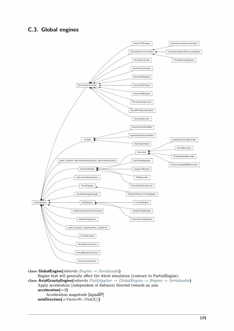
C.3. Global engines

GlobalEngine

KinemCTDEngine

BoundaryController

Collider

InsertionSortCollider

Law2_ScGeom_NormalInelasticityPhys_NormalInelasticity

SpatialQuickSortCollider

PeriodicEngine

TriaxialCompress ionEngine

TriaxialStressController

Peri3dController

CapillaryStressRecorder

Recorder

InteractionDispatchers

FlatGridCollider

ForceRecorder

GlobalStiffnessTimeStepper

TimeStepper

FacetTopologyAnalyzer

CpmStateUpdater

FieldApplier

Cohes iveFrictionalContactLaw

NewtonIntegrator

GravityEngine

TriaxialStateRecorder

PeriTriaxController

Law2_ScGeom_CapillaryPhys_Capillarity

ForceResetter

Cohes iveStateRPMRecorder

TetraVolumetricLaw

KinemCNLEngine

KinemCNSEngine

KinemCNDEngine

PeriIsoCompressor

SnapshotEngine

SampleCapillaryPressureEngine

ResetRandomPos ition

VTKRecorder

ElasticContactLaw

Disp2DPropLoadEngine

ThreeDTriaxialEngine

UniaxialStrainer

AxialGravityEngine

CentralGravityEngine

PeriodicPythonRunner

class GlobalEngine(inherits Engine → Serializable)Engine that will generally affect the whole simulation (contrary to PartialEngine).

class AxialGravityEngine(inherits FieldApplier → GlobalEngine → Engine → Serializable)Apply acceleration (independent of distance) directed towards an axis.acceleration(=0)

Acceleration magnitude [kgms�²]axisDirection(=Vector3r::UnitX())

175

direction of the gravity axis (will be normalized automatically)axisPoint(=Vector3r::Zero())

Point through which the axis is passing.class BoundaryController(inherits GlobalEngine → Engine → Serializable)

Base for engines controlling boundary conditions of simulations. Not to be used directly.class CapillaryStressRecorder(inherits Recorder→ PeriodicEngine→ GlobalEngine→ Engine→ Serializable)

Records informations from capillary meniscii on samples submitted to triaxial compressions. ->New formalism needs to be tested!!!

class CentralGravityEngine(inherits FieldApplier → GlobalEngine → Engine → Serializable)Engine applying acceleration to all bodies, towards a central body.accel(=0)

Acceleration magnitude [kgms�²]centralBody(=Body::ID_NONE)

The body towards which all other bodies are attracted.reciprocal(=false)

If true, acceleration will be applied on the central body as well.class CohesiveFrictionalContactLaw(inherits GlobalEngine → Engine → Serializable)

[DEPRECATED] Loop over interactions applying Law2_ScGeom_CohFrictPhys_ElasticPlasticon all interactions.Note: Use InteractionDispatchers and Law2_ScGeom_CohFrictPhys_ElasticPlastic instead ofthis class for performance reasons.always_use_moment_law(=false)

If true, use bending/twisting moments at all contacts. If false, compute moments only forcohesive contacts.

creep_viscosity(=false)creep viscosity [Pa.s/m]. probably should be moved to Ip2_2xCohFrictMat_CohFrictPhys...

detectBrokenBodies(=false)erosionActivated(=false)momentRotationLaw(=false)

use bending/twisting moment at contacts. See CohesiveFrictionalContactLaw::always_use_-moment_law for details.

neverErase(=false)Keep interactions even if particles go away from each other (only in case another constitutivelaw is in the scene, e.g. Law2_ScGeom_CapillaryPhys_Capillarity)

shear_creep(=false)activate creep on the shear force, using CohesiveFrictionalContactLaw::creep_viscosity.

twist_creep(=false)activate creep on the twisting moment, using CohesiveFrictionalContactLaw::creep_viscosity.

class CohesiveStateRPMRecorder(inherits Recorder → PeriodicEngine → GlobalEngine →Engine → Serializable)

Store number of cohesive contacts in RPM model to file.numberCohesiveContacts(=0)

Number of cohesive contacts found at last run. [-]class Collider(inherits GlobalEngine → Engine → Serializable)

Abstract class for finding spatial collisions between bodies.class CpmStateUpdater(inherits PeriodicEngine → GlobalEngine → Engine → Serializable)

Update CpmState of bodies based on state variables in CpmPhys of interactions with this bod. Inparticular, bodies’ colors and CpmState::normDmg depending on average damage of their interac-tions and number of interactions that were already fully broken and have disappeared is updated.This engine contains its own loop (2 loops, more precisely) over all bodies and should be runperiodically to update colors during the simulation, if desired.avgRelResidual(=NaN)

Average residual strength at last run.maxOmega(=NaN)

Globally maximum damage parameter at last run.class Disp2DPropLoadEngine(inherits BoundaryController → GlobalEngine → Engine → Se-

rializable)Disturbs a simple shear sample in a given displacement direction

176

This engine allows to apply, on a simple shear sample, a loading controlled by du/dgamma = cste,which is equivalent to du + cste’ * dgamma = 0 (proportionnal path loadings). To do so, the upperplate of the simple shear box is moved in a given direction (corresponding to a given du/dgamma),whereas lateral plates are moved so that the box remains closed. This engine can easily be usedto perform directionnal probes, with a python script launching successivly the same .xml whichcontains this engine, after having modified the direction of loading (see theta attribute). That’swhy this Engine contains a saveData procedure which can save data on the state of the sample atthe end of the loading (in case of successive loadings - for successive directions - through a pythonscript, each line would correspond to one direction of loading).Key(=”“)

string to add at the names of the saved files, and of the output file filled by saveDataLOG(=false)

boolean controling the output of messages on the screenid_boxback(=4)

the id of the wall at the back of the sampleid_boxbas(=1)

the id of the lower wallid_boxfront(=5)

the id of the wall in front of the sampleid_boxleft(=0)

the id of the left wallid_boxright(=2)

the id of the right wallid_topbox(=3)

the id of the upper wallnbre_iter(=0)

the number of iterations of loading to performtheta(=0.0)

the angle, in a (gamma,h=-u) plane from the gamma - axis to the perturbation vector (trigowise) [degrees]

v(=0.0)the speed at which the perturbation is imposed. In case of samples which are more sensitiveto normal loadings than tangential ones, one possibility is to take v = V_shear - | (V_shear-V_comp)*sin(theta) | => v=V_shear in shear; V_comp in compression [m/s]

class ElasticContactLaw(inherits GlobalEngine → Engine → Serializable)[DEPRECATED] Loop over interactions applying Law2_ScGeom_FrictPhys_Basic on all interac-tions.Note: Use InteractionDispatchers and Law2_ScGeom_FrictPhys_Basic instead of this class forperformance reasons.neverErase(=false)

Keep interactions even if particles go away from each other (only in case another constitutivelaw is in the scene, e.g. Law2_ScGeom_CapillaryPhys_Capillarity)

useShear(=false)Use ScGeom::updateShear rather than ScGeom::rotateAndGetShear for shear force computa-tion.

class FacetTopologyAnalyzer(inherits GlobalEngine → Engine → Serializable)Initializer for filling adjacency geometry data for facets.Common vertices and common edges are identified and mutual angle between facet faces is writtento Facet instances. If facets don’t move with respect to each other, this must be done only at thebeginng.commonEdgesFound(=0)

how many common edges were identified during last run. (auto-updated)commonVerticesFound(=0)

how many common vertices were identified during last run. (auto-updated)projectionAxis(=Vector3r::UnitX())

Axis along which to do the initial vertex sortrelTolerance(=1e-4)

maximum distance of ‘identical’ vertices, relative to minimum facet size

177

class FieldApplier(inherits GlobalEngine → Engine → Serializable)Base for engines controlling boundary conditions of simulations. Not to be used directly.

class FlatGridCollider(inherits Collider → GlobalEngine → Engine → Serializable)Non-optimized grid collider, storing grid as dense flat array. Each body is assigned to (possiblymultiple) cells, which are arranged in regular grid between aabbMin and aabbMax, with cell sizestep (same in all directions). Bodies outsize (aabbMin, aabbMax) are handled gracefully, assignedto closest cells (this will create spurious potential interactions). verletDist determines how muchis each body enlarged to avoid collision detection at every step.Note: This collider keeps all cells in linear memory array, therefore will be memory-inefficient forsparse simulations.

Warning: Body::bound objects are not used, BoundFunctors are not used either: assigningcells to bodies is hard-coded internally. Currently handles Shapes are: Sphere.

Note: Periodic boundary is not handled (yet).aabbMax(=Vector3r::Zero())

Upper corner of grid (approximate, might be rouded up to minStep.aabbMin(=Vector3r::Zero())

Lower corner of grid.step(=0)

Step in the grid (cell size)verletDist(=0)

Length by which enlarge space occupied by each particle; avoids running collision detectionat every step.

class ForceRecorder(inherits Recorder → PeriodicEngine → GlobalEngine → Engine → Seri-alizable)

Engine saves the resulting force affecting to Subscribed bodies. For instance, can be useful fordefining the forces, which affect to _buldozer_ during its work.subscribedBodies(=uninitalized)

Lists of bodies whose state will be measuredclass ForceResetter(inherits GlobalEngine → Engine → Serializable)

Reset all forces stored in Scene::forces (O.forces in python). Typically, this is the first engine tobe run at every step.

class GlobalStiffnessTimeStepper(inherits TimeStepper → GlobalEngine → Engine → Serial-izable)

An engine assigning the time-step as a fraction of the minimum eigen-period in the problemdefaultDt(=1)

used as default AND as max value of the timesteppreviousDt(=1)

last computed dt (auto-updated)timestepSafetyCoefficient(=0.8)

safety factor between the minimum eigen-period and the final assigned dt (less than 1))class GravityEngine(inherits FieldApplier → GlobalEngine → Engine → Serializable)

Engine applying constant acceleration to all bodies.gravity(=Vector3r::Zero())

Acceleration [kgms�²]class InsertionSortCollider(inherits Collider → GlobalEngine → Engine → Serializable)

Collider with O(n log(n)) complexity, using Aabb for bounds.At the initial step, Bodies’ bounds (along sortAxis) are first std::sort’ed along one axis (sortAxis),then collided. The initial sort has O(n2) complexity, see Colliders’ performance for some informa-tion (There are scripts in examples/collider-perf for measurements).Insertion sort is used for sorting the bound list that is already pre-sorted from last iteration, whereeach inversion calls checkOverlap which then handles either overlap (by creating interaction ifnecessary) or its absence (by deleting interaction if it is only potential).Bodies without bounding volume (such as clumps) are handled gracefully and never collide. Deletedbodies are handled gracefully as well.This collider handles periodic boundary conditions. There are some limitations, notably:

1.No body can have Aabb larger than cell’s half size in that respective dimension. You getexception it it does and gets in interaction.

178

2.No body can travel more than cell’s distance in one step; this would mean that the simulationis numerically exploding, and it is only detected in some cases.

Stride can be used to avoid running collider at every step by enlarging the particle’s bounds,tracking their velocities and only re-run if they might have gone out of that bounds (see Verlet listfor brief description and background) . This requires cooperation from NewtonIntegrator as well asBoundDispatcher, which will be found among engines automatically (exception is thrown if theyare not found).If you wish to use strides, set sweepLength (length by which bounds will be enlarged in all di-rections) to some value, e.g. 0.05 × typical particle radius. This parameter expresses the tradeoffbetween many potential interactions (running collider rarely, but with longer exact interaction res-olution phase) and few potential interactions (running collider more frequently, but with less exactresolutions of interactions); it depends mainly on packing density and particle radius distribution.If you additionally set nBins to >=1, not all particles will have their bound enlarged bysweepLength; instead, they will be put to bins (in the statistical sense) based on magnitude of theirvelocity; sweepLength will only be used for particles in the fastest bin, whereas only proportionallysmaller length will be used for slower particles; The coefficient between bin’s velocities is given bybinCoeff.binCoeff(=5)

Coefficient of bins for velocities, i.e. if binCoeff==5, successive bins have 5 × smaller velocitypeak than the previous one. (Passed to VelocityBins)

binOverlap(=0.8)Relative bins hysteresis, to avoid moving body back and forth if its velocity is around theborder value. (Passed to VelocityBins)

fastestBodyMaxDist(=-1)Maximum displacement of the fastest body since last run; if >= sweepLength, we could getout of bboxes and will trigger full run. DEPRECATED, was only used without bins. (auto-updated)

histInterval(=100)How often to show velocity bins graphically, if debug logging is enabled for VelocityBins.

maxRefRelStep(=.3)(Passed to VelocityBins)

nBins(=0)Number of velocity bins for striding. If <=0, bin-less strigin is used (this is however DEPRE-CATED).

periodicWhether the collider is in periodic mode (read-only; for debugging) (auto-updated)

sortAxis(=0)Axis for the initial contact detection.

sortThenCollide(=false)Separate sorting and colliding phase; it is MUCH slower, but all interactions are processedat every step; this effectively makes the collider non-persistent, not remembering last state.(The default behavior relies on the fact that inversions during insertion sort are overlaps ofbounding boxes that just started/ceased to exist, and only processes those; this makes thecollider much more efficient.)

strideActiveWhether striding is active (read-only; for debugging). (auto-updated)

sweepFactor(=1.05)Overestimation factor for the sweep velocity; must be >=1.0. Has no influence onsweepLength, only on the computed stride. [DEPRECATED, is used only when bins arenot used].

sweepLength(=-1, Stride deactivated)Length by which to enlarge particle bounds, to avoid running collider at every step. Stridedisabled if negative.

class InteractionDispatchers(inherits GlobalEngine → Engine → Serializable)Unified dispatcher for handling interaction loop at every step, for parallel performance reasons.__init__() → None

object __init__(tuple args, dict kwds)__init__((object)arg2, (object)arg3, (object)arg4) → object : Construct from lists Ig2,

179

Ip2, Law functors respectively; they will be passed to interal dispatchers, which youmight retrieve. (NOT YET DONE: Optionally, list of IntrCallbacks can be provided asfourth argument.)

callbacks(=uninitalized)Callbacks which will be called for every Interaction, if activated.

geomDispatcherInteractionGeometryDispatcher object that is used for dispatch.

lawDispatcherLawDispatcher object used for dispatch.

physDispatcherInteractionPhysicsDispatcher object used for dispatch.

class KinemCNDEngine(inherits BoundaryController → GlobalEngine → Engine → Serializ-able)

To apply a constant normal displacement shear for a parallelogram boxThis engine, designed for simulations implying a simple shear box (SimpleShear Preprocessor),allows to perform a constant normal displacement shear, by translating horizontally the upperplate, while the lateral ones rotate so that they always keep contact with the lower and upper walls.

Key(=”“)string to add at the names of the saved files

gamma(=0.0)the current value of the tangential displacement

gamma_save(=uninitalized)vector with the values of gamma at which a save of the simulation is performed [m]

gammalim(=0.0)the value of the tangential displacement at wich the displacement is stopped [m]

id_boxleft(=0)the id of the left wall

id_boxright(=2)the id of the right wall

id_topbox(=3)the id of the upper wall

shearSpeed(=0.0)the speed at which the shear is performed : speed of the upper plate [m/s]

temoin_save(=uninitalized)vector (same length as ‘gamma_save’), with 0 or 1 depending whether the save for the corre-sponding value of gamma has been done (1) or not (0)

class KinemCNLEngine(inherits BoundaryController → GlobalEngine → Engine → Serializ-able)

To apply a constant normal stress shear for a parallelogram box (simple shear)This engine, used in simulations issued from SimpleShear Preprocessor, allows to translate horizon-tally the upper plate while the lateral ones rotate so that they always keep contact with the lowerand upper walls.In fact the upper plate can move not only horizontally but also vertically, so that the normal stressacting on it remains constant (this constant value is not choosen by the user but is the one thatexists at the beginning of the simulation)The right vertical displacements which will be allowed are computed from the rigidity Kn of thesample over the wall (so to cancel a deltaSigma, a normal dplt deltaSigma*S/(Kn) is set)The movement is moreover controlled by the user via a shearSpeed which will be the speed of theupper wall, and by a maximum value of horizontal displacement gammalim, after which the shearstops.Note: Not only the positions of walls are updated but also their speeds, which is all but uselessconsidering the fact that in the contact laws these velocities of bodies are used to compute valuesof tangential relative displacements.

Warning: Because of this last point, if you want to use later saves of simulations executedwith this Engine, but without that stopMovement was executed, your boxes will keep theirspeeds => you will have to cancel them ‘by hand’ in the .xml.

180

F_0(=0.0)the (vertical) force acting on the upper plate on the very first time step (determined by theEngine). All control will be performed in order to keep this value of F_0 [N]

Key(=”“)string to add at the names of the saved files

LOG(=false)boolean controling the output of messages on the screen

coeff_dech(=1.0)in the case of the use of ‘Law2_ScGeom_NormalInelasticityPhys_NormalInelasticity’ for ex,where kn(unload)#kn(load). The engine cares to find the value at the first run

firstRun(=true)boolean set to false as soon as the engine has done its job one time : usefull to know if theforce acting on the plate is known or not (and if F_0 has to be initialized)

gamma(=0.0)current value of tangential displacement [m]

gamma_save(=uninitalized)vector with the values of gamma at which a save of the simulation is performed [m]

gammalim(=0.0)the value of tangential displacement (of upper plate) at wich the shearing is stopped [m]

id_boxback(=4)the id of the wall at the back of the sample

id_boxbas(=1)the id of the lower wall

id_boxfront(=5)the id of the wall in front of the sample

id_boxleft(=0)the id of the left wall

id_boxright(=2)the id of the right wall

id_topbox(=3)the id of the upper wall

max_vel(=1.0)to limit the speed of the vertical displacements done to maintain F equal to F_0 [m/s]

shearSpeed(=0.0)the speed at wich the shearing is performed : speed of the upper plate [m/s]

temoin_save(=uninitalized)vector (same length as ‘gamma_save’), with 0 or 1 depending whether the save for the corre-sponding value of gamma has been done (1) or not (0)

wallDamping(=0.2)the vertical displacements done to maintain F equal to F_0 are in fact damped, through thiswallDamping

class KinemCNSEngine(inherits BoundaryController → GlobalEngine → Engine → Serializ-able)

To apply a constant normal rigidity shear for a parallelogram box (simple shear)This engine, useable in simulations implying one deformable parallelepipedic box (e.g. SimpleS-hear Preprocessor), allows to translate horizontally the upper plate while the lateral ones rotateso that they always keep contact with the lower and upper walls. The upper plate can movenot only horizontally but also vertically, so that the normal rigidity defined by DeltaF(upperplate)/DeltaU(upper plate) = constant (= KnC defined by the user).The movement is moreover controlled by the user via a shearSpeed which is the horizontal speedof the upper wall, and by a maximum value of horizontal displacement gammalim (of the upperplate), after which the shear stops.Note: not only the positions of walls are updated but also their speeds, which is all but uselessconsidering the fact that in the contact laws these velocities of bodies are used to compute valuesof tangential relative displacements.

181

Warning: But, because of this last point, if you want to use later saves of simulationsexecuted with this Engine, but without that stopMovement was executed, your boxes will keeptheir speeds => you will have to cancel them by hand in the .xml

F_0(=0.0)the (vertical) force acting on the upper plate on the very first time step (determined by theEngine) [N]

Key(=”“)string to add at the names of the saved files

KnC(=10.0e6)the normal rigidity choosen by the user [MPa/mm]

LOG(=false)boolean controling the output of messages on the screen

Y0(=0.0)the height of the upper plate at the very first time step : the engine finds its value

coeff_dech(=1.0)in the case of the use of ‘Law2_ScGeom_NormalInelasticityPhys_NormalInelasticity’ for ex,where kn(unload)#kn(load). The engine cares to find the value at the first run

firstRun(=true)boolean set to false as soon as the engine has done its job one time : usefull to know if theforce acting on the plate is known or not (and if F_0 has to be initialized)

gamma(=0.0)current value of tangential displacement [m]

gammalim(=0.0)the value of tangential displacement (of upper plate) at wich the shearing is stopped [m]

id_boxback(=4)the id of the wall at the back of the sample

id_boxbas(=1)the id of the lower wall

id_boxfront(=5)the id of the wall in front of the sample

id_boxleft(=0)the id of the left wall

id_boxright(=2)the id of the right wall

id_topbox(=3)the id of the upper wall

max_vel(=1.0)to limit the speed of the vertical displacements applied to control upper plate [m/s]

shearSpeed(=0.0)the speed at wich the shearing is performed : speed of the upper plate [m/s]

wallDamping(=0.2)the vertical displacements done to maintain F equal to F_0 are in fact damped, through thiswallDamping

class KinemCTDEngine(inherits BoundaryController → GlobalEngine → Engine → Serializ-able)

To compress a simple shear sample by moving the upper box in a vertical way only, so that thetangential displacement (defined by the horizontal gap between the upper and lower boxes) remainsconstant. The lateral boxes move also to keep always contact. All that until this box is submittedto a given stress (=*target_sigma*). Moreover saves are executed at each value of stresses storedin the vector sigma_save, and at target_sigmaKey(=”“)

string to add at the names of the saved filescompSpeed(=0.0)

(vertical) speed of the upper box : >0 for real compression, <0 for unloading [m/s]id_boxback(=4)

the id of the wall at the back of the sampleid_boxbas(=1)

182

the id of the lower wallid_boxfront(=5)

the id of the wall in front of the sampleid_boxleft(=0)

the id of the left wallid_boxright(=2)

the id of the right wallid_topbox(=3)

the id of the upper wallsigma_save(=uninitalized)

vector with the values of sigma at which a save of the simulation should be performed [kPa]target_sigma(=0.0)

the value of sigma at which the compression should stop [kPa]temoin_save(=uninitalized)

vector (same length as ‘sigma_save’), with 0 or 1 depending whether the save for the corre-sponding value of gamma has been done (1) or not (0)

class Law2_ScGeom_CapillaryPhys_Capillarity(inherits GlobalEngine → Engine → Serializ-able)

This law allows to take into account capillary forces/effects between spheres coming from thepresence of interparticular liquid bridges (menisci).

refs:1.in french [57] (lot of documentation)2.in english [56] (less documentation), pg. 64-75.

The law needs ascii files M(r=i) with i=R1/R2 to work (see https://yade-dem.org/index.php/CapillaryTriaxialTest). These ASCII files contain a set of results fromthe resolution of the Laplace-Young equation for different configurations of the interactinggeometry.The control parameter is the capillary pressure (or suction) Uc = ugas - Uliquid. Liquid bridgesproperties (volume V, extent over interacting grains delta1 and delta2) are computed as a resultof the defined capillary pressure and of the interacting geometry (spheres radii and interparticulardistance).CapillaryPressure(=0.)

Value of the capillary pressure Uc defines as Uc=Ugas-UliquidbinaryFusion(=true)

If true, capillary forces are set to zero as soon as, at least, 1 overlap (menisci fusion) is detectedfusionDetection(=false)

If true potential menisci overlaps are checkedclass Law2_ScGeom_NormalInelasticityPhys_NormalInelasticity(inherits GlobalEngine →

Engine → Serializable)Contact law including cohesion, moment transfer and inelastic compression behaviour

This contact Law is inspired by CohesiveFrictionalContactLaw (inspired itselve directlyfrom the work of Plassiard & Belheine, see the corresponding articles in (Annual Re-port 2006) in http://geo.hmg.inpg.fr/frederic/Discrete_Element_Group_FVD.html forexample).It allows so to set moments, cohesion, tension limit and (that’s the difference) inelasticunloadings in compression between bodies. All that concerned brokenBodies (this flagand the erosionactivated one) and the useless ‘iter’ has been suppressed.The Relationsships corresponding are Ip2_2xCohFrictMat_NormalInelasticityPhys,where the rigidities, the friction angles (with their tan()), and the orientations of theinteractions are calculated. No more cohesion and tension limits are computed for all theinteractions.To use it you should also use :

•CohFrictMat for bodies, with isCohesive = 1 (A verifier ce dernier point)•Ip2_2xCohFrictMat_NormalInelasticityPhys (=> which involves interactions of Norma-lInelasticityPhys type).The effect of this law on the normal force are illustrated inscripts/NormalInelasticityTest.py

coeff_dech(=1.0)

183

=kn(unload) / kn(load)momentAlwaysElastic(=false)

boolean, true=> the torque (computed only if momentRotationLaw !!) is not limited by aplastic threshold

momentRotationLaw(=true)boolean, true=> computation of a torque (against relative rotation) exchanged between par-ticles

class NewtonIntegrator(inherits GlobalEngine → Engine → Serializable)Engine integrating newtonian motion equations.callbacks(=uninitalized)

List (std::vector in c++) of BodyCallbacks which will be called for each body as it is beingprocessed.

damping(=0.2)damping coefficient for Cundall’s non viscous damping (see [7]) [-]

exactAsphericalRot(=true)Enable more exact body rotation integrator for aspherical bodies only, using formulation from[1], pg. 89.

homotheticCellResize(=false)Enable artificially moving all bodies with the periodic cell, such that its resizes are homoge-neous. The move is reflecting changes in Cell::velGrad, using NewtonIntegrator::prevVelGrad.

maxVelocitySq(=NaN)store square of max. velocity, for informative purposes; computed again at every step. (auto-updated)

prevVelGrad(=Matrix3r::Zero())Store previous velocity gradient (Cell::velGrad) to track acceleration. (auto-updated)

class Peri3dController(inherits BoundaryController → GlobalEngine → Engine → Serializ-able)

Experimental controller of full strain/stress tensors on periodic cell. Stress and strain tensors arecomputed using formulas derived in [31], in particular equations (33) and (35).goal(=Matrix3r::Zero())

Goal state.maxStrainRate(=1)

Maximum absolute value of strain rate (both normal and shear components of Cell.velGrad)strain(=Matrix3r::Zero())

Current deformation tensor (auto-updated)stress(=Matrix3r::Zero())

Current stress tensor (auto-updated)stressMask(=0, all strains)

mask determining whether components of goal are strain (0) or stress (1). The order is00,11,22,12,02,01 from the least significant bit. (e.g. 0b000011 is stress 00 and stress 11).

class PeriIsoCompressor(inherits BoundaryController → GlobalEngine → Engine → Serializ-able)

Compress/decompress cloud of spheres by controlling periodic cell size until it reaches prescribedaverage stress, then moving to next stress value in given stress series.charLen(=-1.)

Characteristic length, should be something like mean particle diameter (default -1=invalidvalue))

currUnbalancedCurrent value of unbalanced force

doneHook(=”“)Python command to be run when reaching the last specified stress

globalUpdateInt(=20)how often to recompute average stress, stiffness and unbalanced force

keepProportions(=true)Exactly keep proportions of the cell (stress is controlled based on average, not its components

maxSpan(=-1.)Maximum body span in terms of bbox, to prevent periodic cell getting too small. (auto-computed)

184

maxUnbalanced(=1e-4)if actual unbalanced force is smaller than this number, the packing is considered stable,

sigmaCurrent stress value

state(=0)Where are we at in the stress series

stresses(=uninitalized)Stresses that should be reached, one after another

class PeriTriaxController(inherits BoundaryController → GlobalEngine → Engine → Serial-izable)

Engine for independently controlling stress or strain in periodic simulations.strainStress contains absolute values for the controlled quantity, and stressMask determines mean-ing of those values (0 for strain, 1 for stress): e.g. ( 1<<0 | 1<<2 ) = 1 | 4 = 5 means thatstrainStress[0] and strainStress[2] are stress values, and strainStress[1] is strain.See scripts/test/periodic-triax.py for a simple example.absStressTol(=1e3)

Absolute stress tolerancecurrUnbalanced(=NaN)

current unbalanced force (updated every globUpdate) (auto-updated)doneHook(=uninitalized)

python command to be run when the desired state is reacheddynCell(=false)

Imposed stress can be controlled using the packing stiffness or by applying the laws of dynamic(dynCell=true). Don’t forget to assign a mass to the cell (PeriTriaxController->mass).

globUpdate(=5)How often to recompute average stress, stiffness and unbalaced force.

goal(=Vector3r::Zero())Desired stress or strain values (depending on stressMask), strains defined as strain(i)=log(Fii)

growDamping(=.25)Damping of cell resizing (0=perfect control, 1=no control at all); see also wallDamping inTriaxialStressController.

mass(=NaN)mass of the cell (user set)

maxBodySpan(=Vector3r::Zero())maximum body dimension (auto-computed)

maxStrainRate(=Vector3r(1, 1, 1))Maximum strain rate of the periodic cell.

maxUnbalanced(=1e-4)maximum unbalanced force.

prevGrow(=Vector3r::Zero())previous cell grow

relStressTol(=3e-5)Relative stress tolerance

reversedForces(=false)For broken constitutive laws, normalForce and shearForce on interactions are in the reversesense. see bugreport

stiff(=Vector3r::Zero())average stiffness (only every globUpdate steps recomputed from interactions) (auto-updated)

strain(=Vector3r::Zero())cell strain (auto-updated)

strainRate(=Vector3r::Zero())cell strain rate (auto-updated)

stress(=Vector3r::Zero())diagonal terms of the stress tensor

stressMask(=0, all strains)mask determining strain/stress (0/1) meaning for goal components

stressTensor(=Matrix3r::Zero())average stresses, updated at every step (only every globUpdate steps recomputed from inter-

185

actions if !dynCell)class PeriodicEngine(inherits GlobalEngine → Engine → Serializable)

Run Engine::action with given fixed periodicity real time (=wall clock time, computation time),virtual time (simulation time), iteration number), by setting any of those criteria (virtPeriod,realPeriod, iterPeriod) to a positive value. They are all negative (inactive) by default.The number of times this engine is activated can be limited by setting nDo>0. If the number ofactivations will have been already reached, no action will be called even if an active period haselapsed.If initRun is set (false by default), the engine will run when called for the first time; otherwise itwill only start counting period (realLast etc interal variables) from that point, but without actuallyrunning, and will run only once a period has elapsed since the initial run.This class should be used directly; rather, derive your own engine which you want to be runperiodically.Derived engines should override Engine::action(), which will be called periodically. If the derivedEngine overrides also Engine::isActivated, it should also take in account return value from Periodi-cEngine::isActivated, since otherwise the periodicity will not be functional.Example with PeriodicPythonRunner, which derives from PeriodicEngine; likely to be encounteredin python scripts):

PeriodicPythonRunner(realPeriod=5,iterPeriod=10000,command='print O.iter')

will print iteration number every 10000 iterations or every 5 seconds of wall clock time, whievercomes first since it was last run.initRun(=false)

Run the first time we are called as well.iterLast(=0)

Tracks step number of last run (auto-updated).iterPeriod(=0, deactivated)

Periodicity criterion using step number (deactivated if <= 0)nDo(=-1, deactivated)

Limit number of executions by this number (deactivated if negative)nDone(=0)

Track number of executions (cummulative) (auto-updated).realLast(=0)

Tracks real time of last run (auto-updated).realPeriod(=0, deactivated)

Periodicity criterion using real (wall clock, computation, human) time (deactivated if <=0)virtLast(=0)

Tracks virtual time of last run (auto-updated).virtPeriod(=0, deactivated)

Periodicity criterion using virtual (simulation) time (deactivated if <= 0)class PeriodicPythonRunner(inherits PeriodicEngine → GlobalEngine → Engine → Serializ-

able)Execute a python command periodically, with defined (and adjustable) periodicity. See Periodi-cEngine documentation for details.command(=”“)

Command to be run by python interpreter. Not run if empty.class Recorder(inherits PeriodicEngine → GlobalEngine → Engine → Serializable)

Engine periodically storing some data to (one) external file. In addition PeriodicEngine, it handlesopening the file as needed. See PeriodicEngine for controlling periodicity.file(=uninitalized)

Name of file to save to; must not be empty.truncate(=false)

Whether to delete current file contents, if any, when opening (false by default)class ResetRandomPosition(inherits GlobalEngine → Engine → Serializable)

Creates spheres during simulation, placing them at random positions. Every time called, one newsphere will be created and inserted in the simulation.angularVelocity(=Vector3r::Zero())

Mean angularVelocity of spheres.

186

angularVelocityRange(=Vector3r::Zero())Half size of a angularVelocity distribution interval. New sphere will have random angularVe-locity within the range angularVelocity±angularVelocityRange.

factoryFacets(=uninitalized)The geometry of the section where spheres will be placed; they will be placed on facets or involume between them depending on volumeSection flag.

maxAttempts(=20)Max attemps to place sphere. If placing the sphere in certain random position would causean overlap with any other physical body in the model, SpheresFactory will try to find anotherposition.

normal(=Vector3r(0, 1, 0))??

point(=Vector3r::Zero())??

subscribedBodies(=uninitalized)Affected bodies.

velocity(=Vector3r::Zero())Mean velocity of spheres.

velocityRange(=Vector3r::Zero())Half size of a velocities distribution interval. New sphere will have random velocity within therange velocity±velocityRange.

volumeSection(=false, define factory by facets.)Create new spheres inside factory volume rather than on its surface.

class SampleCapillaryPressureEngine(inherits TriaxialStressController → BoundaryCon-troller → GlobalEngine → Engine → Serializable)

Rk: this engine has to be tested withthe new formalism. It produces the isotropic compaction ofan assembly and allows to controlled the capillary pressure inside (uses Law2_ScGeom_Capillary-Phys_Capillarity).Pressure(=0)

Value of the capillary pressure Uc=Ugas-Uliquid (see Law2_ScGeom_CapillaryPhys_Capil-larity). [Pa]

PressureVariation(=0)Variation of the capillary pressure (each iteration). [Pa]

SigmaPrecision(=0.001)tolerance in terms of mean stress to consider the packing as stable

StabilityCriterion(=0.01)tolerance in terms of :yref:’TriaxialCompressionEngine::UnbalancedForce’ to consider the pack-ing as stable

UnbalancedForce(=1)mean resultant forces divided by mean contact force

binaryFusion(=1)If yes, capillary force are set to 0 when, at least, 1 overlap is detected for a meniscus. If no,capillary force is divided by the number of overlaps.

fusionDetection(=1)Is the detection of menisci overlapping activated?

pressureVariationActivated(=1)Is the capillary pressure varying?

class SnapshotEngine(inherits PeriodicEngine → GlobalEngine → Engine → Serializable)Periodically save snapshots of GLView(s) as .png files. Files are named *fileBase*+*counter*+’.png’(counter is left-padded by 0s, i.e. snap0004.png)counter(=0)

Number appended to fileBase (auto-updated)fileBase(=”“)

Basename for snapshotsformat(=”PNG” )

Format of snapshots (one of JPEG, PNG, EPS, PS, PPM, BMP) QGLViewer documentation.File extension will be lowercased format. Validity of format is not checked.

ignoreErrors(=true)

187

Silently return if selected view doesn’t existmsecSleep(=0)

number of msec to sleep after snapshot (to prevent 3d hw problems) [ms]savedSnapshots(=uninitalized)

Files that have been created so farviewNo(=0, primary view)

The GLView number that we save.class SpatialQuickSortCollider(inherits Collider → GlobalEngine → Engine → Serializable)

Collider using quicksort along axes at each step, using Aabb bounds.Its performance is lower than that of InsertionSortCollider (see Colliders’ performance), but thealgorithm is simple enought to make it good for checking other collider’s correctness.

class TetraVolumetricLaw(inherits GlobalEngine → Engine → Serializable)Calculate physical response of 2 tetrahedra in interaction, based on penetration configuration givenby TTetraGeom.

class ThreeDTriaxialEngine(inherits TriaxialStressController→ BoundaryController→ Glob-alEngine → Engine → Serializable)

The engine perform a triaxial compression with a control in direction ‘i’ in stress (if stressControl_i)else in strain.For a stress control the imposed stress is specified by ‘sigma_i’ with a ‘max_veli’ depending on‘strainRatei’. To obtain the same strain rate in stress control than in strain control you need toset ‘wallDamping = 0.8’. For a strain control the imposed strain is specified by ‘strainRatei’. Withthis engine you can also perform internal compaction by growing the size of particles by usingTriaxialStressController::controlInternalStress. For that, just switch on ‘internalCompaction=1’and fix sigma_iso=value of mean pressure that you want at the end of the internal compaction.Key(=”“)

A string appended at the end of all files, use it to name simulations.UnbalancedForce(=1)

mean resultant forces divided by mean contact forcecurrentStrainRate1(=0)

current strain rate in direction 1 - converging to :yref:’ThreeDTriaxialEngine::strainRate1’(./s)

currentStrainRate2(=0)current strain rate in direction 2 - converging to :yref:’ThreeDTriaxialEngine::strainRate2’(./s)

currentStrainRate3(=0)current strain rate in direction 3 - converging to :yref:’ThreeDTriaxialEngine::strainRate3’(./s)

frictionAngleDegree(=-1)Value of friction used in the simulation if (updateFrictionAngle)

setContactProperties((float)arg2) → NoneAssign a new friction angle (degrees) to dynamic bodies and relative interactions

strainRate1(=0)target strain rate in direction 1 (./s)

strainRate2(=0)target strain rate in direction 2 (./s)

strainRate3(=0)target strain rate in direction 3 (./s)

stressControl_1(=true)Switch to choose a stress or a strain control in directions 1

stressControl_2(=true)Switch to choose a stress or a strain control in directions 2

stressControl_3(=true)Switch to choose a stress or a strain control in directions 3

updateFrictionAngle(=false)Switch to activate the update of the intergranular frictionto the value:yref:’ThreeDTriaxialEngine::frictionAngleDegree

class TimeStepper(inherits GlobalEngine → Engine → Serializable)Engine defining time-step (fundamental class)

188

active(=true)is the engine active?

timeStepUpdateInterval(=1)dt update interval

class TriaxialCompressionEngine(inherits TriaxialStressController → BoundaryController →GlobalEngine → Engine → Serializable)

The engine is a state machine with the following states; transitions my be automatic, see below.1.STATE_ISO_COMPACTION: isotropic compaction (compression) until the prescribed meanpressue sigmaIsoCompaction is reached and the packing is stable. The compaction happenseither by straining the walls (!internalCompaction) or by growing size of grains (internalCom-paction).

2.STATE_ISO_UNLOADING: isotropic unloading from the previously reached state, until themean pressure sigmaLateralConfinement is reached (and stabilizes).

Note: this state will be skipped if sigmaLateralConfinement == sigmaIsoCom-paction.

3.STATE_TRIAX_LOADING: confined uniaxial compression: constant sigmaLateralConfine-ment is kept at lateral walls (left, right, front, back), while top and bottom walls load thepacking in their axis (by straining), until the value of epsilonMax (deformation along theloading axis) is reached. At this point, the simulation is stopped.

4.STATE_FIXED_POROSITY_COMPACTION: isotropic compaction (compression) until achosen porosity value (parameter:fixedPorosity). The six walls move with a chosen translationspeed (parameter StrainRate).

5.STATE_TRIAX_LIMBO: currently unused, since simulation is hard-stopped in the previousstate.

Transition from COMPACTION to UNLOADING is done automatically if autoUnload==true;Transition from (UNLOADING to LOADING) or from (COMPACTION to LOADING:if UNLOADING is skipped) is done automatically if autoCompressionActivation=true;Both autoUnload and autoCompressionActivation are true by default.

Note: This engine handles many different manipulations, including some save/reload with at-tributes modified manually in between. Please don’t modify the algorithms, even if they lookstrange (especially test sequences) without notifying me and getting explicit approval. A typicalsituation is somebody generates a sample with !autoCompressionActivation and run : he wants asaved simulation at the end. He then reload the saved state, modify some parameters, set auto-CompressionActivation=true, and run. He should get the compression test done.Key(=”“)

A string appended at the end of all files, use it to name simulations.StabilityCriterion(=0.001)

tolerance in terms of TriaxialCompressionEngine::UnbalancedForce to consider the packing isstable

UnbalancedForce(=1)mean resultant forces divided by mean contact force

autoCompressionActivation(=true)Auto-switch from isotropic compaction (or unloading state if sigmaLateralConfine-ment<sigmaIsoCompaction) to deviatoric loading

autoStopSimulation(=true)Stop the simulation when the sample reach STATE_LIMBO, or keep running

autoUnload(=true)Auto-switch from isotropic compaction to unloading

currentState(=1)currentStrainRate(=0)

current strain rate - converging to TriaxialCompressionEngine::strainRate (./s)epsilonMax(=0.5)

Value of axial deformation for which the loading must stopfixedPoroCompaction(=false)

A special type of compaction with imposed final porosity TriaxialCompressio-nEngine::fixedPorosity (WARNING : can give unrealistic results!)

fixedPorosity(=0)Value of porosity chosen by the user

189

frictionAngleDegree(=-1)Value of friction assigned just before the deviatoric loading

maxStress(=0)Max value of stress during the simulation (for post-processing)

noFiles(=false)If true, no files will be generated (*.xml, *.spheres,...)

previousSigmaIso(=1)Previous value of inherited sigma_iso (used to detect manual changes of the confining pressure)

previousState(=1)Previous state (used to detect manual changes of the state in .xml)

setContactProperties((float)arg2) → NoneAssign a new friction angle (degrees) to dynamic bodies and relative interactions

sigmaIsoCompaction(=1)Prescribed isotropic pressure during the compaction phase

sigmaLateralConfinement(=1)Prescribed confining pressure in the deviatoric loading; might be different from TriaxialCom-pressionEngine::sigmaIsoCompaction

spheresVolume(=1)strainRate(=0)

target strain rate (./s)testEquilibriumInterval(=20)

interval of checks for transition between phases, higher than 1 saves computation time.translationAxis(=TriaxialStressController::normal[, wall_bottom_id ])

compression axisuniaxialEpsilonCurr(=1)

Current value of axial deformation during confined loading (is reference to strain[1])class TriaxialStateRecorder(inherits Recorder → PeriodicEngine → GlobalEngine → Engine→ Serializable)

Engine recording triaxial variables (see the variables list in the first line of the output file). Thisrecorder needs TriaxialCompressionEngine or ThreeDTriaxialEngine present in the simulation).porosity(=1)

porosity of the packing [-]class TriaxialStressController(inherits BoundaryController → GlobalEngine → Engine → Se-

rializable)An engine maintaining constant stresses on some boundaries of a parallepipedic packing.boxVolume

Total packing volume.computeStressStrainInterval(=10)depth(=0)depth0(=0)finalMaxMultiplier(=1.00001)

max multiplier of diameters during internal compaction (secondary precise adjustment - Tri-axialStressController::maxMultiplier is used in the initial stage)

height(=0)height0(=0)internalCompaction(=true)

Switch between ‘external’ (walls) and ‘internal’ (growth of particles) compaction.isAxisymetric(=true)

if true, sigma_iso is assigned to sigma1, 2 and 3maxMultiplier(=1.001)

max multiplier of diameters during internal compaction (initial fast increase - TriaxialStress-Controller::finalMaxMultiplier is used in a second stage)

max_vel(=0.001)Maximum allowed walls velocity [m/s]. This value superseeds the one assigned by the stresscontroller if the later is higher. max_vel can be set to infinity in many cases, but sometimeshelps stabilizing packings. Based on this value, different maxima are computed for each axisbased on the dimensions of the sample, so that if each boundary moves at its maximumvelocity, the strain rate will be isotropic (see e.g. TriaxialStressController::max_vel1).

190

max_vel1see TriaxialStressController::max_vel (auto-computed)

max_vel2see TriaxialStressController::max_vel (auto-computed)

max_vel3see TriaxialStressController::max_vel (auto-computed)

meanStress(=0)Mean stress in the packing.

porosityPososity of the packing.

previousMultiplier(=1)previousStress(=0)radiusControlInterval(=10)sigma1(=0)

applied stress on axis 1 (see TriaxialStressController::isAxisymetric)sigma2(=0)

applied stress on axis 2 (see TriaxialStressController::isAxisymetric)sigma3(=0)

applied stress on axis 3 (see TriaxialStressController::isAxisymetric)sigma_iso(=0)

applied confining stress (see TriaxialStressController::isAxisymetric)stiffnessUpdateInterval(=10)

target strain rate (./s)strain

Current strain (logarithmic).thickness(=-1)volumetricStrain(=0)

Volumetric strain (see TriaxialStressController::strain).wallDamping(=0.25)

wallDamping coefficient - wallDamping=0 implies a (theoretical) perfect control, wallDamp-ing=1 means no movement

wall_back_activated(=true)wall_back_id(=0)

id of boundary ; coordinate 2-wall_bottom_activated(=true)wall_bottom_id(=0)

id of boundary ; coordinate 1-wall_front_activated(=true)wall_front_id(=0)

id of boundary ; coordinate 2+wall_left_activated(=true)wall_left_id(=0)

id of boundary ; coordinate 0-wall_right_activated(=true)wall_right_id(=0)

id of boundary ; coordinate 0+wall_top_activated(=true)wall_top_id(=0)

id of boundary ; coordinate 1+width(=0)width0(=0)

class UniaxialStrainer(inherits BoundaryController → GlobalEngine → Engine → Serializ-able)

Axial displacing two groups of bodies in the opposite direction with given strain rate.absSpeed(=NaN)

alternatively, absolute speed of boundary motion can be specified; this is effective only at thebeginning and if strainRate is not set; changing absSpeed directly during simulation wil haveno effect. [ms�¹]

191

active(=true)Whether this engine is activated

asymmetry(=0, symmetric)If 0, straining is symmetric for negIds and posIds; for 1 (or -1), only posIds are strained andnegIds don’t move (or vice versa)

avgStress(=0)Current average stress (auto-updated) [Pa]

axis(=2)The axis which is strained (0,1,2 for x,y,z)

blockDisplacements(=false)Whether displacement of boundary bodies perpendicular to the strained axis are blocked ofare free

blockRotations(=false)Whether rotations of boundary bodies are blocked.

crossSectionArea(=NaN)crossSection perpendicular to he strained axis, computed from Aabb of Scene, or given explic-itly [m²]

currentStrainRate(=NaN)Current strain rate (update automatically). (auto-updated)

idleIterations(=0)Number of iterations that will pass without straining activity after stopStrain has been reached

initAccelTime(=-200)Time for strain reaching the requested value (linear interpolation). If negative, the time isdt*(-initAccelTime), where dt is the timestep at the first iteration. [s]

limitStrain(=0, disabled)Invert the sense of straining (sharply, without transition) one this value of strain is reached.Not effective if 0.

negIds(=uninitalized)Bodies on which strain will be applied (on the negative end along the axis)

notYetReversed(=true)Flag whether the sense of straining has already been reversed (only used internally).

originalLength(=NaN)Distance of reference bodies in the direction of axis before straining started (computed auto-matically) [m]

posIds(=uninitalized)Bodies on which strain will be applied (on the positive end along the axis)

setSpeeds(=false)should we set speeds at the beginning directly, instead of increasing strain rate progressively?

stopStrain(=NaN)Strain at which we will pause simulation; inactive (nan) by default; must be reached frombelow (in absolute value)

strain(=0)Current strain value, elongation/originalLength (auto-updated) [-]

strainRate(=NaN)Rate of strain, starting at 0, linearly raising to strainRate. [-]

class VTKRecorder(inherits PeriodicEngine → GlobalEngine → Engine → Serializable)Engine recording snapshots of simulation into series of *.vtu files, readable by VTK-based post-processing programs such as Paraview. Both bodies (spheres and facets) and interactions can berecorded, with various vector/scalar quantities that are defined on them.PeriodicEngine.initRun is initialized to True automatically.compress(=false)

Compress output XML files [experimental].fileName(=”“)

Base file name; it will be appended with {spheres,intrs,facets}-243100.vtu depending on activerecorders and step number (243100 in this case). It can contain slashes, but the directory mustexist already.

mask(=0)If mask defined, only bodies with corresponding groupMask will be exported. If 0 - all bodies

192

will be exported.recorders

List of active recorders (as strings). Accepted recorders are:all Saves all possible parameters, except of specific. Default value.spheres Saves positions and radii (radii) of spherical particles.id Saves id’s (field id) of spheres; active only if spheres is active.clumpId Saves id’s of clumps to which each sphere belongs (field clumpId); active only if

spheres is active.colors Saves colors of spheres and of facets (field color); only active if spheres or facets are

activated.mask Saves groupMasks of spheres and of facets (field mask); only active if spheres or facets

are activated.materialId Saves materialID of spheres and of facets; only active if spheres or facets are

activated.velocity Saves linear and angular velocities of spherical particles as Vector3 and length(fields

linVelVec, linVelLen and angVelVec, angVelLen respectively‘‘); only effective withspheres.

facets Save facets positions (vertices).stress Saves stresses of spheres and of facets as Vector3 and length; only active if spheres or

facets are activated.cpm Saves data pertaining to the concrete model: cpmDamage (normalized residual strength

averaged on particle), cpmSigma (stress on particle, normal components), cpmTau (shearcomponents of stress on particle), cpmSigmaM (mean stress around particle); intr isactivated automatically by cpm.

intr When cpm is used, it saves magnitude of normal (forceN) and shear (absForceT) forces.Without cpm, saves [TODO]

skipFacetIntr(=true)Skip interactions with facets, when saving interactions

skipNondynamic(=false)Skip non-dynamic spheres (but not facets).

C.4. Partial engines

PartialEngine

PressTestEngineTrans lationEngine

RotationEngine

ForceEngine

StepDisplacer

TorqueEngine

SpiralEngine InterpolatingSpiralEngine

InterpolatingDirectedForceEngine

class PartialEngine(inherits Engine → Serializable)Engine affecting only particular bodies in the simulation, defined by subscribedBodies.subscribedBodies(=uninitalized)

Ids of bodies affected by this PartialEngine.class ForceEngine(inherits PartialEngine → Engine → Serializable)

193

Apply contact force on some particles at each step.force(=Vector3r::Zero())

Force to apply.class InterpolatingDirectedForceEngine(inherits ForceEngine → PartialEngine → Engine →

Serializable)Engine for applying force of varying magnitude but constant direction on subscribed bodies. timesand magnitudes must have the same length, direction (normalized automatically) gives the orien-tation.As usual with interpolating engines: the first magnitude is used before the first time point, lastmagnitude is used after the last time point. Wrap specifies whether time wraps around the lasttime point to the first time point.direction(=Vector3r::UnitX())

Contact force direction (normalized automatically)magnitudes(=uninitalized)

Force magnitudes readings [N]times(=uninitalized)

Time readings [s]wrap(=false)

wrap to the beginning of the sequence if beyond the last time pointclass InterpolatingSpiralEngine(inherits SpiralEngine → PartialEngine → Engine → Serializ-

able)Engine applying spiral motion, finding current angular velocity by linearly interpolating in timesand velocities and translation by using slope parameter.The interpolation assumes the margin value before the first time point and last value after the lasttime point. If wrap is specified, time will wrap around the last times value to the first one (notethat no interpolation between last and first values is done).angularVelocities(=uninitalized)

List of angular velocities; manadatorily of same length as times. [rad/s]slope(=0)

Axial translation per radian turn (can be negative) [m/rad]times(=uninitalized)

List of time points at which velocities are given; must be increasing [s]wrap(=false)

Wrap t if t>times_n, i.e. t_wrapped=t-N*(times_n-times_0)class PressTestEngine(inherits TranslationEngine→ PartialEngine→ Engine→ Serializable)

This class simulates the simple press work When the press cracks the solid brittle material, itreturns back to the initial position and stops the simulation loop.numberIterationAfterDestruction(=0)

The number of iterations, which will be carry out after destruction [-]predictedForce(=0)

The minimal force, after what the engine will look for a destruction [N]riseUpPressHigher(=1)

After destruction press rises up. This is the relationship between initial press velocity andvelocity for going back [-]

class RotationEngine(inherits PartialEngine → Engine → Serializable)Engine applying rotation (by setting angular velocity) to subscribed bodies. If rotateAroundZerois set, then each body is also displaced around zeroPoint.angularVelocity(=0)

Angular velocity. [rad/s]rotateAroundZero(=false)

If True, bodies will not rotate around their centroids, but rather around zeroPoint.rotationAxis(=Vector3r::UnitX())

Axis of rotation (direction); will be normalized automatically.zeroPoint(=Vector3r::Zero())

Point around which bodies will rotate if rotateAroundZero is Trueclass SpiralEngine(inherits PartialEngine → Engine → Serializable)

Engine applying both rotation and translation, along the same axis, whence the name SpiralEngine

194

angleTurned(=0)How much have we turned so far. (auto-updated) [rad]

angularVelocity(=0)Angular velocity [rad/s]

axis(=Vector3r::UnitX())Axis of translation and rotation; will be normalized by the engine.

axisPt(=Vector3r::Zero())A point on the axis, to position it in space properly.

linearVelocity(=0)Linear velocity [m/s]

class StepDisplacer(inherits PartialEngine → Engine → Serializable)Apply generalized displacement (displacement or rotation) stewise on subscribed bodies.deltaSe3(=Se3r(Vector3r::Zero(), Quaternionr::Identity()))

Difference of position/orientation that will be added. Position is added to current State::posusing vector addition, orientation to State::ori using quaternion multiplication (rotation com-position).

setVelocities(=false)If true, velocity and angularVelocity are modified in such a way that over one iteration (dt), thebody will have prescribed se3 jump. In this case, se3 itself is not updated for dynamic bodies,since they would have the delta applied twice (here and in the integrator). For non-dynamicbodies however, se3 is still updated.

class TorqueEngine(inherits PartialEngine → Engine → Serializable)Apply given torque (momentum) value at every subscribed particle, at every step.moment(=Vector3r::Zero())

Torque value to be applied.class TranslationEngine(inherits PartialEngine → Engine → Serializable)

This engine is the base class for different engines, which require any kind of motion.translationAxis(=uninitalized)

Direction [Vector3]velocity(=uninitalized)

Velocity [m/s]

C.5. Bounding volume creationC.5.1. BoundFunctor

BoundFunctor

Bo1_Sphere_Aabb

Bo1_Tetra_Aabb

Bo1_Wall_Aabb

Bo1_Box_Aabb

Bo1_Facet_Aabb

class BoundFunctor(inherits Functor → Serializable)Functor for creating/updating Body::bound.

class Bo1_Box_Aabb(inherits BoundFunctor → Functor → Serializable)Create/update an Aabb of a Box.

class Bo1_Facet_Aabb(inherits BoundFunctor → Functor → Serializable)

195

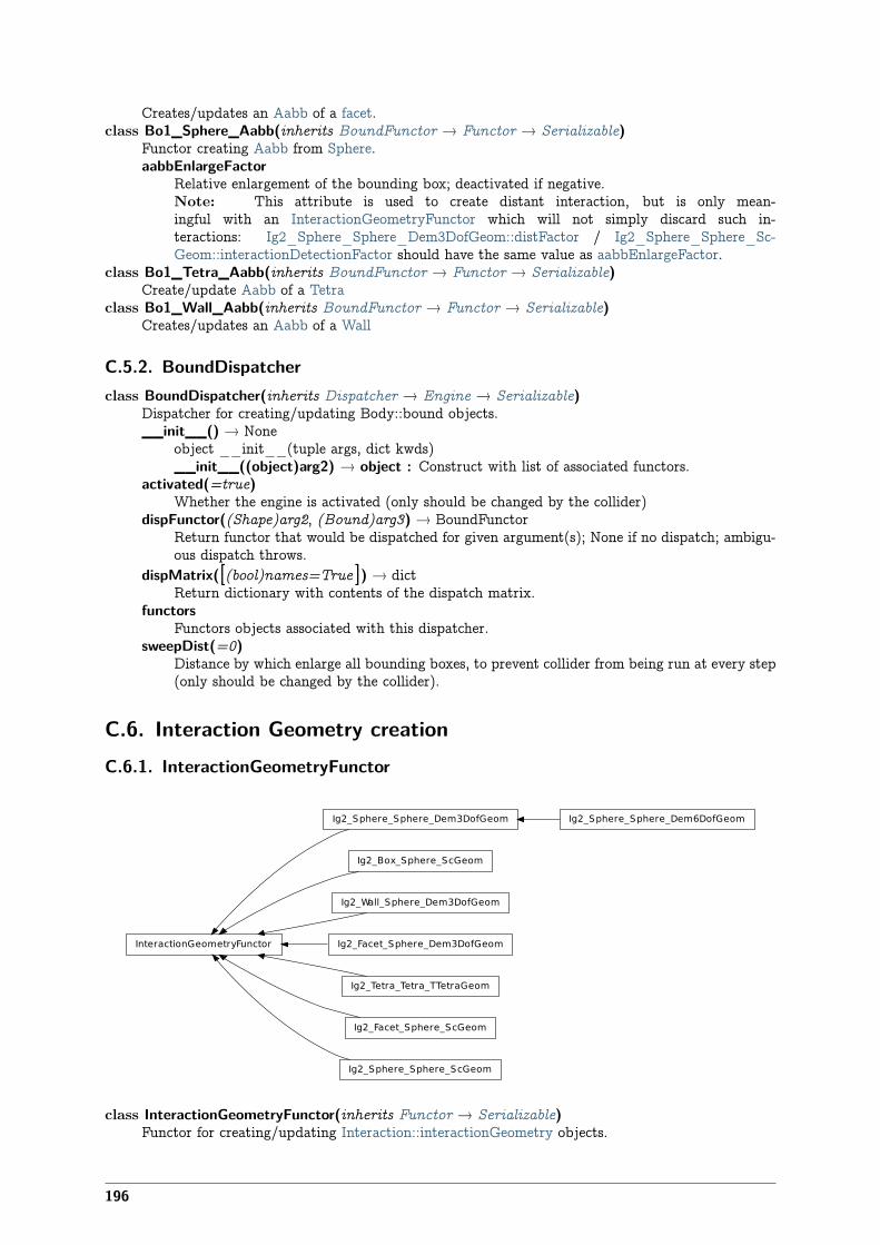
Creates/updates an Aabb of a facet.class Bo1_Sphere_Aabb(inherits BoundFunctor → Functor → Serializable)

Functor creating Aabb from Sphere.aabbEnlargeFactor

Relative enlargement of the bounding box; deactivated if negative.Note: This attribute is used to create distant interaction, but is only mean-ingful with an InteractionGeometryFunctor which will not simply discard such in-teractions: Ig2_Sphere_Sphere_Dem3DofGeom::distFactor / Ig2_Sphere_Sphere_Sc-Geom::interactionDetectionFactor should have the same value as aabbEnlargeFactor.

class Bo1_Tetra_Aabb(inherits BoundFunctor → Functor → Serializable)Create/update Aabb of a Tetra

class Bo1_Wall_Aabb(inherits BoundFunctor → Functor → Serializable)Creates/updates an Aabb of a Wall

C.5.2. BoundDispatcherclass BoundDispatcher(inherits Dispatcher → Engine → Serializable)

Dispatcher for creating/updating Body::bound objects.__init__() → None

object __init__(tuple args, dict kwds)__init__((object)arg2) → object : Construct with list of associated functors.

activated(=true)Whether the engine is activated (only should be changed by the collider)

dispFunctor((Shape)arg2, (Bound)arg3) → BoundFunctorReturn functor that would be dispatched for given argument(s); None if no dispatch; ambigu-ous dispatch throws.

dispMatrix([(bool)names=True ]) → dictReturn dictionary with contents of the dispatch matrix.

functorsFunctors objects associated with this dispatcher.

sweepDist(=0)Distance by which enlarge all bounding boxes, to prevent collider from being run at every step(only should be changed by the collider).

C.6. Interaction Geometry creationC.6.1. InteractionGeometryFunctor

InteractionGeometryFunctor

Ig2_Sphere_Sphere_Dem3DofGeom

Ig2_Box_Sphere_ScGeom

Ig2_Wall_Sphere_Dem3DofGeom

Ig2_Facet_Sphere_Dem3DofGeom

Ig2_Sphere_Sphere_Dem6DofGeom

Ig2_Tetra_Tetra_TTetraGeom

Ig2_Facet_Sphere_ScGeom

Ig2_Sphere_Sphere_ScGeom

class InteractionGeometryFunctor(inherits Functor → Serializable)Functor for creating/updating Interaction::interactionGeometry objects.

196

class Ig2_Box_Sphere_ScGeom(inherits InteractionGeometryFunctor → Functor → Serial-izable)

Create an interaction geometry ScGeom from Box and Sphereclass Ig2_Facet_Sphere_Dem3DofGeom(inherits InteractionGeometryFunctor→ Functor→

Serializable)Compute geometry of facet-sphere contact with normal and shear DOFs. As in all otherDem3DofGeom-related classes, total formulation of both shear and normal deformations is used.See Dem3DofGeom_FacetSphere for more information.

class Ig2_Facet_Sphere_ScGeom(inherits InteractionGeometryFunctor → Functor → Seri-alizable)

Create/update a ScGeom instance representing intersection of Facet and Sphere.shrinkFactor(=0, no shrinking)

The radius of the inscribed circle of the facet is decreased by the value of the sphere’s ra-dius multipled by shrinkFactor. From the definition of contact point on the surface madeof facets, the given surface is not continuous and becomes in effect surface covered with tri-angular tiles, with gap between the separate tiles equal to the sphere’s radius multiplied by2×*shrinkFactor*. If zero, no shrinking is done.

class Ig2_Sphere_Sphere_Dem3DofGeom(inherits InteractionGeometryFunctor → Functor→ Serializable)Functor handling contact of 2 spheres, producing Dem3DofGeom instancedistFactor(=-1)

Factor of sphere radius such that sphere “touch” if their centers are not further than distFac-tor*(r1+r2); if negative, equilibrium distance is the sum of the sphere’s radii.

class Ig2_Sphere_Sphere_Dem6DofGeom(inherits Ig2_Sphere_Sphere_Dem3DofGeom →InteractionGeometryFunctor → Functor → Seri-alizable)

Create/update contact of 2 spheres with 6 DOFs (Dem6DofGeom_SphereSphere instance) [exper-imental]

class Ig2_Sphere_Sphere_ScGeom(inherits InteractionGeometryFunctor → Functor → Se-rializable)

Create/update a ScGeom instance representing intersection of two Spheres.interactionDetectionFactor

Enlarge both radii by this factor (if >1), to permit creation of distant interactions.InteractionGeometry will be computed when interactionDetectionFactor*(rad1+rad2) > dis-tance.Note: This parameter is functionally coupled with Bo1_Sphere_Aabb::aabbEnlargeFactor,which will create larger bounding boxes and should be of the same value.

Warning: Functionally equal class Ig2_Sphere_Sphere_Dem3DofGeom (which createsDem3DofGeom rather than ScGeom) calls this parameter distFactor, but its semantics isdifferent in some aspects.

class Ig2_Tetra_Tetra_TTetraGeom(inherits InteractionGeometryFunctor → Functor → Se-rializable)

Create/update geometry of collision between 2 tetrahedra (TTetraGeom instance)class Ig2_Wall_Sphere_Dem3DofGeom(inherits InteractionGeometryFunctor → Functor →

Serializable)Create/update contact of Wall and Sphere (Dem3DofGeom_WallSphere instance)

C.6.2. InteractionGeometryDispatcherclass InteractionGeometryDispatcher(inherits Dispatcher → Engine → Serializable)

Dispatcher for creating/updating Interaction::interactionGeometry objects__init__() → None

object __init__(tuple args, dict kwds)__init__((object)arg2) → object : Construct with list of associated functors.

dispFunctor((Shape)arg2, (Shape)arg3) → InteractionGeometryFunctorReturn functor that would be dispatched for given argument(s); None if no dispatch; ambigu-ous dispatch throws.

dispMatrix([(bool)names=True ]) → dict

197

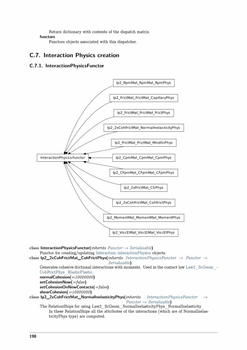
Return dictionary with contents of the dispatch matrix.functors

Functors objects associated with this dispatcher.

C.7. Interaction Physics creationC.7.1. InteractionPhysicsFunctor

InteractionPhys icsFunctor

Ip2_RpmMat_RpmMat_RpmPhys

Ip2_FrictMat_FrictMat_CapillaryPhys

Ip2_FrictMat_FrictMat_FrictPhys

Ip2_2xCohFrictMat_NormalInelasticityPhys

Ip2_FrictMat_FrictMat_MindlinPhys

Ip2_CpmMat_CpmMat_CpmPhys

Ip2_CFpmMat_CFpmMat_CFpmPhys

Ip2_2xFrictMat_CSPhys

Ip2_2xCohFrictMat_CohFrictPhys

Ip2_MomentMat_MomentMat_MomentPhys

Ip2_ViscElMat_ViscElMat_ViscElPhys

class InteractionPhysicsFunctor(inherits Functor → Serializable)Functor for creating/updating Interaction::interactionPhysics objects.

class Ip2_2xCohFrictMat_CohFrictPhys(inherits InteractionPhysicsFunctor → Functor →Serializable)

Generates cohesive-frictional interactions with moments. Used in the contact law Law2_ScGeom_-CohFrictPhys_ElasticPlastic.normalCohesion(=10000000)setCohesionNow(=false)setCohesionOnNewContacts(=false)shearCohesion(=10000000)

class Ip2_2xCohFrictMat_NormalInelasticityPhys(inherits InteractionPhysicsFunctor →Functor → Serializable)

The RelationShips for using Law2_ScGeom_NormalInelasticityPhys_NormalInelasticityIn these RelationShips all the attributes of the interactions (which are of NormalInelas-ticityPhys type) are computed.

198

Warning: as in the others Ip2 functors, most of the attributes are computed only once, whenthe interaction is new.

betaR(=0.12)Parameter for computing the torque-stifness : T-stifness = betaR * Rmoy^2

setCohesionNow(=false)setCohesionOnNewContacts(=false)

class Ip2_2xFrictMat_CSPhys(inherits InteractionPhysicsFunctor→ Functor→ Serializable)Functor creating CSPhys from two FrictMat. See Law2_Dem3Dof_CSPhys_CundallStrack fordetails.

class Ip2_CFpmMat_CFpmMat_CFpmPhys(inherits InteractionPhysicsFunctor → Functor→ Serializable)Converts 2 CFpmmat instances to CFpmPhys with corresponding parameters.Alpha(=0)

Defines the ratio ks/kn.Beta(=0)

Defines the ratio kr/(ks*meanRadius^2) to compute the resistive moment in rotation. [-]cohesion(=0)

Defines the maximum admissible tangential force in shear FsMax=cohesion*crossSection. [Pa]cohesiveTresholdIteration(=1)

Should new contacts be cohesive? They will before this iter, they won’t afterward.eta(=0)

Defines the maximum admissible resistive moment in rotation MtMax=eta*meanRadius*Fn.[-]

strengthSoftening(=0)Defines the softening when Dtensile is reached to avoid explosion of the contact. Typically,when D > Dtensile, Fn=FnMax - (kn/strengthSoftening)*(Dtensile-D). [-]

tensileStrength(=0)Defines the maximum admissible normal force in traction Fn-Max=tensileStrength*crossSection. [Pa]

useAlphaBeta(=false)If true, stiffnesses are computed based on Alpha and Beta.

class Ip2_CpmMat_CpmMat_CpmPhys(inherits InteractionPhysicsFunctor → Functor →Serializable)

Convert 2 CpmMat instances to CpmPhys with corresponding parameters. Uses simple (arithmetic)averages if material are different. Simple copy of parameters is performed if the material is sharedbetween both particles. See cpm-model for detals.cohesiveThresholdIter(=10)

Should new contacts be cohesive? They will before this iter#, they will not be afterwards. If0, they will never be. If negative, they will always be created as cohesive (10 by default).

class Ip2_FrictMat_FrictMat_CapillaryPhys(inherits InteractionPhysicsFunctor → Functor→ Serializable)RelationShips to use with Law2_ScGeom_CapillaryPhys_Capillarity

In these RelationShips all the interaction attributes are computed.Warning: as in the others Ip2 functors, most of the attributes are computed only once, whenthe interaction is new.

class Ip2_FrictMat_FrictMat_FrictPhys(inherits InteractionPhysicsFunctor → Functor →Serializable)

Create a FrictPhys from two FrictMats. The compliance of one sphere under symetric point loadsis defined here as 1/(E.r), with E the stiffness of the sphere and r its radius, and corresponds to acompliance 1/(2.E.r)=1/(E.D) from each contact point. The compliance of the contact itself willbe the sum of compliances from each sphere, i.e. 1/(E.D1)+1/(E.D2) in the general case, or 1/(E.r)in the special case of equal sizes. Note that summing compliances corresponds to an harmonic av-erage of stiffnesss, which is how kn is actually computed in the Ip2_FrictMat_FrictMat_FrictPhysfunctor.

The shear stiffness ks of one sphere is defined via the material parameter Frict-Phys::poisson, as ks=poisson*kn, and the resulting shear stiffness of the interaction will

199

be also an harmonic average.The friction angle of the contact is defined as the minimum angle of the two materials incontact.

Only interactions with ScGeom or Dem3DofGeom geometry are meaningfully accepted; run-timetypecheck can make this functor unnecessarily slow in general. Such design is problematic in itself,though – from http://www.mail-archive.com/yade-dev@lists.launchpad.net/msg02603.html:

You have to suppose some exact type of InteractionGeometry in the Ip2 functor, but youdon’t know anything about it (Ip2 only guarantees you get certain InteractionPhysicstypes, via the dispatch mechanism).That means, unless you use Ig2 functor producing the desired type, the code will break(crash or whatever). The right behavior would be either to accept any type (what we havenow, at least in principle), or really enforce InteractionGeometry type of the interationpassed to that particular Ip2 functor.

Etc.class Ip2_FrictMat_FrictMat_MindlinPhys(inherits InteractionPhysicsFunctor→ Functor→

Serializable)Calculate some physical parameters needed to obtain the normal and shear stiffnesses according tothe Hertz-Mindlin’s formulation (as implemented in PFC).

class Ip2_MomentMat_MomentMat_MomentPhys(inherits InteractionPhysicsFunctor →Functor → Serializable)

Create MomentPhys from 2 instances of MomentMat.1.If boolean userInputStiffness=true & useAlphaBeta=false, users can input Knormal, Kshearand Krotate directly. Then, kn,ks and kr will be equal to these values, rather than calculatedE and v.

2.If boolean userInputStiffness=true & useAlphaBeta=true, users input Knormal, Alpha andBeta. Then ks and kr are calculated from alpha & beta respectively.

3.If both are false, it calculates kn and ks are calculated from E and v, whilst kr = 0.Alpha(=0)

Ratio of Ks/KnBeta(=0)

Ratio to calculate KrKnormal(=0)

Allows user to input stiffness properties from triaxial test. These will be passed to MomentPhysor NormShearPhys

Krotate(=0)Allows user to input stiffness properties from triaxial test. These will be passed to MomentPhysor NormShearPhys

Kshear(=0)Allows user to input stiffness properties from triaxial test. These will be passed to MomentPhysor NormShearPhys

useAlphaBeta(=false)for users to choose whether to input stiffness directly or use ratios to calculate Ks/Kn

userInputStiffness(=false)for users to choose whether to input stiffness directly or use ratios to calculate Ks/Kn

class Ip2_RpmMat_RpmMat_RpmPhys(inherits InteractionPhysicsFunctor → Functor →Serializable)

Convert 2 RpmMat instances to RpmPhys with corresponding parameters.initDistance(=0)

Initial distance between spheres at the first step.class Ip2_ViscElMat_ViscElMat_ViscElPhys(inherits InteractionPhysicsFunctor → Functor→ Serializable)

Convert 2 instances of ViscElMat to ViscElPhys using the rule of consecutive connection.

C.7.2. InteractionPhysicsDispatcherclass InteractionPhysicsDispatcher(inherits Dispatcher → Engine → Serializable)

Dispatcher for creating/updating Interaction::interactionPhysics objects.__init__() → None

object __init__(tuple args, dict kwds)

200

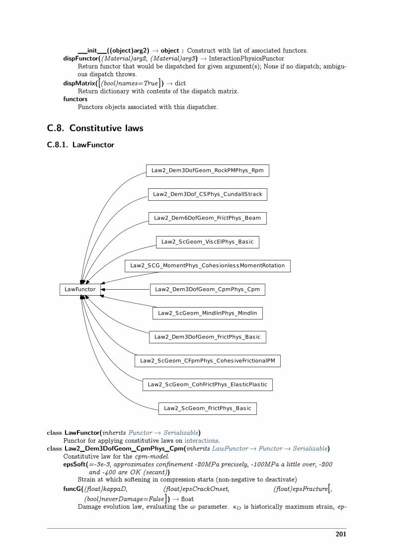
__init__((object)arg2) → object : Construct with list of associated functors.dispFunctor((Material)arg2, (Material)arg3) → InteractionPhysicsFunctor

Return functor that would be dispatched for given argument(s); None if no dispatch; ambigu-ous dispatch throws.

dispMatrix([(bool)names=True ]) → dictReturn dictionary with contents of the dispatch matrix.

functorsFunctors objects associated with this dispatcher.

C.8. Constitutive lawsC.8.1. LawFunctor

LawFunctor

Law2_Dem3DofGeom_RockPMPhys_Rpm

Law2_Dem3Dof_CSPhys_CundallStrack

Law2_Dem6DofGeom_FrictPhys_Beam

Law2_ScGeom_ViscElPhys_Bas ic

Law2_SCG_MomentPhys_Cohes ionles sMomentRotation

Law2_Dem3DofGeom_CpmPhys_Cpm

Law2_ScGeom_MindlinPhys_Mindlin

Law2_Dem3DofGeom_FrictPhys_Bas ic

Law2_ScGeom_CFpmPhys_Cohes iveFrictionalPM

Law2_ScGeom_CohFrictPhys_ElasticPlastic

Law2_ScGeom_FrictPhys_Bas ic

class LawFunctor(inherits Functor → Serializable)Functor for applying constitutive laws on interactions.

class Law2_Dem3DofGeom_CpmPhys_Cpm(inherits LawFunctor→ Functor→ Serializable)Constitutive law for the cpm-model.epsSoft(=-3e-3, approximates confinement -20MPa precisely, -100MPa a little over, -200

and -400 are OK (secant))Strain at which softening in compression starts (non-negative to deactivate)

funcG((float)kappaD, (float)epsCrackOnset, (float)epsFracture[,(bool)neverDamage=False ]) → float

Damage evolution law, evaluating the ω parameter. κD is historically maximum strain, ep-

201

sCrackOnset (ε0) = CpmMat.epsCrackOnset, epsFracture = CpmMat.epsFracture; if never-Damage is True, the value returned will always be 0 (no damage).

omegaThreshold(=1., >=1. to deactivate, i.e. never delete any contacts)damage after which the contact disappears (<1), since omega reaches 1 only for strain →+∞

relKnSoft(=.3)Relative rigidity of the softening branch in compression (0=perfect elastic-plastic, <0 soften-ing, >0 hardening)

yieldEllipseShift(=NaN)horizontal scaling of the ellipse (shifts on the +x axis as interactions with +y are given)

yieldLogSpeed(=.1)scaling in the logarithmic yield surface (should be <1 for realistic results; >=0 for meaningfulresults)

yieldSigmaTMagnitude((float)sigmaN, (float)omega, (float)undamagedCohesion,(float)tanFrictionAngle) → float

Return radius of yield surface for given material and state parameters; uses attributes of thecurrent instance (yieldSurfType etc), change them before calling if you need that.

yieldSurfType(=2)yield function: 0: mohr-coulomb (original); 1: parabolic; 2: logarithmic, 3: log+lin_tension,4: elliptic, 5: elliptic+log

class Law2_Dem3DofGeom_FrictPhys_Basic(inherits LawFunctor → Functor → Serializ-able)

Constitutive law for linear compression, no tension, and linear plasticity surface.This class serves also as tutorial and is documented in detail at https://yade-dem.org/index.php/ConstitutiveLawHowto.

class Law2_Dem3DofGeom_RockPMPhys_Rpm(inherits LawFunctor → Functor → Serial-izable)

Constitutive law for the Rpm modelclass Law2_Dem3Dof_CSPhys_CundallStrack(inherits LawFunctor → Functor → Serializ-

able)Basic constitutive law published originally by Cundall&Strack; it has normal and shear stiffnesses(Kn, Kn) and dry Coulomb friction. Operates on associated Dem3DofGeom and CSPhys instances.

class Law2_Dem6DofGeom_FrictPhys_Beam(inherits LawFunctor → Functor → Serializ-able)

Class for demonstrating beam-like behavior of contact (normal, shear, bend and twist) [bro-ken][experimental]

class Law2_SCG_MomentPhys_CohesionlessMomentRotation(inherits LawFunctor → Func-tor → Serializable)

Contact law based on Plassiard et al. (2009) : A spherical discrete element model: calibrationprocedure and incremental response. The functionality has been verified with results in the paper.The contribution of stiffnesses are scaled according to the radius of the particle, as implemented inthat paper.See also associated classes MomentMat, Ip2_MomentMat_MomentMat_MomentPhys, Moment-Phys.Note: This constitutive law can be used with triaxial test, but the following significant changes incode have to be made: Ip2_MomentMat_MomentMat_MomentPhys and Law2_SCG_Moment-Phys_CohesionlessMomentRotation have to be added. Since it uses ScGeom, it uses boxes ratherthan facets. Spheres and boxes have to be changed to MomentMat rather than FrictMat.preventGranularRatcheting(=false)

??class Law2_ScGeom_CFpmPhys_CohesiveFrictionalPM(inherits LawFunctor → Functor →

Serializable)Constitutive law for the CFpm model.preventGranularRatcheting(=false)

If true rotations are computed such as granular ratcheting is prevented. See article [2], pg.3-10 – and a lot more papers from the same authors).

class Law2_ScGeom_CohFrictPhys_ElasticPlastic(inherits LawFunctor → Functor → Serial-izable)

Law for linear traction-compression-bending-twisting, with cohesion+friction and Mohr-Coulombplasticity surface. Can be elastic-fragile or perfectly elastic-plastic. Creep at contact can be enabled.

202

Note: This law uses ScGeom.always_use_moment_law(=false)

If true, use bending/twisting moments at all contacts. If false, compute moments only forcohesive contacts.

creep_viscosity(=1)creep viscosity [Pa.s/m]. probably should be moved to Ip2_2xCohFrictMat_CohFrictPhys...

detectBrokenBodies(=false)erosionActivated(=false)momentRotationLaw(=false)

use bending/twisting moment at contacts. See CohesiveFrictionalContactLaw::always_use_-moment_law for details.

neverErase(=false)Keep interactions even if particles go away from each other (only in case another constitutivelaw is in the scene, e.g. Law2_ScGeom_CapillaryPhys_Capillarity)

shear_creep(=false)activate creep on the shear force, using CohesiveFrictionalContactLaw::creep_viscosity.

twist_creep(=false)activate creep on the twisting moment, using CohesiveFrictionalContactLaw::creep_viscosity.

class Law2_ScGeom_FrictPhys_Basic(inherits LawFunctor → Functor → Serializable)Law for linear compression, without cohesion and Mohr-Coulomb plasticity surface.Note: This law uses ScGeom; there is also functionally equivalent Law2_Dem3DofGeom_-FrictPhys_Basic, which uses Dem3DofGeom (sphere-box interactions are not implemented for thelatest).elasticEnergy() → float

Compute and return the total elastic energy in all “FrictPhys” contactsinitPlasticDissipation((float)arg2) → None

Initialize cummulated plastic dissipation to a value (0 by default).neverErase(=false)

Keep interactions even if particles go away from each other (only in case another constitutivelaw is in the scene, e.g. Law2_ScGeom_CapillaryPhys_Capillarity)

plasticDissipation() → floatTotal energy dissipated in plastic slips at all FrictPhys contacts. Computed only if Law2_-ScGeom_FrictPhys_Basic::traceEnergy is true.

traceEnergy(=false)Define the total energy dissipated in plastic slips at all contacts.

useShear(=false)Use ScGeom::updateShear rather than ScGeom::rotateAndGetShear for shear force computa-tion.

class Law2_ScGeom_MindlinPhys_Mindlin(inherits LawFunctor → Functor → Serializable)Constitutive law for the Mindlin’s formulation.preventGranularRatcheting(=false)

bool to avoid granular ratchetingclass Law2_ScGeom_ViscElPhys_Basic(inherits LawFunctor → Functor → Serializable)

Linear viscoelastic model operating on ScGeom and ViscElPhys.

C.8.2. LawDispatcherclass LawDispatcher(inherits Dispatcher → Engine → Serializable)

Dispatcher for applying constitutive laws on interactions.__init__() → None

object __init__(tuple args, dict kwds)__init__((object)arg2) → object : Construct with list of associated functors.

dispFunctor((InteractionGeometry)arg2, (InteractionPhysics)arg3) → LawFunctorReturn functor that would be dispatched for given argument(s); None if no dispatch; ambigu-ous dispatch throws.

dispMatrix([(bool)names=True ]) → dictReturn dictionary with contents of the dispatch matrix.

functors

203

Functors objects associated with this dispatcher.

C.9. CallbacksC.9.1. BodyCallback

BodyCallback SumBodyForcesCb

class BodyCallback(inherits Serializable)Abstract callback object which will be called for every Body after being processed by NewtonInte-grator. See IntrCallback for details.

class SumBodyForcesCb(inherits BodyCallback → Serializable)Callback summing magnitudes of resultant forces over dynamic bodies.

C.9.2. IntrCallback

IntrCallback SumIntrForcesCb

class IntrCallback(inherits Serializable)Abstract callback object which will be called for every (real) Interaction after the interaction hasbeen processed by InteractionDispatchers.At the beginning of the interaction loop, stepInit is called, initializing the object; it returns eitherNULL (to deactivate the callback during this time step) or pointer to function, which will then bepassed (1) pointer to the callback object itself and (2) pointer to Interaction.Note: (NOT YET DONE) This functionality is accessible from python by passing 4th argumentto InteractionDispatchers constructor, or by appending the callback object to InteractionDispatch-ers::callbacks.

class SumIntrForcesCb(inherits IntrCallback → Serializable)Callback summing magnitudes of forces over all interactions. InteractionPhysics of interactionsmust derive from NormShearPhys (responsability fo the user).

C.10. Preprocessors

FileGenerator

TriaxialTestWater

TriaxialTest

class FileGenerator(inherits Serializable)Base class for scene generators, preprocessors.generate((str)out) → None

Generate scene, save to given fileload() → None

Generate scene, save to temporary file and load immediatelyoutputFileName(=”./scene.xml” )

Filename to write resulting simulation toclass TriaxialTest(inherits FileGenerator → Serializable)

Prepare a scene for triaxial tests. See full documentation at http://yade-dem.org/wiki/TriaxialTest.

204

Key(=”“)A code that is added to output filenames.

StabilityCriterion(=0.01)Value of unbalanced force for which the system is considered stable. Used in conditionals toswitch between loading stages.

WallStressRecordFile(=”./WallStresses”+Key)autoCompressionActivation(=true)

Do we just want to generate a stable packing under isotropic pressure (false) or do we wantthe triaxial loading to start automatically right after compaction stage (true)?

autoStopSimulation(=false)freeze the simulation when conditions are reached (don’t activate this if you want to be ableto run/stop from Qt GUI)

autoUnload(=true)auto adjust the isotropic stress state from TriaxialTest::sigmaIsoCompaction to Triaxial-Test::sigmaLateralConfinement if they have different values. See docs for TriaxialCompressio-nEngine::autoUnload

biaxial2dTest(=false)FIXME : what is that?

boxFrictionDeg(=0.0)Friction angle [°] of boundaries contacts.

boxKsDivKn(=0.5)Ratio of shear vs. normal contact stiffness for boxes.

boxWalls(=true)Use boxes for boundaries (recommended).

boxYoungModulus(=15000000.0)Stiffness of boxes.

compactionFrictionDeg(=sphereFrictionDeg)Friction angle [°] of spheres during compaction (different values result in different porosities)].This value is overriden by TriaxialTest::sphereFrictionDeg before triaxial testing.

dampingForce(=0.2)Coefficient of Cundal-Non-Viscous damping (applied on on the 3 components of forces)

dampingMomentum(=0.2)Coefficient of Cundal-Non-Viscous damping (applied on on the 3 components of torques)

defaultDt(=-1)Max time-step. Used as initial value if defined. Latter adjusted by the time stepper.

density(=2600)density of spheres

facetWalls(=false)Use facets for boundaries (not tested)

finalMaxMultiplier(=1.001)max multiplier of diameters during internal compaction (secondary precise adjustment)

fixedBoxDims(=”“)string that contains some subset (max. 2) of {‘x’,’y’,’z’} ; containes axes will have box dimen-sion hardcoded, even if box is scaled as mean_radius is prescribed: scaling will be applied onthe rest.

fixedPoroCompaction(=false)flag to choose an isotropic compaction until a fixed porosity choosing a same translation speedfor the six walls

fixedPorosity(=1)FIXME : what is that?

importFilename(=”“)File with positions and sizes of spheres.

internalCompaction(=false)flag for choosing between moving boundaries or increasing particles sizes during the compactionstage.

lowerCorner(=Vector3r(0, 0, 0))Lower corner of the box.

maxMultiplier(=1.01)

205

max multiplier of diameters during internal compaction (initial fast increase)maxWallVelocity(=10)

max velocity of boundaries. Usually useless, but can help stabilizing the system in some cases.noFiles(=false)

Do not create any files during run (.xml, .spheres, wall stress records)numberOfGrains(=400)

Number of generated spheres.radiusControlInterval(=10)

interval between size changes when growing spheres.radiusMean(=-1)

Mean radius. If negative (default), autocomputed to as a function of box size and Triaxial-Test::numberOfGrains

radiusStdDev(=0.3)Normalized standard deviation of generated sizes.

recordIntervalIter(=20)interval between file outputs

sigmaIsoCompaction(=50000)Confining stress during isotropic compaction.

sigmaLateralConfinement(=50000)Lateral stress during triaxial loading. An isotropic unloading is performed if the value is notequal to TriaxialTest::SigmaIsoCompaction.

sphereFrictionDeg(=18.0)Friction angle [°] of spheres assigned just before triaxial testing.

sphereKsDivKn(=0.5)Ratio of shear vs. normal contact stiffness for spheres.

sphereYoungModulus(=15000000.0)Stiffness of spheres.

strainRate(=0.1)Strain rate in triaxial loading.

thickness(=0.001)thickness of boundaries. It is arbitrary and should have no effect

timeStepUpdateInterval(=50)interval for GlobalStiffnessTimeStepper

upperCorner(=Vector3r(1, 1, 1))Upper corner of the box.

wallOversizeFactor(=1.3)Make boundaries larger than the packing to make sure spheres don’t go out during deformation.

wallStiffnessUpdateInterval(=10)interval for updating the stiffness of sample/boundaries contacts

wallWalls(=false)Use walls for boundaries (not tested)

class TriaxialTestWater(inherits FileGenerator → Serializable)This preprocessor is a variant of TriaxialTest, including the model of capillary forces developpedas part of the PhD of Luc Scholtès. See the documentation of Law2_ScGeom_CapillaryPhys_-Capillarity or the main page https://yade-dem.org/wiki/CapillaryTriaxialTest, for more details.Results obtained with this preprocessor were reported for instance in ‘Scholtes et al. Microme-chanics of granular materials with capillary effects. International Journal of Engineering Science2009,(47)1, 64-75.’CapillaryPressure(=0)

Define succion in the packing [Pa]. This is the value used in the capillary model.Key(=”“)

A code that is added to output filenames.Rdispersion(=0.3)

Normalized standard deviation of generated sizes.StabilityCriterion(=0.01)

Value of unbalanced force for which the system is considered stable. Used in conditionals toswitch between loading stages.

WallStressRecordFile(=”./WallStressesWater”+Key)

206

autoCompressionActivation(=true)Do we just want to generate a stable packing under isotropic pressure (false) or do we wantthe triaxial loading to start automatically right after compaction stage (true)?

autoStopSimulation(=false)freeze the simulation when conditions are reached (don’t activate this if you want to be ableto run/stop from Qt GUI)

autoUnload(=true)auto adjust the isotropic stress state from TriaxialTest::sigmaIsoCompaction to Triaxial-Test::sigmaLateralConfinement if they have different values. See docs for TriaxialCompressio-nEngine::autoUnload

biaxial2dTest(=false)FIXME : what is that?

binaryFusion(=true)Defines how overlapping bridges affect the capillary forces (see TriaxialTestWa-ter::fusionDetection). If binary=true, the force is null as soon as there is an overlap detected,if not, the force is divided by the number of overlaps.

boxFrictionDeg(=0.0)Friction angle [°] of boundaries contacts.

boxKsDivKn(=0.5)Ratio of shear vs. normal contact stiffness for boxes.

boxWalls(=true)Use boxes for boundaries (recommended).

boxYoungModulus(=15000000.0)Stiffness of boxes.

capillaryStressRecordFile(=”./capStresses”+Key)compactionFrictionDeg(=sphereFrictionDeg)

Friction angle [°] of spheres during compaction (different values result in different porosities)].This value is overriden by TriaxialTest::sphereFrictionDeg before triaxial testing.

contactStressRecordFile(=”./contStresses”+Key)dampingForce(=0.2)

Coefficient of Cundal-Non-Viscous damping (applied on on the 3 components of forces)dampingMomentum(=0.2)

Coefficient of Cundal-Non-Viscous damping (applied on on the 3 components of torques)defaultDt(=0.0001)

Max time-step. Used as initial value if defined. Latter adjusted by the time stepper.density(=2600)

density of spheresfacetWalls(=false)

Use facets for boundaries (not tested)finalMaxMultiplier(=1.001)

max multiplier of diameters during internal compaction (secondary precise adjustment)fixedBoxDims(=”“)

string that contains some subset (max. 2) of {‘x’,’y’,’z’} ; containes axes will have box dimen-sion hardcoded, even if box is scaled as mean_radius is prescribed: scaling will be applied onthe rest.

fixedPoroCompaction(=false)flag to choose an isotropic compaction until a fixed porosity choosing a same translation speedfor the six walls

fixedPorosity(=1)FIXME : what is that?

fusionDetection(=false)test overlaps between liquid bridges on modify forces if overlaps exist

importFilename(=”“)File with positions and sizes of spheres.

internalCompaction(=false)flag for choosing between moving boundaries or increasing particles sizes during the compactionstage.

lowerCorner(=Vector3r(0, 0, 0))

207

Lower corner of the box.maxMultiplier(=1.01)

max multiplier of diameters during internal compaction (initial fast increase)maxWallVelocity(=10)

max velocity of boundaries. Usually useless, but can help stabilizing the system in some cases.noFiles(=false)

Do not create any files during run (.xml, .spheres, wall stress records)numberOfGrains(=400)

Number of generated spheres.radiusControlInterval(=10)

interval between size changes when growing spheres.radiusMean(=-1)

Mean radius. If negative (default), autocomputed to as a function of box size and Triaxial-Test::numberOfGrains

recordIntervalIter(=20)interval between file outputs

sigmaIsoCompaction(=50000)Confining stress during isotropic compaction.

sigmaLateralConfinement(=50000)Lateral stress during triaxial loading. An isotropic unloading is performed if the value is notequal to TriaxialTestWater::SigmaIsoCompaction.

sphereFrictionDeg(=18.0)Friction angle [°] of spheres assigned just before triaxial testing.

sphereKsDivKn(=0.5)Ratio of shear vs. normal contact stiffness for spheres.

sphereYoungModulus(=15000000.0)Stiffness of spheres.

strainRate(=1)Strain rate in triaxial loading.

thickness(=0.001)thickness of boundaries. It is arbitrary and should have no effect

timeStepOutputInterval(=50)interval for outputing general informations on the simulation (stress,unbalanced force,...)

timeStepUpdateInterval(=50)interval for GlobalStiffnessTimeStepper

upperCorner(=Vector3r(1, 1, 1))Upper corner of the box.

wallOversizeFactor(=1.3)Make boundaries larger than the packing to make sure spheres don’t go out during deformation.

wallStiffnessUpdateInterval(=10)interval for updating the stiffness of sample/boundaries contacts

wallWalls(=false)Use walls for boundaries (not tested)

water(=true)activate capillary model

C.11. RenderingC.11.1. OpenGLRenderingEngineclass OpenGLRenderingEngine(inherits Serializable)

Class responsible for rendering scene on OpenGL devices.bgColor(=Vector3r(.2, .2, .2))

Color of the backgroud canvas (RGB)bound(=false)

Render body BoundclipPlaneActive(=vector<int>(numClipPlanes, 0))

Activate/deactivate respective clipping planes

208

clipPlaneSe3(=vector<Se3r>(numClipPlanes, Se3r(Vector3r::Zero(), Quater-nionr::Identity())))

Position and orientation of clipping planesdispScale(=Vector3r::Ones(), disable scaling)

Artificially enlarge (scale) dispalcements from bodies’ reference positions by this relativeamount, so that they become better visible (independently in 3 dimensions). Disbled if (1,1,1).

dof(=false)Show which degrees of freedom are blocked for each body

id(=false)Show body id’s

intrAllWire(=false)Draw wire for all interactions, blue for potential and green for real ones (mostly for debugging)

intrGeom(=false)Render Interaction::interactionGeometry objects.

intrPhys(=false)Render Interaction::interactionPhysics objects

intrWire(=false)If rendering interactions, use only wires to represent them.

lightPos(=Vector3r(75, 130, 0))Position of OpenGL light source in the scene.

mask(=~0, draw everything)Bitmask for showing only bodies where ((mask & Body::mask)!=0)

rotScale(=1., disable scaling)Artificially enlarge (scale) rotations of bodies relative to their reference orientation, so thethey are better visible.

selectBodyLimit(=1000)Limit number of bodies to allow picking body with mouse (performance reasons)

setRefSe3() → NoneMake current positions and orientation reference for scaleDisplacements and scaleRotations.

shape(=true)Render body Shape

wire(=false)Render all bodies with wire only (faster)

C.11.2. GlShapeFunctor

GlShapeFunctor

Gl1_Sphere

Gl1_Tetra

Gl1_Box

Gl1_Wall

Gl1_Facet

class GlShapeFunctor(inherits Functor → Serializable)Abstract functor for rendering Body::shape objects.

class Gl1_Box(inherits GlShapeFunctor → Functor → Serializable)Renders Box object

class Gl1_Facet(inherits GlShapeFunctor → Functor → Serializable)Renders Facet object

209

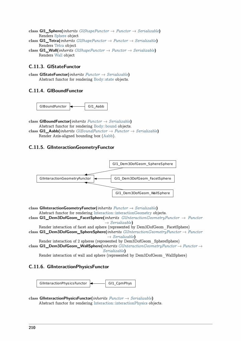
class Gl1_Sphere(inherits GlShapeFunctor → Functor → Serializable)Renders Sphere object

class Gl1_Tetra(inherits GlShapeFunctor → Functor → Serializable)Renders Tetra object

class Gl1_Wall(inherits GlShapeFunctor → Functor → Serializable)Renders Wall object

C.11.3. GlStateFunctorclass GlStateFunctor(inherits Functor → Serializable)

Abstract functor for rendering Body::state objects.

C.11.4. GlBoundFunctor

GlBoundFunctor Gl1_Aabb

class GlBoundFunctor(inherits Functor → Serializable)Abstract functor for rendering Body::bound objects.

class Gl1_Aabb(inherits GlBoundFunctor → Functor → Serializable)Render Axis-aligned bounding box (Aabb).

C.11.5. GlInteractionGeometryFunctor

GlInteractionGeometryFunctor

Gl1_Dem3DofGeom_SphereSphere

Gl1_Dem3DofGeom_FacetSphere

Gl1_Dem3DofGeom_WallSphere

class GlInteractionGeometryFunctor(inherits Functor → Serializable)Abstract functor for rendering Interaction::interactionGeometry objects.

class Gl1_Dem3DofGeom_FacetSphere(inherits GlInteractionGeometryFunctor → Functor→ Serializable)Render interaction of facet and sphere (represented by Dem3DofGeom_FacetSphere)

class Gl1_Dem3DofGeom_SphereSphere(inherits GlInteractionGeometryFunctor → Functor→ Serializable)Render interaction of 2 spheres (represented by Dem3DofGeom_SphereSphere)

class Gl1_Dem3DofGeom_WallSphere(inherits GlInteractionGeometryFunctor→ Functor→Serializable)

Render interaction of wall and sphere (represented by Dem3DofGeom_WallSphere)

C.11.6. GlInteractionPhysicsFunctor

GlInteractionPhys icsFunctor Gl1_CpmPhys

class GlInteractionPhysicsFunctor(inherits Functor → Serializable)Abstract functor for rendering Interaction::interactionPhysics objects.

210

class Gl1_CpmPhys(inherits GlInteractionPhysicsFunctor → Functor → Serializable)Render CpmPhys objects of interactions.

C.12. Simulation dataC.12.1. Omegaclass Omega

bodiesBodies in the current simulation (container supporting index access by id and iteration)

cellPeriodic cell of the current scene (None if the scene is aperiodic).

childClassesNonrecursive((str)arg2) → listReturn list of all classes deriving from given class, as registered in the class factory

disableGdb() → NoneRevert SEGV and ABRT handlers to system defaults.

dtCurrent timestep (∆t) value.

•assigning zero enables dynamic ∆t control via a TimeStepper (raises an exception if thereis no TimeStepper among O.engines)

•assigning negative value enables dynamic ∆t (as in the previous case) and sets positivetimestep O.dt=|∆t| (will be used until the timestepper is run and updates it)

•assigning positive value sets ∆t to that value and disables dynamic ∆t (via TimeStepper,if there is one).

dynDt can be used to query whether dynamic ∆t is in use.dynDt

Whether a TimeStepper is used for dynamic ∆t control. See dt on how to enable/disableTimeStepper.

enginesList of engines in the simulation (Scene::engines).

exitNoBacktrace([(int)status=0 ]) → NoneDisable SEGV handler and exit, optionally with given status number.

forceSyncCountCounter for number of syncs in ForceContainer, for profiling purposes.

forcesForceContainer (forces, torques, displacements) in the current simulation.

initializersList of initializers (Scene::initializers).

interactionsInteractions in the current simulation (container supporting index acces by either (id1,id2) orinteractionNumber and iteration)

isChildClassOf((str)arg2, (str)arg3) → boolTells whether the first class derives from the second one (both given as strings).

iterGet current step number

labeledEngine((str)arg2) → objectReturn instance of engine/functor with the given label. This function shouldn’t be calledby the user directly; every ehange in O.engines will assign respective global python variablesaccording to labels.For example:: O.engines=[InsertionSortCollider(label=’collider’)] collider.nBins=5 ## col-lider has become a variable after assignment to O.engines automatically)

load((str)arg2) → NoneLoad simulation from file.

load2((str)arg2) → None[EXPERIMENTAL] load using boost::serialization (handles compression, XML/binary)

loadTmp([(str)mark=’‘ ]) → None

211

Load simulation previously stored in memory by saveTmp. mark optionally distinguishesmultiple saved simulations

materialsShared materials; they can be accessed by id or by label

miscParamsMiscParams in the simulation (Scene::mistParams), usually used to save serializables thatdon’t fit anywhere else, like GL functors

numThreadsGet maximum number of threads openMP can use.

pause() → NoneStop simulation execution. (May be called from within the loop, and it will stop after thecurrent step).

periodicGet/set whether the scene is periodic or not (True/False).

plugins() → listReturn list of all plugins registered in the class factory.

realtimeReturn clock (human world) time the simulation has been running.

reload() → NoneReload current simulation

reset() → NoneReset simulations completely (including another scene!).

resetThisScene() → NoneReset current scene.

resetTime() → NoneReset simulation time: step number, virtual and real time. (Doesn’t touch anything else,including timings).

run([(int)nSteps=-1[, (bool)wait=False ] ]) → NoneRun the simulation. nSteps how many steps to run, then stop (if positive); wait will causenot returning to python until simulation will have stopped.

runEngine((Engine)arg2) → NoneRun given engine exactly once; simulation time, step number etc. will not be incremented(use only if you know what you do).

save((str)arg2) → NoneSave current simulation to file (should be .xml or .xml.bz2)

save2((str)arg2) → None[EXPERIMENTAL] save using boost::serialization (handles compression, XML/binary)

saveTmp([(str)mark=’‘ ]) → NoneSave simulation to memory (disappears at shutdown), can be loaded later with loadTmp.mark optionally distinguishes different memory-saved simulations.

step() → NoneAdvance the simulation by one step. Returns after the step will have finished.

stopAtIterGet/set number of iteration after which the simulation will stop.

switchScene() → NoneSwitch to alternative simulation (while keeping the old one). Calling the function againswitches back to the first one. Note that most variables from the first simulation will stillrefer to the first simulation even after the switch (e.g. b=O.bodies[4]; O.switchScene(); [b stillrefers to the body in the first simulation here])

tagsTags (string=string dictionary) of the current simulation (container supporting string-indexaccess/assignment)

timeReturn virtual (model world) time of the simulation.

timingEnabledGlobally enable/disable timing services (see documentation of yade.timing).

tmpFilename() → strReturn unique name of file in temporary directory which will be deleted when yade exits.

212

tmpToFile((str)fileName[, (str)mark=’‘ ]) → NoneSave XML of saveTmp‘d simulation into fileName.

tmpToString([(str)mark=’‘ ]) → strReturn XML of saveTmp‘d simulation as string.

wait() → NoneDon’t return until the simulation will have been paused. (Returns immediately if not running).

C.12.2. BodyContainerclass BodyContainer

__init__((BodyContainer)arg2) → Noneappend((Body)arg2) → int

Append one Body instance, return its id.append( (BodyContainer)arg1, (object)arg2) → object : Append list of Body instance, re-

turn list of idsappendClumped((object)arg2) → tuple

Append given list of bodies as a clump (rigid aggregate); return list of ids.clear() → None

Remove all bodies (interactions not checked)erase((int)arg2) → bool

Erase body with the given id; all interaction will be deleted by InteractionDispatchers in thenext step.

replace((object)arg2) → object

C.12.3. InteractionContainerclass InteractionContainer

Access to interactions of simulation, by using1.id’s of both Bodies of the interactions, e.g. O.interactions[23,65]2.iteraction over the whole container:

for i in O.interactions: print i.id1,i.id2

Note: Iteration silently skips interactions that are not real.__init__((InteractionContainer)arg2) → Noneclear() → None

Remove all interactionscountReal() → int

Return number of interactions that are “real”, i.e. they have phys and geom.eraseNonReal() → None

Erase all interactions that are not real .nth((int)arg2) → Interaction

Return n-th interaction from the container (usable for picking random interaction).serializeSortedwithBody((int)arg2) → list

Return list of real interactions of given body.withBodyAll((int)arg2) → list

Return list of all (real as well as non-real) interactions of given body.

C.12.4. ForceContainerclass ForceContainer

__init__((ForceContainer)arg2) → NoneaddF((int)id, (Vector3)f ) → None

Apply force on body (accumulates).addMove((int)id, (Vector3)m) → None

Apply displacement on body (accumulates).

213

addRot((int)id, (Vector3)r) → NoneApply rotation on body (accumulates).

addT((int)id, (Vector3)t) → NoneApply torque on body (accumulates).

f((int)id) → Vector3Force applied on body.

m((int)id) → Vector3Deprecated alias for t (torque).

move((int)id) → Vector3Displacement applied on body.

rot((int)id) → Vector3Rotation applied on body.

syncCountNumber of synchronizations of ForceContainer (cummulative); if significantly higher thannumber of steps, there might be unnecessary syncs hurting performance.

t((int)id) → Vector3Torque applied on body.

C.13. Other classesclass Engine(inherits Serializable)

Basic execution unit of simulation, called from the simulation loop (O.engines)execCount

Cummulative count this engine was run (only used if O.timingEnabled==True).execTime

Cummulative time this Engine took to run (only used if O.timingEnabled==True).label(=uninitalized)

Textual label for this object; must be valid python identifier, you can refer to it directly frompython.

timingDeltasDetailed information about timing inside the Engine itself. Empty unless enabled in the sourcecode and O.timingEnabled==True.

class TimingDeltas

dataGet timing data as list of tuples (label, execTime[nsec], execCount) (one tuple per checkpoint)

reset() → NoneReset timing information

class ParallelEngine(inherits Engine → Serializable)Engine for running other Engine in parallel.__init__() → None

object __init__(tuple args, dict kwds)__init__((list)arg2) → object : Construct from (possibly nested) list of slaves.

slavesList of lists of Engines; each top-level group will be run in parallel with other groups, whileEngines inside each group will be run sequentially, in given order.

class Functor(inherits Serializable)Function-like object that is called by Dispatcher, if types of arguments match those the Functordeclares to accept.bases

Ordered list of types (as strings) this functor accepts.label(=uninitalized)

Textual label for this object; must be valid python identifier, you can refer to it directly fronpython (must be a valid python identifier).

timingDeltasDetailed information about timing inside the Dispatcher itself. Empty unless enabled in thesource code and O.timingEnabled==True.

class Serializable

214

dict() → dictReturn dictionary of attributes.

has_key((str)arg2) → boolPredicate telling whether given attribute exists.

keys() → listReturn list of attribute names

nameName of the class

postProcessAttributes([(bool)deserializing=True ]) → NoneCall Serializable::postProcessAttributes c++ method.

updateAttrs((dict)arg2) → NoneUpdate object attributes from given dictionary

updateExistingAttrs((dict)arg2) → listUpdate object attributes from given dictionary, skipping those that the instance doesn’t have.Return list of attributes that did not exist and were not updated.

class Cell(inherits Serializable)Parameters of periodic boundary conditions. Only applies if O.isPeriodic==True.Hsize(=Matrix3r::Zero())

The current period size (one column per box edge) (auto-updated)refSize

Reference size of the cell.size

Current size of the cell, i.e. lengths of 3 cell lateral vectors after applying current trsf. Updateautomatically at every step.

trsfTransformation matrix of the cell.

velGrad(=Matrix3r::Zero())Velocity gradient of the transformation; used in NewtonIntegrator.

class Dispatcher(inherits Engine → Serializable)Engine dispatching control to its associated functors, based on types of argument it receives.functorArguments(=uninitalized)

Instances of functorsfunctorNames(=uninitalized)

Names of functor classes

215

D. Yade modules

D.1. yade.eudoxos moduleMiscillaneous functions that are not believed to be generally usable, therefore kept in my “private” modulehere.

They comprise notably oofem export and various CPM-related functions.class yade.eudoxos.IntrSmooth3d

Return spatially weigted gaussian average of arbitrary quantity defined on interactions.At construction time, all real interactions are put inside spatial grid, permitting fast search forpoints in neighbourhood defined by distance.Parameters for the distribution are standard deviation σ and relative cutoff distance relThreshold(3 by default) which will discard points farther than relThreshold ×σ.Given central point p0, points are weighted by gaussian function

ρ(p0, p) =1

σ√2π

expÇ−||p0 − p||2

2σ2

åTo get the averaged value, simply call the instance, passing central point and callable object whichreceived interaction object and returns the desired quantity:

>>> is3d=IntrSmooth3d(0.003)>>> is3d(Vector3r(0,0,0),lambda i: i.phys.omega)

bounds()count()

yade.eudoxos.displacementsInteractionsExport(fName)yade.eudoxos.eliminateJumps(eps, sigma, numSteep=10, gapWidth=5, movWd=40)yade.eudoxos.estimatePoissonYoung(principalAxis, stress=0, plot=False, cutoff=0.0)

Estimate Poisson’s ration given the “principal” axis of straining. For every base direction, homog-enized strain is computed (slope in linear regression on discrete function particle coordinate → →particle displacement in the same direction as returned by utils.coordsAndDisplacements) and, (ifaxis ‘0’ is the strained axis) the poisson’s ratio is given as -½(ϵ1+ϵ2)/ϵ₀.Young’s modulus is computed as σ/ϵ₀; if stress σ is not given (default 0), the result is 0.cutoff, if > 0., will take only smaller part (centered) or the specimen into account

yade.eudoxos.estimateStress(strain, cutoff=0.0)Use summed stored energy in contacts to compute macroscopic stress over the same volume, pro-vided known strain.

yade.eudoxos.oofemDirectExport(fileBase, title=None, negIds=[ ], posIds=[ ])yade.eudoxos.oofemPrescribedDisplacementsExport(fileName)yade.eudoxos.oofemTextExport(fName)

Export simulation data in text formatThe format is line-oriented as follows: # 3 lines of material parameters: 1. E G

# elastic 2. epsCrackOnset relDuctility xiShear transStrainCoeff #tension;epsFr=epsCrackOnset*relDuctility 3. cohesionT tanPhi # shear 4. [number of spheres][number of links] 5. id x y z r -1/0/1[on negative/no/positive boundary] # spheres … n. id1id2 contact_point_x cp_y cp_z A # interactions

yade.eudoxos.particleConfinement() → Noneyade.eudoxos.testNumpy() → dictyade.eudoxos.velocityTowardsAxis((Vector3)axisPoint, (Vector3)axisDirection,

(float)timeToAxis[, (float)subtractDist[,(float)perturbation ] ]) → None

217

class yade._eudoxos.InteractionLocatorLocate all (real) interactions in space by their contact point. When constructed, all real interactionsare spatially indexed (uses vtkPointLocator internally). Use intrsWithinDistance to use those data.Note: Data might become inconsistent with real simulation state if simulation is being runbetween creation of this object and spatial queries.bounds

Return coordinates of lower and uppoer corner of axis-aligned abounding box of all interactionscount

Number of interactions heldintrsAroundPt((Vector3)point, (float)maxDist) → list

Return list of real interactions that are not further than maxDist from point.macroAroundPt((Vector3)point, (float)maxDist) → tuple

Return tuple of averaged stress tensor (as Matrix3), average omega and average kappa values.class yade._eudoxos.SpiralInteractionLocator2d

Locate all real interactions in 2d plane (reduced by spiral projection from 3d, usingShop::spiralProject, which is the same as utils.spiralProject) using their contact points.Note: Do not run simulation while using this object.__init__((float)dH_dTheta[, (int)axis=0[, (float)theta0=0 ] ]) → None

ParametersdH_dTheta: float Spiral inclination, i.e. height increase per 1 radian turn; axis: int Axis ofrotation (0=x,1=y,2=z) theta: float Spiral angle at zero height (theta intercept)

intrsAroundPt((Vector2)pt2d, (float)radius) → listReturn list of interaction objects that are not further from pt2d than radius in the projectionplane

macroStressAroundPt((Vector2)pt2d, (float)radius) → Matrix3Compute macroscopic stress around given point, rotating the interaction to the projectionplane first. The formula used is

σij =1

V

∑IJ

dIJAIJ

ïσN,IJnIJ

i nIJj +

1

2

ÄσT,IJi nIJ

j + σT,IJj nIJ

i

äòwhere the sum is taken over volume V containing interactions IJ between spheres I and J;

•i, j indices denote Cartesian components of vectors and tensors,•dIJ is current distance between spheres I and J,•AIJ is area of contact IJ,•n is interaction normal (unit vector pointing from center of I to the center of J)•σN,IJ is normal stress (as scalar) in contact IJ,•σT,IJ is shear stress in contact IJ in global coordinates.

σT and n are transformed by angle ϑ as given by utils.spiralProject.yade._eudoxos.particleConfinement() → Noneyade._eudoxos.testNumpy() → dictyade._eudoxos.velocityTowardsAxis((Vector3)axisPoint, (Vector3)axisDirection,

(float)timeToAxis[, (float)subtractDist[,(float)perturbation ] ]) → None

D.2. yade.linterpolation moduleModule for rudimentary support of manipulation with piecewise-linear functions (which are usuallyinterpolations of higher-order functions, whence the module name). Interpolation is always given astwo lists of the same length, where the x-list must be increasing.

Periodicity is supported by supposing that the interpolation can wrap from the last x-valueto the first x-value (which should be 0 for meaningful results).

Non-periodic interpolation can be converted to periodic one by padding the interpolationwith constant head and tail using the sanitizeInterpolation function.

There is a c++ template function for interpolating on such sequences inpkg/common/Engine/PartialEngine/LinearInterpolate.hpp (stateful, therefore fast for sequentialreads).

TODO: Interpolating from within python is not (yet) supported.

218

yade.linterpolation.integral(x, y)Return integral of piecewise-linear function given by points x0,x1,… and y0,y1,…

yade.linterpolation.revIntegrateLinear(I, x0, y0, x1, y1)Helper function, returns value of integral variable x for linear function f passing through(x0,y0),(x1,y1) such that 1. x�[x0,x1] 2. �_x0^x f dx=I and raise exception if such numberdoesn’t exist or the solution is not unique (possible?)

yade.linterpolation.sanitizeInterpolation(x, y, x0, x1)Extends piecewise-linear function in such way that it spans at least the x0…x1 interval, by addingconstant padding at the beginning (using y0) and/or at the end (using y1) or not at all.

yade.linterpolation.xFractionalFromIntegral(integral, x, y)Return x within range x0…xn such that �_x0^x f dx==integral. Raises error if the integral valueis not reached within the x-range.

yade.linterpolation.xFromIntegral(integralValue, x, y)Return x such that �_x0^x f dx==integral. x wraps around at xn. For meaningful results,therefore, x0 should == 0

D.3. yade.log moduleAcess and manipulation of log4cxx loggers.yade.log.loadConfig((str)fileName) → None

Load configuration from file (log4cxx::PropertyConfigurator::configure)yade.log.setLevel((str)logger, (int)level) → None

Set minimum severity level (constants TRACE, DEBUG, INFO, WARN, ERROR, FATAL) forgiven logger. Leading ‘yade.’ will be appended automatically to the logger name; if logger is ‘’, theroot logger ‘yade’ will be operated on.

D.4. yade.pack moduleCreating packings and filling volumes defined by boundary representation or constructive solid geometry.

For examples, see• scripts/test/gts-horse.py• scripts/test/gts-operators.py• scripts/test/gts-random-pack-obb.py• scripts/test/gts-random-pack.py• scripts/test/pack-cloud.py• scripts/test/pack-predicates.py• examples/regular-sphere-pack/regular-sphere-pack.py

yade.pack.cloudBestFitOBB((tuple)arg1) → tupleReturn (Vector3 center, Vector3 halfSize, Quaternion orientation) of best-fit oriented bounding-boxfor given tuple of points (uses brute-force velome minimization, do not use for very large clouds).

yade.pack.filterSpherePack(predicate, spherePack, **kw)Using given SpherePack instance, return spheres the satisfy predicate. The packing will be recen-tered to match the predicate and warning is given if the predicate is larger than the packing.

yade.pack.gtsSurface2Facets(surf, **kw)Construct facets from given GTS surface. **kw is passed to utils.facet.

yade.pack.gtsSurfaceBestFitOBB(surf )Return (Vector3 center, Vector3 halfSize, Quaternion orientation) describing best-fit orientedbounding box (OBB) for the given surface. See cloudBestFitOBB for details.

class yade.pack.inGtsSurface_py(inherits Predicate)This class was re-implemented in c++, but should stay here to serve as reference for implementingPredicates in pure python code. C++ allows us to play dirty tricks in GTS which are not accessiblethrough pygts itself; the performance penalty of pygts comes from fact that if constructs anddestructs bb tree for the surface at every invocation of gts.Point().is_inside(). That is cached inthe c++ code, provided that the surface is not manipulated with during lifetime of the object(user’s responsibility).—Predicate for GTS surfaces. Constructed using an already existing surfaces, which must be closed.

219

import gts surf=gts.read(open(‘horse.gts’)) inGtsSurface(surf)Note: Padding is optionally supported by testing 6 points along the axes in the pad distance.This must be enabled in the ctor by saying doSlowPad=True. If it is not enabled and pad is notzero, warning is issued.aabb()

class yade.pack.inSpace(inherits Predicate)Predicate returning True for any points, with infinite bounding box.aabb()center()dim()

yade.pack.randomDensePack(predicate, radius, material=-1, dim=None, cropLayers=0, rRel-Fuzz=0.0, spheresInCell=0,memoizeDb=None, useOBB=True,memoDbg=False, color=None)

Generator of random dense packing with given geometry properties, using TriaxialTest (aperiodic)or PeriIsoCompressor (periodic). The priodicity depens on whether the spheresInCell parameter isgiven.O.switchScene() magic is used to have clean simulation for TriaxialTest without deleting theoriginal simulation. This function therefore should never run in parallel with some code accessingyour simulation.

Parameters• predicate – solid-defining predicate for which we generate packing• spheresInCell – if given, the packing will be periodic, with given number of

spheres in the periodic cell.• radius – mean radius of spheres• rRelFuzz – relative fuzz of the radius – e.g. radius=10, rRelFuzz=.2, then

spheres will have radii 10 ± (10*.2)). 0 by default, meaning all spheres will haveexactly the same radius.

• cropLayers – (aperiodic only) how many layers of spheres will be added tothe computed dimension of the box so that there no (or not so much, at least)boundary effects at the boundaries of the predicate.

• dim – dimension of the packing, to override dimensions of the predicate (if it isinfinite, for instance)

• memoizeDb – name of sqlite database (existent or nonexistent) to find an al-ready generated packing or to store the packing that will be generated, if notfound (the technique of caching results of expensive computations is known asmemoization). Fuzzy matching is used to select suitable candidate – packing willbe scaled, rRelFuzz and dimensions compared. Packing that are too small aredictarded. From the remaining candidate, the one with the least number sphereswill be loaded and returned.

• useOBB – effective only if a inGtsSurface predicate is given. If true (default),oriented bounding box will be computed first; it can reduce substantially num-ber of spheres for the triaxial compression (like 10× depending on how muchasymmetric the body is), see scripts/test/gts-triax-pack-obb.py.

• memoDbg – show packigns that are considered and reasons why they are re-jected/accepted

Returns SpherePack object with spheres, filtered by the predicate.yade.pack.randomPeriPack(radius, rRelFuzz, initSize, memoizeDb=None)

Generate periodic dense packing. EXPERIMENTAL, you at your own risk.A cell of initSize is stuffed with as many spheres as possible (ignore the warning fromSpherePack::makeCloud about not being able to add any more spheres), then we run periodiccompression with PeriIsoCompressor, just like with randomDensePack.

Parameters• radius – mean sphere radius• rRelFuzz – relative fuzz of sphere radius (equal distribution); see the same

param for randomDensePack.• initSize – initial size of the periodic cell.

Returns SpherePack object, which also contains periodicity information.Todo memoization in db; what criteria??

220

yade.pack.regularHexa(predicate, radius, gap, **kw)Return set of spheres in regular hexagonal grid, clipped inside solid given by predicate. Createdspheres will have given radius and will be separated by gap space.

yade.pack.regularOrtho(predicate, radius, gap, **kw)Return set of spheres in regular orthogonal grid, clipped inside solid given by predicate. Createdspheres will have given radius and will be separated by gap space.

yade.pack.revolutionSurfaceMeridians(sects, angles, origin=Vector3(0, 0, 0), orienta-tion=Quaternion((1, 0, 0), 0))

Revolution surface given sequences of 2d points and sequence of corresponding angles, returningsequences of 3d points representing meridian sections of the revolution surface. The 2d sections areturned around z-axis, but they can be transformed using the origin and orientation arguments togive arbitrary orientation.

yade.pack.sweptPolylines2gtsSurface(pts, threshold=0, capStart=False, capEnd=False)Create swept suface (as GTS triangulation) given same-length sequences of points (as 3-tuples).If threshold is given (>0), then

•degenerate faces (with edges shorter than threshold) will not be created•gts.Surface().cleanup(threshold) will be called before returning, which merges vertices mutu-ally closer than threshold. In case your pts are closed (last point concident with the firstone) this will the surface strip of triangles. If you additionally have capStart==True andcapEnd==True, the surface will be closed.

Note: capStart and capEnd make the most naive polygon triangulation (diagonals) and willperhaps fail for non-convex sections.

Warning: the algorithm connects points sequentially; if two polylines are mutually rotated orhave inverse sense, the algorithm will not detect it and connect them regardless in their givenorder.

Creation, manipulation, IO for generic sphere packings.class yade._packSpheres.SpherePack

Set of spheres represented as centers and radii. This class is returned by pack.randomDensePack,pack.randomPeriPack and others. The object supports iteration over spheres, as in

>>> sp=SpherePack()>>> for center,radius in sp: print center,radius

>>> for sphere in sp: print sphere[0],sphere[1] ## same, but without unpacking the tuple automatically

>>> for i in range(0,len(sp)): print sp[i][0], sp[i][1] ## same, but accessing spheres by index

__init__([(list)list ]) → NoneEmpty constructor, optionally taking list [ ((cx,cy,cz),r), … ] for initial data.

aabb() → tupleGet axis-aligned bounding box coordinates, as 2 3-tuples.

add((Vector3)arg2, (float)arg3) → NoneAdd single sphere to packing, given center as 3-tuple and radius

cellFill((Vector3)arg2) → NoneRepeat the packing (if periodic) so that the results has dim() >= given size. The packingretains periodicity, but changes cellSize. Raises exception for non-periodic packing.

cellRepeat((Vector3i)arg2) → NoneRepeat the packing given number of times in each dimension. Periodicity is retained, cellSizechanges. Raises exception for non-periodic packing.

cellSizeSize of periodic cell; is Vector3(0,0,0) if not periodic. (Change this property only if you knowwhat you’re doing).

center() → Vector3Return coordinates of the bounding box center.

dim() → Vector3Return dimensions of the packing in terms of aabb(), as a 3-tuple.

fromList((list)arg2) → NoneMake packing from given list, same format as for constructor. Discards current data.

221

fromSimulation() → NoneMake packing corresponding to the current simulation. Discards current data.

load((str)fileName) → NoneLoad packing from external text file (current data will be discarded).

makeCloud((Vector3)minCorner, (Vector3)maxCorner, (float)rMean, (float)rRelFuzz[,(int)num=-1[, (bool)periodic=False[, (float)porosity=-1 ] ] ]) → int

Create random packing enclosed in box given by minCorner and maxCorner, containing numspheres. Returns number of created spheres, which can be < num if the packing is too tight.If porosity>0, recompute meanRadius (porosity>0.65 recommended) and try generating thisporosity with num spheres.

relDensity() → floatRelative packing density, measured as sum of spheres’ volumes / aabb volume. (Sphere over-laps are ignored.)

rotate((Vector3)axis, (float)angle) → NoneRotate all spheres around packing center (in terms of aabb()), given axis and angle of therotation.

save((str)fileName) → NoneSave packing to external text file (will be overwritten).

scale((float)arg2) → NoneScale the packing around its center (in terms of aabb()) by given factor (may be negative).

toList() → listReturn packing data as python list.

toList_pointsAsTuples() → listReturn packing data as python list, but using only pure-python data types (3-tuples insteadof Vector3) (for pickling with cPickle)

translate((Vector3)arg2) → NoneTranslate all spheres by given vector.

class yade._packSpheres.SpherePackIterator

__init__((SpherePackIterator)arg2) → Nonenext() → tuple

Spatial predicates for volumes (defined analytically or by triangulation).class yade._packPredicates.Predicate

aabb() → tupleaabb( (Predicate)arg1) → None

center() → Vector3dim() → Vector3

class yade._packPredicates.PredicateBoolean(inherits Predicate)Boolean operation on 2 predicates (abstract class)AB__init__()

Raises an exception This class cannot be instantiated from Pythonclass yade._packPredicates.PredicateDifference(inherits PredicateBoolean → Predicate)

Difference (conjunction with negative predicate) of 2 predicates. A point has to be inside the firstand outside the second predicate. Can be constructed using the - operator on predicates: pred1 -pred2.__init__((object)arg2, (object)arg3) → None

class yade._packPredicates.PredicateIntersection(inherits PredicateBoolean → Predicate)Intersection (conjunction) of 2 predicates. A point has to be inside both predicates. Can beconstructed using the & operator on predicates: pred1 & pred2.__init__((object)arg2, (object)arg3) → None

class yade._packPredicates.PredicateSymmetricDifference(inherits PredicateBoolean→ Pred-icate)

SymmetricDifference (exclusive disjunction) of 2 predicates. A point has to be in exactly onepredicate of the two. Can be constructed using the ^ operator on predicates: pred1 ^ pred2.__init__((object)arg2, (object)arg3) → None

222

class yade._packPredicates.PredicateUnion(inherits PredicateBoolean → Predicate)Union (non-exclusive disjunction) of 2 predicates. A point has to be inside any of the two predicatesto be inside. Can be constructed using the | operator on predicates: pred1 | pred2.__init__((object)arg2, (object)arg3) → None

class yade._packPredicates.inAlignedBox(inherits Predicate)Axis-aligned box predicate__init__((Vector3)minAABB, (Vector3)maxAABB) → None

Ctor taking minumum and maximum points of the box (as 3-tuples).class yade._packPredicates.inCylinder(inherits Predicate)

Cylinder predicate__init__((Vector3)centerBottom, (Vector3)centerTop, (float)radius) → None

Ctor taking centers of the lateral walls (as 3-tuples) and radius.class yade._packPredicates.inEllipsoid(inherits Predicate)

Ellipsoid predicate__init__((Vector3)centerPoint, (Vector3)abc) → None

Ctor taking center of the ellipsoid (3-tuple) and its 3 radii (3-tuple).class yade._packPredicates.inGtsSurface(inherits Predicate)

GTS surface predicate__init__((object)surface[, (bool)noPad ]) → None

Ctor taking a gts.Surface() instance, which must not be modified during instance lifetime.The optional noPad can disable padding (if set to True), which speeds up calls several times.Note: padding checks inclusion of 6 points along +- cardinal directions in the pad distancefrom given point, which is not exact.

surfThe associated gts.Surface object.

class yade._packPredicates.inHyperboloid(inherits Predicate)Hyperboloid predicate__init__((Vector3)centerBottom, (Vector3)centerTop, (float)radius, (float)skirt) →

NoneCtor taking centers of the lateral walls (as 3-tuples), radius at bases and skirt (middle radius).

class yade._packPredicates.inSphere(inherits Predicate)Sphere predicate.__init__((Vector3)center, (float)radius) → None

Ctor taking center (as a 3-tuple) and radiusclass yade._packPredicates.notInNotch(inherits Predicate)

Outside of infinite, rectangle-shaped notch predicate__init__((Vector3)centerPoint, (Vector3)edge, (Vector3)normal, (float)aperture) →

NoneCtor taking point in the symmetry plane, vector pointing along the edge, plane normal andaperture size. The side inside the notch is edge×normal. Normal is made perpendicular tothe edge. All vectors are normalized at construction time.Computation of oriented bounding box for cloud of points.

yade._packObb.cloudBestFitOBB((tuple)arg1) → tupleReturn (Vector3 center, Vector3 halfSize, Quaternion orientation) of best-fit oriented bounding-boxfor given tuple of points (uses brute-force velome minimization, do not use for very large clouds).

class yade._packSpherePadder.SpherePadderGeometrical algorithm for filling tetrahedral mesh with spheres; the algorithm was designed byJean-François Jerier and is described in [24].__init__((str)fileName[, (str)meshType=’‘ ]) → None

Initialize using tetrahedral mesh stored in fileName. Type of file is determined by extension:.gmsh implies meshType*=’GMSH’, .inp implies *meshType*=’INP’. If the extension isdifferent, specify *meshType explicitly. Possible values are ‘GMSH’ and ‘INP’.

asSpherePack() → SpherePackdensify() → Noneinsert_sphere((float)arg2, (float)arg3, (float)arg4, (float)arg5) → NonemaxNumberOfSpheresmaxOverlapRatemaxSolidFractioninProbemeanSolidFraction

223

numberOfSpherespad_5() → Noneplace_virtual_spheres() → NoneradiusRangeradiusRatiosave_mgpost((str)arg2) → NonesetRadiusRatio((float)arg2, (float)arg3) → None

Like radiusRatio, but taking 2nd parameter.virtualRadiusFactor

D.5. yade.plot moduleModule containing utility functions for plotting inside yade. See scripts/simple-scene-plot.py or exam-ples/concrete/uniax.py for example of usage.yade.plot.addData(*d_in, **kw)

Add data from arguments name1=value1,name2=value2 to yade.plot.data. (the old{‘name1’:value1,’name2’:value2} is deprecated, but still supported)New data will be left-padded with nan’s, unspecified data will be nan. This way, equal length ofall data is assured so that they can be plotted one against any other.Nan’s don’t appear in graphs.

yade.plot.dataGlobal dictionary containing all data values, common for all plots, in the form {‘name’:[value,...],...}.Data should be added using plot.addData function. All [value,...] columns have the same length,they are padded with NaN if unspecified.

yade.plot.labelsDictionary converting names in data to human-readable names (TeX names, for instance); if avariable is not specified, it is left untranslated.

yade.plot.plot(noShow=False)Do the actual plot, which is either shown on screen (and nothing is returned: if noShow is False)or returned as object (if noShow is True).You can use

>>> from yade import plot>>> plot.plot(noShow=True).saveFig('someFile.pdf')

to save the figure to file automatically.yade.plot.plots

dictionary x-name -> (yspec,...), where yspec is either y-name or (y-name,’line-specification’)yade.plot.reset()

Reset all plot-related variables (data, plots, labels)yade.plot.resetData()

Reset all plot data; keep plots and labels intact.yade.plot.reverseData()

Reverse yade.plot.data order.Useful for tension-compression test, where the initial (zero) state is loaded and, to make datacontinuous, last part must end in the zero state.

yade.plot.saveGnuplot(baseName, term=’wxt’, extension=None, timestamp=False, com-ment=None, title=None, varData=False)

Save data added with plot.addData into (compressed) file and create .gnuplot file that attempts tomimick plots specified with plot.plots.

ParametersbaseName: used for creating baseName.gnuplot (command file for gnuplot), asso-

ciated baseName.data (data) and output files (if applicable) in the form base-Name.[plot number].extension

term: specify the gnuplot terminal; defaults to x11, in which case gnuplot will drawpersistent windows to screen and terminate; other useful terminals are ‘png’,‘cairopdf’ and so on

extension: defaults to terminal name; fine for png for example; if you use ‘cairopdf’,you should also say extension=’pdf’ however

224

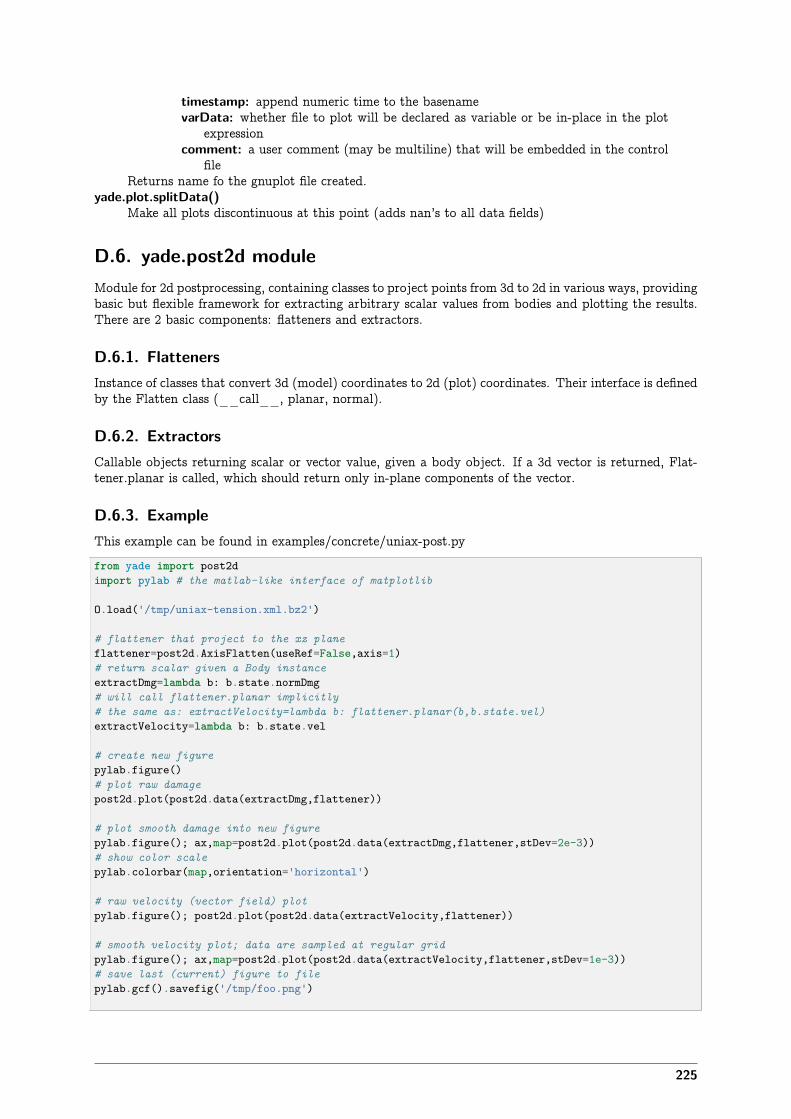
timestamp: append numeric time to the basenamevarData: whether file to plot will be declared as variable or be in-place in the plot

expressioncomment: a user comment (may be multiline) that will be embedded in the control

fileReturns name fo the gnuplot file created.

yade.plot.splitData()Make all plots discontinuous at this point (adds nan’s to all data fields)

D.6. yade.post2d moduleModule for 2d postprocessing, containing classes to project points from 3d to 2d in various ways, providingbasic but flexible framework for extracting arbitrary scalar values from bodies and plotting the results.There are 2 basic components: flatteners and extractors.

D.6.1. FlattenersInstance of classes that convert 3d (model) coordinates to 2d (plot) coordinates. Their interface is definedby the Flatten class (__call__, planar, normal).

D.6.2. ExtractorsCallable objects returning scalar or vector value, given a body object. If a 3d vector is returned, Flat-tener.planar is called, which should return only in-plane components of the vector.

D.6.3. ExampleThis example can be found in examples/concrete/uniax-post.pyfrom yade import post2dimport pylab # the matlab-like interface of matplotlib

O.load('/tmp/uniax-tension.xml.bz2')

# flattener that project to the xz planeflattener=post2d.AxisFlatten(useRef=False,axis=1)# return scalar given a Body instanceextractDmg=lambda b: b.state.normDmg# will call flattener.planar implicitly# the same as: extractVelocity=lambda b: flattener.planar(b,b.state.vel)extractVelocity=lambda b: b.state.vel

# create new figurepylab.figure()# plot raw damagepost2d.plot(post2d.data(extractDmg,flattener))

# plot smooth damage into new figurepylab.figure(); ax,map=post2d.plot(post2d.data(extractDmg,flattener,stDev=2e-3))# show color scalepylab.colorbar(map,orientation='horizontal')

# raw velocity (vector field) plotpylab.figure(); post2d.plot(post2d.data(extractVelocity,flattener))

# smooth velocity plot; data are sampled at regular gridpylab.figure(); ax,map=post2d.plot(post2d.data(extractVelocity,flattener,stDev=1e-3))# save last (current) figure to filepylab.gcf().savefig('/tmp/foo.png')

225

# show the figurespylab.show()

class yade.post2d.AxisFlatten(inherits Flatten)

__init__():parameters: ‘useRef‘: bool use reference positions rather than actual positions. ‘axis‘: {0,1,2}axis normal to the plane; the return value will be simply position with this component dropped.

normal()planar()

class yade.post2d.CylinderFlatten(inherits Flatten)Class for converting 3d point to 2d based on projection from circle. The y-axis in the projectioncorresponds to the rotation axis; the x-axis is distance form the axis.__init__()

:param useRef: (bool) use reference positions rather than actual positions :param axis: axisof the cylinder, �{0,1,2}

normal()planar()

class yade.post2d.FlattenAbstract class for converting 3d point into 2d. Used by post2d.data2d.normal()

Given position and vector value, return lenght of the vector normal to the flat plane.planar()

Given position and vector value, project the vector value to the flat plane and return its 2in-plane components.

class yade.post2d.SpiralFlatten(inherits Flatten)Class converting 3d point to 2d based on projection from spiral. The y-axis in the projectioncorresponds to the rotation axis__init__()

:parameters: ‘useRef‘: bool use reference positions rather than actual positions ‘thetaRange‘:(thetaMin,thetaMax) tuple bodies outside this range will be discarded ‘dH_dTheta‘:float in-clination of the spiral (per radian) ‘axis‘: {0,1,2} axis of rotation of the spiral ‘periodStart‘:float height of the spiral for zero angle

normal()planar()

yade.post2d.data(extractor, flattener, onlyDynamic=True, stDev=None, relThreshold=3.0,div=(50, 50), margin=(0, 0))

Filter all bodies (spheres only), project them to 2d and extract required scalar value; return eitherdiscrete array of positions and values, or smoothed data, depending on whether the stDev value isspecified.

Parametersextractor: callable receives Body instance, should return scalar, a 2-tuple (vector

fields) or None (to skip that body)flattener: callable receives Body instance and returns its 2d coordinates or None

(to skip that body)onlyDynamic: bool skip all non-dynamic bodiesstDev: float or None standard deviation for averaging, enables smoothing; None

(default) means raw mode.relThreshold: float threshold for the gaussian weight function relative to stDev

(smooth mode only)div: (int,int) number of cells for the gaussian grid (smooth mode only)margin: (float,float) margin around bounding box for data (smooth mode only)

Returns dictionaryReturned dictionary always containing keys ‘type’ (one of‘rawScalar’,’rawVector’,’smoothScalar’,’smoothVector’, depending on value of smooth and onreturn value from extractor), ‘x’, ‘y’, ‘bbox’.Raw data further contains ‘radii’.Scalar fields contain ‘val’ (value from extractor), vector fields have ‘valX’ and ‘valY’ (2 componentsreturned by the extractor).

226

yade.post2d.plot(data, axes=None, alpha=0.5, clabel=True, **kw)Given output from post2d.data, plot the scalar as discrete or smooth plot.For raw discrete data, plot filled circles with radii of particles, colored by the scalar value.For smooth discrete data, plot image with optional contours and contour labels.For vector data (raw or smooth), plot quiver (vector field), with arrows colored by the magnitude.

Parametersaxes: matplotlib.axes instance axes where the figure will be plotted; if None, will

be created from scratch.data: value returned by post2d.dataclable: bool show contour labels (smooth mode only)

Returns tuple of (axes,mappable); mappable can be used in further calls to py-lab.colorbar.

D.7. yade.qt moduleAccess/manipulation of the qt3-based yade gui.yade.qt.Controller() → None

Start simulation controlleryade.qt.Generator() → None

Start simulation generator (preprocessor interface)yade.qt.Renderer() → OpenGLRenderingEngine

Return wrapped OpenGLRenderingEngine; the renderer is constructed if it doesn’t exist yet.yade.qt.View() → GLViewer

Create new 3d view.yade.qt.activate() → None

Attempt to activate the Qt GUI.yade.qt.center() → None

Center all views.yade.qt.close() → None

Close all open qt windows.yade.qt.isActive() → bool

Whether the Qt GUI is being used.yade.qt.makePlayerVideo(*args, **kw)yade.qt.makeSimulationVideo(output, realPeriod=1, virtPeriod=0, iterPeriod=0, viewNo=0,

fps=24, msecSleep=0)Create video by running simulation. SnapshotEngine is added (and removed once done), temporaryfiles are deleted. The video is theora-encoded in the ogg container. Periodicity is controlled in thesame way as for PeriodicEngine (SnapshotEngine is a PeriodicEngine and realPeriod, virtPeriodand iterPeriod are passed to the new SnapshotEngine).viewNo is 0-based GL view number. 0 is the primary view and will be created if it doesn’t exist.It is an error if viewNo>0 and the view doesn’t exist.The simulation will run until it stops by itself. Either set Omega().stopAtIter or have an enginethat will call Omega().pause() at some point.See makePlayerVideo for more documentation.

yade.qt.views() → listReturn list of all open qt.GLViewer objects

yade._qt.Controller() → NoneStart simulation controller

class yade._qt.GLViewer

__init__() → None__init__((int)arg2) → None

axesShow arrows for axes.

center([(bool)median=True ]) → NoneCenter view. View is centered either so that all bodies fit inside (*median*=False), or so that75% of bodies fit inside (*median*=True).

eyePosition

227

Camera position.fitAABB((Vector3)mn, (Vector3)mx) → None

Adjust scene bounds so that Axis-aligned bounding box given by its lower and upper cornersmn, mx fits in.

fitSphere((Vector3)center, (float)radius) → NoneAdjust scene bounds so that sphere given by center and radius fits in.

fpsShow frames per second indicator.

gridDisplay square grid in zero planes, as 3-tuple of bools for yz, xz, xy planes.

loadState((int)slot) → NoneLoad display parameters from slot saved previously into, identified by its number.

lookAtPoint at which camera is directed.

orthoWhether orthographic projection is used; if false, use perspective projection.

saveState((int)slot) → NoneSave display parameters into numbered memory slot. Saves state for both GLViewer andassociated OpenGLRenderingEngine.

scaleScale of the view (?)

sceneRadiusVisible scene radius.

screenSizeSize of the viewer’s window, in scree pixels

showEntireScene() → NonetimeDisp

Time displayed on in the vindow; is a string composed of characters r, v, i standing respectivelyfor real time, virtual time, iteration number.

upVectorVector that will be shown oriented up on the screen.

viewDirCamera orientation (as vector).

yade._qt.Generator() → NoneStart simulation generator (preprocessor interface)

yade._qt.Renderer() → OpenGLRenderingEngineReturn wrapped OpenGLRenderingEngine; the renderer is constructed if it doesn’t exist yet.

yade._qt.View() → GLViewerCreate new 3d view.

yade._qt.activate() → NoneAttempt to activate the Qt GUI.

yade._qt.center() → NoneCenter all views.

yade._qt.close() → NoneClose all open qt windows.

yade._qt.isActive() → boolWhether the Qt GUI is being used.

yade._qt.views() → listReturn list of all open qt.GLViewer objects

D.8. yade.timing moduleFunctions for accessing timing information stored in engines and functors.

See Timing section of the programmer’s manual, wiki page for some examples.yade.timing.reset()

Zero all timing data.yade.timing.stats()

Print summary table of timing information from engines and functors. Absolute times as well as

228

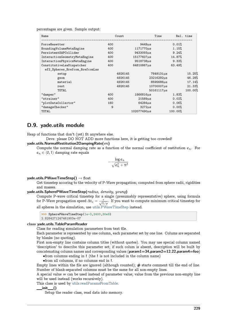
percentages are given. Sample output:Name Count Time Rel. time------------------------------------------------------------------------------------ForceResetter 400 9449µs 0.01%BoundingVolumeMetaEngine 400 1171770µs 1.15%PersistentSAPCollider 400 9433093µs 9.24%InteractionGeometryMetaEngine 400 15177607µs 14.87%InteractionPhysicsMetaEngine 400 9518738µs 9.33%ConstitutiveLawDispatcher 400 64810867µs 63.49%ef2_Spheres_Brefcom_BrefcomLaw

setup 4926145 7649131µs 15.25%geom 4926145 23216292µs 46.28%material 4926145 8595686µs 17.14%rest 4926145 10700007µs 21.33%TOTAL 50161117µs 100.00%

"damper" 400 1866816µs 1.83%"strainer" 400 21589µs 0.02%"plotDataCollector" 160 64284µs 0.06%"damageChecker" 9 3272µs 0.00%TOTAL 102077490µs 100.00%

D.9. yade.utils moduleHeap of functions that don’t (yet) fit anywhere else.

Devs: please DO NOT ADD more functions here, it is getting too crowded!yade.utils.NormalRestitution2DampingRate(en)

Compute the normal damping rate as a function of the normal coefficient of restitution en. Foren ∈ ⟨0, 1⟩ damping rate equals

−log en√e2n + π2

yade.utils.PWaveTimeStep() → floatGet timestep accoring to the velocity of P-Wave propagation; computed from sphere radii, rigiditiesand masses.

yade.utils.SpherePWaveTimeStep(radius, density, young)Compute P-wave critical timestep for a single (presumably representative) sphere, using formulafor P-Wave propagation speed ∆tc = r√

E/ρ. If you want to compute minimum critical timestep for

all spheres in the simulation, use utils.PWaveTimeStep instead.>>> SpherePWaveTimeStep(1e-3,2400,30e9)2.8284271247461903e-07

class yade.utils.TableParamReaderClass for reading simulation parameters from text file.Each parameter is represented by one column, each parameter set by one line. Colums are separatedby blanks (no quoting).First non-empty line contains column titles (without quotes). You may use special column named‘description’ to describe this parameter set; if such colum is absent, description will be built byconcatenating column names and corresponding values (param1=34,param2=12.22,param4=foo)

•from columns ending in ! (the ! is not included in the column name)•from all columns, if no columns end in !.

Empty lines within the file are ignored (although counted); # starts comment till the end of line.Number of blank-separated columns must be the same for all non-empty lines.A special value = can be used instead of parameter value; value from the previous non-empty linewill be used instead (works recursively).This class is used by utils.readParamsFromTable.__init__()

Setup the reader class, read data into memory.

229

paramDict()Return dictionary containing data from file given to constructor. Keys are line numbers (whichmight be non-contiguous and refer to real line numbers that one can see in text editors), valuesare dictionaries mapping parameter names to their values given in the file. The special value‘=’ has already been interpreted, ! (bangs) (if any) were already removed from column titles,description column has already been added (if absent).

yade.utils.aabbDim(cutoff=0.0, centers=False)Return dimensions of the axis-aligned bounding box, optionally with relative part cutoff cut away.

yade.utils.aabbExtrema([(float)cutoff=0.0[, (bool)centers=False ] ]) → tupleReturn coordinates of box enclosing all bodies

Parameters• centers (bool) – do not take sphere radii in account, only their centroids• cutoff (float�⟨0…1⟩) – relative dimension by which the box will be cut away

at its boundaries.Returns (lower corner, upper corner) as (Vector3,Vector3)

yade.utils.aabbExtrema2d(pts)Return 2d bounding box for a sequence of 2-tuples.

yade.utils.aabbWalls(extrema=None, thickness=None, oversizeFactor=1.5, **kw)Return 6 boxes that will wrap existing packing as walls from all sides; extrema are extremal points ofthe Aabb of the packing (will be calculated if not specified) thickness is wall thickness (will be 1/10of the X-dimension if not specified) Walls will be enlarged in their plane by oversizeFactor. returnslist of 6 wall Bodies enclosing the packing, in the order minX,maxX,minY,maxY,minZ,maxZ.

yade.utils.approxSectionArea((float)arg1, (int)arg2) → floatCompute area of convex hull when when taking (swept) spheres crossing the plane at coord, per-pendicular to axis.

yade.utils.avgNumInteractions(cutoff=0.0)Return average numer of interactions per particle, also known as coordination number.

Parameters• cutoff – cut some relative part of the sample’s bounding box away.

yade.utils.bodyNumInteractionsHistogram([(tuple)aabb ]) → tupleyade.utils.box(center, extents, orientation=[, 1, 0, 0, 0 ], dynamic=True, wire=False,

color=None, highlight=False, material=-1, mask=1)Create box (cuboid) with given parameters.

Parametersextents: Vector3 half-sizes along x,y,z axes

See utils.sphere‘s documentation for meaning of other parameters.yade.utils.coordsAndDisplacements((int)axis[, (tuple)Aabb=() ]) → tuple

Return tuple of 2 same-length lists for coordinates and displacements (coordinate minus referencecoordinate) along given axis (1st arg); if the Aabb=((x_min,y_min,z_min),(x_max,y_max,z_-max)) box is given, only bodies within this box will be considered.

yade.utils.createInteraction((int)id1, (int)id2) → InteractionCreate interaction between given bodies by hand.Current engines are searched for InteractionGeometryDispatcher and InteractionPhysicsDispatcher(might be both hidden in InteractionDispatchers). Geometry is created using force parameter ofthe geometry dispatcher, wherefore the interaction will exist even if bodies do not spatially overlapand the functor would return false under normal circumstances.This function will very likely behave incorrectly for periodic simulations (though it could be ex-tended it to handle it farily easily).

yade.utils.defaultMaterial()Return default material, when creating bodies with utils.sphere and friends, material is unspecifiedand there is no shared material defined yet. By default, this function returns:FrictMat(density=1e3,young=1e7,poisson=.3,frictionAngle=.5,label=’defaultMat’)

yade.utils.downCast(obj, newClassName)Cast given object to class deriving from the same yade root class and copy all parameters from givenobject. Obj should be up in the inheritance tree, otherwise some attributes may not be defined inthe new class.

yade.utils.elasticEnergy((tuple)arg1) → floatyade.utils.encodeVideoFromFrames(frameSpec, out, renameNotOverwrite=True, fps=24)

230

Create .ogg video from external image files.Parameters

frameSpec: wildcard | sequence of filenames If string, wildcard in format under-stood by GStreamer’s multifilesrc plugin (e.g. ‘/tmp/frame-%04d.png’). If listor tuple, filenames to be encoded in given order.

Warning: GStreamer is picky about the wildcard; if you pass a wrong one,if will not complain, but silently stall.

out: filename file to save video intorenameNotOverwrite: bool if True, existing same-named video file will have ~[num-

ber] appended; will be overwritten otherwise.fps: Frames per second.

yade.utils.facet(vertices, dynamic=False, wire=True, color=None, highlight=False,noBound=False, material=-1, mask=1)

Create facet with given parameters.Parameters

vertices: [Vector3,Vector3,Vector3] coordinates of vertices in the global coordinatesystem.

wire: bool if True, facets are shown as skeleton; otherwise facets are fillednoBound: do not assign Body().boundcolor: Vector3 or None random color will be assigned if Nonematerial: int | string | Material instance | callable returning Material instance

• if int, O.materials[material] will be used; as a special case, if material==-1 andthere is no shared materials defined, utils.defaultMaterial() will be assigned toO.materials[0]

• if string, it is label of an existing material that will be used• if Material instance, this instance will be used• if callable, it will be called without arguments; returned Material value will be

used (Material factory object, if you like)mask: integer Body.mask for the body

See utils.sphere‘s documentation for meaning of other parameters.yade.utils.facetBox(center, extents, orientation=Quaternion((1, 0, 0), 0), wallMask=63,

**kw)Create arbitrarily-aligned box composed of facets, with given center, extents and orientation. Ifany of the box dimensions is zero, corresponding facets will not be created. The facets are orientedoutwards from the box.

Parameterscenter: Vector3 center of the created boxextents: (eX,eY,eZ) lengths of the box sidesorientation: quaternion orientation of the boxwallMask: bitmask determines which walls will be created, in the order -x (1), +x

(2), -y (4), +y (8), -z (16), +z (32). The numbers are ANDed; the default 63means to create all walls;

**kw: (unused keyword arguments) passed to utils.facetReturns list of facets forming the box.

yade.utils.facetCylinder(center, radius, height, orientation=[, 1, 0, 0, 0 ], segmentsNumber=10,wallMask=7, closed=1, **kw)

Create arbitrarily-aligned cylinder composed of facets, with given center, radius, height and orien-tation. Return List of facets forming the cylinder;

Parameterscenter: Vector3 center of the created cylinderradius: float cylinder radiusheight: float cylinder heightorientation: Quaternion orientation of the cylindersegmentsNumber: int number of edges on the cylinder surface (>=5)wallMask: bitmask determines which walls will be created, in the order up (1), down

(2), side (4). The numbers are ANDed; the default 7 means to create all walls;**kw: (unused keyword arguments) passed to utils.facet;

231

yade.utils.flipCell([(Matrix3)flip=Matrix3(0, 0, 0, 0, 0, 0, 0, 0, 0) ]) → Matrix3Flip periodic cell so that angles between R3 axes and transformed axes are as small as possible.This function relies on the fact that periodic cell defines by repetition or its corners regular grid ofpoints in R3; however, all cells generating identical grid are equivalent and can be flipped one overanother. This necessiatates adjustment of Interaction.cellDist for interactions that cross boundaryand didn’t before (or vice versa), and re-initialization of collider. The flip argument can be usedto specify desired flip: integers, each column for one axis; if zero matrix, best fit (minimizing theangles) is computed automatically.In c++, this function is accessible as Shop::flipCell.This function is currently broken and should not be used.

yade.utils.forcesOnCoordPlane((float)arg1, (int)arg2) → Vector3yade.utils.forcesOnPlane((Vector3)planePt, (Vector3)normal) → Vector3

Find all interactions deriving from NormShearPhys that cross given plane and sum forces (bothnormal and shear) on them.

Parameters• planePt (Vector3) – a point on the plane• normal (Vector3) – plane normal (will be normalized).

yade.utils.fractionalBox(fraction=1.0, minMax=None)retrurn (min,max) that is the original minMax box (or aabb of the whole simulation if not specified)linearly scaled around its center to the fraction factor

yade.utils.getSpheresVolume() → floatCompute the total volume of spheres in the simulation (might crash for now if dynamic bodies arenot spheres)

yade.utils.getViscoelasticFromSpheresInteraction((float)m, (float)tc, (float)en, (float)es) →dict

Get viscoelastic interaction parameters from analytical solution of a pair spheres collision problem.Parameters

‘m‘ : float sphere mass ‘tc‘ : float collision time ‘en‘ : float normal restitution coefficient ‘es‘ : floattangential restitution coefficient.

Returnsdict with keys:kn : float normal elastic coefficient computed as:

kn =m

t2c

(π2 + (ln en)2

)

cn : float normal viscous coefficient computed as:

cn = −2m

tcln en

kt : float tangential elastic coefficient computed as:

kt =2

7

m

t2c

(π2 + (ln et)2

)

ct : float tangential viscous coefficient computed as:

ct = −2

7

m

tcln et.

For details see [48].yade.utils.highlightNone() → None

Reset highlight on all bodies.yade.utils.inscribedCircleCenter((Vector3)v1, (Vector3)v2, (Vector3)v3) → Vector3

Return center of inscribed circle for triangle given by its vertices v1, v2, v3.

232

yade.utils.interactionAnglesHistogram((int)axis[, (int)mask[, (int)bins[, (tuple)aabb ] ] ]) →tuple

yade.utils.kineticEnergy() → floatCompute overall kinetic energy of the simulation as∑ 1

2

(miv

2i +ω(IωT )

).

No transformation of inertia tensor (in local frame) I is done, although it is multiplied by angularvelocity ω (in global frame); the value will not be accurate for aspherical particles.

yade.utils.loadVars(mark=None)Load variables from saveVars, which are saved inside the simulation. If mark==None, all savevariables are loaded. Otherwise only those with the mark passed.

yade.utils.negPosExtremeIds((int)axis[, (float)distFactor ]) → tupleReturn list of ids for spheres (only) that are on extremal ends of the specimen along given axis;distFactor multiplies their radius so that sphere that do not touch the boundary coordinate canalso be returned.

yade.utils.perpendicularArea(axis)Return area perpendicular to given axis (0=x,1=y,2=z) generated by bodies for which the functionconsider returns True (defaults to returning True always) and which is of the type Sphere.

yade.utils.plotDirections(aabb=(), mask=0, bins=20, numHist=True)Plot 3 histograms for distribution of interaction directions, in yz,xz and xy planes and (optionalbut default) histogram of number of interactions per body.

yade.utils.plotNumInteractionsHistogram(cutoff=0.0)Plot histogram with number of interactions per body, optionally cutting away cutoff relative axis-aligned box from specimen margin.

yade.utils.pointInsidePolygon((tuple)arg1, (object)arg2) → boolyade.utils.ptInAABB((tuple)arg1, (tuple)arg2, (tuple)arg3) → bool

Return True/False whether the point (3-tuple) p is within box given by its min (3-tuple) and max(3-tuple) corners

yade.utils.randomColor()Return random Vector3 with each component in interval 0…1 (uniform distribution)

yade.utils.randomizeColors(onlyDynamic=False)Assign random colors to Shape::color.If onlyDynamic is true, only dynamic bodies will have the color changed.

yade.utils.readParamsFromTable(tableFileLine=None, noTableOk=False, unknownOk=False,**kw)

Read parameters from a file and assign them to __builtin__ variables.The format of the file is as follows (commens starting with # and empty lines allowed):

# commented lines allowed anywherename1 name2 … # first non-blank line are column headings

# empty line is OK, with or without commentval1 val2 … # 1st parameter setval2 val2 … # 2nd…

Assigned tags:•description column is assigned to Omega().tags[’description’]; this column is synthesized ifabsent (see utils.TableParamReader)

•Omega().tags[’params’]=”name1=val1,name2=val2,…”•Omega().tags[’defaultParams’]=”unassignedName1=defaultValue1,…”

All parameters (default as well as settable) are saved using saveVars(‘table’).Parameters

tableFile: text file (with one value per blank-separated columns)tableLine: number of line where to get the values from.noTableOk: bool do not raise exception if the file cannot be open; use default valuesunknownOk: bool do not raise exception if unknown column name is found in the

file; assign it as wellReturns number of assigned parameters.

233

yade.utils.replaceCollider(colliderEngine)Replaces collider (Collider) engine with the engine supplied. Raises error if no collider is in engines.

yade.utils.saveVars(mark=’‘, loadNow=False, **kw)Save passed variables into the simulation so that it can be recovered when the simulation is loadedagain.For example, variables a=5, b=66 and c=7.5e-4 are defined. To save those, use:

>>> from yade import utils>>> utils.saveVars('mark',a=1,b=2,c=3,loadNow=True)>>> a,b,c(1, 2, 3)

those variables will be save in the .xml file, when the simulation itself is saved. To recover thosevariables once the .xml is loaded again, use

>>> utils.loadVars('mark')

and they will be defined in the __builtin__ namespace (i.e. available from anywhere in the pythoncode).If loadParam*==True, variables will be loaded immediately after saving. That effectivelymakes ***kw available in builtin namespace.

yade.utils.scalarOnColorScale((float)arg1, (float)arg2, (float)arg3) → Vector3yade.utils.setRefSe3() → None

Set reference positions and orientations of all bodies equal to their current positions and orienta-tions.

yade.utils.sphere(center, radius, dynamic=True, wire=False, color=None, highlight=False,material=-1, mask=1)

Create sphere with given parameters; mass and inertia computed automatically.Last assigned material is used by default (*material*=-1), and utils.defaultMaterial() will be usedif no material is defined at all.

Parameterscenter: Vector3 centerradius: float radiuscolor: Vector3 or None random color will be assigned if Nonematerial: int | string | Material instance | callable returning Material instance

• if int, O.materials[material] will be used; as a special case, if material==-1 andthere is no shared materials defined, utils.defaultMaterial() will be assigned toO.materials[0]

• if string, it is label of an existing material that will be used• if Material instance, this instance will be used• if callable, it will be called without arguments; returned Material value will be

used (Material factory object, if you like)mask: integer Body.mask for the body

Returns A Body instance with desired characteristics.Creating default shared material if none exists neither is given:

>>> O.reset()>>> from yade import utils>>> len(O.materials)0>>> s0=utils.sphere([2,0,0],1)>>> len(O.materials)1

Instance of material can be given:

>>> s1=utils.sphere([0,0,0],1,wire=False,color=(0,1,0),material=ElastMat(young=30e9,density=2e3))>>> s1.shape.wireFalse>>> s1.shape.colorVector3(0,1,0)>>> s1.mat.density2000.0

234

Material can be given by label:

>>> O.materials.append(FrictMat(young=10e9,poisson=.11,label='myMaterial'))1>>> s2=utils.sphere([0,0,2],1,material='myMaterial')>>> s2.mat.label'myMaterial'>>> s2.mat.poisson0.11

Finally, material can be a callable object (taking no arguments), which returns a Material instance.Use this if you don’t call this function directly (for instance, through yade.pack.randomDensePack),passing only 1 material parameter, but you don’t want material to be shared.For instance, randomized material properties can be created like this:

>>> import random>>> def matFactory(): return ElastMat(young=1e10*random.random(),density=1e3+1e3*random.random())...>>> s3=utils.sphere([0,2,0],1,material=matFactory)>>> s4=utils.sphere([1,2,0],1,material=matFactory)

yade.utils.spiralProject((Vector3)pt, (float)dH_dTheta[, (int)axis=2[,(float)periodStart=nan[, (float)theta0=0 ] ] ]) → tuple

yade.utils.sumFacetNormalForces((object)ids[, (int)axis=-1 ]) → floatSum force magnitudes on given bodies (must have shape of the Facet type), considering only partof forces perpendicular to each facet’s face; if axis has positive value, then the specified axis (0=x,1=y, 2=z) will be used instead of facet’s normals.

yade.utils.sumForces((tuple)ids, (Vector3)direction) → floatReturn summary force on bodies with given ids, projected on the direction vector.

yade.utils.sumTorques((tuple)ids, (Vector3)axis, (Vector3)axisPt) → floatSum forces and torques on bodies given in ids with respect to axis specified by a point axisPt andits direction axis.

yade.utils.totalForceInVolume() → tupleReturn summed forces on all interactions and average isotropic stiffness, as tuple (Vector3,float)

yade.utils.typedEngine(name)Return first engine from current O.engines, identified by its type (as string). For example:

>>> from yade import utils>>> O.engines=[InsertionSortCollider(),NewtonIntegrator(),GravityEngine()]>>> utils.typedEngine("NewtonIntegrator") == O.engines[1]True

yade.utils.unbalancedForce([(bool)useMaxForce=False ]) → floatCompute the ratio of mean (or maximum, if useMaxForce) summary force on bodies and maximumforce magnitude on interactions. For perfectly static equilibrium, summary force on all bodies is zero(since forces from interactions cancel out and induce no acceleration of particles); this ratio will tendto zero as simulation stabilizes, though zero is never reached because of finite precision computation.Sufficiently small value can be e.g. 1e-2 or smaller, depending on how much equilibrium it shouldbe.

yade.utils.uniaxialTestFeatures(filename=None, areaSections=10, axis=-1, **kw)Get some data about the current packing useful for uniaxial test:

1.Find the dimensions that is the longest (uniaxial loading axis)2.Find the minimum cross-section area of the specimen by examining several (areaSections)sections perpendicular to axis, computing area of the convex hull for each one. This will workalso for non-prismatic specimen.

3.Find the bodies that are on the negative/positive boundary, to which the straining conditionshould be applied.Parameters

filename: if given, spheres will be loaded from this file (ASCII format); if not, currentsimulation will be used.

areaSection: number of section that will be used to estimate cross-sectionaxis: if given, force strained axis, rather than computing it from predominant length

235

Returns dictionary with keys ‘negIds’, ‘posIds’, ‘axis’, ‘area’.Warning: The function utils.approxSectionArea uses convex hull algorithm to find the area,but the implementation is reported to be buggy (bot works in some cases). Always check thisnumber, or fix the convex hull algorithm (it is documented in the source, see py/_utils.cpp).

yade.utils.vmData()Return memory usage data from Linux’s /proc/[pid]/status, line VmData.

yade.utils.wall(position, axis, sense=0, color=None, material=-1, mask=1)Return ready-made wall body.

Parametersposition: float or Vector3 center of the wall. If float, it is the position along given

axis, the other 2 components being zeroaxis: �{0,1,2} orientation of the wall normal (0,1,2) for x,y,z (sc. planes yz, xz, xy)sense: �{-1,0,1} sense in which to interact (0: both, -1: negative, +1: positive; see

Wall reference documentation)mask: bitmask (as int) Body.mask

See utils.sphere‘s documentation for meaning of other parameters.yade.utils.wireAll() → None

Set Shape::wire on all bodies to True, rendering them with wireframe only.yade.utils.wireNoSpheres() → None

Set Shape::wire to True on non-spherical bodies (Facets, Walls).yade.utils.wireNone() → None

Set Shape::wire on all bodies to False, rendering them as solids.yade.utils.xMirror(half )

Mirror a sequence of 2d points around the x axis (changing sign on the y coord). The sequenceshould start up and then it will wrap from y downwards (or vice versa). If the last point’s x coordis zero, it will not be duplicated.

yade._utils.PWaveTimeStep() → floatGet timestep accoring to the velocity of P-Wave propagation; computed from sphere radii, rigiditiesand masses.

yade._utils.aabbExtrema([(float)cutoff=0.0[, (bool)centers=False ] ]) → tupleReturn coordinates of box enclosing all bodies

Parameters• centers (bool) – do not take sphere radii in account, only their centroids• cutoff (float�⟨0…1⟩) – relative dimension by which the box will be cut away

at its boundaries.Returns (lower corner, upper corner) as (Vector3,Vector3)

yade._utils.approxSectionArea((float)arg1, (int)arg2) → floatCompute area of convex hull when when taking (swept) spheres crossing the plane at coord, per-pendicular to axis.

yade._utils.bodyNumInteractionsHistogram([(tuple)aabb ]) → tupleyade._utils.coordsAndDisplacements((int)axis[, (tuple)Aabb=() ]) → tuple

Return tuple of 2 same-length lists for coordinates and displacements (coordinate minus referencecoordinate) along given axis (1st arg); if the Aabb=((x_min,y_min,z_min),(x_max,y_max,z_-max)) box is given, only bodies within this box will be considered.

yade._utils.createInteraction((int)id1, (int)id2) → InteractionCreate interaction between given bodies by hand.Current engines are searched for InteractionGeometryDispatcher and InteractionPhysicsDispatcher(might be both hidden in InteractionDispatchers). Geometry is created using force parameter ofthe geometry dispatcher, wherefore the interaction will exist even if bodies do not spatially overlapand the functor would return false under normal circumstances.This function will very likely behave incorrectly for periodic simulations (though it could be ex-tended it to handle it farily easily).

yade._utils.elasticEnergy((tuple)arg1) → floatyade._utils.flipCell([(Matrix3)flip=Matrix3(0, 0, 0, 0, 0, 0, 0, 0, 0) ]) → Matrix3

Flip periodic cell so that angles between R3 axes and transformed axes are as small as possible.This function relies on the fact that periodic cell defines by repetition or its corners regular grid of

236

points in R3; however, all cells generating identical grid are equivalent and can be flipped one overanother. This necessiatates adjustment of Interaction.cellDist for interactions that cross boundaryand didn’t before (or vice versa), and re-initialization of collider. The flip argument can be usedto specify desired flip: integers, each column for one axis; if zero matrix, best fit (minimizing theangles) is computed automatically.In c++, this function is accessible as Shop::flipCell.This function is currently broken and should not be used.

yade._utils.forcesOnCoordPlane((float)arg1, (int)arg2) → Vector3yade._utils.forcesOnPlane((Vector3)planePt, (Vector3)normal) → Vector3

Find all interactions deriving from NormShearPhys that cross given plane and sum forces (bothnormal and shear) on them.

Parameters• planePt (Vector3) – a point on the plane• normal (Vector3) – plane normal (will be normalized).

yade._utils.getSpheresVolume() → floatCompute the total volume of spheres in the simulation (might crash for now if dynamic bodies arenot spheres)

yade._utils.getViscoelasticFromSpheresInteraction((float)m, (float)tc, (float)en, (float)es) →dict

Get viscoelastic interaction parameters from analytical solution of a pair spheres collision problem.Parameters

‘m‘ : float sphere mass ‘tc‘ : float collision time ‘en‘ : float normal restitution coefficient ‘es‘ : floattangential restitution coefficient.

Returnsdict with keys:kn : float normal elastic coefficient computed as:

kn =m

t2c

(π2 + (ln en)2

)

cn : float normal viscous coefficient computed as:

cn = −2m

tcln en

kt : float tangential elastic coefficient computed as:

kt =2

7

m

t2c

(π2 + (ln et)2

)

ct : float tangential viscous coefficient computed as:

ct = −2

7

m

tcln et.

For details see [48].yade._utils.highlightNone() → None

Reset highlight on all bodies.yade._utils.inscribedCircleCenter((Vector3)v1, (Vector3)v2, (Vector3)v3) → Vector3

Return center of inscribed circle for triangle given by its vertices v1, v2, v3.yade._utils.interactionAnglesHistogram((int)axis[, (int)mask[, (int)bins[, (tuple)aabb ] ] ]) →

tupleyade._utils.kineticEnergy() → float

Compute overall kinetic energy of the simulation as∑ 1

2

(miv

2i +ω(IωT )

).

237

No transformation of inertia tensor (in local frame) I is done, although it is multiplied by angularvelocity ω (in global frame); the value will not be accurate for aspherical particles.

yade._utils.negPosExtremeIds((int)axis[, (float)distFactor ]) → tupleReturn list of ids for spheres (only) that are on extremal ends of the specimen along given axis;distFactor multiplies their radius so that sphere that do not touch the boundary coordinate canalso be returned.

yade._utils.pointInsidePolygon((tuple)arg1, (object)arg2) → boolyade._utils.ptInAABB((tuple)arg1, (tuple)arg2, (tuple)arg3) → bool

Return True/False whether the point (3-tuple) p is within box given by its min (3-tuple) and max(3-tuple) corners

yade._utils.scalarOnColorScale((float)arg1, (float)arg2, (float)arg3) → Vector3yade._utils.setRefSe3() → None

Set reference positions and orientations of all bodies equal to their current positions and orienta-tions.

yade._utils.spiralProject((Vector3)pt, (float)dH_dTheta[, (int)axis=2[,(float)periodStart=nan[, (float)theta0=0 ] ] ]) → tuple

yade._utils.sumFacetNormalForces((object)ids[, (int)axis=-1 ]) → floatSum force magnitudes on given bodies (must have shape of the Facet type), considering only partof forces perpendicular to each facet’s face; if axis has positive value, then the specified axis (0=x,1=y, 2=z) will be used instead of facet’s normals.

yade._utils.sumForces((tuple)ids, (Vector3)direction) → floatReturn summary force on bodies with given ids, projected on the direction vector.

yade._utils.sumTorques((tuple)ids, (Vector3)axis, (Vector3)axisPt) → floatSum forces and torques on bodies given in ids with respect to axis specified by a point axisPt andits direction axis.

yade._utils.totalForceInVolume() → tupleReturn summed forces on all interactions and average isotropic stiffness, as tuple (Vector3,float)

yade._utils.unbalancedForce([(bool)useMaxForce=False ]) → floatCompute the ratio of mean (or maximum, if useMaxForce) summary force on bodies and maximumforce magnitude on interactions. For perfectly static equilibrium, summary force on all bodies is zero(since forces from interactions cancel out and induce no acceleration of particles); this ratio will tendto zero as simulation stabilizes, though zero is never reached because of finite precision computation.Sufficiently small value can be e.g. 1e-2 or smaller, depending on how much equilibrium it shouldbe.

yade._utils.wireAll() → NoneSet Shape::wire on all bodies to True, rendering them with wireframe only.

yade._utils.wireNoSpheres() → NoneSet Shape::wire to True on non-spherical bodies (Facets, Walls).

yade._utils.wireNone() → NoneSet Shape::wire on all bodies to False, rendering them as solids.

D.10. yade.ymport moduleImport geometry from various formats (‘import’ is python keyword, hence the name ‘ymport’).yade.ymport.gengeo(mntable, shift=Vector3(0, 0, 0), scale=1.0, **kw)

Imports geometry from LSMGenGeo library and creates spheres.Parameters

mntable: mntable object, which creates by LSMGenGeo library, see exampleshift: [float,float,float] [X,Y,Z] parameter moves the specimen.scale: float factor scales the given data.**kw: (unused keyword arguments) is passed to utils.sphere

LSMGenGeo library allows to create pack of spheres with given [Rmin:Rmax] with null stress insidethe specimen. Can be useful for Mining Rock simulation.Example: examples/regular-sphere-pack/regular-sphere-pack.py, usage of LSMGenGeo library inscripts/test/genCylLSM.py.

•https://answers.launchpad.net/esys-particle/+faq/877•http://www.access.edu.au/lsmgengeo_python_doc/current/pythonapi/html/GenGeo-

238

module.html•https://svn.esscc.uq.edu.au/svn/esys3/lsm/contrib/LSMGenGeo/

yade.ymport.gengeoFile(fileName=’file.geo’, shift=[, 0.0, 0.0, 0.0 ], scale=1.0, **kw)Imports geometry from LSMGenGeo .geo file and creates spheres.

Parametersfilename: string file which has 4 colums [x, y, z, radius].shift: [float,float,float] [X,Y,Z] parameter moves the specimen.scale: float factor scales the given data.**kw: (unused keyword arguments) is passed to utils.sphere

Returns list of spheres.LSMGenGeo library allows to create pack of spheres with given [Rmin:Rmax] with null stress insidethe specimen. Can be useful for Mining Rock simulation.Example: examples/regular-sphere-pack/regular-sphere-pack.py, usage of LSMGenGeo library inscripts/test/genCylLSM.py.

•https://answers.launchpad.net/esys-particle/+faq/877•http://www.access.edu.au/lsmgengeo_python_doc/current/pythonapi/html/GenGeo-module.html

•https://svn.esscc.uq.edu.au/svn/esys3/lsm/contrib/LSMGenGeo/yade.ymport.gmsh(meshfile=’file.mesh’, shift=[, 0.0, 0.0, 0.0 ], scale=1.0, orienta-

tion=Quaternion((1, 0, 0), 0), **kw)Imports geometry from mesh file and creates facets.

Parametersshift: [float,float,float] [X,Y,Z] parameter moves the specimen.scale: float factor scales the given data.orientation: quaternion orientation of the imported mesh**kw: (unused keyword arguments) is passed to utils.facet

Returns list of facets forming the specimen.mesh files can be easily created with GMSH. Example added to examples/regular-sphere-pack/regular-sphere-pack.pyAdditional examples of mesh-files can be downloaded from http://www-roc.inria.fr/gamma/download/download.php

yade.ymport.gts(meshfile, shift=(0, 0, 0), scale=1.0, **kw)Read given meshfile in gts format.

Parametersmeshfile: string name of the input file.shift: [float,float,float] [X,Y,Z] parameter moves the specimen.scale: float factor scales the given data.**kw: (unused keyword arguments) is passed to utils.facet

Returns list of facets.yade.ymport.stl(file, dynamic=False, wire=True, color=None, highlight=False,

noBound=False, material=-1)Import geometry from stl file, return list of created facets.

yade.ymport.text(fileName, shift=[, 0.0, 0.0, 0.0 ], scale=1.0, **kw)Load sphere coordinates from file, create spheres, insert them to the simulation.

Parametersfilename: string file which has 4 colums [x, y, z, radius].shift: [float,float,float] [X,Y,Z] parameter moves the specimen.scale: float factor scales the given data.**kw: (unused keyword arguments) is passed to utils.sphere

Returns list of spheres.Lines starting with # are skipped

yade.ymport.textExt(fileName, format=’x_y_z_r’, shift=[, 0.0, 0.0, 0.0 ], scale=1.0, **kw)Load sphere coordinates from file in specific format, create spheres, insert them to the simulation.

Parameters filename: string format:the name of output format. Supported x_y_z_r‘(default), ‘x_y_z_r_-matId

shift: [float,float,float] [X,Y,Z] parameter moves the specimen.scale: float factor scales the given data.

239

**kw: (unused keyword arguments) is passed to utils.sphereReturns list of spheres.

Lines starting with # are skipped

240

Bibliography

[1] M. P. Allen and D. J. Tildesley. Computer simulation of liquids. Clarendon Press, New York, NY,USA, 1989. ISBN 0-19-855645-4.

[2] F. Alonso-Marroquín, R. García-Rojo, and H. J. Herrmann. Micro-mechanical investigation of thegranular ratcheting. In T. Triantafyllidis, editor, Cyclic Behaviour of Soils and LiquefactionPhenomena, pages 3–10. Taylor & Francis, april 2004. ISBN 9058096203. URL http://www.comphys.ethz.ch/hans/p/334.pdf.

[3] Peter F. Ash and Ethan D. Bolker. Generalized dirichlet tessellations. Geometriae Dedicata, 20(2):209–243, April 1986. ISSN 0046-5755 (Print) 1572-9168 (Online). doi: 10.1007/BF00164401. URLhttp://www.springerlink.com/content/j334537p07370405/.

[4] N. Bićanić. Discrete Element Methods. In E. Stein, R. de Borst, and T.J.R. Hughes, editors,Encyclopedia of Computational Mechanics: Fundametals, pages 311–337. Wiley and Sons, 2004.

[5] F. Camborde, C. Mariotti, and F. V. Donzé. Numerical study of rock and concrete behaviourby discrete element modelling. Computers and Geotechnics, 27(4):225–247, 2000. URL http://dx.doi.org/10.1016/S0266-352X(00)00013-6.

[6] Ferhun C. Caner and Zdenek P. Bažant. Microplane model m4 for concrete. ii: Algorithm andcalibration. Journal of Engineering Mechanics, 126(9):954–961, 2000. doi: 10.1061/(ASCE)0733-9399(2000)126:9(954). URL http://www.civil.northwestern.edu/people/bazant/PDFs/Papers/394.pdf.

[7] Bruno Chareyre and Pascal Villard. Dynamic spar elements and discrete element methods in twodimensions for the modeling of soil-inclusion problems. Journal of Engineering Mechanics, 131(7):689–698, 2005. doi: 10.1061/(ASCE)0733-9399(2005)131:7(689). URL http://link.aip.org/link/?QEM/131/689/1.

[8] P. A. Cundall and O. D. L. Strack. A discrete numerical model for granular assemblies. Geotech-nique, 29(1):47–65, 1979.

[9] Gianluca Cusatis, Zdenek P. Bažant, and Luigi Cedolin. Confinement-shear lattice model for con-crete damage in tension and compression: I. theory. Journal of Engineering Mechanics, 129(12):1439–1448, 2003. URL http://scitation.aip.org/getabs/servlet/GetabsServlet?prog=normal&id=JENMDT000129000012001439000001&idtype=cvips&gifs=yes.

[10] G. A. D’Addetta, F. Kun, E. Ramm, and H. J. Herrmann. From solids to granulates - Discreteelement simulations of fracture and fragmentation processes in geomaterials. In P. A. Vermeer,S. Diebels, W. Ehlers, H. J. Herrmann, S. Luding, & E. Ramm, editor, Continuous and Discontin-uous Modelling of Cohesive-Frictional Materials, volume 568 of Lecture Notes in Physics, BerlinSpringer Verlag, pages 231–+, 2001. URL http://www.comphys.ethz.ch/hans/p/267.pdf.

[11] F. V. Donzé. Spherical discrete element code, 1997. URL http://geo.hmg.inpg.fr/frederic/articles/sdec_v2.00.pdf.

[12] Ulrich Drepper. What Every Programmer Should Know About Memory. 2007. URL http://people.redhat.com/drepper/cpumemory.pdf.

[13] Karel Driesen and Urs Hölzle. The direct cost of virtual function calls in c++. In OOPSLA ’96:Proceedings of the 11th ACM SIGPLAN conference on Object-oriented programming, systems,languages, and applications, pages 306–323, New York, NY, USA, 1996. ACM. ISBN 0-89791-788-X. doi: http://doi.acm.org/10.1145/236337.236369.

[14] ESyS-Particle. Esys-particle, February 2010. URL https://launchpad.net/esys-particle/.

241

[15] Euler angles. Euler angles, February 2010. URL http://en.wikipedia.org/wiki/Euler_angles.[16] Peter Grassl and Milan Jirásek. Damage-plastic model for concrete failure. International Jour-

nal of Solids and Structures, 43(22-23):7166–7196, 2006. ISSN 0020-7683. doi: DOI:10.1016/j.ijsolstr.2006.06.032. URL http://www.sciencedirect.com/science/article/B6VJS-4K8NWXK-1/2/e3a41b693b156ce13a70e44e973d505f.

[17] D. V. Griffiths and G. G. W. Mustoe. Modelling of elastic continua using a grillage of structuralelements based on discrete element concepts. International Journal for Numerical Methods inEngineering, 50(7):1759–1775, 2001. doi: 10.1002/nme.99. URL http://80.www3.interscience.wiley.com.dialog.cvut.cz/journal/76509666/abstract.

[18] Sir William Rowan Hamilton. Lectures on quaternions, 1853. URL http://books.google.com/books?id=TCwPAAAAIAAJ.

[19] Sébastien Hentz. Modélisation d’une Structure en Béton Armé Soumise à un Choc par laméthode des Éléments Discrets. PhD thesis, Université Grenoble 1 – Joseph Fourier, October2003.

[20] Sébastien Hentz, Laurent Daudeville, and Frédéric V. Donzé. Identification and validation of adiscrete element model for concrete. Journal of Engineering Mechanics, 130(6):709–719, June2004.

[21] Alexander Hrennikoff. Solution of problems of elasticity by the frame-work method. ASME Journalof Applied Mechanics, (8):A619–A715, 1941.

[22] Philip M. Hubbard. Approximating polyhedra with spheres for time-critical collision detection.ACM Trans. Graph., 15(3):179–210, 1996. ISSN 0730-0301. doi: http://doi.acm.org/10.1145/231731.231732.

[23] ICG. PFC3D (Particle Flow Code in 3D) Theory and Background Manual, version 3.0. ItascaConsulting Group, 2003.

[24] Jean-François Jerier, Didier Imbault, Fréderic-Victor Donzé, and Pierre Doremus. A geometricalgorithm based on tetrahedral meshes to generate a dense polydisperse sphere packing. GranularMatter, 11(1):43–52, 2009. doi: 10.1007/s10035-008-0116-0. URL http://www.springerlink.com/content/w0x307g110421035.

[25] Scott M. Johnson, John R. Williams, and Benjamin K. Cook. Quaternion-based rigid body ro-tation integration algorithms for use in particle methods. International Journal for Numer-ical Methods in Engineering, 74(8):1303–1313, 2008. doi: 10.1002/nme.2210. URL http://80.www3.interscience.wiley.com.dialog.cvut.cz/journal/116835638/abstract.

[26] Derek Jung and Kamal K. Gupta. Octree-based hierarchical distance maps for collision detec-tion. Journal of Robotic Systems, 14(11):789–806, 1997. doi: http://dx.doi.org/10.1002/(SICI)1097-4563(199711)14:11<789::AID-ROB3>3.0.CO;2-Q. URL http://www3.interscience.wiley.com/journal/51764/abstract?CRETRY=1&SRETRY=0.

[27] Tadahiko Kawai. New element models in discrete structural analysis. Journal of the Society ofNaval Architects of Japan, (141):174–180, 19770600. ISSN 05148499. URL http://ci.nii.ac.jp/naid/110003878089/en/.

[28] James T. Klosowski, Martin Held, Joseph S. B. Mitchell, Henry Sowizral, and Karel Zikan. Efficientcollision detection using bounding volume hierarchies of k-dops. IEEE Transactions on Visual-ization and Computer Graphics, 4:21–36, 1998. URL http://citeseerx.ist.psu.edu/viewdoc/download?doi=10.1.1.105.6555&rep=rep1&type=pdf.

[29] J. Kozicki and F. V. Donzé. A new open-source software developed for numerical simulations usingdiscrete modeling methods. Computer Methods in Applied Mechanics and Engineering, 197:4429–4443, 2008. doi: doi:10.1016/j.cma.2008.05.023. URL http://linkinghub.elsevier.com/retrieve/pii/S0045782508002119.

[30] J. Kozicki and F.V. Donzé. Yade-open dem: an open-source software using a discrete element methodto simulate granular material. Engineering Computations: Int J for Computer-Aided Engineer-ing, 26(7):786–805, 2009. doi: 10.1108/02644400910985170. URL http://www.ingentaconnect.com/content/mcb/182/2009/00000026/00000007/art00003.

242

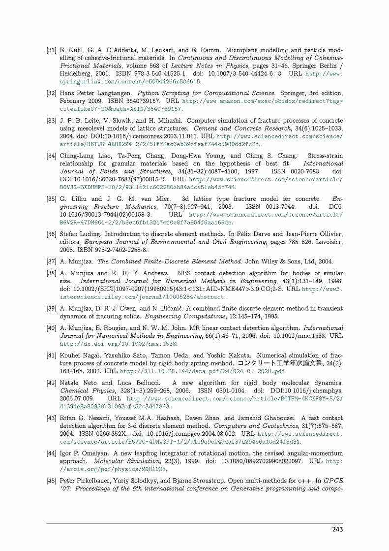
[31] E. Kuhl, G. A. D’Addetta, M. Leukart, and E. Ramm. Microplane modelling and particle mod-elling of cohesive-frictional materials. In Continuous and Discontinuous Modelling of Cohesive-Frictional Materials, volume 568 of Lecture Notes in Physics, pages 31–46. Springer Berlin /Heidelberg, 2001. ISBN 978-3-540-41525-1. doi: 10.1007/3-540-44424-6_3. URL http://www.springerlink.com/content/e50544266r506615.

[32] Hans Petter Langtangen. Python Scripting for Computational Science. Springer, 3rd edition,February 2009. ISBN 3540739157. URL http://www.amazon.com/exec/obidos/redirect?tag=citeulike07-20&path=ASIN/3540739157.

[33] J. P. B. Leite, V. Slowik, and H. Mihashi. Computer simulation of fracture processes of concreteusing mesolevel models of lattice structures. Cement and Concrete Research, 34(6):1025–1033,2004. doi: DOI:10.1016/j.cemconres.2003.11.011. URL http://www.sciencedirect.com/science/article/B6TWG-4B8X294-2/2/51f72ac6eb39cfeaf744c5980dd2fc2f.

[34] Ching-Lung Liao, Ta-Peng Chang, Dong-Hwa Young, and Ching S. Chang. Stress-strainrelationship for granular materials based on the hypothesis of best fit. InternationalJournal of Solids and Structures, 34(31–32):4087–4100, 1997. ISSN 0020-7683. doi:DOI:10.1016/S0020-7683(97)00015-2. URL http://www.sciencedirect.com/science/article/B6VJS-3XDHMP5-10/2/9311e21c602280eb84adca51eb4dc744.

[35] G. Lilliu and J. G. M. van Mier. 3d lattice type fracture model for concrete. En-gineering Fracture Mechanics, 70(7–8):927–941, 2003. ISSN 0013-7944. doi: DOI:10.1016/S0013-7944(02)00158-3. URL http://www.sciencedirect.com/science/article/B6V2R-47DM661-2/2/b3ec6fb13217ef0e8f7a854f6aa166de.

[36] Stefan Luding. Introduction to discrete element methods. In Félix Darve and Jean-Pierre Ollivier,editors, European Journal of Environmental and Civil Engineering, pages 785–826. Lavoisier,2008. ISBN 978-2-7462-2258-8.

[37] A. Munjiza. The Combined Finite-Discrete Element Method. John Wiley & Sons, Ltd, 2004.[38] A. Munjiza and K. R. F. Andrews. NBS contact detection algorithm for bodies of similar

size. International Journal for Numerical Methods in Engineering, 43(1):131–149, 1998.doi: 10.1002/(SICI)1097-0207(19980915)43:1<131::AID-NME447>3.0.CO;2-S. URL http://www3.interscience.wiley.com/journal/10005234/abstract.

[39] A. Munjiza, D. R. J. Owen, and N. Bićanić. A combined finite-discrete element method in transientdynamics of fracuring solids. Engineering Computations, 12:145–174, 1995.

[40] A. Munjiza, E. Rougier, and N. W. M. John. MR linear contact detection algorithm. InternationalJournal for Numerical Methods in Engineering, 66(1):46–71, 2006. doi: 10.1002/nme.1538. URLhttp://dx.doi.org/10.1002/nme.1538.

[41] Kouhei Nagai, Yasuhiko Sato, Tamon Ueda, and Yoshio Kakuta. Numerical simulation of frac-ture process of concrete model by rigid body spring method. コンクリート工学年次論文集, 24(2):163–168, 2002. URL http://211.10.28.144/data_pdf/24/024-01-2028.pdf.

[42] Natale Neto and Luca Bellucci. A new algorithm for rigid body molecular dynamics.Chemical Physics, 328(1–3):259–268, 2006. ISSN 0301-0104. doi: DOI:10.1016/j.chemphys.2006.07.009. URL http://www.sciencedirect.com/science/article/B6TFM-4KCXF8Y-5/2/d1394e8a82938b31093afa52c3d47863.

[43] Erfan G. Nezami, Youssef M.A. Hashash, Dawei Zhao, and Jamshid Ghaboussi. A fast contactdetection algorithm for 3-d discrete element method. Computers and Geotechnics, 31(7):575–587,2004. ISSN 0266-352X. doi: 10.1016/j.compgeo.2004.08.002. URL http://www.sciencedirect.com/science/article/B6V2C-4DMW3PT-1/2/d109e9e249daf37d294e6a10d24f8d31.

[44] Igor P. Omelyan. A new leapfrog integrator of rotational motion. the revised angular-momentumapproach. Molecular Simulation, 22(3), 1999. doi: 10.1080/08927029908022097. URL http://arxiv.org/pdf/physics/9901025.

[45] Peter Pirkelbauer, Yuriy Solodkyy, and Bjarne Stroustrup. Open multi-methods for c++. In GPCE’07: Proceedings of the 6th international conference on Generative programming and compo-

243

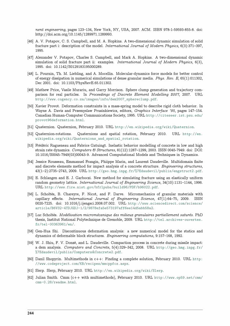
nent engineering, pages 123–134, New York, NY, USA, 2007. ACM. ISBN 978-1-59593-855-8. doi:http://doi.acm.org/10.1145/1289971.1289993.

[46] A. V. Potapov, C. S. Campbell, and M. A. Hopkins. A two-dimensional dynamic simulation of solidfracture part i: description of the model. International Journal of Modern Physics, 6(3):371–397,1995.

[47] Alexander V. Potapov, Charles S. Campbell, and Mark A. Hopkins. A two-dimensional dynamicsimulation of solid fracture part ii: examples. International Journal of Modern Physics, 6(3),1995. doi: 10.1142/S0129183195000289.

[48] L. Pournin, Th. M. Liebling, and A. Mocellin. Molecular-dynamics force models for better controlof energy dissipation in numerical simulations of dense granular media. Phys. Rev. E, 65(1):011302,Dec 2001. doi: 10.1103/PhysRevE.65.011302.

[49] Mathew Price, Vasile Murariu, and Garry Morrison. Sphere clump generation and trajectory com-parison for real particles. In Proceedings of Discrete Element Modelling 2007, 2007. URLhttp://www.cogency.co.za/images/info/dem2007_sphereclump.pdf.

[50] Xavier Provot. Deformation constraints in a mass-spring model to describe rigid cloth behavior. InWayne A. Davis and Przemyslaw Prusinkiewicz, editors, Graphics Interface ’95, pages 147–154.Canadian Human-Computer Communications Society, 1995. URL http://citeseer.ist.psu.edu/provot96deformation.html.

[51] Quaternion. Quaternion, February 2010. URL http://en.wikipedia.org/wiki/Quaternion.[52] Quaternion-rotations. Quaternions and spatial rotation, February 2010. URL http://en.

wikipedia.org/wiki/Quaternions_and_spatial_rotation.[53] Frédéric Ragueneau and Fabrice Gatuingt. Inelastic behavior modelling of concrete in low and high

strain rate dynamics. Computers & Structures, 81(12):1287–1299, 2003. ISSN 0045-7949. doi: DOI:10.1016/S0045-7949(03)00043-9. Advanced Computational Models and Techniques in Dynamics.

[54] Jessice Rousseau, Emmanuel Frangin, Phiippe Marin, and Laurent Daudeville. Multidomain finiteand discrete elements method for impact analysis of a concrete structure. Engineering structures,43(1–2):2735–2743, 2009. URL http://geo.hmg.inpg.fr/%7Edaudevil/publis/engstruct2.pdf.

[55] E. Schlangen and E. J. Garboczi. New method for simulating fracture using an elastically uniformrandom geometry lattice. International Journal of Engineering Science, 34(10):1131–1144, 1996.URL http://www.fire.nist.gov/bfrlpubs/build96/PDF/b96022.pdf.

[56] L. Scholtès, B. Chareyre, F. Nicot, and F. Darve. Micromechanics of granular materials withcapillary effects. International Journal of Engineering Science, 47(1):64–75, 2009. ISSN0020-7225. doi: 10.1016/j.ijengsci.2008.07.002. URL http://www.sciencedirect.com/science/article/B6V32-4TDJGDJ-1/2/9878efa5e573197aff6ee14d5abb58a2.

[57] Luc Scholtès. Modélisation micromécanique des milieux granulaires partiellement saturés. PhDthesis, Institut National Polytechnique de Grenoble, 2009. URL http://tel.archives-ouvertes.fr/tel-00363961/en/.

[58] Gen-Hua Shi. Discontinuous deformation analysis: a new numerical model for the statics anddynamics of deformable block structures. Engineering computations, 9:157–168, 1992.

[59] W. J. Shiu, F. V. Donzé, and L. Daudeville. Compaction process in concrete during missile impact:a dem analysis. Computers and Concrete, 5(4):329–342, 2008. URL http://geo.hmg.inpg.fr/%7Edaudevil/publis/Computers&Concrete2.pdf.

[60] Danil Shopyrin. Multimethods in c++: Finding a complete solution, February 2010. URL http://www.codeproject.com/KB/recipes/mmcppfcs.aspx.

[61] Slerp. Slerp, February 2010. URL http://en.wikipedia.org/wiki/Slerp.[62] Julian Smith. Cmm (c++ with multimethods), February 2010. URL http://www.op59.net/cmm/

cmm-0.28/readme.html.

244

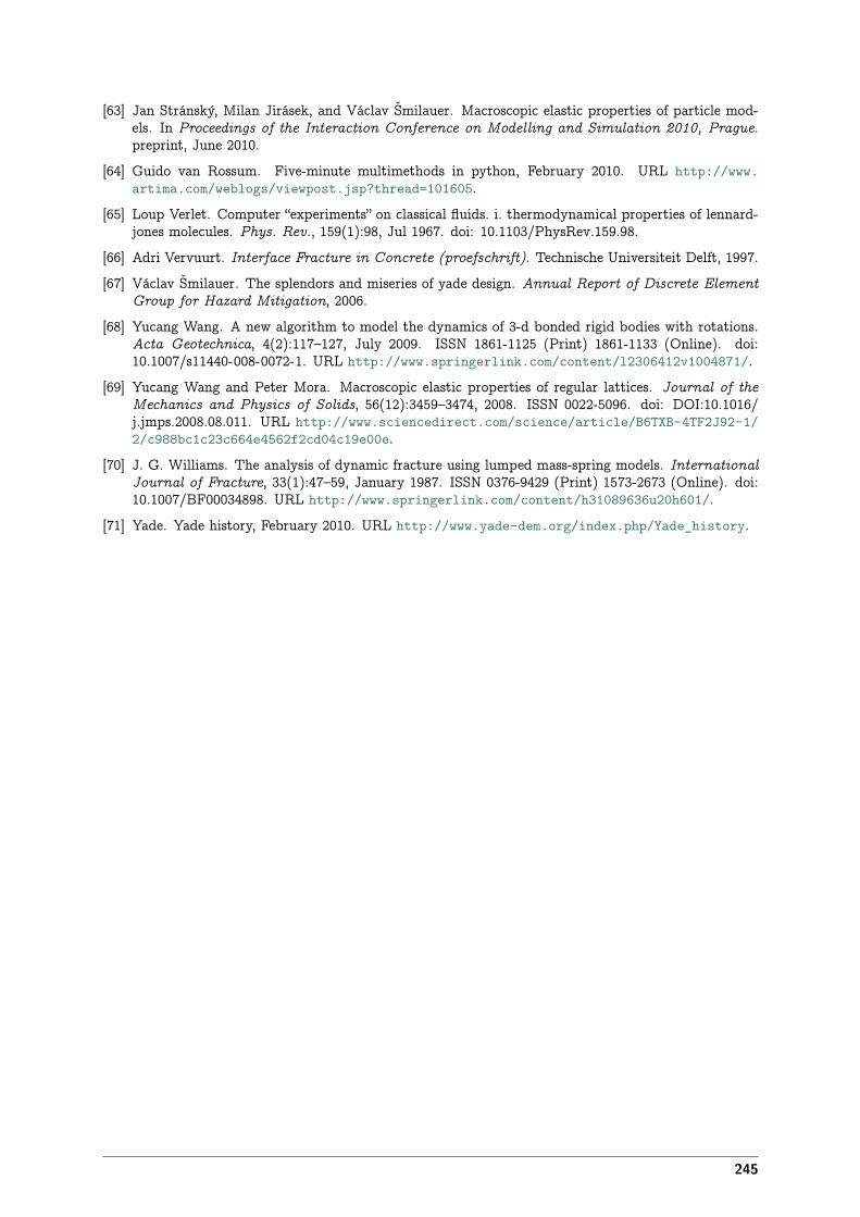
[63] Jan Stránský, Milan Jirásek, and Václav Šmilauer. Macroscopic elastic properties of particle mod-els. In Proceedings of the Interaction Conference on Modelling and Simulation 2010, Prague.preprint, June 2010.

[64] Guido van Rossum. Five-minute multimethods in python, February 2010. URL http://www.artima.com/weblogs/viewpost.jsp?thread=101605.

[65] Loup Verlet. Computer “experiments” on classical fluids. i. thermodynamical properties of lennard-jones molecules. Phys. Rev., 159(1):98, Jul 1967. doi: 10.1103/PhysRev.159.98.

[66] Adri Vervuurt. Interface Fracture in Concrete (proefschrift). Technische Universiteit Delft, 1997.[67] Václav Šmilauer. The splendors and miseries of yade design. Annual Report of Discrete Element

Group for Hazard Mitigation, 2006.[68] Yucang Wang. A new algorithm to model the dynamics of 3-d bonded rigid bodies with rotations.

Acta Geotechnica, 4(2):117–127, July 2009. ISSN 1861-1125 (Print) 1861-1133 (Online). doi:10.1007/s11440-008-0072-1. URL http://www.springerlink.com/content/l2306412v1004871/.

[69] Yucang Wang and Peter Mora. Macroscopic elastic properties of regular lattices. Journal of theMechanics and Physics of Solids, 56(12):3459–3474, 2008. ISSN 0022-5096. doi: DOI:10.1016/j.jmps.2008.08.011. URL http://www.sciencedirect.com/science/article/B6TXB-4TF2J92-1/2/c988bc1c23c664e4562f2cd04c19e00e.

[70] J. G. Williams. The analysis of dynamic fracture using lumped mass-spring models. InternationalJournal of Fracture, 33(1):47–59, January 1987. ISSN 0376-9429 (Print) 1573-2673 (Online). doi:10.1007/BF00034898. URL http://www.springerlink.com/content/h31089636u20h601/.

[71] Yade. Yade history, February 2010. URL http://www.yade-dem.org/index.php/Yade_history.

245