PHD_Final_exam_AlexandraM_Liguori

IntroductionPhD Work

ReferencesAppendices

Quantum Markovian Dynamics and Bipartite Entanglement

PhD student: Alexandra M. LiguoriSupervisor: Dr. Fabio Benatti

Departement of Theoretical Physics, University of Trieste

PhD defense,Trieste, March 26, 2010

A. Liguori Quantum Markovian Dynamics and Bipartite Entanglement



Outline

1 IntroductionTopicOpen Quantum Systems

2 PhD WorkEntanglement and entropy rates in open quantum systems

3 References

4 AppendicesMaster equation integrationMaximization




TopicOpen Quantum Systems

OPEN QUANTUM SYSTEMS

photons in cavities

atoms in external fields

molucules in biological systems

Usually environment’s effects on immersed subsystem are NEGATIVE, such asdecoherence.

POSITIVE EFFECTS of environmental NOISE on subsystem immersed within

generation of entanglement in separable states [e.g. Plenio,Huelga,PRL(2002); Benatti,Floreanini,Piani, PRL(2003); Benatti, A.M.L.,Nagy,JMP(2008)]

enhancement of transport properties [e.g. Plenio,Huelga, NJP(2008);Mohseni et al., JCP(2008)]





Topics of this PhD work

(1) OPEN QUANTUM SYSTEMS

systems whose interaction with theextrernal environment cannot beneglected

characterization of theenvironments’s action on thesystem within it through physicalquantities of the system itself

(2) ENTANGLEMENT IN OPENQUANTUM SYSTEMS

generation of entanglement via theenvironment in an initiallynon-entangled state of the system;

dynamical evolution of theentanglement and possibility of itsasymptotic persistence.





Focus of this PhD work

Discrete variables bipartite systems

S = SA + SB

↔ described by Hilbert space

H = HA ⊗HB , HA ≡ CdA , HB ≡ CdB

⇒ total Hilbert space of bipartite system

H ≡ CdA ⊗ CdB

of dimension d = dA × dB .





Open Quantum Systems

Systems where the interactions between the subsystem S and the externalenvironment E cannot be neglected.

State of S at time t = t ↔ irreversible time-evolution↔ master equation∂tt = L[t ]:

tracing away the environment degrees of freedom;

studying the evolution on a slow time-scale and neglecting fast decayingmemory effects (Markovian approximation) [Alicki,Lendi (’87); Gorini et al.,RMP(’76); Spohn, RMP(’80)].

⇒t = Γt [] ≡ etL [].

Standard weak or singular coupling limit techniques [Gorini et al., JMP(’76);Dumcke,Spohn, ZP(’79)]:

∂t

∂t= LH[t ] + LD [t ] = − i

~[H, t ] + LD [t ] ,

LD [t ] Kossakowski-Lindblad term





System S = 1 qubit

Kossakowski-Lindblad term:

L(1)

D [(t)] =3

∑

i,j=1

Kij

[

σj σi −12{σiσj , }

]

with σi , i = 1, 2, 3, the Pauli matrices.

⇒ 3 × 3 Kossakowski matrix K ≡ [Kij].

The constants Kij come from the Fourier transform of the bath correlationfunctions (see [Frigerio,Gorini, JMP(’76)]; Gorini,Kossakowski, JMP(’76))and form the so-called Kossakowski matrix K ≡ [Kij].

In order to guarantee full physical consistency, namely that Γt ⊗ idA bepositivity preserving on all states of the compound system S + A for anyinert ancilla A , Γt must be completely positive [Lindblad, CMP(’75)] and thisis equivalent to K being positive semidefinite [Gorini et al., JMP(’76);Lindblad, CMP(’76)].





System S = 2 qubits

Kossakowski-Lindblad term:

L(2)

D [(t)] =3

∑

i,j=1

(

Aij

[

(σj ⊗ I2) (σi ⊗ I2) −12{(σiσj ⊗ I2) , }

]

+Cij

[

(I2 ⊗ σj) (I2 ⊗ σi) −12{(I2 ⊗ σiσj) , }

]

+Bij

[

(σj ⊗ I2) (I2 ⊗ σi) −12{(σj ⊗ σi) , }

]

+B∗ji

[

(I2 ⊗ σj) (σi ⊗ I2) −12{(σi ⊗ σj) , }

])

with σi , i = 1, 2, 3, the Pauli matrices and I2 the 2 × 2 identity matrix

⇒ 6 × 6 Kossakowski matrix K =

(

A BB† C

)

3 × 3 matrices A = A †, C = C†

3 × 3 matrix B




Entanglement and entropy rates in open quantum systems

Entanglement in open quantum systems

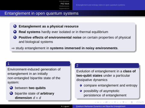
1 Entanglement as a physical resource2 Real systems hardly ever isolated or in thermal equilibrium3 Positive effects of environmental noise on certain properties of physical

and biological systems

⇒ study entanglement in systems immersed in noisy environments .

1

Environment-induced generation ofentanglement in an initiallynon-entangled bipartite state of thesystem:

1 between two qubits2 bipartite state of arbitrary

dimension d × d

2

Evolution of entanglement in a class oftwo-qubit states under a particulardissipative dynamics

compare entanglement and entropy

possibility of asymptoticpersistence of entanglement





Necessary and sufficient condition for entanglement to be generated at smalltimes in an initially separable pure state of two qubits Q = |ψ〉〈ψ| ⊗ |ϕ〉〈ϕ|only through the action of the common bath [Benatti, A.M.L.,Nagy, JMP(2008)]:

〈u|A |u〉〈v |CT |v〉 − |〈v |Re(B)|u〉|2 < 0

Kossakowski matrix

K =

(

A BB† C

)

vectors |u〉, |v〉: ui := 〈ψ|σi |ψ⊥〉 , vi := ǫi〈ϕ∗ |σi |ϕ∗⊥〉 = 〈ϕ⊥|σi |ϕ〉 ,σi , i = 1, 2, 3, Pauli matrices.






Dynamics of quantum systems in noisy environments↔ formalism ofnon-equilibrium thermodynamics ↔ change of entropy = entropy rate .

Connections between thermodynamics and entanglement, e.g. between secondlaw of thermodynamics and fundamental law of quantum information processing[Plenio,Vedral, CP(’98)]⇒ study behavior of entanglement in realistic systemsnot in equilibrium through a quantity defined as entanglement rate [Vedral,JP(2009)].

Minimize entropy rate,maximize entanglementrate

⇒ IDEA:

Study entanglement production and dynamicalevolution, and compare entanglement andentropy rates in open quantum systems.





Entropy rate

System in initial state in in contact with a bath with which it interacts driven intothe equilibrium thermal state T = e−βH/Z ⇒ total entropy change:∆St = ∆Sint + ∆Sext

Total entropy change in terms of relative entropy:

∆St := S(in ||T ) = Tr(in log in − in log T )

⇒

Entropy rate = time derivative of relative entropy:

σ = − ddt

(∆St) = −Tr( ddtin

)

(log in − log T ).





Entanglement rate

Compare entanglement rate with entropy rate⇒ relative entropy of entanglementto quantify entanglement [Vedral et al., PRL(’97); Vedral,Plenio, PRA(’98)]⇒

Relative entropy of entanglement

Relative entropy of evolved state (t) ≡ t with respect to the closest separablestate sep(t):

∆Et = infsep

S(

(t)||sep(t))

= infsep

Tr[

(t) log (t) − (t) log sep(t)]

⇒

Entanglement rate = time derivative of the relative entropy of entanglement:

σE =ddt

(∆Et) = infsep

Tr[

˙(t) log (t) − e log (t)−log sep(t) ˙sep(t)]

.





Conjecture [Vedral, JP(2009)]: for non-driven systems immersed in an externalbath the entanglement rate is always bounded by the entropy rate.

System: initial entangled state of 2 qubits

One qubit coupled to environment leading to dissipative evolution

Entanglement is dissipated, initial state becomes separable before steadystate is reached.

Entanglement rate (red line) vs. entropy rate (green line):

0.2 0.4 0.6 0.8 1.0

0.05

0.10

0.15

0.20

rosso: ÈΣ_EÈ verde: Σ





Our work

Previous conjecture and condition for environment-induced entanglementgeneration:

took different initial states of 2 qubits both immersed in a common externalbath

considered a particular dissipative evolution and integrated its masterequation

found asymptotic states

compared entanglement of initial states to entanglement of asymptotic states

studied entanglement rate and compared it to entropy rate generalizingprevious conjecture





System dynamics

2-qubit states immersed in a common external bath ⇒ Master eq.

∂tt = L[t ] = −i[H, t ] + LD [t ]

with

Hamiltonian H = ω2 Σ3

ω natural frequency of the system

Kossakowski-Lindblad term LD [t ] =∑3

i,j=1 Aij(ΣitΣj − 12 {ΣjΣi , t })

Σi := σi ⊗ I2 + I2 ⊗ σi

⇒ Kossakowski matrix K =

(

A AA A

)

[Aij ] ≡ A =

1 iγ 0−iγ 1 00 0 0

, with γ2 ≤ 1 for positivity of matrix A .





Initial states of 2 qubits of the form:

in = ain |1〉〈1| + din |2〉〈2| + bin |3〉〈3|+ cin |4〉〈4| =

ain 0 0 00 bin+cin

2bin−cin

2 00 bin−cin

2bin+cin

2 00 0 0 din

in the basis of eigenstates {|1〉〈1||, |2〉〈2|, |3〉〈3|, |4〉〈4}, with

|1〉 := |00〉, |2〉 := |11〉, |3〉 := 1√

2(|01〉+ |10〉), |4〉 := 1

√2(|01〉 − |10〉),





Evolved state:

t = at |1〉〈1| + dt |2〉〈2|+ bt |3〉〈3|+ ct |4〉〈4| =

at 0 0 00 bt +ct

2bt−ct

2 00 bt−ct

2bt +ct

2 00 0 0 dt

with at + bt + ct + dt = 1 form the condition Tr[t ] = 1 and ct = cin ≡ c.

Asymptotic states ∞ = limt→∞ t :

∞(c) =(1 − γ)2

3 + γ2(1 − c) |1〉〈1| + (1 + γ)2

3 + γ2(1 − c) |2〉〈2|

+(1 − γ2)

3 + γ2(1 − c) |3〉〈3| + c |4〉〈4| .

Compare amount of entanglement in initial and asymptotic states

Study entanglement rate and compare to entropy rate





Entropy rate σ calculated with respect to the asymptotic state of the dynamics,i.e. ∞ ≡ limt→∞ t .

Relative entropy of entanglement

∆E(t) = infsep

Tr[

(t) log (t) − (t) log sep(t)]

= −S(t) − supsep

Tr[

(t) log sep(t)]

= −S(t) − sup∈Sdiag

sep

(

at log x + dt log y + bt log u + ct log v)

at , bt , ct , dt coefficients in spectral decomposition of evolved state

x, y, u, v, coefficients of separable state diagonal in the same basis.





Various cases

initial state asymptotic state1 separable separable2 separable entangled3 entangled separable4 entangled entangled

The second case can take place if the entanglement generation condition

〈u|A |u〉〈v |CT |v〉 − |〈v |Re(B)|u〉|2 < 0

is fulfilled.

4

the asymptotic state is more entangled than the initial state;

the asymptotic state is less entangled than the initial state.





Compare amount of entanglement in the initial state with amount of entanglementin asymptotic state:

1 calculate and plot entropy of entanglement as function of time2 concurrence [Wootters, PRL(’98)]

C() := max {0, λ1 − λ2 − λ3 − λ4}

with λi , i = 1, 2, 3, 4, the square roots of the eigenvalues of ˆ taken indecreasing order, with ˆ := (σ2 ⊗ σ2)(σ2 ⊗ σ2).

In our case⇒ Concurrence:

C() = max

{

0, 2

(

|b − c |2−√

ad

)}

C(∞) = max

0,

∣

∣

∣

∣

1 − γ2 − 4c∣

∣

∣

∣

− 2(1 − γ2)(1 − c)

3 + γ2

.





Results

1) Initial pure separable state→ mixed separable state ∀t : conjecture holds.

= |1〉〈1|

∞ =(1 − γ)2

3 + γ2|1〉〈1| + (1 + γ)2

3 + γ2|2〉〈2| + (1 − γ2)

3 + γ2|3〉〈3|

C() = C(∞) = 0 ∀γ

No entanglement production ⇒ entropy rate as function of time:

0.1 0.2 0.3 0.4 0.5

2

4

6

8

10





2) Initial mixed separable state→ mixed entangled state: conjecture is violatedafter some time.

in =12(|3〉〈3| + |4〉〈4|) =

0 0 0 00 1/2 0 00 0 1/2 00 0 0 0

∞ =(1 − γ)2

2(3 + γ2)|1〉〈1| + (1 + γ)2

2(3 + γ2)|2〉〈2| + (1 − γ2)

2(3 + γ2)|3〉〈3| + 1

2|4〉〈4|

C() = 0 , C(∞) =2γ2

3 + γ2≥ 0

γ = 0.5⇒ C(∞) =2

13> 0





Entropy of entanglement:

0.2 0.4 0.6 0.8 1.0

0.01

0.02

0.03

0.04

0.05

Entanglement rate (continuous line) vs. entropy rate (dashed line):

0.2 0.4 0.6 0.8 1.0

0.05

0.10

0.15

0.20

0.25

0.30





3) Initial mixed entangled state→ mixed separable state: conjecture holds.

in =12|2〉〈2| + 1

10|3〉〈3| + 2

5|4〉〈4| = 1

10

0 0 0 00 2.5 −1.5 00 −1.5 2.5 00 0 0 5

,

∞ =3(1 − γ)2

5(3 + γ2)|1〉〈1| + 3(1 + γ)2

5(3 + γ2)|2〉〈2| + 3(1 − γ2)

5(3 + γ2)|3〉〈3| + 2

5|4〉〈4|

C() =35,

C(∞) = 0 for γ2 ≤ 311

C(∞) = 11γ2−35(3+γ2)

< 35 for 3

11 < γ2 ≤ 1

.

γ = 0.5⇒ C(∞) = 0






0.2 0.4 0.6 0.8 1.0

0.005

0.010

0.015

0.020

0.025

0.030


0.2 0.4 0.6 0.8 1.0

0.02

0.04

0.06

0.08

0.10

0.12





4) Initial mixed entangled state→ mixed entangled state with more or lessentanglement depending on the choice of γ.

in =3

10|2〉〈2| + 1

10|3〉〈3| + 3

5|4〉〈4| = 1

10

0 0 0 00 3.5 −2.5 00 −2.5 3.5 00 0 0 3

,

∞ =2(1 − γ)2

5(3 + γ2)|1〉〈1| + 2(1 + γ)2

5(3 + γ2)|2〉〈2| + 2(1 − γ2)

5(3 + γ2)|3〉〈3| + 3

5|4〉〈4|

C() =12, C(∞) =

3(1 + 3γ2)

5(3 + γ2)≥ 0 ∀γ





γ = 0.5⇒ C(∞) = 2165 <

12 ⇒ asymptotic state ∞ with less entanglement:

conjecture violated ∀ t .


0.2 0.4 0.6 0.8 1.0

0.02

0.04

0.06

0.08

0.10


0.2 0.4 0.6 0.8 1.0

0.02

0.04

0.06

0.08

0.10

0.12





γ = 0.9⇒ C(∞) = 10291905 >

12 ⇒ asymptotic state ∞ with more entanglement:

conjecture violated after some time.


0.0 0.2 0.4 0.6 0.80.090

0.095

0.100

0.105

0.110


0.2 0.4 0.6 0.8 1.0

0.01

0.02

0.03

0.04

0.05





Conclusions

New conjecture [Benatti,A. M. L.,Paluzzano, JPA(2010)]:

if the asymptotic state of the evolution is SEPARABLE , the previousconjecture is verified , i.e. the entanglement rate is always bounded by theentropy rate;

if the asymptotic state of the evolution is ENTANGLED , the previousconjecture fails , i.e. the entanglement rate is not bounded by the entropyrate, regardless of the fact whether the intial state is separable or entangled,and regardless of the fact whether the asymptotic state is more or lessentangled than the initial state.

Open questions

Study more general states with more general dissipative dynamics;

Find a general framework to explain the behaviour of entanglementproduction vs. entropy production we found in the open quantum systemswe considered.




[1]M. B. Plenio, S. Huelga, Phys. Rev. Lett. 88, 197901 (2002)[2]F. Benatti, R. Floreanini, M. Piani, Phys. Rev. Lett. 91, 070402 (2003)[3]F. Benatti, A. M. Liguori, A. Nagy, J. Math. Phys. 49, 042103 (2008)[4]M. B. Plenio, S. Huelga, New J. Phys. 10, 113019 (2008)[5]M. Mohseni et al., J. Chem. Phys. 129, 174106 (2008)[6]R. Alicki, K. Lendi, Lecture Notes in Physics, vol. 286, Springer-Verlag (1987)[7]V. Gorini et al., Rep. Math. Phys. 13, 149 (1976)[8]H. Spohn, Rev. Mod. Phys., 52, 569 (1980)[9]S. Gorini, A. Kossakowski, E. C. G. Sudarshan, J. Math. Phys. 17, 821 (1976)[10]R. Dumcke, H. Spohn, Z. Phys., B34, 419 (1979)[11]A. Frigerio, V. Gorini, J. Math. Phys. 17, 2123 (1976)[12]V. Gorini, A. Kossakowski, J. Math. Phys. 17, 1298 (1976)[13]G. Lindblad, Comm. Math. Phys. 40, 147-151 (1975)[14]M. B. Plenio, V. Vedral, Cont. Phys. 39, 431 (1998)[15]V. Vedral, Journal of Physics: Conference Series 143, 012010 (2009)[16]V. Vedral et al., Phys. Rev. Lett. 78, 2275 (1997)[17]V. Vedral, M. B. Plenio, Phys. Rev. A 57, 1619 (1998)[18]W. K. Wootters, Phys. Rev. Lett. 80, 2245 (1998)[19]F. Benatti, A. M. Liguori, G. Paluzzano, J. Phys. A: Math. Theor. 43, 045304(2010)




Master equation integrationMaximization

Master equation integration

Initial states of 2 qubits of the form:

in = ain |1〉〈1|+ din |2〉〈2| + bin |3〉〈3| + cin |4〉〈4| =

ain 0 0 00 bin+cin

2bin−cin

2 00 bin−cin

2bin+cin

2 00 0 0 din

in the basis of eigenstates {|1〉〈1||, |2〉〈2|, |3〉〈3|, |4〉〈4}, with

|1〉 := |00〉, |2〉 := |11〉, |3〉 := 1√

2(|01〉+ |10〉), |4〉 := 1

√2(|01〉 − |10〉).





Hamiltonian H = ω2 Σ3

Kossakowski-Lindblad term LD [t ] =∑3

i,j=1 Aij(ΣitΣj − 12 {ΣjΣi , t })

Σi := σi ⊗ I2 + I2 ⊗ σi

⇒ Kossakowski matrix

[Aij] ≡ A =

1 iγ 0−iγ 1 00 0 0

⇒ eigenvalues of A : 1 + γ, 1 − γ, 0⇒ diagonalizing: A = UDU†, with

D = diag[1 + γ, 1 − γ, 0], U =

1/√

2 1/√

2 0−i/√

2 i/√

2 00 0 1





⇒ action of the Kossakowski-Lindblad term on the state of the two qubits:

LD [t ] =3

∑

i,j=1

(UDU†)ij

(

ΣitΣj −12{ΣjΣi , t }

)

=3

∑

i,j=1

3∑

l=1

alUilU∗jl

(

ΣitΣj −12{ΣjΣi , t }

)

= 2(1 + γ)(

Σ−tΣ+ −12{Σ+Σ−, t }

)

+ 2(1 − γ)(

Σ+tΣ− −12{Σ−Σ+, t }

)

with Σ± := 12 (Σ1 ± iΣ2).

For the basis states:

Σ+|1〉 = 0Σ+|2〉 =

√2|3〉

Σ+|3〉 =√

2|1〉Σ+|4〉 = 0

,

Σ−|1〉 =√

2|3〉Σ−|2〉 = 0Σ−|3〉 =

√2|2〉

Σ−|4〉 = 0





Interaction picture :def. state ˜t := e iHtt e−iHt ⇒ operators

Σ±(t) := e iHtΣ±e−iHt = e±iωtΣ± ⇒

ddt

Σ± = i[H,Σ±] = ±iωΣ±

⇒ Master equation for ˜t :

˙t = −i[H, ˜t ] + LD [ ˜t ] = e iHtLD [˜t ]e

−iHt (1)

= 2(1 + γ)(

e iHtΣ−e−iHt ˜t e iHtΣ+e−iHt − 12

e iHt {Σ+Σ−, e−iHt ˜t e iHt }e−iHt)

+ 2(1 − γ)(

e iHtΣ+e−iHt ˜t eiHtΣ−e

−iHt − 12

e iHt {Σ−Σ+, e−iHt ˜t e

iHt }e−iHt)

= 2(1 + γ)(

Σ− ˜tΣ+ −12{Σ+Σ−, ˜t }

)

+ 2(1 − γ)(

Σ+ ˜tΣ− −12{Σ−Σ+, ˜t }

)

,





Representing

˜t =4

∑

i,j=1

ρij(t)|i〉〈j|

in terms of the orthonormal basis {|1〉〈1|, |2〉〈2|, |3〉〈3|, |4〉〈4|}

Integrating (1)

⇒ ˜t = ρ11(t)|1〉〈1|+ ρ33(t)|3〉〈3| + ρ44(t)|4〉〈4| + ρ22(t)|2〉〈2|.

Note

˜t is diagonal with respect to the orthonormal basis {|1〉〈1|, |2〉〈2|, |3〉〈3|, |4〉〈4|}.





⇒ explicit form for the evolution of the initial state in:

(t) ≡ t := e−iHt ˜teiHt = e−i ω2 Σ3 t ˜t e

i ω2 Σ3 t

= e−i ω2 Σ3 t |1〉〈1|e i ω2 Σ3 t + e−i ω2 Σ3 t |2〉〈2|e i ω2 Σ3 t

+ e−i ω2 Σ3 t |3〉〈3|e i ω2 Σ3 t + e−i ω2 Σ3 t |4〉〈4|e i ω2 Σ3 t

≡ ˜t

⇒ t ≡ exp(LD [in])

and ρ11 = at , ρ22 = dt , ρ33 = bt , ρ44 = ct = cin.

Note

The last equality is due to the fact that ˜t only contains diagonal terms and theexponentials e±i ω2 Σ3 t thus cancel out in each term of the above sum (this wouldnot be the case for a generic 2-qubit state with spectral decomposition =

∑4i,j=1 ij |i〉〈j|).





Derive the equations :

ρ11 = −4(1 + γ)ρ11 + 4(1 − γ)ρ33 , ρ12 = −4ρ12

ρ13 = −2(3 + γ)ρ13 + 4(1 − γ)ρ32 , ρ14 = −2(1 + γ)ρ14

ρ22 = −4(1 − γ)ρ22 + 4(1 + γ)ρ33 , ρ23 = −2(3 − γ)ρ23 + 4(1 + γ)ρ31

ρ33 = 4(1 + γ)ρ11 + 4(1 − γ)ρ22 − 8ρ33 , ρ24 = −2(1 − γ)ρ24

ρ34 = −4ρ34 , ρ44 = 0 ,

plus the complex conjugated equations for ρij , i , j.⇒ Solutions:

ρ12(t) = ρ12 e−4t

ρ13(t) = 0

ρ14(t) = ρ14 e−2(1+γ)t

ρ24(t) = ρ24 e−2(1−γ)t

ρ32(t) = 0

ρ34(t) = ρ34 e−4t

ρ44(t) = ρ44 .





ρ11(t) =(1 − γ)2

3 + γ2R +

√

1 − γ2(1 + γ)2ρ11 − 2(1 − γ)ρ22 + (1 + γ)2ρ33

(1 + γ)(3 + γ2)E−(t)

+2(1 + γ)ρ11 − (1 − γ)2(ρ22 + ρ33)

3 + γ2E+(t)

ρ22(t) =(1 + γ)2

3 + γ2R −

√

1 − γ22(1 + γ)ρ11 − (1 − γ)2(ρ22 + ρ33)

(1 − γ)(3 + γ2)E−(t)

− (1 + γ)2ρ11 − 2(1 + γ)ρ22 + (1 + γ)2ρ33

3 + γ2E+(t)

ρ33(t) =(1 − γ2)

3 + γ2R +

√

1 − γ2(1 + γ)3ρ11 + (1 − γ)3ρ22 − 2(1 − γ2)ρ33

(3 + γ2)(1 − γ2)E−(t)

+2(1 + γ2)ρ33 − (1 − γ2)(ρ11 + ρ22)

3 + γ2E+(t) ,

where R = ρ11 + ρ22 + ρ33 = ρ11(t) + ρ22(t) + ρ33(t)

E±(t) = e−8t

{

cosh 4t√

1 − γ2

sinh 4t√

1 − γ2, F±(t) = e−8t

{

cosh 2t√

4 − 3γ2

sinh 2t√

4 − 3γ2.





Maximization

AIM: Maximize Tr[(t) log sep(t)] over the set of separablestates.

Spectral decomposition of (t) =∑4

i=1 ri(t)|i〉〈i|separable state sep =

∑4j=1 sj |sj〉〈sj |

⇒ Tr[(t) log sep] =4

∑

i=1

ri(t)〈i| log sep |i〉 =4

∑

i=1

ri(t)4

∑

j=1

|〈i|sj〉|2 log(sj)

≤4

∑

i=1

ri(t) log( 4∑

j=1

sj |〈i|sj〉|2)

=4

∑

i=1

ri(t) log〈i|sep |i〉 = Tr(

(t) log Π[sep ])

,

Π[sep ] :=∑4

i=1 |i〉〈i|sep |i〉〈i|,∑4

j=1 |〈i|sj〉|2 = 1,inequality in second line from convexity of logarithm.





(1)

Tr[(t) log sep] ≤ Tr(

(t) log Π[sep ])

⇒supsep

Tr[(t) log sep] ≤ supsepTr

(

(t) log Π[sep ])

(2)

separable ⇒ Π[] separable for any separable state ⇒ Π[·] maps separable states into separable states⇒ supsep

Tr(

(t) log Π[sep ])

≤ supsepTr[(t) log sep]

Compute

supsep

Tr[(t) log sep]

MaximizeTr

(

(t) log Π[sep ])

with respect to the separable state ˜sep ≡ Π[sep ]

sep =4

∑

i=1

si |i〉〈i|





In this case the separable state can be written explicitly as

sep = x |1〉〈1| + u|3〉〈3| + v |4〉〈4|+ y |2〉〈2| =

x 0 0 00 u+v

2u−v

2 00 u−v

2u+v

2 00 0 0 y

, (2)

with x + u + v + y = 1, and(

u−v2

)2≤ xy from the condition of non-negativity of

the partial transpose to ensure the separability of sep .

Maximize Tr(

(t) log Π[sep ])

with the explicit expression (2) for sep :

1 define the function f(x, y, u, v) := a log x + d log y + b log u + c log vat ≡ a, bt ≡ b, ct ≡ c, dt ≡ d coefficients in spectral decomposition of evolvedstate

2 maximize this function with the constraint λ(x + y + u + v − 1), from thecondition x + u + v + y = 1 on the trace of sep .





Set the partial derivatives of function f with respect to x, y, u, v to zero⇒ obtainthe conditions:

a = −λxd = −λyb = −λuc = −λv

Together with the conditions a + b + c + d = 1 and x + u + v + y = 1⇒ λ = −1⇒ a = x, d = y, b = u, c = v.

1 (x, y, u, v) are the coefficients of a separable state while (a, d, b, c, ) arethose of a generic state which could be entangled

2 the set of separable states is compact

(1) and (2)⇒ the maximum must lie on the border of this set of separable states,

i.e. we must have(

u−v2

)2= xy ⇒ u± =

1−(√

x∓√y)2

2 , v± =1−(√

x±√y)2

2





⇒ function to be maximized

f(x, y) = a log x + d log y + b log(1 − (

√x ∓ √y)2

2

)

+ c log(1 − (

√x ± √y)2

2

)

.

⇒ Solutions:y = x − a + d

and

x =1

(8(−1 + b)(a + b + d)){−a3 − d(−1 + 2b + d)2 + a2(−6 + 4b + d)

+ a(−1 + 4(−1 + b) + d2) + [(−1 + a + 2b + d)2(a4 + 2a3(−1 + 2b − 2d)

+ d2(−1 + 2b + d)2 + a2(1 + 4b2 + 2d + 6d2 − 4b(1 + d))

+ 2ad(1 + d − 2(2b(−1 + b) + bd + d2)))]1/2}.


PHD_Final_exam_AlexandraM_Liguori

Science

Transcript of PHD_Final_exam_AlexandraM_Liguori