PhD. Thesis in Physics and Astrophysics
107
Transcript of PhD. Thesis in Physics and Astrophysics


PhD. Thesis in Physics and Astrophysics
XXX CYCLE FIS/03
Exploring quantum phase slips in 1D bosonic
systems
Presented by
Simona Scaffidi Abbate
Supervisor: Chiara D’Errico
Supervisor : Giovanni Modugno
Coordinator: Raffaello D’alessandro

Alla mia famiglia, per avermi supportato
A Marisa, per avermi sopportato
A Jacopo e Simone, per avermi fatto sempre sorridere
A Marco, per avermi incoraggiato e per avere sempre avuto fiducia in me

Contents
Introduction 1
1 Bose-Einstein Condensate 5
1.1 Non-interacting particles: ideal BEC . . . . . . . . . . . . . . . . . . . . . . . . 7
1.2 Interacting particles . . . . . . . . . . . . . . . . . . . . . . . . . . . . . . . . . . 10
1.3 Feshbach resonances . . . . . . . . . . . . . . . . . . . . . . . . . . . . . . . . . 14
1.4 Optical dipole potentials: red detuned trap . . . . . . . . . . . . . . . . . . . . 17
1.5 Optical lattices . . . . . . . . . . . . . . . . . . . . . . . . . . . . . . . . . . . . 19
1.5.1 Bloch Theorem . . . . . . . . . . . . . . . . . . . . . . . . . . . . . . . . 20
1.5.2 Semi-Classical Dynamics . . . . . . . . . . . . . . . . . . . . . . . . . . . 23
2 Physics of 1D BEC 25
2.1 1D Quasi-condensate . . . . . . . . . . . . . . . . . . . . . . . . . . . . . . . . . 25
2.2 Experimental 1D system . . . . . . . . . . . . . . . . . . . . . . . . . . . . . . . 27
2.3 Momentum distribution and correlation . . . . . . . . . . . . . . . . . . . . . . . 28
2.4 Theoretical model for 1D systems . . . . . . . . . . . . . . . . . . . . . . . . . . 30
2.4.1 Luttinger Liquid . . . . . . . . . . . . . . . . . . . . . . . . . . . . . . . 30
2.4.2 Lieb-Liniger Model . . . . . . . . . . . . . . . . . . . . . . . . . . . . . . 32
2.4.3 Bose-Hubbard Model . . . . . . . . . . . . . . . . . . . . . . . . . . . . . 33
2.4.4 Superfluid and Mott Insulator . . . . . . . . . . . . . . . . . . . . . . . . 35
2.5 Sine-Gordon Model . . . . . . . . . . . . . . . . . . . . . . . . . . . . . . . . . . 39
3 Phase Slips in one dimensional systems 41
3.1 Phase slips in superconductors . . . . . . . . . . . . . . . . . . . . . . . . . . . . 41
3.2 Quantum phase slips in superfluids . . . . . . . . . . . . . . . . . . . . . . . . . 46
3.2.1 Quantum phase slips in one-dimensional superfluids in a periodic poten-
tial: theorethical model in the Bose-Hubbard regime. . . . . . . . . . . . 46
i
ii CONTENTS
4 Exploring quantum phase slips in 1D bosonic systems 53
4.1 Experimental procedure . . . . . . . . . . . . . . . . . . . . . . . . . . . . . . . 53
4.2 Realization of 1D systems . . . . . . . . . . . . . . . . . . . . . . . . . . . . . . 56
4.3 Exciting the 1D motion . . . . . . . . . . . . . . . . . . . . . . . . . . . . . . . . 59
4.4 Dissipation in the presence of oscillations . . . . . . . . . . . . . . . . . . . . . . 60
4.4.1 Dynamical instability . . . . . . . . . . . . . . . . . . . . . . . . . . . . . 61
4.4.2 Observation of velocity-dependent quantum phase slips . . . . . . . . . . 65
4.4.3 Comparison between our experimental results and the theoretical model
of thermally activated phase slips of one-dimensional Bose gases in the
Sine Gordon limit. . . . . . . . . . . . . . . . . . . . . . . . . . . . . . . 71
4.5 Dissipation at constant velocity . . . . . . . . . . . . . . . . . . . . . . . . . . . 74
4.5.1 Shallow lattice . . . . . . . . . . . . . . . . . . . . . . . . . . . . . . . . 76
4.5.2 Deep lattice . . . . . . . . . . . . . . . . . . . . . . . . . . . . . . . . . . 79
Conclusions 81
A Disordered systems 85
B Landau instability 91
References . . . . . . . . . . . . . . . . . . . . . . . . . . . . . . . . . . . . . . . . . . 95
*

Introduction
Phase slips, i.e. phase fluctuations of the superfluid order parameter, are the primary excita-
tions of one-dimensional superfluids and superconductors, in the presence of an obstacle for the
superflow and supercurrent [1, 2, 3, 4, 5, 6, 7]. These excitations are particularly abundant in
one-dimensional systems because of their fragility and vulnerability to the presence of pertur-
bations and fluctuations compared to higher dimensional systems. The phenomenon of phase
slips has been originally studied in the field of superconductors, and only recently it has been
investigated also in the field of ultracold quantum gases, which are offering an unprecedented
opportunity of exploring important quantum phenomena. They are, in fact, very versatile and
powerful tools and good candidates to be suitable quantum simulators of several phenomena
concerning condensed matter, superfluidity and superconductivity, thanks to the control and
manipulation of key properties such as dimensionality and interactions that can be changed by
using optical lattices and Feshbach resonances [8].
The first theoretical proposal for the phase-slip phenomenon was made by Little in 1967
[1] in order to describe the finite resistance of thin wires below the critical temperature for
superconductivity. He supposed that each segment of a thin wire has a finite probability to
become, for a very short time, a normal conductor. Due to these fluctuations, which are
originated by thermal effects, the persistent current is disrupted and a non-zero resistance
in the wire arises. In this situation, the excitations are known as thermally activated phase
slips (TAPS). However, the resistance may remain finite also at zero temperature, due to the
presence of quantum phase slips (QPS), which may occur via quantum tunnelling events.
Phase slips, both thermal and quantum, have been deeply investigated, both from a theo-
retical and experimental point of view, in different condensed-matter systems. In particular,
they have been observed in superconducting nanowires [11, 9, 10, 12, 13, 14] and Josephson
junction arrays [15].
The phenomenon of phase slips became of interest also in the field of superfluids based
on ultracold quantum gases. This kind of systems, in fact, gives the possibility to investigate
1
2 CONTENTS
aspects of phase slips that are not accessible in other systems, thanks to their extreme tunability.
For example, by tuning the interactions among the particles of the Bose-Einstein condensate
(BEC) thanks to Feshbach resonances [16, 17], it is possible to understand if the interactions
can modify the nucleation rate of phase slips or if they can influence the generation of quantum
phase slips rather than the nucleation of thermally activated ones. In condensed-matter physics,
in fact, tuning the interactions between the Cooper pairs is difficult to achieve. Moreover, it is
possible to study the phenomenon of phase slips also in one dimensional system with different
geometry. Recently, both theory and experiments investigated the phase slips mechanisms not
only in a one-dimensional superfluids [5] but also in a ring geometry [7].
In the case of ultracold quantum gases the presence of phase slips induces a finite dissipa-
tion, which is the analogous of the resistance in condensed matter systems. So, the goal in
the presence of BEC is to study the dissipation induced by phase slips as a function of the
interaction, temperature and velocity. Despite several theoretical models concerning the phe-
nomenon of phase slips in ultracold quantum gases have been made, an experimental exhaustive
picture of QPS in ultracold superfluids has not been obtained until few years ago. The first
signatures of QPS obtained so far are the observation of a regime of temperature-independent
dissipation for a Bose-Einstein condensate in a 3D optical lattice in the group of Brian DeMarco
[18], and our recent observation of velocity-dependent dissipation in one dimensional lattices
(1D) [19, 20, 21]. Theoretical studies that attempt to reproduce the experiments are underway
[22, 23].
As in the case of condensed matter systems, also in the presence of ultracold quantum gases
there are experimental obstacles, which make the observation of the phase slips difficult. For
example, the occurrence of the Mott insulating phase [24] prevents the observation of phase
slips in the strongly interacting regime. In fact, when the system is a Mott insulator the
superfluidity of the system, which is the key ingredient to study how fluctuations affect the
transport properties of the superfluid, is lost. Moreover, it is also difficult to explore a wide
range of currents, i.e. superfluid velocities, due to the occurrence of two different dissipation
phenomena: the Landau instability and dynamical instability. The first phenomenon is related
to the Landau’s criterion of the superfluidity [25, 26], i.e. if the system flows slower than a
critical velocity vc, which correspond to the sound velocity, no excitations can be created and
the system does not dissipate. As soon as the system exceeds the critical velocity, phonons will
be emitted, inducing thus a energy lost for the superfluid. The latter phenomenon is related to
the divergence of the phase-slip nucleation rate: if the system velocity is larger than a critical
velocity for the dynamical instability, the system enters a dynamically unstable regime driven

CONTENTS 3
by a divergence of the phase slip rate and strongly dissipates.
In order to observe the presence of QPS and to study how this kind of fluctuations modifies
the behaviour of our system, we performed transport measurements by using a trap oscillation
technique in the presence of a 1D optical lattice, and we studied the time evolution of the
momentum of the system. We observe two different behaviours depending on the momentum
reached during the oscillation. For momenta smaller than the critical momentum for the dy-
namical instability we observe that our system oscillates with a damping due to the presence of
phase slips. For large momenta we observe instead an overdamped motion, which we attribute
to the occurrence of the dynamical instability that can be described in term of a divergence of
the phase-slips rate at the critical velocity for the dynamical instability. In the first part of my
thesis, I will show the experimental results regarding these two different phenomena, obtained
by exciting the sloshing motion of the system for different values of interactions, velocities and
temperature. In the second part of my thesis, I will focus the attention on transport mea-
surements performed at constant velocity. By employing this new experimental technique, we
can overcome some experimental limits occurring when we excite the sloshing motion of the
system, and we can investigate the system dissipation in the regime of low velocity and strong
interactions. In both cases of weak and deep 1D optical lattice, we observe a finite dissipation,
not only in the superfluid regime, but also in the Mott insulating one. We attribute this dissi-
pation when the system is in the Mott insulating regime to the nucleation of phase slips of the
residual superfluid phase, which is due to the fact that we have an inhomogeneous system.
The presentation of the thesis is organized as follows. In the first chapter I will introduce the
main instruments related to the physics of BECs. I will discuss the Bose Einstein condensation
theoretical model and I will focus the attention on the experimental techniques employed to
independently control interactions and dimensionality, i.e. Feshbach resonances and optical
lattices. In the end of this chapter I will talk about the physics of a particle in an optical
lattice.
In the second chapter, I will focus the attention on one-dimensional systems. Initially I
will describe the importance and the basic features of one-dimensional systems. Then I will
introduce the theoretical frameworks of a one dimensional systems in the presence of an optical
lattice, i.e. the Bose Hubbard model and the Sine Gordon ones. I will show that depending
on the competition between the interaction energy and the tunnelling one, the systems may
behave as an insulator rather than a superfluid.
The third chapter concerns the phenomenon of phase slips in 1D systems. First I will
introduce the phenomenon in superconductors and I will show both the theoretical and the
4 CONTENTS
experimental results regarding thermally activated phase slips and quantum ones. Then I will
briefly discuss the first experimental signatures of QPS in superfluids and I will focus the
attention on the theoretical model of phase slips in 1D atomic superfluids.
The last chapter is the core of my thesis, and it is dedicated to our experimental results
regarding the observation of phase slips (both quantum and thermal). In the first part I will
briefly describe how we realize the 1D superfluids by starting from a three-dimensional 39K
BEC. Then, I will initially focus the attention on the transport measurements performed by
using the trap oscillation technique, and subsequently I will describe the transport measure-
ments performed at constant velocity.

Chapter 1
Bose-Einstein Condensate
Bose-Einstein Condensates (BECs) are extremely versatile and powerful tools which can be
employed in order to investigate quantum problems related to different branches of physics.
The phenomenon of BEC occurs when a high fraction of bosonic particles in thermal equi-
librium occupies the same single particle ground state. In this situation, they are observable
macroscopic objects behaving according to the laws of quantum mechanics.
The phenomenon of BEC was predicted in 1924 by Bose and Einstein [27, 28] and it was
experimentally observed for the first time in 1995, almost simultaneously in three different
groups [29, 30, 31] which employed Alkali atoms.
In order to better understand the Bose Einstein condensation, let us consider a gas of N
bosons in the continuum confined in a 3-dimensional box with volume V , which in thermal
equilibrium are characterized by a density n = d−1/3, being d the mean distance between
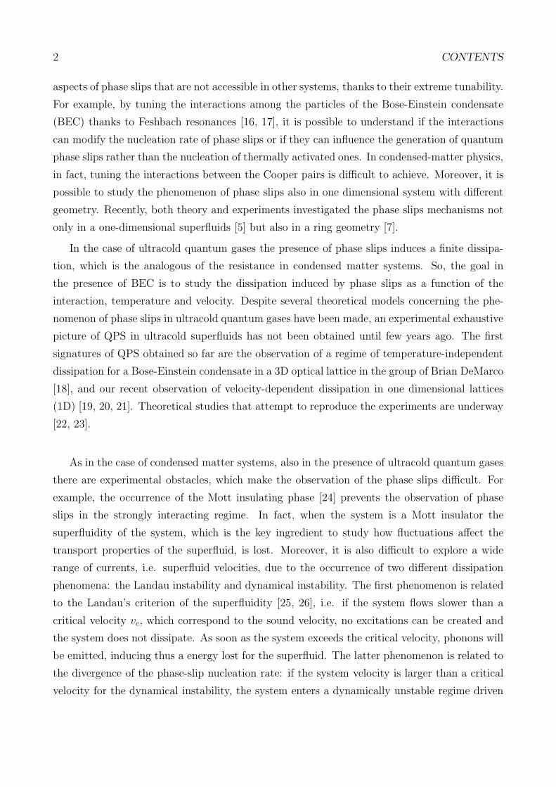
Figure 1.1: Phase transition to the BEC. (a) When T ≫ Tc, the distance between the particles, d , islarge than the De Broglie wavelength λDB and the particles obey to the Boltzmann statistics. (b) Bydecreasing the temperature the quantum nature of the particles must be taken into account and theymust be described by using a wave function. (c) At T ≃ Tc the wave functions start overlapping and amacroscopic number of particles occupy the lowest-energy quantum state giving rise to the BEC. (d)At T = 0, all particles are in the same quantum state, giving rise at a pure BEC without any thermalcomponent
5
6 CHAPTER 1. BOSE-EINSTEIN CONDENSATE
the particles, and by a thermal velocity v. At high temperature, they can be considered as
distinguishable point-like particles, obeying to the Boltzmann statistics (Fig.1.1a). Decreasing
the temperature, the quantum nature of the particles must be taken into account and they
must be described by using a wave function, which is symmetric under interchange of any pair
of particle, due to the bosonic nature of the particles (Fig.1.1b). In this situation, the spatial
extension of a particle can be suitably described in terms of its De Broglie wavelength
λDB =
√
2π~2
mkBT(1.1)
where m is the particle mass, T the temperature and ~ and kB are, respectively, the Planck
and the Boltzmann constants. Decreasing the temperature below a critical temperature Tc,
the De Broglie wavelength becomes of the order of the mean distance between the particles,
i.e.(
VN
)1/3 ≈ λDB, the wave functions start overlapping, the particles cannot be considered
distinguishable any longer and a phase transition occurs. In particular, a macroscopic number of
particles occupies the lowest-energy quantum state , giving rise to the BEC (Fig.1.1c). Ideally,
at T = 0, all particles are in the same quantum state, giving rise at a pure BEC without any
thermal component (Fig.1.1d). At the phase transition, n and T are related via
nλ3DB = 2.612, (1.2)
where nλ3DB is the phase-space density, which is defined as the number of atoms in a box
with a volume equal to λ3DB. In this way, depending on the value of the phase-space density, it is
possible to know if the system behaves according to the laws of quantum or classical mechanics.
For example, a system of 87Rb at T = 300 K and P = 1 Atm, behaves according to the laws
of classical mechanics, due to the fact that the phase-space density nλ3DB ≈ 10−8 is eight order
of magnitude smaller than the phase-space density at the phase transition. In order to reach
the BEC phase, one can act on the phase-space density either by increasing the density or
decreasing the temperature. However, by increasing the density, the probability of three-body
recombination increases as well and this results in an increase of atoms losses. In fact, when
three atoms are close to each other, two of them may form a dimer, which is usually in an
excited vibrational state, whereas the third atom carries away the released energy. Due to the
fact that this energy is much larger than the typical depth of the trap confining the atoms, the
three atoms are lost and the system is subject to heating.
In addition, not only the increase of the density but also the decrease of the temperature
gives rise to a problem. By decreasing the temperature, in fact, all the known interacting
systems undergo a phase transition to the solid phase, with the exception of the helium. Both
1.1. NON-INTERACTING PARTICLES: IDEAL BEC 7
problems can be solved by employing dilute gases which are defined as systems with a density
many thousand times more dilute than air, where the mean interparticle distance is much
greater than the scattering length a for s-wave collisions, i.e.
n ≪ 1
a3. (1.3)
In this condition, the probability for three-body collisions to occur is severely reduced and
at the same time the samples can be cooled down to very low temperatures (of the order of 1µK
or less) due to the fact that the still probable two-body collisions keep the gas in a metastable
state, avoiding the transition to the solid phase.
1.1 Non-interacting particles: ideal BEC
Let’s consider an ideal system of non interacting bosons at the thermodynamic equilibrium. As
it is well known, the mean occupation number of bosons in the single-particle state ν is given
by the Bose-Einstein distribution [27, 28, 32]
f(ǫν) =1
e(ǫν−µ)/kBT − 1(1.4)
where T is the temperature, ǫν is the energy of the νth single particle energy state and µ
is the chemical potential. The latter depends on the total number of particles N and on the
temperature T via the normalization condition, which imposes that the total number of particles
must be equal to the sum of the occupancies of the individual levels. At high temperature, the
chemical potential is much smaller than the ground state energy ǫmin, due to the fact that the
mean occupation number of the single-particle state is less than unity, and the Bose statistics eq.
1.4 reduces to the Maxwell-Boltzmann statistics. By decreasing the temperature, the chemical
potential increases as well as the mean occupation numbers. However, µ cannot exceed the
ground state energy, due to the fact that if µ > ǫmin, f(ǫν) becomes negative and loses its
physical meaning. Consequently, µ must be always lower than ǫmin and the mean occupation
number of any excited single-particle state is superiorly limited by the value 1e(ǫν−ǫmin)/kBT−1
.
In general, at a fixed temperature T , the constant total number of particles Ntot is given
via Ntot = Nexc + N0 where Nexc is the number of particles in the excited state and N0 is the
number of particles remaining in the ground state. If the number of particles in the ground
state is arbitrarily large, the system has a BEC and this happens when the chemical potential
approaches the ground state energy. The highest temperature at which the ground state is
macroscopically occupied is known as Bose Einstein transition temperature Tc and it is defined

8 CHAPTER 1. BOSE-EINSTEIN CONDENSATE
via
Nexct(Tc, µ = ǫmin) = Ntot (1.5)
More in detail, at the transition Next is given by the equation
Nexct(Tc, µ = 0) = Ntot =
∞∫
0
dǫg(ǫ)1
e(ǫ)/kBTc − 1(1.6)
where the ground state energy ǫmin = 01. In the Eq. 1.6 g(ǫ) is the density of the state,
defined as g(ǫ) = dG(ǫ)dǫ
where G(ǫ) is the total number of states with energy less than ǫ.
Depending on the system boundary condition, the density of the states depends differently on
the energy. In particular, in the ideal situation of a non-interacting d-dimensional system in
thermal equilibrium and at zero temperature, the density of state depends on the energy via
g(ǫ) ∝ ǫd/2−1, which implies that in a two-dimensional system the density of the states does
not depend on the energy. Instead, in the situation of non-interacting identical bosons in a d-
dimensional harmonic confining potential V (r) = 12m
d∑
i=1
ω2i x
2i2 with frequency ωi, the density of
states depends on the energy via g(ǫ) = ǫd−1
(d−1)∏
i~ωi
. As a consequence, the critical temperature
behaves differently depending on the system dimensionality. In general it can be written as
kTc =N
1/αtot
[CαΓ(α)ζ(α)]1/α. (1.7)
Here Γ(α) and ζ(α) are, respectively, the gamma and the Riemann zeta functions and both
depend on the index α which is related to the system dimensionality: in the presence of a
d-dimensional system α = d/2, whereas in the presence of a d-dimensional harmonic confining
potential α = d (Tab. 1.1).
Also the constant Cα depends on the index α and behaves differently in the two considered
cases. In caseof a box of volume V
Cα =V mα
21/2π2~3, (1.8)
whereas in the case of a harmonic potential
1This assumption is valid also in the presence of an harmonic potential if the number of particles is largeenough to neglect the zero-point energy.
2The case of N particles in an harmonic potential is of interest due to the fact that, from an experimentalpoint of view, the BEC is always realized in an external confining potential

1.1. NON-INTERACTING PARTICLES: IDEAL BEC 9
Cα =1
(α− 1)∏
i
~ωi. (1.9)
In 3-dimension, in both cases, the temperature at which the transition occurs is finite. In
the first case it is related to the number of particles Ntot via
kBTC ≈ 3.31~2
m
(
N
V
)2/3
(1.10)
whereas in the latter case
kBTC ≈ 0.94~ωN1/3 (1.11)
where ω = (ω1ω2ω3)1/3 is the geometric mean of the three oscillator frequencies. Let’s focus
our attention on the low dimensional cases. For a α ≤ 1, the zeta Riemann function diverges and
this implies that for a uniform gas in one or two dimensions and for a one dimensional harmonic
potential, the condensation can occur only at TC = 0. Differently, for a two dimensional
harmonic potential, ζ(2) is finite, and consequently the system undergoes the transition to the
BEC phase at finite temperature. The one-dimensional systems will be treated in more detail
in Chapter 2.
From the transition temperature it is possible to obtain the number of particles in the
excited state and, consequently, the number of particles in the ground state via
N0(T ) = Ntot −Nexc(T ). (1.12)
By considering only the three-dimensional cases, in the presence of a uniform gas, the number
of particles in the condensate phase depends on T/Tc via
N0 = N
[
1−(
T
Tc
)3/2]
(1.13)
α Γ(α) ζ(α)1 1 ∞1.5 0.886 2.6122 1 1.6452.5 1.329 1.3413 2 1.2023.5 3.323 1.1274 6 1.082
Table 1.1: Gamma and Riemann zeta functions for different values of the α parameter.

10 CHAPTER 1. BOSE-EINSTEIN CONDENSATE
0,0 0,2 0,4 0,6 0,8 1,0 1,2
0,0
0,2
0,4
0,6
0,8
1,0
Harmonic Trap Box
N0/N
T/TC
Figure 1.2: Condensate fraction in the presence of a 3D box (red dotted line) and in the presence ofan harmonic potential (black continue line). Adapted from [33]
whereas in the presence of an harmonic potential
N0 = N
[
1−(
T
Tc
)3]
(1.14)
1.2 Interacting particles
So far we have considered the ideal case of a system of non interacting particles. In this section,
instead, we will address the case of interacting particles, and we will derive the wave equation
describing the behaviour of this kind of systems which is called Gross-Pitaevskii equation [32].
As it was shown before, in a dilute gas, it is possible to neglect the three-body collisions and to
consider the binary collisions as the only relevant. In general, in this systems, the interactions
are very small for typical interparticle separation, but they become important if two atoms
are close together. If the two particles have small total energy in the centre-of-mass frame,
the interaction is dominated by the s-wave contribution and the collision properties can be
described in terms of the scattering length a, which is the only relevant parameter [32].
In this situation, the binary collisions can be written in terms of a contact pseudopotential
as
U(r − r’) = gδ(r− r’) (1.15)
where (r− r’) is the distance between the two atoms, and g

1.2. INTERACTING PARTICLES 11
g =4π~2
ma (1.16)
is the constant coupling. This quantity depends on the atom mass m and on the scattering
length a, which can assume both positive that negative values: in the first case the interaction
among bosons is attractive, whereas in the latter the particles repel each others.
In second quantization, the many-body Hamiltonian operator describing a system of N inter-
acting bosons, where the interaction is described by using the pseudopotential in the Eq.1.15,
in an external potential Vext, is given by
H =
∫
drΨ(r)†[
− ~2
2m∇2 + V (r)
]
Ψ(r) +g
2
∫
drΨ(r)†Ψ(r)†Ψ(r)Ψ(r). (1.17)
Here Ψ(r) is the field operator, and its evolution is determined by the Heisenberg equation
i~∂
∂tΨ(r, t) =
[
Ψ(r), H]
(1.18)
which can be written as
i~∂
∂tΨ(r, t) =
[
− ~2
2m∇2 + V (r) + gΨ(r, t)†Ψ(r, t)
]
Ψ(r, t) (1.19)
by using the commutation rules. In a semiclassical theory, the field operator can be written as
Ψ = 〈Ψ〉+ δΨ (1.20)
where φ = 〈Ψ〉 is the expectation value on the quantum state of the system and δΨ are the
quantum fluctuations.3 The expectation value φ = 〈Ψ〉 is the order parameter related to the
phenomenon of Bose-Einstein condensation and correspond to the BEC wave function. The
order parameter describes the degree of symmetry of the system and assumes a different value
depending on whether the system is in an ordered or in a disordered phase. In particular,
for T < TC , i.e. when the system is in the ordered BEC phase, it has a finite value whereas
it becomes zero for T > TC , as a result of a spontaneous symmetry breaking. The quantum
fluctuations δΨ correspond to the non condensed particles and, by using a mean field approach,
they can be neglected at very low temperature (T ≈ 0), when a macroscopic number of particles
occupies the ground state. By putting the Eq. 1.20 in the Eq.1.19, we find the Gross-Pitaevskii
equation
3For definition, 〈δΨ〉 = 0
12 CHAPTER 1. BOSE-EINSTEIN CONDENSATE
i~∂
∂tφ(r, t) =
[
− ~2
2m∇2 + V (r) + g|φ(r, t)|2
]
φ(r, t) (1.21)
This equation, due to the interaction term, is a non linear Schrodinger equation and it
describes the time evolution of the BEC wavefunction which is connected to the BEC density
distribution via
ρ(r, t) = |φ(r, t)|2 (1.22)
The Gross-Pitaevskii equation 1.21 can be also obtained by minimizing the energy functional
E[φ] =
∫
φ(r, t)
[
− ~2
2m∇2 + V (r)φ(r, t)
]
φ(r, t) +g
2|φ(r, t)|4, (1.23)
where the first term is the kinetic energy, the second one is the potential energy and the
last one is the interaction term, respect to infinitesimal variations of φ.
The ground state of the system, i.e. the stationary solution of the Gross-Pitaebskii equation
1.21, can be obtained by substituting the ansatz wavefunction
φ(r, t) = φ(r)e−iµt/~, (1.24)
where µ is the chemical potential, in the Eq. 1.21. In this way, we found the time-
independent Gross-Pitaewskii equation
[−~2
2m∇2 + V (r) + g|φ(r)|2
]
φ(r) = µφ(r) (1.25)
which is a Schrodinger-like equation, where the potential acting on a atom at the position r
is given by the sum of an external potential V and an effective mean potential generated by
the remaining bosons at that point. In the equation the eigenvalue is the chemical potential
µ, which it is different from the case of a linear Schrodinger equation where the eigenvalue is
the energy. In fact, if for non-interacting particles all in the same state the chemical potential
is equal to the energy per particle, in the interacting case it is not.
Let’s consider the Gross-Pitaevskii equation in the presence of an external harmonic poten-
tial V (x1, x2, x3) = m2
3∑
i=1
ω2i x
2i . In the case of N non interacting particles, the wave function
of the system is given by the normalized product of the ground state wave functions of the
single-particle harmonic oscillator, i.e.
φ0(r) =1
π3/2a3/2ho
e12
3∑
i=1
x2ia2ho (1.26)
1.2. INTERACTING PARTICLES 13
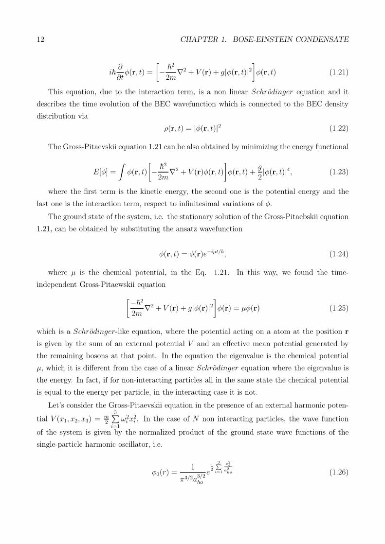
Figure 1.3: BEC density distribution for different values of positive scattering length (repulsiveinteraction). In the non interacting case the density distribution is a Gaussian (dotted line) whereas,by increasing the interaction it takes the form of an inverted parabola with a broadening which dependson the interactions strength. Adapted from [34]
with aho =√
~/mωho the harmonic oscillator length, and the BEC density distribution has
the form
n0(r) = N |φ0(r)|2. (1.27)
In the limit of strong interactions, i.e. Na ≫ aho, the interaction energy term in the time-
independent Gross-Pitaevskii equation is the dominant one and the kinetic energy term can be
neglected (Thomas− Fermi Approximation). In this situation, the equation takes the form
[
V (r) +4π~a
m|φ(r)|
]
φ(r) = µφ(r) (1.28)
and it can be analytically solved. In this situation the solution is
n0(r) =
1g[µ− V (r)] µ > V (r)
0 µ < V (r)(1.29)
which implies that for an harmonic potential the density distribution assumes the shape of
an inverted parabola

14 CHAPTER 1. BOSE-EINSTEIN CONDENSATE
n0(r) = −µ
g
(
1−3
∑
i=1
x2i
Ri
)
(1.30)
where Ri =√
2µmω2
iis the Thomas-Fermi radius in the ith direction.
In Fig.1.3 is shown how the repulsive interaction between atoms modifies the density dis-
tribution: it has not the form of the gaussian wavefunction of the harmonic oscillator ground
state anymore, as in the case of non interacting particles, but it is a broader inverted parabola
with a broadening depending on the interactions strength.
1.3 Feshbach resonances
How it has been introduced in the previous section, the effective interaction among the particles
in a dilute bosonic gas at low temperatures can be described in terms of a single parameter,
i.e. the scattering length a. This quantity can assume both positive and negative value and
the interaction between two particles is, respectively, attractive or repulsive. Anyway, there
is the possibility to change the scattering length value, and switching from a regime to an
other, by using Feshbach resonances. This property was studied for the first time in 1958 by
Feshbach in the field of nuclear physics [17], and it is important also in the field of cold atoms
[16, 35, 36]. In fact, thanks to the presence of these resonances, it is possible to tune the
interparticle interaction by simply changing a magnetic field acting on the atoms.
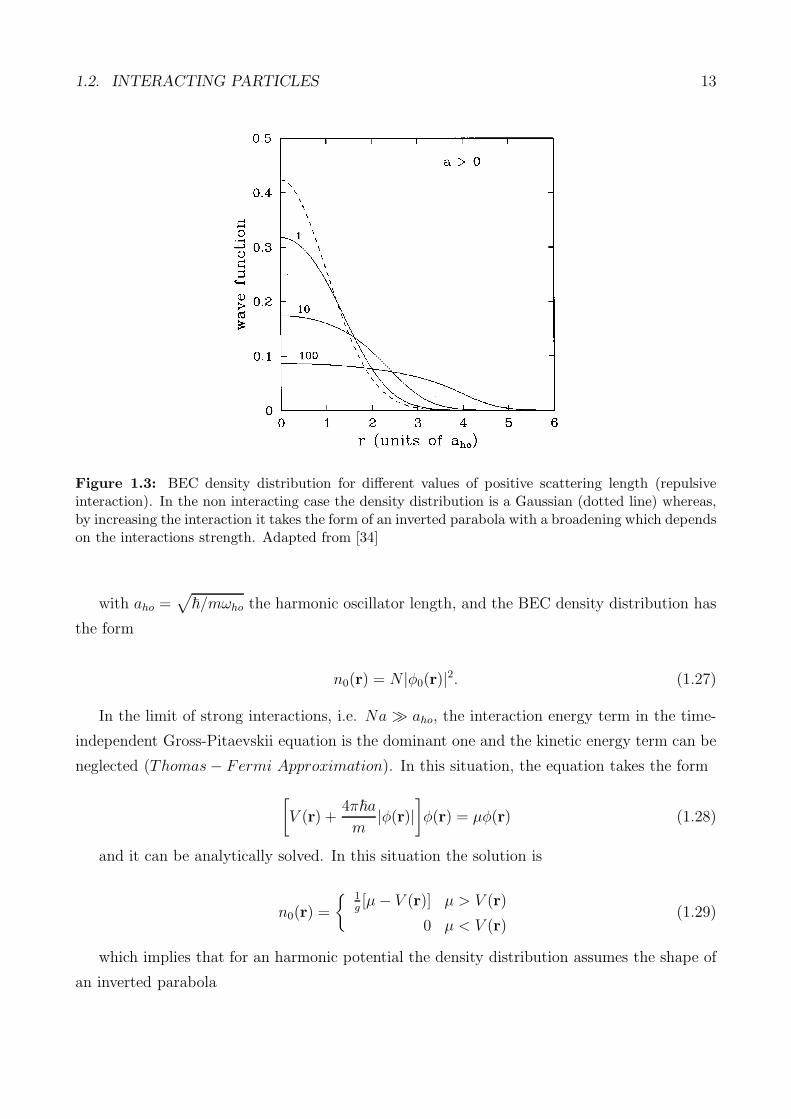
Let us talk about Feshbach resonances more in details and let us consider two diatomic
molecular potential curves, the ground state Vbg and the excited state Vexc, which correspond
to two different spin configurations4 (Fig.1.4). At large interparticle distances, i.e. for R → ∞,
the potential Vbg correspond to the energy of two free atoms and it is used as reference energy
(V∞ = 0). When two atoms collide, with a small energy E, the potential curve Vbg correspond
to the accessible channel for collisional processes and it is called “open channel”. The other
channel, which is known as “closed channel”, it is not accessible, but it may have a bound
molecular state close to 0. If the two atoms have the possibility to make a temporary transition
to this the bound state, then their scattering cross section can extremely increase.
Let us suppose that the magnetic moment of the atoms in the two channels is different.
In this case, it is possible to change the energy difference between the two states by simply
varying a magnetic field B thanks to the fact that the two potential curves have a different
4In general, a molecule has more than two potential curves, each of which corresponds to an hyperfine orZeeman level. For simplicity the description considers one excited state and it describes appropriately the caseof a single resonance.
1.3. FESHBACH RESONANCES 15
Figure 1.4: Model of the Feshbach resonance. The atoms in the open channel Vbg(R) collide with asmall energy E. If the collisional energy approaches the energy of the molecular bound state in theclosed channel Vext(R) (at the Feshbach resonance) the scattering cross section increases. By tuning amagnetic field, it is possible to the energy level of the closed channel, with respect to the open one.Adapted from [36]
response to the application of the field due to the Zeeman effect. In particular, by tuning the
magnetic field, it is possible to change the energy level of the closed channel, with respect to
the open one. At the (Feshbach) resonance, the energy of the two colliding atoms E approaches
the energy of the molecular bound state, by causing the increase of the scattering cross section.
The scattering length depends on the magnetic field B via
a(B) = abg
(
1− ∆
B − B0
)
(1.31)
where B0 is resonance center, ∆ the resonance width and abg the background scattering
length, i.e. the scattering length far from the resonance.
It is important to note that if the resonance is a general phenomenon, the parameters B0,
∆ and abg depend on the atomic species. Let us consider the specific case of the 39K,i.e.
the atom that we employ in the experiments. It has a background scattering length negative
(abg = −44a0, with a0 the Bohr radius), corresponding to an attractive interaction, which would
provoke the BEC collapse. However, it has also a wide Feshbach resonance and it is possible to
16 CHAPTER 1. BOSE-EINSTEIN CONDENSATE
340 360 380 400 420 440
-400
-200
0
200
400
B0
a (a
0)
B (G)
Bzc
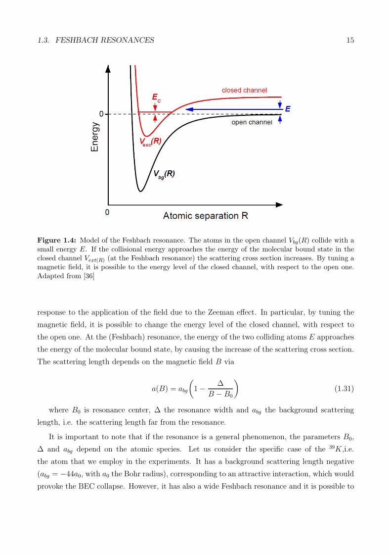
Figure 1.5: Scattering length a, in unit of Bohr radius, as a function of the magnetic field B for 39Katoms. The Feshbach resonance occurs at B0 ∼ 400G. Bzc and ∆ are zero-crossing magnetic field andthe resonance width respectively.
tune the value of the scattering length until it reaches positive value. Fig.1.5 shows a plot of
the scattering length a as a function of the magnetic field B of the 39K in the hyperfine state
|F = 1, mF = 1〉. In this situation B0 ≃ 402G and ∆ ≃ −52G. As it is shown in Fig 1.5, the
scattering length vanishes at a certain value of the magnetic field. It is known as zero-crossing
magnetic field Bzc = B0 +∆ and it is related to the scattering length via
a(B) =abg∆
(B − Bzc) (1.32)
if B → Bzc. It is important to note that by tuning the value ofabg∆
we control the interaction
around the vanishing interaction point. In particular, by decreasing the ratio we improve the
accuracy for tuning the interaction. In the case of 39K atoms, the sensitivity around Bzc = 350G
is da/dB ≃ 0.56a0/G and this implies that if the stability of the magnetic field is for example
1G, the interactions of the BEC can be nulled with an uncertainty of about half a Bohr radius.

1.4. OPTICAL DIPOLE POTENTIALS: RED DETUNED TRAP 17
1.4 Optical dipole potentials: red detuned trap
Another important feature of the Bose-Einstein condensates is the possibility to easily manip-
ulate and trap the atoms by using laser light. In order to understand how it is possible, let us
focus on the interaction between the atoms and a monochromatic electromagnetic radiation.
The presence of an electric field
E(r, t) = eE(r)e−iωt + h.c. (1.33)
induces on the atoms a dipole momentum, which oscillates at the same driving frequency ω
of the electric field E
p(r, t) = ep(r)e−iωt + h.c. (1.34)
Both in the electric field equation that in the dipole momentum one, e is the unit polarization
vector and E and p are, respectively, the amplitude of the electric field and of the dipole
momentum, which are related via p = αE, with α = α(ω) the complex polarizability.
Due to the interaction between E and p, a conservative dipole potential
Udip = −1
2〈pE〉 (1.35)
is present.
It is possible to demonstrate [37] that if the diving frequency ω is far from the atomic
resonance frequency ω0, which is the case of main practical interest, the dipole potential Udip
takes the simple form
Udip =3πc2
2ω30
(
Γ
∆
)
I(r) (1.36)
where ∆ = ω−ω0 is the detuning, whereas the scattering rate due to the far-detuned photon
absorption and subsequent spontaneous reemission by the atoms takes the form
Γsc =3πc2
2~ω30
(
Γ
∆
)2
I(r). (1.37)
In both cases I(r) = 2ǫ0c|E|2 is the field intensity. In order to reduce the value of the
scattering rate in the experiments, large detuning and high intensities are used, due to the fact
that Udip ∝(
Γ∆
)
, whereas Γsc =
(
Γ∆
)2
The detuning ∆ can assume both positive that negative value. In the first case, which is
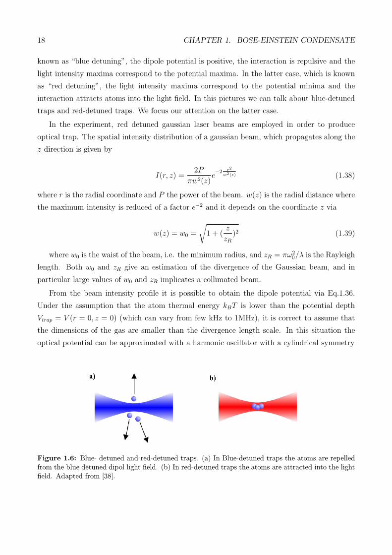
18 CHAPTER 1. BOSE-EINSTEIN CONDENSATE
known as “blue detuning”, the dipole potential is positive, the interaction is repulsive and the
light intensity maxima correspond to the potential maxima. In the latter case, which is known
as “red detuning”, the light intensity maxima correspond to the potential minima and the
interaction attracts atoms into the light field. In this pictures we can talk about blue-detuned
traps and red-detuned traps. We focus our attention on the latter case.
In the experiment, red detuned gaussian laser beams are employed in order to produce
optical trap. The spatial intensity distribution of a gaussian beam, which propagates along the
z direction is given by
I(r, z) =2P
πw2(z)e−2 r2
w2(z) (1.38)
where r is the radial coordinate and P the power of the beam. w(z) is the radial distance where
the maximum intensity is reduced of a factor e−2 and it depends on the coordinate z via
w(z) = w0 =
√
1 + (z
zR)2 (1.39)
where w0 is the waist of the beam, i.e. the minimum radius, and zR = πω20/λ is the Rayleigh
length. Both w0 and zR give an estimation of the divergence of the Gaussian beam, and in
particular large values of w0 and zR implicates a collimated beam.
From the beam intensity profile it is possible to obtain the dipole potential via Eq.1.36.
Under the assumption that the atom thermal energy kBT is lower than the potential depth
Vtrap = V (r = 0, z = 0) (which can vary from few kHz to 1MHz), it is correct to assume that
the dimensions of the gas are smaller than the divergence length scale. In this situation the
optical potential can be approximated with a harmonic oscillator with a cylindrical symmetry
Figure 1.6: Blue- detuned and red-detuned traps. (a) In Blue-detuned traps the atoms are repelledfrom the blue detuned dipol light field. (b) In red-detuned traps the atoms are attracted into the lightfield. Adapted from [38].

1.5. OPTICAL LATTICES 19
Vdip ≈ −Vtrap
[
1− 2
(
r
w0
)2
−(
z
zR
)2]
(1.40)
whose oscillation frequencies are
ωr =
(
4Vtrap
mw20
)1/2
(1.41)
and
ωz =
(
2Vtrap
mz2R
)1/2
. (1.42)
It is important to know that the Rayleigh length zR is πw0/λ larger than the minimum
waist w0 and consequently the force acting on the atoms along the longitudinal direction is
lower than that acting along the radial direction. This implies that it is essential to use more
than one single laser beam to tightly confine the atoms along all of the spatial directions.
1.5 Optical lattices
By using laser light it is possible to realize optical lattices, which are the perfectly periodic
potential for neutral atoms. As the optical trap, they can be employed to trap and to manipulate
the atoms.
Optical which are realized by superimposing two counter propagating laser beams. The
interference of the two laser beams produces a standing wave with a period equal to λ/2, where
it is possible to trap the atoms. In order to have a standing wave with a larger period, the angle
between the two beams must be smaller than 180. In the presence of Gaussian laser beams,
the potential trap is
V (r, z) ≈ −V0e−2r2/w2(z)sin2(kz) (1.43)
where k = 2π/λ is the lattice wave vector and V0 is the potential depth which can be written
in term of the recoil energy Er =~2k2
2mas
s =V0
Er
. (1.44)
It is important to note that if all of the parameters of the two laser beams are the same, V0 is four
times larger than Vtrap. This is the simplest case of 1D optical lattice, but it is also possible
to realize 2D or 3D optical lattices by superimposing, respectively, two or three orthogonal
standing waves, in order to avoid the interference term. In this situation, the potential depth
20 CHAPTER 1. BOSE-EINSTEIN CONDENSATE
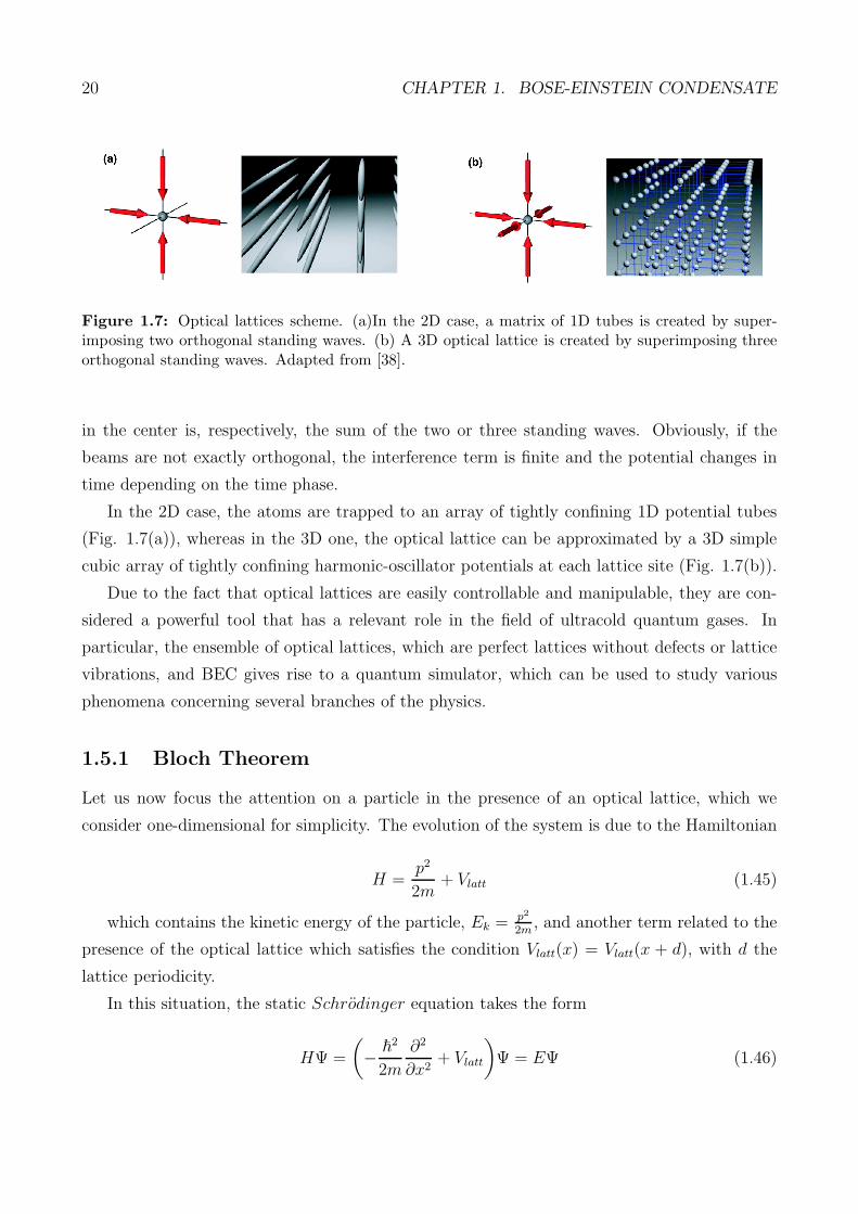
Figure 1.7: Optical lattices scheme. (a)In the 2D case, a matrix of 1D tubes is created by super-imposing two orthogonal standing waves. (b) A 3D optical lattice is created by superimposing threeorthogonal standing waves. Adapted from [38].
in the center is, respectively, the sum of the two or three standing waves. Obviously, if the
beams are not exactly orthogonal, the interference term is finite and the potential changes in
time depending on the time phase.
In the 2D case, the atoms are trapped to an array of tightly confining 1D potential tubes
(Fig. 1.7(a)), whereas in the 3D one, the optical lattice can be approximated by a 3D simple
cubic array of tightly confining harmonic-oscillator potentials at each lattice site (Fig. 1.7(b)).
Due to the fact that optical lattices are easily controllable and manipulable, they are con-
sidered a powerful tool that has a relevant role in the field of ultracold quantum gases. In
particular, the ensemble of optical lattices, which are perfect lattices without defects or lattice
vibrations, and BEC gives rise to a quantum simulator, which can be used to study various
phenomena concerning several branches of the physics.
1.5.1 Bloch Theorem
Let us now focus the attention on a particle in the presence of an optical lattice, which we
consider one-dimensional for simplicity. The evolution of the system is due to the Hamiltonian
H =p2
2m+ Vlatt (1.45)
which contains the kinetic energy of the particle, Ek =p2
2m, and another term related to the
presence of the optical lattice which satisfies the condition Vlatt(x) = Vlatt(x + d), with d the
lattice periodicity.
In this situation, the static Schrodinger equation takes the form
HΨ =
(
− ~2
2m
∂2
∂x2+ Vlatt
)
Ψ = EΨ (1.46)

1.5. OPTICAL LATTICES 21
whose solution, according to the Bloch theory [39], is a periodic plane wave,
Ψn,q = un,q(x)eiqx (1.47)
where the periodic term un,q(x) = un,q(x+ d) has the same lattice periodicity d.
As a consequence of the system periodicity, the eigenfunctions Ψn,q of the Schrodinger
equation and the eigenvalues En,q are characterized by two quantum numbers q and n. The
first one is called “quasi-momentum” and it is related to the translational symmetry of the
optical lattice.
It is important to note that the periodicity of the optical lattice is reflected also in the
reciprocal lattice, whose periodicity si G = 2π/d, and consequently
En,q(x) = En,q+G(x) (1.48)
Ψn,q(x) = Ψn,q+G(x) (1.49)
As a consequence of the reciprocal lattice periodicity, only the first Brillouin zone, i.e. the
elementary cell of the reciprocal lattice which ranges from q = −G/2 and q = G/2, is relevant.
The second quantum number, n, is called “band index”: for a given quasimomentum q, there
are several solution En(q) (which are continuous function of q) identified by the index n. This
solution are called “energy bands” and they are separated by forbidden zones, called energy
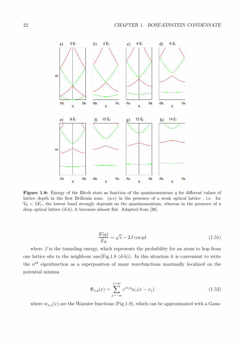
gaps. The energy bands behaves differently depending on the optical lattice depth. In the case
of weak optical lattice, i.e. s ≤ 5, the energy bands depends strongly on the quasimomentum
q and they take the form
E(q)
ER= q2 ∓
√
4q +s2
16(1.50)
where q = q/π/d − 1 and the minus sign is referred to the lower energy band whereas the
plus sign is referred to the first excited band. (Fig.1.8 (a-c) Under the assumption of weak
optical lattice, the only bound states belong to the first two energy band and this is due to
the fact that the gap energy between the nth band and the n + 1th ones scales as V n+10 . The
particles in the other excited state, instead, behaves as free particles. We observe the energy
gap at the end of the Brillouin zone, where q = π/d, and its value is ∆Egap =sER
2.
For deep optical lattices, i.e. for s ≥ 5, we are in the “tight-binding regime” and the energy
bands depend slightly on the quasimomentum as
22 CHAPTER 1. BOSE-EINSTEIN CONDENSATE
Figure 1.8: Energy of the Bloch state as function of the quasimomentum q for different values oflattice depth in the first Brillouin zone. (a-c) in the presence of a weak optical lattice , i.e. forV0 < 5Er, the lowest band strongly depends on the quasimomentum, whereas in the presence of adeep optical lattice (d-h), it becomes almost flat. Adapted from [38].
E(q)
ER
=√s− 2J cos qd (1.51)
where J is the tunneling energy, which represents the probability for an atom to hop from
one lattice site to the neighbour one(Fig.1.8 (d-h)). In this situation it is convenient to write
the nth eigenfunction as a superposition of many wavefunctions maximally localized on the
potential minima
Ψn,q(x) =
j=∞∑
j=−∞eixjqwn(x− xj) (1.52)
where wn,j(x) are the Wannier functions (Fig.1.9), which can be approximated with a Gaus-

1.5. OPTICAL LATTICES 23
Figure 1.9: Wannier functions (red) for two different values of lattice height s: (a) s = 3 and(b) s = 10. For s = 3 the sidelobes are visible, whereas in the other case they become very smallcorresponding to a tunneling probability decreases. Figure adapted from [38].
sian at the xthj lattice site.
1.5.2 Semi-Classical Dynamics
Let us now consider the dynamics of a particle subjected to an external force Fext. If the
external force varies slowly over the dimensions of the Bloch wave packet and it is weak enough
not to provoke interband transition, we can use the semiclassical model. From a classical point
of view, the behaviour of a particle subjected to an external force Fext, which is related to a
potential gradient, is set by the Hamilton equation
x =∂H
∂p(1.53)
p = −∂H
∂q. (1.54)
By assuming the analogy between the quasimomentum q and the momentum p, the semi-
classical equation of a wave packet in the first energy band can be written as
x = v(0) =1
~
dE
dq, (1.55)
i.e. the Bloch velocity vn(q) = 1h∂En(q)
∂qexpressed in terms of the average position of the
wave packet x, and
~q = −dV (x)
dx. (1.56)
24 CHAPTER 1. BOSE-EINSTEIN CONDENSATE
According to the semiclassical model, if the external force does not cause an interband
transition, it leaves the energy spectrum, due to the periodic potential, unchanged and only
the position and the quasimomentum of the particle are changed.
By comparing Eq.1.56, which is related to the particle acceleration, with the second Newton
law mx = −dV (x)/dx, it is possible to introduce a new mass,
1
m∗ =1
~2
d2
dq2E0
q . (1.57)
It is called the effective mass and it depends on the band curvature. Eventually, it may
become negative near the Brillouin zones boundaries, meaning that the external forces induce
the particle to accelerate in the opposite direction.
In the tight binding limit, by considering the behaviour of the energy spectrum in the Eq.
1.51, the effective mass has the form
m∗ = m
(
ER
J
)
1
π2 cos(qd)(1.58)
In particular, it depends on the energy band curvature and it tends to the real mass m in
the case of a free particle parabolic spectrum. The effective mass is an useful tool in order
to describe the dynamical behaviour of a particle in a periodic potential. The interest in this
concept is due to the fact that it is possible to use the classical mechanics to describe the
particle behaviour only if the mass of the particle is substituted with the effective mass which
takes into account the forces due to the presence of the periodic potential.
Chapter 2
Physics of 1D BEC
2.1 1D Quasi-condensate
As it was shown in Section 1.1, an important feature of one-dimensional systems is that in 1D
it is not possible to define a finite critical temperature Tc below which the ground state of the
system is macroscopically occupied and the transition to the BEC phase doesn’t occur [32].
In fact for one-dimensional systems the critical temperature for Bose-Einstein condensation is
the absolute zero, and so no BEC can exist at a finite temperature. Anyway, a degeneracy
temperature below which the quantum nature of particles cannot be ignored can be defined
and it takes the form
TD =~2
mkBn21D (2.1)
where n1D = N/L is the 1D density, with L the system length. Below this temperature, the
thermal De Broglie wavelength is comparable to the interparticle separation, the wavefunctions
of the particles are overlapped, but they do not share the same single-particle ground state.
For T < TD the system is in a new regime, i.e. the quasi-condensate one, which is characterized
by correlation properties different from those on 3D systems.
From a theoretical point of view, the correlation function between two wavefunctions sepa-
rated by at distance r is defined as
ρ(r) = 〈Ψ(r)†Ψ(0)〉 . (2.2)
For a pure 3D BEC with density of atoms in the ground state n0, the condition for Bose-
Einstein condensation is
25
26 CHAPTER 2. PHYSICS OF 1D BEC
lim|r|→∞
ρ(r) = n0 (2.3)
that is the correlation function is finite even at infinite distances. In fact the 3D BEC
is a macroscopic coherent object whose phase Φ(r) is well defined in the entire system. For
temperature above the critical temperature, the correlation function decays exponentially, as
in the classical systems. For a 1D system the situation is a bit different, due to the fact that
the strong phase fluctuations can destroy the long-range order of the system. As a matter of
fact, the mean square fluctuations of the phase for 1D systems are expected to linearly diverge
at large distances
lim|r|→∞
〈∆Φ(r)2〉 = lim|r|→∞
mkBT
n1D~2|r| → ∞, (2.4)
whereas the correlation function decays exponentially
ρ(r) ∝ n1De− |r|
2ξ (2.5)
where ξ is the correlation length
ξ =n1D~
2
mkB
1
T(2.6)
describing the distance over which the system is coherent. It is important to note that the
correlation length increases as the temperature decreases. As a consequence, lowering the
temperature, the gas behaves more and more like a true condensate. As it was introduced
above, in 1D there is no condensation due to the fact the correlation function approaches
zero at large distances. Anyway, if the correlation length is sufficiently large compared to the
system size L, i.e. ξ ≫ L, the phase coherence is preserved throughout the system, which thus
behaves as a real condensate. In the intermediate case, i.e. ξ > n1D, the correlation function
is zero only for some particles, depending on their mutual distance, whereas is finite for the
others. As a consequence, the gas is locally coherent and the correlation is broken on the full
length scale. This phase is called ”quasi-condensate” phase and the system has intermediate
properties between a real condensate and a normal system. In term of degeneracy temperature,
the condition required to observed a quasi condensate phase is
T
TD=
L/N
ξ< 1 (2.7)
In Fig. 2.1 the conditions for the different regimes are shown.
2.2. EXPERIMENTAL 1D SYSTEM 27
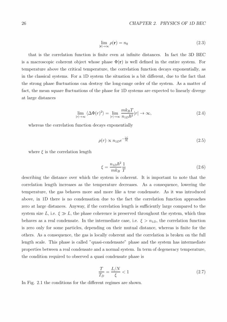
Figure 2.1: Different regimes of a 1D system of N bosons. For T > TD, ξ < L/N and the systemis the normal phase. For TD/N < T < TD, ξ > L/N and the system has intermediate propertiesbetween a real BEC and a normal system and it is in the “Quasi-Bec” phase. For T < TD/N thesystem is a real BEC. Figure adapted from [40].
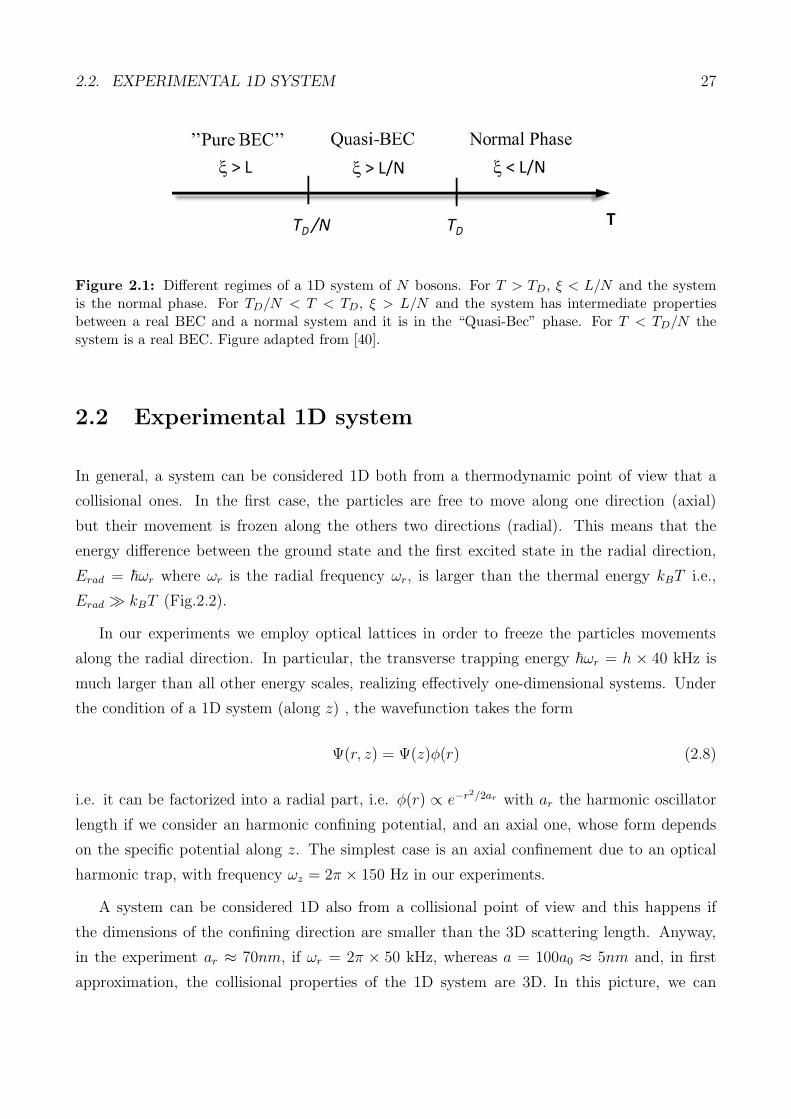
2.2 Experimental 1D system
In general, a system can be considered 1D both from a thermodynamic point of view that a
collisional ones. In the first case, the particles are free to move along one direction (axial)
but their movement is frozen along the others two directions (radial). This means that the
energy difference between the ground state and the first excited state in the radial direction,
Erad = ~ωr where ωr is the radial frequency ωr, is larger than the thermal energy kBT i.e.,
Erad ≫ kBT (Fig.2.2).
In our experiments we employ optical lattices in order to freeze the particles movements
along the radial direction. In particular, the transverse trapping energy ~ωr = h × 40 kHz is
much larger than all other energy scales, realizing effectively one-dimensional systems. Under
the condition of a 1D system (along z) , the wavefunction takes the form
Ψ(r, z) = Ψ(z)φ(r) (2.8)
i.e. it can be factorized into a radial part, i.e. φ(r) ∝ e−r2/2ar with ar the harmonic oscillator
length if we consider an harmonic confining potential, and an axial one, whose form depends
on the specific potential along z. The simplest case is an axial confinement due to an optical
harmonic trap, with frequency ωz = 2π × 150 Hz in our experiments.
A system can be considered 1D also from a collisional point of view and this happens if
the dimensions of the confining direction are smaller than the 3D scattering length. Anyway,
in the experiment ar ≈ 70nm, if ωr = 2π × 50 kHz, whereas a = 100a0 ≈ 5nm and, in first
approximation, the collisional properties of the 1D system are 3D. In this picture, we can
28 CHAPTER 2. PHYSICS OF 1D BEC
Figure 2.2: In 1D the particles are free to move along one direction (axial) but their movement isfrozen along the others two directions (radial). Due to the strong transverse harmonic confinement,i.e. ~ωr is larger than all other energy scales, only the radial ground state is occupied. In the axialdirection, also the excited states can be occupied. Occupied levels are represented in red, empty levelsin gray. [40]
introduce a new coupling constant
g1D =2~
m
a
a2r=
2~
ma1D(2.9)
with a1D = a2rais the 1D scattering length under the condition ar ≫ a. If this condition is
not satisfy, as near the Feshbach resonance, the 1D scattering length takes the form
a1D =a2r2a
(
a− Ca
ar
)
(2.10)
with C = 1.0326 [41]. This formula works for any value of a/ar.
2.3 Momentum distribution and correlation
In our experimental system, the experimental observable employed to study the correlation
properties of our system is the momentum distribution ρ(p), which is related to the spatially
2.3. MOMENTUM DISTRIBUTION AND CORRELATION 29
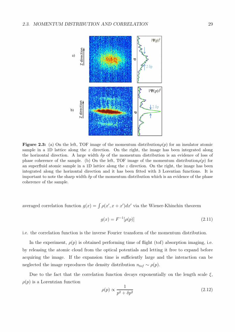
Figure 2.3: (a) On the left, TOF image of the momentum distributionρ(p) for an insulator atomicsample in a 1D lattice along the z direction. On the right, the image has been integrated alongthe horizontal direction. A large width δp of the momentum distribution is an evidence of loss ofphase coherence of the sample. (b) On the left, TOF image of the momentum distributionρ(p) foran superfluid atomic sample in a 1D lattice along the z direction. On the right, the image has beenintegrated along the horizontal direction and it has been fitted with 3 Lorentian functions. It isimportant to note the sharp width δp of the momentum distribution which is an evidence of the phasecoherence of the sample.
averaged correlation function g(x) =∫
ρ(x′, x+ x′)dx′ via the Wiener-Khinchin theorem
g(x) = F−1[ρ(p)] (2.11)
i.e. the correlation function is the inverse Fourier transform of the momentum distribution.
In the experiment, ρ(p) is obtained performing time of flight (tof) absorption imaging, i.e.
by releasing the atomic cloud from the optical potentials and letting it free to expand before
acquiring the image. If the expansion time is sufficiently large and the interaction can be
neglected the image reproduces the density distribution ntof ∼ ρ(p).
Due to the fact that the correlation function decays exponentially on the length scale ξ,
ρ(p) is a Lorentzian function
ρ(p) ∝ 1
p2 + δp2(2.12)
30 CHAPTER 2. PHYSICS OF 1D BEC
whose half width at half maximum δp is related to ξ via
δp =0.63~
ξ(2.13)
The behaviour of δp gives information related to the system nature. A large width of
the momentum distribution is an evidence of loss of phase coherence of the sample. In this
situation the correlation function decays on a length scale ξ lower than the lattice spacing d.
Consequently when the system is in an insulating phase, we observe a large δp (Fig.2.3a). If
the system is in the superfluid phase, the momentum distribution has a sharp δp (Fig.2.3b),
which is an useful tool to obtain information about the temperature of the sample. In fact, as
the coherence length ξ, also the momentum distribution δp depends on temperature, and, in
particular, an increase of the temperature provokes an increase of δp.
2.4 Theoretical model for 1D systems
2.4.1 Luttinger Liquid
One-dimensional interacting fluids, both bosonic and fermionic, obey a new paradigm, i.e. the
“Luttinger liquid” one [42]. This kind of systems are characterized by low energy excitations,
which are collective modes with a linear dispersion relation. A simple explanation of the
collective behaviour is the following: due to the interactions among the particles and the strong
confinement in the radial direction, if a particle moves in the only allowed direction, it pushes
the neighbour one, which in turn moves the next one and so on, turning into a collective
motion the movement of a individual particle. Thanks to the presence of this collective modes,
it is possible to use the bosonization technique [43, 44], which is efficient both for bosons and
fermions, to study the one-dimensional systems. In this construction, the one-dimensional fluids
are described in terms of a field operator Φl(z) which is a continuous function of the position z.
In 1D, due to the fact that there is a unique way to enumerate the particles by starting from
z = −∞ and proceeding to the right direction, the field operator Φl(z) labelling the particles,
can be always taken as an increasing function of z, differently from the 3D case. In the case of
bosons, a suitable definition of the field operator is [43]
Φl(z) = 2πn1Dz − 2φ(z) (2.14)
where n1D = N/L is the mean density of the system and φ(z) is a slowly varying quantum
field. In terms of this field, the density operator ρ(z) takes the form

2.4. THEORETICAL MODEL FOR 1D SYSTEMS 31
ρ(z) = (n1D − 1
π∂zφ(z))
∑
m
αme2im(πn1Dz−φ(z)) (2.15)
where m is an integer number and αm is a non-universal coefficient which depends on the
system details. In this situation, the single particle creation operator Ψ†(z) can be written as
Ψ†(z) =√
ρ(z)e−iθ(z) (2.16)
where θ(z) is an operator which depends on the system details. In the case of a BEC, it is
the superfluid phase. In general, the evolution of a system of N interacting boson in an optical
lattice Vlatt(r), subjected to an external potential Vext(r) is driven by the Hamiltonian H , which
in second quantization takes the form
H =
∫
drΨ†(−~
2
2m∇2 + Vext(r) + Vlatt(r)
)
Ψ +g
2
∫
drΨ†Ψ†ΨΨ (2.17)
A representation of the Hamiltonian for the 1D interacting bosons, can be obtained by
putting the field operator 2.16 into the Hamiltonian 2.17. Under the assumptions that Vext(r) =
Vlatt(r) = 0, it takes the form of a quadratic Hamiltonian
HLL =~
2π
∫
dz[vsK(∂z θ(z))2 +
vsK
(∂zφ(z))2] (2.18)
where vs and K are the “Luttinger parameters”. The two parameters are linked to each
other via
vsK =π~n1D
m(2.19)
vsK
=Eint
π~(2.20)
where Eint is the interparticle interaction energy. Both parameters characterized entirely a
1D system in the regime of low energy and far from the Mott insulator transition (if a lattice
is present). In particular vs is the sound velocity of the system excitations which are sound-
like density-waves with a linear dispersion relation ω ∼ vk, whereas the parameter K is an
adimensional quantity, related to correlation at long distances, whose value is between 1 and
∞. If K = ∞ the bosons are non interacting. On the contrary, if 0 < K < ∞, the boson
are interacting and the correlation function decays as the Luttinger parameter K increases as
(2K)−1. In the case of K = 1 the system is strongly interacting and it behaves as spinless
fermions (Tonks-Girardeau gas [45]): in order to minimize their mutual repulsion, the particles
32 CHAPTER 2. PHYSICS OF 1D BEC
tend to occupy a fixed position and the wavefunctions of the particles cannot overlap. This
behaviour is similar to the fermions one which cannot stay in the same place in order to satisfy
the Pauli exclusion principle. Obviously, the particles are bosons, and the system wavefunction
is always symmetric under the exchange of two particles. The case of negative K is reached in
the presence of long range interactions.
2.4.2 Lieb-Liniger Model
As we have shown in section 1.2, in the presence of a system of N interacting bosons strongly
confined in the radial directions, only the binary collisions among the particles play a relevant
role which can be written in terms of the contact pseudopotential
Vcon = g1Dδ(zi − zj) (2.21)
where g1D is the one-dimensional constant coupling (Eq. 2.9). In this scenario, under
the assumption that the external potential Vext(z) = 0 , the Hamiltonian driving the system
evolution takes the form
H =
N∑
i=1
− ~
2m
∂2
∂z2i+ g
N∑
i<j=1
δ(zi − zj) (2.22)
This model, introduced by Lieb and Liniger in 1963 [46, 47], is the simplest non-trivial
model of interacting bosons in the continuum and it can be solved by using the using the
Bethe ansatz. It is useful to describe the system by using an adimensional parameter, known
as “Lieb-Liniger parameter”
γ =mg1D~2n1D
, (2.23)
which represents the ratio between the interaction energy, Eint ≈ g1Dn1D, and the kinetic
energy required to take a particle at a distance d = n−11D, Ecin ≈ ~
2n21D/m. It is important
to note that the Lieb-Liniger parameter increases as the mean density decreases. Therefore,
in one-dimension, the interaction energy increases with respect to the kinetic energy when the
density decreases, unlike that in three dimension. The Luttinger parameters which have been
introduced in the previous section, can be written in term of the Lieb-Liniger parameter. In
particular if γ ≪ 1
vs = vF
√γ
π
(
1−√γ
2π
)1/2
(2.24)
2.4. THEORETICAL MODEL FOR 1D SYSTEMS 33
K =π√γ
(
1−√γ
2π
)−1/2
(2.25)
and the system is in the bosonic limit, whereas if γ ≫ 1 (in the presence of low density or
strong interaction)
vs = vF
(
1− 4
γ
)
(2.26)
K =
(
1 +4
γ
)
. (2.27)
and the system is a Tonks-Girardeau gas.
2.4.3 Bose-Hubbard Model
In order to describe the system of N interacting boson in a deep optical lattices Vlatt(r) (s > 5)
subjected to an external potential Vext(r) , it is useful to use the Bose-Hubbard model.
The system evolution is driven by the Hamiltonian H , which in second quantization takes
the form
H =
∫
drΨ†(−~
2
2m∇2 + Vext(r) + Vlatt(r)
)
Ψ +g
2
∫
drΨ†Ψ†ΨΨ (2.28)
In the tight binding regime, the field operator Ψ can be written as a combination of Wannier
functions of the lowest Bloch energy band
Ψ(r) ≈∑
i
wi(r)bi, (2.29)
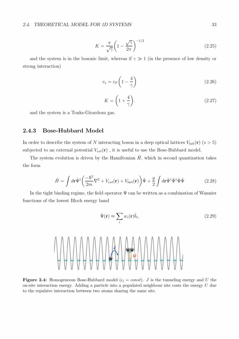
Figure 2.4: Homogeneous Bose-Hubbard model (ǫi = const). J is the tunneling energy and U theon-site interaction energy. Adding a particle into a populated neighbour site costs the energy U dueto the repulsive interaction between two atoms sharing the same site.
34 CHAPTER 2. PHYSICS OF 1D BEC
where bi is the annihilation operator of the ith site, and the Hamiltonian takes the form
H = −J∑
i
(b†i bi+1 + h.c) +U
2
∑
i
ni(ni − 1) +∑
i
(ǫi − µ)ni (2.30)
where bi is the creation operator of the ith site, ni = b†i bi is the number operator related
to the site occupancy and µ is the chemical potential. This Hamiltonian is known as Bose-
Hubbard Hamiltonian
Let’s focus the attention on the single terms of the Hamiltonian (Fig.2.4). The first one is the
kinetic energy of the system, which is proportional to the tunneling energy
J = −∫
drw ∗ (r− ri)
[−~2
2m∇2 + Vlatt(r)
]
w(r− ri+1) (2.31)
The tunneling energy J is related to the superposition of the Wannier functions localized
to the ith and the (i + 1)th sites, and it represents the probability for an atom to hop from
one lattice site to another. By estimating the tunnelling energy via Eq.2.31, once the Wannier
functions are known, it is possible to find a relation between the tunneling energy J in the
lattice and the parameter s, i.e.
J
Er= 1.43s0.98e−2.07
√s (2.32)
which implies that by tuning the intensity of the laser employed to realize the lattice it is
possible to change the tunneling energy. The second term of the Hamiltonian is proportional
to the interaction energy
U = g
∫
dr|w(r)|4. (2.33)
which quantifies the energy cost to put two particle in the same lattice site. It depends on the
coupling parameter g, which must be substituted by g1D in the presence of 1D lattice, and it
can be tuned by using the Feshbach resonance. Note that this is the only term which takes
into account the interaction among particles: interactions among atoms in different sites are
neglected. The last term takes into account the presence of an external potential. In fact, in
the experiment with ultracold quantum gases an external trap potential is usually present and
it provokes an energy offset ǫi in the ith site. If we have an harmonic trap, the energy offset is
ǫi =α
2
∑
i
(i− i0)2 (2.34)
where α is the harmonic trap strength and i0 is the trap center. If one assumes that the trap
2.4. THEORETICAL MODEL FOR 1D SYSTEMS 35
potential varies smoothly across the lattice, ǫi can be considered as a constant.
2.4.4 Superfluid and Mott Insulator
Let’s consider the Bose Hubbard Hamiltonian, by neglecting the last term due to the presence
of an external potential. In this situation the two relevant energy scale are the tunneling energy
J and the interaction one U . Depending on the interaction among particles, the system can
undergo a phase transition from a conductive phase to an insulator one induced by interac-
tions, which suppress the tunneling from site to site. In order to treat this phenomenon more
in detail, let’s consider the two different cases, U ≪ J and U ≫ J .
If the interaction among the particles is negligible compared to the tunneling energy, U ≪ J ,
all of the particles are free to move across the lattice and they occupy the Bloch ground state.
In this situation, they are delocalized throughout the lattice and the system is said to be in
a superfluid phase. By assuming that the Bloch ground energy state of a single delocalized
particle is a superposition of the wavefunctions localized on each lattice site,∑
i b†i |0〉, the
system ground state of N identical bosons is the product of N identical Bloch waves
|ΨSF 〉 ∝(
∑
i
b†i
)N
|0〉 . (2.35)
In this regime, in agreement with the Heisenberg uncertainty principle, the number of
particles per site is not determined but it follows a Poissonian distribution, while for each
site the phase is perfectly defined, giving rise to narrow peaks in the multiple matter wave
interference. If the interactions among the particles are strong enough to overcome the kinetic
energy, U ≫ J , for the bosons it is energetically convenient to stay apart and localize at each
lattice site, instead of flowing through the lattice. In fact an atom jumping from a site to a
neighbour one would cause an energy cost for the system equal to U . As a consequence, the
system is in an insulating phase, the Mott insulator, whose ground state is given by the product
of the single-site Fock states
|ΨMI〉 ∝∏
i
(b†i )N |0〉 . (2.36)
In this situation, the particle number per site is perfectly determined, but there is no
phase correlation between wavefunction localized at each site. As a result, no macroscopic
phase coherence holds. In order to have a pure Mott insulator, each lattice site must to be
occupied by an integer number of atoms. On the contrary, the superfluid phase coexists with

36 CHAPTER 2. PHYSICS OF 1D BEC
the insulating one.
The value at which the quantum transition from the superfluid phase to the insulating one
occurs, i.e. (J/U)c, depends on the chemical potential µ and on the site filling n as it shown in
Fig. 2.5.
Figure 2.5: Phase diagram of the SF to MI transition in a homogeneous case as a function of µand J , both normalized to U . The MI zones are characterized by an integer number of particles foreach lattice site, whereas in the superfluid phase it is possible to introduce only a mean filling. Notethat a larger average occupancy n implies a larger interaction energy to enter in the Mott phase andconsequently a smaller critical value (J/U)c. Red line: The decrease of the chemical potential µ/U atconstant J/U along the trap implies a succession of MI zones and SF ones. Adapted from [38].
In the MI phase the site filling is well defined and it is an integer number, whereas in the
superfluid phase only an average filling can be introduced, due to the fact that the number of
particles for each lattice site is not determined. Note that a larger average occupancy n implies
a larger interaction energy to enter in the Mott phase and consequently a smaller critical value
(J/U)c.
So far we have considered the homogeneous case. Anyway, in the experiments, it is difficult to
have an homogeneous system, due to the presence of an external trapping potential. In fact, if
the trap potential does not varies smoothly across the lattice, the last term in the BH hamil-
tonian cannot be neglected anymore, and the system has some regions with a commensurate
filling and some with an incommensurate one. In this situation, the system can be thought to
2.4. THEORETICAL MODEL FOR 1D SYSTEMS 37
be characterized by a local chemical potential which slowly varies from site to site and reaches
its maximum at the center of the harmonic potential. The variation of the chemical potential
provokes a change also in the local filling and in particular an increase of µ implies an increase
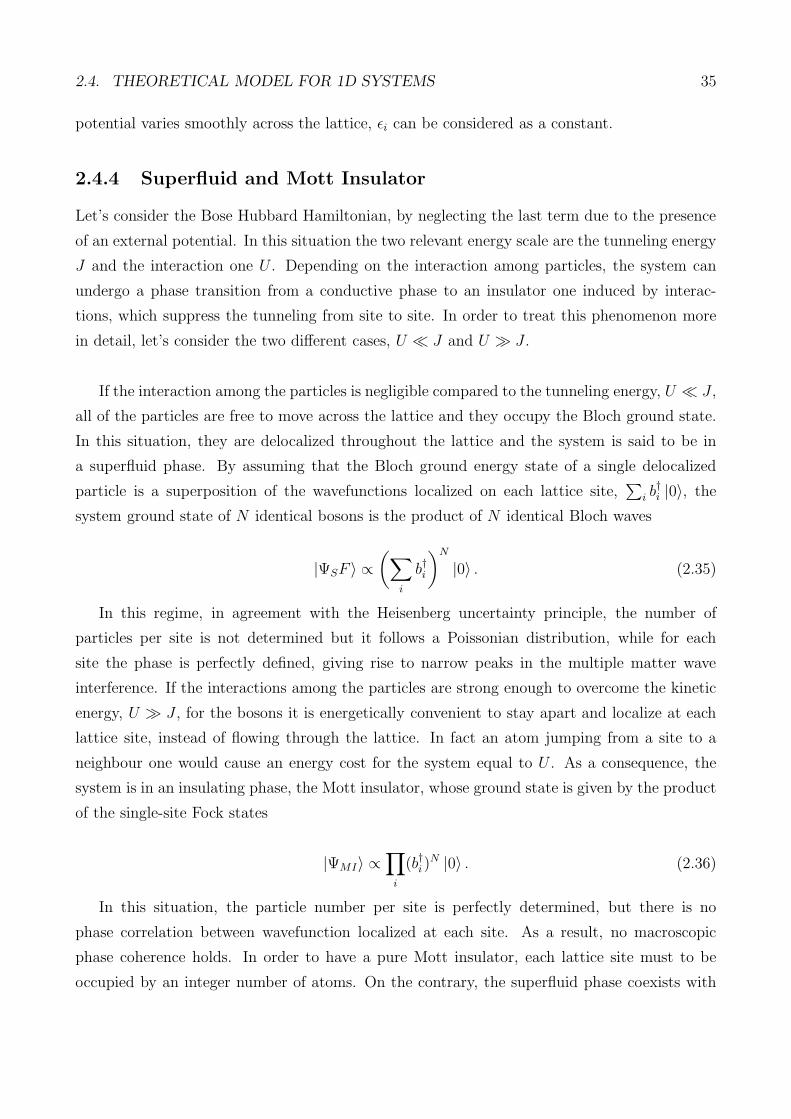
of the local filling. For a given value J/U < (J/U)c, the atoms alternate different phases de-
pending on their position across the lattice and we observe a shell structure where shells of the
Mott insulator are interchanged by shells of superfluid (Fig.2.6). In the limit case of J = 0,
only the MI phase survives and the density profile of the trapped atoms shows the so called
wedding-cake shape: all sites are filled with an integer number of particles and the central sites
have the largest filling.
Figure 2.6: In an inhomogeneous system, for a given value J/U < (J/U)c, the atoms alternatedifferent phases depending on their position across the lattice and we observe a shell structure whereshells of the Mott insulator are interchanged by shells of superfluid [38]
The Mott insulator phase was observed for the first time in an atomic systems in 2002
by Greiner et al.[24]. They increased the ratio U/J by increasing the lattice height s and
they observed a loss of phase coherence in the momentum distribution, which confirmed the
transition from a superfluid phase to an insulating one (Fig.2.7).
In the same experiments, they also verify the presence of the Mott insulator by probing the

38 CHAPTER 2. PHYSICS OF 1D BEC
Figure 2.7: Momentum distribution for different values of 3D lattice height s. By increasing s (from(a) to (h)) the system undergoes a phase transition from the superfluid coherent phase to the Mottinsulator incoherent phase. Adapted from [38].
excitation spectrum. The superfluid phase and the insulating one, in fact, are characterized
by a different spectrum, which are related to their different conductivity properties. When the
system is in the superfluid phase, due to gapless energy spectrum, any amount of energy can
be transferred in the system and the atoms are able to move from one lattice site to another
one. Conversely, in the MI phase the atoms are not free to move due to discontinuous energy
spectrum with a gap of the order of on site interaction energy U . A simple explanation for the
origin of this gap is the following. The lowest lying excitation in a system with an atom in each
lattice site is the creation of a particle-hole pair, where an atom in a lattice site is added into
a neighbour one holding an other atom. The energy of this configuration, where two atoms
are in the same lattice site, is raised by an amount U in energy above the configuration with a
single atom in each lattice site, due to the on-site interaction energy U 1. Consequently, in an
homogeneous system, removing an atom from a site and adding it to a neighbouring one with
the same occupancy has an energy cost equal to the on-site interaction energy U . Anyway, as it
was introduced above, we may have an inhomogeneous system which has different lattice sites
with different occupancy. In this situation it is possible to add an atom to a neighbouring site
with different occupancy by paying an energy cost equal to 2U .
1This explanation is valid also if the number of atoms in each lattice site is n
2.5. SINE-GORDON MODEL 39
2.5 Sine-Gordon Model
In the case of a weak optical lattice, the system dynamics is well described by the Sine-Gordon
model, which consider the optical potential Vlatt(z) = V0 cos(Gz) as a perturbation [44]. The
total Hamiltonian driving the system evolution can be obtained by starting from the general
Hamiltonian (Eq.2.17) where a perturbation potential is added and where the expression in eq.
2.15 is used for the density. In this situation, the Sine-Gordon Hamiltonian takes the form
HsG = HLL +g1Dπ
∫
dxcos(2pφ(x) + δx) (2.37)
where δ = nG−2pπn1D measures the system degree of incommensurability and in particular
δ = 0 corresponds to a commensurate number of bosons for each lattice. In the δ, p is an integer
number and the case p = 1 correspond to an integer number of bosons for each lattice site,
whereas higher values of p correspond to a one boson every p lattice sites. In the presence of
an integer filling, it is possible to recover the quantum transition from the superfluid phase
to the Mott insulator one also by starting from the Sine-Gordon Hamiltonian. By using the
renormalization group (RG) approach on the Sine-Gordon Hamiltonian, we find that the phase
transition occurs at a universal value of the Luttinger parameter Kc = 2/p2: for K > Kc the
system is in a superfluid phase and the optical lattice behaves as a negligible perturbation,
whereas in the opposite case the system is in the Mott insulating phase.

40 CHAPTER 2. PHYSICS OF 1D BEC

Chapter 3
Phase Slips in one dimensional systems
3.1 Phase slips in superconductors
The intriguing phenomenon of superconductivity was observed for the first time by the dutch
physicist Heike Kamerlingh Onnes in 1911 [48]. By studying the behaviour of the resistance
of solid mercury at cryogenic temperatures, he found that below a critical temperature TC ,
the resistance of mercury abruptly disappeared. In subsequent decades, the phenomenon of
superconductivity was observed in several other materials and, since its discovery, it has been
widely studied both from a theoretical point of view and an experimental one. Thanks to the
advent of modern technology, such as lithographic techniques and thin film deposition, it has
been possible to realize new experimental systems and answer to new theoretical questions. One
of these questions is if it is possible to observe the phenomenon of superconductivity in one-
dimensional (1D) systems. Obviously, the answer to this question has important implications
both in fundamental physics and practical applications. From a theoretical point of view, in
a 1D system it is not possible to observe the phenomenon of superconductivity, due to the
presence of thermally activated phase slips (TAPS) [1], which give rise to a finite resistance
also for temperatures below TC .
The first theoretical proposal for TAPS was made by Little in 1967 to understand the
mechanism of the supercurrent decay in a ring made of a thin wire [1]. His starting point was
that strong enough thermal fluctuations can provoke deviations from their equilibrium values of
both modulus and phase of the complex order parameter |Ψ(x)|eiφ(x) describing the superfluid
state (Fig. 3.1a). Due to thermal fluctuation, the modulus of the order parameter in a point of
the wire is suppressed and at the same time a 2πn phase jump is observed, with n an integer
number (Fig. 3.1 b). After the formation of phase slips, the modulus returns to its initial value
and the system gets back to its initial state with an accumulated phase shift of 2πn (Fig.3.1c).
41

42 CHAPTER 3. PHASE SLIPS IN ONE DIMENSIONAL SYSTEMS
Due to the rareness of the phase slip events, it is possible to consider only the cases n = ±1.
Figure 3.1: Cartoon of a phase slip event. (a) Before a phase slip event, the complex order parameter|Ψ(x)|eiφ(x) is characterized by a modulus |Ψ(x)| (dotted blue line) and a phase φ(x) (solid red line).(b) During a phase slip event, the modulus of the order parameter is suppressed and the phase makesa 2π phase jump. (c) After a phase slips event, the modulus is restored but both the phase gradientand the velocity v(x) are reduced. Adapted from [49].
Following a phase slip event, a finite voltage V appears across the wire due to the Josephson
relation between V and φ, i.e. V = ~φ2e . If there is not a bias current, there are the same
numbers of positive (n = 1) and negative (n = −1) phase slips and consequently the net voltage
is zero. Instead, in the presence of a bias current I ∝ |Ψ(x)|∇φ, the system is more inclined
to create positive phase slips, since the work performed by the current is positive for positive
phase slips, and the system is subject to a finite voltage and, at the same time, to a finite
resistance R = V/I.
The first quantitative theoretical model to estimate the resistance was developed by Langer
and Ambegaokar [2] and it was modified by McCumber and Halperin [3], few years later. Their
model was based on the idea that phase slips occur when the order parameter passes, via
thermal activation, over the free energy barrier ∆F separating states whose value of ∆φ differ
by 2π. They estimated the free energy barrier height by using the mean-field Ginzburg-Landau
equation, and they found that in a narrow superconducting channel, the free energy barrier
depends on the condensation energy density Hc and on the volume Aξ(T ), where A is the wire’s
cross section area and ξ(T ) the Ginzburg-Landau coherence length, via
∆F =8√2
3
Hc(T )2
8π(Aξ(T )) (3.1)
The rate of thermal activated phase slips is given by an Arrhenius type equation via
Ω(T )e−∆F/kBT where
Ω(T ) = (L
ξ(T ))(∆F
kBT)1/2(τGL)
−1 (3.2)

3.1. PHASE SLIPS IN SUPERCONDUCTORS 43
is the attempt frequency. Here L is the wire’s length and τGL = π~8kB(Tc−T )
is the relaxation
time of the time-dependent Gitzburg-Landau theory. By considering a narrow superconducting
channels with a finite current I, the voltage due to the presence of TAPS is
V =~Ω(T )
ee− ∆F
kBT sinh(I
I0) (3.3)
where I0 = 4ekBT/h. In the limit of low current, i.e. I ≪ I0, the resistance is
RLAMH = V/I ≃ Rq
(
~Ω(T )
kBT
)
e− ∆F
kBT (3.4)
where Rq =h
(2e)2.
The first measurement of a finite voltage for temperatures lower than TC was performed
by Lukens et al. [50] in 1970 by studying the voltage behaviour as a function of the current
in a one dimensional single-crystal tin whiskers (Fig. 3.2). They found that the voltage as a
function of the current near the transition behaved consistently with the Langer-Ambegaokar
model, i.e. V ∝ sinh(I/I0), confirming the presence of thermally activated phase slips.
As the temperature decreases, due to the increase of the height of the free energy barrier
∆F , the probability of TAPS becomes very small and phase slips cannot occur due to thermal
activation. Anyway, it has been suggested that at very low temperatures, phase slips should
be induced by quantum fluctuation of the order parameter [51, 52]. The first heuristic model
for quantum phase slips (QPS) in thin superconducting wires was proposed by Giordano [4] in
1988, in order to explain the discrepancy between the measured resistance of a narrow In strip
as a function of the temperature and the LAMH model, in the case of very low temperature
(Fig. 3.3).
He started by considering the motion of a damped particle moving in a tilted washboard
potential and assuming that it can be considered as a harmonic oscillator in a well, with a
natural frequency ω0. In this situation, the tunneling rate has the form
ΓMQT = B
√
V0ω0
~e
−aV0~ω0 (3.5)
where a and B are constant and V0 is the barrier height which coincides with the free energy
barrier ∆F in the case of a thin superconducting wires. Since the natural frequency ω0 can be
identified with the inverse of the Gitzburg-Landau relaxation time τGL, the tunneling rate has
the form
ΓMQT = B
√
∆F
~τGLe
−a∆FτGL~ (3.6)
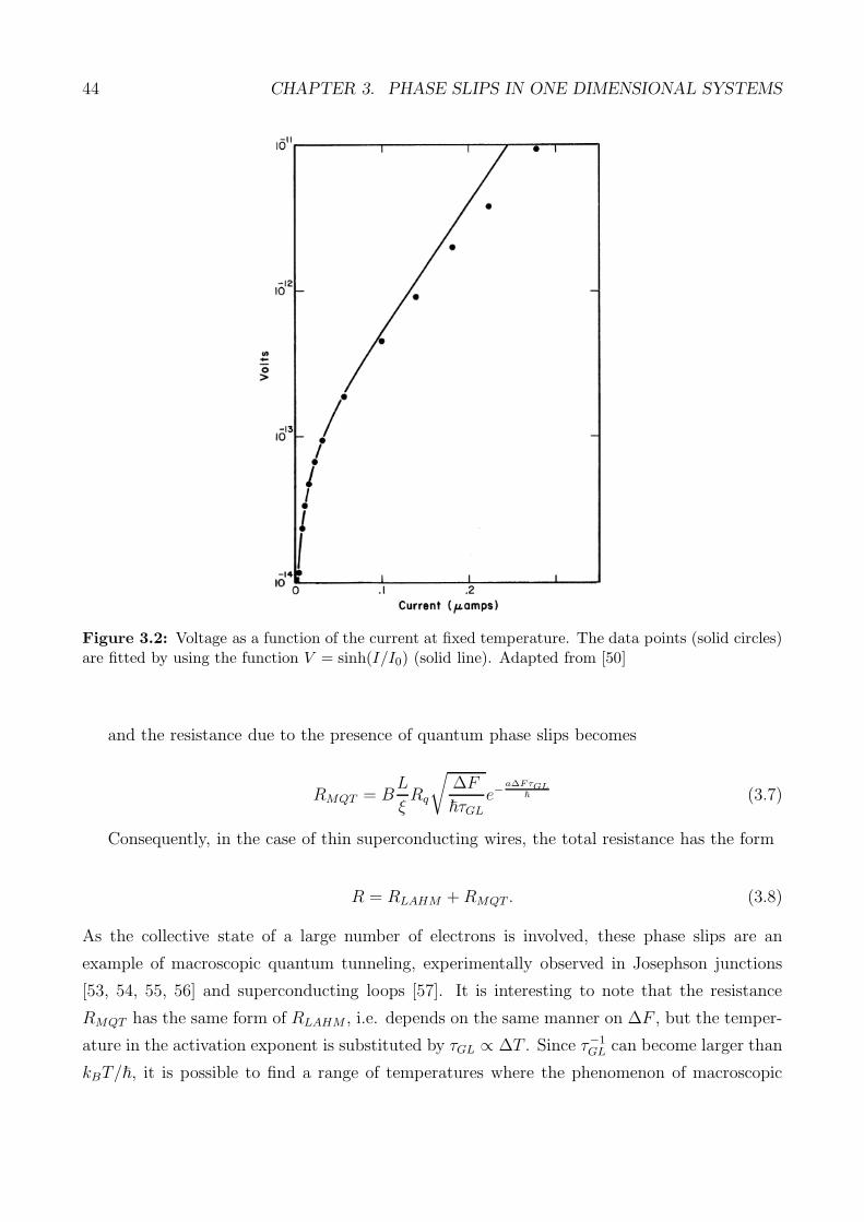
44 CHAPTER 3. PHASE SLIPS IN ONE DIMENSIONAL SYSTEMS
Figure 3.2: Voltage as a function of the current at fixed temperature. The data points (solid circles)are fitted by using the function V = sinh(I/I0) (solid line). Adapted from [50]
and the resistance due to the presence of quantum phase slips becomes
RMQT = BL
ξRq
√
∆F
~τGLe−
a∆FτGL~ (3.7)
Consequently, in the case of thin superconducting wires, the total resistance has the form
R = RLAHM +RMQT . (3.8)
As the collective state of a large number of electrons is involved, these phase slips are an
example of macroscopic quantum tunneling, experimentally observed in Josephson junctions
[53, 54, 55, 56] and superconducting loops [57]. It is interesting to note that the resistance
RMQT has the same form of RLAHM , i.e. depends on the same manner on ∆F , but the temper-
ature in the activation exponent is substituted by τGL ∝ ∆T . Since τ−1GL can become larger than
kBT/~, it is possible to find a range of temperatures where the phenomenon of macroscopic

3.1. PHASE SLIPS IN SUPERCONDUCTORS 45
Figure 3.3: Resistance, normalized by the normal state value, as a function of the temperature, forthree different values of the sample diameters. The solid curves are fits realized by using Eq. 3.4 whichconsider the presence of thermally activated phase slips , whereas the dotted curves are fits realizedby using Eq.3.8 which consider also the presence of quantum phase slips. Adapted from [4]
quantum tunneling dominates on the thermal activation of phase slips.
Since their first observation, phase slips (both thermal and quantum) have been the objects
of interest by the scientific community. They have been studied in different condensed-matter
systems, such as superconducting nanowires [58, 59, 11, 60, 61, 62] and Josephson junction
arrays [15], where the phase-slip nucleation rate is controlled by tuning the temperature or the
current. The phase-slip phenomenon is interesting not only from a theoretical point of view but
also from an experimental one. Since the last few years, theoretical proposal of devices based on
the phenomenon of quantum phase slips have been made and it would be interesting to realize
them experimentally. For example, it would be interesting to realize the quantum phase slip
junction [63], or the superconducting phase slips oscillator [64] or topologically-protected qubits
[63, 65] or a quantum standard for the electrical current [15]. These are just a few examples
of possible applications of the phase slips. Additional applications will certainly be possible in
the future, but a greater understanding of the phenomenon is needed in order to realize devices
based on phase slips. Thanks to the easy control and manipulation of their key properties, the
ultracold quantum gases are a good candidate to better understand this phenomenon.

46 CHAPTER 3. PHASE SLIPS IN ONE DIMENSIONAL SYSTEMS
3.2 Quantum phase slips in superfluids
The nucleation of phase slips is remarkably important also in the field of Becs, due to the
fact that they can be subject to the presence of fluctuations which provoke the destruction of
superfluidity. The phenomenon of phase slips in the field of BECs is interesting due to the
fact that this system might in principle be employed to study aspects of phase slips that are
not accessible in other systems, thanks to the control on key properties such as dimensionality,
interaction and disorder.
The interplay between the superfluidity and the increase of thermal and quantum fluctuation
has been studied extensively both theoretically [5, 6, 7] and experimentally [18, 19, 66, 67, 68]
but an exhaustive experimental picture of quantum phase slips (QPS) in ultracold superfluids
has not been obtained yet. The first signatures of QPS was observed in the group of Brian
DeMarco in 2008 [18]. They employed a Rb BEC in a 3D optical lattice and they studied the
phenomenon of quantum phase slips by performing transport measurements. They observed a
regime of temperature-independent dissipation (Fig.3.4) which is consistent with the presence
of quantum phase slips. Moreover, they also observed a motion-induced features reminiscent
of vortices and vortex rings associated with phase slips in time-of-flight imaging.
The phenomenon of QPS has been also observed in our group by employing 1D atomic
superfluid flowing along a periodic potential [19]. In particular, by performing transport mea-
surements, we studied the phase slips nucleation rate for different values of velocity, interaction
and temperature. We observe a crossover between a regime of temperature-dependent dissipa-
tion at small velocity and interaction which suggests a thermal activation of phase slips and a
second regime of velocity-dependent dissipation at larger velocity and interaction which sug-
gests a quantum activation of phase slips. We will discuss the experiments more in detail in
chapter 4. The theoretical model for the phenomenon of QPS in 1D superfluids in a periodic
potential will be shown in the following subsection.
3.2.1 Quantum phase slips in one-dimensional superfluids in a peri-
odic potential: theorethical model in the Bose-Hubbard regime.
Superfluidity in ultracold bosonic gases presents many similarities with superconductivity and,
as a superconductor, the superfluid state can be described by a complex order parameter
|Ψ(x)|eiφ(x). The moving superfluid state is a metastable state, and it corresponds to a local
minimum of the Ginzburg-Landau free energy potential [69]. In fact, the absolute minimum,
coincides with the state characterized by no flow. After a phase slip event, i.e. after a local fluc-
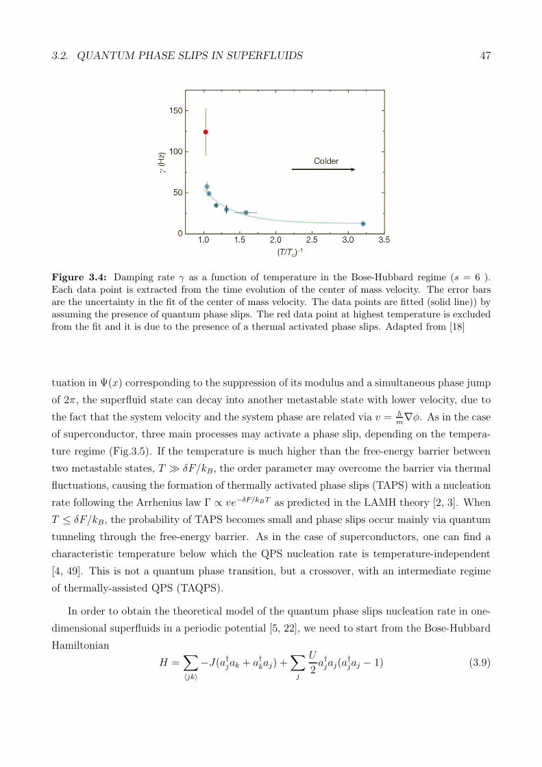
3.2. QUANTUM PHASE SLIPS IN SUPERFLUIDS 47
Figure 3.4: Damping rate γ as a function of temperature in the Bose-Hubbard regime (s = 6 ).Each data point is extracted from the time evolution of the center of mass velocity. The error barsare the uncertainty in the fit of the center of mass velocity. The data points are fitted (solid line)) byassuming the presence of quantum phase slips. The red data point at highest temperature is excludedfrom the fit and it is due to the presence of a thermal activated phase slips. Adapted from [18]
tuation in Ψ(x) corresponding to the suppression of its modulus and a simultaneous phase jump
of 2π, the superfluid state can decay into another metastable state with lower velocity, due to
the fact that the system velocity and the system phase are related via v = ~
m∇φ. As in the case
of superconductor, three main processes may activate a phase slip, depending on the tempera-
ture regime (Fig.3.5). If the temperature is much higher than the free-energy barrier between
two metastable states, T ≫ δF/kB, the order parameter may overcome the barrier via thermal
fluctuations, causing the formation of thermally activated phase slips (TAPS) with a nucleation
rate following the Arrhenius law Γ ∝ ve−δF/kBT as predicted in the LAMH theory [2, 3]. When
T ≤ δF/kB, the probability of TAPS becomes small and phase slips occur mainly via quantum
tunneling through the free-energy barrier. As in the case of superconductors, one can find a
characteristic temperature below which the QPS nucleation rate is temperature-independent
[4, 49]. This is not a quantum phase transition, but a crossover, with an intermediate regime
of thermally-assisted QPS (TAQPS).
In order to obtain the theoretical model of the quantum phase slips nucleation rate in one-
dimensional superfluids in a periodic potential [5, 22], we need to start from the Bose-Hubbard
Hamiltonian
H =∑
〈jk〉−J(a†jak + a†kaj) +
∑
j
U
2a†jaj(a
†jaj − 1) (3.9)

48 CHAPTER 3. PHASE SLIPS IN ONE DIMENSIONAL SYSTEMS
Quantum
phase slips
F
(a) Thermally activated
phase slips
(c)(b)
Thermally assisted
quantum phase slips
T* Ej/kB v/vc Ej/kB T
Figure 3.5: Cartoon of the phase slips activation mechanisms. a) At low temperatures, phase slipsare activated by quantum tunneling; b) by increasing the temperature, the quantum phase slips areassisted by the temperature. c) At large temperatures, phase slips are activated only by thermalfluctuations.
where a†j and aj are the boson creation and annihilation operators at the lattice site j, 〈jk〉indicates pairs of nearest neighbours, J is the single-particle hopping amplitude and U is the
on-site repulsive interaction energy. In the limit of large filling, the Hamiltonian can be mapped
into the O(2) quantum rotor model
H =∑
〈jk〉−2Jn cos (φk − φj) +
∑
j
U
2n2j (3.10)
where, n us the average number of bosons per site, φj and nj are the conjugate phase and
the number of particles on the site j. The importance of the quantum rotor model is due to
the fact that it is possible to apply the instanton techniques on this model and by using the
celebrated instanton formula [70, 71]
Γ ∝ e−S (3.11)
it is possible to analytically predict the quantum phase-slip nucleation rate Γ. Here S is the
action for the bounce solution (instanton) of the classical equations of motion. For momentum
lower than the critical velocity for breaking superfluidity in a periodic potential, vc, the quantum
phase slips nucleation rate depends on the velocity via
Γ ∝ vα (3.12)
where the parameter α depends on the interaction and it is equal to α = 2K − 2 with K the

3.2. QUANTUM PHASE SLIPS IN SUPERFLUIDS 49
Luttinger parameter [5]. As it has discussed before, there is not a quantum phase transition
from TAPS and QPS regime, but there is a crossover, characterized by a crossover temperature
T ∗, where quantum phase slips are assisted by the temperature (TAQPS). In this situation, the
nucleation rate of TAQPS depends also on the temperature T via
Γ ∝ vT α(γ)−1. (3.13)
Obviously, the specific form of δF and T ∗ depends on the specific type of obstacle experi-
enced by the superflow, e.g. disorder [72], isolated defects [6] or periodic potentials [5]. In the
case of ultracold quantum gases, the most controllable obstacles are optical lattices and in this
situation the free energy barrier is
δF ≃ Ej, (3.14)
with Ej = ~vs/√2d is the Josephson plasma energy and vs the sound velocity, and the crossover
temperature is
T ∗ ≃ Ej
kb
v
vc. (3.15)
The presence of phase slips strongly modifies the transport properties of a system, especially
in 1D where the effect of thermal and quantum phase slips is significant. Experiments performed
to study the transport properties of trapped gases in the presence of an obstacle, such as random
[73, 74], single barrier [75], or periodic potentials [66, 76, 77, 78, ?], have shown that dipole
oscillations, induced for example by a sudden displacement of a parabolic trap, are strongly
damped, even if the system is in the superfluid state. Theory provides a direct relation between
the damping rate G of the dipole oscillations and the phase-slip nucleation rate
G(v) ∝ Γ(v)
v(3.16)
by using both qualitative consideration on energy loss during the damping, which will be shown
in the following, and exact numerical simulations with time-evolving block decimation method
at zero temperature [22].
The energy loss during the damping can be written in two different ways. The first one
considers the energy loss due to the loss of potential energy in the first half period, which can
be written as
Eloss =1
2Mω2(A2
0 − A21), (3.17)
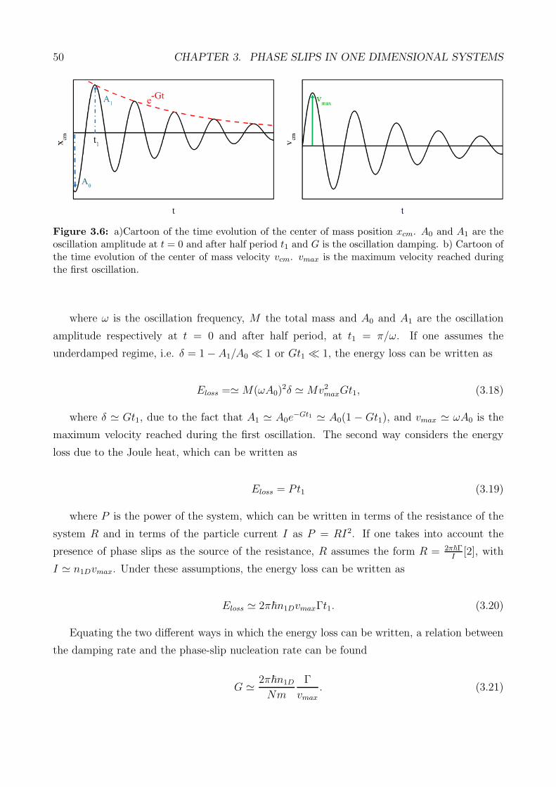
50 CHAPTER 3. PHASE SLIPS IN ONE DIMENSIONAL SYSTEMS
Figure 3.6: a)Cartoon of the time evolution of the center of mass position xcm. A0 and A1 are theoscillation amplitude at t = 0 and after half period t1 and G is the oscillation damping. b) Cartoon ofthe time evolution of the center of mass velocity vcm. vmax is the maximum velocity reached duringthe first oscillation.
where ω is the oscillation frequency, M the total mass and A0 and A1 are the oscillation
amplitude respectively at t = 0 and after half period, at t1 = π/ω. If one assumes the
underdamped regime, i.e. δ = 1− A1/A0 ≪ 1 or Gt1 ≪ 1, the energy loss can be written as
Eloss =≃ M(ωA0)2δ ≃ Mv2maxGt1, (3.18)
where δ ≃ Gt1, due to the fact that A1 ≃ A0e−Gt1 ≃ A0(1 − Gt1), and vmax ≃ ωA0 is the
maximum velocity reached during the first oscillation. The second way considers the energy
loss due to the Joule heat, which can be written as
Eloss = Pt1 (3.19)
where P is the power of the system, which can be written in terms of the resistance of the
system R and in terms of the particle current I as P = RI2. If one takes into account the
presence of phase slips as the source of the resistance, R assumes the form R = 2π~ΓI
[2], with
I ≃ n1Dvmax. Under these assumptions, the energy loss can be written as
Eloss ≃ 2π~n1DvmaxΓt1. (3.20)
Equating the two different ways in which the energy loss can be written, a relation between
the damping rate and the phase-slip nucleation rate can be found
G ≃ 2π~n1D
Nm
Γ
vmax. (3.21)

3.2. QUANTUM PHASE SLIPS IN SUPERFLUIDS 51
Figure 3.7: a) Scheme of the Damping rate G parameter dependence. G is velocity-dependent inthe QPS regime, it is temperature dependent in the TAQPS regime and it is defined by an Arrheniustype equation in the TAPS regime. b) Damping rate G as a function of the velocity in the presenceof quantum phase slips (pure and thermally assisted). Adapted by [22].
Consequently, as the phase-slip nucleation rate Γ, also the damping rate G behaves differ-
ently in the case of thermal or quantum fluctuations, as it is shown in Fig.3.7.
In the presence of TAPS, the damping rate G is defined by an Arrhenius type equation
G ∝ e−δFkBT (3.22)
and it shows a dependence on the temperature in the exponent, whereas in the case of QPS
it is temperature-independent and it depends on the velocity via
G ∝ vα−1 (3.23)
and it is temperature independent. In the intermediate case of QPS assisted by the temper-
ature, the damping rate G behaves differently from the QPS case: it is velocity independent
and it depends only on the temperature via
G ∝ T α−1. (3.24)
Another simple way to derive the relation between the damping rate G and the nucleation
rate Γ is the following. The deceleration at the first maximum in the oscillation can be written
in terms of the damping rate G as dv/dt = −Gv. In terms of individual phase slips, instead,
this can be written as δv/δt, where δv = −h/mL is the deceleration following a phase slip of
2π in a chain of length L and δt−1 = Γ. By equalling the two expressions we obtain again the
relation G = hmL
Γv.

52 CHAPTER 3. PHASE SLIPS IN ONE DIMENSIONAL SYSTEMS
Chapter 4
Exploring quantum phase slips in 1D
bosonic systems
4.1 Experimental procedure
The goal of my thesis is to study the transport properties of 1D bosonic superfluids in an
optical lattice, by focusing on how interaction and temperature affect the system behaviour.
In our experiments we employ 39K atoms which have a negative background scattering length,
i.e. abg = −44a0, and a broad Feshbach resonance[79], which gives us the possibility to tune
the interactions among the particles, as shown in sec. 1.3. The production of a 39K BEC is
not trivial: due to the level structure of this atom and its collisional properties in the absence
of a magnetic field, it is difficult to cool by evaporative cooling down to the temperature
necessary for the condensation [80]. As a consequence, we use sympathetic cooling with the87Rb atoms in order to obtain the BEC. In particular, we initially trap the atoms in a magnetic
optical trap where we perform the laser cooling in order to reach samples temperature (both
Rb and K) of the order of hundreds of microkelvin. Than, the atoms are trapped in a magnetic
trap where an evaporative cooling of Rb is performed, in order to obtain the temperature of
few microkelvin. Finally, the atoms are transferred in an optical trap, where we can use the
Feshbach resonance, and they can reach the right temperature for the condensation (few tens of
nK) after an additional evaporative cooling for the rubidium atoms and a sympathetic cooling
for the potassium atoms. In the following I will explain briefly the steps performed to achieve
the condensation. More details can be found in the previous thesis of my group [81, 83, 82].
Laser cooling in a MOT: The first step to obtain the 39K BEC is to cool the atoms
thanks to the laser cooling and to trap them into a magnetic optical trap (MOT).
53
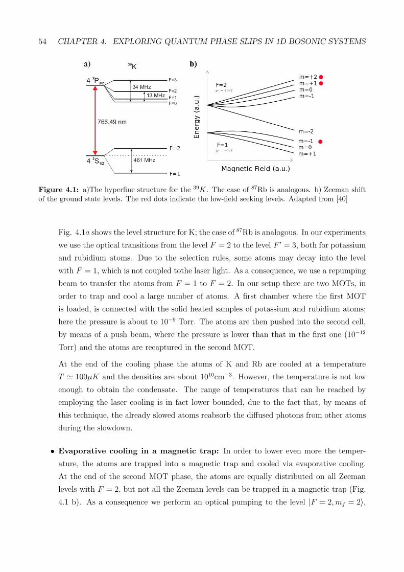
54 CHAPTER 4. EXPLORING QUANTUM PHASE SLIPS IN 1D BOSONIC SYSTEMS
Figure 4.1: a)The hyperfine structure for the 39K. The case of 87Rb is analogous. b) Zeeman shiftof the ground state levels. The red dots indicate the low-field seeking levels. Adapted from [40]
Fig. 4.1a shows the level structure for K; the case of 87Rb is analogous. In our experiments
we use the optical transitions from the level F = 2 to the level F ′ = 3, both for potassium
and rubidium atoms. Due to the selection rules, some atoms may decay into the level
with F = 1, which is not coupled tothe laser light. As a consequence, we use a repumping
beam to transfer the atoms from F = 1 to F = 2. In our setup there are two MOTs, in
order to trap and cool a large number of atoms. A first chamber where the first MOT
is loaded, is connected with the solid heated samples of potassium and rubidium atoms;
here the pressure is about to 10−9 Torr. The atoms are then pushed into the second cell,
by means of a push beam, where the pressure is lower than that in the first one (10−12
Torr) and the atoms are recaptured in the second MOT.
At the end of the cooling phase the atoms of K and Rb are cooled at a temperature
T ≃ 100µK and the densities are about 1010cm−3. However, the temperature is not low
enough to obtain the condensate. The range of temperatures that can be reached by
employing the laser cooling is in fact lower bounded, due to the fact that, by means of
this technique, the already slowed atoms reabsorb the diffused photons from other atoms
during the slowdown.
Evaporative cooling in a magnetic trap: In order to lower even more the temper-
ature, the atoms are trapped into a magnetic trap and cooled via evaporative cooling.
At the end of the second MOT phase, the atoms are equally distributed on all Zeeman
levels with F = 2, but not all the Zeeman levels can be trapped in a magnetic trap (Fig.
4.1 b). As a consequence we perform an optical pumping to the level |F = 2, mf = 2〉,

4.1. EXPERIMENTAL PROCEDURE 55
which is a low-field seeking state, and then we load the K and Rb mixture in a pure
magnetic trap with a QUIC configuration. The evaporative cooling is forced by removing
selectively the hottest atoms of Rb with a microwave transition into the high-field seek-
ing state |F = 1, mF = 1〉. In fact, in this level, the atoms are no longer trappable and
hence they are lost (Fig. 4.1 b). Rb is cooled down via evaporative cooling to T ≃ 1µK,
while K is sympathetically cooled via K-Rb collisions, without relevant atom losses. It
is important to know that after the forced and selective evaporation of Rb atoms on the
microwave transition, some Rb atoms survive in the state |F = 2, mF = 1〉 and they can-
not be cooled. As a consequence, it is necessary to use another frequency to eliminate
these atoms in order to reach the temperatures necessary to have a condensate.
Optical trapping and evaporation in the optical trap: In order to further cool down
the potassium atoms and to reach the condensation temperature, we transfer K and Rb
atoms into a dipole trap, which is realized with two crossed laser beams at a wavelength
λ = 1064 nm, which provide an average trap frequency of about 50 Hz. When the atoms
are trapped into the dipole trap, they are transferred from the state with |F = 2, mf = 2〉into the ground state with |F = 1, mf = 1〉. In this state K atoms are characterized by
an intraspecies Feshbach resonance at B0 ≃ 400 G and interspecies Feshbach resonance
with Rb and K atoms at B0 ≃ 315 G (4.2). The remaining Rb atoms into the level
|F = 2, mf = 2〉 are removed by using resonant light pulse. The optical evaporation of
the atoms is performed in two step, by exponentially lowering the intensity of the two
trap beams. During the first part, a homogeneous magnetic field is turned on at the value
B = 316 G, in order to increase the collisions between Rb and K atoms and to obtain
a more efficient thermalization between the two species. The shape of the evaporation
ramps has been chosen in order to obtain evaporation mostly on the vertical direction.
In this way we lose mainly the heavier rubidium atoms. In the second part, the intensity
of the two trap beams is lowered again until it reaches a vertical depth that allows the
formation of a pure K condensate. In this situation, the heavy rubidium atoms cannot
be trapped anymore and they are completely lost. In this phase, the magnetic field is
increased to the value B = 395 G, in order to increase the K scattering length and the
intraspecies collisions. At the end of the evaporation we have a 39K condensate, which is
characterized by a number of atoms of N and a temperature T .

56 CHAPTER 4. EXPLORING QUANTUM PHASE SLIPS IN 1D BOSONIC SYSTEMS
Figure 4.2: Heteronuclear (blue line) and homonuclear (black line) scattering lengths as a functionof the magnetic field. At B = 316 G the 39K atoms have a interspecies Feshbach resonance with the87Rb atoms whereas at B = 395 G the 39 K atoms have a intraspecies Feshbach resonance.Adaptedfrom [40].
4.2 Realization of 1D systems
We realize the 1D systems by splitting the 3D Bose-Einstein condensate with Ntot ≃ 30000
atoms by using a strong horizontal 2D optical lattice (with depth 20 ER). More in detail, the
2D lattice is ramped up in a fixed time (t = 400 ms) such that an array of independent potential
tubes direct along the vertical z axis is created, as it is shown in Fig. 4.3. In our conditions,
few hundred subsystems are created and each subsystem contains an average of 30-40 atoms.
The radial trapping energy ~ω⊥ = h × 40 kHz is much larger than all other energy scales,
realizing effectively 1D system. Along the longitudinal direction z, a 1D optical lattice with a
lattice spacing d = 532 nm is then added. The potential depth V0 can be tuned in the range
from s = V0/ER = 1 to s = 5, where ER = ~2k2/2m is the recoil energy, with k = π/d the
lattice wave vector. Along the z direction a harmonic potential (ωz = 2π × 150 Hz), required
from an experimental point of view to realize the 1D systems, is also present.
Due to the presence of the harmonic trap during the loading of the 2D lattice, the atoms
prefer to stay into the center of the trap rather than being distributed in an isotropic way,
making our system inhomogeneous. As a consequence, when we split the 3D BEC into a
matrix of 1D systems, we obtain that the most populated tubes are those at the centre of the
external optical trap.
At the same time, the gaussian laser beams that we employ to realize the 2D optical lattice

4.2. REALIZATION OF 1D SYSTEMS 57
Figure 4.3: The 1D systems are realized by splitting the 3D BEC into few hundreds of tubes byusing 2D deep optical lattices in the horizontal plane. Along the z direction a 1D optical lattice anda harmonic potential trap are present. Figure adapted from [84]
induce an inhomogeneity not on the full system scale as the harmonic trapping potential, but
in each 1D tube: in each 1D system, in fact, the density of bosons is greater in the centre
of the tubes due to the fact that in the presence of the external harmonic confinement, the
energy levels of the system are modified. In particular, if the interaction energy Eint between
the atoms is lower than the trapping energy, the particles prefer to share the same lattice site
rather than occupy different sites. As a consequence, due to the fact that the energy of the
external lattice site due to the harmonic trap is higher respect the energy of the central sites,
the more favourable energetic configuration is that where the atoms occupies the central sites
of the lattice.
In order to change the interparticle interaction, we tune the 1D scattering length a1D by
using a magnetic field, as it was shown in sec 2.2. The value of the scattering length aload
when the lattices are loaded determines the size of the condensate, therefore also the number
of populated tubes and the number of atoms in each tube. In particular, in the tube (i,j) the
number of atoms is given by
Ni,j = N0,0
[
1− 2πN0,0(i2 + j2)
5Ntot
]3/2
. (4.1)
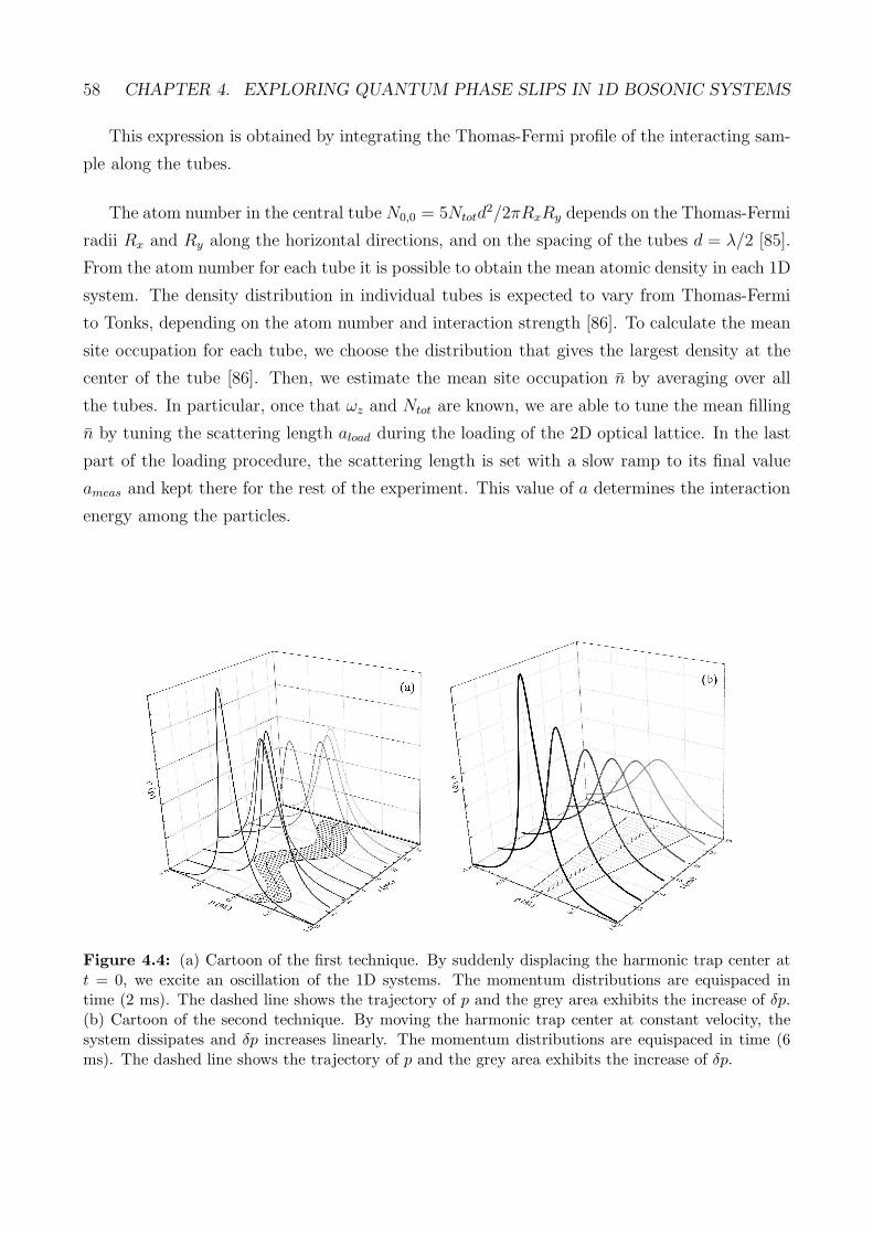
58 CHAPTER 4. EXPLORING QUANTUM PHASE SLIPS IN 1D BOSONIC SYSTEMS
This expression is obtained by integrating the Thomas-Fermi profile of the interacting sam-
ple along the tubes.
The atom number in the central tube N0,0 = 5Ntotd2/2πRxRy depends on the Thomas-Fermi
radii Rx and Ry along the horizontal directions, and on the spacing of the tubes d = λ/2 [85].
From the atom number for each tube it is possible to obtain the mean atomic density in each 1D
system. The density distribution in individual tubes is expected to vary from Thomas-Fermi
to Tonks, depending on the atom number and interaction strength [86]. To calculate the mean
site occupation for each tube, we choose the distribution that gives the largest density at the
center of the tube [86]. Then, we estimate the mean site occupation n by averaging over all
the tubes. In particular, once that ωz and Ntot are known, we are able to tune the mean filling
n by tuning the scattering length aload during the loading of the 2D optical lattice. In the last
part of the loading procedure, the scattering length is set with a slow ramp to its final value
ameas and kept there for the rest of the experiment. This value of a determines the interaction
energy among the particles.
Figure 4.4: (a) Cartoon of the first technique. By suddenly displacing the harmonic trap center att = 0, we excite an oscillation of the 1D systems. The momentum distributions are equispaced intime (2 ms). The dashed line shows the trajectory of p and the grey area exhibits the increase of δp.(b) Cartoon of the second technique. By moving the harmonic trap center at constant velocity, thesystem dissipates and δp increases linearly. The momentum distributions are equispaced in time (6ms). The dashed line shows the trajectory of p and the grey area exhibits the increase of δp.
4.3. EXCITING THE 1D MOTION 59
4.3 Exciting the 1D motion
As it was introduced it sec 2.3, the experimental observable is the momentum distribution
ρ(p), which is obtained performing time-of-flight absorption imaging, i.e. by releasing the
atomic cloud from all potentials and letting it free to expand before the image acquisition. By
fitting ρ(p) with a Lorentzian function, we are able to measure the quasimomentum p, which
we identify with the averaged momentum acquired by the atoms, and the half-width-at-half-
maximum δp.
In order to probe the transport properties of our systems we perform transport measurements,
by employing two different procedures. The first procedure consists in suddenly displacing the
center of the trap by abruptly switching off the magnetic field gradient which compensate for
gravity. The atoms are no longer in the minimum of the potential and start to oscillate in the
new potential configuration. After a variable evolution time, we record ρ(p) and we study the
time evolution of p, which is affected by the presence of dissipation (Fig. 4.4a). By tuning
the magnetic field gradient, we change the trap displacement and we excite oscillations with
different amplitude.
The second procedure consists in displacing the center of the trap at constant velocity by
linearly changing the magnetic field gradient. After a variable time in the trap, we record
ρ(p) (Fig. 4.4b). In this kind of measurements, we investigate the time evolution of δp, whose
increase is related to the dissipation. The energy dissipated during the harmonic potential
movement is in fact converted into momentum spread. In fig. 4.5 a scheme of the magnetic
field gradient behaviour for both procedures is shown.
Both procedure can be better understood by considering the analogous in the electric circuits
physics. The first procedure is analogous to excite an oscillation into an RLC circuit. Initially,
the electric circuit is at the equilibrium and there is not charge transport into the circuit.
Subsequently, a current start to flow with a sinusoidal behaviour when the capacitor is charged
and / or a current is induced in the inductor: this correspond to the sudden shift of the
harmonic trap. As in the case of our system, also in the case of a RLC circuit, if there is a finite
resistance, the current does not keep oscillating forever, but the oscillation amplitude slowly
diminishes with time and eventually the motion stops altogether. In the second procedure we
instead impose a constant velocity. This is analogous to imposing a continuous current into a
circuit. In both of the system we observe a Joule heating.

60 CHAPTER 4. EXPLORING QUANTUM PHASE SLIPS IN 1D BOSONIC SYSTEMS
4.4 Dissipation in the presence of oscillations: evidence
of quantum phase slips
In this section we will focus the attention on the experiments with an oscillating system. As
it was explained in the previous section, the oscillations are induced by suddenly shifting the
center of the harmonic trap. By working in the semiclassical framework, the oscillating motion
of the system in the trap in the presence of an optical lattice can be obtained by solving the
system of equations
p = −kez − βz
p = m∗(p)z
The first equation describes a damped oscillation along the z direction; it contains the coef-
ficients ke and β which are the elastic constant and the viscous friction coefficient, respectively.
The first term, ke, is related to the axial trapping frequency ωz via ωz =√
ke/m, whereas the
second coefficient, β, is related to the damping rate G via G = β/2m. The damping rate G is
a parameter of interest, which gives informations about the dissipation in the system.
The second equation takes into account the presence of an optical lattice in the effective
mass m∗ term, which is related to the curvature of the energy band of the lattice, as it was
shown in sec. 1.5.2.
grad
B (a
.u.)
t (a.u.)
"kick" measurements constant v measurements
Figure 4.5: Scheme of the magnetic field gradient behaviour for both experimental proceduresemployed to perform transport measurements. In the first procedure (solid black line) we abruptlyswitch off the magnetic field gradient which compensate the gravity in order to excite the systemoscillation. In the second one (red dashed line) we change linearly the magnetic field gradient in orderto perform measurements at constant velocity.

4.4. DISSIPATION IN THE PRESENCE OF OSCILLATIONS 61
In the presence of an optical lattice, both the oscillation frequency and the damping
depends on the effective mass m∗. In particular, the oscillation frequency takes the form
ω′ =√ω∗2 − 4πG∗2, where ω∗ = ωz
√
mm∗ is the oscillation frequency in the absence of any
dissipative effect, and G∗ = G mm∗ is the damping rate in the presence of the lattice.
In the presence of a finite damping rate G∗, the time evolution of p can be approximated
with a damped oscillation function of the form
p = m∗ve−Gt sin(ω′t+ ϕ) (4.2)
with amplitude p0(t) = m∗v = m∗ω∗2∆z/ω′ and frequency ω′ =√ω∗2 − 4π2G2. Here ∆z is
the trap displacement.
It is important to know that the system behaves according to the eq. 4.2 only if the
maximum momentum reached during the oscillation is smaller than the critical momentum for
the dynamical instability pc. If p < pc we observe a damping in the oscillations which is due to
the presence of phase slips.
For momenta larger than pc the system behaves differently from the previous case and the
system does not oscillate anymore. We observe, instead, an overdamped motion, which we
attribute to the occurrence of the dynamical instability that can be described in term of a
divergence of the phase-slips rate at the critical velocity vc of the superfluid.
In the subsection 4.4.1 we will treat the phenomenon of the dynamical instability, whereas
we will focus on the phenomenon of phase slips in the subsection 4.4.2.
4.4.1 Dynamical instability
A time evolution of the momentum distribution peak p for s = 2 and for a = 8.4a0 is shown in
Fig. 4.6 a. In this picture, we observe an initial increase of p up to a certain critical value pc,
which is followed by a subsequent decrease. More in detail, for p < pc, the oscillation is weakly
damped and the data points can be fitted by using the damped oscillation equation shown in
the previous section (Eq.4.2). This behaviour is consistent with the presence of phase slips, as
we will see more in details in the next subsection. For p > pc, instead, the system enters into a
dynamically unstable regime driven by a divergence of the phase slip rate, and the oscillation is
strongly damped. In order to estimate the critical momentum pc, which separates the weakly
dissipated regime from the strongly unstable one, we plot the difference between the fit of the
weakly damped oscillation and the experimental data, as shown in Fig. 4.6 b. In fact, the critical
momentum pc for the occurrence of the dynamical instability is identified as the value where the
experimental data points deviate with respect to the theoretical curve. The interception of the
62 CHAPTER 4. EXPLORING QUANTUM PHASE SLIPS IN 1D BOSONIC SYSTEMS
two linear fits identifies the time at witch the system enters the unstable regime, corresponding
to the critical momentum pc. We also observe the presence of two different regimes into time
evolution of the momentum distribution width δp: initially δp is almost constant, whereas it
abruptly starts increasing when the system enters into the unstable regime (Fig. 4.6 c)
This behaviour can be explained in terms of the phenomenon of the dynamical instability.
An intuitive explanation of this instability in the absence of interaction can be given in term
of the effective mass m∗.
As it was discussed in section 1.5.2, it is possible to describe the system dynamics in the
presence of an optical lattice by using the semi-classical model, provided that the mass of the
system is replaced with the effective mass m∗, which takes into account the presence of the
lattice. The effective mass is not constant, but it depends on the quasimomentum p of the
system, and, in particular, it can become negative at a certain value of the quasimomentum.
The critical value corresponds to one-quarter of the reciprocal lattice constant, i.e. π/2 at zero
interactions, only for a lattice strengths in the tight-binding regime (s ≥ 5).
When the effective mass of the system changes its sign, the BEC behaves as if it was subject
to a negative scattering length and, due to a such attractive interaction, the BEC collapses [87].
Another interpretation of this mechanism can be given in term of divergence of the phase
slips rate. When the system enters into the dynamical unstable regime, it is observed a rapid
growth of excitations (phase slips), which provoke a strongly dissipation and the system stops
oscillating. In this situation, the phase coherence of the system is broken due to the fact that
the tunnelling is not fast enough to lock the phases of adjacent sites, which start to run inde-
pendently. As a consequence, the system enters into an insulating incoherent regime.
So far we have considered the case of U = 0. For non-negligible interaction the situation
changes, and the critical momentum is not equal to π/2 (i.e. the theoretical value in the tight
binding regime). As it was shown in subsection 2.4.4, when the interaction among the particles
is strong enough to overcome the kinetic energy, the system undergoes a phase transition from
the SF to the MI regime, and this happens even for very small velocity. In this scenario, we thus
expect that the critical velocity decreases as the interactions increase, i.e. pc < π/2, vanishing
at the SF-MI transition [88].
As it is shown in Fig 4.7, we have excited the sloshing motion of the system for different
values of interactions and lattice depth. By increasing the scattering length, we observe that
the damping rate at short times increases, as the phase-slip nucleation rate increases (Fig. 4.7
a), while pc decreases (Fig. 4.7 b). However, as it is shown in Fig. 4.7 b, by increasing the
interactions, the measured pc reaches a finite constant value, but it does not vanish. The onset

4.4. DISSIPATION IN THE PRESENCE OF OSCILLATIONS 63
0,0 0,5 1,0 1,5 2,0 2,5 3,0 3,5 4,0-0,05
0,00
0,05
0,10
0,15
0,20
0,25
0,30
0,35
-0,5 0,0 0,5 1,0 1,5 2,0 2,5 3,0 3,5 4,0 4,5-0,05
0,00
0,05
0,10
0,15
0,20
0,25
0,0 0,5 1,0 1,5 2,0 2,5 3,0 3,5 4,00,12
0,14
0,16
0,18
0,20
0,22
0,24
0,26
p (
k)
t (ms)
p fit-p
(k)
t (ms)
p (
k)
t (ms)
Figure 4.6: (a) Time evolution of the momentum distribution peak p at s = 2 for a = 8.4a0. Thesolid line is the damped oscillation fitting the data for p < pc before the dynamical instability setsin. The blue circle marks the critical momentum pc. The error bars comprise the imaging resolutionand the statistical uncertainties. (b) Difference between the fit to the initial damped motion and theexperimental data (dots). The continuous line is the fit to estimate the critical momentum. (c) Timeevolution of the momentum width. The blue arrow marks the time t corresponding to the criticalmomentum pc.

64 CHAPTER 4. EXPLORING QUANTUM PHASE SLIPS IN 1D BOSONIC SYSTEMS
of this plateau can be interpreted as the critical scattering length ac to enter the Mott regime
for the commensurate regions of the system. As it was introduced in sec. 4.2, the presence of a
trap during the loading of the 2D lattice makes the 1D systems inhomogeneous and some tubes
contain commensurate regions, as well as incommensurate regions where the critical density
is always lower than unity. The transport along the tubes with a commensurate regions is
globally suppressed driving the system into an effective insulating regime, i.e. within in each
tube a part of the atoms reaches the localization condition n = 1 stopping also the remaining
adjacent parts with different occupation. The fraction of tubes that does not reach the critical
density n = 1 keeps instead moving also for a > ac, originating the observed plateau for pc. We
estimate that about one quarter of the atoms resides in tubes where the occupation is always
n < 1. For a given lattice depth when increasing the scattering length in the Mott phase,
a > ac, this fraction of delocalized atoms remains constant because in the tubes where the
Mott domains form, the density is fixed.
This interpretation seems confirmed by the observed increase of the plateau for decreasing
lattice depth (Fig. 4.7 b). In fact, the increase of the interaction strength that is necessary
to reach the insulating regime, produces an overall decrease of the density of the 1D systems,
hence an increase of the fraction of tubes that does not reach the critical density for the Mott
insulator transition. For each set of measurements with a given value of s, we determine the
0,0 0,5 1,0 1,5 2,0 2,5 3,0-0,05
0,00
0,05
0,10
0,15
0,20
0,25
0,30
0,35
0 50 100 150 200 250 300
0,10
0,15
0,20
0,25
0,30
206 a0
109 a0
45 a0
p (k)
t (ms)
s = 2 s = 4
p c(
k)
a (a0)
Figure 4.7: (a) Time evolution of the momentum distribution peak p at s = 2 for different valuesof scattering length. The solid lines are the theoretical damped oscillation fitting the data for p < pcbefore the dynamical instability sets in. The green circles mark the critical momentum pc. Theerror bars comprise the imaging resolution and the statistical uncertainties. (b) Critical momentumpc versus scattering length for two lattice depth: s = 4 (red squares) and s = 2 (black circles). Apiecewise fit (solid lines) determines the critical values for the SF-MI transition (empty circles) for n= 1: respectively ac/a0 = 122(8) (γc = 1.08(7)) and ac/a0 = 214(6) (γc = 1.88(5)).
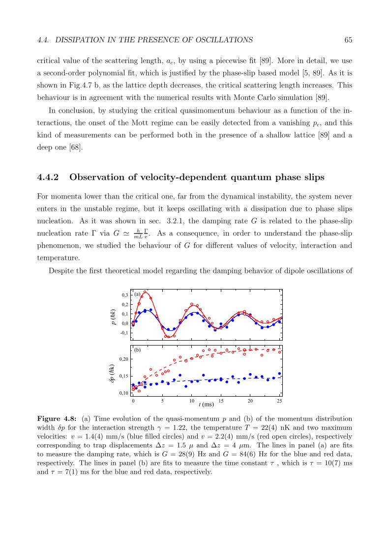
4.4. DISSIPATION IN THE PRESENCE OF OSCILLATIONS 65
critical value of the scattering length, ac, by using a piecewise fit [89]. More in detail, we use
a second-order polynomial fit, which is justified by the phase-slip based model [5, 89]. As it is
shown in Fig.4.7 b, as the lattice depth decreases, the critical scattering length increases. This
behaviour is in agreement with the numerical results with Monte Carlo simulation [89].
In conclusion, by studying the critical quasimomentum behaviour as a function of the in-
teractions, the onset of the Mott regime can be easily detected from a vanishing pc, and this
kind of measurements can be performed both in the presence of a shallow lattice [89] and a
deep one [68].
4.4.2 Observation of velocity-dependent quantum phase slips
For momenta lower than the critical one, far from the dynamical instability, the system never
enters in the unstable regime, but it keeps oscillating with a dissipation due to phase slips
nucleation. As it was shown in sec. 3.2.1, the damping rate G is related to the phase-slip
nucleation rate Γ via G ≃ hmL
Γv. As a consequence, in order to understand the phase-slip
phenomenon, we studied the behaviour of G for different values of velocity, interaction and
temperature.
Despite the first theoretical model regarding the damping behavior of dipole oscillations of
-0,1
0,0
0,1
0,2
0,3
0 5 10 15 20 250,10
0,15
0,20
p (
k)
(b)
(a)
p (
k)
t (ms)
Figure 4.8: (a) Time evolution of the quasi-momentum p and (b) of the momentum distributionwidth δp for the interaction strength γ = 1.22, the temperature T = 22(4) nK and two maximumvelocities: v = 1.4(4) mm/s (blue filled circles) and v = 2.2(4) mm/s (red open circles), respectivelycorresponding to trap displacements ∆z = 1.5 µ and ∆z = 4 µm. The lines in panel (a) are fitsto measure the damping rate, which is G = 28(9) Hz and G = 84(6) Hz for the blue and red data,respectively. The lines in panel (b) are fits to measure the time constant τ , which is τ = 10(7) msand τ = 7(1) ms for the blue and red data, respectively.

66 CHAPTER 4. EXPLORING QUANTUM PHASE SLIPS IN 1D BOSONIC SYSTEMS
one-dimensional ultracold gases due to the presence of phase slips [22] was performed in the
Bose-Hubbard regime, we have decided to study this phenomenon in the presence of a weak
optical lattice (V = 1ER). The reason is that we want to perform measurements far from the
dynamical instability, which occurs for velocity larger than a critical velocity, and to increase
the range of velocities investigated. In the previous chapter we have shown the behaviour of
the critical velocity for the dynamical instability for different values of interaction and lattice
depth. We have observed that, for a fixed interaction value, the critical velocity decreases as
the lattice depth increases (Fig. 4.7). As a consequence, by increasing the lattice depth, we
decrease the range of velocities that we can investigate far from the phenomenon dynamical
instability. In the presence of an optical lattice with depth s = 1, the critical velocity varies in
the range [0.74,0.56] ~k, depending on the interaction value.
The idea is that a weak lattice in the Sine-Gordon limit shifts the critical velocity towards
the band edge, thus enlarging the range of accessible v for studying the phase-slips phenomenon.
In the weak interaction limit, in fact, the critical velocity is defined as the point in which the
curvature of the Bloch band is zero, so that the critical velocity tends to the Bragg velocity for
vanishing lattice strengths.
The damping rate is measured by fitting the time evolution of p with the model presented
previously, as shown in Fig. 4.8. We observe that, at the same interaction γ = 1.22, the
damping rate G is different for two different values of velocity, which we identify in this kind of
measurements with the velocity reached during the first oscillation as in the theoretical model
[22], suggesting the presence of phase slips with a nucleation rate that depends on the velocity.
In fact, a small velocity v (blue filled circles) typically leads to a very weakly damped oscillation.
In this case, δp is almost constant showing that the system is just slighting dissipating and that
its coherence properties are almost preserved. Instead, at high velocity (red open circles), the
oscillation is strongly damped and δp greatly increases during the evolution, showing a strong
effect of excitations.
We fit the growth of δp with an inverted exponential,
δp(t) = δp(0) + p∞[1− exp(−t/τ)], (4.3)
where τ is the constant time and p∞ is the relative saturation value. We found that the damping
rate G is directly related to τ via 2τ ≃ 1/G, and this can be interpreted considering that the
mechanical energy dissipated in the oscillation is converted into momentum spread.
We have repeated this type of measurement for a wide range of velocities, interaction
strengths and temperatures. The temperature is estimated from the momentum distribution at

4.4. DISSIPATION IN THE PRESENCE OF OSCILLATIONS 67
0,2 0,3 0,4 0,5 0,6 0,7 0,8 0,90,2 0,3 0,4 0,5 0,6 0,7 0,8 0,930
60
90
120
150180210
T = 34 nK T = 43 nK
(b)
v/vc
20 30 40 500
30
60
90
G
(Hz)
T (nK)
a = 38 a0
a = 93 a0
G
(Hz)
v/vc
(a)
Figure 4.9: (a) Damping rate G is plotted versus the maximum velocity v normalized to the criticalvelocity vc, for three interaction strengths and constant temperature: γ = 0.13 and T = 37(7) nK(black circles), γ = 0.19 and T = 39(7) nK (orange triangles) and γ = 0.64 and T = 34(5) nK (bluesquares). (b) G versus v/vc for two different temperatures and approximately constant interactionenergy: T = 34(5) nK and γ = 0.64 (blue squares) and T = 43(5) nK and γ = 0.70 (red stars). Thelines are fits to measure the crossover velocity v∗ .
t = 0 and the mean atom number per site n via the established relation kBT = ~nδp0/0.64m∗d
[90, 91], where m∗ is the effective mass which takes into account the presence of an optical
lattice. In our measurements the temperature T changes from 20 to 35 nK and the interaction
strength γ changes form 0.13 to 1.22. Some measurements of the evolution of G with velocity
and interaction at the same temperature are shown in fig 4.9. Each data set is rescaled to the
corresponding critical velocity vc for dynamical instability, which is measured according to the
technique introduced in the previous subsection.
In Fig.4.9 a, two different datasets at the same temperature and different interaction are
reported. For strong interaction (orange, blue), we observe a clear crossover from a regime of
constant G to a regime where G grows with the velocity.
We fit the data by using a piece-wise linear function and we determine the crossover velocity
v∗, which we define as the minimum velocity required to enter the velocity-dependent regime.
The crossover velocity seems to depend on the interaction and in particular it apparently
decreases for increasing interaction.
By repeating the same measurements for different values of temperature and at the same
interaction, we observe a similar behaviour similar to the one introduced earlier (Fig. 4.9 b).
Also in this case, in fact, we observe a crossover from a regime where G is velocity independent

68 CHAPTER 4. EXPLORING QUANTUM PHASE SLIPS IN 1D BOSONIC SYSTEMS
0,4 0,6 0,8 1,0 1,2 1,4 1,6 1,8 2,0
0,10
0,15
0,20
0,25
0,30
0,35
e
dc
b
v* (k)
kBT/Ej
a
Figure 4.10: Crossover velocity as a function of the temperature normalized to the Josephson plasmaenergy. The crossover velocity increases as the temperature rises. The individual datapoints have beentaken for different temperatures and interaction energies: a) γ = 1.22 and T = 22(2) nK, b) γ = 0.64and T = 34(5) nK, c) γ = 0.37 and T = 30(5) nK, d) γ = 0.70 and T = 43(5) nK, e) γ = 0.19 and T= 39(7) nK.
to a regime where G grows with velocity.
Moreover, as shown in Fig. 4.9 b , in the regime where G does not depend on the velocity, i.e.
for v ≪ v∗, the damping rate G is strongly affected by temperature and we observe a monotonic
increase of G with T (as shown in the inset in Fig. 4.9 b). In this regime the dependence on
interaction (Fig. 4.9a) is weaker. On the contrary, in the v-dependent regime, interaction
effects are apparently dominant (Fig. 4.9 a), whereas we cannot measure a clear dependence
on T (Fig. 4.9 b). As a consequence of the combination of these effects, the crossover velocity
increases as the temperature increases. The behaviour of the crossover velocity as a function
of the temperature normalized to the Josephson plasma energy is shown in fig.4.10.
These observations appear consistent with the predicted crossover from a regime where the
nucleation of phase slips is due to thermal effect to a regime of quantum phase slips. We do not
control this crossover by changing the temperature T , but by varying the crossover temperature
T ∗ ∝ Ej/kBv/vc (4.4)
by tuning velocity and interaction strength. For T ∗ ≪ T , i.e. at small velocity and small
interaction, G depends only on T and it is velocity-independent, suggesting a thermal acti-
vation of phase slips. For T ∗ ≫ T , i.e. at large velocity and large interaction, the system

4.4. DISSIPATION IN THE PRESENCE OF OSCILLATIONS 69
0,5 1,0 1,5 2,0
0,2
0,3
0,4
0,5
T-dependent regime
e
dc
b
v-dependent regime
v* /vc
kBT/Ej
a
Figure 4.11: Crossover velocity v∗/vc versus kBT/Ej . The individual datapoints have been takenfor different temperatures and interaction energies: a) γ = 1.22 and T = 22(2) nK, b) γ = 0.64 andT = 34(5) nK, c) γ = 0.37 and T = 30(5) nK, d) γ = 0.70 and T = 43(5) nK, e) γ = 0.19 and T =39(7) nK. The dashed line apparently separates the thermal and the quantum regimes for phase slips.
enters in a regime where G is linearly dependent on the velocity and temperature independent,
suggesting a quantum activation of phase slips. A further indication that our measurements
are in agreement with the crossover from thermal assisted to quantum phase slips is the lin-
ear scaling of the crossover velocity normalized to the critical velocity v∗/vc as a function of
temperature normalized to the Josephson energy kBT/Ej. As shown in fig. 4.11, despite the
individual datapoints have been measured for scattered values of γ and T , they show a clear
linear scaling, which is consistent with the theoretical prediction
kBT∗
Ej∝ v
vc. (4.5)
From the fit we get the relation for the crossover velocity T ∗ as a function of v, Ej and vc
kBT∗ = 4.9(14)Ej
v
vc− 0.4(4)Ej. (4.6)
Unfortunately, the agreement with the theory is only qualitative since we cannot reproduce
the theoretical exponent α. In our experiments we observe a damping rate that is proportional
to T α−1 in the case of thermally activated phase slips and to vα in the quantum phase slips
one, but our experimental exponents α are interaction independent and they are of the order

70 CHAPTER 4. EXPLORING QUANTUM PHASE SLIPS IN 1D BOSONIC SYSTEMS
of unity [19], as it is shown in fig.4.12.
0,2 0,4 0,6 0,8 1,0 1,20
2
4
6
8
10
12
14
experimental exponents theorethical exponents
Figure 4.12: Experimental (red circles) and theoretical (black triangles) exponents α as a functionof the interaction γ. Our exponents are about constant (and of the order of the unit) and they do notdepend on the interaction. On the contrary, the theoretical exponents depend on the interaction andthey can be an order of magnitude larger than the experimental exponents.
On the contrary, according to the theoretical model [22], the theoretical exponents depend
on the interaction. By using the relation between the Luttinger parameter K and the Lieb-
Liniger parameter γ in the limit of no lattice potential (s = 0) and for small interactions
(γ < 10)
K ∼ π√
γ − γ3/2/(2π) (4.7)
we estimate the theoretical exponents and we find that they vary from about 13 to 4.5 in
the same range of interaction strengths, i.e. they can be an order of magnitude larger than
the measured exponents [22]. Possible reasons for the disagreement are the range of velocities
explored, much larger than in the theory , and the lattice strength (s = 1), much lower than in
the theory [22]. More in detail, the power-law behavior I showed above is valid only for very
low velocities (p < hk/10), while in the experimental range (hk/10 < p < hk/2) a different,
exponential behavior has been predicted [22, 5]. On the experimental side, the limited range
of accessible velocities, which is limited by the finite T on the low-v side, does not allow us to
distinguish a power law from an exponential.

4.4. DISSIPATION IN THE PRESENCE OF OSCILLATIONS 71
4.4.3 Comparison between our experimental results and the theo-
retical model of thermally activated phase slips of one-dimensional
Bose gases in the Sine Gordon limit.
Recently M.Kunimi and I. Danshita from the Yukawa Institute for Theoretical Physics, have
performed a theoretical study of thermally activated phase slips of one-dimensional Bose gases
in a shallow optical lattice, motivated by our experimental results.
They find, at low velocity and weak interaction, damping rates comparable with our experi-
mental values, by assuming the presence of thermal activated phase slips rather than thermally
assisted quantum phase slip [23]. In the following I will briefly show a summary of the methods
that they have used and a comparison between their theoretical and our experimental results.
Under the mean-field approximation, they initially consider a ring shape system with an
optical lattice and they estimate the energy barrier between the stable and the unstable solu-
tions of the stationary Gross-Pitaevskii equation, the frequency of the unstable mode and the
curvature of the energy landscape around the stationary solutions. By employing the Kramers
formula, they use the previous results to calculate the behaviour of nucleation rate of TAPS as
a function of the filling factor n = n1Dd and the velocity. Finally, they estimate the damping
rate G by using the local density approximation, in order to take into account the inhomo-
geneity of the system, due to the presence of an harmonic trap, and the temporal change of
the velocity. More in detail, to include these effects, they substitute the power P in the eq.
3.19 with the power per unit length P = P [n(x, t), v(t;G)] = 2π~Γ[n(x, t), v(t;G)]n(x, t)v(t;G)
at time t. Here, Γ = Γ/L is the nucleation rate per unit length. The spatial and temporal
dependences of the power and the nucleation rate is originated by the local particle density
n(t, x) = nTF (x− xcm(t)), which depends on the 1D Thomas-Fermi density profile nTF and on
the position of the center of mass during the damped oscillation xcm(t), and by the velocity
v(t;G) = e−Gtvmaxsin(ωLt).
In this scenario, the energy loss in eq. 3.19 can be substituted by
Eloss =
t1∫
0
dt
∫
dxP = P [n(x, t), v(t;G)] (4.8)
which is obtained by integrating the power P [n(x, t), v(t;G)]. By equaling Eq. 4.8 and
Eq. 3.17, with A1 ≃ A0e−Gt1 , they obtained a relation between the damping rate G and the
nucleation rate Γ
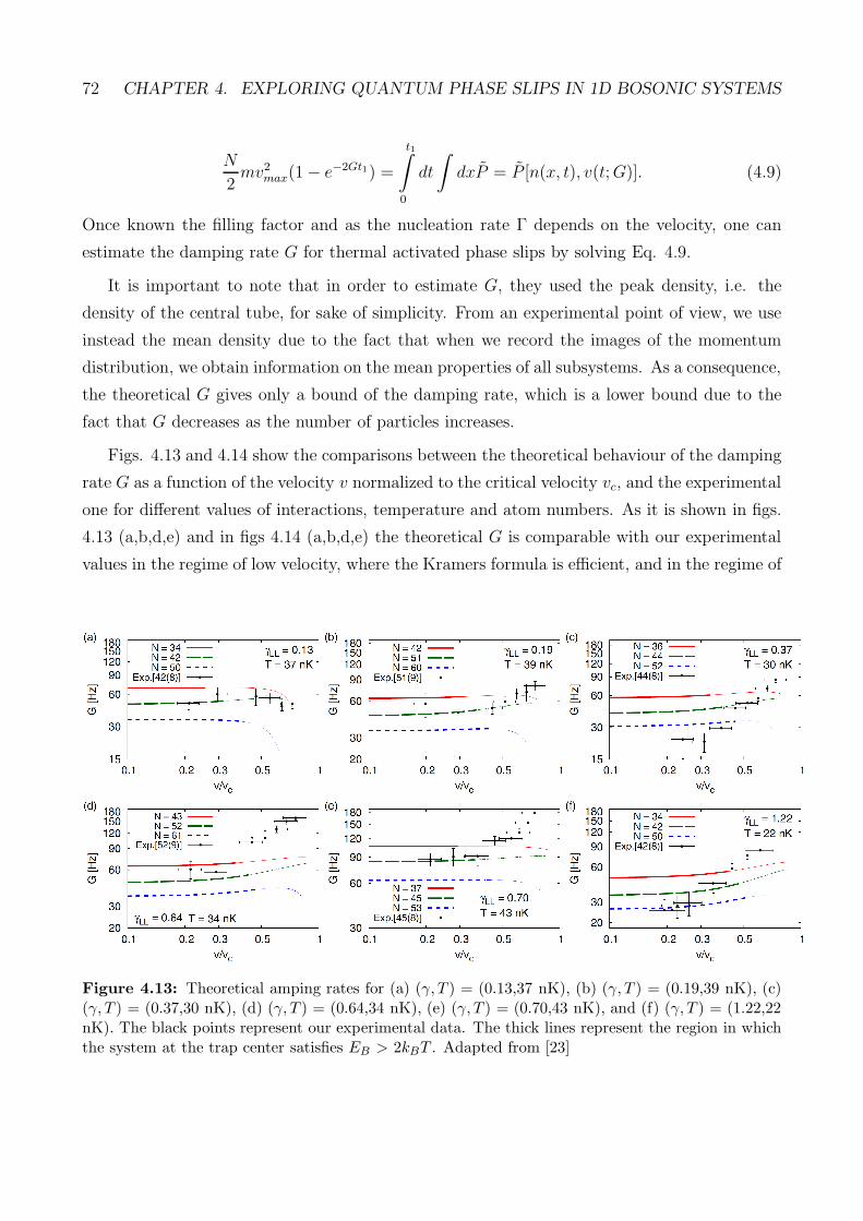
72 CHAPTER 4. EXPLORING QUANTUM PHASE SLIPS IN 1D BOSONIC SYSTEMS
N
2mv2max(1− e−2Gt1) =
t1∫
0
dt
∫
dxP = P [n(x, t), v(t;G)]. (4.9)
Once known the filling factor and as the nucleation rate Γ depends on the velocity, one can
estimate the damping rate G for thermal activated phase slips by solving Eq. 4.9.
It is important to note that in order to estimate G, they used the peak density, i.e. the
density of the central tube, for sake of simplicity. From an experimental point of view, we use
instead the mean density due to the fact that when we record the images of the momentum
distribution, we obtain information on the mean properties of all subsystems. As a consequence,
the theoretical G gives only a bound of the damping rate, which is a lower bound due to the
fact that G decreases as the number of particles increases.
Figs. 4.13 and 4.14 show the comparisons between the theoretical behaviour of the damping
rate G as a function of the velocity v normalized to the critical velocity vc, and the experimental
one for different values of interactions, temperature and atom numbers. As it is shown in figs.
4.13 (a,b,d,e) and in figs 4.14 (a,b,d,e) the theoretical G is comparable with our experimental
values in the regime of low velocity, where the Kramers formula is efficient, and in the regime of
Figure 4.13: Theoretical amping rates for (a) (γ, T ) = (0.13,37 nK), (b) (γ, T ) = (0.19,39 nK), (c)(γ, T ) = (0.37,30 nK), (d) (γ, T ) = (0.64,34 nK), (e) (γ, T ) = (0.70,43 nK), and (f) (γ, T ) = (1.22,22nK). The black points represent our experimental data. The thick lines represent the region in whichthe system at the trap center satisfies EB > 2kBT . Adapted from [23]

4.4. DISSIPATION IN THE PRESENCE OF OSCILLATIONS 73
Figure 4.14: Damping rates for (a) (γ,N) = (0.13,42), (b) (γN) = (0.19,51), (c) (γN) = (0.37,44),(d) (γN) = (0.64,52), (e) (γN) = (0.70,45), and (f) (γN) = (1.22,42). The black points representour experimental data. The thick lines represent the region in which the system at the trap centersatisfies EB > 2kBT . Adapted from [23]
Figure 4.15: Theoretical (red dots) and experimental (blue x) damping rate as a function of tem-perature for (γ,N) = (0.67,49). The error bars in the theoretical data points are estimated by thevalue of G at the lower and upper bounds of the experimental temperature, whereas the error bars inthe experimental data points represent the statistical uncertainties. Adapted from [23]
74 CHAPTER 4. EXPLORING QUANTUM PHASE SLIPS IN 1D BOSONIC SYSTEMS
weak interaction, where the GP mean-field theory is valid. This agreement suggests a thermal
nature of the phase slips and in particular for low velocity and weak interaction the damping in
the system oscillations seems be due to thermally activated phase slips, rather than thermally
assisted quantum phase slips.
In figs.4.13 (c,f) and figs. 4.14 (c,f), we see that our experimental data are not in agreement
with the theoretical model and in particular they are not included into the region between the
upper and lower theoretical curves. The disagreement in figs. 4.13 f and 4.14 f is probably
due to the fact that the interaction γ = 1.22 is too large to use the GP mean-field theory,
whereas the disagreement in figs. 4.13 c and 4.14 c is not clear. As shown in fig. 4.15, the
experimental values of G for different temperatures are in good agreement with the theoretical
values and this can be considered a further indication that in the regime of weak interaction
and low velocity the nature of phase slips is purely thermal. Nevertheless, it is still missing a
comparison for large velocity and large interaction regime, where the experiment observed a
damping rate G which depends on the velocity but not on the temperature. This behaviour is
compatible with a quantum activation of phase slips.
In conclusion, our results provide for the first time the experimental evidence of quantum
phase slips in one-dimensional superfluids, and consists also in the first observation of the
crossover from a regime of phase slips due to thermal fluctuation to a phase slips due to quantum
fluctuations. Moreover, in the regime of low velocities and low interactions, our measurements
are in agreement with the theoretical model for thermally activated phase slips. However, the
quantitative comparison between theory and experiment in the QPS regime is still missing.
One important feature of our setup is that the quantum regime can be reached at constant
temperature, by tuning the velocity or the interaction. This offers the possibility to control the
quantum phase-slip nucleation rate and opens new perspectives for the study of QPS-related
phenomena in ultracold quantum gases.
4.5 Dissipation at constant velocity: exploring the strongly
interacting regime
In this section I will describe a second series of experiments, where we have investigated the
dissipation during a shift of the trap at constant velocity. By employing this new experimental
technique, we have the advantage of being able to study the phase-slips dissipation rate at
interaction strengths larger than those investigated for oscillating systems.

4.5. DISSIPATION AT CONSTANT VELOCITY 75
As it was shown in the previous section, the range of velocity that can be investigated by
performing oscillation measurements is limited by the phenomenon of dynamical instability.
In particular, the critical velocity vc for this phenomenon limits above this range of velocity,
which decreases when the interaction increases as the critical velocity vc. As a consequence,
experimental measurements at lower velocity are required. Nevertheless, in the oscillation
measurements, the range of velocity is also limited below due to an experimental limit that
is related to the finite temperature of the system. In fact, if the velocities are too small, the
thermal effect provokes a finite damping which prevent the observation of a complete oscillation
and thus the measurement of the dissipation rate.
Instead, by shifting the trap at constant velocity we can extend the range of the velocities
investigated and, at the same time, also the range of interactions. The idea is the following:
by imposing the trap displacement at constant velocity, we are able not only to reach velocity
lower than those achieved in the case of an oscillating system, but we are also able to approach
velocity close to the critical velocity without ever reaching it. This is an important difference
respect tp the measurements performed with an oscillating system: here in fact the dynamical
instability occurs when the maximum velocity is close to the critical velocity, regardless of
whether the mean velocity of the system is lower than the critical one. Due to the fact that in
this kind of measurements we can impose the system velocity, we can perform measurements at
velocity chosen appropriately. As it was shown previously, in fact, by increasing the interactions
we decrease the critical velocity. As a consequence, we perform measurements at low velocity
in order to stay far from the dynamical instability also in the presence of a strongly interacting
system. In particular, while in the measurements shown in subsection 4.4.2 we have reached
the lowest maximum velocity of 1.2 mm/s and the highest interaction γ = 1.22, by shifting the
center of the trap at constant velocity we can reach a velocity of 0.4 mm/s and an interaction
γ = 8.4.
In the measurements performed by shifting the trap at constant velocity, the experimental
observable is the momentum spread. In particular we measure the dissipation rate from the
increase of the momentum spread, due to the fact that the energy dissipated during the system
dynamics is converted into momentum spread.
In this kind of measurements we expect that a superfluid should follow the trap displacement
and dissipate due to the presence of phase slips, resulting in an increase of δp. A Mott insulator
should not instead follow the trap displacement and should not dissipate, unless a trap shift
large enough to break the insulator is applied[24], as it will be explained more in detail in the
following subsection.
For a superfluid, the dissipation rate R is related to the nucleation rate of phase slips Γ and
76 CHAPTER 4. EXPLORING QUANTUM PHASE SLIPS IN 1D BOSONIC SYSTEMS
to the system velocity v via a relation of the form R ∝ vΓ.
This result can be obtained as follows. As it was shown in section 3.2.1, for a 1D system
of length L the rate of change of velocity due to the presence of phase slips is related to the
dissipation rate Γ via the relation
dv
dt=
−hΓ
mL. (4.10)
Therefore, for N particles, the rate of change of kinetic energy due to phase slips is
dEk
dt= Nmv
dv
dt= −NhvΓ/L. (4.11)
From this relation one obtains the energy dissipation rate
−dEk
dt= hρvΓ (4.12)
where ρ = N/L. By assuming the variation of the kinetic energy as an effective temperature,
and using the known relation between T and δp, [90, 91], we estimate a linear increase in time
of the momentum spread δp = δp0 +Rt, with a rate
R ≃ 4vm∗Γ. (4.13)
4.5.1 Shallow lattice
The first measurements that we have performed with this technique are in the presence of a
shallow lattice with s = 1, across the SF-MI transition, for a trap velocity of 0.8 mm/s. In
fig.4.16 the time evolution of δp for different values of scattering length is reported. We observe
that δp increases linearly with time, as expected. In particular, when the system is in the
superfluid phase, for γ < γc , δp is almost constant, showing that the system is just slightly
dissipating due to phase slips, and that its coherence properties are almost preserved. By
increasing the interaction, the system undergoes a phase transition to the insulator phase and
we observe that δp greatly increases during the evolution. It is important to remember that
the critical interaction for the transition from the superfluid phase to the insulating ones, γc, is
estimated independently by measuring the critical scattering length with the technique shown
in sec. 4.4.1 and by using the relation Eq. 2.23 between γ and g1D.
With a linear fit of the data we find the dissipation rate R, which increases by increasing the
interaction as shown in Fig. 4.16 b. In particular, the dissipation rate shows a roughly linear
dependence on the interaction, except for the point at very low interaction (γ = 0.038(4)). In

4.5. DISSIPATION AT CONSTANT VELOCITY 77
order to have an indication about the nature of the phase slips on the basis of the diagram in
fig. 4.11, we estimate T , Ej and vc when the system is in the superfluid regime. We find a
temperature T = 27±5 nK except for the data set at γ = 0.038(4) which is at T = 60±10 nK.
The higher temperature for the data set at the lowest interaction is probably due to the fact
that when we use a slow ramp to set aload to the final value ameas, we are not really adiabatic and
the system heats up. We find that the point at high temperature is in the T -dependent region
suggesting that its dissipation may be due to the presence of thermally activated phase slips. By
increasing the interaction, we find that the point at γ = 1.8 is close to the crossover between the
T -dependent region and the v-dependent one whereas the last point in the superfluid regime (γ
= 3.2) is in the v-dependent region, suggesting that the dissipation may be due to the presence
of quantum phase slips. Surprisingly, we observe a finite dissipation also when the system is
in the insulating regime, as shown in fig. 4.16. This dissipation may be due to two different
phenomena. The first phenomenon is related to the coexistence of a superfluid and a Mott
insulating phase, due to the inhomogeneity of our system. As it was described in sec. 4.2, the
presence of an harmonic trap, when splitting the BEC in an array of 1D tubes, makes our system
inhomogeneous and in particular we observe that the population decreases from the tubes in
the center of the array to the ones in the tails. As a consequence, we may have some tubes
reaching a commensurate filling and other ones where there are not commensurate regions. By
0 5 10 15 20 25 300,0
0,2
0,4
0,6
0,8
0 2 4 6 8 100
2
4
6
8
10
12
14
16
18
a = 494 a0
a = 379 a0
a = 260 a0
a = 11 a0
p (
k)
t (ms)
MI regime
R (
ks-1
)
200 300 400 5000,16
0,20
0,24
0,28
p c (
k)
a (a0)
SF regime
Figure 4.16: (a) Time evolution of the momentum width δp for s = 1 at various interaction strengths:γ = 0.038(4) (black circles), γ = 3.25(4) (cyan diamonds), γ = 5.55(4) (blue squares) and γ = 8.40(8)(red stars). Trap velocity v = 0.8 mm/s (i.e. ∆z = 24µm and t = 30 ms). Solid lines are linearfits to extract the dissipation rate R. (b) Dissipation rate versus the interaction strength for s =1. Inset: critical momentum versus scattering length. The piecewise fit (solid line) determines theexperimental critical value for the SF-MI transition (empty circle) ac/a0 = 392(12). The grey zoneindicates the superfluid regime, whereas the white zone the Mott insulator regime. The solid arrowmarks the experimental interaction value for the SF-MI transition (γc = 3.44(16)).
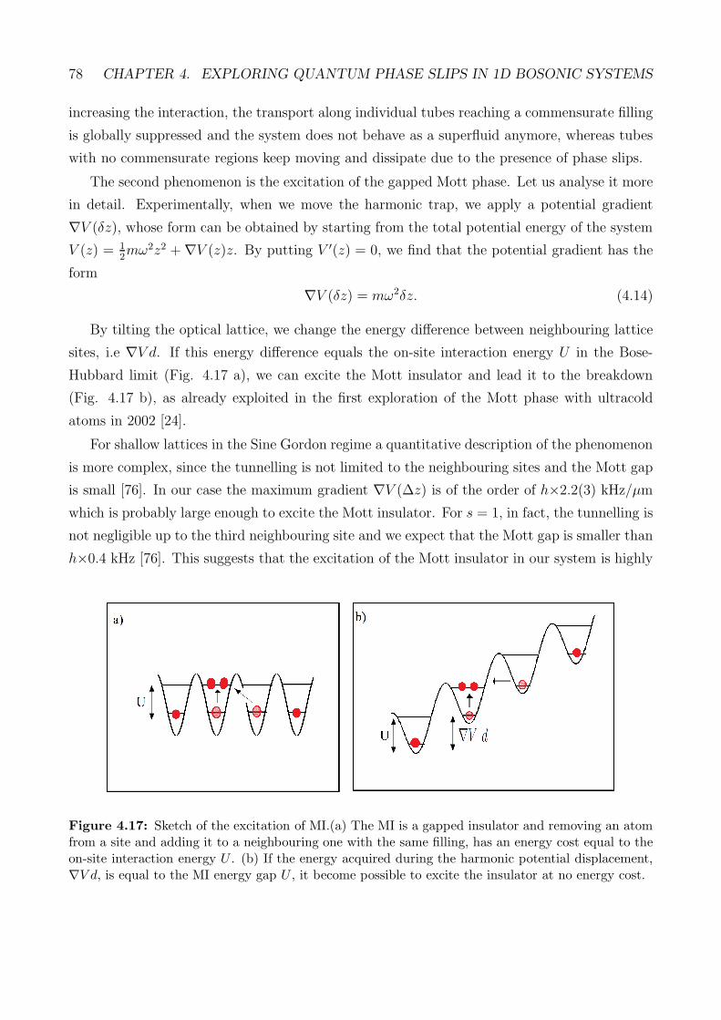
78 CHAPTER 4. EXPLORING QUANTUM PHASE SLIPS IN 1D BOSONIC SYSTEMS
increasing the interaction, the transport along individual tubes reaching a commensurate filling
is globally suppressed and the system does not behave as a superfluid anymore, whereas tubes
with no commensurate regions keep moving and dissipate due to the presence of phase slips.
The second phenomenon is the excitation of the gapped Mott phase. Let us analyse it more
in detail. Experimentally, when we move the harmonic trap, we apply a potential gradient
∇V (δz), whose form can be obtained by starting from the total potential energy of the system
V (z) = 12mω2z2 +∇V (z)z. By putting V ′(z) = 0, we find that the potential gradient has the
form
∇V (δz) = mω2δz. (4.14)
By tilting the optical lattice, we change the energy difference between neighbouring lattice
sites, i.e ∇V d. If this energy difference equals the on-site interaction energy U in the Bose-
Hubbard limit (Fig. 4.17 a), we can excite the Mott insulator and lead it to the breakdown
(Fig. 4.17 b), as already exploited in the first exploration of the Mott phase with ultracold
atoms in 2002 [24].
For shallow lattices in the Sine Gordon regime a quantitative description of the phenomenon
is more complex, since the tunnelling is not limited to the neighbouring sites and the Mott gap
is small [76]. In our case the maximum gradient ∇V (∆z) is of the order of h×2.2(3) kHz/µm
which is probably large enough to excite the Mott insulator. For s = 1, in fact, the tunnelling is
not negligible up to the third neighbouring site and we expect that the Mott gap is smaller than
h×0.4 kHz [76]. This suggests that the excitation of the Mott insulator in our system is highly
Figure 4.17: Sketch of the excitation of MI.(a) The MI is a gapped insulator and removing an atomfrom a site and adding it to a neighbouring one with the same filling, has an energy cost equal to theon-site interaction energy U . (b) If the energy acquired during the harmonic potential displacement,∇V d, is equal to the MI energy gap U , it become possible to excite the insulator at no energy cost.

4.5. DISSIPATION AT CONSTANT VELOCITY 79
probable. In the absence of a quantitative modelling it is not possible to discriminate which
one of the two effects dominates the observed dissipation. Further measurements, in a different
regimes, are required in order to understand which effect provokes the observed dissipation also
when the system is in the insulating phase. As a consequence, we decided to repeat this kind
of measurements in the Bose-Hubbard regime. In this situation, in fact, the Mott insulator
gap is well defined and we can compare it with the energy acquired during the harmonic trap
displacement.
4.5.2 Deep lattice
We have repeated this type of experiments at constant velocity in the presence of a deeper
lattice with s= 5. In this case we expect a clearer distinction between the Mott insulator and
superfluid fractions of the system, since in the Bose-Hubbard limit the Mott gap is larger and
the tunnelling is essentially only to the neighbouring sites.
In fig. 4.18 a the time evolution of δp, for a trap velocity of 0.4 mm/s and for different
values of scattering length, is shown. Also in this case we observe a linear scaling of δp with
0 5 10 15 20 250,10
0,15
0,20
0,25
0,30
0,35
0,40
0,45
0,50
0,55
0,60
0 2 4 6 8 10 12 14 16
-0,5
0,0
0,5
1,0
1,5
2,0
2,5
3,0
3,5
4,0
4,5
5,0(b) a = 38 a0
a = 94 a0
a = 213 a0
p (
k)
t (ms)
(a)
MIRegime
R (
k s-1
)
U/J
SFRegime
10 1000,05
0,10
0,15
0,20
0,25
0,30
p c (k)
a (a0)
Figure 4.18: (a) Time evolution of δp for s = 5 and different interaction strengths: U/J = 1.9(1)(blue triangles), U/J = 4.9(3) (red circles) and U/J = 12.3(7) (black squares)). The data set atU/J = 4.9(3) is shifted by 0.1 ~k and the data set at U/J = 12.3(7) is shifted by 0.2 ~k. Trapvelocity v = 0.4 mm/s (i.e. ∆z = 10µm and t = 25 ms). The solid lines are linear fits to extract thedissipation rate R. The data set at U/J = 4.9(3) show an activation mechanism, i.e. for t > t∗ ≃ 20ms the time evolution of δp can be fitted with a linear function with a larger slope (dashed line).(b) Dissipation rate R versus the interaction strength for s = 5. Inset: critical momentum versusscattering length. The piecewise fit (solid line) determines the experimental critical value for the SF-MI transition (empty circle) ac/a0 = 85(15). The grey zone indicates the superfluid regime, whereasthe white zone the Mott insulator regime. With the solid arrow we mark the experimental interactionvalue for the SF-MI transition (γc = 4.5(3)).

80 CHAPTER 4. EXPLORING QUANTUM PHASE SLIPS IN 1D BOSONIC SYSTEMS
time, in both superfluid and Mott insulator regimes. We now calculate that the Mott gap U/h
varies from 2.2(2) to 4.2(3) kHz, while the maximum energy shift V ′(∆z)d, which is calculated
by using Eq.4.14, is just h×0.46(6) kHz, therefore an order of magnitude smaller. This excludes
that the observed dissipation is due to the excitation of the Mott insulator. Consequently, the
increase of δp may be due only to the excitation of the superfluid fraction that, as already
discussed, coexists with the Mott phase due to the inhomogeneity of our system.
In fig.4.18 b the behaviour of the damping rate R, as a function of the interaction strength,
is reported. When the system is in the superfluid regime, R increases with the interaction
strength, as in the case of shallow lattices. For larger interactions we observe instead a satu-
ration or even a decrease of R for increasing interaction strength. This behavior confirms the
expectation of a freezing of the tubes where MI is forming and a residual transport on the ones
never reaching commensurate density. We note that the data set near the SF-MI transition (fig.
4.18 a with a/a0 = 94) behaves differently from the other data sets, as it shows an apparent
activation mechanism at long times, hence at large energy shifts. This suggests that the Mott
insulator might be excited for interaction strengths close to the SF-MI transition, since the
gap is not yet fully developed. At larger interaction strengths we do not observe such increase
at long times, confirming that the observed dissipation is entirely due to the superfluid tubes.
Since the fraction of superfluid/insulating tubes is independent of the interaction strength, due
to the fact that we split the BEC in the array at fixed scattering length, the decrease of R for
increasing interaction indicates a decrease of the dissipation rate in the superfluid for increasing
correlations.
The measurements performed at constant velocity open the way for a deeper understanding
of the effect of phase slips also in the strongly interacting regime. It would be interesting to
study the dissipation rate behaviour by employing systems where the presence of the Mott
insulator can be excluded a priori. This condition can be reached, for example, by reducing
the maximum occupation at the center of the trap below unity or by realizing an homogeneous
system with a square-well trap, but both cases are not trivial from an experimental point of
view. Once that the Mott phase is excluded, it would be possible to study how the phase-slip
rate evolves for increasing interactions in the strongly correlated regime and in the presence of
different kind of obstacles, such as isolated impurities or disordered potential.

Conclusions
The goal of this thesis is to investigate the phenomenon of phase slips in one dimensional
Bose-Einstein condensates by probing the system superfluidity in the presence of an obstacle
in different ranges of velocities, interactions and temperature.
The system we use is a one-dimensional Bose-Einstein condensate of 39K atoms, in the
presence of a 1D optical lattice along the axis of the system, which acts as an obstacle. The
BEC, being a superfluid, should flow without dissipation, even in the presence of an obstacle.
Anyway, by performing transport measurements, I observe a finite dissipation. I focused my
attention on the dissipation phenomena that cause the superfluidity breakage.
In the first part of my work, I focused my attention on the system dissipation and I in-
vestigated the system oscillation for different values of velocity. More in detail, I tuned the
system velocity in a range between vC/5 and vC , where vC is the critical velocity the dynamical
instability.
Depending on the velocity, the systems behaves differently: close to the occurrence of the
dynamical instability, we observed an overdamped motion, which is a consequence of the diver-
gence of phase slips.
For velocity smaller than vc, instead, we observed how phase slips act on our system: in this
situation, we observed that our system oscillates with a damping due to the presence of phase
slips. We measured the damping rate G due to the presence of phase slips for different values
of interaction, velocity and temperature, far from the dynamical instability. In this situation
the system never enters in the unstable regime but keeps oscillating with a finite dissipation.
The damping rate G, which is related to the phase-slip nucleation rate, according to the theory
should behave differently depending on the nature of phase slips: in the presence of phase slips
due to thermal fluctuation, the damping rate depends on the temperature, whereas it depends
on velocity if phase slips are due to quantum fluctuations. This change of behaviour seems
consistent with the predicted crossover from phase slips due to thermal fluctuations to the
phase slips due to purely quantum fluctuations and provides the first experimental evidence of
81

82 CHAPTER 4. EXPLORING QUANTUM PHASE SLIPS IN 1D BOSONIC SYSTEMS
quantum phase slips in a 1D atomic superfluid.
In the second part of experiments, we employed a different method to study the dissipa-
tion, by performing transport measurements at constant velocity, also for velocities lower than
vC/5, both in the regime of shallow lattices and a deep one. When the system is in the su-
perfluid phase, the system dissipation is related to the presence of phase slips, both thermal
and quantum depending on the interaction value. Surprisingly, we observed a finite dissipation
also when the system is in the insulating phase. In this case it should not dissipate. This
dissipation may be due to two different phenomena. The first one is related to the coexistence
of a superfluid and a Mott insulating phase, due to the inhomogeneity of our system, whereas
the second phenomenon is related to the excitation of the gapped Mott phase. In the presence
of a weak optical lattice, it is difficult to discriminate which one of the two effects dominate
the observed dissipation. As a consequence, we have repeated the same measurements in the
presence of a deep lattice and also in this case we observed a dissipation both in the superfluid
phase and in the insulating phase. As in the case of a weak optical lattice, when the system
is in the superfluid phase, the system dissipation is related to the presence of phase slips. By
comparing the gap of the Mott insulator and the energy acquired during the harmonic potential
trap displacement, we found that the MI gap was an order of magnitude larger than the energy
due to the trap shift. As a consequence, we excluded that the finite damping was due to the
excitation of MI, and it seems due to the dissipation of the superfluid phase coexistent with
the insulating ones.
Our results open the way for a deeper understanding of the intriguing phenomenon of phase
slips, which is still an open topic. Since the last few years, theoretical proposal of devices based
on the phenomenon of quantum phase slips have been made and it would be interesting to
realize them experimentally. One of the proposed device is the quantum phase slip junction,
which can be considered the dual of the Josephson junction [63]. The interest on this device
is due to the fact that it may be employed to investigate the open topic of coherent quantum
phase slips or can be used as resonators or as fundamental current standards. Moreover it
could be also possible to realize experimentally a superconducting phase slips oscillator[64],
which could be employed not only to study the phenomenon of coherent phase slips but also to
obtain a few-photon non linearities, which is an important phenomenon in different branches
of physics. Therefore, it is important to have a more comprehensive view of this phenomenon
in order to realize devices based on phase slips. As a consequence, it would be also interesting
to understand how the presence of different obstacles affects the nucleation of phase slips.
As shown in the thesis, it would be useful to employ the Bose Einstein condensate as

4.5. DISSIPATION AT CONSTANT VELOCITY 83
quantum simulator in order to answer some of the open questions about the phenomenon of
phase slips. For example, it would be interesting to excite the dipole oscillations in our system in
the presence of individual defects or controlled disorder. Moreover, further studies of the system
dissipation during a shift of the harmonic potential trapping the atoms at constant velocity, in
the absence of the Mott insulator may give information about the phase-slip phenomenon in
the very strongly interacting regime.
84 CHAPTER 4. EXPLORING QUANTUM PHASE SLIPS IN 1D BOSONIC SYSTEMS

Appendix A
Disordered systems
So far I have shown how the interplay of interaction and temperature strongly affects the trans-
port properties of a 1D bosonic superfluid in an optical lattice. The next step is to understand
if also the presence of disorder may affect the transport properties. Actually, originally in
three-dimensional systems and then in lower dimensional systems, it has been observed that
the presence of the disorder modifies the transport properties,and lot of theoretical and exper-
imental investigations have been performed in order to better understand this phenomenon.
The main motivation to study the effect of disorder is due to the fact that it is widespread in
nature. In fact, any physical structure is disordered, if observed on small enough length scales
(e.g. crystal imperfections). Thanks to the fact that BECs have key properties which can be
easily controlled, we can use this kind of platform also to study how the disorder affects the
properties of 1D systems.
Originally the case of a 3D system of interacting bosons in a clean optical lattice in the pres-
ence of an external potential has been consider. As we have seen in sec. 2.4.3, this system
can be described by the Bose-Hubbard Hamiltonian (Eq.2.30). In the presence of a disordered
potential, we can still describe the system behaviour by using the Bose Hubbard model, but we
need to add another term in the Hamiltonian that takes into account the presence of disorder.
In this situation, the Hamiltonian takes the form
HDBH = −J∑
〈i,i′〉a†iai′ +∆
∑
i
eini +U
2
∑
i
ni(ni − 1). (A.1)
Here ǫi is the on-site energy given by an external potential. It depends on the disorder
strength ∆ via ǫi = ∆ei, where ei is a number in the interval [-1,1] and its distribution across
the lattice depends on the details of disorder.
The presence of the disorder influences the nature of the system. A system of non-interacting
85

86 APPENDIX A. DISORDERED SYSTEMS
Figure A.1: Sketch of absorption energy spectrum for strongly interacting particles system in adisordered optical lattice. The peak at hν ∼ U is due to the Mott insulator whereas the peak at lowfrequency hν ∼ ∆ is due to the BG. Adapted from [96]
particles in a disordered potential can be described by the Hamiltonian in Eq. A.1, where the
interaction term U is equal to zero. In this situation, if the disorder amplitude ∆ exceeds a
critical value of the order of tunnelling energy J , non-interacting particle can be localized due to
the presence of disorder, which tends to break the coherence of the system. This phenomenon
is known as Anderson localization and was predicted by Anderson in 1958 [92]. In particular,
for strong enough disorder, only the lowest energy levels are populated and the wavefunction
is exponentially localized. The first observation of Anderson localization in ultracold quantum
gases has been achieved in 2008 in two experiments. Despite two different disordered potential
have been employed (speckle in one experiment [93], quasi-periodic potential in the other [94]),
both experiments have shown a suppression of the transport of matter due to the presence of
disorder and the exponential shape of the tails of the atomic spatial distribution.
The next question is how the interactions among particles and disorder influence each other.
Interactions among particles play a crucial role in a disordered system. In particular, for
bosonic particles, the interactions mask the effect of disorder and tend to restore the coherence.
For finite interaction strengths, smaller than the disorder energy, the many-body states are
substantially deformed and start to occupy more than one single particle state. In this situation
the interaction tends to create islands of superfluid that are not connected together so the
coherence across the entire system is not yet restored. This regime is known as Bose glass [95].
When interaction strength becomes comparable with the disorder energy the coherence across
the entire system is restored and the system goes in the superfluid phase.
In the Bose glass phase, the system behaves differently from the Mott insulator one if

87
we measure the energy absorbed by the system, due to the gapless nature of the Bose glass
excitations [97]. A sketch of the excitation spectrum is reported in Fig. A.1 for U ≫ ∆.
Two different excitation peaks may arise by measuring the energy absorbed by the system, one
centred at the energy hν ∼ U and the other one at hν ∼ ∆. Such a spectrum is due to the
fact that in a disordered inhomogeneous system, the commensurate regions of the system form
a MI with an energy gap of the order of U, while the regions with incommensurate filling form
a Bose glass that fills the low-energy gap.
The first observation of the Bose glass in 1D systems has been achieved in 2014 by the
group of Giovanni Modugno in one experiment with bosonic ultracold atoms in the presence
of a quasi-periodic optical lattice [85]. They studied the whole ∆ − U diagram, in order to
understand the interplay between the interactions and disorder from weak to strong interaction.
By studying coherence and transport properties of the system, they traced out a draft of the
complete diagram showing an incoherent regime extending from weak to strong interactions
and surrounding a region of higher coherence similar to a SF . Then, in order to distinguish the
Mott insulator phase from the Bose glass one, they performed a lattice modulation spectroscopy
[77] and measured the excitation spectra.
The experimental procedure they used is the following. After loading the 1D quasi-condensate
in the quasi-periodic lattice the main lattice is modulated in amplitude for a time t (which is
chosen as long as possible, as allowed by the system background heating), in order to have the
maximum sensitivity at low frequencies. The depth of the main lattice thus becomes
V (t) = V0(1 + A sin (2πνt) (A.2)
where A is the modulation amplitude, which is kept constant and ν is the modulation
frequency, which is tuned to scan the excitation spectrum. After the excitation, the lattice
potentials are exponentially ramped down and the system thermalizes via atom-atom collisions.
The amount of energy E(ν) absorbed by the atoms as a function of ν is obtained looking at
the increase of the system temperature which can be estimated by measuring the reduction of
the BEC fraction (Fig. A.2) or the increase of system δp.
As it is shown in Fig. A.2a, in the non-disordered case, the predicted Mott insulator response
of a strongly interacting system is observable. At low frequency, for hν < U , there is not energy
absorption whereas a first excitation peak appears at the Mott-gap hν ∼ U . This peak is due to
excitations within individual MI domains with commensurate filling. In fig A.2a another peak
at hν ∼ 2U is shown. This is due to the particles hopping between a lattice site with filling n
and another site with filling n + 1 and it is a consequence of the system inhomogeneity. By

88 APPENDIX A. DISORDERED SYSTEMS
Figure A.2: Excitation spectrum for the U = 26 J and ∆ = 0 and for U = 26 J and ∆ = 6.5 Jrealized by measuring the variation of the condensed fraction. In the absence of the disorder, only thepeaks at hν = U and at hν = 2U are present. In the presence of disorder, another peak appears. Thered arrow is at hν ∼ ∆. Adapted from [85]
introducing a finite disorder ∆, an extra excitation peak appears (Fig. A.2 b) in the excitation
spectra for hν ∼ ∆. This peak is consistent with the presence of a Bose glass. It is however not
easy to study the Bose glass properties due to the coexistence of Bose glass and Mott insulator
in the same system.
During my Ph.D I started to study and characterize the Bose glass phase in the absence
of a Mott insulator. To remove the Mott insulator contribution to the excitation spectra we
tune the atoms number density in order to have 1D systems with n < 1. In this situation,
also for strong interaction, only the Bose glass insulator is present. The idea is to characterize
the Bose-glass excitation spectra for different values of disorder, temperature and interaction.
During the last months I performed preliminary measurements in this regime by using the
experimental technique which I described above. In order to reach the atoms number density
n < 1 we decompress the optical dipole trap during the optical lattices. The main lattice is
modulated in amplitude for a time t=200 ms with a modulation amplitude A = 0.01. Due
to the fact that the condensate fraction is too small in this measurements, we extracted the
absorbed energy by measuring the increase of δp . As it is shown in fig.A.3, we see an increase
δp (which has the features of a excitation “peak”) at hν ∼ 1.5 kHz close to the theoretical
value hν ∼ 1.26 kHz. Unfortunately, the peak is not clear yet. Further measurements are
required to find the experimental condition to see a distinct Bose-glass excitation spectrum.
Once that the Bose glass phase is isolated, it would be interesting to study this insulating

89
phase for different values of interaction, disorder and temperature in order to understand the
interplay of all energy scales.
The study of the Bose glass phase may give us the possibility to better understand the
phenomenon of many body localization [85, 98, 99, 100], i.e. localization of disorder interact-
ing system for finite temperature and interactions, due to the fact that our system is in the
0 1000 2000 3000 40000,30
0,35
0,40
0,45
0,50
0,55
0,60
0,650,30
0,35
0,40
0,45
0,50
0,55
0,60
0,65
0 1000 2000 3000 4000
p (
k)
p (
k)
h (Hz)
Horizontal
Vertical
Figure A.3: Excitation spectrum for ∆ = 1.26 kHz realized by measuring the increase of δp alongthe vertical and horizontal directions. The red arrows mark the energy value hν ∼ ∆

90 APPENDIX A. DISORDERED SYSTEMS
same regime of many body localization. Consequently, it will be interesting to study the pos-
sible relation of this persisting insulating behaviour at finite T with the proposed many-body
localization[99].
Appendix B
Landau instability
In the presence of an obstacle, we may observe another dissipation mechanism, different from
the phenomenon of quantum phase slips or the phenomenon of dynamical instability. This
phenomenon is known as energetic (or Landau) instability and it is related to the Landau’s
criterion for the superfluidity. According to this criterion, a system can flow without viscosity
in the presence of an obstacle only if its velocity v is lower than the critical velocity
vL = minp
ǫ(p)
p(B.1)
where ǫ(p) is the dispersion law (energy vs momentum) of the system. In this scenario, due
to the fact that the presence of an obstacle does not perturb the system and does not transfer
energy to collective excitations of the condensate, the system behaves as a superfluid.
In the opposite case, when the velocity is larger than vL, for the system is more convenient
to create elementary excitations rather than behave as a superfluid.
In the case of a uniform, weakly interacting BEC, the elementary excitation are described
according to the Bogoliubov model [101] and the dispersion law of this excitations consists of
two terms and takes the form
ǫ(p) =
√
gn
mp2 +
(
p2
2m
)2
(B.2)
where g is the interaction coupling and n is the density. More in detail, the first term under
the square root takes into account the effects of interactions, whereas the second one represent
the free particles contribution. In the limit of small momenta, i.e. for p ≪√
gnmm, the second
term in eq. B.2 can be neglected and the excitations dispersion law is linear in p and takes the
form
91

92 APPENDIX B. LANDAU INSTABILITY
ǫ(p) =
√
gn
mp = vsp (B.3)
which is a phonon-like form where vs =√
gnm
is the sound velocity. The Bogoliubov excitations
are therefore plane waves which propagate in the Bose Einstein condensate with a frequency
ωk = vsp. In the other limit, i.e. for p ≫ vsm, it is possible to neglect the first term and to
obtain the free particle dispersion law
ǫ(p) =p2
2m. (B.4)
In this scenario, a weakly interacting Bose Einstein condensate satisfies the Landau’s criterion
for the superfluidity only if the system velocity is lower than the sound velocity vs, which then
coincides with the critical velocity vL for the Landau instability. As it is shown in Eq. B.3, the
sound velocity depends on the interaction g, and in particular it decreases as the interactions
decrease until it vanishes at zero interactions. In the presence of an optical lattice, the sound
velocity is modified since it depends on the effective mass m∗ rather than the inertial mass of
the system m.
Figure B.1: Damped oscillations in 1D systems for two interaction values, a = 93.7a0 (black squares)and a = 6.4a0 (blue circles). The red solid lines are the fit realized by using Eq. 4.2. By increasing theinteraction, we increase the sound velocity vs and we observe a decrease in the oscillation damping.

93
From an experimental point of view, we have performed transport measurements in the
absence of an optical lattice for different values of interactions, in order to observe how our
system behave in the presence of phenomenon of the Landau instability. The goal of these
measurements is to relate the dissipation due to this dissipation mechanism and the interaction
energy in order to undestrand if the dissipation observed in the measurements reported in sec.
4.4 are due to the phenomenon of Landau instability rather than the QPS phenomenon.
More in detail, we excite the sloshing motion of the system by using the technique introduced
in sec. 2.2, and we study the time evolution of the quantimomentum p0 for different values
of interaction at the same velocity v = (1.64 ± 0.16) mm/s. As it is shown in fig. B.1, we
observe a damped oscillation, whose damping rate can be estimated by using eq.4.2 in sec.4.4.
The measurements in fig. B.1 suggest a damping rate G which depends on the interaction, and
in particular, it seems to decrease as the interaction increases. In fig. B.2 a, the behaviour
of the damping rate G as a function of the interaction is shown. As mentioned previously, by
increasing the interaction, the damping rate decreases. This behaviour seems consistent with
the observations of the Landau instability: in the presence of an obstacle, the BEC behaves
as a superfluid only if its velocity is lower than vS. In our experiment, the obstacle is not an
optical lattice, but an imperfection in our 2D lattice. Let us analyze it.
As it was shown in eq.B.3, the sound velocity depends on the interaction via the interaction
Figure B.2: (a) Damping rate G as a function of the scattering length a. The damping rate decreasesas the interaction increases. (b) Calculated sound velocity vs as a function of the scattering length a.The dashed line shows the maximum system velocity vBEC = (1.64±0.16) mm/s. For large scatteringlengths G is small due to the fact that vBEC < vs. For small interactions values, where vBEC > vs, Gis large due to the occurrence of the Landau instability.
94 APPENDIX B. LANDAU INSTABILITY
coupling g. In particular, by increasing the interaction we increase the sound velocity (Fig
B.2 b). As a consequence, we increase the range of velocities where the system behaves as a
superfluid. For very low interaction (a < 10a0) the sound velocity is smaller than the system
velocity. For the BEC is easy to overcome the critical limit and we observe a larger damping
rate. In this situation, the system prefers to emit phonons and dissipate rather than behave
as a superfluid. By increasing the interaction we increase the critical velocity for the Landau
instability above the system velocity. As a consequence, we observe a considerable decrease
of the damping rate G, until it becomes negligible in the limit of strong interaction. This
behaviour confirm the fact that in this situation the system prefers to behave as a superfluid.
Therefore the dissipation rate that we observe in the case of 1D superfluids in the presence
of an optical lattice cannot be related to the Landau instability. In fact, its behaviour as a
function of the interaction is different from the case described above. As I mentioned above, by
increasing the interaction we observe a decrease of the damping rate G. In the measurements
shown in sect boh, instead, we observe that at low velocity, for v ≪ vs the damping rate G is
constant. For large velocity, instead, the damping rate G increases as the interaction increases.
In both regimes of small and large velocity of the system compared to the sound velocity, the
behaviour of the damping rate G as a function of the interaction is different and this confirms
our idea that the observed dissipation cannot be due to the presence of phonons but is due to
the presence of phase slips.
Bibliography
[1] W. A. Little, Phys. Rev. 156, 398 (1967).
[2] J. S. Langer and V. Ambegaokar, Phys. Rev. 164, 498(1967).
[3] D. E. McCumber and B. I. Halperin, Phys. Rev. B 1, 1054 (1970).
[4] N. Giordano, Phys. Rev. Lett. 61, 18 , 2137 (1988).
[5] I. Danshita and A. Polkovnikov, Phys. Rev. A 85, 023638 (2012).
[6] H. P. Buchler, V. B. Geshkenbein and G. Blatter, Phys. Rev. Lett. 87, 100403 (2001).
[7] T. Roscilde, M. F. Faulkner, S. T. Bramwell and P. C. W. Holdsworth, New J. Phys.
18, 075003 (2016).
[8] I. Bloch, J. Dalibard and W.Zwerger, Rev. Mod. Phys. 80, 885 (2008).
[9] A. Bezryadin, C.N. Lau M. and Thinkham, Nature 404, 971 (2000).
[10] C.N. Lau, N. Markovic, M. Bockrath, A. Bezryadin and M. Tinkham, Phys. Rev. Lett.
87, 217003 (2001).
[11] F. Altomare, A. M. Chang, M. R. Melloch, Y. Hong and C. W. Tu, Phys. Rev. Lett.
97, 017001 (2006).
[12] M. Sahu, M. H. Bae, A. Rogachev, D. Pekker, T. C. Wei, N. Shah, P. M. Goldbart and
A. Bezryadin, Nature Phys. 5, 503 (2009).
[13] Y. Chen, Y. H. Lin, S. D. Snyder, A. M. Goldman and A. Kamenev, Nature Phys. 10,
567 (2014).
[14] A. Bezryadin, J. Phys.: Condens. Matter 20, 043202 (2008).
95
96 BIBLIOGRAPHY
[15] I. M Pop, I. Protopopov, F. Lecocq, Z. Peng, B. Pannetier, O. Buisson and W. Guichard,
Nature Phys. 6, 589 (2010).
[16] S. Inouye, M. R. Andrews, J. Stenger, H. J. Miesner, D. M. Stamper-Kurn, and W.
Ketterle, Science 392, 151 (1998).
[17] H. Feshbach, Ann. Phys. 5, 357 (1958).
[18] D. McKay, M. White, M. Pasienski and B. DeMarco, Nature 453, 76 (2008).
[19] L. Tanzi, S. Scaffidi Abbate, F. Cataldini, L. Gori, E. Lucioni, M. Inguscio, G. Modugno
and C. D’ Errico, Sci. Rep. 6, 25965 (2016).
[20] S. Scaffid Abbate, L. Gori, M. Inguscio, G. Modugno and C. D’ Errico, Eur. Phys. J.
Spec. Top. 226, 2815 (2017)
[21] C.D’ Errico, S. Scaffidi Abbate, G. Modugno, DOI: 10.1098/rsta.2016.0425.
[22] I. Danshita, Phys. Rev. Lett. 111, 025303 (2013).
[23] M.Kunimi and I. Danshita, Phys. Rev. A 95, 033637 (2017).
[24] M. Greiner, O. Mandel, T. Esslinger, T. W. Hansch and I.Bloch, Nature 415, 39 (2002).
[25] L. D. Landau and E. M. Lifshitz., Statistical Physics., Pergamon Press, Oxford (1969).
[26] L.D. Landau and E.M. Lifshitz., Fluid Mechanics., Pergamon Press, Oxford (1987).
[27] S. N. Bose, Z. Phys. 26 , 178 (1924).
[28] A. Einstein, Sitzber. Kgl. preuss. Akad. Wiss. 261 (1924); ibidem, 3(1925).
[29] M. H. Anderson, J. R. Ensher, M. R. Matthews, C. E. Weiman, and E. A. Cornell,
Science 269, 198 (1995).
[30] K. B. Davis, M. O. Mewes, M. R. Andrews, N. J. vanDruten, D. S. Durfee, D. M. Kurn,
and W. Ketterle, Phys. Rev. Lett. 75, 3969 (1995).
[31] C. C. Bradley, C. A. Sackett, J. J. Tollet, and R. G. Hulet, Phys. Rev. Lett. 75, 1687
(1995).
[32] C. J. Pethick and H. Smith. Bose-Einstein condensation in Dilute Gases, Cambridge
University Press (2001).

BIBLIOGRAPHY 97
[33] J. Giacomelli, Localizzazione di uncondensato di Bose-Einstein in potenziali ottici, Tesi
di diploma, Universit di Firenze(2007).
[34] F. Dalfovo, S. Giorgini, L. Pitaevskii and S. Stringari, Rev. Mod. Phys. 71, 463 (1999).
[35] S. L. Cornish, N. R. Claussen, J. L. Roberts, E. A. Cornell, and C. E. Wieman, Phys.
Rev. Lett. 85, 1795 (2000).
[36] C. Chin, V. V uletic, A. J. Kerman, and S. Chu, Phys. Rev. Lett. 85, 2717 (2000).
[37] R. Grimm, M. Weidemller, and Y.B.Ovchinnikov, Advances in Atomic, Molecular and
Optical Physics 42, 95 (2000).
[38] Markus Greiner, Ultracold quantum gases in three-dimensional optical lattice poten-
tial,PhD Thesis, Ludwig-Maximilians-Universitt Mnchen (2003).
[39] C. Kittel, Quantum Theory of Solids, John Wiley and Sons, New York (1963).
[40] Lorenzo Gori, 1D bosons in optical lattices: from Superfluid to Bose glass, PhD Thesis,
LENS and University of Florence (2015).
[41] M. Olshanii, Phys. Rev. Lett. 81 ,938.
[42] F. D. M. Haldane, Phys. Rev. Lett. 47, 1840 (1981).
[43] T. Giamarchi, Quantum Physics in One Dimension, Oxford University Press, 2004.
[44] M. A. Cazalilla, R. Citro, T. Giamarchi, E. Orignac, and M. Rigol, Rev. Mod. Phys.
83, 1405 (2011).
[45] M. Girardeau, J. Math. Phys. 1, 516 (1960).
[46] E.H. Lieb, Phys. Rev. 130, 1616 (1963).
[47] E. H. Lieb and W. Liniger, Phys. Rev. 130, 1605 (1963).
[48] H. K. Onnes, Leiden Comm., 120b,122b,124c (1911).
[49] K. Y. Arutyunov, D.S. Golubev, and A.D. Zaikin, Phys. Rep. 464, 1 (2008).
[50] J. E. Lukens, R. J. Warburton, and W. W. Webb, Phys. Rev. Lett.25, 1180 (1970).
[51] J. Kurkijarvi, SQUISD-80: Superconducting Quantum Interference Devices and Their
Applications (de Gruyter, Berlin, 1980)
98 BIBLIOGRAPHY
[52] A. O. Caldeira and A. J. Leggett, Phys. Rev. Lett., 46, 211 (1981).
[53] J. M. Martinis, M. H. Devoret, and J. Clarke, Phys. Rev. B 35, 4682 (1987).
[54] G. H. Lee, D. Jeong, J. H. Choi, Y.J. Doh, H.J. and Lee, Phys. Rev. Lett. 107, 146605
(2011).
[55] H. F. Yu, X. B. Zhu, Z. H. Peng, Y. Tian, D. J. Cui, G. H. Chen ,D. N. Zheng, X. N.
Jing , L. Lu, S.P. Zhao, and S. Han, Phys. Rev. Lett. 107, 067004 (2011).
[56] L. D. Jackel, J. P. Gordon, E. L. Hu, R. E. Howard, L. A. Fetter, D. M. Tennant, R.
W. Epworth, and J. Kurkijrvi, Phys. Rev. Lett. 47, 697 (1981).
[57] O. V. Astafiev, L. B. Ioffe, S. Kafanov, Y. A. Pashkin, K. Y. Arutyunov, D. Shahar, O.
Cohen, and J. S. Tsai, Nature 484, 355 (2012).
[58] A. Bezryadin, C.N. Lau M. and Thinkham, Nature 404, 971 (2000).
[59] C.N. Lau, N. Markovic, M. Bockrath, A. Bezryadin and M. Tinkham, Phys. Rev. Lett.
87, 217003 (2001).
[60] M. Sahu, M. H. Bae, A. Rogachev, D. Pekker, T. C. Wei, N. Shah, P. M. Goldbart and
A. Bezryadin, Nature Phys. 5, 503 (2009).
[61] Y. Chen, Y. H. Lin, S. D. Snyder, A. M Goldman and A. Kamenev, Nature Phys. 10,
567 (2014).
[62] A. Bezryadin, J. Phys.: Condens. Matter 20, 043202 (2008).
[63] J. E. Mooij and C. J. P. M. Harmans, New J. Phys. 7, 219 (2005).
[64] A. M. Hriscu and Yu. V. Nazarov, Phys. Rev. Lett. 106, 077004 (2011).
[65] A. Belkin, M. Belkin, V. Vakaryuk, S. Khlebnikov and A. Bezryadin, Phys. Rev. X 5,
021023 (2015).
[66] C. D. Fertig, K. M. O’Hara, J. H. Huckans, S. L. Rolston, W.D. Phillips and J.V. Porto,
Phys. Rev. Lett. 94, 120403 (2005).
[67] J. Mun, P. Medley, G. K. Campbell, L. G. Marcassa, D. E. Pritchard and W. Ketterle,
Phys.Rev.Lett. 99, 150604 (2007).

BIBLIOGRAPHY 99
[68] L. Tanzi, E. Lucioni, S. Chaudhuri, L. Gori, A. Kumar, C. D’ Errico, M. Inguscio and
G. Modugno Phys. Rev. Lett. 111, 115301 (2013).
[69] L. D. Landau and V. L. Ginzburg, Zh. Eksp. Teor. Fiz. 20, 1064 (1950).
[70] C. G. Callan and S. Coleman, Phys. Rev. D, 16, 1762 (1977).
[71] S. Coleman, Phys. Rev. D 15, 2929 (1977)
[72] S. Khlebnikov and L. P. Pryadko, Phys. Rev. Lett. 95, 107007 (2005).
[73] B. Gadway, D. Pertot, J. Reeves, M. Vogt, and D. Schneble, Phys. Rev. Lett. 107,
145306 (2011)
[74] M. Pasienski, D. McKay, M. White, and B. DeMarco, Nat. Phys. 6, 677 (2010)
[75] M. Albiez, R. Gati, J. Flling, S. Hunsmann, M. Cristiani, and M. K. Oberthaler, Phys.
Rev. Lett. 95, 010402 (2005)
[76] E. Haller, R. Hart, M. J. Mark, J. G. Danzl, L. Reichsollner, M. Gustavsson, M. Dal-
monte, G. Pupillo, and H. C. Nagerl, Nature 466 , 597 (2010)
[77] T. Stoferle, H. Moritz, C. Schori, M. Kohl, and T. Esslinger, Phys. Rev. Lett. 92, 130403
(2004)
[78] S. Burger, F. S. Cataliotti, C. Fort, F. Minardi, M. Inguscio, M. L. Chiofalo, and M. P.
Tosi, Phys. Rev. Lett. 86, 4447 (2001)
[79] C. D’ Errico, Osservazione di Risonanze di Fano-Feshbach in miscele atomiche K-Rb,
Master Thesis, University of Florence (2005).
[80] M.Landini, S.Roy, L.Carcagni, D.Trypogeorgos, M.Fattori, M.Inguscio, and G. Mod-
ugno, Phys. Rev. A 84, 043432 (2011).
[81] G. Roati, Quantum degenerate Potassium-Rubidium mixtures, PhD Thesis, University
of Trento (2003).
[82] M. Zaccanti, Tuning of the interactions in ultracold K-Rb quantum gases, PhD thesis,
University of Florence (2007).
[83] C. D’ Errico, Anderson localization of a weakly interacting Bose-Einstein condensate ,
PhD Thesis, University of Florence (2008)

100 BIBLIOGRAPHY
[84] L. Gori, T. Barthel, A. Kumar, E. Lucioni, L. Tanzi, M. Inguscio, G. Modugno, T.
Giamarchi, C. D’ Errico, and G. Roux, Phys. Rev. A 93, 033650 (2016).
[85] C. D’ Errico, E. Lucioni, L. Tanzi, L. Gori, G. Roux, I. P. McCulloch, T. Giamarchi, M.
Inguscio and G. Modugno, Phys. Rev. Lett. 113, 095301 (2014).
[86] V. Dunjko, V. Lorent and M. Olshanii, Phys. Rev. Lett. 86, 5413 (2001).
[87] L. De Sarlo, L. Fallani, J. E. Lye, M. Modugno, R. Saers, C. Fort, and M. Inguscio,
Phys. Rev. A 72, 01360 (2005).
[88] E. Altman, A. Polkovnikov, E. Demler, B. I. Halperin, and M. D. Lukin, Phys. Rev.
Lett. 95, 020402 (2005)
[89] G. Boeris, L. Gori, M. D. Hoogerland, A. Kumar, E. Lucioni, L. Tanzi, M. Inguscio, T.
Giamarchi, C. D’ Errico, G. Carleo, G. Modugno and L. Sanchez-Palenchia, Phys. Rev.
A 93, 011601(R) (2016).
[90] S. Richard, F. Gerbier, J. H. Thywissen, M. Hugbart, P. Bouyer and A. Aspect, Phys.
Rev. Lett. 91, 010405 (2003).
[91] F. Gerbier, Ann. Phys.Fr. 29 1, 1 (2004).
[92] P. W. Anderson, Phys. Rev. 109, 1492 (1958).
[93] J. Billy, V. Josse, Z. Zuo, A. Bernard, B. Hambrecht, P. Lugan, D. Clment, L. Sanchez-
Palencia, P. Bouyer and Alain Aspect, Nature 453,891(2008)
[94] G. Roati, C. D’ Errico, L. Fallani, M. Fattori, C. Fort, M. Zaccanti, G. Modugno, M.
Modugno and M. Inguscio, Nature 453, 895 (2008).
[95] M. P. A. Fisher, P. B. Weichman, G. Grinstein, and D. S. Fisher, Phys. Rev. B 40, 546
(1989).
[96] G. Orso, A. Iucci, M. A. Cazalilla, and T. Giamarchi, Phys. Rev. A 80, 033625 (2009).
[97] L. Fallani, J. E. Lye, V. Guarrera, C. Fort, and M. Inguscio, Phys. Rev. Lett. 98, 130404
(2007).
[98] D. M. Basko, I. L. Aleiner and B. L. Altshuler, arXiv:cond-mat/0602510
[99] I. L. Aleiner, B. L. Altshuler and G. V. Shlyapnikov, Nature Physics 6, 900 (2010).
BIBLIOGRAPHY 101
[100] M. Schreiber, S. S. Hodgman, P. Bordia, H. P. Lschen, M. H. Fischer, R. Vosk, E.
Altman, U. Schneider and I. Bloch, Science 349, 842 (2015).
[101] N. N. Bogoliubov, J. Phys. (USSR) 11, 23 (1947)..