Ph.D. in Political Science - Comparative and European PoliticsAcademic year 2012-2013Part 3 Applied Experiments

EXPERIMENTAL METHODS IN POLITICAL AND SOCIAL SCIENCES Alessandro Innocenti

alessandroinnocenti@live.it

OUTLINEPart 1 Laboratory Methods To provide a basic introduction to experimental methodology both from a theoretical and

an empirical point of view. Part 2 Experimental Design To learn how to design an experiment and to understand that experiments in political

sciences share many features from cognitive and experimental economics. Part 3 Applied ExperimentsTo understand the differences between different kinds of experimental designs by

discussing weaknesses and strengths of some experimental papers and the specificities of their designs.

1

 

 

Part 3 Applied Experiments

Informational cascades and overconfident behavior

Innocenti, A., A. Rufa and J. Semmoloni (2010) "Overconfident

behavior in informational cascades: An eye-tracking study", Journal of

Neuroscience, Psychology, and Economics, 3, 74-82.

Voting by ballots and by feet

Innocenti A. and C. Rapallini (2011) "Voting by Ballots and Feet in the

Laboratory", Giornale degli Economisti e Annali di Economia, 70, 3-24.

Travel mode choice and transportation policy

Innocenti, A.,  P. Lattarulo and M.G. Pazienza (2013) "Car Stickiness:

Heuristics and Biases in Travel Choice", Transport Policy, 25, 153-

168.

Eye tracker movements provide quantitative evidence on subjects’ visual attention and on the relation between attentional patterns and external stimulus.

Individuals perceive clearly what they look at only in the central area of their visual field and to observe wider areas they execute frequent and very fast eye-movements.

Informational cascades and

overconfident behavior

Gaze direction alternates between eye fixations (longer than 200 ms), and saccades, which are fast transitions between two consecutive fixations.

Visual information is acquired during the fixations but the visual field looked at depend on saccades, which are so fast as not to be fully controlled.

First fixations are determined automatically and unconsciously.

A bit of introduction

For reading, it has been shown that, as text becomes conceptually more difficult, fixation duration increases and saccade length decreases

⇓ longer fixations imply more cognitive effort.

For scene screening, participants get the gist of a scene very early in the process of looking, even from a single brief exposure ⇓

first fixations gives the essence of the scene and the remainder is used to fill in details.

Findings on eye-movements

Attention as brain’s “allocation of limited processing resources to some stimuli or tasks at the expense of others” (Kowler, et al, 1995)

For this reason, the retina has evolved a fovea, which is a dense concentration of rod and cone cells collecting most of the information extracted from the visual scene.

This process is called foveation, the brain directs its attention to different objects in a visual field.

Attention allocation as foveation

Brain allocates its attentional resources toward a subset of the necessary information first, before reallocating them to another subset.

Mere exposure effect (Zajonc 1980) - subjects tend to like stimuli we are exposed to even when the presentation is entirely subliminal.

Advertising - Repeated exposure to the brand and its products is thought to increase viewer’s preference towards them.

Attention and preferences

When subjects allocate attention to decide what they prefer, they exhibit a gaze cascade effect, i.e. they look progressively more toward the item that they are about to choose. (Shimojo et al 2003)

This evidence is interpreted that as the brain is about to settle on a choice, it biases its gaze toward the item eventually to be chosen in order to “lock in” that preference.

Gaze direction would participate directly in the preference formation processes and could also be interpreted as preference at a subconscious level.

Gaze cascade effect

The rationality assumption implies that a player will look up all costlessly available information that might affect his beliefs and update consequently these beliefs.

Behavioral evidence contradicts this assumption (Costa Gomes-Crawford 2006, Johnson et al. 2002, Laibson et al 2006, Camerer et al. 2009, Chen et al 2009)

Subjects collect and process information by means of heuristic procedures and rules of thumb to limit cognitive effort.

Starting hypotheses

Subjects collect only a limited portion of the available information.

Gaze direction often exhibit biases in scrutinizing information which depend on subjects’ cognitive attitude and past experience

Players’ types defined on actual choices and gaze direction are correlated.

Starting hypotheses

Can gaze bias predict the orienting behavior for decision processes that are not driven by individual preferences, but related to an uncertain event to be guessed on partial-information clues?

Cognitive reference theory: dual process theory of reasoning and rationality (System 1 vs. System 2)

Experimental setting: informational cascades - model of sequential decision for rational herding

Our inquiry

Since the 1970s a lot of experimental and theoretical work has been devoted to describe attention orienting as a dual processing activity (Schneider and Shiffrin 1977, Cohen 1993, Birnboim 2003)

Selective attention is defined as "control of information processing so that a sensory input is perceived or remembered better in one situation than another according to the desires of the subject" (Schneider and Shriffin 1977, p. 4)

This selection process operates according two different patterns: controlled search and automatic detection

Dual process theories

Controlled search is a serial process that uses short-term memory capacity, is flexible, modifiable and sequential

Automatic detection works in parallel, is independent of attention, difficult to modify and suppress once learned

Each subject adopts two types of cognitive processes, named System 1 and System 2 (Stanovich and West 1999, Kahneman and Frederick 2002)

Controlled vs. Automatic

System 1 collects all the properties of automaticity and heuristic processing as discussed by the literature on bounded rationality

System 1 is fast, automatic, effortless, largely unconscious, associative and difficult to control or modify

The perceptual system and the intuitive operations of System 1 generate non voluntary impressions of the attributes of objects and thought

System 1

System 2 encompasses the processes of analytic intelligence, which have traditionally been studied by information processing theorists

System 2 is slower, serial, effortful, deliberately controlled, relatively flexible and potentially rule-governed

  In contrast with System 1, System 2 originates

judgments that are always explicit and intentional, whether or not they are overtly expressed

System 2

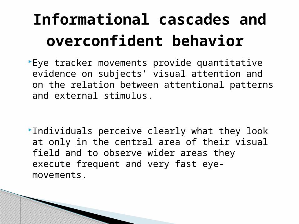
Both System 1 and System 2 are an evolutionary product. People heterogeneity as the result of individually specific patterns of interaction between the two systems

If eye movements and attention shifts are tightly tied, gaze direction could represent a signal of how automatic and immediate reactions (giving right or wrong information) to visual stimuli are modified or sustained by more conscious and rational processes of information collecting

Eye-movements and Systems 1/2

Informational cascade - model to describe and explain herding and imitative behavior focusing on the rational motivation for herding (Banerjee 1992, Bikhchandani et al. 1992)

Key assumptions

Other individuals’ action but not information is publicly observable 

private information is bounded in quality  agents have the same quality of private

information

Informational cascades

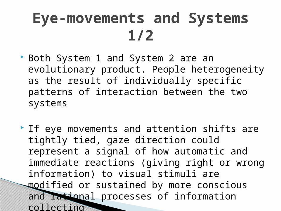
Consider two restaurants named "A" and "B" located next to one another

According to experts and food guides A is only slightly better than B (i.e. the prior probabilities are 51 percent for restaurant A being the better and 49 percent for restaurant B being better)

People arrive at the restaurants in sequence, observe the choices made by people before them and must decide where to eat

Apart from knowing the prior probabilities, each of these people also got a private signal which says either that A is better or that B is better (of course the signal could be wrong)

The restaurant example

Suppose that 99 of the 100 people have received private signals that B is better, but the one person whose signal favors A gets to choose first

Clearly, the first chooser will go to A. The second chooser will now know that the first chooser had a signal that favored A, while his or her own signal favors B 

Since the private signals are assumed to be of equal quality, they cancel out, and the rational choice is to decide by the prior probabilities and go to A

The restaurant example

The second person thus chooses A regardless of her signal

Her choice therefore provides no new information to the next person in line: the third person's situation is thus exactly the same as that of the second person, and she should make the same choice and so on 

Everyone ends up at restaurant A even if, given the aggregate information, it is practically certain that B is better (99 people over 100 have private signal that is the case)

This takes to develop a “wrong” information cascade, i.e. that is triggered by a small amount of original information followed by imitations

The restaurant example

A is chosen although almost all people receive private signal that B is better than A and there is no clear prior evidence that A is better than B (51% vs. 49%)

If the second person had been someone who always followed her own signal, the third person would have known that the second person's signal had favored B. The third person would then have chosen B, and so everybody else

The second person's decision to ignore her own information and imitate the first chooser inflicts a negative externality on the rest of the population

lf she had used her own information, her decision would have provided information to the rest of the population, which would have encouraged them to use their own information as well

What is wrong?

People have private information ("signals") and can also observe public information

Public information is a history of all the actions (not information) of predecessors

People are rational because they are assumed to update their prior probabilities by using Bayes’ rule to process the public and private information they possess

An individual herds on the public belief when his action is independent of his private signal

If all agents herd there is an informational cascade that may be both “wrong” or “right”

Model’s key features

The theory of informational cascades assumes that decision makers behave rationally in processing all the available information

Experimental evidence points out how subjects exhibit in the laboratory various cognitive biases in deciding if entering or not a cascade:

One third of the subjects exhibit a tendency to rely on the mere counting of signals (Anderson-Holt 1997)

Subjects’ overconfidence consistently explains the deviations from Bayes’ rule (Huck-Oechssler 2000, Nöth-Weber 2003, Spiwoks et al. 2008)

Heuristics and biases in cascades

Experimental setting

Two events - Square and Circle - may occur with equal probability.

For each session, 9 students were arranged in a pre-specified order and asked to predict the state with a monetary reward for a correct prediction

Each subject observes: an independent and private signal (Private Draw)

which has a 2/3 chance of indicating the correct event

the predictions (Previous Choices) made by the subjects choosing previously

Experimental Design

Private draw

?

2/3

1/3

2/3

1/3

HP: rational subjects process information according to Bayes’ rule and predict the event indicated as more probable by the combination of private signals and publicly known predictions

This implies that the choice of the first decision maker reveals the private signal he has drawn

  For example, if he chooses A, later decision makers

will infer that he has observed the signal a[Pr(a|A)=2/3 > Pr(a|B)=1/3]

Bayesian learning

If the second decision maker observes the same private signal a he will predict accordingly.

If she receives the other signal b, he will assign a 50% probability to the two events and both predictions will be equally rational.

If the second decision maker chooses A, the third decision maker will observe two previous choices of A. If her private signal is b, it will be rational to ignore this private information and to predict A as the previous choosers (information cascade).

 

Bayesian learning

If (a,b) indicates the numbers of signals a and b received or inferred, Bayes’ rule imposes: 

[Pr(a,b|A) Pr(A)] Pr (A|a,b) = ______________________________________________

[Pr(a,b|A) Pr(A) + Pr(a,b|B) Pr(B)]

In the example, the third decision maker observes two signals a inferred and receives one signal b received and the expression above gives:

(2/3)2(1/3)(1/2) Pr (A|a,b) = ______________________________________________________= 2/3 (2/3)2(1/3)(1/2) + (1/3)2(2/3)(1/2)   

Bayesian learning

Being signals balanced [Pr(A|a) = Pr(B|b) = 2/3], the difference between the number of signals a and b inferred or observed determines the more probable event.

In this simplified case, Bayes’ rule corresponds to a very simple and intuitive counting heuristic, which is easily computable by all subjects.

  In the example above, the third decision maker has to

count two previous choices over his/her only one private signal to determine her choice of A as rational 

 

Bayesian learning

Experiment 1

Session Treatment Participants (women + men)

1 (PD left - PC right) 9 (4 + 5) 2 (PD left - PC right) 9 (5 + 4) 3 (PD left - PC right) 9 (6 + 3) 4 (PC right - PD left) 9 (4 + 5) 5 (PC right - PD left) 9 (5 + 4) 6 (PC right - PD left) 9 (5 + 4) 7 (PD left - PC right) 9 (3 + 6) 8 (PD left - PC right) 9 (5 + 4) 9 (PD left - PC right) 9 (4 + 5)

Total 81 (41+40)

Participants: 81 Mean age: 22,4 Years

First screen (5 seconds)

2 sec

Private draw- PD (right)

Previous choice-PC (left)

Initial screen (2 seconds)

First screen (5 seconds)

Second screen (5 seconds)

First Fixations

Total number of fixations (Fixations = gazing at region of interest –ROI- for at least 200 milliseconds)

Relative time spent fixating ROI (relative time = time in a ROI divided by the total time spent on a task)

Sequence of last fixations

Experimental variables

BAYESIAN - the equal probability of the two states implies that the optimal Bayesian decision rule is to predict the state which obtains the greatest number of observed (Private draw) and inferred signal (Previous choices).

If subjects choose differently from what implied by Bayesian update: 

OVERCONFIDENT - if subject’s choice is equal to his Private draw

IRRATIONAL - if subject’s choice is not equal to his Private draw

Subjects’ types

Subjects’ types

Order of choice Bayesian Overconfident Irrational

1st 6 0 3 2nd 9 0 0 3rd 5 2 2 4th 6 2 1 5th 7 1 1 6th 6 2 1 7th 6 3 0 8th 6 3 0 9th 6 3 0

Total 57 16 8 Total (first chooser excluded) 51 16 5

Total allocation of attention

TABLE 5. TOTAL ALLOCATION OF ATTENTION (PERCENTAGE OF TOTAL TIME) PRIVATE

DRAW (PD) FORMER

CHOICES (FC) NO FIXATION TOTAL FORMER CHOICES/

N. OF FORMER

CHOICES BAYESIAN 26.9 63.0 10.1 100 22.4 OVERCONFIDENT 10.4 86.4 3.2 100 19.5 IRRATIONAL 47.1 39.9 13.0 100 22.6 TOTAL 25.6 65.3 9.1 100 21.8

TABLE 6. TOTAL ALLOCATION OF ATTENTION BY SCREEN SIDE (PERCENTAGE OF TOTAL TIME) PRIVATE DRAW FORMER CHOICES / N. OF FORMER

CHOICES LEFT SIDE RIGHT SIDE TOTAL LEFT SIDE RIGHT SIDE TOTAL

BAYESIAN 19.5 29.5 26.9 25.5 21.2 22.4 OVERCONFIDENT 9.2 10.9 10.4 16.8 20.7 19.5 IRRATIONAL 52.0 12.7 47.1 21.4 27.5 22.6 TOTAL 25.6 21.8

Only irrational subjects were significantly more inclined to look at

private draw (47.1%) than at former choices (22.6%).

First fixations

Private Draw Previous Choices

Latency offirst fixations

N. of first fixations

% N. of first fixations

% Averageduration

Bayesian 0.306 sec27

(13L+14R)

52.924

(13L+11R)

47.1 0.838 sec

Overconfident 0.412 sec 13 (6L+7R) 81.2 3 (1L+2R) 18.8 0.523 sec

Irrational 0.191 sec 3 (2L+1R) 60.0 2 (0L+2R) 40.0 0.835 sec

Total 0.321 sec43

(21L+22R)

46.825

(14L+15R)

53.2 0.775 sec• Overconfident subjects allocated their initial attention to private draw in 81% of the cases, and exhibited a longer average reaction time (0.412 sec.) and a shorter average duration of first fixation (0.523)

First fixations by side

TABLE 4. FIRST FIXATION BY SCREEN SIDES (FIRST CHOOSERS EXCLUDED)

PRIVATE DRAW (PD) FORMER CHOICES (FC)

LEFT RIGHT LEFT RIGHT

N. TOT. % N. TOT. % N. TOT. % N. TOT. %

BAYESIAN 8 14 57.1 20 30 66.6 16 38 42.1 6 16 37.5

OVERCONFIDENT 5 9 55.6 9 15 60.0 2 6 33.3 1 3 33.3

IRRATIONAL 1 1 100 2 3 66.6 2 4 50.0 0 3 0

TOTAL 14 24 58.3 31 48 64.6 21 48 43.7 8 24 33.3

No statistically significant difference between left and right orientation of the screen

was detected and the pattern of first fixations across subjects’ types

Likelihood to look at the chosen item

2.00

1.90

1.80

1.70

1.60

1.50

1.40

1.30

1.20

1.10

1.00

0.90

0.80

0.70

0.60

0.50

0.40

0.30

0.20

0.10

0.00

0

0.1

0.2

0.3

0.4

0.5

0.6

0.7

Time until decision (sec.)

Pro

ba

bili

y o

f lo

oki

ng

at t

he

ch

ose

n s

ign

al

No gaze cascade effect: observers gaze was not increasingly directed towards the chosen signal

Likelihood by types

Fig.2 Likelihood that subjects look at the chosen signal as a function of time until decision (by subjects' types)

0,62

0,64

0,66

0,68

0,7

0,72

0,74

0,76

0,78

Ba

yesi

an

i

00,020,040,060,080,10,120,140,160,180,2

Ove

rco

nfi

de

nt

Bayes

Overconf

Overconfident subjects allocate the first fixation (initial attention) toward private draw and take more time than others to decide if the private signal is on the right or the left of the screen.

Bayesian subjects allocate their initial attention to both kinds of information without exhibiting any particular bias

No evidence of the gaze cascade effect

Findings

In terms of the Dual Process theory, our findings support the hypothesis that automatic detection, as inferred from gaze direction, depends on cognitive biases.

The heuristic and automatic functioning of System 1 orients attention so as to confirm rather than to eventually correct these biases.

The controlled search attributable to System 2 does not significantly differ across subject types.

Interpretation

“Highly accessible impressions produced by System 1 control judgments and preferences, unless modified or overridden by the deliberate operations of System 2.” (Kahneman and Frederick 2002, p. 53)

Gaze participates actively in the process of choice under uncertainty

first fixation effect ⇒ orienting choice gaze cascade effect ⇒ reinforcing choice

Conclusions (1)

Heuristic processes of System 1 select the aspect of the task on which gaze direction is immediately focused

Analytic processes of System 2 derive inferences from the heuristically-formed representation through subsequent visual inspection

This dual account of visual attention orienting may explain the emergence of cognitive biases whenever relevant information is neglected at the heuristic stage.

Conclusions (2)

Voting by ballots and by feet

48

• Aim- is to provide experimental evidence on the Tiebout efficiency-enhancing property in a decentralized system of public goods provision

• Object - a test of the Tiebout model in order to assess if

decentralization and local sorting produces efficiency gains

• Key finding – we show that the model fails because residents are different, not only in their preferences on local public goods, but also because voting and moving are not equally shared.

The Tiebout Model

Tiebout’s (1956) model shows that if a sufficient number of local communities exists to accommodate different types of preferences, individuals could move to that community whose local governments best satisfies his set of preferences (pattern of expenditures and taxes).

Quoting Oates (1969) “Tiebout’s world is one in which the consumer “shops” among different communities offering varying packages of local public services and selects as a residence the community which offers the tax-expenditure program best suited to his tastes”.

The Tiebout Model

This is the so called voting by feet

if households are free to move, people effectively sort themselves into groups that are homogeneous with respect to their demands for local services.

More recently Since 1956, there is a wealth of literature surrounding

the Tiebout hypothesis, both from an empirical and a theoretical point of view.

Rodhe and Strumpf (American Economic Review, 2003) argue that long–run trends in geographical segregation are inconsistent with choice model where residential choices depends solely on local public goods

More precisely they demonstrate that the secular decline in the mobility costs is not matched with an increase in the heterogeneity in local public policies

Rhode and Stumpf (AER, 2003)

Some example of mobility costs historical data - CAR: in 1903 to drive a car cost 143,8 cents/mile

in 1998 dollars, while in 1998 54,9 cents;- TRAIN: a passenger mile cost 37,4 cents in 1895

and 13,4 cents in 1995;- AIR: a passenger mile cost 108 cents in 1929 vs.

13,7 cents in 1995;- 3 minute of transcontinental call in January

1915 cost 20,70$ in current dollars, which was almost 314$ in 1998 dollars.

Rhode and Stumpf (AER, 2003)

Data on a sample of US municipalities (1870-1990), all Boston-area municipalities (1870-1990) and all US counties (1850-1990) show that municipal per capita taxes, school district per capita taxes, total spending, protection spending etc. incomes and racial composition are now less differentiate across local communities than in the past.

Rhode and Stumpf (AER, 2003)

They explain this result as follows1. growing federal role in providing public

services2. zoning policies are more and more popular

after the war, avoiding the poor-chasing-the-rich phenomenon

3. growing local government competition (to have the same category of residents: the richer !)

Our explanationIn our paper we test a fourth cause of the phenomenon observed.

We show that the Tiebout model may fail not only because residents have heterogeneous preferences on local public goods, but also because voting and moving are not equally shared.

The experimental design• 2 treatments x 3 sessions• 10 rounds for each session• In each session 15 subjects (undergraduate

students) are randomly allocated in 5 communities • Each community is allowed to provide only one

public good• The four suits of cards (clubs, diamonds, hearts,

spades) represent different types of public goods• Playing cards randomly assigned to each subject

for the whole experiment• The number over the cards determines subject’s

preferences over public goods

The experimental designThe individual welfare given by public good provision is the difference between individual benefit and individual cost.

The individual benefit given by public good provision is the minimum between the community provision level and the sum of cards of that public good (suit) possessed.

The individual cost is equal to the community production cost, that is the quantity produced (Hp. constant and unitary costs) divided by the number of community members (Hp. community total cost is shared equally among the members of the community).

i typeof cards of sum i, typeof levelprovision minB

Two treatments

In each community there is a subject (the dictator) who decides before each of the 10 rounds the type and the amount of the public good to produce

The other community members can only move or not move and are informed of the type and the amount of goods produced by all the communities before deciding

In each of the 10 rounds each community decides by majority vote the type and the amount of the public good to produce

All subjects can move or not move and are informed of the good produced by all the communities in the previous period

Dictator treatmentDemocracy treatment

1 2 3 4 5 6 7 8 9 100

10

20

30

40

50

60

Session 1

1 2 3 4 5 6 7 8 9 100.00

10.00

20.00

30.00

40.00

50.00

60.00

Session 2

1 2 3 4 5 6 7 8 9 100.00

10.00

20.00

30.00

40.00

50.00

60.00Session 3

Democracy treatment Dictator treatment

Total welfare

Average per capita cost

1 2 3 4 5 6 7 8 9 100

1

2

3

4

5

6

Session 1

1 2 3 4 5 6 7 8 9 100.00

0.50

1.00

1.50

2.00

2.50

3.00

3.50

4.00

4.50

Session 2

1 2 3 4 5 6 7 8 9 100.00

0.50

1.00

1.50

2.00

2.50

3.00

3.50

4.00

Session 3

Democracy treatment Dictator treatment

Average produced quantity

1 2 3 4 5 6 7 8 9 10012345678

Session 1

1 2 3 4 5 6 7 8 9 100.00

1.00

2.00

3.00

4.00

5.00

6.00

7.00

8.00

Session 2

1 2 3 4 5 6 7 8 9 100.00

1.00

2.00

3.00

4.00

5.00

6.00

7.00

8.00

Session 3

Democracy treatment Dictator treatment

Data analysis Total welfare is higher in the democracy treatment

i.e. voting by feet increases efficiency if voting by ballot is equally shared

Average cost per capita is higher in the dictator treatment

In the democracy treatment cost per capita tends to increase in the first part of the session, but decreases after the 5th-6th rounds

Quantity produced does not statistically differentiate across treatments

Statistical analysis

Democracy Dictator Democracy Dictator Democracy DictatorVARIABLES deltaW deltaW deltaW deltaW deltaW deltaW

Nr of moving in 10 rounds 1.019*** 0.295** 0.278*** 0.380*** 0.325*** -0.480***(0.098) (0.142) (0.103) (0.088) (0.070) (0.090)

Nr. of Rounds in wich a person with an opposite SC is meet -0.439*** -0.168 -3.320*** 2.440*** -0.813*** 0.447***

(0.063) (0.120) (0.593) (0.275) (0.242) (0.084)Nr. of Rounds in wich at least two people with an opposite SC are meet -0.576*** -0.091 -0.096 -0.419* -0.729*** 0.511***

(0.045) (0.119) (0.113) (0.229) (0.099) (0.127)

Moving/non moving decisions taken rightly 1.106*** -1.003*** 4.795*** -0.481*** -0.544*** 0.076(0.147) (0.289) (0.275) (0.148) (0.172) (0.364)

Community in which the individual move is chosen rightly -0.291*** 1.625*** -5.218*** 0.577*** 0.783*** 0.060

(0.102) (0.241) (0.317) (0.158) (0.115) (0.165)Constant -4.460*** -3.230*** 4.991*** -1.552 2.729** 0.615

(0.765) (1.223) (0.806) (1.023) (1.254) (1.960)

Observations 150 100 150 100 150 100R-squared 0.764 0.685 0.787 0.667 0.762 0.444Standard errors in parentheses

*** p<0.01, ** p<0.05, * p<0.1

Session 1 Session 2 Session 3OLS -Welfare difference between 10th-1th round

Statistical results

Positive correlation between the number of moving individuals and the increase of individual welfare in all the sessions of the democracy treatment, and in two out of three session in the dictator treatment

In the democratic treatment, the welfare increase is negatively related with the number of rounds in which each individual met a person with a SRCC* of the opposite sign, while in the dictator treatment this variable is not significantly correlated with welfare.

*we evaluate heterogeneity in preferences within communities by calculating Spearman's Rank Correlation Coefficients between each one experimental subject and all the others

Interpretations

In the democratic treatment the welfare increase is positively related with the right decision of moving/non moving

In the dictator treatment the sign of the correlation between welfare increase and the decision of moving/non moving depends on the chosen community

Voting by feet enhances welfare, by reducing heterogeneity among members of a community, only if all that people has the right to vote.

Analysis of moving/non moving

Democracy Dictator Democracy Dictator Democracy DictatorVARIABLES move move move move move move

Individual loss in the previous round(dummy) 1.972*** 2.160*** 1.174*** 2.004*** 1.642***(0.374) (0.550) (0.268) (0.422) (0.378)

Decision taken in the f irst f ive rounds(dummy) 0.564** 0.889*** 0.529* 1.398*** -0.229(0.263) (0.313) (0.276) (0.388) (0.310)

Presence of at least one person w ith a SC w ith the opposite sign 1.137*** -0.540 0.425 1.063***

(0.308) (0.418) (0.388) (0.352)Presence of at least tw o people w ith a SC w ith the opposite sign 0.744** 0.033 -0.596 0.010

(0.336) (0.398) (0.651) (0.483)Different individual vote on the type of good produced(dummy) 1.278***

(0.487)Different individual vote on the quantity of good produced(dummy) 0.623**

(0.243)Constant -1.700*** -1.184*** -1.277*** -0.698*** -2.277*** -0.639***

(0.265) (0.251) (0.205) (0.197) (0.368) (0.219)

Observations 150 100 150 100 150 100Standard errors in parentheses

*** p<0.01, ** p<0.05, * p<0.1

Session 1 Session 2 Session 3

Probit Moving-Non Moving

Moving decisions

1. Individual loss in previous rounds is always significantly correlated with the decision to move in both treatments

2. Moving decisions are taken more often in the first five rounds

3. In the democracy treatment the decision to move is mainly influenced by community heterogeneity or by the discrepancy between vote and public good produced

Conclusions

Total welfare is always higher in democracy, i.e. voting by feet increases efficiency if voting by ballot is equally shared among residents

Under democracy the increase of individual welfare is positively related to the number of moving decisions

The better performance of the democratic process over the dictatorship depends on the decreaseof the average public good costs per capita

Conclusions

In democracy, the welfare increase is negatively related with the heterogeneity of people in each community, while in the dictator design this variable is not significant

In the dictator design the increase in welfare is positively related with a right decision on moving/non moving only if the community is correctly chosen, while in the democracy design there is a positive coefficient if the moving/non moving decision is rightly taken.

Aim: to extend previous experimental evidence on travel mode choice by providing subject not only with information acquired through personal experience, but also with actual travel times of the alternative non chosen travel modes

Key Findings: subjects exhibit a marked preference for cars are inclined to confirm their first choices update imperfectly expectations on travel times

Travel mode choice and transportation policy

Experimental literature on travel mode choice relies on studies on route choice

Common object: coordination games, i.e. the payoff each traveler can achieve is conditional on her/his ability to diverge from or to converge with other travelers’ choices

Selten et al. (2007), Ziegelmeyer et al. (2008), Razzolini-Dutta (2009) provide laboratory evidence that choices between route A and route B generate Nash equilibria

Background literature

Evidence from the field that these learning processes are affected by cognitive biases (Kareev et al. 1997, Verplanken–Aarts 1999)

To provide travelers with more accurate information on actual travel times does not necessarily increase their propensity to minimize travel costs (Avineri-Prashker 2006)

Information is better processed when travelers lack long-term experience on travel time distribution (Ben Elia–Erev-Shiftan 2008)

Background literature

Cars are generally perceived as travel means giving people the sensation of freedom and independence

The costs associated to car use are undervalued because they not paid contextually with car use

Pollution or social costs due to car accidents are often neglected and not easily computable

These factors explain the presence of a general propensity to use private cars and of a psychological resistance to reduce it (Van Vugt et al. 1995, Tertoolen et al. 1998, Bamberg et al. 2003)

Background literature

62 undergraduate students (31 women and 31 men) from the University of Firenze

Computerized experiment

Between subject

Each session lasted approximately an hour

Average earnings 18.4 euro

The design

1) Choice between car or metroMetro travel costs are fixed, while car costs are uncertain and determined by the joint effect of casual events and traffic congestion

2) Choice between car or busCar and bus are both uncertain and determined by the combination of casual events and traffic congestion.

Travelers’ utility only depends on travel times, which are converted in monetary costs. After each choice, subjects are informed of actual times of both available modes, but not of the probability distributions determining casual events

The design

The design

Table 2 Experimental parameters made known to subjects

Treatment Car Expected Time Travel (in minutes)

Car Fixed Cost

Metro / Bus Expected Time

Travel

Metro / Bus Fixed Cost

Metro vs. Car 25 1.5 30 1.0

Bus 1.0 vs. Car 27 1.5 32 1.0

Bus 0.8 vs. Car 27 1.5 32 0.8

Metro Car treatment- the expected total costs of car and metro were equivalent if the share of car users was not greater than 55%;

Bus 1.0 Car treatment - the expected total costs of car and bus were equivalent if the share of car users was not greater than 55%;

Bus 0.8 Car treatment- the expected total cost of the bus was 20% lower than car expected total costs if the share of car users was not greater than 55%.

The design

Results – Preference for CarsTable 8 Proportion of car choices by treatment (each five periods)

Period Metro Bus 1.0 Bus 0.8 1 0.70 0.60 0.59 5 0.67 0.67 0.35

10 0.60 0.47 0.35 15 0.57 0.67 0.47 20 0.57 0.53 0.53 25 0.77 0.53 0.41 30 0.67 0.73 0.71 35 0.70 0.60 0.71 40 0.60 0.53 0.53 45 0.67 0.60 0.53 50 0.73 0.53 0.53

Total 0.68 0.58 0.50

Results– Preference for cars

Results – Preference for cars

Results – Preference for cars

Results – Preference for cars

Results – First Choice Effect

Results – First Choice Effect

Results– Travel Mode Stickiness

The first choice effect decreases the propensity to change travel mode

Only 28.6% of the subjects in the metro treatment and 39% of the subjects in the bus treatments change more than 20 times over 50 periods.

On average, subjects change mode 17.7 times in the metro treatment and 18.0 times in the bus treatments

Travel mode choice is significantly affected by heuristics and biases that lead to robust deviations from rational behaviour

Travelers choose modes using behavioural rules that do not necessarily involve the minimization of total travel costs.

Subjects show a marked preference for cars, are inclined to confirm their first choice and exhibit a low propensity to change travel mode.

86

Conclusions

In repeated travel mode choice, available information is not properly processed, cognitive efforts are generally low and rational calculation play a limited role

The habit of using cars should be assumed to be relatively resistant, to the effect of economic incentives

Little progress can be expected by asking travelers to voluntarily reduce the use of a car or even by subsidizing public transport costs

87

Conclusions

One of the basic tenets of laboratory methodology is that the use of non-professional subjects and monetary incentives allows making subjects’ innate characteristics largely irrelevant

In our experiment, it is as if subjects take into the lab the preferences applied to real choices and stick to them with high probability

This inclination to prefer cars tends to override the incentives effect

Labels give subjects clues to become less and not more rational

Back to Methodology

In our experiment, subjects’ behavior depends more on prior learning outside the laboratory than on expected gains in the laboratory

Labels have the power to increase external validity with a minimal sacrifice of the internal validity

To test learning and cognitive models, it is necessary to remind and to evoke contexts which may activate emotions, association, similarities in the laboratory

The power of labels

Tramhttp://www.youtube.com/watch?v=H1XrL_U38-c

Metrohttp://www.youtube.com/watch?v=dYmsmWqCV0A

Carhttp://www.youtube.com/watch?NR=1&v=Sk-WlKTtExA

Progetto ALBOhttp://www.progettoalbo.it/images/video/trailer.mp4

LAVREB Laboratory of Virtual reality and Economic Behaviorhttp://www.lavreb.unisi.it/

Some examples