PHYSICAL REVIEW A 81, 052324 (2010)

Phase transitions and metastability in the distribution of the bipartite entanglementof a large quantum system

A. De Pasquale,1,2,3 P. Facchi,2,4 G. Parisi,5,6 S. Pascazio,1,2 and A. Scardicchio7,8

1Dipartimento di Fisica, Universita di Bari, I-70126 Bari, Italy2INFN, Sezione di Bari, I-70126 Bari, Italy

3MECENAS, Universita Federico II di Napoli, Via Mezzocannone 8, I-80134 Napoli, Italy4Dipartimento di Matematica, Universita di Bari, I-70125 Bari, Italy

5Dipartimento di Fisica, Universita di Roma “La Sapienza”, Piazzale Aldo Moro 2, I-00185 Roma, Italy6Centre for Statistical Mechanics and Complexity (SMC), CNR-INFM, I-00185 Roma, Italy

INFN Sezione di Roma, I-00185 Roma, Italy7Abdus Salam International Center for Theoretical Physics, Strada Costiera 11, I-34014 Trieste, Italy

8INFN, Sezione di Trieste, I-34014 Trieste, Italy(Received 13 January 2010; published 19 May 2010)

We study the distribution of the Schmidt coefficients of the reduced density matrix of a quantum system ina pure state. By applying general methods of statistical mechanics, we introduce a fictitious temperature and apartition function and translate the problem in terms of the distribution of the eigenvalues of random matrices. Weinvestigate the appearance of two phase transitions, one at a positive temperature, associated with very entangledstates, and one at a negative temperature, signaling the appearance of a significant factorization in the many-bodywave function. We also focus on the presence of metastable states (related to two-dimensional quantum gravity)and study the finite size corrections to the saddle point solution.

DOI: 10.1103/PhysRevA.81.052324 PACS number(s): 03.67.Mn, 03.65.Ud, 68.35.Rh

I. INTRODUCTION

Entanglement is an important resource in quantum infor-mation processing and quantum enabled technologies [1,2].Besides its important applications in relatively simple systems,that can be described in terms of a few effective quantumvariables, it is also widely investigated in many-body systems[3,4], where the bipartite entanglement can be given asatisfactory quantitative definition in terms of entropy and itslinearized versions, such as purity [5,6]. The characterizationof the global features of entanglement is more involved,unveiling in general different features of the many-body wavefunction [7,8], and it is becoming clear that the multipartiteentanglement of a large system cannot be fully characterizedin terms of a single (or a few) measure(s).

Entanglement measures the nonclassical correlations be-tween the different components of a quantum system andunearths different characteristics of its many-body wave func-tion. When the quantum system is large, it becomes thereforeinteresting to scrutinize the features of the distribution of somebipartite entanglement measure, such as the purity or the VonNeumann entropy. Besides being of interest for applications,this is an interesting problem in statistical mechanics. In [9]we tackled this problem by studying a random matrix modelthat describes the statistical properties of the eigenvalues ofthe reduced density matrix of a subsystem A of dimension N

(the complementary subsystem B having the same dimensionas A). In the limit of large system dimension N , we introduceda partition function for the canonical ensemble as a function ofa fictitious temperature. The role of energy is played by purity:different temperatures correspond to different entanglement.The most important result of our analysis was the proof that thedifferent regions of entanglement, corresponding to differentranges of the fictitious temperature, are separated by phasetransitions.

One puzzle was left open in that paper: in the region ofnegative temperatures our solution suddenly ceased to existat a critical βg where the average purity of subsytem A wasπAB = 9/4N [a phenomenon quite common in random matrixtheory, as this critical point corresponds to tesselations ofrandom surfaces, or two-dimensional (2-D) quantum gravity].As the partition function exists for all β ∈ R, the region offactorizable states, where πAB = O(1), was not covered.

We will show in this paper that the solution in [9] becomesmetastable for any β < 0 (in the scaling of [9]) and a newstable solution appears which interpolates smoothly fromπAB = 2/N to πAB = 1 as β goes from 0 to −∞. Moreover,we will also study the metastable solution that is born at β = 0and follow it through the region 0 > β > −∞.

This paper is organized as follows. In Sec. II we introducethe notation and set the bases of the statistical mechanicalapproach to the problem. In Sec. III we study positivetemperatures, where at very low temperatures we find veryentangled states. Negative temperatures are investigated inSec. IV, where it is shown that two branches exist, a stableone associated to a partial factorization of the many-body wavefunction, and a metastable one which contains the 2D-quantumgravity point. The finite size corrections are investigated inSec. V. We discuss the implications of our results for quantuminformation in Sec. VI and we conclude in Sec. VII bysummarizing our findings and discussing them in terms offuture perspectives.

II. A STATISTICAL APPROACH TO THE STUDYOF BIPARTITE ENTANGLEMENT

We start off by describing a statistical approach to the studyof bipartite entanglement for large quantum systems. We willtackle this problem by introducing a partition function [9].

1050-2947/2010/81(5)/052324(20) 052324-1 ©2010 The American Physical Society

A. DE PASQUALE et al. PHYSICAL REVIEW A 81, 052324 (2010)

Consider a bipartite system, composed of two subsystemsA and B. The total system lives in the tensor product Hilbertspace H = HA ⊗ HB , with dimHA = N � dimHB = M .We assume that the system is in a pure state |ψ〉 ∈ H. Thereduced density matrix of subsystem A reads

ρA = TrB |ψ〉〈ψ |, (1)

and is a Hermitian, positive, unit-trace N × N matrix. A goodmeasure of the entanglement between the two subsystems isgiven by the purity,

πAB = TrAρ2A = TrBρ2

B =N∑

j=1

λ2j ∈ [1/N,1], (2)

whose minimum is attained when all the eigenvalues λj areequal to 1/N (completely mixed state and maximal entan-glement between the two bipartitions), while its maximum(attained when one eigenvalue is 1 and all others are 0) detectsa factorized state (no entanglement).

In order to study the statistics of bipartite entanglementfor pure quantum states, we consider typical vector states |ψ〉[10,11], sampled according to the unique, unitarily invariantmeasure. The significance of this measure can be understoodin the following way: consider a reference state vector |ψ0〉and a unitary transformation |ψ〉 = U |ψ0〉. In the least set ofassumptions on U , the measure is chosen in a unique way,being the only left- and right-invariant Haar (probability)measure of the unitary group U (N2). The final state |ψ〉will hence be distributed according to the measure mentionedabove (independently of |ψ0〉). Other distributions can alsobe considered but they encode additional information on thesystem (in this sense, Haar is the most “neutral”). Thesealternative distributions could be treated in our approach byconstraining the system by means of Lagrange multipliers(notice the analogy with the maximum entropy argument inclassical statistical mechanics). For an approximate realizationof this unique measure by means of short quantum circuits see[12], where it is proved that one can extract Haar-distributedrandom states by applying only a polynomial number ofrandom gates.

By tracing over subsystem B, this measure induces thefollowing measure over the space of Hermitian, positivematrices of unit trace [10,11],

dµ(ρA) = DρA(det ρA)M−Nδ(1 − TrρA),

= dNλ∏i<j

(λi − λj )2∏

�

ληN

� δ

(1 −

∑k

λk

), (3)

where λk are the (positive) eigenvalues of ρA (Schmidtcoefficients), we dropped the volume of the U (N ) group(which is irrelevant for our purposes) and ηN ≡ M − N isthe difference between the dimensions of the Hilbert spacesHA and HB . In order to study the statistical behavior of a largebipartite quantum system we introduce a partition functionfrom which all the thermodynamic quantities, for example,the entropy or the free energy, can be computed:

ZAB =∫

dµ(ρA) exp(−βNαπAB), (4)

where α is a positive integer (either 2 or 3, as we shall see)and β a fictitious temperature “selecting” different regions ofentanglement. The value of α needs to be chosen in order toyield the correct thermodynamic limit as

Nα〈πAB〉 = O(N2), (5)

since N2 is the number of degrees of freedom of the matrixρA. Around the maximally entangled states (for β > 0 [9])we have 〈πAB〉 = O(1/N) so α = 3, while around separablestates (for β < 0) we have 〈πAB〉 = O(1) and hence α = 2.In the following we will assume η = 0, since this does notchange the qualitative picture (the extension to η �= 0 beingstraightforward but computationally cumbersome).

Since the purity depends only on the eigenvalues of ρA thepartition function reads

ZAB =∫

λi�0dNλ

∏i<j

(λi − λj )2δ

(1 −

N∑i=1

λi

)e−βNα

∑i λ2

i ,

(6)

which by introducing a Lagrange multiplier for the deltafunction yields

ZAB = N2∫ ∞

−∞

dξ

2π

∫λi�0

dNλ

× eiN2ξ (1−∑i λi )−βNα∑

i λ2i +2

∑i<j ln |λi−λj |. (7)

A physical interpretation of the exponent in the integrandof the partition function can be given as follows [13]: theeigenvalues of ρA can be interpreted as a gas of interactingpoint charges (Coulomb gas) at positions λi’s, on the positivehalf-line and with a quadratic potential. The solution of theseintegrals is known (as Selberg’s integral) for the case in whichthe integration limits are −∞ < λi < +∞ [13].

The constraint of the positivity of the eigenvalues makes thecomputation of this integral far more complicated. Althoughan exact solution for finite N is unlikely to be found1 (butsee [9,14] for the first few moments), the problem arisingfrom the constraint on the positivity of the eigenvalues canbe overcome in the large N limit, as we will look for thestationary point of the exponent with respect to both the λ’sand ξ . In particular, the contour of integration for ξ lies on thereal axis, but we will soon see that the saddle point for ξ lieson the imaginary ξ axis. It is then understood that the contourneeds to be deformed to pass by this point parallel to the lineof steepest descent. For the saddle point we need to find theminimum of the free energy:

βF = βNα∑

i

λ2i − 2

∑i<j

ln |λi−λj | − iN2ξ

(1 −

∑i

λi

).

(8)

1An exact solution can always be found by means of the orthogonalpolynomials method, but the expressions for ZAB grow enormouslyin complexity with increasing N .

052324-2

PHASE TRANSITIONS AND METASTABILITY IN THE . . . PHYSICAL REVIEW A 81, 052324 (2010)

By varying F we find the saddle point equations,

−2βNαλi + 2∑j �=i

1

λi − λj

− iN2ξ = 0, (9)

∑i

λi = 1. (10)

In the following sections we will separately analyze the rangeof positive and negative temperatures, and unveil the presenceof two phase transitions for the system, a second-order one ata positive critical β and a first-order one at a negativecritical β.

A. The global picture

Before proceeding to a formal analysis of the phasetransitions, it is convenient to give a qualitative picture ofthe behavior of the Schmidt coefficients as the temperature ischanged. As the inverse temperature is decreased, the densitymatrix of subsystem A changes as follows. As β → +∞all eigenvalues are = 1/N (maximally mixed state). As β

decreases, we encounter two phase transitions: one at a positivecritical value β+ and one at a negative critical value β−, bothcritical values being to be determined. For β > β+ all eigen-values remain O(1/N ), their distribution being characterized,as we shall see, by the Wigner semicircle law. After the firstphase transition, for β+ > β > β−, the eigenvalues, all alwaysO(1/N ), follow the Wishart distribution, divergent at theorigin. Finally, after the second phase transition, for β < β−,one eigenvalue becomes O(1), “evaporating” from the “sea”of eigenvalues O(1/N ): this is a signature of the emergence offactorization in the many-body wave function, the eigenvalueO(1) being associated with a significant separability betweensubsystems A and B. For β → −∞ the many-body wavefunction is fully factorized. Pictorially, the typical eigenvaluesvector evolves starting from β = +∞ to β = −∞ as(

1

N,

1

N, . . . ,

1

N

)︸ ︷︷ ︸

β→+∞

−→(O

(1

N

), . . . ,O

(1

N

))︸ ︷︷ ︸

+∞>β>β+

−→(O

(1

N

),O

(1

N

), . . . ,0, . . . ,0

)︸ ︷︷ ︸

β+>β>β−

−→(O(1),O

(1

N

), . . . ,0, . . . ,0

)︸ ︷︷ ︸

β−>β>−∞−→ (1,0, . . . ,0)︸ ︷︷ ︸

β→−∞, (11)

where the zeros in the second and third lines mean anaccumulation of points around the origin, and we will findthat [in the scaling of β given by α = 3 in Eq. (5)], β+ = 2and β− = −2.455/N .

III. POSITIVE TEMPERATURES: TOWARD MAXIMALLYENTANGLED STATES

In this section we will consider the range of positivetemperatures: 0 < β < +∞; in particular we will study the

occurrence of a second-order phase transition at β = 2 [9]. Wewill use a more general method, that will enable us to find allsolutions and can be easily extended to negative temperatures.

From the expression of the partition function one can easilyinfer that when β → +∞ the typical states belonging to thisdistribution are maximally entangled states and correspond tothe case λi = 1/N , ∀i ∈ {1, . . . N}. It then follows that for thisrange of temperatures the right scaling exponent in (4) and (5)is α = 3.

In order to estimate the thermodynamic quantities of thesystem we solve the saddle point Eqs. (9) and (10) in thecontinuous limit, by introducing the natural scaling,

λi = 1

Nλ(ti), 0 < ti = i

N� 1. (12)

In the limit N → ∞, Eq. (9) becomes

−βλ + P

∫ ∞

0dλ′ ρ(λ′)

λ − λ′ − iξ

2= 0, (13)

which is a singular Fredholm equation of the first kind, knownas the Tricomi equation [15]. The function

ρ(λ) =∫ 1

0dt δ(λ − λ(t)), (14)

is the density of eigenvalues we want to determine. A similarequation, restricted at β = 0, was studied by Page [11].

According to the Tricomi theorem [11,15], the solutionof the integral Eq. (13) lies in a compact interval [a,b],(0 � a � b). Let us set

m = a + b

2, δ = b − a

2, 0 � δ � m. (15)

We map the interval [a,b] into the interval [−1,1] byintroducing the following change of variables:

λ = m + xδ, φ(x) = ρ(λ)δ. (16)

We get

1

πP

∫ 1

−1

φ(y)

y − xdy = g(x), (17)

with

g(x) = − 1

π

(iξ

δ

2+ βδm + βδ2x

), (18)

whose normalized solution (∫

φ dx = 1) is

φ(x) = − 1

πP

∫ 1

−1

√1 − y2

1 − x2

g(y)

y − xdy + 1

π√

1 − x2. (19)

By using the constraint (10), that is∫ 1

−1λ φ(x) dx = 1, (20)

we can fix the Lagrange multiplier to obtain

φ(x) = 1

π√

1 − x2

[1 + βδ2

2+ 2(1 − m)

δx − βδ2x2

].

(21)

The physical solutions must have a density φ(x) that isnonnegative for all x ∈ (−1,1). Let us look at the points where

052324-3

A. DE PASQUALE et al. PHYSICAL REVIEW A 81, 052324 (2010)

β = 0

0.51

23m

δ0 0.5 1 1.5 2

0

0.5

1

1.5

2

FIG. 1. (Color online) Solution domain for different values oftemperature: for each value of β (indicated) the relative full lineencloses the region of the parameter space such that the eigenvaluedensity is positive. The line m = δ corresponds to the positiveeigenvalues condition.

the density vanishes, φ(x) = 0. From (21) one gets

x± = 1

βδ2

(1 − m

δ±

√�

), (22)

where

� =(

1 − m

δ

)2

+ βδ2

(1 + βδ2

2

). (23)

For β � 0 one gets that � � 0 for every m and δ, and φ(x) �0 for x ∈ [x−,x+]. The level curves x± = ±1 are given bym = ±

1 (δ,β), where

±1 (δ,β) = 1 ± δ

2

(1 − βδ2

2

). (24)

They are symmetric with respect to the line m = 1 and intersectat δ = 0 and at δ = √

2/β. Therefore, the condition (−1,1) ⊂[x1,x2] implies that the points (δ,m) should be restricted to a(possibly cut) “eye-shaped” domain given by

max{δ, −1 (δ,β)} � m � +

1 (δ,β), (25)

[recall the constraint m � δ in (15) that expresses the positivityof eigenvalues]. The right corner of the eye is at

(δ,m) =(√

2

β,1

), (26)

and belongs to the boundary as long as β � 2. For β < 2the eye is cut by the line m = δ; see Fig. 1. Let us remarkthat all points inside the region correspond to solutions ofthe saddle point equations. In other words we have a two-parameter continuous family of solutions. We will look at theeigenvalue density that minimizes the free energy density ofthe system. From Eqs. (8) and (10) with α = 3 by applyingthe scaling (12) we get

fN = F

N2= 1

N

∑i

λ(ti)2 − 2

N2β

∑i<j

ln |λ(ti) − λ(tj )|

+ 2

N2β

∑i<j

ln N

= u − 1

βs + ln N + O

(ln N

N

)

= f + ln N + O

(ln N

N

). (27)

Here,

f = limN→∞

(fN − 1

βln N

)(28)

is the free energy density in the thermodynamic limit, whichreads

βf = βu − s, (29)

in terms of the internal energy density u and the entropydensity s,

u =∫ 1

−1λ2φ(x)dx,

(30)

s =∫ 1

−1dx

∫ 1

−1dy φ(x)φ(y) ln(δ|x − y|).

In order to compute the entropy density one integrates theTricomi Eq. (17) and obtains∫ 1

−1φ(x)dx

∫ 1

−1φ(y)dy ln |y − x|

=∫ 1

−1dxφ(x) ln(x + 1) − π

∫ 1

−1dxφ(x)

∫ x

−1g(y)dy. (31)

We get

u(δ,m,β) = 1 − (1 − m)2 + δ2

2− βδ4

8, (32)

s(δ,m,β) = −2(1 − m)2

δ2− β2δ4

16+ ln

δ

2, (33)

and thus

βf (δ,m,β) = β − β(1 − m)2 + 2(1 − m)2

δ2+ βδ2

2

− β2δ4

16− ln

δ

2. (34)

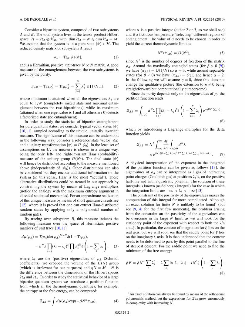
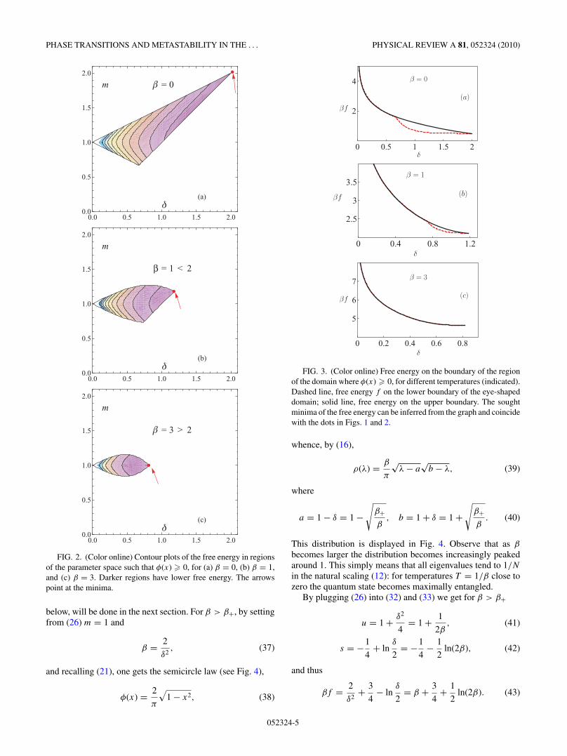
The contour plots of the free energy are shown in Fig. 2.Note that f , as well as u and s, is symmetric with respectto the line m = 1. This Z2 symmetry will play a major rolein the following. The only stationary point (a saddle point)of the free energy density f is at the right corner of the eye(26); see Figs. 1 and 2. Thus, the absolute minimum is on theboundary.

For β � β+, where

β+ = 2, (35)

the point (26) is also the absolute minimum, whereas for 0 <

β < β+ the absolute minimum is at the right upper corner ofthe allowed region, δ = +

1 (δ,β), namely at

m = δ, with βδ3

4+ δ

2− 1 = 0. (36)

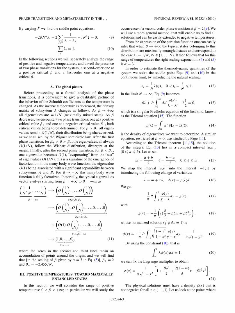
See the dots in Figs. 1 and 2. The behavior of the free energyat the boundaries of the allowed domain is shown in Fig. 3 fordifferent temperatures.

We will study the behavior of our system starting from highvalues of β, that is, low values of internal energy u (purity).The analysis of lower values of β, down to β = 0 and even

052324-4

PHASE TRANSITIONS AND METASTABILITY IN THE . . . PHYSICAL REVIEW A 81, 052324 (2010)

m

δ

β = 0

(a)

0.0 0.5 1.0 1.5 2.00.0

0.5

1.0

1.5

2.0

m

δ

β = 1 < 2

(b)

0.0 0.5 1.0 1.5 2.00.0

0.5

1.0

1.5

2.0

m

δ

β = 3 > 2

(c)

0.0 0.5 1.0 1.5 2.00.0

0.5

1.0

1.5

2.0

FIG. 2. (Color online) Contour plots of the free energy in regionsof the parameter space such that φ(x) � 0, for (a) β = 0, (b) β = 1,and (c) β = 3. Darker regions have lower free energy. The arrowspoint at the minima.

below, will be done in the next section. For β > β+, by settingfrom (26) m = 1 and

β = 2

δ2, (37)

and recalling (21), one gets the semicircle law (see Fig. 4),

φ(x) = 2

π

√1 − x2, (38)

βf

δ

β = 0

(a)

0 0.5 1 1.5 2

2

4

βf

δ

β = 1

(b)

0 0.4 0.8 1.2

2.5

3

3.5

βf

δ

β = 3

(c)

0 0.2 0.4 0.6 0.8

5

6

7

FIG. 3. (Color online) Free energy on the boundary of the regionof the domain where φ(x) � 0, for different temperatures (indicated).Dashed line, free energy f on the lower boundary of the eye-shapeddomain; solid line, free energy on the upper boundary. The soughtminima of the free energy can be inferred from the graph and coincidewith the dots in Figs. 1 and 2.

whence, by (16),

ρ(λ) = β

π

√λ − a

√b − λ, (39)

where

a = 1 − δ = 1 −√

β+β

, b = 1 + δ = 1 +√

β+β

. (40)

This distribution is displayed in Fig. 4. Observe that as β

becomes larger the distribution becomes increasingly peakedaround 1. This simply means that all eigenvalues tend to 1/N

in the natural scaling (12): for temperatures T = 1/β close tozero the quantum state becomes maximally entangled.

By plugging (26) into (32) and (33) we get for β > β+

u = 1 + δ2

4= 1 + 1

2β, (41)

s = −1

4+ ln

δ

2= −1

4− 1

2ln(2β), (42)

and thus

βf = 2

δ2+ 3

4− ln

δ

2= β + 3

4+ 1

2ln(2β). (43)

052324-5

A. DE PASQUALE et al. PHYSICAL REVIEW A 81, 052324 (2010)

φ(x

)

x

β ≥ β+

1 0.5 0 0.5 1

0.1

0.3

0.6

1 2 3 40.

0.4

0.8

1.2

λ

ρ(λ

)

β = 2

β = 10

β = 4

FIG. 4. (Top) Density of the eigenvalues for β � β+ = 2.(Bottom) Density of the eigenvalues for β = 2,4, and 10. In thetemperature range β ∈ [2,∞] the solution is given by the semicirclelaw.

At higher temperatures 0 � β � β+ the solution acquiresa different physiognomy. By plugging (36) into (21),

φ(x) = 2

πδ

√1 − x

1 + x[1 + (2 − δ)x], (44)

(see Fig. 5), yielding, by (16),

ρ(λ) = 4

πb2

√b − λ

λ

(b − 2 + 2(4 − b)

bλ

), (45)

φ(x

)

x

β = 1

1 0.5 0 0.5 1

0.1

0.3

0.6

1 2 3 4 5 60.

0.2

0.4

0.6

0.8

λ

ρ(λ

)

β = 0

β = 2/3

βg

FIG. 5. (Top) Density of the eigenvalues for β = 1. (Bottom)Density of eigenvalues for β = 0, β = 2/3, and β = βg = −2/27(dashed). In the range of temperatures β ∈ (βg,β+), with β+ = 2, thesolution is given by the Wishart distribution.

β

δ

0βg

−−

1 2 3

0.5

1

1.5

2

FIG. 6. Plot of Eq. (46) for positive (solid line) and negative(dashed line) temperatures. The minimum βg = −2/27 is attainedat δ = 3.

with b = 2δ. This is a Wishart distribution (see Fig. 5). Thechange from semicircle to Wishart is accompanied by a phasetransition (the first of a series!) as we shall presently see.

The half-width δ = b/2 is related to β by (36)

β = 4

δ3− 2

δ2, (46)

which runs monotonically from β = 2 when δ = 1 to β = 0when δ = 2. Moreover, it reaches a minimum equal to

βg = − 227 , (47)

at δ = 3. Therefore, the above solution can be smoothlyextended down to βg , which is slightly negative, but notbelow (see Fig. 6). We will study the solution for negativetemperatures in the next section. Note, incidentally, that theinverse function of (46) can be explicitly written,

δ(β) = 1

β

√2β

3

(� − 1

�

), (48)

with � = (√−β/βg +√

1 − β/βg)1/3.For β � β+ the internal energy (average purity) u is

obtained by plugging (46) into (32):

u = 3

2δ − δ2

4. (49)

Therefore, at β = 0 (δ = 2) one gets u = 2, at β+ = 2 (δ = 1)one gets u = 5/4, and at βg = −2/27 (δ = 3) one gets u =9/4 (see the next section for the significance of these values).From (46) and (33) one can also compute the entropy and thefree energy for β � β+,

s = −9

4+ 5

δ− 3

δ2+ ln

δ

2, (50)

βf = 9

δ2− 9

δ+ 11

4− ln

δ

2, (51)

in terms of the function δ(β) ∈ (1,3] introduced in Eq. (48).Notice that βf is the generating function for the connected

correlations of πAB . The radius of convergence in the ex-pansion around β = 0, namely 2/27, defines the behavior ofthe late terms in the cumulants series. Another interestingobservation is that the function r(x) = u (β = −x/2) is thegenerating function of the number of rooted nonseparable

052324-6

PHASE TRANSITIONS AND METASTABILITY IN THE . . . PHYSICAL REVIEW A 81, 052324 (2010)

planar maps with n edges on the sphere (Sloane’s A000139also in [18,19]), namely,

r(x) = 2 + x + 2x2 + 6x3 + 22x4 + 91x5 + 408x6

+1938x7 + 9614x8 + 49335x9 + · · · . (52)

The counting of rooted planar maps on higher genus sur-faces is an unsolved problem in combinatorics and weconjecture it to be related to 1/N corrections of ourformulas.

We are now ready to unveil the presence of the first criticalpoint at β+ = 2. Let us consider the density of eigenvalues(38) and (44) [or their counterpart (39) and (45)]. The phasetransition at β+ is due to the restoration of a Z2 symmetry P

(“parity”) present in Eqs. (32), (33), and (34), namely thereflection of the distribution ρ(λ) around the center of itssupport (m = δ = b/2 for β � β+ and m = 1 for β > β+). Forβ � β+ there are two solutions linked by this symmetry, andwe picked the one with the lowest f ; at β+ this two solutionscoincide with the semicircle (39), which is invariant under P

and becomes the valid and stable solution for higher β. Inorder to explicitly show the presence of a second-order phasetransition in the system for β = β+ we look at the expressionof the entropy density s = β(u − f ), which counts the numberof states with a given value of the purity. The expression forβ < β+ is given in Eq. (50), while for β � β+ it is given inEq. (42).

At β = β+ we get δ = 1 and s = −1/4 − ln 2. On the otherhand the first derivative of s with respect to δ is discontinuousat δ = 1. However, also β as a function of δ, as given by(46) and (37), has a discontinuous first derivative at δ = 1. By

recalling that

ds

dβ= ds

dδ

/dβ

dδ,

(53)d2s

dβ2= d2s

dδ2

/(dβ

dδ

)2

− ds

dδ

d2β

dδ2

/(dβ

dδ

)3

,

one easily obtains that the discontinuities compensate and inthe critical region, β → β+, we have

s ∼ −1

4− ln 2 − β − β+

4+ θ (β − β+)

(β − β+)2

16, (54)

where θ is the step function. The entropy s is continuous at thephase transition, together with its first derivative, although thesecond derivative is discontinuous, as shown in Fig. 7. Noticethat the entropy is unbounded from below when β → +∞.The interpretation of this result is quite straightforward:the minimum value of πAB is reached on a submanifold(isomorphic to SU (N )/ZN [20]) of dimension N2 − 1, asopposed to the typical vectors which form a manifold ofdimension 2N2 − N − 1 in the Hilbert space H. Since thismanifold has zero volume in the original Hilbert space, theentropy, being the logarithm of this volume, diverges.

Now we want to express the entropy density s as a functionof the internal energy density u. By inverting (49) and (41) weget

δ ={

2√

u − 1, 1 < u � 54 ,

3 − √9 − 4u, 5

4 < u � 2.(55)

Finally, by plugging (55) into (50) and (42), we obtain theentropy of the submanifold of fixed purity, s = (ln V )/N2 asa function of its internal energy u = NπAB :

s(u) =

⎧⎪⎪⎨⎪⎪⎩

12 ln(u − 1) − 1

4 , 1 � u � 54 ,

ln(

32 −

√94 − u

)− 9

4 + 5

2(

32 −

√94 −u

) − 3

4(

32 −

√94 −u

)2 ,54 � u � 2.

(56)

This function is plotted in Fig. 8.Let us discuss the significance of these results. The present

section was devoted to the study of positive temperatures T =1/β > 0. In this range of temperatures, the eigenvalues ofthe reduced density matrix of our N2-dimensional system arealways of O(1/N ). As a consequence, the value of energy(purity) in Eq. (2),

πAB =N∑

j=1

λ2j � 1

N

∫λ2ρ(λ)dλ = O

(1

N

), (57)

is always small: there is therefore a lot of entanglement inour system. There are, however, important differences aspurity changes (it is important to keep in mind that in thestatistical mechanical approach pursued here, the Lagrange

multiplier β fixes the value of energy and purity). When1/N < πAB < 5/4N the eigenvalues are distributed accordingto the semicircle law (Fig. 4), while for 5/4N < πAB < 2/N

they follow the Wishart distribution (Fig. 5), the two regimesbeing separated by a second-order phase transition. The valueπAB = 2/N corresponds to infinite temperatures β = 0 andtherefore to typical vectors in the Hilbert space (accordingto the Haar measure). One is therefore tempted to extendthese results to negative temperatures [9] and one can indeeddo so up to πAB = 9/4N , corresponding to the slightlynegative temperature βg = −2/27. However, as we have seen,a mathematical difficulty emerges, as this value represents theradius of convergence of an expansion around β = 0 and nosmooth continuation of this solution seems possible beyondβg . In the next section we will see that two branches exist fornegative β: one containing the phase transition point at β = βg

052324-7

A. DE PASQUALE et al. PHYSICAL REVIEW A 81, 052324 (2010)

0 2 4 6 8

1.5

1.2

0.9

0.6

β

s

0 1 2 3 4

0.2

0.1

0.

0.1

β

d2sdβ2

FIG. 7. Entropy and its second derivative with respect to β. Theentropy is continuous in β+ while its second derivative presents afinite discontinuity.

and in which purity is always of O(1/N ) and one in whichpurity is of O(1). The latter becomes stable for sufficientlylarge −β’s through a first-order phase transition.

Before continuing, we remind that larger values of purity,toward the regime πAB = O(1) yield separable (factorized)states. We are therefore going to look at the behavior ofour quantum system toward separability (regime of smallentanglement).

IV. NEGATIVE TEMPERATURES

A. Metastable branch (quantum gravity)

By analytic continuation, the solution at positive β of theprevious subsection can be turned into a solution for negativeβ, satisfying the constraints of positivity and normalization.In this section we will study this analytic continuation and

s

u1 5

41.5 2 9

4

0.5

1

1.5

FIG. 8. (Color online) Entropy density s versus internal energydensity u = N〈πAB〉; see Eq. (56).

u

ββg

5/4

9/4

2 4|

FIG. 9. u = N〈πAB〉 as a function of (inverse) temperature.Notice that u = 2 at β = 0 (typical states). In the β → ∞ limitwe find the minimum u = 1. The critical points described in the textare at βg = −2/27,u = 9/4 (left point) and β+ = 2,u = 5/4 (rightpoint). However, this phase is unstable (dashed line) toward anotherphase as soon as β < 0 (in this scaling of β).

its phase transitions, but we anticipate that this is metastablefor sufficiently large −β’s (namely for β < −2.455/N) andthat it will play a secondary role in the thermodynamics ofour model. However, our interest in it is spurred by one of itscritical points, at β = −2/27 ≡ βg which corresponds to theso-called 2-D quantum gravity free energy (see [16]), providedan appropriate double-scaling limit (jointly β → βg and N →∞) is performed.

In more details, the eigenvalue density (45) at β = βg =−2/27, that is, δ = 3 [see between Eqs. (46) and (48) andFig. 6] reads

ρ(λ) = 2

27π

√(6 − λ)3

λ, (58)

and from (49) u = 9/4 (see Figs. 5 and 9). The derivative atthe right edge of eigenvalue density in Fig. 5 vanishes.

By expanding (46) for δ → 3,

β = − 227 + 2

81 (δ − 3)2 − 16729 (δ − 3)3 + 10

729 (δ − 3)4

− 162187 (δ − 3)5 + O((δ − 3)6), (59)

that is, by setting x = √2(β − βg)/9 → 0,

δ = 3(1 + x + 4

3x2 + 3518x3 + 80

27x4 + 1001216 x5 + O(x6)

),

(60)

and therefore for β → βg ,

βf = 3

4− log

3

2+ 9

4(β − βg) − 81

16(β − βg)2

− 81√

2

5(β − βg)5/2 + O((β − βg)3). (61)

In fact, if one relaxes the unit trace condition, our partitionfunction Z has been studied in the context of randommatrix theories [17] before. The objects generated in thisway correspond to checkered polygonations of surfaces. Ourcalculations show that the constraint Tr ρA = 1 is irrelevantfor the critical exponents in this region.

However, βg is not a real critical point of our Coulomb gas.As this is an analytic continuation of the solution obtained forβ > 0, we are not assured that this is indeed a stable branch. Inthe next section we will show that a first-order phase transitionoccurs at a lower value of β, namely at β � −2.455/N

052324-8

PHASE TRANSITIONS AND METASTABILITY IN THE . . . PHYSICAL REVIEW A 81, 052324 (2010)

in this scaling (and therefore the exponent α needs to belowered from 3 to 2 for negative β). The new stable phasewill take over for all negative β, where β = −∞ correspondsto separable states. However, the metastable branch whichemanates from the analytic continuation described here existsfor all negative β and we can study in more detail the behaviorof the eigenvalue density (21) and its free energy (34). Thesolution is straightforward but lengthy and is given in thefollowing. It is of interest in itself because, as we shall see,it entails a phase transition at β = −2 due to the restorationof the Z2 symmetry that was broken at the phase transition atβ = 2 described in the previous section.

Recall that the density φ(x) must be nonnegative for allx ∈ (−1,1). This condition for β < 0 gives x /∈ (x+,x−), withx± given by (22) and (23). The level curves x± = ±1 are givenby m = ±

1 (δ,β), with ±1 in (24), while the level curves � = 0

are given by m = ±2 (δ,β) with

±2 (δ,β) = 1 ± δ2

√−β

(1 + βδ2

2

). (62)

They are symmetric with respect to the line m = 1 and intersectat δ = 0 and at δ = √−2/β. Moreover, they are tangent to ±

1at the points

(δ,m) =(√

− 2

3β, 1 ± 2

3

√− 2

3β

), (63)

as shown in Fig. 10. Therefore, the condition (−1,1) ∩[x1,x2] = ∅ implies that the points (δ,m) should be restrictedto a (possibly cut) eye-shaped domain given by

max{δ, h−(β,δ)} � m � h+(β,δ), (64)

where

h±(δ,β) =⎧⎨⎩

±1 (δ,β), 0 � δ �

√− 2

3β,

±2 (δ,β), δ >

√− 2

3β.

(65)

0 10

0.5

1

1.5

m

δ√√√√√− 2

3β

Γ+1

Γ−1

Γ−2

Γ+2

m

δ

βg

−1

−3−5

0 1 2 30

1

2

3

FIG. 10. (Color online) Metastable branch. Domain of existencefor the solution (m,δ) for negative temperatures.

m

δ

β = βg

(a)

1 2 3

1

2

3

m

δ

β = −1

(b)

1 2 3

1

2

3

m

δ

β = −5

(c)

1 2 3

1

2

3

FIG. 11. (Color online) Metastable branch. Contour plots of thefree energy in regions of the parameter space such that φ(x) � 0, for(a) β = βg , (b) β = −1, and (c) β = −5. Darker regions have lowerfree energy.

The right corner of the eye is given by

(δ,m) =(√

− 2

β,1

), (66)

and belongs to the boundary as long as β � −2. For β � −4the eye is cut by the line m = δ (see Fig. 10). The contour plotsof the free energy (34) are shown in Fig. 11. The free energydensity f has no stationary points for β < 0. The behaviorof the free energy at the boundaries of the allowed domainis shown in Fig. 12 for different temperatures. For β � −2the right corner of the eye (66) is the global minimum. Thisequation is the analog of Eq. (26) for positive temperatures.

052324-9

A. DE PASQUALE et al. PHYSICAL REVIEW A 81, 052324 (2010)

βf

δ

β = βg

(a)

1 2 3

1

2

3

βf

δ

β = −1

(b)

0 0.4 0.8 1.2

2

0

2

4

βf

δ

β = −5

(c)

0 0.2 0.4 0.6

2

0

2

4

FIG. 12. (Color online) Metastable branch. Free energy on theboundary of the region of the domain where φ(x) � 0, for differenttemperatures (indicated). Dashed line, free energy βf on the lowerboundary of the eye-shaped domain; solid line, free energy on theupper boundary. The sought minima of the free energy can be inferredfrom the graph and coincide with the dots in Figs. 10 and 11.

For −2 < β < 0 the absolute minimum is at the right uppercorner of the allowed region, namely at

m = δ, with δ = h+(β,δ), (67)

that is,

βδ3

4+ δ

2− 1 = 0, for − 2

27� β � 0, (68)

and

δ − 1 = δ2

√−β

(1 + β

δ2

2

), for − 2 � β � − 2

27.

(69)

Note that (68) coincides with (36) and thus is the prolongationof the curve (46) which runs monotonically from β = 0 whenδ = 2 to its minimum βg = −2/27 at δ = 3.

On the other hand, (69) is given by the curves,

β = − 1

δ2± 1

δ3

√−δ2 + 4δ − 2

= − 1

δ2± 1

δ3

√(2 +

√2 − δ)(δ − 2 +

√2), (70)

which run from β = βg when δ = 3 (with derivative zero) up toβ = −3/2 + √

2 when δ = 2 + √2 (with derivative −∞) and

then from β = −3/2 + √2 when δ = 2 + √

2 (with derivative+∞) up to β = −2 when δ = 1; see Fig. 13.

1 32

1.5

1

0.5

0

β

δ2 +

√2

FIG. 13. (Color online) Metastable branch. β versus δ; seeEq. (70).

Let us look at the eigenvalue density (21). When βg � β �0 the solution is obtained by plugging (68) into (21)

φ(x) = 2

πδ

√1 − x

1 + x[1 + (2 − δ)x], (71)

with 2 � δ � 3, and is Wishart. At βg one gets δ = 3 and

φ(x) = 2

3π

√(1 − x)3

1 + x, (72)

whose derivative at the right edge x = 1 vanishes; see alsoEq. (58). On the other hand, when −3/2 + √

2 � β � βg by(70) one gets

φ(x) = 1

πδ√

1 − x2

[1

2(δ +

√−δ2 + 4δ − 2) + 2(1 − δ)x

+ (δ −√

−δ2 + 4δ − 2)x2

], (73)

with 3 � δ � 2 + √2, while for −2 � β � −3/2 + √

2,

φ(x) = 1

πδ√

1 − x2

[1

2(δ −

√−δ2 + 4δ − 2) + 2(1 − δ)x

+ (δ +√

−δ2 + 4δ − 2)x2

], (74)

with 1 � δ � 2 + √2. Note that this eigenvalue density

diverges both at the left edge x = −1 and at the right edgex = +1.

At β = −2 one obtains δ = 1 and

φ(x) = 2x2

π√

1 − x2. (75)

This corresponds to a second-order phase transition relatedto the Z2 symmetry, that mirrors the phase transition atβ+ = 2. One gets the above density for all β � −2, wherethe Z2 symmetry is restored. The interesting behavior of theeigenvalue density as β is varied is displayed in Fig. 14.

The values of (m,δ) [that define the eigenvalue domain; seeEq. (15)] and the thermodynamic functions u (internal energydensity) and s (entropy density) are shown in Figs. 15 and 16,respectively. Their explicit expressions are given for positive

052324-10

PHASE TRANSITIONS AND METASTABILITY IN THE . . . PHYSICAL REVIEW A 81, 052324 (2010)φ(x

)

x

β = − 127

1 0.5 0 0.5 1

0.5

1

φ(x

)

x

β = βg

1 0.5 0 0.5 1

0.5

1

φ(x

)

x

β = βg − 0.01

1 0.5 0 0.5 1

0.5

1

φ(x

)

x

β ≤ −2

1 0.5 0 0.5 1

0.5

1

FIG. 14. Metastable branch. Eigenvalue density for β = −1/27, βg = −2/27, β � βg , and β < β− = −2. From left to right, notice howthe distribution (initially Wishart, whose derivative at the right edge of the domain diverges) gets first a vanishing derivative at the right edge,then develops a singularity there and eventually restores the Z2 symmetry that was broken at the phase transition at β = 2 described in theprevious section.

temperatures in Sec. III, while for negative temperatures aregiven in the following.

In the gravity branch, for βg � β � 0 (2 � δ � 3) we get

m = δ, β = 4

δ3− 2

δ2,

u = 3

2δ − δ2

4,

(76)s = −9

4+ 5

δ− 3

δ2+ ln

δ

2,

βf = 11

4− 9

δ+ 9

δ2− ln

δ

2.

Beyond a second-order phase transition at the critical tem-perature βg we get that for −3/2 + √

2 � β � βg (3 � δ �2 + √

2) both u and s increase together with the eigenvaluedensity half-width δ,

m = δ, β = − 1

δ2+ 1

δ3

√−δ2 + 4δ − 2,

u = 2δ − 3

8δ2 − δ

8

√−δ2 + 4δ − 2,

δ

ββg

|

4 2 2 4

1

2

3

m

β

βg

|

4 2 2 4

1

2

3

FIG. 15. Average and width of the solution domain m and δ

[Eq. (15)] as a function of β. Solid line, stable branch; dotted line,metastable branch.

s = −2 + 15

4δ− 15

8δ2+ 1

8δ

√−δ2 + 4δ − 2 + ln

δ

2,

βf = 5

2− 25

4δ+ 17

8δ2−(

3

8δ− 2

δ2

)√−δ2+4δ−2 − ln

δ

2,

(77)

and then decrease for −2 � β � −3/2 + √2 (1 � δ � 2 +√

2),

m = δ, β = − 1

δ2− 1

δ3

√−δ2 + 4δ − 2,

u = 2δ − 3

8δ2 + δ

8

√−δ2 + 4δ − 2,

s = −2 + 15

4δ− 15

8δ2− 1

8δ

√−δ2 + 4δ − 2 + ln

δ

2,

βf = 5

2− 25

4δ+ 17

8δ2+(

3

8δ− 2

δ2

)√−δ2+4δ − 2 − ln

δ

2.

(78)

u

ββg

|

5/4

7/4

9/49 4

4 2 2 4

3

s

β

| ||

βg4 2 2 4

0.6

0.8

1.2

1

FIG. 16. Internal energy density u and entropy density s versusβ. Solid line, stable branch; dotted line, metastable branch.

052324-11

A. DE PASQUALE et al. PHYSICAL REVIEW A 81, 052324 (2010)

a

β4 2 0 2 4

0.1

0.2

0

FIG. 17. Minimum eigenvalue a = m − δ versus β. Solid line,stable branch; dotted line, metastable branch.

Finally, beyond another second-order phase transition forβ � −2 (0 � δ � 1), when the Z2 symmetry is restored, weget

m = 1, β = − 2

δ2,

u = 1 + 3

4δ2 = 1 − 3

2β,

(79)s = ln

δ

2− 1

4= −1

2ln(−2β) − 1

4,

βf = −5

4− 2

δ2− ln

δ

2= −5

4+ β + 1

2ln(−2β).

Finally, we record the interesting behavior of the minimumeigenvalue a = m − δ; see Fig. 17. For −2 < β < 2, a

coincides with the origin (left border of the solution domain).This variable can be taken as an order parameter for both thesecond-order phase transitions at β = −2 and at β+ = 2. TheZ2 symmetry is broken for −2 < β < 2. Notice, however, thatthe gravity critical point at βg = −2/27 remains undetectedby a. For the sake of future convenience let us record that atβg = −2/27 the internal energy density reads u = 9/4, whileat β = −2, u = 7/4.

Let us briefly comment on the fact that the metastablebranch which emanates from the analytic continuation of thesolution at positive β described in the previous subsection hasnot led us toward separable states. The eigenvalues remain ofO(1/N ) (and so does purity) even though the temperature canbe (very) negative (as β crosses 0). In order to find separablestates we will have to look at the stable branch in the followingsubsection.

B. Stable branch of separable states

In this section we will search the stable solution of thesystem at negative temperatures. As anticipated in Sec. II, fromthe definition (4) of the partition function one expects that, forany N , as β → −∞ the system approaches the region of thephase space associated with separable states: here the purityis O(1) and the right scaling in Eqs. (4) and (5) is α = 2. Inother words, by adopting the scaling N2 for the exponent ofthe partition function, we will explore the region β = O(1/N)of the scaling N3 introduced for positive temperatures. Noticethat the critical point βg = −2/27 for the solution at negative

temperatures now reads β = −(2/27)N and escapes to −∞in the thermodynamic limit.

We will show that the solution (45), according to whichall the eigenvalues are O(1/N ), becomes metastable in theregion of negative temperatures, and the distribution of theeigenvalues minimizing the free energy is such that oneeigenvalue is O(1): this solution in the limit β → −∞ willcorrespond to the case of separable states. By following anapproach similar to that adopted for positive temperatures, wewill first look for the set of eigenvalues {λ1, . . . ,λN } satisfyingthe saddle point Eqs. (9) and (10) with α = 2, getting as inSec. III a continuous family of solutions. We will select amongthem the set maximizing (β < 0) the free energy (8), withα = 2:

fN =N∑

i=1

λ2i − 2

N2β

∑1�i<j�N

ln |λj − λi |. (80)

As emphasized at the beginning of this section, since weare approaching the limit β → −∞ the states occupying thelargest volume in phase space are separable; we then defineλN = µ as the maximum eigenvalue and conjecture it to be oforder of unity, whereas the other eigenvalues are O(1/N ):

λN = µ = O(1),∑

1�i�N−1

λi = 1 − µ. (81)

From this it follows that we need to introduce the naturalscaling only for the first N − 1 eigenvalues in order to solvethe saddle point equations in the continuous limit and thenestimate the thermodynamic quantities:

λi = (1 − µ)λ(ti)

N − 1,

(82)0 < ti = i

N − 1� 1, ∀i = 1, . . . ,N − 1.

In particular, we will separately solve the saddle point Eqs. (9)and (10), corresponding to the minimization of the exponentof the partition function with respect to the first N − 1eigenvalues and the Lagrange multiplier ξ , given, in the limitN → ∞, by

P

∫ ∞

0

ρ(λ′)dλ′

λ − λ′ − iξ

2(1 − µ) = 0, (83)

with ∫ ∞

0λρ(λ)dλ = 1,

and we will then consider the condition deriving from thesaddle point equation associated with µ,

2µβ + iξ = 0. (84)

The function ρ introduced in (83) is the density of theeigenvalues associated with λ1, . . . λN−1 in (82) and has thesame form (14) introduced for ρ(λ) in the regime of positivetemperatures. By the same change of variables introduced inSec. III, Eqs. (15) and (16), the solution of the integral Eqs. (83)can be expressed in terms of φ(x) = ρ(λ)δ:

φ(x) = 1

π√

1 − x2

(1 − 2x(m − 1)

δ

), (85)

052324-12

PHASE TRANSITIONS AND METASTABILITY IN THE . . . PHYSICAL REVIEW A 81, 052324 (2010)

m

δ

β < 0

0.0 0.5 1.0 1.5 2.00.0

0.5

1.0

1.5

2.0

FIG. 18. (Color online) Contour plot of the reduced free energyβfred(δ,m) of the sea for negative temperatures. The arrow points atthe global minimum.

and the Lagrange multiplier is ξ = −i4(m − 1)/[δ2(1 − µ)].The region of the parameter space (m,δ) such that the densityof eigenvalues φ is nonnegative reads

max

{δ, 1 − δ

2

}� m � 1 + δ

2, (86)

which is the same expression of the domain found for therange of positive temperatures (25) when β = 0, namely ±

1 (δ,0) = 1 ± δ/2 (see Fig. 18, which is the analog of Fig. 1).This is consistent with the change in temperature scaling fromN3 in the case of positive temperatures to N2 in the caseof negative temperatures: we are “zooming” into the regionnear β → 0− of the range of temperatures analyzed in [9]and Sec. III. Summarizing, as could be expected from whatwe have shown for positive temperatures, the solution of thesaddle point equations is a two-parameter continuous family ofsolutions. We now have to determine the density of eigenvaluesthat maximizes the free energy of the system. From Eqs. (81)and (80) we get

fN = µ2 − 2

N2β

∑1�i<j�N

ln |λj − λi | + O

(1

N

), (87)

and by applying the scaling (82),

fN = µ2 − 1

βln (1 − µ) + fred(δ,m,β)

+ 1

βln N + O

(ln N

N

)

= f + 1

βln N + O

(ln N

N

), (88)

where

f = limN→∞

(fN − 1

βln N

)= µ2 − 1

βln (1 − µ) + fred,

(89)

βf r

ed

δ

β < 0

0 0.5 1 1.5 2

0

1

2

3

4

FIG. 19. (Color online) Reduced free energy βfred on theboundary of the triangular domain in Fig. 18 for the case ofnegative temperatures. Solid line, upper boundary; dashed line, lowerboundary.

is the free energy density in the thermodynamic limit, and

fred(δ,m,β) = − 1

β

∫ 1

−1dxφ(x)

∫ 1

−1dyφ(y) ln(δ|x − y|)

= 2(m − 1)2

βδ2− 1

βln

(δ

2

)(90)

is the reduced free energy density of the sea of eigenvalues.It is easy to see that βfred(m,δ), has no stationary points,

but only a global minimum βfred = 1/2 at (δ,m) = (2,2) (seearrow in Fig. 18); this point yields the Wishart distributionfound at β = 0 for the case of positive temperature (seealso [9]):

φ(x) = 1

π

√1 − x

1 + x, ρ(λ) = 1

2π

√4 − λ

λ, (91)

where one should remember that now the λ’s are also scaledby 1 − µ [see Eq. (82)].

We stress that this result is valid for all β < 0. In order tocheck this solution one has to compute the free energy on theboundary of this domain; see Fig. 19 (which is the analog ofFig. 3). One gets that the free energy density is given by

f (µ,β) = µ2 − 1

βln (1 − µ) + 1

2β. (92)

A new stationary solution, in which the largest isolatedeigenvalue µ becomes O(1), can be found by minimizing thefree energy density and yields

µ(β) = 1

2+ 1

2

√1 + 2

β, (93)

being defined only for β < −2; this expression can also beobtained directly by the saddle point Eq. (84) correspondingto the isolated eigenvalue µ. This eigenvalue, O(1), evaporatesfrom the sea of eigenvalues O(1/N ), as pictorially repre-sented in Fig. 20. The isolated eigenvalue moves at a speed−dµ/dβ = 1/(2

√β4 + 2β3), which diverges at β = −2:

another symptom of criticality. However, this new solution,when it appears at β = −2, is not the global minimum of βf :

052324-13

A. DE PASQUALE et al. PHYSICAL REVIEW A 81, 052324 (2010)

0.

0.2

0.4

0.6

0.8

ρ(λ

)

4(1 − µ)

Nµ• •

Nλ

FIG. 20. Evaporation of the eigenvalue µ = O(1) from the sea ofeigenvalues O(1/N ).

as we shall see it eventually becomes stable at a lower valueof β. We get for β < −2 (i.e., 0 < µ < 1),

u = µ2 = 1

2+ 1

2β+ 1

2

√1 + 2

β, (94)

s = ln(1 − µ) − 1

2= ln

(1

2− 1

2

√1 + 2

β

)− 1

2, (95)

βf = βu − s = 1 − 2µ

2(1 − µ)− ln (1 − µ)

= 1 + β

2+ β

2

√1 + 2

β− ln

(1

2− 1

2

√1 + 2

β

). (96)

We are now ready to unveil the presence of a first-orderphase transition in the system. In Fig. 21 we plot the freeenergy density as a function of µ for different values of β.For β > −2 there is a global minimum of βf at µ = 0; µ

is still in the sea of the eigenvalues O(1/N ) and the stablesolution is given by the Wishart distribution (71) with thepotentials (76) (remember that, in the zoomed scale consideredhere, βg corresponds to the very large inverse temperatureNβg). At β = −2 there appears a stationary point for thefree energy density corresponding to µ = O(1) [see (93)];notice, however, that βf at this point remains larger than itsvalue at the global minimum, until β reaches β−. Finally, forβ < β− the global minimum of βf moves to the right, tothe solution containing µ = O(1). Summarizing, for β > β−the solution of saddle point equations maximizing the freeenergy of the system is such that all eigenvalues are O(1/N ),at β = −2 there appears a metastable solution for the system

βf

µ

β = −1−1.5

−2

β−

−3

0.0 0.2 0.4 0.6 0.8 1.00.4

0.2

0.0

0.2

0.4

0.6

0.8

FIG. 21. (Color online) Reduced free energy as a function of µ

for different values of β(< 0). Notice the birth of a stationary pointfor β = −2 that becomes the global minimum for β � β−.

with one eigenvalue O(1), and for β � β− this becomes thestable solution, that maximizes the free energy, whereas thedistribution of the eigenvalues found in Sec. III becomes nowmetastable. The maximum eigenvalue is then a discontinuousfunction of the temperature at β = β− and in the limitβ → −∞, µ approaches 1: the state becomes separable. Thiscritical temperature β− is the solution of the transcendentalequation f (β−,0) = f (β−,µ−), that is,

µ−2(1 − µ−)

= − ln(1 − µ−), (97)

which yields

µ− � 0.715 33, β− = − 1

2µ−(1 − µ−)� −2.455 41.

(98)

Therefore, the branch [(95) and (96)] is stable for β < β−while it becomes metastable for β− < β < −2. On the otherhand, the solution µ = 0, corresponding to

u = µ2 = 0, (99)

s = β(u − f ) = − 12 , (100)

βf = 12 , (101)

has a lower free energy for β− < β < 0, and a higher one forβ < β−; see Fig. 22. At β− there is a first-order phase transi-tion. At this fixed temperature the internal energy of the systemgoes from ur = 0 up to ul = µ2

− � 0.511 7, while the entropygoes from sr = −1/2 down to sl = −1/2 + ln(1 − µ−) �−1.756 43. One gets �s/�u = β−. Therefore, the entropydensity as a function of the internal energy density reads

s(u) ={

β−u − 12 , 0 < u < µ2

−,

ln(1 − √u) − 1

2 , µ2− � u < 1.

(102)

14

2

1.5

1

0.5

β

βf

β−−2

14

0

0.5

1

β

µ

β−−2

µ−

FIG. 22. (Color online) Free energy and maximum eigenvalue atnegative temperatures. The two solutions are exchanged at β− �2.455 41, where there is a first-order phase transition. Full line,solution of mimimal free energy; dashed line, solution of higherfree energy.

052324-14

PHASE TRANSITIONS AND METASTABILITY IN THE . . . PHYSICAL REVIEW A 81, 052324 (2010)

It is continuous together with its first derivative at u = µ2−,

while its second derivative is discontinuous. Notice that�u = �s/β− is the specific latent heat of the evaporation ofthe largest eigenvalue from the sea of the eigenvalues, fromO(1/N ) up to µ−.

A few words of interpretation are necessary. As we haveseen, it is the stable branch of the solution that leads usto separable states at negative temperatures. The analyticcontinuation of the stable solution for positive temperaturesemanates a metastable branch in which all eigenvalues remainO(1/N ). By contrast, the new stable solution consists in a seaof N − 1 eigenvalues O(1/N ) plus one isolated eigenvalueO(1).

Let us discuss this result in terms of purity, like at the endof Sec. III (we stress again that β is a Lagrange multiplierthat fixes the value of the purity of the reduced density matrixof our N2-dimensional system). Assume that we pick a givenisopurity manifold in the original Hilbert space, defined bya given finite value πAB of purity. If we randomly selecta vector belonging to this isopurity manifold, its reduceddensity matrix (for the fixed bipartition) will have one finiteeigenvalue µ � √

πAB and many small eigenvalues O(1/N )[yielding a correction O(1/N ) to purity]. In this sense, thequantum state is largely separable. The probability of finding inthe aforementioned manifold a vector whose reduced densitymatrix has, say, two (or more) finite eigenvalues µ1 and µ2

[such that µ21 + µ2

2 � πAB , modulo corrections O(1/N )] isvanishingly small. By contrast, remember (from the resultsof Sec. III) that if the isopurity manifold is characterizedby a very small value O(1/N ) of purity, the eigenvalues ofa randomly chosen vector on the manifold are all O(1/N)(being distributed according to the semicircle or Wishart,depending on the precise value of purity, as seen in Sec. III).This is the significance of the statistical mechanical approachadopted in this article. We will come back to this pointin Sec. VI.

V. FINITE SIZE SYSTEMS

The results of the previous section refer to N → ∞.In order to understand how finite-N corrections affect ourconclusions we have numerically minimized the free energyfor various temperatures. The two phases of the systemdiscussed in the previous section correspond to the twosolutions obtained by minimizing the free energy βfN (80)on the N -dimensional simplex of the normalized eigenvalues.Indeed, we have numerically proved that βfN (β) presentstwo local minima at negative temperatures: for 0 � β > β

(N)−

the minimum giving the lower value of βfN (β) correspondsto the distribution of eigenvalues (45), found in the lastsections; the other minimum is reached when the highesteigenvalue is O(1). The point β = β

(N)− is a crossing point

for these two solutions, and for β � β(N)− these two solu-

tions are inverted; see Figs. 22 and 21. Summarizing, thereexists a negative temperature at which the system under-goes a first-order phase transition, from typical to separablestates.

The first thing to notice is that qualitatively the phasetransition remains of first order even for finite N . The second is

11.9353

0.05

0.104

0.16

βf N

−lnN

N = 30

β

130

0.53

1

µ

N = 30

β

−2−1�935

FIG. 23. (Color online) Finite N version of Fig. 22. Free energyand maximum eigenvalue in the saddle point approximation asfunction of β at N = 30. The local minimum is in blue; the globalone in red. The two minima swap stability at β = −1.935. Noticethe birth of the new local minimum at β = −1.8 (for N = ∞ thistakes place at β = −2) and the exchange of stability at β = −1.93(for N = ∞, β = −2.45).

that the finite N corrections are quite relevant for the location ofthe phase transition and the value of the maximum eigenvalueas a function of β. For example, for N = 30, the negativecritical temperature β

(30)− = −1.935 instead of −2.455. This

is evinced from Fig. 23, which is the finite size versionof Fig. 22. This can be understood, as the corrections tof (µ) around µ = 0 are quite large. In the limit µ = 1/N

there is a hard wall for the maximum eigenvalue µ, asthe condition

∑i λi = 1 cannot be satisfied if µ < 1/N . It

is therefore likely that all sorts of large corrections occuras µ tends to 1/N , probably yielding an effective size tothe corrections which is a lower power of 1/N (or evenpossibly 1/ ln N ). The limits µ → 0 and N → ∞ do notcommute.

To further explore this effect we minimized βfN with re-spect to λ1, . . . ,λN−1, for fixed values of the largest eigenvalueλN = µ and for different temperatures. The results for N = 30are shown in Fig. 24. One can see that between β = −1.8 and

0.0 0.2 0.4 0.6 0.8 1.00.2

0.0

0.2

0.4

0.6

0.136 0.6330.054

0.1345 0.53

0.06

0.08

βf N

−lnN

µ

β = −1.5

−1.8

−1.935

−2.3

−2.5

−2.8

β = −1.935

µ

βfN − lnNβfN − lnN

β = −1.8

µ

FIG. 24. (Color online) Finite N version of Fig. 21. βfN − ln N

as a function of the maximum eigenvalue µ, obtained by numericalminimization over the remaining N − 1 eigenvalues for various β.Observe the formation of a new minimum and the exchange ofstability, although the critical values of β at which these phenomenaoccur differ from the theoretical ones, due to large finite N

corrections. However, it is clear that at small µ, 1/N correctionstend to increase the value of βfN , making the critical value β− movetoward 0, as observed in the numerics.

052324-15

A. DE PASQUALE et al. PHYSICAL REVIEW A 81, 052324 (2010)

βµ

N25 30 35

1.75

1.8

1.85

FIG. 25. Value of β at which the second minimum is born as afunction of N . The solid curve is a best fit returning β (N)

µ = −1.997 −6.04/N . The asymptotic value should be −2 and is in good agreementwith the constant of the fit.

β = −2.5 there is a competition between two well-definedlocal minima, corresponding to the two solutions discussedabove. At β = β

(30)− = −1.935 their free energies are equal.

For higher β the global minimum corresponds to the solution(45), whereas on the other side of β

(30)− the solution with

µ = O(1) minimizes βfN . Similar corrections are observedfor the value of β = β(N)

µ at which the second minimum isborn; see Fig. 25.

We have seen that for β > β− the stable solution has nodetached eigenvalue. By taking into account the scaling β →β/N we get that the solution is given by the very first part ofthe gravity branch (76). In particular, the maximum eigenvalueis given by b/N = (m + δ)/N = 2δ/N . On the other hand, forβ < β− the maximum eigenvalue is given by (93). Therefore,we get

µ ={

12 + 1

2

√1 + 2

β, β � β−,

2N

δ(β/N), β− < β < 0,(103)

with δ(β) given by (46)–(48). The numerical results for N =40 are compared with the expressions in Eq. (103) in Fig. 26.The agreement is excellent.

µ

β

N = 40

4 3.5 3 2.5 2 1.5 1 0.50

0.5

1

FIG. 26. Maximal eigenvalue in the saddle point approximationas a function of β. The points are the result of a numerical evaluationfor N = 40, while the full line is the expression in Eq. (103).

The corresponding free energy follows from (96) and (76)with the appropriate scaling

βf

=⎧⎨⎩1 + β

2 + β

2

√1 + 2

β− ln

(12 − 1

2

√1 + 2

β

), β � β−,

114 − 9

δ(β/N) + 9δ(β/N)2 − ln δ(β/N)

2 , β− < β < 0.

(104)

Notice that in order to have a finite size scaling of thecritical temperature β

(N)− one should take into account O(1/N )

corrections to the expression of βf and then evaluate theintersection between the two branches, but this analysis goesbeyond our scope.

VI. OVERVIEW

Let us summarize the main results obtained in this articlein more intuitive terms, by focusing on those quantitiesthat are more directly related to physical intuition. In thestatistical mechanical approach adopted in this article, thetemperature plays the usual role of a Lagrange multiplier,whose only task is to fix the value of energy (purity in ourcase). A given value of β determines a set of vectors in theprojective Hilbert space whose reduced density matrices havea given purity (isopurity manifold of quantum states). Thedistribution of the eigenvalues of (the reduced density matricesassociated to) these vectors is that investigated in this articleand yields information on the separability (entanglement) ofthese quantum states. The distribution of eigenvalues is themost probable one [13] (in the same way as the Maxwelldistribution of molecular velocities is the most probable one ata given temperature). Let us therefore abandon temperature inthe following and fully adopt purity as our physical quantity.

Entropy counts the number of states with a given valueof purity and is in this sense proportional to the logarithmof the volume in the projective Hilbert space. The explicitexpressions of the entropy density s, which is the logarithmof the volume of the isopurity manifold, as a function ofthe purity πAB of the state vectors in that volume, can beread directly from Eqs. (56) and (102) by taking into accountthe correct scaling, when the system moves across differentregions of the Hilbert space. In order to show this delicatepoint we will briefly recall the expression of the partitionfunction (4). The exponent α in Nα = N2Nα−2, where N2

is the number of degrees of freedom of ρA, depends on thedegree of entanglement of the global system, or equivalentlyon the temperature β. In the region of positive temperatures,

s

NπAB

1 54

1.5 2 94

0.5

1

1.5

s

πAB

µ2−

|

0 1

1

3

5

FIG. 27. (Color online) Entropy density s versus internal energydensity u. Notice that the unit on the abscissae is 1/N in the leftpanel.

052324-16

PHASE TRANSITIONS AND METASTABILITY IN THE . . . PHYSICAL REVIEW A 81, 052324 (2010)

the purity of the system scales as O(1/N ), and then becomes anintensive quantity if multiplied by Nα−2 = N (i.e., for α = 3).The internal energy density is then given by u = NπAB . On

the other hand, when we approach the region of separablestates, β → −∞, the purity is O(1), and then α = 2 and thusu = πAB . Summarizing:

s(πAB) =

⎧⎪⎪⎪⎪⎪⎨⎪⎪⎪⎪⎪⎩

12 ln(NπAB − 1) − 1

4 , 1N

< πAB � 54N

,

ln(

32 −

√94 − NπAB

)− 9

4 + 5

2(

32 −

√94 −NπAB

) − 3

4(

32 −

√94 −NπAB

)2 ,5

4N< πAB � 2

N,

β−πAB − 12 , 2

N< πAB � µ2

−,

ln(1 − √πAB) − 1

2 , µ2− < πAB < 1,

(105)

with µ2− � 0.512 and β− � −2.455 given by (97) and

(98). The plot of s versus πAB in the two regionsπAB = O(1/N ) and πAB = O(1) is shown in Fig. 27. By

exponentiating the expression (105) we get the vol-ume V = exp (N2s) (i.e., the probability) of the isopuritymanifolds

V (πAB) ∝

⎧⎪⎪⎪⎪⎪⎪⎪⎨⎪⎪⎪⎪⎪⎪⎪⎩

e− N2

4 (NπAB − 1)N2/2, 1

N< πAB � 5

4N,(

32 −

√94 − NπAB

)N2

exp

[N2

(− 9

4 + 5

2(

32 −

√94 −NπAB

) − 3

4(

32 −

√94 −NπAB

)2

)], 5

4N< πAB � 2

N,

exp[N2

(β−πAB − 1

2

)], 2

N< πAB � µ2

−,

e− N2

2 (1 − √πAB)N

2, µ2

− < πAB < 1.

(106)

This is plotted in Fig. 28 for N = 50. The presence ofdiscontinuities in some derivatives of entropy detects the twophase transitions. At πAB = 5/4N there is a second-orderphase transition signaled by a discontinuity in the thirdderivative. Indeed, in general, if s,u, and T are entropy,energy, and temperature, respectively, and C = du/dT is thespecific heat, one gets ds/du = β = 1/T and d2s/du2 =−1/(T 2C) = −(1/T 3)(ds/dT )−1. Discontinuities of the nthderivative of ds/dT translate therefore in discontinuities of the(n + 1)-th derivative of ds/du. The first-order phase transition,which takes place between πAB = 2/N and πAB = µ2

− �0.512 is signaled by discontinuities in the second derivative ofthe entropy at those points. Observe that entropy is unboundedfrom below: at both endpoints of the range of purity, πAB =1/N (maximally entangled states) and πAB = 1 (separable

ln(V

)N

2

ln(πAB)

ln( 2N

)

|

ln( 54N

)

|

ln(µ2−)

|

0

3

2

1

FIG. 28. (Color online) Volume V = exp(N2s) of the isopuritymanifolds versus their purity πAB for N = 50.

states), when the isopurity manifold shrinks to a vanishingvolume in the original Hilbert space, the entropy, being thelogarithm of this volume, diverges, and the number of vectorstates goes to zero (compared to the number of typical vectorstates); see Fig. 28. The presence of the phase transitions canbe easily read out from the behavior of the distribution ofthe Schmidt coefficients (i.e., the eigenvalues of the reduceddensity matrix ρA of one subsystem). From Eq. (55) we getthe expression of the minimum eigenvalue λmin = a = m − δ

as a function of πAB ,

λmin ={

1N

(1 − 2√

NπAB − 1), 1N

< πAB � 54N

,

0, 54N

< πAB � 1.(107)

which is shown in Fig. 29. The second-order phase transitionat πAB = 5/4N , associated to a Z2 symmetry breaking, is

1 1.1 1.40

0.5

1

NπAB

Nλ

min

5/4

FIG. 29. Minimum eigenvalues as a function of πAB . At πAB =5/4N the gap vanishes.

052324-17

A. DE PASQUALE et al. PHYSICAL REVIEW A 81, 052324 (2010)

1 1.25 21

2

4

6

Nλ

max

NπAB

0 0.5 10

0.5

1

πAB

λm

ax

5/4 9/4

FIG. 30. Maximum eigenvalue as a function of πAB .

detected by a vanishing gap. On the other hand, the maximumeigenvalue λmax coincides with the upper edge of the sea ofeigenvalues b = m + δ, as given by (55), until it evaporatesaccording to Eq. (94). Thus,

λmax =

⎧⎪⎪⎨⎪⎪⎩

1N

(1 + 2√

NπAB − 1), 1N

< πAB � 54N

,

2N

(3 − 2

√94 − NπAB

), 5

4N< πAB � 2

N√πAB, 2

N< πAB < 1,

(108)

as shown in Fig. 30. In the different phases the distribution ofthe eigenvalues of ρA have very different profiles; see Fig. 31.While for 1 � πAB � 5

4Nthe eigenvalues (all O(1/N )) follow

Wigner’s semicircle law, they become distributed according toWishart for larger purities, 5

4N� πAB � 2

N, across the second-

order phase transition. This is a first signature of separability:some eigenvalues vanish and the Schmidt rank decreases. Foreven larger values of purity, 2

N� πAB � 1, across the first-

order phase transition, one eigenvalue evaporates, leaving thesea of the other eigenvalues O(1/N ) and becoming O(1).This is the signature of factorization, fully attained when theeigenvalue becomes 1 at πAB = 1.

We tried to give an overview of the phenomenology of thesephase transitions in Fig. 32, where we also showed the presence

of the metastable branches discussed in Sec. IV. The globalpicture is both rich and involved and it would not be surprisingif additional features were unveiled by future investigation.

VII. CONCLUSIONS

We have obtained a complete characterization of thestatistical features of the bipartite entanglement of a largequantum system in a pure state. The global picture is interestingas several locally stable solutions exchange stabilities. On thestable branch (solutions of minimal free energy) there is asecond-order phase transition, associated with a Z2 symmetrybreaking, and related to the vanishing of some Schmidtcoefficients (eigenvalues of the reduced density matrix ofone subsystem), followed by a first-order phase transition,associated with the evaporation of the largest eigenvalue fromthe sea of the others.

In the different phases the distribution of the Schmidtcoefficients have very different profiles. While for large β

(small purity) the eigenvalues [all O(1/N )] follow Wigner’ssemicircle law, they become distributed according to Wishartfor smaller β and larger purity, across the first transition. Foreven smaller (and eventually negative) values of β, whenpurity becomes finite, across the second phase transition,one eigenvalue evaporates, leaving the sea of the othereigenvalues O(1/N ) and becoming O(1). This is the signatureof separability, this eigenvalue being associated with theemergence of factorization in the wave function (given thebipartition). This interpretation is suggestive and hints at aprofound modification of the distribution of the eigenvaluesas β, and therefore purity, are changed. Remember that β,viewed as a Lagrange multiplier in this statistical mechanicalapproach, localizes the measure on a set of states with a givenentanglement (isopurity manifolds [20]).

Our characterization of the bipartite entanglement of Haar-distributed states, where the least set of assumptions ismade on their generation, could be used in an experiment,mutatis mutandis, as a check of the lack of correlations. Ifone observes that the moments of the purity deviate fromthe expected values (calculated in this paper), one couldargue for nonrandomness (or additional available information)of the states. In turn, our fictitious inverse temperature β

acquires physical meaning, in that it measures deviations fromtypicality.

It would be of great interest to understand whether thephase transitions survive even in the multipartite entanglement

1 2 3 40.

0.4

0.8

1.2

λN

ρ(λ

)

πAB = 54N

πAB = 2120N

πAB = 98N

1 2 3 4 5 60.

0.2

0.4

0.6

0.8

λN

ρ(λ

)

πAB = 2N

πAB = 32N

0.

0.2

0.4

0.6

0.8

ρ(λ

)

4(1 −√πAB)

N√πAB

• •λN

FIG. 31. Summary (stable branch): profiles of the eigenvalue density for 1 � πAB � 54N

, 54N

� πAB � 2N

, and 2N

� πAB � 1.

052324-18

PHASE TRANSITIONS AND METASTABILITY IN THE . . . PHYSICAL REVIEW A 81, 052324 (2010)

1/N 10.51172/N5/4 N

9/4 N

7/4 N

0.5

πAB

metastablebranch

1st order phase tr.

1/N

O(1/N) O(1)

FIG. 32. (Color online) Overview of the “evolution” of the eigenvalue densities as a function of purity (1/N � πAB � 1). The straightsegment represents the stable branch: the distribution starts as a delta function, evolves into a semicircle, undergoes a second-order phasetransition at πAB = 5/4N (Z2 symmetry breaking), becomes Wishart and undergoes a first-order phase transition between 2/N � πAB �0.5117, during which one eigenvalue evaporates from the sea of the others O(1/N) and becomes O(1). A metastable branch is born atπAB = 2/N : it starts as Wishart, undergoes a second-order phase transition at πAB = 9/4N (2-D gravity), where a singularity is developedat its right edge, then its support starts decreasing, undergoes a second-order phase transition at πAB = 7/4N (Z2 symmetry restoration) andeventually becomes sharply peaked (with two singularities). The diamonds indicate the three second-order phase transitions.

scenario, if one views the distribution of purity (over allbalanced bipartitions) as a characterization of the globalentanglement of the many-body wave function of the quantumsystem [8]. This description of multipartite entanglementdisplays the symptoms of frustration [21], catapulting theproblem into one of the most fascinating arenas of modernstatistical mechanics [22].

Recently, a paper appeared in which an aspect of thisproblem is discussed, although with a different emphasis[23]. In order to connect our results to those in [23],notice that the probability distribution of the purity P (u) is

proportional to the volume of the isopurity manifold and,therefore,

ln P (u) � N2s(u), (109)

where s is the entropy and N〈πAB〉 = u is the internal energy;see Eq. (106).

ACKNOWLEDGMENTS

This work is partly supported by the European Unionthrough the Integrated Project EuroSQIP.

[1] M. A. Nielsen and I. L. Chuang, Quantum Computation andQuantum Information (Cambridge University Press, Cambridge,2000).

[2] G. Benenti, G. Casati, and G. Strini, Principles of QuantumComputation and Information, Volume I: Basic Concepts (WorldScientific, Singapore, 2004).

[3] L. Amico, R. Fazio, A. Osterloh, and V. Vedral, Rev. Mod. Phys.80, 517 (2008).

[4] R. Horodecki, P. Horodecki, M. Horodecki, and K. Horodecki,Rev. Mod. Phys. 81, 865 (2009).

[5] W. K. Wootters, Quantum Inf. Comput. 1, 27 (2001).[6] C. H. Bennett, D. P. DiVincenzo, J. A. Smolin, and W. K.

Wootters, Phys. Rev. A 54, 3824 (1996).[7] V. Coffman, J. Kundu, and W. K. Wootters, Phys. Rev. A 61,

052306 (2000); A. Wong and N. Christensen, ibid. 63, 044301(2001); D. Bruss, J. Math. Phys. 43, 4237 (2002); D. A. Meyerand N. R. Wallach, ibid. 43, 4273 (2002); M. Jakob and J.Bergou, Phys. Rev. A 76, 052107 (2007).

[8] P. Facchi, G. Florio, G. Parisi, and S. Pascazio, Phys. Rev. A 77,060304 (R) (2008).

052324-19

A. DE PASQUALE et al. PHYSICAL REVIEW A 81, 052324 (2010)

[9] P. Facchi, U. Marzolino, G. Parisi, S. Pascazio, andA. Scardicchio, Phys. Rev. Lett. 101, 050502(2008).

[10] E. Lubkin, J. Math. Phys. 19, 1028 (1978); S. Lloyd andH. Pagels, Ann. Phys. (NY) 188, 186 (1988); K. Zyczkowskiand H.-J. Sommers, J. Phys. A 34, 7111 (2001); A. J. Scott andC. M. Caves, J. Phys. A: Math. Gen. 36, 9553 (2003).

[11] D. N. Page, Phys. Rev. Lett. 71, 1291 (1993).[12] A. W. Arrow and R. A. Low, Commun. Math. Phys. 291, 257

(2009).[13] M. L. Mehta, Random Matrices (Elsevier Academic Press,

San Diego, 2004).[14] O. Giraud, J. Phys. A: Math. Theor. 40, 2793 (2007).[15] F. G. Tricomi, Integral Equations (Cambridge University Press,

Cambridge, 1957).

[16] P. Di Francesco, P. H. Ginsparg, and J. Zinn-Justin, Phys. Rep.254, 1 (1995).

[17] T. R. Morris, Nucl. Phys. B 356, 703 (1991).[18] W. T. Tutte, Canad. J. Math. 15, 249 (1963).[19] M. Bousquet-Melou and A. Jehanne, J. Comb. Theory 96, 623

(2006).[20] M. M. Sinolecka, K. Zyczkowski, and M. Kus, Acta Phys. Pol.

B 33, 2081 (2002).[21] P. Facchi, G. Florio, U. Marzolino, G. Parisi, and S. Pascazio,

J. Phys. A: Math. Theor. 42, 055304 (2009); New J. Phys. 12,025015 (2010).

[22] M. Mezard, G. Parisi, and M. A. Virasoro, Spin Glass Theoryand Beyond (World Scientific, Singapore, 1987).

[23] C. Nadal, S. N. Majumdar, and M. Vergassola, Phys. Rev. Lett.104, 110501 (2010).

052324-20