Phase Transitions: A Challenge for

Reductionism?

Patricia Palacios

Munich Center for Mathematical Philosophy

Abstract

In this paper, I analyze the extent to which classical phase transitions,especially continuous phase transitions, impose a challenge for reduction-ism. My main contention is that classical phase transitions are compatiblewith reduction, at least with the notion of limiting reduction, which re-lates the behavior of physical quantities in different theories under certainlimiting conditions. I argue that this conclusion follows even after rec-ognizing the existence of two infinite limits involved in the treatment ofcontinuous phase transitions.

1 Introduction

Phase transitions are sudden changes in the phenomenological properties of asystem. Some common examples include the transition from liquid to gas, froma normal conductor to a superconductor, or from a paramagnet to a ferromag-net. Nowadays phase transitions are considered one of the most interestingand controversial cases in the analysis of inter-theory relations. This is becausethey make particularly salient the constitutive role played by idealizations inthe inference of macroscopic behavior from a theory that describes microscopicinteractions. In fact, it appears that statistical mechanics – a well-establishedmicroscopic theory – cannot account for the behavior of phase transitions asdescribed by thermodynamics – a macroscopic theory – without the help ofinfinite idealizations in the form of mathematical limits.

In the discussion on phase transitions, physicists and philosophers alike havemainly been concerned with the use of the thermodynamic limit, an idealiza-tion that consists of letting the number of particles as well as the volume of thesystem go to infinity. For many authors (e.g. Bangu 2009, Bangu 2011; Batter-man 2005; Batterman 2011, Morrison 2012) this idealization has an importantphilosophical consequence: it implies that phase transitions are emergent phe-nomena. As a result, they claim that such phenomena present a challenge forreductionism, i.e. the belief that ultimately all macroscopic laws are reducibleto the fundamental microscopic laws of physics.

On the other hand, numerous other authors (e.g. Butterfield 2011; But-terfield and Buoatta 2011; Norton 2012; Callender 2001; Menon and Callender2013) have rejected this conclusion, arguing that the appeal to the infinite limitdoes not represent a problem for reductionism. Some of them (Butterfield 2011,Norton 2012) have even argued that phase transitions, instead of threateningreductionism, are paradigmatic examples of Nagelian reduction, whereby reduc-tion is understood in terms of logical deduction.

These last remarks, however, have not ended the debate. In particular, thephysical treatment of continuous phase transitions that implements renormal-ization group (RG) techniques is still regarded as especially problematic for thereductionist attitude towards phase transitions (e.g. Batterman 2011, Morrison2012).

In this paper, I analyze the extent to which classical phase transitions, es-pecially continuous phase transitions, impose a challenge for reductionism. Mymain contention is that classical phase transitions are, in fact, compatible withreduction, at least with the notion of reduction that relates the behavior ofphysical quantities in different theories under certain limiting conditions. Iargue that this conclusion follows even if one recognizes the existence of twoinfinite limits involved in the physics of continuous phase transitions.

To reach my goal, I organize this paper as follows. In the next section(Section 2), I describe the physics of phase transitions, outlining how statisti-cal mechanics recovers thermodynamical behavior. Here I emphasize that inthe RG treatment of continuous phase transitions, apart from the thermody-namic limit, there is a second infinite limit involved. Subsequently (Section 3),I further develop the concept of limiting reduction suggested by Nickles (1973).Based on that notion of reduction, I contend (Section 4) that, despite someobjections, first-order phase transitions satisfy Nickles’ criterion of limiting re-duction. However, I also show that continuous phase transitions do not satisfythis criterion due to the existence of the second infinite limit. In Section 5, Isuggest to liberalize the notion of limiting reduction and I argue that contin-uous phase transitions fulfill this notion. This paper concludes by describingsome attempts to apply RG methods to finite systems, which indeed supportthe claim that thermodynamical phase transitions are reducible to statisticalmechanics.

2 From Statistical Mechanics to the Thermody-namics of Phase Transitions

Statistical mechanics aims to account for the macroscopic behavior typically de-scribed by thermodynamics in terms of the laws that govern microscopic inter-actions. In the philosophical literature, the reproduction of the thermodynamicresults by statistical mechanics is generally referred to in terms of reduction. Inthis section, I will describe how statistical mechanics recovers the thermody-namic behavior of phase transitions and will explain why phase transitions are

2

an interesting and puzzling case for the project of reducing thermodynamics tostatistical mechanics.

2.1 The Thermodynamics of Phase Transitions

In thermodynamics, phases correspond to regions of the parameter space (knownas a phase diagram) where the values of the parameters uniquely specify equi-librium states. Phase boundaries, in contrast, correspond to values of param-eters at which two different equilibrium states can coexist. The coexistence ofstates expresses itself as discontinuities of thermodynamic quantities, like vol-ume, which are related to the first derivatives of the free energy with respectto a parameter such as pressure or temperature. If the system goes from onephase to another intersecting a phase boundary, the system is said to undergoa first-order phase transition. This name is due to the fact that the discon-tinuous jumps occur in the first derivatives of the free energy. On the otherhand, if the system moves from one phase to another without intersecting anycoexistence line, the system is said to undergo a continuous phase transition,in which case there are no discontinuities involved in the first derivatives of thefree energy but there are divergencies in the response functions (e.g. specificheat, susceptibility for a magnet, compressibility for a fluid). An example of afirst-order phase transition is the passage from liquid water to vapor at the boil-ing point, where the quantities that experience discontinuous jumps are entropyand volume, which are first derivatives of the free energy with respect to tem-perature and pressure respectively. An example of continuous phase transitioninstead is the transition in magnetic materials from the phase with spontaneousmagnetization – the ferromagnetic phase – to the phase where the spontaneousmagnetization vanishes – the paramagnetic phase –. (Figure 1)

6

-

H

T

TC

0

M 6= 0 M = 0

?? ?

Figure 1: Phase diagram for the paramagnetic–ferromagnetic transi-

tion. Here H is the external magnetic field and T the temperature.

At the transition or critical point TC the spontaneous magnetization

M vanishes.

3

Although both first-order and continuous phase transitions are of great in-terest for the project of reducing thermodynamics to statistical mechanics, thelatter kind is considered to be more controversial than the former. The rea-son is that continuous phase transitions have characteristic properties that aremuch more difficult to recover from statistical mechanics than first-order phasetransitions. One of those properties is that, in the vicinity of a continuousphase transition, measurable quantities depend upon one another in a power-law fashion. For example, in the ferromagnetic-paramagnetic transition, thenet magnetization M , the magnetic susceptibility χ, and the specific heat Cdepend on the reduced temperature t = T−Tc

Tc(the temperature of the system

with respect to the critical temperature Tc) as follows:

M ∼ |t|β , C ∼ |t|−α, χ ∼ |t|−γ ,

where β, α, γ are the critical exponents. Another remarkable property of con-tinuous phase transitions is that radically different systems, such as fluids andferromagnets, have exactly the same values of critical exponents, a propertyknown as universality.

Finally, continuous phase transitions are also characterized by the diver-gence of some physical quantities at the transition or critical point. The criticalexponents α and γ are typically (although not always) positive, so that thepower laws that have negative exponents (and the corresponding quantities likespecific heat and susceptibility) diverge as T → Tc. The divergence of themagnetic susceptibility χ implies the divergence of the correlation length ξ, aquantity that measures the distance over which the spins are correlated, whichalso obeys power-law behavior: ξ ∼ |t|−ν . The divergence of the correlationlength is perhaps the most important feature of continuous phase transitionsbecause it involves the loss of a characteristic scale at the transition point andthus provides a basis for universal behavior.

The inference of the experimental values of critical exponents – or adequaterelations among them – together with the account of universality has been onethe major challenges of statistical mechanics. We will see next that, in order toprovide such an account, it was necessary to appeal to infinite idealizations andto RG methods, an entirely new theoretical framework, which basically consistsin reducing the number of effective degrees of freedom of the system.

2.2 The Importance of the Thermodynamic Limit

We saw in the previous section that the macroscopic behavior of first-orderphase transitions is defined in terms of singularities or non-analyticities in thefirst derivatives of the free energy. Gibbsian statistical mechanics offers a precisedefinition of the free energy F , given by:

F (Kn) = −κBT lnZ, (1)

where Kn is the set of coupling constants, κB is the Boltzmannian constant,T is the temperature, and Z is the canonical partition function, defined as the

4

sum over all possible configurations:

Z =∑i

eβHi . (2)

When trying to use statistical mechanics to recover the non-analyticities thatdescribe phase transitions in thermodynamics, the following problem arises.Since the Hamiltonian H is usually a non-singular function of the degrees offreedom, it follows that the partition function, which depends on the Hamilto-nian, is a sum of analytic functions. This means that neither the free energy,defined as the logarithm of the partition function, nor its derivatives can havethe singularities that characterize first-order phase transitions in thermodynam-ics. Taking the thermodynamic limit, which consists of letting the number ofparticles as well as the volume of the system go to infinity N → ∞, V → ∞in such a way that the density remains finite, allows one to recover those sin-gularities. In this sense, the use of this limit appears essential for the recoveryof the thermodynamic values, which motivated Kadanoff’s controversial claim:“phase transitions cannot occur in finite systems, phase transitions are solely aproperty of infinite systems” (Kadanoff, 2009, p. 7).

The appeal to the thermodynamic limit is also found in the description ofcontinuous phase transitions. Consider again the paramagnetic-ferromagnetictransition. This is a continuous phase transition defined in terms of the diver-gence of the magnetic susceptibility at the critical temperature and characterizedby the appearance of spontaneous magnetization in the absence of an externalmagnetic field. From a statistical mechanical point of view, the appearance ofspontaneous magnetization in finite systems is, strictly speaking, impossible.The impossibility is due to the up-down symmetry of the lattice models usedin the study of magnetization, including the Ising model. A consequence of up-down symmetry is that for zero external field H the magnetization obeys thesymmetry condition M = −M , whose unique solution is M = 0. That meansthat the magnetization M with zero external magnetic field H must be zero(Details elsewhere, e.g. Goldenfeld 1992, Sec. 4; Le Bellac, Mortessagne, andBatrouni 2006, Sec. 4). This so-called “impossibility theorem” can be avoidedby taking the thermodynamic limit N →∞ followed by the limits H → 0+ andH → 0−:

M = limH→0+

limN→∞

1

N

∂F (H)

∂H6= 0

−M = limH→0−

limN→∞

1

N

∂F (H)

∂H6= 0.

Notice that since M and −M have different values and are different fromzero, the magnetic susceptibility, defined as the derivative of the magnetizationwith respect to an external field, diverges to infinity in the neighborhood ofthe zero external field. One can see, therefore, that taking the thermodynamiclimit not only provides the concept of spontaneous magnetization with precise

5

meaning but also allows for the recovery of the divergence of the thermodynamicquantities that characterizes continuous phase transitions.

2.3 The Appeal to a Second Limit: Infinite Iteration ofRG Transformations

In an ideal scenario, one would expect to perform a direct calculation of thepartition function. Unfortunately, analytic calculations of the partition func-tions have been performed only in particular models with dimension D = 1 orD = 2; for all other cases, one requires to use approximation techniques.1 Themost useful approximation for the case of first-order phase transitions is themean field approximation, which employs the assumption that each spin acts asif it were independent of the others, feeling only the average mean field. Al-though the mean field approximation proved to be successful in some cases offirst order phase transitions, experiments have shown that this account fails togive accurate predictions for the case of continuous phase transitions, in whichthe correlation length diverges. It is believed that this failure is due to the factthat mean field theories neglect fluctuations whereas fluctuations govern thebehavior near the critical point.

A more complete account of continuous phase transitions requires the use ofRG methods. These methods are mathematical and conceptual tools that allowone to solve a problem involving long-range correlations by generating a succes-sion of simpler (generally local) models. The goal of these methods is to find atransformation that successively coarse-grains the effective degrees of freedombut keeps the partition function and the free energy (approximately) invariant.The usefulness of RG methods lies in the fact that one can compute the criticalexponents and other universal properties without having to calculate the freeenergy. This methods also allow to account for universality, the remarkable factthat entirely different systems behave qualitatively and quantitatively in thesame way near the critical point.

To give a specific illustration of RG methods, let us consider a block spintransformation for a simple Ising model on the two-dimensional square latticewith distance a between spins.2 Here, the spins have two possible values, namely±1. If it is assumed that the spins interact only with an external magnetic field hand with their nearest neighbors through the exchange interaction K (meaningthat the coupling constants are only K and h), the Hamiltonian H for the modelis given by:

H = −KN∑ij

SiSj +−h∑i

Si. (3)

1The first and most famous exact solution of the partition function is the Onsager solutionfor an Ising model of dimension D=2.

2For simplicity, I am going to restrict the analysis to real-space renormalization. However,I think that the same conclusions apply to momentum-space renormalization. For detailson the difference between real-space and momentum space-renormalization, see Wilson andKogut (1974) and Fisher (1998). For a philosophical account on the difference between thosetwo frameworks see Franklin (2017)

6

By applying the majority rule, which imposes the selection of one state ofspin based on the states of the majority of spins within a block, one can replacethe spins within a block of side la by a single block spin. Thus, one obtains asystem that provides a coarse-grained description of the original system.

If one assumes further that the possible values for each block spin SI arethe same as in the Ising model, namely ±1, and also that the block spins inter-act only with nearest neighbor block spins and an external field, the effectiveHamiltonian H ′ will have the same form as the original Hamiltonian H:

H ′ = −K ′Nl−d∑IJ

SISJ +−h′∑I

SI . (4)

Formally, this is equivalent to applying a transformation R to the original sys-tem, so that H ′ = R[H], in which the partition function and the free energyremain approximately invariant.3

Although the systems described by H and H ′ have the same form, the corre-lation length in the coarse-grained system ξ[K ′] is smaller than the correlationlength ξ[K] of the original system. This follows from the fact that the correla-tion length in the effective model is measured in units of the spacing la whereasthe correlation length in the original system is measured in units of the spacinga. In other words, the correlation length is rescaled by a factor l. The expressionthat relates the correlation lengths of the two systems is:

ξ[K]

l= ξ[K ′]. (5)

After n iterations of the RG transformation, the characteristic linear di-mension of the system is ln. Thus the correlation lengths in the sequence ofcoarse-grained models vary according to:

ξ[K] = lξ[K ′] = ... = lnξ[K(n)]. (6)

The idea is that one iterates the RG transformation until fluctuations at allscales up to the physical correlation length ξ are averaged out. In many cases,this involves numerous iterations (Details elsewhere, e.g. Le Bellac et al. 2006,Sec. 4.4.3; Goldenfeld 1992, Sec. 9.3).

It follows from equation (6) that for a large correlation length, the number ofiterations should be large. For an infinite correlation length, which is the caseof continuous phase transitions, the number of iterations should be infinite.4

Indeed, if the original correlation length ξ[K] is infinite and we want to eliminateall effective degrees of freedom, i.e. we want the effective correlation length to

3The previous example captures the spirit of real-space RG methods. However in practiceRG transformations consist of complicated non-linear transformations that do not preservethe form of the original Hamiltonian. This allows for the possibility that new local operatorsare generated during the RG transformation (Details in Goldenfeld 1992, p. 235).

4In order to maintain the system at criticality, one performs a sort of double rescalingprocess: one changes scale in space and also changes the distance to criticality in couplingspace (Details in Sornette 2000, p. 232).

7

be small, then we are forced to take the limit n→∞ in the right hand side ofequation (6) such that the following expression holds:

ξ[K] = limn→∞

lnξ[K(n)] =∞ (7)

This result is important because it demonstrates the existence of two dif-ferent infinite limits involved in the theory of phase transitions. The first isthe thermodynamic limit that takes us to a system with an infinite correlationlength. The second is the limit for the number of RG iterations going to infin-ity that takes us to a fixed point Hamiltonian, i.e. the Hamiltonian with thecoupling constants equal to their fixed point values: [K∗] = R[K∗]. These fixedpoints can be also thought of as stationary or limiting distributions to whichthe renormalization group trajectories converge after infinite iterations of theRG transformation n → ∞. This point will be crucial for what will be arguedin Sections 3.3 and 5.2.

Although the iteration of the RG transformation preserves the symmetriesof the original system, it does not preserve the value of the original Hamiltonian,and, therefore, it does not preserve the value of the set of coupling constants [K]associated with the corresponding Hamiltonians. Thus, the iteration of the RGtransformation can be thought of as describing a sequence of points moving ina space of coupling constants Kn or a corresponding space of Hamiltonians H.If the sequence describes a system at the critical point, after infinite iterationsn→∞ it will converge to a non-trivial fixed point [K*] given by:

[K∗] = R[K∗] (8)

The other possible fixed points are trivial, namely K = 0 and K = ∞, whichcorrespond to low and high temperature fixed points respectively.

At fixed points the coupling constants remain invariant under the transfor-mation. Therefore, varying the length scale does not change the value of theHamiltonian and therefore brings us to a physically identical system. This lat-ter feature associates fixed points with the property of scale invariance, whichmeans that the system looks statistically (and physically) the same at differentscales.

It has been shown that by linearizing in the vicinity of the fixed point, onecan calculate the values of the critical exponents and the relations between them(Details in Goldenfeld 1992, Sec. 9; Domb 2000, Sec. 7; Sornette 2000, Sec.11). This is remarkable because it demonstrates that the critical exponents aresolely controlled by the RG trajectory near the fixed point and that one doesnot need to calculate the free energy to determine the behavior of the systemin the vicinity of the critical point. This means also that the initial valuesof the coupling constants do not determine the critical behavior. The latterconstitutes the origin of the explanation of universality because it tells us thatsystems that flow towards the same fixed point are governed by the same criticalexponents, even if they are originally described by different coupling constants.The systems that flow towards the same fixed point – that are in the basin ofattraction of the fixed point – are said to be in the same universality class.

8

In summary, we have seen that the recovery of the thermodynamic propertiesfrom statistical mechanics involves: i) first, the introduction of particular as-sumptions (e.g. lattice structure, a particular kind of degrees of freedom, rangesof values of the degrees of freedom, and dimension) that allow one to build aspecific model (Ising model in our case study); ii) second, the assumption ofthe thermodynamic limit, which brings us to a fine-grained system with infinitenumber of particles and infinite correlation length;5 and iii) finally, the assump-tion of a second infinite limit that consists of an infinite number of iterations of acoarse-graining transformation. This limit takes us to a fixed point Hamiltonianthat represents a coarse-grained model. After those steps are made, the mostimportant statistical mechanical approaches can make accurate predictions ofthe behavior of continuous phase transitions and explain universal behavior.Figure 2 illustrates this process. Notice, however, that in the case of first-orderphase transitions, one could in principle derive the thermodynamic behaviorjust after taking the first limit.6

Coarse-grained model Thermodynamic Predictions

limn → ∞

limN → ∞

6

-

Infinite Fine-Grained Model

6

Finite Fine-Grained Model SM plus Initial Assumptions�

Figure 2: Inter-theory relation for continuous phase transitions.

5Recently, Norton (2012) has challenged the appeal to an infinite system in the theory ofphase transitions. His contention is that the limit system would have properties that are notsuitable to describe phase transitions, such as the violation of determinism and energy con-servation. This point is relevant for his distinction between idealizations and approximations,which led him to the conclusion that phase transitions are a case of approximation and notidealization. Since we are trying to make a different point here, we are going to adhere to thestandard facon de parler that refers to the existence of an “infinite system” (e.g. Kadanoff2009; Fisher 1998; Butterfield 2011). This does not mean that our view is incompatible withNorton’s view.

6One should bear in mind that although RG methods are not required to infer the behaviorof first-order phase transitions, they can be (and have been) used to describe these kinds oftransitions as well. See Goldenfeld (1992, Sec. 9).

9

3 The Concept of Limiting Reduction

What has been at stake in the philosophical debate around phase transitions iswhether the thermodynamic description of these phenomena reduces to statis-tical mechanics. Even if the previous section showed that statistical mechanicscan reproduce the non-analyticities that describe phase transitions in thermody-namics, the appeal to the infinite idealizations throws suspicion to the legitimacyof such a reduction. The main aim of Sections 4 and 5 is to evaluate whether theinfinite idealizations mentioned in Section 2 are compatible with the reductionof phase transitions. However, given that the term “reduction” is notoriouslyambiguous, before we can assess this issue, some clarifications as to how thisterm is constructed in this context are necessary. This is the task of the presentsection.

3.1 Nickles’ Concept of Limiting Reduction

Since we are interested in relating the thermodynamic treatment of phase tran-sitions with another theory that aims to describe the same phenomena, we aretreating phase transitions as a potential case of inter-theory reduction, wherereduction is taken as a relation between two theories (or parts of theories).This kind of reduction is to be distinguished from other types of reduction suchas whole-parts reduction.7 More specifically, since the description of the phe-nomenon in the two theories coincides only by assuming a limit process, the caseof interest is a candidate for a specific class of inter-theory reduction sometimescalled limiting or asymptotic reduction (Landsman, 2013).

Nickles (1973, pp. 197-201), who was the first to distinguish limiting re-duction from other classes of inter-theory reduction, calls this type of reductionreduction2 (henceforth LR2) to distinguish it from reduction1, which corre-sponds to Nagelian reduction. He characterizes LR2 in the following way:

LR2: A theory TB (secondary theory) reduces to another TA (funda-mental theory), iff the values of the relevant quantities of TA becomethe values of the corresponding quantities of TB by performing alimit operation on TA.8

According to Nickles, the motivation for this type of reduction is heuristicand justificatory. The development of the new (or fundamental) theory TA ismotivated heuristically by the requirement that, in the limit, one obtains thesame values as the predecessor (or secondary) theory TB for the relevant quan-tities. As such, TA is also justified as it can account adequately for the domain

7See Norton (2012) for a clear distinction between these two kinds of reduction.8Nickles (1973) inverts the order of “reducing” theory and theory “to be reduced” used

by philosophers. According to him, the “reducing theory” is the theory that results from thelimit operation and the theory “to be reduced” is the theory in which the limit operation isperformed. This terminology is motivated by the way in which physicists use the term “reduceto”. Since this notation is not relevant for Nickles’ general concept of limiting reduction, I willuse the term according to the philosophers’ jargon and not following Nickles’ terminology.

10

described by TB . Nickles is also emphatic in pointing out that this kind of reduc-tion is to be distinguished from reduction1, which, as I said above, correspondsto Nagelian reduction. He clarifies that whereas Nagelian reduction requiresthe old (or secondary) theory to be embedded entirely in the new theory, lim-iting reduction only requires that the two theories make the same predictionsfor the relevant quantities when a limiting operation is performed. In this way,reduction2, in contrast to reduction1, does not require the logical derivationof one theory from another and, therefore, does not require logical consistencybetween the two theories (Nickles, 1973, p. 186). Since Nickles’ reduction2 doesnot make any reference to explanation, logical deduction or the ontological sta-tus of reduction, which are aspects of more standard philosophical conceptionsof reduction, this type of reduction is often regarded as the “physical sense” ofreduction (e.g. Nickles 1973; Rohrlich 1988; Batterman 2016).

3.2 Beyond Nickles’ Concept of Reduction

In order to evaluate potential cases of limiting reduction, it is useful to havea formal definition at hand. Batterman (2016) advances such a definition byproposing the following schema (which he calls Schema R, henceforth SR):

SR : A theory TB reduces asymptotically to another TA iff:

limx→∞

TA = TB ,

where x represents a fundamental parameter appearing in TA. TA is generallytaken as the fundamental theory and TB is typically taken as a secondary orcoarser theory.9 For Batterman, the relation between two theories can be called“reductive” if the solutions of the relevant laws of the theory TA smoothlyapproach the solutions of the corresponding laws in TB , or in other words, ifthe “limiting behavior” of the relevant laws, with x→∞, equals the “behaviorin the limit”, where x =∞.

It could be objected, however, that Batterman’s Schema R is not preciseenough since, strictly speaking, the limit is taken on functions representingquantities (or properties) of a theory rather than on the theory itself. More-over, even if two functions representing the same physical quantity in TA and TBrespectively coincide when a limit is taken, that does not guarantee the reduc-tion of an entire theory to another. In fact, it might be possible for the functionsrepresenting a given quantity in the fundamental and secondary theory to berelated by limiting reduction while for another quantity the corresponding func-tions fail to do so. A more precise definition of limiting reduction, formulatedonly in terms of the quantities to be compared, is as follows:

9In the original formulation, Batterman (2016) defines schema R, using ε → 0 insteadof x → ∞. For consistency with other parts of this paper, I instead express schema R asconsidering the limit to infinity x → ∞. Whether one formulates x → ∞ or ε → 0 does notmake a difference in the content of this schema.

11

LR3: A quantity QB of TB reduces asymptotically to a quantity QA

of TA if:

limx→∞

QxA = QB ,

where x represents a parameter appearing in TA, on which the function rep-resenting Qx

A depends. According to this definition, one is thus allowed tocall a relation between quantities “reductive” if the values of the quantity Qx

A

smoothly approach the values of the quantity QB when the limit x → ∞ istaken. Naturally, in order to obtain the reduction of one theory to another, onewould require that the values of all the physically significant quantities of thereduced theory coincide with the values of the quantities of the fundamentaltheory under certain conditions.10 Proving this in every case is a huge enter-prise, but note that, according to the above framework, the failure of reductionof one of the relevant quantities suffices to infer the failure of reduction of anentire theory to another. As it will be seen in the next section, this is exactlywhat is at stake in the case of phase transitions.

Before going there though, more specifications regarding the concept of lim-iting reduction are necessary. For example, it can still be argued that definitionLR3 is far too strict since it requires that the values obtained by performing alimit operation on a quantity Qx

A are exactly the same as the values of QB .In most cases this condition is not satisfied. Take, for instance, the conceptof entropy as it is defined in thermodynamics and in Bolzmannian statisticalmechanics. In thermodynamics, such a quantity reaches its maximum value atequilibrium and does not allow for fluctuations. In contrast, Bolzmannian en-tropy is a probabilistic quantity that fluctuates every now and then even whenthe system has reached equilibrium. Cases like this motivated many authors(including Nickles himself) to allow for “approximate reduction”. Accordingly,one can reformulate LR3 as follows :

LR4: A quantity QB of TB reduces asymptotically to a quantity QA

of TA if:

limx→∞

QxA ≈ QB ,

where “≈” means “approximates”, “is similar to”, or “is analogous to”. Thismeans that a quantity Qx

A reduces another quantity QB if the values of QxA

approximate the values of QB when the limit x→∞ is taken.

10Note, however, that here we assume that the two quantities have some qualitative featuresin common that make them candidates for reduction. An important topic that deserves to beaddressed in future research regards the issue of whether quantitative coincidence suffices toinfer correspondence between two quantities of different theories.

12

4 Are Continuous Phase Transitions Incompat-ible with Reduction?

In order to judge whether phase transitions correspond to a case of reduction,one needs to specify which quantities of TA and TB are expected to display thesame values when a certain limit is taken. Subsequently, one needs to evalu-ate whether these quantities relate to each other according to the definitionsprovided in the previous section.

In both first-order and continuous phase transitions one is interested in com-paring quantities of statistical mechanics with quantities of classical thermody-namics, where statistical mechanics is taken as the reducing theory TA andclassical thermodynamics as the theory to be reduced TB . As it was shown inSection 2.2, in the case of first-order phase transitions one takes the thermody-namic limit to obtain the singularities in the derivatives of the free energy thatsuccessfully describe the phenomenon in thermodynamics. Following definitionLR4, one will say that the derivatives of the free energy in thermodynamics arereduced to the corresponding quantities in statistical mechanics if

limN→∞

FSMN ≈ FTD,

where FSM represents a derivative of the free energy as defined in statisticalmechanics and FTD the corresponding quantity in thermodynamics.

The case of continuous phase transitions is different, because, in general,one is not interested in computing the free energy but rather in calculating theuniversal quantities, like the critical exponents, and in explaining universality.In other words, one uses the thermodynamic limit and the infinite iteration limitto calculate the critical exponents that control the behavior of the system closeto the critical point.

4.1 The Problem of “Singular” Limits

The view that phase transitions are not a case of limiting reduction has beenmost notably developed by Batterman (2001; 2005; 2011). He argues that thisis a consequence of the “singular” nature of the thermodynamic limit.11

Using Batterman’s terminology, a limit is singular “if the behavior in thelimit is of a fundamentally different character than the nearby solutions one ob-tains as ε→ 0” (Batterman, 2005, p. 2). According to him, the thermodynamiclimit is singular in this sense because no matter how large we take the numberof particles N to be, as long as the system is finite, the derivatives of the freeenergy will never display a singularity. As a consequence, he says that takingthe limit of the free energy of finite statistical mechanics FSM does not allow usto construct a model or theory that approximates the thermodynamic behavior.

The idea that we can find analytic partition functions that “approx-imate” singularities is mistaken, because the very notion of approx-

11Similar views are also held by Rueger (2000) and Morrison (2012).

13

imation required fails to make sense when the limit is singular. Thebehavior at the limit (the physical discontinuity, the phase tran-sition) is qualitatively different from the limiting behavior as thatlimit is approached (Batterman, 2005, p. 14).

This means that phase transitions would not even satisfy definition LR4 statedin Section 4.

Although Batterman’s argument is plausible, Butterfield (2011) (and But-terfield and Buoatta (2011)) challenges his reasoning using the following math-ematical example. Consider the following sequence of functions:

gN (x) =

−1 if x ≤ −1/N

Nx if − 1/N ≤ x ≤ 1/N)

1 if x ≥ 1/N

As N goes to infinity, the sequence converges pointwise to the discontinuousfunction:

g∞(x) =

−1 if x < 0

0 if x = 0

1 if x > 0

If one introduces another function f , such that

f =

{1 if g diverges

0 if g does not diverge

then one will conclude, in the same vein as Batterman, that the value of f∞ atthe limit N =∞ is fundamentally different from the value when N is arbitrarilylarge but finite. However, Butterfield warns us that if we look at the behaviorof the function g, we will see that the limit value of the function is approachedsmoothly and therefore that the limit system is not “singular” in the previoussense.

According to Butterfield, this is exactly what happens with classical phasetransitions and, for the cases analyzed here, he seems right.12 Consider again theparamagnetic-ferromagnetic transition discussed in Section 2.1. This transitionis characterized by the divergence of a second derivative of the free energy -the magnetic susceptibility χ - at the critical point. If we introduce a quantitythat represents the divergence of the magnetic susceptibility and attribute avalue 1 if the magnetic susceptibility diverges and 0 if it does not (analogouslyto the function f in Butterfield’s example), then we might conclude that such

12Even if Butterfield aims to make a more general claim, this does not hold for all cases of“singular” limits. Landsman (2013) shows that for the case of quantum systems displayingspontaneous symmetry breaking and the classical limit h → 0 of quantum mechanics, thesituation is different and much more challenging. It seems therefore that the analysis ofsingular limits and the way of “dissolving the mystery” around them should be done on acase-by-case basis.

14

a quantity will have values for the limit system that are considerably differentfrom the values of the of systems close to the limit, i.e. for large but finite N .As a consequence, we will say that definition LR4 fails. However, if we focus onthe behavior of a different quantity, namely the magnetic susceptibility itself χ,we will arrive at a different conclusion. In fact, as N grows, the change in themagnetization becomes steeper and steeper so that the magnetic susceptibilitysmoothly approaches a divergence in the limit (analogous to the function g).This result is important because it tells us that definition LR4 holds:

limN→∞

χNSM ≈ χTD,

where χSM and χTD are taken as the magnetic susceptibility in statistical me-chanics and thermodynamics respectively. The existence of finite statisticalsystems whose quantities approximate qualitatively the thermodynamic quan-tities for the case of first-order and continuous phase transitions has been alsocorroborated by Monte Carlo simulations (I will come back to this point inSection 6).

The important lesson from Butterfield’s argument is that the “singular”nature of the thermodynamic limit does not imply that there are no models ofstatistical mechanics that approximate the thermodynamic behavior of phasetransitions, for N sufficiently large but finite. If we assume that inter-theoryreduction is consistent with the fact that the quantities of the secondary theoryare only approximated by the quantities of the fundamental theory (as suggestedby schema LR4), then we arrive at the important conclusion that the “singular”nature of the thermodynamic limit is not per se in tension with the reductionof phase transitions.

One needs to be cautious, however, in not concluding that the previous argu-ment solves all the controversy around the reduction of phase transitions. Firstof all, it is important to bear in mind that we are referring only to classical phasetransitions and that quantum phase transitions have not been considered.13 Sec-ond, one needs to note that we have not considered the use of renormalizationgroup methods yet, in which there are two infinite limits involved. This isprecisely the issue that we are going to address next.

4.2 Implementing RG Methods

As was shown in Section 2, the inference of the thermodynamic behavior of con-tinuous phase transitions generally requires the appeal to RG methods. Bat-terman (2011) has suggested that the assumption of RG methods imposes afurther challenge for the project of reducing phase transitions to statistical me-chanics. He attributes this difficulty to the need for the thermodynamic limitin the inference of fixed point solutions, which are said to be necessary for thecomputation of critical exponents and for giving an account of universality. Heclaims (2011, p. 23):

13For an analysis of quantum phase transitions see Landsman (2013).

15

Notice the absolutely essential role played by the divergence of thecorrelation length in this explanatory story. It is this that opensup the possibility of a fixed point solution to the renormalizationgroup equations. Without that divergence and the correspondingloss of characteristic scale, no calculation of the exponent would bepossible.

Why is it that the thermodynamic limit appears to be so important in theinference of non-trivial fixed points? The reason is that in every finite sys-tem there will be a characteristic length scale associated to the size of thesystem. Therefore, the application of a coarse-graining transformation beyondthat length will no longer give identical statistical systems and the “RG flow”will inevitably move towards a trivial fixed point, with values of the couplingconstants either K = 0 or K =∞.

Figure 3 describes a contour map sketching the topology of the renormal-ization group flow and serves to illustrate the previous situation. Here the RGflows are represented by the trajectories R and D in a space S of Hamiltonians.Each point in this space represents a physical system described by a particularHamiltonian associated with a set of coupling constants K. In this topology,the elements of S can be classified according to their correlation lengths ξ.Therefore, one can define surfaces containing all Hamiltonians H ∈ S with agiven correlation length. For example, the critical surface describes the set of allHamiltonians with infinite correlation length ξ =∞. In the figure, p representsa system with a Hamiltonian that inhabits the critical surface ξ =∞, whereass represents a system with a Hamiltonian that is infinitesimally close to p butis not on the critical surface; p∗ and p0 are fixed points. As one can see, thetrajectory starting from s will stay close to trajectory R, describing a systemat criticality, but eventually will move away towards a trivial fixed point. Thisfollows because in a finite system the RG transformation will constantly reducethe value of the correlation length, moving the system away from criticality andresulting in a system with trivial values of coupling constants. As a result, twoneighbor systems will approach far away fixed-points when a RG transforma-tion is repeated infinitely many times, i.e. when n→∞, and therefore the twoneighbor systems will approach two different limiting distributions describingphysically diverse systems. Since the values of the critical exponents can becalculated by linearizing around non-trivial fixed points, this naturally meansthat iterating the RG transformation infinitely many times in a finite systemwill lead us to a fixed point from which one will be able neither to compute thecritical exponents nor to give an account of universality. Taking into accountthat the critical exponents describe the behavior of the physical quantities Qclose to the critical point, one can formally express this fact as follows. For Nbeing arbitrarily large but finite:

limn→∞

QN,nSM 6≈ QTD,

where n is the number of iterations, QSM represents a quantity of statistical

16

mechanics controlled by the critical exponents, whereas QTD represents thecorresponding quantity in thermodynamics whose values match with the exper-imental results.

������

������

ttpp

ξ =∞

tp∗p∗s

����

�����1

R

D

p0t

Figure 3: Contour map sketching the topology of the renormalization

group flow (R). s and p represent systems infinitesimally close to each

other. p∗ is a critical fixed point and p0 is a trivial-fixed point.

This is what led Batterman and others, for example Morrison (2012), to stressthe importance of the thermodynamic limit. In fact, one can see from the argu-ment given above that only systems with infinite correlation length (associatedwith a loss of characteristic scale) will approach non-trivial fixed points after in-finite iterations of the RG transformation. The point that these authors do notemphasize is, however, that it is by taking the infinite iteration limit n → ∞that one approaches trivial fixed points from which one can neither explainuniversality nor calculate the critical exponents. If one realizes this, then thequestion that arises is whether in a finite system one can recover the experi-mental values of the critical exponents only after a finite number of iterationsof the renormalization group transformations, i.e. without taking the secondlimit. This will be addressed in the next section.

5 Approximation, Topology and the Reductionof Continuous Phase Transitions

Before assessing the reducibility of continuous phase transitions, let us discussthe notion of approximation involved in the concept of limiting reduction. Inthe definition suggested by Nickles (and also in the revised versions mentioned

17

in Section 4), there is implicit a precise criterion of approximation given by theconvergence of the values of quantities in the fundamental theory to the valuesof the corresponding quantities in the secondary theory (See also Scheibe 1998,Huttermann and Love 2016, Fletcher 2015).14 We saw that, in cases where thequantitative and qualitative behavior of phase transitions can be inferred solelyby taking the thermodynamic limit, this criterion of approximation well capturesthe idea of the reducibility of the quantities that describe phase transitions. Thecases mentioned in Section 4.1 are examples of this.

Unfortunately, one cannot use the same criterion of approximation in casesin which taking the thermodynamic limit is not sufficient to infer the thermo-dynamic behavior. The reason is that, as we saw, in the case of continuousphase transitions one generally infers the thermodynamic behavior and explainsuniversality only after performing a second limiting operation, which consistsof applying repeatedly an RG transformation in the parameter space until thetrajectory converges towards a non-trivial fixed point. Such a convergence doesnot, however, give us the criterion of approximation that can be used to deter-mine whether phase transitions are a case of reduction. This is because whenwe ask about reduction, we are interested in analyzing the behavior of finitesystems. Instead, the points of the RG trajectory describing a system at criti-cality are confined to the critical surface, corresponding to points with infinitecorrelation length ξ =∞, and that does not give us any information about thebehavior of finite systems.

The challenge that the reductionist needs to face is that every point in aspace of coupling constants that describes a system with finite correlation lengthwill approach a trivial fixed point when the infinite iteration limit is taken. Inthis sense, if one sticks to the criterion of convergence to establish similarityor approximation between different physical quantities, one will conclude thatthe values of the quantities of statistical mechanics do not approximate thevalues of thermodynamic quantities. As a consequence, and in agreement withBatterman (2011), one would claim that limiting reduction fails for the case ofcontinuous phase transitions.

But, what forces us to understand approximation only in terms of conver-gence towards a certain limit? Imagine that we could delimitate a region in theneighborhood of a fixed point p∗, as illustrated in Figure 4. Imagine further thatwe could show that the RG trajectory D generated by a finite system s intersectsthe region U around the fixed point p∗, after a large but finite number of iter-ations. Finally, imagine that linearizing around a point d′ of the trajectory Dwhich resides inside the region U allows us to calculate, at least approximately,the experimental values of the critical exponents. Could we say, then, that wehave succeeded in deriving, at least approximately, the experimental values ofthe physical quantities from finite statistical mechanics? I think we could. Letme now show that this is actually the case.

14The convergence involved in limiting relations is generally pointwise and not uniform.

18

������

������

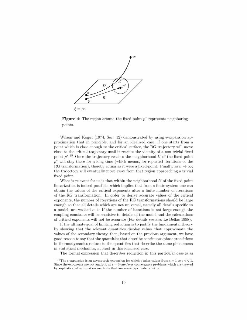
ttpp

ξ =∞

tp∗d′

s

����

�����1&%

'$

R

D

p0t

Figure 4: The region around the fixed point p∗ represents neighboring

points.

Wilson and Kogut (1974, Sec. 12) demonstrated by using ε-expansion ap-proximation that in principle, and for an idealized case, if one starts from apoint which is close enough to the critical surface, the RG trajectory will moveclose to the critical trajectory until it reaches the vicinity of a non-trivial fixedpoint p∗.15 Once the trajectory reaches the neighborhood U of the fixed pointp∗ will stay there for a long time (which means, for repeated iterations of theRG transformation), thereby acting as it were a fixed-point. Finally, as n→∞,the trajectory will eventually move away from that region approaching a trivialfixed point.

What is relevant for us is that within the neighborhood U of the fixed pointlinearization is indeed possible, which implies that from a finite system one canobtain the values of the critical exponents after a finite number of iterationsof the RG transformation. In order to derive accurate values of the criticalexponents, the number of iterations of the RG transformations should be largeenough so that all details which are not universal, namely all details specific toa model, are washed out. If the number of iterations is not large enough thecoupling constants will be sensitive to details of the model and the calculationsof critical exponents will not be accurate (For details see also Le Bellac 1998).

If the ultimate goal of limiting reduction is to justify the fundamental theoryby showing that the relevant quantities display values that approximate thevalues of the secondary theory, then, based on the previous argument, we havegood reason to say that the quantities that describe continuous phase transitionsin thermodynamics reduce to the quantities that describe the same phenomenain statistical mechanics, at least in this idealized case.

The formal expression that describes reduction in this particular case is as

15The ε-expansion is an asymptotic expansion for which ε takes values from ε = 1 to ε << 1.Since the exponents are not analytic at ε = 0 one faces convergence problems which are treatedby sophisticated summation methods that are nowadays under control.

19

follows:

LR5: A physical quantity QSM in statistical mechanics reducesasymptotically to the analogous quantity QTD in thermodynamics,if for N sufficiently large:

∃n0 such that QSMN,n0≈ QTD,

where n0 corresponds to a finite range of iterations of the RG transformation. Itshould be noticed that the values ofQSMN,n0

also approximate limn→∞ limN→∞QSM ,which represent the values of the given quantity after taking both the thermo-dynamic limit and the infinite iteration limit.

One might object that the results obtained in this section rely too muchon an idealized case and that in actual practice things are more complicated.Although it is true that in practice things are less straightforward, numeri-cal simulation gives an important support for what has been said here. Since1976 there have been attempts to use the numerical Monte Carlo simulation inthe framework of renormalization group methods for the study of critical ex-ponents. The first contribution in this direction was made by Ma (1976), whosuggested an application of real space RG methods that required the calculationof the renormalized Hamiltonians. However, since calculating the renormalizedcouplings accurately enough proved to be too difficult, this approach did notsucceed in determining the fixed point Hamiltonian with significant precision.Pawley, Swendsen, and Wilson (1984) made further progress in this direction bysuggesting an approach based on expectation values of the correlation functionsthat did not rely on the calculation of renormalized Hamiltonians. Using thisapproach, they showed that for an Ising square lattice with 64 number sites, thesystem approaches the behavior of an infinite system after two iterations of aRG transformation. After more iterations, however, the system was shown todepart from the expected results flowing towards a trivial fixed point. A plausi-ble explanation for this cross-over was that after more iterations the correlationlength became comparable to the size of the system and finitary effects becamerelevant.16

One should bear in mind, however, that for some models the convergence isnot as rapid as for the 2D-Ising lattice. Therefore, in order to avoid finite sizeeffects in the renormalized systems, one should use large lattices. In the pastyears there has been significant improvement in this direction. See, for example,Hsiao and Monceau (2002) and Itakura (2003).

6 Concluding Remarks

The arguments presented in this paper give us good reason to think that the ap-peal to the infinite limits in the theory of phase transitions does not represent achallenge for reduction, at least not for limiting reduction. In fact, contra what

16This is also pointed out by Butterfield (Butterfield, 2011, p. 69).

20

has been argued by Batterman (2001, 2009) and Morrison (2012), these argu-ments suggest that the infinities and divergences characteristic of the physics ofphase transitions are not essential for giving an account of the phenomena sincefrom finite statistical mechanics one can recover the thermodynamic behaviorof phase transitions even in the case of continuous phase transitions, as it wasshown in section 5.

Nevertheless, this does not mean that phase transitions are not inconsistentwith other notions of reduction that have also been discussed in the philosoph-ical literature. Norton (2013), for instance, correctly points out that the caseof continuous phase transitions does not satisfy what he calls “few-many reduc-tion”, according to which there will be a reduction if the behavior of a systemwith a few components can be used to explain the behavior of a system witha large number of them. The reason for this is that continuous phase tran-sitions are intrinsically fluctuation phenomena that can only arise when N issufficiently large.

Likewise, continuous phase transitions also seem to be at odds with the kindof reductive explanation that requires the explanans to give us accurate and de-tailed information about the microscopic causal mechanisms that produce thephenomenon (e.g. Kaplan (2011)). As it has been pointed out by Batterman(2002), Batterman and Rice (2014) and Morrison (2012), the impossibility ofgiving such an account is related with the robustness of the fixed point solutionsunder different choices of the initial conditions. This implies that the criticalbehavior is largely independent of specific microscopic details characterizing thedifferent models and that the statistical mechanical account of phase transitionsdoes not give us complete information about the microscopic mechanisms un-derlying the transitions. However, as it was shown in the paper, these senses inwhich reduction ”fails” do not threat the project of inter-theory reductionismin any relevant sense.

References

Bangu, S. (2009). Understanding thermodynamic singularities: Phase transi-tions, data, and phenomena. Philosophy of Science.

Bangu, S. (2011). On the role of bridge laws in intertheoretic relations. Philos-ophy of Science, 78(5), 1108-1119.

Batterman, R. W. (2001). The devil in the details: Asymptotic reasoning inexplanation, reduction, and emergence. Oxford University Press.

Batterman, R. W. (2005). Critical phenomena and breaking drops: Infiniteidealizations in physics. Studies in History and Philosophy of SciencePart B: Studies in History and Modern Physics, 36(2), 225-244.

Batterman, R. W. (2011). Emergence, singularities and symmetry breaking.Foundations of Physics, 41(6), 1031-1050.

Batterman, R. W. (2016). Intertheory relations in physics. The Stanford ency-clopedia of philosophy (2016 Edition).

21

Batterman, R. W., & Rice, C. (2014). Minimal model explanations. Philosophyof Science.

Butterfield, J. (2011). Less is different: emergence and reduction reconciled.Foundations of Physics, 41(6)(1065-1135).

Butterfield, J., & Buoatta, N. (2011). Emergence and reduction combined inphase transitions. Frontiers of Fundamental Physics, FFP11 .

Callender, C. (2001). Taking thermodynamics too serously. Studies in Historyand Philosophy of Science Part B: Studies in History and Philosophy ofModern Physics, 32(4), 539-553.

Domb, C. (2000). Phase transitions and critical phenomena (Vol. Vol. 19).Academic Press.

Fisher, M. E. (1998). Renormalization group theory: its basis and formulationin statistical physics. Reviews of Modern Physics, 70(2), 653.

Fletcher, S. C. (2015). Similarity, topology and physical significance in relativitytheory. The British Journal for the Philosophy of Science.

Franklin, A. (2017). On the renormalisation group explanation of universalityon the renormalisation group explanation of universality on the renormal-ization group explanation of universality. Philosophy of Science.

Goldenfeld, N. (1992). Lectures on phase transitions and the renormalizationgroup. Westview Press.

Hsiao, P., & Monceau, P. (2002). Critical behavior of the three-state pottsmodel on the sierpinski carpet. Physical Review B , 65(18)(184427).

Huttermann, A., & Love, A. (2016). Reduction. In P. e. Humphried (Ed.), Theoxford handbook of philosophy of science. new york. Oxford UniversotyPress.

Itakura, M. (2003). Monte carlo renormalization group study of the heisenbergand the xy antiferromagnet on the stacked triangular lattice and the chiralφ 4 model. Journal of the Physical Society of Japan.

Kadanoff, L. P. (2009). More is the same: Phase transitions and mean fieldtheories. Journal of Statistical Physics, 137(5-6).

Kaplan, D. (2011). Explanation and description in computational neuroscience.Synthese.

Landsman, N. P. (2013). Spontaneous symmetry breaking in quantum systems:Emergence or reduction? Studies in History and Philosophy of SciencePart B: Studies in History and Modern Physics, 44(4)(379-394).

Le Bellac, M., Mortessagne, F., & Batrouni, G. (2006). Equilibrium and non-equilibrium statistical thermodynamics. Cambridge University Press.

Ma, S.-K. (1976). Renormalization group by monte carlo methods. PhysicalReview Letters, 37(8)(461).

Menon, T., & Callender, C. (2013). Ch-ch-changes philosophical questions raisedby phase transitions. The Oxford handbook of philosophy of physics.

Morrison, M. (2012). Emergent physics and micro-ontology. Philosophy ofScience.

Nickles, T. (1973). Two concepts of intertheoretic reduction. The Journal ofPhilosophy , 70(7)(181-201).

Norton, J. D. (2012). Approximation and idealizations: Why the difference

22

matters. Philosophy of Science, 79(2), 207-232.Norton, J. D. (2013). Confusions over reduction and emergence

in the physics of phase transitions’. available on Norton’s web-site at: http://www.pitt.edu/jdnorton/Goodies/reduction emergence/redem.html .

Pawley, G., Swendsen, D., R.H. Wallace, & Wilson, K. G. (1984). Monte carlorenormalization-group calculations of critical behavior in the simple-cubicising model. Physical Review , 29 (4030).

Rohrlich, F. (1988). Pluralistic ontology and theory reduction in the physicalsciences. The British Journal for the Philosophy of Science, 39.3 , 295-312.

Rueger, A. (2000). Physical emergence, diacronic and synchronic. Synthese,124 , 297-322.

Scheibe, E. (1998). Die reduktion physikalische theorien: Ein beitrag zur einheitder physik. Springer-Verlag Berlin Heidelberg.

Sornette, D. (2000). Critical phenomena in natural sciences. Springer-Verlag.Wilson, K., & Kogut, J. (1974). The renormalization group and the e expansion.

Physics Reports, 12(2), 75-199.

23