Phase Plane Methods - Home - Mathgustafso/s2017/2280/dynamicalSystems.pdf · Planar Almost Linear...
58
Chapter 10 Phase Plane Methods Contents 10.1 Planar Autonomous Systems ......... 680 10.2 Planar Constant Linear Systems ....... 694 10.3 Planar Almost Linear Systems ........ 705 10.4 Biological Models ................ 715 10.5 Mechanical Models ............... 730 Studied here are planar autonomous systems of differential equations. The topics: Planar Autonomous Systems: Phase Portraits, Stability. Planar Constant Linear Systems: Classification of isolated equilib- ria, Phase portraits. Planar Almost Linear Systems: Phase portraits, Nonlinear classi- fications of equilibria. Biological Models: Predator-prey models, Competition models, Survival of one species, Co-existence, Alligators, doomsday and extinction. Mechanical Models: Nonlinear spring-mass system, Soft and hard springs, Energy conservation, Phase plane and scenes.
Transcript of Phase Plane Methods - Home - Mathgustafso/s2017/2280/dynamicalSystems.pdf · Planar Almost Linear...
Chapter 10
Phase Plane Methods
Contents
10.1 Planar Autonomous Systems . . . . . . . . . 680
10.2 Planar Constant Linear Systems . . . . . . . 694
10.3 Planar Almost Linear Systems . . . . . . . . 705
10.4 Biological Models . . . . . . . . . . . . . . . . 715
10.5 Mechanical Models . . . . . . . . . . . . . . . 730
Studied here are planar autonomous systems of differential equations.The topics:
Planar Autonomous Systems: Phase Portraits, Stability.
Planar Constant Linear Systems: Classification of isolated equilib-ria, Phase portraits.
Planar Almost Linear Systems: Phase portraits, Nonlinear classi-fications of equilibria.
Biological Models: Predator-prey models, Competition models,Survival of one species, Co-existence, Alligators, doomsday andextinction.
Mechanical Models: Nonlinear spring-mass system, Soft and hardsprings, Energy conservation, Phase plane and scenes.
680 Phase Plane Methods
10.1 Planar Autonomous Systems
A set of two scalar differential equations of the form
x′(t) = f(x(t), y(t)),y′(t) = g(x(t), y(t)).
(1)
is called a planar autonomous system. The term autonomousmeans self-governing, justified by the absence of the time variable tin the functions f(x, y), g(x, y).
To obtain the vector form, let ~u(t) =
(x(t)y(t)
), ~F (x, y) =
(f(x, y)g(x, y)
)and write (1) as the first order vector-matrix system
d
dt~u(t) = ~F (~u(t)).(2)
It is assumed that f , g are continuously differentiable in some region Din the xy-plane. This assumption makes ~F continuously differentiable inD and guarantees that Picard’s existence-uniqueness theorem for initialvalue problems applies to the initial value problem d
dt~u(t) = ~F (~u(t)),~u(0) = ~u0. Accordingly, to each ~u0 = (x0, y0) in D there corresponds aunique solution ~u(t) = (x(t), y(t)), represented as a planar curve in thexy-plane, which passes through ~u0 at t = 0.
Such a planar curve is called a trajectory or orbit of the system andits parameter interval is some maximal interval of existence T1 < t < T2,where T1 and T2 might be infinite. A graphic of trajectories drawn asparametric curves in the xy-plane is called a phase portrait and thexy-plane in which it is drawn is called the phase plane.
Trajectories Don’t Cross
Autonomy of the planar system plus uniqueness of initial value problemsimplies that trajectories (x1(t), y1(t)) and (x2(t), y2(t)) cannot touch orcross. Hand-drawn phase portraits are accordingly limited: you cannotdraw a solution trajectory that touches another solution curve!
Theorem 1 (Identical Trajectories)Assume that Picard’s existence-uniqueness theorem applies to initial valueproblems in D for the planar system
d
dt~u(t) = ~F (~u(t)), ~u(t) =
(x(t)y(t)
).
Let (x1(t), y1(t)) and (x2(t), y2(t)) be two trajectories of the system. Iftimes t1, t2 exist such that
x1(t1) = x2(t2), y1(t1) = y2(t2),(3)
10.1 Planar Autonomous Systems 681
then for the value c = t1−t2 the equations x1(t+c) = x2(t) and y1(t+c) =y2(t) are valid for all allowed values of t. This means that the two trajectoriesare on one and the same planar curve, or in the contrapositive, two differenttrajectories cannot touch or cross in the phase plane.
Proof: Define x(t) = x1(t+ c), y(t) = y1(t+ c). By the chain rule, (x(t), y(t))is a solution of the planar system, because x′(t) = x′1(t+c) = f(x1(t+c), y1(t+c)) = f(x(t), y(t)), and similarly for the second differential equation. Further,(3) implies x(t2) = x2(t2) and y(t2) = y2(t2), therefore Picard’s uniquenesstheorem implies that x(t) = x2(t) and y(t) = y2(t) for all allowed values of t.The proof is complete.
Equilibria
A trajectory that reduces to a point, or a constant solution x(t) = x0,y(t) = y0, is called an equilibrium solution. The equilibrium solutionsor equilibria are found by solving the nonlinear equations
f(x0, y0) = 0, g(x0, y0) = 0.
Each such (x0, y0) in D is a trajectory whose graphic in the phase planeis a single point, called an equilibrium point. In applied literature,it may be called a critical point, stationary point or rest point.Theorem 1 has the following geometrical interpretation.
Assuming uniqueness, no other trajectory (x(t), y(t)) in thephase plane can touch an equilibrium point (x0, y0).
Equilibria (x0, y0) are often found from linear equations
ax0 + by0 = e, cx0 + dy0 = f,
which are solved by linear algebra methods. They constitute an impor-tant subclass of algebraic equations which can be solved symbolically. Inthis special case, symbolic solutions exist for the equilibria.
It is interesting to report that in a practical sense the equilibria may bereported incorrectly, due to the limitations of computer software, evenin the case when exact symbolic solutions are available. An example isx′ = x+ y, y′ = εy− ε for small ε > 0. The root of the problem is trans-lation of ε to a machine constant, which is zero for small enough ε. Theresult is that computer software detects infinitely many equilibria whenin fact there is exactly one equilibrium point. This example suggeststhat symbolic computation be used by default.
682 Phase Plane Methods
Practical Methods for Computing Equilibria
There exists no supporting theory to find equilibria for all choices ofF and G. However, there is a rich library of special methods for solv-ing nonlinear algebraic equations, including numerical methods basedon celebrated univariate methods, such as Newton’s method and thebisection method.
Computer algebra systems like maple, maxima and mathematica offerconvenient codes to solve the equations, when possible, including sym-bolic solutions. Applied mathematics depends on the dynamically ex-panding library of special methods, which grows due to new mathemat-ical discoveries. See the exercises for examples.
Population Biology
Planar autonomous systems have been applied to two-species popula-tions like two species of trout, who compete for food from the samesupply, and foxes and rabbits, who compete in a predator-prey situa-tion.
Certain equilibria are significant, because they represent the populationsizes for cohabitation. A point in the phase space that is not an equi-librium point corresponds to population sizes that cannot coexist, theymust change with time. Some equilibria are consequently observableor average population sizes while non-equilibria correspond to snapshotpopulation sizes that are subject to flux. Biologists expect populationsizes of such two-species competition models to undergo change untilthey reach approximately the observable values, on the average.
Rabbit-Fox System
This example is a predator-prey system, in which the expected observ-able population sizes are averages, about which the actual populationssize oscillate about, periodically over time. Certain equilibria for thesesystems represent ideal cohabitation. Biological experiments suggestthat initial population sizes close to the equilibrium values cause popula-tions to stay near the initial sizes, even though the populations oscillateperiodically. Observations by field biologists of large population vari-ations seem to verify that individual populations oscillate periodicallyaround the ideal cohabitation sizes.
A typical planar system for predator-prey dynamics of x(t) rabbits and
10.1 Planar Autonomous Systems 683
y(t) foxes is the system
dx
dt=
1
200x(40− y),
dy
dt=
1
100y(x− 50).
Time variable t is in months. The equilibria are (0, 0), (50, 40). Withinitial populations x(0) = 60 rabbits and y(0) = 30 foxes, both x′ and y′
are positive near t = 0, which implies the populations initially increasein size.
After time, the signs of x′ and y′ are alternately positive and negative,which reflects the oscillating behavior of the populations about the idealequilibrium values x = 50, y = 40. The period of oscillation is about20 months. This predator-prey model predicts coexistence with averagepopulations of 50 rabbits and 40 foxes.
Trout System
Consider a population of two species of trout who compete for the samefood supply. A typical autonomous planar system for the species x andy is
dx
dt= x(−2x− y + 180),
dy
dt= y(−x− 2y + 120).
Equilibria. The equilibrium solutions for the trout system are
(0, 0), (90, 0), (0, 60), (80, 20).
Only nonnegative population sizes are physically significant. Units forthe population sizes might be in hundreds or thousands of fish. The equi-librium (0, 0) corresponds to extinction of both species, while (0, 60)and (90, 0) correspond to the unusual situation of extinction for onespecies. The last equilibrium (80, 20) corresponds to co-existence ofthe two trout species with observable population sizes of 80 and 20.
Phase Portraits
A graphic which contains some equilibria and typical trajectories of aplanar autonomous system (1) is called a phase portrait.
While graphing equilibria is not a challenge, graphing typical trajecto-ries, also called orbits, seems to imply that we are going to solve thedifferential system. This is not the case. Approximations will be usedthat do not require solution of the differential system.
684 Phase Plane Methods
Equilibria Plot in the xy-plane all equilibria of (1). See Figure 3.
Window Select an x-range and a y-range for the graph windowwhich includes all significant equilibria (Figure 3).
Grid Plot a uniform grid of N grid points (N ≈ 50 for handwork) within the graph window, to populate the graph-ical white space (Figure 4). The isocline method mightalso be used to select grid points.
Field Draw at each grid point a short tangent vector, a re-placement curve for a solution curve through a gridpoint on a small time interval (Figure 5).
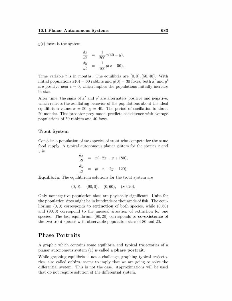
Orbits Draw additional threaded trajectories on long time inter-vals into the remaining white space of the graphic (Figure6). This is guesswork, based upon tangents to threadedtrajectories matching nearby field tangents drawn in theprevious step. See Figures 1 and 2 for details.
C
y
xb
aFigure 1. Badly threaded orbit.
Threaded solution curve C correctly matches itstangent to the tangent at nearby grid point a,but it fails to match at grid point b.
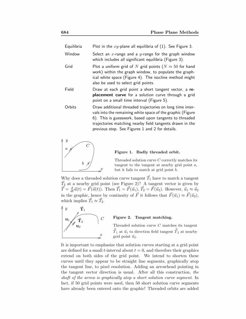
Why does a threaded solution curve tangent ~T1 have to match a tangent~T2 at a nearby grid point (see Figure 2)? A tangent vector is given by~T = d
dt~u(t) = ~F (~u(t)). Then ~T1 = ~F (~u1), ~T2 = ~F (~u2). However, ~u1 ≈ ~u2in the graphic, hence by continuity of ~F it follows that ~F (~u1) ≈ ~F (~u2),which implies ~T1 ≈ ~T2.
u2
C
x
y ~T1
~T2u1
Figure 2. Tangent matching.
Threaded solution curve C matches its tangent~~T 1 at ~u1 to direction field tangent
~~T 2 at nearbygrid point ~u2.
It is important to emphasize that solution curves starting at a grid pointare defined for a small t-interval about t = 0, and therefore their graphicsextend on both sides of the grid point. We intend to shorten thesecurves until they appear to be straight line segments, graphically atopthe tangent line, to pixel resolution. Adding an arrowhead pointing inthe tangent vector direction is usual. After all this construction, theshaft of the arrow is graphically atop a short solution curve segment. Infact, if 50 grid points were used, then 50 short solution curve segmentshave already been entered onto the graphic! Threaded orbits are added
10.1 Planar Autonomous Systems 685
to show what happens to solutions that are plotted on longer and longert-intervals.
Phase Portrait Illustration
The method outlined above will be applied to the illustration
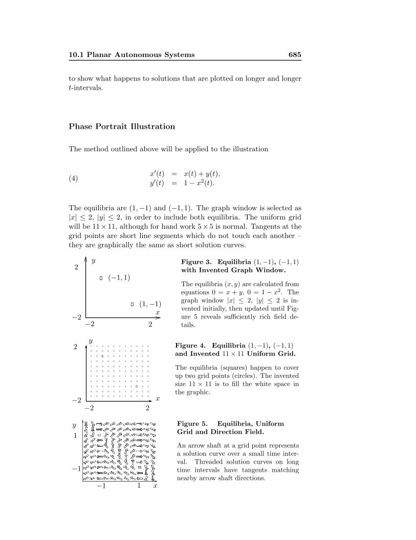
x′(t) = x(t) + y(t),y′(t) = 1− x2(t).(4)
The equilibria are (1,−1) and (−1, 1). The graph window is selected as|x| ≤ 2, |y| ≤ 2, in order to include both equilibria. The uniform gridwill be 11× 11, although for hand work 5× 5 is normal. Tangents at thegrid points are short line segments which do not touch each another –they are graphically the same as short solution curves.
−2−2
2y
2
(1,−1)x
(−1, 1)
Figure 3. Equilibria (1,−1), (−1, 1)with Invented Graph Window.
The equilibria (x, y) are calculated fromequations 0 = x + y, 0 = 1 − x2. Thegraph window |x| ≤ 2, |y| ≤ 2 is in-vented initially, then updated until Fig-ure 5 reveals sufficiently rich field de-tails.
−2 2
x−2
2y
Figure 4. Equilibria (1,−1), (−1, 1)and Invented 11× 11 Uniform Grid.
The equilibria (squares) happen to coverup two grid points (circles). The inventedsize 11 × 11 is to fill the white space inthe graphic.
−1
y
−1 1 x
1
Figure 5. Equilibria, UniformGrid and Direction Field.
An arrow shaft at a grid point representsa solution curve over a small time inter-val. Threaded solution curves on longtime intervals have tangents matchingnearby arrow shaft directions.
686 Phase Plane Methods
y
1
−1
−1 1 x
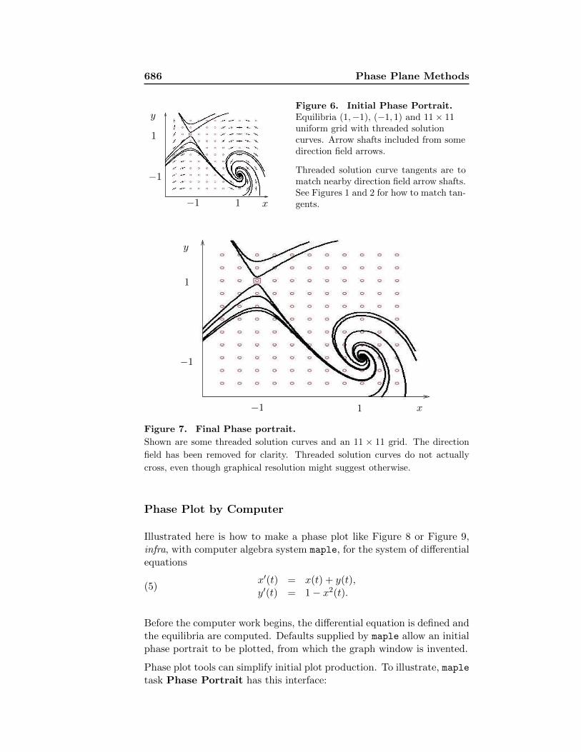
Figure 6. Initial Phase Portrait.Equilibria (1,−1), (−1, 1) and 11× 11uniform grid with threaded solutioncurves. Arrow shafts included from somedirection field arrows.
Threaded solution curve tangents are tomatch nearby direction field arrow shafts.See Figures 1 and 2 for how to match tan-gents.
1
−1 1 x
−1
y
Figure 7. Final Phase portrait.
Shown are some threaded solution curves and an 11 × 11 grid. The direction
field has been removed for clarity. Threaded solution curves do not actually
cross, even though graphical resolution might suggest otherwise.
Phase Plot by Computer
Illustrated here is how to make a phase plot like Figure 8 or Figure 9,infra, with computer algebra system maple, for the system of differentialequations
x′(t) = x(t) + y(t),y′(t) = 1− x2(t).(5)
Before the computer work begins, the differential equation is defined andthe equilibria are computed. Defaults supplied by maple allow an initialphase portrait to be plotted, from which the graph window is invented.
Phase plot tools can simplify initial plot production. To illustrate, mapletask Phase Portrait has this interface:
10.1 Planar Autonomous Systems 687
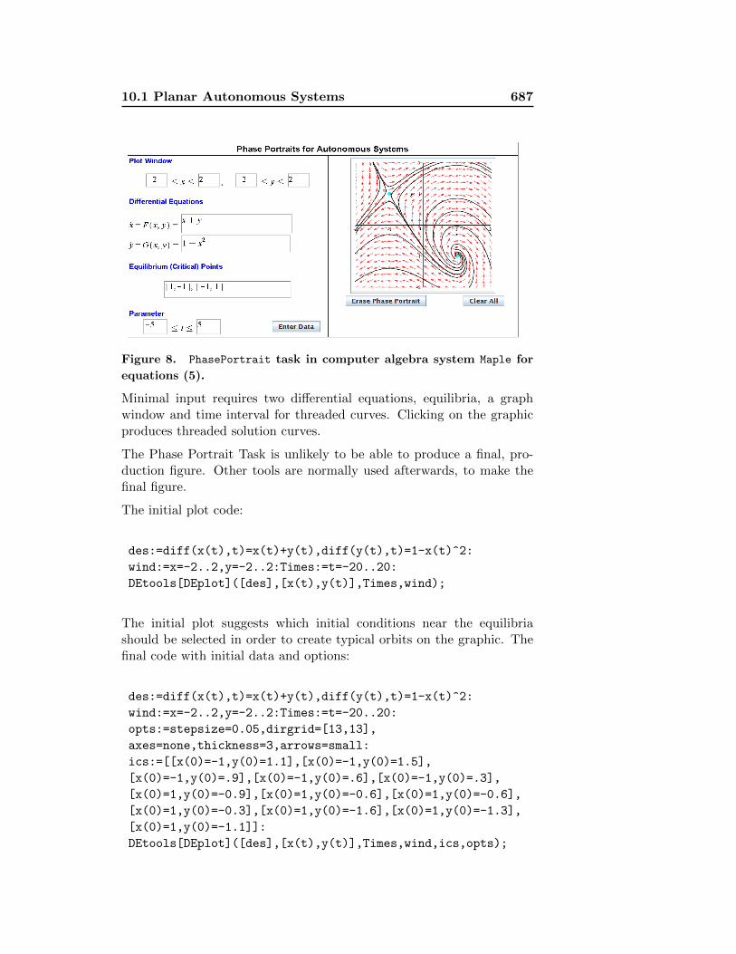
Figure 8. PhasePortrait task in computer algebra system Maple for
equations (5).
Minimal input requires two differential equations, equilibria, a graphwindow and time interval for threaded curves. Clicking on the graphicproduces threaded solution curves.
The Phase Portrait Task is unlikely to be able to produce a final, pro-duction figure. Other tools are normally used afterwards, to make thefinal figure.
The initial plot code:
des:=diff(x(t),t)=x(t)+y(t),diff(y(t),t)=1-x(t)^2:
wind:=x=-2..2,y=-2..2:Times:=t=-20..20:
DEtools[DEplot]([des],[x(t),y(t)],Times,wind);
The initial plot suggests which initial conditions near the equilibriashould be selected in order to create typical orbits on the graphic. Thefinal code with initial data and options:
des:=diff(x(t),t)=x(t)+y(t),diff(y(t),t)=1-x(t)^2:
wind:=x=-2..2,y=-2..2:Times:=t=-20..20:
opts:=stepsize=0.05,dirgrid=[13,13],
axes=none,thickness=3,arrows=small:
ics:=[[x(0)=-1,y(0)=1.1],[x(0)=-1,y(0)=1.5],
[x(0)=-1,y(0)=.9],[x(0)=-1,y(0)=.6],[x(0)=-1,y(0)=.3],
[x(0)=1,y(0)=-0.9],[x(0)=1,y(0)=-0.6],[x(0)=1,y(0)=-0.6],
[x(0)=1,y(0)=-0.3],[x(0)=1,y(0)=-1.6],[x(0)=1,y(0)=-1.3],
[x(0)=1,y(0)=-1.1]]:
DEtools[DEplot]([des],[x(t),y(t)],Times,wind,ics,opts);
688 Phase Plane Methods
1−1
1
−1
y
x
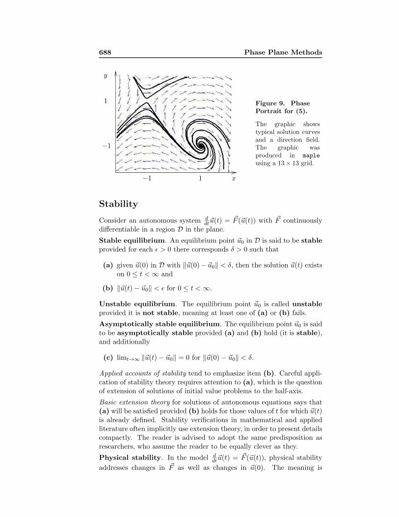
Figure 9. PhasePortrait for (5).
The graphic showstypical solution curvesand a direction field.The graphic wasproduced in maple
using a 13× 13 grid.
Stability
Consider an autonomous system ddt~u(t) = ~F (~u(t)) with ~F continuously
differentiable in a region D in the plane.
Stable equilibrium. An equilibrium point ~u0 in D is said to be stableprovided for each ε > 0 there corresponds δ > 0 such that
(a) given ~u(0) in D with ‖~u(0)− ~u0‖ < δ, then the solution ~u(t) existson 0 ≤ t <∞ and
(b) ‖~u(t)− ~u0‖ < ε for 0 ≤ t <∞.
Unstable equilibrium. The equilibrium point ~u0 is called unstableprovided it is not stable, meaning at least one of (a) or (b) fails.
Asymptotically stable equilibrium. The equilibrium point ~u0 is saidto be asymptotically stable provided (a) and (b) hold (it is stable),and additionally
(c) limt→∞ ‖~u(t)− ~u0‖ = 0 for ‖~u(0)− ~u0‖ < δ.
Applied accounts of stability tend to emphasize item (b). Careful appli-cation of stability theory requires attention to (a), which is the questionof extension of solutions of initial value problems to the half-axis.
Basic extension theory for solutions of autonomous equations says that(a) will be satisfied provided (b) holds for those values of t for which ~u(t)is already defined. Stability verifications in mathematical and appliedliterature often implicitly use extension theory, in order to present detailscompactly. The reader is advised to adopt the same predisposition asresearchers, who assume the reader to be equally clever as they.
Physical stability. In the model ddt~u(t) = ~F (~u(t)), physical stability
addresses changes in ~F as well as changes in ~u(0). The meaning is
10.1 Planar Autonomous Systems 689
this: physical parameters of the model, e.g., the mass m > 0, dampingconstant c > 0 and Hooke’s constant k > 0 in a damped spring-masssystem
x′ = y,
y′ = − c
my − k
mx,
may undergo small changes without significantly affecting the solution.
In physical stability, stable equilibria correspond to physically ob-served data whereas other solutions correspond to transient obser-vations that disappear over time.
A typical instance is the trout system
x′(t) = x(−2x− y + 180),y′(t) = y(−x− 2y + 120).
(6)
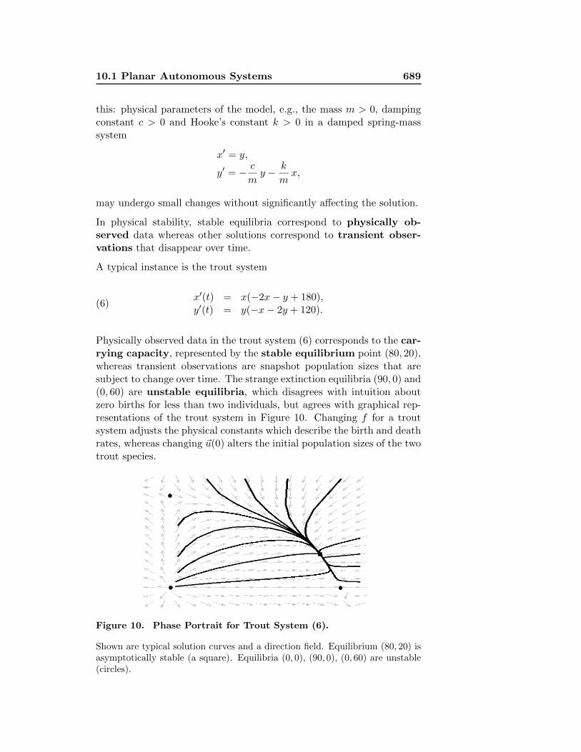
Physically observed data in the trout system (6) corresponds to the car-rying capacity, represented by the stable equilibrium point (80, 20),whereas transient observations are snapshot population sizes that aresubject to change over time. The strange extinction equilibria (90, 0) and(0, 60) are unstable equilibria, which disagrees with intuition aboutzero births for less than two individuals, but agrees with graphical rep-resentations of the trout system in Figure 10. Changing f for a troutsystem adjusts the physical constants which describe the birth and deathrates, whereas changing ~u(0) alters the initial population sizes of the twotrout species.
Figure 10. Phase Portrait for Trout System (6).
Shown are typical solution curves and a direction field. Equilibrium (80, 20) isasymptotically stable (a square). Equilibria (0, 0), (90, 0), (0, 60) are unstable(circles).
690 Phase Plane Methods
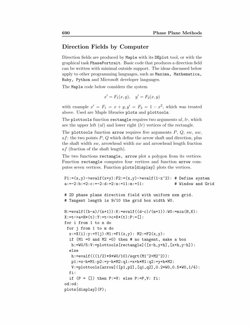
Direction Fields by Computer
Direction fields are produced by Maple with its DEplot tool, or with thegraphical task PhasePortrait. Basic code that produces a direction fieldcan be written with minimal outside support. The ideas discussed belowapply to other programming languages, such as Maxima, Mathematica,
Ruby, Python and Microsoft developer languages.
The Maple code below considers the system
x′ = F1(x, y), y′ = F2(x, y)
with example x′ = F1 = x + y, y′ = F2 = 1 − x2, which was treatedabove. Used are Maple libraries plots and plottools.
The plottools function rectangle requires two arguments ul, lr, whichare the upper left (ul) and lower right (lr) vertices of the rectangle.
The plottools function arrow requires five arguments P , Q, sw, aw,af : the two points P , Q which define the arrow shaft and direction, plusthe shaft width sw, arrowhead width aw and arrowhead length fractionaf (fraction of the shaft length).
The two functions rectangle, arrow plot a polygon from its vertices.Function rectangle computes four vertices and function arrow com-putes seven vertices. Function plots[display] plots the vertices.
F1:=(x,y)->evalf(x+y):F2:=(x,y)->evalf(1-x^2): # Define system
a:=-2:b:=2:c:=-2:d:=2:n:=11:m:=11: # Window and Grid
# 2D phase plane direction field with uniform nxm grid.
# Tangent length is 9/10 the grid box width W0.
H:=evalf((b-a)/(n+1)):K:=evalf((d-c)/(m+1)):W0:=min(H,K):
X:=t->a+H*(t):Y:=t->c+K*(t):P:=[]:
for i from 1 to n do
for j from 1 to m do
x:=X(i):y:=Y(j):M1:=F1(x,y): M2:=F2(x,y):
if (M1 =0 and M2 =0) then # no tangent, make a box
h:=W0/5:V:=plottools[rectangle]([x-h,y+h],[x+h,y-h]):
else
h:=evalf(((1/2)*9*W0/10)/sqrt(M1^2+M2^2)):
p1:=x-h*M1:p2:=y-h*M2:q1:=x+h*M1:q2:=y+h*M2:
V:=plottools[arrow]([p1,p2],[q1,q2],0.2*W0,0.5*W0,1/4):
fi:
if (P = []) then P:=V: else P:=P,V: fi:
od:od:
plots[display](P);
10.1 Planar Autonomous Systems 691
Exercises 10.1
Autonomous Planar Systems.
Consider
x′(t) = x(t) + y(t),y′(t) = 1− x2(t).
(7)
1. (Vector-Matrix Form) System (7)can be written in vector-matrixform
d
dt~u = ~F (~u(t)).
Display formulas for ~u and ~F .
2. (Picard’s Theorem) Picard’s vec-tor existence-uniqueness theoremapplies to system (7) with initialdata x(0) = x0, y(0) = y0. Showthe details.
Trajectories Don’t Cross.
3. (Theorem 1 Details) Computedydt = g(x1(t + c), y1(t + c)), thenshow that y′(t) = g(x(t), y(t)) inthe proof of Theorem 1.
4. (Orbits Can Cross) The example
dx
dt= 1,
dy
dt= 3y2/3
has infinitely many orbits crossingat x = y = 0. Exhibit two distinctorbits which cross at x = y = 0.Does this example contradict The-orem 1?
Equilibria. A point (x0, y0) is calledan equilibrium provided x(t) = x0,y(t) = y0 is a solution of the dynami-cal system.
5. Justify that (1,−1), (−1, 1) are theonly equilibria for the system x′ =x+ y, y′ = 1− x2.
6. Display the details which justifythat (0, 0), (90, 0), (0, 60), (80, 20)are all equilibria for the sys-tem x′(t) = x(−2x − y + 180),y′(t) = y(−x− 2y + 120).
Practical Methods for ComputingEquilibria.
7. (Murray System) The biologicalsystem
x′ = x(6−2x−y), y′ = y(4−x−y)
has equilibria (0, 0), (3, 0), (0, 4),(2, 2). Justify the four answers.
8. (Nullclines) Curves along whicheither x′ = 0 or y′ = 0 are callednullclines. The biological system
x′ = x(6−2x−y), y′ = y(4−x−y)
has nullclines x = 0, y = 0, 6−2x−y = 0, 4 − x − y = 0. Justify thefour answers.
9. (Nullclines by Computer) Pro-duce a graphical display of the null-clines of the Murray System above.Maple code to produce a nullclineplot is as follows
eqns:={x*(6-2*x-y),y*(4-x-y)};
wind:=x=0..130,y=0..80;
plots[contourplot](eqns,wind,
contours=[0]);
10. (Isoclines by Computer) Levelcurves f(x, y) = c are called iso-clines.
Maple will plot level curvesf(x, y) = −2, f(x, y) = 0,f(x, y) = 2 using the nullclinecode above, with replacementcontours=[-2,0,2]. Producean isocline plot for the MurraySystem above with these samecontours.
11. (Implicit Plot) Equilibria can befound graphically by an implicitplot. Maple code:
eqns:={x*(6-2*x-y),y*(4-x-y)};
wind:=x=0..130,y=0..80;
plots[implicitplot](eqns,wind);
Produce the implicit plot. Is it thesame as the nullcline plot?
692 Phase Plane Methods
Rabbit-Fox System.
12. (Predator-Prey) Consider a rab-bit and fox system
x′ =1
200x(30− y),
y′ =1
100y(x− 40).
Argue why extinction of the rab-bits (x = 0) implies extinction ofthe foxes (y = 0).
13. (Predator-Prey) The rabbit andfox system
x′ =1
200x(40− y),
y′ =1
100y(x− 40),
has extinction of the foxes (y =0) implying Malthusian popu-lation explosion of the rabbits(limt=∞ x(t) =∞). Explain.
Trout System. Consider
x′(t) = x(−2x− y + 180),y′(t) = y(−x− 2y + 120).
14. (Carrying Capacity) Show de-tails for calculation of the carryingcapacities x = 80, y = 20.
15. (Stability) Equilibrium point x =80, y = 20 is stable. Explainthis statement using geometry fromFigure 10 and the definition of sta-bility.
Phase Portraits. Consider
x′(t) = x(t) + y(t),y′(t) = 1− x2(t).
16. (Equilibria) Solve for x, y in thesystem
0 = x+ y,0 = 1− x2,
for equilibria (1,−1), (−1, 1).
17. (Graph Window) Explain why−2 ≤ x ≤ 2, −2 ≤ y ≤ 2 is asuitable window.
18. (Grid Points) Draw a 5×5 grid onthe graph window |x| ≤ 2, |y| ≤ 2.Label the equilibria.
19. (Direction Field) Draw directionfield arrows on the 5 × 5 grid ofthe previous exercise. They co-incide with the tangent direction~v = x′~ı+ y′~ = (x+ y)~ı+ (1−x2)~,where (x, y) is the grid point. Thearrows may not touch.
20. (Threaded Orbits) On the di-rection field of the previous exer-cise, draw orbits (threaded solutioncurves), using the rules:
1. Orbits don’t cross.
2. Orbits pass direction field ar-rows with nearly matchingtangent.
Phase Plot by Computer. Use acomputer algebra system or a numer-ical workbench to produce phase por-traits for the given dynamical system.A graph window should contain allequilibria.
21. (Rabbit-Fox System I)
x′ =1
200x(30− y),
y′ =1
100y(x− 40).
22. (Rabbit-Fox System II)
x′ =1
100x(50− y),
y′ =1
200y(x− 40).
23. (Trout System I)
x′(t) = x(−2x− y + 180),y′(t) = y(−x− 2y + 120).
24. (Trout System II)
x′(t) = x(−2x− y + 200),y′(t) = y(−x− 2y + 120).
10.1 Planar Autonomous Systems 693
Stability Inequalities. The signs ofx′(t) and/or y′(t) can predict stabil-ity or instability. Consider an equi-librium point (x0, y0) and all solutionsx(t), y(t) satisfying for H small the in-equalities
|x(0)− x0| ≤ H, |y(0)− y0| ≤ H.
25. (Instability: Repeller) Provethat x′(t) > 0 and y′(t) > 0 forall small H > 0 implies instabilityat x0, y0.
26. (Stability: Attractor) Prove thatx′(t) < 0 and y′(t) < 0 for all smallH > 0 implies stability at x0, y0.
27. (Instability in x) Prove thatx′(t) > 0 for all small H > 0 im-plies instability at x0, y0.
28. (Instability in y) Prove thaty′(t) > 0 for all small H > 0 im-plies instability at x0, y0.
Geometric Stability.
29. (Attractor) Imagine a dust parti-cle in a fluid draining down a fun-nel, whose trace is a space curve.Project the space curve onto theplane orthogonal to the centerline
of the funnel. Is this planar orbitstable at centerline position in thesense of the definition?
30. (Repeller) Imagine a paintdroplet from a paint spray can,which traces a space curve. Projectthe space curve onto the planeorthogonal to the spray orificedirection. Is this planar orbitstable at centerline position in thesense of the definition?
Algebraic Stability.
31. (Rabbit–Fox Stability) Providealgebraic details for stability ofequilibrium x = 40, y = 30 for thesystem
x′ =1
200x(30− y),
y′ =1
100y(x− 40).
32. (Rabbit–Fox Instability) Providealgebraic details for instability ofequilibrium x = 0, y = 0 for thesystem
x′ =1
100x(50− y),
y′ =1
200y(x− 40).
694 Phase Plane Methods
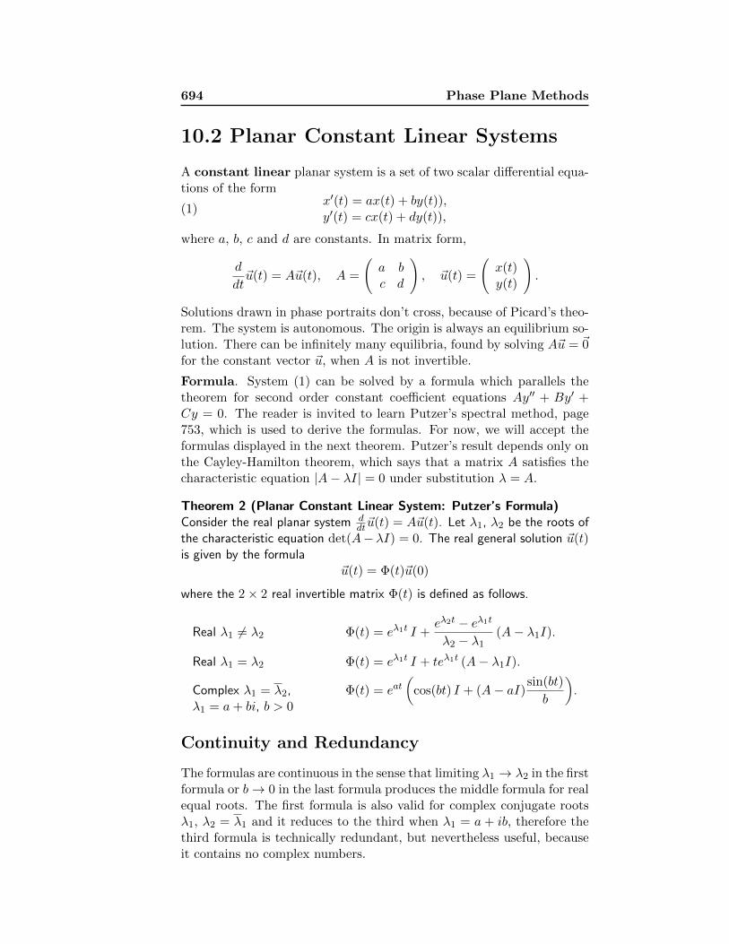
10.2 Planar Constant Linear Systems
A constant linear planar system is a set of two scalar differential equa-tions of the form
x′(t) = ax(t) + by(t)),y′(t) = cx(t) + dy(t)),
(1)
where a, b, c and d are constants. In matrix form,
d
dt~u(t) = A~u(t), A =
(a bc d
), ~u(t) =
(x(t)y(t)
).
Solutions drawn in phase portraits don’t cross, because of Picard’s theo-rem. The system is autonomous. The origin is always an equilibrium so-lution. There can be infinitely many equilibria, found by solving A~u = ~0for the constant vector ~u, when A is not invertible.
Formula. System (1) can be solved by a formula which parallels thetheorem for second order constant coefficient equations Ay′′ + By′ +Cy = 0. The reader is invited to learn Putzer’s spectral method, page753, which is used to derive the formulas. For now, we will accept theformulas displayed in the next theorem. Putzer’s result depends only onthe Cayley-Hamilton theorem, which says that a matrix A satisfies thecharacteristic equation |A− λI| = 0 under substitution λ = A.
Theorem 2 (Planar Constant Linear System: Putzer’s Formula)Consider the real planar system d
dt~u(t) = A~u(t). Let λ1, λ2 be the roots ofthe characteristic equation det(A− λI) = 0. The real general solution ~u(t)is given by the formula
~u(t) = Φ(t)~u(0)
where the 2× 2 real invertible matrix Φ(t) is defined as follows.
Real λ1 6= λ2 Φ(t) = eλ1t I +eλ2t − eλ1t
λ2 − λ1(A− λ1I).
Real λ1 = λ2 Φ(t) = eλ1t I + teλ1t (A− λ1I).
Complex λ1 = λ2,λ1 = a+ bi, b > 0
Φ(t) = eat(
cos(bt) I + (A− aI)sin(bt)
b
).
Continuity and Redundancy
The formulas are continuous in the sense that limiting λ1 → λ2 in the firstformula or b→ 0 in the last formula produces the middle formula for realequal roots. The first formula is also valid for complex conjugate rootsλ1, λ2 = λ1 and it reduces to the third when λ1 = a + ib, therefore thethird formula is technically redundant, but nevertheless useful, becauseit contains no complex numbers.
10.2 Planar Constant Linear Systems 695
Recommended: Memorize the first formula, derive the other two.
About the Newton Quotient. The Newton quotient g(x)−g(x0)x−x0 in
the first formula of the theorem uses g(x) = ext, x = λ2, x0 = λ1,x − x0 = λ2 − λ1. Calculus defines g′(x0) as the Newton quotient limitas x→ x0.
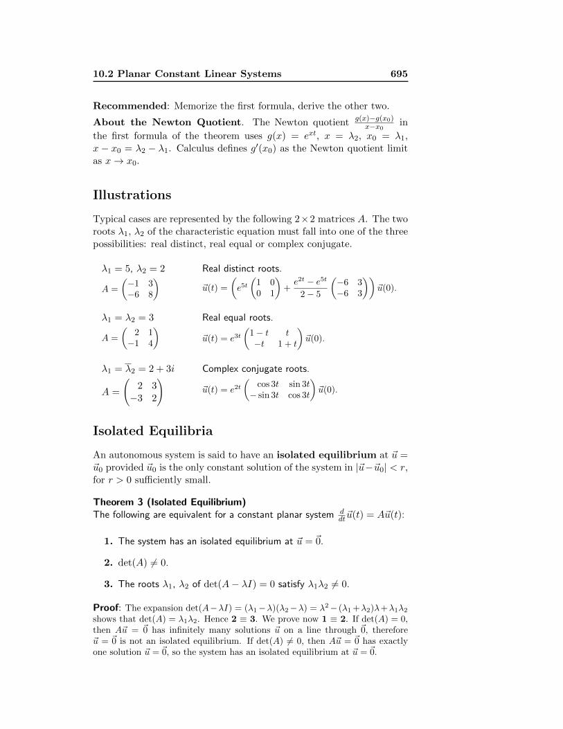
Illustrations
Typical cases are represented by the following 2×2 matrices A. The tworoots λ1, λ2 of the characteristic equation must fall into one of the threepossibilities: real distinct, real equal or complex conjugate.
λ1 = 5, λ2 = 2
A =
(−1 3−6 8
) Real distinct roots.
~u(t) =
(e5t(
1 00 1
)+e2t − e5t
2− 5
(−6 3−6 3
))~u(0).
λ1 = λ2 = 3
A =
(2 1−1 4
) Real equal roots.
~u(t) = e3t(
1− t t−t 1 + t
)~u(0).
λ1 = λ2 = 2 + 3i
A =
(2 3−3 2
) Complex conjugate roots.
~u(t) = e2t(
cos 3t sin 3t− sin 3t cos 3t
)~u(0).
Isolated Equilibria
An autonomous system is said to have an isolated equilibrium at ~u =~u0 provided ~u0 is the only constant solution of the system in |~u−~u0| < r,for r > 0 sufficiently small.
Theorem 3 (Isolated Equilibrium)The following are equivalent for a constant planar system d
dt~u(t) = A~u(t):
1. The system has an isolated equilibrium at ~u = ~0.
2. det(A) 6= 0.
3. The roots λ1, λ2 of det(A− λI) = 0 satisfy λ1λ2 6= 0.
Proof: The expansion det(A−λI) = (λ1−λ)(λ2−λ) = λ2− (λ1 +λ2)λ+λ1λ2shows that det(A) = λ1λ2. Hence 2 ≡ 3. We prove now 1 ≡ 2. If det(A) = 0,then A~u = ~0 has infinitely many solutions ~u on a line through ~0, therefore~u = ~0 is not an isolated equilibrium. If det(A) 6= 0, then A~u = ~0 has exactlyone solution ~u = ~0, so the system has an isolated equilibrium at ~u = ~0.
696 Phase Plane Methods
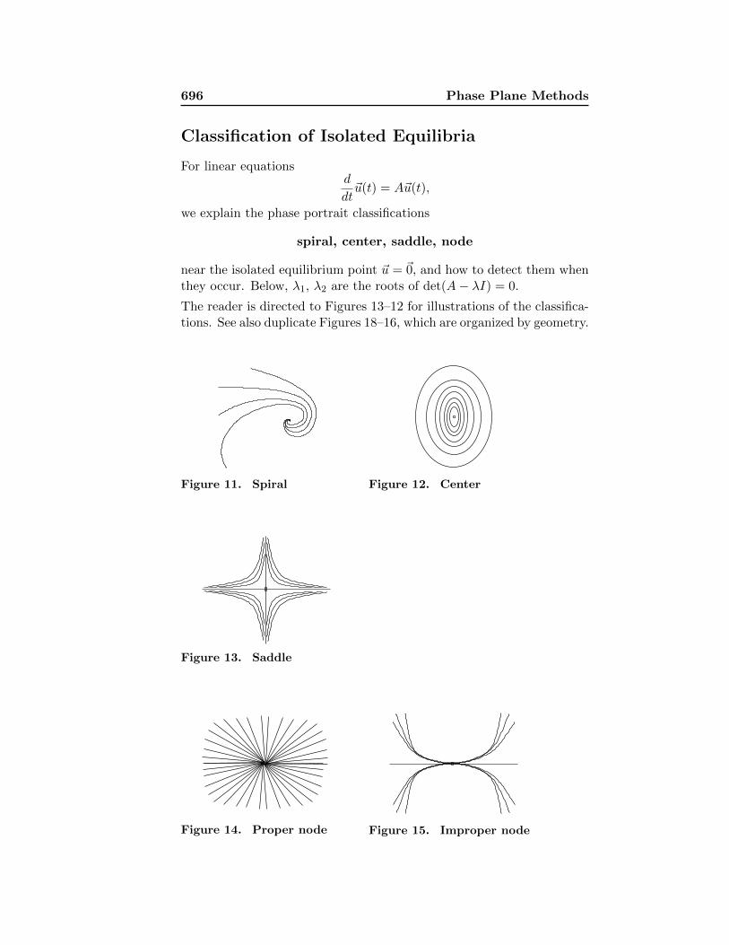
Classification of Isolated Equilibria
For linear equationsd
dt~u(t) = A~u(t),
we explain the phase portrait classifications
spiral, center, saddle, node
near the isolated equilibrium point ~u = ~0, and how to detect them whenthey occur. Below, λ1, λ2 are the roots of det(A− λI) = 0.
The reader is directed to Figures 13–12 for illustrations of the classifica-tions. See also duplicate Figures 18–16, which are organized by geometry.
Figure 11. Spiral Figure 12. Center
Figure 13. Saddle
Figure 14. Proper node Figure 15. Improper node
10.2 Planar Constant Linear Systems 697
Spiral λ1 = λ2 = a+ ib complex, a 6= 0, b > 0.
A spiral has solution formula
~u(t) = eat cos(bt)~c1 + eat sin(bt)~c2,
~c1 = ~u(0), ~c2 =A− aIb
~u(0).
All solutions are bounded harmonic oscillations of naturalfrequency b times an exponential amplitude which grows ifa > 0 and decays if a < 0. An orbit in the phase planespirals out if a > 0 and spirals in if a < 0.
Center λ1 = λ2 = a+ ib complex, a = 0, b > 0
A center has solution formula
~u(t) = cos(bt)~c1 + sin(bt)~c2,
~c1 = ~u(0), ~c2 =1
bA~u(0).
All solutions are bounded harmonic oscillations of naturalfrequency b. Orbits in the phase plane are periodic closedcurves of period 2π/b which encircle the origin.
Saddle λ1, λ2 real, λ1λ2 < 0
A saddle has solution formula
~u(t) = eλ1t~c1 + eλ2t~c2,
~c1 =A− λ2Iλ1 − λ2
~u(0), ~c2 =A− λ1Iλ2 − λ1
~u(0).
The phase portrait shows two lines through the origin whichare tangents at t = ±∞ for all orbits.The line directions are given by the eigenvectors of matrixA. See Figure 13.
Node λ1, λ2 real, λ1λ2 > 0
The solution formulas are
~u(t) = eλ1t (~a1 + t~a2) , when λ1 = λ2,
~a1 = ~u(0), ~a2 = (A− λ1I)~u(0),
~u(t) = eλ1t~b1 + eλ2t~b2, when λ1 6= λ2,
~b1 =A− λ2Iλ1 − λ2
~u(0), ~b2 =A− λ1Iλ2 − λ1
~u(0).
698 Phase Plane Methods
Proper Node (a.k.a. Star Node). Matrix A is requiredto have two eigenpairs (λ1, ~v1), (λ2, ~v2) with λ1 = λ2.Then ~u(0) in span(~v1, ~v2) implies ~u(0) = c1~v1 + c2~v2and ~a2 = (A − λ1I)~u(0) = ~0. Therefore, ~u′(t)/|~u′(t)| =±~u(0)/|~u(0)| implies trajectories are tangent to the linethrough (0, 0) in direction ~v = ~u(0)/|~u(0)|. Because ~u(0)is arbitrary, ~v can be any direction, which explains the star-like phase portrait in Figure 14
Improper Node with One Eigenpair (a.k.a. Degener-ate Node). Matrix A is required to have just one eigenpair(λ1, ~v1) and λ1 = λ2. Then ~u′(t) = (~a2+λ1~a1+tλ1~a2)e
λ1t
implies ~u′(t)/|~u′(t)| ≈ ~a2/|~a2| at |t| =∞. Matrix A−λ1Ihas rank 1, hence Image(A − λ1I) = span(~v) for somenonzero vector ~v. Then ~a2 = (A − λ1I)~u(0) is a multipleof ~v. Trajectory ~u(t) is tangent to the line through (0, 0)with direction ~v, as in Figure 15.
Improper Node with Two Distinct Eigenvalues. Dis-cussed here is the first possibility when matrix A has realeigenvalues with λ2 < λ1 < 0. The second possibilityλ2 > λ1 > 0 is left to the reader. Then ~u′(t) = λ1~b1e
λ1t+λ2~b2e
λ2t implies ~u′(t)/|~u′(t)| ≈ ~b1/|~b1| at t =∞. In termsof eigenpairs (λ1, ~v1), (λ2, ~v2), we compute ~b1 = c1~v1 and~b2 = c2~v2 where ~u(0) = c1~v1 + c2~v2. Trajectory ~u(t) istangent to the line through (0, 0) with direction ~v1. SeeFigure 15.
Attractor and Repeller
An equilibrium point is called an attractor provided orbits startingnearby limit to the point as t→∞. A repeller is an equilibrium pointsuch that orbits starting nearby limit to the point as t → −∞. Termslike attracting node and repelling spiral are defined analogously.
Linear Classification Shortcut for ddt~u = A~u
Presented here is a practical method for deciding the classification ofcenter, spiral, saddle or node for a linear system d
dt~u = A~u. The methoduses just the eigenvalues of A and the corresponding Euler atoms.
Cayley-Hamilton Basis.
A system ddt~u = A~u will have general solution
~u = ~d1(Euler Atom 1) + ~d2(Euler Atom 2).
The vectors ~d1, ~d2 depend on A and ~u(0). They are never explicitly usedin the shortcut, hence never computed.
10.2 Planar Constant Linear Systems 699
The two Euler solution atoms are found from roots λ of the characteristicequation |A− λI| = 0. There are two kinds of atoms:
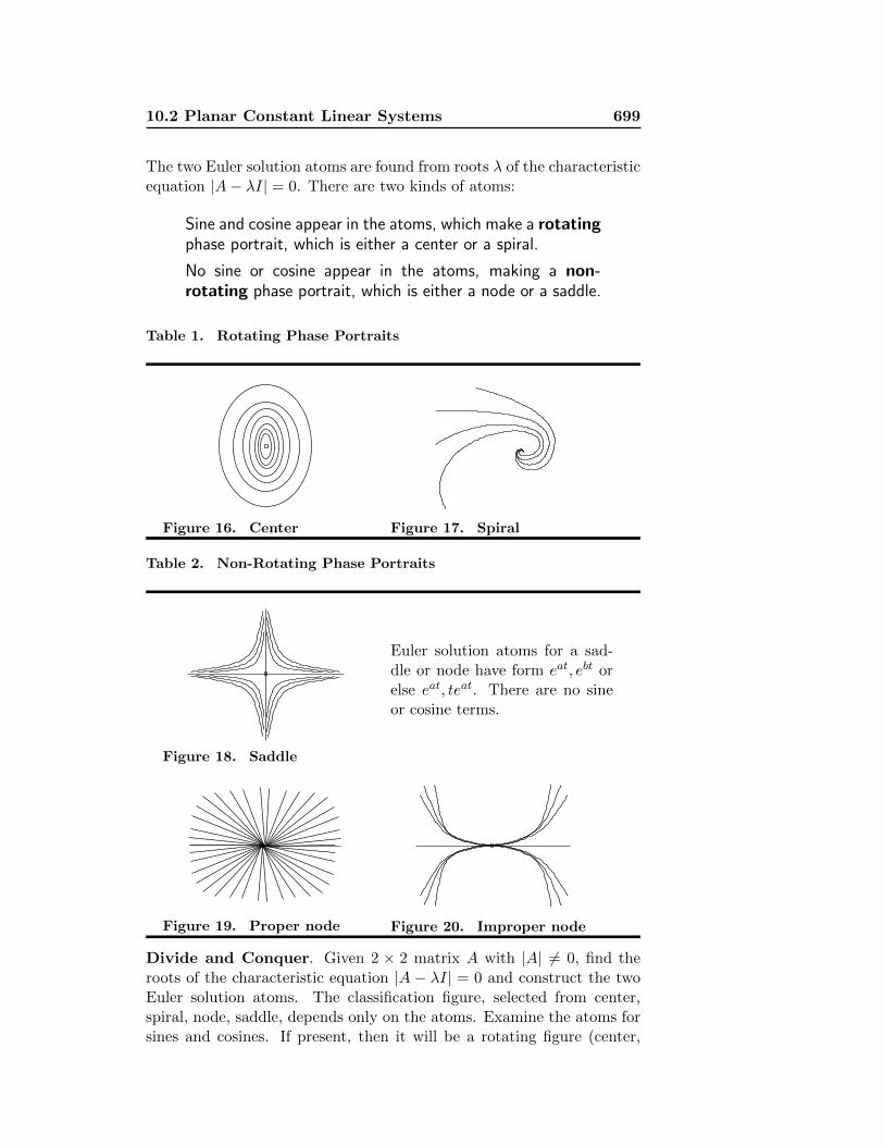
Sine and cosine appear in the atoms, which make a rotatingphase portrait, which is either a center or a spiral.
No sine or cosine appear in the atoms, making a non-rotating phase portrait, which is either a node or a saddle.
Table 1. Rotating Phase Portraits
Figure 16. Center Figure 17. Spiral
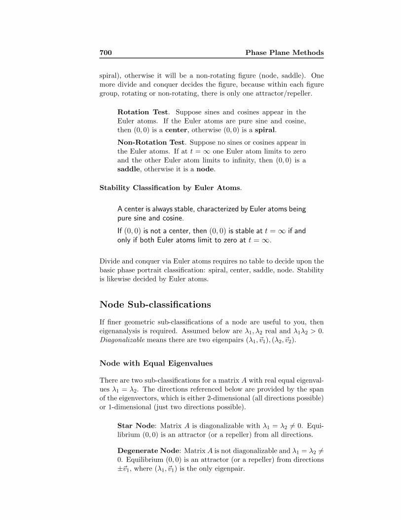
Table 2. Non-Rotating Phase Portraits
Figure 18. Saddle
Euler solution atoms for a sad-dle or node have form eat, ebt orelse eat, teat. There are no sineor cosine terms.
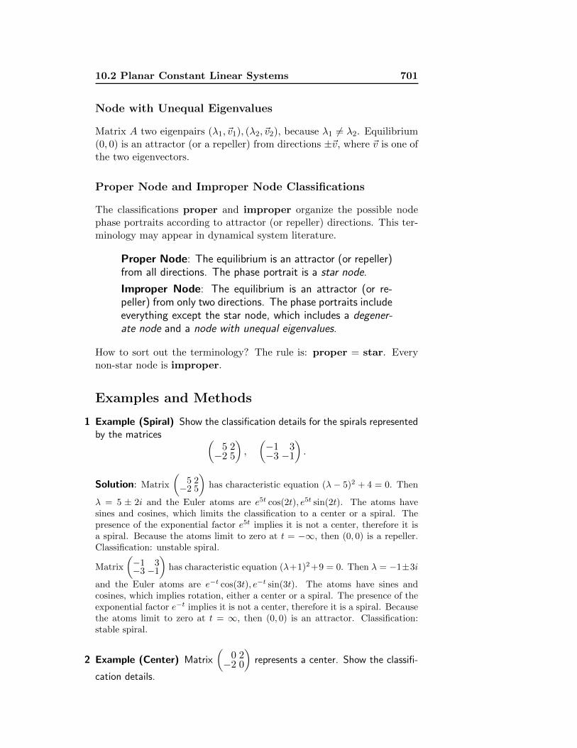
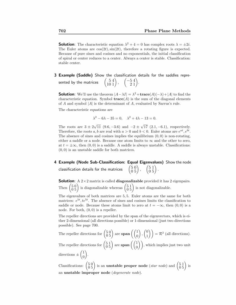
Figure 19. Proper node Figure 20. Improper node
Divide and Conquer. Given 2 × 2 matrix A with |A| 6= 0, find theroots of the characteristic equation |A − λI| = 0 and construct the twoEuler solution atoms. The classification figure, selected from center,spiral, node, saddle, depends only on the atoms. Examine the atoms forsines and cosines. If present, then it will be a rotating figure (center,
700 Phase Plane Methods
spiral), otherwise it will be a non-rotating figure (node, saddle). Onemore divide and conquer decides the figure, because within each figuregroup, rotating or non-rotating, there is only one attractor/repeller.
Rotation Test. Suppose sines and cosines appear in theEuler atoms. If the Euler atoms are pure sine and cosine,then (0, 0) is a center, otherwise (0, 0) is a spiral.
Non-Rotation Test. Suppose no sines or cosines appear inthe Euler atoms. If at t = ∞ one Euler atom limits to zeroand the other Euler atom limits to infinity, then (0, 0) is asaddle, otherwise it is a node.
Stability Classification by Euler Atoms.
A center is always stable, characterized by Euler atoms beingpure sine and cosine.
If (0, 0) is not a center, then (0, 0) is stable at t =∞ if andonly if both Euler atoms limit to zero at t =∞.
Divide and conquer via Euler atoms requires no table to decide upon thebasic phase portrait classification: spiral, center, saddle, node. Stabilityis likewise decided by Euler atoms.
Node Sub-classifications
If finer geometric sub-classifications of a node are useful to you, theneigenanalysis is required. Assumed below are λ1, λ2 real and λ1λ2 > 0.Diagonalizable means there are two eigenpairs (λ1, ~v1), (λ2, ~v2).
Node with Equal Eigenvalues
There are two sub-classifications for a matrix A with real equal eigenval-ues λ1 = λ2. The directions referenced below are provided by the spanof the eigenvectors, which is either 2-dimensional (all directions possible)or 1-dimensional (just two directions possible).
Star Node: Matrix A is diagonalizable with λ1 = λ2 6= 0. Equi-librium (0, 0) is an attractor (or a repeller) from all directions.
Degenerate Node: Matrix A is not diagonalizable and λ1 = λ2 6=0. Equilibrium (0, 0) is an attractor (or a repeller) from directions±~v1, where (λ1, ~v1) is the only eigenpair.
10.2 Planar Constant Linear Systems 701
Node with Unequal Eigenvalues
Matrix A two eigenpairs (λ1, ~v1), (λ2, ~v2), because λ1 6= λ2. Equilibrium(0, 0) is an attractor (or a repeller) from directions ±~v, where ~v is one ofthe two eigenvectors.
Proper Node and Improper Node Classifications
The classifications proper and improper organize the possible nodephase portraits according to attractor (or repeller) directions. This ter-minology may appear in dynamical system literature.
Proper Node: The equilibrium is an attractor (or repeller)from all directions. The phase portrait is a star node.
Improper Node: The equilibrium is an attractor (or re-peller) from only two directions. The phase portraits includeeverything except the star node, which includes a degener-ate node and a node with unequal eigenvalues.
How to sort out the terminology? The rule is: proper = star. Everynon-star node is improper.
Examples and Methods
1 Example (Spiral) Show the classification details for the spirals representedby the matrices (
5 2−2 5
),
(−1 3−3 −1
).
Solution: Matrix
(5 2−2 5
)has characteristic equation (λ− 5)2 + 4 = 0. Then
λ = 5 ± 2i and the Euler atoms are e5t cos(2t), e5t sin(2t). The atoms havesines and cosines, which limits the classification to a center or a spiral. Thepresence of the exponential factor e5t implies it is not a center, therefore it isa spiral. Because the atoms limit to zero at t = −∞, then (0, 0) is a repeller.Classification: unstable spiral.
Matrix
(−1 3−3 −1
)has characteristic equation (λ+1)2+9 = 0. Then λ = −1±3i
and the Euler atoms are e−t cos(3t), e−t sin(3t). The atoms have sines andcosines, which implies rotation, either a center or a spiral. The presence of theexponential factor e−t implies it is not a center, therefore it is a spiral. Becausethe atoms limit to zero at t = ∞, then (0, 0) is an attractor. Classification:stable spiral.
2 Example (Center) Matrix
(0 2−2 0
)represents a center. Show the classifi-
cation details.
702 Phase Plane Methods
Solution: The characteristic equation λ2 + 4 = 0 has complex roots λ = ±2i.The Euler atoms are cos(2t), sin(2t), therefore a rotating figure is expected.Because of pure sines and cosines and no exponentials, the initial classificationof spiral or center reduces to a center. Always a center is stable. Classification:stable center.
3 Example (Saddle) Show the classification details for the saddles repre-
sented by the matrices
(5 4
10 1
),
(−5 4
2 1
).
Solution: We’ll use the theorem |A−λI| = λ2+trace(A)(−λ)+ |A| to find thecharacteristic equation. Symbol trace(A) is the sum of the diagonal elementsof A and symbol |A| is the determinant of A, evaluated by Sarrus’s rule.
The characteristic equations are
λ2 − 6λ− 35 = 0, λ2 + 4λ− 13 = 0.
The roots are 3 ± 2√
11 (9.6,−3.6) and −2 ±√
17 (2.1,−6.1), respectively.Therefore, the roots a, b are real with a > 0 and b < 0. Euler atoms are eat, ebt.The absence of sines and cosines implies the equilibrium (0, 0) is non-rotating,either a saddle or a node. Because one atom limits to ∞ and the other to zero,at t = ±∞, then (0, 0) is a saddle. A saddle is always unstable. Classifications:(0, 0) is an unstable saddle for both matrices.
4 Example (Node Sub-Classification: Equal Eigenvalues) Show the node
classification details for the matrices
(5 00 5
),
(5 10 5
).
Solution: A 2×2 matrix is called diagonalizable provided it has 2 eigenpairs.
Then
(5 00 5
)is diagonalizable whereas
(5 10 5
)is not diagonalizable.
The eigenvalues of both matrices are 5, 5. Euler atoms are the same for bothmatrices: e5t, te5t. The absence of sines and cosines limits the classification tosaddle or node. Because these atoms limit to zero at t = −∞, then (0, 0) is anode. For both, (0, 0) is a repeller.
The repeller directions are provided by the span of the eigenvectors, which is ei-ther 2-dimensional (all directions possible) or 1-dimensional (just two directionspossible). See page 700.
The repeller directions for
(5 00 5
)are span
((10
),
(01
))= R2 (all directions).
The repeller directions for
(5 10 5
)are span
((10
)), which implies just two unit
directions ±(
10
).
Classifications:
(5 00 5
)is an unstable proper node (star node) and
(5 10 5
)is
an unstable improper node (degenerate node).
10.2 Planar Constant Linear Systems 703
5 Example (Node Sub-Classification: Unequal Eigenvalues) Show the node
classification details for the matrices
(−5 0
0 −7
),
(5 00 7
).
Solution: Both matrices are diagonal, hence each has two independent eigen-vectors. This example shows that diagonalizability by itself does not decide anode sub-classification.
Matrix
(−5 0
0 −7
)has unequal eigenvalues −5,−7 with Euler atoms e−5t, e−7t.
Absence of sines and cosines limits the classification to saddle or node. Theatoms have limit zero at t = ∞, which eliminates the saddle classification.Therefore, (0, 0) is an attractor. Classification: stable node.
For
(−5 0
0 −7
), an attractor orbit is tangent at t =∞ to ±~v1, where ~v1 =
(10
)is a unit eigenvector for λ1 = −5.
Matrix
(5 00 7
)has unequal eigenvalues 5, 7 with Euler atoms e5t, e7t. Absence
of sines and cosines limits the classification to saddle or node. The atoms havelimit zero at t = −∞, which eliminates the saddle classification. Therefore,(0, 0) is a repeller. Classification: unstable node.
For
(5 00 7
), a repeller orbit is tangent at t = ∞ to ±~v2, where ~v2 =
(01
)is a
unit eigenvector for λ2 = 7.
Computer Phase Diagrams. In computer node plots for unequal eigenvalues,an eigenvector direction can be detected from limits at t = ±∞. Attractors willhave the eigenvector direction for eigenvalue λ with |λ| smallest. Repellers willhave the eigenvector direction for eigenvalue λ with |λ| largest.
Exercises 10.2
Planar Constant Linear Systems.
1. (Picard’s Theorem) Explainwhy planar solutions don’t cross,by appeal to Picard’s existence-uniqueness theorem for d
dt~u=A~u.
2. (Equilibria) System ddt~u = A~u al-
ways has solution ~u(t) = ~0, so thereis always one equilibrium point.Give an example of a matrix Afor which there are infinitely manyequilibria.
Putzer’s Formula.
3. (Cayley-Hamilton) Define matri-
ces I =
(1 00 1
), 0 =
(0 00 0
). Given
matrix A =
(a bc d
), expand left and
right sides to verify the Cayley-Hamilton identityA2−(c+ d)A+ (ad−bc)I = 0.
4. (Complex Roots) Verify thePutzer solution ~u = Φ(t)~u(0)of ~u′ = A~u for complex rootsλ1 = λ2 = a + bi, b > 0, whereΦ(t) is
eat(
cos(bt) I + (A− aI)sin(bt)
b
).
5. (Distinct Eigenvalues) Solve
d
dt~u =
(−1 1
0 2
)~u.
6. (Real Equal Eigenvalues) Solve
d
dt~u =
(6 −44 −2
)~u.
704 Phase Plane Methods
7. (Complex Eigenvalues) Solve
d
dt~u =
(2 3−3 2
)~u.
Continuity and Redundancy.
8. (Real Equal Eigenvalues) Showthat limiting λ2 → λ1 in thePutzer formula for distinct eigen-values gives Putzer’s formula forreal equal eigenvalues.
9. (Complex Eigenvalues) Assumeλ1 = λ2 = a+ ib with b > 0. ThenPutzer’s first formula holds. Showthe third formula details for Φ(t):
eat(
cos(bt) I + (A− aI)sin(bt)
b
).
Illustrations.
10. (Distinct Eigenvalues) Show thedetails for the solution of
d
dt~u =
(−1 3−6 8
)~u.
11. (Complex Eigenvalues) Show thedetails for the solution of
d
dt~u =
(2 5−5 2
)~u.
Isolated Equilibria.
12. (Determinant Expansion) Verifythat |A− λI| equals
λ2 − (λ1 + λ2)λ+ λ1λ2.
13. (Infinitely Many Equilibria) Ex-plain why A~u = ~0 has infinitelymany solutions when det(A) = 0.
Classification of Equilibria.
14. (Rotating Figures) When sinesand cosines appear in the Euleratoms, the phase portrait at (0, 0)rotates around the origin. Explainprecisely why this is true.
15. (Non-Rotating Figures) Whensines and cosines do not appear inthe Euler atoms, the phase portraitat (0, 0) has no rotation. Give aprecise explanation.
Attractor and Repeller.
16. (Classification) Which of spiral,center, saddle, node can be an at-tractor or a repeller?
17. (Attractor) Prove that (0, 0) is anattractor if and only if the Euleratoms have limit zero at t =∞.
18. (Repeller) Prove that (0, 0) is arepeller if and only if the Euleratoms have limit zero at t = −∞.
19. (Center) A center is neither an at-tractor nor a repeller. Explain, us-ing Euler atoms.
Phase Portrait Linear. Show theclassification details for spiral, cen-ter, saddle, proper node, impropernode. Include a drawing which identi-fies eigenvector directions, where suchinformation applies.
20. (Spiral)
ddtx = 2x+ 3y,ddty = −3x+ 2y.
21. (Center)
ddtx = 3y,ddty = −3x.
22. (Saddle)
ddtx = 3x,ddty = −5y.
23. (Proper Node)
ddtx = 2x,ddty = 2y.
24. (Improper Node: Degenerate)
ddtx = 2x+ y,ddty = 2y.
25. (Improper Node: λ1 6= λ2)
ddtx = 2x+ y,ddty = 3y.
10.3 Planar Almost Linear Systems 705
10.3 Planar Almost Linear Systems
A nonlinear planar autonomous system ddt~u(t) = ~F (~u(t)) is called almost
linear at equilibrium point ~u = ~u0 if
~F (~u) = A(~u− ~u0) + ~G(~u),
lim‖~u−~u0‖→0
‖~G(~u)‖‖~u− ~u0‖
= 0.
The function ~G has the same smoothness as ~F . We investigate thepossibility that a local phase portrait at ~u = ~u0 for the nonlinear systemddt~u(t) = ~F (~u(t)) is graphically identical to the one for the linear system~v′(t) = A~v(t) at ~v = 0.
The results will apply to all isolated equilibria of ddt~u(t) = ~F (~u(t)).
This is accomplished by expanding F in a Taylor series about each equi-librium point, which implies that the ideas are applicable to differentchoices of A and G, depending upon which equilibrium point ~u0 wasconsidered.
Define the Jacobian matrix of ~F =
(fg
)at equilibrium point ~u0 by
the formula
J =
(fx fygx gy
).
Taylor’s theorem for functions of two variables says that
~F (~u) = J(~u− ~u0) + ~G(~u)
where ~G(~u)/‖~u−~u0‖ → 0 as ‖~u−~u0‖ → 0. Therefore, for ~F continuouslydifferentiable, we may always take A = J to obtain from the almost linearsystem d
dt~u(t) = ~F (~u(t)) its linearization ddt~v(t) = A~v(t).
Phase Portrait of an Almost Linear System
For planar almost linear systems ddt~u(t) = ~F (~u(t)), phase portraits have
been studied extensively, by Poincare-Bendixson and a long list of re-searchers. It is known that only a finite number of local phase portraitsare possible near each isolated equilibrium point of the nonlinear system,the library of figures being identical to those possibilities for a linear sys-tem ~v′(t) = A~v(t). A precise statement, without proof, appears below.
Theorem 4 (Paste Theorem: Almost Linear System Phase Portrait)Let the planar almost linear system d
dt~u(t) = ~F (~u(t)) be given with ~F (~u) =
A(~u − ~u0) + ~G(~u) near the isolated equilibrium point ~u0 (an isolated rootof ~F (~u0) = ~0 with |A| 6= 0). Let λ1, λ2 be the roots of det(A − λI) = 0.Then:
706 Phase Plane Methods
1. If λ1 = λ2, then the equilibrium ~u0 of the nonlinear system ddt~u(t) =
~F (~u(t)) is either a node or a spiral. The equilibrium ~u0 is an asymp-totically stable attractor if λ1 < 0 and it is a repeller if λ1 > 0. Inshort, the nonlinear system inherits stability from the linear system.
2. If λ1 = λ2 = ib with b > 0, then the equilibrium ~u0 of the nonlinearsystem d
dt~u(t) = ~F (~u(t)) is either a center or a spiral. The stabilityof the equilibrium ~u0 cannot be predicted from properties of A.
3. In all other cases, the isolated equilibrium ~u0 has graphically the samelocal phase portrait as the associated linear system d
dt~v(t) = A~v(t) at
~v = ~0. In particular, local phase portraits of a saddle, spiral or nodecan be graphed from the linear system. The nonlinear system inheritslocally the linearized system properties of stability and instability.
Classification of Almost Linear Equilibria
A system ddt~u(t) = A (~u(t)− ~u0) + ~G(~u(t)) has a local phase portrait
determined by the linear system ~v′(t) = A~v(t), except in the case whenthe roots λ1, λ2 of the characteristic equation det(A−λI) = 0 are equalor purely imaginary (see Theorem 4). To summarize:
Table 3. Equilibria classification for almost linear systems
Eigenvalues of A Nonlinear Classification
λ1 < 0 < λ2 Unstable saddleλ1 < λ2 < 0 Stable improper nodeλ1 > λ2 > 0 Unstable improper nodeλ1 = λ2 < 0 Stable node or spiralλ1 = λ2 > 0 Unstable node or spiralλ1 = λ2 = a+ ib, a < 0, b > 0 Stable spiralλ1 = λ2 = a+ ib, a > 0, b > 0 Unstable spiralλ1 = λ2 = ib, b > 0 Stable or unstable, center or spiral
Almost Linear Equilibria Geometry
Applied literature may refer to an equilibrium point ~u0 of a nonlinearsystem d
dt~u(t) = ~F (~u(t)) as a spiral, center, saddle or node. The geome-try of these classifications is explained below.
Spiral. To describe a nonlinear spiral, we require that an orbit start-ing on a given ray emanating from the equilibrium point mustintersect that ray in infinitely many distinct points on (−∞,∞).
10.3 Planar Almost Linear Systems 707
Intutition. Basic understanding of a nonlinear spiral is ob-tained from a linear example, e.g.,
d
dt~u(t) =
(−1 2−2 −1
)~u(t).
An orbit has component solutions
x(t) = e−t(A cos 2t+B sin 2t), y(t) = e−t(−A sin 2t+B cos 2t)
which oscillate infinity often on (−∞,∞), rotating around equilib-rium point (0, 0) with amplitude Ce−t, for some constant C > 0.
Center. Local orbits are periodic solutions. Each local orbit is a closedcurve which forms a planar region with boundary, having the equi-librium point interior. As the periodic orbits shrink, the planar re-gion also shrinks, limiting as a planar set to the equilibrium point.Drawings often portray the periodic orbit as a convex figure, butthis is not correct, in general, because the periodic orbit can haveany shape. In particular, the linearized system may have phaseportrait consisting of concentric circles, but the nonlinear phaseportrait has no such exact geometric structure.
Saddle. The term implies that locally the phase portrait looks like a lin-ear saddle. In nonlinear phase portraits, the straight lines to whichorbits are asymptotic appear to be curves instead. These curves arecalled separatrices, which are generally unions of certain orbitsand equilibria.
Node. Each orbit starting near the equilibrium is expected to limit tothe equilibrium at either t = ∞ (stable attractor) or t = −∞(unstable repeller), in a fashion asymptotic to a direction ~v. Theterminology applies when the linearized system is a proper node(a.k.a. star node), in which case there is an orbit asymptotic to ~vfor every direction ~v. If there is only one direction ~v possible, or allorbits are asymptotic to just one separatrix, then the equilibriumis classified as an improper node. The term degenerate nodeapplies to a subclass of improper nodes – see Example 4, page 702.
Pasting Figures to make a Nonlinear Phase Portrait
The plan provided by the theorem is to paste a library source figure,one of spiral, center, saddle or node, overlaying (0, 0) in the source figureatop equilibrium point ~u = ~u0 in the nonlinear phase portrait. Someobservations follow, about what works and what fails.
1. The local paste is valid to graphical resolution near ~u = ~u0, andinvalid far away from the equilibrium point.
708 Phase Plane Methods
2. The pasted figure can mutate into a spiral, if the source figure iseither a center, or else a node with λ1 = λ2. Otherwise, saddle,spiral and node locally paste into saddle, spiral, node.
3. Stability of the source figure is inherited by the nonlinear portrait,except when the source is a center. In this one exceptional case,no stability conclusion can be drawn. However, an attractor orrepeller source figure always pastes into an attractor or a repeller.
Examples and Methods
6 Example (Compute Isolated Equilibria) Find all equilibria for the non-linear system
x′(t) = x(t) + y(t), y′(t) = 1− x2(t).
Solution: Equilibria are constant solutions, obtained formally by setting x′ =y′ = 0 in the two differential equations x′ = x+ y, y′ = 1− x2. Then solve forconstants x, y. The details:
Set x′ = 0 0 = x+ y
Set y′ = 0 0 = 1− x2
Solve for x, y x = ±1, y = −x.
Equilibria (1,−1) and (−1, 1)
7 Example (Linearization at Equilibria) Find the two linearizations at equi-libria (1,−1), (−1, 1) for the nonlinear system
x′(t) = x(t) + y(t), y′(t) = 1− x2(t).
Solution: The system of differential equations is written with function notationin the form x′ = f(x, y), y′ = g(x, y). Then
f(x, y) = x+ y, g(x, y) = 1− x2.
The Jacobian matrix
J(x, y) =
(fx fygx gy
)is computed with symbols x, y, f, g as follows.
Partial derivative fx(x, y): fx = ∂x(x+ y) = 1 + 0 = 1
Partial derivative gx(x, y): gx = ∂x(1− x2) = 0− 2x = −2x
Partial derivative fy(x, y): fy = ∂y(x+ y) = 0 + 1 = 1
Partial derivative gy(x, y): gy = ∂y(1− x2) = 0− 0 = 0
10.3 Planar Almost Linear Systems 709
Then
J(x, y) =
(fx fygx gy
)=
(1 1
−2x 0
).
The symbols x, y are used for the two substitutions: x = 1, y = −1 and x =−1, y = 1.
J(1,−1) =
(1 1−2 0
), J(−1, 1) =
(1 12 0
).
The two linearized problems are
d
dt~u =
(1 1−2 0
)~u,
d
dt~u =
(1 12 0
)~u.
8 Example (Classification of Linearized Problems) Classify the two linearproblems
d
dt~u =
(1 1−2 0
)~u,
d
dt~u =
(1 12 0
)~u.
Solution:
The answers:
(1 1−2 0
)is an unstable spiral;
(1 12 0
)is an unstable saddle.
The two characteristic equations are λ2 − λ + 2 = 0 and λ2 + λ + 2 = 0 with
roots, respectively, 12 ± i
√72 and 2,−1. According to the classification theory,
page 696, the equilibrium (0, 0) is respectively an unstable spiral or an unstablesaddle.
9 Example (Pasting Library Linear Portraits onto Nonlinear Portraits)Classify equilibria (1,−1), (−1, 1) for the nonlinear system
x′(t) = x(t) + y(t), y′(t) = 1− x2(t),
as nonlinear spiral, center, saddle or node. Paste the linear portraits forJ(−1, 1), J(1,−1) onto the nonlinear direction field portrait, when possible.
Solution: Classifications: (−1, 1) is a nonlinear unstable saddle; (1,−1) is anonlinear unstable spiral.
Previous examples show that for the linearized problems, (−1, 1) is an unsta-ble saddle and (−1, 1) is an unstable spiral. Theorem 4 applies to concludethat the two linear phase portraits directly transfer onto the nonlinear phaseportrait. This means that (0, 0) in each source figure can be pasted atop thecorresponding equilibrium point in the nonlinear system, the pasted figure validlocally.
Computer phase portraits show the two pasted library figures with automaticfine tuning. Especially, the saddle will be tuned, because a library source figureusually has asymptotes parallel to the coordinate axes, whereas the computergraphic will show tuned asymptotes in eigenvector directions.
710 Phase Plane Methods
x
y
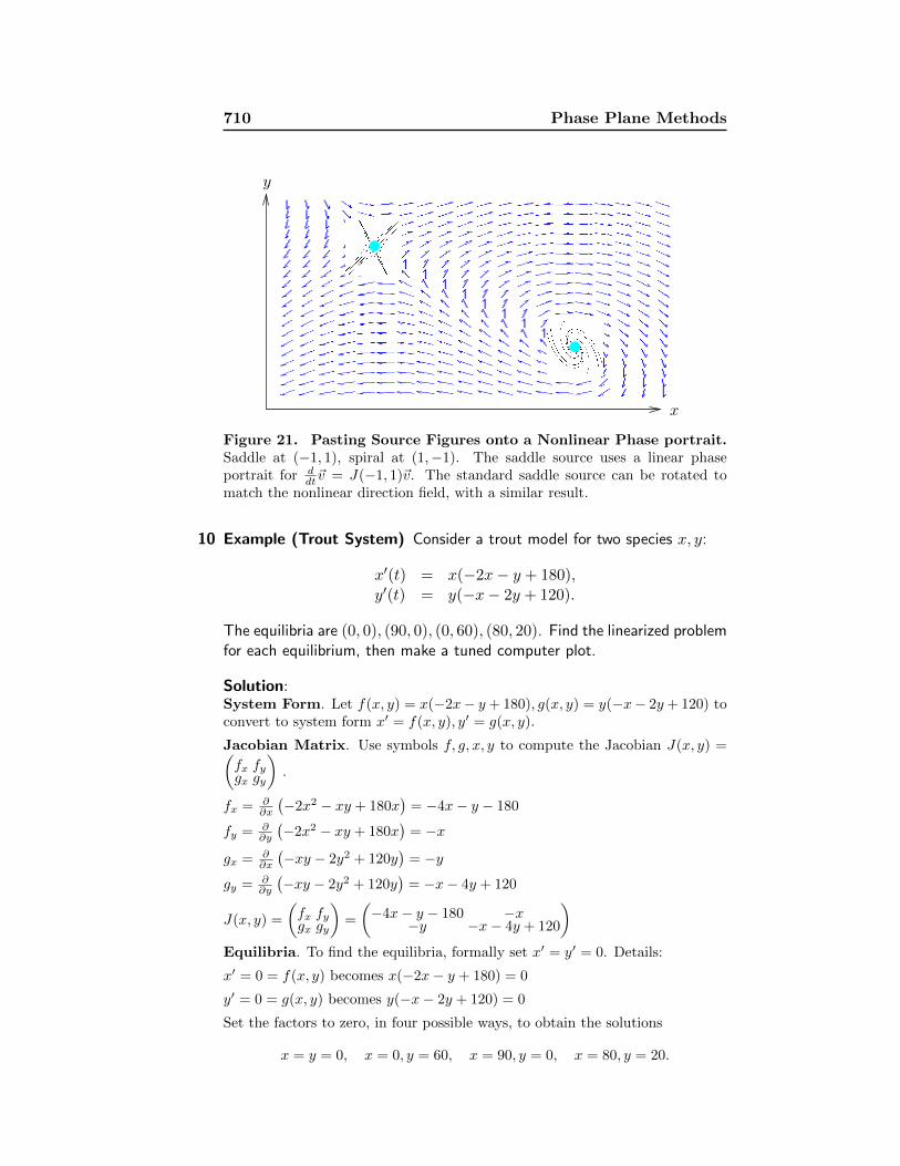
Figure 21. Pasting Source Figures onto a Nonlinear Phase portrait.Saddle at (−1, 1), spiral at (1,−1). The saddle source uses a linear phaseportrait for d
dt~v = J(−1, 1)~v. The standard saddle source can be rotated tomatch the nonlinear direction field, with a similar result.
10 Example (Trout System) Consider a trout model for two species x, y:
x′(t) = x(−2x− y + 180),y′(t) = y(−x− 2y + 120).
The equilibria are (0, 0), (90, 0), (0, 60), (80, 20). Find the linearized problemfor each equilibrium, then make a tuned computer plot.
Solution:System Form. Let f(x, y) = x(−2x− y + 180), g(x, y) = y(−x− 2y + 120) toconvert to system form x′ = f(x, y), y′ = g(x, y).
Jacobian Matrix. Use symbols f, g, x, y to compute the Jacobian J(x, y) =(fx fygx gy
).
fx = ∂∂x
(−2x2 − xy + 180x
)= −4x− y − 180
fy = ∂∂y
(−2x2 − xy + 180x
)= −x
gx = ∂∂x
(−xy − 2y2 + 120y
)= −y
gy = ∂∂y
(−xy − 2y2 + 120y
)= −x− 4y + 120
J(x, y) =
(fx fygx gy
)=
(−4x− y − 180 −x
−y −x− 4y + 120
)Equilibria. To find the equilibria, formally set x′ = y′ = 0. Details:
x′ = 0 = f(x, y) becomes x(−2x− y + 180) = 0
y′ = 0 = g(x, y) becomes y(−x− 2y + 120) = 0
Set the factors to zero, in four possible ways, to obtain the solutions
x = y = 0, x = 0, y = 60, x = 90, y = 0, x = 80, y = 20.
10.3 Planar Almost Linear Systems 711
Linearized Differential Equations. The linear problems ddt~u = J(x0, y0)~u
at equilibria (0, 0), (0, 60), (90, 0), (80, 20) are created from the four Jacobianmatrices
J(0, 0) =
(−180 0
0 120
), J(0, 60) =
(120 0−60 −120
),
J(90, 0) =
(−180 −90
0 30
), J(80, 20) =
(−160 −80−20 −40
).
Eigenvalues. Answers for the four matrices are respectively 120, 180, 120,−120,30,−180, −27.89,−172.11.
Linear Classifications. Because there are no complex eigenvalues, then thepossible linear phase portraits are either saddle or node. Checking limits ofEuler atoms at t =∞ reveals the classifications unstable node, saddle, saddle,stable node. No equal eigenvalues implies both nodes are improper.
Paste Theorem. All linear source figures paste directly onto the nonlinearphase portrait with stability properties inherited. See Theorem 4.
Eigenvectors help understanding of the phase portrait. In all four figures,asymptote directions are along an eigenvector. For instance, at (80, 20) the
two eigenvector directions are ~v1 =
(−0.6
1
), ~v2 =
(6.6
1
).
y
x
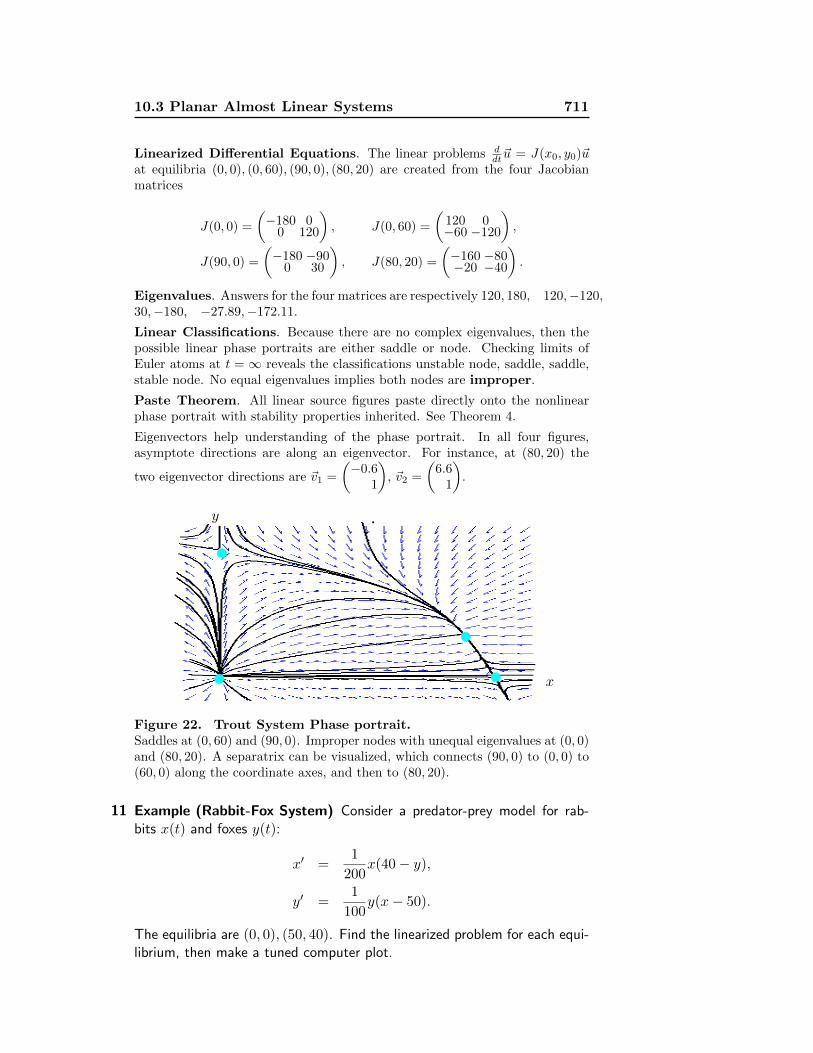
Figure 22. Trout System Phase portrait.Saddles at (0, 60) and (90, 0). Improper nodes with unequal eigenvalues at (0, 0)and (80, 20). A separatrix can be visualized, which connects (90, 0) to (0, 0) to(60, 0) along the coordinate axes, and then to (80, 20).
11 Example (Rabbit-Fox System) Consider a predator-prey model for rab-bits x(t) and foxes y(t):
x′ =1
200x(40− y),
y′ =1
100y(x− 50).
The equilibria are (0, 0), (50, 40). Find the linearized problem for each equi-librium, then make a tuned computer plot.
712 Phase Plane Methods
Solution:System Form. Let f(x, y) = 1
200x(40 − y), g(x, y) = 1100y(x − 50) to convert
to system form x′ = f(x, y), y′ = g(x, y).
Jacobian Matrix. Symbols f, g, x, y are used to compute the Jacobian J(x, y) =(fx fygx gy
).
fx = ∂∂x (x/5− xy/200) = 1/5− y/200
fy = ∂∂y (x/5− xy/200) = −x/200
gx = ∂∂x (−y/2 + xy/100) = y/100
gy = ∂∂y (−y/2 + xy/100) = −x− 4y + 120
J(x, y) =
(fx fygx gy
)=
(−4x− y − 180 −x
−y −x− 4y + 120
)Equilibria. To find the equilibria (0, 0), (50, 40), formally set x′ = y′ = 0.Details:
0 = f(x, y) becomes 1200x(40− y) = 0
0 = g(x, y) becomes 1100y(x− 50) = 0
The solutions are x = y = 0 or else x = 50, y = 40.
Linearized Differential Equations. The linear problems ddt~u = J(x0, y0)~u
at equilibria (0, 0), (50, 40) are created from the two Jacobian matrices
J(0, 0) =
(15 00 − 1
2
), J(50, 40) =
(0 − 1
425 0
).
Eigenvalues. The answers are 15 ,−
12 and ±i/
√10, respectively.
Linear Classifications. Complex eigenvalues imply linear phase portraits ofeither center or node. Checking Euler atoms reveals the classification center at(50, 40). Real unequal eigenvalues at (0, 0) implies a saddle or node. Checkinglimits of the Euler atoms at t =∞ implies (0, 0) is a saddle. Both linear sourcefigures are stable.
Paste Theorem. The linear saddle source figure for (0, 0) pastes directly ontothe nonlinear phase portrait at (0, 0) with stability properties inherited. Thelinear center source figure for (50, 40) pastes into a center or a spiral at (50, 40).The paste stability or instability is not decided. See Theorem 4.
The easiest path to deciding the nonlinear portrait at (50, 40) is a computerphase portrait, which shows a center structure.
Eigenvectors help understanding of the phase portrait. At (0, 0) the two eigen-
vector directions are ~v1 =
(10
), ~v2 =
(01
).
10.3 Planar Almost Linear Systems 713
y
x
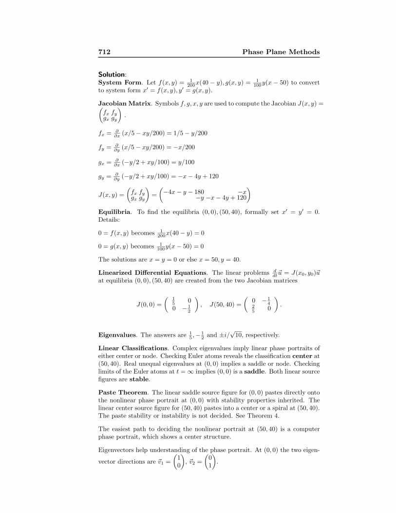
Figure 23. Rabbit-Fox System Phase portrait.Eigenvector directions for the saddle at (0, 0) are parallel to the coordinate axes.The linear center from J(50, 40) happens to transfer to a nonlinear center at(50, 40).
Exercises 10.3
Almost Linear Systems. Find allequilibria (x0, y0) of the given nonlin-ear system. Then compute the Jaco-bian matrix A = J(x0, y0) for eachequilibria.
1. (Spiral and Saddle)
ddtx = x+ 2y,ddty = 1− x2.
2. (Saddle and Two Spirals)
ddtx = x− 3y + 2xy,ddty = 4x− 6y − xy − x2.
3. (Spiral, Saddle)
ddtx = 3x− 2y − x2 − y2,ddty = 2x− y.
4. (Center and Three Saddles)
ddtx = x− y + x2 − y2,ddty = 2x− y − xy.
5. (Proper Node and Three Sad-
dles)
ddtx = x− y + x2 − y2,ddty = y − xy.
6. (Improper Degenerate Node,
Spiral and Two Saddles)
ddtx = x− y + x3 + y3,ddty = y + 3xy.
7. (Improper Node and a Saddle)
ddtx = x− y + x3,ddty = 2y + 3xy.
8. (Proper Node and a Saddle)
ddtx = 2x+ y3,ddty = 2y + 3xy.
Phase Portrait Almost Linear. Lin-ear library phase portraits can be lo-cally pasted atop the equilibria of analmost linear system, with limitations.Apply the theory for the following ex-amples. Complete the phase diagramby computer, thereby resolving thepossible mutation of a center or nodeinto a spiral. Label eigenvector direc-tions, where it makes sense.
9. (Center and Three Saddles)
ddtx = x− y + x2 − y2,ddty = 2x− y − xy.
714 Phase Plane Methods
10. (Proper Node and 3 Saddles)
ddtx = x− y + x2 − y2,ddty = y − xy.
11. (Improper Degenerate Node,
Spiral and Two Saddles)
ddtx = x− y + x3 + y3,ddty = y + 3xy.
12. (Improper Node and a Saddle)
ddtx = x− y + x3,ddty = 2y + 3xy.
13. (Proper Node and a Saddle)
ddtx = 2x+ y3,ddty = 2y + 3xy.
Classification of Almost LinearEquilibria. With computer assist, findand classify the nonlinear equilibria.
14. (Co-existing Species)
x′(t) = x(t)(24− 2x(t)− y(t)),y′(t) = y(t)(30− 2y(t)− x(t)).
15. (Doomsday-Extinction)
x′(t) = x(t)(x(t)− y(t)− 4),y′(t) = y(t)(x(t) + y(t)− 8).
Almost Linear Geometry. A separa-trix is a union of curves and equilibriawith orbits limiting to it. With com-puter assist, make a plot of threadedcurves which identify one or more sep-aratrices near the equilibrium.
16. (Saddle (−1, 1))
ddtx = x+ y,ddty = 1− x2.
17. (Saddle (−1/5,−2/5))
ddtx = 3x− 2y − x2 − y2,ddty = 2x− y.
18. (Saddle (−2/3, 3√
4/3))
ddtx = 2x+ y3,ddty = 2y + 3xy.
19. (Degenerate Improper Node)
ddtx = x− y + x3 + y3,ddty = y + 3xy, at (0, 0).
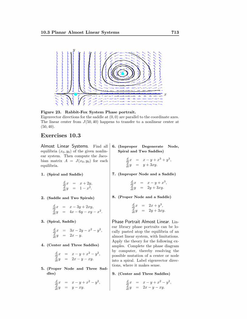
Rayleigh and van der Pol. Each ex-ample below has a unique periodic or-bit surrounding an equilibrium pointthat is the limit at t = ∞ of anyother orbit. Verify the spiral repellerat (0, 0) in the attached figure, fromthe linearized problem at (0, 0) andPaste Theorem 4. Create phase por-traits with computer assist for the lin-ear and nonlinear problems.
20. (Lord Rayleigh 1877, Clarinet
Reed Model)
ddtx = y,
ddty = −x+ y − y3.
Figure 24. Clarinet Reed.
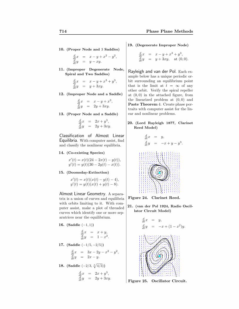
21. (van der Pol 1924, Radio Oscil-
lator Circuit Model)
ddtx = y,
ddty = −x+ (1− x2)y.
Figure 25. Oscillator Circuit.
10.4 Biological Models 715
10.4 Biological Models
Studied here are predator-prey models and competition modelsfor two populations. Assumed as background from population biol-ogy are the one-dimensional Malthusian model d
dtP = kP and the one-
dimensional Verhulst model ddtP = (a− bP )P .
Predator-Prey Models
One species called the predator feeds on the other species called theprey. The prey feeds on some constantly available food supply, e.g.,rabbits eat plants and foxes eat rabbits.
Credited with the classical predator-prey model is the Italian mathe-matician Vito Volterra (1860-1940), who worked on cyclic variationsin shark and prey-fish populations in the Adriatic sea. The followingbiological assumptions apply to model a predator-prey system.
Malthusian Growth The prey population grows according to thegrowth equation x′(t) = a x(t), a > 0, in theabsence of predators.
Malthusian Decay The predator population decays according to thedecay equation y′(t) = −b y(t), b > 0, in theabsence of prey.
Chance Encounters The prey decrease population at a rate −pxy,p > 0, due to chance encounters of predatorsy with prey x. Predators increase populationdue to these chance interactions at a rate qxy,q > 0.
The interaction terms qxy and −pxy are justified by arguing that thefrequency of chance encounters is proportional to the product xy. Bi-ologists explain the proportionality by saying that doubling either pop-ulation should double the frequency of chance encounters. Adding theMalthusian rates and the chance encounter rates gives the Volterrapredator-prey system1
x′(t) = (a− p y(t))x(t),y′(t) = (q x(t)− b)y(t).
(1)
The differential equations are displayed in this form in order to emphasizethat each of x(t) and y(t) satisfy a scalar first order differential equa-tion u′(t) = r(t)u(t) in which the rate function r(t) depends on time.
1The system is written with prey x and predator y. Alphabetical order predator-prey would have y first and then x.
716 Phase Plane Methods
For initial population sizes near zero, the two differential equations be-have very much like the Malthusian growth model u′(t) = a u(t) and theMalthusian decay model u′(t) = −b u(t). This basic growth/decay prop-erty allows us to identify the predator variable y, or the prey variablex, regardless of the order in which the differential equations are written.As viewed from Malthus’ law u′ = ru, the prey population has growthrate r = a− py which gets smaller as the number y of predators grows,resulting in fewer prey. Likewise, the predator population has decay rater = −b + qx, which gets larger as the number x of prey grows, causingincreased predation. These are the basic ideas of Verhulst, applied tothe individual populations x and y.
System Variables
The system of two differential equations (1) can be written as a planarvector autonomous system
d
dt~u = ~F (~u)
where ~F is defined by
~F (~u) =
((a− py)x(qx− b)y)
), ~u =
(xy
).(2)
The vector function ~F is everywhere defined and continuously differen-tiable. The Picard–Lindelof theorem provides existence-uniqueness.
A planar vector autonomous system ddt~u = ~F (~u) can be written in stan-
dard scalar system form
x′ = f(x, y), y′ = g(x, y)
by providing definitions for f(x, y) and g(x, y). For predator-prey system(1), the definitions are
f(x, y) = (a− p y)x, g(x, y) = (q x− b)y.
Equilibria
The equilibrium points ~u =
(x0y0
)satisfy ~F (~u) = ~0. For predator-prey
system (1), the equilibria are (0, 0) and (b/q, a/p), found by solving forx0, y0 in the equations (a− p y0)x0 = 0, (q x0 − b)y0 = 0.
10.4 Biological Models 717
Linearized Predator-Prey System
The linearized system at equilibrium (x0, y0) is the vector-matrix systemddt~v(t) = A~v(t), where A is the Jacobian matrix J(x, y) evaluated at pointx = x0, y = y0, briefly A = J(x0, y0). In terms of system variables2,
J(x0, y0) =
(fx(x0, y0) fy(x0, y0)gx(x0, y0) gy(x0, y0)
).
For the predator-prey system, we start by computing
fx =∂
∂x(a x− p xy) = a− p y, fy =
∂
∂y(a x− p xy) = 0− p x,
gx =∂
∂x(q xy − b y) = q y − 0, gy =
∂
∂y(q xy − b y) = q x− b.
The Jacobian matrix is given explicitly by
J(x, y) =
(fx fygx gy
)=
(a− p y −p xq y q x− b
).(3)
The matrix J is evaluated at equilibrium points (0, 0), (b/q, a/p) to ob-tain the 2× 2 matrices for the linearized systems:
J(0, 0) =
(a 00 −b
), J(b/q, a/p) =
(0 −bp/q
aq/p 0
).
The linearized systems ~v′(t) = A~v(t) are:
Equilibrium (0, 0) ddt~u(t) =
(a 00 −b
)~u(t)
Equilibrium (b/q, a/p) ddt~u(t) =
(0 −bp/q
aq/p 0
)~u(t)
Saddle J(0, 0). Matrix
(a 00 −b
)has unequal real eigenvalues a,−b and
associated Euler atoms eat, e−bt. No rotation implies a saddle or node,but limits at infinity imply a linear saddle. The Paste Theorem im-plies system d
dt~u(t) = ~F (~u(t)) has a saddle at equilibrium (0, 0).
Center J(b/q, a/p). Matrix
(0 −bp/q
aq/p 0
)has complex conjugate eigen-
values ±i√ab and associated Euler atoms cos(t
√ab), cos(t
√ab). Pure
rotation (no exponential factor) implies a linear center. The PasteTheorem implies system d
dt~u(t) = ~F (~u(t)) has either a center or a spi-ral at equilibrium (b/q, a/p).
Shown below in Theorem 5 is that the spiral case does not happen.The proof of Lemma 1 is in the exercises.
2Notation fx means ∂f/∂x, the calculus x-derivative with all other variables heldconstant.

718 Phase Plane Methods
Lemma 1 (Predator-Prey Implicit Solution)Let (x(t), y(t)) be an orbit of the predator-prey system (1) with x(0) > 0
and y(0) > 0. Then for some constant C,
a ln |y(t)|+ b ln |x(t)| − q x(t)− p y(t) = C.(4)
Theorem 5 (Spiral Case Eliminated)
Equilibrium (b/q, a/p) of predator-prey system (1) cannot be a spiral.
Proof: Assume the equilibrium (b/q, a/p) is a spiral point and some orbittouches the line x = b/q in points (b/q, u1), (b/q, u2) with u1 6= u2, u1 > a/p,u2 > a/p. Consider the energy function E(u) = a ln |u| − p u. Due to relation(4), E(u1) = E(u2) = E0, where E0 ≡ C + b − b ln |b/q|. By the Mean ValueTheorem of calculus, dE/du = 0 at some u between u1 and u2. This is acontradiction, because dE/du = (a−pu)/u is strictly negative for a/p < u <∞.Therefore, equilibrium (b/q, a/p) is not a spiral.
Rabbits and Foxes
An instance of predator-prey theory is a Volterra population model forx rabbits and y foxes given by the system of differential equations
x′(t) =1
250x(t)(40− y(t)),
y′(t) =1
50y(t)(x(t)− 60).
(5)
The equilibria of system (5) are (0, 0) and (60, 40). A phase portrait forsystem (5) appears in Figure 26.
The linearized system at (60, 40) is
x′(t) = − 6
25y(t),
y′(t) =4
5x(t).
This system has eigenvalues ±i√
24/125 and Euler atoms sin(t√
24/125),cos(t
√24/125), which have period 2π/
√24/125 ≈ 14.33934302. The
linear classification is a center.
The nonlinear classification at (60, 40) is then a center, because of Theo-rem 5. Intuition dictates that the period of smaller and smaller nonlinearorbits enclosing the equilibrium (60, 40) must approach a value that isapproximately 14.3.
The fluctuations in population size x(t) are measured graphically bythe maximum and minimum values of x in the phase portrait, or more
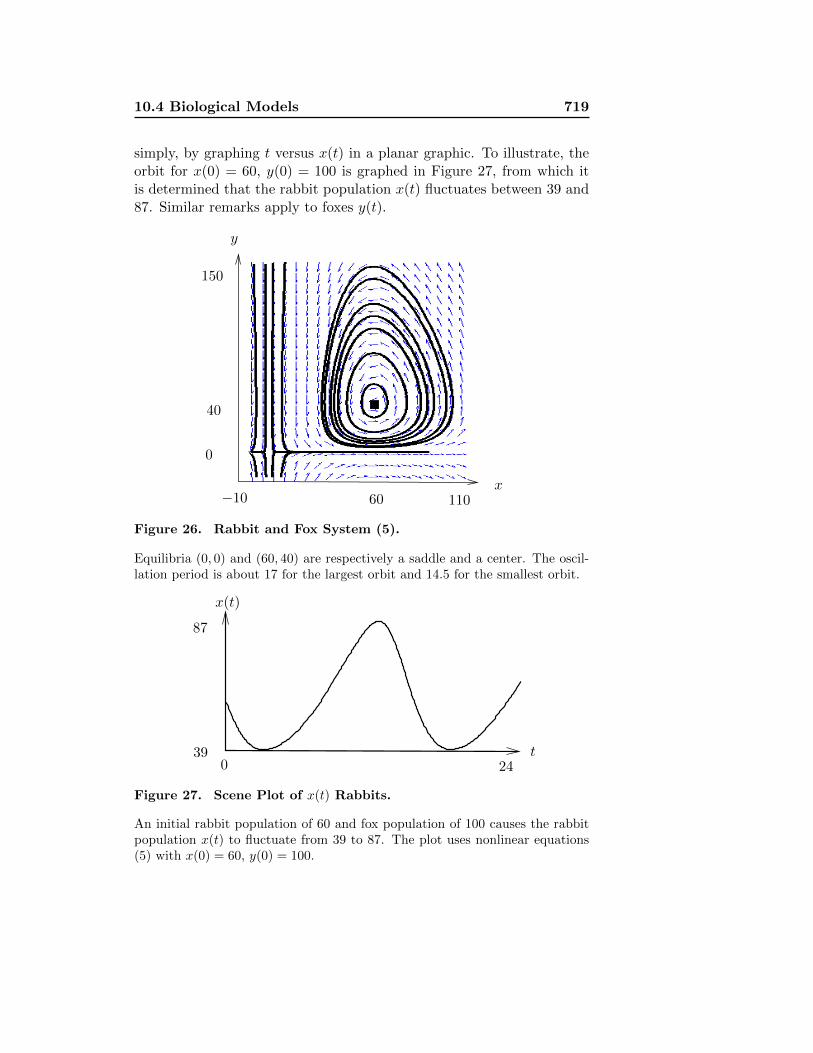
10.4 Biological Models 719
simply, by graphing t versus x(t) in a planar graphic. To illustrate, theorbit for x(0) = 60, y(0) = 100 is graphed in Figure 27, from which itis determined that the rabbit population x(t) fluctuates between 39 and87. Similar remarks apply to foxes y(t).
y
x
0
40
150
11060−10
Figure 26. Rabbit and Fox System (5).
Equilibria (0, 0) and (60, 40) are respectively a saddle and a center. The oscil-lation period is about 17 for the largest orbit and 14.5 for the smallest orbit.
24039
87
t
x(t)
Figure 27. Scene Plot of x(t) Rabbits.
An initial rabbit population of 60 and fox population of 100 causes the rabbitpopulation x(t) to fluctuate from 39 to 87. The plot uses nonlinear equations(5) with x(0) = 60, y(0) = 100.
720 Phase Plane Methods
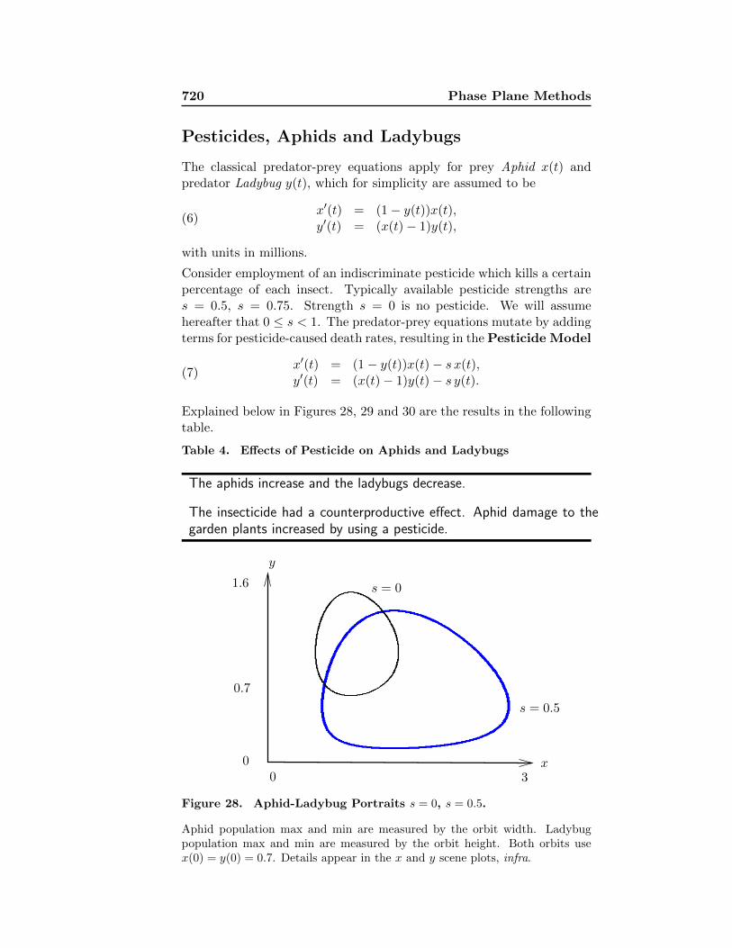
Pesticides, Aphids and Ladybugs
The classical predator-prey equations apply for prey Aphid x(t) andpredator Ladybug y(t), which for simplicity are assumed to be
x′(t) = (1− y(t))x(t),y′(t) = (x(t)− 1)y(t),
(6)
with units in millions.
Consider employment of an indiscriminate pesticide which kills a certainpercentage of each insect. Typically available pesticide strengths ares = 0.5, s = 0.75. Strength s = 0 is no pesticide. We will assumehereafter that 0 ≤ s < 1. The predator-prey equations mutate by addingterms for pesticide-caused death rates, resulting in the Pesticide Model
x′(t) = (1− y(t))x(t)− s x(t),y′(t) = (x(t)− 1)y(t)− s y(t).
(7)
Explained below in Figures 28, 29 and 30 are the results in the followingtable.
Table 4. Effects of Pesticide on Aphids and Ladybugs
The aphids increase and the ladybugs decrease.
The insecticide had a counterproductive effect. Aphid damage to thegarden plants increased by using a pesticide.
y
1.6
00
s = 0
s = 0.5
0.7
3x
Figure 28. Aphid-Ladybug Portraits s = 0, s = 0.5.
Aphid population max and min are measured by the orbit width. Ladybugpopulation max and min are measured by the orbit height. Both orbits usex(0) = y(0) = 0.7. Details appear in the x and y scene plots, infra.
10.4 Biological Models 721
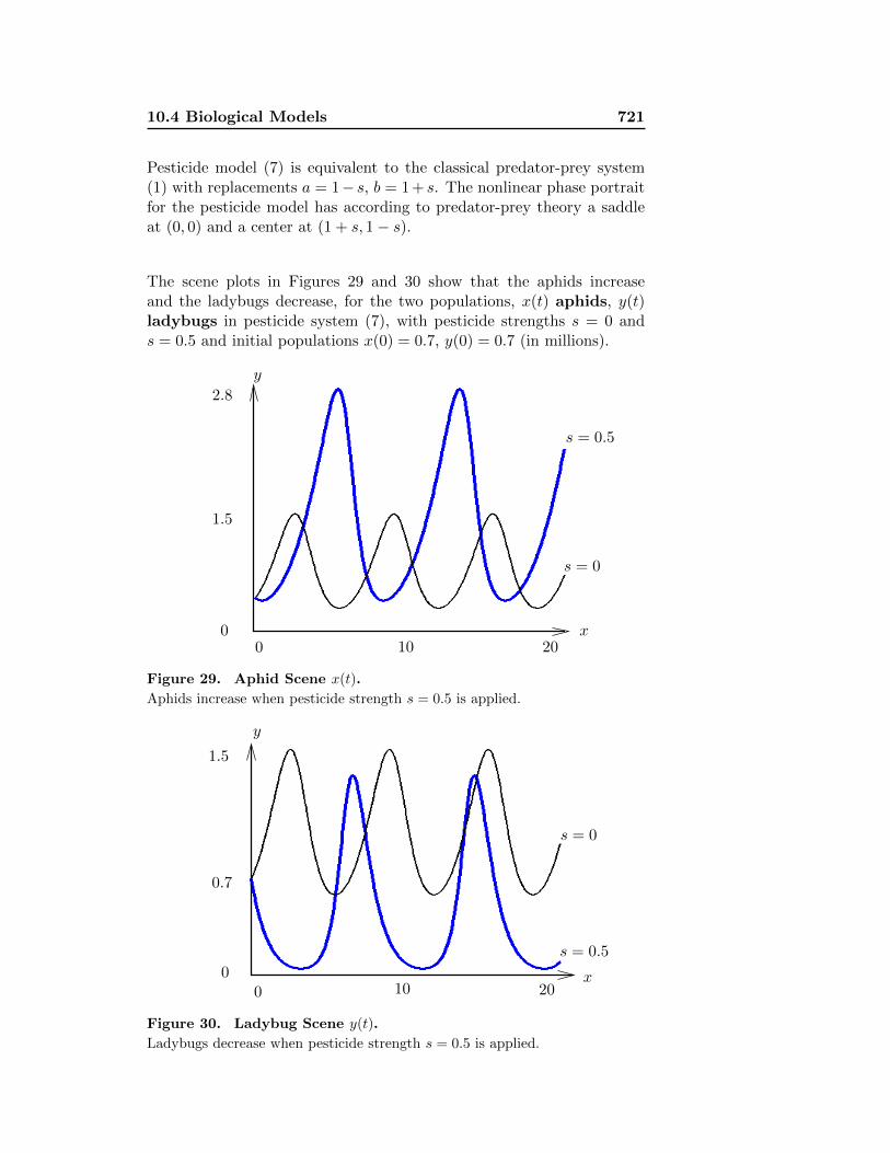
Pesticide model (7) is equivalent to the classical predator-prey system(1) with replacements a = 1− s, b = 1 + s. The nonlinear phase portraitfor the pesticide model has according to predator-prey theory a saddleat (0, 0) and a center at (1 + s, 1− s).
The scene plots in Figures 29 and 30 show that the aphids increaseand the ladybugs decrease, for the two populations, x(t) aphids, y(t)ladybugs in pesticide system (7), with pesticide strengths s = 0 ands = 0.5 and initial populations x(0) = 0.7, y(0) = 0.7 (in millions).
y
10 20x0
1.5
2.8
s = 0
s = 0.5
0
Figure 29. Aphid Scene x(t).
Aphids increase when pesticide strength s = 0.5 is applied.
y
0.7
1.5
x
s = 0
s = 0.5
00 10 20
Figure 30. Ladybug Scene y(t).
Ladybugs decrease when pesticide strength s = 0.5 is applied.
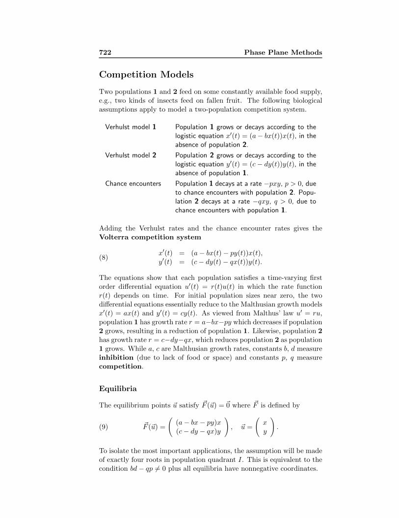
722 Phase Plane Methods
Competition Models
Two populations 1 and 2 feed on some constantly available food supply,e.g., two kinds of insects feed on fallen fruit. The following biologicalassumptions apply to model a two-population competition system.
Verhulst model 1 Population 1 grows or decays according to thelogistic equation x′(t) = (a− bx(t))x(t), in theabsence of population 2.
Verhulst model 2 Population 2 grows or decays according to thelogistic equation y′(t) = (c− dy(t))y(t), in theabsence of population 1.
Chance encounters Population 1 decays at a rate −pxy, p > 0, dueto chance encounters with population 2. Popu-lation 2 decays at a rate −qxy, q > 0, due tochance encounters with population 1.
Adding the Verhulst rates and the chance encounter rates gives theVolterra competition system
x′(t) = (a− bx(t)− py(t))x(t),y′(t) = (c− dy(t)− qx(t))y(t).
(8)
The equations show that each population satisfies a time-varying firstorder differential equation u′(t) = r(t)u(t) in which the rate functionr(t) depends on time. For initial population sizes near zero, the twodifferential equations essentially reduce to the Malthusian growth modelsx′(t) = ax(t) and y′(t) = cy(t). As viewed from Malthus’ law u′ = ru,population 1 has growth rate r = a−bx−py which decreases if population2 grows, resulting in a reduction of population 1. Likewise, population 2has growth rate r = c−dy−qx, which reduces population 2 as population1 grows. While a, c are Malthusian growth rates, constants b, d measureinhibition (due to lack of food or space) and constants p, q measurecompetition.
Equilibria
The equilibrium points ~u satisfy ~F (~u) = ~0 where ~F is defined by
~F (~u) =
((a− bx− py)x(c− dy − qx)y
), ~u =
(xy
).(9)
To isolate the most important applications, the assumption will be madeof exactly four roots in population quadrant I. This is equivalent to thecondition bd− qp 6= 0 plus all equilibria have nonnegative coordinates.
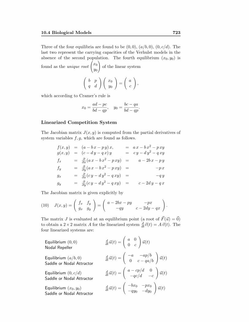
10.4 Biological Models 723
Three of the four equilibria are found to be (0, 0), (a/b, 0), (0, c/d). Thelast two represent the carrying capacities of the Verhulst models in theabsence of the second population. The fourth equilibrium (x0, y0) is
found as the unique root
(x0y0
)of the linear system
(b pq d
)(x0y0
)=
(ac
),
which according to Cramer’s rule is
x0 =ad− pcbd− qp
, y0 =bc− qabd− qp
.
Linearized Competition System
The Jacobian matrix J(x, y) is computed from the partial derivatives ofsystem variables f, g, which are found as follows.
f(x, y) = (a− b x− p y)x, = a x− b x2 − p xyg(x, y) = (c− d y − q x) y = c y − d y2 − q xyfx = ∂
∂x(a x− b x2 − p xy) = a− 2b x− p yfy = ∂
∂y (a x− b x2 − p xy) = −p xgx = ∂
∂x(c y − d y2 − q xy) = −q ygy = ∂
∂y (c y − d y2 − q xy) = c− 2d y − q x
The Jacobian matrix is given explicitly by
J(x, y) =
(fx fygx gy
)=
(a− 2bx− py −px−qy c− 2dy − qx
).(10)
The matrix J is evaluated at an equilibrium point (a root of ~F (~u) = ~0)to obtain a 2×2 matrix A for the linearized system d
dt~v(t) = A~v(t). Thefour linearized systems are:
Equilibrium (0, 0)Nodal Repeller
ddt~u(t) =
(a 00 c
)~u(t)
Equilibrium (a/b, 0)Saddle or Nodal Attractor
ddt~u(t) =
(−a −ap/b0 c− qa/b
)~u(t)
Equilibrium (0, c/d)Saddle or Nodal Attractor
ddt~u(t) =
(a− cp/d 0−qc/d −c
)~u(t)
Equilibrium (x0, y0)Saddle or Nodal Attractor
ddt~u(t) =
(−bx0 −px0−qy0 −dy0
)~u(t)
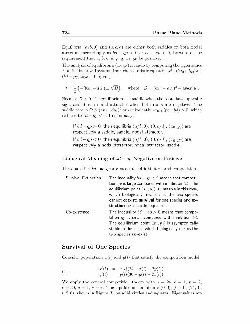
724 Phase Plane Methods
Equilibria (a/b, 0) and (0, c/d) are either both saddles or both nodalatractors, accordingly as bd − qp > 0 or bd − qp < 0, because of therequirement that a, b, c, d, p, q, x0, y0 be positive.
The analysis of equilibrium (x0, y0) is made by computing the eigenvaluesλ of the linearized system, from characteristic equation λ2+(bx0+dy0)λ+(bd− pq)x0y0 = 0, giving
λ =1
2
(−(bx0 + dy0)±
√D), where D = (bx0 − dy0)2 + 4pqx0y0.
Because D > 0, the equilibrium is a saddle when the roots have oppositesign, and it is a nodal attractor when both roots are negative. Thesaddle case is D > (bx0 +dy0)
2 or equivalently 4x0y0(pq−bd) > 0, whichreduces to bd− qp < 0. In summary:
If bd− qp > 0, then equilibria (a/b, 0), (0, c/d), (x0, y0) arerespectively a saddle, saddle, nodal attractor.
If bd− qp < 0, then equilibria (a/b, 0), (0, c/d), (x0, y0) arerespectively a nodal attractor, nodal attractor, saddle.
Biological Meaning of bd− qp Negative or Positive
The quantities bd and qp are measures of inhibition and competition.
Survival-Extinction The inequality bd− qp < 0 means that competi-tion qp is large compared with inhibition bd. Theequilibrium point (x0, y0) is unstable in this case,which biologically means that the two speciescannot coexist: survival for one species and ex-tinction for the other species.
Co-existence The inequality bd − qp > 0 means that compe-tition qp is small compared with inhibition bd.The equilibrium point (x0, y0) is asymptoticallystable in this case, which biologically means thetwo species co-exist.
Survival of One Species
Consider populations x(t) and y(t) that satisfy the competition model
x′(t) = x(t)(24− x(t)− 2y(t)),y′(t) = y(t)(30− y(t)− 2x(t)).
(11)
We apply the general competition theory with a = 24, b = 1, p = 2,c = 30, d = 1, q = 2. The equilibrium points are (0, 0), (0, 30), (24, 0),(12, 6), shown in Figure 31 as solid circles and squares. Eigenvalues are
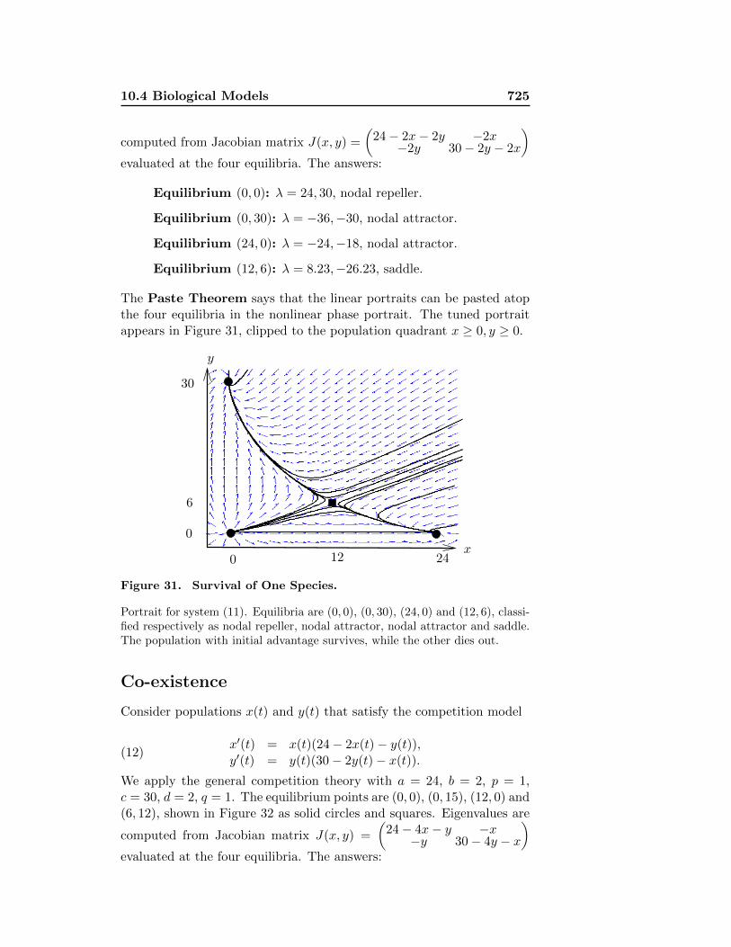
10.4 Biological Models 725
computed from Jacobian matrix J(x, y) =
(24− 2x− 2y −2x−2y 30− 2y − 2x
)evaluated at the four equilibria. The answers:
Equilibrium (0, 0): λ = 24, 30, nodal repeller.
Equilibrium (0, 30): λ = −36,−30, nodal attractor.
Equilibrium (24, 0): λ = −24,−18, nodal attractor.
Equilibrium (12, 6): λ = 8.23,−26.23, saddle.
The Paste Theorem says that the linear portraits can be pasted atopthe four equilibria in the nonlinear phase portrait. The tuned portraitappears in Figure 31, clipped to the population quadrant x ≥ 0, y ≥ 0.
0
30
24120
6
y
x
Figure 31. Survival of One Species.
Portrait for system (11). Equilibria are (0, 0), (0, 30), (24, 0) and (12, 6), classi-fied respectively as nodal repeller, nodal attractor, nodal attractor and saddle.The population with initial advantage survives, while the other dies out.
Co-existence
Consider populations x(t) and y(t) that satisfy the competition model
x′(t) = x(t)(24− 2x(t)− y(t)),y′(t) = y(t)(30− 2y(t)− x(t)).
(12)
We apply the general competition theory with a = 24, b = 2, p = 1,c = 30, d = 2, q = 1. The equilibrium points are (0, 0), (0, 15), (12, 0) and(6, 12), shown in Figure 32 as solid circles and squares. Eigenvalues are
computed from Jacobian matrix J(x, y) =
(24− 4x− y −x−y 30− 4y − x
)evaluated at the four equilibria. The answers:
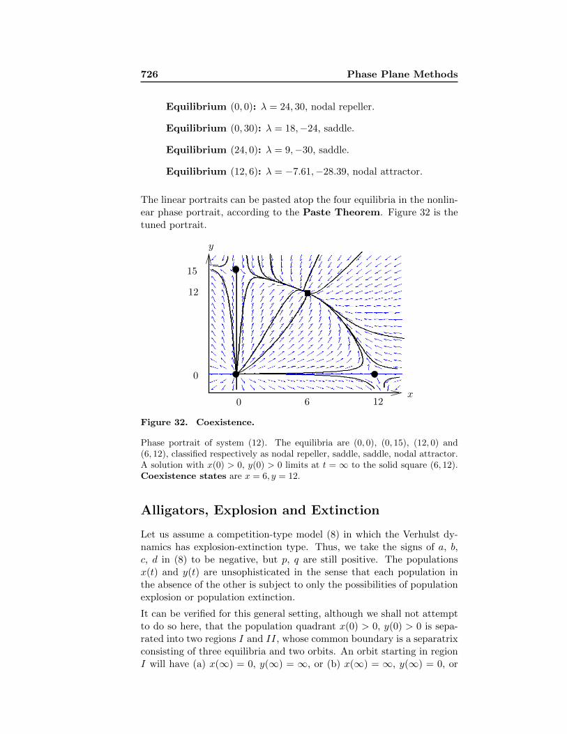
726 Phase Plane Methods
Equilibrium (0, 0): λ = 24, 30, nodal repeller.
Equilibrium (0, 30): λ = 18,−24, saddle.
Equilibrium (24, 0): λ = 9,−30, saddle.
Equilibrium (12, 6): λ = −7.61,−28.39, nodal attractor.
The linear portraits can be pasted atop the four equilibria in the nonlin-ear phase portrait, according to the Paste Theorem. Figure 32 is thetuned portrait.
y
x60 12
0
12
15
Figure 32. Coexistence.
Phase portrait of system (12). The equilibria are (0, 0), (0, 15), (12, 0) and(6, 12), classified respectively as nodal repeller, saddle, saddle, nodal attractor.A solution with x(0) > 0, y(0) > 0 limits at t = ∞ to the solid square (6, 12).Coexistence states are x = 6, y = 12.
Alligators, Explosion and Extinction
Let us assume a competition-type model (8) in which the Verhulst dy-namics has explosion-extinction type. Thus, we take the signs of a, b,c, d in (8) to be negative, but p, q are still positive. The populationsx(t) and y(t) are unsophisticated in the sense that each population inthe absence of the other is subject to only the possibilities of populationexplosion or population extinction.
It can be verified for this general setting, although we shall not attemptto do so here, that the population quadrant x(0) > 0, y(0) > 0 is sepa-rated into two regions I and II, whose common boundary is a separatrixconsisting of three equilibria and two orbits. An orbit starting in regionI will have (a) x(∞) = 0, y(∞) = ∞, or (b) x(∞) = ∞, y(∞) = 0, or
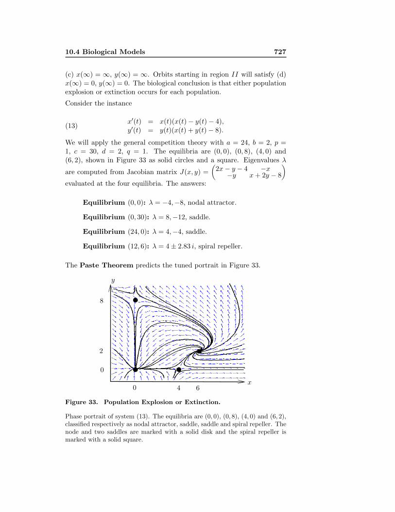
10.4 Biological Models 727
(c) x(∞) = ∞, y(∞) = ∞. Orbits starting in region II will satisfy (d)x(∞) = 0, y(∞) = 0. The biological conclusion is that either populationexplosion or extinction occurs for each population.
Consider the instance
x′(t) = x(t)(x(t)− y(t)− 4),y′(t) = y(t)(x(t) + y(t)− 8).
(13)
We will apply the general competition theory with a = 24, b = 2, p =1, c = 30, d = 2, q = 1. The equilibria are (0, 0), (0, 8), (4, 0) and(6, 2), shown in Figure 33 as solid circles and a square. Eigenvalues λ
are computed from Jacobian matrix J(x, y) =
(2x− y − 4 −x−y x+ 2y − 8
)evaluated at the four equilibria. The answers:
Equilibrium (0, 0): λ = −4,−8, nodal attractor.
Equilibrium (0, 30): λ = 8,−12, saddle.
Equilibrium (24, 0): λ = 4,−4, saddle.
Equilibrium (12, 6): λ = 4± 2.83 i, spiral repeller.
The Paste Theorem predicts the tuned portrait in Figure 33.
0 4 6
2
0
8
y
x
Figure 33. Population Explosion or Extinction.
Phase portrait of system (13). The equilibria are (0, 0), (0, 8), (4, 0) and (6, 2),classified respectively as nodal attractor, saddle, saddle and spiral repeller. Thenode and two saddles are marked with a solid disk and the spiral repeller ismarked with a solid square.
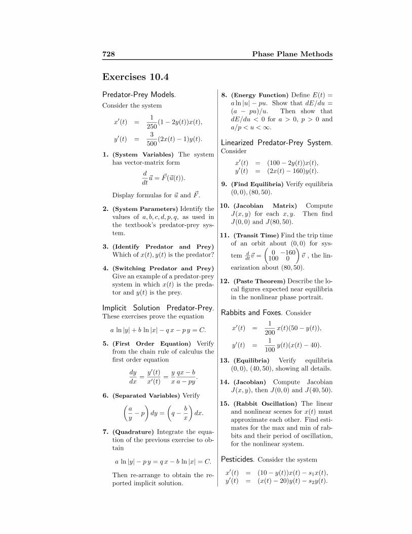
728 Phase Plane Methods
Exercises 10.4
Predator-Prey Models.
Consider the system
x′(t) =1
250(1− 2y(t))x(t),
y′(t) =3
500(2x(t)− 1)y(t).
1. (System Variables) The systemhas vector-matrix form
d
dt~u = ~F (~u(t)).
Display formulas for ~u and ~F .
2. (System Parameters) Identify thevalues of a, b, c, d, p, q, as used inthe textbook’s predator-prey sys-tem.
3. (Identify Predator and Prey)
Which of x(t), y(t) is the predator?
4. (Switching Predator and Prey)
Give an example of a predator-preysystem in which x(t) is the preda-tor and y(t) is the prey.
Implicit Solution Predator-Prey.These exercises prove the equation
a ln |y|+ b ln |x| − q x− p y = C.
5. (First Order Equation) Verifyfrom the chain rule of calculus thefirst order equation
dy
dx=y′(t)
x′(t)=y
x
qx− ba− py
.
6. (Separated Variables) Verify(a
y− p)dy =
(q − b
x
)dx.
7. (Quadrature) Integrate the equa-tion of the previous exercise to ob-tain
a ln |y| − p y = q x− b ln |x| = C.
Then re-arrange to obtain the re-ported implicit solution.
8. (Energy Function) Define E(t) =a ln |u| − pu. Show that dE/du =(a − pu)/u. Then show thatdE/du < 0 for a > 0, p > 0 anda/p < u <∞.
Linearized Predator-Prey System.Consider
x′(t) = (100− 2y(t))x(t),y′(t) = (2x(t)− 160)y(t).
9. (Find Equilibria) Verify equilibria(0, 0), (80, 50).
10. (Jacobian Matrix) ComputeJ(x, y) for each x, y. Then findJ(0, 0) and J(80, 50).
11. (Transit Time) Find the trip timeof an orbit about (0, 0) for sys-
tem ddt~v =
(0 −160
100 0
)~v , the lin-
earization about (80, 50).
12. (Paste Theorem) Describe the lo-cal figures expected near equilibriain the nonlinear phase portrait.
Rabbits and Foxes. Consider
x′(t) =1
200x(t)(50− y(t)),
y′(t) =1
100y(t)(x(t)− 40).
13. (Equilibria) Verify equilibria(0, 0), (40, 50), showing all details.
14. (Jacobian) Compute JacobianJ(x, y), then J(0, 0) and J(40, 50).
15. (Rabbit Oscillation) The linearand nonlinear scenes for x(t) mustapproximate each other. Find esti-mates for the max and min of rab-bits and their period of oscillation,for the nonlinear system.
Pesticides. Consider the system
x′(t) = (10− y(t))x(t)− s1x(t),y′(t) = (x(t)− 20)y(t)− s2y(t).
10.4 Biological Models 729
16. (Equilibria) Show details for com-puting the pesticide system equilib-ria (0, 0), (20 + s2, 10 − s1), wheres1, s2 are the pesticide death rates.
17. (Average Populations) Explain:A field biologist should count, onthe average, populations of about20 + s2 prey and 10− s1 predators.
Survival of One Species. Consider
x′(t) = x(t)(24− x(t)− 2y(t)),y′(t) = y(t)(30− y(t)− 2x(t)).
18. (Interactions) Show that dou-bling either x or y causes the in-teraction term 2xy to double.
19. (Equilibria) Find all equilibria.
20. (Linearization) Find the lin-earized systems d
dt~v = J(x0, y0)~vfor each equilibrium point (x0, y0).
21. (Nonlinear Classification) Clas-sify each equilibrium point (x0, y0)as center, spiral, node, saddle, us-ing the Paste Theorem. Make aphase portrait which confirms theclassifications.
Co-existence.
Explosion and Extinction.
730 Phase Plane Methods
10.5 Mechanical Models
Nonlinear Spring-Mass System
The classical linear undamped spring-mass system is modeled by theequation mx′′(t) + kx(t) = 0. This equation describes the excursion x(t)from equilibrium x = 0 of a mass m attached to a spring of Hooke’sconstant k, with no damping and no external forces.
In the nonlinear theory, the Hooke’s force term −kx is replaced by arestoring force F (x) which satisfies these four requirements:
Equilibrium 0. The equation F (0) = 0 is assumed, which gives x = 0the status of a rest position.
Oddness. The equation F (−x) = −F (x) is assumed, which says thatthe force F depends only upon the magnitude of the excursionfrom equilibrium, and not upon its direction. Then force F acts torestore the mass to its equilibrium position, like a Hooke’s forcex→ kx.
Zero damping. The damping effects always present in a real physicalsystem are ignored. In linear approximations, it would be usual toassume a viscous damping effect −cx′(t); from this viewpoint weassume c = 0.
Zero external force. There is no external force acting on the system.In short, only two forces act on the mass, (1) Newton’s second lawand (2) restoring force F .
The competition method applies to model the nonlinear spring-mass sys-tem via the two competing forces mx′′(t) and F (x(t)). The dynamicalequation:
mx′′(t) + F (x(t)) = 0.(1)
Soft and Hard Springs
A restoring force F modeled upon Hooke’s law is given by the equationF (x) = kx. With this force, the nonlinear spring-mass equation (1)becomes the undamped linear spring-mass system
mx′′(t) + kx(t) = 0.(2)
The linear equation can be thought to originate by replacing the actualspring force F by the first nonzero term of its Taylor series
F (x) = F (0) + F ′(0)x+ F ′′(0)x2
2!+ · · · .
10.5 Mechanical Models 731
The assumptions F (−x) = −F (x) and F (0) = 0 imply that F (x) is afunction of the form F (x) = xG(x2), hence all even terms in the Taylorseries of F are zero.
Linear approximations to the force F drop the quadratic terms andhigher from the Taylor series. More accurate nonlinear approximationsare obtained by retaining extra Taylor series terms.
A restoring force F is called hard or soft provided it is given by atruncated Taylor series as follows.
Hard spring F (x) = kx+ βx3, β > 0.
Soft spring F (x) = kx− βx3, β > 0.
For small excursions from equilibrium x = 0, a hard or soft springforce has magnitude approximately the same as the linear Hooke’s forceF (x) = kx.
Energy Conservation. Each solution x(t) of the nonlinear spring-mass equation mx′′(t) + F (x(t)) = 0 satisfies on its domain of existencethe conservation law
m
2(x′(t))2 +
∫ x(t)
x(0)F (u) du = C, C ≡ m
2(x′(0))2.(3)
To prove the law, multiply the nonlinear differential equation by x′(t) toobtain mx′′(t)x′(t) + F (x(t))x′(t) = 0, then apply quadrature to obtain(3).
Kinetic and Potential Energy. Using v = x′(t), the term mv2/2in (3) is called the kinetic energy (KE) and the term
∫ xx0F (u)du is
called the potential energy (PE). Equation (3) says that KE+PE =C or that energy is constant along trajectories.
The conservation laws for the soft and hard nonlinear spring-mass sys-tems, using position-velocity notation x = x(t) and y = x′(t), are there-fore given by the equations
my2 + kx2 +1
2βx4 = C1, C1 = constant > 0,(4)
my2 + kx2 − 1
2βx4 = C2, C2 = constant.(5)
Phase Plane and Scenes. Nonlinear behavior is commonly graphedin the phase plane, in which x = x(t) and y = x′(t) are the position andvelocity of the mechanical system. The plots of t versus x(t) or x′(t) arecalled scenes; these plots are invaluable for verifying periodic behaviorand stability properties.
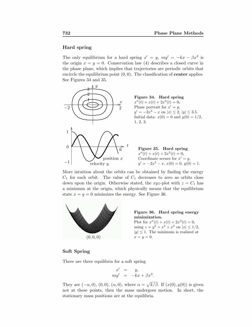
732 Phase Plane Methods
Hard spring
The only equilibrium for a hard spring x′ = y, my′ = −kx − βx3 isthe origin x = y = 0. Conservation law (4) describes a closed curve inthe phase plane, which implies that trajectories are periodic orbits thatencircle the equilibrium point (0, 0). The classification of center applies.See Figures 34 and 35.
y
−2
321
2
xFigure 34. Hard springx′′(t) + x(t) + 2x3(t) = 0.Phase portrait for x′ = y,y′ = −2x3 − x on |x| ≤ 2, |y| ≤ 3.5.Initial data: x(0) = 0 and y(0) = 1/2,1, 2, 3.
−1
1
06
t
velocity yposition x
Figure 35. Hard springx′′(t) + x(t) + 2x3(t) = 0.Coordinate scenes for x′ = y,y′ = −2x3 − x, x(0) = 0, y(0) = 1.
More intuition about the orbits can be obtained by finding the energyC1 for each orbit. The value of C1 decreases to zero as orbits closedown upon the origin. Otherwise stated, the xyz-plot with z = C1 hasa minimum at the origin, which physically means that the equilibriumstate x = y = 0 minimizes the energy. See Figure 36.
(0, 0, 0)
Figure 36. Hard spring energyminimization.Plot for x′′(t) + x(t) + 2x3(t) = 0,using z = y2 + x2 + x4 on |x| ≤ 1/2,|y| ≤ 1. The minimum is realized atx = y = 0.
Soft Spring
There are three equilibria for a soft spring
x′ = y,my′ = −kx+ βx3.
They are (−α, 0), (0, 0), (α, 0), where α =√k/β. If (x(0), y(0)) is given
not at these points, then the mass undergoes motion. In short, thestationary mass positions are at the equilibria.
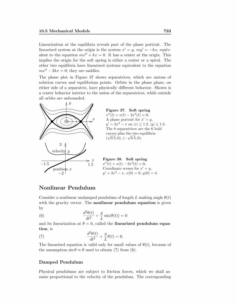
10.5 Mechanical Models 733
Linearization at the equilibria reveals part of the phase portrait. Thelinearized system at the origin is the system x′ = y, my′ = −kx, equiv-alent to the equation mx′′ + kx = 0. It has a center at the origin. Thisimplies the origin for the soft spring is either a center or a spiral. Theother two equilibria have linearized systems equivalent to the equationmx′′ − 2kx = 0; they are saddles.
The phase plot in Figure 37 shows separatrices, which are unions ofsolution curves and equilibrium points. Orbits in the phase plane, oneither side of a separatrix, have physically different behavior. Shown isa center behavior interior to the union of the separatrices, while outsideall orbits are unbounded.
y
x
Figure 37. Soft springx′′(t) + x(t)− 2x3(t) = 0.A phase portrait for x′ = y,y′ = 2x3 − x on |x| ≤ 1.2, |y| ≤ 1.2.The 8 separatrices are the 6 boldcurves plus the two equilibria(√
0.5, 0), (−√
0.5, 0).
−2
−1.5 1.5position x
velocity y
t
3
Figure 38. Soft springx′′(t) + x(t)− 2x3(t) = 0.Coordinate scenes for x′ = y,y′ = 2x3 − x, x(0) = 0, y(0) = 4.
Nonlinear Pendulum
Consider a nonlinear undamped pendulum of length L making angle θ(t)with the gravity vector. The nonlinear pendulum equation is givenby
d2θ(t)
dt2+g
Lsin(θ(t)) = 0(6)
and its linearization at θ = 0, called the linearized pendulum equa-tion, is
d2θ(t)
dt2+g
Lθ(t) = 0.(7)
The linearized equation is valid only for small values of θ(t), because ofthe assumption sin θ ≈ θ used to obtain (7) from (6).
Damped Pendulum
Physical pendulums are subject to friction forces, which we shall as-sume proportional to the velocity of the pendulum. The corresponding
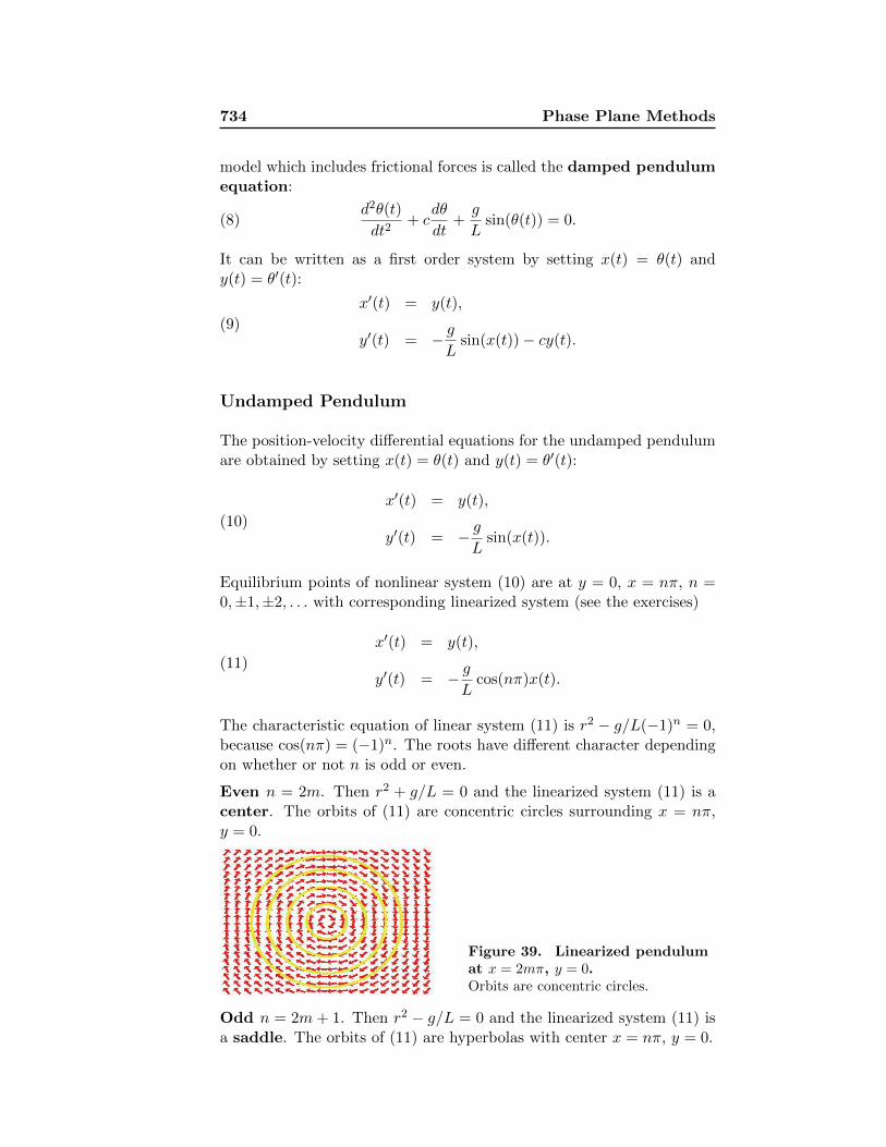
734 Phase Plane Methods
model which includes frictional forces is called the damped pendulumequation:
d2θ(t)
dt2+ c
dθ
dt+g
Lsin(θ(t)) = 0.(8)
It can be written as a first order system by setting x(t) = θ(t) andy(t) = θ′(t):
x′(t) = y(t),
y′(t) = − gL
sin(x(t))− cy(t).(9)
Undamped Pendulum
The position-velocity differential equations for the undamped pendulumare obtained by setting x(t) = θ(t) and y(t) = θ′(t):
x′(t) = y(t),
y′(t) = − gL
sin(x(t)).(10)
Equilibrium points of nonlinear system (10) are at y = 0, x = nπ, n =0,±1,±2, . . . with corresponding linearized system (see the exercises)
x′(t) = y(t),
y′(t) = − gL
cos(nπ)x(t).(11)
The characteristic equation of linear system (11) is r2 − g/L(−1)n = 0,because cos(nπ) = (−1)n. The roots have different character dependingon whether or not n is odd or even.
Even n = 2m. Then r2 + g/L = 0 and the linearized system (11) is acenter. The orbits of (11) are concentric circles surrounding x = nπ,y = 0.
Figure 39. Linearized pendulumat x = 2mπ, y = 0.Orbits are concentric circles.
Odd n = 2m+ 1. Then r2 − g/L = 0 and the linearized system (11) isa saddle. The orbits of (11) are hyperbolas with center x = nπ, y = 0.
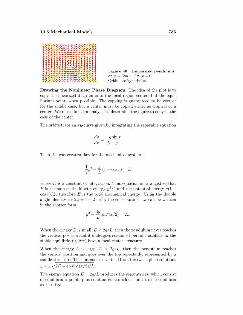
10.5 Mechanical Models 735
Figure 40. Linearized pendulumat x = (2m+ 1)π, y = 0.Orbits are hyperbolas.
Drawing the Nonlinear Phase Diagram. The idea of the plot is tocopy the linearized diagram onto the local region centered at the equi-librium point, when possible. The copying is guaranteed to be correctfor the saddle case, but a center must be copied either as a spiral or acenter. We must do extra analysis to determine the figure to copy in thecase of the center.
The orbits trace an xy-curve given by integrating the separable equation
dy
dx=−gL
sinx
y.
Then the conservation law for the mechanical system is
1
2y2 +
g
L(1− cosx) = E
where E is a constant of integration. This equation is arranged so thatE is the sum of the kinetic energy y2/2 and the potential energy g(1 −cosx)/L, therefore E is the total mechanical energy. Using the doubleangle identity cos 2φ = 1 − 2 sin2 φ the conservation law can be writtenin the shorter form
y2 +4g
Lsin2(x/2) = 2E
When the energy E is small, E < 2g/L, then the pendulum never reachesthe vertical position and it undergoes sustained periodic oscillation: thestable equilibria (0, 2kπ) have a local center structure.
When the energy E is large, E > 2g/L, then the pendulum reachesthe vertical position and goes over the top repeatedly, represented by asaddle structure. The statement is verified from the two explicit solutions
y = ±√
2E − 4g sin2(x/2)/L.
The energy equation E = 2g/L produces the separatrices, which consistof equilibrium points plus solution curves which limit to the equilibriaas t→ ±∞.
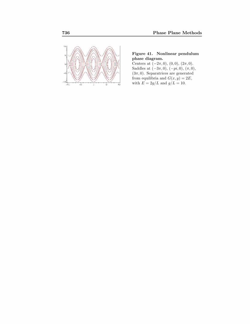
736 Phase Plane Methods
Figure 41. Nonlinear pendulumphase diagram.Centers at (−2π, 0), (0, 0), (2π, 0).Saddles at (−3π, 0), (−pi, 0), (π, 0),(3π, 0). Separatrices are generatedfrom equilibria and G(x, y) = 2E,with E = 2g/L and g/L = 10.