Phase diagram of a Schelling segregation model

L. Gauvin ∗1, J. Vannimenus1, and J.-P. Nadal1,2

1Laboratoire de Physique Statistique (UMR 8550 CNRS-ENS-Paris 6-Paris 7),Ecole Normale Superieure, Paris, France

2Centre d’Analyse et de Mathematique Sociales (UMR 8557 CNRS-EHESS), Ecoledes Hautes Etudes en Sciences Sociales, Paris, France

26 March 2009

Abstract

The collective behavior in a variant of Schelling’s segregation model is characterized withmethods borrowed from statistical physics, in a context where their relevance was not conspic-uous. A measure of segregation based on cluster geometry is defined and several quantitiesanalogous to those used to describe physical lattice models at equilibrium are introduced. Thisphysical approach allows to distinguish quantitatively several regimes and to characterize thetransitions between them, leading to the building of a phase diagram. Some of the transitionsevoke empirical sudden ethnic turnovers. We also establish links with ’spin-1’ models in physics.Our approach provides generic tools to analyze the dynamics of other socio-economic systems.

Keywords: segregation – Schelling model – phase diagram – discontinuous transition –Blume-Capel model – Blume-Emery-Griffiths model

Introduction

In the course of his study of the segregation effects observed in many social situations, ThomasSchelling introduced in the 1970’s [1, 2] a model that has attracted a lot of attention ever since,to the point that it may now be considered an archetype in the social sciences. The success ofthe Schelling model is due to several factors: It was one of the first models of a complex systemto show emergent behavior due to interactions among agents; it is very simple to describe, yet itsmain outcome - that strong segregation effects can arise from rather weak individual preferences- came as a surprise and proved robust with respect to various more realistic refinements; as aconsequence, it has possibly far-reaching implications for social and economic policies aiming atfighting urban segregation, considered a major issue in many countries (for recent discussions of thesocial relevance of the model, see [3] and [4]).

An important recent development is the realization that there exists a striking kinship betweenthis model and various physical models used to describe surface tension phenomena [5] or phasetransitions and clustering effects, such as the Ising model [6, 7, 8]. This connection is not a rigorouscorrespondence, still it is more than a mere analogy. It gives novel insight into the behavior ofthe Schelling model, and it suggests more generally that socio-economic models may be fruitfullyattacked drawing from the toolbox of statistical physics [7, 9]. Indeed, physicists developed duringthe last decades powerful methods for situations where obtaining analytical results seems out ofreach. These rely on the quantitative analysis of computer simulation results, guided by somegeneral principles. They are well suited to complex systems such as those encountered in the social

∗Corresponding author, laetitia.gauvin@lps.ens.fr

1

arX

iv:0

903.

4694

v1 [

phys

ics.

soc-

ph]

27

Mar

200

9

sciences and should in particular prove powerful in conjunction with agent-based modeling1, agrowingly popular approach [10].

A key physicist strategy is to characterize the system under study by the phase diagram whichgives, in the space of control parameters, the boundaries separating domains of different qualitativebehaviors. Each type of behavior is qualified by the order of magnitude of a small set of macroscopicquantities, the so-called “order parameters”. The main difficulties are to correctly identify therelevant set of order parameters and the associated qualitative behaviors of the system, and to locateand characterize the boundaries, on which “phase transitions” occur in a smooth or discontinuousway. In the present paper, we show how several of the methods evoked above can be adapted andapplied to the building of the phase diagram of social dynamics models, taking as paradigm theSchelling segregation model. More precisely, we illustrate our approach on a particular variant ofthe Schelling model, where the basic variables are the tolerance (to be defined precisely below)and the density of vacant sites. We introduce two order parameters which provide a relevantmeasure of global segregation, a surrogate of the energy, and analogues of the susceptibility andthe specific heat. We also introduce a real-space renormalization method suited to situations witha high density of vacancies. Our analysis shows the existence in the phase diagram of the modelof sharp transitions, where relevant quantities have singularities, and we discuss the nature ofthese transitions. They separate different types of behavior - segregated, mixed, or ”frozen” -, inagreement with qualitative observations based on pictures of simulated systems [5]. In addition wemake contact with the Blume-Emery-Griffiths [11] and Blume-Capel [12, 13] models, which are spin-1 models much studied in relation with binary mixtures containing mobile vacancies and which showa richer behavior than the simple Ising model, with both discontinuous and continuous transitions.One should insist that most variants of the Schelling segregation model are of kinetic nature: theirdynamics cannot be described as the relaxation to an equilibrium characterized by some energyfunction, except for specific variants (for such exceptions, see e.g. [14, 21] and the discussion belowon the links with spin models). Nevertherless, the tools and quantities we introduce by analogy withequilibrium statistical mechanics appear to be quite efficient to characterize the model behaviors.They are sufficiently general and relatively simple to be adaptable to a large variety of social andeconomic models, as long as these involve interacting agents living in a discrete space or moregenerally on a social network.

1 Model and qualitative analysis

In Schelling’s original model [1] agents of two possible colors are located on the sites of a chessboard.Each color corresponds to members of one of two homogeneous groups which differ for example bytheir race, their wealth, etc... A fraction of the sites are blanks, the agents of both colors may moveto these vacancies. The neighborhood of an agent comprises the eight nearest and next-nearest sites(Moore neighborhood). If less than 1

3 of an agent’s neighbors belong to his group, he is discontent– in economic terms his utility is 0; otherwise he is satisfied - his utility is 1. Starting from randominitial configurations Schelling displaced discontent agents onto the closest satisfactory vacant sites,if possible. He observed that the system always reached a segregated state, where large clustersof same-color agents were formed. The crucial point is that segregation appears as an emergentphenomenon, in the sense that the collective effect is much stronger than what would be naivelyexpected, as individual agents are happy to live in a mixed neighborhood. This phenomenon provesrobust: a similar outcome, with some caveats, is found in variants of the model, even when theutility function is non-monotonous with the fraction of similar neighbors [3, 15].The model we consider is a variant of the original Schelling model: The agents are satisfied withtheir neighborhood if it is constituted of a number of unlike agents Nd lower than (or equal to) afixed proportion T of all the agents in the neighborhood. The parameter T is called the tolerance[1]. Since a higher tolerance allows for a larger number of configurations of satisfied agents (higherentropy), this parameter may be thought of as a temperature-like variable. We will be guided bythis qualitative correspondence – although in a different way than in [6], where a direct analogy is

1The ’hand-made simulations’ done by T. Schelling by moving pawns on a chessboard can be considered as thefirst agent-based simulations ever done in social science.

2

made with the Ising model. The other control parameter of the model is the vacancy density ρ. Therandomly chosen agents move one by one to any vacancy which has a satisfying neighborhood - thisis equivalent to long-range diffusion in physical terms. If no vacancy fits for some agents the latterrespectively move back to their initial position. This dynamics is repeated until configurations arereached where the number of satisfied agents is almost stable. Note that in the present variantsatisfied agents can also move, not just discontent ones. That rule introduces some noise in thedynamics and is useful to avoid a particularity of the original Schelling model noted in [6, 14],namely that the system may end up in states where the clusters are large but finite, so that strictlyspeaking no large-scale segregation occurs. We will see later how the intensity of this noise is actuallycorrelated with the tolerance level T . Note also that the global utility may decrease at times duringthe process, as the gain for the moved agent can be less than the net loss for his old plus newneighbors [2]. Let us emphasize that only a finite number of values of T are meaningful, namely18 ,

17 ...,

67 ,

78 . They correspond to the maximal number of tolerated different neighbors divided by

the actual number of occupied sites in the neighborhood. Any other value for T is thus equivalentto the closest inferior meaningful value.

1.1 Numerical Simulations.

Our simulations were performed on a L × L lattice (L = 50, unless otherwise specified) with freeboundary conditions. An initial configuration was randomly generated such that the vacancies andthe two types of agents were fully mixed. Then the evolution followed the rules described above.In the simulations one time step corresponds to one attempted move per occupied site on average,the usual definition of a Monte-Carlo step.

Figure 1: Evolution of the configuration for a vacancy concentration ρ = 5% and a tolerance T = 0.5with a network size L = 100. St stands for the number of time steps. The red and blue pixelscorrespond to the two types of agents, the white pixels to the vacancies. The system evolves froma random configuration – where the vacancies and the two types of agents are intimately mixed –to a completely segregated configuration. After just 10 steps there exist two percolating clusters,one of each color, which are very convoluted, fractal-like.

Fig. 1 shows the time evolution of a typical configuration, for a vacancy density of 5% and atolerance T = 0.5, which means that agents accept at most half of their neighbors to be differentfrom themselves. One observes the rapid formation of large clusters. After 10 time steps, theproportion of satisfied agents is already very close to 1 (Appendix, Fig. A.2). It increases slowlythereafter, but the structure of the clusters keeps evolving. They become more and more compactand well separated spatially, their surface gets less corrugated, in a process strongly reminiscentof coarsening effects in alloys [16]. We now consider more general values of the tolerance and thevacancy density. Fig. 2 shows configurations obtained after letting the system evolve with thedynamics previously described until it reaches equilibrium. What is meant by equilibrium here maycorrespond to two different situations: (i) The system does not evolve at all anymore (fixed point);(ii) The systems reaches some stationary state: the fluctuations of the studied parameters remainweak during a large number of time steps. In the following all averaged quantities are measuredduring 30000 steps after equilibrium is reached.

At small and moderate values of ρ, one observes that :– For low values of the tolerance the system stays in a mixed state, no large one-color clusters

are formed although this would be more satisfactory for the agents. Actually, whatever the initialconfiguration, the system remains close to the state in which it was created: this is a dynamicallyfrozen state.

3

Figure 2: Configurations obtained at large times for selected values of ρ and T .

– When T increases, at fixed ρ, a drastic qualitative change occurs at an intermediate value ofT : The system separates into two homogeneous regions of different colors, segregation occurs. Thisbehavior subsists for an interval of T which depends on ρ.

– For T larger than a value weakly depending on ρ, the final configuration is again mixed.For large values of ρ one observes a smooth transition as T increases from a segregated state toa mixed one. We will now give a more quantitative description and characterize the transitionsbetween these different behaviors.

2 Quantitative analysis: order parameters

2.1 Main order parameter: A measure of segregation

Though the presence of segregation in a system can be visually assessed, a quantitative way tomeasure it is necessary, in particular to discuss the nature of the transitions between differentstates. Different possible measures have been suggested, by Schelling himself and later by variousauthors [3, 14, 17], which capture various aspects of the phenomenon. Here we introduce a measurelinked to the definition of segregation as the grouping of agents of the same type and the exclusionof the other type in a given area. To that effect we consider that two agents belong to the samecluster if they are nearest neighbors (the Moore neighborhood cannot be used here, since Mooreclusters of different colors may overlap and be large without segregation occurring). The (mass) sizeof a cluster c, i.e the number of agents it contains, will be called nc. Taking a hint from percolationtheory where it plays a central role [18], we introduce the weighted average S of the size of theclusters in one configuration

S =∑{c}

nc pc (1)

where pc = nc

Ntotis the weight of cluster c, Ntot = L2(1− ρ) being the total number of agents. The

maximal size of a cluster is Ntot/2, so the normalized weighted cluster size s is given by

s =2

L2(1− ρ)S =

2(L2(1− ρ))2

∑{c}

nc2 (2)

The sample average of s after reaching equilibrium will be called the segregation coefficient 〈s〉.Its value for complete segregation (i.e., only two clusters survive) is 1 and it vanishes if the size

4

of the clusters remains finite when the system dimension L tends to infinity. It may thereforeplay the role of an order parameter to identify a segregation transition. The variation of thesegregation coefficient 〈s〉 with respect to the tolerance is illustrated in Fig. 3 for different values ofthe vacancy density. The calculations were done using the Hoshen–Kopelman algorithm to labelizethe clusters [19]. For each density of vacancies there exist two critical values of the tolerance. At

0

0.2

0.4

0.6

0.8

1

0.2 0.4 0.6 0.8

Segr

egat

ion

Coef

ficie

nt

Tolerance T

ρ = 2%

ρ = 6%

ρ = 12%

ρ = 18%

ρ = 26%

Figure 3: Segregation coefficient (average of s defined in Eq. (2)) for several values of the vacancydensity ρ. The lines linking the points are guides to the eye.

the first one Tf (f for frozen), 〈s〉 jumps from a very low value to about 1. This signals an abruptchange from a mixed configuration to one with only two clusters (one for each type of agent). Asecond jump, in the reverse direction, occurs for a larger tolerance Tc. This second value dependsslightly on ρ, unlike Tf . The higher the density of vacancies, the smaller the value of T at whichthe segregation phenomenon appears and the broader the interval of T for which it exists. For avacancy density above about 20% the segregation coefficient departs from 1 (Fig. 3), even if theagents are visually segregated (Fig. 2.1). This is due to the definition of a cluster based only on thefour nearest neighbors. In some regions, even if there are agents of one color only the presence ofmany vacancies may lead to group them into distinct clusters and to miss the existence of a ”dilutesegregation” situation. In order to identify clusters at a larger scale in such cases we introducea real-space renormalization [20] procedure. An example of the renormalization process for a siteand its neighborhood is illustrated on the left of Fig.2.1. A renormalized configuration is shownon the right part of Fig.2.1 (see the appendix for details on the procedure). The renormalization

Figure 4: Example of renormalization. The renormalization is performed on a configuration corre-sponding to T = 1

5 and ρ = 50%.

has a strong effect for high values of the density of vacancies. For ρ = 50% the configurations arevisually segregated for a range of small and medium values of the tolerance but the raw segregationcoefficient is very small (Fig. 5, left), whereas after renormalization it is very close to 1 (Fig. 5,right). We can conclude that, for values of the vacancy density strictly less than 50%, there is adiscontinuous transition from the segregated to the mixed state (as shown on Fig. 3 for ρ up to

5

0

0.02

0.04

0.06

0.08

0.1

0.2 0.4 0.6 0.8

Segr

egat

ion

coeffic

ient

Tolerance T

0

0.2

0.4

0.6

0.8

1

0.2 0.4 0.6 0.8Tolerance T

Figure 5: Segregation coefficient as a function of the tolerance for ρ = 50%: Raw data (left) andresults for the renormalized systems (right). These suggest that a continuous transition takes placenear T = 0.6. The error bars were obtained by computing the variance σs, σ2

s = 〈s〉2 − 〈s2〉 (samefor Fig.3).

26%). At ρ = 50% the transition becomes continuous – as shown on Fig.5 the order parameterhas a smoother variation –, and there is no longer any clear transition for vacancy densities above∼ 56% (not shown). Moreover, the configurations observed at large ρ suggest the existence of adiluted phase of segregation at high vacancy densities: the two types of agents are not mixed butthere are domains with many small clusters of a same color in a sea of vacancies. As for the frozenstate observed at low T for small ρ, it disappears at some medium value of ρ (compare Fig. 3 withFig. 5, right).

2.2 A second order parameter: densities of unwanted locations.

The segregation coefficient defined above does not allow to distinguish between the mixed state atlow tolerance and the one at high tolerance (Fig.3). However, even if the final configuration is amixed configuration for both situations, the nature of the two states is not the same. An additionalparameter is thus necessary to analyze the results. We introduce the density ρr of empty placeswhere the red agents do not want to move (symmetrically ρb for blue agents). The plot of ρr versus

0

0.2

0.4

0.6

0.8

1

0.2 0.4 0.6 0.8

Vaca

ncy

Den

sity

ρr

Tolerance T

ρ = 2%

ρ = 6%

ρ = 12%

ρ = 18%

Figure 6: Density ρr of vacancies where the red agents would be unsatisfied, for several vacancydensities. The results for the blue agents are similar. Indeed, they play symmetrical roles in thepresent model.

6

the tolerance (Fig.6) shows that this quantity undergoes two jumps for each vacancy density ρ.Until the tolerance reaches Tf no empty space is considered attractive by these agents. Between Tf

and Tc half of the vacant sites are satisfactory for one type of agents. For T larger than Tc almostall empty spaces are acceptable. A representative configuration for a situation where all moves arepermitted is an unordered one, this explains the mixed situation observed at high tolerances. Thequantity ρr thus allows to characterize the three regimes and to discriminate between the low andhigh tolerance mixed situations.Thanks to the quantities defined previously we have identified the regions of segregation. Letus summarize the main results obtained so far. The final configurations are reminiscent of thoseencountered in spin lattice models with paramagnetic (= mixed state) and ferromagnetic (= segre-gated state) phases.The segregation coefficient and the density of unilaterally unwanted locationsplay the role of order parameters. They show discontinuous jumps at some particular values of thetolerance T , indicating the existence of sharp phase transitions. For not too large values of thevacancy density there are two such transitions: At low tolerance, the system goes from a frozenstate due to the dynamics that does not allow any movement, to a segregated state. At highertolerance the system becomes mixed again.

3 Analogues of thermodynamic quantities

3.1 Contact with Spin-1 models and analogue of the energy.

We now introduce several other useful quantities by analogy with thermodynamic properties studiedin statistical physics. To do so, we first exhibit a link with spin-1 models.One can show that (see the appendix and [21]), had we forbidden the displacement of satisfiedagents (as studied in [2, 5, 7]), the dynamics would have a Lyapunov function, that is a quantitywhich decreases with time, driving the system towards a fixed point. This function can be writtenunder the form

ES = −∑〈i,j〉

cicj −K∑〈i,j〉

c2i c2j , (3)

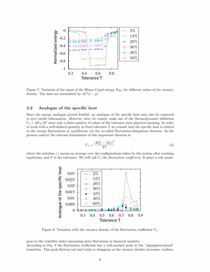
where K = 2T − 1 and the cis are ’spin-1’ variables taking the value 0 if the location i is notoccupied and 1 (resp. −1) if this location is occupied by a red (resp. blue) agent; the sums areperformed on the nearest and next nearest neighbors. This function (3) is identical to the energyof the Blume-Emery-Griffiths model [11] under the constraint that the number of sites of each type(0,±1) is kept fixed. This spin-1 model, and the Blume Capel model [12, 13] corresponding to theparticular case K = 0, have been used in particular to modelize binary mixtures and alloys in thepresence of vacancies. A more detailed analysis of the link between the Schelling model and theBlume-Emery-Griffiths model will be published elsewhere [21]. In the particular variant consideredhere, however, the dynamical rules do not lead to the minimization of such a global energy. Yet, it isclearly potentially interesting to consider this quantity ES as a surrogate of the energy. Comparedto the dynamics having ES as a Lyapunov function, the moves of satisfied agents introduce a sourceof noise which has some similarity with a thermal noise. Its amplitude may be measured by thefraction of agents who are satisfied. When starting from a random initial configuration this is higherat higher tolerance, hence the tolerance value is an indirect measure of this noise level. This givesanother motivation, different from the one already evoked, for taking the analogy between T and atemperature as a guideline for the analysis, as done in what follows. We find that the average of thesecond part of the energy ES essentially consists of a term linear with K (see appendix), so thatthe transitions are more easily located by only plotting the average of the first term of ES , Fig. 7,corresponding to the Blume-Capel part of the energy, EBC = −

∑〈i,j〉 cicj . It confirms the existence

of the two transitions previously evoked: At low tolerance its decrease occurs at the transition fromthe frozen state to the segregated one, whereas the increase observed at high tolerances correspondsto the transition to the mixed state. Such abrupt variations are characteristic of a discontinuous– in thermodynamic language ”first order” – transition. Moreover we note from Fig. 7 that as thevacancy density increases the energy varies less abruptly: This signals a change in the nature of thetransition, from discontinuous to continuous (’second order’), as will be discussed below.

7

-1

-0.8

-0.6

-0.4

-0.2

0

0.2 0.4 0.6 0.8

Nor

mal

ized

ener

gy

Tolerance T

2%

12%

28%

36%

46%

50%

Figure 7: Variation of the mean of the Blume Capel energy EBC for different values of the vacancydensity. The data are normalized by 4L2(1− ρ).

3.2 Analogue of the specific heat

Since the energy analogue proved fruitful, an analogue of the specific heat may also be expectedto give useful information. However, here we cannot make use of the thermodynamic definitionCs = dES/dT since only a finite number of values of the tolerance have physical meaning. In orderto work with a well-defined quantity at fixed tolerance T we remark that the specific heat is relatedto the energy fluctuations at equilibrium via the so-called fluctuation-dissipation theorem. In thepresent context the relevant formulation of this important theorem is:

Cs =〈E2

S〉 − 〈ES〉2

T 2(4)

where the notation 〈 〉 means an average over the configurations taken by the system after reachingequibrium, and T is the tolerance. We will call Cs the fluctuation coefficient. It plays a role analo-

0

0.005

0.01

0.015

0.02

0.025

0.03

0.3 0.4 0.5 0.6 0.7 0.8 0.9Anal

ogue

ofth

especifi

che

at

Tolerance T

2%12%28%36%42%46%60%

Figure 8: Variation with the vacancy density of the fluctuation coefficient Cs.

gous to the volatility index measuring price fluctations in financial markets.According to Fig. 8 the fluctuation coefficient has a well-marked peak at the “segregated-mixed”transition. This peak flattens out and tends to disappear as the vacancy density increases, confirm-

8

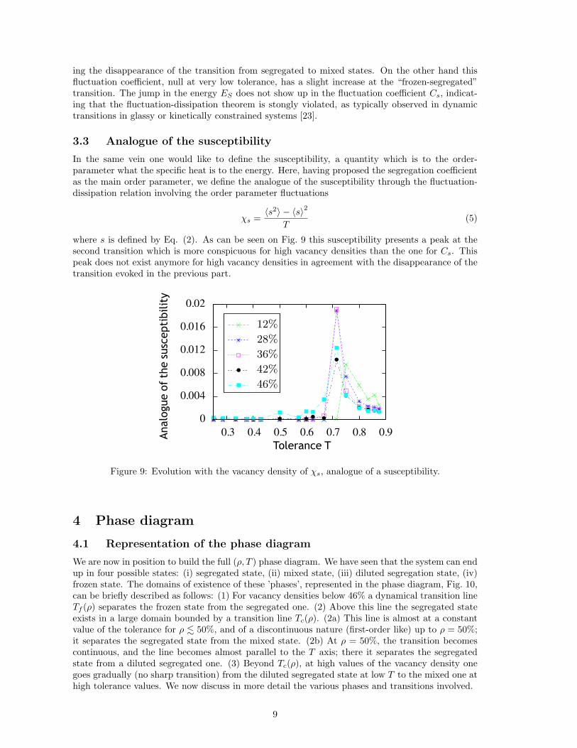
ing the disappearance of the transition from segregated to mixed states. On the other hand thisfluctuation coefficient, null at very low tolerance, has a slight increase at the “frozen-segregated”transition. The jump in the energy ES does not show up in the fluctuation coefficient Cs, indicat-ing that the fluctuation-dissipation theorem is stongly violated, as typically observed in dynamictransitions in glassy or kinetically constrained systems [23].

3.3 Analogue of the susceptibility

In the same vein one would like to define the susceptibility, a quantity which is to the order-parameter what the specific heat is to the energy. Here, having proposed the segregation coefficientas the main order parameter, we define the analogue of the susceptibility through the fluctuation-dissipation relation involving the order parameter fluctuations

χs =〈s2〉 − 〈s〉2

T(5)

where s is defined by Eq. (2). As can be seen on Fig. 9 this susceptibility presents a peak at thesecond transition which is more conspicuous for high vacancy densities than the one for Cs. Thispeak does not exist anymore for high vacancy densities in agreement with the disappearance of thetransition evoked in the previous part.

0

0.004

0.008

0.012

0.016

0.02

0.3 0.4 0.5 0.6 0.7 0.8 0.9Anal

ogue

ofth

esu

scep

tibi

lity

Tolerance T

12%

28%

36%

42%

46%

Figure 9: Evolution with the vacancy density of χs, analogue of a susceptibility.

4 Phase diagram

4.1 Representation of the phase diagram

We are now in position to build the full (ρ, T ) phase diagram. We have seen that the system can endup in four possible states: (i) segregated state, (ii) mixed state, (iii) diluted segregation state, (iv)frozen state. The domains of existence of these ’phases’, represented in the phase diagram, Fig. 10,can be briefly described as follows: (1) For vacancy densities below 46% a dynamical transition lineTf (ρ) separates the frozen state from the segregated one. (2) Above this line the segregated stateexists in a large domain bounded by a transition line Tc(ρ). (2a) This line is almost at a constantvalue of the tolerance for ρ . 50%, and of a discontinuous nature (first-order like) up to ρ = 50%;it separates the segregated state from the mixed state. (2b) At ρ = 50%, the transition becomescontinuous, and the line becomes almost parallel to the T axis; there it separates the segregatedstate from a diluted segregated one. (3) Beyond Tc(ρ), at high values of the vacancy density onegoes gradually (no sharp transition) from the diluted segregated state at low T to the mixed one athigh tolerance values. We now discuss in more detail the various phases and transitions involved.

9

Figure 10: Phase diagram of the studied Schelling model. The blue crosses correspond to thecontinuous transition between the segregated and dilute segregated states. The red triangles andpluses are the upper and lower limits of the transition between the frozen and segregated states.The red lines separate the segregated state from the mixed one. Note that the tolerance T onlytakes discrete values.

4.2 Transition frozen state / segregated state

At low tolerance there is a transition where the system abruptly switches from a frozen to a seg-regated state. The analogues of the specific heat and of the susceptibility do not have a singularbehavior in the vicinity of the transition (Fig. 8 and 9). As we have seen, this is explained by thedynamical nature of this transition – in contrast to the other transitions which are thermodynamical-like. We locate the transition by looking at the jump of the segregation coefficient, both at fixed ρ,increasing T (Fig. 3), and at fixed T , increasing ρ (Fig. 11). As the density of vacancies ρ increases,the transition occurs for lower values of the tolerance. When this density is higher than 46% thisline of transition does not exist anymore. We remark that this frozen-segregated state transitionline can fluctuate depending on the order in which the agents are chosen during the dynamics: in aninterval of tolerance and for a given vacancy density, the system may end either in a frozen state orin a segregated one. The corresponding range of tolerance is given in the appendix, Table A.4.6, foreach tested vacancy density. Let us notice that inside this frozen phase, any initial configuration,segregated or not, with randomly distributed vacancies is very close to a stationary state.

4.3 Transition segregated state/mixed state.

The segregated phase is upper bounded by a transition line where the clusters disappear and thetwo types of agents become mixed.

– This change is abrupt for vacancy densities ρ strictly smaller than 26%. Indeed, the plots ofthe segregation coefficient against the tolerance for values of ρ in this range show a jump from ∼ 1to ∼ 0 (Fig. 3).

– For 26% ≤ ρ ≤ 48%, the mixed state is reached after an intermediate state where the systemhas no dynamical stability: it can oscillate between several acceptable configurations, leading tolarge fluctuations in the segregation coefficient.

– For a small range of values, 50% ≤ ρ . 56%, the segregated states continously become mixedstates. There, the line abruptly turns downward. This area of the phase diagram, with a change inthe nature of the transition and a sudden downturn of the transition line, is more difficult to study

10

0.10.20.30.40.50.60.70.80.9

1

0 20 40 60 80

segt

rega

tion

coeffic

ient

Percentage of vacancies

1/ 8

1/ 5

2/ 7

3/ 8

1/ 2

3/ 5

2/ 3

Figure 11: Segregation coefficient for different values of the tolerance versus the vacancy density.

because of the discreteness of T values and possible finite size effects.For a given ρ the value of the tolerance at which the segregated-mixed transition occurs can belocated from the position of the peak of the analogue of either the specific heat or of the suscep-tibility (Fig. 8 and 9). In order to complete the study of this transition, we have considered thedistribution of the segregation coefficient for several values of T around the transition at differentvacancy densities (see appendix). This illustrates the three ways to go from a segregated to a mixedstate .

4.4 Transition segregated state/diluted segregation state.

As just mentioned, the boundary Tc(ρ) of the segregated phase becomes weakly dependent onthe vacancy density ρ when ρ becomes slightly larger that 50%. To locate the transition line weplot for several values of T the variation with ρ of the segregation coefficient Cs (Fig. 11), and ofthe analogue of the susceptibility χs (see appendix Fig. A.4). At high vacancy densities, beyondthe transition line, the nature of the phase is different at high and low tolerances. As we haveseen, at high tolerance values there is a mixed state, whereas at low tolerance one finds a dilutedsegregation state that leads to very small segregation coefficients. Indeed, at high ρ (> 0.592746,the percolation threshold [18]), the high probability of percolation of vacancies prevents the formingof large clusters. In this high vacancy density domain, we do not find any sharp transition from thediluted segregated state to the mixed one, but only a gradual change as the tolerance increases.

4.5 Comparison with the Blume-Capel phase diagram.

It is instructive to compare the phase diagram with the one of the Blume-Capel model [12, 13]evoked above (see appendix). For this model a transition line separates a ferromagnetic (segre-gated) phase from a domain where one goes gradually from a paramagnetic (mixed) phase to aphase where the vacancies predominate. This line changes as well its nature from discontinuousto continuous. However, it is the ferromagnetic-paramagnetic transition which is second order,whereas the segregated-mixed transition is first order-like (the change is abrupt). Conversely, thetransition between the ferromagnetic and the high vacancy density phases is first order, whereasthe corresponding transition in the Schelling model is continuous.

11

Conclusion

We analyzed a variant of the Schelling model from a physical point of view. We have introduced ameasure of segregation and analogues of physical quantities such that the fluctuation coefficient andthe susceptibility where, remarkably, the analogy between the tolerance and the temperature provesfruitful. These quantities allowed to identify the different phases of the system and characterize thetransitions between them (thermodynamical or dynamical like, discontinuous or continuous). Themain results have been summarized as a phase diagram in the (ρ, T )-plane where ρ is the vacancydensity and T the tolerance. Considering larger neighborhoods would allow to have a larger set ofvalues for T and approach a continuous model. A more precise location of the phase boundaries, ifneeded, would require computationally costly simulations of larger network sizes.We have seen in particular that the segregated phase occupies a large domain (up to a tolerance Tas high as 3/4), confirming Schelling’s intuition on the genericity of the segregation phenomenon.The abrupt transition from a mixed to a segregated state could be interpreted as the tipping point– more precisely the rapid ethnic turnover – observed and studied by social scientists [24]. Besides,the diluted segregation state might be relevant for low-density suburban areas. The frozen statewould probably be unstable in a more realistic model allowing for migratory flows of discontentagents to other cities.The tools and methods presented here could be used to study other Schelling-like models. Clearlyfuture works should focus on models grounded on empirical data and where the agent decision rulestake into account relevant socio-economic factors [4]. Yet it is known from a large body of workin statistical physics that one needs also to explore more widely the space of models in order toidentify what makes a particular behavior specific or generic. As already mentioned our goal herewas to provide generic tools for the analysis of models of socio-dynamics. The variant of Schelling’ssegregation model we have studied as a test of our approach has the advantage of being identicalor very close to variants already studied in the literature and to allow links with known - and nontrivial - spin models.

Acknowledgements

LG is supported by a fellowship from the French Ministere de l’Enseignement Superieur et de laRecherche, allocated by the Ecole doctorale de Physique de l’UPMC – ED 389. JV and JPN areCNRS members. This work is part of the project ’DyXi’ supported by the SYSCOMM program ofthe French National Research Agency (grant ANR-08-SYSC-008).

References

[1] Schelling T (1971) Dynamic Models of Segregation. J Math Sociol 1: 143–186.

[2] Schelling T (1978) Micromotives and Macrobehavior (W. W. Norton, NewYork).

[3] Vriend N and Pancs R (2007) Schelling’s spatial proximity model of segregation revisited. JPubl Econ 91:1–24.

[4] Clark W and Fossett M (2008) Understanding the social context of the Schelling segregationmodel. Proc Natl Acad Sci USA 105:4109–4114.

[5] Vinkovic D and Kirman A (2006) A physical analogue of the Schelling model. Proc Natl AcadSci USA 103:19261–19265.

[6] Stauffer D and Solomon S (2007) Ising, Schelling and self-organising segregation. Eur Phys JB 57:473–479

[7] Marsili M, Dall’Asta L and Castellano C (2008) Statistical physics of the Schelling model ofsegregation. J Stat Mech L07002.

12

[8] Odor G (2008) Self-organizing, two-temperature Ising model describing human segregation IntJ Modern Phys C 19, 3:393-398]

[9] Castellano C, Fortunato S and Loreto V (2007) Statistical physics of social dynamics.arXiv:0710.3256v1 [physics.soc-ph], to appear in Rev Modern Physics (2009).

[10] Adaptive Agents, Intelligence and Emergent Human Organization: Capturing ComplexityThrough Agent-Based Modeling (2002) Proc. of the Arthur M. Sackler Colloquium Proc NatlAcad Sci USA 99, suppl.3.

[11] Blume M, Emery V J and Griffiths R B (1971) Ising model for the λ transition and phaseseparation in He3-He4 mixtures. Phys Rev A 4:1071–1077 .

[12] Blume M (1966) Theory of the first-order magnetic phase change in UO2. Phys Rev 141:17–524.

[13] Capel H W (1966) On the possibility of first-order phase transitions in Ising systems of tripletions with zero-field splitting. Physica 32:966–987.

[14] Weiss H, Singh A and Vainchtein D (2007) Schelling’s segregation model: Parameters, scaling,and aggregation. arXiv 0711.2212v1 [nlin.AO].

[15] Grauwin S and Jensen P (2008) ENS Lyon, report.

[16] Bray A J (1994) Theory of phase-ordering kinetics. Adv Physics 43:357–459.

[17] Vriend N J, Fagiolo G and Valente M (2007) Segregation in Networks. J Economic Behaviorand Organization 64(3-4):316–336.

[18] Stauffer D and Aharony A (1992) Introduction to Percolation Theory (Taylor and Francis,London).

[19] Hoshen J and Kopelman R (1976) Percolation and cluster distribution. i. Cluster multiplelabeling technique and critical concentration algorithm. Phys Rev B 14:3438–3445.

[20] Burkhardt T W and van Leeuwen J M J Eds. (1982) Real-Space Renormalization (Springer-Verlag, New York).

[21] Gauvin L, Nadal J-P and Vannimenus J (2009) In preparation.

[22] Stanley H E (1971) Introduction to Phase Transitions and Critical Phenomena (ClarendonPress, Oxford).

[23] Ritort F and Sollich P (2003) Glassy dynamics of kinetically constrained models Adv Physics52:219–342.

[24] Wilson W, Taub R (2007) There Goes the Neighborhood: Racial, Ethnic, and Class Tensionsin Four Chicago Neighborhoods and Their Meaning for America (Vintage Book, New York).

13

A Appendix

A.1 Numerical simulations

All the simulations except on the Fig. 1 were performed on a 50 × 50 lattice. We tested all themeaningful values of the tolerance T at even values of the vacancy percentage ρ. With this choicefor ρ, the number of vacancies and of agents of two colors are exactly equal to the integers ρ ∗ L2

and L2(1 − ρ). To take only even values of the vacancy percentage ρ also allows to moderate thecomputational cost.

A.2 Real-Space Renormalization procedure

To identify clusters at a larger scale, we performed the following renormalization procedure. Wedivide the lattice into squares of 4 sites. On each of these little squares, we look at the bottom rightsite :

– If this site and its neighborhood comprise a majority of blue (resp. red) agents, the 2 × 2square is replaced by a (single) blue (resp. red) agent.

– If this site and its neighborhood consist of a majority of vacancies, the 2×2 square is replacedby a vacancy.

– If there is no majority, the 4-site square is replaced by an agent of the same type as the bottomright site (or by a vacancy if that site is empty).

A.3 Contact with spin-1 models

A.3.1 Energy of Schelling models

For completeness we present here a correspondence, discussed elsewhere [21], between Schellingsegregation models and spin-1 models.One can associate to each site i of the lattice a spin variable ci, taking the value 0 if the location isnot occupied, and 1, resp. −1, for red, resp. blue, occupied sites. With these ’spin-1’ variables thesatisfaction condition for location i (including the case where i is vacant) can be written as:

ci∑j∈(i)

cj + (2T − 1)c2i∑j∈(i)

c2j ≥ 0 (6)

where j ∈ (i) means j belonging to the neighborhood of site i. This suggests to define, as ananalogue of the energy,

ES = −∑〈i,j〉

cicj −K∑〈i,j〉

c2i c2j , (7)

where K = 2T − 1 (−1 ≤ K ≤ 1), and the index S stands for “Schelling”.For the Schelling original model, as well as for other variants where only unsatisfied agents canmove, one can show [21] that the energy ES is indeed a Lyapunov function, that is a quantity whichdecreases with time during the dynamics, driving the system towards a fixed point. Note that theenergy is not proportional to the global utility U =

∑i ui, where ui is 1 if agent i is satisfied, and

0 otherwise.

This function ES , (3), is identical to the energy of the Blume-Emery-Griffiths model [11] underthe constraint that the number of sites of each type (0,±1) is kept fixed. This spin-1 model, andthe Blume Capel model [12, 13] corresponding to the particular case K = 0, have been used in

14

particular to modelize binary mixtures and alloys in the presence of vacancies. In the standardversions of these models, the energy contains the additional term D

∑i ci

2 (the sum being overall the sites), so that the total number of vacancies is fixed only in average through the Lagrangemultiplier D:

EBEG = −∑〈i,j〉

cicj −K∑〈i,j〉

c2i c2j +D

∑i

ci2 (8)

The limit D → −∞ corresponds to the absence of vacancies, i.e. the Ising model. Large positive Dcorresponds to high vacancy densities. The term D does not appear in the energy of the Schellingmodel, not because it corresponds to D = 0, but because the density of vacancies is fixed. Thefact that ES is a Lyapunov function for the Schelling model where only unsatisfied agents move,means that such a model is equivalent to a Blume-Emery-Griffiths model without thermal noise(zero temperature), and under kinetic constraints (e. g., no direct exchange between two agents ofdifferent colors is allowed).

The standard order parameters for these spin-1 systems are the magnetization (1/N)∑

i ciand the quadrupole moment, (1/N)

∑i c

2i , but here these quantities which are, respectively, the

difference between the total numbers of agents of different colors, and the density of occupied sites,are kept fixed by construction in the Schelling model. .

A.3.2 Blume-Capel model: phase diagram

A striking similarity exists between the phase diagram in the (ρ, T ) plane of the variant of theSchelling model studied here, and the one of the Blume-Capel model [12, 13] in the (D,T ) plane –where T is the temperature and D the parameter fixing in average the vacancy density.The Blume-Capel phase diagram, computed for the Moore neighborhood, is shown on Fig A.1, andshould be compared with the one on Fig 10. The red part of the transition line corresponds to afirst-order (discontinuous) transition, and the blue part to a second-order (continuous) transition.Below the transition line the system is in an ordered, ferromagnetic, state. Above the transitionline, at low and medium values of D, one finds the unordered, paramagnetic, phase, and at large Dand low temperature, a vacancy dominated phase. In the latter phase, the typical configurationsare not strictly comparable to the ones of the corresponding phase in the Schelling model: in thespins models, the clusters are compact whereas it is not the case in the Schelling model. In theBlume-Capel model there is no frozen phase, because there is no constraint on the dynamics.

The transition line in the Blume-Capel model, shown on Fig A.1, has been built up by plottingfor fixed temperature T (resp. fixed D depending on the area of the diagram dealt with) themagnetization versus D (resp. T ) for three different sizes, and by looking at the value of D (resp.T ) corresponding to the intersection of the three curves.

15

1

2

3

4

5

-8 -6 -4 -2 0 2 4 6

kbT

D

2nd order1st order

Figure A.1: Phase Diagram of the Blume Capel model with first and second neighours interactions(Moore neighborhood). The simulations were performed using the Heat Bath algorithm.

A.4 Complementary analysis of the segregation model

A.4.1 Density of satisfied agents

The density of satisfied agents is a good indicator of the convergence of the system towards itsstationary state (whenever it exists), in which the fraction of satisfied agents is constant. Fig. A.2shows the evolution of the density of satisfied agents for a case with low vacancy density ρ = 5%and moderate tolerance T = 0.5. We note that, in the unstable part of the phase diagram (close toTc at 26% ≤ ρ . 50%), the density of satisfied agents is stationary: this shows that, more generally,the convergence of the fraction of satisfied agents does not guarantee that the system itself hasreached a steady state.

0.6

0.7

0.8

0.9

1

0 10 20 30Den

sity

ofsatisfied

agen

ts

Steps

Figure A.2: Evolution of the proportion of satisfied agents versus the number of steps for ρ = 5%and T = 0.5. About 60% of the agents are initially satisfied. The dynamics quickly allows theagents to be almost all satisfied, after only 10 steps the density of satisfied agents is very close to1. It increases slowly afterwards, with small fluctuations due to the possibility for satisfied agentsto keep moving.

16

A.4.2 Unwanted vacancies

The variation with the tolerance of the unilaterally unwanted density of vacancies ρ (Fig.A.3) con-firms that the mixed situation observed for low values of T is due to the dynamics. The agents

0

0.2

0.4

0.6

0.8

1

0.2 0.4 0.6 0.8

Vaca

ncy

Den

sity

ρ

Tolerance T

ρ = 2%

ρ = 6%

ρ = 12%

ρ = 18%

Figure A.3: Density ρ of vacancies where no type of agent would be satisfied, for several values ofthe vacancy density.

reject all the empty spaces, consequently the system cannot evolve. At tolerances corresponding tothe frozen state - segregated state transition, the situation reverses. All vacancies are acceptablefor at least one type of agents.

A.4.3 Analogue of the susceptibility

The analogue of the susceptibility for the Schelling model is given by:

χs =〈s2〉 − 〈s〉2

T, (9)

where the notation 〈 〉 means an average over the configurations taken by the system after reachingequibrium, and T is the tolerance. These fluctuations allow to locate the transition at fixed tolerance

0

0.01

0.02

0.03

0.04

0.05

0.06

0 10 20 30 40 50 60 70 80

Anal

ogue

ofth

esu

scep

tibi

lity

Percentage of vacancies

1/ 5

2/ 5

4/ 7

5/ 8

Figure A.4: Analogue of the susceptibility for different values of the tolerance versus the vacancydensity. The averages have been computed on 30000 simulations after equilibrium.

17

T as the density of vacancies increases.

A.4.4 Blume-Emmery-Griffiths energy vs Blume-Capel energy

We have shown that the appropriate energy related to the Schelling model is the Blume-Emmery-Griffiths energy at constant number of sites of each type (red and blue agents, and vacancies),defined by (7). However we find that the analysis of the transitions can be done as well from theBlume-Capel energy, that is here, since the number of sites of a given type is fixed (no D-term):

EBC = −∑〈i,j〉

cicj (10)

Note that in the absence of vacancies, ci = ±1 so that EBC would reduce to the standard Isingenergy. One finds that the fluctuation coefficient obtained with the Blume-Capel energy, defined byC ′s = 〈E2

BC〉−〈EBC〉2T 2 and shown on Fig A.5, is very similar to the one obtained from the Schelling

energy ES . Actually, in the evolution of the mean of the total energy ES , shown on Fig. A.6, onerecognizes the contribution from the Blume-Capel energy EBC (shown on Fig. 7), simply increasedby an additional term linear in K = 2T − 1. These observations can be explained by the fact thatthe difference between these two energies is proportionnal to the numbers of pairs of occupied sitesof which the fluctuations are weak. Indeed, one observes that the vacancies remain approximativelyuniformly distributed. This comes from the fact that each agent searches for locations where thenumber of unlike neighbors is inferior to a given proportion of the number of neighbours. Note thatthe vacancies would not be uniformly placed if each agent wanted less than a fixed number of unlikeneighbors, as considered in [14].

0

0.005

0.01

0.015

0.02

0.025

0.03

0.3 0.4 0.5 0.6 0.7 0.8 0.9

Anal

ogue

ofth

especifi

che

at

Tolerance T

2%12%28%36%42%46%60%

Figure A.5: Variation of the analogue of thespecific heat obtained from the Blume-Capel en-ergy for different values of the vacancy density.

-1.5

-1

-0.5

0

0.5

0.2 0.4 0.6 0.8

Nor

mal

ized

ener

gy

Tolerance T

2%

12%

28%

36%

46%

50%

Figure A.6: Variation of the mean of the energyES for different values of the vacancy density.The data are normalized by 4L2(1− ρ).

A.4.5 Segregation coefficient

In order to get more information about the segregated state-mixed state transition, it is instructiveto look at the distribution of the segregation coefficient < s > in the vicinity of the transition (FigsA.7 and A.8). The distributions have been obtained from 30000 calculations of the segregationcoefficient.At vacancy density ρ lower than 26%, the transition is well marked. This distribution is centerednear 0 at the transition point whereas it is centered near 1 at the closest inferior value of thetolerance. Indeed, the distributions of the segregation coefficient for successive tolerances aroundthe transition are clearly separated for the vacancy density ρ = 24% (left Fig. A.7).As ρ increases, the transition is achieved via an intermediate state. One distinguishes three kinds ofdistributions (Figs. A.7, right and A.8, left) which are centered around a very small value (∼ 0.2),peaked close to 1, or centered around an intermediate value. The latter case corresponds to abroader distribution.

18

0

0.01

0.02

0.03

0.04

0 0.2 0.4 0.6 0.8 1

Freq

uenc

yof

occu

renc

eT = 5 / 7T = 3 / 4

<s>

0

0.05

0.1

0.15

0.2

0 0.2 0.4 0.6 0.8 1

T = 5 / 7T = 3 / 4T = 2 / 3

<s>

Figure A.7: Distributions (normalized by the number of measures) of the segregation coefficient forρ = 24% and ρ = 28%.

0

0.01

0.02

0.03

0.04

0.05

0 0.2 0.4 0.6 0.8 1

Freq

uenc

yof

occu

renc

e

T = 5 / 7T = 3 / 4T = 2 / 3

<s>

0

0.002

0.004

0.006

0.008

0.01

0.012

0 0.2 0.4 0.6 0.8 1

T = 5 / 7T = 3 / 4 T = 2 / 3

T = 5 / 8

<s>

Figure A.8: Distribution of the segregation coefficient for ρ = 44% and ρ = 50%.

Once the vacancy density is greater than 50%, all the distributions of the segregation coefficientbegin to blend together (see Fig A.8, right). This confirms that the increase in the vacancy densityis accompanied by a change in the nature of the transition between 46% and 50%, which becomescontinuous.

19

A.4.6 “Frozen-segregated” transition line

The transition line between the frozen and the segregated states has been determined by locatingthe jump of the segregation coefficient < s > from ∼ 0 to ∼ 1. The initial configuration and theorder of choice of the agents, when the dynamics is applied, create fluctuations on the limit betweenthe two states. Actually, for some sets of parameters (ρ, T ), the system may end either in blockedor in segregated configurations depending on the order of choices of the agents. One cannot excludethat this unstable domain is due to finite size effects, hence disappearing in the infinite networksize limit. However, it is not surprising to find such a metastability effect close to a discontinuoustransition.

ρ 2% 4% 6% 8% 10% 12% 14% 16%T 1

212

25 −12

38 −37

38

38

38

13 −38

ρ 18% 20% 22% 24% 26% 28% 30% 32%

T

13 −38

13

14 −13

14 −13

15 −14

15 −14

15

15

ρ 34% 36% 38% 40% 42% 44% 46%T 1

515

15

15

16 −15

18 −15

18

Table 1: ”Frozen state-segregated state“ transition line. The limits between which the system mayend in a frozen state or segregated state depending on the order of the dynamics are obtained byperforming 100 tests on which we look at the percentage of ”frozen states”. If for given T and ρ,the percentage of frozen states (resp. segregated states) is very high (> 95%), we consider that thecorresponding equilibrium configuration is a frozen one (resp. segregated).

20