Phase-Coded-Linear-Frequency- Modulated Waveform · PDF filewith the best mental and physical...

Phase-Coded-Linear-Frequency-

Modulated Waveform for a Low Cost

High Resolution Radar System

by Melin Ngwar

A thesis

presented to the Department of Electronics

in fulfillment of the

thesis requirement for the degree of

Masters of Applied Science

Ottawa-Carleton Institute for Electrical Engineering

Department of Electronics

Carleton University

Ottawa, Ontario

Copyright ©2010, Melin Ngwar

1*1 Library and Archives Canada

Published Heritage Branch

395 Wellington Street OttawaONK1A0N4 Canada

Bibliothgque et Archives Canada

Direction du Patrimoine de I'gdition

395, rue Wellington OttawaONK1A0N4 Canada

Your file Votre reference ISBN: 978-0-494-71567-3 Our file Notre reference ISBN: 978-0-494-71567-3

NOTICE: AVIS:

The author has granted a nonexclusive license allowing Library and Archives Canada to reproduce, publish, archive, preserve, conserve, communicate to the public by telecommunication or on the Internet, loan, distribute and sell theses worldwide, for commercial or noncommercial purposes, in microform, paper, electronic and/or any other formats.

L'auteur a accorde une licence non exclusive permettant a la Bibliotheque et Archives Canada de reproduire, publier, archiver, sauvegarder, conserver, transmettre au public par telecommunication ou par I'lntemet, preter, distribuer et vendre des theses partout dans le monde, a des fins commerciales ou autres, sur support microforme, papier, electronique et/ou autres formats.

The author retains copyright ownership and moral rights in this thesis. Neither the thesis nor substantial extracts from it may be printed or otherwise reproduced without the author's permission.

L'auteur conserve la propriete du droit d'auteur et des droits moraux qui protege cette these. Ni la these ni des extraits substantiels de celle-ci ne doivent etre imprimes ou autrement reproduits sans son autorisation.

In compliance with the Canadian Privacy Act some supporting forms may have been removed from this thesis.

Conformement a la loi canadienne sur la protection de la vie privee, quelques formulaires secondaires ont ete enleves de cette these.

While these forms may be included in the document page count, their removal does not represent any loss of content from the thesis.

Bien que ces formulaires aient inclus dans la pagination, il n'y aura aucun contenu manquant.

•+•

Canada

AUTHOR'S DECLARATION

I hereby declare that I am the sole author of this thesis. This is a true copy of the thesis,

including any required final revisions, as accepted by-my examiners.

I understand that my thesis may be made electronically available to the public.

11

Abstract

Low cost Radar Systems are difficult to realize due to their high peak power requirement.

High output power implies the need for unconventional and expensive power amplifiers such

as magnetrons and travelling wave tubes. Peak output power is reduced by increasing the

pulse width of the transmitted signal with minimum output power obtained from a

continuous waveform or infinite pulse width. However, the drawback to increasing the pulse

width is deterioration in resolution. This thesis uses pulse compression to achieve the

required resolution. It combines two compression schemes: phase modulation and frequency

modulation. Phase modulation is used to reject ambiguous targets while frequency

modulation is used to achieve the finest resolution. Convolution of the phase modulated and

frequency modulated waveforms yields a waveform which has the fine resolution property of

the frequency modulated signal and the ambiguous target rejection property of the phase

modulated signal. Target detection is done by correlation, and both types of pulse

compression schemes have an auto-correlation response which approximates a delta function.

Convolution is the only scheme which preserves the delta function auto-correlation response

of the resulting waveform upon combination of the frequency and phase modulated signals.

The Radar System demonstrated in this thesis also has a speed detection capability and this

can be used to separate moving targets from stationery ones. Measured target speed is

directly proportional to the frequency (Doppler) shift caused by moving targets and is

obtained in this thesis by observing the phase shift over successive echoes. Since serial

Doppler processing is done on correlated values, it has a higher CNR at the Doppler

frequency than parallel Doppler processing performed on the received signal.

iii

Acknowledgements

The guidance given by my supervisor, Professor Jim Wight has been-invaluable to my

research efforts. His aid in the acquisition of Research grants and facilities has provided me

with the best mental and physical environment throughout the course of this project.

All work done during the course of this research has been carried out at the D.Roy / T.Roy

Advanced Sensor Processing Lab. I will like to acknowledge D-TA systems for financially

supporting this research and providing the equipment required for experimental evaluation. I

will also like to thank Pier Bortot, CTO of D-TA Systems for his invaluable assistance in all

aspects of design and implementation.

Financial Support for this thesis was provided by the Department of Electronics at Carleton

University, Faculty of Graduate Studies at Carleton University, Ontario Center of Excellence

and D-TA Systems.

IV

Table of Contents

AUTHOR'S DECLARATION ii

Abstract iii

Acknowledgements iv

Table of Contents v

List of Figures vii

List of Tables ix

List of Abbreviations x

Chapter 1 Introduction to Low Cost Radar 1

1.1 Description of Thesis Objectives 1

1.2 Waveform Design and Processing 1

1.3 Doppler Processing 2

1.4 Radar Channel 3

1.5 Thesis Overview 5

Chapter 2 Radar Overview and System Hardware 6

2.1 Background on Radar Concepts 6

2.2 Background on System Hardware 12

2.3 Specifications 15

2.4 Chapter Summary 18

Chapter 3 Waveform Design 19

3.1 Phase-Coded Pulse Compression 19

3.2 Frequency Modulation Compression 21 v

3.3 Phase-Coded-Linear-FM 24


Chapter 4 Radar Simulation in Matlab 30

4.1 Transmitter 30

4.2 Channel 33

4.3 Receiver Processing 35

4.4 Simulated Serial Vs Parallel Processing 43


Chapter 5 Implementation and Testing 47

5.1 Real Time Processing 47

5.2 Transmitted Spectrum 48

5.3 Resolution and Power Verification 51

5.4 Doppler Verification 56

5.4.1 Doppler Test Setting 56

5.4.2 Doppler Test Results 58

5.5 Tested Serial Vs Parallel Radar Processing 61


Chapter 6 Discussion and Conclusion 64

6.1 Discussion 64

6.2 Conclusion 66

Appendix A Antenna Measurements 70

vi

List of Figures

Figure 2.1: Generalized Receiver Chain 9

Figure 2.2: Change in SNR with probability of Detection for various probabilities of false

alarm [4] 9

Figure 2.3: Probability distribution function for Swerling targets 11

Figure 2.4: Plot of Additional SNR with Probability of detection for Swerling 1 - 4 [4] 12

Figure 2.5: Block Diagram for D-TA 2300 14

Figure 2.6: Block Diagram for D-TA 3290 (RF Up-converter) 15

Figure 2.7: Radar Geometry 15

Figure 3.1: Auto-Correlation of MLS with n=20 and N = 1,048,575 truncated to 640bits per

PRI 21

Figure 3.2: Auto-Correlation of linear-FM chirp 24

Figure 3.3: Auto-Correlation of convolved phase modulated and linear-FM signal 27

Figure 3.4: Normalized peak cross-correlation value over successive pulses 28

Figure 4.1: Block Diagram for the transmitter 31

Figure 4.2: Spectrum of triangular FM chirp 31

Figure 4.3: Spectrum of phase modulated signal 32

Figure 4.4: Spectrum of phase-coded-linear-frequency-modulated signal 32

Figure 4.5: Block Diagram for Radar Channel 35

Figure 4.6: Block Diagram for Receiver Correlation Processing 37

Figure 4.7: Simulated Auto-Correlation Response for a Swerling III or IV target 37

Figure 4.8: Simulated Auto-Correlation Response for a Swerling I or II targets 38 vii

Figure 4.9: Doppler Spectrum for Swerling I target 40

Figure 4.10: Doppler Spectrum for Swerling III target 40

Figure 4.11: Doppler Spectrum for Swerling II target 41

Figure 4.12: Doppler Spectrum for Swerling IV target 41

Figure 4.13: Doppler Spectrum obtained from 1024 point FFT at clutter range bin 42

Figure 4.14: Doppler Spectrum of Serial process for non-fluctuating target 45

Figure 4.15: Doppler Spectrum of Parallel process for non-fluctuating target 45

Figure 5.1: Block Diagram of Baseband Processor 48

Figure 5.2: Output of D-TA 2210 as seen on Spectrum Analyzer 49

Figure 5.3: Output of D-TA 3290 as seen on Spectrum Analyzer 49

Figure 5.4: D-TA 2300 (on right) and RF transceiver (on left) 50

Figure 5.5: Circular polarized antenna (on left) and Horn antenna (on right) 50

Figure 5.6: Plot of Auto-correlation against range for phase-coded-linear-FM waveform 53

Figure 5.7: Plot of Auto-correlation against range for phase-coded waveform 54

Figure 5.8: Plot of Auto-correlation against range for linear-FM waveform 54

Figure 5.9: Cross-Section of Powermax fan 58

Figure 5.10: Doppler spectrum at target range bin for fan rotating at 1220rpm 59

Figure 5.11: Doppler spectrum at target range bin for fan rotating at 1517rpm 60

Figure 5.12: Serial and Parallel Doppler Spectrum of fan at 1220rpm 62

Figure 5.13: Serial and Parallel Doppler Spectrum of fan at 1517rpm 62

Figure 6.1: Elevation plane Gain measurement for the H-1734 antenna at 1.5GHz 70

Figure 6.2: Azimuth plane Gain measurement for the H-1734 antenna at 1.5GHz 70

viii

List of Tables

Table 5.1: Table of Normalized Auto-correlation values L 55

Table 5.2: Tested and Simulated Serial and Parallel carrier to noise ratios at different

frequencies 63

IX

List of Abbreviations

ADC Analog to Digital Converter

AWGN Additive White Gaussian Noise

CNR Carrier to Noise Ratio

DAC Digital to Analog Converter

dB decibels

FIFO First in First out buffer

FFT Fast Fourier Transform

FM Frequency Modulation

IF Intermediate Frequency

LFSR Linear Feedback Shift Register

LOS Line of Sight

MLS Maximum Length Sequence

NCO Numerically Controlled Oscillator

PLS Partial Length Sequence

PM Phase Modulation

PRI Pulse Repetition Interval

PRF Pulse Repetition Frequency

x

Chapter 1

Introduction to Low Cost Radar

1.1 Description of Thesis Objectives

Most existing radar systems are quite expensive due to their high transmitter power

requirement. Since transmission in pulsed radar only occurs for a small fraction of the PRI, a

high power level is required to achieve a reasonable maximum range. Regular power

amplifiers are insufficient to provide the required power levels, hence the need for TWTs and

Magnetrons which are quite costly. The solution to this problem is to increase system gain by

transmitting for 100% of the PRI or using a continuous waveform. In this way, the average

power (Pav) can be maintained by decreasing the peak power (Pt) and increasing the pulse

width (T) as derived from the equation 1.0.

p-»=%, 0.0)

The purpose of this thesis is to design and test a waveform which requires low power, has

high resolution, rejects ambiguous targets and detects moving targets with a high carrier to

noise ratio. The proposed waveform and processing is implemented on sensor interfaces built

by D-TA Systems.

1.2 Waveform Design and Processing

Pulse compression is used to spread the transmitted energy and at the same time achieve

the same resolution as a narrow pulse. The most common pulse compression schemes are

phase-coded and frequency modulated waveforms. This thesis examines the said

compression schemes and proposes a waveform which has both phase coding and frequency

modulation properties. Range resolution is the minimum detectable separation between two

targets at the same bearing. Both frequency and phase modulated waveforms have finer range

resolution than pulsed waveforms for a particular bandwidth. However, the resolution of

phase modulated signals is limited by the IF bandwidth while the optimum achievable

resolution of a frequency modulated signal is limited by the sampling frequency. This implies

that FM signals can achieve much finer resolution than phase modulated signals. FM signals

are however, periodic meaning ambiguous targets are not rejected. Phase modulated signals

are derived from truncated random sequences with long periods. The implication is PM

signals can reject ambiguous targets by cross-correlation. The proposed combined scheme

possesses the fine resolution property of the FM signal and ambiguous target rejection

property of the PM signal. Target range is obtained by auto-correlation of the transmitted

signal and its echo. Correlation compresses the echo such that even signals below the noise

floor appear as a peak at the appropriate range bin.

1.3 Doppler Processing

For Doppler detection, typical radar systems detect the phase of the echo over successive

pulses and use a bank of filters (FFT) to detect the Doppler frequency of the target. For

echoes below the noise floor, a huge FFT length or number of filters is required to obtain the

Doppler frequency. Doppler detection which is done by processing the auto-correlation phase

is called serial Doppler processing because the range is first detected by auto-correlation

before Doppler is processed. This way the FFT length required to detect the Doppler

frequency is much smaller and hence a more efficient use of resources. The drawback to

2

system processing in this fashion is greater latency as range and Doppler processing are done

sequentially as opposed to systems which process in parallel. Parallel Doppler processing

refers to systems which detect the Doppler shift and range simultaneously. While parallel

processing might be faster than serial processing, the resulting carrier to noise ratio at the

Doppler frequency is often smaller than that obtained from a serial process. This is because

serial processes extract the signal from the noise before Doppler processing while parallel

processes do not.

1.4 Radar Channel

Accurate values of range for low angle targets are often difficult to determine for most

radars due to the presence of multipath. In maritime environments most of this error is

manifested in the elevation because the echo's image occurs only in elevation even though

residual cross-talk can cause manifestation of this error in the azimuth [1]. With knowledge

of the delay between the line of sight and multipath component, compression parameters can

be chosen such that the line of sight and multipath components are separated by correlation.

In this way the radar system acts as a Rake receiver without recombination as the radar

receiver is only interested in the path of minimum delay. Poor elevation accuracy is quite

detrimental to system performance because it limits the Radar's ability to implement

effective countermeasures to impending threats. For example missiles approaching a ship

travel at very high speed thus they should be detected with acceptable accuracy using the

fewest number of pulses. The radar system discussed in this paper is tailored to operate in the

presence of both land and sea clutter. Land clutter has a Doppler shift around zero while sea 3

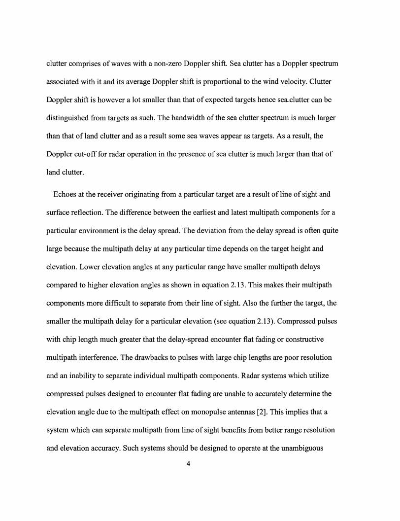
clutter comprises of waves with a non-zero Doppler shift. Sea clutter has a Doppler spectrum

associated with it and its average Doppler shift is proportional to the wind velocity. Clutter

Doppler shift is however a lot smaller than that of expected targets hence seaxlutter can be

distinguished from targets as such. The bandwidth of the sea clutter spectrum is much larger

than that of land clutter and as a result some sea waves appear as targets. As a result, the

Doppler cut-off for radar operation in the presence of sea clutter is much larger than that of

land clutter.

Echoes at the receiver originating from a particular target are a result of line of sight and

surface reflection. The difference between the earliest and latest multipath components for a

particular environment is the delay spread. The deviation from the delay spread is often quite

large because the multipath delay at any particular time depends on the target height and

elevation. Lower elevation angles at any particular range have smaller multipath delays

compared to higher elevation angles as shown in equation 2.13. This makes their multipath

components more difficult to separate from their line of sight. Also the further the target, the

smaller the multipath delay for a particular elevation (see equation 2.13). Compressed pulses

with chip length much greater that the delay-spread encounter flat fading or constructive

multipath interference. The drawbacks to pulses with large chip lengths are poor resolution

and an inability to separate individual multipath components. Radar systems which utilize

compressed pulses designed to encounter flat fading are unable to accurately determine the

elevation angle due to the multipath effect on monopulse antennas [2]. This implies that a

system which can separate multipath from line of sight benefits from better range resolution

and elevation accuracy. Such systems should be designed to operate at the unambiguous

4

range for low angles of elevation and targets within the limits of operation will achieve

superior performance.

1.5 Thesis Overview

Chapter 1 provides a description of the Radar problem and an overview of the Design

methodology. Chapter 2 describes the Radar concepts utilized in the waveform design and

processing. Chapter 2 also provides a background on the system hardware required for

waveform implementation. Chapter 3 is a detailed examination of the Design process used to

generate the proposed phase-coded-linear-FM signal. Chapter 4 shows the simulated

performance of the proposed waveform under channel effects while Chapter 5 shows the

tested results. Finally, Chapter 6 provides a comparison of the expected, simulated and tested

results.

5

Chapter 2

Radar Overview and System Hardware

2.1 Background on Radar Concepts

Radio Detection and Ranging (RADAR) is a system that determines the location of objects

by transmitting a signal and detecting its echo. A portion of the transmitted signal that

reaches the target is reflected in all directions and the radar antenna collects the returned

energy in its direction [2]. The distance from Radar to target (R) as shown in equation 2.1 is

determined by measuring the time between the transmitted signal and its echo reception (At).

R = c-Y (2-D

Where c is the speed of light. Target azimuth is obtained by rotating the antenna about a

vertical axis while elevation is obtained by determining the angle of arrival from beam

processing. Moving targets apply a frequency shift (Doppler effect) to the transmitted signal

which is proportional to the relative velocity between the Radar and target. The receiver uses

these frequency shifts to distinguish moving targets from stationery ones. The maximum

expected (unambiguous) range determines the maximum pulse length or pulse repetition

interval (PRI). The maximum pulse rate is the inverse of the PRI and is called the pulse

repetition frequency (PRF). Echoes which take longer than the PRI to arrive represent

ambiguous targets and they cause faulty range measurements if they aren't rejected, because

the receiver doesn't know which transmitted pulse they correspond to. Unambiguous range is

given by equation 2.2.

6

RuNAMBIG = 2^pRp (2-2)

Pulse compression utilizes frequency or phase modulation for compression of the transmitted

signal. Longer pulses have higher energy and compression ensures that range resolution is

not affected. Range resolution is given by equation 2.1, where At is the pulse width for

rectangular pulses and the chip width in the case of phase modulated pulses. The maximum

range is determined by the minimum signal the receiver can detect and is given by equation

2.3.

n 4 __ PtGtGraX ,ry ^v nmax — (Ajr^p \A-J)

v*n) ^rjnin

Pt is peak transmitter power, Gtand Gr are peak transmitter and receiver gain respectively, a

is the target cross-sectional area, X is the signal wavelength and Prmin is the minimum

received power. Rmax is limited by the minimum received power and could represent both

ambiguous and unambiguous targets; processing is required to distinguish one from the

other.

For a generalized receiver chain shown in figure 2.1 below, the signal envelope at the

output of the matched filter with exclusively noise at its input has a Rayleigh probability

distribution function provided that the channel is corrupted by Additive White Gaussian

Noise. The Rayleigh PDF with variance of (T/J0) is shown in equation 2.4 below.

p(R) = ^exp(-R2/2ifj0) (2.4)

The probability that a false alarm occurs becomes the probability that the noise voltage

envelope exceeds a particular threshold (VT) and is given by equation 2.5.

Pfa = QpWdR = e(-^o) (2.5)

If the signal at the receiver input consists of a sinusoid with amplitude A and noise, the

envelope at the output of the band-pass filter has a Rician probability distribution function

shown in equation 2.6.

p(7?) = ^ e x p ( - ( / ? 2 + A2)/2XJJ0) * I0(RA/xl>0) (2.6)

Where I0 is the modified Bessel function of zero order.

The Probability that a target is detected is the probability that the signal plus noise envelope

exceeds a given threshold as shown in equation 2.7.

n _ ! Hi ~„c(VT-A\\ f „ / (.VT-A)2/2il>oW \ (VT 1+{VT-AY/I/>QM

Pd - - [1 - erf J j + [exp (" 2^A/^r0)\ [l " fc + (8A2)/l/,0 JJ (2-7>

Substituting equation 2.5 and -j= = V2SNR into the expression for probability of detection

(2.7) yields the curves shown in figure 2.2. Figure 2.2 shows the variation of signal to noise

ratio (SNR) with probability of detection (Pd) for various values of probability of false alarm

(Pfa)- Pfa a nd Pd are processing parameters which are usually initially known and figure 2.2

can be used to determine the required SNR for a single pulse return. Multiple pulse returns

can be used to improve the resulting SNR by pulse integration. If the target cross-section is

large compared to the beam-width, the number of pulses returned from a target during a

single scan is given by equation 2.8.

nB = °-j± (2.8)

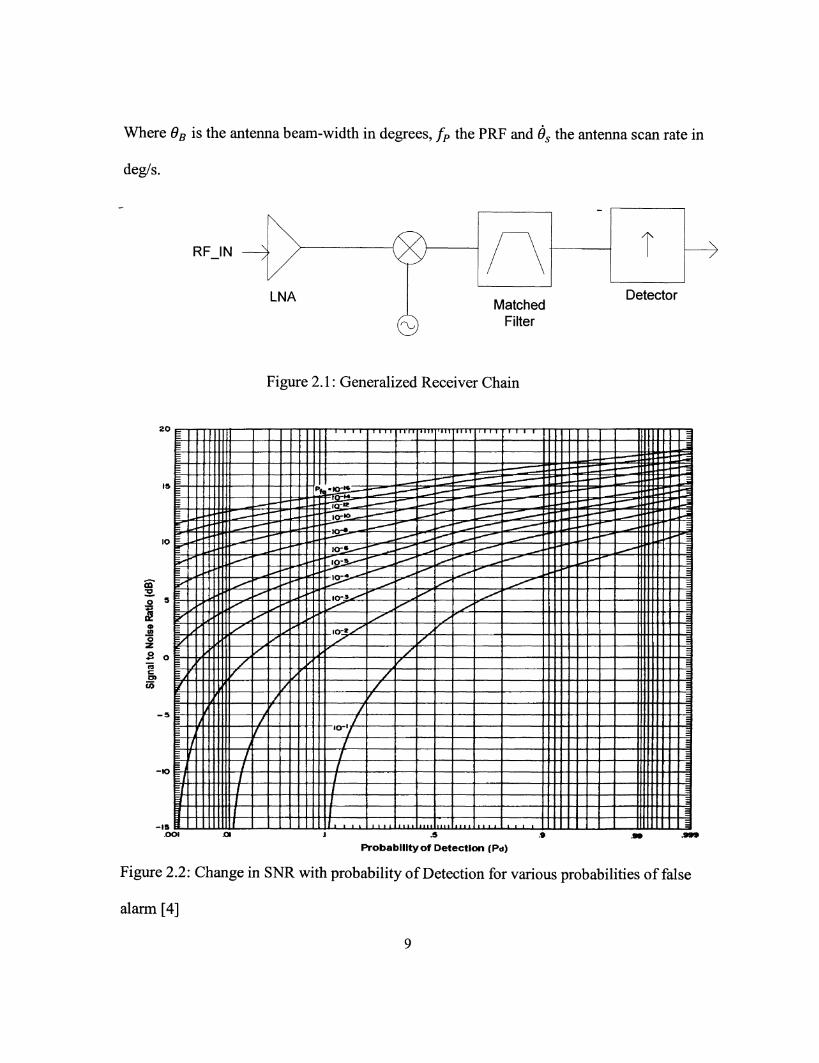
Where 9B is the antenna beam-width in degrees, fP the PRF and 9S the antenna scan rate in

deg/s.

RF IN

Matched Filter

Detector

Figure 2.1: Generalized Receiver Chain

CO

o

1

i 1 1 P 11

F 1 p f F fcs I f

& ' 1 J fc= 1JJ

E^^Pn

E "iD p^\T\ E ! IL j

r'f i p [J P ^rt i ^^ 11 J 6 >'M V P /H 12 UJ r t ts S / F J 1

§7 t ^ L i l i J r / 1 Pi 1 § ; 11 i I tjj

_J Jt

J 3

-rrr I T T T

vlaZ£E£-~^

T i b ^ ^ i +Hj^»—-* T j T JQ-* -mr

TT \jp^^-^r\C\cr^^^' JrT\\**-+. J*-

<"

T \cr*^*

i t l i o - « /

l>1 11

j | ^"lo- , /"

1 1 H i i i i

[ f I T T

i i i l

T I T T

J i l l

TTTT

m i

' J I I

I I 1

H I T

J i l l ,

; r i r r

11 i i

: 1 1 1 I I I I

^ ^ 1

_1. 1..1. 1 111

| ! 1 i = P ^

M^3 "Tl 1 ^ rU-*ri

1 [ i j =3

11 II i

i

1 1 M i M i a

1 11 | | 1 3 | ^

j j l | 1 ^

I 1 I 1 3

I 3 11

111 I I ^

J 3

1 1 [ 1

j I 3J

Probability of Detection (Pd)

Figure 2.2: Change in SNR with probability of Detection for various probabilities of false

alarm [4]

9

The filter in figure 2.1 is matched to the transmitted signal hence yielding an optimum signal

to noise ratio at its output. The detector at the filter output uses a pre-determined SNR

threshold based on the Pd and Pfa to indicate the-presence of a target. Pre-detection

integration and post-detection integration sum up the SNRs at the input and output of the

detector respectively. For pre-detection integration: SNR± = nSNRn, where SNRn is the

SNR of a single pulse while SNR± is the total SNR of the integrated pulses [5]. For post-

detection integration:

SNRi = nEi(n)SNRn, where £j(n) is the integration efficiency. Et(ri) depends on the type

of detector used and is usually experimentally determined. Equation 2.3 can be expressed in

terms of SNR± by replacing the minimum received power with equation 2.9.

Prmin = kT0BnFnSNRn (2.9)

Where Fn is the noise factor, k is Boltzmann's constant, T0 is room temperature and Bn the

noise bandwidth. Substituting equation 2.9 in 2.3 and replacing SNRn with —pr yields

equation 2.10.

n 4 _ PtG2A2<™Ej(n) .

"max ~ ^nykToBnFnSNRl VAV>

Target cross-sections are classified into five Swerling categories according to their

probability distribution function (pdf) and their pulse to pulse cross-section variation. The

pdf for Swerling I and II is given in equation 2.11 and is shown in figure 2.3 for an average

cross-section of 2m2.

10

PO) = -r-exp {-a/oave). (2.11) °ave

For Swerling I, the cross-section is constant throughout the scan but independent from scan

to scan while Swerling II has an independent cross-section from pulse to pulse. The pdf for

Swerling III and IV is shown in equation 2.12 below and is also shown in figure 2.3 for an

average cross-section of 4m2.

4<T

PO) = — exp (-2a/aave) °ave

(2.12)

Again, for Swerling III, the cross-section is constant throughout the scan but independent

from scan to scan while Swerling IV has an independent cross-section from pulse to pulse

[4]. Due to target fluctuation, additional SNR to that required for a non-fluctuating target is

required to achieve a specified probability of detection. Figure 2.4 shows the variation in

additional SNR with probability of detection for all four Swerling cases.

Swerling I and II Swerling III and IV

E 5000

0 2 4

Cross-Section Area (sq-metres) Cross-Section Area (sq-metres)

Figure 2.3: Probability distribution function for Swerling targets

11

301 r r ,m"-i 1 1 r—\—r~t—r—\ \ r™—r

- 5 i _ J L_J I I I I \ A ..,!.,. i I I I aoi ao* ai 0.2 a* ua u.f a * at* ass oss

P*©bot>ility ot detection

Figure 2.4: Plot of Additional SNR with Probability of detection for Swerling 1 - 4 [4]

2.2 Background on System Hardware

The hardware used to implement the Radar system in this thesis is designed by D-TA

Systems and it is comprised of two software radio systems and a computer. The first software

radio labeled D-TA 2300 receives a waveform in the form of packets from the computer and

converts it to an analog signal. It also digitizes analog signals and groups them into packets

in accordance with a user-specified packet size. Its DAC frequency is tunable; the maximum

DAC frequency with interpolation is 500 MHz and 130 MHz without. This puts a 62.5 MHz

limit on the signal bandwidth and 250 MHz limit on the center frequency. The maximum

ADC sampling frequency is 130 MHz and this places a 62.5MHz bandwidth restriction on

the input signal. Figures 2.5 and 2.6 show block diagrams for the D-TA 2300 and D-TA 3290 12

respectively. The D-TA 2300 stores data from the PC in a buffer (FIFO) for DAC sampling.

The DAC chip possesses a programmable interpolator and an NCO for up-conversion. The

maximum NCO frequency is half the DAC chip sampling frequency after interpolation. DAC

chip sampling is obtained from the Phase Locked Loop shown in figure 2.5. The PLL

operates off a lOOMHz TCXO reference input and a VCO with range of 375MHz to 415MHz

at its output. During transceiver operation, when both the ADC and DAC are in operation,

their sampling clock is obtained from the same VCO. This implies that even though they may

have different divider ratios, their base factor is always the same. Antenna sizes are inversely

proportional to the carrier frequency implying the higher the carrier frequency, the smaller

the antenna. To obtain a carrier frequency which yields a reasonable antenna size, a carrier

frequency of at least 1GHz is required and to achieve this carrier, an RF system is needed.

The D-TA 3290 accepts an input signal centered at 70MHz with a 40MHz bandwidth and up-

converts it to any frequency in the 0 to 6GHz range. It also accepts an RF input in the 0 to

6GHz range and down-converts to 70MHz with 40MHz of bandwidth. The input and output

IF filters are both centered at 70MHz with 40MHz of bandwidth. The D-TA 3290 utilizes 4

synthesizers in different combinations for up-conversion and down-conversion as depicted in

the UCON and DCON circuitry respectively to achieve the required RF range. Both the

UCON and DCON generate their respective outputs depending on the user-specified

(programmable) RF and IF output frequencies. The filter bank at the mixer output for DCON

and input for UCON consist of filters which select different frequency bands in the 0-6 GHz

range. Switches are placed at their inputs and outputs to select the appropriate frequency

band. A power amplifier is the final link in the up-converter chain. The down-converter has 4

13

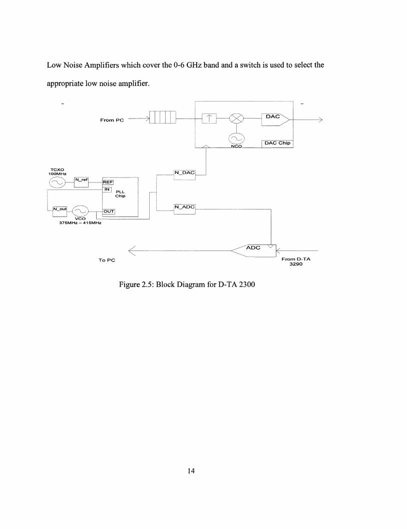
Low Noise Amplifiers which cover the 0-6 GHz band and a switch is used to select the

appropriate low noise amplifier.

From PC

T C X O lOOMHz

PLL Chip

3 7 5 M H z - 4 1 5 M H z

To PC

T

N_DAC

N ADC

D A C \

DAC Chip

A D C K-

From D-TA 3290

Figure 2.5: Block Diagram for D-TA 2300

14

">!

7 0 M H z center with

4 0 M H z bandwidth

From D-TA 2 3 0 0

R F O U T

Switch Filter Bank P A

U C O N

D C O N

T o D-TA 2 3 0 0

<~

R F _ I N

7 0 M H z center with

4 0 M H z bandwidth

Filter Bank LNAs

Figure 2.6: Block Diagram for D-TA 3290 (RF Up-converter)

2.3 Specifications

R = 1 0 k m

R G E T

(ht) 2 7 0 m

2 7 0 m

I M A G E

Figure 2.7: Radar Geometry

Figure 2.7 shows the line of sight and multipath echoes of a radar antenna with 30m of height

(hr) transmitting to a target 10km away at a height of 270m (ht). The multipath delay is

15

derived from the geometry of figure 2.7. The delay is inversely proportional to range and

directly proportional to target height. This implies that the minimum delay is obtained at the

maximum range and smallest elevation. The range (R) defines the line of sight echo while Rl

and R2 define the interfering echo. With known values of range, elevation, Rl and R2 as

depicted in figure 2.7, the expression for multipath delay can be derived as shown below.

R2 + R3 = R1 + R2= V(^t + K)2 + R2- (ht - hrY = JR2 + 4hthr

ALT1=—,AT2 = iR+Rl*R2)

c c

HA 1*.- +u J i r \ A ^ Arr R!+R2-R jR2+4hthr-R fl(l+-^J1)0"5-K r

Multipath delayir) = AT2 - A7\ = ——-— = L-z— = fi = 5.4ns

Using binomial expansion for 4hthr « R2

c R*c v f

By setting the target range in figure 2.7 to equal the unambiguous range,

PRI = 25 = 2 * -i2L = 6.67 * 10"5s = > PRF = 15kHz. C 3*108

The DTA-2300 has a maximum packet size of 4096 samples for the ADC. This implies that

the maximum PRI length that can be contained in a single packet is 65.536us, or a minimum

PRF of 15.26kHz. The corresponding unambiguous range is 9.8304km. The maximum range

for a single pulse is limited by the D-TA 3290 parameters and is calculated with equation

2.10.

16

Where Pt = WW, G = 20dB, X = 0.15m, a = lm 2 , kT0 = -174dBm/Hz, Number of

pulses - n = 1, Integration Efficiency - E^ri) = 1, Noise Bandwidth - Bn = 40M//z, Noise

Factor - Fn = 10, Single pulse SNR - (£) = 6.02dfi. Substituting the above D-TA 3290

specifications into the range equation yields a maximum range of 649.54m. The above

equation however, ignores the compression gain (Gc). Including the compression gain in the

range equation (2.10) yields the following result in equation 2.14.

R'max = P ^ A W ' % (2.14)

Gc in a phase-coded compression scheme is a function of unambiguous range.

Gr = - = 2*™*"»fr (2.15)

Where Tc is the chip width and RUnambig = 9.8304/cm from ADC packet size limitations.

Substituting for Gc in the range equation yields equation 2.16.

The optimum Tc occurs when the signal bandwidth equals the noise bandwidth. To achieve

2 2

this, Tcopt = — == — 50ns. Tc is also limited by the baseband sampling rate (Fs) which

is 62.5MHz in this case. Since Tc must be a factor of 1/Fs, The closest Tc to the optimum is

64ns. Substituting the maximum achievable chip length in addition to the other system

parameters into the range equation yields a new maximum range of 3.69km. To achieve the

required unambiguous range, either pulse integration or an increase of transmitted power is

17

required. To ensure low power utilization, pulse integration is utilized and at least 80 pulses

are required to achieve the unambiguous range.

2.4 Chapter Summary

This Chapter shows the derivation of the Radar equation. Based on the Radar equation,

curves are derived which show the relationship between the SNR, probability of false alarm

and probability of detection. It also shows the probability distribution for classification of

Swerling targets. This chapter then provides an overview of the hardware used to implement

the waveform testing. Finally, starting parameters for the waveform design are obtained from

given specifications and hardware constraints.

18

Chapter 3

Waveform Design

3.1 Phase-Coded Pulse Compression

This thesis is based on the implementation of a system with low peak output power (tens of

Watts) which achieves comparable maximum range to systems with kilo-Watts of power.

Systems with long pulse widths require less transmitter power but suffer from poor range

resolution if pulse compression is not utilized. This implies that a transmitted signal with

pulse width equal to the PRI can be optimized for minimal output power provided an

optimum pulse compression scheme is chosen. An optimum compression scheme implies

maximum gain, minimum side lobes and optimum resolution. The two most common

compression schemes are phase coded waveforms and frequency modulated waveforms.

Phase coded waveforms consist of a group of chips/bits where the chip duration is the

inverse of the IF bandwidth. Multiplying the chip sequence by the carrier waveform either

maintains the phase of the carrier pulses per bit duration or flips the phase by 180 degrees.

The received signal delay is obtained by varying the transmitted signal delay, and at each

delay the received sequence is multiplied and added with its corresponding transmitted

sequence. This process is called auto-correlation. Cross-correlation is realized when the

received signal is multiplied and added to a different transmitted sequence. Maximal-length

sequences (MLS) have a correlation peak value equal to the number of chips and a value of

-1 at every other delay. These sequences are derived from primitive polynomials and have

19

randomness characteristics similar to those ascribed to truly random sequences. Any

polynomial can be implemented in hardware with shift registers and an X-OR gate. The

number of shift register stages (n) determine the length of the sequence and highest degree of

the polynomial while the inputs to each X-OR gate determine the type of polynomial. If the

generated polynomial is primitive, a maximal-length sequence is obtained with a length of

N = 2n — 1 before repetition. Given n shift register stages, the total number of maximal

length sequences is given by equation 3.0.

Af = Jn(l-^) (3-0) rl Pi

Where pt represents the prime factors of N [20]. Since a maximal length sequence is

repetitive after N chips, PRIs with pulse widths equal to NTchip achieve pulse compression

but still suffer from range ambiguity. Range ambiguity can be resolved by transmitting a

different sequence every PRI. In this way, unambiguous targets are processed using the auto

correlation function while ambiguous targets are processed using cross-correlation. A

transmission scheme implemented in this manner with a different MLS per PRI is hardware

intensive because M primitive polynomials for a specific number of shift registers (n) have to

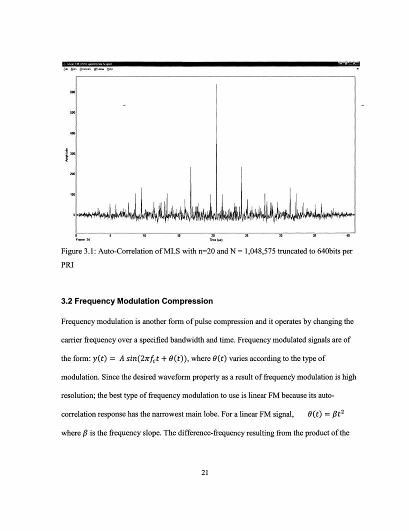
be found and a different polynomial implemented per PRI. An alternative to this is using

truncated portions of a single MLS for each PRI with the drawback being higher side-lobe

levels for certain sequences as shown in figure 3.1.

20

£ile &xes £hanneb itfndow Help

liraelpsjj

Figure 3.1: Auto-Correlation of MLS with n=20 and N = 1,048,575 truncated to 640bits per

PRI

3.2 Frequency Modulation Compression

Frequency modulation is another form of pulse compression and it operates by changing the

carrier frequency over a specified bandwidth and time. Frequency modulated signals are of

the form: y(t) = A sin(2nfct + 0(t)) , where 9{t) varies according to the type of

modulation. Since the desired waveform property as a result of frequency modulation is high

resolution; the best type of frequency modulation to use is linear FM because its auto

correlation response has the narrowest main lobe. For a linear FM signal, 9(t) = /?t2

where /? is the frequency slope. The difference-frequency resulting from the product of the

21

sent and received signals has a constant frequency offset (Af) which depends on the target

range [7]. If Af is known, target delay (Tr) can be obtained from equation 3.1.

?V = £ " = T " (3-D

Where T is the chirp period, AF is the difference between the maximum and minimum

frequency, R the range and c the speed of light. This implies that theoretically, frequency

modulated waveforms can have no resolution limit. However, in digital systems, the smallest

observable delay and hence resolution limit is the inverse sampling frequency. For digital

reception and processing, range and Doppler from linear FM pulses can be obtained by

correlation and filtering respectively in that order. The processing is identical to that for

phase-coded waveforms except that phase-codes use linear correlation while linear FM uses

circular correlation. Analytical derivation of the linear FM auto-correlation function is shown

below.

ychirp = e^w n +^n \ w is the starting angular frequency, /? the angular frequency slope and n

the discrete time.

Ac(n) = £/c=-oo e^wk+^k^e^k+n^+^k+n)2\ where Ac(n) represents circular auto

correlation. From Z transform properties,

If/i(n) = eJ(wn+^n2)

ThenAF(0 = H(0-(H(Oy

Where AF(f) = F{Ac(n)} &/ / ( / ) = F{h(n)}

22

I 7T/2

/ / ( / ) = |^~- e JP from Fourier transform properties implying

AF(f)= —e JP * — e JP =-

=> Ac(xO = F-HAptf)} = J*(n). (3.2)

Note that the above Fourier transforms are valid for an infinite time domain signal. From the

above derivation, it can be observed that the auto-correlation of an infinite time and

continuous linear chirp yields a delta function scaled by a constant. For practical purposes, an

infinite time domain signal is unachievable and as a result, the auto-correlation deviates from

the ideal delta function by introducing side-lobes and degrading peak resolution. The non

idealities can be observed in figure 3.2 which is the auto-correlation response of a linear

chirp ranging from 0 to 15.625MHz with a 62.5MHz sampling frequency (16ns sampling

period). Based on the range and sampling frequency, /? = 2 * pi * '• — =

S.998E12rad -,N = 1023. 1023 values of h(n) are obtained from 0s-1023*1.6E-8s. The auto-

correlation shown in figure 3.2 is obtained by finding the Fourier transform of h(n),

multiplying by its conjugate and taking the inverse Fourier transform.

23

-5 0 5 Delay (x1.6e-8s)

Figure 3.2: Auto-Correlation of linear-FM chirp

It can also be observed from the auto-correlation function derivation that the starting

frequency for the chirp given by 'w' does not affect the auto-correlation response hence the

transmitted signal can be simplified to h(n) = e ^ n ' .

3.3 Phase-Coded-Linear-FM

Linear FM pulses have superior resolution over phase-coded compression because the chip

width limitation of the phase coded waveform is IF bandwidth whereas a frequency

modulated waveform can change at the sampling frequency. Since the processing of both

24

linear FM and phase-coded waveforms is similar, a compression scheme can be designed

which exploits the advantages of both waveforms. Convolving a triangular FM pulse with a

random pulse train yields such a compression scheme. Convolution ensures that the delta

function auto-correlation responses of both the phase-codes and linear chirps are maintained

in the combined waveform. The random pulse train ensures that returns outside the

transmitted pulse train are cross-correlated and this brings about rejection of ambiguous

targets. The derived waveform benefits from improved resolution as target resolution is

determined by the triangular FM pulse. It also benefits from a lack of range ambiguity as a

result of phase coding because random pulse correlation ensures that second time around

(and higher) targets are rejected. In order to reject ambiguous targets, echo processing should

be a cross-correlation as opposed to auto-correlation for unambiguous targets. Since the

linear FM signal is repetitive every PRI, its cross-correlation is equivalent to its auto

correlation. Phase codes on the other hand have separate auto-correlation and cross-

correlation properties. The combination of phase codes and linear FM properties in a single

waveform should be done in such a way that the delta function auto-correlation property is

preserved. Preservation of the delta function auto-correlation property is done by convolution

of a phase-coded waveform with a linear FM waveform and analytical proof is shown below.

h(n) = e^n2)®ei(0(n))

= > AP(f) = F{e^n2)®eK* (n))} * F{e~^n2>>®e<e^} = - * N

25

A convolution in time domain is equivalent to a multiplication in the frequency domain thus

the above expression reduces to the multiplication of the Fourier transform of each of the

individual componentSr The linear FM products reduce to - while the phase coded products

reduce to the number of chips (N).

=>Ac(n)=^*N*S(ri) (2.3)

From the auto-correlation expression above, we can notice that the correlation gain of the

chirp has been multiplied by the correlation gain of the phase coded waveform. Figure 3.3

shows the auto-correlation response of the convolution of the linear FM waveform with a

1023 chip maximal length sequence. Since the phase modulated signal is a MLS, the

convolved waveform shown in figure 3.3 is a approximately equivalent to the product of the

response shown in figure 3.2 and a discrete ideal delta function. The correlation gain can be

observed to be 1.046E6 as determined by the product of the chirp gain (1023) and the

number of MLS chips (1023). In reality, the extra factor of N in the correlation gain of the

phase-coded-linear-FM signal is not achievable for a fixed output power level because the

power of the convolved waveform is the sum of the chirp power and phase coded waveform

power in dB. The auto-correlation expression above also shows us that the applying a phase

coded waveform to the chirp does not affect its correlation response thus the radar system

can benefit from the high resolution of a chirp compared to a phase-coded waveform for a

fixed bandwidth. The cross correlation derivation of the phase-coded-linear-FM waveform is

shown below.

26

Xc(n) = (ej^n2)®eJ(0(n)))(g)(e-K^"2)®e-j(a(n))). From the associative convolution

property, this can be rearranged to:

= > Xc(n) = 2(eJ(»Cn))0e-j(a(n))) (3.4)

Where a(ri) and 9(ri) are two different PN sequences. Optimally, the cross-correlation

should be 0 but PN sequences have poor cross-correlation properties with cross-correlation

values of up to 0.35*N for certain sequences [8]. Due to the relatively small number of

maximal length sequences for a given N, partial sequences have to be used for correlation.

Delay (x1 6e-8s)

Figure 3.3: Auto-Correlation of convolved phase modulated and linear-FM signal

27

The drawback to using partial length sequences (PLS) is their auto-correlation response

approximates the delta function. The auto-correlation gain of a PLS is equal to the length of

the sequence as in a MLS but the PLS. contains side-lobes as opposed to no side-lobes from a

1 1 1 MLS [91. Given the following base-bandwidth restriction:/? = — = — = =

L J & Tc 4TS 4*1.6E-8

15.625M//Z, and PRI restriction of 65.55us, the chirp gain (B*PRI) is 1024 and the number

of phase-code chips is 1024. Figure 3.4 shows the cross-correlation or second time around

target rejection over multiple partial sequences of the transmitted waveform. The transmitted

waveform is obtained by the circular convolution of a chirp with bandwidth-time product of

1024 and a truncated PN sequence consisting of 1024 chips from a 20-bit LFSR. It can be

observed that the attenuation factor ranges from 0 to 0.25 with an average of 0.15.

Figure 3.4: Normalized peak cross-correlation value over successive pulses

28

3.4 Chapter Summary

This chapter examines the properties of both phase and frequency modulated waveforms and

derives their individual auto-correlation responses. It then uses their individual-correlation

responses to derive the auto-correlation response of the phase-coded-linear-FM signal.

Finally, this chapter looks at the cross-correlation properties of the phase-coded-linear-FM

signal.

29

Chapter 4

Radar Simulation in Matlab

4.1 Transmitter

This chapter generates and simulates a model in Simulink to verify the ability of the

proposed waveform to reject noise and jamming, accurately detect targets in the presence of

multipath, and detect range and Doppler in the presence of noise.

As derived from the radar specifications, a chip rate (inverse of chip length - Tc) of

15.625MHz at a 62.5MHz sampling rate is required to achieve maximum compression gain.

The PRI is determined in the specifications to be 65.536us. The phase-coded-linear-FM

cAt waveform also compresses the pulse to achieve finer resolution given by R = — =

0170^1 tip O : = 2.4m, where At is the inverse of the sampling frequency. Figure 4.1 shows the

Simulink block diagram used to implement the phase-coded-linear-FM waveform. The

phase-codes or chips are obtained from a 20 bit LFSR and converted to a bipolar from a

PRI

unipolar format. The number of chips per PRI is obtained as follows: N = — =1024.

These chips are convolved with a triangular FM pulse ranging from DC to 15.625MHz and

lasting 65.536us. Note that the FM compression gain given by its bandwidth-time product is

equal to the number of phase coding chips. Figures 4.2 and 4.3 show the spectra of both chirp

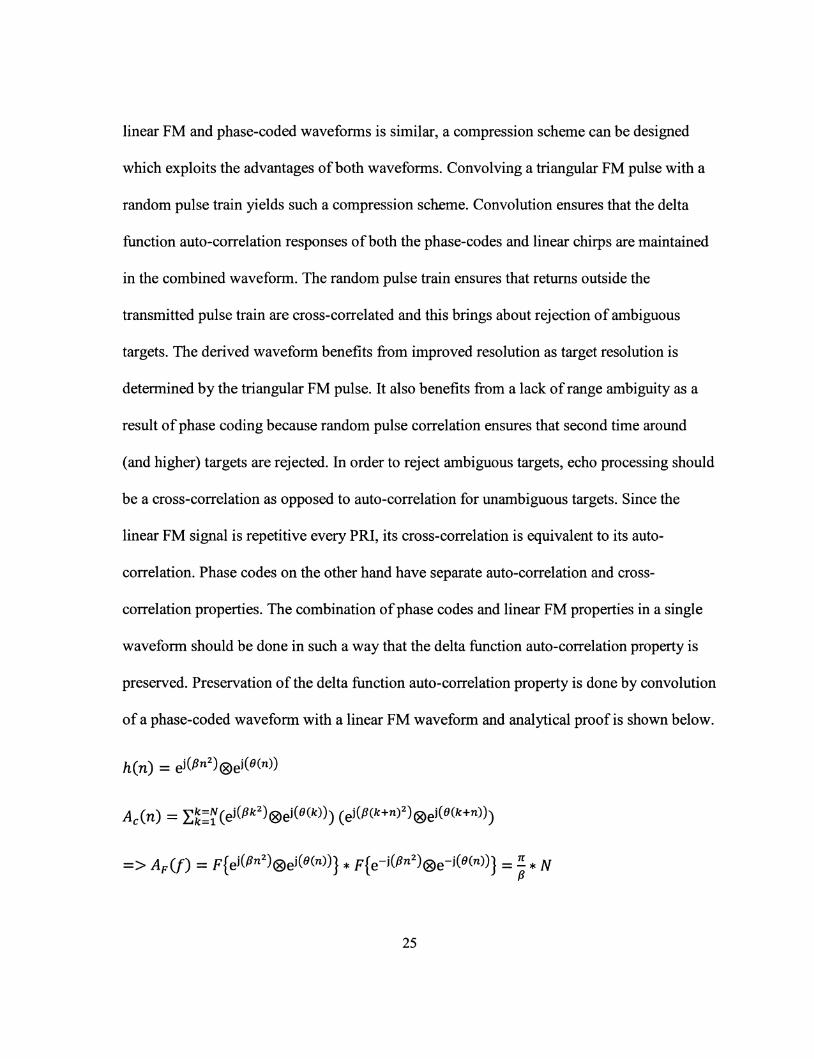
and phase modulated waveforms respectively; the product of one spectrum with the

30

conjugate of the other yields the spectrum of the phase-coded-linear-FM waveform in figure

4.4.

A/W I Chirp

PN Sequence Generator


Unipolar to Bipolar &H H

DSP Constant

FFT

X

Productl

IFFT

IFFT I

I Out2

Figure 4.1: Block Diagram for the transmitter

.^rompM^ Rle View Axes Channels Window Help

j $ JS> J2> x

-80

-100

-120

-140

-180

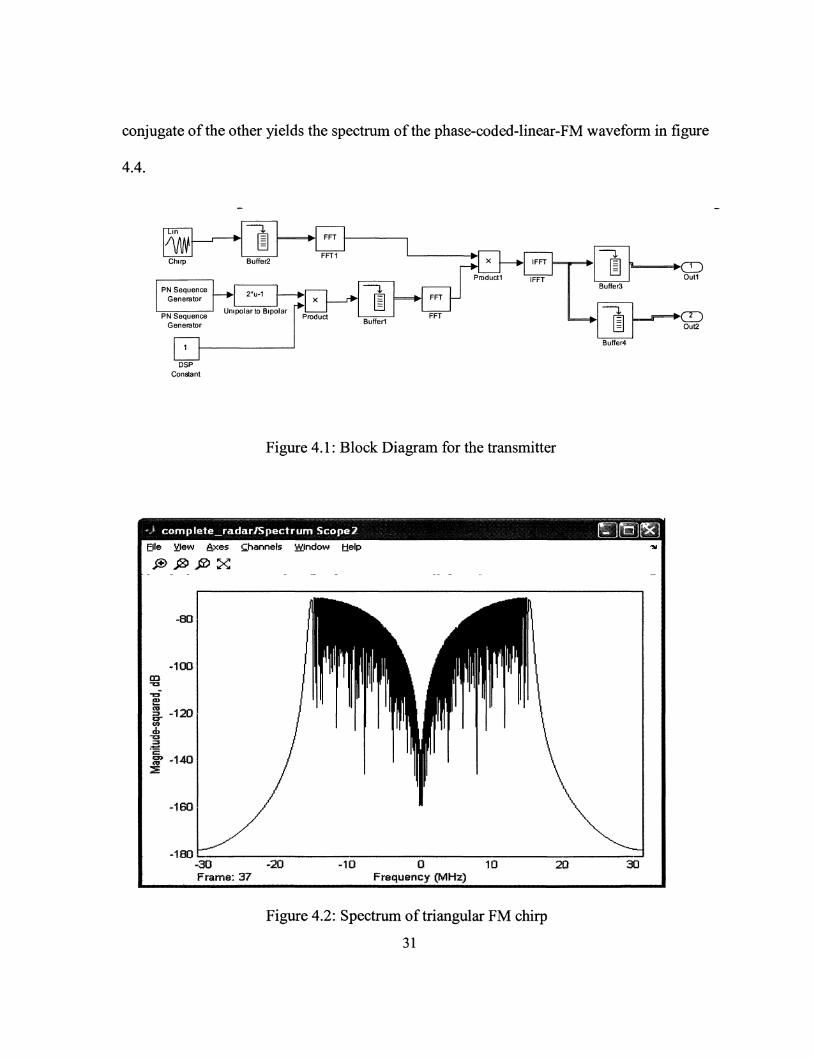
-180 -30 -20 Frame: 37

-10 0 10 Frequency (MHz)

Figure 4.2: Spectrum of triangular FM chirp

31

B a untrtted/Spectrom Scope

£»te View A M S Channels Winda* Help

^^LM

Frequency |MHi}

Figure 4.3: Spectrum of phase modulated signal

Filt A*es Chsnntli Window Help

F w j i i * s e y i M « #

Figure 4.4: Spectrum of phase-coded-linear-frequency-modulated signal

32

The spectrum shown in figure 4.2 is that of a triangular FM signal and it is different from the

spectrum of a linear FM signal which is approximately flat. The equal but opposite frequency

slopes of the triangular FM signal cause the resulting null at DC. The phase modulated signal

is pseudo-random noise hence its approximately flat spectrum as shown in figure 4.3.

4.2 Channel

The channel effects considered in this model are multipath, noise, target cross-section and

Doppler shift. As shown in the Specification section, multipath delay depends on the range

and elevation of a particular target. Individual multipath components cannot be separated

unless the multipath delay is greater than the time equivalent of the target resolution as

determined by the transmitted waveform. In this case, target resolution is determined by the

inverse of the sampling frequency - 16ns. For range measurements, the ability of the receiver

to separate multipath components does not affect range accuracy as long as the path with

minimum delay is chosen. As a result degradation in accuracy due to multipath only occurs

when determining target elevation. Multipath is modeled by adding a delayed version of the

transmitted signal to the transmitted signal. Since the LOS and delayed paths are different,

their respective free space losses and antenna gains are computed before addition. Additive

White Gaussian noise is generated by an existing Simulink block and added to the

transmitted signal with a signal to noise ratio at the receiver of lOdB including processing

gain and -20dB without processing gain. Free space path loss is computed by the expression

in equation 4.0.

33

A2

(4TT) 2 R 4 I = 7 7 ^ " (4-0)

Implying an amplitude attenuation of VT. Target Doppler is modeled by applying a

frequency shift to the carrier given by equation 4.1

fd=f (4-D Where v is target velocity, fc is the carrier frequency and c the speed of light. The target

constitutes part of the channel and is implemented as a delay in echo reception. Moving

targets have variable delays in accordance to their velocities. Clutter also constitutes part of

the radar channel and it comprises of stationery and sea clutter. Stationery clutter results from

non-moving targets; as a result their echoes have low Doppler shifts though not quite zero as

a result of antenna rotation. The sea comprises of waves which are due to the earth's rotation

and wind velocity, as a result echoes returning from sea waves have a non-zero Doppler shift.

Empirical data suggests that the clutter spectrum has a Gaussian shape with an additional

peak at the edge of the spectrum due to the main beam of the antenna [10]. Only the main

beam clutter frequency as determined by the sea state and wind velocity is implemented in

this model. The virtual sea clutter velocity at the peak of the clutter spectrum for X and C

band radar looking upwind at low grazing angles can be estimated by equation 4.2.

Vvir « 0.25 + 0.13U (4.2)

Where U is the wind speed [11]. Wind speeds vary from Om/s for calm seas to 36.9m/s for

hurricanes [12]. This implies that virtual clutter velocities range from approximately 0.25m/s

to 5.047m/s under various sea conditions. The resulting Doppler frequencies are 3.3Hz to

67.3Hz at a carrier frequency of 4GHz. The Simulink Channel model is shown in figure 4.5.

34

Clutter returns (as shown in figure 4.5 as delays 15-18) are positioned before the target range

bin (delay 21 in figure 4.5) to ensure the receiver's ability to detect a target in the presence of

clutter. The delay number represents the distance from the target to the Radar. The magnitude

of the auto-correlation response depends on the target cross-section and the transmitted

phase-code sequence. Clutter positioning in figure 4.5 can also be used to verify the

receiver's ability to distinguish the target from delayed (multipath) components of the

transmitted signal. More multipath components can be used in figure 4.5 but the purpose of

this test is to verify the receiver's ability to distinguish components separated by more than

one delay unit.

AWGN Channell

C D \—•

AWGN Channel

3F ~ =1 AWGN

AWGN Channel3

AWGN Channel4

Phase/ Frequency

Phase/ Frequency

Offset4

Phase/— Frequency

Offset

Phase/ Frequency

Offset

Phase/ Frequency

Offset

Phase/ Frequency

Offsetl

AWGN Phase/

Frequency

Phase/ Frequency

Offset2

Free Space Path Loss

75 dB

Free Space Path Loss2

\


75 dB Phase/

Frequency Offeet3

Phase/ Frequency

Offset

^

Delayl

-21 z

Free Space Path Lossl

Delay


76 dB

DSP Constantl


MATLAB Function


74 dB


Delay4


74 dB


tu. roduct2 itjr

CD Out1

Figure 4.5: Block Diagram for Radar Channel

4.3 Receiver Processing

The receiver is implemented by buffering the received bits per PRI and correlating the entire

PRI with the transmitted sequence. The correlation processing gain (pulse width/chip length)

35

due to the phase coded effect of the waveform is lOlog (N) = lOlog (1024) = 30.1dB since

1024 chips are sent per pulse [13]. The correlation processing gain due to the frequency

modulation property of the waveform is the bandwidth-time product: lOlog (BT) = lOlog

(15.625M*65.536u) = 30.1dB. The total processing gain is the sum in dB of the individual

processing gain yielding a total gain of 60.2dB used to improve the receiver SNR hence the

probability of detection. Since the transmitted waveform is continuous, each received PRI

contains both the current and previous transmitted sequence. As a result, correlation is

implemented by taking the FFT of the received sequence and the last two transmitted

sequences. The received PRI spectrum is multiplied by the complex conjugate of the

transmitted sequence spectrum before taking an inverse FFT to yield the time domain auto

correlation response. It is advantageous to use FFTs for correlation of long sequences

because the processing time is 3N * logN + N compared to N2for a traditional correlation

algorithm where N is the number of samples per PRI [14]. The receiver block diagram in

figure 4.6 shows the correlation processing. Depending on the target cross-section, the auto

correlation value for the target range bin varies. Figure 4.7 shows the auto-correlation

response for the Swerling III and IV pdf while figure 4.8 shows the auto-correlation response

for the Swerling I and II pdf. The target range bin is the second peak in both figures 4.7 and

4.8 which appears at 32.94us. Due to the nature of the Swerling I and II pdf, the cross-section

returns are much higher compared to Swerling III and IV as can be observed from target

auto-correlation values shown in figure 4.7 and 4.8. The receiver can also distinguish returns

separated by at least 16ns as shown in figure 4.7 and 4.8 thus verifying the receiver's ability

to distinguish LOS from multipath components. Also, since the delay between the clutter and

36

target peaks as shown in figure 4.8 and 4.9 is 48ns. The waveform range resolution is also

verified for targets separated by 3 range resolution bins. The maximum peak corresponds to a

clutter return with a virtual Doppler frequency of 67Hz while the second most prominent

peak corresponds to a target moving a velocity of 300m/s.

C D - * In1

Pad

Pad

In2

FFT

FFT

FFT

FFT1

^ W

u _ i

Complex Conjugate

^ w -^

X fe.

Product

IFFT

IFFT

• C D Out1

Figure 4.6: Block Diagram for Receiver Correlation Processing

1 ~*J>> f i n a l r a d a r nr iodei /Vect :or^:Si : i>0i fe : i l l l iS^ i i '

IOOGO

9000

8000

7000

sooa

M_ 50QO

*• 4GOO

3000

2C3GHDt

1000

O

&xes Channels Window fcielp

js» x:

32.6 32.7 32.8 F r a m e : 1 5

^•iWiii iWWlf

32.3 Tim© ( j*s)

BB 1 *

33

*v ^ > ^ ' •-/£ . A, ,

33.1

^ l o l *tl *m j

33.2

Figure 4.7: Simulated Auto-Correlation Response for a Swerling III or IV target

37

•iji.uBii.i.uji..i.i.umjjjj.imj.i ©I© View Axes Channels Window £tel&

,rr,lPt2Sl

,£> JS» J2> JXI

32.82 32.84 32.88 32.88 Frame: 112

32.9 32.92 32.94 32.96 32J Time (M-S)

Figure 4.8: Simulated Auto-Correlation Response for a Swerling I or II targets

The Doppler frequency is obtained by computing the FFT of the complex auto-correlation

result over successive pulses. Computing the Doppler shift in this way is called Serial

Doppler processing. Since the waveform is a Spread Spectrum, the carrier is masked thus

correlation should be used to extract the return from the noise floor before processing. Figure

4.9 shows the spectrum of auto-correlation values sampled at the PRF for the target range bin

obtained from figure 4.8. The auto-correlation values are stored over 256 pulses for a target

moving at 300m/s and a signal with carrier frequency of 4GHz. The required Doppler

frequency given the above specifications is 4kHz (from fd = —-£ and the frequency which

provides the peak magnitude obtained from a 256 point FFT is observed from figure 4.9 to

4.12 to coincide with this value. Figure 4.9 shows the Doppler frequency at the target range

38

bin for a Swerling I target. Frequency shifts due to the target and clutter are observable at this

range bin because the target cross-section is much smaller than the clutter cross-section. For

a Swerling II target, the target Doppler shift is again observed at the expected frequency (as

shown in figure 4.11) although, the carrier to noise ratio is less than that for Swerling I

targets because of the pulse to pulse variation in cross-section. Swerling III has a high carrier

to noise ratio (as shown in figure 4.10) like Swerling I but without the clutter Doppler shift

because the Swerling III cross-section is much higher that the clutter cross-section. The

carrier to noise ratio for a Swerling IV target is smaller than that of Swerling III as observed

in figure 4.12 due to pulse to pulse cross-section variation. Its carrier to noise ratio is also

greater than that of Swerling II due to its higher cross-section return and no dominant peak is

observed at the clutter Doppler frequency for the same reason. The Doppler frequency at the

clutter range bin is shown in figure 4.13 and it shows a peak frequency at 67Hz. The received

clutter has a high carrier to noise ratio as clutter is simulated with a non-fluctuating cross-

section.

39

Uj f inal r adar m o d e l / S p e c File View Axes Channels

| JS> JS> J2> X

85

80

75

en 70

1 | 65

w* 60 a>

1 55 as

25 50

45

40

35

C } 1 Frame: 2

€ r u * i i i £ M i ^ ^ Window Help

2 3 4 Frequency (kHz)

£ i > / v v <, v

5 6

.^Jmi *< * M

7

Figure 4.9: Doppler Spectrum for Swerling I target

1 ~jfc final radar model/Spe£b^m:'# File View Axes Channels Window Help

•M?> V * - »-;- ., ^ l o l x | *S* :

| j£> J » J2> X

100

95

90

<g 85

| ao

d» 75

H> 70

65

60

55

50 C J 1 2 3 4 Frame; 2 Frequency (kHz)

5 6 7

Figure 4.10: Doppler Spectrum for Swerling III target

40

• * 1. fir^l . ^ H ^ r rvtrtrf <*i / ^ p ^ ^ ^ ^ t t * ^ ' ^^^pPIIiiiillllllH^^^^^

Epe Jfiew ftxes Channels SSJJndow Help

X j

•*»

( «£> J2> JS> X

S3

m 7°

jaw <**

B* SO

-^

I s SO

40

3G

/ \

V'| wifK n / v | p

0 1 2 3 4 5 8 7 Fr&mG: 2 Frequency (kHa)

Figure 4.11: Doppler Spectrum for Swerling II target

.> final radar model/ File ^ e w Axes Channels Window Help

'"fm,*, ^ l Q l 2 d

js> JS J2> X

0 1 Fr&me: 2

3 4 Frequency (kHz)

Figure 4.12: Doppler Spectrum for Swerling IV target

41

Virtual clutter velocities as obtained from equation 4.2 range from approximately 0.25m/s to

5.047m/s under various sea conditions with resulting Doppler frequencies of 3.3Hz to 67.3Hz

at a carrier frequency of 4GHz. Figure 4.13 shows the spectrum of auto-correlation values

sampled at the PRF for the clutter range bin obtained from figure 4.8. The clutter Doppler is

67.47Hz as obtained from the sea state and figure 4.13 shows a peak power at this value. The

Doppler frequency is computed by taking a 256 point FFT at each range bin and the Doppler

shift is the frequency with the highest carrier to noise ratio.

|*jfc final_radar_model/5pect:rM;nfi :S^ 0ie £iew &*&$ Channels tt£ir

| JS> J8> J0 X

90

80

8 70

Mag

nitud

e-sq

uare

d,

o

o

40

30

20 I 0

idov* yelp

\

ukM\i\A IWl/lP' yv f

1 1 2 3 4 Fmme: 2 Frequency {kHz)

&W5. '. *lPl

\M /WV 1 if i

I

5 6 7

X | | *a*

Figure 4.13: Doppler Spectrum obtained from 1024 point FFT at clutter range bin

Processing auto-correlation values to obtain the Doppler frequency improves the signal to

noise ratio of the Doppler spectrum as we are processing on signals which have been

42

extracted from noise. From auto-correlation values, range bins with targets or clutter are

known and are used to select relevant Doppler information. Clutter can thus be rejected by

setting a threshold for the minimum Doppler frequency expected and eliminating all range

correlations returns below this threshold.

4.4 Simulated Serial Vs Parallel Processing

The determining factors for a choice between serial and parallel Doppler processing are

Doppler SNR and processing speed. Parallel Radar processing implies the range and Doppler

processing are done simultaneously while serial Radar processing implies range and Doppler

information are extracted sequentially. Range information is obtained by correlation thus in a

serial Radar process, the echo is correlated before being processed for Doppler information.

Parallel Doppler processing is easily implemented in Radar Systems with waveforms which

are repetitive per PRI. For such Radar Systems, the phase of the echo at each range bin is

exclusively dependent on the target Doppler shift. Other Radar Systems like the one

introduced in this thesis transmit different waveforms per PRI and as a result, the change in

phase at each range bin is as a result of both the target Doppler shift and transmitted

waveform properties. The detection of Doppler shift for such a system requires the removal

of the random waveform effect before Doppler processing is carried out. The waveform

proposed in this research has both frequency and phase modulated properties. The frequency

modulated property is periodic and can be viewed over successive pulses without corrupting

Doppler information. The phase modulated property, however, changes with each PRI

implying the random nature of the phase codes has to be removed such that the target

Doppler shift can be extracted. Correlation is one method of removing the random nature of

43

the echoes as the auto-correlation output is consistent at the target range bin regardless of the

transmitted phase code. Other random cancellation schemes require the detection of the

presence of a signal and the required detection scheme should take considerably less time

than it takes to correlate a signal otherwise parallel processing becomes counter-productive.

Another method of removing the random nature of successive pulses is realized by taking the

product of the transmitted and received waveforms at the appropriate delay (range bin). This

research does not examine signal detection schemes required for parallel processing. It

assumes that the radar system is able to implement signal detection with almost no delay and

it examines the difference in carrier to noise ratio at the Doppler frequency between parallel

and serial Radar processes. The time required for processing of a fast FFT is given by

NlogN, where N is the length of the FFT. Ignoring time required for multiplication,

correlation requires a processing time of 3NlogN as the FFT of the transmitted and received

sequences are computed as well as the inverse FFT of the complex product of said sequences.

To maintain the same amount of processing time between the parallel and serial processes,

the Doppler FFT length of the parallel process is chosen to be AN while the Doppler FFT

length of the serial process is N where N = 4096. Figure 4.14 and 4.15 show the carrier to

noise ratio at a known target delay and Doppler frequency of 100Hz for serial and parallel

Radar systems respectively. The simulated target is also non-fluctuating.

44

BO #mat_radar_mode!/Spectrum Scopel

File View A*es Channels Wmdow Help

j C3 j I lill'MMIflll 'V'4iWWW(lf I 1

1*

Figure 4.14: Doppler Spectrum of Serial process for non-fluctuating target

1 r"~"% \ j"*7.l l^iasaaflSM^T^^^siM final_radlar_mQdet/Spectrum Scope2

File View Axes Channels Window Help

%o ~es

e 9 «ar m

St £ = « 3 >

M

-20

-25

-30

-3S

-40

-46

-50

~S6

~€0

~6S *0.S ~0«4 -0*3 -0..2 Fr&ma: 2

-0„1 0 0 1 Fmqu&ncyr (kHar)

0«2 0 3 0„4 OS

Figure 4.15: Doppler Spectrum of Parallel process for non-fluctuating target

45

It can be observed from figure 4.14 that the Carrier to Noise ratio at the Doppler frequency is

about 55dB for the serial process while the parallel process in figure 4.15 shows a Carrier to

Noise ratio of about 28dB. The simulated improvement factor for the serial Vs parallel

process for the same processing time is 27dB.

4.5 Chapter Summary

This chapter verifies the ability of the waveform and receiver processing to detect the

presence of a target in the presence of AWGN, clutter, multipath and target cross-section

through Matlab/Simulink simulations. This chapter also verifies waveform range resolution

by observing the delay between successive auto-correlation peaks. Finally, both serial and

parallel Doppler processing is simulated in this Chapter and serial processing is observed to

have about 27dB improvement in CNR over parallel processing.

46

Chapter 5

Implementation and Testing

5.1 Real Time Processing

Tests carried out in this thesis are done to verify the improvement in the power requirement

for systems that utilize pulse compression over systems that do not. The tests also verify

target range resolution improvement of the proposed phase-coded-linear-FM waveform over

phase-coded and linear-FM waveforms. Finally, the tests verify moving target detection from

Doppler information and the improvement in CNR of a serial over a parallel Doppler

processor. Baseband processing is implemented on a PC and the block diagram is shown in

figure 5.1 below. The transmitted waveform generated by the convolution of a random PN

sequence and a linear chirp is stored in the PC's memory before being sent to the D-TA

2300. On the receive side, FFTs on both the received and transmitted sequences are done to

implement the auto-correlation function. The magnitude of the auto-correlation response is

used to display target range. The received auto-correlation responses are stored in a buffer

and FFT processing over successive pulses at each range bin is used to display the Doppler

information. Modifications to the kernel layer of the PC were required to ensure real time

processing. This important because any delay in the packet sequence of the received signal

will change the range processing from auto-correlation to cross-correlation.

47

1 >' ,

; > /

/ - ;' L in

%- fibftp'

^ - . ' V' V"" ' ' '- ' - ' ' ' '


, mmqmm" , *> s' ^

w i -<,'

CONV

1 .' I'|

To_D-TA_2300

- V < ' : ; ; ^ '

: ' s- ' N % ' ,

Fr_D-TA_2300

"';,^5»M*?WRI

! - * *-£ ";v'v

\ K ' . " ' " / X

' "' '" "-'

fr] FFT

m

FFT

- «*?* ,

~HI

&

W , '"' 1 s

'

Hfipittt&ttiitip

F

yvi

*»»*«<* , i

, * V 5„s ? A ',„

' ^ U'tfjr*-**.**

IFFT

, v l K W ( / ,

) •:-";:. •;

—*. ' r *: '*^-' —' ' %$> " \Vs;3^' ' ; - ' ^

'* ; \ - -' - *;5 ~ ..." * , " ' W ' $-;it>,y~\^

1 ' 8«8w*

'$ k

*V^,>' / '

3

H T.me

j Mill,

1 FFT

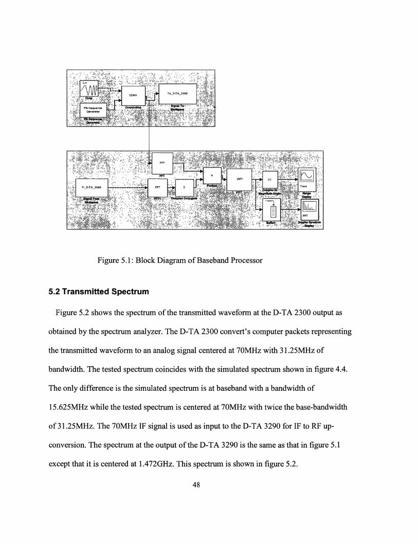
Figure 5.1: Block Diagram of Baseband Processor

5.2 Transmitted Spectrum

Figure 5.2 shows the spectrum of the transmitted waveform at the D-TA 2300 output as

obtained by the spectrum analyzer. The D-TA 2300 convert's computer packets representing

the transmitted waveform to an analog signal centered at 70MHz with 31.25MHz of

bandwidth. The tested spectrum coincides with the simulated spectrum shown in figure 4.4.

The only difference is the simulated spectrum is at baseband with a bandwidth of

15.625MHz while the tested spectrum is centered at 70MHz with twice the base-bandwidth

of 31.25MHz. The 70MHz IF signal is used as input to the D-TA 3290 for IF to RF up-

conversion. The spectrum at the output of the D-TA 3290 is the same as that in figure 5.1

except that it is centered at 1.472GHz. This spectrum is shown in figure 5.2.

48

hp REF 0 . 0 d B n ftTTEN 1 0 dB

CENTER 78.0 MHz RES BM 308 kHz

MKR 71.33 MHz -20.50 dBM

'J1

f in

JaJf idl

^>*m

j

fyjjJ F| n V

J * l M r » «

/

* M ^

\ ,

\

Vlu*«.

"" w ^ \ "

\ >,

UBM 1 MHz SPAN 82.9 MHz SMP 20.0 Msec

Figure 5.2: Output of D-TA 2210 as seen on Spectrum Analyzer

faj-j R E F 0 . 0 d B n

1 0 d B /

A T T E N 1 0 dB MKR 1 . 4 7 0 5 6 GHz

- 2 . 1 0 d B n

w f) v

ftr ^

, lA*

y v ^ - ^ fW-Av -V^

\

\

\ 1

^ • i * . s \

In *«Mkw

C E N T E R 1 . 4 7 2 0 GHz RES BM 3 0 0 k H z UBM 1 MHz

SPAN 80.0 MHz SMP 20.0 nsec

Figure 5.3: Output of D-TA 3290 as seen on Spectrum Analyzer

49

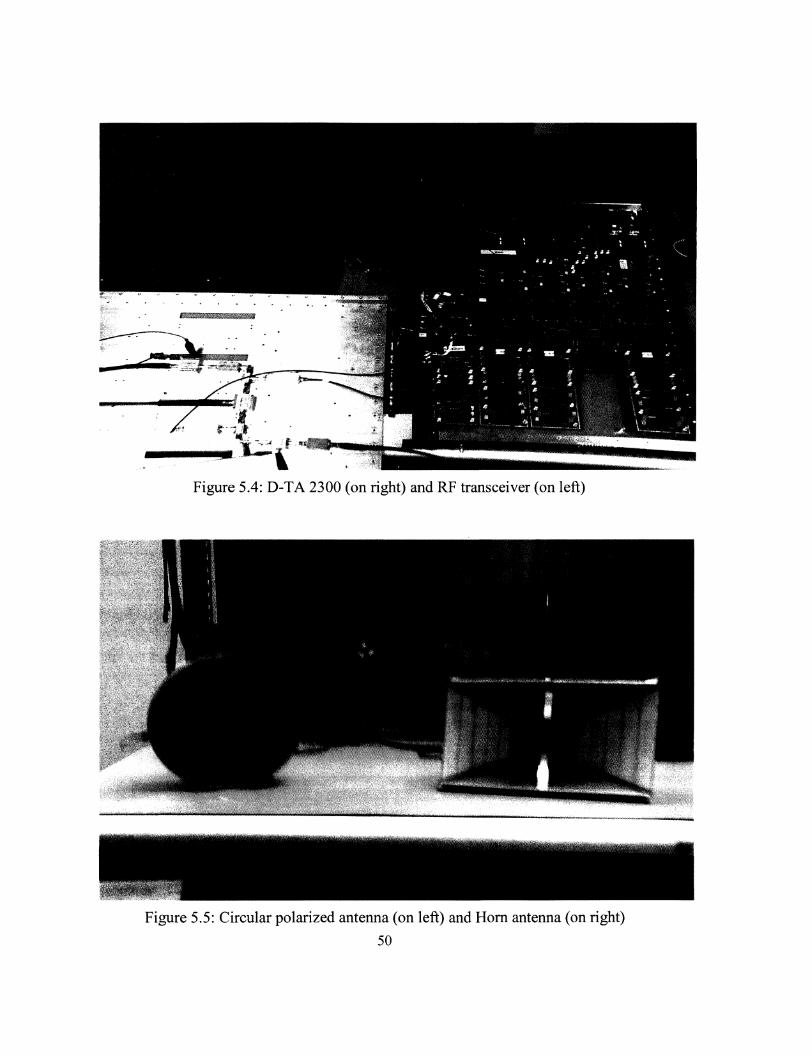
Figure 5.4: D-TA 2300 (on right) and RF transceiver (on left)

Figure 5.5: Circular polarized antenna (on left) and Horn antenna (on right)

50

Figure 5.4 shows the D-TA 2300 which is used to convert computer packets to an analog

signal centered at 70MHz and vice versa. It also shows the RF transceiver (on the left) which

is used to up-convert and down-convert signals from 70MHz to 1.5GHz and 1.5GHz to _

70MHz respectively. Figure 5.5 shows the horn antenna and the circular polarized antenna

used to transmit and receive signals respectively.

5.3 Resolution and Power Verification

The proposed waveform resolution is verified by detection of a rectangular metal object in an

office environment over various ranges for all three types of waveforms. The antenna used

for transmission is the H-1734 manufactured by BAE Systems. The H-1734 is a linear

polarized horn antenna with 8.65dB of bore sight gain at 1.5GHz. Figure 6.1 and 6.2 under

Appendix A show the antenna gain variation with target angle for the elevation and

horizontal planes respectively. The receiving antenna is the ASO-1658A which is a circular

polarized antenna with 2dB of bore sight gain at 1.5GHz [15]. Since the transmitting antenna

is linear polarized and the receiving antenna is cross-polarized, there is a 3dB loss in antenna

gain. This implies the antenna gain to be used in the range equation (1.10) is given by:

G = Gt + Gr — 6dB = 4.6SdB. The full system test is done in a closed stationery

environment and the transmit power can be observed from figure 5.3 to be -2.1dBm. Given

the above transmit power and antenna parameters used to conduct the experiment, the

expected maximum ranges for a single return with and without processing gain can be

calculated and the resulting values compared to the maximum range obtained from

51

correlation. Let the minimum target cross-section (a) be lm 2 , kT0 = —174dBm/Hz and

minimum SNR per pulse - (—) = 6.02dB. Since there is no pulse integration, n = 1. The \N/ i

Noise Bandwidth (Bn) and Noise Factor (Fn) are system parameters of the D-TA 3290 and

are given by 40MHz and 10 respectively. Maximum range without correlation gain is

obtained from equation 2.10 and is calculated as follows:

max (47r) 3*(3.981£-2l)*40£6*10*4 max

Maximum range with correlation gain is obtained from equation 2.14 and is calculated as

follows:

r^A 0.617?n*2.922*1024*0.2042 ^ _ r . „r

Rrnax = , ^ , ^ = > Rmax = 64 .76m. max (47T)3*(3.981£-21)*40E6*10*4 max

Based on calculations, a waveform with pulse compression can achieve a maximum range of

about 5.6 times the maximum range of a waveform without pulse compression. Due to test

environment limitations, the maximum range the target was able to reach was 9.8m.

However, the maximum range which can be obtained from auto-correlation can be observed

in figure 5.6. Figure 5.6 shows no returns above 40m and this value can be viewed as the

maximum range the system is able to process. The observed Rmax of 40 is smaller than the

calculated 64.76m value and this could be due to a smaller cross-section at the maximum

range than the estimated lm 2 value. The observed Rmax is however greater than the

calculated Rmax for a transmission scheme without pulse compression (11.45m) thus

validating the premise that pulse compression can reduce the required transmitter power.

52

Figures 5.6, 5.7 and 5.8 show range plots for the phase-coded-linear-FM waveform, phase

coded waveform and linear FM waveforms respectively. Table 5.1 shows normalized auto

correlation magnitudes of all three waveforms over various distances. Each figure shows

range returns for the target at two separate resolution bins where each resolution bin is 2.4m.

Given a 31.25MHz system bandwidth, the phase coded waveform is only able to achieve

9.8m of range resolution and this is observed by the superimposition of the range returns

shown in figure 5.5. The phase-coded-linear-FM signal is able to achieve the same range

resolution as the linear-FM waveform - 2.4m as shown in figure 5.6 and 5.8 respectively. In

this way, the range resolution advantage of frequency modulation is verified.

° t t I I I I I I I | I L _ 0 10 20 30 40 50 60 70 80 90 100

Figure 5.6: Plot of Auto-correlation against range for phase-coded-linear-FM waveform

53

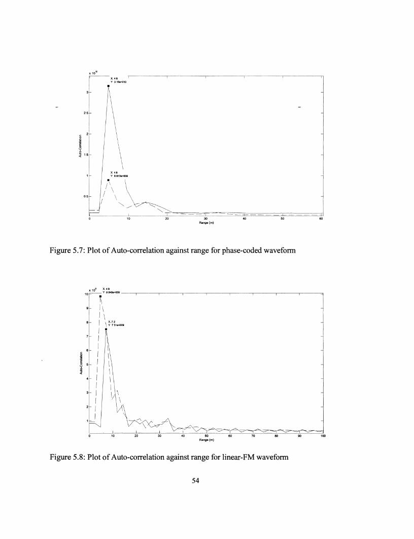
Figure 5.7: Plot of Auto-correlation against range for phase-coded waveform

Figure 5.8: Plot of Auto-correlation against range for linear-FM waveform

54

Phase-Coded-

Linear-FM

Distance (m)

Linear-FM

Distance (m)

Phase-Code

Distance(m)

2.4m

0.884(t)

0.892

0.836

0.731

0.946

0.955

2.4m

l(t)

0.99

0.791

0.858

2.4m

l(t)

1

0.832

0.923

0.95

4.8m

0.445

0.518(t)

0.448

0.463

0.815

0.739

4.8m

0.821

0.987(t)

0.0398

0.422

4.8m

0.803

0.819(t)

0.456(t)

0.669

0.706

7.2m

0.168

0.508

0.73(t)

0.907(t)

0.809

0.663

7.2m

0.673

0.787

0.545(t)

0.497(s)

7.2m

0.474

0.517

0.243

0.434(t)

0.464

9.6m

0.242(s)

0.233

0.443

0.471

0.21(t)

0.135(t)

9.6m

0.337

0.251

0.368

0.263(t)

9.6m

0.168

0.189

0.313(s)

0.23

0.199(t)

Table 5.1: Table of Normalized Auto-correlation values

55

Table 5.1 shows the normalized auto-correlation values for all three types of waveforms at

various distances or range bins. Values in table 5.1 with (t) next to them imply the location of

the metal box target while values with (s) imply correlation side-lobes. Due to the high _

clutter nature of the environment, returns exist at each range bin and the metal box can only

be clearly visualized at certain range bins. For both the phase-modulated-linear-FM and

linear-FM signals, the metal box auto-correlation peak is clearly visualized within the 7.2m

resolution bin. The phase-coded waveform only shows an auto-correlation peak within the

4.8m resolution bin due to the 9.8m resolution property of the waveform.

5.4 Doppler Verification

5.4.1 Doppler Test Setting

The ability of the radar system to distinguish stationery from moving targets depends on the

Doppler shift moving targets cause. The moving target used in this experiment is a

Powermax fan with Aluminum blades. The fan has four blades and each blade has a radius of

0.1778m. The transmitted signal hits the rotating blades which are moving perpendicular to

the direction of the signal. Figure 5.9 shows the cross-section diagram of the Powermax fan

blades. The echo at the receiver is a signal shifted by a Doppler which is proportional to the

radial velocity of the fan blades. Since radial velocity is directly proportional to the distance

from the center of the fan, each portion of the blade adds a Doppler shift which depends on

its distance from the center of the fan. This problem is minimized by using fan blades with

56

minimal cross-section around the center but increase as the fan edges are approached. Radial

velocity can be calculated with knowledge of the fan rpm as follows:

I arc = r9 =>

vr = ^ = r ^ = 2nr (rpm)/60 (5.0)

Where vr the radial velocity, r is the distance from the center to any point in the blade and

larc is the length of the arc made by any point on the blade as defined by its radius. Fan

speed is tested at two values of rpm - 1220 and 1517. From the above equation, the radial

velocity at the edge of the fan with radius of 0.1778m is calculated as follows:

0.1778(1220) 22.715m Vr_min = 2n *

60

vr_max = 2TT * °'17g10517) = 28.245m/s

The resulting Doppler frequencies are obtained from fd = vr * — and given a carrier

frequency of 1.472GHz, the minimum and maximum Doppler frequencies are calculated as

follows:

fdmin = 21.71 * i ^ = 111.46HZ

fd.max = 27.01 * i ^ ? = 138.59Hz

The calculated Doppler frequencies are as a result of velocities at the edge of the fan blades;

however, the maximum cross-section of the fan occurs at about half the length of the blades.

Since the cross-section is what dictates the strength of the echo, the most dominant Doppler

shift will occur at the point with the highest cross-section. This implies that the observable

57

minimum and maximum Doppler shifts will be about half the calculated values or 55.728Hz

and 69.295Hz for 1220rpm and 1517rpm respectively.

Figure 5.9: Cross-Section of Powermax fan

5.4.2 Doppler Test Results

Serial Doppler processing is done by taking the FFT of correlated values over successive

echoes at each range bin. The magnitude of the complex correlated values gives an indication

of the target range while the phase of the complex correlated values gives an indication of the

Doppler shift. Correlation improves the carrier to noise ratio (CNR) of the return while

preserving the phase such that fewer pulses are required to obtain the desired Doppler carrier

to noise ratio. To improve the correlation gain, the pulse repetition interval was increased by

a factor of 7 yielding a pulse repetition frequency (PRF) of 2.18kHz. Due to real time

processing restrictions, the maximum FFT length is 256 yielding a Doppler resolution of

58

8.5Hz. Figure 5.10 and 5.11 show the Doppler spectra at the fan range bin for rotating speeds

of 1220rpm and 1517rpm respectively.

40

30

£ 20

•4—»

S) 10 CD

-10

X:0 Y: 40.57 X: 59.6

Y: 30.32

X: 119.2 Y: 17.04

-1000 -800 -600 -400 -200 0 200 400 600 800 1000 Frequency (Hz)

Figure 5.10: Doppler spectrum at target range bin for fan rotating at 1220rpm

Figure 5.10 shows frequency components at DC, 59.6Hz and 119.2Hz. The DC component is

as a result of the stationery clutter present at the same range bin as the fan. The components

at 59.6Hz and 119.2Hz correspond to Doppler shifts produced by the center and edge radial

velocities respectively. The calculated Doppler shift due to the center radial velocity is

55.728Hz implying a discrepancy of 3.872Hz. Since the FFT resolution is 8.5Hz, the

discrepancy falls within the FFT resolution bin. The calculated Doppler shift due to the edge

radial velocity is 111.46Hz implying a discrepancy of 7.74Hz. 59

40

35

30

25

X:0 Y: 40.52 X: 68.12

Y: 30.33

X: 144.8 Y: 24.71

-1000 -800 -600 -400 -200 0 200 400 600 800 1000 Frequency (Hz)

Figure 5.11: Doppler spectrum at target range bin for fan rotating at 1517rpm

Figure 5.11 shows frequency components at DC, 68.12Hz and 144.8Hz. The DC component

is again as a result of the stationery clutter while the components at 68.12Hz and 144.8Hz

correspond to Doppler shifts produced by the center and edge radial velocities respectively.

The calculated Doppler shift due to the center radial velocity is 69.295Hz implying a

discrepancy between measured and calculated values of 1.175Hz which falls within the FFT

resolution bin. The calculated Doppler shift due to the edge radial velocity is 138.59Hz

implying a discrepancy of 6.21 Hz.

60

5.5 Tested Serial Vs Parallel Radar Processing

Experimental testing of the parallel process is done by multiplying the received sequence

from the rotating (fan) target with the transmitted sequence. Figure 5.12 shows both serial

and parallel processed Doppler spectra at the target range bin for the fan rotating at 1220rpm.

The serial Doppler spectrum is obtained by computing the FFT over 256 pulses while the

parallel Doppler spectrum is obtained by computing the FFT over 1024 pulses. Since 1024

pulses are utilized for the parallel process, the FFT length used to obtain the Doppler

spectrum is 1024 and the resulting frequency resolution is:

PRF 15 26/c

= —'•— = 14.9//z. For the parallel Doppler spectrum shown in figure 5.12, the

spectrum peak occurs at DC with a CNR of 33.19dB. The next predominant peak occurs at

119.2Hz with a CNR of 17.57dB. The observed edge Doppler shift coincides with that

obtained from serial processing and differs from the calculated Doppler shift of 111.46Hz by

7.74Hz. The CNR at DC as obtained by the serial process is 51.01dB while the CNRs at the

edge and center Doppler frequencies of the fan are 27.4dB and 38dB respectively as

observed from figure 5.12. Figure 5.13 shows both serial and parallel processed Doppler

spectra at the target range bin for the fan rotating at 1517rpm as obtained from 256 pulses for

the serial process and 1024 pulses for the parallel. For the parallel Doppler process, spectrum

peaks again occurs at DC and 149Hz with CNRs of 33.6dB and 25.03dB respectively as

observed in figure 5.13. The CNR at DC as obtained from the serial process is 51dB while

the CNRs at fan Doppler shifts of 68.12Hz and 144.8Hz are 38.39dB and 30.36dB

respectively as observed from figure 5.13.

61

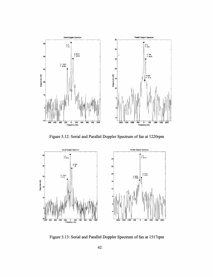
Serial Doppler Spectrum Parallel Doppler Spectrum

X -1448 Y 3036

X 6812 Y 38 39

-800 -600 -400 -200 0 200 400 600 800 1000 Frequency (Hz)

-2000 -1500 -1000 -500 0 500 1000 1500 2000 Frequency (Hz)

Figure 5.12: Serial and Parallel Doppler Spectrum of fan at 1220rpm

Serial Doppler Spectrum Parallel Doppler Spectrum

-1000 -800 -600 -400 -200 0 200 400 600 800 1000 Frequency (Hz)

-2000 -1500 -1000 -500 0 500 1000 1500 2000

Figure 5.13: Serial and Parallel Doppler Spectrum of fan at 1517rpm

62

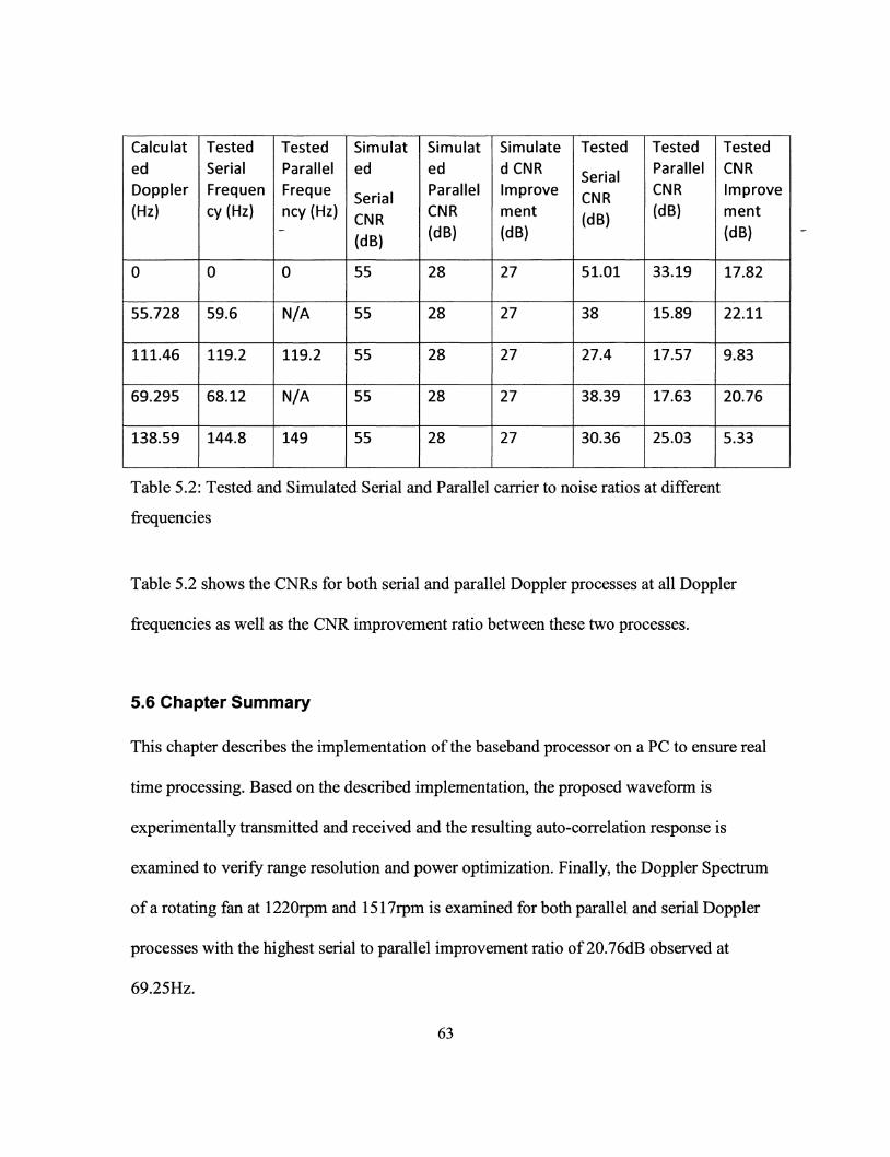
Calculat ed Doppler (Hz)

0

55.728

111.46

69.295

138.59

Tested Serial Frequen cy(Hz)

0

59.6

119.2

68.12

144.8

Tested Parallel Freque ncy (Hz)

0

N/A

119.2

N/A

149

Simulat ed

Serial CNR (dB)

55

55

55

55

55

Simulat ed Parallel CNR (dB)

28

28

28

28

28

Simulate dCNR Improve ment (dB)

27

27

27

27

27

Tested

Serial CNR (dB)

51.01

38

27.4

38.39

30.36

Tested Parallel CNR (dB)

33.19

15.89

17.57

17.63

25.03

Tested CNR Improve ment (dB)

17.82

22.11

9.83

20.76

5.33

Table 5.2: Tested and Simulated Serial and Parallel carrier to noise ratios at different

frequencies

Table 5.2 shows the CNRs for both serial and parallel Doppler processes at all Doppler

frequencies as well as the CNR improvement ratio between these two processes.

5.6 Chapter Summary

This chapter describes the implementation of the baseband processor on a PC to ensure real

time processing. Based on the described implementation, the proposed waveform is

experimentally transmitted and received and the resulting auto-correlation response is

examined to verify range resolution and power optimization. Finally, the Doppler Spectrum

of a rotating fan at 1220rpm and 1517rpm is examined for both parallel and serial Doppler

processes with the highest serial to parallel improvement ratio of 20.76dB observed at

69.25Hz.

63

Chapter 6

Discussion and Conclusion

6.1 Discussion

As shown in figure 5.6, the peak auto-correlation value for the phase-coded-linear-FM

waveform occurs at 7.2m and table 5.1 verifies this with a peak normalized auto-correlation

value of 0.907. Since targets at or below the smallest range bin (2.4m) are overshadowed by

the main beam interference, auto-correlation values at this range bin do not reflect the

presence of a target. From table 5.1, if the target is at 4.8m and the auto-correlation values at

the 2.4m range bin are ignored, a peak normalized auto-correlation value of 0.518 occurs at

4.8m. Based on the fact that the range bin with the peak auto-correlation value changes as the

target is moved across each range bin, it can be concluded that the phase-coded-linear-FM

signal has a resolution of 2.4m. From table 5.1, the peak auto-correlation value for the linear-

FM waveform occurs at 4.8m (ignoring values at 2.4m) with a peak normalized auto

correlation value of 0.987. From table 5.1, if the target is at 7.2m and the auto-correlation

values at the 2.4m range bin are ignored, a peak normalized auto-correlation value of 0.545

occurs at 7.2m. It can again be concluded that the linear-FM signal has a resolution of 2.4m

since the range bin with peak auto-correlation value changes as the target is moved across

each range bin. For the phase-coded waveform, the peak normalized auto-correlation value is

0.819 and it occurs when the target is 4.8m from the Radar. However, for subsequent pulses,

as the target distance from the radar is increased, the range bin with the peak normalized

64

auto-correlation value remains at 4.8m as can be observed from table 5.1. This means that the

phase-modulated signal has a range resolution which is greater than 9.6m.

As calculated in Chapter 5;~the rotating fan generates Doppler shifts at 55.728Hz,

111.46Hz, 69.295 and 138.59 and serial Doppler processing yields Doppler shifts which

differ from the calculated values by 3.872Hz, 7.74Hz, 6.21 Hz and 1.175Hz respectively. The

maximum deviation is less than the FFT resolution bin of 8.5Hz implying an acceptable

accuracy for experimentally determined values. Finer accuracy could be achieved by

increasing the FFT length. Parallel processing only yields Doppler shifts at the edge

frequencies of 111.46Hz and 138.59 with discrepancies of 3.872Hz and 10.41Hz

respectively. The discrepancies are again within the 14.9Hz frequency resolution for parallel

Doppler processing thus the Doppler accuracy is acceptable. Better accuracy can again be

improved by increasing the FFT length and number of pulses required for processing. The

inability of parallel Doppler processing to detect Doppler shifts resulting from the center of

the fan blades is as a result of the number of processed pulses. Increasing the number of

pulses will increase the FFT length and consequently the CNR at the Doppler frequency.

Table 5.2 shows the difference in CNR at the Doppler frequencies as obtained by the serial

and parallel processes. For simulated values, CNR is independent of the Doppler frequency.

The serial process yields a simulated CNR of 55dB while the parallel process yields a

simulated CNR of 27dB. This implies an improvement of 28dB of the serial process over the

parallel for the same processing speed. Table 5.2 shows the tested CNR improvement ratios

for all Doppler frequencies. The tested serial CNR at DC is 4dB less than the simulated value

and 17dB more than the parallel CNR. The tested serial CNR at Doppler frequencies due to

65

the center of the fan (55.73Hz and 19.296Hz) is 38dB which is about 17dB below the

simulated value and about 20dB above the tested parallel CNR. The 20dB improvement

factor between the serial and parallel process is reasonably close to the simulated 28dB value

and shows that serial processing yield a higher CNR than parallel processes for comparable

processing time. The difference between the simulated and tested CNR is because real

channel effects such as target cross-section, and actual antenna gain tend to increase the

signal attenuation. At edge Doppler frequencies of 111.46Hz and 138.59Hz, the parallel to

serial improvement factors are 9.83 and 5.33 respectively which are much lower than the

simulated 28dB value. However, the improvement factor still indicates that there is a

significant CNR benefit in using serial instead of parallel Doppler processing.

6.2 Conclusion

The main objective of this thesis was to come up with a Radar waveform which

requires low transmitter power, possesses fine range resolution and rejects ambiguous

targets. Another objective was also to examine the effect of parallel and serial Doppler

processing on the carrier to noise ratio. From Radar theory, it has been shown that minimum

transmitter power is obtained from continuous waveforms, however to achieve fine range

resolution, pulse compression is required. Chapter 2 of this thesis then examines frequency

and phase modulated waveforms as two types of compression schemes. The phase-modulated

waveform is theoretically shown to possess the ambiguous target rejection property while the

frequency modulated signal has the finer resolution of the two. By convolving the frequency

66

and phase modulated signals, a new waveform is obtained which has the fine resolution of

the FM signal and ambiguous target rejection property of the PM signal. Simulations are then

carried out (based on the proposed waveform) to test the ability of the receiver processor to

detect the range of a target and its speed in the presence of clutter, path loss, multipath, target

cross-section and AWGN. Target range is obtained by Auto-Correlation and ambiguous

target rejection is done by Cross-Correlation. Figure 5.6 verifies the resolution property of

the proposed waveform while figure 3.4 verifies the cross-correlation property. Simulation

also shows a 28dB benefit in CNR of serial Doppler processing compared to parallel Doppler

processing for comparable processing times. Experimental evaluation of the proposed

waveform is done by using the D-TA 2300 and D-TA 3290 which are IF and RF processors

respectively. The power benefit obtained by the pulse compression waveform is expressed in

terms of the maximum achievable range with and without pulse compression. Given the

hardware restrictions, the calculated maximum range without pulse compression is 11.45m

while the calculated maximum range with pulse compression is 64.76. From tested results

shown in figure 5.6, a maximum range of 40m can be observed from the auto-correlation

plot. This implies that for the same maximum range, a system which does not utilize pulse

compression requires greater transmitter power than a system that does. For range resolution

testing, a rectangular metal object is placed at various range bins and the Auto-Correlation

responses of all 3 types of waveforms are obtained. Figure 5.6 to 5.8 show that the phase-

coded-linear-FM signal has the same resolution as the linear FM signal - 2.4m while the

phase modulated signal has a range resolution greater than 9.6m. It was not possible to verify

ambiguous target rejection experimentally because for ambiguous targets to be detected, the

67

maximum range has to be greater than the unambiguous range. This condition was not

fulfilled in this case because the transmitted power was too small to detect any target over the

unambiguous range^ Doppler processing is done with a rotating fan as the target. The

Doppler velocities are calculated for rotating speeds of 1220rpm and 1517rpm and compared

with those obtained from the received echo. Serial Doppler processing yields CNRs at the

processed Doppler shifts which are about 20dB higher than those obtained from parallel

Doppler processing as shown in table 5.2. This indicates that for comparable processing

times, serial Doppler processing is better than parallel Doppler processing as the obtained

CNR at the Doppler frequency is considerably higher. This thesis has thus shown by

experimental evaluation that pulse compression in the presence of a continuous waveform

requires low transmitter power and achieves high resolution. Pulse compression also allows

for high CNRs when processing for Doppler as auto-correlation is used for echo compression

and this increases the SNR of the return signal.

Contributions made in this thesis include the derivation, simulation and testing of a

new waveform which rejects ambiguous targets and possesses high resolution. The resolution

property was verified through testing but the ambiguous target rejection property was not

because of transmitter power restrictions. Another significant contribution is the utilization of

auto-correlation values to obtain the Doppler shift in serial Doppler processing and the

resulting CNR improvement over parallel Doppler processes.

Further work in this research can be carried out in the waveform design by increasing

the peak to side-lobe ratio of the auto-correlation response. This can be done by utilizing

poly-phase codes instead of PN sequences as they possess a better peak to side-lobe ratio.

68

Side-lobe reduction in the linear FM signal can also be done by frequency weighting but at

the expense of lower range resolution. The demonstrated waveform in this thesis can thus be

improved by developing a coding scheme which has better cross-correlation and side-lobe

properties than PN sequences. Future work can also includes testing of the ambiguous target

rejection property of the waveform by utilizing more transmit power. Finally, the Doppler

test demonstrated in this research could be more definitive if the transmitted signal is focused

perpendicular to the edge of the fan blades such that a single Doppler frequency is obtained.

69

Appendix A

Antenna Measurements

Figure 6.1: Elevation plane Gain measurement for the H-1734 antenna at 1.5GHz

QQ

"0 3

0)

2° f r p-Ty-~fXT=::tpr • r y - p t p ..p pp- p. u_ • t=f=p=p i i , ! ! • ' - 1 - . I . i ' L " " : " " 1 " - !•""!"••

i s •— (— ———-j—s—~\~\~I—H—j—:—[—1—j———Ehi—r^F—^F\——i-

10 •—U — ^ h h H — ^ ~ r ^ ~ ^ " ~ H — n - r r h — k - k H — h h h ^ r h H — " __L_ _L_„L_L_L_ i— • l ~• • i | — h F r -H p>—r-r~\ r r f c p - ^ r " * ^ - F

I— [—[—j~H~ rhi——hr^"^^"1 ' •' P—z~^:~["~\'~\—hrr^~r"—r^

° ]' 1 ' 1111!' ,"U-'"'p: i i : ! r r r <\ r p ! rrr i r n

•w L_[_I—'—(—|—h"h"h"i——i—f--|—i—t—j—|—t~~ppppp!—hi—hH—hFh1-Fhppi •'

i s -|—|—|—rhrhhhh-h-4-L.L-H | t , L L L L L ^ - L L L L ^ L L L L I - L L L L L L ' " [ ' " ' I-- - - - - - - - - .. j j ! " J 1

20 -hhh,~hhhhhhh~h"hhhi~i ' 'i h^£hbFr^l~F^Frhhhhhhhhh p^p^pppppp_t^bp^^^ph r rp^p_ppphppht^t t t t t j :

^tttth^FhhhFp^hhhhthhb^ ppppcp FFEFBE, FEEEEEEB- pjpEf EEFEEEFfcEE& pbtFrEFF^FFÊE

00 MTk H ml'ttMril-Fr Ml hm EhEE EEEEEE E E E E E E E F E F E E B FEE-EEEEEEFEEU 3s • ^hb fbbbbbb -bbbhb i ^

LL^^^L^LLbt^ppLL j 4 i:bbLpbbbdzb|ztbbbbbbbbEbbr 4 0 1 1 I I 1 1 I I !;,...,L.L LI I I I 1:1 1 ! | 1: 1 \ \ \ \ 1 1 | M 1 1 | I I h

- - rbH H—j-rrrM—j-[-f--i— }-j * - ; F H - F - F H - ~ ! l | | 1 i ---4-U-k- b _ _ ^ i — i _ _ L _ i _ L — — [ _ — , _ ^ L L ^ L _ L _ _ ^ ^ L L _ J _ 4 4

:-j=bE- ~E- H-br- E-tbÊ tbi-E-pb E—--Urt=}4

:J|=E==j=^f=|E||S=^^p |=| j|J | :rgrF::Frr^^g|:F:E:N:r:F:Ffe

-_pLLpp-upH-h--|-+-pL-~LLL_L^—^r—r^-H—^^^hrrM^r

"TLEÊ' I r FM FF : frr r : FF F; r^FFFFH -: Ltui-t-: LuL-i-uuL LLQ-LLLLEL-LLULL LUI LLLL---"r~hhh^"b-^"rT~h —hb~bbbh^""hhh~b^—FFf-FF-FH-r-FFFF?-r--H ~! rrrFi h m ' i i L Frri i r r r r r FFTFT rF^rFFFFFt

^FIT r rnhi ' ' 1' 1 '^hi'^L : 1 ."[""'"" 11 [ 1 "T" ^ FFFFF' FFFF^f •FF-RFpFFhhT^F^FF-FFFFFbFFFt 1 i 4 [Mi hrnfflti : |F |F- | |=gE=^feFS •hK"RT- FFrh' FrrF-^F^F+ff F^P+F FFFFF-FFFR TrHTr FFri "Fnrr^rn^F+kr+r^FFFFFF^ r i m r rrrrTrrrrnn~rTrf"r^rH+rrrrrrhrrFr 1 1 \ \ \ | 1 1 1 1 : 1 1 i | > 1 If I i I { I ' » • ' tT-r pi FrFEFFFrl

-OO - 8 0 - 7 0 -SO -SO - 4 0 - 3 0 - 2 0 - I O iO 2 0 30 AO 50 60 70 80 90

Overlays H O R N _ 0 3 DAT-ant_under. H O R N _ 0 4 DAT-ant_under_te* t

Cal file units HORN_03 DAT dB i HORN_04 DAT dB i

A z i m u t h B e a m Peak Deg dB -0 33 8 65

-24 65 -18 63

( D e g )

Figure 6.2: Azimuth plane Gain measurement for the H-1734 antenna at 1.5GHz

QQ

0 -0 3

D)

ao p - , — r t T T T T T T T T T + l — 1 —

is •[ f i 1 M-hhh —i 10 •Pi[l.BiBffi-p 5 .tt±tLtt|=LL|.p:pip

L i_ i _)._•_—•— j—I—;_Fi-+-—F—f—

0 . tttE , t EpEE

_i5 |^ÊpEB^Êf£:

-20 - H — ! — h ^ h - — — h h h I '•—

n V: E -Ffc c -so •—! • j F 4 - * - F T - — - F F F ^ - r r

-35 -|—i * •[ | J^-l—LL .L. j . . j ] * f |-i—j—f—j—hhh ' 11 F

^ 0 Er-r fr-SEEB:EE£E

rtphpEpphbt^MT i l r FF

zJ-E^-EE-EpEL, 'LrFLLEt:-

rrû i ri M r • * \

FFFFFF^Fh-^r^-l

Bi|f]g

LL

Tr ^-U—i

—F—'

- •

-^

_ . L

+1

TM

- l ^ r .

M—i-

rr

1 -U-1 l

FtTl r f f t

:J4;rFF 1 1 : i hr

S .S SSLLEEEEP -L—pivLU-L-LLL

- — M — — r r a ~ *~*'rh

iEpftppEpE =FF#^FP

-pEErrE-r

44-- i j pp -^ps

ulFsuErit! -hF t^FF : ! - h F F S h r i

r L LF I~NH "hrrfi M

—rr rTr r

- so -eo -70 -eo - so -40 -so -20 -10 -o 10 20 30 40 s o e o 70 s o 90

A z i m u t h ( D e g )

Overlays HORN_01 DAT-ant_under_ HORN_02 DAT-ant_under_teat—-

Cal file units HORN_01 DAT dBi HORN 02 DAT dBi

Beam Peak Deg dB -0 29 8 97 17 38 -19 33

70

Bibliography

[1] Merrill I. Skolnik, Dean D. Howard, Radar Handbook, 2nd ed., McGraw-Hill, 1990,

pp. 18.46-18.50

[2] Merrill I. Skolnik, David J. Murrow, Radar Handbook, 2nd ed., McGraw-Hill, 1990,

pp.20.33-20.39

[3] Merrill I. Skolnik, Radar Handbook, 2nd ed., McGraw-Hill, 1990, pp. 1.1 -1.13

[4] Blake, L. V,: "A Guide to Basic Pulse-Radar Maximum-Range Calculation Part-1",

Naval Research Lab. Washington D.C. 20362, December 23rd 1969

[5] Merrill I. Skolnik, Lamont V. Blake, Radar Handbook, 2nd ed., McGraw-Hill, 1990,

pp.2.20 -2.26

[6] Merrill I. Skolnik, Edward C. Farnett and George H. Stevens, Radar Handbook, 2nd ed.,

McGraw-Hill, 1990, pp. 10.15-10.26

[7] Merrill I. Skolnik, William K. Saunders, Radar Handbook, 2nd ed., McGraw-Hill, 1990,

pp.14.21 -14.28

[8] G. L. Stuber, Principles of Mobile Communication, 2nd ed., Kluwer, Dordrecht, 2001,

Chapter 9.2

[9] Andrea Goldsmith, Wireless Communications, 1st ed., Cambridge University Press, 2005,

pp. 403-417

71

[10] Merrill I. Skolnik; William H. Long, David H. Mooney and William A. Skillman, Radar

Handbook, 2nd ed., McGraw-Hill, 1990, pp. 17.2 -17.18

[11] Merrill I. Skolnik, Lewis B. Wetzel, Radar Handbook, 2nd ed., McGraw-Hill, 1990,

pp.13.8-13.23

[12] http://www.windfinder.com/wind/windspeed.htm

[13] Rodger E. Ziemer and Roger L. Peterson, Digital Communications and spread Spectrum

Systems, Macmillan Publishing, 1985, pp.333-338

[14] Matteo Frigo and Steven G. Johnson, "The Design and Implementation of FFTW3",

Proceeding of the IEEE, vol. 93, no. 2, February 2005, pp. 216-231.

[15] Cobham Sensor Systems, "Spiral Antennas", Retrieved May 4th, 2010, from

https://www.cobham.com/media/101028/Spiral%20Catalog%20-%20Lansdale.pdf

72

http://www.windfinder.com/wind/windspeed.htm

https://www.cobham.com/media/101028/Spiral%20Catalog%20-%20Lansdale.pdf

Phase-Coded-Linear-Frequency- Modulated Waveform · PDF filewith the best mental and physical...

Documents

Transcript of Phase-Coded-Linear-Frequency- Modulated Waveform · PDF filewith the best mental and physical...