PHASE BEHAVIOR OF ETHYLENE/LOW-DENSITY POLYETHYLENE ...
68
PHASE BEHAVIOR OF ETHYLENE/LOW-DENSITY POLYETHYLENE MIXTURES by STEPHEN C. HARMONY, B.S. in Ch.E. A THESIS IN CHEMICAL ENGINEERING Submitted to the Graduate Faculty of Texas Tech University in Partial Fulfillment of the Requirements for the Degree of MASTER OF SCIENCE IN CHEMICAL ENGINEERING Approved of_th^ Committee # August, 1976
Transcript of PHASE BEHAVIOR OF ETHYLENE/LOW-DENSITY POLYETHYLENE ...

PHASE BEHAVIOR OF ETHYLENE/LOW-DENSITY
POLYETHYLENE MIXTURES
by
STEPHEN C. HARMONY, B.S. in Ch.E.
A THESIS
IN
CHEMICAL ENGINEERING
Submitted to the Graduate Faculty of Texas Tech University in Partial Fulfillment of the Requirements for
the Degree of
MASTER OF SCIENCE
IN
CHEMICAL ENGINEERING
Approved
of_th^ Committee #
August, 1976

f^Bu-i^e^
T3
ACKNOWLEDGEMENT
The author wishes to express his appreciation to the members
of his committee for their advice and constructive criticism through
out both the project and the writing of this thesis.
Also, the author acknowledges the National Science Foundation
for financial support of the project through grant ENG 74-09662.
11

TABLE OF CONTENTS
Page
ACKNOWLEDGEMENT ii
LIST OF TABLES v
LIST OF FIGURES vi
INTRODUCTION 1
Literature Cited 2
CHAPTER I CALCULATION OF PHASE EQUILIBRIA FOR ETHYLENE/LOW-
DENSITY POLYETHYLENE MIXTURES 3
Introduction 3
Polymer Solution Theory 6
Binary Mixtures 10
Chemical Potential 12
Determination of Characteristic Parameters 13
Calculations for Polydisperse Polymer Systems 21
Equilibrium Equations 21
Mass Balance 23
Algorithm for Solution of Simultaneous Mass Balance
and Equilibrium 25
Results 25
Conclusion 33
Recommendation 33
Literature Cited 34
CHAPTER II DESIGN OF A HIGH-PRESSURE PVT APPARATUS FOR POLYMERS 36
Introduction 36 iii

Page
Review of E:q)erimental Techniques 36
A PVT Apparatus for Liquid Polymers 42
Tenperature Control 45
Pressure System 45
LVDT and Micrometer Slide 45
Measurement of Volume Change 46
Data Correlation 47
Summary 49
Literature Cited 50
LIST OF REFERENCES 52
APPENDIX 55
The Determination of Characteristic Parameters 56
Specific Hard-Core Volume, v* 56
Characteristic Pressure, p* 56
Characteristic Tenperature, T* 57
Characteristic Parameters for Gases 57
Binary Interaction Parameter, p A 58
Literature Cited 58
IV

LIST OF TABLES
Table Page
CHAPTER I
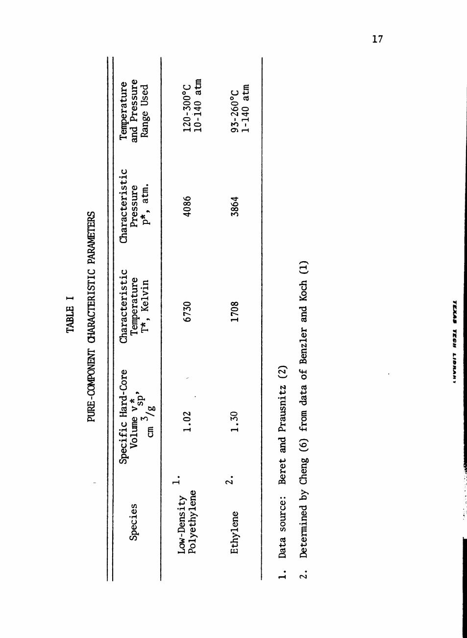
I Pure-Component Characteristic Parameters 17
II Phase Equilibrium at Design Conditions 28
III Conparison of Results of This Study with Results of Bonner et al. (5) 29
IV Comparison of the Calculated Resi4ts of This Study w i ^ the Data of Cheng ( 6 ) . . . . . . ". . . . . . . . 31
••?«-.

LIST OF FIGURES
Figure Page
CHAPTER I
1 Flow Diagram of Low-Density Polyethylene Manufacturing Process 4
2 Ethylene/Polyethylene Binary Coexistence Curve. . . 5
3 Thermal Expansion Coefficient vs. Tenperature for Low-Density Polyethylene 14
4 Theimal Pressure Coefficient vs. Tenperature for Low-Density Polyethylene 15
5 Calculated Temperature vs. Tenperature for Low-Density Polyethylene 16
6 Thermal Expansion Coefficient vs. Todperature for Ethylene 18
7 Thermal Pressure Coefficient vs. Tenperature for Ethylene 19
8 Calculated Tenperature vs. Tenperature for Ethylene 20
9 Algorithm for the Solution of Simultaneous Mass-Balance and Phase-Equilibrium Equations 26
10 Log-Normal Molecular Weight Distribution 27
CHAPTER II
1 A Typical Fluid-Displacement Apparatus 38
2 A Typical Piston-Displacement Apparatus 40
3 A Typical Bellows Apparatus 41
4 Modified Bellows End Piece 44
VI

INTRODUCTION
Mixtures of polydisperse low-density polyethylene and ethylene
are encountered over a wide range of pressures and tenperatures in
the low-density polyethylene manufacturing process. At pressures
below 1,000 atm, these mixtures will form two phases, one primarily
ethylene, the other primarily polyethylene. Since experimental data
on the compositions of these phases are limited, it is desirable to
develop a procedure for predicting the equilibrium conpositions.
In Chapter I we present an algorithm which can be used to predict
the conpositions of equilibrium phases in mixtures containing ethylene
and polydisperse low-density polyethylene. The use of the algorithm
requires pressure-volume-tenperature (PVT) data for the pure conponents
and limited interaction data for the mixture. Accurate PVT data exist
for many gases. Cheng (1) recently introduced an experimental tech
nique which can be used to obtain the necessary interaction data.
In Chapter II we present the design of an apparatus which can be
used to obtain the polymer PVT data.

Literature Cited
1. Cheng, Y. L., Ph.D. Thesis, Texas Tech University, (1976).

CHAPTER I
CALCULATION OF PHASE EQUILIBRIA FOR ETHYLENE/ LOW-DENSITY POLYETFIYLENE MIXTURES
Introduction
Low-density polyethylene is manufactured at tenperatures and
pressures as great as 260°C and 3,000 atm (18). Figure 1 is a flow
diagram of a typical low-density polyethylene-manufacturing process.
The mixture leaving the reactor, which typically contains 20 weight
percent polyethylene, is deconpressed to approximately 50 atm to separate
the unreacted ethylene from the polyethylene. Figure 2 is a typical
phase diagram for ethylene in equilibrium with low-density polyethylene
of a particular molecular weight. At sufficiently low pressures, the
mixture forms two phases, one primarily ethylene, the other primarily
polyethylene. In the manufacturing process, the ethylene phase is
purified to remove the low-molecular-weight polyethylene "waxes" and
"oils", conpressed, and recycled into the reactor.
Significant energy savings could be realized if the separation
step were accomplished at a higher pressure, reducing the energy
needed to recompress the recycled ethylene. At the higher pressures,
however, a sig^iificant amount of polyethylene will be present in the
ethylene-rich phase, and a significant amount of ethylene will be pre
sent in the polyethylene-rich phase. For the rational design of
energy-saving separation processes, the design engineer must be able

UJ CL Q
1 ^
3: + CM
£ ^ S
^
o ^ ~ ~
o —
CO
XD
^
11 CM
O
^
'
o \ os; ^ O Q. / ^ /
I-^ • ^
• - ^
'
,000
ps
i
o ^
1
> -
UJ a. Q
CO
O ^ 0 O O O to o ^ 1 ^ -J*
k
o 0 O LO
V .
1 ' O CO CO b
*
^
( CM
Tip
re
o o
CO Q.
O c a )
CJ ^
UJ Q. Q -J
O CJ
^ % :
n -CD J
^
CM o
O 00
/)
5
<D
r H
^ethy
ensity Pol]
Q CO
• * at O O
^ 2 O
Flow Diagram
(
Manufacturing
r-t
Figu:

o
3 U (D O c o + j <0 •H X <u o u fc-cd c: •H
/—> • M
•a •H
£ ^1 cd
m rH (U d (U
i - i >> s i H
3 O (U
f H
£ TS
g P E-« P^ '^^,
0) 1—»
• M
§ +J c/J
X c .c O +-> u w
•
0). ^ 3
N—^
UH
UJ+D ' 3dnSS3dd

to predict the effects of pressure and tenperature on the conpositions
of the two equilibrium phases.
In this work we show how the recently developed Cheng free-
volume theory of polymer solutions (6) can be used to predict phase
equilibrium between the polyethylene-rich phase (a) and the ethylene-
rich phase ($). The Cheng theory, unlike earlier free-volume theories
(10, 11, 12, 14, 19, 20) can be applied to gaseous as well as
dense liquid phases. We make use of the conputational algorithm of
Bonner et al. (5), which simultaneously solves equilibrium and mass-
balance equations, taking into account the molecular-weight distri
bution of the polymer. Sanple calculations are performed to illustrate
the use of the algorithm at design conditions.
Polymer Solution Theory S s
The first qualitatively correct theory of polymer solutions was ;
proposed independently in 1941 by Huggins (15) and Flory (8, 9). The
Flory-Huggins theory considers a polymer molecule as a chain of r
roughly spherical segments. By considering the number of ways the
polymer segments and solvent molecules can be arranged in a three-
dimensional lattice, the athermal entropy of mixing, also called the
combinatory entropy of mixing, is derived (8, 14)
In Equation (1), AS , is the athermal entropy of mixing, k is
Boltzmann's constant, N. is the number of molecules of conponent i,
I

'i "^i^i^^^l^l ^ ^T^^T) ^^ ^ ® volume fraction of conponent i, x. is
the mole fraction of conponent i, and v. is the molar volume of com
ponent i at system tenperature and pressure. In this and all following
expressions the subscript "1" refers to solvent and the subscript "2"
refers to polymer.
The Flory-Huggins theory is extended to non-athermal mixtures by
adding an enpirical van Laar enthalpy of mixing to -TAS , to obtain
the Gibbs energy of mixing (8, 14). Subsequent differentiation of the
expression for Gibbs energy of mixing gives the chemical potential of
the solvent,
(|i - yJ)/RT = ln((t)^) + (1 - l/r)(|>2 + x<^\, (2)
where y, is the chemical potential of the solvent in the mixture, y,
is the chemical potential of pure solvent at system tenperature and
pressure, R is the gas constant, T is the absolute tenperature, and
X is the Flory-Huggins interaction parameter. In the original develop
ment of the Flory-Huggins theory, x ^^s assumed to be independent of
concentration and proportional to 1/T.
The Flory-Huggins theory gives only a semi-quantitative represen
tation of the thermodynamic activity of polymer solutions. When x is
calculated from activity data, it is found in many cases to vary with
concentration (4, 14). x often does not vary with 1/T as proposed by
the van Laar model. Since the Flory-Huggins theory is based on the
rigid-lattice model, it gives no equation of state for the mixture.

8
A more exact representation of the properties of polymer solutions
is given by the free-volume or corresponding-states theory of Prigogine
(19, 20, 21) and Flory (10, 11, 13, 14). Prigogine and co-workers (19,
20, 21) viewed a polymer molecule as a chain of r segments, each having
3c external degrees of freedom. In the free-volume approach, a suitable
partition function is fonnulated for the mixture based on the Flory-
Huggins combinatory factor and a reasonable representation for the
intermolecular potential (10, 11, 13, 14). According to statistical
mechanics, the equation of state and all of the thermodynamic pro
perties can be derived from a partition function. Of particular interest
here are the equation of state
p(T.V3 = k T C ^ ) T , N '
and the chemical potential
0 u- " y-
kT f/9lnZ\ lim /31nz\ V 3N^ /T,V,N^ N - O V 8N^ /T,V,N^
(3)
(4)
vrfiere p(T,V3 is the pressure exerted by the N molecules at tenperature
T and volume V and Z is the canonical partition function.
The partition function proposed by Flory (10, 11, 13, 14) for
polymer solution is
Z = Z^^^(Xv*)N'^^(vl/^-l)^^^'^exp(Nrc/vT). (5)

where Z^^^^ is the combinatory factor, X is a geometric packing factor,
V* is the hard-core volume of a segment, v = v/v* = v /v is the sp sp
reduced volume, T = T/T* is the reduced temperature, v = V/Nr is the
volume per segment, v is the specific volume, v = v*N.r/M is the
specific hard-core volume, T* is the characteristic tenperature, N. is
Avagadro's number, and M is the molecular weight. Equation (5) yields
a reduced equation of state
pv _. y _ _ J.
T " W^ (6) vT
v^ere p = p/p* and p* is the characteristic pressure. The characteristic
parameters p*, v*, and T* are related by '(14) '
p*v* = ckT*. (7)
Equations (5), (6), and (7) are formally the same for pure conponents
and mixtures. When Equations (5), (6), and (7) are used for mixtures,
p*, V*, T*, c, N, and r are mixture properties which can be calculated
from the pure-conponent properties, as will be shown below.
In the derivation of the corresponding-states theory of Prigogine
and Flory, consideration was limited to dense, liquid phases. Cheng
(6) recently formulated a new partition function for pure conponents
and mixtures which overcomes this limitation. The distinguishing
feature of the Cheng partition function is based on a concept introduced
by Beret and Prausnitz (3). The contributions of the rotational,
vibrational, and electronic modes of motion to the partition function

10
vanish at the low-density limit. The partition function proposed by
Cheng is
^ = ^ c o * (Av*)'^-(vl/^-l)3Nr=(i)f^fr-« e:<p(Nrc/vT). (8)
From Equation (8) one obtains a reduced equation of state
IT re ~Zl7T~r " ^ ' ^^J (v' -1)
vdiere p, v, and T are defined as in Equation (6). The relationship
between the characteristic parameters p*, v*, and T* is given by
Equation (7). For a pure conponent. Equation (9) can be rewritten
using Equation (7) and the definition of v ,
Equation (10) reduces to the ideal-gas equation of state pMv /KT = 1 sp
at the low-density limit, making it equally applicable for dense and V
dilute phases.
Binary Mixtures
Following the development of Flory (13), Cheng (6) formulated a one-
fluid corresponding-states theory for binary mixtures of gases and liquid
polymers. The partition function remains the same as Equation (8),
with N, r, and c defined as follows:
N = N^ + N^
T p Mv (v - -1) vT

11
1 * 1 * 2 r r^ r^
^ = V l ^ V z '
* — (11)
Mihere f^ = r ^N /Crj Nj + r2N2) i s the segment fraction. The equation of
s ta te remains formally the same as Equation (9). Following Flory (13),
the character is t ic parameters for the mixture are
T* = —r-S^ iT-s- (12) *lPl/Tl * *2P2/T2
V* = v^ = V2 ,
irfiere 9. = s.r.N./(sTNTrT + s^N^r^) i s the segment fraction and s. is 1 1 1 1 ^ 1 1 1 2 2 2' ^ 1
the number of intermolecular contact s i t es per segment. The parameter
p,2 accounts for the intermoleciilar potential of binary interactions. * *
Note that the assumption v, = ^2 i s non-restr ict ive, since the size of
each segment may be a rb i t ra r i ly chosen. Due to this assumption, the
segpiKit ra t io T^/T^ i s given by
!l = ^!l!l4. (13) V2SP ^2
One must arbitrarily fix either r, or T2 to determine the other. We
have set r, equal to unity.

12
Using Eqiaations (7) and (13) , Equation (9) for the mixture be
comes
i^ _ RP*/ ' l ^ ^ 2 \, 1 1 ....
T ^ ^Vlsp V2sp^ ( -1) T
The reduced volume of the mixture can be obtained from the equation of
state. A good first approximation is:
V = vp v + 2^2 • (15)
Cheanical Potential
From Equations (4) and (8), the chemical potential of the solvent
is given by
0 * y. - Ui - V r - i _ A = ^,^ . (1 - r /r2)4'2 - ^
P 3—3f-
- 1/3 T V-, ' -1
ii^l-^i/r^)
^ p ,^4/3 ^ 4/3. 1 / p* 1 \ 1 P"
± * * ( W l . , ) i , ^ . , . ^ (,1/3.1)., 1/3
^ kT. ' 1 ^
* r 1 1 hi ®2
•u
V (16)
* * 1/2 * where X^2 " 1 " ^l/^2^P2 " ^^1/^2^ ^12* ^ similar expression,
given below, can be derived for the polymer chemical potential.

13
Detennination of Characteristic Parameters
The pure-component characteristic parameters can be determined
from experimental pressinre-volume-tenperature (PVT) properties (6,
10,12) by determining the best fit for the coefficient of thermal ex
pansion a, (1/V)(8V/8T) , the thermal pressure coefficient y, (3P/3T)y,
and the tenperature T. The characteristic parameters are assumed to
be constant over the range of pressures and tenperatures used in their
determination. The details of the procedure for determining pure-com
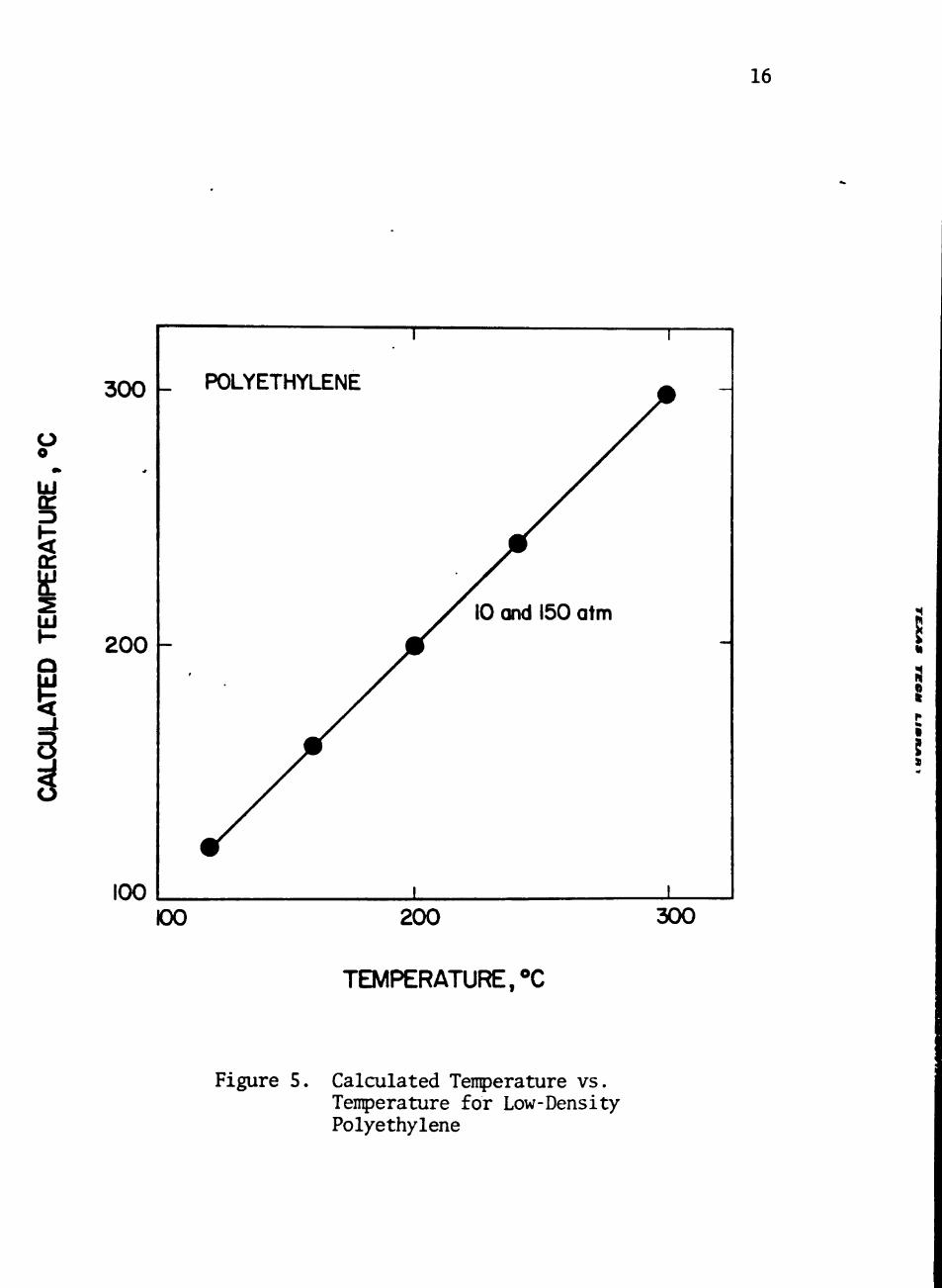
ponent characteristic parameters are given in the Appendix. Low-density
polyethylene parameters p*, v , and T* were determined using the data sp
of Beret and Prausnitz (2). The resulting correlations for a, Y» and
T are shown in Figures 3, 4, and 5. The derived characteristic para- F
meters are shown in Table I. Cheng (6) determined the characteristic
parameters for ethylene based on the data of Benzler and Koch (1).
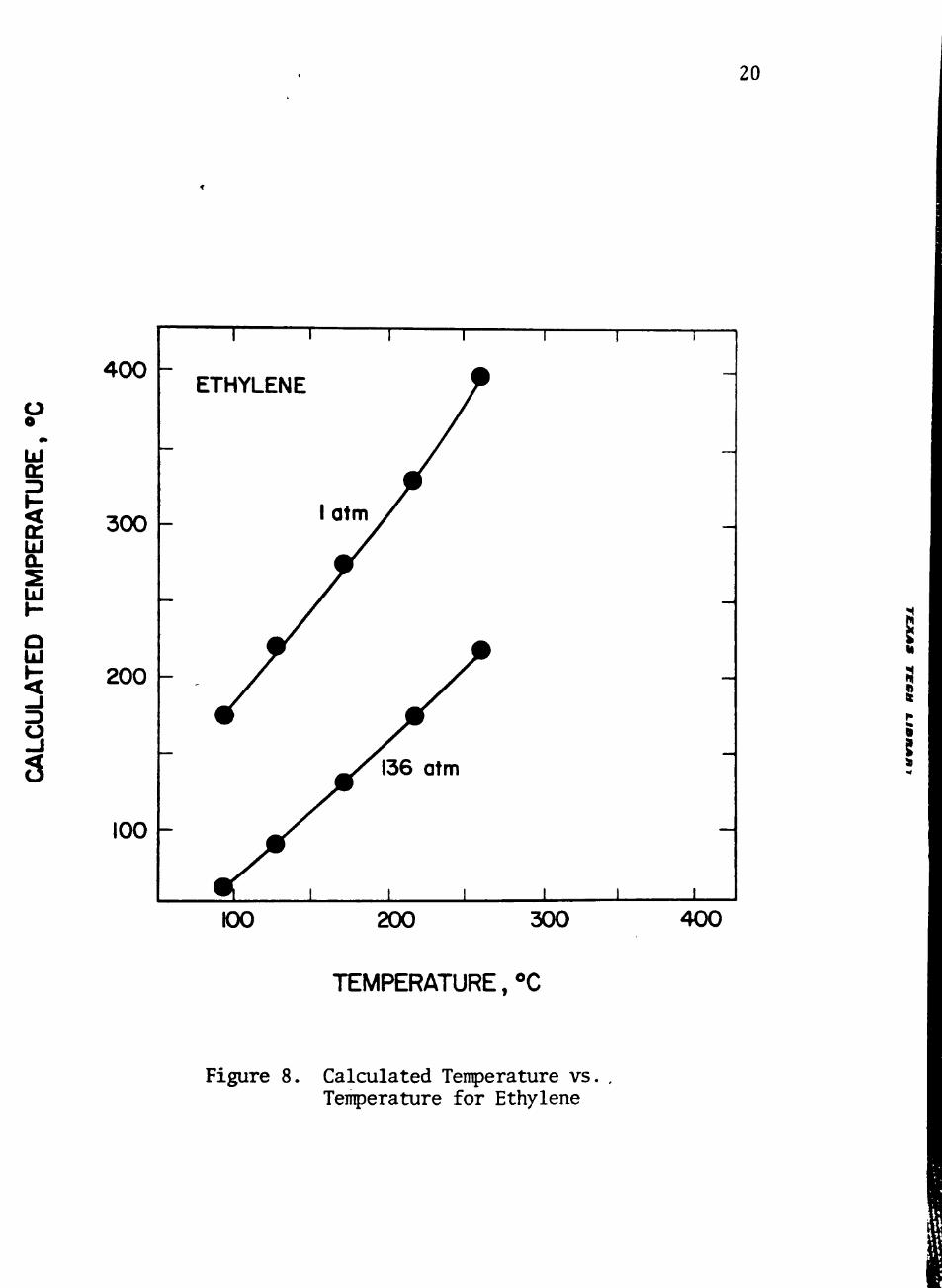
The resulting correlations are shown in Figures 6, 7, and 8, and the .
characteristic parameters are listed in Table I. The poor correlation
between calculated tenperature and actual tenperature shown in Figure
8 indicates that the van der Waals intermolecular potential used in
deriving the partition function [Equation (8)] does not describe the
behavior of gases well. The correlation in Figure 8 could be inproved
by utilizing a different form for the intennolecular potential at
the e^ense of greatly increased complexity. As will be seen, the
Cheng theory using the van der Waals potential accurately models the phase behavior of the ethylene/low-density polyethylene system.

14
O o uT
<
UJ o. UJ
(D
i-H
t O > s
rH
o
(A
I
in >
•H O
•H
o u g
•H
0}
to
0)
•H
,->t'^l«(D) 1N3I3IJJ30D N0ISNVdX3 lVWa3Hl

15
O o ill Q:
UJ o. UJ
I-
T H
(U
«-( o a.
•H to d
I
§
2 cd
>
•H
o •H
M-l
o CJ
to to a>
• H
^
I
(O lO
></uJiO • ( / ) lN3IOIJd300 3dnSS3dd HVIAIdBHl
16
O o
•»
UJ
(r
a: UJ
- 1
8
300
200
100
1
_ POLYETHYLENE
/
1
y / ^ 10 and 150 atm
1
1
«
r •
100 200 300
TEMPERATURE, X
Figure 5. Calculated Tenperature vs. Tenperature for Low-Density Polyethylene
17
H 4
to to to O fH (D
o • H 4-> to (D
• H fH W D 0) to ••-» to -
fH CU "^
e 4->
o
3 ' H >
Cd fH sS
to • H fH
•P
Cd & •> fH g *
o CJ
i •»
f H * to cd > CJO
<D r o •H 3 M-1 rH •H O
o> <D
CO
S
to
• H O
C/D
CJ o o o
+3 cd
o t o «?i-1
o (SI
i H 1
O
u o o
B +-> cd
vO O fS l
1 t o a\
'd-rH
1 I—1
vO 00
o 00 to
o to
OO
o
o o to
rsi
• H r-i
^ rH O O
S 0
rH
+->
CM
t4
•H
c 3
s
fH 0)
i H M
O
cd • p
•s cd fH
PH
T3
§ +J (U ^ 0
PQ
• • <u o s o to
Cd + j
^
o > m / - ^ vO
to P! (U
X u > .
Xi
T3
S •H g 0) • P
S
f
2
(NJ

1000 /K 18
0
—
o •;> E u O
ETH
YLEN
E
• E
XP
ER
IME
NT
— P
RE
DIC
TED
, \ij=
l3
-
1 1
2.5
1
«
• /
•
1
•
1
atm
^m
1
CVJ
1
• /
• /
/ i £ f w ^^
• o CO ro
1 1
1.5
ml
m
—
1
o in CM
o o CJ
-8
O o
•» UJ tr.
I UJ O.
S. UJ
O
Q o 0>
g rH >s p
w u o 4>
P Cd u
%
to >
•H o
•H MH m a> o u c o
•H to
8"
0)
fH
3> •H
f
0
I
O) 00 (D lO ro CVJ
X/000r( t ) ) 1N310133300N0ISNVcJX3 nVlNa3Hl

1000 atm/K 19
O o Ul cr.
cr Itl UJ
c 0
t H
P w u
p cd fH 0 i-0
to >
g •H O
•H M-l M-t 0 O
CJ 0
to to 0 fH
0
0
I •H
I n
>|/UJP0I *(> ) 1N3I0I333O0 3dnSS3dd lVl(Nd3Hl
20
O o UJ
Q:
Q:
Ul
UJ
o UJ
15
400
300
200
100
1 1 I \ 1
ETHYLENE P
/
l a t m X
- / /
^/^I36 atm
" y^
1 1
—
—
—
—
—
1 1
^
s
\
100 200 300 400
TEMPERATURE, ^0
Figure 8. Calculated Tenperature vs Temperature for Ethylene
21
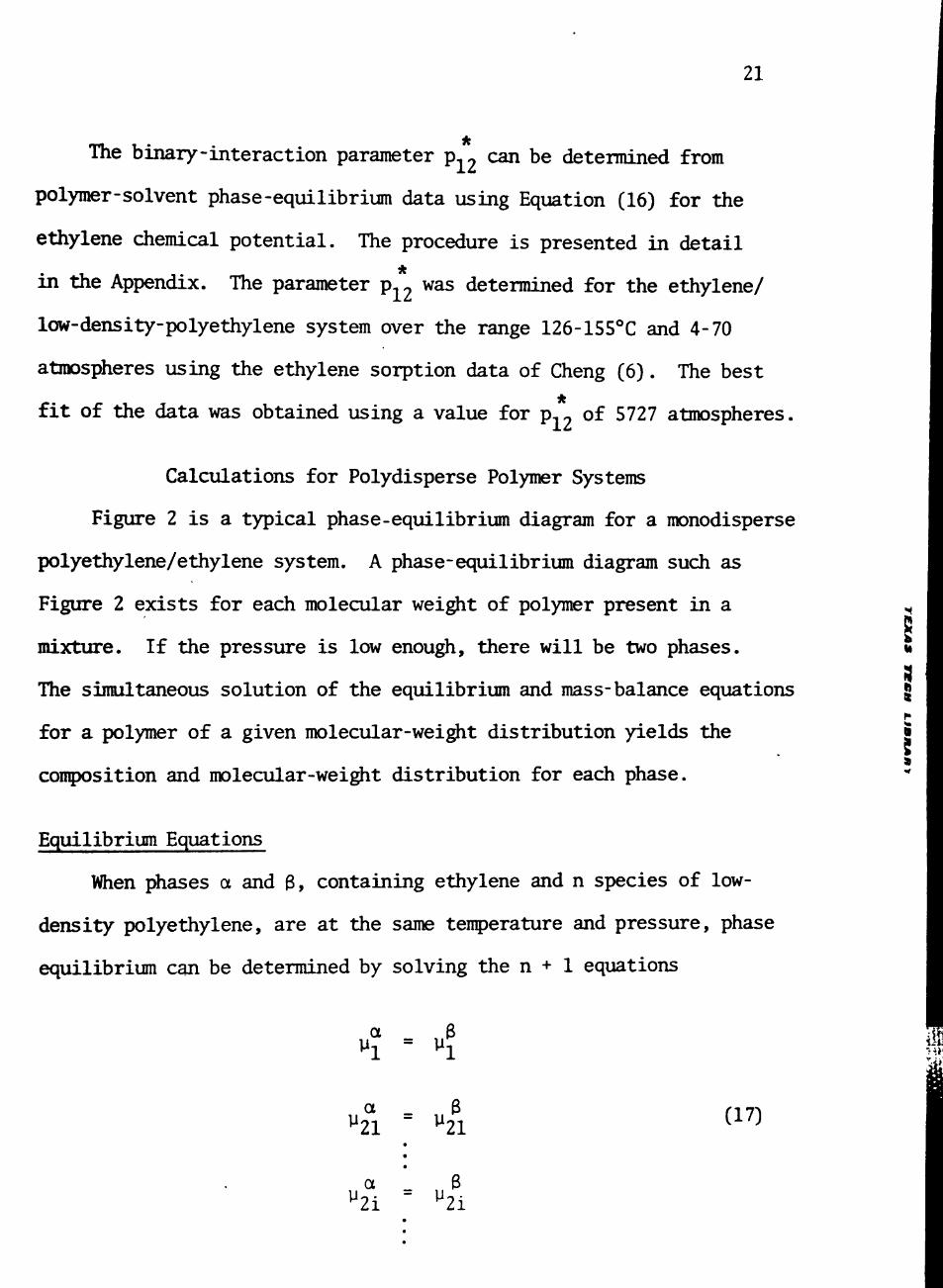
The binary-interaction parameter ip^^ ^ ^ t>e determined from
polymer-solvent phase-equilibrium data using Equation (16) for the
ethylene chemical potential. The procedure is presented in detail
in the Appendix. The parameter p, 2 was determined for the ethylene/
low-density-polyethylene system over the range 126-155*'C and 4-70
atmospheres using the ethylene sorption data of Cheng (6). The best
fit of the data was obtained using a value for p,2 of 5727 atmospheres.
Calculations for Polydisperse Polymer Systems
Figure 2 is a typical phase-equilibrium diagram for a monodisperse
polyethylene/ethylene system. A phase-equilibrium diagram such as
Figure 2 exists for each molecrular weight of polymer present in a
mixture. If the pressure is low enough, there will be two phases.
The simultaneous solution of the equilibrium and mass-balance equations
for a polymer of a given molecular-wei^t distribution yields the
conposition and molecular-weight distribution for each phase.
a
Equilibrium Equations
When leases a and 3, containing ethylene and n species of low-
density polyethylene, are at the same tenperature and pressure, phase
equilibrium can be determined by solving the n + 1 equations
IJ-a = y
3
y a 21 2 1
(17)
a 2i
= y 6 2i

22
a 3 ^2n = ^2n >
where the siperscripts refer to the a and 3 phases and the second sub
script refers to a polymer with a particular molecular weight. Equations
(17) can be rewritten by subtracting the pure-conponent chemical poten
tial (y?) from each side, resulting in:
(y, - y?)° = (y, - y?)^ (18a) 1 ^r 1 ^r
(y 21 O.a
U21) = • • •
O.a • • •
O.a *'2n) =
( ^ 1
(' 21
(^"211
0 , 6 • 1*215
0 , 8
0 , 8 - 1*2115 •
(18b)
(18c)
(18d)
(18)
f^2i
( 2n
Equation (16) can be used for the ethylene chemical potential if the
second term is modified to read [l-(r;j /(rPj )]'i'2» ^^®^® (^^n ^ ^ ®
number-average polymer chain length in the phase being considered.
The eciuation for the chemical potential of polymer species i of mole
cular weight M. is
1
^2i • '*2''i . i„ , . flii . l U V !2i e " *2i { r^ V 2 ^1
1 -(r,) 2-'n
^1^2i 4/3 ~ 4/3, ^ ^2 5

23
T\r573 ) • ^rn T^
(
P^1^2i - 1 ) l n ^
-1 - !|i (,i/3.„ . , 1/3, v ; ! ^21^1 V
P! ( "^2/
n (19)
viiere ^2^^ = p^ + (s2/s^)p* - 2(s2/s^)^/^p^*2, 21 is the segment fraction
of polymer species i, r2- is the chain length of polymer species i, and
n ^y - Z ^ 9-: is the total polymer segment fraction. ^ i=l ^^
We have assumed that pi, V2 * , and Tt are independent of polymer
chain length. Orwoll and Flory (17) show that this is a good assunption
provided that the polymer chain length is large. We also assume that
s^/s2 = 1. Estimates of s^/s2 based on lattice models and van der Waals
radii vary from 0.7 to 1.4, therefore the value s^/s2 = 1 provides a
reasonable estimate (5).
3
8
8
Mass Balance
The polymer molecular-weight distribution, which in fact consists
of a large number of discrete values, is commonly presented as a con
tinuous function w(M.) where 0 < M. < «>. In addition, the set of n + 1
simultaneous equations (18) would be very difficult to solve for large
values of n. We have therefore chosen to represent the molecular-weight

24
distribution as a continuous mathematical function, normalized so that;
w(M.)dM., (20)
where nu is the total polymer mass present.
A mass balance for each polymer species of molecular weight i
gives
ni5(M.) = m2(Mp/ 1. fi^'lyi V^(M,)A^^;w5,
(21)
,3 m^(M.) = m2(M^)/ ^^2^^iH/2N/"^ ' /^2^Y:2Y:::2\ (22)
where m2(M.) is the mass of polymer species i in phase a, m2(Mp =
m^(M.) + m^(M-) is the total mass of polymer species i, and H'2(Mj ) =
^i*.. The total mass of polymer in each phase is found by integrating
Equations (21) and (22) from M^ = 0 to M^ = «>.
m a - m2(M^)/ 1 +
2 1
dM. (23)
M
a ao 99
3 m. m2(Mp/ 1 +
/^>i^/^2Y "2 \ U5(MjyV^V - mV '>i^
dM., 1
(24)
The quantity H' (M.)/'i'°'( I-) can be determined from Equations (18c) and
(19) and the quantity H'?f/'i'? can be found using Equations (18a) and 16)

25
Algorithm for Solution of Simultaneous Mass Balance and Equilibrium
The algorithm used by Bonner et al. (5) to solve the simultaneous
mass-balance and phase-equilibrium equations is shown in Figure 9.
The value of (j^ in step 9 of Figure 9 can be determined from
( ^
r^v^ 1 2s
2^n '^ Vlsp
/Qw(M^)dM^
/QM">w(M^)dM.' (25)
The iteration is continued until m? from step 6 is equal to m? from
step 4 within a desired tolerance. The molecular-weight distribution
in each phase can then be calculated using Equations (21) and (22).
Results
The conputational algorithm of Bonner et al. (5) was used with
the Cheng free-volume theory to predict phase equilibria for the
ethylene/low-density polyethylene system. The molecular weight dis
tribution used was distribution w, of Koningsveld and Staverman (16),
shown in Figure 10. To illustrate the use of the algorithm for design
calculations, equilibrium phases were determined for a system with an
overall polymer concentration of 20 weight percent at 140° and 200°C
and 70, 150, .200, and 500 atm. The results of these calculations
appear in Table II. Equilibrium calculations were also performed
at 260*'C, 200, 500, and 900 atm, and 12.5% overall polymer concentration
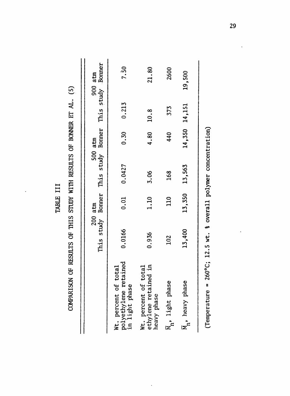
for conparison with the results of Bonner et al. (5). These results
and the results of Bonner et al. appear in Table III. A
final set of equilibrium calculations was made at 126° and 155°C,
h
i t

26
1. Assume a value of yl
I 2. Assume (l/r~) = 0 in
^ n Equations (10) § (18a)
J 3. Determine ^2 using
Equations (10) § (18a)
0^-1 ' y )
4. Calculate _a a ,3 .3
1'
m., nu, mr, and mz using
a ,3 »,3 2> "i i' ^2' K . 4'X. 'F:, Y^, and the characteristic
parameters from the definition of V
5. Calculate 'i'2(M^)/^2f^p using
Equation (18c)
I. Calculate m? from equation (23)
using nu from step 4
8. Calculate molecular-weight
distributions in both phases
using equations (21) § (22)
10. CalciiLate new
*2 ^°" (^n and(rp^
Calculate new
( T ^ ^ for each z n
phase using
Equation (25)
~l
Figure 9. Algorithm for the Solution of Simultaneous Mass-Balance and Phase-Equilibrium Equations
H

27
o o o lO 1 ^
O o o o lO
*•
J ^ iz o LU ^
(H < ^
33 O LJ - J o
c o
ibu
t
4-> V)
•H Q 4-)
•a •H
3
UJ
UJ
of lO LU
O Q.
(U
(30 o 1-4
• H
gOI ^ (IM)'^

28
TABLE II
PHASE EQUILIBRIUM AT DESIGN CONDITIONS
Tenperature °C
140
140
140
140
200
200
200
200
Pressure atm
70
150
200
500
70
150
200
500
B M , M„, n* n'
light heavy phase phase
0.00412 1.16
0.00403 3.04
0.00448 4.35
0.0166 14.6
0.00834 0.618
0.00752 1.71
0.0104 2.37
0.0221 9.36
50
51
55
122
72
70
83
134
13,259
13,254
13,258
13,353
13,319
13,304
13,334
13,404
(20 wt. % overall polymer concentration) A - Weight percent of total polyethylene retained in light phase B - Wei^t percent of total ethylene retained m heavy phase

o 2 2 •" C r II II
!2 ,#12^ II '"K ^ Z ^ M
i s IS Is
—
1
2 "O
2
CO CO <
2
27
o o o ir>~ r
O o o 0^ o
lO
000
««
lO OJ
• •
h~ zc iD ~ —
UJ ^
Q: <
" ^
o UJ
1 O 2 UJ 2 UJ
FHYL
UJ > -
_j o a.
,
c o
ibu
ti
: D
is
-a •H
^
cd
o
Mol
e
I-H
1 &
0.
Log-
1—1
(D
igur
U H
OJ
gOI ^ {IAI)M

28
Tenperature °C
140
140
140
140
200
200
200
200
TABLE II
PHASE EQUILIBRIUM AT DESIGN CONDITIONS
Pressure atm
70
150
200
500
70
150
200
500
A
0.00412
0.00403
0.00448
0.0166
0.00834
0.00752
0.0104
0.0221
B
1.16
3.04
4.35
14.6
0.618
1.71
2.37
9.36
M , n*
light phase
50
51
55
122
72
70
83
134
M , n'
heavy phase
13,259
13,254
13,258
13,353
13,319
13,304
13,334
13,404
(20 wt. % overall polymer concentration) A - Weight percent of total polyethylene retained in light phase B - Weight percent of total ethylene retained in heavy phase
29
a
LO
Cd O
PQ
O
P • M CO
0)
cd pq o o LO t
CO
to
o .LO
o 0 0
• r H
O O vO CM
o o LO
eg <^
to i H CM
•
o
o to
0 0 •
o i H
O OO
•
t o r** t o
o " ^ 'SJ-
LO i H
m •^ iH
O LO t o
m
CM "St O
VO o
0 0 vO
t o vO LO
*
to to
u <D
Bi cd CQ
o O >x CM T ^
B to
to • H X E-
tal
o 4->
t w
o +J
c <D U ^ <D
t H CD
• O
vO
i H O
• o
ined
cd
0 ^
a>
O to Cd
c .c <u i H
Pu > N 4 - >
^ ^ OO
D . 0 - H
• 4-> ^
r H
o P. c • H
tal
o tH • t H
t o O i
• o
• H
O T 3 +J
«4-l O
+-> c (U
u ^
<u
• H Cd •P 0 fH
0 to Cd
0 .C C 0
P . r H >>
• ->
^
J = +J
P H
^ cd 0
0 X
o t H i H
CM C i H
0 to Cd
JZ P H
+J
.c OO • H i H
M
i.^f=! IS
o LO t o
«k
t o i H
o o
• t o t H
0 to Cd
x: p.
& • cd 0
X •
i ^ f Is
cd
i
LO
CM
u o o vO CM II 0
Cd
0
i-0

30
11.2, 21.4, 38.4, and 52.0 atm, and 20% overall polymer concentration
for comparison with the data of Cheng (6). n,ese results appear in
Table IV with,the data of Cheng!
The results shown in Table II illustrate the equilibrium results
which can be expected when an industrial deconpression chamber is run
at various temperatures and pressures. At 70 atm, a pressure near
that used industrially, the light phase is essentially polyethylene-
free and the heavy phase contains only a small amount of the ethylene.
The number-average molecular weight in the heavy phase is nearly the
original value. As the pressure is increased to 150 and 200 atm,
the amount of polymer in the light phase remains nearly constant,
while the amount of ethylene in the heavy phase increases significantly.
The molecular-weight distribution remains roughly unchanged in both
phases. Increasing the pressure to 500 atm results in a large increase
in the amount of ethylene retained in the heavy phase and a significant
increase in the amount of polymer retained in the light phase. The
number-average molecular weight in the light phase increases substan
tially, which would have the result of changing the nature of the
secondary ethylene purification step in an industrial process. The
effect of increased tenperature on the results in Table II is an in
crease in the amount of polymer retained in the light phase, a de
crease in the amount of ethylene retained in the heavy phase, and an
increase in the number-average molecular weights in both phases.

31
TABLE IV
COMPARISON OF THE CALCULATED RESULTS OF THIS STUDY WITH THE DATA OF CHENG (6)
Tenp, **C
126
126
126
126
155
155
155
155
Pressure, atm
11.2
21.4
38.4
52.0
11.2
21.4
38.4
52.0
Wt. % ethylene This study
0.56
1.23
2.53
3.66
0.39
0.85
1.77
2.59
in heavy phase dieng
0.55
1.36
2.42 .
3.30
0.39
0.90
1.78
2.65

32
Conparison of the results listed in Table III shows close agree
ment between this study and the results of Bonner et al. at 200 atm.
At the higher pressures, howevet, the results differ markedly. The
difference illustrates the extreme sensitivity of free-volume polymer
solution theories to the values chosen for the characteristic para
meters. Bonner et al, derived the polyethylene parameters from the
low-pressure (40 atm) data of Orwoll and Flory (17). The interaction
parameter X, 2 was determined from the cloud-point data of Ehrlich (7),
vrtiich extend to 1760 atm. In contrast, the polyethylene data used
to derive the characteristic parameters used in this study extend to
900 atm (2), and the interaction data to 70 atm (6). Both studies,
then, are extrapolating much too far from the usable range of their
data in extending consideration to 900 atm. In addition, Cheng (6)
used ethylene data only up to 140 atm to determine the characteristic
parameters for ethylene. This was to assure conpatability with the
lower-pressure interaction data. The ethylene data (1) show a
marked change in the ethylene specific volume at around 300 atm. We
therefore recommend 300 atm as the maximum pressure for the use of
our characteristic parameters.
The results of the calculations below 70 atm, shown in Table IV,
show very good agreement with the data of Cheng. The maximum deviation
of calculated results from the data is 11%.

33
Conclusion
The Cheng theory of polymer solutions can be used, together with
a mass balance, to calculate phase equilibria for ethylene/low-density
polyethylene mixtures at the pressures and tenperatures used in the
separation step of the high-pressure manufacturing process. The
calculations consider the molecular-weight distribution of the polymer.
With the data considered in this study, accurate results can be ob
tained from 126-200°C and 0-70 atm. Use of the parameters derived
in this study is not recommended above 300 atm.
Recommendation
Accurate high-pressure binary phase equilibrium data are needed
for the ethylene/low-density-polyethylene system to extend the re
sults of this study to higher pressures.

Literature Cited
1. Benzler, H., and A. V. Koch, Chem.-Ing.-Tech., 27 , 71 (1955).
2. Beret, S., and J- M. Prausnitz, Macromolecules, 8, 536 (1975).
3. Beret, S., and J. M. Prausnitz, A.I.Ch.E. J., 21 , 1123 (1976).
4. Bonner, D. C , and J. M. Prausnitz, A.I.Ch.E. J., 1£, 943, (1973).
5. Bonner, D. C , D. P. Maloney, and J. M. Prausnitz, I E.C. Process Design and Development, 15, 91 (1974).
6. Cheng, Y. L., Ph.D. Thesis, Texas Tech University, (1976).
7. Ehrlich, P., J. Polym. Sci. Part A, _3, 131 (1965).
8. Flory, P. J., J. Chem. Phys., 9, 660 (1941).
9. Flory, P. J., J. Chem. Phys., 1£, 51 (1942).
10. Flory, P. J., R. A. Orwoll, A. Vrij, J. Amer. Chem. Soc, 86, 3507 (1964).
11. Flory, P. J., R. A. Orwoll, A. Vrij, J. Amer. Chem. Soc, 86 , 3515 (1964).
12. Flory, P. J., and A. Abe, J. Amer. Chem. Soc, 86 , 3563 (1964).
13. Flory, P. J., J. Amer. Chem. Soc, 87_, 1833 (1965).
14. Flory, P. J., Disc. Faraday Soc, 49 , 7 (1970).
15. Huggins, M. L., J. Chem. Phys., 9, 440 (1941).
16. Koningsveld, R., and A. J. Staverman, J. Polym. Sci. Part A-2, 6, 305 (1968).
17. Orwoll, R. A., and P. J. Flory, J. Amer. Chem. Soc, 89, 6814 (1967).
18. Platzer, N., Ind. Eng. Chem., 62 , 7 (1970).
19. Prigogine, I., N. Trappeniers, and V. Mathot, Disc. Faraday Soc,
15 , 93 (1953).
34

35
^^' 559^(1953) ^" * ' '' PP '' '' ' ^^ - ^ ^ ° ^ ' J. Chem. Phys., 21,
2^- ?,^j??g^^» I'* The Molecular Theory of Solutions. North Holland Publishing Co., Amsterdam (1957). ""

CHAPTER II
DESIGN OF A HIGH-PRESSURE PVT APPARATUS FOR POLYMERS
Introduction
In Chapter I we presented a procedure for the calculation of
equilibrium phases for systems containing ethylene and low-density
polyethylene, based on the Cheng theory of polymer solutions (6)
and the work of Bonner et al. (2). For calculations involving
binary mixtures, the Cheng theory requires the use of accurate pres
sure-volume-tenperature (PVT) data for both pure conponents, as well
as interaction data for the mixture. Accurate PVT data already
exist for many gases. Cheng (6) has developed an experimental pro
cedure for obtaining the necessary interaction data. Relatively
few polymers have been accurately characterized.
In this study we explore the methods available for the determin
ation of PVT properties for liquid polymers. We present an experi
mental apparatus which is a modified version of the apparatus used
by Quach and Simha (18, 19), and discuss how experimental data from
such an apparatus can be used to derive the quantities needed for
use with the Cheng theory.
Review of Experimental Techniques
Many studies have been made on the effect of pressure and
tenperature on polymer densities. Of the methods used, three can
36

37
be applied to the liquid state. These are the fluid-displacement
method ( 9 , 10, 12, 17, 28), the piston-displacement method (4, 5, 7,
8, 11, 15, 24, 27, 29, 30, 31, 32), and the bellows method (1, 3,
16, 18, 19).
Figure 1 illustrates a typical fluid-displacement apparatus.
The polymer sanple is contained within a small chamber with a single
exit which leads to a capillary. The sanple is surrounded by a con
fining fluid, such as mercury, which fills the remainder of the chamber
and extends into the capillary. Changes in the volume of the con
fining fluid and polymer sample are followed by observing the changes
in the height of the confining fluid column within the capillary.
Pressure is transmitted to the sample through the confining fluid, ] *
which contacts the hydraulic oil of the pressure generation and measure- ,
ment equipment at its upper interface. For temperature control the |
apparatus can be immersed in a constant-tenperature bath or surrounded I
by heating elements.
The distortion of the fluid-displacement apparatus with pressure
can be easily compensated for by calibration with a fluid whose PVT
properties are known. When liquid-polymer densities are to be deter
mined, provision must be made to keep the polymer sanple from escaping
the cell. There is a possibility of interactions between the sample
and the confining fluid, especially at high pressures. Since no
data exist on these interactions, they must be assumed to be negligible,
leading to errors of unknown magnitude.

38
CAPILLARY
SAMPLE CHAMBER
TO PRESSURE GAUGE
HYDRAULIC OIL
CONFINING FLUID
POLYMER SAMPLE
Figure 1. A Typical Fluid-Displacement Apparatus

39
Figure 2 shows a typical piston-displacement apparatus (5). The
polymer sample is placed in a cylindrical chamber which is mated with
a closely-fitting piston. Pressure is applied to the sanple by exerting
force on the piston. The force can be supplied by a Universal Testing
Machine (7, 15, 24, 27, 30), a system of weights (5), or a second cylinder
connected to pressure generation and measurement equipment (8, 29).
Tenperature control is achieved by surrounding the cylinder assembly
with heating elements or by submerging the assembly in a constant-
tenperature bath. The change in volume of the polymer sanple is deter
mined from the movement of the piston.
To obtain accurate results with the piston-displacement method,
one must compensate for the conpression of the piston, the initial
slack in the system, the expansion in length and cross-sectional area
of the cylinder, and the friction between the piston and the cylinder
(11). Nfolten polymer will be extruded through the piston-cylinder
clearance, especially at high pressures. Some investigators (8, 27)
attenpt to correct for this by subtracting the mass of the extruded
polymer from the sanple mass, though this can lead to errors at the
lower pressures.
The most recently developed method for polymer density deter
minations is the bellows method of Quach and Simha (18, 19), based
on Bridgman's apparatus for fluids (3). In the bellows apparatus,
shown in Figure 3 (18), the polymer sanple is sealed inside a flexible
metal bellows along with a confining fluid. When the bellows is ex-

40
-OftL INOlCATOft
-WClGMT
-STEEL PISTON
- S T E E L BARREL
i i i ^ -MEAT
V • J
ERS
-INSULATION
- p t u e
i >;- - POLYMER
-PLUO
\ 1 ( • «
1
Figure 2. A Typical Pis ton-Displacement Apparatus [After Chee and Rudin (5)]

41
PRESSURE
INLET
PISTON
BACK-UP RING
MICROMETER SLIDE
HIGH-PRESSURE
TUBING
PRESSURE CELL
STAINLESS-STEEL ROD
BELLOWS
END PIECE
CLAMP
O-RING
Figure 3. A Typical Bellows Apparatus [After Quach (19)]

42
posed to external hydrostatic pressure, it contracts until the pressure
of the sanple inside the bellows balances the applied pressure. Since
the effective cross-sectional area of the bellows remains constant
under isothermal conpression (3, 18, 19), the volume change of the
combined sample and confining fluid can be obtained from the change in
length of the bellows. The bellows is constrained to linear motion by
a piston moving in a closely-fitting sleeve. The length change of the
bellows is measured with a linear variable differential transformer
(LVDT). The core of the LVDT is connected to the piston by a non
magnetic stainless-steel rod, and the coil of the LVDT, separated
from the core by non-magnetic high-pressure tubing, is connected to
the moving member of a precision micrometer slide. Tenperature con
trol is achieved by immersing the apparatus in a constant-tenperature
bath.
The bellows method gives accurate results when the apparatus
is calibrated with fluids of known PVT properties. The primary dis
advantage of the bellows method is the possibility of interactions
between the confining fluid and the polymer at high pressures.
A PVT Apparatus for Liquid Polymers
Our apparatus is based on the bellows apparatus of Quach and
Simha. The lower bellows end piece has been modified to allow the
polymer sample to be loaded into the bellows without the use of a
confining fluid. The closure for the pressure cell has been incor
porated into the lower bellows head. Finally, the piston on our

43
apparatus has been designed to make minimum contact with the cylinder
wall to avoid the friction problem encountered by Quach (20).
Figure 4 shows the modified bellows end piece. The bellows end
piece incorporates a valve assembly to facilitate the evacuation of
the bellows. The valve packing assembly consists of a Teflon packing
disc with two brass followers. The valve stem has a 59° included
angle which mates with the 60° included angle of the valve seat. The
valve assembly has been leak tested at 10,000 psia.
The bellows assembly is loaded as follows:
(1) The valve stem, packing, and packing nut are
removed from the end piece (Figure 4a).
(2) The bellows is extended until the volume inside
the bellows corrugations is equal to the total volume
of the relaxed bellows.
(3) A weighed amount of polymer, calculated to fill
the relaxed bellows exactly, is loaded into the bel
lows.
(4) The valve stem, packing, and packing nut are
installed, with the packing conpressed and the valve
stem_ retracted (Figure 4b).
(5) The bellows is evacuated through the side
opening in the end piece.
(6) The valve stem is tightened while the bellows
is evacuated.

PACKING ASSEMBLY
44
(4a)
VALVE STEM
PACKING NUT
(4b)
BELLOWS END PIECE
T
i l l
i , • • •
(4c)
Figure 4. Modified Bellows End Piece
45
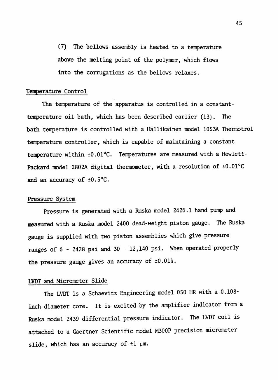
(7) The bellows assembly is heated to a tenperature
above the melting point of the polymer, which flows
into the corrugations as the bellows relaxes.
Tenperature Control
The temperature of the apparatus is controlled in a constant-
tenperature oil bath, which has been described earlier (13). The
bath tenperature is controlled with a Hallikainen model 1053A Thermotrol
tenperature controller, which is capable of maintaining a constant
tenperature within ±0.01°C. Temperatures are measured with a Hewlett-
Packard model 2802A digital thermometer, with a resolution of ±0.01°C
and an accuracy of ±0.5°C.
Pressure System
Pressure is generated with a Ruska model 2426.1 hand punp and
measured with a Ruska model 2400 dead-weight piston gauge. The Ruska
gauge is supplied with two piston assemblies which give pressure
ranges of 6 - 2428 psi and 30 - 12,140 psi. When operated properly
the pressure gauge gives an accuracy of ±0.011.
LVDT and Micrometer Slide
The LVDT is a Schaevitz Engineering model 050 HR with a 0.108-
inch diameter core. It is excited by the amplifier indicator from a
Ruska model 2439 differential pressure indicator. The LVDT coil is
attached to a Gaertner Scientific model M300P precision micrometer
slide, which has an accuracy of ±1 ym.

46
Measurement of Volume Change
The operational procedure for our apparatus is the same as the
procedure used by Quach and Simha (18, 19). The volume change is
measured by a combination of the micrometer slide reading and the LVDT
output. At constant tenperature and atmospheric pressure, the micro
meter slide is adjusted until the anplifier indicator reads zero, in
dicating that the LVDT core is centered within the coil. The initial
reading M . of the micrometer slide is noted. When pressure is appliedj
causing the bellows to contract, the core moves in relation to the
coil, causing a non-zero reading on the anplifier indicator. The
micrometer slide is adjusted to obtain another zero reading and an
other micrometer reading M is taken. The absolute value of the dif
ference between the micrometer readings is given by the equation
|M - MQI = AL + AJl , (1)
where AL is the change in length of the bellows and M is the change
in length of the other parts of the apparatus. The total volume
change of the polymer with respect to the volume at atmospheric pres
sure is
where W is the mass of polymer in the bellows, v ^ is the specific
volume of the polymer at atmospheric pressure and system temperature,
V is the specific volume of the polymer at system pressure and

47
tenperature, and A is the effective cross-sectional area of the bellows.
Substitution of Equation (1) into Equation (2) yields
A(|M - M^I - A£) ^spo - ^sp = :^ (3)
The quantities A and A£ can be obtained from calibration using mercury
and benzene (18). The tenperature dependence of A is obtained from
the theimal expansion coefficient of the bellows material (18, 19).
Since the foregoing method measures only the quantity v ^-v ,
V Q must be obtained as a function of tenperature. The bellows appara
tus can be used to obtain the value of v ^ relative to the specific
volume at a reference tenperature (18, 19). The specific volume at
the reference tenperature must be obtained by an independent method.
Data Correlation
To determine the characteristic parameters for the Cheng free-
volume theory, the specific volume v , the thermal expansion coefficient
a, (1/V)(3V/3T) , and the thermal pressure coefficient y , (9P/3T)^,
must be known for the polymer as functions of tenperature and pres
sure. These properties can be determined by fitting the PVT data to
an appropriate equation of state and differentiating the equation of
state.
The Tait equation (25, 26) has been shown to give a very accurate
representation of the PVT behavior of polymers at high pressure (14).
The Tait equation gives the quantity v /v Q as

48
V ^ = 1 - C ln(l + p/B), (4) spO
where C is a constant, p is the pressure, and B is a function of tem
perature. Simha et al. (19, 23) have shown that the tenperature
dependence of B can be expressed by
B = b^ exp (-b2T), (5)
where b, and by are constants and T is the tenperature. The quantities
C, b,, and b2 can be determined from a non-linear regression fit of
the specific-volume data. Simha et al. (21, 22) have shown that the
tenperature dependence of the specific volume at atmospheric pressure
can be given by an expression of the form:
^ ^ p O = J"^^^ * E • (6>
where D and E are constants. The values of D and E can be determined
3/2 from a linear least-squares regression fit of In v Q VS . T
The differentiation of Equation (4) gives
a = aQ + ^ ^ [1 - C ln(l + p/B)]'^ (7)
and
Y = ap (E^)[l - C ln(l * p/B)] * p ^ , (8)
where a« is the coefficient of thermal expansion at atmospheric

49
pressure and system temperature. The differentiation of Equation (5)
yields
dlnB , •Ifr = -^2 • C9)
The value of a^ can be determined from differentiation of Equation (6)
% = |DT^^^- (10)
Substitution of Equations (9) and (10) into Equations (7) and (8)
yields
T 1/0 pCb^ ^
and
Y = |nr^/^(2;?.)[l - C ln(l + p/B)] - pb^. (12)
Summary
A higji-pressure apparatus is now available at Texas Tech
University for determination of densities of liquid polymers. The
design of the apparatus is based on the bellows apparatus of Quach
and Simha, modified so that the use of a confining fluid is no longer
required. The operating range of the apparatus is 0 - 10,000 psia
and 25 - 250°C.
TEXAS TECH LibhARY

Literature Cited
1. Beret, S., and J. M. Prausnitz, Macromolecules, 8 , 536 (1975).
2. Bonner, D. C , D. P. Maloney, and J. M. Prausnitz, Ind. Eng. Chem. Process Design and Development, 13, 91 (1974).
3. Bridgman, P. W., Proc. Am. Acad. Arts § Sci.. 66 , 185 (1930).
4. Bridgman, P. W,, Proc. Am. Acad. Arts ^ Sci., 76, 71 (1948).
5. Chee, K. K., and A. Rudin, Ind. Eng. Chem. Fund., 9, 177 (1970).
6. Cheng. Y. L., Ph.D. Thesis, Texas Tech University (1976).
7. Chung, C. I., J. Appl. Polym. Sci., 15 , 1277 (1971).
8. Foster, G. N. Ill, and R. G. Griskey, J. Sci. Instrum., 41, 759 (1964).
9. Gubler, M. G., and A. J. Kovacs, J. Polym. Sci., 34., 551 (1959).
10. ffellwege. Von K. H., W. Khappe and P. Lehmann, Kolloid Z. U. Z. Polym., 183, 110 (1962).
11. Heydemann, P. L. M., and J. C. Houck, J. Polym. Sci. Part A-2, 10, 1631 (1972).
12. Rmter, E., and W. G. Oakes, Trans. Faraday Soc, 41 , 49 (1944).
13. Lawrence, R. G., M. S. Thesis, Texas Tech University (1970).
14. Maloney, D. P., and J. M. Prausnitz, J. Appl. Polym. Sci., 18, 2703 (1974).
15. I^tsuoka, S., and B. Maxwell, J. Polym. Sci., 32 , 131 (1958).
16. Olabisi, 0., and R. Simha, Macromolecules, 8, 206 (1975).
17. Parks, R. W. and R. B. Richards, Trans. Faraday Soc, 45 , 203 (1949).
18. Quach, A., Ph.D. Thesis, Case Western Reserve University (1971).
19. Quach, A., and R. Simha, J. Appl. Phys., 42, 4592 (1971).
20. Quach, A., Comments on the Operation of Bellows-Type PVT Apparatus, Personal Communication to S. C. Harmony, Lubbock, Texas (1975).
50
51
21. Simha, R., and A. J. Havlik, J. Amer. Chem. Soc, 86 , 197 (1964).
22. Simha, R., and C. E. Weil, J. Macromol. Sci. - Phys., B4. 215 (1970). ^— —
23. Simha, R., P. S. Wilson, and 0. Olabisi, Kolloid Z. U. Z. Polym., 251, 402 (1973). ^—
24. Spencer, R. S., and G. D. Gilmore, J. Appl. Phys., 21., 523 (1950).
25. Tait, P. G., Voyage of the H. M. S. Challenger, 2, Part 4.1, H. M. Stat. Office, London (1889). ~
26. Tait, P. G., Scientific Papers, 2 , Papers 61 and 107, Cambridge Univ. Press (1900).
27. Terry, B. S., and K. Yang, SPE J., 20_, 540 (1964).
28. Tsujita, Y., T. Nose, and T. Hata, Polym. J., 3 , 581 (1972).
29. Waldman, N., G. H. Beyer, and R. G. Griskey, J. Appl. Polym. Sci., 14, 1507 (1970).
30. Warfield, R. W., J. Appl. Chem., 17_, 263 (1967).
31. Weir, C. E., J. Res. Nat. Bur. Stand., 46 , 207 (1951).
32. Weir, C. E., J. Res. Nat. Bur. Stand., 53 , 245 (1945).

LIST OF REFERENCES
Benzler, H., and A. V. Koch, Chem. Ing. Tech., 27 , 71 (1955).
Beret, S., and J. M. Prausnitz, Macromolecules, 8, 536 (1975).
Beret, S., and J. M. Prausnitz, A.I.Ch.E. J., 21 , 1123 (1976).
Bonner, D. C , and J. M. Prausnitz, A.I.Ch.E. J., 19 , 943 (1973).
Bonner, D. C , D. P. Maloney, and J. M. Prausnitz, I ^ E. C. Process Design and Development, 13, 91 (1974).
Bridgman, P. W., Proc Am. Acad. Arts and Sci., 66 , 185 (1930).
Bridgman, P. W., Proc. Am. Acad. Arts and Sci., 16_, 71 (1948).
Chee, K. K., and A. Rudin, Ind. Eng. Chem. Fund., 9, 177 (1970).
Cheng, Y. L., Ph.D. Thesis, Texas Tech University (1976).
Chung, C. I., J. Appl. Polym. Sci., 15 , 1277 (1971).
Ehrlich, P., J. Polym. Sci. Part A, 'h_, 131 (1965).
Flory, P. J., J. Chem. Phys., 9, 660 (1941).
Flory, P. J., J. Chem. Phys., 10, 51 (1942).
Flory, P. J., R. A. Orwoll, A. Vrij, J. Amer. Chem. Soc, 86 , 3507 (1964)
Flory, P. J., R. A. Orwoll, A. Vrij, J. Amer. Chem. Soc, 86_, 3515 (1964)
Flory, P. J., and A. Abe, J. Amer. Chem. Soc, 86 , 3563 (1964).
Flory, P. J., J. Amer. Chem. Soc, 87_, 1833 (1965).
Flory, P. J., Disc. Faraday Soc, 49 , 7 (1970).
Foster, G. N. Ill, and R. G. Griskey, J. Sci. Instrum., 41,, 759 (1964).
Gubler, M. G., and A. J. Kovacs, J. Polym. Sci., 34, 551 (1959).
Hellwege, Von K. H., W. Knappe and P. Lehmann, Kolloid Z. U. Z. Polym., 183, 110 (1962).
52

53
Heydemann, P. L. M., and J. C. Houck, J. Polym. Sci. Part A-2, 10, 1631 (1972).
Huggins, M. L., J. Chem. Phys., 9, 440 (1941).
Hunter, E., and W. G. Oakes, Trans. Faraday Soc, 41,, 49 (1944).
Koningsveld, R., and A. J. Staveiman, J. Polym. Sci. Part A-2, 6, 305 (1968).
Lawrence, R. G., M. S. Thesis, Texas Tech University (1970).
Maloney, D. P. and J. M. Prausnitz, J. Appl. Polym. Sci., 18, 2703 (1974).
Matsuoka, S., and B. Maxwell, J. Polym. Sci., 32, 131 (1958).
Olabisi, 0., and R. Simha, Macromolecules, 8, 206 (1975).
Orwoll, R. A., and P. J. Flory, J. Amer. Chem. Soc, 8£, 6814 (1967).
Parks, R. W. and R. B. Richards, Trans. Faraday Soc, 45 , 203 (1949).
Platzer, N., Ind. Eng. Chem., 62 , 7 (1970).
Prigogine, I., N. Trappeniers, and V. Mathot, Disc. Faraday Soc, 15 , 93 (1953).
Prigogine, I., N. Trappeniers, and V. Mathot, J. Chem. Phys., 21,, 559 (1953).
Prigogine, I., The Molecular Theory of Solutions, North Holland Publishing Co., Amsterdam (1957).
Quach, A., Ph.D. Thesis, Case Western Reserve University (1971).
Quach, A., and R. Simha, J. Appl. Phys., 42, 4592 (1971).
Quach, A., Comments on the Operation of Bellows-Type PVT Apparatus Personal Communication to S. C. Harmony, Lubbock, Texas (1975).
Simha, R., and A. J. Havlik, J. Amer. Chem. Soc, 86, 197 (1964).
Simha, R., and C. E. Weil, J. Macromol. Sci. - Phys., B4, 215 (1970).
Simha, R., P. S. Wilson, and 0. Olabisi, Kolloid 2. U. Z. Polym., 251,, 402 (1973).
Spencer, R. S., and G. D. Gilmore, J. Appl. Phys., 21,, 523 (1950).

54
Tait, P. G., Voyage of the H.M.S. Challenger, 2, Part 4.1, H. M. Stat. Office, London (1889). — ""
Tait, P. G., Scientific Papers, 2, Papers 61 and 107, Cambridge Univ. Press (1900).
Terry, B. S., and K. Yang, SPE J., 20 , 540 (1964).
Tsujita, Y., T. Nose, and T. Hata, Polym. J., 3, 581 (1972).
Waldman, N., G. H. Beyer, and R. G. Griskey, J. Appl. Polym. Sci., 14, 1507 (1970). "~
Warfield, R. W., J. Appl. Chem., 17, 263 (1967).
Weir, C. E., J. Res. Nat. Bur. Stand., 46 , 207 (1951).
Weir, C. E., J. Res. Nat. Bur. Stand., 53, 245 (1954).

Tri^ppiPflipF
APPENDIX
55

The Determination of Characteristic Parameters
Cheng (1) developed a method which can be used to determine the
pure-conponent characteristic parameters p*, v* , and T* from pressure sp
volume-tenperature (PVT) data. The procedure requires the use of
the thermal expansion coefficient a, (1/V) (3V/9T)p, and the thermal
pressure coefficient y, (3P/3T)^, which must be obtained from the
PVT properties.
Specific Hard-Core Volume, v„*
The thermal expansion coefficient is given by
« = f ' 173— • (Al) yT-p YMV - R ' '"" ' -
3 - 6 + 52— YT YM^^3P iw^)
The only unknown quantity in Equation (Al) is the specific hard-core
volume V* , which can be determined using non-linear least-squares
regression. The procedure involves a trial-and-error search for
the value of v* which minimizes the sum of the squares of the dif-sp ^
ference between the experimental and calculated values of a over the
pressure and temperature range of interest.
Characteristic Pressure, p''
The thermal pressure coefficient is given by
y = p*/v^T + p/T. (A2)
56

57
Using the previously determined value of v* , the characteristic sp
pressure p* can be deteimned from Equation (A2) using non-linear
least-squares regression.
Characteristic Temperature, T*
The following expression is given for the tenperature T:
T - PV + 1 • kr*^ ^ - T*. (A3)
Using the previously determined values of v * and p*, the characteristic sp
tenperature T* can be determined from Equation (A3) using non-linear
least-squares regression.
Characteristic Parameters for Gases
An alternate procedure is used to determine the characteristic
parameters for gases conposed of sinple molecules. The value of re
is assumed to be unity, which is equivalent to the assimption of
three external degrees of freedom. With re = 1, the equation for a
becomes
a = sr T 7 A Yl::£+ 1
(A4)
The specific hard-core volume v * can be determined from Equation
(A4) using non-linear least-squares regression.

58
The equation for the thermal pressure coefficient with re = 1 is
the same as Equation (A2). The characteristic pressure, p* can be
determined from Equation (A2) using non-linear least-squares regres
sion.
With the value of re fixed at unity, the value of the character
istic tenperature T* is fixed by Equation (7) in Chapter I, the re
lationship between characteristic parameters.
Binary Interaction Parameter, p A
The characteristic interaction parameter p A is determined from
binary phase-equilibrium data using Equation (16) from Chapter I for
the ethylene chemical potential. Non-linear least-squares regression
is used to determine the value of p A which minimizes the sum of the
squares of the differences between the calculated ethylene chemical
potentials in the two phases.
Literature Cited
1. Cheng, Y. L., Ph.D. Thesis, Texas Tech University (1976).