
Phase-AsymptoticStabilityofTransitionFront …phoward/talks/helsinki11.pdf ·...
76
Phase-Asymptotic Stability of Transition Front Solutions in Cahn-Hilliard Equations and Systems Peter Howard, Texas A&M University University of Helsinki, September 22, 2011
Transcript of Phase-AsymptoticStabilityofTransitionFront …phoward/talks/helsinki11.pdf ·...

Phase-Asymptotic Stability of Transition Front
Solutions in Cahn-Hilliard Equations and Systems
Peter Howard, Texas A&M University
University of Helsinki, September 22, 2011
Outline of the Talk
Introduction Physical motivation: spinodal decomposition Transition fronts and phase-asymptotic stability Overview of recent results The Cahn-Hilliard equation in one space dimension
Spectral analysis and the Evans function The classical semigroup framework Contour analysis The pointwise semigroup framework Local tracking Closing the argument
Multiple space dimensions Cahn-Hilliard systems Further work
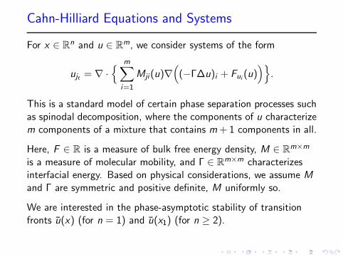
Cahn-Hilliard Equations and Systems
For x ∈ Rn and u ∈ R
m, we consider systems of the form
ujt = ∇ ·
m∑
i=1
Mji(u)∇(
(−Γ∆u)i + Fui (u))
.
This is a standard model of certain phase separation processes suchas spinodal decomposition, where the components of u characterizem components of a mixture that contains m+1 components in all.
Here, F ∈ R is a measure of bulk free energy density, M ∈ Rm×m
is a measure of molecular mobility, and Γ ∈ Rm×m characterizes
interfacial energy. Based on physical considerations, we assume M
and Γ are symmetric and positive definite, M uniformly so.
We are interested in the phase-asymptotic stability of transitionfronts u(x) (for n = 1) and u(x1) (for n ≥ 2).
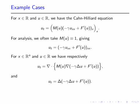
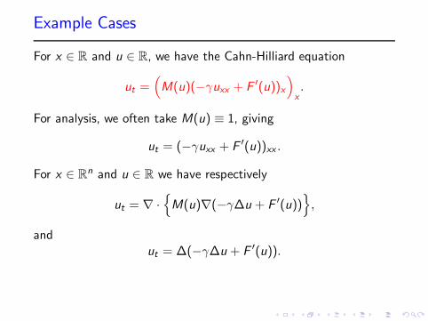
Example Cases
For x ∈ R and u ∈ R, we have the Cahn-Hilliard equation
ut =(
M(u)(−γuxx + F ′(u))x)
x.
For analysis, we often take M(u) ≡ 1, giving
ut = (−γuxx + F ′(u))xx .
For x ∈ Rn and u ∈ R we have respectively
ut = ∇ ·
M(u)∇(−γ∆u + F ′(u))
,
andut = ∆(−γ∆u + F ′(u)).
Example Cases
For x ∈ R and u ∈ R, we have the Cahn-Hilliard equation
ut =(
M(u)(−γuxx + F ′(u))x)
x.
For analysis, we often take M(u) ≡ 1, giving
ut = (−γuxx + F ′(u))xx .
For x ∈ Rn and u ∈ R we have respectively
ut = ∇ ·
M(u)∇(−γ∆u + F ′(u))
,
andut = ∆(−γ∆u + F ′(u)).
Spinodal Decomposition
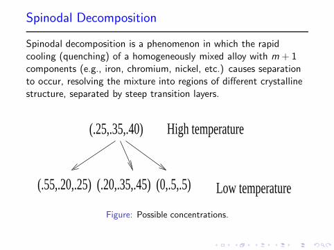
Spinodal decomposition is a phenomenon in which the rapidcooling (quenching) of a homogeneously mixed alloy with m + 1components (e.g., iron, chromium, nickel, etc.) causes separationto occur, resolving the mixture into regions of different crystallinestructure, separated by steep transition layers.
(.25,.35,.40) High temperature
(.55,.20,.25) (.20,.35,.45) (0,.5,.5) Low temperature
Figure: Possible concentrations.


Numerical Simulation
Figure: Numerical simulation for n = 2.

Modeling Spinodal Decomposition
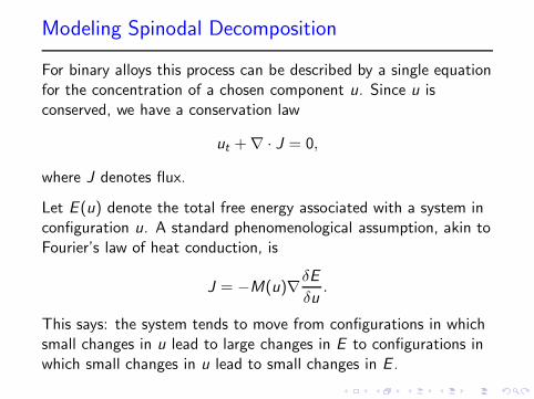
For binary alloys this process can be described by a single equationfor the concentration of a chosen component u. Since u isconserved, we have a conservation law
ut +∇ · J = 0,
where J denotes flux.
Let E (u) denote the total free energy associated with a system inconfiguration u. A standard phenomenological assumption, akin toFourier’s law of heat conduction, is
J = −M(u)∇δE
δu.
This says: the system tends to move from configurations in whichsmall changes in u lead to large changes in E to configurations inwhich small changes in u lead to small changes in E .

Modeling Spinodal Decomposition
For binary alloys this process can be described by a single equationfor the concentration of a chosen component u. Since u isconserved, we have a conservation law
ut +∇ · J = 0,
where J denotes flux.
Let E (u) denote the total free energy associated with a system inconfiguration u. A standard phenomenological assumption, akin toFourier’s law of heat conduction, is
HEAT EQ J = −M(u)∇u HOT → COLD
This says: the system tends to move from configurations in whichsmall changes in u lead to large changes in E to configurations inwhich small changes in u lead to small changes in E .
Modeling Spinodal Decomposition
For binary alloys this process can be described by a single equationfor the concentration of a chosen component u. Since u isconserved, we have a conservation law
ut +∇ · J = 0,
where J denotes flux.
Let E (u) denote the total free energy associated with a system inconfiguration u. A standard phenomenological assumption, akin toFourier’s law of heat conduction, is
J = −M(u)∇δE
δu.
This says: the system tends to move from configurations in whichsmall changes in u lead to large changes in E to configurations inwhich small changes in u lead to small changes in E .

Cahn-Hilliard Energy
In 1958, John W. Cahn and John E. Hilliard suggested the energyE should have the approximate form
E (u) =
ˆ
ΩF (u) +
γ
2|∇u|2dx ,
withδE
δu= F ′(u)− γ∆u.
We expect solutions to evolve toward minimizers of E . Moreprecisely, it’s easy to verify that any solution u(x , t) in anappropriate function class will satisfy
d
dtE (u) = −
ˆ
ΩM(u)
[
(δE
δu)x
]2dx ≤ 0.

Double-well Bulk Free Energy
The Helmholtz free energy is
H = U − TS ⇒ ∂H∂T
= −S .
u u
F(u)
F(u)Temperature Drops
u
u
entropy maximum
1 2
High Temperature
Low Temperature
Figure: Double-well form through quenching.

Intuition about the System
Recall that the energy is
E (u) :=
ˆ
ΩF (u) +
γ
2|∇u|2dx .
One way the system can minimize this is to approach a minimizerof F , but it’s constrained by conservation of mass.
The system can compromise by making transitions from oneminimizer of F to another, but these transitions increase thesecond term in E . The resulting transition fronts are a balancebetween these effects.
Intuition about the System
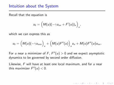
Recall that the equation is
ut =(
M(u)(−γuxx + F ′(u))x)
x,
which we can express this as
ut =(
M(u)(−γuxxx
)
x+
(
M(u)F ′′(u))
xux +M(u)F ′′(u)uxx .
For u near a minimizer of F , F ′′(u) > 0 and we expect asymptoticdynamics to be governed by second order diffusion.
Likewise, F will have at least one local maximum, and for u nearthis maximizer F ′′(u) < 0.

Intuition about the System
Recall that the equation is
ut =(
M(u)(−γuxx + F ′(u))x)
x,
which we can express this as
ut =(
M(u)(−γuxxx
)
x+
(
M(u)F ′′(u))
xux +M(u)F ′′(u)uxx .
For u near a minimizer of F , F ′′(u) > 0 and we expect asymptoticdynamics to be governed by second order diffusion.
Likewise, F will have at least one local maximum, and for u nearthis maximizer F ′′(u) < 0.

Historical Remark on Terminology
The (single) Cahn-Hilliard equation first appeared in John W.Cahn’s paper from 1961, “On spinodal decomposition.”
Cahn-Hilliard systems were first studied by Didier de Fontaine inhis 1967 Northwestern thesis “A computer simulation of theevolution of coherent composition variations in solid solutions,”carried out under the direction of John Hilliard.
de Fontaine explains that Hilliard was never comfortable having hisname on the equation and referred to it himself as “the lastunnumbered equation after equation (18) in Cahn’s 1961 paper.”

Transition Fronts for m = 1
First, since F appears as F ′(u)x , we can replace F with
F (u) = F (u)− au − b,
for any constants a and b. It’s convenient to subtract off asupporting line.
u u1 2
au+b
u u1 2
Figure: Subtraction of the supporting line.

Transition Fronts for m = 1
We say u(x) is a transition front if
0 =(
M(u)(−γuxx + F ′(u))x)
x,
and
limx→−∞
u(x) = u− = u1 (respectively u2)
limx→+∞
u(x) = u+ = u2 (respectively u1)
u1 6= u2
limx→±∞
u′(x) = 0.
Integrating twice, we find
−γuxx + F ′(u) = 0.
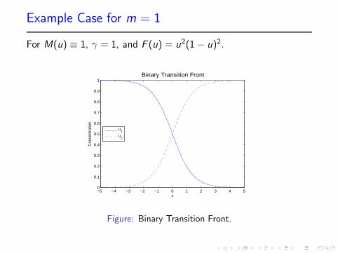
Example Case for m = 1
For M(u) ≡ 1, γ = 1, and F (u) = u2(1− u)2.
−5 −4 −3 −2 −1 0 1 2 3 4 50
0.1
0.2
0.3
0.4
0.5
0.6
0.7
0.8
0.9
1Binary Transition Front
x
Con
cent
ratio
n
u1
u2
Figure: Binary Transition Front.

Asymptotic Behavior
Intuitively, we expect that for fairly general initial conditionsu(x , 0) = u0(x) we will find
limt→∞
u(x , t) = u(x)
for some transition front u(x).
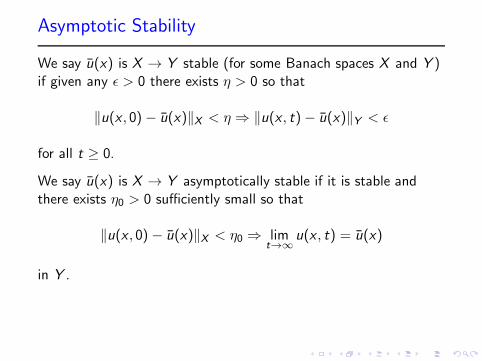
Asymptotic Stability
We say u(x) is X → Y stable (for some Banach spaces X and Y )if given any ǫ > 0 there exists η > 0 so that
‖u(x , 0) − u(x)‖X < η ⇒ ‖u(x , t)− u(x)‖Y < ǫ
for all t ≥ 0.
We say u(x) is X → Y asymptotically stable if it is stable andthere exists η0 > 0 sufficiently small so that
‖u(x , 0) − u(x)‖X < η0 ⇒ limt→∞
u(x , t) = u(x)
in Y .

The Shift
Since concentration is conserved, perturbations of a transitionfront u(x) will not generally approach the front itself, but rather(in the case of stability) a shift of the front.
_
u(x)_
u(x)
δ(t)
x
x
u(0,x)
u(t,x)
Figure: The shifted wave.

Phase-Asymptotic Stability
We define our perturbation as
v(x , t) := u(x + δ(t), t) − u(x).
We say u(x) is X → Y phase-stable if there exists a shift functionδ(t) so that for any ǫ > 0 there exists η > 0 so that
‖v(x , 0)‖X < η ⇒ ‖v(x , t)‖Y < ǫ
for all t ≥ 0.
We say u(x) is X → Y phase-asymptotically stable if u(x) isX → Y phase-stable and there exists a shift function δ(t) and avalue η0 > 0 so that
‖v(x , 0)‖X ≤ η0 ⇒ limt→∞
‖v(x , t)‖Y = 0.

Goal
We establish L1∩L∞ → Lp phase-asymptotic stability for all p > 1.
We obtain L1 ∩ L∞ → L1 phase-stability.

Overview of Recent Results, x ∈ Rn, u ∈ Rm
1. For m = 1, n = 1
J. Bricmont, A. Kupiainen, and J. Taskinen, Comm. PureAppl. Math. 1999
E. Carlen, M. Carvalho, and E. Orlandi, Comm. Math. Phys.2001
H., Comm. Math. Phys. 2007
2. For m = 1, n ≥ 2
T. Korvola, Doctoral Thesis, University of Helsinki 2003
T. Korvola, A. Kupiainen, and J. Taskinen, Comm. PureAppl. Math. 2005
H., Physica D 2007
3. For m ≥ 2, n = 1
H. and B. Kwon, Discrete and Continuous Dynamical SystemsA (spectral analysis) and 2011 Preprints
http://www.math.tamu.edu/˜phoward/mathpubs.html
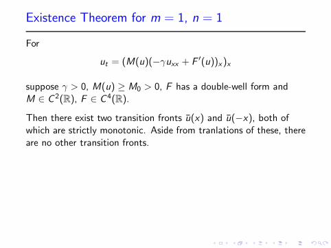
Existence Theorem for m = 1, n = 1
For
ut = (M(u)(−γuxx + F ′(u))x )x
suppose γ > 0, M(u) ≥ M0 > 0, F has a double-well form andM ∈ C 2(R), F ∈ C 4(R).
Then there exist two transition fronts u(x) and u(−x), both ofwhich are strictly monotonic. Aside from tranlations of these, thereare no other transition fronts.
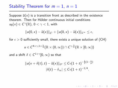
Stability Theorem for m = 1, n = 1
Suppose u(x) is a transition front as described in the existencetheorem. Then for Holder continuous initial conditionsu0(x) ∈ C γ(R), 0 < γ < 1, with
‖u(0, x) − u(x)‖L1 + ‖u(0, x) − u(x)‖L∞ ≤ ǫ,
for ǫ > 0 sufficiently small, there exists a unique solution of (CH)
u ∈C 4+γ,1+ γ
4 (R× (0,∞)) ∩ C γ, γ4 (R× [0,∞))
and a shift δ ∈ C 1+γ[0,∞) so that
‖u(x + δ(t), t)− u(x)‖Lp ≤Cǫ(1 + t)−12(1− 1
p)
|δ(t)− δ∞| ≤Cǫ(1 + t)−1/4.
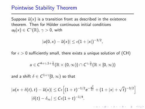
Pointwise Stability Theorem
Suppose u(x) is a transition front as described in the existencetheorem. Then for Holder continuous initial conditionsu0(x) ∈ C γ(R), γ > 0, with
|u(0, x) − u(x)| ≤ ǫ(1 + |x |)−3/2,
for ǫ > 0 sufficiently small, there exists a unique solution of (CH)
u ∈C 4+γ,1+ γ
4 (R× (0,∞)) ∩ C γ, γ4 (R× [0,∞))
and a shift δ ∈ C 1+γ[0,∞) so that
|u(x + δ(t), t)− u(x)| ≤Cǫ[
(1 + t)−1/2e−x2
Lt + (1 + |x |+√t)−3/2
]
|δ(t) − δ∞| ≤Cǫ(1 + t)−1/4.

Linearization
We define our perturbation as
v(x , t) := u(x + δ(t), t) − u(x),
where δ(t) tracks the shift between u(x , t) and u(x). Theperturbation equation is
vt =(
M(u)(−γvxx + F ′′(u)v)x)
x+ δ(t)(ux + vx) + Qx ,
where|Q| ≤ C
[
e−η|x ||v |2 + |v ||vx |+ |v ||vxxx |]
.
This is advantageous because we expect vx and vxxx to decayfaster than v as |x |+ t → ∞. On the other hand, we expect vxand vxxx to blow up respectively like t−1/4 and t−3/4 as t → 0.

The Associated Eigenvalue Problem
The associated linear equation is
vt = Lv :=(
M(u)(−Γvxx + F ′′(u)v)x)
x.
If we look for solutions of the form v(x , t) = eλtφ(x), we obtainthe eigenvalue problem
Lφ = λφ.
The resolvent for this problem is
R(λ; L) := (λI − L)−1,
and we say λ ∈ C is in the resolvent set of L if R(λ; L) is abounded linear operator.
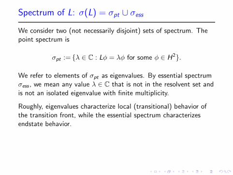
Spectrum of L: σ(L) = σpt ∪ σess
We consider two (not necessarily disjoint) sets of spectrum. Thepoint spectrum is
σpt := λ ∈ C : Lφ = λφ for some φ ∈ H2.
We refer to elements of σpt as eigenvalues. By essential spectrumσess , we mean any value λ ∈ C that is not in the resolvent set andis not an isolated eigenvalue with finite multiplicity.
Roughly, eigenvalues characterize local (transitional) behavior ofthe transition front, while the essential spectrum characterizesendstate behavior.

The Essential Spectrum
The essential spectrum is determined by the asymptotic(x → ±∞) eigenvalue equations
−M(u±)γφxxxx + F ′′(u±)φxx = λφ.
It corresponds with solutions
φ(x) = e iξx ,
so thatλ = −M(u±)γξ
4 − F ′′(u±)ξ2.
By positivity of M and the double-well structure of F ,
σess = (−∞, 0].

The Point Spectrum
First, for λ 6= 0, if φ(x ;λ) solves(
M(u)(−γφxx + F ′′(u)φ)x)
x= λφ,
we can show by integrating both sides that´ +∞−∞ φ(x ;λ)dx = 0.
We set
ϕ(x ;λ) :=
ˆ x
−∞φ(y ;λ)dy ,
so that the integrated eigenvalue problem is
M(u)(−γϕxxx + F ′′(u)ϕx )x = λϕ.
Divide by M(u), multiply by ϕ and integrate to find
−〈ϕx ,−γϕxxx + F ′′(u)ϕx 〉 = λ〈 ϕ
M(u), ϕ〉.
Here, 〈·, ·〉 denotes L2 inner product.

The Eigenvalues λ 6= 0
We can express this last equation as
−〈ϕx ,Hϕx 〉 = λ〈 ϕ
M(u), ϕ〉,
where H is the Schrodinger type operator
H := −γ∂2x + F ′′(u).
NowHu′ = 0,
and u′ has a fixed sign by monotonicity, so by standard secondorder theory H is a non-negative operator. Noting also that H isself-adjoint, we conclude
λ ≤ 0.

The Eigenvalue λ = 0
First, by definition
−γuxx + F ′(u) = 0 ⇒ −γuxxx + F ′′(u)ux = 0
so that φ = ux solves
−γφxx + F ′′(u)φ = 0.
We see that(
M(u)(−γφxx + F ′′(u)φ)x)
= 0,
so that λ = 0 is an eigenvalue with associated eigenfunction ux .
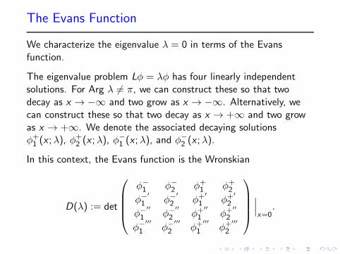
The Evans Function
We characterize the eigenvalue λ = 0 in terms of the Evansfunction.
The eigenvalue problem Lφ = λφ has four linearly independentsolutions. For Arg λ 6= π, we can construct these so that twodecay as x → −∞ and two grow as x → −∞. Alternatively, wecan construct these so that two decay as x → +∞ and two growas x → +∞. We denote the associated decaying solutionsφ+1 (x ;λ), φ
+2 (x ;λ), φ
−1 (x ;λ), and φ−
2 (x ;λ).
In this context, the Evans function is the Wronskian
D(λ) := det
φ−1 φ−
2 φ+1 φ+
2
φ−′
1 φ−′
2 φ+′
1 φ+′
2
φ−′′
1 φ−′′
2 φ+′′
1 φ+′′
2
φ−′′′
1 φ−′′′
2 φ+′′′
1 φ+′′′
2
∣
∣
∣
x=0.
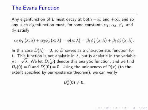
The Evans Function
Any eigenfunction of L must decay at both −∞ and +∞, and soany such eigenfunction must, for some constants α1, α2, β1, andβ2 satisfy
α1φ−1 (x ;λ) + α2φ
−2 (x ;λ) = φ(x ;λ) = β1φ
+1 (x ;λ) + β2φ
+2 (x ;λ).
In this case D(λ) = 0, so D serves as a characteristic function forL. This function is not analytic in λ, but is analytic in the variableρ :=
√λ. We let Da(ρ) denote this analytic function, and we find
Da(0) = 0 and D ′a(0) = 0. Using the uniqueness of u(x) (to the
extent specified by our existence theorem), we can verify
D ′′a (0) 6= 0.

The Classical Semigroup Framework
We can write our full perturbation equation as
vt = Lv + δ(t)(ux + vx) + Qx .
For an initial perturbation v(x , 0), we can express v(x , t) insemigroup formalism as
v(x , t) = eLtv0 +
ˆ t
0eL(t−s)
[
δ(s)u′(y) + δ(s)vy (y , s) + Qy
]
ds,
where by Laplace transform
eLt :=1
2πi
ˆ
ΩeλtR(λ; L)dλ.
Here, Ω denotes a contour in the resolvent set of L, entirely to theright of σ(L), so that arg λ → ±θ as |λ| → ∞ for some θ ∈ (π2 , π).In addition we can move Ω as allowed by Cauchy’s Theorem.
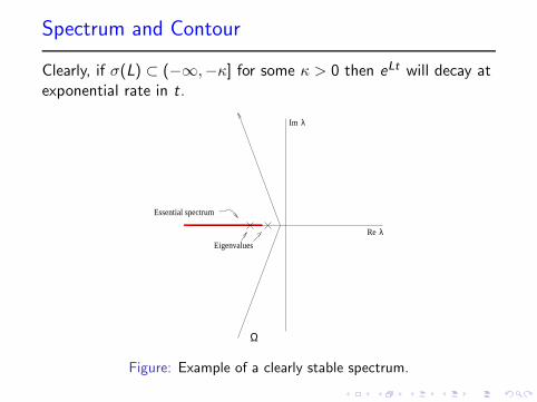
Spectrum and Contour
Clearly, if σ(L) ⊂ (−∞,−κ] for some κ > 0 then eLt will decay atexponential rate in t.
Re λ
Im λ
Essential spectrum
Eigenvalues
Ω
Figure: Example of a clearly stable spectrum.
Spectrum and Contour
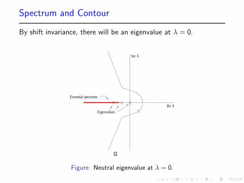
By shift invariance, there will be an eigenvalue at λ = 0.
Ω
Re λ
Im λ
Essential spectrum
Eigenvalues
Figure: Neutral eigenvalue at λ = 0.
Spectrum and Contour
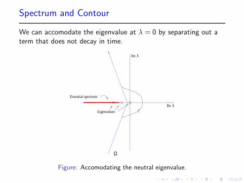
We can accomodate the eigenvalue at λ = 0 by separating out aterm that does not decay in time.
Ω
Re λ
Im λ
Essential spectrum
Eigenvalues
Figure: Accomodating the neutral eigenvalue.

Spectrum and Contour
We can accomodate the eigenvalue at λ = 0 by separating out aterm that does not decay in time.
Ω
Re λ
Im λ
Essential spectrum
Eigenvalues
Figure: Accomodating the neutral eigenvalue.

Spectrum and Contour
We can accomodate the eigenvalue at λ = 0 by separating out aterm that does not decay in time.
Ω
Re λ
Im λ
Essential spectrum
Eigenvalues
Figure: Accomodating the neutral eigenvalue.

Spectrum and Contour
For Cahn-Hilliard systems σess = (−∞, 0].
Re λ
Im λ
Essential spectrum
Eigenvalues
Ω
Figure: Essential spectrum for Cahn-Hilliard systems.

The Pointwise Semigroup Framework
Let G (x , t; y) denote a Green’s function (distribution) for vt = Lv :
Gt = LG
G (x , t; y) = δy (x).
We can express our semigroup operator eLt as
eLt f =
ˆ +∞
−∞G (x , t; y)f (y)dy .
Our expression for v becomes
v(x , t) =
ˆ +∞
−∞G (x , t; y)v0(y)dy + δ(t)u′(x)
+
ˆ t
0
ˆ +∞
−∞G (x , t − s, y)
[
δ(s)v(y , s) + Q]
ydy .

Constructing G
We compute the Laplace transform of G (t → λ), writingLG = Gλ(x ; y), so that
LGλ − λGλ = −δy (x).
Inverting, we find
G (x , t; y) =1
2πi
ˆ
ΩeλtGλ(x ; y)dλ,
where Ω denotes the same contour previously described.

The Choice of Splitting
The main step in the analysis consists of deriving the splitting
G (x , t; y) = u′(x)e(t; y) + G (x , t; y),
where u′(x)e(t; y) is a leading order term associated with λ = 0that does not decay as t → ∞ and G(x , t; y) decays roughly like aheat kernel.
Intuitively, u′(x)e(t; y) captures behavior associated with λ = 0,while G captures behavior associated with essential spectrum.

Choosing the Local Shift
We find (substituting G = u′e + G and integrating by parts)
v(x , t) =
ˆ +∞
−∞G(x , t; y)v0(y)dy + δ(t)u′(x)
−ˆ t
0
ˆ +∞
−∞Gy (x , t − s; y)
[
δ(s)v(y , s) + Q]
dyds
+u′(x)
ˆ +∞
−∞e(t; y)v0(y)dy
−ˆ t
0
ˆ +∞
−∞ey (t − s; y)
[
δ(s)v(y , s) + Q]
dyds
.

Choosing the Local Shift
We find (substituting G = u′e + G and integrating by parts)
v(x , t) =
ˆ +∞
−∞G(x , t; y)v0(y)dy + δ(t)u′(x)
−ˆ t
0
ˆ +∞
−∞Gy (x , t − s; y)
[
δ(s)v(y , s) + Q]
dyds
+u′(x)
ˆ +∞
−∞e(t; y)v0(y)dy
−ˆ t
0
ˆ +∞
−∞ey (t − s; y)
[
δ(s)v(y , s) + Q]
dyds
.
Choosing the Local Shift
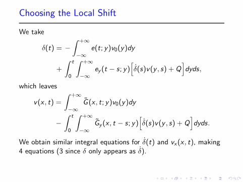
We take
δ(t) = −ˆ +∞
−∞e(t; y)v0(y)dy
+
ˆ t
0
ˆ +∞
−∞ey (t − s; y)
[
δ(s)v(y , s) +Q]
dyds,
which leaves
v(x , t) =
ˆ +∞
−∞G (x , t; y)v0(y)dy
−ˆ t
0
ˆ +∞
−∞Gy(x , t − s; y)
[
δ(s)v(y , s) + Q]
dyds.
We obtain similar integral equations for δ(t) and vx(x , t), making4 equations (3 since δ only appears as δ).

Green’s Function Estimates
Using our spectral information and the structure of our equation,we find for t ≥ 1
e(t; y) = c
ˆ
y√4γM−t
−∞e−z2dz + R(t; y)
|R(t; y)| ≤Ct−1/2e−y2
At ,
and for t ≥ 1 and |x − y | ≥ Kt
|G (x , t; y)| ≤ Ct−1/2e−(x−y)2
At .
Here, c , C , K , η, and A are fixed positive constants dependingonly on the spectrum of L and the structure of the equations.
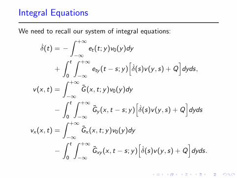
Integral Equations
We need to recall our system of integral equations:
δ(t) = −ˆ +∞
−∞et(t; y)v0(y)dy
+
ˆ t
0
ˆ +∞
−∞ety (t − s; y)
[
δ(s)v(y , s) + Q]
dyds,
v(x , t) =
ˆ +∞
−∞G (x , t; y)v0(y)dy
−ˆ t
0
ˆ +∞
−∞Gy(x , t − s; y)
[
δ(s)v(y , s) + Q]
dyds
vx(x , t) =
ˆ +∞
−∞Gx(x , t; y)v0(y)dy
−ˆ t
0
ˆ +∞
−∞Gxy(x , t − s; y)
[
δ(s)v(y , s) + Q]
dyds.

Linear Stability
Using the estimates we obtain on G , we can verify that∣
∣
∣
ˆ +∞
−∞et(t; y)v0(y)dy
∣
∣
∣≤C (1 + t)−1
∥
∥
∥
ˆ +∞
−∞G (x , t; y)v0(y)dy
∥
∥
∥
Lp≤C (1 + t)
− 12(1− 1
p)
∥
∥
∥
ˆ +∞
−∞Gx(x , t; y)v0(y)dy
∥
∥
∥
Lp≤Ct−1/4(1 + t)−
14 .

Bounding Function ζ(t)
We take these values as preliminary estimates and set
ζ(t) := sup0≤s≤t1≤p≤∞
‖v(·, s)‖Lp (1 + s)12(1− 1
p)
+ ‖vx(·, s)‖Lp s1/4(1 + s)1/4 + |δ(s)|(1 + s)
.
Clearly,
‖v(·, s)‖Lp ≤ ζ(t)(1 + s)−12(1− 1
p)
‖vx(·, s)‖Lp ≤ ζ(t)s−1/4(1 + s)−1/4
|δ(s)| ≤ ζ(t)(1 + s)−1.

Nonlinear Stability
Upon substitution of these bounds into our integral equations, wefind
ζ(t) ≤ C (ǫ+ ζ(t)2).
Here C is a new constant and we recall
‖v(·, 0)‖L1 + ‖v(·, 0)‖L∞ ≤ ǫ.
It’s straightforward to verify that this implies
ζ(t) < 2Cǫ
for all t ≥ 0. This inequality is equivalent with the statement ofour theorem.

Multiple Space Dimensions
For x ∈ Rn the Cahn-Hilliard equation is
ut = ∇ · M(u)∇(−γ∆u + F ′(u)).
In this case, we consider planar transition fronts u(x1). Since u
depends only on x1, planar transition fronts have the samestructure as transition fronts for n = 1. In this case, the shift δ can
depend on the transverse variables x := (x2, x3, . . . , xn), and wedefine our perturbation variable as
v(x , t) := u(x , t)− u(x1 − δ(x , t)).
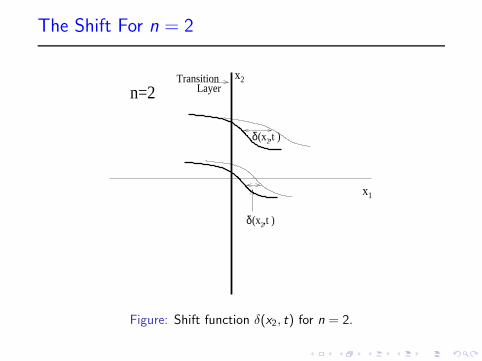
The Shift For n = 2
x
x
1
2Layer
δ
δ
n=2Transition
(x ,t )2
(x ,t )2
Figure: Shift function δ(x2, t) for n = 2.

Linearization
Upon substitution of
v(x , t) := u(x , t)− u(x1 − δ(x , t))
into the Cahn-Hilliard equation we obtain
(∂t − L)v = (∂t − L)(δ(x , t)u′(x1)) +∇ ·Q,
where
Lv =∇ · M(u)∇(−γ∆v + F ′′(u)v)Q =Q(u, δ, v).
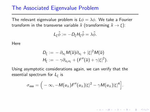
The Associated Eigenvalue Problem
The relevant eigenvalue problem is Lφ = λφ. We take a Fouriertransform in the transverse variable x (transforming x → ξ):
Lξφ := −DξHξφ = λφ.
Here
Dξ := − ∂x1M(u)∂x1 + |ξ|2M(u)
Hξ := − γ∂x1x1 + (F ′′(u) + γ|ξ|2).
Using asymptotic considerations again, we can verify that theessential spectrum for Lξ is
σess =(
−∞,−M(u±)F′′(u±)|ξ|2 − γM(u±)|ξ|4
]
.

The Point Spectrum for ξ 6= 0
For ξ 6= 0 we set ϕ := D−1/2ξ φ (akin to integrating for n = 1) so
thatLξϕ := D
1/2ξ HξD
1/2ξ ϕ = −λϕ.
We can take advantage of the observation that Lξ is self-adjoint toverify that for M0 := minx1∈R M(u(x1))
σpt ⊂ (−∞,−γM0|ξ|4].
Using Evans function techniques, we can show that for |ξ|sufficiently small, the leading (right-most) eigenvalue of Lξ satisfies
λ∗(ξ) = −λ3|ξ|3 +O(|ξ|4),
where
λ3 =
√2γ(M(u−) +M(u+))
|u+ − u−|2ˆ max u−,u+
min u−,u+
√
F (x)− F (u−)dx .

Notes on The Scaling
The cubic scaling for the leading eigenvalue was anticipated by thephysical observation that if S denotes the average pattern sizeduring spinodal decomposition then asymptotically
S ∼ t1/3.
The associated behavior of the leading eigenvalue seems first tohave been recognized by David Jasnow and R. K. P. Zia in 1987.
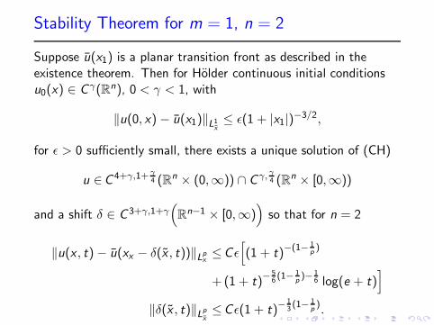
Stability Theorem for m = 1, n = 2
Suppose u(x1) is a planar transition front as described in theexistence theorem. Then for Holder continuous initial conditionsu0(x) ∈ C γ(Rn), 0 < γ < 1, with
‖u(0, x) − u(x1)‖L1x≤ ǫ(1 + |x1|)−3/2,
for ǫ > 0 sufficiently small, there exists a unique solution of (CH)
u ∈C 4+γ,1+ γ
4 (Rn × (0,∞)) ∩ C γ, γ4 (Rn × [0,∞))
and a shift δ ∈ C 3+γ,1+γ(
Rn−1 × [0,∞))
so that for n = 2
‖u(x , t)− u(xx − δ(x , t))‖Lpx ≤Cǫ[
(1 + t)−(1− 1
p)
+(1 + t)− 5
6(1− 1
p)− 1
6 log(e + t)]
‖δ(x , t)‖Lpx≤Cǫ(1 + t)−
13(1− 1
p).

Stability Theorem for m = 1, n ≥ 3
Suppose u(x1) is a planar transition front as described in theexistence theorem. Then for Holder continuous initial conditionsu0(x) ∈ C γ(Rn), 0 < γ < 1, with
‖u(0, x) − u(x1)‖L1 + ‖u(0, x) − u(x1)‖L∞ ≤ ǫ,
for ǫ > 0 sufficiently small, there exists a unique solution of (CH)
u ∈C 4+γ,1+ γ
4 (Rn × (0,∞)) ∩ C γ, γ4 (Rn × [0,∞))
and a shift δ ∈ C 3+γ,1+γ(
Rn−1 × [0,∞)
)
so that for all σ > 0
sufficiently small,
‖u(x , t) − u(x − δ(x , t))‖Lp ≤Cǫ[
(1 + t)−n2(1− 1
p)
+(1 + t)−( n−1
3+ 1
2)(1− 1
p)− 1
6+σ
]
‖δ(x , t)‖Lpx≤Cǫ(1 + t)
− n−13
(1− 1p)+σ
.
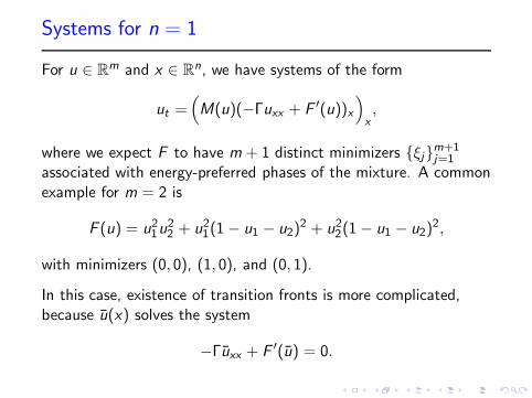
Systems for n = 1
For u ∈ Rm and x ∈ R
n, we have systems of the form
ut =(
M(u)(−Γuxx + F ′(u))x)
x,
where we expect F to have m + 1 distinct minimizers ξjm+1j=1
associated with energy-preferred phases of the mixture. A commonexample for m = 2 is
F (u) = u21u22 + u21(1− u1 − u2)
2 + u22(1− u1 − u2)2,
with minimizers (0, 0), (1, 0), and (0, 1).
In this case, existence of transition fronts is more complicated,because u(x) solves the system
−Γuxx + F ′(u) = 0.

Existence of Transition Fronts
The existence of transition fronts for Cahn-Hilliard systems hasbeen established under quite general conditions by:
N. D. Alikakos, S. I. Betelu, and X. Chen (2006): for m = 2,using complex analysis
N. D. Alikakos and G. Fusco (2008): m ≥ 2, for Γ = I
V. Stefanopoulos (2008): m ≥ 2, for Γ positive definite andsymmetric
In each of these references, the transition fronts arise as minimizersof the associated energy functional
E (u) =
ˆ +∞
−∞F (u) +
1
2〈ux , Γux 〉dx .

Example Case
For m = 2, M(u) ≡ I , Γ = I , and
F (u) = u21u22 + u21(1− u1 − u2)
2 + u22(1− u1 − u2)2.
−10 −8 −6 −4 −2 0 2 4 6 8 100
0.1
0.2
0.3
0.4
0.5
0.6
0.7
0.8
0.9
1Ternary Transition Fronts
x
Con
cent
ratio
n
u1
u2
1−u1−u
2
Figure: Ternary Transition Front.
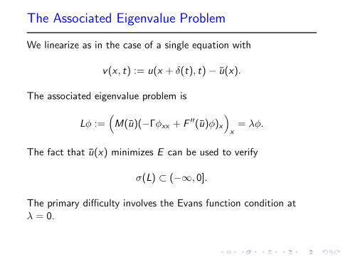
The Associated Eigenvalue Problem
We linearize as in the case of a single equation with
v(x , t) := u(x + δ(t), t) − u(x).
The associated eigenvalue problem is
Lφ :=(
M(u)(−Γφxx + F ′′(u)φ)x)
x= λφ.
The fact that u(x) minimizes E can be used to verify
σ(L) ⊂ (−∞, 0].
The primary difficulty involves the Evans function condition atλ = 0.

The Evans Function
Our eigenvalue problem(
M(u)(−Γφxx + F ′(u)φ)x)
x= λφ
has 2m solutions that decay as x → −∞, φ−j 2mj=1 and 2m
solutions that decay as x → +∞, φ+j 2mj=1. We will set
Φ±j :=
φ±j
φ±′
j
φ±′′
j
φ±′′′
j
, Φ± := (Φ±1 , . . . ,Φ
±2m).
The Evans function is
D(λ) = det(Φ+(0;λ),Φ−(0;λ)).
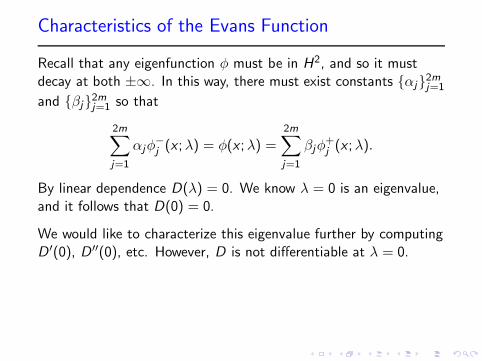
Characteristics of the Evans Function
Recall that any eigenfunction φ must be in H2, and so it mustdecay at both ±∞. In this way, there must exist constants αj2mj=1
and βj2mj=1 so that
2m∑
j=1
αjφ−j (x ;λ) = φ(x ;λ) =
2m∑
j=1
βjφ+j (x ;λ).
By linear dependence D(λ) = 0. We know λ = 0 is an eigenvalue,and it follows that D(0) = 0.
We would like to characterize this eigenvalue further by computingD ′(0), D ′′(0), etc. However, D is not differentiable at λ = 0.

Analyticity of the Evans Function
The solutions φ−j 2mj=1 and φ+
j 2mj=1 have the form
φ−j (x ;λ) = e
µ−2m+j
(λ)x (r−2m+j +O(e−η|x |))
φ+j (x ;λ) = e
µ+j(λ)x (r+j +O(e−η|x |)),
where for j = 1, . . . ,m
µ±j (λ) = −
√
ν±m+1−j +O(|λ|)
µ±m+j(λ) = −
√
λ
β±j
+O(|λ|3/2)
µ±2m+j(λ) =
√
λ
β±m+1−j
+O(|λ|3/2)
µ±3m+j(λ) =
√
ν±j +O(|λ|).
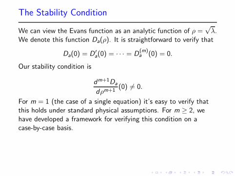
The Stability Condition
We can view the Evans function as an analytic function of ρ =√λ.
We denote this function Da(ρ). It is straightforward to verify that
Da(0) = D ′a(0) = · · · = D
(m)a (0) = 0.
Our stability condition is
dm+1Da
dρm+1(0) 6= 0.
For m = 1 (the case of a single equation) it’s easy to verify thatthis holds under standard physical assumptions. For m ≥ 2, wehave developed a framework for verifying this condition on acase-by-case basis.

Spectral Stability
It’s relatively easy to verify that
σess = (−∞, 0].
If u minimizes the Cahn-Hilliard energy, it’s easy to show that
σpt(L)\0 ⊂ (−∞,−κ]
for some κ > 0. If these conditions both hold, along with ourstability condition
dm+1Da
dρm+1(0) 6= 0.
we say u(x) is spectrally stable.
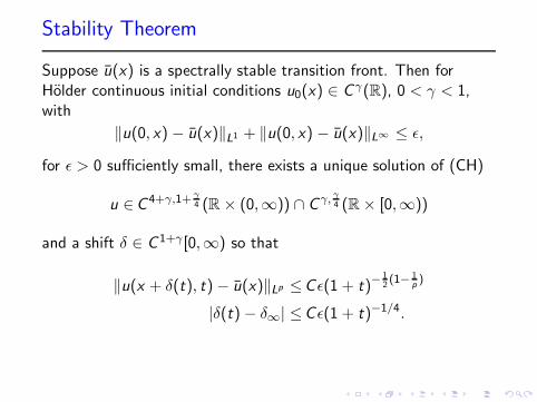
Stability Theorem
Suppose u(x) is a spectrally stable transition front. Then forHolder continuous initial conditions u0(x) ∈ C γ(R), 0 < γ < 1,with
‖u(0, x) − u(x)‖L1 + ‖u(0, x) − u(x)‖L∞ ≤ ǫ,
for ǫ > 0 sufficiently small, there exists a unique solution of (CH)
u ∈C 4+γ,1+ γ
4 (R× (0,∞)) ∩ C γ, γ4 (R× [0,∞))
and a shift δ ∈ C 1+γ[0,∞) so that
‖u(x + δ(t), t)− u(x)‖Lp ≤Cǫ(1 + t)−12(1− 1
p)
|δ(t)− δ∞| ≤Cǫ(1 + t)−1/4.
Further Work
Extension to the case x ∈ Rn, u ∈ R
m, n ≥ 2, m ≥ 2
Periodic and pulse-type stationary solutions for m ≥ 2
Genuinely multidimensional stationary solutions for n ≥ 2
Coarsening dynamics
Navier-Stokes-Cahn-Hilliard systems
The functionalized Cahn-Hilliard equation
ut = ∆
(ǫ2∆−F ′′(u)−ǫη1)(ǫ2∆u−F ′(u))+ǫ(η2−η1)F
′(u)


![The Maslov index and spectral counts for …phoward/papers/hjk1.pdfMaslov index is provided in Section 2, and a thorough discussion can be found in [8]. As a starting point, we de](https://static.fdocuments.us/doc/165x107/5fb2b563d606a858bc20cfc5/the-maslov-index-and-spectral-counts-for-phowardpapershjk1pdf-maslov-index-is.jpg)