Phase 1 Statistical Analysis Plan - clinicaltrials.gov · on race, sex, age, diagnosis (stroke...

Phase 1

Statistical Analysis Plan

May 15 2018

Phase 1 Statistical Analysis Plan

STUDY TITLE: Comprehensive Post-Acute Stroke Services (COMPASS) Study

COMMUNICATING PI: Pamela Duncan, PhD

JOINT PIs: Cheryl Bushnell, MD; Wayne Rosamond, PhD

FUNDING AGENCY: Patient-Centered Outcomes Research Institute

PROGRAM AWARD NUMBER: PCS-1403-14532

CLINICAL TRIALS NUMBER: NCT02588664

AUTHOR: Matthew A. Psioda, PhD

ANALYSIS PLAN VERSION: 1.0

DATE: May 15, 2018

Phase I Statistical Analysis Plan

15 May 2018

Page i

SIGNATURE PAGE

Name Role Signature Date

Pamela Duncan Principal

Investigator 5/16/2018

Cheryl Bushnell Co-Principal

Investigator

5/17/2018

Wayne

Rosamond

Co-Principal

Investigator

5/17/2018

Matthew Psioda

Lead

Statistician; Co-

Investigator

5/15/2018

Ralph B.

D’Agostino Jr.

Sn. Statistician;

Co-Investigator

5/23/2018


15 May 2018

Page ii

Table of Contents

1 List of Abbreviations ............................................................................................................... 1

2 Introduction ............................................................................................................................. 2

3 Study Design............................................................................................................................ 2

3.1 Study Population .................................................................................................................. 2

3.2 Randomization ..................................................................................................................... 2

3.3 Sample Size Calculations & Statistical Power..................................................................... 2

4 Primary and Secondary Objectives.......................................................................................... 4

4.1 Primary Objective ................................................................................................................ 4

4.2 Secondary Objectives........................................................................................................... 4

5 Primary and Secondary Endpoints .......................................................................................... 4

5.1 Primary Endpoint – Stroke Impact Scale 16 ........................................................................ 4

5.2 Secondary Endpoints Based on 90-day Surveys .................................................................. 5

5.2.1 Modified Caregiver Strain Index .............................................................................. 5

5.2.2 Self-Reported General Health ................................................................................... 6

5.2.3 Secondary Prevention – Home Blood Pressure Monitoring ..................................... 6

5.2.4 Self-Reported Blood Pressure .................................................................................. 6

5.2.5 Cognition – Montreal Cognitive Assessment (MoCA) 5-Minute Protocol .............. 6

5.2.6 Depression................................................................................................................. 6

5.2.7 Physical Activity ....................................................................................................... 7

5.2.8 Fatigue....................................................................................................................... 7

5.2.9 Falls ........................................................................................................................... 8

5.2.10 Disability and Dependence – Modified Rankin Scale .............................................. 8

5.2.11 Four-Item Morisky Green Levine Scale (MGLS-4) ................................................. 8

5.2.12 Satisfaction with Care ............................................................................................... 8

6 Analysis Populations ............................................................................................................... 9

6.1 Intent-to-Treat Analysis ....................................................................................................... 9

6.2 Per-Protocol Intervention Analysis ...................................................................................... 9

7 Intent-to-Treat Analysis of the Primary Endpoint ................................................................. 10

7.1 Primary Outcome Ascertainment and Bias Correction through IPW ................................ 10

7.2 Multiple Imputation to Address Covariate Missingness .................................................... 11


15 May 2018

Page iii

7.3 Assessment of a Treatment by Diagnosis Interaction ........................................................ 11

7.4 Supplemental/Sensitivity ITT Analyses for the Primary Endpoint ................................... 11

7.4.1 Possible Ceiling/Floor Effect & Other Violations of LMM Assumptions ............. 11

7.4.2 Primary Endpoint Truncation by Death .................................................................. 12

7.5 Per-Protocol Analysis of the Primary Endpoint................................................................. 12

7.5.1 Correction for Selection Bias Due to Missing Outcomes ....................................... 15

7.5.2 Missing Covariate Data........................................................................................... 15

8 Analysis of Secondary Endpoints Based on 90-day Survey Data ......................................... 15

8.1 Analysis of Modified Caregiver Strain Index Endpoint .................................................... 15

8.2 Analysis of Other Patient-Reported Secondary Endpoints ................................................ 15

9 Subgroup Analyses ................................................................................................................ 16

Bibliography ................................................................................................................................. 17


15 May 2018

Page 1

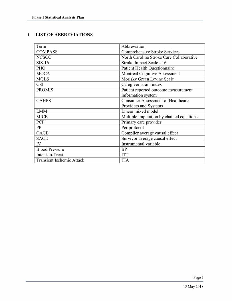
1 LIST OF ABBREVIATIONS

Term Abbreviation

COMPASS Comprehensive Stroke Services

NCSCC North Carolina Stroke Care Collaborative

SIS-16 Stroke Impact Scale - 16

PHQ Patient Health Questionnaire

MOCA Montreal Cognitive Assessment

MGLS Morisky Green Levine Scale

CSI Caregiver strain index

PROMIS Patient reported outcome measurement

information system

CAHPS Consumer Assessment of Healthcare

Providers and Systems

LMM Linear mixed model

MICE Multiple imputation by chained equations

PCP Primary care provider

PP Per protocol

CACE Complier average causal effect

SACE Survivor average causal effect

IV Instrumental variable

Blood Pressure BP

Intent-to-Treat ITT

Transient Ischemic Attack TIA


15 May 2018

Page 2

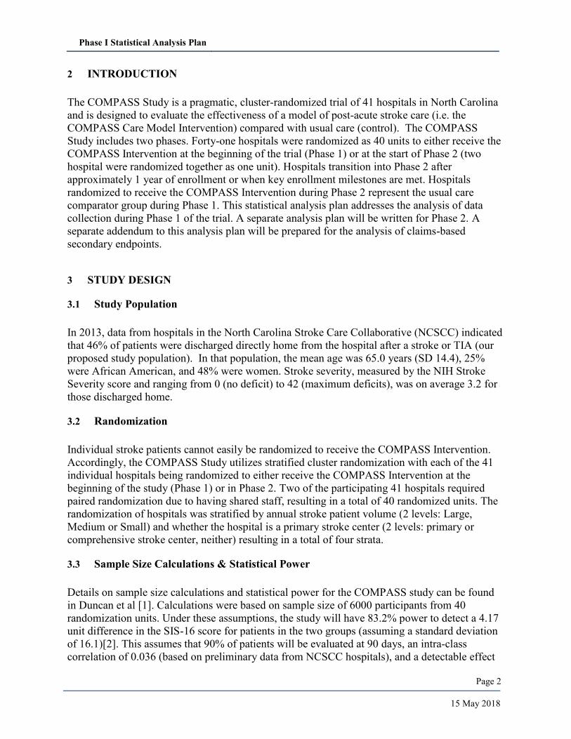
2 INTRODUCTION

The COMPASS Study is a pragmatic, cluster-randomized trial of 41 hospitals in North Carolina

and is designed to evaluate the effectiveness of a model of post-acute stroke care (i.e. the

COMPASS Care Model Intervention) compared with usual care (control). The COMPASS

Study includes two phases. Forty-one hospitals were randomized as 40 units to either receive the

COMPASS Intervention at the beginning of the trial (Phase 1) or at the start of Phase 2 (two

hospital were randomized together as one unit). Hospitals transition into Phase 2 after

approximately 1 year of enrollment or when key enrollment milestones are met. Hospitals

randomized to receive the COMPASS Intervention during Phase 2 represent the usual care

comparator group during Phase 1. This statistical analysis plan addresses the analysis of data

collection during Phase 1 of the trial. A separate analysis plan will be written for Phase 2. A

separate addendum to this analysis plan will be prepared for the analysis of claims-based

secondary endpoints.

3 STUDY DESIGN

3.1 Study Population

In 2013, data from hospitals in the North Carolina Stroke Care Collaborative (NCSCC) indicated

that 46% of patients were discharged directly home from the hospital after a stroke or TIA (our

proposed study population). In that population, the mean age was 65.0 years (SD 14.4), 25%

were African American, and 48% were women. Stroke severity, measured by the NIH Stroke

Severity score and ranging from 0 (no deficit) to 42 (maximum deficits), was on average 3.2 for

those discharged home.

3.2 Randomization

Individual stroke patients cannot easily be randomized to receive the COMPASS Intervention.

Accordingly, the COMPASS Study utilizes stratified cluster randomization with each of the 41

individual hospitals being randomized to either receive the COMPASS Intervention at the

beginning of the study (Phase 1) or in Phase 2. Two of the participating 41 hospitals required

paired randomization due to having shared staff, resulting in a total of 40 randomized units. The

randomization of hospitals was stratified by annual stroke patient volume (2 levels: Large,

Medium or Small) and whether the hospital is a primary stroke center (2 levels: primary or

comprehensive stroke center, neither) resulting in a total of four strata.

3.3 Sample Size Calculations & Statistical Power

Details on sample size calculations and statistical power for the COMPASS study can be found

in Duncan et al [1]. Calculations were based on sample size of 6000 participants from 40

randomization units. Under these assumptions, the study will have 83.2% power to detect a 4.17

unit difference in the SIS-16 score for patients in the two groups (assuming a standard deviation

of 16.1)[2]. This assumes that 90% of patients will be evaluated at 90 days, an intra-class

correlation of 0.036 (based on preliminary data from NCSCC hospitals), and a detectable effect


15 May 2018

Page 3

of 0.192 times the within-group standard deviation. The COMPASS Study was also designed to

detect differences within subgroups of interest that comprise at least 20% of the overall sample

(e.g., stroke subtype, severity, insurance status, geographic area of residence, race, and gender).

Based on preliminary data during the first year of the COMPASS study, it became apparent that

approximately 60%-65% of participants would have an ascertained outcome and that the

distribution of sample sizes across the clusters was more heterogeneous that originally expected.

Therefore, the data analysis core re-estimated the statistical power based on the following revised

assumptions:

1. Final enrollment for each hospital could be accurately predicted based on the hospital’s

average enrollment rate at that point in the trial.

2. The number of hospitals enrolling participants would be 39.

3. The total number of participants enrolled would be approximately 5973.

4. Response rate for the primary outcome would be approximately 65% and would be

consistent across hospitals leading to an effective sample size of approximately 3882

participants.

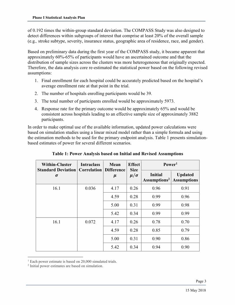
In order to make optimal use of the available information, updated power calculations were

based on simulation studies using a linear mixed model rather than a simple formula and using

the estimation methods to be used for the primary endpoint analysis. Table 1 presents simulation-

based estimates of power for several different scenarios.

Table 1: Power Analysis based on Initial and Revised Assumptions

Within-Cluster

Standard Deviation

𝝈

Intraclass

Correlation

Mean

Difference

𝝁

Effect

Size

𝝁 𝝈⁄

Power1

Initial

Assumptions2

Updated

Assumptions

16.1 0.036 4.17 0.26 0.96 0.91

4.59 0.28 0.99 0.96

5.00 0.31 0.99 0.98

5.42 0.34 0.99 0.99

16.1

0.072

4.17 0.26 0.78 0.70

4.59 0.28 0.85 0.79

5.00 0.31 0.90 0.86

5.42 0.34 0.94 0.90

1 Each power estimate is based on 20,000 simulated trials. 2 Initial power estimates are based on simulation.


15 May 2018

Page 4

4 PRIMARY AND SECONDARY OBJECTIVES

4.1 Primary Objective

The primary objective of the COMPASS Study is to evaluate the comparative effectiveness of

the COMPASS Intervention compared to usual care with respect to improving stroke survivor

functional status (measured by the Stroke Impact Scale) at 90 days post-discharge.

4.2 Secondary Objectives

The key secondary objectives of the COMPASS Study are as follows:

1. Evaluate comparative effectiveness of the COMPASS Intervention with respect to

reducing caregiver strain (measured by the Modified Caregiver Strain Index) at 90 days

post-discharge.

2. Using responses from the 90-day patient survey, evaluate whether the COMPASS

Intervention improves general health, global disability, physical activity, depression

(PHQ2), cognition (Mini MOCA), medication adherence (MGLS-4), management of

blood pressure, incidence of falls, incidence of fatigue, and satisfaction with care.

3. Evaluate the effectiveness of the COMPASS Intervention in key patient subgroups based

on race, sex, age, diagnosis (stroke versus TIA), stroke severity, and type of health

insurance.

4. Endpoints to be addressed in SAP Addendum: Using claims data from multiple payer

sources up to 12 months after stroke hospitalization, evaluate comparative effectiveness

of the COMPASS Intervention with respect to the following outcomes:

a. all-cause hospital readmissions at 30 days, 90 days, and 1 year post-discharge

b. all-cause mortality up to 1 year post-discharge

c. healthcare utilization (emergency department visits, admissions to skilled nursing

facilities/inpatient rehabilitation facilities) up to 1 year post-discharge

d. use of transitional care management billing codes

5 PRIMARY AND SECONDARY ENDPOINTS

5.1 Primary Endpoint – Stroke Impact Scale 16

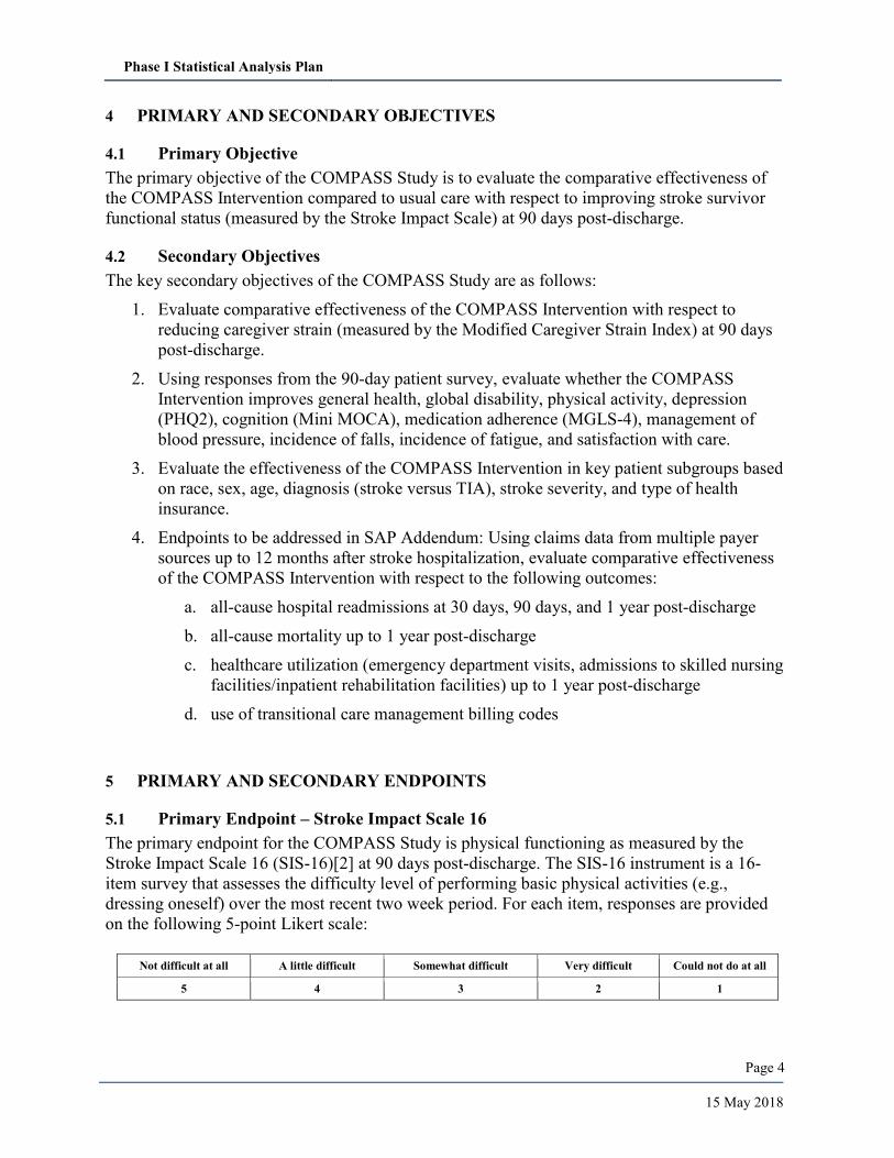
The primary endpoint for the COMPASS Study is physical functioning as measured by the

Stroke Impact Scale 16 (SIS-16)[2] at 90 days post-discharge. The SIS-16 instrument is a 16-

item survey that assesses the difficulty level of performing basic physical activities (e.g.,

dressing oneself) over the most recent two week period. For each item, responses are provided

on the following 5-point Likert scale:

Not difficult at all A little difficult Somewhat difficult Very difficult Could not do at all

5 4 3 2 1


15 May 2018

Page 5

A raw score is obtained for each participant by summing individual item scores. For participants

who complete all 16 items, the maximum possible raw score is 80 and the minimum possible raw

score is 16. A survey is considered scoreable if a participant answers at least 12 of the 16 items.

Standardized scores are computed for each valid raw score using the following formula:

analysis score = raw score−𝑛

5𝑛−𝑛× 100,

where 𝑛 is the number of items answered by the participant. Thus, the standardized scores for all

participants will have a possible range from 0 to 100 with larger scores corresponding to

outcomes that are more favorable.

Ninety-day patient outcomes were assessed through telephone interviews by trained and blinded

interviewers using Computer Assisted Telephone Interviewing (CATI) software. For

participants who could not be reached by phone (e.g., invalid phone number, 10 call attempts

with no answer), an abbreviated survey was subsequently sent by mail to the participant address

on record. This mailed survey included only the SIS-16, self-rated health, and last measured

blood pressure. In the rare event that a participant completed a telephone and mailed survey, the

SIS-16 from the telephone survey was selected as the participant’s SIS16 outcome unless fewer

than 12 items were completed. In such cases, the SIS-16 outcome from the mailed survey was

selected. Although the 90-day survey would ideally be completed approximately 90 days after

discharge, all scoreable surveys will be included in the primary analysis regardless of the precise

time of completion.

5.2 Secondary Endpoints Based on 90-day Surveys

5.2.1 Modified Caregiver Strain Index

The Modified Caregiver Strain Index (CSI) can be used to assess caregiver strain with familial

caregivers [3]. This tool measures strain that caregivers may experience in the following

domains: Financial, Physical, Psychological, Social, and Personal. To complete the survey,

caregivers respond to 13 statements regarding the care they provide. Example statements include

“My sleep is disturbed (For example: the person I care for is in and out of bed or wanders around

at night)” and “Caregiving is inconvenient (For example: helping takes so much time or it’s a

long drive over to help)”. Responses to each of the 13 statements are scored according to the

following criteria:

2 = Yes, on a regular basis

1 = Yes, sometimes

0 = No

For participants who complete all 13 items, the maximum possible raw score is 26 and the

minimum possible raw score is 0. A survey is considered scoreable if a caregiver answers at least

10 of the 13 items. Standardized scores are computed for each valid raw score using the

following formula:

analysis score = actual raw score

2n× 100,


participants will have a possible range from 0 to 100 with larger scores indicating more caregiver

burden.


15 May 2018

Page 6

The caregiver survey is mailed to all eligible caregivers on record approximately 95 days after

patient discharge. Not all participants indicated having a caregiver. Caregivers of patients who

died prior to 90 days, are residing in a facility, or who withdraw from the study are not mailed a

survey.

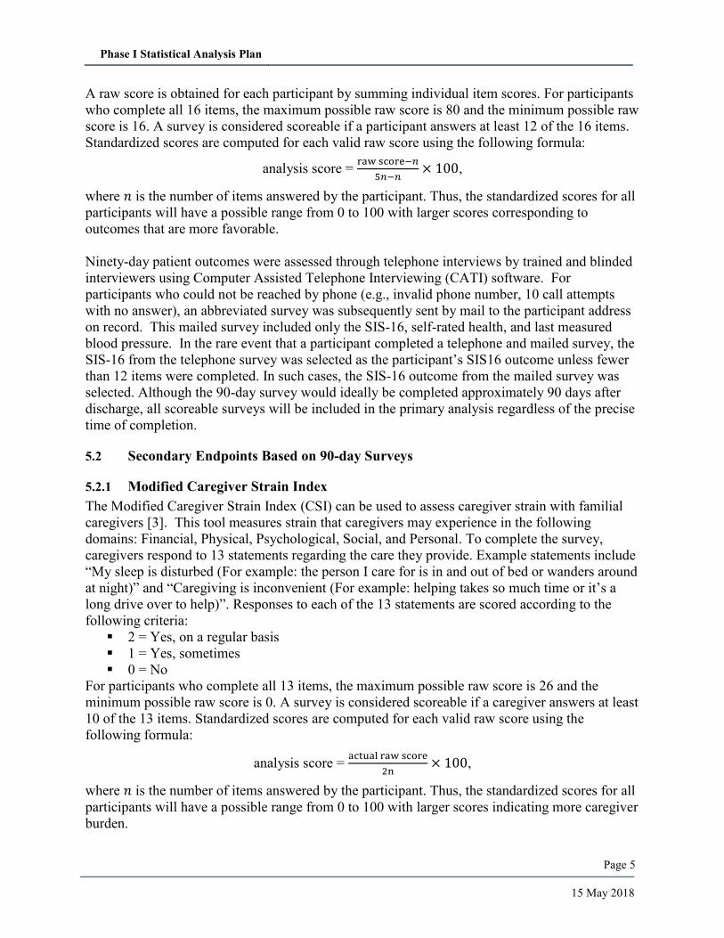
5.2.2 Self-Reported General Health

Participants are asked to self-rate their general health since their stroke or TIA using the

following 5-point Likert scale:

Compared to others your age, how would you rate

your health since your stroke using a scale between

1 and 5 with 1 being “poor” and 5 being

“excellent?”

Poor Fair Good Very

Good Excellent

Self-reported general health will be analyzed as a continuous variable. Following [4], these

responses will be transformed for analysis according to the following criteria:

Excellent = 95

Very Good = 90

Good = 80

Fair = 30

Poor = 15

5.2.3 Secondary Prevention – Home Blood Pressure Monitoring

Participants are asked whether they monitor their blood pressure at home (yes or no) and, if they

answer in the affirmative, how frequently (daily, weekly, and monthly). Home blood pressure

monitoring will be analyzed as a dichotomous endpoint (monitoring with any frequency versus

no monitoring).

5.2.4 Self-Reported Blood Pressure

Self-reported systolic and diastolic BP will each be analyzed as a continuous endpoint. In

addition, self-reported systolic and diastolic BP will be used to create a dichotomous

hypertension endpoint (systolic BP >= 140 versus systolic BP < 140).

5.2.5 Cognition – Montreal Cognitive Assessment (MoCA) 5-Minute Protocol

The MoCA 5-minute protocol is a brief cognitive protocol for screening for vascular cognitive

impairment [5], [6]. The tool includes 4 items from the full MoCA and examines attention,

verbal learning and memory, executive functions/language, and orientation. Each of the four

items are scored separately and the scores are summed to obtain a total score that falls between 0

and 30 for analysis as a continuous variable.

5.2.6 Depression

The PHQ-2 is a 2-item questionnaire that inquires about the frequency of depressed mood and

anhedonia over the past 2 weeks [7]. The first question asks how often the participant had little

interest or pleasure in doing things and the second asks how often the participant felt down,


15 May 2018

Page 7

depressed, or hopeless. Each of the two questions are answered using a Likert scale with the

following scoring rubric:

0 = Not at all

1 = Several days

2 = More than half the days

3 = Nearly every day

The total score is the sum of the scores for the two questions and ranges from 0-6. For analysis,

following standard screening criteria [7], the total score will be dichotomized (total score >= 3

versus total score <3).

5.2.7 Physical Activity

Physical activity is assessed in several ways. Patients are asked whether they walked

continuously for at least 10 minutes on any of the last seven days, how many of those days they

walked continuously for at least 10 minutes and how many minutes they walked, on average,

each day. The physical activity endpoint will be self-reported total number of minutes walked

during the past seven days. Total number of minutes walked will be log-transformed prior to

analysis.

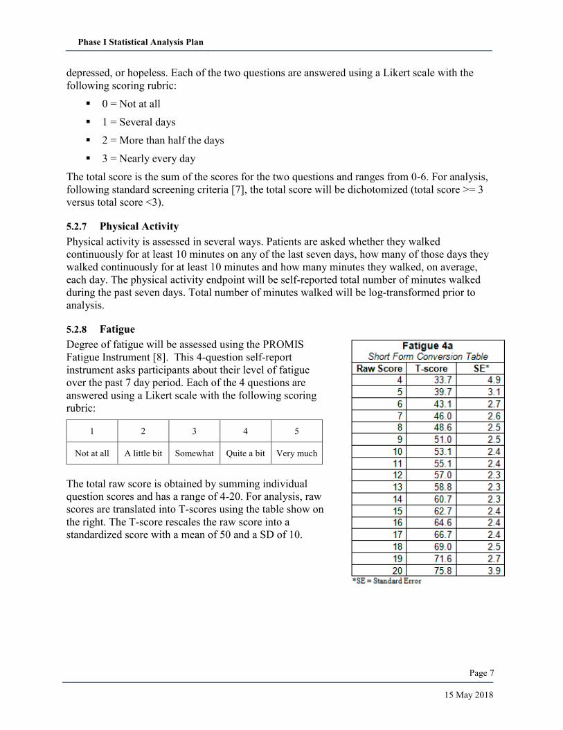
5.2.8 Fatigue

Degree of fatigue will be assessed using the PROMIS

Fatigue Instrument [8]. This 4-question self-report

instrument asks participants about their level of fatigue

over the past 7 day period. Each of the 4 questions are

answered using a Likert scale with the following scoring

rubric:

1 2 3 4 5

Not at all A little bit Somewhat Quite a bit Very much

The total raw score is obtained by summing individual

question scores and has a range of 4-20. For analysis, raw

scores are translated into T-scores using the table show on

the right. The T-score rescales the raw score into a

standardized score with a mean of 50 and a SD of 10.


15 May 2018

Page 8

5.2.9 Falls

Participants are asked whether they have fallen (yes versus no) since hospital discharge, whether

or not the fall resulted in a doctor/emergency room visit, whether they have fallen multiple times

since discharge, and how many times they have fallen since discharge. Analysis of falls will be

based on incidence of any fall since hospital discharge (no falls versus at least one fall).

5.2.10 Disability and Dependence – Modified Rankin Scale

The Modified Rankin Scale measures the degree of disability or dependence in daily activities

for people who have suffered a stroke [9]. The scale ranges from 0-6 according to the following

criteria:

0 - No symptoms

1 - No significant disability. Able to carry out all usual activities, despite some symptoms.

2 - Slight disability. Able to look after own affairs without assistance, but unable to carry out

all previous activities.

3 - Moderate disability. Requires some help, but able to walk unassisted.

4 - Moderately severe disability. Unable to attend to own bodily needs without assistance,

and unable to walk unassisted.

5 - Severe disability. Requires constant nursing care and attention, bedridden, incontinent

6 - Dead

Since 90-day survey respondents are alive at the time of survey completion, survey responses

will fall between 0 and 5. A value of 6 will be assigned for all participants who are confirmed to

have died prior to completion of the 90-days outcomes protocol based on the North Carolina

state mortality database.

5.2.11 Four-Item Morisky Green Levine Scale (MGLS-4)

The Morisky Green Levine Scale (MGLS-4) is a generic self-reported, medication-taking

behavior scale, validated for hypertension, but used for a wide variety of medical conditions. The

instrument consists of four items with yes/no response options [10] which are scored as 1/0,

respectively. The items are summed to obtain a total score that is classified into the following

groups:

High adherence – total score = 0

Medium adherence – total score = 1 or 2

Low adherence – total score = 3 or 4

Medication adherence will be analyzed as a three category ordinal variable.

5.2.12 Satisfaction with Care

Participant satisfaction with care will be assessed using the Consumer Assessment of Health

Plans and Services Clinician and Group Survey (CG-CAHPS, version 3.0). This instrument

includes 6 questions that ask about how often the patient’s doctors explained concepts in a way

that was easy to understand, listened carefully, knew important medical history, showed respect

for what the patient had to say, spent sufficient time with the patient, and talked about all of the


15 May 2018

Page 9

patient’s prescription medications. The individual questions are answered using a Likert scale

with the following scoring rubric:

1 = Never

2 = Sometimes

3 = Usually

4 = Always

A total raw score is obtained by summing the individual question scores and has a range of 4-24

if all questions are answered. Standardized scores will be computed for each valid raw score

using the following formula:

analysis score = actual raw score

4n−n× 100,


participants will have a possible range from 0 to 100 with greater scores indicating more

satisfaction with care.

6 ANALYSIS POPULATIONS

In the COMPASS Study, data are collected during the initial hospital stay, follow-up clinical

assessments for the intervention arm (by telephone and at an in-person clinic visit), during a

telephone survey, and potentially by mailed survey. Use of the data from different sources are

subject to different patient consent requirements per the study IRB. The analysis populations

defined below specify broad collections of patients that will be used for analyses. Particular

analyses may be further restricted based on specific consent requirements for the data being

analyzed.

6.1 Intent-to-Treat Analysis

The Intent-to-Treat (ITT) population will include all patients who are enrolled in the study.

Participants re-enrolled for subsequent stroke or TIA events are not included in the ITT

population. This population will be used for the analysis of primary and secondary endpoints

unless otherwise stated. For all intent-to-treat analyses, participants in the intervention arm of the

study will be analyzed as having received the intervention regardless of which components, if

any, they actually received. Intent-to-treat analyses will compare outcomes for intervention

patients to those from usual care patients.

6.2 Per-Protocol Intervention Analysis

Participants in the intervention arm of the study will be subdivided into two categories: (1)

participants receiving an eCare plan at the COMPASS clinic visit within 30 calendar days of

hospital discharge, and (2) participants not meeting the criteria in (1). Participants meeting

criteria (1) are referred to as Per-Protocol Intervention (PPI) participants and those meeting

criteria (2) are referred to as non-PPI participants.

The goal of the Per-Protocol (PP) analysis is to estimate the complier average causal effect

(CACE) of the COMPASS intervention compared to usual care. That is, the effect of the


15 May 2018

Page 10

COMPASS intervention compared to usual care among those patients who would comply with

treatment recommendations (e.g., attend the clinic visit to receive an eCare Plan for intervention

arm participants). This is done through the framework of compliance principle stratification [11].

Formal details of the analysis strategy are given in Section 7.5.

7 INTENT-TO-TREAT ANALYSIS OF THE PRIMARY ENDPOINT

As standardized SIS-16 scores are semi-continuous in nature, the primary analysis will be based

on a weighted linear mixed model (LMM) that includes a hospital-specific random effect (i.e.,

random intercept), a four-level stratification variable (see Section 3.2), a treatment effect, a

patient-level effect for diagnosis type (stroke versus TIA) and other patient-level potential

confounders (or surrogates thereof) for which there is a meaningful imbalance between the two

study arms (see Section 7.4.3).

The case-weights used for the LMM will be case-specific inverse probabilities for ascertainment

of the primary outcome. This approach is commonly referred to as inverse probability weighting

(IPW) or simply weighting using propensity scores. Estimation of the case-specific propensities

is described in Section 7.1. Estimation of the weighted LMM will be performed using restricted

maximum likelihood methods. Degrees of freedom for tests of the treatment effect will be

estimated using the method of Kenward and Roger [12]. The pre-planned adjustment for

diagnosis type is justified by the fact that TIA patients (on average) are hypothesized to have

better functional outcomes than stroke patients and by including this covariate, the analysis

should have added precision and increased power.

Since the COMPASS Study randomizes hospitals and not patients, the randomization does not

ensure balance with respect to patient characteristics across the two study arms. As a result,

statistical analyses that do not adjust for potential confounders may be biased. In order to assure

that analysis of the primary endpoint is robust, we will consider adjustments for potential

confounders that are both meaningfully imbalanced across the two study arms and potentially

casually related to the primary outcome. Candidate confounders include the following: race

(white versus non-white), age, diagnosis (stroke versus TIA), NIH Stroke Scale Score (NIHSS),

history of stroke or TIA, presence of multiple comorbidities, ability to ambulate prior to

admission, ability to ambulate at discharge, having a primary care provider (PCP), whether the

patient has medical insurance, and number of and type of therapy referrals prior to discharge.

7.1 Primary Outcome Ascertainment and Bias Correction through IPW

Based on preliminary data from the COMPASS Study, we expect that primary outcome

ascertainment will occur for approximately 60%-65% of patients and >=60% of patients in each

study arm. Due to the significant number of missing primary outcomes, a complete case analysis

could be biased. Accordingly, the primary analysis will account for primary outcome

nonresponse by weighting cases with an observed outcome based on the inverse of their

propensity for outcome ascertainment as estimated using a logistic regression model. If the data

suggest a cluster-specific effect on outcome ascertainment, we will consider conditional logistic

regression which has been shown to avoid bias due to cluster-specific nonignorable nonresponse

[13].


15 May 2018

Page 11

Propensities will be estimated separately for each study arm using common set of covariate

predictors. The set of predictors will be selected prior to any unmasked analyses of any primary

or secondary endpoint data. Candidate predictors include the following: race (white versus non-

white), age, diagnosis (stroke versus TIA), NIHSS, history of stroke or TIA, presence of multiple

comorbidities, ability to ambulate prior to admission, ability to ambulate at discharge, having a

PCP, whether the patient has medical insurance, and number and type of therapy referrals prior

to discharge.

Patients who die prior to the date of the 90-day survey will be excluded from the analyses that

estimates case-specific propensities and from the actual primary analysis. Thus, the primary

analysis will effectively be performed conditional on 90-day survival.

7.2 Multiple Imputation to Address Covariate Missingness

Preliminary data from the COMPASS Study suggest that several important baseline

characteristics will be missing for 10% to 30% of patients. These characteristics include NIHSS

(approximately 15%) and ambulatory status at discharge (22%). We will use multiple imputation

by chained equations (MICE) [14] to impute missing NIHSS, ambulatory status at discharge, and

other potential confounders as necessary. Primary and secondary endpoint analyses will be based

on 100 imputed datasets. For each imputed dataset, the IPW analysis procedure described above

will be performed and the parameter estimates will be combined across imputed datasets using

standard techniques [15]. Thus, the primary ITT analysis can be viewed as a combination of

multiple imputation to address covariate missingness and inverse probability weighting to

address failed outcome ascertainment.

7.3 Assessment of a Treatment by Diagnosis Interaction

While we a priori expect for both stroke and TIA patients to benefit comparably from the

COMPASS Intervention, it is plausible that the benefit to TIA patients could be less than that for

stroke patients owing to the comparatively less severe nature of TIAs. To that end, we will assess

the degree to which the data support the assumption of a homogeneous intervention effect for

both stroke and TIA patients as a first step in the primary analysis. This will be done by fitting an

augmented weighted LMM that includes a treatment by diagnosis type interaction and by

formally testing the interaction at significance level 0.10. If the interaction is not statistically

significant at level 0.10, the primary ITT analysis will be performed at level 0.05 as described

above. However, if the interaction is significant at level 0.10 the primary ITT analysis will be

performed by assessing the impact of the COMPASS Intervention on both stroke and TIA

patients separately from a single model with the familywise type I error rate controlled using the

Hommel’s method [16].

7.4 Supplemental/Sensitivity ITT Analyses for the Primary Endpoint

7.4.1 Possible Ceiling/Floor Effect & Other Violations of LMM Assumptions

Because of the bounded nature of standardized SIS-16 scores and the significant proportion of

TIA patients enrolled in the COMPASS study (approximation 35%), there is a potential for a

ceiling effect whereby a non-negligible proportion of the patient population experience the most

extreme outcomes supported by the instrument. In these cases, the assumption of normality for

the weighted LMM is not tenable though the linear model in known to provide robust inference


15 May 2018

Page 12

in many cases. If 15% or more of cases have a SIS-16 outcome equal to the ceiling of the

instrument, we will perform a secondary analysis based on a categorical SIS-16 outcome with

categories defined using the quintiles of the observed SIS-16 scores. A weighted ordinal logistic

regression model will be used for this analysis. More generally, we will use standard diagnostic

tools to assess the appropriateness of the normality assumption (e.g., QQ-plots) and, if

approximate normality of the residuals is not tenable, similar sensitivity analyses will be

performed to supplement the primary analysis that do not make that assumption.

7.4.2 Primary Endpoint Truncation by Death

Some deaths are expected to occur prior to the 90-day outcomes period. For these patients the

90-day SIS-16 outcome is not missing, it is simply undefined. To explore the impact of the

COMPASS Intervention on 90-day mortality, we will perform an analysis of 90-day mortality

using a logistic mixed regression model with hospital-specific random effect. Since morality will

be assessed by linkage with the North Carolina mortality database, IPW methods will not be

required for this analysis. In order to assure this analysis is robust, we will consider adjustments

for potential confounders that are both meaningfully imbalanced across the two study arms and

potentially related to the death. Candidate confounders include the following: race (white versus

non-white), age, diagnosis (stroke versus TIA), NIHSS, history of stroke or TIA, presence of

multiple comorbidities, ability to ambulate prior to admission, ability to ambulate at discharge,

having a PCP, whether the patient has medical insurance, and number of and type of therapy

referrals prior to discharge.

As described in Section 7.1, the planned ITT analysis will include patients who survive at least

90 days after discharge. Based on our preliminary linkage with the NC state death index, a

blinded look at the percentage of participants who died within the first 90 days post-discharge

suggests that the observed mortality rate will be very low for the COMPASS Study

(approximately 1.5% - 2.5%). When death rates are this low, the planned analytic approach emits

an approximate estimator for the Survivor Average Causal Effect (SACE). Deriving an unbiased

estimator of the SACE in our study is complicated by the fact that 35% - 40% of outcomes will

not be ascertained for reasons other than death. There are a dearth of statistical methods that

formally address SACE estimation in the presence of failed outcome ascertainment where a

small portion of non-ascertained outcomes are due to death.

Our statistical methods team has begun work to develop an extension of the work of Hayden et

al. [14] that appropriately addresses the challenges presented by failed outcome ascertainment

mainly due to participant refusal but due to death in a small number of cases. This approach

weights observations by the probability of survival for a given participant (under the alternative

treatment) and inversely by the probability of having an ascertained outcome conditional on

survival to 90-days (c.f. equation (6) on page 306 of Hayden et al.) but relies on additional

assumptions. Our analytic team will implement this new methodology as a sensitivity analysis to

the planned ITT analysis.

7.5 Per-Protocol Analysis of the Primary Endpoint

The goal of the per-protocol analysis (PP) is to estimate the complier average causal effect

(CACE) for the COMPASS intervention. To do this, we take an approach based on instrumental


15 May 2018

Page 13

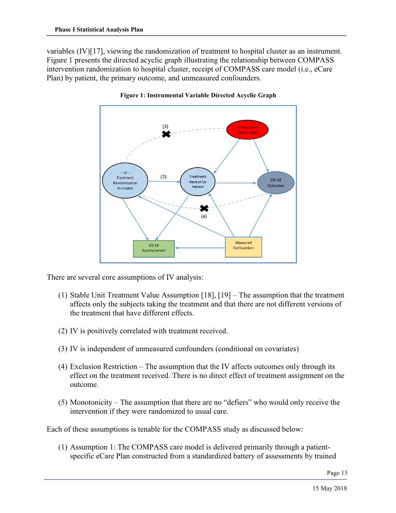
variables (IV)[17], viewing the randomization of treatment to hospital cluster as an instrument.

Figure 1 presents the directed acyclic graph illustrating the relationship between COMPASS

intervention randomization to hospital cluster, receipt of COMPASS care model (i.e., eCare

Plan) by patient, the primary outcome, and unmeasured confounders.

Figure 1: Instrumental Variable Directed Acyclic Graph

There are several core assumptions of IV analysis:

(1) Stable Unit Treatment Value Assumption [18], [19] – The assumption that the treatment

affects only the subjects taking the treatment and that there are not different versions of

the treatment that have different effects.

(2) IV is positively correlated with treatment received.

(3) IV is independent of unmeasured confounders (conditional on covariates)

(4) Exclusion Restriction – The assumption that the IV affects outcomes only through its

effect on the treatment received. There is no direct effect of treatment assignment on the

outcome.

(5) Monotonicity – The assumption that there are no “defiers” who would only receive the

intervention if they were randomized to usual care.

Each of these assumptions is tenable for the COMPASS study as discussed below:

(1) Assumption 1: The COMPASS care model is delivered primarily through a patient-

specific eCare Plan constructed from a standardized battery of assessments by trained


15 May 2018

Page 14

medical personnel who receive comprehensive training during a startup Bootcamp and

consistent reinforcement through ongoing webinars, all of which are led by the

COMPASS Study Implementation Team. There is considerable effort to ensure the model

is implemented consistently across enrolling hospitals. While there is variability in

system-level resources, all hospitals that take part in the COMPASS study have sufficient

infrastructure to administer the care model effectively.

(2) Assumption 2: This assumption holds since one cannot receive the COMPASS care

model at hospitals other than those randomized to the intervention arm in Phase I and

many of the patients who are enrolled at hospitals randomized to administer the

COMPASS intervention do receive the care model as designed.

(3) Assumption 3: The COMPASS study randomization was stratified by whether a hospital

was a primary stroke center and by stroke volume to ensure these important system level

characteristics are independent of treatment assignment.

Our PP analysis will consider adjustment for several patient-level characteristics, which

are believed to be potential confounders to minimize the possibility that any unmeasured

confounder remains correlated with treatment assignment after covariate adjustment.

Candidates for covariate adjustment include: race (white versus non-white), age,

diagnosis (stroke versus TIA), NIHSS, history of stroke or TIA, presence of multiple

comorbidities, ability to ambulate prior to admission, ability to ambulate at discharge,

having a PCP, whether the patient has medical insurance and/or the type of medical

insurance (e.g., private, Medicare, Medicaid, etc.), and number and type of therapy

referrals prior to discharge, and number of and type of therapy referrals prior to

discharge.

(4) Assumption 4: The core component of the COMPASS care model is receipt of an eCare

Plan at the COMPASS clinic visit. Patients are unlikely to benefit meaningfully from the

intervention unless they attend this visit and receive an eCare Plan and so it is unlikely

that patient outcomes are affected by hospital assignment to the COMPASS intervention

by means other than receipt of the customized eCare Plan.

(5) Assumption 5: The assumption of monotonicity (5) is met for the COMPASS Study since

no participants at usual care hospitals are able to receive the COMPASS eCare Plan.

Though there is potential for a participant to enroll at a usual care hospital, experience a

subsequent event and reenroll at an intervention hospital, such an occurrence should be

exceedingly rare.

Two-Stage least squares estimation will be performed for the instrumental variables analysis as

described in [17]. To account for the clustered nature of our data, robust standard errors will be

computed as described in [20]. The first stage regression model will regress the outcome receipt

of an eCare plan at the clinic visit within 30 calendar days onto the hospital-level characteristics

(e.g., stroke volume, primary stroke center status) and a subset of the following patient-level

characteristics: race (white versus non-white), age, diagnosis (stroke versus TIA), NIH Stroke

Scale Score (NIHSS), history of stroke or TIA, presence of multiple comorbidities, ability to


15 May 2018

Page 15

ambulate prior to admission, ability to ambulate at discharge, having a primary care provider

(PCP), whether the patient has medical insurance and/or the type of medical insurance (e.g.,

private, Medicare, Medicaid, etc.), and number and type of therapy referrals prior to discharge.

7.5.1 Correction for Selection Bias Due to Missing Outcomes

Use of instrumental variables offers no protection from selection bias related to outcome

ascertainment [21]. Since the SIS-16 outcome is only ascertained for a subset of patients and

because we have observed a modest imbalance between the two study arms in ascertainment

rates, it is also important to account for any characteristics that influence outcome ascertainment

that are potentially causally related to the outcome of interest. To account for selection bias

associated with outcome ascertainment, we will use the IP weights from the Intent-to-Treat

analysis in the two-stage least squares estimation procedure. This has been shown to improve the

quality of IV estimation in the presence of selection bias [22].

7.5.2 Missing Covariate Data

Due to missing values of some covariates, the two-stage least squares process will be repeated

for 100 datasets with missing data filled in by multiple imputation using MICE. Robust standard

errors will be estimated for each imputed dataset. The results will be combined using standard

techniques [15].

8 ANALYSIS OF SECONDARY ENDPOINTS BASED ON 90-DAY SURVEY DATA

Analysis of the secondary endpoints described in Section 5.2 will be performed using an

analogous strategy to that described for the ITT and PP analyses for the primary outcome.

8.1 Analysis of Modified Caregiver Strain Index Endpoint

The modified CSI is assessed using a caregiver survey that is administered separately from the

90-day participant outcomes survey. The set of factors that influence a caregiver’s propensity to

respond to the caregiver survey may be different from those that influence a participant’s

propensity to response to the 90-day outcomes survey. Accordingly, weighted LMM analyses of

the CSI will weight caregivers based on the inverse of their propensity for CSI outcome

ascertainment estimated using the same procedure as for the primary endpoint. Candidate

predictors for inclusion in the IPW model include the following patient characteristics: race

(white versus non-white), age, diagnosis (stroke versus TIA), NIHSS, history of stroke or TIA,

presence of multiple comorbidities, ability to ambulate prior to admission, ability to ambulate at

discharge, having a PCP, whether the patient has medical insurance, and number and type of

therapy referrals prior to discharge, and number of and type of therapy referrals prior to

discharge. For this endpoint, we will also consider adjustment for gender of the caregiver and

relationship with the participant. Just as with the SIS-16 instrument, the CSI is subject to a

potential ceiling (or floor) effect. Therefore, as necessary, we will perform sensitivity analyses

mirroring those described in Section 7.4.1 for the CSI.

8.2 Analysis of Other Patient-Reported Secondary Endpoints

The mailed survey that is sent after sufficient unsuccessful attempts to complete the 90-day

outcomes call only collects the SIS-16, self-rated health, and blood pressure endpoint data. For

analysis of these secondary endpoints, the propensity scores from the primary endpoint analysis


15 May 2018

Page 16

will be used. For secondary endpoints only collected by phone, separate propensity scores will be

estimated. Depending on the nature of the secondary endpoint, the analysis model will be a linear

mixed model (continuous endpoints), a logistic mixed model (binary endpoints), or an ordinal

logistic mixed model (multi-category ordinal endpoints). The set of potential confounders that

are relevant to the analysis of each of the secondary endpoints will vary (e.g., history of

hypertension will be highly relevant to BP related outcomes but not so for many other secondary

endpoints).

Several secondary endpoints are defined based on a standardized instrument that has a small

number of items (e.g., MoCA, PROMIS Fatigue Instrument, MGLS-4, and PHQ-2). In these

cases, partial completion of the instrument results in a sizeable fraction of missing information

on the outcome. In instances where one or more items on such instruments are missing,

remaining missing items will be imputed using MICE for analysis. The imputation model will be

based on the non-missing items for the instrument and baseline characteristics relevant to the

endpoint in question. Because partially completed instruments will have missing values imputed,

propensity score models will include partial completion as an observed outcome.

9 SUBGROUP ANALYSES

For reasons described in Section 7.3, the primary analysis will assess the degree to which the

effect of the COMPASS Intervention varies with patient diagnosis (stroke versus TIA). In

addition to this assessment, it is of a priori interest to examine the comparative effectiveness of

the COMPASS Intervention in key subgroups of the studied population. We will examine the

comparative effectiveness of the COMPASS Intervention in the following subgroups:

Race – White, Non-White

Sex – Male, Female

Age – <45, 45-<55, 55-<65, 65-<75, >=75

Stroke severity – NIHSS=0, NIHSS=1-4, NIHSS>4

Type of Health Insurance – Insured versus uninsured

For each of the characteristic above (e.g., race) and to the extent that samples size permits, we

will evaluate the comparative effectiveness of the COMPASS Intervention against usual care

within each of the corresponding subgroups (e.g., for whites and non-whites) using methodology

analogous to that previously described for the primary and secondary endpoints. For a given

endpoint and characteristic, a single model will be fit for all subgroups and will include

subgroup-specific treatment effects.


15 May 2018

Page 17

BIBLIOGRAPHY

[1] P. W. Duncan et al., “The Comprehensive Post-Acute Stroke Services (COMPASS)

study: design and methods for a cluster-randomized pragmatic trial,” BMC Neurol., vol.

17, no. 1, p. 133, Jul. 2017.

[2] P. W. Duncan, S. M. Lai, R. K. Bode, S. Perera, and J. DeRosa, “Stroke impact scale-16:

A brief assessment of physical function,” Neurology, vol. 60, no. 2, pp. 291–296, Jan.

2003.

[3] M. Thornton and S. S. Travis, “Analysis of the reliability of the modified caregiver strain

index.,” J. Gerontol. B. Psychol. Sci. Soc. Sci., vol. 58, no. 2, pp. S127–S132, Mar. 2003.

[4] P. Diehr, J. Williamson, D. L. Patrick, D. E. Bild, and G. L. Burke, “Patterns of self-rated

health in older adults before and after sentinel health events,” J. Am. Geriatr. Soc., vol. 49,

no. 1, pp. 36–44, Jan. 2001.

[5] A. Wong et al., “Montreal Cognitive Assessment 5-Minute Protocol Is a Brief, Valid,

Reliable, and Feasible Cognitive Screen for Telephone Administration,” Stroke, 2015.

[6] Z. S. Nasreddine et al., “The Montreal Cognitive Assessment, MoCA: A Brief Screening

Tool For Mild Cognitive Impairment,” J. Am. Geriatr. Soc., vol. 53, no. 4, pp. 695–699,

Apr. 2005.

[7] K. Kroenke, R. L. Spitzer, and J. B. W. Williams, “The Patient Health Questionnaire-2:

validity of a two-item depression screener.,” Med. Care, vol. 41, no. 11, pp. 1284–92,

Nov. 2003.

[8] J.-S. Lai et al., “How item banks and their application can influence measurement practice

in rehabilitation medicine: a PROMIS fatigue item bank example.,” Arch. Phys. Med.

Rehabil., vol. 92, no. 10 Suppl, pp. S20-7, Oct. 2011.

[9] J. C. van Swieten, P. J. Koudstaal, M. C. Visser, H. J. Schouten, and J. van Gijn,

“Interobserver agreement for the assessment of handicap in stroke patients.,” Stroke, vol.

19, no. 5, pp. 604–7, May 1988.

[10] D. E. Morisky, L. W. Green, and D. M. Levine, “Concurrent and Predictive Validity of a

Self-Reported Measure of Medication Adherence,” Medical Care, vol. 24. Lippincott

Williams & Wilkins, pp. 67–74.

[11] C. E. Frangakis and D. B. Rubin, “Principal Stratification in Causal Inference,”

Biometrics, vol. 58, no. 1, pp. 21–29, Mar. 2002.

[12] M. G. Kenward and J. H. Roger, “Small Sample Inference for Fixed Effects from

Restricted Maximum Likelihood,” Biometrics, vol. 53, no. 3, p. 983, Sep. 1997.

[13] C. J. Skinner and D’arrigo, “Inverse probability weighting for clustered nonresponse,”

Biometrika, vol. 98, no. 4, pp. 953–966, Dec. 2011.

[14] S. van Buuren, “Multiple imputation of discrete and continuous data by fully conditional

specification,” Stat. Methods Med. Res., vol. 16, no. 3, pp. 219–242, Jun. 2007.

[15] D. B. Rubin, Multiple imputation for nonresponse in surveys. Wiley-Interscience, 2004.

[16] G. HOMMEL, “A comparison of two modified Bonferroni procedures,” Biometrika, vol.

76, no. 3, pp. 624–625, Sep. 1989.

[17] M. Baiocchi, J. Cheng, and D. S. Small, “Instrumental variable methods for causal

inference.,” Stat. Med., vol. 33, no. 13, pp. 2297–340, Jun. 2014.

[18] J. D. Angrist, G. W. Imbens, and D. B. Rubin, “Identification of Causal Effects Using

Instrumental Variables,” J. Am. Stat. Assoc., vol. 91, no. 434, pp. 444–455, 1996.

[19] J. D. Angrist, G. W. Imbens, and D. B. Rubin, “Identification of Causal Effects Using


15 May 2018

Page 18

Instrumental Variables: Rejoinder,” J. Am. Stat. Assoc., vol. 91, no. 434, p. 468, Jun.

1996.

[20] H. White, “Instrumental Variables Regression with Independent Observations,”

Econometrica, vol. 50, no. 2, p. 483, Mar. 1982.

[21] R. A. Hughes, N. M. Davies, G. Davey Smith, and K. Tilling, “Selection bias in

instrumental variable analyses,” bioRxiv, Jan. 2017.

[22] C. Canan, C. Lesko, and B. Lau, “Instrumental Variable Analyses and Selection Bias,”

Epidemiology, vol. 28, no. 3, pp. 396–398, May 2017.

Phase 1 Statistical Analysis Plan - clinicaltrials.gov · on race, sex, age, diagnosis (stroke...

Documents

Transcript of Phase 1 Statistical Analysis Plan - clinicaltrials.gov · on race, sex, age, diagnosis (stroke...