
PHAS3201: Electromagnetic Theory
109
PHAS3201: Electromagnetic Theory Stan Zochowski December 17, 2011
Transcript of PHAS3201: Electromagnetic Theory
PHAS3201: Electromagnetic Theory
Stan Zochowski
December 17, 2011
PHAS3201: Electromagnetic Theory
2011 2
PHAS3201: Electromagnetic Theory CONTENTS
Contents
1 Introduction 71.1 Mathematical Tools . . . . . . . . . . . . . . . . . . . . . . . . . . . . . . . . . . . . . . . . . . . . . . 71.2 Overview of PHAS2201 . . . . . . . . . . . . . . . . . . . . . . . . . . . . . . . . . . . . . . . . . . . 8
1.2.1 Fields . . . . . . . . . . . . . . . . . . . . . . . . . . . . . . . . . . . . . . . . . . . . . . . . . 81.2.2 Electrostatics . . . . . . . . . . . . . . . . . . . . . . . . . . . . . . . . . . . . . . . . . . . . . 91.2.3 Magnetostatics . . . . . . . . . . . . . . . . . . . . . . . . . . . . . . . . . . . . . . . . . . . . 101.2.4 Electromagnetism . . . . . . . . . . . . . . . . . . . . . . . . . . . . . . . . . . . . . . . . . . 10
2 Macroscopic Fields 132.1 Reminder of PHAS2201 . . . . . . . . . . . . . . . . . . . . . . . . . . . . . . . . . . . . . . . . . . . 13
2.1.1 Electrostatics . . . . . . . . . . . . . . . . . . . . . . . . . . . . . . . . . . . . . . . . . . . . . 132.1.2 Dielectrics . . . . . . . . . . . . . . . . . . . . . . . . . . . . . . . . . . . . . . . . . . . . . . 14
2.2 Electric Field in Dielectric Media . . . . . . . . . . . . . . . . . . . . . . . . . . . . . . . . . . . . . . . 152.3 Magnetic Fields Revision . . . . . . . . . . . . . . . . . . . . . . . . . . . . . . . . . . . . . . . . . . . 202.4 Magnetic Vector Potential . . . . . . . . . . . . . . . . . . . . . . . . . . . . . . . . . . . . . . . . . . . 222.5 Magnetic Intensity . . . . . . . . . . . . . . . . . . . . . . . . . . . . . . . . . . . . . . . . . . . . . . 232.6 Interfaces and Boundary Conditions . . . . . . . . . . . . . . . . . . . . . . . . . . . . . . . . . . . . . 252.7 Summary of Linear Media . . . . . . . . . . . . . . . . . . . . . . . . . . . . . . . . . . . . . . . . . . 27
3 Atomic Mechanisms 293.1 Dipoles and Polarization . . . . . . . . . . . . . . . . . . . . . . . . . . . . . . . . . . . . . . . . . . . 293.2 Magnetic Dipole . . . . . . . . . . . . . . . . . . . . . . . . . . . . . . . . . . . . . . . . . . . . . . . 363.3 Magnetic Dipoles and Magnetization . . . . . . . . . . . . . . . . . . . . . . . . . . . . . . . . . . . . . 403.4 Diamagnetism and Paramagnetism . . . . . . . . . . . . . . . . . . . . . . . . . . . . . . . . . . . . . . 45
4 Ferromagnetism 474.1 Atomic-level Picture . . . . . . . . . . . . . . . . . . . . . . . . . . . . . . . . . . . . . . . . . . . . . 474.2 B & H: Macroscopic Effects . . . . . . . . . . . . . . . . . . . . . . . . . . . . . . . . . . . . . . . . . 504.3 Simple Examples of Electromagnetic Systems . . . . . . . . . . . . . . . . . . . . . . . . . . . . . . . . 53
4.3.1 Solenoid . . . . . . . . . . . . . . . . . . . . . . . . . . . . . . . . . . . . . . . . . . . . . . . 534.3.2 Bar Magnet . . . . . . . . . . . . . . . . . . . . . . . . . . . . . . . . . . . . . . . . . . . . . . 564.3.3 Toroid . . . . . . . . . . . . . . . . . . . . . . . . . . . . . . . . . . . . . . . . . . . . . . . . . 574.3.4 Fluxmeter . . . . . . . . . . . . . . . . . . . . . . . . . . . . . . . . . . . . . . . . . . . . . . . 58
4.4 Energy Density . . . . . . . . . . . . . . . . . . . . . . . . . . . . . . . . . . . . . . . . . . . . . . . . 594.5 Summaries . . . . . . . . . . . . . . . . . . . . . . . . . . . . . . . . . . . . . . . . . . . . . . . . . . 60
5 Maxwell’s Equations and EM Waves 635.1 Displacement Current . . . . . . . . . . . . . . . . . . . . . . . . . . . . . . . . . . . . . . . . . . . . . 635.2 Maxwell’s Equations . . . . . . . . . . . . . . . . . . . . . . . . . . . . . . . . . . . . . . . . . . . . . 65
5.2.1 Differential Form . . . . . . . . . . . . . . . . . . . . . . . . . . . . . . . . . . . . . . . . . . . 655.2.2 Integral Form . . . . . . . . . . . . . . . . . . . . . . . . . . . . . . . . . . . . . . . . . . . . . 655.2.3 Wave Equations . . . . . . . . . . . . . . . . . . . . . . . . . . . . . . . . . . . . . . . . . . . . 66
5.3 Plane Waves . . . . . . . . . . . . . . . . . . . . . . . . . . . . . . . . . . . . . . . . . . . . . . . . . . 675.4 Polarization . . . . . . . . . . . . . . . . . . . . . . . . . . . . . . . . . . . . . . . . . . . . . . . . . . 68
2011 3
PHAS3201: Electromagnetic Theory CONTENTS
6 Reflection & Refraction 716.1 Refractive Index . . . . . . . . . . . . . . . . . . . . . . . . . . . . . . . . . . . . . . . . . . . . . . . . 71
6.1.1 Origin . . . . . . . . . . . . . . . . . . . . . . . . . . . . . . . . . . . . . . . . . . . . . . . . . 716.1.2 Phase velocity . . . . . . . . . . . . . . . . . . . . . . . . . . . . . . . . . . . . . . . . . . . . 72
6.2 Reflection & Refraction . . . . . . . . . . . . . . . . . . . . . . . . . . . . . . . . . . . . . . . . . . . . 726.2.1 Geometry . . . . . . . . . . . . . . . . . . . . . . . . . . . . . . . . . . . . . . . . . . . . . . . 726.2.2 Two Laws: Reflection & Refraction . . . . . . . . . . . . . . . . . . . . . . . . . . . . . . . . . 736.2.3 Changes of Amplitude . . . . . . . . . . . . . . . . . . . . . . . . . . . . . . . . . . . . . . . . 746.2.4 Fresnel Relations . . . . . . . . . . . . . . . . . . . . . . . . . . . . . . . . . . . . . . . . . . . 76
6.3 Special Angles . . . . . . . . . . . . . . . . . . . . . . . . . . . . . . . . . . . . . . . . . . . . . . . . 766.3.1 Brewster Angle . . . . . . . . . . . . . . . . . . . . . . . . . . . . . . . . . . . . . . . . . . . . 766.3.2 Critical Angle . . . . . . . . . . . . . . . . . . . . . . . . . . . . . . . . . . . . . . . . . . . . . 776.3.3 Total Internal Reflection . . . . . . . . . . . . . . . . . . . . . . . . . . . . . . . . . . . . . . . 786.3.4 Intensities . . . . . . . . . . . . . . . . . . . . . . . . . . . . . . . . . . . . . . . . . . . . . . . 79
7 Waves in Conducting Media 817.1 Conductors . . . . . . . . . . . . . . . . . . . . . . . . . . . . . . . . . . . . . . . . . . . . . . . . . . 81
7.1.1 Origins . . . . . . . . . . . . . . . . . . . . . . . . . . . . . . . . . . . . . . . . . . . . . . . . 817.1.2 Dispersion Relation . . . . . . . . . . . . . . . . . . . . . . . . . . . . . . . . . . . . . . . . . . 817.1.3 Good Conductors . . . . . . . . . . . . . . . . . . . . . . . . . . . . . . . . . . . . . . . . . . . 817.1.4 Skin depth . . . . . . . . . . . . . . . . . . . . . . . . . . . . . . . . . . . . . . . . . . . . . . 82
7.2 Reflection At Metal Surface . . . . . . . . . . . . . . . . . . . . . . . . . . . . . . . . . . . . . . . . . 837.2.1 Refractive Index . . . . . . . . . . . . . . . . . . . . . . . . . . . . . . . . . . . . . . . . . . . 83
7.3 Plasmas . . . . . . . . . . . . . . . . . . . . . . . . . . . . . . . . . . . . . . . . . . . . . . . . . . . . 847.3.1 Plasma Frequency . . . . . . . . . . . . . . . . . . . . . . . . . . . . . . . . . . . . . . . . . . 847.3.2 Dispersion . . . . . . . . . . . . . . . . . . . . . . . . . . . . . . . . . . . . . . . . . . . . . . 85
8 Energy Flow and the Poynting Vector 898.1 Poynting’s Theorem . . . . . . . . . . . . . . . . . . . . . . . . . . . . . . . . . . . . . . . . . . . . . . 89
8.1.1 Energy Densities . . . . . . . . . . . . . . . . . . . . . . . . . . . . . . . . . . . . . . . . . . . 898.1.2 Energy Flow . . . . . . . . . . . . . . . . . . . . . . . . . . . . . . . . . . . . . . . . . . . . . 908.1.3 Poynting’s Theorem . . . . . . . . . . . . . . . . . . . . . . . . . . . . . . . . . . . . . . . . . 908.1.4 Average flow . . . . . . . . . . . . . . . . . . . . . . . . . . . . . . . . . . . . . . . . . . . . . 91
8.2 Pressure due to EM Waves . . . . . . . . . . . . . . . . . . . . . . . . . . . . . . . . . . . . . . . . . . 918.2.1 Photons . . . . . . . . . . . . . . . . . . . . . . . . . . . . . . . . . . . . . . . . . . . . . . . . 91
9 Emission of Radiation 939.1 Retarded Potentials . . . . . . . . . . . . . . . . . . . . . . . . . . . . . . . . . . . . . . . . . . . . . . 93
9.1.1 Fields . . . . . . . . . . . . . . . . . . . . . . . . . . . . . . . . . . . . . . . . . . . . . . . . . 939.1.2 Lorentz Condition . . . . . . . . . . . . . . . . . . . . . . . . . . . . . . . . . . . . . . . . . . 949.1.3 Wave Equations . . . . . . . . . . . . . . . . . . . . . . . . . . . . . . . . . . . . . . . . . . . . 949.1.4 Retarded Time . . . . . . . . . . . . . . . . . . . . . . . . . . . . . . . . . . . . . . . . . . . . 95
9.2 Hertzian Dipole . . . . . . . . . . . . . . . . . . . . . . . . . . . . . . . . . . . . . . . . . . . . . . . . 969.2.1 Geometry . . . . . . . . . . . . . . . . . . . . . . . . . . . . . . . . . . . . . . . . . . . . . . . 969.2.2 Potentials . . . . . . . . . . . . . . . . . . . . . . . . . . . . . . . . . . . . . . . . . . . . . . . 98
10 Relativistic Transformations 10110.1 Introduction . . . . . . . . . . . . . . . . . . . . . . . . . . . . . . . . . . . . . . . . . . . . . . . . . . 101
10.1.1 Basic Principles . . . . . . . . . . . . . . . . . . . . . . . . . . . . . . . . . . . . . . . . . . . . 10110.1.2 Coordinate transforms . . . . . . . . . . . . . . . . . . . . . . . . . . . . . . . . . . . . . . . . 10110.1.3 Interval . . . . . . . . . . . . . . . . . . . . . . . . . . . . . . . . . . . . . . . . . . . . . . . . 10210.1.4 Lorentz transformation . . . . . . . . . . . . . . . . . . . . . . . . . . . . . . . . . . . . . . . . 103
10.2 Four-vectors . . . . . . . . . . . . . . . . . . . . . . . . . . . . . . . . . . . . . . . . . . . . . . . . . . 10410.2.1 Position-Time 4-vector . . . . . . . . . . . . . . . . . . . . . . . . . . . . . . . . . . . . . . . . 10410.2.2 Other 4-vectors . . . . . . . . . . . . . . . . . . . . . . . . . . . . . . . . . . . . . . . . . . . . 105
10.3 Transformations of Fields . . . . . . . . . . . . . . . . . . . . . . . . . . . . . . . . . . . . . . . . . . . 10510.3.1 Current Density . . . . . . . . . . . . . . . . . . . . . . . . . . . . . . . . . . . . . . . . . . . . 105
2011 4
PHAS3201: Electromagnetic Theory CONTENTS
10.3.2 Potentials . . . . . . . . . . . . . . . . . . . . . . . . . . . . . . . . . . . . . . . . . . . . . . . 10610.3.3 Fields . . . . . . . . . . . . . . . . . . . . . . . . . . . . . . . . . . . . . . . . . . . . . . . . . 10610.3.4 Maxwell’s Equations . . . . . . . . . . . . . . . . . . . . . . . . . . . . . . . . . . . . . . . . . 10710.3.5 Transformations . . . . . . . . . . . . . . . . . . . . . . . . . . . . . . . . . . . . . . . . . . . 108
2011 5
PHAS3201: Electromagnetic Theory CONTENTS
2011 6
PHAS3201: Electromagnetic Theory CHAPTER 1. INTRODUCTION
Chapter 1
Introduction
Office hours: anytime you can find me, or email me ([email protected]) to set a time. Attendance sheets must befilled in. They’ll be given out at the start of a lecture and collated over the weeks.
Problem sheets will be given out through the term, roughly every two weeks. As detailed in the Preliminaries, the bestthree problem sheets will count for 10% of the final course mark. N.B. There will be four sheets during term.
Full sets of lecture notes will be made available a few days after the lecture. A complete PDF file will be available atthe end of the course.
1.1 Mathematical ToolsThe easy use of mathematical tools is vital to understanding electromagnetic theory.
• The differential operators transform vectors and scalars:
Grad : scalar to vector F(r) = ∇ϕ(r) (1.1)
=
(∂ϕ
∂xi +
∂ϕ
∂yj +
∂ϕ
∂zk
)(1.2)
Div : vector to scalar q(r) =∇ · F(r) (1.3)
=∂Fx∂x
+∂Fy∂y
+∂Fz∂z
(1.4)
Curl : vector to vector G(r) = ∇× F(r) (1.5)
=
∣∣∣∣∣∣i j k∂∂x
∂∂y
∂∂z
Fx Fy Fz
∣∣∣∣∣∣ (1.6)
• These are also given in the Preliminaries handout for other coordinate systems;
• They should be reasonably familiar.
These should be reasonably familiar from the courses in the first and second years. Hopefully we won’t have to spendmuch time on them, but they are important.
• Integrals of vectors can produce scalars or vectors;
• There are 1-, 2- and 3-D integrals (line, surface and volume);
• These are all important in Electromagnetic theory!
• There are important theorems relating integrals of the differential operators:
• Divergence Theorem: ∫V
∇ · Fdv =
∮S
F · nda (1.7)
2011 7
PHAS3201: Electromagnetic Theory CHAPTER 1. INTRODUCTION
• Stokes’ Theorem: ∫S
∇× F · nda =
∮C
F · dl (1.8)
• Notice the importance of∮
!
It’s useful to understand how a line integral works by considering the basic definition in terms of small steps:∫ b
a C
F · dl = limN→∞
N∑i=1
Fi · dli, (1.9)
where C is the curve we’re integrating along. In other words, at each point along the curve we take the dot productbetween the function we’re integrating and the tangent to the curve, and then sum over all these points. It should be easyto see that, in general, the value of the line integral will depend on the curve chosen.
There are two standard ways of working out a line integral. If you are given F (x, y) along some line g(x, y), thenwe can replace every occurrence of y and dy in the integral below with some functions of x (found from g(x, y)) andintegrate: ∫
C
F · dl =
∫C
Fx(x, y)dx+ Fy(x, y)dy (1.10)
=
∫C
Fx(x, y(x))dx+ Fy(x, y(x))dy
dxdx. (1.11)
The second way is using a parametric form. This is possible if the curve being used for the integral is given in termsof a parameter (e.g. angle around a circle). Then we have a curve l(t) which depends on a single parameter t. So wewrite: ∫
C
F · dl =
∫ b
a
F(l(t)) · dldtdt (1.12)
=
∫ b
a
Fx (x(t), y(t))dx
dtdt+ Fy (x(t), y(t))
dy
dtdt (1.13)
One important result is: ∫ b
a
∇ϕ · dl = ϕ(b)− ϕ(a), (1.14)
so that the line integral of a gradient is independent of path.Surface integrals can be evaluated in a similar way, and we expect to have a surface defined; one way is like this:
r(u, v) = x(u, v)i + y(u, v)j + z(u, v)k. (1.15)
Then we know that ∂r∂u ×∂r∂v is orthogonal to the surface. It is also useful to remember that for a plane passing through a
point r0, the normal is defined as:
n · (r− r0) = 0 (1.16)⇒ (a, b, c) · (x− x0, y − y0, z − z0) = 0. (1.17)
It’s clear that a plane whose equation is ax+ by + cz = d has a normal vector given by (a, b, c).
1.2 Overview of PHAS2201
1.2.1 Fields• In a vacuum, the basic fields are E and B;
• What are they? What are their units?
• When they interact with matter, there are changes;
2011 8
PHAS3201: Electromagnetic Theory CHAPTER 1. INTRODUCTION
• Why should this happen?
• We have the the fields D and H, with D = ε0E + P and B = µ0(H + M) where M is the magnetization;
• Be careful that you know what you’re dealing with!
The electric and magnetic fields have SI units of newtons per coulomb (or volts per metre) and tesla (equivalent tokilograms per coulomb second!). Be careful with units: Gaussian units are quite different. Note that B is often called themagnetic induction field, or simply the magnetic induction.
Matter responds to fields: the atoms of molecules polarize in an electric field, and respond in varied ways to a magneticfield (both diminishing and amplifying it). The fields D and H reflect this.
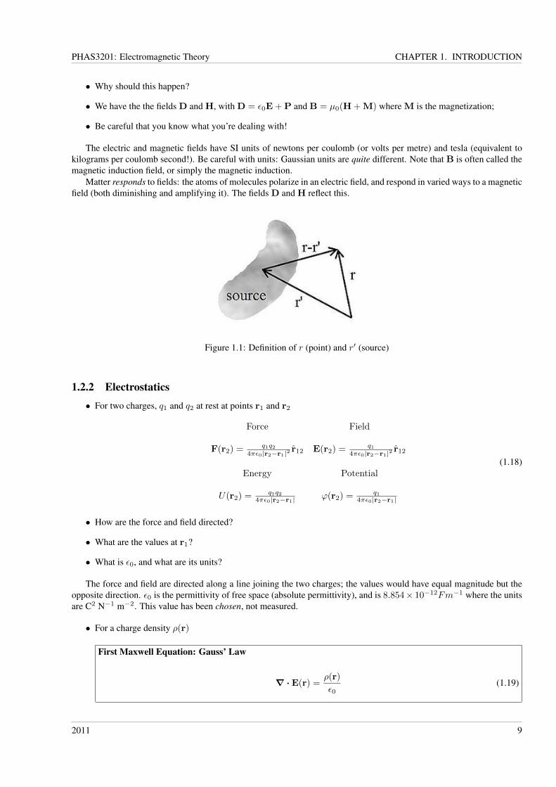
Figure 1.1: Definition of r (point) and r′ (source)
1.2.2 Electrostatics• For two charges, q1 and q2 at rest at points r1 and r2
Force Field
F(r2) = q1q24πε0|r2−r1|2
r12 E(r2) = q14πε0|r2−r1|2
r12
Energy Potential
U(r2) = q1q24πε0|r2−r1| ϕ(r2) = q1
4πε0|r2−r1|
(1.18)
• How are the force and field directed?
• What are the values at r1?
• What is ε0, and what are its units?
The force and field are directed along a line joining the two charges; the values would have equal magnitude but theopposite direction. ε0 is the permittivity of free space (absolute permittivity), and is 8.854× 10⁻¹²Fm−1 where the unitsare C2 N−1 m−2. This value has been chosen, not measured.
• For a charge density ρ(r)
First Maxwell Equation: Gauss’ Law
∇ ·E(r) =ρ(r)
ε0(1.19)
2011 9

PHAS3201: Electromagnetic Theory CHAPTER 1. INTRODUCTION
• This can also be written for a collection of charges:∮E · nda =
1
ε0
∑i
qi (1.20)
• The integral and differential forms are linked by the divergence theorem
Note that∑i qi =
∫Vρdv
1.2.3 Magnetostatics• For an element of a current loop, dl, carrying current I at r′:
dB(r) =µ0I
4π
dl× (r− r′)
|r− r′|3(1.21)
• We can perform a loop integral:
B =µ0I
4π
∮C
dl× (r− r′)
|r− r′|3(1.22)
• Because∇ ·∇× F = 0, we can show that there is a magnetic vector potential A such that B =∇×A, so
Second Maxwell Equation: No Magnetic Monopoles
∇ ·B = 0 (1.23)
• What is µ0, and what are its units?
Remember that the Biot-Savart law is empirical: there is no underlying theory stating that there are no magnetic monopolesin the universe. But we haven’t found any yet! The result derived from the Biot-Savart law is the second Maxwell equa-tion.
µ0 is the permeability of free space, and is 4π×10−7T m A−1 (which is equivalent to kilograms metres per coulomb2).
1.2.4 Electromagnetism• For a surface S bounded by loop C, ∮
c
B · dl = µ0I, (1.24)
• where I is the current passing through the surface S
• We can write I as∫SJ · nda
• Using Stokes’ Theorem, we find:∮c
B · dl =
∫S
∇×B · nda = µ0I =
∫S
µ0J · nda (1.25)
Third Maxwell Equation: Ampère’s law
∇×B = µ0J (1.26)
• This is incomplete.
2011 10
PHAS3201: Electromagnetic Theory CHAPTER 1. INTRODUCTION
We will consider the detailed form of why Ampère’s law is incomplete later in the lectures, though you should alreadyhave seen this and understood it at some level. This will form our third Maxwell equation when complete.
• If a conducting circuit, C, is intersected by a B field, then the flux is given by:
ΦC =
∫S
B · nda (1.27)
• The EMF induced around the circuit isE = −dΦ
dt=
∮C
E · dl (1.28)
• As before, we can use Stokes’ Theorem to write:∫S
dB
dt· nda = −
∮C
E · dl = −∫S
∇×E · nda (1.29)
and derive:
Fourth Maxwell Equation: Faraday’s Law
∇×E = −dBdt
(1.30)
As you can see, the derivation is almost trivial: substitute Eq. (1.27) into Eq. (1.28), and then apply Stokes’ theoremto the loop integral of E. This is the final Maxwell equation.
• Ampère’s law as described above is incomplete: it needs to account for time-varying electric fields
• When we do this, we can write (in a vacuum):
Maxwell’s Equations:
∇ ·E =ρ
ε0(1.31)
∇ ·B = 0 (1.32)
∇×B = µ0J + µ0ε0dE
dt(1.33)
∇×E = −dBdt
(1.34)
• To complete our set of equations, we have the force on a moving charge:
Lorentz Force
F = q (E + v ×B) (1.35)
Once Maxwell’s equations and the Lorentz force law have been specified, classical electromagnetism is essentiallycomplete: the basic physics has not changed, though the details of the interaction of the fields with matter are still beingunderstood.
2011 11
PHAS3201: Electromagnetic Theory CHAPTER 1. INTRODUCTION
2011 12
PHAS3201: Electromagnetic Theory CHAPTER 2. MACROSCOPIC FIELDS
Chapter 2
Macroscopic Fields
Maxwell’s equations have two major variants: the microscopic set of Maxwell’s equations uses total charge and total cur-rent including the difficult-to-calculate atomic level charges and currents in materials. The macroscopic set of Maxwell’sequations defines two new auxiliary fields that can sidestep having to know these ’atomic’ sized charges and currents.Unlike the ’microscopic’ equations, "Maxwell’s macroscopic equations", also known as Maxwell’s equations in matter,factor out the bound charge and current to obtain equations that depend only on the free charges and currents. Theseequations are more similar to those that Maxwell himself introduced. The cost of this factorization is that additional fieldsneed to be defined: the displacement field D which is defined in terms of the electric field E and the polarization P ofthe material, and the magnetic-H field, which is defined in terms of the magnetic-B field and the magnetization M of thematerial. In this chapter, we will look at these macroscopic fields, D and H.
2.1 Reminder of PHAS2201We begin this section of the course by going over electrostatic concepts which should be very familiar from PHAS2201,including Gauss’ law and the effect of dielectrics on capacitance.
2.1.1 Electrostatics• We start with a single charge, q, at r′:
E(r) = q(r− r′)/(4πε0|r− r′|3) (2.1)
• Taking a surface integral gives∮SE.nda = q/ε0
• Increasing the number of charges, and using the principle of superposition, we get:∮S
E.nda =
∫ρdv/ε0 (2.2)
• This leads directly to Gauss’ law: ∇ ·E = ρ/ε0
We will now go through a few worked examples on the use of Gauss’ Law.
Ex. 1 — Find the electric field inside a sphere which carries a charge density proportional to the distance from the origin,ρ = kr, for some constant k.
Ex. 2 — A long coaxial cable carries a uniform volume charge density ρ on the inner cylinder (radius a), and a uniformsurface charge density on the outer cylindrical shell (radius b). This surface charge is negative and of just the rightmagnitude so that the cable as a whole is electrically neutral. Find the electric field in each of the three regions: (i) insidethe inner cylinder (r < a), (ii) between the cylinders (a < r < b), (iii) outside the cable (r > b). Plot |E| as a function ofr.
2011 13
PHAS3201: Electromagnetic Theory CHAPTER 2. MACROSCOPIC FIELDS
2.1.2 DielectricsA dielectric is an electrical insulator that can be polarized by an applied electric field. When a dielectric is placed in anelectric field, electric charges do not flow through the material, as in a conductor, but only slightly shift from their averageequilibrium positions causing dielectric polarization. Because of dielectric polarization, positive charges are displacedtoward the field and negative charges shift in the opposite direction. This creates an internal electric field which reducesthe overall field within the dielectric itself.
• Recall that capacitance is defined by Q = C∆V
• Capacitance changes when a dielectric is added:
Cdielectric = κCvacuum (2.3)
• A dielectric has no free charges: an insulator
• The polarization is P = ε0χeE (and is defined as dipole moment per unit volume)
• This gives the susceptibility, χe
• The dielectric constant is κ = 1 + χe
Polarization reflects the fact that the atoms which make up the dielectric consist of separate positive (nucleus) andnegative (electrons) charges. These respond differently to the electric field, leading to a shift in the overall charge distri-bution of the dielectric, while keeping it neutral. We will consider the microscopic origin of polarization in detail in nextsection of the course.
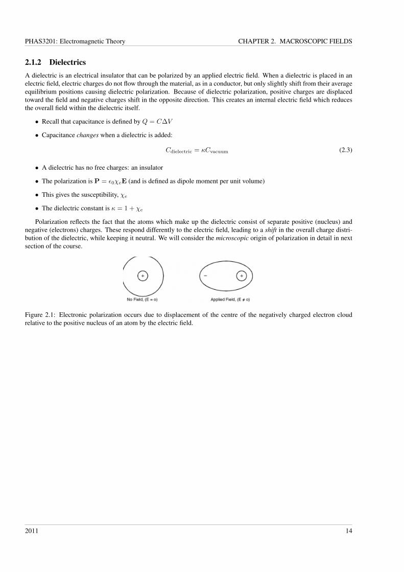
Figure 2.1: Electronic polarization occurs due to displacement of the centre of the negatively charged electron cloudrelative to the positive nucleus of an atom by the electric field.
2011 14
PHAS3201: Electromagnetic Theory CHAPTER 2. MACROSCOPIC FIELDS
2.2 Electric Field in Dielectric Media• We want to develop a theory for electric fields in the presence of polarized media
• We will start by consider the field outside a piece of polarized dielectric
• This will introduce the ideas of polarization charge densities
• Then we will move onto the field inside a piece of polarized dielectric
• We will find a useful reformulation of Gauss’ Law
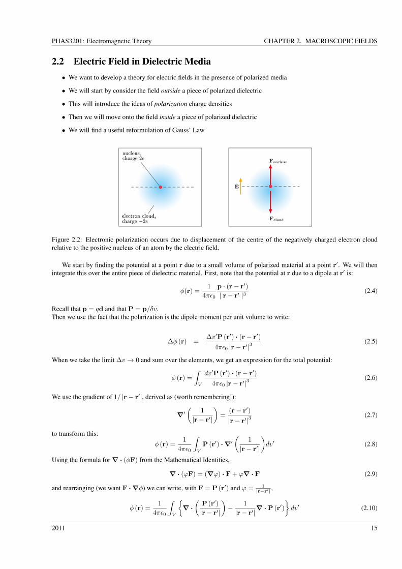
Figure 2.2: Electronic polarization occurs due to displacement of the centre of the negatively charged electron cloudrelative to the positive nucleus of an atom by the electric field.
We start by finding the potential at a point r due to a small volume of polarized material at a point r′. We will thenintegrate this over the entire piece of dielectric material. First, note that the potential at r due to a dipole at r′ is:
φ(r) =1
4πε0
p · (r− r′)
| r− r′ |3(2.4)
Recall that p = qd and that P = p/δv.Then we use the fact that the polarization is the dipole moment per unit volume to write:
∆φ (r) =∆v′P (r′) · (r− r′)
4πε0 |r− r′|3(2.5)
When we take the limit ∆v → 0 and sum over the elements, we get an expression for the total potential:
φ (r) =
∫V
dv′P (r′) · (r− r′)
4πε0 |r− r′|3(2.6)
We use the gradient of 1/ |r− r′|, derived as (worth remembering!):
∇′(
1
|r− r′|
)=
(r− r′)
|r− r′|3(2.7)
to transform this:
φ (r) =1
4πε0
∫V
P (r′) · ∇′(
1
|r− r′|
)dv′ (2.8)
Using the formula for∇ · (φF) from the Mathematical Identities,
∇ · (ϕF) = (∇ϕ) · F + ϕ∇ · F (2.9)
and rearranging (we want F · ∇φ) we can write, with F = P (r′) and ϕ = 1|r−r′| ,
φ (r) =1
4πε0
∫V
{∇ ·
(P (r′)
|r− r′|
)− 1
|r− r′|∇ ·P (r′)
}dv′ (2.10)
2011 15
PHAS3201: Electromagnetic Theory CHAPTER 2. MACROSCOPIC FIELDS
Finally, we use the divergence theorem on the first term[∫V∇ · Fdv =
∮SF · nda
], to give the potential outside a
polarized dielectric object:
φ (r) =1
4πε0
∮S
P (r′) · n|r− r′|
da′ +1
4πε0
∫V
−∇ ·P (r′)
|r− r′|dv′ (2.11)
• The surface polarization charge density is defined:
σP = P · n (2.12)
• The volume polarization charge density is defined:
ρP = −∇ ·P (2.13)
• We can write the potential as:
φ (r) =1
4πε0
(∮S
σP|r− r′|
da′ +
∫V
ρP|r− r′|
dv′)
(2.14)
=1
4πε0
∫dqP|r− r′|
(2.15)
For uniform polarization,∇ · P = 0, so there is no bound charge within the material, but there will be bound chargeon the surface.
Bound charge: The charge within a material that is unable to move freely through the material. Small displacementsof bound charge are responsible for polarization of a material by an electric field.
Free charge: The charge in a conducting material associated with the conduction electrons that are free to movethroughout the material. These electrons can carry electric current.
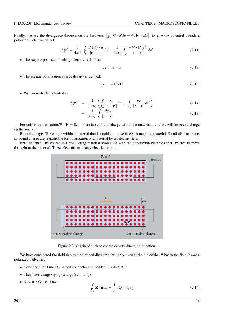
Figure 2.3: Origin of surface charge density due to polarization.
We have considered the field due to a polarized dielectric, but only outside the dielectric. What is the field inside apolarized dielectric?
• Consider three (small) charged conductors embedded in a dielectric
• They have charges q1, q2 and q3 (sum to Q)
• Now use Gauss’ Law: ∮S
E · nda =1
ε0(Q+QP ) (2.16)
2011 16
PHAS3201: Electromagnetic Theory CHAPTER 2. MACROSCOPIC FIELDS
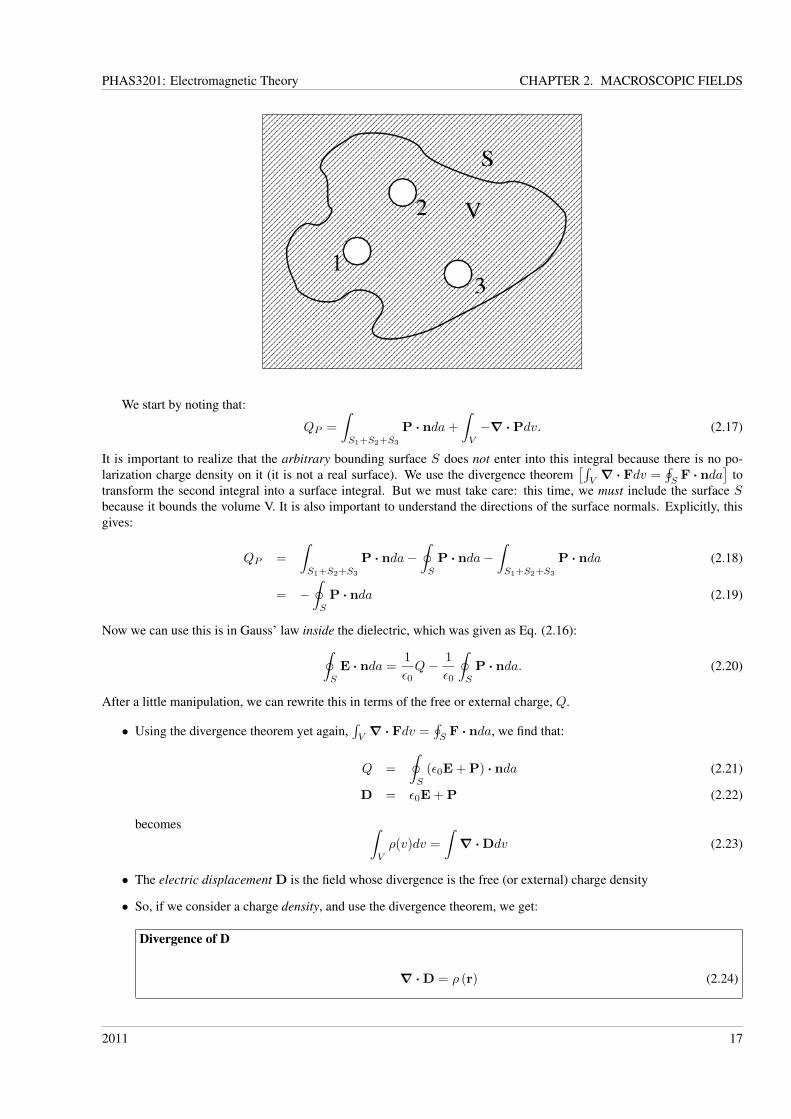
We start by noting that:
QP =
∫S1+S2+S3
P · nda+
∫V
−∇ ·Pdv. (2.17)
It is important to realize that the arbitrary bounding surface S does not enter into this integral because there is no po-larization charge density on it (it is not a real surface). We use the divergence theorem
[∫V∇ · Fdv =
∮SF · nda
]to
transform the second integral into a surface integral. But we must take care: this time, we must include the surface Sbecause it bounds the volume V. It is also important to understand the directions of the surface normals. Explicitly, thisgives:
QP =
∫S1+S2+S3
P · nda−∮S
P · nda−∫S1+S2+S3
P · nda (2.18)
= −∮S
P · nda (2.19)
Now we can use this is in Gauss’ law inside the dielectric, which was given as Eq. (2.16):∮S
E · nda =1
ε0Q− 1
ε0
∮S
P · nda. (2.20)
After a little manipulation, we can rewrite this in terms of the free or external charge, Q.
• Using the divergence theorem yet again,∫V∇ · Fdv =
∮SF · nda, we find that:
Q =
∮S
(ε0E + P) · nda (2.21)
D = ε0E + P (2.22)
becomes ∫V
ρ(v)dv =
∫∇ ·Ddv (2.23)
• The electric displacement D is the field whose divergence is the free (or external) charge density
• So, if we consider a charge density, and use the divergence theorem, we get:
Divergence of D
∇ ·D = ρ (r) (2.24)
2011 17
PHAS3201: Electromagnetic Theory CHAPTER 2. MACROSCOPIC FIELDS
External Charge
• We have talked about free or external charge (as opposed to the bound charge)
• With a dielectric, the difference is clear
• Charge added from outside (external charge) is different to polarization charge
• But it is not free to move
• For a conductor, charge is free to move around
• It is important to be aware of the difference between charge added and charge already present
• In general, the polarization P is a function of the material and the external field E
• We write P = ε0χeE in linear, isotropic, homogeneous media
• In these media, as χe (the electric susceptibility) is constant:
D = ε0E + ε0χeE = εE (2.25)
• We call ε = ε0(1 + χe) the permittivity, and ε/ε0 the relative permittivity or dielectric constant
• Linear: P depends linearly on E
• Homogeneous: χe does not vary with position
• Isotropic: P and E are parallel
[Non-examinable material] [It is important to realize that a sufficiently strong electric field can break apart the chargesin a material which form the microscopic dipoles. At this point, called dielectric breakdown, all approximations discussedto this point are invalid. For air, whose dielectric constant is 1.0006, the maximum field sustainable without breakdown isaround 3× 10⁶ V/m.
The reason that we refer to an isotropic dielectric for the relation P = ε0χe (E)E is that it implies that the polarizationhas the same direction as the external field. This is a good approximation for most media, but it is necessary in some mediato replace this with a tensor relationship, where the two vectors are not in the same direction. This type of behaviour ismore common in magnetic materials, which we will come to.]
Energy Density
• What is the energy density of an electric field?
• We will consider this in two ways:
1. Charge flowing into a capacitor;
2. Adding a small charge to a field.
• The final result is the same:
Energy Density of an Electric Field
U =1
2D ·E (2.26)
Considering a capacitor first, we assume that it is in the process of being charged. If we start with the expression forpower (which is rate of change of energy with time) for a current I(t) flowing at a voltage V (t) at time t, P (t) = V (t)I(t).Then the energy is:
W =
∫P (t)dt =
∫V (t)I(t)dt =
∫Q(t)
C
dQ
dtdt =
1
2
Q2
C(2.27)
2011 18
PHAS3201: Electromagnetic Theory CHAPTER 2. MACROSCOPIC FIELDS
For a parallel plate capacitor with plates of area A separated by a distance d, we know that the capacitance is given byC = εA
d . Using V = Q/C, we find that the electric field can be written:
E =V
d=
Q
Cd=
Qd
εAd=
Q
εA. (2.28)
Of course, as D = εE, we find that D = QA . So the energy density is given by:
U =W
Ad=
1
2
Q2
CAd
=1
2
Q2
εA2
=1
2D ·E (2.29)
Another (more general) way to reach the same formula is to consider the work done bringing a charge from infinity tothe point where the energy density is required. We know that the energy of a point charge, q, in a potential φ is W = qφ.This can be generalized for a charge distribution given by the charge density ρ(r):
W =
∫V
ρφdv. (2.30)
Now, what would be change in electrostatic energy when adding a small amount of charge, δρ? We use our recentresult for Gauss’ theorem,∇ ·D = ρ:
δW =
∫V
δρφdv (2.31)
δρ = ∇ · δD (2.32)φ (∇ ·D) = ∇ · (φD)−D · (∇φ) (2.33)
δW =
∫V
∇ · (φδD)− δD · ∇φdv (2.34)
δW =
∫S
φδD · nda−∫V
δD · ∇φdv, (2.35)
where we have used the divergence theorem on the first part of the integral in the final line. But we know that E = −∇φ,and we can notice that the first term will fall off rapidly with distance (D with 1/r2 and φ with 1/r). This means that wecan write overall, as the volume being integrated tends to infinity:
δW =
∫V
δD ·Edv (2.36)
Now, if we assume a linear, dielectric medium, we know that D = εE, and we can integrate over the field going from 0to D:
W =
∫ D
0
δW =
∫ D
0
∫V
δD ·Edv (2.37)
We can write:
W =1
2
∫ E
0
∫V
εδ(E2)dv =
1
2
∫V
εE2dv (2.38)
This of course gives us the result we derived above, namely U = E ·D/2.
2011 19
PHAS3201: Electromagnetic Theory CHAPTER 2. MACROSCOPIC FIELDS
2.3 Magnetic Fields RevisionAn important point to note as we start the area of magnetic fields is that this is where the essential link between elec-tric fields and magnetic fields (leading to the unified area of electromagnetism) becomes apparent. Thus far we haveconsidered electrostatics only.
• The magnetic field at r2 due to a circuit at r1, in both integral and differential forms:
Biot-Savart Field Law
B (r2) =µ0
4πI1
∮1
dl1 × r12
|r12|3(2.39)
dB (r2) =µ0
4πI1dl1 × r12
|r12|3(2.40)
• Note that this is empiricially derived.
• For a current density, we find:
B (r2) =µ0
4π
∫V
J (r1)× r12
|r12|3dv1 (2.41)
• This implies that∇2 ·B = 0, which indicates a lack of magnetic monopoles.
We can show the last statement using the mathematical identity for∇ · (F×G) = (∇× F) ·G− (∇×G) · F:
∇2 ·B =µ0
4π
∫V
∇2 ·(J (r1)× r12
|r12|3
)dv1 (2.42)
=µ0
4π
∫V
−J (r1) ·(∇2 ×
r12
|r12|3
)dv1, (2.43)
where, since we are taking the divergence at point r2, the term involving∇2 × J (r1) is zero. But now we can use twoidentities:
1. ∇ (1/r12) = r12/ |r12|3
2. ∇× (∇φ) = 0
This shows that the integral on the right-hand size of equation (2.43) is zero, and hence there are no magnetic monopoles(though note that we started from just this assumption: that the magnetic field arises from the line integral around acircuit!).
• The original, integral form of Ampère’s Law is: ∮C
B · dl = µ0I, (2.44)
where the current is that flowing through the area enclosed by the path.
• The differential form comes from writing I =∫SJ · nda
∇×B = µ0J (2.45)
• But we have to account for time-varying E:
Ampère-Maxwell Law
∇×B = µ0J + µ0ε0∂E
∂t(2.46)
2011 20
PHAS3201: Electromagnetic Theory CHAPTER 2. MACROSCOPIC FIELDS
We can understand why this is incomplete by considering a capacitor being charged with a constant current, I. UsingAmpère’s law (in original form) we see: ∮
B · dl = µ0
∫S
J · nda (2.47)
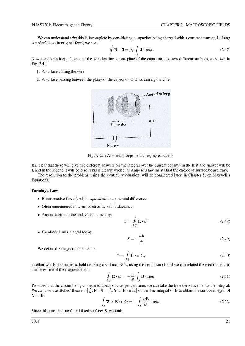
Now consider a loop, C, around the wire leading to one plate of the capacitor, and two different surfaces, as shown inFig. 2.4:
1. A surface cutting the wire
2. A surface passing between the plates of the capacitor, and not cutting the wire
Figure 2.4: Ampèrian loops on a charging capacitor.
It is clear that these will give two different answers for the integral over the current density: in the first, the answer will beI, and in the second it will be zero. This is clearly wrong, as Ampère’s law insists that the choice of surface be arbitrary.
The resolution to the problem, using the continuity equation, will be considered later, in Chapter 5, on Maxwell’sEquations.
Faraday’s Law
• Electromotive force (emf) is equivalent to a potential difference
• Often encountered in terms of circuits, with inductance
• Around a circuit, the emf, E , is defined by:
E =
∮C
E · dl (2.48)
• Faraday’s Law (integral form):
E = −dΦ
dt(2.49)
We define the magnetic flux, Φ, as:
Φ =
∫S
B · nda, (2.50)
in other words the magnetic field crossing a surface. Now, using the definition of emf we can related the electric field tothe derivative of the magnetic field: ∮
C
E · dl = − d
dt
∫S
B · nda. (2.51)
Provided that the circuit being considered does not change with time, we can take the time derivative inside the integral.We can also use Stokes’ theorem
[∮CF · dl =
∫S∇× F · nda
]on the line integral of E to obtain the surface integral of
∇×E: ∫s
∇×E · nda = −∫S
∂B
∂t· nda. (2.52)
Since this must be true for all fixed surfaces S, we find:
2011 21
PHAS3201: Electromagnetic Theory CHAPTER 2. MACROSCOPIC FIELDS
•
The differential form of Faraday’s Law:
∇×E = −∂B∂t
(2.53)
• When the magnetic field is static, this reduces to the conservative field E,∇×E = 0.
• Notice the minus sign: Lenz’s law states that any induced magnetic field opposes the change in flux that induced it
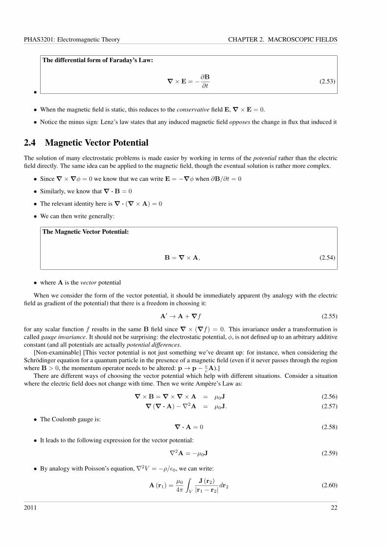
2.4 Magnetic Vector PotentialThe solution of many electrostatic problems is made easier by working in terms of the potential rather than the electricfield directly. The same idea can be applied to the magnetic field, though the eventual solution is rather more complex.
• Since∇×∇φ = 0 we know that we can write E = −∇φ when ∂B/∂t = 0
• Similarly, we know that∇ ·B = 0
• The relevant identity here is∇ · (∇×A) = 0
• We can then write generally:
The Magnetic Vector Potential:
B =∇×A, (2.54)
• where A is the vector potential
When we consider the form of the vector potential, it should be immediately apparent (by analogy with the electricfield as gradient of the potential) that there is a freedom in choosing it:
A′ → A +∇f (2.55)
for any scalar function f results in the same B field since ∇ × (∇f) = 0. This invariance under a transformation iscalled gauge invariance. It should not be surprising: the electrostatic potential, φ, is not defined up to an arbitrary additiveconstant (and all potentials are actually potential differences.
[Non-examinable] [This vector potential is not just something we’ve dreamt up: for instance, when considering theSchrödinger equation for a quantum particle in the presence of a magnetic field (even if it never passes through the regionwhere B > 0, the momentum operator needs to be altered: p→ p− e
cA).]There are different ways of choosing the vector potential which help with different situations. Consider a situation
where the electric field does not change with time. Then we write Ampère’s Law as:
∇×B =∇×∇×A = µ0J (2.56)∇ (∇ ·A)−∇2A = µ0J. (2.57)
• The Coulomb gauge is:∇ ·A = 0 (2.58)
• It leads to the following expression for the vector potential:
∇2A = −µ0J (2.59)
• By analogy with Poisson’s equation,∇2V = −ρ/ε0, we can write:
A (r1) =µ0
4π
∫V
J (r2)
|r1 − r2|dr2 (2.60)
2011 22
PHAS3201: Electromagnetic Theory CHAPTER 2. MACROSCOPIC FIELDS
• The current density determines the vector potential
• There are other choices of gauge, for instance, the Lorentz gauge is∇ ·A = −µoε0 (∂V/∂t).
• Gauge invariance is a more general phenomenon
• Solving for vector potential is (generally) harder than solving for the electrostatic potential
• The electric field can no longer be expressed as the gradient of a scalar potential if there is a time-varying B field:
E(t) = −∇φ− ∂A
∂t(2.61)
This last change can be seen rather easily. Consider the Maxwell equation for the curl of the electric field:
∇×E = −∂B∂t
(2.62)
and substitute in the form of B =∇×A:
∇×E +∂
∂t∇×A = 0 (2.63)
The vector E + ∂A/∂t has zero curl. We know from identities that it can be written as a gradient of a scalar:
E +∂A
∂t= −∇φ (2.64)
So, rearranging, we find that E = −∇φ− ∂A/∂t
2.5 Magnetic IntensityAs we saw with the electric field, E, the introduction of a medium other than vacuum results in changes to Maxwell’sequations. These changes can be handled by using an alternative field which includes the effects of the medium implicitly.We will now do the same for magnetic fields. A word of caution: non-linear magnetic media are much more commonthan non-linear electric media; we will deal with these rather interesting materials in Chapter 4 on Ferromagnetism.
• Magnetization
• We introduced the polarization of a dielectric material, P ∝ E
• Similarly, we introduce a quantity, proportional to the magnetic induction B
• This is the magnetization, M
• It describes the response of a material to the magnetic induction
• Electrons can be modelled as moving in loops around atoms: we can use the magnetic dipole to model the response
Let us consider the vector potential at a point r1 due to a small volume of magnetised material at a point r2 (we willsee later that this is given by the expression below). This small volume will have magnetic moment ∆m = M (r2) δV2.Then we can write:
A (r1) =µ0
4π
∫V
∆m× r12
|r12|3(2.65)
=µ0
4π
∫V
M (r2)× r12
|r12|3dV2 (2.66)
=µ0
4π
∫V
M (r2)×∇21
r12dV2, (2.67)
2011 23
PHAS3201: Electromagnetic Theory CHAPTER 2. MACROSCOPIC FIELDS
where we’ve used a standard result to get from Eq. (2.66) to Eq. (2.67). Now we use the expansion of ∇ × (φF), withF = M and φ = 1
r12to write:
F×∇φ = φ∇× F−∇× (φF) (2.68)
A (r1) =µ0
4π
∫V
{∇2 ×M (r2)
r12−∇2 ×
(M (r2)
r12
)}dV2 (2.69)
Now we use the theorem∫V∇× FdV =
∫Sn× Fda to write:
A (r1) =µ0
4π
∫V
∇2 ×M (r2)
r12dV2 −
µ0
4π
∫S
n×M (r2)
r12da2 (2.70)
=µ0
4π
∫V
∇2 ×M (r2)
r12dV2 +
µ0
4π
∫S
M× n (r2)
r12da2 (2.71)
• This then leads us to the magnetization current densities:
• We formally define:
JM = ∇×M (2.72)jM = M× n (2.73)
• JM is the volume magnetization current density
• jM is the surface magnetization current density
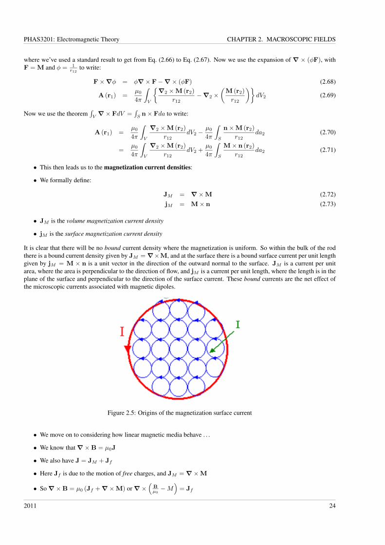
It is clear that there will be no bound current density where the magnetization is uniform. So within the bulk of the rodthere is a bound current density given by JM =∇×M, and at the surface there is a bound surface current per unit lengthgiven by jM = M × n is a unit vector in the direction of the outward normal to the surface. JM is a current per unitarea, where the area is perpendicular to the direction of flow, and jM is a current per unit length, where the length is in theplane of the surface and perpendicular to the direction of the surface current. These bound currents are the net effect ofthe microscopic currents associated with magnetic dipoles.
Figure 2.5: Origins of the magnetization surface current
• We move on to considering how linear magnetic media behave . . .
• We know that∇×B = µ0J
• We also have J = JM + Jf
• Here Jf is due to the motion of free charges, and JM =∇×M
• So∇×B = µ0 (Jf +∇×M) or∇×(
Bµ0−M
)= Jf
2011 24
PHAS3201: Electromagnetic Theory CHAPTER 2. MACROSCOPIC FIELDS
• We then define H, the magnetic intensity, as
Magnetic Intensity
H =B
µ0−M (2.74)
• This yields∇×H = Jf
The magnetic intensity serves a similar purpose to the electric displacement, in accounting for the response of themedium as well as the magnetic induction. We can rewrite this, using Stokes’ theorem:∫
S
∇×H · nda =
∫S
Jf · nda (2.75)∮C
H · dl =
∫S
Jf · nda (= If ) (2.76)
This tells us that the integral of the intensity along a closed loop is equal to the current flowing across the surface definedby that loop. It also gives the units as amperes per metre (the same units as the magnetization).
It is important to note that the three quantities that we have defined so far (the magnetic induction, B, the magneti-zation, M and the magnetic intensity, H) are not necessarily parallel; this will be important when considering ferromag-netism in particular.
Magnetic Susceptibility
• For a linear, isotropic material, we assert (based on experimental observations):
M = χmH (2.77)
where χm is the magnetic susceptibility
• We can write B = µ0 (1 + χm)H
• If χm > 0 we have a paramagnetic material
• If χm < 0 we have a diamagnetic material
• Note that χm can depend on temperature, but is generally small for these materials (less than 10−5)
2.6 Interfaces and Boundary Conditions• Understanding how the different field vectors change at interfaces is important
• We need to consider both medium/vacuum and medium/medium interfaces
• We will consider the electric and magnetic fields in two groups:
– D and B together
– E and H together
• We want to know what is conserved
Normal components
• First notice that we can write similar equations for
D and B:
∇ ·D = ρf
∇ ·B = 0
2011 25
PHAS3201: Electromagnetic Theory CHAPTER 2. MACROSCOPIC FIELDS
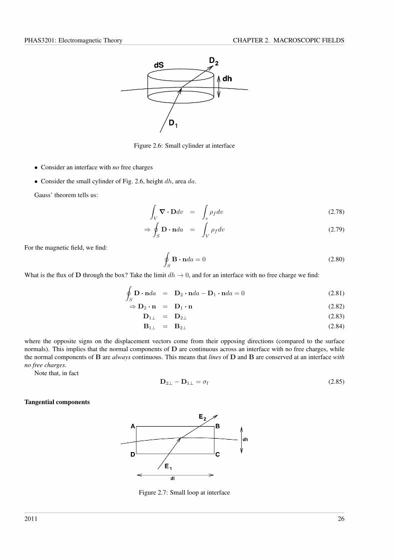
Figure 2.6: Small cylinder at interface
• Consider an interface with no free charges
• Consider the small cylinder of Fig. 2.6, height dh, area da.
Gauss’ theorem tells us: ∫V
∇ ·Ddv =
∫v
ρfdv (2.78)
⇒∮S
D · nda =
∫V
ρfdv (2.79)
For the magnetic field, we find: ∮S
B · nda = 0 (2.80)
What is the flux of D through the box? Take the limit dh→ 0, and for an interface with no free charge we find:∮S
D · nda = D2 · nda−D1 · nda = 0 (2.81)
⇒ D2 · n = D1 · n (2.82)D1⊥ = D2⊥ (2.83)B1⊥ = B2⊥ (2.84)
where the opposite signs on the displacement vectors come from their opposing directions (compared to the surfacenormals). This implies that the normal components of D are continuous across an interface with no free charges, whilethe normal components of B are always continuous. This means that lines of D and B are conserved at an interface withno free charges.
Note that, in factD2⊥ −D1⊥ = σf (2.85)
Tangential components
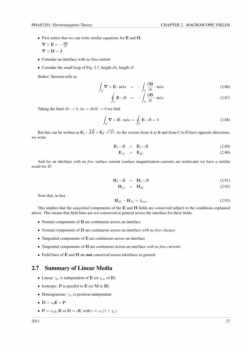
Figure 2.7: Small loop at interface
2011 26
PHAS3201: Electromagnetic Theory CHAPTER 2. MACROSCOPIC FIELDS
• First notice that we can write similar equations for E and H:
∇×E = −∂B∂t∇×H = J
• Consider an interface with no free current
• Consider the small loop of Fig. 2.7, height dh, length dl.
Stokes’ theorem tells us ∫S
∇×E · nda = −∫S
∂B
∂t· nda (2.86)∮
C
E · dl = −∫S
∂B
∂t· nda (2.87)
Taking the limit dh→ 0, da = dldh→ 0 we find:∫S
∇×E · nda =
∮C
E · dl = 0 (2.88)
But this can be written as E1 ·−−→AB + E2 ·
−−→CD. As the vectors from A to B and from C to D have opposite directions,
we write:
E1 · dl = E2 · dl (2.89)E1‖ = E2‖ (2.90)
And for an interface with no free surface current (surface magnetization currents are irrelevant) we have a similarresult for H:
H1 · dl = H2 · dl (2.91)H1‖ = H2‖ (2.92)
Note that, in factH2‖ −H1‖ = Ifenc (2.93)
This implies that the tangential components of the E and H fields are conserved subject to the conditions explainedabove. This means that field lines are not conserved in general across the interface for these fields.
• Normal components of B are continuous across an interface
• Normal components of D are continuous across an interface with no free charges
• Tangential components of E are continuous across an interface
• Tangential components of H are continuous across an interface with no free currents
• Field lines of E and H are not conserved across interfaces in general
2.7 Summary of Linear Media• Linear: χe is independent of E (or χm of B)
• Isotropic: P is parallel to E (or M to H)
• Homogeneous: χe is position independent
• D = ε0E + P
• P = ε0χeE so D = εE, with ε = ε0 (1 + χe)
2011 27
PHAS3201: Electromagnetic Theory CHAPTER 2. MACROSCOPIC FIELDS
• ∇ ·D = ρf
• H = B/µ0 −M
• M = χmH so B = µ0µrH with µr = 1 + χm
• ∇×H = Jf
• continuous across an interface:
– B⊥
– D⊥ when no free charges
– E‖
– H‖ when no free currents
2011 28
PHAS3201: Electromagnetic Theory CHAPTER 3. ATOMIC MECHANISMS
Chapter 3
Atomic Mechanisms
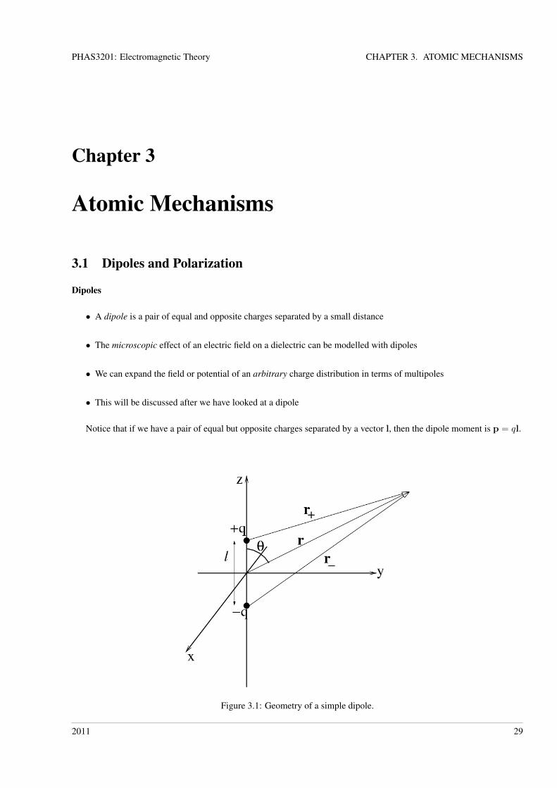
3.1 Dipoles and Polarization
Dipoles
• A dipole is a pair of equal and opposite charges separated by a small distance
• The microscopic effect of an electric field on a dielectric can be modelled with dipoles
• We can expand the field or potential of an arbitrary charge distribution in terms of multipoles
• This will be discussed after we have looked at a dipole
Notice that if we have a pair of equal but opposite charges separated by a vector l, then the dipole moment is p = ql.
Figure 3.1: Geometry of a simple dipole.
2011 29
PHAS3201: Electromagnetic Theory CHAPTER 3. ATOMIC MECHANISMS
Dipole Geometry
E (r) =q
4πε0
(r+
r2+
− r−r2−
)(3.1)
V (r) =q
4πε0
(1
r+− 1
r−
)(3.2)
r+ = r− l/2 (3.3)r− = r + l/2 (3.4)
• V (r) is easier to work with than E(r)
What is the electric field at a point r due to a dipole (length l) at the origin, oriented along the z axis? (Note thatwe have decided to put the dipole at the origin, and chosen an easy orientation; these can be generalized without muchdifficulty). Define the vectors involved:
r+ = r− l
2(3.5)
r− = r +l
2(3.6)
We need to know the magnitude of r+ and r−, so using Eqs. (3.5) and (3.6), we find
|r+| =√r+ · r+ (3.7)
r+ · r+ = r2 − rl cos θ +l2
4(3.8)
= r2
(1− l
rcos θ +
l2
4r2
)(3.9)
|r+| = r
√1− l
rcos θ +
l2
4r2(3.10)
|r−| = r
√1 +
l
rcos θ +
l2
4r2(3.11)
(3.12)
We can now write down 1/ |r+| and 1/ |r−| and expand them to first order in l/r:
1
|r+|=
1
r
(1− l
rcos θ +
l2
4r2
)− 12
(3.13)
' 1
r
(1 +
l
2rcos θ
)(3.14)
1
|r−|' 1
r
(1− l
2rcos θ
), (3.15)
where we have used (1 + δ)n ' 1 + nδ to first order in δ. Note that this is only valid when r � l. Now,
1
|r+|− 1
|r−|=
l
r2cos θ, (3.16)
so the potential is given by:
Dipole Potential:
V (r) =ql cos θ
4πε0r2=
p · r4πε0r2
, (3.17)
where p is the dipole moment, defined as:
p = ql (3.18)
p =
∫V
rρ (r) dv, (3.19)
2011 30
PHAS3201: Electromagnetic Theory CHAPTER 3. ATOMIC MECHANISMS
where the second form is for the dipole moment of a charge density in a small volume V . Now that we have the potential,we can calculate the field. Notice that we have naturally ended up working in spherical polar coordinates (with θ definedas the angle from the z-axis), and that there is no dependence on φ.
[The following brief discussion of multipole expansion follows Griffiths pp.149-150, and is not directly exam-inable; however, it is extremely useful to understand, and is well within the capability of students.]
In outline, we start by considering the potential at a point r due to an arbitrary charge distribution, ρ(r′). This can bewritten as:
V (r) =1
4πε0
∫ρ(r′)
|R|dr′, (3.20)
where R = r− r′. In order to make this simpler, we need to rewrite |R| in terms of r and r′. The magnitude of R can befound from a dot product:
R ·R = (r− r′) · (r− r′) (3.21)= r2 + (r′)2 − 2rr′ cos θ, (3.22)
where θ is the angle between r and r′. By taking a factor of r2 outside, we see that we can write:
R2 = r2
(1 +
(r′
r
)2
− 2
(r′
r
)cos θ
)(3.23)
⇒ R = r√
1 + ε (3.24)
ε =
(r′
r
)((r′
r
)− 2 cos θ
)(3.25)
So we can expand 1/R using the binomial expansion; it is important to note that we will not make any approximation,and inherently carry the full expansion with us (though it will not be shown).
1
R=
1
r(1 + ε)−1/2 =
1
r
[1− 1
2ε+
3
8ε2 − 5
16ε3 + . . .
](3.26)
=1
r
[1− 1
2
(r′
r
)((r′
r
)− 2 cos θ
)+
3
8
(r′
r
)2((r′
r
)− 2 cos θ
)2
+ . . .
](3.27)
Now gathering terms in(r′
r
), this can be written:
1
R=
1
r
[1 +
(r′
r
)cos θ +
(r′
r
)23 cos2 θ − 1
2+
(r′
r
)35 cos3 θ − 3 cos θ
2+ . . .
](3.28)
=1
r
∞∑0
(r′
r
)nPn(cos θ), (3.29)
where Pn(cos θ) are the Legendre polynomials. Substituting this expression into Eq. (3.20) for the potential, we find:
V (r) =1
4πε0
[1
r
∫ρ(r′)dv′ +
1
r2
∫r′ cos θρ(r′)dv′ +
1
r3
∫(r′)2(
3
2cos θ − 1
2)ρ(r′)dv′ + . . .
](3.30)
=1
4πε0
∞∑0
1
rn+1
∫(r′)nPn(cos θ)ρ(r′)dv′ (3.31)
This shows that for large distances, an arbitrary charge distribution behaves approximately like the total charge (thefirst term, which falls off with 1/r, is known as the monopole term). Other terms can be brought in to improve the
2011 31
PHAS3201: Electromagnetic Theory CHAPTER 3. ATOMIC MECHANISMS
approximation (and will be important at shorter distances): the dipole term scales with 1/r2, the quadrupole term scaleswith 1/r3, the octopole term with 1/r4 etc.
[End of multipole discussion]
Starting from the potential we just derived, and working in spherical polar coordinates, we can write:
E (r) = −∇V = −r∂V∂r− θ 1
r
∂V
∂θ− φ 1
r sin θ
∂V
∂φ(3.32)
∂V
∂r= −2
ql cos θ
4πε0r3(3.33)
∂V
∂θ= − ql sin θ
4πε0r2(3.34)
∂V
∂φ= 0 (3.35)
Dipole Field and Potential
Er(r, θ, φ) =ql cos θ
2πε0r3(3.36)
Eθ(r, θ, φ) =ql sin θ
4πε0r3(3.37)
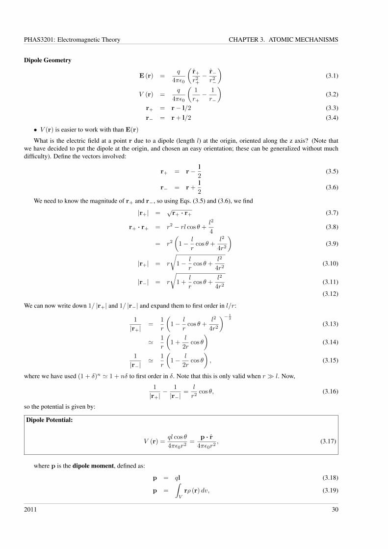
• The potential is zero along the centre line (x-y plane)
• The field decays as 1/r3, potential as 1/r2
• As always, the electric field is always perpendicular to equipotentials
Figure 3.2: Electric field and equipotentials for a dipole.
• Ultimately, we want to understand the response of matter to applied fields
• We looked at the potential of an arbitrary charge distribution
• Expanding 1/R we made the multipole expansion
• We then derived the potential & electric field for a dipole
• The potential falls off as 1/r2, the field as 1/r3
2011 32
PHAS3201: Electromagnetic Theory CHAPTER 3. ATOMIC MECHANISMS
Microscopic Dipoles
• Dielectrics have no free charges
• Atoms consist of nuclei and electrons which respond to an applied field
• Positive charge moves with field, negative against it
• But the displacement is limited by a restoring force
• This results in a neutral material with a net dipole
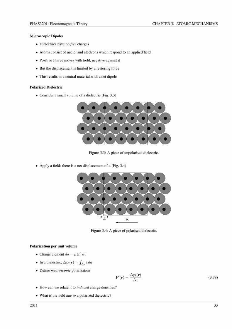
Polarized Dielectric
• Consider a small volume of a dielectric (Fig. 3.3)
Figure 3.3: A piece of unpolarised dielectric.
• Apply a field: there is a net displacement of a (Fig. 3.4)
Figure 3.4: A piece of polarised dielectric.
Polarization per unit volume
• Charge element dq = ρ (r) dv
• In a dielectric, ∆p (r) =∫
∆vrdq
• Define macroscopic polarization
P (r) =∆p (r)
∆v(3.38)
• How can we relate it to induced charge densities?
• What is the field due to a polarized dielectric?
2011 33
PHAS3201: Electromagnetic Theory CHAPTER 3. ATOMIC MECHANISMS
There are two approaches: one simple (as found in Grant & Phillips), and one more rigorous. We consider the simpleone first, then expand to the rigorous one.
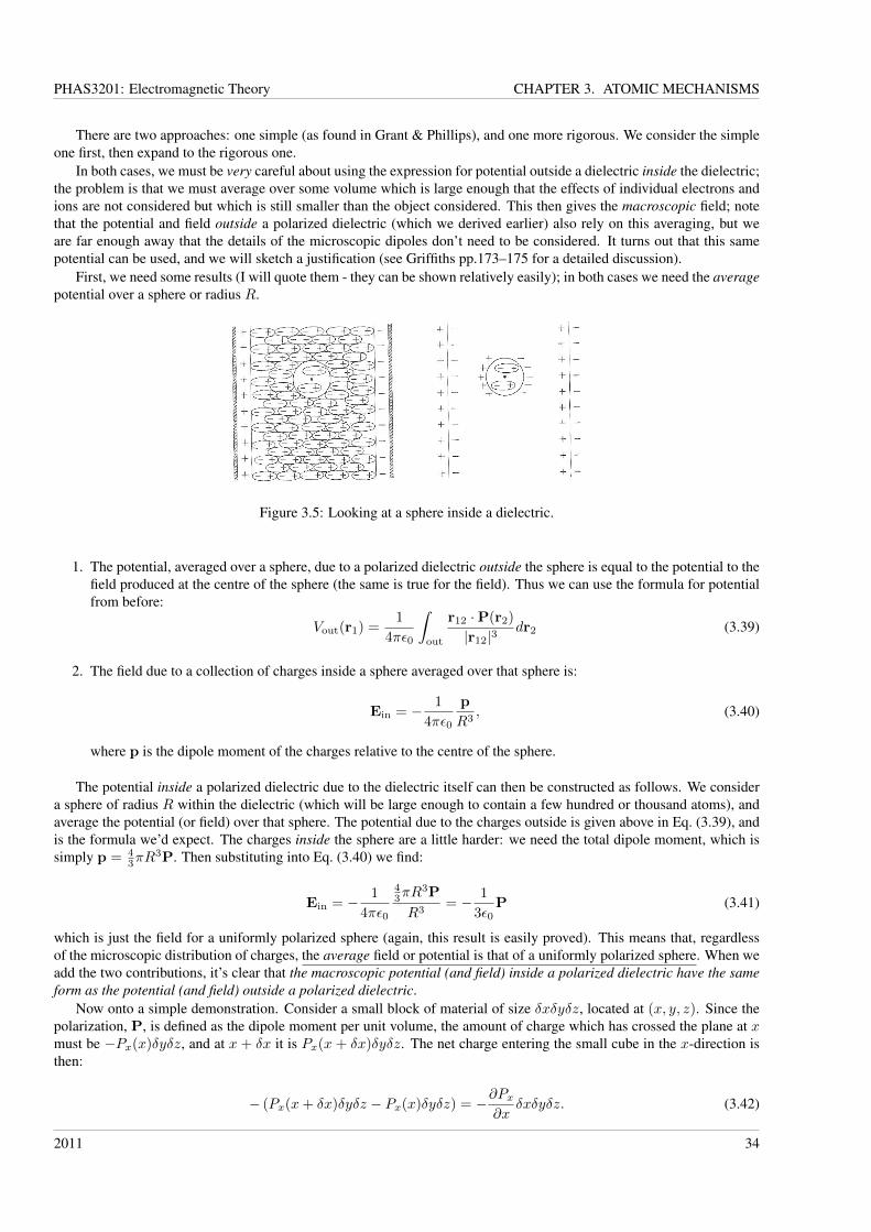
In both cases, we must be very careful about using the expression for potential outside a dielectric inside the dielectric;the problem is that we must average over some volume which is large enough that the effects of individual electrons andions are not considered but which is still smaller than the object considered. This then gives the macroscopic field; notethat the potential and field outside a polarized dielectric (which we derived earlier) also rely on this averaging, but weare far enough away that the details of the microscopic dipoles don’t need to be considered. It turns out that this samepotential can be used, and we will sketch a justification (see Griffiths pp.173–175 for a detailed discussion).
First, we need some results (I will quote them - they can be shown relatively easily); in both cases we need the averagepotential over a sphere or radius R.
Figure 3.5: Looking at a sphere inside a dielectric.
1. The potential, averaged over a sphere, due to a polarized dielectric outside the sphere is equal to the potential to thefield produced at the centre of the sphere (the same is true for the field). Thus we can use the formula for potentialfrom before:
Vout(r1) =1
4πε0
∫out
r12 ·P(r2)
|r12|3dr2 (3.39)
2. The field due to a collection of charges inside a sphere averaged over that sphere is:
Ein = − 1
4πε0
p
R3, (3.40)
where p is the dipole moment of the charges relative to the centre of the sphere.
The potential inside a polarized dielectric due to the dielectric itself can then be constructed as follows. We considera sphere of radius R within the dielectric (which will be large enough to contain a few hundred or thousand atoms), andaverage the potential (or field) over that sphere. The potential due to the charges outside is given above in Eq. (3.39), andis the formula we’d expect. The charges inside the sphere are a little harder: we need the total dipole moment, which issimply p = 4
3πR3P. Then substituting into Eq. (3.40) we find:
Ein = − 1
4πε0
43πR
3P
R3= − 1
3ε0P (3.41)
which is just the field for a uniformly polarized sphere (again, this result is easily proved). This means that, regardlessof the microscopic distribution of charges, the average field or potential is that of a uniformly polarized sphere. When weadd the two contributions, it’s clear that the macroscopic potential (and field) inside a polarized dielectric have the sameform as the potential (and field) outside a polarized dielectric.
Now onto a simple demonstration. Consider a small block of material of size δxδyδz, located at (x, y, z). Since thepolarization, P, is defined as the dipole moment per unit volume, the amount of charge which has crossed the plane at xmust be −Px(x)δyδz, and at x + δx it is Px(x + δx)δyδz. The net charge entering the small cube in the x-direction isthen:
− (Px(x+ δx)δyδz − Px(x)δyδz) = −∂Px∂x
δxδyδz. (3.42)
2011 34
PHAS3201: Electromagnetic Theory CHAPTER 3. ATOMIC MECHANISMS
We can write similar equations for the y and z directions, and find that the total charge is given by:(−∂Px∂x− ∂Py
∂y− ∂Pz
∂z
)δxδyδz (3.43)
If we divide this charge by the volume element δxδyδz then we find an effective polarization charge density:
ρP = −∇ ·P. (3.44)
In uniform, bulk dielectrics this will tend to zero as the number of charges entering and leaving will be the same; nearsurfaces or areas where the density varies rapidly then charges accumulate. These two effects are seen more clearly next.
[NOTE This derivation has already appeared in Section II on Macroscopic Fields, but it’s repeated here for complete-ness; it may well not be repeated in the lectures.]
For the more rigorous demonstration, we start by finding the potential at a point r due to a small volume of polarizedmaterial at a point r′. We will then integrate this over the entire piece of dielectric material. We write, using Eq. (3.17):
∆φ (r) =∆p (r′) · (r− r′)
4πε0 |r− r′|3(3.45)
=∆v′P (r′) · (r− r′)
4πε0 |r− r′|3(3.46)
When we take the limit ∆v → 0 and sum over the elements, we get an expression for the total potential:
φ (r) =
∫V
dv′P (r′) · (r− r′)
4πε0 |r− r′|3(3.47)
We use the gradient of 1/ |r− r′| to transform this:
φ (r) =1
4πε0
∫V
P (r′) · ∇′(
1
|r− r′|
)dv′ (3.48)
Using the formula for∇ · (φF) from the Mathematical Identities, and rearranging (we want F · ∇φ) we can write:
φ (r) =1
4πε0
∫V
{∇ ·
(P (r′)
|r− r′|
)− 1
|r− r′|∇ ·P (r′)
}dv′ (3.49)
Finally, we use the divergence theorem on the first term to give the potential outside a polarized dielectric object:
φ (r) =1
4πε0
∮S
P (r′) · n|r− r′|
da′ +1
4πε0
∫V
−∇ ·P (r′)
|r− r′|dv′ (3.50)
Polarization Charge Densities
• The surface polarization charge density is defined:
σP = P · n (3.51)
• The volume polarization charge density is defined:
ρP = −∇ ·P (3.52)
• We can write the potential as:
φ (r) =1
4πε0
(∮S
σP|r− r′|
da′ +
∫V
ρP|r− r′|
dv′)
(3.53)
=1
4πε0
∫dqP|r− r′|
(3.54)
2011 35
PHAS3201: Electromagnetic Theory CHAPTER 3. ATOMIC MECHANISMS
Does this mean that the dielectric is now charged? To understand this, consider a polarized dielectric, with volume V0.We must consider the outside surface S0, and its associated polarization charge density. Using the divergence theorem wecan write:
QP =
∫V0
ρP dv +
∮S0
σP da (3.55)
=
∫V0
−∇ ·Pdv +
∮S0
P · nda (3.56)
= −∮S0
P · nda+
∮S0
P · nda = 0. (3.57)
So the overall dielectric is electrically neutral (which we assumed at the start). However, the field can be non-zero: inparticular, if there is an applied external field inducing the polarization, then the dielectric itself will affect that field. Forcompleteness, note that we can write:
E (r) =1
4πε0
(∮S
σP (r− r′)
|r− r′|3da′ +
∫V
ρP (r− r′)
|r− r′|3dv′
)(3.58)
• Polarization arises from alignment of microscopic dipoles
• These give surface and volume polarization charge densities
• We looked at potential inside and outside dielectric
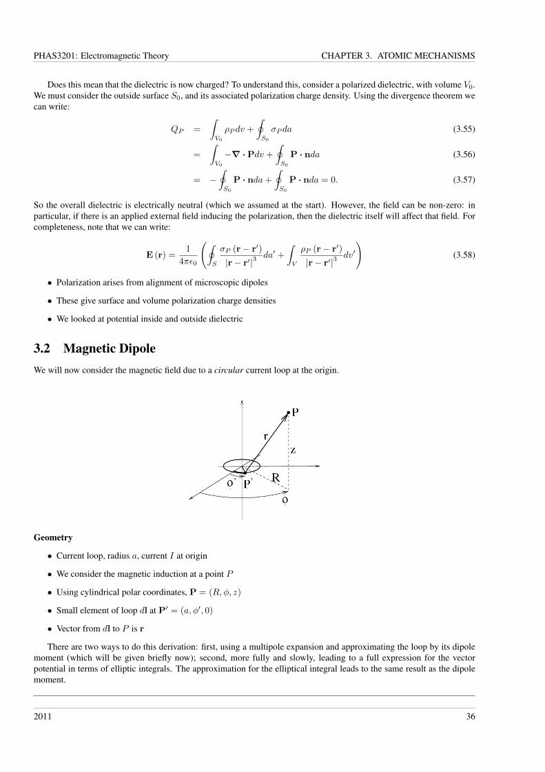
3.2 Magnetic DipoleWe will now consider the magnetic field due to a circular current loop at the origin.
Geometry
• Current loop, radius a, current I at origin
• We consider the magnetic induction at a point P
• Using cylindrical polar coordinates, P = (R,φ, z)
• Small element of loop dl at P′ = (a, φ′, 0)
• Vector from dl to P is r
There are two ways to do this derivation: first, using a multipole expansion and approximating the loop by its dipolemoment (which will be given briefly now); second, more fully and slowly, leading to a full expression for the vectorpotential in terms of elliptic integrals. The approximation for the elliptical integral leads to the same result as the dipolemoment.
2011 36
PHAS3201: Electromagnetic Theory CHAPTER 3. ATOMIC MECHANISMS
[Derivation of vector potential for arbitrary current loop]In the Macroscopic Fields part of the course, we showed that, using the Coulomb gauge, the vector potential at a point
r due to a current density J(r) distributed over a volume at r′ could be written:
A(r) =µ0
4π
∫J(r′)
|r− r′|dv′ (3.59)
For a constant current I in an arbitrary loop, with Jdv ⇒ Idl, we can rewrite the volume integral as a line integral.Re-introducing the vector R = r− r′, we write:
A(r) =µ0I
4π
∫dl′
|R|(3.60)
As with the potential of a charge distribution, we now need to write |R| in terms of r and r′. Using Legendre polynomialsagain, and recalling that the angle between r and r′ is θ, we find by substituting into Eq. (3.60) that:
A(r) =µ0I
4π
∞∑0
1
rn+1
∮(r′)nPn(cos θ)dl′ (3.61)
=µ0I
4π
[1
r
∮dl′ +
1
r2
∮r′ cos θdl′ +
1
r3
∮(r′)2
(3
2cos2 θ − 1
2
)+ . . .
](3.62)
Now notice that the first term (the monopole term) is multiplied by a closed loop integral with integrand 1, whichis identically zero (it is not surprising that the monopole term disappears as we started from the assumption that thereare no monopoles). So the first non-zero term in the expansion is a dipole term; we will use the identity
∮r′ cos θdl′ =∮
(r · r′)dl′ = −r×∫da′ to simplify this. Then the dipole term only is:
Adip(r) =µ0I
4πr2
∮r′ cos θdl′ (3.63)
=µ0I
4π
∫da′ × r
r2=µ0
4π
m× r
r2, (3.64)
where m = I∫da′ = Ia is the magnetic dipole moment. This derivation allows a full expansion to be made for an
arbitrary current loop; far from this loop it behaves like a dipole. This vector potential will be seen again below.[End of multipole expansion for arbitrary current loop]
We now return to the derivation of the vector potential for a circular current loop. Let us consider first how to writethe vector for the small element of loop, dl:
dl = dφ′ · a · (− sinφ′i + cosφ′j) (3.65)
Here we’ve used the standard two-dimensional formula for arc length, and projected it onto Cartesian vectors. Note thatwe want the direction of dl to be tangential to the current loop; so at φ′ = 0 it lies along y-axis, at φ′ = π/2 it lies alongthe x-axis but in the opposite direction etc. We’ve basically taken the gradient of the position on the unit circle.
We now consider the magnetic induction due to the current loop. One approach would be to use the Biot-Savart law,and integrate around the current loop, but this quickly becomes very complicated. Instead, we will use the vector potential;this isn’t trivial, but it’s easier, and allows us to get further.
First we notice that we can change Jdv ⇒ Idl for a constant current through the loop.
Vector Potential
• We can write for the vector potential at P (a point, not polarization!):
A (P) =µ0
4π
∫V
J (P′)
|P−P′|dv (3.66)
=µ0I
4π
∮dl
|r|(3.67)
2011 37
PHAS3201: Electromagnetic Theory CHAPTER 3. ATOMIC MECHANISMS
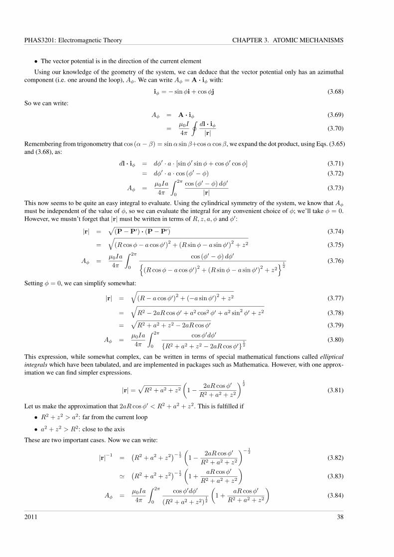
• The vector potential is in the direction of the current element
Using our knowledge of the geometry of the system, we can deduce that the vector potential only has an azimuthalcomponent (i.e. one around the loop), Aφ. We can write Aφ = A · iφ with:
iφ = − sinφi + cosφj (3.68)
So we can write:
Aφ = A · iφ (3.69)
=µ0I
4π
∮dl · iφ|r|
(3.70)
Remembering from trigonometry that cos (α− β) = sinα sinβ+cosα cosβ, we expand the dot product, using Eqs. (3.65)and (3.68), as:
dl · iφ = dφ′ · a · [sinφ′ sinφ+ cosφ′ cosφ] (3.71)= dφ′ · a · cos (φ′ − φ) (3.72)
Aφ =µ0Ia
4π
∫ 2π
0
cos (φ′ − φ) dφ′
|r|(3.73)
This now seems to be quite an easy integral to evaluate. Using the cylindrical symmetry of the system, we know that Aφmust be independent of the value of φ, so we can evaluate the integral for any convenient choice of φ; we’ll take φ = 0.However, we mustn’t forget that |r| must be written in terms of R, z, a, φ and φ′:
|r| =√
(P−P′) · (P−P′) (3.74)
=
√(R cosφ− a cosφ′)
2+ (R sinφ− a sinφ′)
2+ z2 (3.75)
Aφ =µ0Ia
4π
∫ 2π
0
cos (φ′ − φ) dφ′{(R cosφ− a cosφ′)
2+ (R sinφ− a sinφ′)
2+ z2
} 12
(3.76)
Setting φ = 0, we can simplify somewhat:
|r| =
√(R− a cosφ′)
2+ (−a sinφ′)
2+ z2 (3.77)
=
√R2 − 2aR cosφ′ + a2 cos2 φ′ + a2 sin2 φ′ + z2 (3.78)
=√R2 + a2 + z2 − 2aR cosφ′ (3.79)
Aφ =µ0Ia
4π
∫ 2π
0
cosφ′dφ′
{R2 + a2 + z2 − 2aR cosφ′}12
(3.80)
This expression, while somewhat complex, can be written in terms of special mathematical functions called ellipticalintegrals which have been tabulated, and are implemented in packages such as Mathematica. However, with one approx-imation we can find simpler expressions.
|r| =√R2 + a2 + z2
(1− 2aR cosφ′
R2 + a2 + z2
) 12
(3.81)
Let us make the approximation that 2aR cosφ′ < R2 + a2 + z2. This is fulfilled if
• R2 + z2 > a2: far from the current loop
• a2 + z2 > R2: close to the axis
These are two important cases. Now we can write:
|r|−1=
(R2 + a2 + z2
)− 12
(1− 2aR cosφ′
R2 + a2 + z2
)− 12
(3.82)
'(R2 + a2 + z2
)− 12
(1 +
aR cosφ′
R2 + a2 + z2
)(3.83)
Aφ =µ0Ia
4π
∫ 2π
0
cosφ′dφ′
(R2 + a2 + z2)12
(1 +
aR cosφ′
R2 + a2 + z2
)(3.84)
2011 38
PHAS3201: Electromagnetic Theory CHAPTER 3. ATOMIC MECHANISMS
But we can simplify this, using some basic integrals:∫ 2π
0
cosφdφ = 0 (3.85)∫ 2π
0
cos2 φdφ =
∫ 2π
0
1
2(1 + cos 2φdφ) =
[1
2φ
]2π
0
= π (3.86)
Form of A
• Far from the dipole (or near the axis), we can write:
Aφ =µ0I
4
a2R
(R2 + a2 + z2)32
(3.87)
• But spherical polars are easier
• R = r sin θ and r =√R2 + z2
Aφ =µ0Ia
2
4
R
(R2 + z2)32
(3.88)
=µ0Ia
2
4
sin θ
r2(3.89)
• Valid if R2 + z2 > a2
Now that we have the vector potential, we can recover the magnetic induction, B. We write:
B =∇×A =1
r2 sin θ
∣∣∣∣∣∣ir riθ r sin θiφ∂∂r
∂∂θ
∂∂φ
Ar rAθ r sin θAφ
∣∣∣∣∣∣ (3.90)
But we know that A only has a component in the φ direction, which simplifies things considerably! We can write thedifferent components of B as follows:
Br =1
r2 sin θ
{∂
∂θ(r sin θAφ)
}(3.91)
=1
r
∂Aφ∂θ
+1
r2 sin θr cos θAφ (3.92)
=µ0Ia
2
4
{cos θ
r3+
cos θ
sin θ
sin θ
r3
}(3.93)
Bφ = 0 (3.94)
Bθ =r
r2 sin θ
{− ∂
∂r(r sin θAφ)
}(3.95)
=1
r sin θ
{− sin θAφ − r sin θ
∂Aφ∂r
}(3.96)
=−µ0Ia
2
4
{sin θ
r3− 2
sin θ
r3
}(3.97)
2011 39
PHAS3201: Electromagnetic Theory CHAPTER 3. ATOMIC MECHANISMS
Form of B
• We find for the components of B far from the dipole:
Components of B:
Br =µ0Ia
2
2
cos θ
r3(3.98)
Bφ = 0 (3.99)
Bθ =µ0Ia
2
4
sin θ
r3(3.100)
• These are identical to the electric dipole far from the dipole
• Close to the dipole, the fields differ
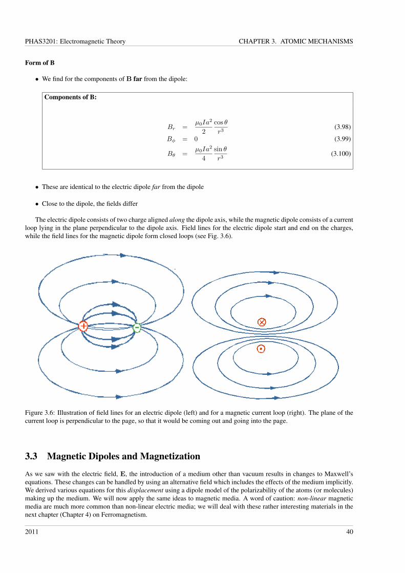
The electric dipole consists of two charge aligned along the dipole axis, while the magnetic dipole consists of a currentloop lying in the plane perpendicular to the dipole axis. Field lines for the electric dipole start and end on the charges,while the field lines for the magnetic dipole form closed loops (see Fig. 3.6).
Figure 3.6: Illustration of field lines for an electric dipole (left) and for a magnetic current loop (right). The plane of thecurrent loop is perpendicular to the page, so that it would be coming out and going into the page.
3.3 Magnetic Dipoles and Magnetization
As we saw with the electric field, E, the introduction of a medium other than vacuum results in changes to Maxwell’sequations. These changes can be handled by using an alternative field which includes the effects of the medium implicitly.We derived various equations for this displacement using a dipole model of the polarizability of the atoms (or molecules)making up the medium. We will now apply the same ideas to magnetic media. A word of caution: non-linear magneticmedia are much more common than non-linear electric media; we will deal with these rather interesting materials in thenext chapter (Chapter 4) on Ferromagnetism.
2011 40
PHAS3201: Electromagnetic Theory CHAPTER 3. ATOMIC MECHANISMS
Magnetization
• We introduced the polarizability of a dielectric material, P ∝ E
• Similarly, we introduce a quantity, proportional to the magnetic induction B
• This is the magnetization, M
• It describes the response of a material to the magnetic induction
• Electrons move in loops around atoms: we can use the magnetic dipole to model the response
Microscopic Origin
• Consider a small piece of a material of volume ∆V
• If mi is the dipole due to the ith atom in ∆V , we define:
M = lim∆V→0
1
∆V
∑i
mi (3.101)
• This is analogous to the polarization (electric dipole moment per unit volume)
• With no field, the directions are random and M = 0
• We will now consider magnetization currents arising from dipoles
Approach
• We will consider a given body made up from adjacent current loops
• We find three simple limits:
1. Uniformly magnetised bulk: No net magnetization current
2. Non-uniformly magnetised bulk: volume magnetization current
3. Uniformly magnetised slab: surface magnetization current
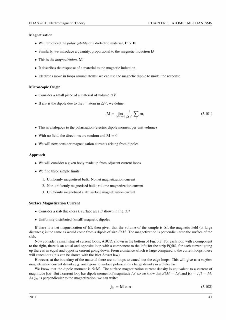
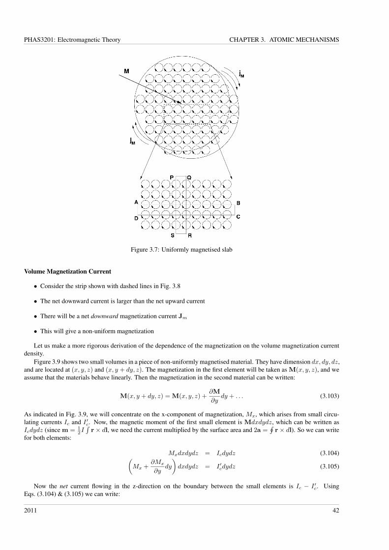
Surface Magnetization Current
• Consider a slab thickness t, surface area S shown in Fig. 3.7
• Uniformly distributed (small) magnetic dipoles
If there is a net magnetization of M, then given that the volume of the sample is St, the magnetic field (at largedistances) is the same as would come from a dipole of size StM . The magnetization is perpendicular to the surface of theslab.
Now consider a small strip of current loops, ABCD, shown in the bottom of Fig. 3.7. For each loop with a componentto the right, there is an equal and opposite loop with a component to the left; for the strip PQRS, for each current goingup there is an equal and opposite current going down. From a distance which is large compared to the current loops, thesewill cancel out (this can be shown with the Biot-Savart law).
However, at the boundary of the material there are no loops to cancel out the edge loops. This will give us a surfacemagnetization current density jM, analogous to surface polarization charge density in a dielectric.
We know that the dipole moment is StM. The surface magnetization current density is equivalent to a current ofmagnitude jMt. But a current loop has dipole moment of magnitude IS, so we know that StM = IS, and jM = I/t = M .As jM is perpendicular to the magnetization, we can write:
jM = M× n (3.102)
2011 41
PHAS3201: Electromagnetic Theory CHAPTER 3. ATOMIC MECHANISMS
Figure 3.7: Uniformly magnetised slab
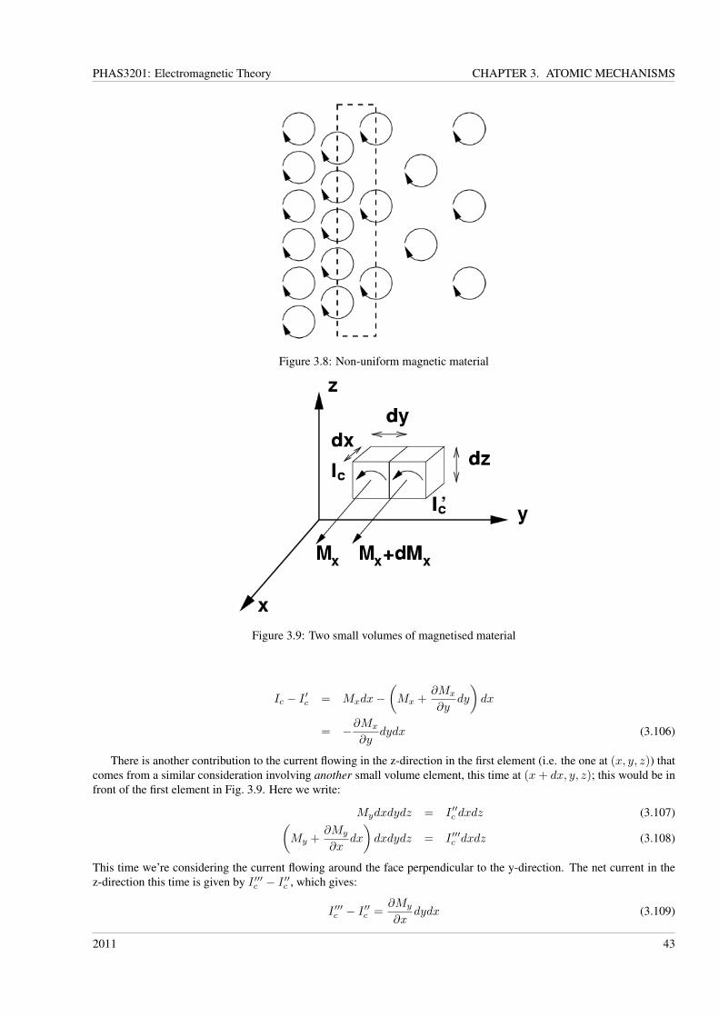
Volume Magnetization Current
• Consider the strip shown with dashed lines in Fig. 3.8
• The net downward current is larger than the net upward current
• There will be a net downward magnetization current Jm
• This will give a non-uniform magnetization
Let us make a more rigorous derivation of the dependence of the magnetization on the volume magnetization currentdensity.
Figure 3.9 shows two small volumes in a piece of non-uniformly magnetised material. They have dimension dx, dy, dz,and are located at (x, y, z) and (x, y + dy, z). The magnetization in the first element will be taken as M(x, y, z), and weassume that the materials behave linearly. Then the magnetization in the second material can be written:
M(x, y + dy, z) = M(x, y, z) +∂M
∂ydy + . . . (3.103)
As indicated in Fig. 3.9, we will concentrate on the x-component of magnetization, Mx, which arises from small circu-lating currents Ic and I ′c. Now, the magnetic moment of the first small element is Mdxdydz, which can be written asIcdydz (since m = 1
2I∫r× dl, we need the current multiplied by the surface area and 2a =
∮r× dl). So we can write
for both elements:
Mxdxdydz = Icdydz (3.104)(Mx +
∂Mx
∂ydy
)dxdydz = I ′cdydz (3.105)
Now the net current flowing in the z-direction on the boundary between the small elements is Ic − I ′c. UsingEqs. (3.104) & (3.105) we can write:
2011 42
PHAS3201: Electromagnetic Theory CHAPTER 3. ATOMIC MECHANISMS
Figure 3.8: Non-uniform magnetic material
Figure 3.9: Two small volumes of magnetised material
Ic − I ′c = Mxdx−(Mx +
∂Mx
∂ydy
)dx
= −∂Mx
∂ydydx (3.106)
There is another contribution to the current flowing in the z-direction in the first element (i.e. the one at (x, y, z)) thatcomes from a similar consideration involving another small volume element, this time at (x+ dx, y, z); this would be infront of the first element in Fig. 3.9. Here we write:
Mydxdydz = I ′′c dxdz (3.107)(My +
∂My
∂xdx
)dxdydz = I ′′′c dxdz (3.108)
This time we’re considering the current flowing around the face perpendicular to the y-direction. The net current in thez-direction this time is given by I ′′′c − I ′′c , which gives:
I ′′′c − I ′′c =∂My
∂xdydx (3.109)
2011 43
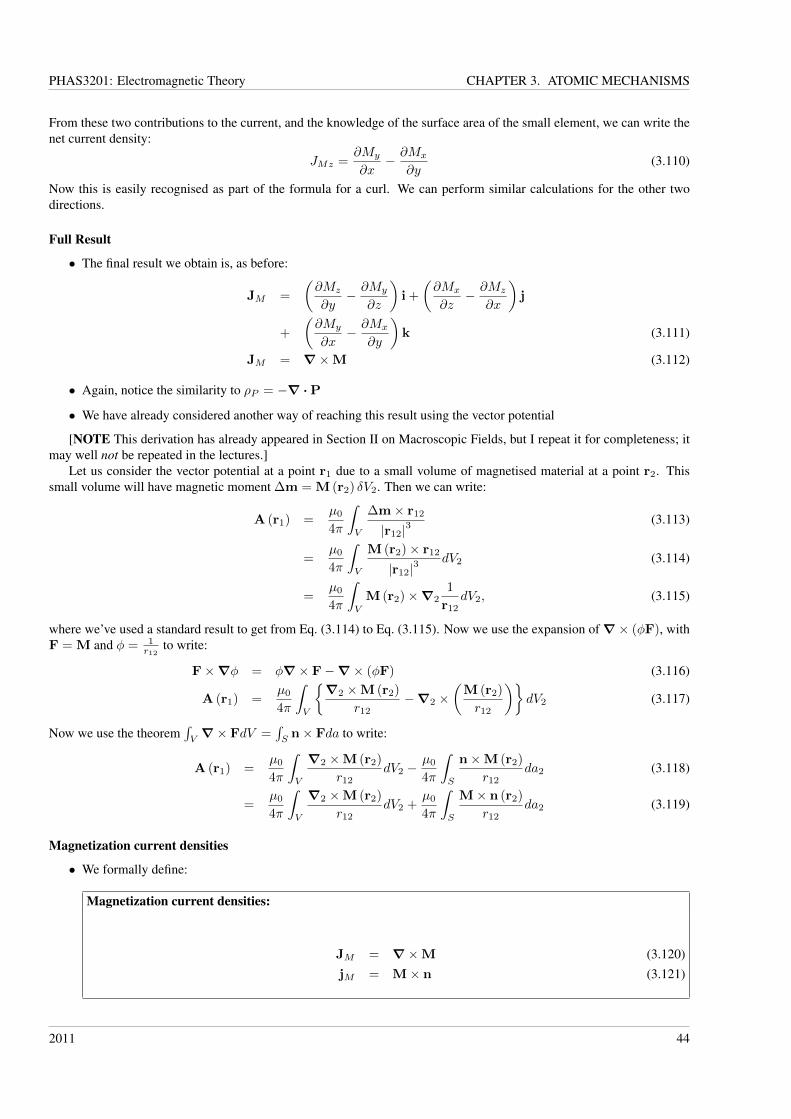
PHAS3201: Electromagnetic Theory CHAPTER 3. ATOMIC MECHANISMS
From these two contributions to the current, and the knowledge of the surface area of the small element, we can write thenet current density:
JMz =∂My
∂x− ∂Mx
∂y(3.110)
Now this is easily recognised as part of the formula for a curl. We can perform similar calculations for the other twodirections.
Full Result
• The final result we obtain is, as before:
JM =
(∂Mz
∂y− ∂My
∂z
)i +
(∂Mx
∂z− ∂Mz
∂x
)j
+
(∂My
∂x− ∂Mx
∂y
)k (3.111)
JM = ∇×M (3.112)
• Again, notice the similarity to ρP = −∇ ·P
• We have already considered another way of reaching this result using the vector potential
[NOTE This derivation has already appeared in Section II on Macroscopic Fields, but I repeat it for completeness; itmay well not be repeated in the lectures.]
Let us consider the vector potential at a point r1 due to a small volume of magnetised material at a point r2. Thissmall volume will have magnetic moment ∆m = M (r2) δV2. Then we can write:
A (r1) =µ0
4π
∫V
∆m× r12
|r12|3(3.113)
=µ0
4π
∫V
M (r2)× r12
|r12|3dV2 (3.114)
=µ0
4π
∫V
M (r2)×∇21
r12dV2, (3.115)
where we’ve used a standard result to get from Eq. (3.114) to Eq. (3.115). Now we use the expansion of∇× (φF), withF = M and φ = 1
r12to write:
F×∇φ = φ∇× F−∇× (φF) (3.116)
A (r1) =µ0
4π
∫V
{∇2 ×M (r2)
r12−∇2 ×
(M (r2)
r12
)}dV2 (3.117)
Now we use the theorem∫V∇× FdV =
∫Sn× Fda to write:
A (r1) =µ0
4π
∫V
∇2 ×M (r2)
r12dV2 −
µ0
4π
∫S
n×M (r2)
r12da2 (3.118)
=µ0
4π
∫V
∇2 ×M (r2)
r12dV2 +
µ0
4π
∫S
M× n (r2)
r12da2 (3.119)
Magnetization current densities
• We formally define:
Magnetization current densities:
JM = ∇×M (3.120)jM = M× n (3.121)
2011 44
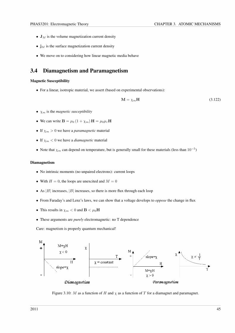
PHAS3201: Electromagnetic Theory CHAPTER 3. ATOMIC MECHANISMS
• JM is the volume magnetization current density
• jM is the surface magnetization current density
• We move on to considering how linear magnetic media behave
3.4 Diamagnetism and Paramagnetism
Magnetic Susceptibility
• For a linear, isotropic material, we assert (based on experimental observations):
M = χmH (3.122)
• χm is the magnetic susceptibility
• We can write B = µ0 (1 + χm)H = µ0µrH
• If χm > 0 we have a paramagnetic material
• If χm < 0 we have a diamagnetic material
• Note that χm can depend on temperature, but is generally small for these materials (less than 10−5)
Diamagnetism
• No intrinsic moments (no unpaired electrons): current loops
• With H = 0, the loops are unexcited and M = 0
• As |H| increases, |B| increases, so there is more flux through each loop
• From Faraday’s and Lenz’s laws, we can show that a voltage develops to oppose the change in flux
• This results in χm < 0 and B < µ0H
• These arguments are purely electromagnetic: no T dependence
Care: magnetism is properly quantum mechanical!
Figure 3.10: M as a function of H and χ as a function of T for a diamagnet and paramagnet.
2011 45
PHAS3201: Electromagnetic Theory CHAPTER 3. ATOMIC MECHANISMS
Paramagnetism
• Some free intrinsic moments (e.g. unpaired electrons)
• With no external field, these are randomly aligned, M = 0 (thermal fluctuation)
• As H increases, they experience a torque aligning them with H
• So χm > 0 and B > µ0H, where m0 is the magnetic moment on each component of the system
• However, this is opposed by random thermal fluctuations
• Thermodynamic analysis gives Curie’s law:
χm =Nm2
0µ0
3kT(3.123)
• There is also often competition between diamagnetic and paramagnetic effects, so χm = Nm20µ0/3kT + χdia
• At low T , paramagnetic effects dominate
2011 46
PHAS3201: Electromagnetic Theory CHAPTER 4. FERROMAGNETISM
Chapter 4
Ferromagnetism
A wonder of such nature I experienced as a child of 4 or 5 years, when my father showed me a compass. Thatthis needle behaved in such a determined way did not at all fit into the nature of events which could find aplace in the unconscious world of concepts (effects connected with direct touch). I can still remember - or atleast believe I can remember - that this experience made a deep and lasting impression upon me. Somethingdeeply hidden had to be behind things.
- A. Einstein
Ferromagnetism represents the earliest discovery of a phenomenon which results from quantum phenomena: lode-stones were used in navigation by the Phoenicians several thousand years ago, while the detailed understanding of ferro-magnetism was not worked out until 1928 (by Heisenberg). We will cover the details at a qualitative level only.
4.1 Atomic-level Picture
We start by considering the effect of the unpaired electron in the 3d shell.
Intrinsic Moments
• There are intrinsic moments at the atomic level
• Unpaired electron spins give the direction of the moments
• There is a strong short range force between neighbouring atoms
• The atoms will align in the lowest energy configuration
In ferromagnetic materials, the configuration which has the lowest potential energy is with the spins aligned parallelto each other. This is not what would be expected from a simple picture of bar magnets, for instance. A full understandingof the phenomenon requires a careful quantum mechanical treatment of the problem, which turns out to arise from anexchange integral and the Pauli exclusion principle. An approximate, classical understanding was first put forward byWeiss who postulated the existence of an unspecified field (now known as the Weiss, or mean, molecular field) such that:
Hm = γM. (4.1)
In other words, there is some field due to the magnetic moments at the atomic level. For a ferromagnetic material, thevalue of M must arise to a large extent from the individual moments, Nm0 (where m0 is the individual moment). Thisrequires a value of γ to be around 1,000; a simple derivation similar to that used for dielectrics and polarization wouldpredict 1
3 . Nevertheless, if this theory is followed through, it predicts a change of magnetization with temperature whichis in approximate agreement with experimental measurements, including a prediction that there is a temperature at whichthe spontaneous magnetization vanishes (the Curie temperature).
2011 47
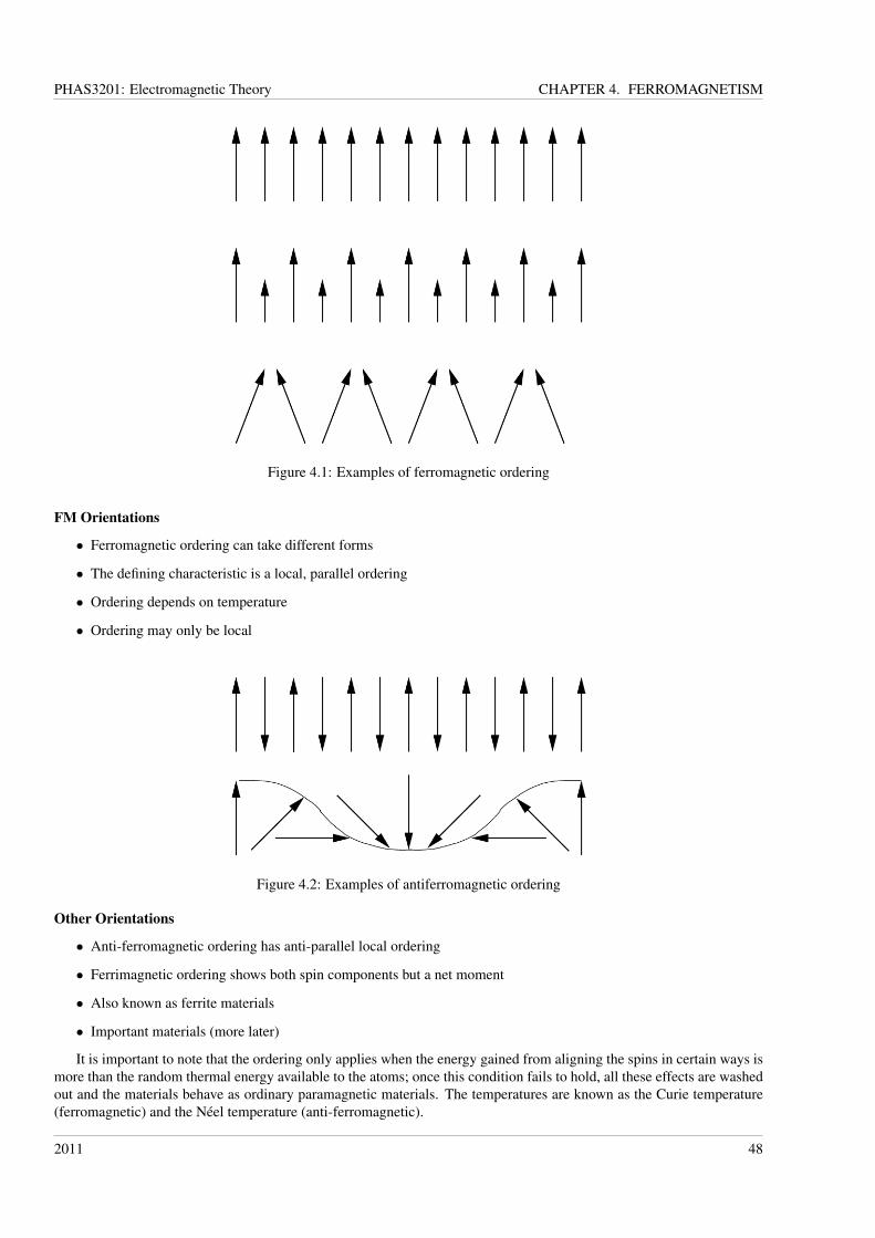
PHAS3201: Electromagnetic Theory CHAPTER 4. FERROMAGNETISM
Figure 4.1: Examples of ferromagnetic ordering
FM Orientations
• Ferromagnetic ordering can take different forms
• The defining characteristic is a local, parallel ordering
• Ordering depends on temperature
• Ordering may only be local
Figure 4.2: Examples of antiferromagnetic ordering
Other Orientations
• Anti-ferromagnetic ordering has anti-parallel local ordering
• Ferrimagnetic ordering shows both spin components but a net moment
• Also known as ferrite materials
• Important materials (more later)
It is important to note that the ordering only applies when the energy gained from aligning the spins in certain ways ismore than the random thermal energy available to the atoms; once this condition fails to hold, all these effects are washedout and the materials behave as ordinary paramagnetic materials. The temperatures are known as the Curie temperature(ferromagnetic) and the Néel temperature (anti-ferromagnetic).
2011 48
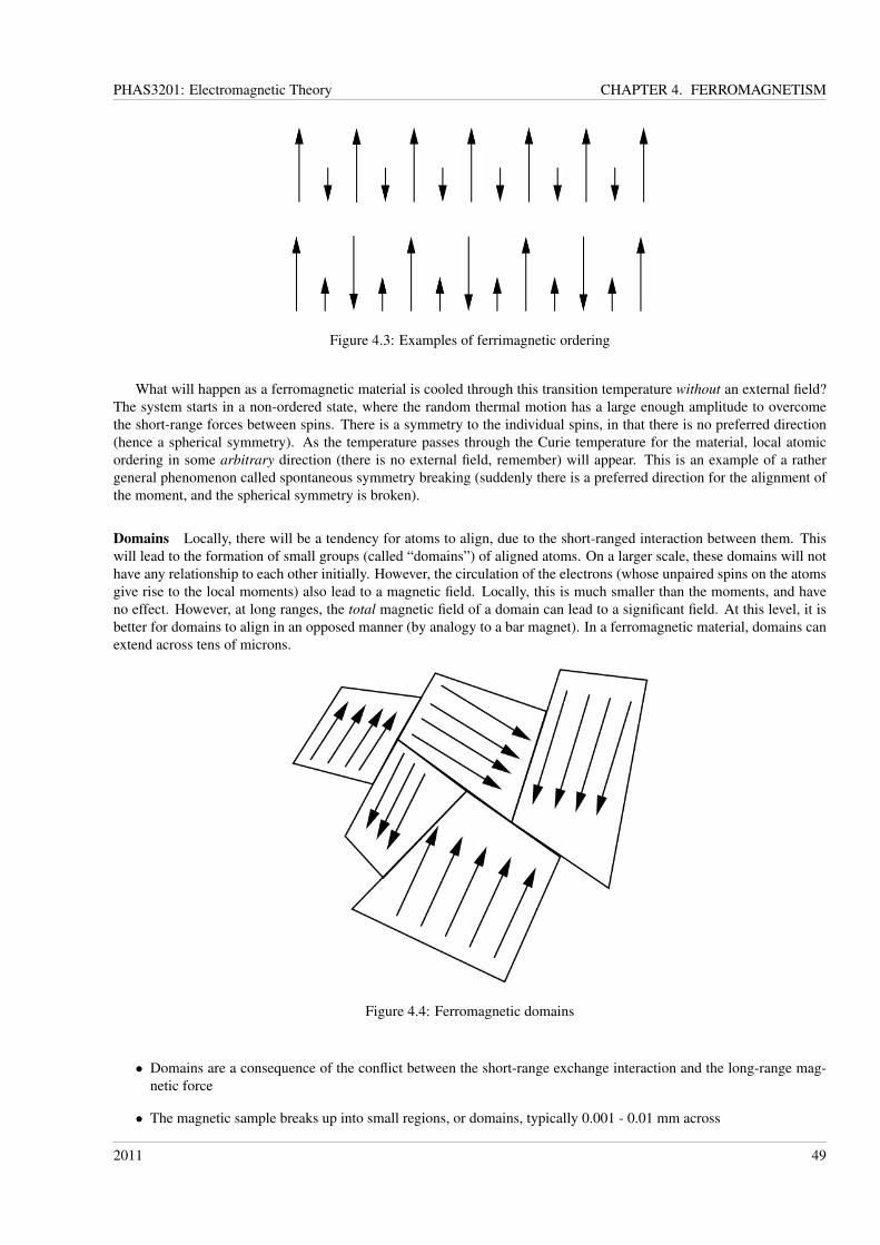
PHAS3201: Electromagnetic Theory CHAPTER 4. FERROMAGNETISM
Figure 4.3: Examples of ferrimagnetic ordering
What will happen as a ferromagnetic material is cooled through this transition temperature without an external field?The system starts in a non-ordered state, where the random thermal motion has a large enough amplitude to overcomethe short-range forces between spins. There is a symmetry to the individual spins, in that there is no preferred direction(hence a spherical symmetry). As the temperature passes through the Curie temperature for the material, local atomicordering in some arbitrary direction (there is no external field, remember) will appear. This is an example of a rathergeneral phenomenon called spontaneous symmetry breaking (suddenly there is a preferred direction for the alignment ofthe moment, and the spherical symmetry is broken).
Domains Locally, there will be a tendency for atoms to align, due to the short-ranged interaction between them. Thiswill lead to the formation of small groups (called “domains”) of aligned atoms. On a larger scale, these domains will nothave any relationship to each other initially. However, the circulation of the electrons (whose unpaired spins on the atomsgive rise to the local moments) also lead to a magnetic field. Locally, this is much smaller than the moments, and haveno effect. However, at long ranges, the total magnetic field of a domain can lead to a significant field. At this level, it isbetter for domains to align in an opposed manner (by analogy to a bar magnet). In a ferromagnetic material, domains canextend across tens of microns.
Figure 4.4: Ferromagnetic domains
• Domains are a consequence of the conflict between the short-range exchange interaction and the long-range mag-netic force
• The magnetic sample breaks up into small regions, or domains, typically 0.001 - 0.01 mm across
2011 49
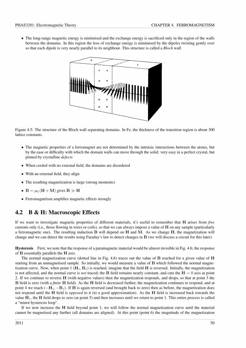
PHAS3201: Electromagnetic Theory CHAPTER 4. FERROMAGNETISM
• The long-range magnetic energy is minimised and the exchange energy is sacrificed only in the region of the wallsbetween the domains. In this region the loss of exchange energy is minimised by the dipoles twisting gently overso that each dipole is very nearly parallel to its neighbour. This structure is called a Bloch wall
Figure 4.5: The structure of the Bloch wall separating domains. In Fe, the thickness of the transition region is about 300lattice constants.
• The magnetic properties of a ferromagnet are not determined by the intrinsic interactions between the atoms, butby the ease or difficulty with which the domain walls can move through the solid: very easy in a perfect crystal, butpinned by crystalline defects
• When cooled with no external field, the domains are disordered
• With an external field, they align
• The resulting magnetization is large (strong moments)
• B = µ0 (H + M) gives B� H
• Ferromagnetism amplifies magnetic effects strongly
4.2 B & H: Macroscopic EffectsIf we want to investigate magnetic properties of different materials, it’s useful to remember that H arises from freecurrents only (i.e., those flowing in wires or coils), so that we can always impose a value of H on any sample (particularlya ferromagnetic one). The resulting induction B will depend on H and M. As we change H, the magnetization willchange and we can detect the results using Faraday’s law to detect changes in B (we will discuss a circuit for this later).
Hysteresis First, we note that the response of a paramagnetic material would be almost invisible in Fig. 4.6; the responseof B essentially parallels the H axis.
The normal magnetization curve (dotted line in Fig. 4.6) traces out the value of B reached for a given value of Hstarting from an unmagnetised sample. So initially, we would measure a value of B which followed the normal magne-tization curve. Now, when point 1 (H1,B1) is reached, imagine that the field H is reversed. Initially, the magnetizationis not affected, and the normal curve is not traced; the B field remains nearly constant, and cuts the H = 0 axis at point2. If we continue to reverse H (with negative values) then the magnetization responds, and drops, so that at point 3 theB field is zero (with a finite H field). As the H field is decreased further, the magnetization continues to respond, and atpoint 4 we reach (−H1,−B1). If H is again reversed (and brought back to zero) then as before, the magnetization doesnot respond until the H field is opposed to it (to a good approximation). As the H field is increased back towards thevalue H1, the B field drops to zero (at point 5) and then increases until we return to point 1. This entire process is calleda “minor hysteresis loop”.
If we now increase the H field beyond point 1, we will follow the normal magnetization curve until the materialcannot be magnetised any further (all domains are aligned). At this point (point 6) the magnitude of the magnetization
2011 50
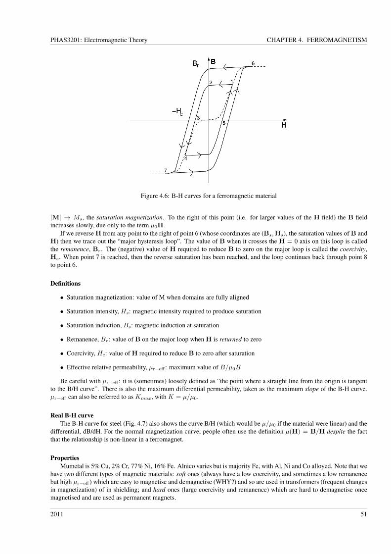
PHAS3201: Electromagnetic Theory CHAPTER 4. FERROMAGNETISM
Figure 4.6: B-H curves for a ferromagnetic material
|M| → Ms, the saturation magnetization. To the right of this point (i.e. for larger values of the H field) the B fieldincreases slowly, due only to the term µ0H.
If we reverse H from any point to the right of point 6 (whose coordinates are (Bs,Hs), the saturation values of B andH) then we trace out the “major hysteresis loop”. The value of B when it crosses the H = 0 axis on this loop is calledthe remanence, Br. The (negative) value of H required to reduce B to zero on the major loop is called the coercivity,Hc. When point 7 is reached, then the reverse saturation has been reached, and the loop continues back through point 8to point 6.
Definitions
• Saturation magnetization: value of M when domains are fully aligned
• Saturation intensity, Hs: magnetic intensity required to produce saturation
• Saturation induction, Bs: magnetic induction at saturation
• Remanence, Br: value of B on the major loop when H is returned to zero
• Coercivity, Hc: value of H required to reduce B to zero after saturation
• Effective relative permeability, µr−eff : maximum value of B/µ0H
Be careful with µr−eff : it is (sometimes) loosely defined as “the point where a straight line from the origin is tangentto the B/H curve”. There is also the maximum differential permeability, taken as the maximum slope of the B-H curve.µr−eff can also be referred to as Kmax, with K = µ/µ0.
Real B-H curveThe B-H curve for steel (Fig. 4.7) also shows the curve B/H (which would be µ/µ0 if the material were linear) and the
differential, dB/dH. For the normal magnetization curve, people often use the definition µ(H) = B/H despite the factthat the relationship is non-linear in a ferromagnet.
PropertiesMumetal is 5% Cu, 2% Cr, 77% Ni, 16% Fe. Alnico varies but is majority Fe, with Al, Ni and Co alloyed. Note that we
have two different types of magnetic materials: soft ones (always have a low coercivity, and sometimes a low remanencebut high µr−eff ) which are easy to magnetise and demagnetise (WHY?) and so are used in transformers (frequent changesin magnetization) of in shielding; and hard ones (large coercivity and remanence) which are hard to demagnetise oncemagnetised and are used as permanent magnets.
2011 51
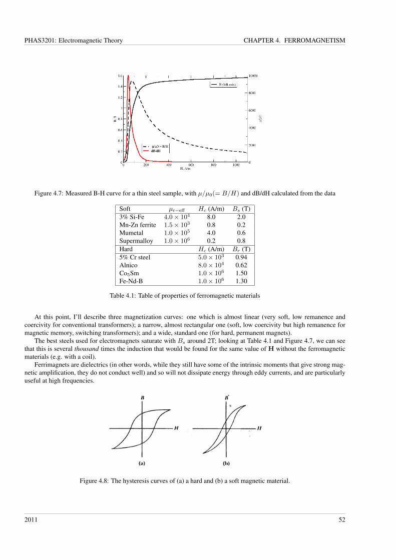
PHAS3201: Electromagnetic Theory CHAPTER 4. FERROMAGNETISM
Figure 4.7: Measured B-H curve for a thin steel sample, with µ/µ0(= B/H) and dB/dH calculated from the data
Soft µr−eff Hc (A/m) Bs (T)3% Si-Fe 4.0× 10⁴ 8.0 2.0Mn-Zn ferrite 1.5× 10³ 0.8 0.2Mumetal 1.0× 10⁵ 4.0 0.6Supermalloy 1.0× 10⁶ 0.2 0.8Hard Hc (A/m) Br (T)5% Cr steel 5.0× 10³ 0.94Alnico 8.0× 10⁴ 0.62Co5Sm 1.0× 10⁶ 1.50Fe-Nd-B 1.0× 10⁶ 1.30
Table 4.1: Table of properties of ferromagnetic materials
At this point, I’ll describe three magnetization curves: one which is almost linear (very soft, low remanence andcoercivity for conventional transformers); a narrow, almost rectangular one (soft, low coercivity but high remanence formagnetic memory, switching transformers); and a wide, standard one (for hard, permanent magnets).
The best steels used for electromagnets saturate with Bs around 2T; looking at Table 4.1 and Figure 4.7, we can seethat this is several thousand times the induction that would be found for the same value of H without the ferromagneticmaterials (e.g. with a coil).
Ferrimagnets are dielectrics (in other words, while they still have some of the intrinsic moments that give strong mag-netic amplification, they do not conduct well) and so will not dissipate energy through eddy currents, and are particularlyuseful at high frequencies.
Figure 4.8: The hysteresis curves of (a) a hard and (b) a soft magnetic material.
2011 52
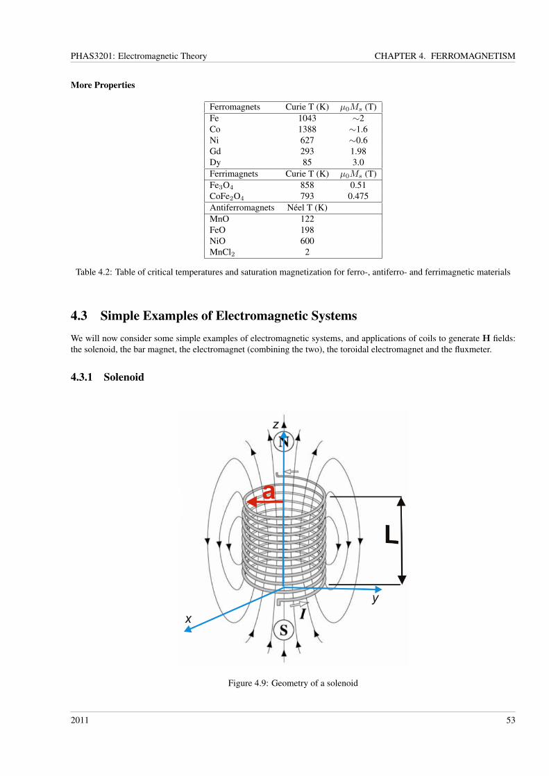
PHAS3201: Electromagnetic Theory CHAPTER 4. FERROMAGNETISM
More Properties
Ferromagnets Curie T (K) µ0Ms (T)Fe 1043 ∼2Co 1388 ∼1.6Ni 627 ∼0.6Gd 293 1.98Dy 85 3.0Ferrimagnets Curie T (K) µ0Ms (T)Fe3O4 858 0.51CoFe2O4 793 0.475Antiferromagnets Néel T (K)MnO 122FeO 198NiO 600MnCl2 2
Table 4.2: Table of critical temperatures and saturation magnetization for ferro-, antiferro- and ferrimagnetic materials
4.3 Simple Examples of Electromagnetic SystemsWe will now consider some simple examples of electromagnetic systems, and applications of coils to generate H fields:the solenoid, the bar magnet, the electromagnet (combining the two), the toroidal electromagnet and the fluxmeter.
4.3.1 Solenoid
Figure 4.9: Geometry of a solenoid
2011 53
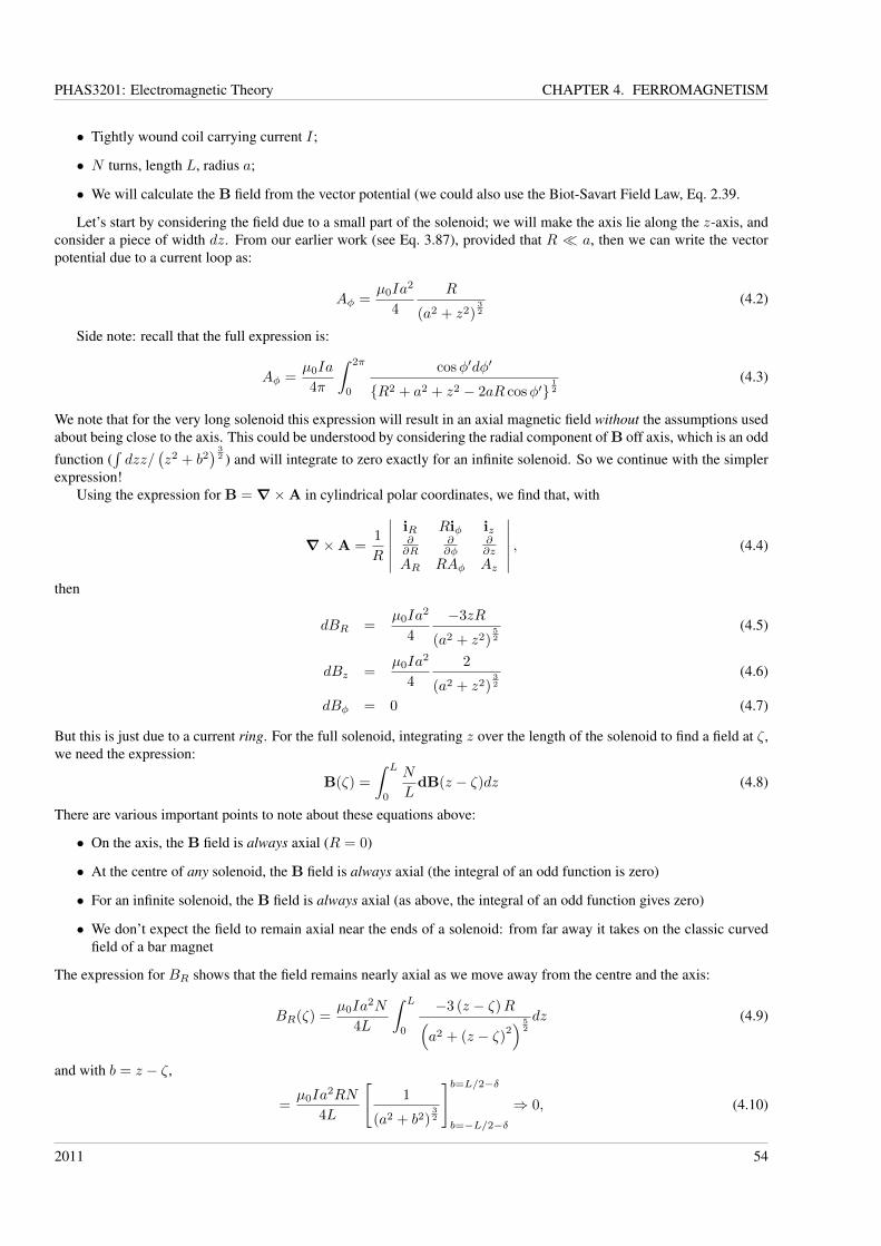
PHAS3201: Electromagnetic Theory CHAPTER 4. FERROMAGNETISM
• Tightly wound coil carrying current I;
• N turns, length L, radius a;
• We will calculate the B field from the vector potential (we could also use the Biot-Savart Field Law, Eq. 2.39.
Let’s start by considering the field due to a small part of the solenoid; we will make the axis lie along the z-axis, andconsider a piece of width dz. From our earlier work (see Eq. 3.87), provided that R � a, then we can write the vectorpotential due to a current loop as:
Aφ =µ0Ia
2
4
R
(a2 + z2)32
(4.2)
Side note: recall that the full expression is:
Aφ =µ0Ia
4π
∫ 2π
0
cosφ′dφ′
{R2 + a2 + z2 − 2aR cosφ′}12
(4.3)
We note that for the very long solenoid this expression will result in an axial magnetic field without the assumptions usedabout being close to the axis. This could be understood by considering the radial component of B off axis, which is an odd
function (∫dzz/
(z2 + b2
) 32 ) and will integrate to zero exactly for an infinite solenoid. So we continue with the simpler
expression!Using the expression for B =∇×A in cylindrical polar coordinates, we find that, with
∇×A =1
R
∣∣∣∣∣∣iR Riφ iz∂∂R
∂∂φ
∂∂z
AR RAφ Az
∣∣∣∣∣∣ , (4.4)
then
dBR =µ0Ia
2
4
−3zR
(a2 + z2)52
(4.5)
dBz =µ0Ia
2
4
2
(a2 + z2)32
(4.6)
dBφ = 0 (4.7)
But this is just due to a current ring. For the full solenoid, integrating z over the length of the solenoid to find a field at ζ,we need the expression:
B(ζ) =
∫ L
0
N
LdB(z − ζ)dz (4.8)
There are various important points to note about these equations above:
• On the axis, the B field is always axial (R = 0)
• At the centre of any solenoid, the B field is always axial (the integral of an odd function is zero)
• For an infinite solenoid, the B field is always axial (as above, the integral of an odd function gives zero)
• We don’t expect the field to remain axial near the ends of a solenoid: from far away it takes on the classic curvedfield of a bar magnet
The expression for BR shows that the field remains nearly axial as we move away from the centre and the axis:
BR(ζ) =µ0Ia
2N
4L
∫ L
0
−3 (z − ζ)R(a2 + (z − ζ)
2) 5
2
dz (4.9)
and with b = z − ζ,
=µ0Ia
2RN
4L
[1
(a2 + b2)32
]b=L/2−δb=−L/2−δ
⇒ 0, (4.10)
2011 54
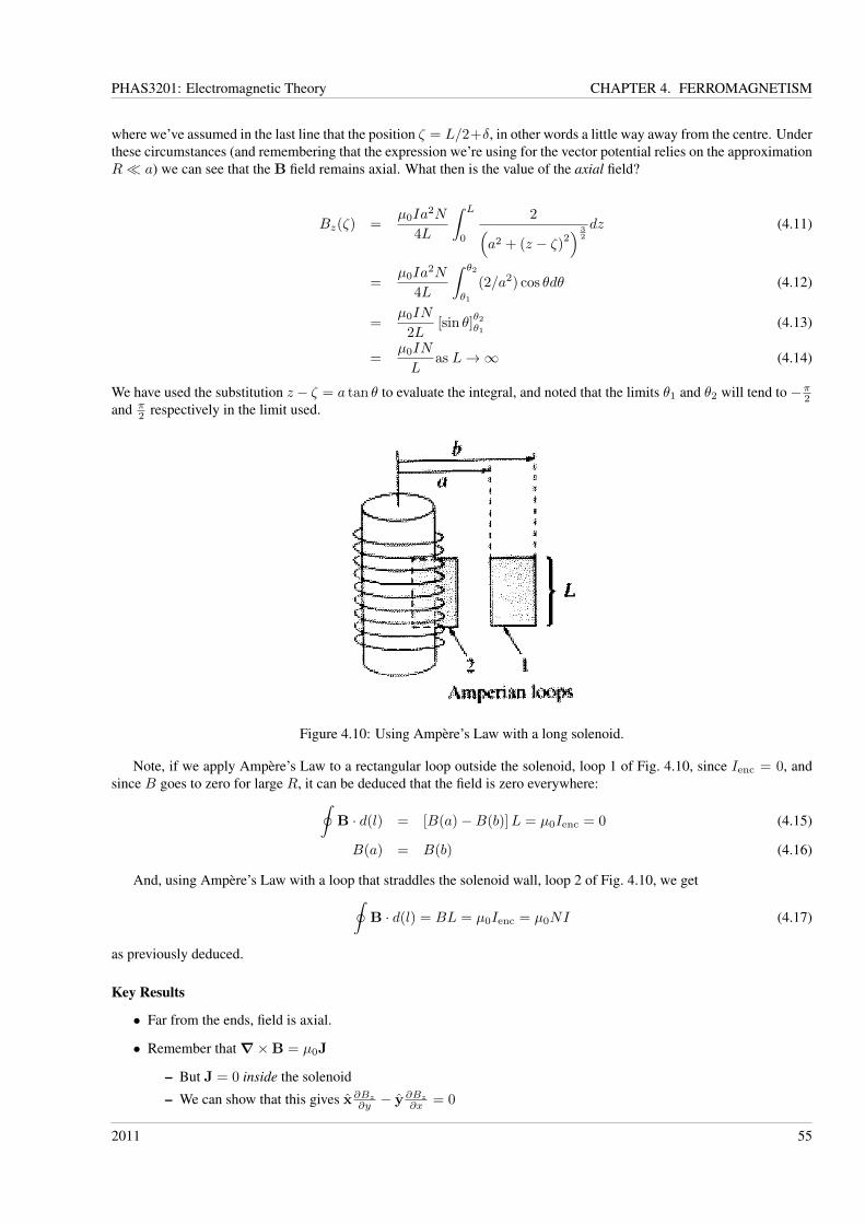
PHAS3201: Electromagnetic Theory CHAPTER 4. FERROMAGNETISM
where we’ve assumed in the last line that the position ζ = L/2+δ, in other words a little way away from the centre. Underthese circumstances (and remembering that the expression we’re using for the vector potential relies on the approximationR� a) we can see that the B field remains axial. What then is the value of the axial field?
Bz(ζ) =µ0Ia
2N
4L
∫ L
0
2(a2 + (z − ζ)
2) 3
2
dz (4.11)
=µ0Ia
2N
4L
∫ θ2
θ1
(2/a2) cos θdθ (4.12)
=µ0IN
2L[sin θ]
θ2θ1
(4.13)
=µ0IN
Las L→∞ (4.14)
We have used the substitution z − ζ = a tan θ to evaluate the integral, and noted that the limits θ1 and θ2 will tend to −π2and π
2 respectively in the limit used.
Figure 4.10: Using Ampère’s Law with a long solenoid.
Note, if we apply Ampère’s Law to a rectangular loop outside the solenoid, loop 1 of Fig. 4.10, since Ienc = 0, andsince B goes to zero for large R, it can be deduced that the field is zero everywhere:∮
B · d(l) = [B(a)−B(b)]L = µ0Ienc = 0 (4.15)
B(a) = B(b) (4.16)
And, using Ampère’s Law with a loop that straddles the solenoid wall, loop 2 of Fig. 4.10, we get∮B · d(l) = BL = µ0Ienc = µ0NI (4.17)
as previously deduced.
Key Results
• Far from the ends, field is axial.
• Remember that∇×B = µ0J
– But J = 0 inside the solenoid
– We can show that this gives x∂Bz∂y − y ∂Bz∂x = 0
2011 55
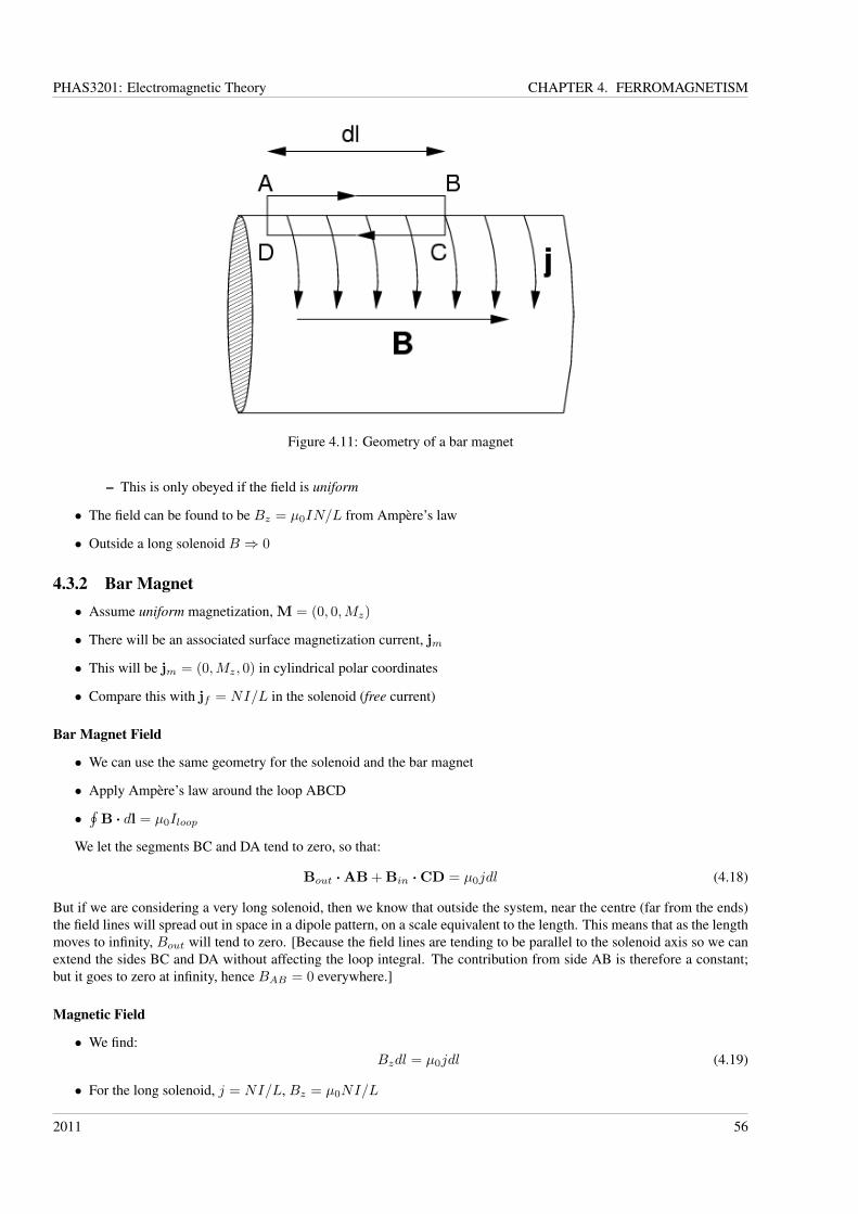
PHAS3201: Electromagnetic Theory CHAPTER 4. FERROMAGNETISM
Figure 4.11: Geometry of a bar magnet
– This is only obeyed if the field is uniform
• The field can be found to be Bz = µ0IN/L from Ampère’s law
• Outside a long solenoid B ⇒ 0
4.3.2 Bar Magnet• Assume uniform magnetization, M = (0, 0,Mz)
• There will be an associated surface magnetization current, jm
• This will be jm = (0,Mz, 0) in cylindrical polar coordinates
• Compare this with jf = NI/L in the solenoid (free current)
Bar Magnet Field
• We can use the same geometry for the solenoid and the bar magnet
• Apply Ampère’s law around the loop ABCD
•∮B · dl = µ0Iloop
We let the segments BC and DA tend to zero, so that:
Bout ·AB + Bin ·CD = µ0jdl (4.18)
But if we are considering a very long solenoid, then we know that outside the system, near the centre (far from the ends)the field lines will spread out in space in a dipole pattern, on a scale equivalent to the length. This means that as the lengthmoves to infinity, Bout will tend to zero. [Because the field lines are tending to be parallel to the solenoid axis so we canextend the sides BC and DA without affecting the loop integral. The contribution from side AB is therefore a constant;but it goes to zero at infinity, hence BAB = 0 everywhere.]
Magnetic Field
• We find:Bzdl = µ0jdl (4.19)
• For the long solenoid, j = NI/L, Bz = µ0NI/L
2011 56
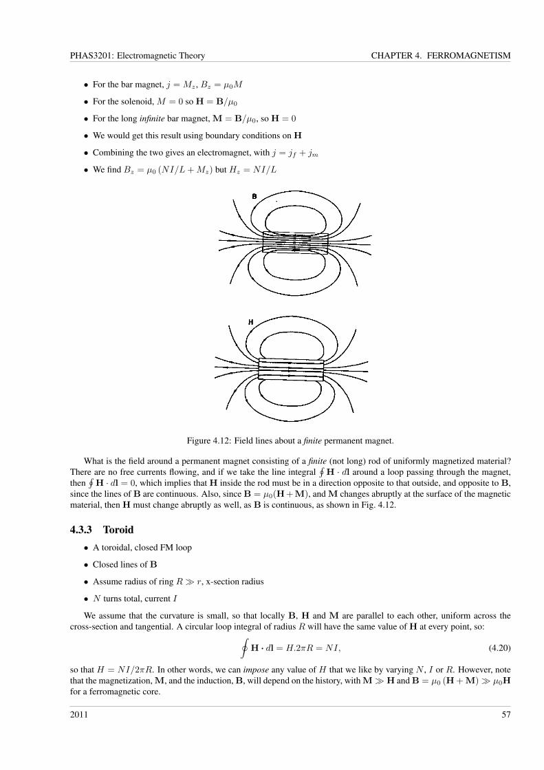
PHAS3201: Electromagnetic Theory CHAPTER 4. FERROMAGNETISM
• For the bar magnet, j = Mz , Bz = µ0M
• For the solenoid, M = 0 so H = B/µ0
• For the long infinite bar magnet, M = B/µ0, so H = 0
• We would get this result using boundary conditions on H
• Combining the two gives an electromagnet, with j = jf + jm
• We find Bz = µ0 (NI/L+Mz) but Hz = NI/L
Figure 4.12: Field lines about a finite permanent magnet.
What is the field around a permanent magnet consisting of a finite (not long) rod of uniformly magnetized material?There are no free currents flowing, and if we take the line integral
∮H · dl around a loop passing through the magnet,
then∮H · dl = 0, which implies that H inside the rod must be in a direction opposite to that outside, and opposite to B,
since the lines of B are continuous. Also, since B = µ0(H+M), and M changes abruptly at the surface of the magneticmaterial, then H must change abruptly as well, as B is continuous, as shown in Fig. 4.12.
4.3.3 Toroid• A toroidal, closed FM loop
• Closed lines of B
• Assume radius of ring R� r, x-section radius
• N turns total, current I
We assume that the curvature is small, so that locally B, H and M are parallel to each other, uniform across thecross-section and tangential. A circular loop integral of radius R will have the same value of H at every point, so:∮
H · dl = H.2πR = NI, (4.20)
so that H = NI/2πR. In other words, we can impose any value of H that we like by varying N , I or R. However, notethat the magnetization, M, and the induction, B, will depend on the history, with M� H and B = µ0 (H + M)� µ0Hfor a ferromagnetic core.
2011 57
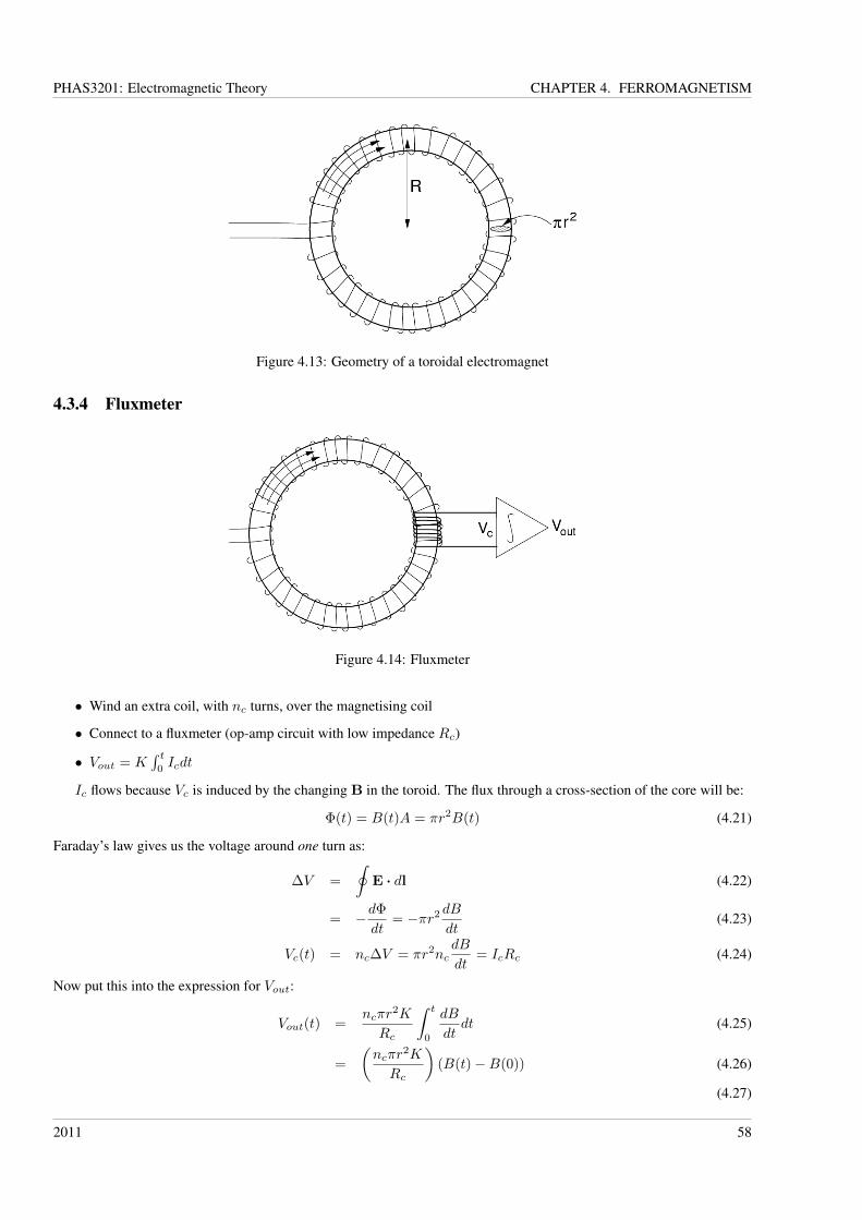
PHAS3201: Electromagnetic Theory CHAPTER 4. FERROMAGNETISM
Figure 4.13: Geometry of a toroidal electromagnet
4.3.4 Fluxmeter
Figure 4.14: Fluxmeter
• Wind an extra coil, with nc turns, over the magnetising coil
• Connect to a fluxmeter (op-amp circuit with low impedance Rc)
• Vout = K∫ t
0Icdt
Ic flows because Vc is induced by the changing B in the toroid. The flux through a cross-section of the core will be:
Φ(t) = B(t)A = πr2B(t) (4.21)
Faraday’s law gives us the voltage around one turn as:
∆V =
∮E · dl (4.22)
= −dΦ
dt= −πr2 dB
dt(4.23)
Vc(t) = nc∆V = πr2ncdB
dt= IcRc (4.24)
Now put this into the expression for Vout:
Vout(t) =ncπr
2K
Rc
∫ t
0
dB
dtdt (4.25)
=
(ncπr
2K
Rc
)(B(t)−B(0)) (4.26)
(4.27)
2011 58
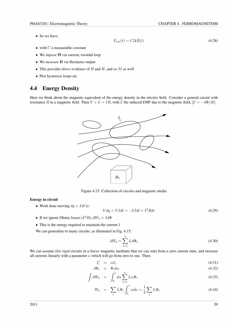
PHAS3201: Electromagnetic Theory CHAPTER 4. FERROMAGNETISM
• So we have:Vout(t) = C∆B(t) (4.28)
• with C a measurable constant
• We impose H via current, toroidal loop
• We measure B via fluxmeter output
• This provides direct evidence of B and H , and so M as well
• Plot hysteresis loops etc
4.4 Energy DensityHere we think about the magnetic equivalent of the energy density in the electric field. Consider a general circuit withresistance R in a magnetic field. Then V + E = IR, with E the induced EMF due to the magnetic field, [E = −dΦ/dt].
Figure 4.15: Collection of circuits and magnetic media
Energy in circuit
• Work done moving dq = Idt is:V dq = V Idt = −EIdt+ I2Rdt (4.29)
• If we ignore Ohmic losses (I2R), dWb = IdΦ
• This is the energy required to maintain the current I
We can generalise to many circuits, as illustrated in Fig. 4.15:
dWb =
n∑i=1
IidΦi (4.30)
We can assume (for rigid circuits in a linear magnetic medium) that we can start from a zero current state, and increaseall currents linearly with a parameter α which will go from zero to one. Then:
I ′i = αIi (4.31)dΦi = Φidα (4.32)∫dWb =
∫ 1
0
dα
n∑i=1
IiαΦi (4.33)
Wb =∑i
IiΦi
∫ 1
0
αdα =1
2
∑i
IiΦi (4.34)
2011 59
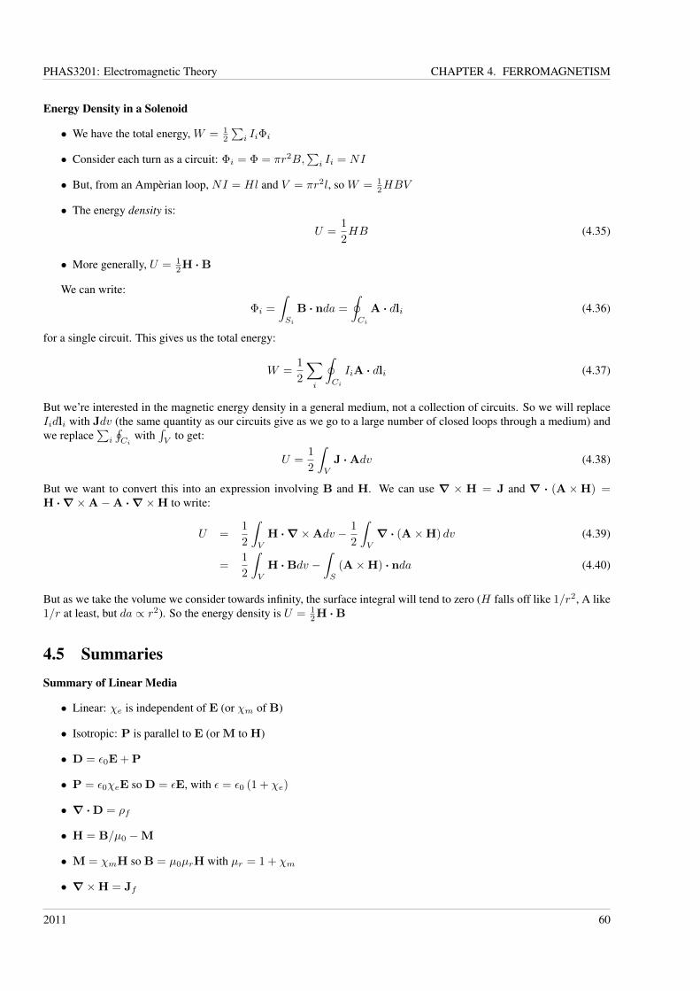
PHAS3201: Electromagnetic Theory CHAPTER 4. FERROMAGNETISM
Energy Density in a Solenoid
• We have the total energy, W = 12
∑i IiΦi
• Consider each turn as a circuit: Φi = Φ = πr2B,∑i Ii = NI
• But, from an Ampèrian loop, NI = Hl and V = πr2l, so W = 12HBV
• The energy density is:
U =1
2HB (4.35)
• More generally, U = 12H ·B
We can write:
Φi =
∫Si
B · nda =
∮Ci
A · dli (4.36)
for a single circuit. This gives us the total energy:
W =1
2
∑i
∮Ci
IiA · dli (4.37)
But we’re interested in the magnetic energy density in a general medium, not a collection of circuits. So we will replaceIidli with Jdv (the same quantity as our circuits give as we go to a large number of closed loops through a medium) andwe replace
∑i
∮Ci
with∫V
to get:
U =1
2
∫V
J ·Adv (4.38)
But we want to convert this into an expression involving B and H. We can use ∇ × H = J and ∇ · (A×H) =H · ∇×A−A · ∇×H to write:
U =1
2
∫V
H · ∇×Adv − 1
2
∫V
∇ · (A×H) dv (4.39)
=1
2
∫V
H ·Bdv −∫S
(A×H) · nda (4.40)
But as we take the volume we consider towards infinity, the surface integral will tend to zero (H falls off like 1/r2, A like1/r at least, but da ∝ r2). So the energy density is U = 1
2H ·B
4.5 SummariesSummary of Linear Media
• Linear: χe is independent of E (or χm of B)
• Isotropic: P is parallel to E (or M to H)
• D = ε0E + P
• P = ε0χeE so D = εE, with ε = ε0 (1 + χe)
• ∇ ·D = ρf
• H = B/µ0 −M
• M = χmH so B = µ0µrH with µr = 1 + χm
• ∇×H = Jf
2011 60
PHAS3201: Electromagnetic Theory CHAPTER 4. FERROMAGNETISM
Summary of Non-Linear Media
• Unpaired electrons give intrinsic moment
• There is a short-range force which aligns these spins
• If parallel, ferromagnetic ordering
• If anti-parallel, anti-ferromagnetic ordering
• Local domains of aligned atoms form (up to microns across)
• Long-range forces arrange these opposed to each other
• Highly non-linear B vs. H curves: hysteresis
• Energy density, U = 12B ·H
2011 61
PHAS3201: Electromagnetic Theory CHAPTER 4. FERROMAGNETISM
2011 62
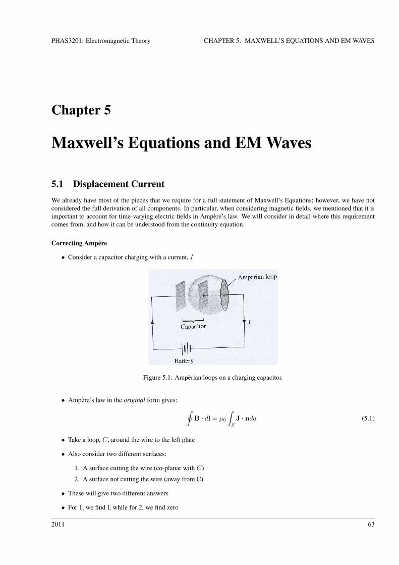
PHAS3201: Electromagnetic Theory CHAPTER 5. MAXWELL’S EQUATIONS AND EM WAVES
Chapter 5
Maxwell’s Equations and EM Waves
5.1 Displacement CurrentWe already have most of the pieces that we require for a full statement of Maxwell’s Equations; however, we have notconsidered the full derivation of all components. In particular, when considering magnetic fields, we mentioned that it isimportant to account for time-varying electric fields in Ampère’s law. We will consider in detail where this requirementcomes from, and how it can be understood from the continuity equation.
Correcting Ampère
• Consider a capacitor charging with a current, I
Figure 5.1: Ampèrian loops on a charging capacitor.
• Ampère’s law in the original form gives: ∮B · dl = µ0
∫S
J · nda (5.1)
• Take a loop, C, around the wire to the left plate
• Also consider two different surfaces:
1. A surface cutting the wire (co-planar with C)
2. A surface not cutting the wire (away from C)
• These will give two different answers
• For 1, we find I, while for 2, we find zero
2011 63
PHAS3201: Electromagnetic Theory CHAPTER 5. MAXWELL’S EQUATIONS AND EM WAVES
Where does the problem come from? Let us consider a closed surface integral over the current density by joiningtogether the two surfaces mentioned above. In this case, we note that there is a net inflow of charge (which sits on theplate of the capacitor inside the surface). We turn to the continuity equation to correct this problem, but where does itcome from? As with many parts of electromagnetism, it is an empirically derived observation. We can define the currentdensity in a general volume of space as:
J =∑i
Niqivi, (5.2)
where we sum over the different types of charge carrier, and Ni gives the number of charge carriers of type i per unitvolume. The current passing through an element of area, da, is dI = J · nda. Then the current through an arbitrarysurface S can be written:
I = −∮S
J · nda = −∫∇ · Jdv, (5.3)
where we have used the divergence theorem, and have a minus sign because charge is flowing into the volume.Here we have defined current in terms of the rate of flow of charge. But we could also define something with the
dimensions of current as the rate of accumulation of charge in some region. Now the current is defined as I = dQdt which
we can write as:
I =dQ
dt=
d
dt
∫V
ρdv
=
∫V
∂ρ
∂tdv, (5.4)
since the volume is fixed in time. The law of conservation of charge says that these two currents are in fact the same thing,so equating them we find: ∫
V
∂ρ
∂tdv = −
∫∇ · Jdv
⇒∫v
(∂ρ
∂t+∇ · J
)dv = 0. (5.5)
There is only one way that this can be fulfilled for an arbitrary volume, V . We require:
∇ · J +∂ρ
∂t= 0. (5.6)
This is the continuity equation (which assumes that charge is conserved).Let us return to Ampère’s law, and remind ourselves of the differential form:
∇×H = Jf . (5.7)
Now if we take the divergence, we find
∇ · (∇×H) (= 0) =∇ · Jf , (5.8)
where we have used the identity that the divergence of a curl is zero. (Note that we’ll use this idea again in little while.)So we have to change eq. (5.7) to account for the change of charge density and its associated fields with time. Since∇ ·D = ρf , we can rewrite the continuity equation as follows:
∇ · Jf +∂∇ ·D∂t
= 0 (5.9)
∇ ·(Jf +
∂D
∂t
)= 0 (5.10)
(5.11)
It was Maxwell’s insight to suggest that if we replace the term J in Ampère’s law with Jf + ∂D∂t then taking the
divergence of Ampère’s Law would make sense. This gives use the Ampère-Maxwell equation:
2011 64
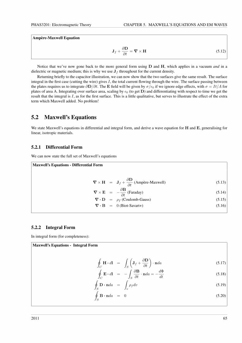
PHAS3201: Electromagnetic Theory CHAPTER 5. MAXWELL’S EQUATIONS AND EM WAVES
Ampère-Maxwell Equation
Jf +∂D
∂t=∇×H (5.12)
Notice that we’ve now gone back to the more general form using D and H, which applies in a vacuum and in adielectric or magnetic medium; this is why we use Jf throughout for the current density.
Returning briefly to the capacitor illustration, we can now show that the two surfaces give the same result. The surfaceintegral in the first case (cutting the wire) gives I , the total current flowing through the wire. The surface passing betweenthe plates requires us to integrate ∂D/∂t. The E field will be given by σ/ε0 if we ignore edge effects, with σ = It/A forplates of area A. Integrating over surface area, scaling by ε0 (to get D) and differentiating with respect to time we get theresult that the integral is I , as for the first surface. This is a little qualitative, but serves to illustrate the effect of the extraterm which Maxwell added. No problem!
5.2 Maxwell’s Equations
We state Maxwell’s equations in differential and integral form, and derive a wave equation for H and E, generalising forlinear, isotropic materials.
5.2.1 Differential Form
We can now state the full set of Maxwell’s equations
Maxwell’s Equations - Differential Form
∇×H = Jf +∂D
∂t(Ampère-Maxwell) (5.13)
∇×E = −∂B∂t
(Faraday) (5.14)
∇ ·D = ρf (Coulomb-Gauss) (5.15)∇ ·B = 0 (Biot-Savart+) (5.16)
5.2.2 Integral Form
In integral form (for completeness):
Maxwell’s Equations - Integral Form
∮C
H · dl =
∫S
(Jf +
∂D
∂t
)· nda (5.17)∮
C
E · dl = −∫S
∂B
∂t· nda = −dΦ
dt(5.18)∮
S
D · nda =
∫v
ρfdv (5.19)∮S
B · nda = 0 (5.20)
2011 65
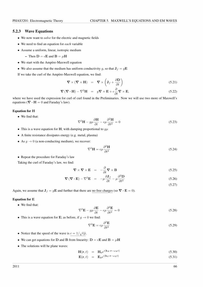
PHAS3201: Electromagnetic Theory CHAPTER 5. MAXWELL’S EQUATIONS AND EM WAVES
5.2.3 Wave Equations• We now want to solve for the electric and magnetic fields
• We need to find an equation for each variable
• Assume a uniform, linear, isotropic medium
– Then D = εE and B = µH
• We start with the Ampère-Maxwell equation
• We also assume that the medium has uniform conductivity g, so that Jf = gE
If we take the curl of the Ampère-Maxwell equation, we find:
∇× (∇×H) = ∇×(Jf +
∂D
∂t
)(5.21)
∇ (∇ ·H)−∇2H = g∇×E + ε∂
∂t∇×E, (5.22)
where we have used the expression for curl of curl found in the Preliminaries. Now we will use two more of Maxwell’sequations (∇ ·H = 0 and Faraday’s law).
Equation for H
• We find that:
∇2H− gµ∂H∂t− εµ∂
2H
∂t2= 0 (5.23)
• This is a wave equation for H, with damping proportional to gµ
• A finite resistance dissipates energy (e.g. metal, plasma)
• As g → 0 (a non-conducting medium), we recover:
∇2H = εµ∂2H
∂t2(5.24)
• Repeat the procedure for Faraday’s law
Taking the curl of Faraday’s law, we find:
∇×∇×E = − ∂
∂t∇×B (5.25)
∇ (∇ ·E)−∇2E = −µ∂Jf∂t− µ∂
2D
∂t2(5.26)
(5.27)
Again, we assume that Jf = gE and further that there are no free charges (so∇ ·E = 0).
Equation for E
• We find that:
∇2E− gµ∂E∂t− εµ∂
2E
∂t2= 0 (5.28)
• This is a wave equation for E; as before, if g → 0 we find:
∇2E = εµ∂2E
∂t2(5.29)
• Notice that the speed of the wave is c = 1/√εµ.
• We can get equations for D and B from linearity: D = εE and B = µH
• The solutions will be plane waves:
H(r, t) = H0ei(kH ·r−ωHt) (5.30)
E(r, t) = E0ei(kE ·r−ωEt) (5.31)
2011 66
PHAS3201: Electromagnetic Theory CHAPTER 5. MAXWELL’S EQUATIONS AND EM WAVES
5.3 Plane WavesOne general note: you will find that people use i and j to represent
√−1 indiscriminately. Mainly engineers use j, but
you cannot guarantee this! Be on your guard.
Solution for H Using Eq. 5.30:
• Assume that k = (0, 0, k) lies along z-axis
• ∇2H = −k2H
• ∂2H/∂t2 = −ω2H
• As we expect, we see that if k2/ω2 = εµ, then a plane wave solves the equation for H
• The phase velocity is c = 1/√εµ
• Faraday’s law links E and B: how are the solutions linked?
Let us write general waves for E and B:
B = B0ei(kB ·r−ωBt+φB) (5.32)
E = E0ei(kE ·r−ωEt+φE) (5.33)
We can then find the link by applying Faraday’s law, ∇ × E = −∂B/∂t. First, some useful vector calculus results forC = C0e
i(k·r−ωt+φ):
∂C
∂t= −iωC (5.34)
∇ ·C = ik ·C (5.35)∇×C = ik×C (5.36)
These are fairly obvious, and easily checked for Cartesian coordinates, e.g. :
∇ ·C = i (C0xkx + C0yky + C0zkz) ei(k·r−ωt+φ) = ik ·C. (5.37)
Now, applying these results to Faraday’s law [∇×E = −∂B/∂t] and Eq. (5.32) and (5.33), we find:
ikE ×E0ei(kE ·r−ωEt+φE) = iωBB0e
i(kB ·r−ωBt+φB) (5.38)
Since r and t are independent variables, and this equation must apply throughout space and time (i.e. for any values of rand t) then we must have:
kE = kB (5.39)ωE = ωB (5.40)φE = φB (5.41)
Electromagnetic Waves
• To fulfil Faraday’s law, we have kB = kE = k
• Also ωB = ωE = ω and φB = φE = φ
• Then the link between electric and magnetic fields is:
k×E0 = ωB0 (5.42)
• k lies along the direction of propagation
2011 67
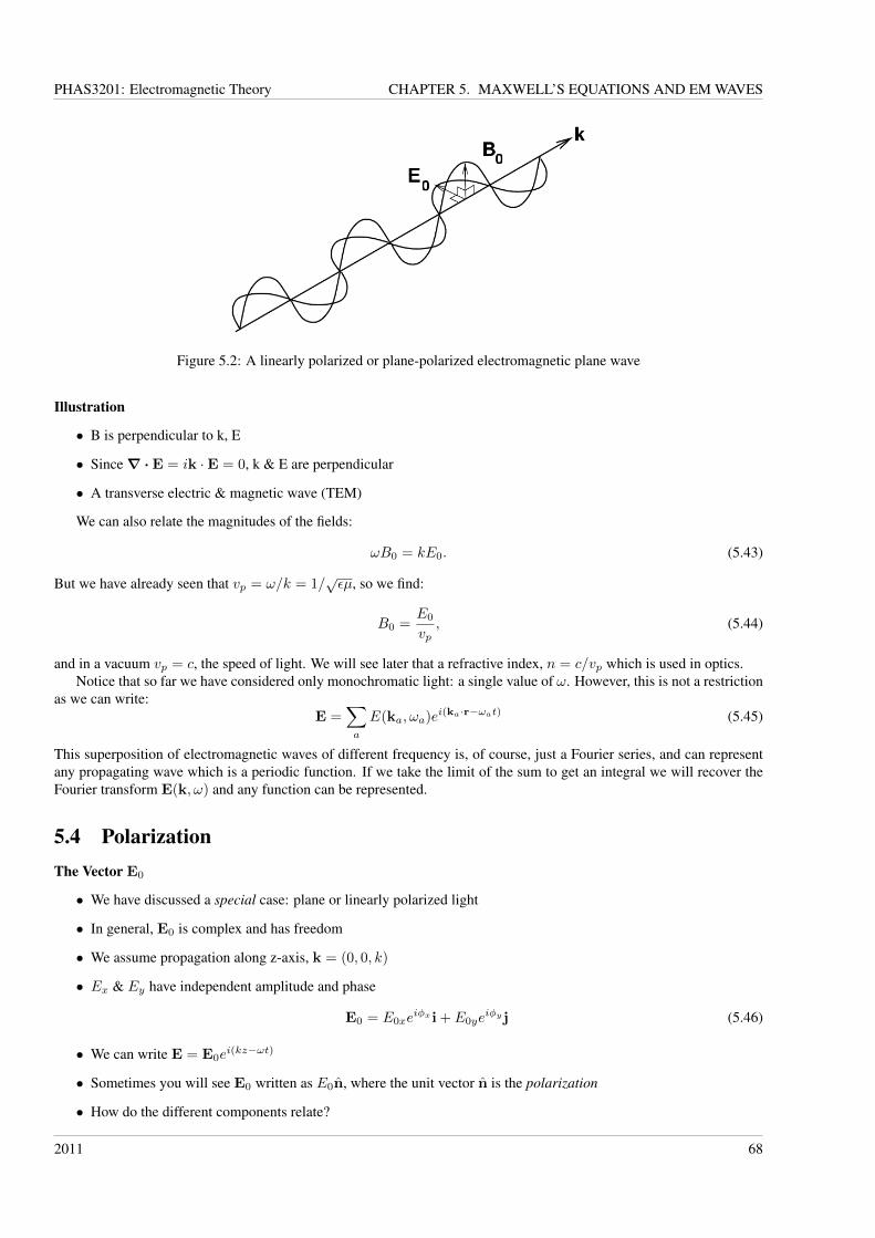
PHAS3201: Electromagnetic Theory CHAPTER 5. MAXWELL’S EQUATIONS AND EM WAVES
Figure 5.2: A linearly polarized or plane-polarized electromagnetic plane wave
Illustration
• B is perpendicular to k, E
• Since∇ ·E = ik ·E = 0, k & E are perpendicular
• A transverse electric & magnetic wave (TEM)
We can also relate the magnitudes of the fields:
ωB0 = kE0. (5.43)
But we have already seen that vp = ω/k = 1/√εµ, so we find:
B0 =E0
vp, (5.44)
and in a vacuum vp = c, the speed of light. We will see later that a refractive index, n = c/vp which is used in optics.Notice that so far we have considered only monochromatic light: a single value of ω. However, this is not a restriction
as we can write:E =
∑a
E(ka, ωa)ei(ka·r−ωat) (5.45)
This superposition of electromagnetic waves of different frequency is, of course, just a Fourier series, and can representany propagating wave which is a periodic function. If we take the limit of the sum to get an integral we will recover theFourier transform E(k, ω) and any function can be represented.
5.4 PolarizationThe Vector E0
• We have discussed a special case: plane or linearly polarized light
• In general, E0 is complex and has freedom
• We assume propagation along z-axis, k = (0, 0, k)
• Ex & Ey have independent amplitude and phase
E0 = E0xeiφx i + E0ye
iφy j (5.46)
• We can write E = E0ei(kz−ωt)
• Sometimes you will see E0 written as E0n, where the unit vector n is the polarization
• How do the different components relate?
2011 68
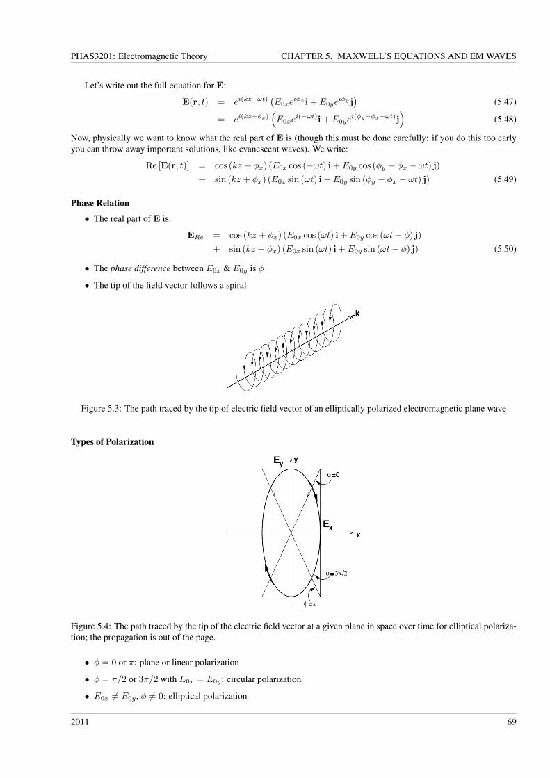
PHAS3201: Electromagnetic Theory CHAPTER 5. MAXWELL’S EQUATIONS AND EM WAVES
Let’s write out the full equation for E:
E(r, t) = ei(kz−ωt)(E0xe
iφx i + E0yeiφy j
)(5.47)
= ei(kz+φx)(E0xe
i(−ωt)i + E0yei(φy−φx−ωt)j
)(5.48)
Now, physically we want to know what the real part of E is (though this must be done carefully: if you do this too earlyyou can throw away important solutions, like evanescent waves). We write:
Re [E(r, t)] = cos (kz + φx) (E0x cos (−ωt) i + E0y cos (φy − φx − ωt) j)+ sin (kz + φx) (E0x sin (ωt) i− E0y sin (φy − φx − ωt) j) (5.49)
Phase Relation
• The real part of E is:
ERe = cos (kz + φx) (E0x cos (ωt) i + E0y cos (ωt− φ) j)
+ sin (kz + φx) (E0x sin (ωt) i + E0y sin (ωt− φ) j) (5.50)
• The phase difference between E0x & E0y is φ
• The tip of the field vector follows a spiral
Figure 5.3: The path traced by the tip of electric field vector of an elliptically polarized electromagnetic plane wave
Types of Polarization
Figure 5.4: The path traced by the tip of the electric field vector at a given plane in space over time for elliptical polariza-tion; the propagation is out of the page.
• φ = 0 or π: plane or linear polarization
• φ = π/2 or 3π/2 with E0x = E0y: circular polarization
• E0x 6= E0y , φ 6= 0: elliptical polarization
2011 69
PHAS3201: Electromagnetic Theory CHAPTER 5. MAXWELL’S EQUATIONS AND EM WAVES
Types
• If E0x 6= E0y for plane polarization, then the plane is at an angle θ = tan−1 (Ey0/Ex0)
• Unpolarised light has the polarization varying randomly with time (only possible for spectral continuum)
• “Ordinary” light sources (e.g. light bulb, sun) give this
• Partially polarized light is a mix of specific kinds, or light which has had a plane imposed (e.g. using Polaroid filter)
• Basic property is the relation of the x and y vectors in the field
2011 70
PHAS3201: Electromagnetic Theory CHAPTER 6. REFLECTION & REFRACTION
Chapter 6
Reflection and Refraction at a PlaneDielectric Surface
6.1 Refractive Index
6.1.1 Origin• Why do materials have a refractive index?
• We have stated that n = c/vp
• In our solution for plane waves, we considered only vacuum
• We will consider two cases with media:
- A non-conducting dielectric (εr)
- A conducting system (briefly)
• Refractive index comes directly from Maxwell’s equations
Let’s start with Ampère’s law, in a linear conducting medium of conductivity g (we can always set this to zero laterto recover a dielectric):
∇×H = J +∂D
∂t(6.1)
J = gE (6.2)
Let’s also assume that we can write the electric displacement and the magnetic intensity as plane waves, with a phasebetween them:
D = D0 exp i (k · r− ωt) (6.3)H = H0 exp i (k · r− ωt+ φ) (6.4)
When these are substituted into Ampère’s law, using standard manipulations first, and then asserting linear, isotropicmedia (B = µ0H, µ ≈ 1 for most linear media, and D = εrε0E) we can write:
ik×H0 = −iωD0 + gE0 (6.5)−k×H0 = ωD0 + igE0 (6.6)k×H0 = −ωD0 − igE0 (6.7)
k× B0
µ0= −ωεrε0E0 − igE0 (6.8)
k×B0 = − ωc2
(εr + i
g
ε0ω
)E0, (6.9)
2011 71
PHAS3201: Electromagnetic Theory CHAPTER 6. REFLECTION & REFRACTION
with µ0ε0 = 1/c2. Looking back to our solution for plane waves in vacuum, we would have seen k × B0 = − ωc2 εrE0
with εr = 1. We can write:
ε = εr + ig
ε0ω(6.10)
k×B0 = − ωc2εE0 (6.11)
We will assume that k ·E = 0 (i.e., that∇·E = 0) and Eis transverse. This is true for a dielectric with no free chargeor a low frequency wave in a conductor where free charges disperse rapidly. There can be significant local accumulationof free charges, for example in a conductor with high frequency waves or certain modes of oscillation in a plasma.
6.1.2 Phase velocityNow, using Faraday’s law on our fields, we can write:
k×E0 = ωB0 (6.12)k× (k×E0) = ωk×B0 (6.13)
(k ·E0)k− k2E0 = −ω2
c2εE0 (6.14)
• We see, finally, that:
k2 = εω2
c2(6.15)
• But the phase velocity,vp =
ω
k=
c√ε
=c
n.
• Note that this means k = nω/c
• What about the two cases?
- A dielectric simply has n =√εr
- A conducting system has a complex dielectric constant and refractive index
• So the refractive index comes directly from the dielectric constant
6.2 Reflection & Refraction
6.2.1 Geometry• We have incident, refracted and reflected waves:
E(r, t) = E0 exp i (k · r− ωt)E′(r, t) = E′0 exp i (k′ · r− ωt)E′′(r, t) = E′′0 exp i (k′′ · r− ωt)
• Phases in prefactors
Consider the boundary region: what will happen to E(r, t), E′(r, t) and E′′(r, t) if we move from r to r+d? We canwrite:
E(r + d, t) = E(r, t) exp i (k · d) (6.16)E′(r + d, t) = E′(r, t) exp i (k′ · d) (6.17)E′′(r + d, t) = E′′(r, t) exp i (k′′ · d) (6.18)
In other words, there is only a change of phase. Now, we know that there are boundary conditions of some kind at theinterface, by definition. We can get quite a long way just with this assumption. The whole of electromagnetism is assumed
2011 72
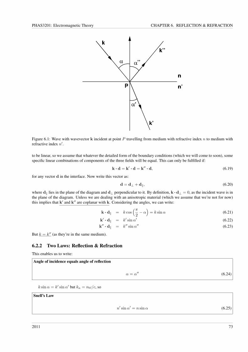
PHAS3201: Electromagnetic Theory CHAPTER 6. REFLECTION & REFRACTION
Figure 6.1: Wave with wavevector k incident at point P travelling from medium with refractive index n to medium withrefractive index n′.
to be linear, so we assume that whatever the detailed form of the boundary conditions (which we will come to soon), somespecific linear combinations of components of the three fields will be equal. This can only be fulfilled if:
k · d = k′ · d = k′′ · d, (6.19)
for any vector d in the interface. Now write this vector as:
d = d⊥ + d‖, (6.20)
where d‖ lies in the plane of the diagram and d⊥ perpendicular to it. By definition, k ·d⊥ = 0, as the incident wave is inthe plane of the diagram. Unless we are dealing with an anisotropic material (which we assume that we’re not for now)this implies that k′ and k′′ are coplanar with k. Considering the angles, we can write:
k · d‖ = k cos(π
2− α
)= k sinα (6.21)
k′ · d‖ = k′ sinα′ (6.22)k′′ · d‖ = k′′ sinα′′ (6.23)
But k = k′′ (as they’re in the same medium).
6.2.2 Two Laws: Reflection & RefractionThis enables us to write:
Angle of incidence equals angle of reflection
α = α′′ (6.24)
k sinα = k′ sinα′ but kn = nω/c, so
Snell’s Law
n′ sinα′ = n sinα (6.25)
2011 73
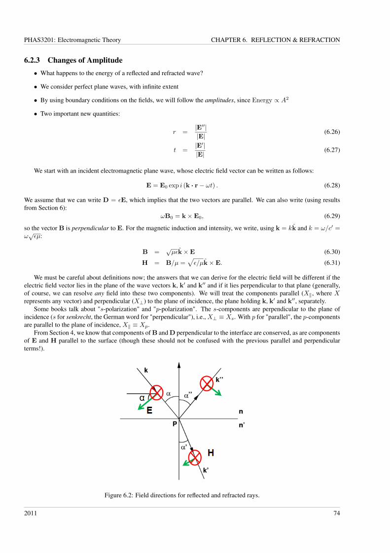
PHAS3201: Electromagnetic Theory CHAPTER 6. REFLECTION & REFRACTION
6.2.3 Changes of Amplitude• What happens to the energy of a reflected and refracted wave?
• We consider perfect plane waves, with infinite extent
• By using boundary conditions on the fields, we will follow the amplitudes, since Energy ∝ A2
• Two important new quantities:
r =|E′′||E|
(6.26)
t =|E′||E|
(6.27)
We start with an incident electromagnetic plane wave, whose electric field vector can be written as follows:
E = E0 exp i (k · r− ωt) . (6.28)
We assume that we can write D = εE, which implies that the two vectors are parallel. We can also write (using resultsfrom Section 6):
ωB0 = k×E0, (6.29)
so the vector B is perpendicular to E. For the magnetic induction and intensity, we write, using k = kk and k = ω/c′ =ω√εµ:
B =√µεk×E (6.30)
H = B/µ =√ε/µk×E. (6.31)
We must be careful about definitions now; the answers that we can derive for the electric field will be different if theelectric field vector lies in the plane of the wave vectors k, k′ and k′′ and if it lies perpendicular to that plane (generally,of course, we can resolve any field into these two components). We will treat the components parallel (X‖, where Xrepresents any vector) and perpendicular (X⊥) to the plane of incidence, the plane holding k, k′ and k′′, separately.
Some books talk about "s-polarization" and "p-polarization". The s-components are perpendicular to the plane ofincidence (s for senkrecht, the German word for "perpendicular"), i.e.,X⊥ ≡ Xs. With p for "parallel", the p-componentsare parallel to the plane of incidence, X‖ ≡ Xp.
From Section 4, we know that components of B and D perpendicular to the interface are conserved, as are componentsof E and H parallel to the surface (though these should not be confused with the previous parallel and perpendicularterms!).
Figure 6.2: Field directions for reflected and refracted rays.
2011 74
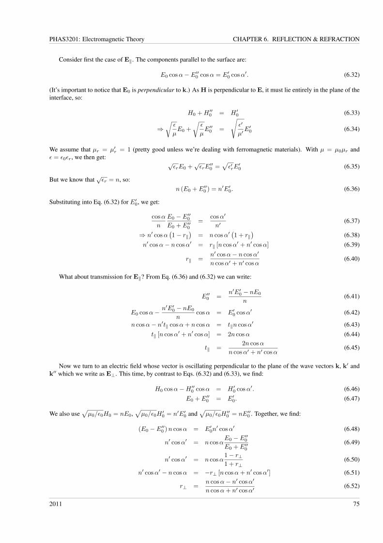
PHAS3201: Electromagnetic Theory CHAPTER 6. REFLECTION & REFRACTION
Consider first the case of E‖. The components parallel to the surface are:
E0 cosα− E′′0 cosα = E′0 cosα′. (6.32)
(It’s important to notice that E0 is perpendicular to k.) As H is perpendicular to E, it must lie entirely in the plane of theinterface, so:
H0 +H ′′0 = H ′0 (6.33)
⇒√ε
µE0 +
√ε
µE′′0 =
√ε′
µ′E′0 (6.34)
We assume that µr = µ′r = 1 (pretty good unless we’re dealing with ferromagnetic materials). With µ = µ0µr andε = ε0εr, we then get:
√εrE0 +
√εrE
′′0 =
√ε′rE
′0 (6.35)
But we know that√εr = n, so:
n (E0 + E′′0 ) = n′E′0. (6.36)
Substituting into Eq. (6.32) for E′0, we get:
cosα
n
E0 − E′′0E0 + E′′0
=cosα′
n′(6.37)
⇒ n′ cosα(1− r‖
)= n cosα′
(1 + r‖
)(6.38)
n′ cosα− n cosα′ = r‖ [n cosα′ + n′ cosα] (6.39)
r‖ =n′ cosα− n cosα′
n cosα′ + n′ cosα(6.40)
What about transmission for E‖? From Eq. (6.36) and (6.32) we can write:
E′′0 =n′E′0 − nE0
n(6.41)
E0 cosα− n′E′0 − nE0
ncosα = E′0 cosα′ (6.42)
n cosα− n′t‖ cosα+ n cosα = t‖n cosα′ (6.43)t‖ [n cosα′ + n′ cosα] = 2n cosα (6.44)
t‖ =2n cosα
n cosα′ + n′ cosα(6.45)
Now we turn to an electric field whose vector is oscillating perpendicular to the plane of the wave vectors k, k′ andk′′ which we write as E⊥. This time, by contrast to Eqs. (6.32) and (6.33), we find:
H0 cosα−H ′′0 cosα = H ′0 cosα′. (6.46)E0 + E′′0 = E′0. (6.47)
We also use√µ0/ε0H0 = nE0,
√µ0/ε0H
′0 = n′E′0 and
√µ0/ε0H
′′0 = nE′′0 . Together, we find:
(E0 − E′′0 )n cosα = E′0n′ cosα′ (6.48)
n′ cosα′ = n cosαE0 − E′′0E0 + E′′0
(6.49)
n′ cosα′ = n cosα1− r⊥1 + r⊥
(6.50)
n′ cosα′ − n cosα = −r⊥ [n cosα+ n′ cosα′] (6.51)
r⊥ =n cosα− n′ cosα′
n cosα+ n′ cosα′(6.52)
2011 75
PHAS3201: Electromagnetic Theory CHAPTER 6. REFLECTION & REFRACTION
Finally we consider transmission for the perpendicular case:
[E0 − (E′0 − E0)]n cosα = E′0n′ cosα′ (6.53)
⇒ 2E0 − E′0 = E′0n′ cosα′
n cosα(6.54)
2n cosα = t⊥ (n′ cosα′ + n cosα) (6.55)
t⊥ =2n cosα
n′ cosα′ + n cosα(6.56)
6.2.4 Fresnel Relations• These are called the Fresnel Relations
Fresnel Relations
r‖ =n′ cosα− n cosα′
n′ cosα+ n cosα′(6.57)
r⊥ =n cosα− n′ cosα′
n cosα+ n′ cosα′(6.58)
t‖ =2n cosα
n′ cosα+ n cosα′(6.59)
t⊥ =2n cosα
n cosα+ n′ cosα′(6.60)
• They tell us about amplitudes of waves
• For power (or intensity) we need their square
We can see this by considering an electromagnetic wave with:
H =B
µ=
√ε
µk×E. (6.61)
We will see later that the energy transmitted in an electromagnetic wave is proportional to E ×H, which (here) will beproportional to
√ε/µE2
0 . So the reflection and transmission coefficients are proportional to the square root of the power.It will be useful to rewrite r‖ and r⊥ in a rather different form. We will not derive this form: it’s basic manipulation,
though quite long.
r‖ =tan (α− α′)tan (α+ α′)
(6.62)
r⊥ =sin (α− α′)sin (α+ α′)
(6.63)
6.3 Special AnglesThere are two particularly important angles where interesting things happen to the reflection and transmission coefficients.
6.3.1 Brewster Angle• At some point, r‖ → 0 but r⊥ 6= 0
• This is the Brewster angle, αB , sometimes αp
• All the power of the incident E‖ wave goes into the refracted wave
• But in general the incident wave will have a E⊥ component
2011 76
PHAS3201: Electromagnetic Theory CHAPTER 6. REFLECTION & REFRACTION
Figure 6.3: The Brewster angle.
• Thus, the reflected light will be polarized perpendicular to the plane of incidence
If r‖ = 0 then we can write the Fresnel relation as:
n′ cosαB = n cosα′, (6.64)
where αB is the Brewster angle. But Snell’s law also tells us that n′ sinα′ = n sinαB .Now, using our other expression for r‖, tan(α−α′)/ tan(α+α′), we can see that if α+α′ = π
2 then tan(α+α′)→∞so r‖ = 0. Then α′ = π
2 − αB . Substituting into Snell’s law we see:
n′ sin(π
2− αB
)= n sinαB (6.65)
n′ cosαB = n sinαB (6.66)(6.67)
• The final result is:
Brewster Angle
αB = tan−1
(n′
n
)(6.68)
• Many shiny dielectrics (paint, wet roads etc) have n′/nair ∼ 1.5, so αB ≈ 50 to 60◦
• Notice that r‖ changes sign, so direction of reflected vectors changes
6.3.2 Critical Angle• Is there a situation where the transmission goes to zero?
• The trivial solution is α = π/2, which explains glancing reflection from still lakes and glass
• If n > n′, Snell’s law gives:
sinα′ =n
n′sinα (6.69)
• There will be some angle α above which sinα′ > 1, which is unphysical
2011 77
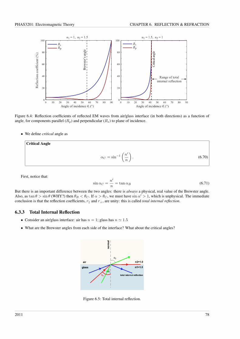
PHAS3201: Electromagnetic Theory CHAPTER 6. REFLECTION & REFRACTION
Figure 6.4: Reflection coefficients of reflected EM waves from air/glass interface (in both directions) as a function ofangle, for components parallel (Rp) and perpendicular (Rs) to plane of incidence.
• We define critical angle as
Critical Angle
αC = sin−1
(n′
n
). (6.70)
First, notice that:
sinαC =n′
n= tanαB (6.71)
But there is an important difference between the two angles: there is always a physical, real value of the Brewster angle.Also, as tan θ > sin θ (WHY?) then θB < θC . If α > θC , we must have sinα′ > 1, which is unphysical. The immediateconclusion is that the reflection coefficients, r‖ and r⊥, are unity: this is called total internal reflection.
6.3.3 Total Internal Reflection• Consider an air/glass interface: air has n = 1; glass has n ' 1.5
• What are the Brewster angles from each side of the interface? What about the critical angles?
Figure 6.5: Total internal reflection.
2011 78
PHAS3201: Electromagnetic Theory CHAPTER 6. REFLECTION & REFRACTION
6.3.4 IntensitiesBut what is wrong with asserting that sin θ > 1? It would imply that cos θ =
√1− sin2 θ would be imaginary. Let’s
assume that this is reasonable, and write:cosα′ = iS, (6.72)
with S a real, positive number. What will this do to the reflection coefficients? They will have the form:
r =a− iba+ ib
=ρ exp (−iφ)
ρ exp (+iφ)= exp (−2iφ) (6.73)
The magnitude of this will always be one (as expected from before), meaning that all the power will be reflected, but itwill insert a phase shift (as E′′0 /E0 will be complex).
Now, the phase for a plane wave below the interface, when the angle of incidence exceeds the critical angle, withsinα′ = n
n′ sinα - Snell’s Law, and using Eq. 6.72, is given by:
k′ · r = k′ sinα′x+ k′ cosα′z (6.74)
= k′n
n′sinαx+ ik′Sz (6.75)
Evanescent Waves
• Using Eq. 6.75, we write for the electric field below the interface:
E′ = E′0 exp i (k′ · r− ωt) (6.76)
= E′0 exp i(k′n
n′sinαx+ ik′Sz − ωt
)(6.77)
= E′0 exp i (ik′Sz) exp i(k′n
n′sinαx− ωt
)(6.78)
E′ = E′0 exp (−k′Sz) exp i (k′ (n/n′) sinαx− ωt) (6.79)
• This is a travelling wave along x which decays exponentially with z
• It is called an evanescent wave
• If another piece of material is brought up below the interface, a new wave can be excited, driven by the evanescentwave
2011 79
PHAS3201: Electromagnetic Theory CHAPTER 6. REFLECTION & REFRACTION
2011 80
PHAS3201: Electromagnetic Theory CHAPTER 7. WAVES IN CONDUCTING MEDIA
Chapter 7
Waves in Conducting Media
7.1 Conductors
7.1.1 Origins• All effects stem from the wave equation:
∇2E− gµ∂E∂t− εµ∂
2E
∂t2= 0 (7.1)
• In a conducting medium, J = gE, with conductance g
• Now see the effect on the plane wave:E = E0 exp i (k · r− ωt) (7.2)
For the various components we can write:
∇2E = −k2E (7.3)∂E
∂t= −iωE (7.4)
∂2E
∂t2= −ω2E (7.5)
Combining these, we can form the following equation:
−k2 + iωgµ+ ω2µε = 0 (7.6)
7.1.2 Dispersion Relation• The dispersion relation is:
k2 = µεω2
(1 +
ig
εω
)(7.7)
• We get a variation of k (or λ = 2π/k) with ω
• Remember that vg = dω/dk and vp = ω/k
• g → 0: poor conductor, so k2 = µεω2 and vp = vg
7.1.3 Good Conductors• If g >> εω, we have a good conductor, and
k2 ≈ iµgω ⇒ k = +√iµgω (7.8)
2011 81
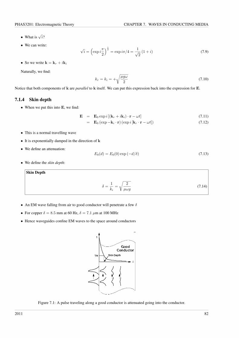
PHAS3201: Electromagnetic Theory CHAPTER 7. WAVES IN CONDUCTING MEDIA
• What is√i?
• We can write:√i =
(exp i
π
2
) 12
= exp iπ/4 =1√2
(1 + i) (7.9)
• So we write k = kr + iki
Naturally, we find:
kr = ki = +
√µgω
2(7.10)
Notice that both components of k are parallel to k itself. We can put this expression back into the expression for E.
7.1.4 Skin depth• When we put this into E, we find:
E = E0 exp i [(kr + iki) · r− ωt] (7.11)= E0 (exp−ki · r) (exp i [kr · r− ωt]) (7.12)
• This is a normal travelling wave
• It is exponentially damped in the direction of k
• We define an attenuation:E0(d) = E0(0) exp (−d/δ) (7.13)
• We define the skin depth:
Skin Depth
δ =1
ki=
√2
µωg(7.14)
• An EM wave falling from air to good conductor will penetrate a few δ
• For copper δ = 8.5 mm at 60 Hz, δ = 7.1 µm at 100 MHz
• Hence waveguides confine EM waves to the space around conductors
Figure 7.1: A pulse traveling along a good conductor is attenuated going into the conductor.
2011 82
PHAS3201: Electromagnetic Theory CHAPTER 7. WAVES IN CONDUCTING MEDIA
Neither the electric field (E) nor the magnetic field (H) penetrate far into a "good" conductor. The point where thesefields are reduced by a factor of 1/e ≈ 1/2.71 is called the skin depth. Fig. 7.1 shows a good conductor and how a pulsetraveling along this conductor is attenuated going into the conductor.
Skin depth is dependent on the type of metal in the conductor and the frequency fields applied to the conductor. Athigh frequencies the skin depth is very shallow, and the field are often considered to be 0 in a few millimeters. A generalrule is that at five times the skin depth the fields can be considered to be 0 (the actual value is (1/e)5 = 0.00674, whichis indeed quite small).
Skin depth is important in many pulsed power applications because it changes the effective resistance in a conductor,and that only the surface of the conductor matters.
7.2 Reflection At Metal SurfaceWe start with the refractive index, n, which can be (and will be here!) complex.
7.2.1 Refractive Index• We know that n = ck/ω
• If we substitute in from the results above, assuming µ = µ0 we get:
n =c
ω
√µgω
(1 + i√
2
)=
√g
2ωε0(1 + i) (7.15)
• A “good” conductor, as defined earlier, has g >> εω, so |n| >> 1
Consider normal incidence at a metal surface:There are two ways to get the result that we want. First, consider simply the Fresnel relation for α = 0◦:
r⊥ =n cosα− n′ cosα′
n cosα+ n′ cosα′(7.16)
r⊥ (α = 0◦) =n− n′
n+ n′(7.17)
If we are coming from air or vacuum to the metal, n = 1. Then in the limit of a good conductor, n′ � 1, we have:
r⊥ =1− n′
1 + n′≈ −1 (7.18)
This tells us that, provided we have a large conductivity and are not at high frequencies, the reflected amplitude has thesame magnitude as the incident amplitude. However, this is not true at lower frequencies (e.g., optical frequencies, wherecoloured reflections from metal surfaces show that the amplitudes are changing; note that there are a number of causes forthe colour of metals which is a complex subject!).
The second way to find this result is simply using the boundary conditions that we derived on the fields. Taking asmall loop which lies either side of the interface (ABCD as before), continuity of tangential components tells us that:
E0 + E′′0 = E′0 and H0 −H ′′0 = H ′0 (7.19)
The minus sign on H ′′0 ensures that the reflected wave goes in the opposite direction to the incoming wave, and reversesthe direction of energy flow. If we assume that µ = µ0, and shrink the sides of the small loop so that we can neglect thefree currents in the metal (which penetrate a few skin depths), then B0 −B′′0 = B′0. We also know that B0 = E0k/ω, so,with ω/k = c for air/vacuum:
k
ωE0 −
k
ωE′′0 =
k′
ωE′0 (7.20)
E0 − E′′0 =ck′
ωE′0 =
c
v′pE′0 = n′E′0 (7.21)
If we eliminate E′0 between equations, we get, as before with before (Eq. 7.18):
E0 − E′′0 = n′ (E0 + E′′0 ) (7.22)
r⊥ =E′′0E0
=1− n′
1 + n′(7.23)
2011 83
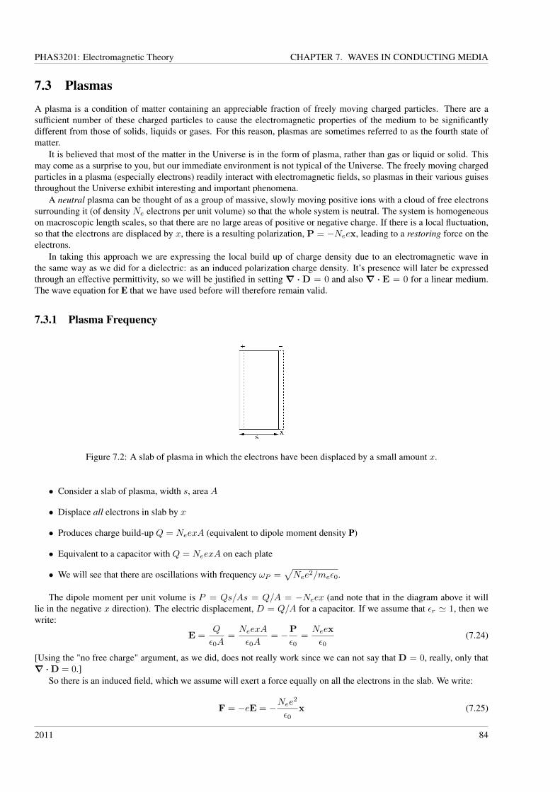
PHAS3201: Electromagnetic Theory CHAPTER 7. WAVES IN CONDUCTING MEDIA
7.3 Plasmas
A plasma is a condition of matter containing an appreciable fraction of freely moving charged particles. There are asufficient number of these charged particles to cause the electromagnetic properties of the medium to be significantlydifferent from those of solids, liquids or gases. For this reason, plasmas are sometimes referred to as the fourth state ofmatter.
It is believed that most of the matter in the Universe is in the form of plasma, rather than gas or liquid or solid. Thismay come as a surprise to you, but our immediate environment is not typical of the Universe. The freely moving chargedparticles in a plasma (especially electrons) readily interact with electromagnetic fields, so plasmas in their various guisesthroughout the Universe exhibit interesting and important phenomena.
A neutral plasma can be thought of as a group of massive, slowly moving positive ions with a cloud of free electronssurrounding it (of density Ne electrons per unit volume) so that the whole system is neutral. The system is homogeneouson macroscopic length scales, so that there are no large areas of positive or negative charge. If there is a local fluctuation,so that the electrons are displaced by x, there is a resulting polarization, P = −Neex, leading to a restoring force on theelectrons.
In taking this approach we are expressing the local build up of charge density due to an electromagnetic wave inthe same way as we did for a dielectric: as an induced polarization charge density. It’s presence will later be expressedthrough an effective permittivity, so we will be justified in setting∇ ·D = 0 and also∇ · E = 0 for a linear medium.The wave equation for E that we have used before will therefore remain valid.
7.3.1 Plasma Frequency
Figure 7.2: A slab of plasma in which the electrons have been displaced by a small amount x.
• Consider a slab of plasma, width s, area A
• Displace all electrons in slab by x
• Produces charge build-up Q = NeexA (equivalent to dipole moment density P)
• Equivalent to a capacitor with Q = NeexA on each plate
• We will see that there are oscillations with frequency ωP =√Nee2/meε0.
The dipole moment per unit volume is P = Qs/As = Q/A = −Neex (and note that in the diagram above it willlie in the negative x direction). The electric displacement, D = Q/A for a capacitor. If we assume that εr ' 1, then wewrite:
E =Q
ε0A=NeexA
ε0A= −P
ε0=Neex
ε0(7.24)
[Using the "no free charge" argument, as we did, does not really work since we can not say that D = 0, really, only that∇ ·D = 0.]
So there is an induced field, which we assume will exert a force equally on all the electrons in the slab. We write:
F = −eE = −Nee2
ε0x (7.25)
2011 84
PHAS3201: Electromagnetic Theory CHAPTER 7. WAVES IN CONDUCTING MEDIA
If the electrons are free to move under the action of this force, we should recognize it as giving the equation for simpleharmonic motion. Applying Newton’s Second Law:
d2
dt2x = −Nee
2
meε0x (7.26)
This allows us to identify the plasma frequency, ωP :
Plasma Frequency
ωP =
√Nee2
meε0, (7.27)
If we consider a charge density Ne = 1018 electrons per cubic metre, then the frequency is ωP ' 5.7× 10¹⁰s−1.
7.3.2 Dispersion• For an EM wave in a plasma, how does k depend on ω?
• Collisions between electrons and ions are assumed infrequent
• For a high frequency wave, consider free electrons
• (only for a few cycles)
• Compare to a metal where ohmic collisions dissipate energy
• We will find:
k2 =ω2
c2
(1−
ω2p
ω2
)(7.28)
Derivation: Let us assume that we have a plane wave:
E(r, t) = E0 exp i (k · r− ωt) (7.29)
The force on an electron in the plasma will be:
F = mdv
dt= −e (E(r, t) + v ×B(r, t)) (7.30)
However, we can neglect the contribution from the magnetic field in a non-relativistic plasma. We know that B0 = E0/vp(from Faraday’s Law, for instance) so that the ratio of the two parts of the force in Eq. (7.30) is:
|v ×B||E|
=v
vp(7.31)
But vp ' c >> v (as we’re in a non-relativistic plasma) so that vB0 << E0, and the magnetic term can be neglected.So we now have:
mdv
dt= −eE(r, t) = −eE0 exp i (k · r− ωt) (7.32)
This is simple enough to integrate directly with respect to time:∫dv
dtdt = − e
mE0 exp ik · r
∫exp (−iωt) dt (7.33)
⇒ v = − ei
ωmE (7.34)
The electrons moving together as a group with this velocity gives a current, with a current density:
J = −Neev = i
(Nee
2
mω
)E (7.35)
2011 85
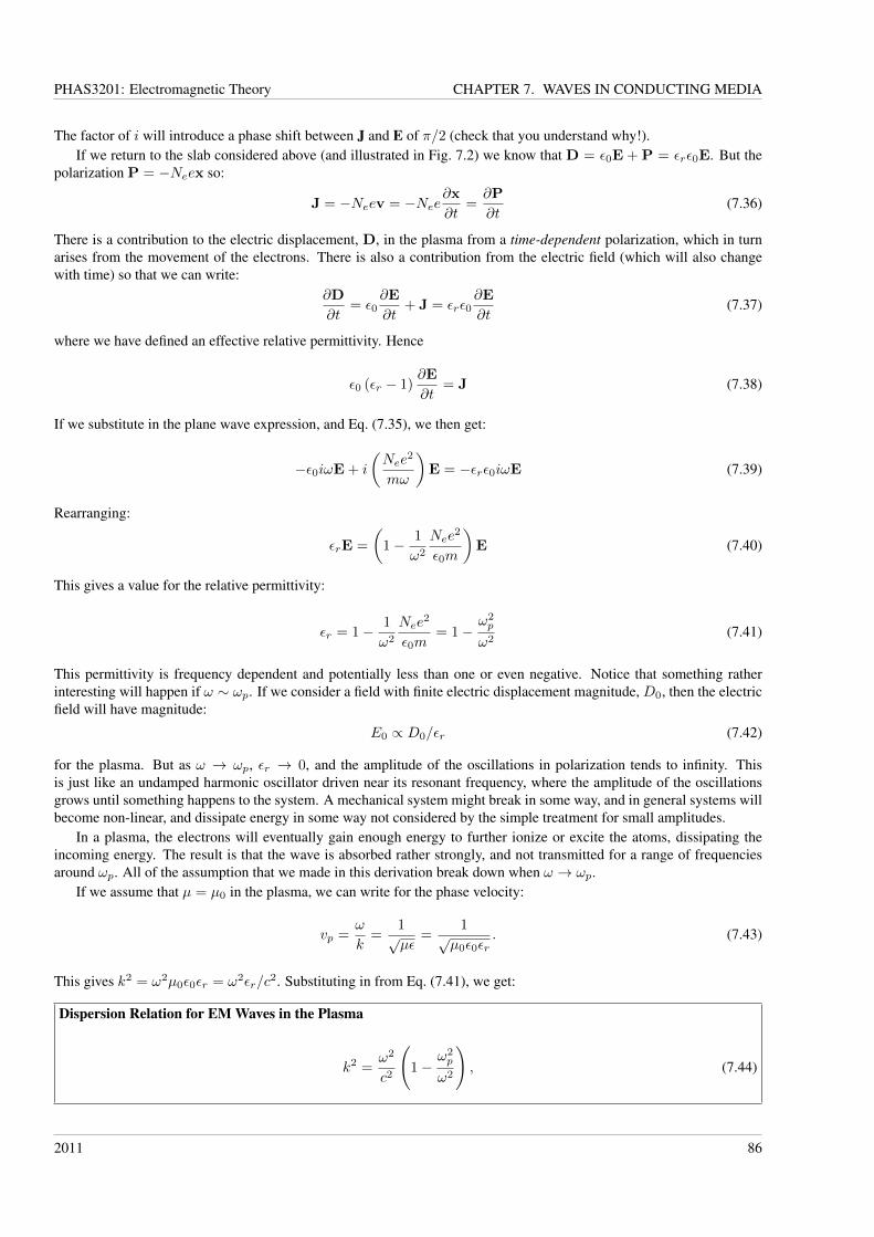
PHAS3201: Electromagnetic Theory CHAPTER 7. WAVES IN CONDUCTING MEDIA
The factor of i will introduce a phase shift between J and E of π/2 (check that you understand why!).If we return to the slab considered above (and illustrated in Fig. 7.2) we know that D = ε0E + P = εrε0E. But the
polarization P = −Neex so:
J = −Neev = −Nee∂x
∂t=∂P
∂t(7.36)
There is a contribution to the electric displacement, D, in the plasma from a time-dependent polarization, which in turnarises from the movement of the electrons. There is also a contribution from the electric field (which will also changewith time) so that we can write:
∂D
∂t= ε0
∂E
∂t+ J = εrε0
∂E
∂t(7.37)
where we have defined an effective relative permittivity. Hence
ε0 (εr − 1)∂E
∂t= J (7.38)
If we substitute in the plane wave expression, and Eq. (7.35), we then get:
−ε0iωE + i
(Nee
2
mω
)E = −εrε0iωE (7.39)
Rearranging:
εrE =
(1− 1
ω2
Nee2
ε0m
)E (7.40)
This gives a value for the relative permittivity:
εr = 1− 1
ω2
Nee2
ε0m= 1−
ω2p
ω2(7.41)
This permittivity is frequency dependent and potentially less than one or even negative. Notice that something ratherinteresting will happen if ω ∼ ωp. If we consider a field with finite electric displacement magnitude, D0, then the electricfield will have magnitude:
E0 ∝ D0/εr (7.42)
for the plasma. But as ω → ωp, εr → 0, and the amplitude of the oscillations in polarization tends to infinity. Thisis just like an undamped harmonic oscillator driven near its resonant frequency, where the amplitude of the oscillationsgrows until something happens to the system. A mechanical system might break in some way, and in general systems willbecome non-linear, and dissipate energy in some way not considered by the simple treatment for small amplitudes.
In a plasma, the electrons will eventually gain enough energy to further ionize or excite the atoms, dissipating theincoming energy. The result is that the wave is absorbed rather strongly, and not transmitted for a range of frequenciesaround ωp. All of the assumption that we made in this derivation break down when ω → ωp.
If we assume that µ = µ0 in the plasma, we can write for the phase velocity:
vp =ω
k=
1√µε
=1
√µ0ε0εr
. (7.43)
This gives k2 = ω2µ0ε0εr = ω2εr/c2. Substituting in from Eq. (7.41), we get:
Dispersion Relation for EM Waves in the Plasma
k2 =ω2
c2
(1−
ω2p
ω2
), (7.44)
2011 86
PHAS3201: Electromagnetic Theory CHAPTER 7. WAVES IN CONDUCTING MEDIA
Phase/Group Velocities
• Consider a wave with ω > ωp: then k2 > 0, so k is real and there is no attenuation
• If ω < ωp, k2 < 0 and we have absorption of energy and damping over some attenuation length, L.
• Let us consider the phase and group velocities, which are defined as:
vp =ω
k(7.45)
vg =dω
dk(7.46)
Now using the expression for the dispersion relation, Eq. (7.28), and differentiating, we find:
2ωdω
dk= 2kc2 (7.47)
⇒ vg =k
ωc2 = c2/vp (7.48)
We find:vpvg = c2 (7.49)
So either both velocities are equal to c, or vp > c. But this is all right: information and energy are transmitted at the groupvelocity. We can see why the phase velocity is greater than c by considering the refractive index, n:
n = c/vp (7.50)
n2 =c2k2
ω2= 1−
ω2p
ω2(7.51)
So n < 1 and vp > c.An application: radio waves in the ionosphere.
2011 87

PHAS3201: Electromagnetic Theory CHAPTER 7. WAVES IN CONDUCTING MEDIA
2011 88
PHAS3201: Electromagnetic Theory CHAPTER 8. ENERGY FLOW AND THE POYNTING VECTOR
Chapter 8
Energy Flow and the Poynting Vector
8.1 Poynting’s TheoremWe will be looking at the energy flow due to an electromagnetic wave.
8.1.1 Energy Densities• Recall the energy densities in static fields:
Ue =1
2E ·D (8.1)
Um =1
2B ·H (8.2)
• Consider EM energy dissipated via J in a medium
• Rate of work (power, P ) done is:F · v = qE · v = E · qv (8.3)
• This is just E · J per unit volume
We will analyze the flow and storage of energy.Notice that if J is perpendicular to E, there will be no energy dissipation. This is equivalent to a body in orbit, where
the force is always perpendicular to the velocity (unless we include dissipation!) and there is no work done. It’s alsouseful to think about a ball thrown upwards in a parabolic trajectory moving under the gravitational force. The rate oftransfer of energy will be negative initially (as the ball slows down), zero at the top of the curve (any velocity will behorizontal) and positive as the ball falls.
Now consider the rate of transfer of energy from EM field to the current in a volume V :
PV =
∫V
J ·Edv (8.4)
(If the medium is one that obeys the law J = gE then we have PV =∫VgE2dv.) Now we use Maxwell’s equations (in
particular Ampère’s law and Faraday’s law) to transform the rate of transfer of energy:
∇×H = J +∂D
∂t(8.5)
⇒ J = ∇×H− ∂D
∂t(8.6)
So in a situation with electric and magnetic fields, we have:
PV =
∫V
dv
{E · ∇×H−E · ∂D
∂t
}(8.7)
2011 89
PHAS3201: Electromagnetic Theory CHAPTER 8. ENERGY FLOW AND THE POYNTING VECTOR
But we can use a theorem from vector calculus to rework this expression:
∇ · (E×H) = H · ∇×E−E · ∇×H (8.8)
Now we can substitute for E · ∇×H, and use Faraday’s law (∇×E = −∂B/∂t) to replace∇×E. This gives:
PV =
∫V
dv
{−∇ · (E×H) + H · ∇×E−E · ∂D
∂t
}(8.9)
= −∫V
dv
{∇ · (E×H) + H · ∂B
∂t+ E · ∂D
∂t
}(8.10)
Assuming that we’re in a linear, isotropic medium, we can write B = µH and D = εE. This also means that:
H · ∂B∂t
=1
2
∂
∂t(H ·B) (8.11)
E · ∂D∂t
=1
2
∂
∂t(D ·E) (8.12)
Remember that the energy densities in magnetic and electric fields were written as 12H ·B and 1
2D ·E respectively. UsingEq. (8.4) for PV we can now write:∫
V
dvJ ·E = −∫V
dv
{∇ · (E×H) +
1
2
∂
∂t(H ·B + E ·D)
}(8.13)
8.1.2 Energy Flow• Finally, we find:
−∫V
dv∇ · (E×H) =∂
∂t
∫V
dv1
2(H ·B + E ·D)
+
∫V
dvJ ·E (8.14)
• The first term on RHS is rate of change with time of stored energy in fields
• The second term on RHS is rate of dissipation of energy
• Define:
Poynting vector
N = E×H (8.15)
The Poynting vector can be thought of as representing the directional energy flux density (the rate of energy transferper unit area, in Wm−2) of an electromagnetic field.
8.1.3 Poynting’s TheoremFirst notice that we can use the divergence theorem to write:∫
V
dv∇ ·N =
∮S
daN · n (8.16)
Here, N · n is the outward energy flux through area element da.
• Assert that∮SdaN · n is the rate of flow of energy through the surface S as EM waves
−∮S
daN · n =
∫V
[∂
∂t
(1
2H ·B +
1
2E ·D
)+ J ·E
]dv (8.17)
2011 90
PHAS3201: Electromagnetic Theory CHAPTER 8. ENERGY FLOW AND THE POYNTING VECTOR
• This cannot be generally proven, but the derivation given above is a good reason for accepting and using N
As an example, let’s consider the energy flow in a plane wave of the usual form E = E0 exp i (k · r− ωt). Then wehave:
H =k×E
µω(8.18)
k
ω=
1
vp=√εµ (8.19)
8.1.4 Average flow
• But E0 ×(k×E0
)= E2
0 k, so:
N =
√ε
µE2
0 k cos2 (k · r− ωt) (8.20)
• This is in the direction of propagation, and varies with time.
• The time average is:
〈N〉 =1
2
√ε
µE2
0 k (8.21)
=1
2< (E×H?) (8.22)
• where the second form is for complex vectors (are the results the same?)
We have used the time average over one period (T = 2π/ω):
ω
2π
∫ 2πω
0
cos2 ωtdt =1
2(8.23)
8.2 Pressure due to EM WavesWhile this derivation/demonstration could be done within the classical realm, it’s easier to do once we recognise that EMwaves are composed of photons. In a radio wave or light beam the energies of individual photons are small and phases arecoherent, so that the classical fields E(r, t) and H(r, t) describe with high precision the behaviour of all these particles.
The classical results involves relating current flow in a conductor to the electric field strength in the wave impingingon a surface, and then finding the Lorentz force acting on that current due to the magnetic field of the wave.
8.2.1 Photons• We know that they have invariant mass m0 = 0 and energy E = hω = hν
• In special relativity, E2 = p2c2 +m20c
4 (more on this later)
• So the momentum of one photon is:
pi =E
c=hν
c(8.24)
The momentum in the wave will be the sum over the photons crossing a unit area in unit time:
p =∑i
pi =1
c
∑i
hνi (8.25)
p =E
c=〈N〉c, (8.26)
2011 91
PHAS3201: Electromagnetic Theory CHAPTER 8. ENERGY FLOW AND THE POYNTING VECTOR
where, in the second equation, we’ve used the expression for energy flow from earlier.If we assume that there is total reflection (e.g. from a metal surface—as will be discussed in the next section of the
lectures) then the change of momentum per unit area per unit time will be, using Eq. 8.21:
∆p = 2〈N〉c
= ε0E20 , (8.27)
which is equal to the pressure on the surface (CHECK DIMENSIONS!). Notice that we’re assuming µr = 1 = εr. If thephotons are absorbed rather than reflected we lose the factor of two.
2011 92
PHAS3201: Electromagnetic Theory CHAPTER 9. EMISSION OF RADIATION
Chapter 9
Emission of Radiation
9.1 Retarded Potentials
We will consider the emission of electromagnetic waves from sources. The retarded potentials describe the scalar orvector potential for electromagnetic fields of a time-varying current or charge distribution. The retardation of the influenceconnecting cause and effect is thereby essential; e.g. the signal takes a finite time, corresponding to the velocity of light, topropagate from the source point of the field to the point where an effect is produced or measured. Indeed, this ultimatelyleads to the study of self-fields, where the motion of a particle (source) due to the fields generated by that same particle iscalculated – sadly, beyond the scope of this course.
To start with, we will solve for the scalar and vector potentials in terms of charge and current densities.
9.1.1 Fields
• How are fields determined by potentials?
• B is easy (from∇ ·B = 0):
B =∇×A (9.1)
• We get E from Faraday’s law:
E = −∇φ− ∂A
∂t(9.2)
• Use these to relate A and φ to J and ρ
Faraday’s law can be rewritten:
∇×E +∂B
∂t= 0 =∇×E +
∂
∂t∇×A
⇒∇×(E +
∂A
∂t
)= 0
The last equality only holds if the fields are continuous. We know that the curl of a gradient is always zero, so wewrite (as we’ve seen before):
E +∂A
∂t= −∇φ (9.3)
E = −∇φ− ∂A
∂t(9.4)
2011 93
PHAS3201: Electromagnetic Theory CHAPTER 9. EMISSION OF RADIATION
If we assume a linear, isotropic medium, then we can write the Ampère-Maxwell equation (∇×H = J + ∂D/∂t), withB = µH and D = εE as:
1
µ∇×B = J + ε
∂E
∂t(9.5)
⇒ 1
µ∇×∇×A + ε
∂
∂t
(∇φ+
∂A
∂t
)= J (9.6)
⇒ −∇2A + εµ∂2A
∂t2+∇ (∇ ·A) + εµ∇∂φ
∂t= µJ (9.7)
where we have used∇× (∇×A) =∇(∇ ·A)−∇2A.But this is rather messy! As we noted in Section III, there is considerable freedom in choosing A, since∇×∇f = 0.
Before, we chose the Coulomb gauge: ∇ ·A = 0.
Summary
• We wish to solve for fields E(r, t) and B(r, t)
• It is easier to work in terms of potentials:
B = ∇×A (9.8)
E = −∇φ− ∂A
∂t(9.9)
• From Maxwell’s equations, we find:
∇2φ +∂
∂t(∇ ·A) = − ρ
ε0(9.10)
−∇2A + εµ∂2A
∂t2+∇ (∇ ·A) + εµ∇∂φ
∂t= µJ (9.11)
• We can use gauges to simplify
9.1.2 Lorentz Condition• We will impose a condition on our potentials:
∇ ·A + εµ∂φ
∂t= 0 (9.12)
• This is known as the Lorentz condition.
• Notice that we can always write A→ A +∇Λ and φ→ φ− ∂Λ/∂t
• So:
∇2Λ− εµ∂2Λ
∂t2= 0 (9.13)
• All potentials belonging to the Lorentz gauge satisfy this condition
9.1.3 Wave Equations• The vector potential now satisfies:
−∇2A + εµ∂2A
∂t2= µJ (9.14)
• The scalar potential can be shown to satisfy:
−∇2φ+ εµ∂2φ
∂t2=ρ
ε(9.15)
2011 94
PHAS3201: Electromagnetic Theory CHAPTER 9. EMISSION OF RADIATION
• How do we solve these equations?
We will consider the solution of the particular integral (which is the hard part!) for the scalar potential first. If thepotential was time independent, then we know that:
φ(r) =1
4πε0
∫V
ρ (r′)
|r− r′|dv′ (9.16)
But this doesn’t (quite) work. In vacuum,
−∇2φ+1
c2∂2φ
∂t2=
ρ
ε0.
We will solve for a point charge at the origin, and integrate over a volume (this is rather close to using a Green’s functiontechnique). So we write:
−∇2φ+1
c2∂2φ
∂t2= 0, (9.17)
except in a small volume ∆v around the origin. If we define a time dependent point charge purely as a mathematicaldevice (because a time-dependent point charge breaks charge conservation), then we can write:∫
∆v
dv
[∇2φ− 1
c2∂2φ
∂t2
]=
1
ε0q(t) (9.18)
For this system, we can immediately see that there must be spherical symmetry, so φ(r) = φ (|r|). We can rewriteEq. (9.17) as:
1
r2
∂
∂r
(r2 ∂φ
∂r
)− 1
c2∂2φ
∂t2= 0 (9.19)
If we wrote φ(r, t) = χ(r, t)/r then this would become:
∂2χ
∂r2− 1
c2∂2χ
∂t2= 0, (9.20)
which is of course just a one-dimensional wave equation. In general, we write:
χ(r, t) = f(r − ct) + g(r + ct) (9.21)
However, we will ignore the second solution as we want a wave which propagates outward with time. Now we will write:
φ(r, t) =f(r − ct)
r, (9.22)
and choose a form for f(r − ct) which satisfies Eq. (9.18). We know that φ = q/4πε0r in the static case.
9.1.4 Retarded Time• We write t′ = t− r/c
• This is called retarded time
• We choose:
f(r − ct) =q(t− r/c)
4πε0(9.23)
• This means that we can write:
φ(r, t) =q(t− r/c)
4πε0r(9.24)
• This solves for a point charge at origin.
If we now apply this solution to Eq. (9.15) we can write:
2011 95
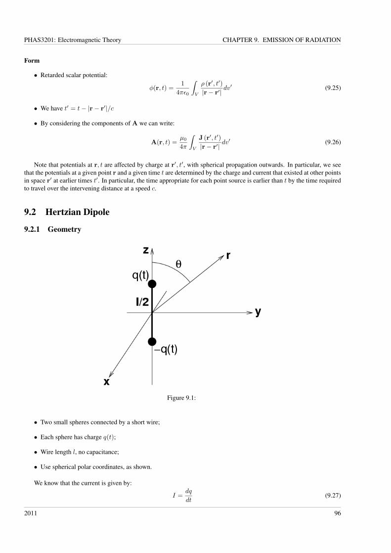
PHAS3201: Electromagnetic Theory CHAPTER 9. EMISSION OF RADIATION
Form
• Retarded scalar potential:
φ(r, t) =1
4πε0
∫V
ρ (r′, t′)
|r− r′|dv′ (9.25)
• We have t′ = t− |r− r′|/c
• By considering the components of A we can write:
A(r, t) =µ0
4π
∫V
J (r′, t′)
|r− r′|dv′ (9.26)
Note that potentials at r, t are affected by charge at r′, t′, with spherical propagation outwards. In particular, we seethat the potentials at a given point r and a given time t are determined by the charge and current that existed at other pointsin space r′ at earlier times t′. In particular, the time appropriate for each point source is earlier than t by the time requiredto travel over the intervening distance at a speed c.
9.2 Hertzian Dipole
9.2.1 Geometry
Figure 9.1:
• Two small spheres connected by a short wire;
• Each sphere has charge q(t);
• Wire length l, no capacitance;
• Use spherical polar coordinates, as shown.
We know that the current is given by:
I =dq
dt(9.27)
2011 96
PHAS3201: Electromagnetic Theory CHAPTER 9. EMISSION OF RADIATION
Now we can use the results from the previous section to write the vector potential:
Az(r, t) =µ0
4π
∫ l/2
−l/2
I(z′, t−
∣∣∣r− z′k∣∣∣ /c) dz′∣∣∣r− z′k∣∣∣ (9.28)
Jdv → Idl′ → Idz′ (9.29)
where the second set of equations follow from symmetry, and z′ lies on the wire. We can write:∣∣∣r− z′k∣∣∣ =
√(r − z′ cos θ)
2+ (z′ sin θ)
2 (9.30)
=(r2 − 2rz′ cos θ + z′ 2
) 12 (9.31)
= r
(1− 2
z′
rcos θ +
z′ 2
r2
) 12
(9.32)
' r − z′ cos θ, r >> z′ (9.33)
If we’re far away, then∣∣∣r− z′k∣∣∣ ≈ r. That takes care of the denominator; what about z′ cos θ/c ?
z′ cos θ ≤ l
2, (9.34)
by geometry. Now, if l2 << Tc for some period T , then l
2 << λ; this is the same as saying that we have a small dipole(in this case, relative to the wavelength). This enables us to write:
Az(r, t) ' µ0
4π
∫ l/2
−l/2
I (z′, t− r/c)r
dz′ (9.35)
=µ0
4π
(I(t− r/c)
r
)∫ l/2
−l/2dz′ (9.36)
=µ0l
4π
(I(t− r/c)
r
), (9.37)
as I is independent of z′. We can use the Lorentz condition, Eq. (9.12), to get the time variation of the scalar potential:
∇ ·A + ε0µ0∂φ
∂t= 0 (9.38)
⇒ ∂φ
∂t= − l
4πε0
∂
∂z
[1
rI(t− r
c
)](9.39)
There are various small results that we need:
r =√x2 + y2 + z2 (9.40)
∂r
∂z=
z
r(9.41)
∂
∂z
(1
r
)= − z
r3(9.42)
∂
∂t
(t− r
c
)= 1 (9.43)
Using these, we can rewrite Eq. (9.39) as:
∂φ
∂t= − l
4πε0
[− z
r3I(t− r
c
)− z
cr2
∂I(t− r/c)∂(t− r/c)
](9.44)
Finally we integrate with respect to time, remembering that, basically,∫Idt = q.
2011 97
PHAS3201: Electromagnetic Theory CHAPTER 9. EMISSION OF RADIATION
9.2.2 Potentials• The vector potential:
Az(r, t) =µ0l
4π
(I(t− r/c)
r
)(9.45)
• The scalar potential:
φ(r, t) =l
4πε0
z
r2
(q(t− r/c)
r+I(t− r/c)
c
)(9.46)
• Choose:q(t− r/c) = q0 cosω(t− r/c) (9.47)
This gives us the current:
I = −ωq0 sinω(t− r/c) (9.48)= I0 sinω(t− r/c) (9.49)
Then we can write for the vector potential in spherical polar coordinates (just reworking Eq. (9.45) again, taking thecomponents in the r and θ directions):
Ar =µ0
4π
I0l
rcos θ sinω(t− r/c) (9.50)
Aθ =µ0
4π
I0l
rsin θ sinω(t− r/c) (9.51)
Aφ = 0 (9.52)
If we use the standard formula for curl in spherical polar coordinates, we can calculate the magnetic field:
Br = 0 (9.53)Bθ = 0 (9.54)
Bφ =1
r
∂
∂r(rAθ)−
1
r
∂Ar∂θ
(9.55)
=µ0
4π
I0l
rsin θ
(ω
ccosω(t− r/c) +
1
rsinω(t− r/c)
)(9.56)
≈ µ0
4π
I0l
rsin θ
(ωc
cosω(t− r/c))
in the radiation zone, where r � c
ω, or r � λ. (9.57)
We get the electric field using:
E = −∇ϕ− ∂A
∂t(9.58)
Er = −∂φ∂r− ∂Ar
∂t= 0 (9.59)
Eθ = −1
r
∂φ
∂θ− ∂Aθ
∂t=lI0 sin θ
4πε0
ω cosω(t− r/c)rc2
(9.60)
Eφ = − 1
r sin θ
∂ϕ
∂φ− ∂Aφ
∂t= 0, (9.61)
where we have neglected terms in 1/r2 or higher.For reference, remember that I0 = −q0ω and p0 = q0l.
Important Points
• These do not depend on φ
• E and B are perpendicular
• The power is radially outwards, as E×B⇒ θ × φ = r
2011 98
PHAS3201: Electromagnetic Theory CHAPTER 9. EMISSION OF RADIATION
• The average power is:
P =l2ω2
6πε0c3I20
2(9.62)
• The radial components of E and B are zero
The radiated power is simply given by the surface integral of the Poynting vector.
W =
∮S
N · nda (9.63)
=1
µ0
∫ 2π
0
∫ π
0
BφEθr2 sin θdθdφ (9.64)
=ω2I2
0 l2
16π2ε0c3
∫ 2π
0
dφ
∫ π
0
sin3 θdθ cos2 (ω (t− r/c)) (9.65)
=ω2I2
0 l2
6πε0c3cos2 (ω (t− r/c)) (9.66)
When we average the cos2 term we recover the formula for average power above.
2011 99
PHAS3201: Electromagnetic Theory CHAPTER 9. EMISSION OF RADIATION
2011 100
PHAS3201: Electromagnetic Theory CHAPTER 10. RELATIVISTIC TRANSFORMATIONS
Chapter 10
Relativistic Transformations
We finish the course with a look at how the electric and magnetic fields are affected by transformations between differentinertial reference frames. This takes us into the realm of special relativity, and allows us both to see how the fields areintimately connected, and to derive Maxwell’s equations in a new and elegant way.
Classical electrodynamics is already consistent with special relativity. Maxwell’s equations and the Lorentz force lawcan be applied in any inertial system, although what one observer interprets as electrical another may regard as magneticwith the actual particle motions identical. This section will hopefully give you a deeper appreciation of the structure ofelectrodynamics – laws that had seemed arbitrary and unrelated before take on a certain coherence and inevitability whenlooked at from the point of view of relativity.
10.1 Introduction
10.1.1 Basic Principles• Laws of physics are the same in all inertial reference frames;
• Speed of light in vacuum is the same in all reference frames;
• It is also independent of the motion of the emitting body;
• Inertial reference frame is not accelerating.
Start with sound: if we measure its speed relative to stationary air, then we get something around 330 metres persecond (note that this will depend on temperature and pressure). If we measure it in a moving inertial reference frame wecan get a different answer if the air is no longer stationary.
Any wave (or wave-like disturbance) which does not require a medium to propagate must travel at the same speed inall reference frames (otherwise we could do an experiment to differentiate between them). This was the basis of Einstein’sprinciple of relativity.
What about coordinate systems? We must specify a set of axes associated with an inertial reference frame (notice thatif we were being exact, we’d refer to a rigid inertial reference frame). We’ll call our frame S, and associate the distancesalong axes x, y and z with the axes. In order to specify events, we must also specify a time, t. We will use the notationS(x, y, z, t) to specify a reference frame and the coordinates in that frame.
10.1.2 Coordinate transforms• Two inertial frames: S(x, y, z, t) and S′(x′, y′, z′, t′)
• S′ moves with velocity v in the x direction of S
• At t = t′ = 0, x = x′ = 0
• An event P at (x, y, z, t) in S has coordinates (x′, y′, z′, t′) in S′
• The origins in S and S′ coincide at t = t′ = 0
2011 101
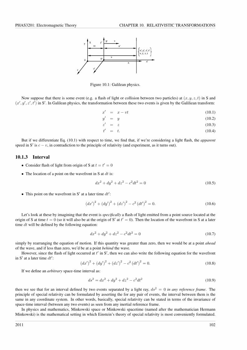
PHAS3201: Electromagnetic Theory CHAPTER 10. RELATIVISTIC TRANSFORMATIONS
Figure 10.1: Galilean physics.
Now suppose that there is some event (e.g. a flash of light or collision between two particles) at (x, y, z, t) in S and(x′, y′, z′, t′) in S′. In Galilean physics, the transformation between these two events is given by the Galiliean transform:
x′ = x− vt (10.1)y′ = y (10.2)z′ = z (10.3)t′ = t. (10.4)
But if we differentiate Eq. (10.1) with respect to time, we find that, if we’re considering a light flash, the apparentspeed in S′ is c− v, in contradiction to the principle of relativity (and experiment, as it turns out).
10.1.3 Interval• Consider flash of light from origin of S at t = t′ = 0
• The location of a point on the wavefront in S at dt is:
dx2 + dy2 + dz2 − c2dt2 = 0 (10.5)
• This point on the wavefront in S′ at a later time dt′:
(dx′)2
+ (dy′)2
+ (dz′)2 − c2 (dt′)
2= 0. (10.6)
Let’s look at these by imagining that the event is specifically a flash of light emitted from a point source located at theorigin of S at time t = 0 (so it will also be at the origin of S′ at t′ = 0). Then the location of the wavefront in S at a latertime dt will be defined by the following equation:
dx2 + dy2 + dz2 − c2dt2 = 0 (10.7)
simply by rearranging the equation of motion. If this quantity was greater than zero, then we would be at a point aheadof the wave, and if less than zero, we’d be at a point behind the wave.
However, since the flash of light occurred at t′ in S′, then we can also write the following equation for the wavefrontin S′ at a later time dt′:
(dx′)2
+ (dy′)2
+ (dz′)2 − c2 (dt′)
2= 0. (10.8)
If we define an arbitrary space-time interval as:
ds2 = dx2 + dy2 + dz2 − c2dt2 (10.9)
then we see that for an interval defined by two events separated by a light ray, ds2 = 0 in any reference frame. Theprinciple of special relativity can be formulated by asserting the for any pair of events, the interval between them is thesame in any coordinate system. In other words, basically, special relativity can be stated in terms of the invariance ofspace-time interval (between any two events) as seen from any inertial reference frame.
In physics and mathematics, Minkowski space or Minkowski spacetime (named after the mathematician HermannMinkowski) is the mathematical setting in which Einstein’s theory of special relativity is most conveniently formulated.
2011 102
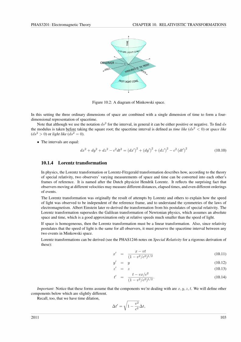
PHAS3201: Electromagnetic Theory CHAPTER 10. RELATIVISTIC TRANSFORMATIONS
Figure 10.2: A diagram of Minkowski space.
In this setting the three ordinary dimensions of space are combined with a single dimension of time to form a four-dimensional representation of spacetime.
Note that although we use the notation ds2 for the interval, in general it can be either positive or negative. To find dsthe modulus is taken before taking the square root; the spacetime interval is defined as time like (ds2 < 0) or space like(ds2 > 0) or light like (ds2 = 0).
• The intervals are equal:
dx2 + dy2 + dz2 − c2dt2 = (dx′)2
+ (dy′)2
+ (dz′)2 − c2 (dt′)
2 (10.10)
10.1.4 Lorentz transformation
In physics, the Lorentz transformation or Lorentz-Fitzgerald transformation describes how, according to the theoryof special relativity, two observers’ varying measurements of space and time can be converted into each other’sframes of reference. It is named after the Dutch physicist Hendrik Lorentz. It reflects the surprising fact thatobservers moving at different velocities may measure different distances, elapsed times, and even different orderingsof events.
The Lorentz transformation was originally the result of attempts by Lorentz and others to explain how the speedof light was observed to be independent of the reference frame, and to understand the symmetries of the laws ofelectromagnetism. Albert Einstein later re-derived the transformation from his postulates of special relativity. TheLorentz transformation supersedes the Galilean transformation of Newtonian physics, which assumes an absolutespace and time, which is a good approximation only at relative speeds much smaller than the speed of light.
If space is homogeneous, then the Lorentz transformation must be a linear transformation. Also, since relativitypostulates that the speed of light is the same for all observers, it must preserve the spacetime interval between anytwo events in Minkowski space.
Lorentz transformations can be derived (see the PHAS1246 notes on Special Relativity for a rigorous derivation ofthese):
x′ =x− vt
(1− v2/c2)1/2(10.11)
y′ = y (10.12)z′ = z (10.13)
t′ =t− vx/c2
(1− v2/c2)1/2. (10.14)
Important: Notice that these forms assume that the components we’re dealing with are x, y, z, t. We will define othercomponents below which are slightly different.
Recall, too, that we have time dilation,
∆t′ =
√1− v2
c2∆t,
2011 103
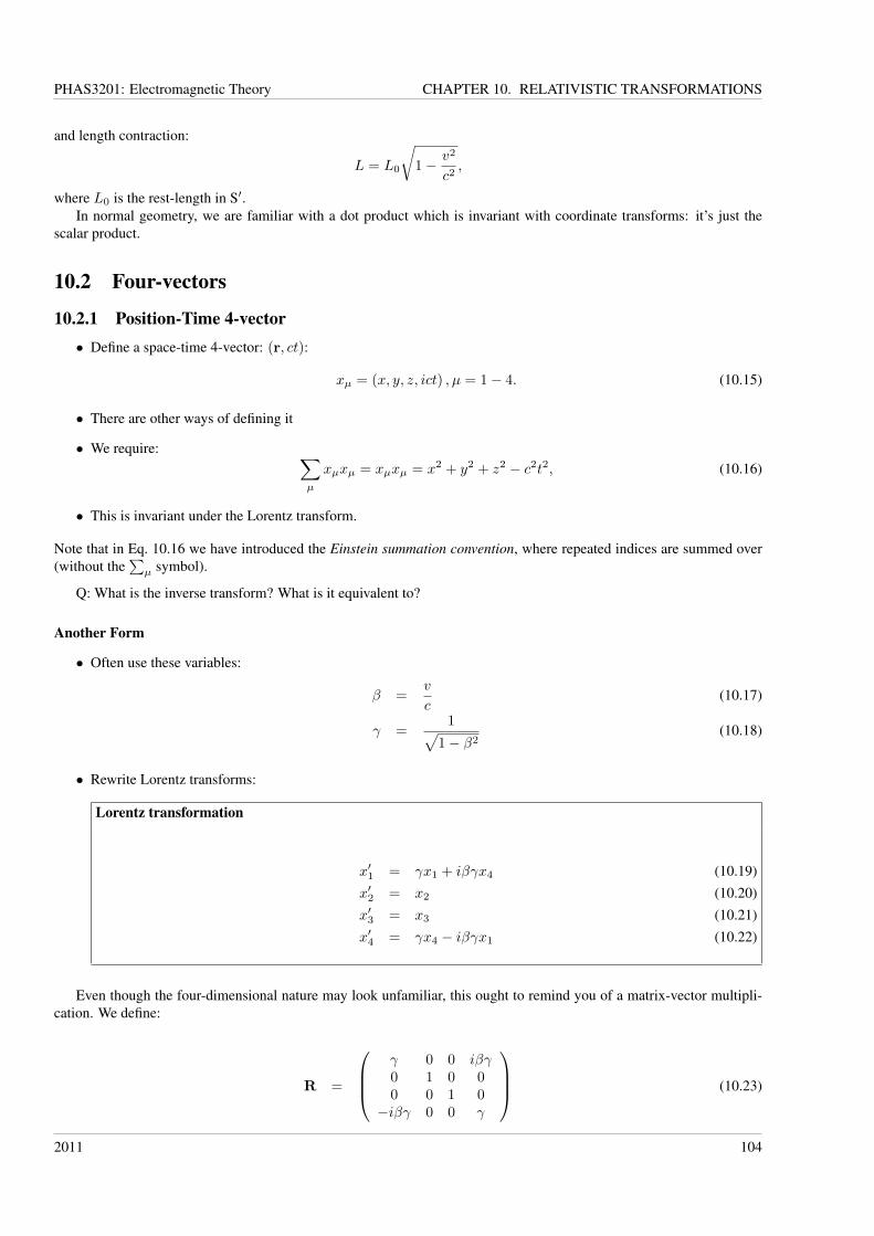
PHAS3201: Electromagnetic Theory CHAPTER 10. RELATIVISTIC TRANSFORMATIONS
and length contraction:
L = L0
√1− v2
c2,
where L0 is the rest-length in S′.In normal geometry, we are familiar with a dot product which is invariant with coordinate transforms: it’s just the
scalar product.
10.2 Four-vectors
10.2.1 Position-Time 4-vector• Define a space-time 4-vector: (r, ct):
xµ = (x, y, z, ict) , µ = 1− 4. (10.15)
• There are other ways of defining it
• We require: ∑µ
xµxµ = xµxµ = x2 + y2 + z2 − c2t2, (10.16)
• This is invariant under the Lorentz transform.
Note that in Eq. 10.16 we have introduced the Einstein summation convention, where repeated indices are summed over(without the
∑µ symbol).
Q: What is the inverse transform? What is it equivalent to?
Another Form
• Often use these variables:
β =v
c(10.17)
γ =1√
1− β2(10.18)
• Rewrite Lorentz transforms:
Lorentz transformation
x′1 = γx1 + iβγx4 (10.19)x′2 = x2 (10.20)x′3 = x3 (10.21)x′4 = γx4 − iβγx1 (10.22)
Even though the four-dimensional nature may look unfamiliar, this ought to remind you of a matrix-vector multipli-cation. We define:
R =
γ 0 0 iβγ0 1 0 00 0 1 0−iβγ 0 0 γ
(10.23)
2011 104
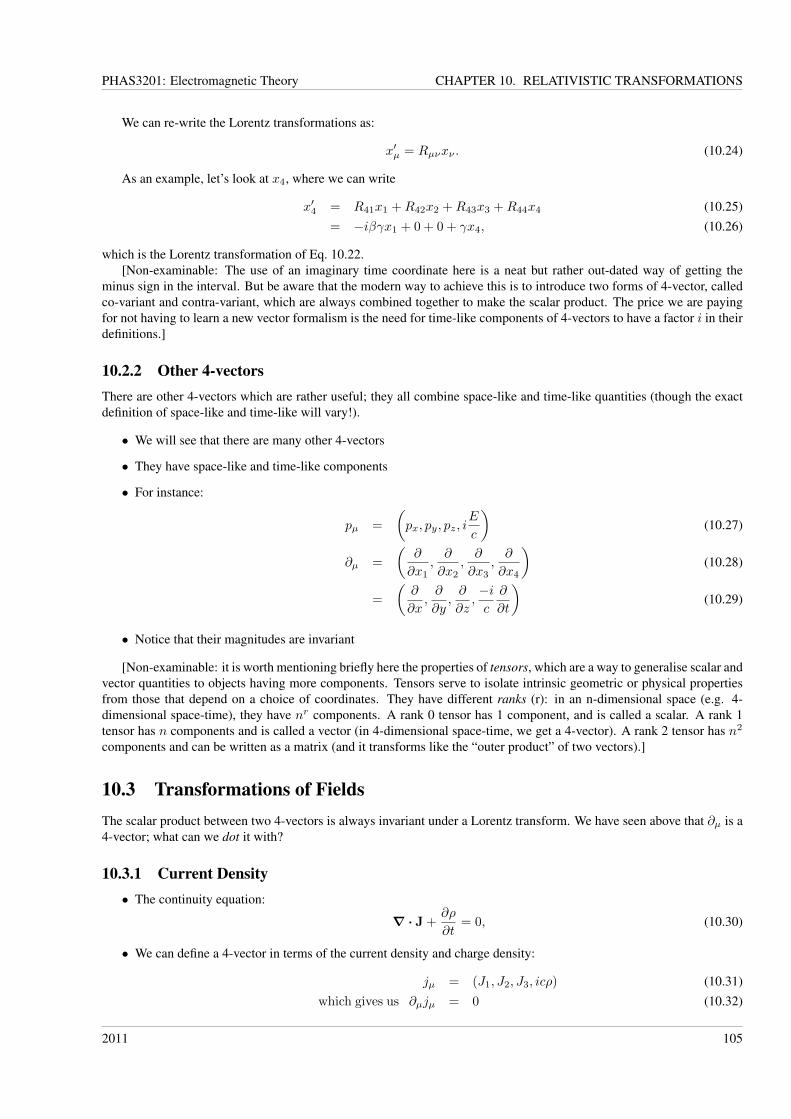
PHAS3201: Electromagnetic Theory CHAPTER 10. RELATIVISTIC TRANSFORMATIONS
We can re-write the Lorentz transformations as:
x′µ = Rµνxν . (10.24)
As an example, let’s look at x4, where we can write
x′4 = R41x1 +R42x2 +R43x3 +R44x4 (10.25)= −iβγx1 + 0 + 0 + γx4, (10.26)
which is the Lorentz transformation of Eq. 10.22.[Non-examinable: The use of an imaginary time coordinate here is a neat but rather out-dated way of getting the
minus sign in the interval. But be aware that the modern way to achieve this is to introduce two forms of 4-vector, calledco-variant and contra-variant, which are always combined together to make the scalar product. The price we are payingfor not having to learn a new vector formalism is the need for time-like components of 4-vectors to have a factor i in theirdefinitions.]
10.2.2 Other 4-vectorsThere are other 4-vectors which are rather useful; they all combine space-like and time-like quantities (though the exactdefinition of space-like and time-like will vary!).
• We will see that there are many other 4-vectors
• They have space-like and time-like components
• For instance:
pµ =
(px, py, pz, i
E
c
)(10.27)
∂µ =
(∂
∂x1,∂
∂x2,∂
∂x3,∂
∂x4
)(10.28)
=
(∂
∂x,∂
∂y,∂
∂z,−ic
∂
∂t
)(10.29)
• Notice that their magnitudes are invariant
[Non-examinable: it is worth mentioning briefly here the properties of tensors, which are a way to generalise scalar andvector quantities to objects having more components. Tensors serve to isolate intrinsic geometric or physical propertiesfrom those that depend on a choice of coordinates. They have different ranks (r): in an n-dimensional space (e.g. 4-dimensional space-time), they have nr components. A rank 0 tensor has 1 component, and is called a scalar. A rank 1tensor has n components and is called a vector (in 4-dimensional space-time, we get a 4-vector). A rank 2 tensor has n2
components and can be written as a matrix (and it transforms like the “outer product” of two vectors).]
10.3 Transformations of FieldsThe scalar product between two 4-vectors is always invariant under a Lorentz transform. We have seen above that ∂µ is a4-vector; what can we dot it with?
10.3.1 Current Density• The continuity equation:
∇ · J +∂ρ
∂t= 0, (10.30)
• We can define a 4-vector in terms of the current density and charge density:
jµ = (J1, J2, J3, icρ) (10.31)which gives us ∂µjµ = 0 (10.32)
2011 105
PHAS3201: Electromagnetic Theory CHAPTER 10. RELATIVISTIC TRANSFORMATIONS
Since the differential operator ∂µ transforms as a 4-vector and the RHS is a scalar and this equation should be truein any inertial frame, we must have that jµ also transforms as a 4-vector. The 4-vector nature of jµ can also be shownby considering a distribution of moving point charges and finding how the current and charge densities vary in differentframes.
10.3.2 PotentialsWe can now consider the electromagnetic potentials, which are related to the different components of the current density4-vector:
∇2A− 1
c2∂2A
∂t2= −µ0J (10.33)
∇2φ− 1
c2∂2φ
∂t2= − 1
ε0ρ (10.34)
To put these in Lorentz invariant form, we define the 4-dimensional Laplacian operator (or d’Alembertian) as the dotproduct between the ∂µ 4-vector and itself.
• Define the 4D Laplacian (like∇2)
∂µ∂µ = 2 (10.35)
Now define a 4-vector in terms of the vector and scalar potentials:
aµ =
(A1, A2, A3,
iφ
c
)(10.36)
⇒ 2aµ = −µ0jµ (10.37)
• We can write the Lorentz condition as:∂µaµ = 0 (10.38)
As 2 is a scalar, and the right-hand side of Eq. (10.36) transforms as a 4-vector then aµ must also transform as a4-vector if the equation is to apply in all references frames.
This scalar product in Eq. (10.38) is manifestly invariant under Lorentz transforms, so that if we fulfil the Lorentzcondition in one reference frame, we will fulfil it in all frames. It can also be shown (though we don’t have time) that thesolutions for the retarded potentials derived in Section 10 are parts of a 4-vector which transforms in the usual way.
10.3.3 FieldsEquations (10.36) and (10.38) correspond to Maxwell’s equations written in covariant form in terms of potentials. Nowwe move on to the electric and magnetic fields, which we will find that we can write in terms of a single tensor. How willwe arrive at this point?
Consider the definitions of the fields in terms of the potentials:
B = ∇×A (10.39)
E = −∇φ− ∂A
∂t(10.40)
• Write the components of fields in terms of potentials
B1 =∂a3
∂x2− ∂a2
∂x3(10.41)
− icE1 =
∂a4
∂x1− ∂a1
∂x4(10.42)
• Together they resemble the parts of a kind of 4-D curl
2011 106
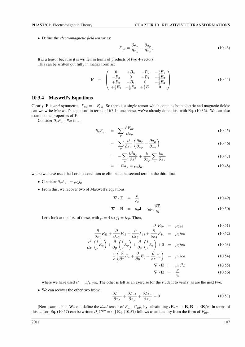
PHAS3201: Electromagnetic Theory CHAPTER 10. RELATIVISTIC TRANSFORMATIONS
• Define the electromagnetic field tensor as:
Fµν =∂aν∂xµ
− ∂aµ∂xν
, (10.43)
It is a tensor because it is written in terms of products of two 4-vectors.This can be written out fully in matrix form as:
F =
0 +B3 −B2 − i
cE1
−B3 0 +B1 − icE2
+B2 −B1 0 − icE3
+ icE1 + i
cE2 + icE3 0
(10.44)
10.3.4 Maxwell’s EquationsClearly, F is anti-symmetric: Fµν = −Fνµ. So there is a single tensor which contains both electric and magnetic fields:can we write Maxwell’s equations in terms of it? In one sense, we’ve already done this, with Eq. (10.36). We can alsoexamine the properties of F.
Consider ∂νFµν . We find:
∂νFµν =∑ν
∂Fµν∂xν
(10.45)
=∑ν
∂
∂xν
(∂aν∂xµ
− ∂aµ∂xν
)(10.46)
= −∑ν
∂2aµ∂x2
ν
+∂
∂xµ
∑ν
∂aν∂xν
(10.47)
= −2aµ = µ0jµ, (10.48)
where we have used the Lorentz condition to eliminate the second term in the third line.
• Consider ∂νFµν = µ0jµ
• From this, we recover two of Maxwell’s equations:
∇ ·E =ρ
ε0(10.49)
∇×B = µ0J + ε0µ0∂E
∂t(10.50)
Let’s look at the first of these, with µ = 4 so j4 = icρ. Then,
∂νF4ν = µ0j4 (10.51)∂
∂x1F41 +
∂
∂x2F42 +
∂
∂x3F43 +
∂
∂x4F44 = µ0icρ (10.52)
∂
∂x
(i
cEx
)+
∂
∂y
(i
cEy
)+
∂
∂z
(i
cEz
)+ 0 = µ0icρ (10.53)
i
c
(∂
∂xEx +
∂
∂yEy +
∂
∂zEz
)= µ0icρ (10.54)
∇ ·E = µ0c2ρ (10.55)
∇ ·E =ρ
ε0(10.56)
where we have used c2 = 1/µ0ε0. The other is left as an exercise for the student to verify, as are the next two.
• We can recover the other two from:∂Fµν∂xλ
+∂Fνλ∂xµ
+∂Fλµ∂xν
= 0 (10.57)
[Non-examinable: We can define the dual tensor of Fµν , Gµν , by substituting iE/c → B,B → iE/c. In terms ofthis tensor, Eq. (10.57) can be written ∂µGµν = 0.] Eq. (10.57) follows as an identity from the form of Fµν .
2011 107
PHAS3201: Electromagnetic Theory CHAPTER 10. RELATIVISTIC TRANSFORMATIONS
Important Points
• The electric and magnetic fields can be written as a single tensor
• Maxwell’s equations can be written rather simply in terms of this tensor
• They are manifestly invariant under Lorentz co-ordinate transforms
• Transform F between frames using R:F′ = RFRT (10.58)
In terms of components, we can write:
F ′µν =∑α
∑β
RµαFαβRνβ . (10.59)
Then, for instance, we can find transformations of the E and B fields, such as:
B′3 = F ′12 =
4∑α=1
4∑β=1
R1αFαβR2β .
10.3.5 TransformationsIt is also possible to get the transformation by considering the fields in terms of the potentials and differentials, andtransforming them separately. This requires a little algebra.
• In any case. we find the transformations of E and B between frames:
Field transformations
E′‖ = E‖ (10.60)
E′⊥ = γE⊥ + γv ×B (10.61)B′‖ = B‖ (10.62)
B′⊥ = γB⊥ −1
c2γv ×E, (10.63)
• The two frames move with velocity v relative to each other
• the directions are parallel and perpendicular to the velocity.
Notice which components are left unchanged (by comparison to lengths) and how we can do a certain amount rathereasily. This transformation mixes the fields.
If we start with a set of potentials due to a stationary charge in frame S′, then we can write:
A′ = 0 (10.64)
φ′ =e
4πε0r′(10.65)
Now we transform to the frame S:
A1 = γ
(A′1 − i
u
c· iφ′
c
)=
γue
4πε0c2r′(10.66)
A2 = A′2 = 0 (10.67)A3 = A′3 = 0 (10.68)iφ
c= γ
(iφ′
c+u
cA′1
)=i
c
γe
4πε0r′(10.69)
2011 108
PHAS3201: Electromagnetic Theory CHAPTER 10. RELATIVISTIC TRANSFORMATIONS
Notice how the movement of the charge due to the change in reference frame now gives a non-zero vector potential.The final form of the transformation is not quite as simple as it looks because the radial component r′ needs to betransformed as well.
[Non-examinable: The rigorous way to demonstrate the Lorentz invariance of electromagnetic theory is to begin withthe definition of the field quantity Fµν and write the Lorentz force law for a moving charged particle in terms of this.Then the requirement that the motion of this particle should transform according to the rules of Lorentzian mechanics fora particle with constant rest mass leads to the assertion that Fµν indeed transforms like a tensor. It can be shown thatthe fact that it is antisymmetric means that it can be written as the 4-curl of a 4-vector which then turns out to be the4-potential aµ. By this route the law of conservation of charge can be shown to be a consequence of Lorentz invariance.]
2011 109
![Electromagnetic Field Theory [eBook]](https://static.fdocuments.us/doc/165x107/54782f0fb4af9f63108b4b45/electromagnetic-field-theory-ebook.jpg)