PFE Simulation Methodology

Copyright © 2006, SAS Institute Inc. All rights reserved.

PFE Simulation MethodologyDominic J PazzulaSr. Consultant – RiskAdvisory


About RiskAdvisory

RiskAdvisory (A Division of SAS) RiskAdvisory is a leading provider of integrated risk solutions to energy companies operating in today's volatile energy commodity markets. Founded in 1995 by accomplished energy risk professionals, the company has provided risk software solutions, management consulting and educational services to over 220 clients in the global energy sector.

Headquartered in Calgary, Canada, RiskAdvisory produces software solutions that are used by a growing number of well-known energy companies. RiskAdvisory was acquired by business intelligence software leader SAS in 2003.


What is PFE?

• Exposure – The amount of money I would lose if a counterparty defaulted.

• Future Exposure – Exposure at a future point in time.

• Potential Future Exposure – Maximum exposure under normal market conditions for a future point in time.


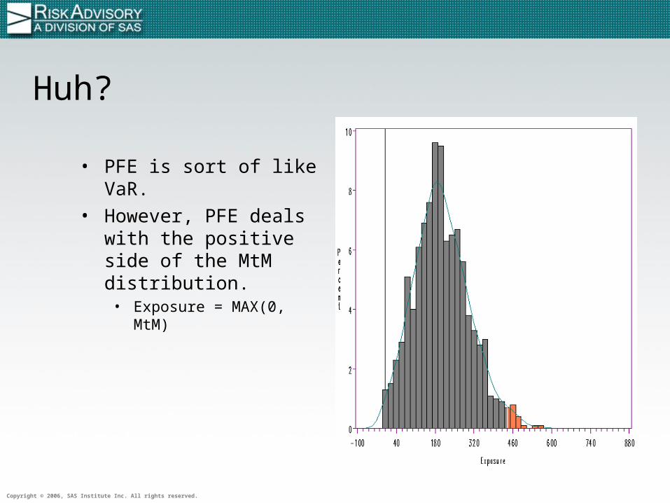
Huh?

• PFE is sort of like VaR.• However, PFE deals with

the positive side of the MtM distribution.

• Exposure = MAX(0, MtM)


Holding Period

• Unlike VaR, PFE usually looks at long holding periods.– VaR is usually concerned with short term fluctuations.

• Default risk is usually negligible in the short term.


PFE Through Time

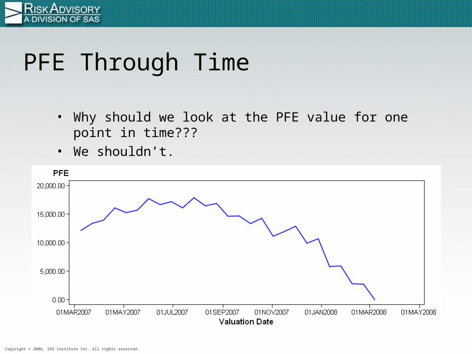
• Why should we look at the PFE value for one point in time???

• We shouldn’t.


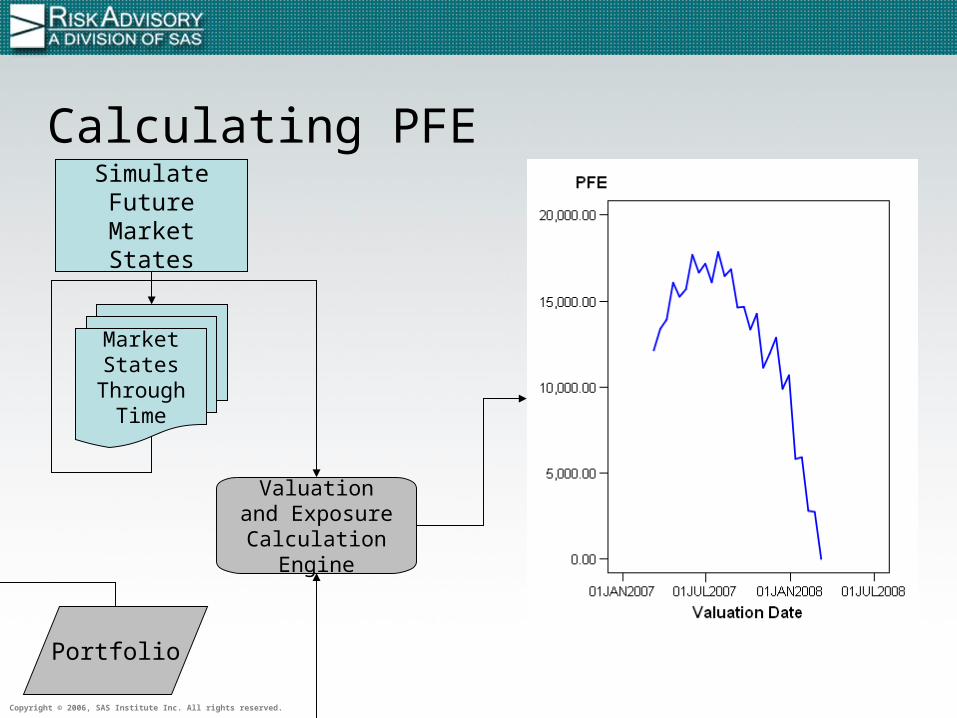
Calculating PFESimulate Future Market States

Market States

Through Time

Portfolio

Valuation and Exposure

Calculation Engine


Issues with Long Dated Simulations

• Shape of the volatility forward curve• Non-normality of price distributions• Seasonality of both prices and volatility• Shifting Correlations


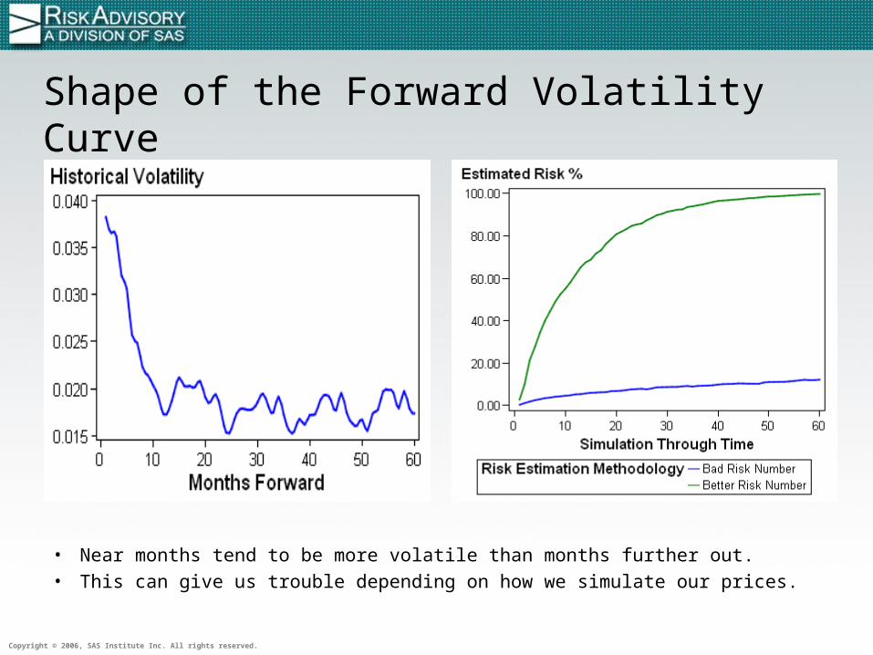
Shape of the Forward Volatility Curve

• Near months tend to be more volatile than months further out.

• This can give us trouble depending on how we simulate our prices.


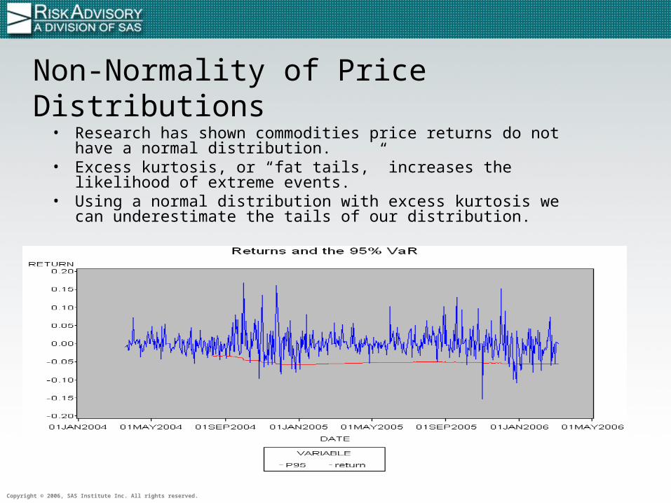
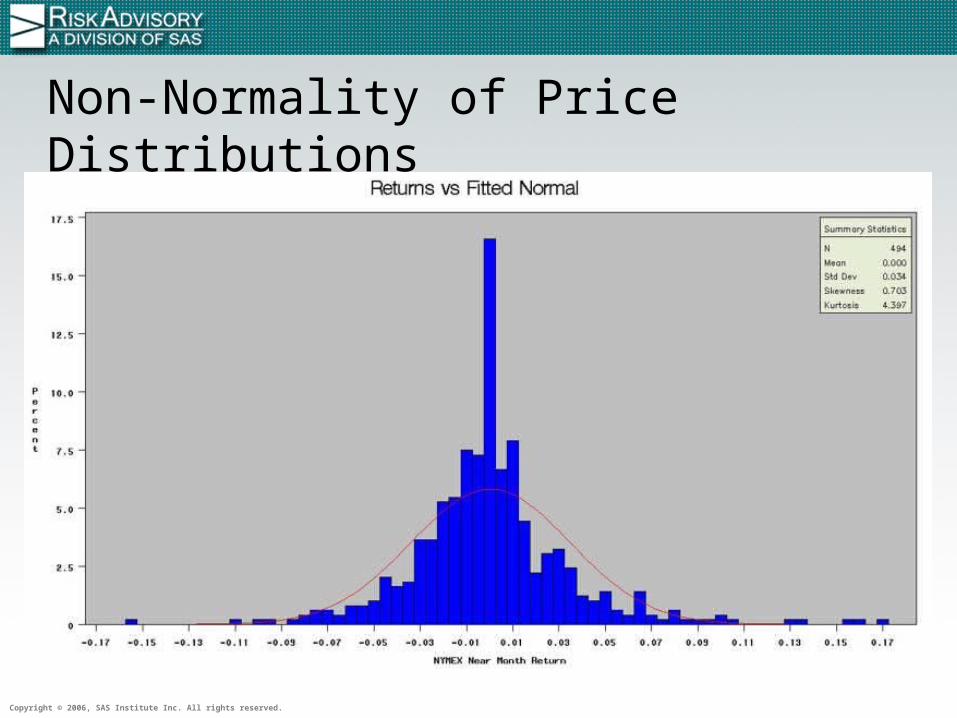
Non-Normality of Price Distributions• Research has shown commodities price returns do not have a

normal distribution.• Excess kurtosis, or “fat tails,” increases the likelihood of extreme

events.• Using a normal distribution with excess kurtosis we can

underestimate the tails of our distribution.


Non-Normality of Price Distributions


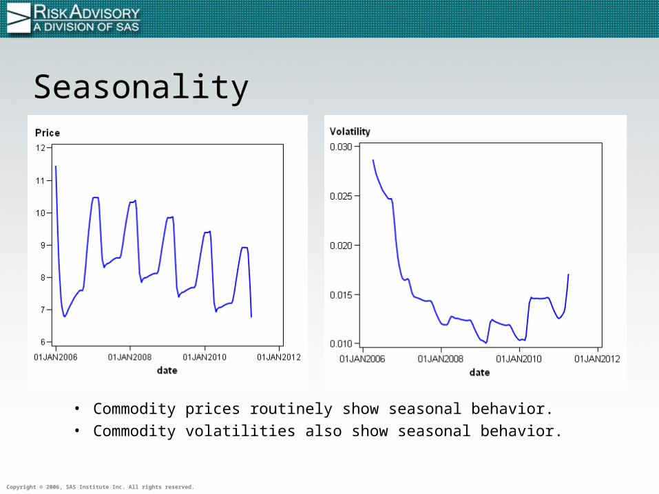
Seasonality

• Commodity prices routinely show seasonal behavior.• Commodity volatilities also show seasonal behavior.


Shifting Correlations

• Correlations are not constant, but most models assume they are.

• As correlations approach 1(-1), aR numbers for an entire portfolio will increase (decrease).

• Nirvana would be a model that dynamically simulates correlations as well as prices.

• Data is an issue.


Three Simulation Methodologies

• Modified Covariance Simulation• Model Based Simulation• PCA Simulation of Forward Curves


Modified Covariance Simulation – Model Definition

• Price returns are assumed to be normally distributed.

• Variance and Correlations are calculated based on static prices.

• Variances are updated using market observed implied volatilities.


Modified Covariance Simulation – Pros

• Volatility curve issues are handled by using the implied volatilities.

• Simple, easy to implement, and can be explained to management and auditors.


Modified Covariance Simulation – Cons

• The model relies on normality assumptions that we know do not hold.

• Data for implied volatilities may be stale or non-existent.


Model Based Simulation – Model Definition

• Static prices are modeled using econometric techniques.

• SAS Whitepaper available at: http://

www.riskadvisory.com/pdfs/sasriskdimensionsriskfactor.pdf


Model Based Simulation – Pros

• No normality assumptions.• Modeler has full control over how the prices are

simulated.• Can closely match simulated values to observed

distributions.


Model Based Simulation – Cons

• The modeler’s job is a big one.• What worked last month may not work this

month.• Automated fitting processes have to be

concerned with model convergence.


PCA Simulation of Forward Curves – Model Definition

• Forward curve is simulated relative prices and volatilities.

• Principal Component Analysis (PCA) is used to reduce the dimensionality of the simulation.

• PCA components are modeled using a covariance simulation.


PCA Simulation of Forward Curves – Pros

• Forward volatility curve is taken into account.• Simulated variables are minimized.


PCA Simulation of Forward Curves – Cons

• PCA still assumes underlying normality of points along the forward curve.

• Business logic must be implemented to insure the correct volatilities and prices are aligned for each step in the simulation.


Final Thoughts

• PFE models need to capture realistic market movements.

• PFE models have to be explainable.• PFE models have to be implemented and

maintained.• PFE modeling is a balancing act between these

three issues.


Questions?

Dominic Pazzula – [email protected]

PFE Simulation Methodology

Documents

Transcript of PFE Simulation Methodology