PETROPHYSICAL EVALUATION OF THE ALBIAN AGE GAS … · Petrophysical evaluation of the Albian age...

PETROPHYSICAL EVALUATION OF THE ALBIAN AGE GAS BEARING SANDSTONE

RESERVOIRS OF THE O-M FIELD, ORANGE BASIN, SOUTH AFRICA

By

OPUWARI, MIMONITU

A thesis Submitted in Partial fulfilment of the requirement for the degree of Philosophae Doctor

(PhD) in the Faculty of Science, Earth Sciences Department

University of the Western Cape, Bellville, South Africa

Supervisor: Professor Paul Carey

Co-supervisor: Escordia De Poquioma

May, 2010.

i

ABSTRACT

Petrophysical Evaluation of the Albian Age Gas Bearing Sandstone Reservoirs of the O-M field,

Orange Basin, South Africa

Opuwari, Mimonitu

Petrophysical evaluation of the Albian age gas bearing sandstone reservoirs of the O-M field,

Offshore South Africa has been performed. The main goal of the thesis is to evaluate the

reservoir potentials of the field through the integration and comparison of results from core

analysis, production data and petrography studies for the evaluation and correction of key

petrophysical parameters from wireline logs which could be used to generate an effective

reservoir model. A total of ten wells were evaluated and twenty eight sandstone reservoirs were

encountered of which twenty four are gas bearing and four are wet within the Albian age depth

interval of 2800m to 3500m. Six lithofacies (A1, A2, A3, A4, A5 and A6) were grouped

according to textural and structural features and grain size from the key wells (OP1, OP2 and

OP3). Facies A6 was identified as non reservoir rock in terms of reservoir rock quality and facies

A1 and A2 were regarded as the best reservoir rock quality. This study identifies the different

rock types that comprise reservoir and non reservoirs. Porosity and permeability are the key

parameters for identifying the rock types and reservoir characterization. Pore throat radius was

estimated from conventional core porosity and permeability with application of the Winland’s

method for assessment of reservoir rock quality on the bases of pore throat radius. Results from

the Winland’s method present five Petrofacies (Mega porous, Macro porous, Meso porous,

Micro porous and Nanno porous). The best Petrofacies was mega porous rock type which

corresponds to lithofacies A1 and A2. The nano porous rock type corresponds to lithofacies A6

and was subsequently classified as non reservoir rock. The volume of clay model from log was

taken from the gamma-ray model corrected by Steiber equations which was based on the level of

agreement between log data and the x-ray diffraction (XRD) clay data. The average volume of

clay determined ranged from 1 – 28 %. The field average grain density of 2.67 g/cc was

ii

determined from core data which is representative of the well formation, hence 2.67 g/cc was

used to estimate porosity from the density log. Reservoir rock properties are generally good with

reservoir average porosities between 10 – 22 %, an average permeability of approximately

60mD. The laterolog resistivity values have been invasion corrected to yield estimates of the true

formation resistivity. In general, resistivities of above 4.0 Ohm-m are productive reservoirs, an

average water resistivity of 0.1 Ohm-m was estimated. Log calculated water saturation models

were calibrated with capillary pressure and conventional core determined water saturations, and

the Simandoux shaly sand model best agree with capillary and conventional core water

saturations and was used to determine field water saturations. The reservoir average water

saturations range between 23 – 69 %. The study also revealed quartz as being the dominant

mineral in addition to abundant chlorite as the major clay mineral. The fine textured and

dispersed pore lining chlorite mineral affects the reservoir quality and may be the possible cause

of the low resistivity recorded in the area. The reservoirs evaluated in the field are characterized

as normally pressured with an average reservoir pressure of 4800 psi and temperature of 220 ºF.

An interpreted field aquifer gradient of 0.44 psi/ft (1.01 g/cc) and gas gradient of 0.09 psi/ft (0.2

g/cc) were obtained from repeat formation test measurements. A total of eight gas water contacts

were identified in six wells. For an interval to be regarded as having net pay potential, cut-off

values were used to distinguish between pay and non-pay intervals. For an interval to be

regarded as pay, it must have a porosity value of at least 10 %, volume of clay of less than 40 %,

and water saturation of not more than 65 %. A total of twenty four reservoir intervals meet the

cut-off criteria and was regarded as net pay intervals. The gross thickness of the reservoirs range

from 2.4m to 31.7m and net pay interval from 1.03m to 25.15m respectively. In summary, this

study contributes to scale transition issues in a complex gas bearing sandstone reservoirs and

serves as a basis for analysis of petrophysical properties in a multi-scale system.

iii

DECLARATION

I declare that Petrophysical Evaluation of the Albian Age Gas Bearing Sandstone Reservoirs

of the O-M field, Orange Basin, South Africa is my own work, that it has not been submitted

before for any degree or examination in any other university, and that all the sources I have used

or quoted have been indicated and acknowledged as complete references.

Opuwari, Mimonitu May 2010

Signed: ……………………………..

iv

ACKNOWLEDGEMENTS

I would like to give the Almighty God all the glory, honour and adoration for seeing me through

this great journey of overwhelming challenges. With His presence, it has really been an

interesting and fulfilling venture. A number of persons have contributed throughout the period of

this project and deserve credit for the completion of this project.

To my supervisors, Professor Paul Carey and Escordia de Poquioma (Mrs), I say a big thank you

for your untiring efforts and interest in this work. You introduced me to the world of

Petrophysics and ensured that I receive water, care and nourishment from time to time. Your

confidence in me was indeed a great inspiration. From time to time, you were ever willing to

attend to my “don’t knows”. The fruit of your support is evident, and I am indeed very grateful.

This research project was financially supported by the Petroleum oil and gas company of South

Africa (PETROSA) and I am deeply grateful for such an opportunity. The contributions of

Petroleum Agency of South Africa (PASA) and Forest Oil Exploration International for

providing data used in this thesis are highly acknowledged. I am also grateful to Schlumberger

Company and Senergy for providing the Interactive Petrophysics Software package used in the

modeling.

Mr Jeff Aldrich is gratefully acknowledged for his general support, motivation and the trust he

demonstrated especially at the early phase of this research work. Mr Andrew and Jody Frewin’s

contributions to the success of this work are appreciated. Thanks a lot.

The dean of Science, Professor Donker is deeply appreciated for his support at critical stages of

this work.

To the Department of Earth Sciences, University of the Western Cape, Bellville, South Africa,

the Head of the department, Prof. Charles Okujeni and all the members of staff, I say a big thank

you for the good and cordial working relationship I enjoyed during my studies. Fellow students

in the department, especially Solomon Adekola, Segun Adeyemi, Corlyne Barlie, Fadipe,

v

Wisemen, Yafeh, Funke Ojo, are appreciated for the professional and non- professional

conversations during this period. The secretary, Ms Washiela Davids is thanked for her support.

This study would not have been completely satisfying without the working relationship I had

with my colleagues and good brothers, including James Ayuk, Dr Richard Akinyeye, Anthony

Duah, Ebenezer Kingsley, Jerry Egwu, Joe Daniel, Greene Avor, Seth Udeme, Dr Patrick Ogidi,

Sunmi Iyela, Femi Adigun , and Victor Amadi. Your contributions are highly appreciated.

I wish to thank Rev Segun Adeleke, Professor and Mrs Meshack Ogunniye, Professor and Dr

Charles Ile, Professor George Amabeoku, Rev George Ogenetega, Pastor Akinyeye, Lanre

Fatoba, and members of Boston Cell group of Bellville Baptist Church for their prayers and

support. I am indeed very proud of you.

Mr Abdullah Jamoodian, Mandla N,Rasheed ,and Sbusiso all of PetroSA are appreciated for

their support. Also to be remembered is Mr Juan Carlos Porras of International rock Analysts for

the short course he presented on rock typing. Thank you.

I am particularly grateful to my parents, Mr and Mrs Ahams Opuwari for my education and

upbringing and my in-laws for their prayers and support. It is delightful to see you all alive as I

progress in life. All my other family members are equally gratefully acknowledged. Thanks for

the love and care.

Finally, my dear wife, Chinyerum and son David are thanked for showing an enormous patience

and understanding during this period of study. I could not have carried out this research without

her caring support. I really appreciate and love you dearly.

vi

DEDICATION

This project is dedicated to

The

ALMIGHTY GOD

for

His

Enabling Grace that was

Sufficient for me.

vii

TABLE OF CONTENTS

Page No

Abstract i

Declaration iii

Acknowledgements iv

Dedication v

Table of contents vii

List of Figures xvi

List of Tables xxiii

List of Appendices xxvi

SECTION ONE: BASIC CONCEPTS

Chapter One: Introduction 1

1.1 Background Information 1

1.2 Approach and outline of thesis 2

1.3 Geological Overview 5

1.4 Location of Study Area/ Well Location 7

1.5 Aims and Objectives 9

1.6 Research Methodology 9

Chapter Two: Wireline Logging 13

2.1 Introduction 13

2.2 The Nuclear Logs 14

2.2.1 Conventional Natural Gamma Ray (GR) 14

2.2.2 Spectral Gamma Ray (SGR) 16

2.2.3 Density logs 16

2.2.3.1 Formation Bulk Density Log (RHOB) 19

viii

2.2.3.2 Photo-electric Effect Density Log (PEF) 20

2.2.4 Neutron Logs 21

2.2.4.1 Compensated Neutron Log (CNL) 23

2.2.4.2 Sidewall Neutron Porosity Log (SNP) 23

2.3 Acoustic Log 23

2.4 Electrical logs 26

2.4.1 Spontaneous Potential (SP) 26

2.4.2 Resistivity Logs 28

2.4.2.1 Induction Logs 28

2.4.2.2 Laterolog 29

2.4.2.3 Microresistivity Logs 30

2.5 Auxiliary Logs 31

2.5.1 Caliper Log 31

2.5.2 Temperature Log 31

2.5.3 Dipmeter Log 32

2.6 Overview of new generation logging tools 33

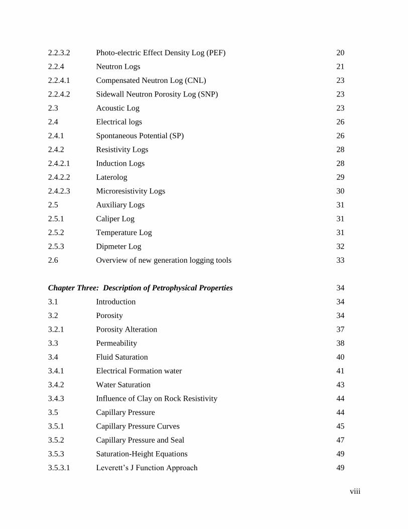
Chapter Three: Description of Petrophysical Properties 34

3.1 Introduction 34

3.2 Porosity 34

3.2.1 Porosity Alteration 37

3.3 Permeability 38

3.4 Fluid Saturation 40

3.4.1 Electrical Formation water 41

3.4.2 Water Saturation 43

3.4.3 Influence of Clay on Rock Resistivity 44

3.5 Capillary Pressure 44

3.5.1 Capillary Pressure Curves 45

3.5.2 Capillary Pressure and Seal 47

3.5.3 Saturation-Height Equations 49

3.5.3.1 Leverett’s J Function Approach 49

ix

3.5.3.2 Johnson Capillary method 50

3.5.3.2 Skelt-Harrison Capillary Pressure and log Based Method 50

SECTION TWO: PETROPHYSICAL EVALUATION

Chapter Four: Wireline Log Editing and Normalization 51

4.1 Introduction 51

4.2 Log data Collection and Creation of Database 53

4.2.1 Wireline logged Intervals for Wells 53

4.3 Log Editing 55

4.3.1 Depth Shifting 55

4.3.2 Borehole environmental correction 56

4.3.3 Mud filtrate Invasion Correction 60

4.3.4 Smoothing, De-Spiking and Noise Removal 62

4.4 Curve Splicing/Merging 63

4.5 Curve Normalization 64

Chapter Five: Core Analysis and Interpretation 68

5.1 Introduction 68

5.2 Conventional Core Analysis 69

5.2.1 Interval Cored 69

5.2.1.1 Well OP1 69

5.2.1.2 Well OP2 71

5.2.1.3 Well OP3 73

5.3 Core-Log Depth Match 75

5.4 Lithofacies Description 76

5.4.1 Well OP1 Lithofacies 78



5.5 Analysis and Interpretation of Results 82

x

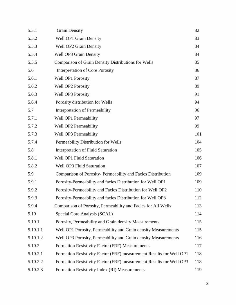
5.5.1 Grain Density 82

5.5.2 Well OP1 Grain Density 83



5.5.5 Comparison of Grain Density Distributions for Wells 85

5.6 Interpretation of Core Porosity 86

5.6.1 Well OP1 Porosity 87



5.6.4 Porosity distribution for Wells 94

5.7 Interpretation of Permeability 96

5.7.1 Well OP1 Permeability 97



5.7.4 Permeability Distribution for Wells 104

5.8 Interpretation of Fluid Saturation 105

5.8.1 Well OP1 Fluid Saturation 106

5.8.2 Well OP3 Fluid Saturation 107

5.9 Comparison of Porosity- Permeability and Facies Distribution 109

5.9.1 Porosity-Permeability and facies Distribution for Well OP1 109

5.9.2 Porosity-Permeability and Facies Distribution for Well OP2 110

5.9.3 Porosity-Permeability and facies Distribution for Well OP3 112

5.9.4 Comparison of Porosity, Permeability and Facies for All Wells 113

5.10 Special Core Analysis (SCAL) 114

5.10.1 Porosity, Permeability and Grain density Measurements 115

5.10.1.1 Well OP1 Porosity, Permeability and Grain density Measurements 115

5.10.1.2 Well OP3 Porosity, Permeability and Grain density Measurements 116

5.10.2 Formation Resistivity Factor (FRF) Measurements 117

5.10.2.1 Formation Resistivity Factor (FRF) measurement Results for Well OP1 118

5.10.2.2 Formation Resistivity Factor (FRF) measurement Results for Well OP3 118

5.10.2.3 Formation Resistivity Index (RI) Measurements 119

xi

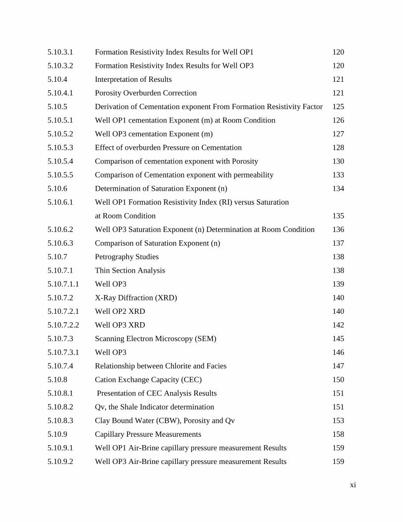
5.10.3.1 Formation Resistivity Index Results for Well OP1 120

5.10.3.2 Formation Resistivity Index Results for Well OP3 120

5.10.4 Interpretation of Results 121

5.10.4.1 Porosity Overburden Correction 121

5.10.5 Derivation of Cementation exponent From Formation Resistivity Factor 125

5.10.5.1 Well OP1 cementation Exponent (m) at Room Condition 126

5.10.5.2 Well OP3 cementation Exponent (m) 127

5.10.5.3 Effect of overburden Pressure on Cementation 128

5.10.5.4 Comparison of cementation exponent with Porosity 130

5.10.5.5 Comparison of Cementation exponent with permeability 133

5.10.6 Determination of Saturation Exponent (n) 134

5.10.6.1 Well OP1 Formation Resistivity Index (RI) versus Saturation

at Room Condition 135

5.10.6.2 Well OP3 Saturation Exponent (n) Determination at Room Condition 136

5.10.6.3 Comparison of Saturation Exponent (n) 137

5.10.7 Petrography Studies 138

5.10.7.1 Thin Section Analysis 138

5.10.7.1.1 Well OP3 139

5.10.7.2 X-Ray Diffraction (XRD) 140

5.10.7.2.1 Well OP2 XRD 140

5.10.7.2.2 Well OP3 XRD 142

5.10.7.3 Scanning Electron Microscopy (SEM) 145

5.10.7.3.1 Well OP3 146

5.10.7.4 Relationship between Chlorite and Facies 147

5.10.8 Cation Exchange Capacity (CEC) 150

5.10.8.1 Presentation of CEC Analysis Results 151

5.10.8.2 Qv, the Shale Indicator determination 151

5.10.8.3 Clay Bound Water (CBW), Porosity and Qv 153

5.10.9 Capillary Pressure Measurements 158

5.10.9.1 Well OP1 Air-Brine capillary pressure measurement Results 159

5.10.9.2 Well OP3 Air-Brine capillary pressure measurement Results 159

xii

5.10.9.3 Well OP2 Mercury-Injection capillary pressure measurement Results 160

5.10.10 Interpretation of Capillary Pressure Results 160

5.10.10.1 Well OP1 Water Saturation determination from Capillary pressure curves 161



5.11 Saturation –Height Determination from Leverett’s J-Function Method 166

Chapter Six: Petrophysical Model of Volume of Shale, Porosity and Water Saturation

from Core and Log

6.1 Introduction 171

6.2 Volume of Shale 171

6.2.1 Gamma-Ray Method 173

6.2.2 Spontaneous Potential (SP) Method 174

6.2.3 Neutron Log Method 174

6.2.4 Resistivity Method 175

6.2.5 Correction of Shale Volume 175

6.2.6 Double Clay Indicators 177

6.2.7 Parameters used for determination of Volume of Clay 178

6.2.8 Calibration of Volume of Clay (Vcl) Models 179

6.2.9 Use of Spectral Gamma-Ray log as an Estimator of Clay type 183

6.3 Porosity Model 186

6.3.1 Porosity Determination from Density Log 186

6.3.2 Porosity from Neutron Log 187

6.3.3 Porosity from Sonic (acoustic) Log (ΦS) 188

6.3.4 Effective Porosity Determination (Φe) 189

6.3.5 Comparison of Log and Core Porosity 190

6.4 Water Saturation Models 195

6.4.1 Parameters 197

6.4.1.1 Formation Temperature Determination 197

6.4.1.2 Determination of formation Water Resistivity (Rw) 199

6.4.1.2.1 SP Method for Formation Resistivity water Estimation 200

xiii

6.4.1.2.2 Pickett Plot method For Formation water Resistivity Estimation 202

6.4.1.3 Cation Exchange Capacity per Pore Volume (QV) and Equivalent

Conductance of Clay Cations (B) 203

6.4.2 Water Saturation (Sw) Models 203

6.4.2.1 Archie’s Model 204

6.4.2.2 The Shaly-Sand Model 205

6.4.2.2.1 The Simandoux Model 205

6.4.2.2.2 Indonesian Model 206

6.4.2.2.3 Waxman-Smits Model 207

6.4.2.2.4 Dual-Water Model 208

6.4.2.2.5 Juhasz Model 211

6.4.3 Comparison of Core and Log Water saturations 211

6.5 Bulk Volume of Water (BVW) 215

Chapter Seven: Permeability, Rock Typing and Flow Units 217


7.2 Permeability 218

7.2.1 Permeability from Core Analysis (Permeability–Porosity Function) 218

7.3 Permeabilities Estimate from Log 223

7.4 Permeability from the Repeat Formation Test (RFT) 229

7.4.1 Relative Permeability 229

7.5 Determination of Rock types (Petrofacies) 233

7.5.1 Well OP1 Petrofacies determination 235



7.6 Comparison of Petrofacies and Lithofacies 240

7.7 K/PHI Relationship 244

7.8 Hydraulic Flow Zone Indicator (FZI) 246

Chapter Eight: Determination of Fluid Contact 258


8.2 Wireline Pressure data analysis and Interpretation 258

xiv

8.2.1 Well OP1 260

8.2.2 Well OP2 261

8.2.3 Well OP3 262

8.2.4 Well OP4 262

8.2.5 Well OP6 263

8.2.6 Well MA1 264

8.2.7 Well MA2 265

8.2.8 Well MA3 266

8.3 Comparison of Log, DST and RFT data fluid contact 269

Chapter Nine: Application of Results, Determination of Cut-Off and Net Pay 278


9.2 Determination of Petrophysical Properties in Non-Cored Wells 279

9.3 Cut-off Determination 287

9.3.1 Porosity Cut-Off Determination 288

9.3.2 Volume of Shale Cut-Off Determination 290

9.3.3 Water Saturation Cut-Off Determination 292

9.4 Determination of Net Pay 293

Chapter Ten: Conclusions and Recommendations 304

References 310

Appendices 324

xv

LIST OF FIGURES

Page No

1.1 Outline of Research 3

1.2 Chronostratigraphic and sequence stratigraphic diagram

of the Orange Basin 6

1.3 Well location map 8

1.4 Section one of the flow chat of research methodology 11

1.5 Section two of Research methodology flow chart 12

2.1 Diagram of GR log 15

2.2 Compton Scattering of Gamma Rays 17

2.3 Density and litho density (photoelectric) logging in relation of

gamma ray energy 18

2.4 Neutron speed versus source (MeV) 22

2.5 The positions of transmitters and Receivers in Sonic tool 24

2.6 Graphics of Self Potential Curve showing Static Self Potential (SSP)

and Shale line 27

2.7 Example of presentation of dip log 32

3.1 Example of pore space and mineral grain space 35

3.2 Example of Effective and total Porosity 36

3.3 Packings of spheres of primary or intergranular porosity 37

3.4 Directions of measurement of permeability 39

3.5 Rock Permeability Ranges 40

3.6 Contact angles for water-wet and oil-wet surfaces 45

3.7 Pressure vs Depth plot 48

4.1 Flow chart of Log editing 52

4.2 Example of gamma-ray log Run at the same depth with other logs 59

4.3 Example of density log affected by borehole 61

4.4 Graphics of uncorrected and environmentally corrected logs 63

4.5 Thin bed Recognition on Resistivity logs 65

4.6 Example of spike and de-spiking of sonic log 66

4.7a Example of Log at different runs (unspliced curves) 67

xvi

4.7b Examples of graphics of spliced curves 68

4.8a GR log values for all Well before Normalization 69

4.8b Possible Reference Wells (OP4 and OP5) used for Normalization 70

4.8c Normalized curves 71

5.1 Example of Log and Core data comparison before depth shifting 79

5.2 Well OP1 showing core facies in track 3 82

5.3 Well OP2 graphics showing Core facies in track 3 83

5.4a Well OP3 core 1 Facies shown in track 3 84

5.4b Well OP3 core 2 Facies shown in track 3 85

5.5 Histogram of Well OP1 Core Grain densities 87

5.6 Grain Density Histogram of Well OP2 88

5.7 Well OP3 core grain density cumulative frequency plot 89

5.8 Grain density histogram plot for all Well 90

5.9a Well OP1 Core Porosity versus depth Plot 92

5.9b Histogram Of porosity distribution of Well OP1 93

5.10a Well OP2 Porosity versus depth plot 94

5.10b Well OP2 core porosity histogram and plot against depth 95

5.11a Well OP3 porosity versus depth plot 96

5.11b Histogram of Well OP3 core porosity distribution 97

5.12a Histogram of Porosity distribution for Wells 98

5.12b Histogram of Core Porosity Shaly/Silt interval for all Well 99

5.12c Histogram of Core Porosity Massive Sands for Wells 100

5.13a Well OP1 Permeability versus depth Plot 102

5.13b Well OP1 Permeability Histogram Plot 103

5.14a Well OP2 Depth versus permeability plot 104

5.14b Well OP2 permeability histogram plot 105

5.15a Well OP3 depth-permeability plot 106

5.15b Well OP3 core1 and 2 Permeability Histogram Plot 107

5.16 Permeability histogram for Wells 108

5.17 Well OP1 Fluid Saturation versus depth plot 110

5.18a Well OP3 core 1 Fluid saturation versus depth plot 111

xvii

5.18b Well OP3 core 2 fluid saturation versus depth plot 112

5.19 Porosity-Permeability and Gamma ray log and Facies Plot for Well OP1 113

5.20 Porosity-Permeability and Facies and GR plot for Well OP2 114

5.21 Porosity-Permeability and Facies GR plot for Well OP3 115

5.22 Porosity-permeability and Facies distribution for Wells 117

5.23a Well OP3 Porosity at Overburden Pressure vs Porosity

at room condition 126

5.23b Formation resistivity factor (FRF) vs Porosity Plot for Well OP1 129

5.24 Plot of Well OP3 FRF Vs Fractional Porosity 131

5.25 Formation Resistivity factor vs Porosity at Overburden pressure 132

5.26 Well OP1 and OP3 cementation versus porosity plot at room conditions 134

5.27 Cementation versus porosity at Overburden condition of Well OP3 135

5.28 Well OP1 and OP3 cementation exponent vs permeability

at room condition 136

5.29 Well OP1 resistivity Index versus water saturation plot 138

5.30 Well OP3 Resistivity Index versus saturation Plot 139

5.31 Resistivity Index versus Saturation plots for Well OP1 and OP3 140

5.32 Well OP3 thin section at depth 3236m and 3283m showing fine grain,

sub angular to angular, and sparely distributed organic matter and

pore filling Chlorite 142

5.33 Whole Rock mineralogy of Well OP2 145

5.34 Whole rock mineralogy of core 1 and 2 of Well OP3 147

5.35 Different ways of Shale distribution in a formation 148

5.36 Example of Well OP3 SEM analysis result 149

5.37 Distribution of chlorite for Well OP2 150

5.38a Well OP3 core 1 Chlorite distribution 151

5.38b Well OP3 core 1 Chlorite distribution 152

5.39 Plot of Qv versus saturation of bound water for all Wells 158

5.40a Plot of Qv versus Total and effective porosities for all Wells 159

5.40b Multi-Well Porosity versus Saturation of bound water plot 160

5.41 Schematic relationship between Capillary pressure curve and

xviii

oil accumulation 164

5.42 Capillary Pressure Curve for Well OP1 165



5.45 Capillary Pressure Curves with Permeability and Porosity 168

5.46 Leverett’s Saturation determination J-Function 171

5.47 J-function curves for Well OP1 and OP3 172

5.48 Saturation-height function for Wells OP1 and OP3 172

6.1a Schematic diagram of variation of sediments with

clay mineral content increasing from left to right 175

6.1b Volume of shale correction chart 179

6.2 Example of Neutron-Density cross plot as clay indicator 180

6.3 Log determined volume of clay overlain with XRD volume of clay

for Well OP2 183

6.4 Log determined volume of clay overlain with XRD volume of clay

for Well OP3 184

6.5 Well OP1Spectral Gamma ray log 187

6.6 Well OP1 potassium/thorium cross plot for identification of clay type 188

6.7 Well OP1 Comparison of log and core porosity 194

6.8 Well OP2 comparison of log and core porosity 195

6.9 Well OP3 comparison of log and core porosity 196

6.10 Multi-Well overburden porosity versus log porosity 197

6.11 Example of Resistivity of water from SP method 204

6.12 Pickett Plot for determination of resistivity of water (Rw) for

Well OP1, OP2, and OP3 respectively 205

6.13a Estimate of Resistivity of shale (Rsh) from Wells 209

6.14 Comparison of core and log determined bound water saturation

for Well OP1 212

6.15 Comparison of core and log estimated bound water saturation and

XRD mineralogy data for Well OP2 213

6.16 Comparison of Core and log water saturation models for Well OP1 215

xix

6.17 Comparison of Core and log water saturation models for Well OP3 217

6.18 Bulk Volume of water and Effective Porosity Plot for Well OP3 219

7.1 Porosity –Permeability Cross Plots for determination of function 222

7.2 Well OP1 Plot of Predicted Permeability Overlaying original core

permeability in track 4 223





7.5 Example of irreducible water saturation estimate point from

capillary pressure measurement 227

7.6 Log estimated permeability and overlaid core permeability for Well OP1 229



7.9 Relative Permeability curves for Well OP2 and OP3 within the reservoir

intervals 233

7.10 Comparison of permeabilities derived from log, RFT and Krh equations

for Well OP2 234

7.11 Comparison of Permeabilities derived from core, log and cross plot 235

7.12 Correlation of Winland and Pittman’s plots for Well OP1 239



7.15a Comparison of lithofacies and Petrofacies for Well OP1 244

7.15b Comparison of Lithofacies and Petrofacies for Well OP2 245

7.15c Comparison of lithofacies and Petrofacies for Well OP3 246

7.15d Comparison of lithofacies and Petrofacies for entire Well 247

7.15e Permeability/Porosity Ratio (K/PHI) for Wells 248

7.16a Well OP1 Flow Zone Indicator, Rock Types and Facies plot 253

7.16b Well OP1 NPI Vs RQI Plot 254


7.17b Plot of NPI Versus RQI for Well OP2 256

xx


7.18b Plot of NPI Versus RQI for Well OP3 259

7.18c Plot of NPI Versus RQI for all Wells 260

8.1 Well OP1 Pressure versus depth Plot for identification of

Gas/Water Contact (GWC) and Fluid densities 263

8.2 Well OP2 Pressure versus Depth Plot 264

8.3 Well OP3 Pressure Versus Depth Plot showing possible GWC

at measured depth 3361.3m 265



8.6 Well MA1 Pressure versus Depth Plot 268



8.9 Overlaid gas and water gradients in the field 271

8.10 Well OP1 comparison of log and Pressure data Gas Water Contact 273

8.11 Well OP3 Comparison of Log and Pressure data Gas water Contact 274

8.12 Well OP4 Comparison of Log and Pressure data Gas Water Contact 276

8.13 Well OP6 Comparison of Log and Pressure data Gas Water Contact 277

8.14 Well MA 2 Comparison of Log and Pressure data Gas Water Contact 278

8.15 Well MA3 Comparison of Log and Pressure data Gas water contact 279

9.1 Well MA1 results estimated petrophysical properties 283

9.2 Well MA2 results of estimated of Petrophysical Properties 284

9.3 Well MA3 Results of Estimated Petrophysical Properties 285

9.4 Well MA4 Results of Estimated Petrophysical Properties 286

9.5 Well OP4 Results of Estimated Petrophysical Properties 287



9.8a Multi-Well Porosity-Permeability Plot for Cut-Off determination 291

9.8b Multi-Well Permeability and Porosity Histogram distributions 292

9.8c Application of Permeability and Porosity Cut-Off to Petrofacies 293

9.9a Volume of shale versus porosity and gamma-ray log plot 294

xxi

9.9b Multi-Well Vclay frequency distribution and cut-off point 295

9.10 Multi-Well Porosity vs Water Saturation and Frequency Distribution 296

9.11 Well OP1 showing Calculated Reservoir Parameters and Pay Flags 298

9.12 Well OP2 showing Calculated Reservoir Parameters and Pay Flag 299

9.13 Well OP3 graphics of Calculated Reservoir Parameters and Flags 300

9.14 Well OP4 showing calculated reservoir parameters and Flags 301

9.15 Well OP5 showing Calculated Reservoir Parameters and Flags 302

9.16 Well OP6 showing calculated Reservoir Parameters and Flags 303

9.17 Well MA2 Showing Calculated Reservoir Parameters and Flags 304

9.18 Well MA3 Showing Calculated Reservoir Parameters and Flags 305

9.19 Well MA4 Graphics of Calculated Reservoir Parameters and Flags 306

xxii

LIST OF TABLES

Page No

1.1 Summary of data used for study 10

2.1 Depth of investigation of density tool and typical readings 19

2.2 Photo-electric absorption factor for common minerals 21

2.3 Typical Sonic matrix travel times of some rocks 26

2.4 Curve names and mnemonics of laterolog 29

2.5 Common curve names of microresitivity logs 30

3.1 Cementation of various rock types 42

3.2 Interfacial Tension and Contact Angle Values 47

4.1 Suite of Logs Run in wells at various Intervals 54

4.2 Summary of environmental corrections applied to logs 57

4.3 Guide for borehole condition 58

5.1 Well OP1 Routine Core Analysis 70

5.2 Well OP2 Routine core analysis results 72

5.3 Well OP3 core1 analysis results and lithology description 73

5.4 Well OP3 core 2 Routine core analysis results and lithology description 74

5.5 Cored Intervals and Core-log Shift Summary for Wells 76

5.6 Lithofacies descriptions and classification of Reservoir Facies 78

5.7 Matrix density of common lithology 82

5.8 Permeability classification scale 98

5.9 Porosity, Permeability and Grain Density test results of

Well OP1 at room condition 115

5.10 Porosity, Permeability and Grain Density test results of

Well OP3 at room condition 106

5.11 Result of Well OP1 FRF measurement at room condition 118

5.12 Result of Well OP3 FRF measurement at room and overburden conditions 118

5.13 Resistivity Index results for Well OP1 119

5.14 Resistivity Index results for Well OP3 120

5.15 Well OP3 core 2 data used for porosity overburden correction 121

xxiii

5.16 Wells OP1, OP2 and OP3 calculated Overburden Corrected Porosities 123

5.17a Classification of Cementation exponent 124

5.17b Cementation exponent (m) from Formation resistivity factor measurement 125

5.18 Cementation exponent for Well at Room Condition 126

5.19 Well OP3 cementation exponent at overburden pressure (4,830 psi) 128

5.20 Well OP3 comparison of cementation exponents 129

5.21 Well OP1 result of resistivity index measurements and n values 134

5.22 Well OP3 Result of Saturation exponent (n) derived from RI vs Saturation 136

5.23 Whole rock Mineralogy of Well OP2 140

5.24 Whole Rock Mineralogy of Well OP3 142

5.25 Result of Cation Exchange Capacity (CEC) for Wells 150

5.26 Calculated values of cation exchange capacity per pore volume for Wells 151

5.27 Calculated effective porosity and clay bound water for Wells 153

5.28 Well OP1 Capillary Pressure test data 158

5.29 Well OP3 Capillary Pressure test data 159

6.1 Summary of Parameters used for Volume of Clay calculations 181

6.2 Summary of Parameters used for log Effective porosity calculation 192

6.3 Calculated Formation temperature (T2) and Resistivity of mud filtrate 201

7.1 Established Porosity-Permeability Functions for Wells 222

7.2 Classification of Rock Types 7.3 237

7.3 Rock types classification based on winland and Pittman calculations 238

7.4 Rock types classification based on winland and Pittman calculations

for Well OP2 240

7.5 Reservoir rock classifications of Well OP3 242

7.6 Well OP1 Calculated values for RQI, NPI and FZI 251



8.1 Ranges of density and pressure gradients for hydrocarbon 262

8.2 Summary of pressure gradients and densities for Wells 270

8.3 Summary of Gas Water Contact 280

9.1 Well OP1 Summary of calculated Reservoir Pay Parameters 297

xxiv

9.2 Well OP2 Summary of Calculated Reservoir Pay Parameters 299





9.7 Well MA2 Summary of calculated Reservoir Pay Parameters 304



xxv

LIST OF APPENDICES

Page No

Appendix A Logging tool code and tool description 327

Appendix B Core photos 328

Appendix C Well resistivity index vs saturation plot 330

Appendix D Well OP2 capillary pressure data 337

Appendix E Well J-Function and height parameters 338

Appendix F Neutron versus Density and GR log plots 340

Appendix G Log versus Core overburden Porosity for Wells 341

Appendix H Pickett plot for Wells 342

Appendix I Results of RFT measurements for Wells 343

1

CHAPTER ONE

INTRODUCTION

1.1 BACKGROUND INFORMATION

Petrophysics is regarded as the process of characterising the physical and chemical

properties of the rock-pore-fluid system through the integration of the geological

environment, well logs, rock and fluid sample analyses and their production histories.

A reservoir is a subsurface layer or a sequence of layers of porous rock that contain

hydrocarbon. Depending on their geological origin, these layers are usually sandstone

rock or carbonate rock. The hydrocarbon resides in the open spaces in the rock matrix

called pores. The parameters that determine the behaviour of pore system are known

as the petrophysical properties.

In reservoir evaluation and development, the assessment of petrophysical properties

such as porosity, permeability, and water saturation, percentage of shale volume,

mineralogy, and type of pore fluid are deduced from well logs, core analysis, and well

tests. The successful evaluations of these properties are necessary for determining the

hydrocarbon potential of a reservoir system performance and also help us predict the

behaviour of complex reservoir situations. The integration of comprehensive

mineralogical studies with the evaluation of petrophysical properties provides a

valuable basis for reservoir systems studies. Thus, it aids in understanding the

influence of minerals in rock properties when correlated with wire line geophysical

logs. The operators in the Petroleum Industry need quick and reliable methods by

which the fundamental properties of the rocks and the fluid contents can be

determined in the subsurface. This is easily achieved by the use of wire line

geophysical logs.

Geophysical logs are not direct measures of the petrophysical properties of the

formation. The logs measure different formation parameters that are then translated to

properties of geological significance during log interpretations. The parameters

measured by the logs may be inherent to the formation itself such as the formation

resistance to an electric current. Logs also measure mechanical parameters in the

2

borehole such as the hole diameter and the down hole temperature. The petrophysical

properties determined from cores and logs are not always comparable, hence

considerable care must be observed when comparing data from core and log analysis.

Core analysis is one of the reservoir assessment tools that directly measure many

important formation properties. The analysis determines porosity, permeability, grain-

size distribution, grain density, mineral composition, sensitivity of fluids, and effect of

overburden stress (Bateman, 1985).

The Albian reservoir intervals in the Orange Basin consists of an overall association

of coursing-upward, laminated and bioturbated mudstone to massive and planar cross-

bedded sandstones with evidence of reducing conditions. The reservoirs are

heterogeneous consisting of massive sands and are encountered at depths below

2700m with varying thicknesses.

The Albian age gas bearing reservoir sandstones evaluated in this study range

between 2800m to 3500m depending on the position of the well. The study area is

zoned into two. The MA wells in the Northern part of the field and the OP wells in the

central and southern part of the study area. Ten wells are the focus of the study, of

which three (OP1, OP2 and OP3) were regarded as the key wells because core

analysis was performed in some of the reservoir sections of these wells.

1.2 APPROACH AND OUTLINE OF THE THESIS

This thesis started with the review of previous studies and literature search in

comparable oil and gas fields. This is to get familiarize with the basin architecture,

tectonic and structural features, sediment source and transport history, flow units and

inter play of accumulation. Emphasis has been placed on classic reservoirs because

the techniques that were developed in this study focus on sandstone and shale

lithology.

The petrophysical evaluation approach adopted in this study is a probabilistic log

analysis technique which takes all continuous log data and uses the response to create

an answer. The answer which yields the least difference between the raw and re-

computed logs from that answer is chosen. Core and production data are used to

calibrate the answer derived from the log by adjusting in order to obtain better

performance.

The thesis is grouped into two sections which are depicted in Figure 1.1 below.

3

THESIS STRUCTURE

Section one (Basic concepts)

• Chapter one (Introduction)

• Chapter two (Wireline logs)

• Chapter three (Petrophysical properties)

Section two (Petrophysical evaluation)

• Chapter four (Log editing and normalization)

• Chapter five (Core analysis and interpretation)

• Chapter six (Calibration of volume of shale, porosity and water saturation)

• Chapter seven (Permeability, petrofaciesand flow zone indicators)

• Chapter eight ( Fluid contact determination)

• Chapter nine ( Application of results, cut-off and net pay determination )

• Chapter ten (conclusions and recommendations).

Figure 1.1: Outline of Research.

In petroleum evaluation, the importance of mineralogical studies has been

demonstrated in the northern North Sea where porosity evaluation from logs was

complicated by radioactive and heavy minerals and the evaluation had to resort to an

integrated approach with core and log analysis (Nyberg et al, 1978). The integrated

analysis and interpretation of core and log information together with fluid and

pressure analysis, by geologists, petrophysicists and reservoir engineers has resulted

in a valuable base for field development studies, particularly in circumstances where

major investment decisions are taken with the benefit of few appraisal wells (Hurst &

Archer, 1986).

Petrophysical properties are derived from individual characteristics of the mineral

constituents forming the rock (Serra, 1986), but the mineral themselves are seldom

considered in the evaluation of rock properties. Laboratory studies of sandstones

showed the various petrophysical properties, such as density, radioactivity, resistivity,

porosity, magnetic susceptibility, might vary considerable depending on clay and

heavy minerals, carbonaceous matter and on rock fabrics (Emerson, 2000).

4

The geochemistry of sandstone digenesis is routinely applied to problems of reservoir

simulation and enhances recovery (Hearn et al., 1984). Clay minerals affect all log

measurements and logs have potential for determining clay mineralogy. However, the

sensitivity of logs to mineralogy requires that log responses be calibrated for

mineralogy effects (Patchett & Coalson, 1982; Suau & Spurlin, 1982).

Mineralogy input into geophysical analysis has also provided porosity evaluation

results that are more comparable with direct measurements carried out on core

samples (Guest, 1990).

Saturation profiles can also be used to understand the distribution of water saturation

within a field or prospect Hartmann & Coalson (1990) showed how cores and logs

from four field wells of the Sorrento field, southeast Colorado was determined

through saturation profiles. Bastia (2004) in his study of the depositional model and

reservoir architecture of tertiary deep water sedimentation, Krishna Godavari offshore

Basin, India, reveal that the reservoir of the gas field tertiary sands originally

deposited in the deep water channel-levee system with relatively clean channel and

laminated levee facies as shown in his study.

Core analysis has evolved from qualitative geology descriptions to the use of

sophisticated analysis tool, such as the scanning electron microscopy (SEM), energy

dispersive x-ray spectrometry, x-ray diffraction, infrared spectroscopy, and imaging

analysis techniques Juhasz (1990)

Mineralogical techniques have shown that small variations in the clay mineral content

and rock texture can have an influence on the permeability and on different

geophysical log responses Hurst & Archer (1986). It has thus been suggested that log

derived mineralogical evaluation might be used in conjunction with mineralogical

analysis of core samples in order to validate the quantification from logs, and provide

additional information on mineral texture and distributions.

5

1.3 GEOLOGICAL OVERVIEW

The Orange Basin extends along the coast of Western Africa for 1500 km from the

Aguilhas Arch in the south to the Walvis Ridge in the north. The Basin is one of the

most lightly explored passive margin systems in the world with the South African

portion of the basin encompasses 130,000 km² with water depths ranging to greater

than 3000m. More than 75% of the prospective area is in water depths shallower than

500m and half of the prospective region lies in water depths shallower than 250m. To

date only 47 wells have been drilled in the basin. This exploration effort has lead to

the discovery of one gas field in Namibian waters (Kudu) and one gas field in South

African waters.

Deposition in the area took place in an overall shallow marine shelf-type environment.

Sand deposition mostly resulted from wave reworked dominated delta front and shelf

marine and storm bars. The sandstones are appears greenish which is indicative of the

presence of glauconite marine conditions. The greenish sandstones are massive and

exhibit a wave influenced type of lamination. The sandstones are generally well sorted

ranging in grain size from very fine to medium. The lower and upper contacts of the

sandstones are characterized by an abrupt lower contact, gradual, bioturbated upper

contact Petroleum Agency Brochure (2000).

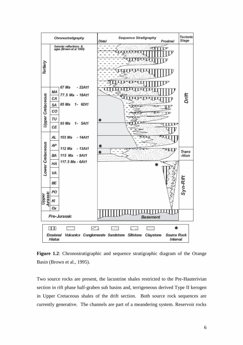
Earliest sedimentation is dated as pre-Hauterivian and likely began in the

Kimmeridgian or Tithonian (~152-154 Ma), although fossil control in the older rocks

is absent due to the lack of marine facies in Wells drilled to date (Figure 1.2).

6

Figure 1.2: Chronostratigraphic and sequence stratigraphic diagram of the Orange

Basin (Brown et al., 1995).

Two source rocks are present, the lacustrine shales restricted to the Pre-Hauterivian

section in rift phase half-graben sub basins and, terrigeneous derived Type II kerogen

in Upper Cretaceous shales of the drift section. Both source rock sequences are

currently generative. The channels are part of a meandering system. Reservoir rocks

7

in the rift section are fluvial and deltaic sandstones and conglomerates derived from

the Palaeozoic Karoo section and underlying basement. Drift sequence reservoir

facies on most of the broad shelf are primarily fluvial sandstones and floodplain

deposits (Jungslager, 1999).

Numerous play types are present in the area. The rift plays are presented by possible

lacustrine sandstones trapping oil from organic rich claystones .The other major play

is represented by synrift sediments and drift plays which include the early cretaceous

Aeolian sandstone play, the Albian incised valley play, structural plays in younger

shelf sediments and deeper water plays comprising roll-over anticlines in growth fault

zones (Vander Spuy, 2002).

Detailed mapping of the numerous reservoir channels at Ibhubesi field, Orange Basin

South Africa necessitated the building of a stratigraphic framework within the Albian

section. This framework was derived from a sequence stratigraphic study of the

Orange Basin by Brown et al which the area was referred as series of incised valley

fill sequences (Brown et al., 1995).

1.4 LOCATION OF STUDY/ WELL LOCATIONS

The study area is located within Orange Basin, Offshore South Africa (Figure 1.3)

below. Ten (10) exploration wells located within the O-M field is the focus of the

work. The field (O-M) and well names used in this study are imaginary names of gas

field and wells located in the Orange Basin South Africa. The wells are as follows:

OP1

OP2

OP3

OP4

OP5

OP6

MA1

MA2

MA3

MA4

8

Figure 1.3: Well Location map

9

1.5 AIMS AND OBJECTIVES

The research is aimed at evaluating the reservoir potentials of O-M field, Offshore

South Africa with limitation to the available data. This could be achieved through the

integration and critically comparing results from core analysis, petrography studies for

evaluating and correcting key petrophysical parameters obtained from wireline logs

and generates an effective static reservoir model.

The specific objectives include the following:

Editing and normalization of raw wireline log data.

Classification of lithofacies, petrofacies and flow zone indicators

Calibration of logs/ core data to obtain parameters for petrophysical log

interpretations.

Integrated studies of Sedimentology and petrophysics to determine the

percentages of clay, type and distributions within the reservoir sections and its

effect on water saturation.

Determination of Porosities from logs

Determination of true formation resistivity water and accurate estimate of

bound and free water saturations.

Determination of water/oil/gas contacts from water saturation calculations and

Repeat Formation Tests (RFT)

1.6 RESEARCH METHODOLOGY

This process started with review of previous studies and utilizes the probabilistic

Petrophysics log analysis approach for multi-mineral evaluation for a static reservoir

model. This method takes all continuous log data and response equations to the

proposed formation components and computes an answer. Core and production data

are used to adjust this answer to produce a conceptual static petrophysical model.

Demonstrations will be carried out on integration of different subsurface data at

relevant and appropriate scales in order to construct reliable static reservoir models.

The Table below present summary of data used for this study:

10

Table 1.1: Summary of data used for study

Well

Name

Conventional

Logs

Conventional

Core

Special

Core

Analysis

Petrography

RFT DST Completion

Report

MA1 X X X

MA2 X X X

MA3 X X X

MA4 X X

OP1 X X X X X

OP2 X X X X X

OP3 X X X X X X X

OP4 X X

OP5 X

OP6 X X

A conventional suite of open-hole wireline logs were run by Schlumberger in all the

wells. The main measurements acquired in all the wells at different Runs include:

Gamma-Ray, Caliper, Spontaneous Potential

Porosity Logs – Density, Neutron and sonic

Resistivity Logs- Deep Induction, Spherically focused Laterolog, Micro-

Spherically focused logs.

The collected data was first edited /reviewed and then loaded into the database for

petrophysical modeling at different stages.

The flow charts (Figures 1.4, 1.5) below represent summary of workflow which starts

from data collection and terminates at submission of report.

11

Figure 1.4: Section one of the flow chat of research methodology.

Data

collection

Wireline

Logs Core data Geological

Setting

Well test

reports

Load to

workstation Thin section Petrography.

XRD,SEM

Top of the Zones/Facies

DST and

RFT

Depth

Control

Editing and

Normalization

De-Spiking

Splicing/Generating

Final LAS files

Routine Analysis

and SCAL

Core Petrophysical

Model

12

Figure 1.5: Section two of Research methodology flow chart.

PETROPHYSICAL

MODELING

Lithology

Determination

Porosity

Model

Water

Saturation

Permeability

Core Logs

Conventional/

SCAL

GR, RHOB, PEF,

NPHI, SP, ILD,

Petrography vclay/log vclay

Calibration

Core Log

Overburden

Correction

RHOB

NPHI

DT

Core/log porosity

Effective porosity

Capillary

Pressure

Log

Rw

Sw

Swirr

Core Log

Calibration/ Overburden

Calibration

Fluid Contacts, Cut-Off and Net Pay

13

CHAPTER TWO

WIRELINE LOGGING

2.1 INTRODUCTION

Wireline logging is a process that depends on lowering the logging cable into a drill

well by loggers for the measurements of physical, chemical, electrical, or other

properties of rock/fluid mixtures penetrated by drilling a well into the Earth‟s mantle.

Well logging is usually carried out with instruments that are either suspended from a

steel cable (wireline) or embedded in the drill string (logging while drilling, LWD).

The wireline log is a graph and the data are continuous measurements of a log

parameter against depth. When a log is made, it is said to be RUN. A log run is made

at the end of a drilling phase and before casing is put in the hole and each of the run is

numbered being counted from the first time that the particular log is recorded.

When logs are used for purposes other than evaluation of oil and gas, they are often

called geophysical logs instead of well logs. The science is called borehole geophysics

instead of petrophysics. The theory of well logging remains the same just the

nomenclature and sometimes the emphasis (Rider, 1996).

The geophysical well logging was first developed for the petroleum Industry by

Marcel and Conrad Schlumberger in 1927. The Schlumberger brothers developed a

resistivity tool to detect differences in the porosity of the sandstones of the oilfield at

Merkwiller- Pechelbronn in eastern France (Schlumberger, 1989).

The wireline logging can be grouped into two. They are the open-hole and cased- hole

logging. The open-hole logging is based on measurements of the formations electrical,

acoustic, and nuclear properties. Cased-hole logging includes measurements of

nuclear, acoustic and magnetic properties. The open-hole logging will be the focus of

this research. Some well logs are made of data collected at the surface; examples are

the core log, mud sample logs, drilling time logs, etc.

Wireline logging is the established way of gathering about hydrocarbon bearing

reservoirs over the length of the well and the objective is to obtain information on

hydrocarbon. Physical properties such as resistivity, density, natural gamma radiation,

and magnetic resonance are recorded as a function of depth. These physical properties

are converted into petrophysical properties of the rock.

14

The wireline logging tools can be grouped into active and passive tools. The active

tools measure the response of formation to some form of excitations. Examples

include density, neutron, resistivity, and the nuclear magnetic resonance (NMR) tools.

The passive tools measure natural occurring phenomenon such as the gamma

radiation that is emitted by elements in the rock or electric potential caused by

difference in salinity of the mud in the well and the formation water. Examples

include gamma ray (GR) and Spontaneous Potential (SP) logs.

2.2 THE NUCLEAR LOGS

The Nuclear logs record radioactivity that may be either naturally emitted or induced

by particle bombardment. Radioactive materials emit alpha, beta and gamma

radiation. Only the gamma radiation has sufficient penetrating power to be used in

well logging. Neutrons are used to excite atoms by bombardment in the well logging.

They have high penetrating power and are only significantly absorbed by hydrogen

atoms. The hydrogen atoms in the formation fluids are very effective in slowing

neutrons and thus tend to be an important property in well logging.

The basic nuclear logs that will be discussed briefly are the following:

Conventional Natural Gamma-Ray (GR)

Spectral Gamma-Ray (SGR)

Formation Density (RHOB)

Photoelectric Effect (PEF)

Compensated Neutron (CNL)

Sidewall Neutron Porosity (SNP)

2.2.1 Conventional Natural Gamma-Ray Log (GR)

The natural radiation is due to the disintegration of nuclei in the subsurface.

Potassium, Thorium and Uranium are the major decay series that contribute to natural

radiation. These elements Potassium, Thorium and Uranium tend to be concentrated

in shales, and are present in feldspars and micas that occur in many sandstone

reservoirs.

The gamma-ray log is a log of this naturally occurring radiation. The units are

American Petroleum Institute (API).Clean sands has fairly low levels of <45 API and

shales has high gamma reading > 75 API. The measurements are used to calculate the

15

amount of shale as a function of depth and the vertical resolution of the tool is

approximately 0.6m with a depth of investigation of 0.15 – 0.3m depending on the

density of the rock. The gamma ray log is used for basic lithology analysis,

quantitative estimation of clay content, correlation of formations, and the depth

matching of multiple tool runs.

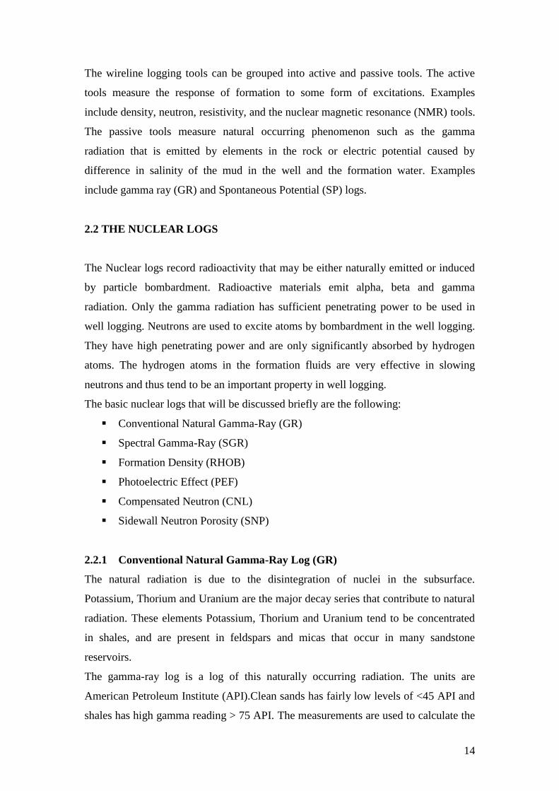
The simple gamma ray log is usually recorded in track one and scales chosen locally,

but 0 – 100 and 0 – 150 API are common. A deflection of GR log to the right

indicates shales, where the maximum and constant recorded radioactivity to the right

shows shale line. A deflection to the left indicates sandstone, where the maximum and

constant recorded radioactivity to the left shows sandstone line as indicated in Figure

2.1 below.

Figure 2.1: Diagram of GR log (Modified after Russel, 1944).

0 150 API

16

In the conventional gamma sonde, a scintillation counter detects total disintegration

from sources in the radial region close to the hole. The scintillation detector uses a

sodium iodide crystal coupled to a photomultiplier tube to detect tiny flashes of light

associated with penetrations of the crystal by gamma rays.

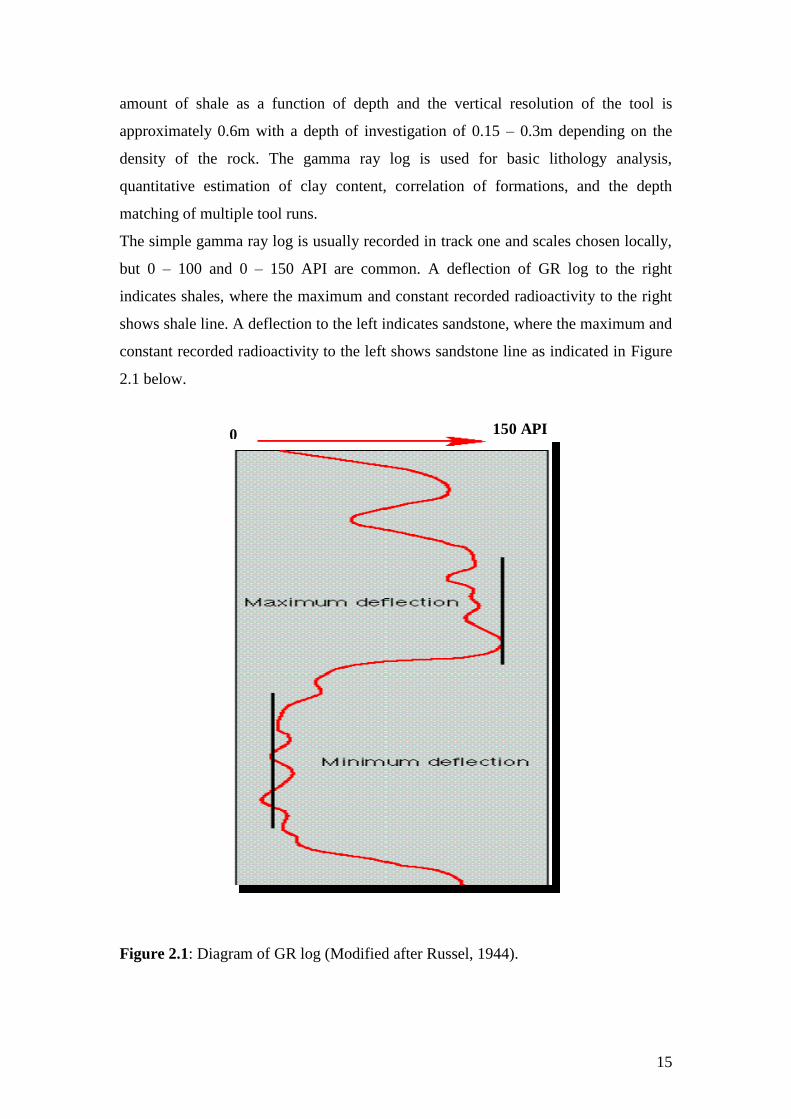
2.2.2 Spectral Gamma Ray (SGR)

The spectral gamma ray log record individual responses for potassium, thorium and

Uranium bearing minerals. The detectors record radiation in several energy windows

as Gamma-Ray – Potassium, Gamma-Ray- Thorium, and Gamma-Ray-Uranium. In

the three window tool, estimates of the concentrations of the three radioactive

elements can be made as follows:

Potassium: Gamma Ray Energy 1.46Mev (K40)

Thorium Series: Gamma Ray Energy 2.62 MeV (T1205)

Uranium-Radium Series: Gamma Ray Energy 1.76 MeV (Bi214)

Spectral gamma sondes also provide a total GR counts from a fourth window that is

equivalent to a conventional gamma log. The main applications of spectral gamma

logs are:

Clay Content Evaluation – Spectral logs will distinguish between clays and

other radioactive minerals such as phosphate.

Clay type identification – Ratios such as Th: K are used to distinguish

particular clay minerals.

Source Rock Potential – There is an empirical relationship between U: K

ratios and organic carbon in shales.

2.2.3 Density Logs

Density logging employs incident gamma radiation which results in two important

interactions with the electron cloud and its parent atoms which are the Compton

scattering and photo-electric absorption. The density logging techniques are the Bulk

electron density and the photo-electric density.

Compton scattering allows the measurement of bulk density based on electron

concentration moderating the gamma flux. The Photo-electric response occurs at

17

lower energies where gamma rays are absorbed by atoms which then eject secondary

gamma rays. The low energy portion of the spectrum is dominated by the PE effect.

The source emits high energy gamma rays that pass through the formation until they

are scattered (Compton scattering) and then eventually captured (Absorbed) having

lost most of their energy. Two sodium iodide detectors are placed within the cloud

capturing a portion of the scattered rays and counting them (Figure 2.2).

Figure 2.2: Compton scattering of gamma rays.

The count rate at each detector is proportional to the electron density of the rock and

is proportional to the bulk density. The radioactive source most often used in density

logging is the isotope Cs137. This is because it has energy of 662 KeV in the centre of

the range of energies where the probability of Compton scattering is highest (Figure

2.3 below).

A density log is a measure of the number of low energy gamma rays surrounding the

sonde which is due to elastic scattering and is proportional to the electron density of

the rock. We actually measure electron density but what is needed is the bulk density

of the rock, therefore the ratio of atomic number and weight are important.

The density tools use a gamma ray source and three gamma ray detectors. The number

of gamma rays returning to the detector depends on the number of electrons present

18

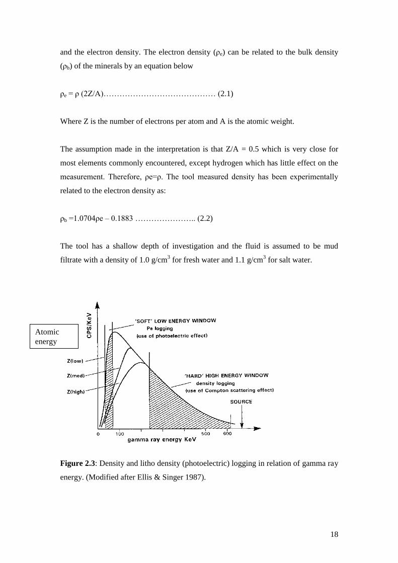
and the electron density. The electron density (ρe) can be related to the bulk density

(ρb) of the minerals by an equation below

ρe = ρ (2Z/A)…………………………………… (2.1)

Where Z is the number of electrons per atom and A is the atomic weight.

The assumption made in the interpretation is that Z/A = 0.5 which is very close for

most elements commonly encountered, except hydrogen which has little effect on the

measurement. Therefore, ρe=ρ. The tool measured density has been experimentally

related to the electron density as:

ρb =1.0704ρe – 0.1883 ………………….. (2.2)

The tool has a shallow depth of investigation and the fluid is assumed to be mud

filtrate with a density of 1.0 g/cm3 for fresh water and 1.1 g/cm

3 for salt water.

Figure 2.3: Density and litho density (photoelectric) logging in relation of gamma ray

energy. (Modified after Ellis & Singer 1987).

Atomic

energy

19

2.2.3.1 Formation Bulk Density Log (RHOB)

The density log is a continuous record of formation bulk density. This is the over all

density of a rock including solid matrix and the fluid enclosed in the pores. The unit

of bulk density measurement is gram per centimetre cubed (g/cm3).

The density log is normally plotted on a linear scale of bulk density and run in tracks

two and three most often with a scale between 2.0 and 3.0 g/cm3 (Rider, 1996). Table

2.1 present density parameters.

Table 2.1: Depth of investigation of density tool and typical readings

Density Parameters

Standard

Depth of investigation

18 inches

6 inches Vertical resolution

6‟ to 9 inches

Limestone (0%)

Sandstone (0%)

Dolomite (0%)

Anhydrite

Salt

2.71

2.65

2.87 Reading in Zéro porosity

2.98

2.03

Shale

Coal

2.2-2.7

1.5+ Typical Readings

The density tool is extremely useful as it has high accuracy and exhibits small

borehole effects. The major uses are in the determination of porosity as given below :

Determination of porosity-

)3.2.........(fma

bma

20

Where:

Φ = Porosity

ρ ma =matrix density

ρ b =density from log

ρ f =Fluid density of the mud filtrate

The other uses of the density log are:

Lithology identification in combination with Neutron tool

Gas indication in combination with Neutron tool

Formation acoustic impedance in combination with Sonic tool

Shaliness of formation in combination with Neutron log

2.2.3.2 Photo-electric Effect density Log (PEF)

The photo-electric effect log is influenced more by atomic number than by electron

density. The photo-electric effect only occurs at low energy; generally below 100KeV

(Figure 2.3).It measures the absorption of low energy gamma rays by the formation

and is calibrated into units of barns per electron.

The logged value is a function of the aggregate atomic number of all the elements in

the formation and so is a sensitive indicator of mineralogy. The log is less sensitive to

porosity and caving effects since hydrogen has a very low atomic number. The Pho-

electric response depends on the atomic number of the elements in the formation and

varies according to the chemical composition. The photoelectric effect log provides a

direct indication of lithology. The Table below present the photoelectric absorption

factors (Pe) for common sedimentary minerals.

21

Table 2.2: Photo-electric absorption factor for common minerals

2.2.4 Neutron Logs

The Neutron log was introduced commercially by Well Surveys Incorporated two

years after the gamma ray log. Gus Archie working for Shell used the neutron

porosity log in his equation of 1942.

In Neutron logging, fast neutrons are emitted by a chemical source (Americium-

Beryllium) in the sonde and travel through the formation where they are slowed

mainly by collision with hydrogen atom. Slow neutrons are captured by the atoms

with the emission of a gamma ray at various energies and velocities as indicated in

Figure 2.4 below:

22

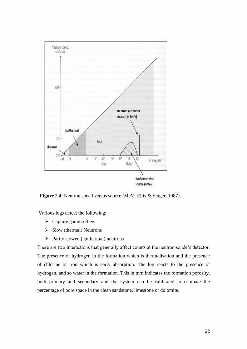
Figure 2.4: Neutron speed versus source (MeV; Ellis & Singer, 1987).

Various logs detect the following:

Capture gamma Rays

Slow (thermal) Neutrons

Partly slowed (epithermal) neutrons

There are two interactions that generally affect counts at the neutron sonde‟s detector.

The presence of hydrogen in the formation which is thermalisation and the presence

of chlorine or iron which is early absorption. The log reacts to the presence of

hydrogen, and so water in the formation. This in turn indicates the formation porosity,

both primary and secondary and the system can be calibrated to estimate the

percentage of pore space in the clean sandstone, limestone or dolomite.

23

2.2.4.1 Compensated Neutron Log (CNL)

The compensated Neutron log (CNL) tool has two detector spacings and is sensitive

to slow neutrons. The tool detects thermal neutrons. The logs can be run in open and

cased holes.

2.2.4.2 Sidewall Neutron Porosity Log (SNP)

The sidewall neutron porosity tools is a single detector pad tool that detect partly

slowed epithermal neutrons. All neutron tools can be run in cased holes to determine

formation porosity. Corrections must be made for the presence of casing and cement

(Krygowski, 2003).

Principal uses of the Neutron logs are listed below:

Porosity display directly on the log

Lithology determination in combination with Density and Sonic logs

Gas indication in combination with Density log

Clay content estimation with gamma Ray log

Correlation in open or cased holes

2.3 ACOUSTIC (SONIC) LOG

The traditional sonic logging involves just the compressional wave measurement done

in the sonde in real time and converted to velocity for lithology, seismic and

geotechnical applications. The sonic log provides a formation‟s acoustic interval

travel time, designated Δt. The travel time or slowness of a sonic primary (P) or

compressional wave through rocks varies due to rock type, compaction. The P-wave

is a refracted wave that passes through the rock mass. It is a fast wave and the first

arrival at our receivers so it is easy to discriminate.

The sonic tools create an acoustic signal and measure how long it takes to pass

through a rock by simply measuring this time we can get an indication of the

formation properties. The amplitude of the signal will also give information about the

formation. The tool uses a pair of transmitters and four receivers to compensate for

24

caves and sonde tilt. The normal spacing between the transmitters and receivers is

about 3 to 5 inches. The diagram (Figure 2.5) below presents the configuration.

.

Figure 2.5: The positions of transmitters and receivers in sonic tool.

The figure above presents a simple tool that uses a pair of transmitters and four

receivers to compensate for caves and sonde tilt. The normal spacing is between 3 to 5

inches. The configuration produces a compressional slowness by measuring the first

arrival transit times.The sonde is centralised and run at about 6 metres per minutes in

water while transmitting at 10 times per seconds at 20 kHz. Each arrival at a receiver

generates a voltage whose first arrival within a prescribed time gate is discriminated.

Noise and cycle skips result in spikes on the log but a de-spiker in the sonde removes

most of these spikes.

The sonic log in sedimentary rocks is considered a porosity log and can generate a

sonic based sandstone or limestone porosity log to compare with those created from

neutron and density logs. No calibration is necessary because it relies on a fixed,

perfectly spaced geometry. The sonic log will display raw transmit times in micro-

25

seconds per foot. The most common interval transit times fall between 40 and 140 ms.

The sonic log is presented in tracks 2 and 3. The major uses are listed below:

Correlation.

Porosity.

Lithology.

Seismic tie in time-to-depth conversion.

The porosity from the sonic slowness is different from the density and Neutron tools.

It reacts to primary porosity only and as such does not see fractures or vugs. The basic

equation for sonic porosity is the Wyllie Time Average given below:

Where:

Φ = Sonic Porosity

Δt log = Formation of interest sonic log reading

Δtmax = Matrix travel time

Δtf = Mud Fluid travel time

There is another way of transforming slowness to porosity called “Raymer Gardner

Hunt”. This formula tries to take into account some irregularities observed in the field.

The simplified Version of Ramer –Gardner Hunt is given in equation 5 below:

Where C is a compaction constant usually taken as 0.67.

Table 2.3 presents the sonic porosity readings of some common sedimentary rocks.

)5.........(..........log

log

t

ttC

ma

)4.2.......(..........log

maf

ma

tt

tt

26

Table 2.3: Typical sonic matrix travel times of some rocks

Mineral Matrix Travel time (Δtmax)ms

Sandstone 51 - 55

Limestone 47.6 -53

Dolomite 38.5 -45

Anhydrite 50

Salt 67 - 90

Shale 62.5 - 167

(Rider, 1996).

2.4 ELECTRICAL LOGS

The electrical logs measure electrical properties of the formation in different

frequency ranges. This includes the Spontaneous Potential (SP) and the Resistivity

Logs.

2.4.1 Spontaneous Potential (SP)

The self Potential originated from the electric currents flowing in the mud of a

borehole caused by electromotive forces in formations. The Self Potential (SP) log is

a measurement of a very small electrical voltages resulting from electrical currents in

the borehole caused by the differences between in the salinities of the formation water

and the drilling mud filtrate. The voltage changes are measured by a downhole

electrode relative to the ground surface. They are naturally occurring potentials within

the earth.

The SP currents are measured in millivolts (mV) and the scale positive or negative

millivolts. The potential read for shales normally varies very little with depth. The SP

is measured relative to this base line zero called the shale base line.

Negative deflections to the left of the shale base line occurs opposite sands and reach

a maximum in clean porous sands called the static self potential(SSP) as shown in

Figure 2.6 .

The SP is positive if the mud filtrate is saltier than the formation water and negative if

the formation water is more saline than the mud filtrate.

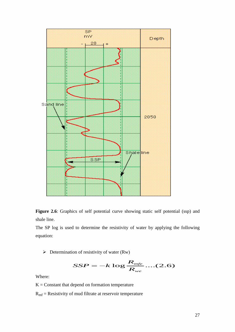
27

Figure 2.6: Graphics of self potential curve showing static self potential (ssp) and

shale line.

The SP log is used to determine the resistivity of water by applying the following

equation:

Determination of resistivity of water (Rw)

Where:

K = Constant that depend on formation temperature

Rmf = Resistivity of mud filtrate at reservoir temperature

)6.2....(logwe

mfe

R

RkSSP

28

Rwe = Equivalent resistivity of water

SSP= Static SP value.

The other uses of the SP log are the following:

Differentiate potentially porous and permeable reservoir rocks impermeable

clays

Define Bed Boundaries.

Give an indication of shaliness

2.4.2 Resistivity Logs

The Resistivity log is a measurement of the formation resistivity with direct current

using the principles of Ohm‟s law. The resistivity of a substance is a measure of its

ability to impede the flow of electric current .The basic measuring system has two

current electrodes and two voltage electrodes. Resistivity is the key to hydrocarbon

saturation determination and the measuring unit is ohm-meters and they are plotted on

a logarithm scales in track 2 or 3.

The Resistivity logs can be grouped into three measurements; Induction logs,

Laterologs, and Microresistivity measurements.

2.4.2.1 Induction Logs

The Induction logs measure the resistivity of the undisturbed part of the formation

laterally distant from the borehole .An induction tool uses a high frequency

electromagnetic transmitter to induce a current in a ground loop of formation. This in

turn induces an electric field whose magnitude is proportional to the formation

conductivity. Induction logs measure conductivity rather than resistivity.

The Induction tool is designed for an 8.5 inches hole and can be run successfully in

much larger hole sizes in which logging is usually performed with a 1.5 inch stand off

from the borehole wall. The tools work best in low resistivity formations and in Wells

drilled with high resistivity muds. Tool resolution is in the order of 6 feet. Depth of

investigation is 4 – 6 feet for the Medium Induction log (ILm) and about 10 feet for

the Deep Induction log (ILd).

The Typical applications of the Induction Logs are:

29

Measure the true(undisturbed) formation resistivity (Rt)

Ideal in Fresh or Oil -based environments

Ideal for Low resistivity measurements

Fluid saturation determination

2.4.2.2 Laterologs

The laterolog tools use focusing or bucking currents into a planar disc shape and

monitor the potential drop between an electrode on the tool and a distant electrode.

The potential drop changes as the current and the formation resistivity changes and

therefore the resistivity can be determined. Table 2.4 below present laterolog curves

display generic names commonly used.

Table 2.4: Curve names and mnemonics of laterolog

Curve Name Mnemonics

Deep Laterolog Resistivity DLL,LLD,RLLD

Shallow laterolog resistivity SLL,LLS,RLLS

(Krygowski, 2003)

The resolution of the tool is about 3-5 feet and depth of investigation of about 3 feet

for the LLs and 9-12 feet for the LLd.

Laterolog applications include the following:

Measures True(Undisturbed) formation resistivity Rt

Useful in medium to high resistivity environments

Overpressure detection

Fluid saturation determination

Diameter of invasion determination

Limitations of the Laterologs are:

Affected by the Groningen effects in some environments

Cannot be used in oil-based muds

Cannot be used in air-filled holes

30

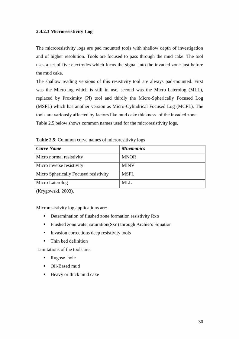
2.4.2.3 Microresistivity Log

The microresistivity logs are pad mounted tools with shallow depth of investigation

and of higher resolution. Tools are focused to pass through the mud cake. The tool

uses a set of five electrodes which focus the signal into the invaded zone just before

the mud cake.

The shallow reading versions of this resistivity tool are always pad-mounted. First

was the Micro-log which is still in use, second was the Micro-Laterolog (MLL),

replaced by Proximity (Pl) tool and thirdly the Micro-Spherically Focused Log

(MSFL) which has another version as Micro-Cylindrical Focused Log (MCFL). The

tools are variously affected by factors like mud cake thickness of the invaded zone.

Table 2.5 below shows common names used for the microresistivity logs.

Table 2.5: Common curve names of microresitivity logs

Curve Name Mnemonics

Micro normal resistivity MNOR

Micro inverse resistivity MINV

Micro Spherically Focused resistivity MSFL

Micro Laterolog MLL

(Krygowski, 2003).

Microresistivity log applications are:

Determination of flushed zone formation resistivity Rxo

Flushed zone water saturation(Sxo) through Archie‟s Equation

Invasion corrections deep resistivity tools

Thin bed definition

Limitations of the tools are:

Rugose hole

Oil-Based mud

Heavy or thick mud cake

31

2.5 AUXILIARY LOGS

These are logs that are required to assist in the quantitative interpretation of many

other logs that are sensitive to borehole diameter, wall roughness, hole deviation, and

fluid temperature. This includes; the calliper, temperature, and dipmeter logs.

2.5.1 Caliper Log

The calliper logs are the first runs in borehole to measure the diameter of the hole or

casing for corrections to other logs and measurements. The measurement of the

borehole diameter is done using two or four flexible arms, symmetrically placed on

each side of a logging tool.

The calliper shows where deviations occur from the nominal drill bit diameter. The

simple calliper log records the mechanical response of formations to drilling. Holes

with larger diameter than the bit size is caved or washed out. The curve is traditionally

a dashed line and usually plotted in track one with a scale of 6 to 16 inches. The log

also provides information on fracture identification, lithologic changes, well

construction and serve as input for environmental corrections for other measurements.

It can be run in any borehole conditions.

2.5.2 Temperature Log

The temperature tools measures the temperature of borehole fluids. Temperature

logging is used to detect changes in thermal conductivity of the rocks along the

borehole or to detect water flow through cracks or fractures.

The temperature log is normally plotted so that changes in the temperature gradient

(change in temperature to depth) might be related to lithological boundaries or

aquifers. Ideally the logging sonde is run twice; once immediately after drill rods are

withdrawn and after 24 hours in order to describe the temperature gradient.

The unit of measurement is normally in Degree Fahrenheit (oF). The logs are to be run

in fluid–filled boreholes and are also used for temperature corrections to other logs

and measurements.

32

2.5.3 Dipmeter Log

The dipmeter was the first structural logging tool (originally an SP dipmeter).The log

provides a continuous record of formation dip and direction of dip or azimuth. The

dipmeter measurements of borehole tilt and azimuth are based on magnetic and

gyroscopic sensors in the sonde. All recorded data are corrected to true dip and strike

and log is usually presented in a tadpole or arrow plot form with respect to true north

as presented in Figure 2.7.

Figure 2.7: Example of presentation of dip log

The log describes a correlation solution as tadpole with a prescribed frequency. Tool

rotation, magnetic field and gamma ray logs are included for quality control of the

log. Quality is dependent on low rotation frequency and calibration of the tool.

The dip angle is the angle formed between a normal to a bedding plane and vertical. A

horizontal bed has a dip angle of 0o and a vertical bed has a dip of 90

o.

The dip azimuth is the angle formed between the geographic north and the direction

of greatest slope on the bedding plane. Dip azimuth is conventionally measured

clockwise from north so that a plane dipping to east has a dip azimuth of 90o.

A group of dips of more or less constant low dip magnitude and more or less constant

azimuth is coloured green (Figure 2.7).Group of dips of more or less constant azimuth

33

showing an increase in dip magnitude with depth is coloured red, and that showing

decrease in dip magnitude with depth is coloured blue (Bateman, 1985). Depositional

features like sand bars and channels might be identified from the dipmeter plot.

2.6 OVERVIEW OF NEW GENERATION LOGGING TOOLS

The new generation of logging tools technology are developed to capture complete

map of the borehole wall in terms of diameter, deviation, light and colour. They have

higher resolutions. They can be divided into two categories:

Qualitative and quantitative devices.

The Qualitative devices include the following:

Dipmeter:

- Stratigraphical high Resolution Dipmeter tool (SHDT)

- Oil Base Dipmeter tool (OBDT)

Image Logs:

- Formation Micro-scanner (FMS) tool

- Full-bore Formation Micro-image (FMI) tool

- Borehole imaging in oil-base mud (OBMI)

- Borehole televiewer (BHTV)

- Azimuth Resistivity Imager (ARI)

- Array Induction Tool (AIT)

Quantitative Devices:

- Nuclear Magnetic Resonance (NMR)

- Combinable Magnetic Resonance (CMR)

- Pulsed Neutron Capture Log (PNC)

34

CHAPTER THREE

DESCRIPTION OF PETROPHYSICAL PROPERTIES

3.1 INTRODUCTION

Petrophysics is regarded as the study of rock and fluid systems. Petrophysical

measurements are made on cores in the laboratories and boreholes to determine the

major reservoir properties which include porosity, permeability, fluid saturations and

capillary pressure. The petrophysical parameters obtained from cores are used to

calibrate borehole measurements and for volume calculations. The petrophysical

parameters will be reviewed.

3.2 POROSITY

The porosity of a rock is the fraction of the total rock volume that can be filled with

gas, oil, water or a mixture of these fluids. The porosity developed in sedimentary

rocks is a function of the grain size distribution, grain shape, orientation and sorting.

When all the grains are of the same size, sorting is regarded as good and if grains of

diverse sizes are mixed together, sorting is regarded as poor.

The ratio of a volume of void spaces within a rock to the total bulk volume of that

rock is expressed as a percentage denoted as Φ. This is expressed mathematically as

Φ = Pore Volume * 100

Pore volume + Grain Volume

An example of pore space and grain space is given the Figure 3.1.

35

Figure 3.1: Example of pore space and mineral grain space.

There are many descriptions of porosity but the two common are the total and

effective porosities. The total porosity ΦT is defined as the ratio of total pore volume

within a rock to the total bulk volume including voids. The effective porosity Φe is

defined as the ratio of the interconnected pore space to the total bulk volume. The

Figure 3.2 below presents an example of effective, non-effective or isolated, and total

porosity of a rock.

36

Figure 3.2: Example of effective and total porosity.

The amount of porosity is mainly caused by the arrangement (cubic or rhombohedral),

size and sorting of rock. The cubic arrangement of grains has a maximum porosity of

about 48% and rhombohedral packing of maximum porosity of about 26% (Figure

3.3).

Sand Grain

Cementing material

Interconnected or Effective porosity

Isolated or Noneffective porosity

Total Porosity

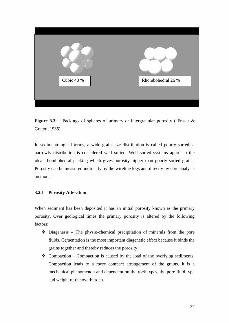
37

Figure 3.3: Packings of spheres of primary or intergranular porosity ( Fraser &

Graton, 1935).

In sedimentological terms, a wide grain size distribution is called poorly sorted; a

narrowly distribution is considered well sorted. Well sorted systems approach the

ideal rhombohedral packing which gives porosity higher than poorly sorted grains.

Porosity can be measured indirectly by the wireline logs and directly by core analysis

methods.

3.2.1 Porosity Alteration

When sediment has been deposited it has an initial porosity known as the primary

porosity. Over geological times the primary porosity is altered by the following

factors:

Diagenesis – The physio-chemical precipitation of minerals from the pore

fluids. Cementation is the most important diagenetic effect because it binds the

grains together and thereby reduces the porosity.

Compaction – Compaction is caused by the load of the overlying sediments.

Compaction leads to a more compact arrangement of the grains. It is a

mechanical phenomenon and dependent on the rock types, the pore fluid type

and weight of the overburden.

Cubic 48 % Rhombohedral 26 %

38

Leaching – Leaching occurs when minerals dissolve in the pore fluids. This

type of porosity is referred to as secondary porosity because it is produced

after deposition of the sediments.

Bioturbation – The mixing of deposited sediments caused by bioactivity of

small organisms such as worm that move through the sediments and leave a

trace of fine particles behind.

Clay coating – This involves crystals that grow on the surface of the grains

over geological times and can even completely fill pores (Schutjens, 1991).

3.3 PERMEABILITY

The permeability is the measure of the ease at which fluid flows through connecting

pore spaces of reservoir rock. The fluid flow is proportional to the gradient of

pressure. Permeability is controlled by size of pore openings, degree and size of pore

connectivity, type of cementing material between rock grains.

The concept of permeability originates from the laboratory flow tests carried out by

Henri Darcy in 1856. The following equation is an expression of Darcy‟s equation to

determine permeability.

K = Q μ / A (ΔP/L)..................................................... (3.1)

Where:

K = Permeability (darcy)

Q = Flow per unit time (cm/s)

μ=Viscosity of flowing medium (cp)

A = Cross section of rock (cm2)

L = Length of rock (cm)

ΔP = Change in pressure (psi)

The unit of measurement of permeability is in Darcies, more commonly in

millidarcies (md). A reservoir productive capacity is largely determined by its

permeability. Permeability is measured horizontally and vertically (Figure 3.4). The

39

horizontally measured permeability is accepted as the rock permeability because it is

measured parallel to the bedding which is the major contributor to fluid flow into a

typical reservoir. Vertical permeability (Kv) is usually less than horizontal

permeability (Kh) because of layering effects of sedimentation (Hughes, 2002).

Figure 3.4: Directions of measurement of permeability.

Three types of permeability are employed in Petroleum applications; absolute,

effective and relative .Permeability is absolute when the reservoir rock is completely

saturated with the flowing fluid. Permeability is effective to a particular fluid when

that fluid occupies less than 100 % of the pore space. An example is a gas or oil

permeability in a rock which contains connate water. Relative permeability is the ratio

of the effective to absolute permeability.

The permeability which could describe fluid flow in reservoirs is effective or relative

permeability. The values of permeability can be determined from Core analysis, well

tests, and drill stem test analysis. Permeability measured from core data is the most

accurate and values can be classified fair is permeability is between 1 to 10md; Good

from 10 to 100md; very good from 100 to 1000md. The Figure below present rock

permeability ranges (Garven, 1986).

Vertical Permeability Kv

Horizontal permeability Kh

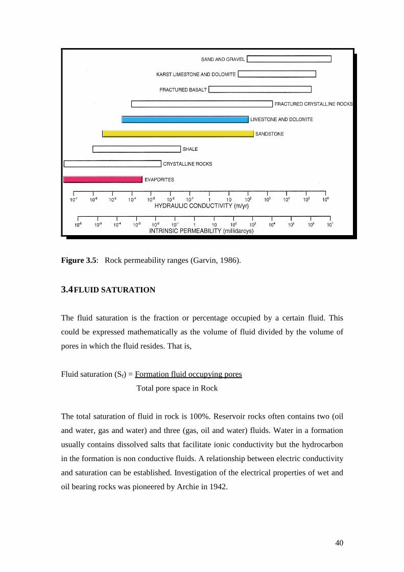
40

Figure 3.5: Rock permeability ranges (Garvin, 1986).

3.4 FLUID SATURATION

The fluid saturation is the fraction or percentage occupied by a certain fluid. This

could be expressed mathematically as the volume of fluid divided by the volume of

pores in which the fluid resides. That is,

Fluid saturation (Sf) = Formation fluid occupying pores

Total pore space in Rock

The total saturation of fluid in rock is 100%. Reservoir rocks often contains two (oil

and water, gas and water) and three (gas, oil and water) fluids. Water in a formation

usually contains dissolved salts that facilitate ionic conductivity but the hydrocarbon

in the formation is non conductive fluids. A relationship between electric conductivity

and saturation can be established. Investigation of the electrical properties of wet and

oil bearing rocks was pioneered by Archie in 1942.

41

3.4.1 Electrical Formation Water

The method Archie used to arrive at the conclusion of his investigation on resistivity

and saturation was simple. He took a number of cores of different porosity and

saturated each one with a variety of brines. He measured the resistivity of the water

Rw and the resistivity of the 100% water saturated rock Ro. When the results were

plotted, he found a series of straight lines of slope F referred to as the electrical

formation factor (Bateman, 1985).

The rock formation factor is the resistivity of a rock sample completely saturated with

water to the resistivity of the water. Mathematically; it can be expressed as follows:

F = Ro............................ (3.2)

Rw

Where:

Ro = Resistivity of 100 % saturated rock (Ohm-m)

Rw = Resistivity of water (Ohm-m)

Archie found out that measured value of F could be related to the porosity of the rock

by an equation of the form

F = 1

Φm

Where:

Φ = Porosity

m=cementation exponent

Another empirical equation relating F and Φ was also suggested by the results of

experiment measurements conducted by Winsauer et al (Bassouni, 1994). The

equation is of the form

F =a........................................ (3.3)

Φm

Where:

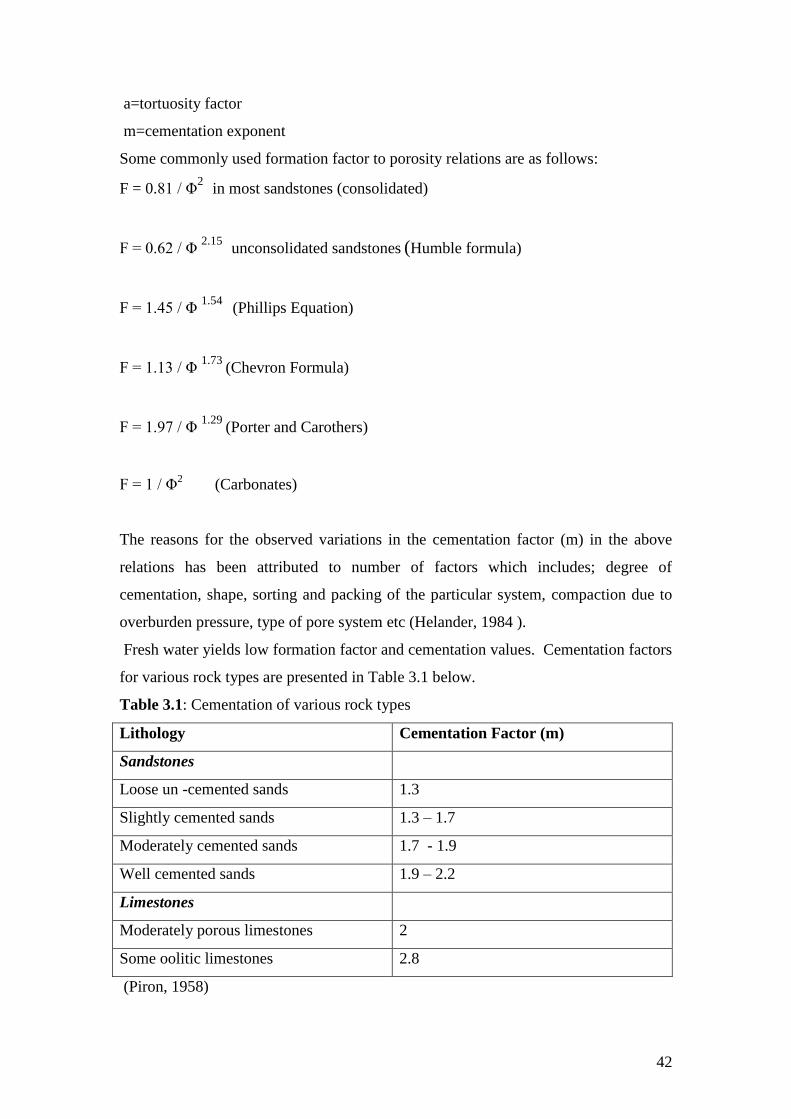
42

a=tortuosity factor

m=cementation exponent

Some commonly used formation factor to porosity relations are as follows:

F = 0.81 / Φ2

in most sandstones (consolidated)

F = 0.62 / Φ 2.15

unconsolidated sandstones (Humble formula)

F = 1.45 / Φ 1.54

(Phillips Equation)

F = 1.13 / Φ 1.73

(Chevron Formula)

F = 1.97 / Φ 1.29

(Porter and Carothers)

F = 1 / Φ2

(Carbonates)

The reasons for the observed variations in the cementation factor (m) in the above

relations has been attributed to number of factors which includes; degree of

cementation, shape, sorting and packing of the particular system, compaction due to

overburden pressure, type of pore system etc (Helander, 1984 ).

Fresh water yields low formation factor and cementation values. Cementation factors

for various rock types are presented in Table 3.1 below.

Table 3.1: Cementation of various rock types

Lithology Cementation Factor (m)

Sandstones

Loose un -cemented sands 1.3

Slightly cemented sands 1.3 – 1.7

Moderately cemented sands 1.7 - 1.9

Well cemented sands 1.9 – 2.2

Limestones

Moderately porous limestones 2

Some oolitic limestones 2.8

(Piron, 1958)

43

w

n

S a

m

Rw

Rt

3.4.2 Water Saturation (Sw)

Archie experiment showed that water saturation could be related to its resistivity. He

defined the resistivity index IR as the ratio of the resistivity of a partially water

saturated rock Rt to the resistivity of the fully brine saturated rock Ro.

IR = Rt ............................................ (3.4a)

Ro

If the rock sample was originally fully saturated with water, then Rt will equal Ro and

IR will equal one. The presence of hydrocarbon is indicated by the value of the

resistivity index. Saturation can be expressed as a ratio of the resistivities:

………………………………(3.4b)

Where n is the saturation exponent an empirical constant and taken as two in most

case. Substituting for Ro in equation 3.4a and F in equation 3.4b above, the

expression the water saturation becomes

The Archie‟s equation links the porosity and resistivity with the amount of water

present Sw in the formation. Increasing porosity will reduce the water saturation for

the same Rt. Once the water saturation is known; the hydrocarbon saturation can be

calculated.

SHC = 1 – Sw

Where:

SHC = Hydrocarbon saturation.

Sw = Water Saturation.

t

n

wR

RS 0

44

The Archie‟s model considers the electrolytes in the pores as the only conductive

path, hence the relationship is valid for only clean sand formations. Shaly sand

formations exhibit more complex behaviour because clay minerals present in the

formation contribute an additional pararell conductive path in addition to the

formation salinity.

3.4.3 Influence of Clay on rock resistivity

The presence of clay in a rock will influence the resistivity of the rock depending on

the type and distribution of the clay. The presence of cation exchangeable clays often

cause apparent low resistivity index values to be observed which also causes a

decrease in water saturation calculations. The conductivity of the clay is related to the

cation exchange capacity (CEC).The higher the CEC, the lower the formation factor

at any salinity.

Active sites exist on clay surfaces where cations may be exchanged with drilling mud

fluid. This ion exchange may alter formation porosity, reduce permeability, formation

resistivity and also result in erroneous high calculation of water saturations from

downhole logs. Waxman-Smit-Thomas and other researchers proposed equations that

allow calculations of a formation factor independent of the clay conductivity effects

(Core laboratories, 1982).

3.5 CAPILLARY PRESSURE

Capillary pressure reflects the interaction of rock and fluids and is controlled by the

pore geometry, interfacial tension and wettability. Hydrocarbon reservoirs can be

regarded as a capillary system where in the absence of other forces, the distribution of

the fluids is determined by the interaction of gravity, interfacial tension and

wettability.

The wettability is defined as the contact angle between droplets of liquid on a

horizontal surface. It is a measure of which fluid adheres to the rock. The wettability

describes the affinity between a liquid and a solid. The fluid/fluid interaction

dominated by intermolecular van der Waal forces is regarded as the interfacial

tension. The gravity plays a role in both wettability and interfacial tension situations.

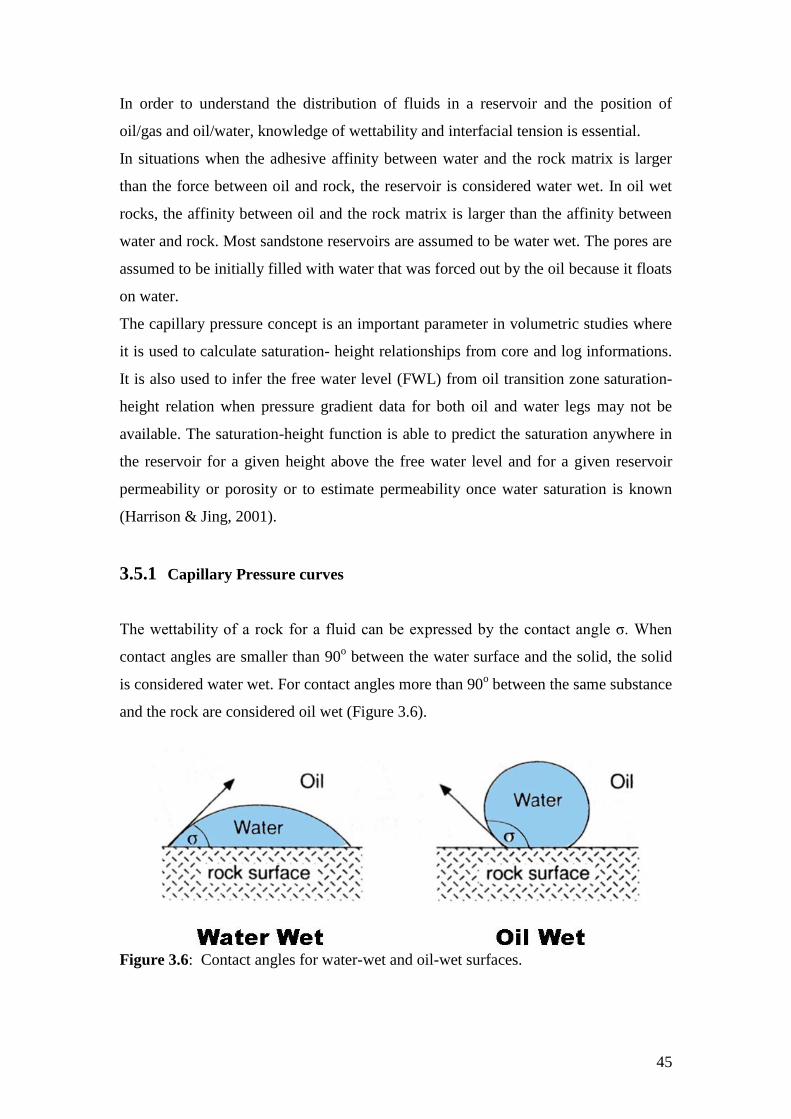
45

In order to understand the distribution of fluids in a reservoir and the position of

oil/gas and oil/water, knowledge of wettability and interfacial tension is essential.

In situations when the adhesive affinity between water and the rock matrix is larger

than the force between oil and rock, the reservoir is considered water wet. In oil wet

rocks, the affinity between oil and the rock matrix is larger than the affinity between

water and rock. Most sandstone reservoirs are assumed to be water wet. The pores are

assumed to be initially filled with water that was forced out by the oil because it floats

on water.

The capillary pressure concept is an important parameter in volumetric studies where

it is used to calculate saturation- height relationships from core and log informations.

It is also used to infer the free water level (FWL) from oil transition zone saturation-

height relation when pressure gradient data for both oil and water legs may not be

available. The saturation-height function is able to predict the saturation anywhere in

the reservoir for a given height above the free water level and for a given reservoir

permeability or porosity or to estimate permeability once water saturation is known

(Harrison & Jing, 2001).

3.5.1 Capillary Pressure curves

The wettability of a rock for a fluid can be expressed by the contact angle σ. When

contact angles are smaller than 90o between the water surface and the solid, the solid

is considered water wet. For contact angles more than 90o between the same substance

and the rock are considered oil wet (Figure 3.6).

Figure 3.6: Contact angles for water-wet and oil-wet surfaces.

46

In capillary pressure measurements, a non wetting fluid invades the pore system that

was originally occupied by a wetting fluid whereby the latter is displaced by the

former. The capillary pressure of a non wetting fluid invading into the pores is

described by Laplace‟s equation (Dullien, 1979) as follows:

Pc = 2 γ = 2γ cosσ................................. (3.5)

R pore R pore

Where:

Pc = Capillary pressure

γ=interfacial tension

R = Average radius of pores

σ =contact angle

The Laplace equation (3.5) describes the relationship between the radius of the pore

and the pressure that is required for the fluid to enter the pore. The laboratory values

of capillary pressure can be converted to equivalent reservoir condition values as

follows:

Pc (res) = Pc (lab) (γ cosσ)res ........................(3.6)

(γ cosσ)lab

Typical values for interfacial tension and contact angles taken from core laboratory

manual are given in Table 3.2. The laboratory to reservoir condition conversion

considers the difference in capillary pressure due to interfacial tension and contact

angle. The interfacial angle can be measured at laboratory and reservoir conditions but

the contact angle is difficult to measure especially for systems that are not strongly

wet.

47

Table 3.2: Interfacial tension and contact angle values

Wetting

Phase

Non-Wetting

Phase

Conditions:

Température(T)

Pressure(P)

Contact

Angle(σ)

Interfacial

Tension

(dynes/cm)

Brine Oil Reservoir,T,P 30 30

Brine Oil Laboratory,T,P 30 48

Brine Gas Laboratory,T,P 0 72

Brine Gas Reservoir,T,P 0 50

Oil Gas Reservoir,T,P 0 4

Gas Mercury Laboratory,T,P 140 480

(Core Laboratories, 1982)

Reservoir water saturation decreases with increasing height above the free water level

where capillary pressure is zero. A minimum water saturation (Swirr) is reached at a

great height above the free water level and this water saturation is immobile. The

transition zone is defined as the zone which can produce both hydrocarbon and water.

Changes in the capillary pressure radius are controlled by the pore geometry which is

a function of rock properties such as permeability and porosity. The pore size

distribution also has a great influence on the magnitude of the irreducible water

saturation (Swirr) and height of the transition zone. The hydrocarbon water contact

will vary with depth as a function of the reservoir quality. The higher the

permeability, the smaller the separation between oil water contact and free water level

(Harrison & Jing, 2001).

3.5.2 Capillary pressure and seal

The seal is a rock which prevents natural buoyancy related upward migration of

hydrocarbon. Hunt (1990) extended the definition to any rock which is capable of

preventing all pore fluid movement over a substantial period. A seal is controlled by

the largest flaw in the sealing rock generally near the crest. The weakness of the seal

can be due to diagenesis and tectonic force. For a hydrocarbon to be trap, the upward

buoyancy must be smaller than the downward capillary pressure.

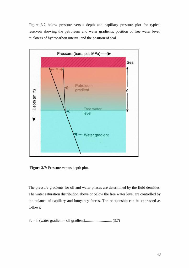
48

Figure 3.7 below pressure versus depth and capillary pressure plot for typical

reservoir showing the petroleum and water gradients, position of free water level,

thickness of hydrocarbon interval and the position of seal.

Figure 3.7: Pressure versus depth plot.

The pressure gradients for oil and water phases are determined by the fluid densities.

The water saturation distribution above or below the free water level are controlled by

the balance of capillary and buoyancy forces. The relationship can be expressed as

follows:

Pc = h (water gradient – oil gradient)............................ (3.7)

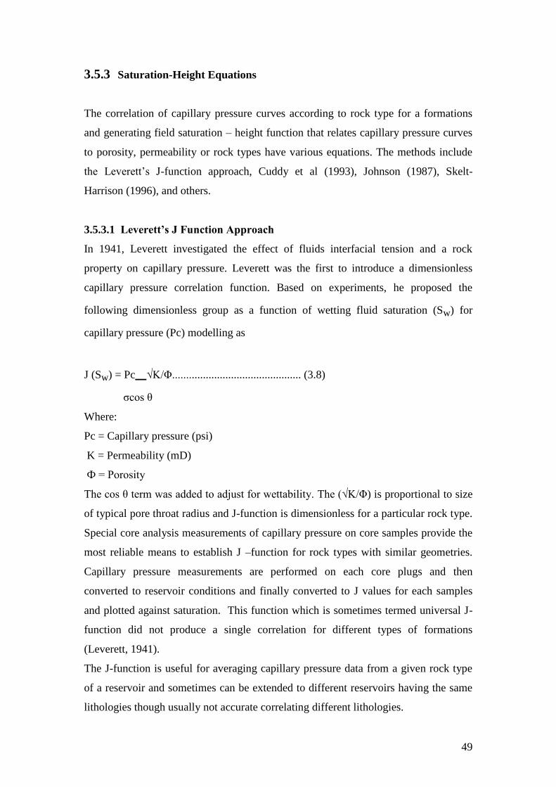
49

3.5.3 Saturation-Height Equations

The correlation of capillary pressure curves according to rock type for a formations

and generating field saturation – height function that relates capillary pressure curves

to porosity, permeability or rock types have various equations. The methods include

the Leverett‟s J-function approach, Cuddy et al (1993), Johnson (1987), Skelt-

Harrison (1996), and others.

3.5.3.1 Leverett’s J Function Approach

In 1941, Leverett investigated the effect of fluids interfacial tension and a rock

property on capillary pressure. Leverett was the first to introduce a dimensionless

capillary pressure correlation function. Based on experiments, he proposed the

following dimensionless group as a function of wetting fluid saturation (Sw) for

capillary pressure (Pc) modelling as

J (Sw) = Pc √K/Φ.............................................. (3.8)

σcos θ

Where:

Pc = Capillary pressure (psi)

K = Permeability (mD)

Ф = Porosity

The cos θ term was added to adjust for wettability. The (√K/Φ) is proportional to size

of typical pore throat radius and J-function is dimensionless for a particular rock type.

Special core analysis measurements of capillary pressure on core samples provide the

most reliable means to establish J –function for rock types with similar geometries.

Capillary pressure measurements are performed on each core plugs and then

converted to reservoir conditions and finally converted to J values for each samples

and plotted against saturation. This function which is sometimes termed universal J-

function did not produce a single correlation for different types of formations

(Leverett, 1941).

The J-function is useful for averaging capillary pressure data from a given rock type

of a reservoir and sometimes can be extended to different reservoirs having the same

lithologies though usually not accurate correlating different lithologies.

50

3.5.3.2 Johnson Capillary method

Johnson (1987) proposed another way of correlating capillary pressure data water

saturation to permeability. Using special core analysis data, Johnson observed that the

plots of water saturation versus permeability for each capillary pressure de-saturation

step were approximate straight and parallel lines when drawn on log/log axes. His

permeability averaging method gives an empirical function that relates capillary

pressure to water saturation and permeability as follows:

Log (Sw) = B. Pc-c

–A.log(K) ..............................................(3.9)

Where:

A, B, and C = Constant

Sw = Water saturation (percent)


Pc = Capillary Pressure (psi)

The constants A, B and C are derived from special core analysis measurements

capillary pressure data using series of cross plots. Johnson states that his method is not

universal but it has proved effective in some North Sea reservoirs (Johnson, 1987).

3.5.3.3 Skelt-Harrison Capillary Pressure and log Based Method

Skelt recommends the fitting of a curve to a set of height and saturation data. It was

initially to the capillary pressure data from special core analysis measurements and

then refines this to fit the log derived water saturation data. Each data point was

assigned a different weight during the regression (Skelt & Harrison, 1995).

The strength of the Skelt‟s function is that rather than linearise the function using

logarithms, it makes use of its non-linearity to provide a fitted curve shape that

actually looks like a capillary pressure curve. The equation is of the form:

Sw = 1 – A exp. [-(B / h +D )c ] ..........................................(3.10)

Where:

A, B, C and D = Coefficients found by regression to core and log data. h=Height

above free water level

51

CHAPTER FOUR

WIRELINE LOG EDITING AND NORMALIZATION

4.1 INTRODUCTION

The aim of wireline logging is to measure and record a given formation‟s properties in

its undisturbed state and convert it to petrophysical parameter. The objective is rarely

achieved because the drilled hole where the logging operation is performed is not

perfect and the logging environment also is often affected by drilling mud type, mud

salinity, that need to be removed in order to get the actual response of the logs.

When raw log data are collected for formation evaluations it is essential to check the

quality of the data and perform editing if necessary before performing quantitative

interpretation. Log editing is basically a form of log interpretation aimed at removing

or correcting problems that affect logs and provides the best possible presentation of

the in-situ properties measured and recorded by logs. Some of the problems

encountered by logs that need to be edited before using it for quantitative

interpretations are the following:

Depth Shifting/Matching

Borehole environmental corrections

Smoothing/De-spiking/Noise Removal

Merging/splicing of curves

After performing the editing process, the next stage is curves normalization.

Normalization is a mathematical process that adjusts for differences among data from

varying sources in order to create a common basis for comparison.

The flow chart starting from data collection through the editing processes to

quantitative analysis is given in Figure 4.1 below. However, this chapter starts with

the process of wireline log data collection and end on log normalization of the ten

wells within the study area.

52

Figure 4.1: Flow chart of Log editing.

Very Good

53

4.2 LOG DATA COLLECTION AND CREATION OF DATABASE

A conventional suite of open –hole wireline log data were run by Schlumberger in all

the vertical exploration wells drilled between 1987 and 2003 and logged by

Schlumberger wireline Company. Water based mud (WBM) were used to drill wells

MA1 ,MA2, MA3, MA4, OP1, and OP3, while oil based mud (OBM) were used to

drill wells (OP2, OP4, OP5 and OP6).

All the wells were logged with basic log data suites and the data were provided by

Petroleum agency of South Africa (PASA) and PetroSA in Log ASCII format (LAS),

comprising measurements of:

Gamma- Ray, Caliper, Spontaneous Potential

Porosity – Density, Neutron, and Sonic

Resistivity Logs

-Water Based Mud wells – Dual laterolog, MSFL.

-Oil Based mud wells – Dual Induction

Digital data were provided in LAS format files at different Runs across the wells. The

logs were loaded into Interactive Petrophysics software created database. The log

header information and well completion report provides information on the interval of

wireline log for wells as given in the next subsection below. The logging suite tool

code name and description are shown in appendix A.

4.2.1 Wireline logged Intervals for Wells

The objectives of the well drilling project were to drill, log and test the primary target

intervals in order to prove a commercially viable gas reserve. Schlumberger Company

provided the wireline data with overall log quality very good. A suite of wireline logs

were available and successful Runs were conducted with well problems limited to

minor tight hole conditions at various intervals but were remedied by washing and

reaming during wiper trips. The static bottom hole temperature was estimated using

the Dowdle and Cobb method.

54

The Table 4.1 presents the suite of wireline logs available and successful Runs

conducted at different intervals as indicated in the Table 4.1 below.

Table 4.1: Suite of Logs Run in wells at various intervals

Well Run

Number

Hole size (in) Interval (m) Logging Suite

MA1 1 12 1/4 1118 - 240.6 HALS/ DSI/ TLD/ MCFL/ PEX.

2 8 1/2 3309.4 - 1107 HALS/DSI/TLD/MCFL/PEX

MA2 1 12 1/4 1114 - 280.4 HALS/DSI/TLD/MCFL

2 8 1/2 3171 - 1117 HALS/DSI/TLD/MCFL

MA3 1 12 1/4 1118 - 240.6 HALS/ DSI/ TLD/ MCFL/ PEX.

2 8 1/2 3309.4- 1107 HALS/DSI/TLD/MCFL/PEX

MA4 1 12 1/4 1134.9 - 256 HALS/ DSI/ TLD/ MCFL/ PEX.

2 8 1/2 3487.74 - 1090 HALS/DSI/TLD/MCFL/PEX

OP1 1 12 1/4 1781 - 3010 ISF-MSFL-BHC-SP-GR, LDT-CNL-

GR,SHDT-GR

2 8 1/2 3020 - 3520 MSFL-ILD-BHC-GR-SP,LDT-

CNL,SHDT,VSP

3 8 1/2 3552 - 3071 ISF-MSFL-ILD-BHC-GR

OP2 1 8 1/2 1256.7 - 3520 DIL/LDT/CNL/Sonic/GR

OP3 1 12 1/4 1386 - 3115 ISF-MSFL-SP-BHC-GR,LDT-

CNL,SHDT

2 8 1/2 3107 - 3681 ISF-MSFL-SP-BHC-GR;LDT-

CNL;SHDT

OP4 1 8 1/2 1575 - 3430 AIT/LDT/CNL/DSI/GR

OP5 1 8 1/2 772.5 - 3463 SP-AIT-NGT-DSI-PEX

OP6 1 8 1/2 1750 - 3412 AIT/LDT/CNL/DSI/GR

55

4.3 LOG EDITING

4.3.1 Depth Shifting

When combining measurements made during separate log runs through the same

borehole, discrepancies often arise and it is important that the measurements be

correctly correlated in depth with one another before performing quantitative

interpretation. Logs from different wireline tool strings may have slight mismatches

that may exist because of ship heave during recording, cable stretch, tidal changes in

sea level etc (Hagelberg et al., 1992). A curve is chosen e.g. natural gamma-ray log or

resistivity as a reference curve that provide means of depth shifting for correlation

with other curves and appropriate adjustments or shifts are applied.

For this study, the Interactive Petrophysics (IP) triple combination (triple combo)

module was applied for depth checking and was confirmed that no depth matching

was required except for wells that have core data that need to be depth matched with

the log data. Figure 4.2 below present example of curve run in all track with the

gamma ray log to check corresponding depth.

Figure 4.2: Example of gamma-ray log Run at the same depth with other logs.

OP1Scale : 1 : 100

DEPTH (3364.M - 3379.2M) 2009/12/03 09:24DB : Petrophysical Ihbubesi (14)

1

DEPTH

(M)

2

CALI (IN)6. 16.

Run2:GR (GAPI)0. 150.

6


Run2:ILD (OHMM)0.2 2000.

7


DT (US/F)140. 40.

8


RHOC (G/C3)1.95 2.95

3375

3370

Shale

Shale

Clean

Sand

56

The Figure above shows gamma –ray log (green colour) in track 2 and resistivity (red)

in track 6, sonic log (Foschini ) in track 7, and density log (red) in track 8 both

recorded at the same depth and Run, while the gamma-ray log is used to check if they

all record the same formation at a given depth. The gamma-ray or resistivity log could

be used as the reference shift curve.

No depth shift was required except for well that have core data that was depth shifted

with logs.

4.3.2 Borehole environmental correction

Logs are affected by borehole size and the environment, thus environmental

corrections by computer programs are applied. Borehole environmental influence is

caused by stress, mud weight, temperature, etc. All pad type devices such as the

density, sidewall neutron log, microlog, and dipmeter will not perform effectively in

large holes where the hole diameter is beyond the reach of the pad. The tools will read

the mud values or jump from high to low values due to the intermittent contact with

the borehole wall (Crain, 2001).Rough or rugose holes and shale intervals due to

washout will also leave excessive mud between the pad and the borehole wall and can

be observed from the Caliper and density correction DRHO logs as it will be very

high in such intervals.

Borehole environmental corrections have been applied to the following logs using

mud/borehole properties identified from log headers as presented in Table 4.2 below.

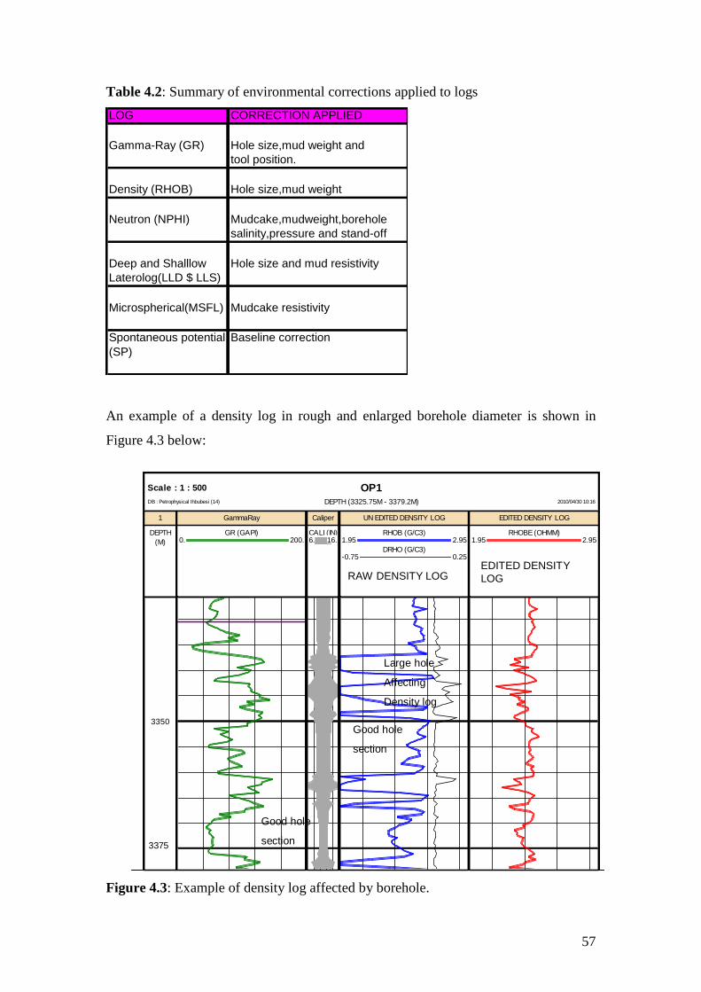
57

Table 4.2: Summary of environmental corrections applied to logs

LOG CORRECTION APPLIED

Gamma-Ray (GR) Hole size,mud weight and

tool position.

Density (RHOB) Hole size,mud weight

Neutron (NPHI) Mudcake,mudweight,borehole

salinity,pressure and stand-off

Deep and Shalllow Hole size and mud resistivity

Laterolog(LLD $ LLS)

Microspherical(MSFL) Mudcake resistivity

Spontaneous potential Baseline correction

(SP)

An example of a density log in rough and enlarged borehole diameter is shown in

Figure 4.3 below:

Figure 4.3: Example of density log affected by borehole.

OP1Scale : 1 : 500

DEPTH (3325.75M - 3379.2M) 2010/04/30 10:16DB : Petrophysical Ihbubesi (14)

1

DEPTH

(M)

GammaRay

GR (GAPI)0. 200.

Caliper

CALI (IN)6. 16.

UN EDITED DENSITY LOG

RHOB (G/C3)1.95 2.95

DRHO (G/C3)-0.75 0.25

EDITED DENSITY LOG

RHOBE (OHMM)1.95 2.95

3350Good hole

section

Large hole

Affecting

Density log

EDITED DENSITY

LOGRAW DENSITY LOG

Good hole

section3375

58

The Table 4.3 below presents guide as to know when to apply corrections due to

borehole condition (Yan et al., 2008).

Table 4.3: Guide for borehole condition

Caliper and Bit size(BS) logs Condition

Caliper – BS = 0 % Excellent condition, no need for correction

Caliper – BS < 10 % Logs are good quality, refer to DRHO log

Caliper – BS =10 – 30% Logs probably need to be corrected

Caliper –BS >30 – 50% Logs incorrect, need to correct

Caliper – BS > 50 % Very bad borehole conditions. incorrect logs

(Yan et al., 2008)

The use of service company chart books provide options for environmental

corrections and the input parameters includes raw log data, tool type, caliper log,

drilling bit size (BS), and mud information.

The mud properties used were taken from log data files and Well completion reports.

Hole size was taken from recorded bit size and Caliper log.

Figure 4.4 below presents an example of an uncorrected log and environmentally

corrected logs. Green colour curves with C appended to the suffixes are corrected

curves, while Red coloured curves are the uncorrected curves. After performing the

corrections, the curves tend to increase in values except the resistivity logs as

presented in the Figure.

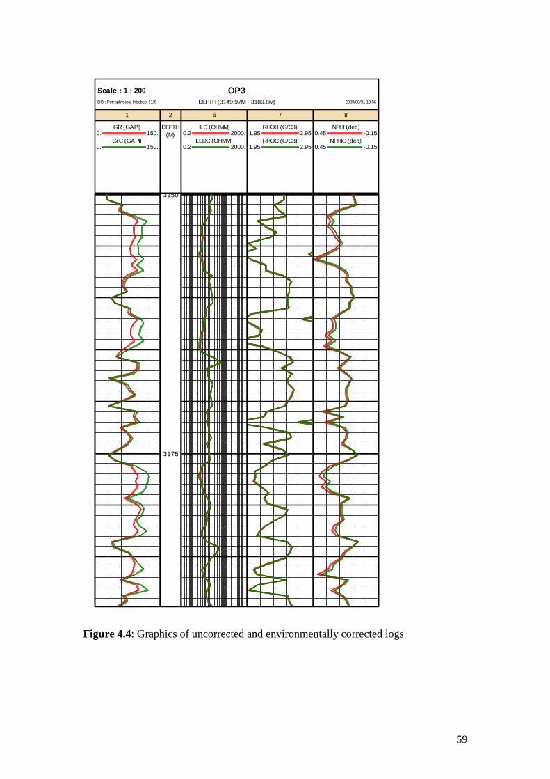
59

OP3Scale : 1 : 200


1

GR (GAPI)0. 150.

GrC (GAPI)0. 150.

2

DEPTH

(M)

6

ILD (OHMM)0.2 2000.

LLDC (OHMM)0.2 2000.

7

RHOB (G/C3)1.95 2.95

RHOC (G/C3)1.95 2.95

8

NPHI (dec)0.45 -0.15

NPHIC (dec)0.45 -0.15

3150

3175

Figure 4.4: Graphics of uncorrected and environmentally corrected logs

60

4.3.3 Mud filtrate Invasion Correction

The sonic, shallow resistivity and density logs have shallow depths of investigations

and their measured values comes from the near the wellbore so are all affected by

invasion. The mud filtrate invasion into the borehole can be up to 0.5m to 0.8m when

using water based mud in the drilling process. Studies by Chi et al (2004) showed that

the maximum invaded distance is about 2m therefore if the invasion depth is beyond

the depth of the investigation of the logging tool; it will result in tool showing values

from the invaded zone.

The conductive mud used in drilling also causes the induction log to read too low

values due to invasion and invasion correction charts could be used in such cases. The

correction for a fresh mud in a hydrocarbon zone will reduce resistivity values instead

of increasing it. The resistivity logs can be used to identify invasion zones.

Presented in Figure 4.5 is an example of the use of the resistivity log for recognition

of thin bed.

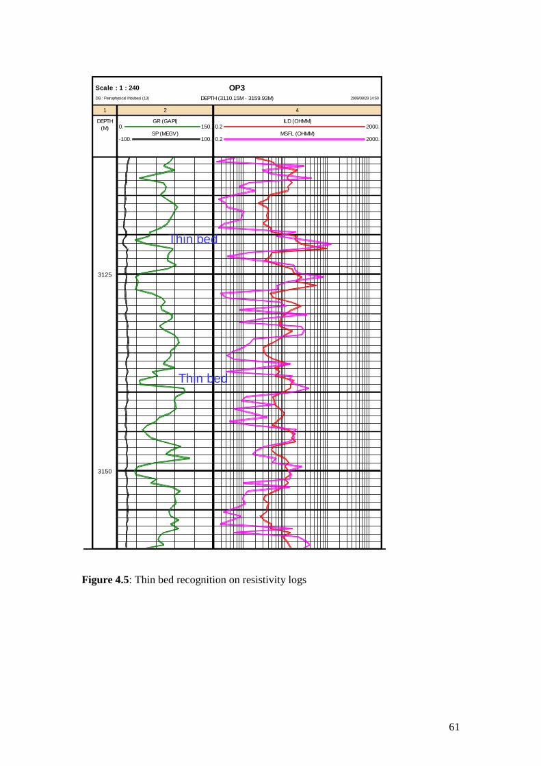
61

Figure 4.5: Thin bed recognition on resistivity logs

OP3Scale : 1 : 240


1

DEPTH

(M)

2

GR (GAPI)0. 150.

SP (MEGV)-100. 100.

4

ILD (OHMM)0.2 2000.

MSFL (OHMM)0.2 2000.

3125

3150

Thin bed

Thin bed

62

4.3.4 Smoothing, De-Spiking and Noise Removal

The process of de-spiking is an editing that involves removing of unwanted signals in

form of cycle skip, noise and spike that is associated with sonic logs. Care must be

taken in editing noise because some of the noise may be as a result of thinly bedded

porous layers. Track 6 in Figure 4.6 below present a sonic log data with spike. On

Track 9 is the edited sonic log without spike. When spikes are removed, the quality of

the sonic log data is improved (track 9).

OP2Scale : 1 : 500


2

DEPTH

(M)

5

GRn (GAPI)0. 150.

9

DTCO_E (US/FT)140. 40.

6

DT (US/F)140. 40.

3300

3350

Figure 4.6: Example of spike and de-spiking of sonic log

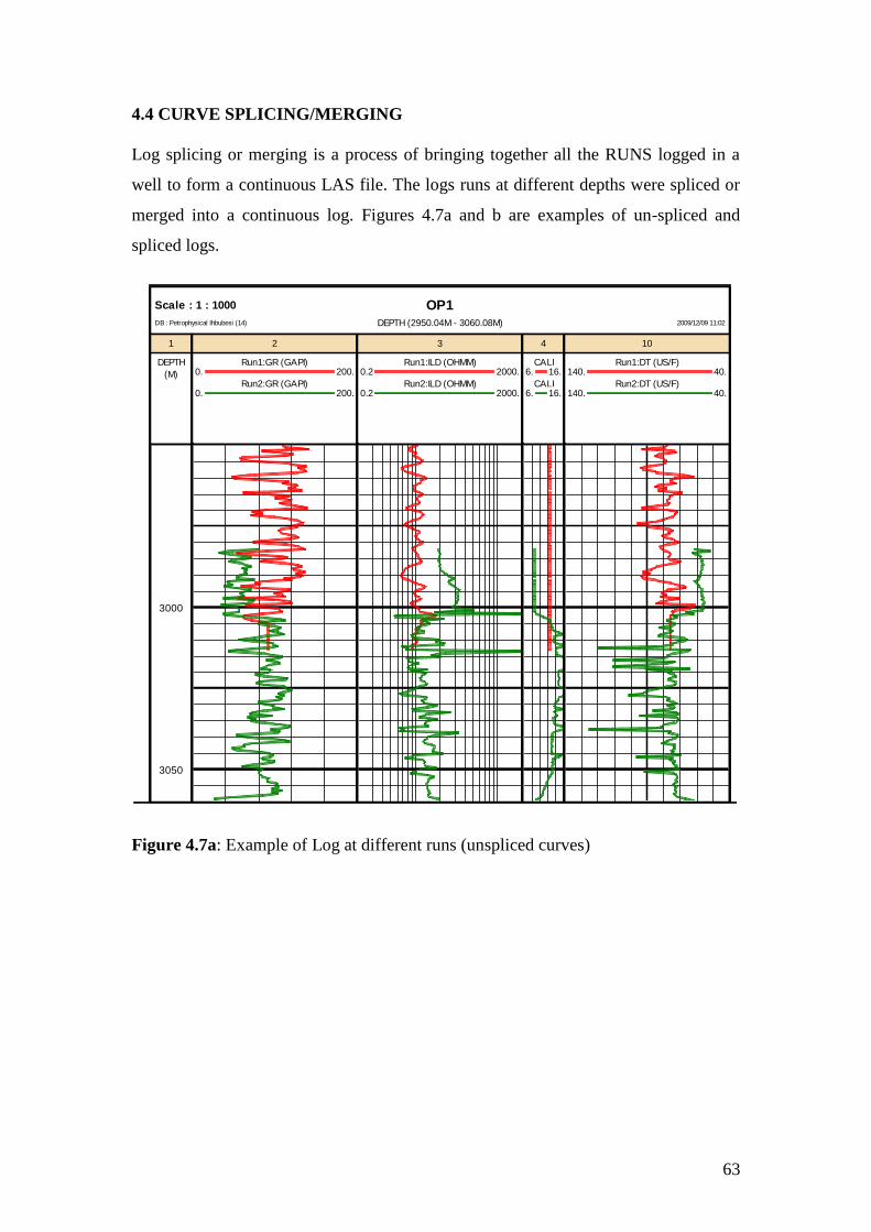
63

4.4 CURVE SPLICING/MERGING

Log splicing or merging is a process of bringing together all the RUNS logged in a

well to form a continuous LAS file. The logs runs at different depths were spliced or

merged into a continuous log. Figures 4.7a and b are examples of un-spliced and

spliced logs.

OP1Scale : 1 : 1000


1

DEPTH

(M)

2



3



4

CALI6. 16.

CALI6. 16.

10

Run1:DT (US/F)140. 40.

Run2:DT (US/F)140. 40.

3000

3050

Figure 4.7a: Example of Log at different runs (unspliced curves)

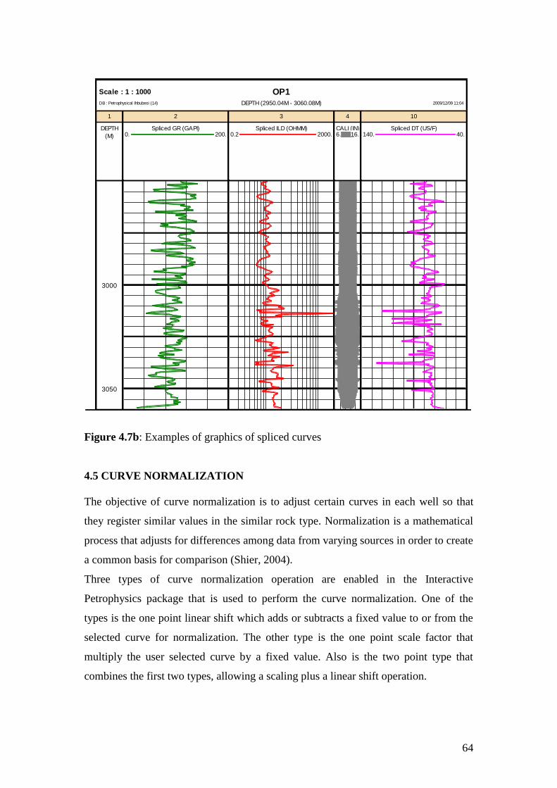
64

OP1Scale : 1 : 1000


1

DEPTH

(M)

2

Spliced GR (GAPI)0. 200.

3

Spliced ILD (OHMM)0.2 2000.

4

CALI (IN)6. 16.

10

Spliced DT (US/F)140. 40.

3000

3050

Figure 4.7b: Examples of graphics of spliced curves

4.5 CURVE NORMALIZATION

The objective of curve normalization is to adjust certain curves in each well so that

they register similar values in the similar rock type. Normalization is a mathematical

process that adjusts for differences among data from varying sources in order to create

a common basis for comparison (Shier, 2004).

Three types of curve normalization operation are enabled in the Interactive

Petrophysics package that is used to perform the curve normalization. One of the

types is the one point linear shift which adds or subtracts a fixed value to or from the

selected curve for normalization. The other type is the one point scale factor that

multiply the user selected curve by a fixed value. Also is the two point type that

combines the first two types, allowing a scaling plus a linear shift operation.

65

Well log normalization especially the gamma-log is useful for multi-well

characterisation of facie types, assessing the lateral continuity of reservoir sands,

geological analysis and mapping and determining net pay (Scott et al., 2004).

The first step in the log normalization was the histogram plot of GR values of all the

wells over the intervals and compared as shown in Figure 4.8a below.

Figure 4.8a: GR log values for all Well before Normalization.

The second step in the normalization process is to choose a standard or reference well

whose histogram is very similar and its geographical location is central to other wells.

In this case, well OP4 and OP5 were chosen as the reference wells and histogram

distributions are given in Figure 4.8b .

All Well

GR Curve distributions Before Normalization

0

20

40

60

80

100

Cu

mu

lativ

e F

req

ue

nc

y

0. 300.

0

50

100

150

200

250

300

350

400

Nu

mb

er

of

Po

ints

All Well

GR Curve distributions Before Normalization

0

20

40

60

80

100

Cu

mu

lativ

e F

req

ue

nc

y

0. 300.

0

200

400

600

800

1000

1200

Nu

mb

er

of

Po

ints

66

Figure 4.8b: Possible Reference wells (OP4 and OP5) used for Normalization

The next step in the process is to carry out the normalization process. Because all the

wells were logged by the same Company (Schlumberger), the range of the gamma-ray

log responses were similar and the normalization required was a simple shift .The two

point type of normalization was adopted in this study which is of the form given

below:

GRn = Input GR curve * x + C

Where:

GRn = Normalized curve

X = Factor to be multiplied with input curve

C = Value to be added to curve.

The normalized curves have n appended to the curve mnemonic and are presented in

Figure 4.8c below.

Well OP4 and OP5 Used for Normalization

Possible Reference wells

0

20

40

60

80

100

Cu

mu

lativ

e F

req

ue

nc

y

0. 300.

0

50

100

150

200

250

300

350

400

Nu

mb

er

of

Po

ints

Well OP4 and OP5 Used for Normalization

Possible Reference wells

0

20

40

60

80

100

Cu

mu

lativ

e F

req

ue

nc

y

0. 300.

0

100

200

300

400

500

Nu

mb

er

of

Po

ints OP4

OP5

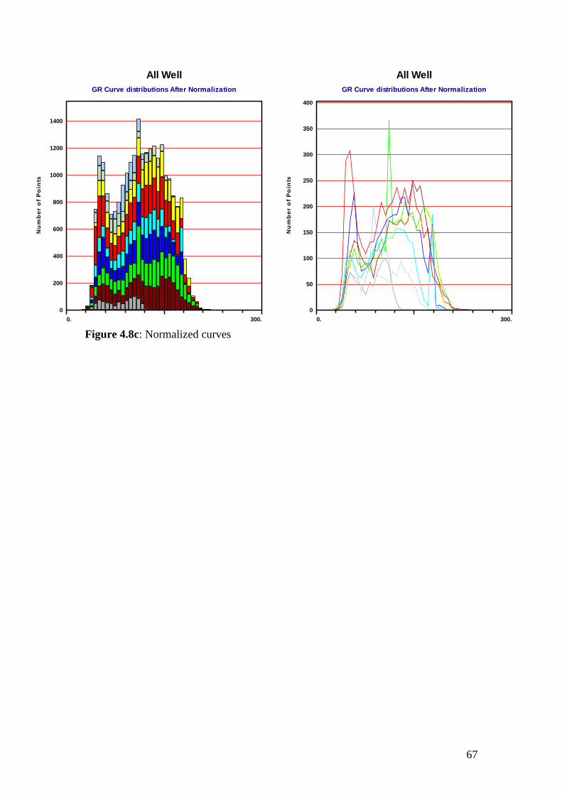
67

Figure 4.8c: Normalized curves

All Well

GR Curve distributions After Normalization

0

50

100

150

200

250

300

350

400

Nu

mb

er

of

Po

ints

0. 300.

All Well

GR Curve distributions After Normalization

0

200

400

600

800

1000

1200

1400

Nu

mb

er

of

Po

ints

0. 300.

68

CHAPTER FIVE

CORE ANALYSIS AND INTERPRETATION

5.1 INTRODUCTION

The core analysis is done to establish ground truth for other formation evaluation

measurements and is essential for calibration of well logs. Core Analysis is a tool in

reservoir assessment that directly measures many important formation properties. The

objective of performing this analysis is to bring a sample of the formation and its pore

fluids to the surface in an unaltered state to preserve the sample and then transport it

to the laboratory for analysis. The analysis may aim to determine porosity,

permeability, fluid saturation, grain size distribution, mineral composition, grain

density; etc. Samples for this analysis may come from conventional core, sidewall

cores or plugs, and cuttings (Bateman, 1985).

The core analysis is usually carried out on core plugs, samples that are taken from the

bulk core. In the core laboratory, core plugs are drilled from whole core that typically

have a length of about 5cm and diameter of 2.5cm.The petrophysical properties are

then measured on these core plugs. Laboratory core analysis can provide very

accurate measurements and are regarded as the ground truth. Porosity determinations

in the laboratory are accurate within ±0.5% of the porosity value and ±5% for

permeability when the limits and procedures are properly observed. Samples of core

taken with either water or oil base mud and are preserved and subsequently tested

without cleaning and drying are referred to as fresh cores. Sample of cores cleaned

and dried prior to testing are referred to as restored core. An advantage is that air

permeability and porosity are available to assist in sample selection (Core

Laboratories, 1973).

The special core analysis (SCAL) are measurements that are made on core plugs that

complement the routine core analysis measurements which provides information on

the electrical properties, relative permeability, capillary pressure, cation exchange

capacity (CEC) and wettability. The results of electrical properties of rock measured

from SCAL analysis include the resistivity formation factor, cementation exponent,

resistivity index, and also the determination of saturation exponent.

69

The results of the relative permeability measurements helps to make quantitative

estimates of formation damage, quantifies effective permeabilities of water, oil and

gas, and calculate cumulative permeabilities to each different fluid.

The petrography studies which is the scientific description and study of rocks used

different mineralogical analysis techniques which include X-ray diffraction (XRD),

thin sections of the rock which gives visual study of textural properties of rock, and

the scanning electron microscopy (SEM) which allows visual examination of pore

throats and walls. These analyses were performed in some of the wells studied; results

and interpretations will be presented.

5.2 CONVENTIONAL CORE ANALYSIS

The conventional or plug type core analysis is the logging, sampling, and analysis of

cores where by a portion of each interval to be analysed is selected to represent the

interval of interest. This analysis is performed on homogeneous formations such as

sandstones, carbonates and shaly-sand formations at three to four inches of each foot

of core.

This analysis was performed in three wells OP1, OP2 and OP3 of the study area by

Core laboratory in order to determine the petrophysical properties of reservoir

formations.

5.2.1 Interval Cored

5.2.1.1 Well OP1

A conventional core was cut in well OP1 on the basis of good drilling break and

associated gas shows at a reservoir within the Albian age from 3370 to 3383m

predominantly consisting of sandstones with about 20% claystones and silty-

claystones. A total of 12.95m of core was cut and 12.43m was recovered giving a

recovery percentage of approximately 96 %. The routine core analysis measurements

were provided in excel spreadsheet format and the measurements were available for

horizontal plugs which includes; grain density, gas expansion (helium) porosity; air

and liquid permeabilities, fluid saturations, and calcimetry (calcite and dolomite).

Core photos were available and are presented in appendix B.

Table 5.1 below presents the results obtained from the conventional core

measurements of well OP1.

70

Depth

(m)

Porosity

(%)

K

(mD)

Kair

(mD)

Sg

(%)

So

(%)

Sw

(%)

Calcite

(%)

Dolomite

(%)

Grain Density

(g/cc) Lithology Description

3370.05 18.9 96 108 49 0 51 0.5 5 2.64 Massive sandstone interval

3370.35 19.6 60 69 2.68 sandstone, poor ,white to grey, fine to

very fine

3370.6 20.2 55 64 2.68 predominantly fine, sorted to

3370.85 14.6 10 13 2.69 rounded consolidated,lithoclasts

3371.07 16.9 34 40 52 0 48 0.5 0.5 2.65 ,calcite.

3371.4 16.4 11 14 2.71

3371.65 16.7 15 19 2.71

3371.9 16.5 21 26 2.69

3372.03 12.7 4.5 6 56 0 44 0.5 0 2.65 Sandstone, very fine to fine,

3372.28 12 0.91 1.3 2.69 poorly to Well sorted, non calcite,

3372.53 9.5 0.2 0.32 2.68 argillaceous mixtures, brown

3372.82 8.5 0.09 0.149 2.68 Lithoclasts.

3373.75 5 0.01 0.018 2.69

3373.88 3.2 0.01 0.01 22 27 51 1 0 2.64 Claystone interval with siltstone

3375.6 3 0.01 0.017 2.69 & sandstone interbeds. laminated

3375.98 2 0.01 0.016 2.71 coal, black ,and fractured

3376.62 7.7 0.02 0.03 45 0 55 0.5 0 2.66 Brittle.

3376.86 8.6 0.09 0.151 2.65

3377.12 10.1 0.21 0.33 2.69 A massive sandstone interval

3377.36 9.6 0.09 0.151 2.69 with claystones and siltstone

3377.54 7 0.05 0.079 45 0 55 0.5 0 2.65 interbeds, and claystones

3377.78 7.9 0.07 0.104 2.68 Laminations.

3378.23 9.2 0.01 0.028 2.68

3378.48 8.6 0.01 0.025 2.67

3378.58 7.6 0.01 0.025 15 11 74 0.5 0 2.64 Sandstones, with ,calcite, lithic

3379.24 6.8 0.01 0.018 2.67

3379.64 1.2 0.01 0.013 2.64 A massive claystones interval.

3379.82 4.9 0.01 0.01 19 0 81 1 1 2.64 Dark grey and carbonated.

3380.15 3.3 0.01 0.015 2.67

Table 5.1: Well OP1 routine core analysis Results

71

5.2.1.2 Well OP2

A conventional core of about 25 meters was cut at reservoir interval 3446 to 3471m.

At the depth of 3446 to 3465.17m was described as sandstones, very fine to medium

grained with rare shale deposited in fining-upward depositional units separated sharp

contact. Below 3465.17m was described as sandstones, siltstone, and shale deposited

in coarsing-upward depositional units separated by sharp to gradational contacts.

A total of 25m core was cut and about 24.5m was recovered which shows a recovery

of about 98 percent. The core photos of are presented in appendix A.

The routine core analysis measurements were taken on thirty five (35) plug samples to

determine grain density, porosity and permeability by Core laboratories. The results of

this analysis and lithology description are shown in Table 5.2.

72

Depth

(m)

Porosity

(%)

Klin

(mD)

Kair

(mD)

Grain density

(g/cc)

Lithology Description

3446.20 23.06 380 392 2.682 Sandstone, fine to medium, well sorted.

3447.08 24.24 225 227 2.681 Sandstone, very fine to fine, well sorted

3447.11 24.17 163 166 2.668 grains.

3447.83 18.65 13.600 14.2 2.578 Sandstone, dark grey, laminated

moderately sorted.

3448.69 22.01 27.4 30.3 2.684 Sandstone, fine grain and moderate to

3449.52 20.27 11.4 13.3 2.696 well sorted.

3450.58 22.32 162 165 2.685

3451.70 23.54 365 366 2.669 Fine to medium grain sandstone,

3452.14 23.83 605 606 2.679 moderate to well sorted, and possible

3452.59 24.01 432 435 2.684 horizontal burrow at 3451.35m.

3453.68 23.03 293 296 2.679 Fine grain sandstones, well sorted

3454.72 24.25 890 909 2.677

3455.08 22.96 1074 1095 2.673

3455.55 18.83 25.6 28.1 2.700

3455.86 10.42 1.67 2.07 2.665 Sandstone, fine to medium grains, silty to

3456.15 4.59 .011 .019 2.744 shaly lamination, poorly sorted.

3456.65 3.37 .013 .021 2.705 Sandstone, fine to very fine grain, rich in

3457.18 3.27 .003 .006 2.767 calcite and moderately sorted.

3457.74 21.39 223 225 2.690

3458.69 21.36 268 270 2.683 Sandstone is fine to medium grain,

3459.59 20.11 208 213 2.681 moderately well sorted

3460.00 21.93 396 399 2.674

3460.10 22.05 659 675 2.686

3461.48 23.07 460 473 2.689

3462.54 18.91 31.0 33.1 2.727 Sandstone is fine, moderately sorted.

3463.48 19.55 108 110 2.695

3464.59 8.19 .055 .100 2.694 Fine grain scattered clasts, poorly sorted.

3464.81 4.92 .025 .037 2.677 Sandstone, fine grain, moderately sorted.

3465.40 2.95 .003 .005 2.752 Limestone is very light gray.

3466.47 6.23 .007 .015 2.714 Siltstone is light to medium gray,

3466.75 4.43 .055 .092 2.720 Shale is dark gray, laminated with

3467.50 4.12 .034 .054 2.750 minor burrows.

3467.60 3.89 .012 .018 2.732

3468.17 5.96 .011 .020 2.686 Siltstone is light to medium gray,

heterolithic shaly lamina

3468.89 7.23 .012 .028 2.695 with ripples.

Table 5.2: Well OP2 routine core analysis results

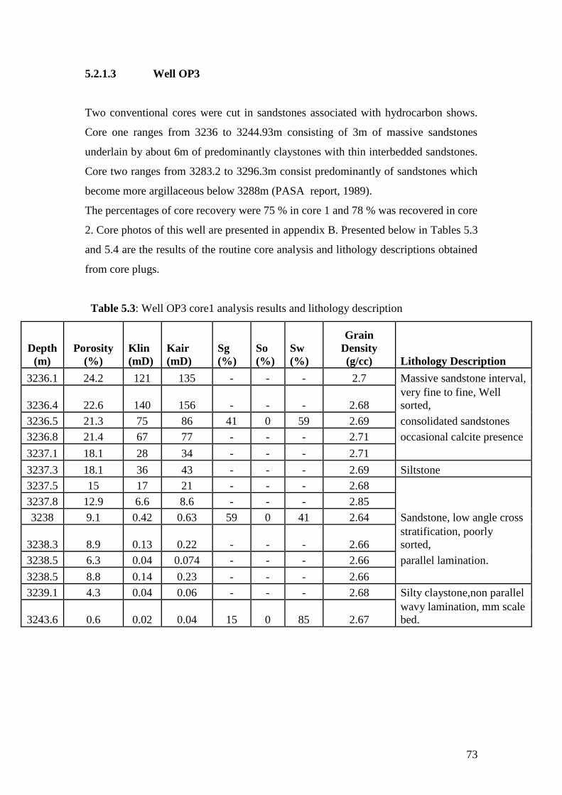
73

5.2.1.3 Well OP3

Two conventional cores were cut in sandstones associated with hydrocarbon shows.

Core one ranges from 3236 to 3244.93m consisting of 3m of massive sandstones

underlain by about 6m of predominantly claystones with thin interbedded sandstones.

Core two ranges from 3283.2 to 3296.3m consist predominantly of sandstones which

become more argillaceous below 3288m (PASA report, 1989).

The percentages of core recovery were 75 % in core 1 and 78 % was recovered in core

2. Core photos of this well are presented in appendix B. Presented below in Tables 5.3

and 5.4 are the results of the routine core analysis and lithology descriptions obtained

from core plugs.

Table 5.3: Well OP3 core1 analysis results and lithology description

Depth

(m)

Porosity

(%)

Klin

(mD)

Kair

(mD)

Sg

(%)

So

(%)

Sw

(%)

Grain

Density

(g/cc) Lithology Description

3236.1 24.2 121 135 - - - 2.7 Massive sandstone interval,

3236.4 22.6 140 156 - - - 2.68

very fine to fine, Well

sorted,

3236.5 21.3 75 86 41 0 59 2.69 consolidated sandstones

3236.8 21.4 67 77 - - - 2.71 occasional calcite presence

3237.1 18.1 28 34 - - - 2.71

3237.3 18.1 36 43 - - - 2.69 Siltstone

3237.5 15 17 21 - - - 2.68

3237.8 12.9 6.6 8.6 - - - 2.85

3238 9.1 0.42 0.63 59 0 41 2.64 Sandstone, low angle cross

3238.3 8.9 0.13 0.22 - - - 2.66

stratification, poorly

sorted,

3238.5 6.3 0.04 0.074 - - - 2.66 parallel lamination.

3238.5 8.8 0.14 0.23 - - - 2.66

3239.1 4.3 0.04 0.06 - - - 2.68 Silty claystone,non parallel

3243.6 0.6 0.02 0.04 15 0 85 2.67

wavy lamination, mm scale

bed.

74

Table 5.4: Well OP3 core 2 Routine core analysis results and lithology description.

Depth

(m)

Porosity

(%)

Klin

(mD)

Kair

(mD)

Sg

(%)

So

(%)

Sw

(%)

Grain

Density

(g/cc)

Lithology

Description

3283.2 19.2 3.7 4.9 30 0 70 2.68 Silty sandstone, poorly

3283.6 17.8 12 15 - - - 2.68

sorted, pararell

lamination

3283.85 17.8 25 30 - - - 2.68

3284.1 20.4 35 41 - - - 2.68

Sandstone, poorly

sorted with rip up

3284.35 21.3 34 40 - 2.68 clasts, very fine to

3284.45 22 53 62 36 0 64 2.68 fine.

3285.05 22.2 43 50 2.69

3285.3 22.8 40 47 2.67

3285.34 20.6 12 15 41 0 59 2.67

3285.83 17.3 3.6 4.8 2.69

3286.08 14.3 38 45 2.67

3286.3 20.4 45 53 2.68

3286.55 22.3 41 48 2.69

3286.6 22.2 69 79 39 0 61 2.68

3287.25 23.3 1.9 2.7 2.69

3287.3 15.8 67 77 2.67 Clay mudstone,

3287.9 3.7 0.12 0.194 45 0 55 2.66 burrowed horizontally.

3290.06 2.3 0.01 0.013 16 84 2.69

Claystones and

siltstone,

3291.76 2.7 0.01 0.016 35 65 2.65

Vertical burrows,

siderite concretion.

3292.79 2.6 0.01 0.023 35 65 2.66

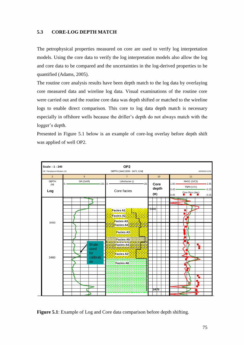
75

5.3 CORE-LOG DEPTH MATCH

The petrophysical properties measured on core are used to verify log interpretation

models. Using the core data to verify the log interpretation models also allow the log

and core data to be compared and the uncertainties in the log-derived properties to be

quantified (Adams, 2005).

The routine core analysis results have been depth match to the log data by overlaying

core measured data and wireline log data. Visual examinations of the routine core

were carried out and the routine core data was depth shifted or matched to the wireline

logs to enable direct comparison. This core to log data depth match is necessary

especially in offshore wells because the driller‟s depth do not always match with the

logger‟s depth.

Presented in Figure 5.1 below is an example of core-log overlay before depth shift

was applied of well OP2.

Figure 5.1: Example of Log and Core data comparison before depth shifting.

OP2Scale : 1 : 240


2

DEPTH

(M)

5

GR (GAPI)0. 150.

7

Lithofacies ()0. 28.

10 11

RHOZ (G/C3)1.95 2.95

TNPH (V/V)0.45 -0.15

Core Poro (dec)0.45 -0.15

3450

Facies A1

Facies A2

Facies A3

Facies A4

Facies A3

Facies A5

Facies A4

Facies A2

Facies A6

Core

depth

(M)Log

3446

3470

3460

Core facies

Shale

used

for

calibrati

on

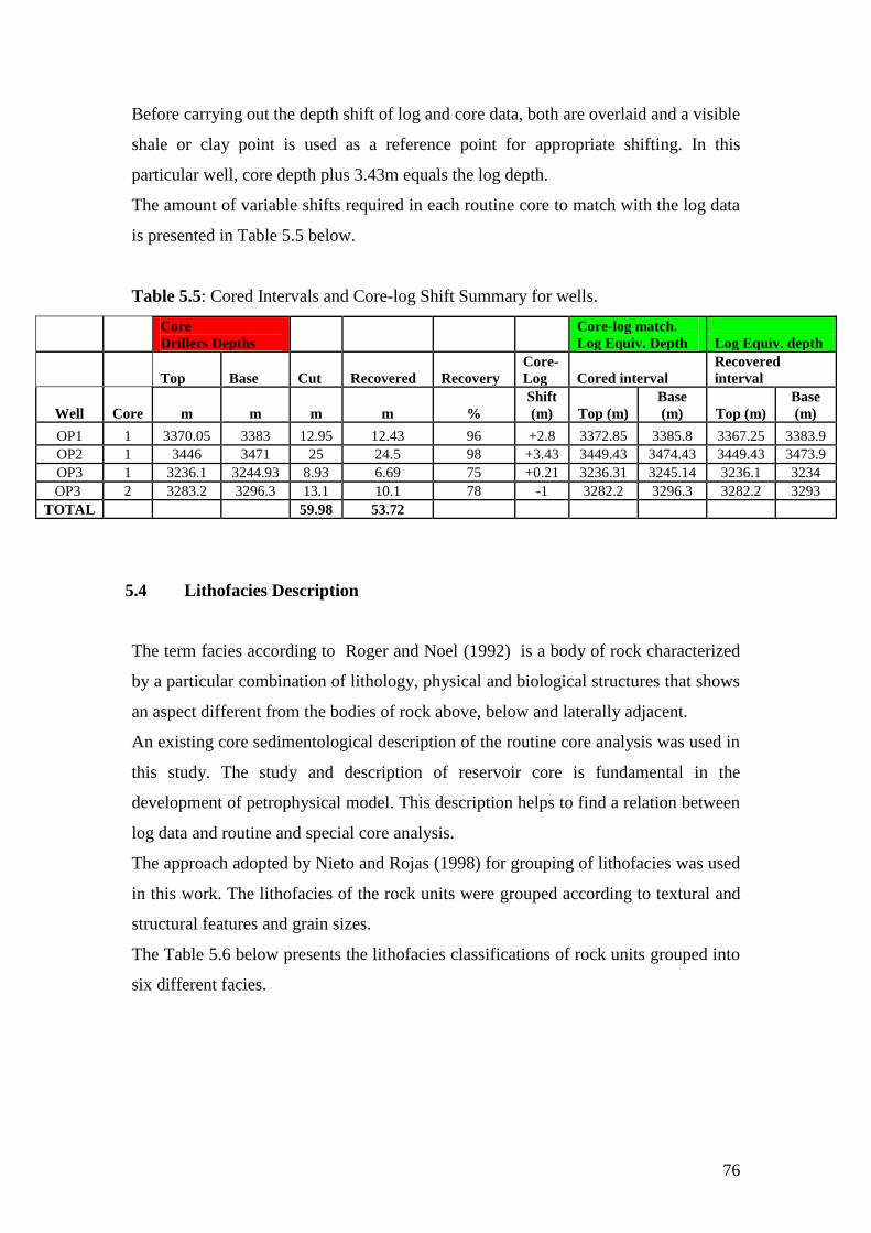
76

Before carrying out the depth shift of log and core data, both are overlaid and a visible

shale or clay point is used as a reference point for appropriate shifting. In this

particular well, core depth plus 3.43m equals the log depth.

The amount of variable shifts required in each routine core to match with the log data

is presented in Table 5.5 below.

Table 5.5: Cored Intervals and Core-log Shift Summary for wells.

Core

Drillers Depths Core-log match.

Log Equiv. Depth Log Equiv. depth

Top Base Cut Recovered Recovery

Core-

Log Cored interval

Recovered

interval

Well Core m m m m %

Shift

(m) Top (m)

Base

(m) Top (m)

Base

(m)

OP1 1 3370.05 3383 12.95 12.43 96 +2.8 3372.85 3385.8 3367.25 3383.9

OP2 1 3446 3471 25 24.5 98 +3.43 3449.43 3474.43 3449.43 3473.9

OP3 1 3236.1 3244.93 8.93 6.69 75 +0.21 3236.31 3245.14 3236.1 3234

OP3 2 3283.2 3296.3 13.1 10.1 78 -1 3282.2 3296.3 3282.2 3293

TOTAL 59.98 53.72

5.4 Lithofacies Description

The term facies according to Roger and Noel (1992) is a body of rock characterized

by a particular combination of lithology, physical and biological structures that shows

an aspect different from the bodies of rock above, below and laterally adjacent.

An existing core sedimentological description of the routine core analysis was used in

this study. The study and description of reservoir core is fundamental in the

development of petrophysical model. This description helps to find a relation between

log data and routine and special core analysis.

The approach adopted by Nieto and Rojas (1998) for grouping of lithofacies was used

in this work. The lithofacies of the rock units were grouped according to textural and

structural features and grain sizes.

The Table 5.6 below presents the lithofacies classifications of rock units grouped into

six different facies.

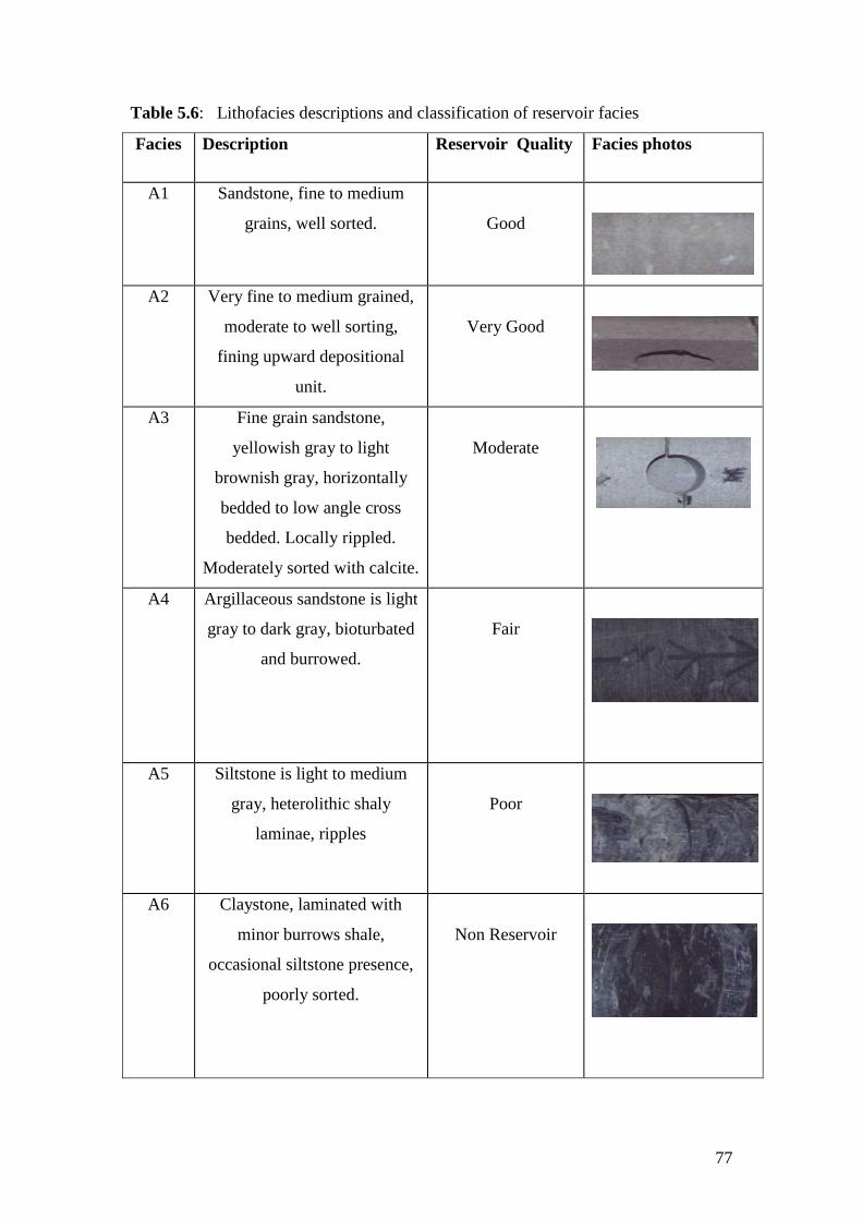
77

Table 5.6: Lithofacies descriptions and classification of reservoir facies

Facies Description Reservoir Quality Facies photos

A1 Sandstone, fine to medium

grains, well sorted.

Good

A2 Very fine to medium grained,

moderate to well sorting,

fining upward depositional

unit.

Very Good

A3 Fine grain sandstone,

yellowish gray to light

brownish gray, horizontally

bedded to low angle cross

bedded. Locally rippled.

Moderately sorted with calcite.

Moderate

A4 Argillaceous sandstone is light

gray to dark gray, bioturbated

and burrowed.

Fair

A5 Siltstone is light to medium

gray, heterolithic shaly

laminae, ripples

Poor

A6 Claystone, laminated with

minor burrows shale,

occasional siltstone presence,

poorly sorted.

Non Reservoir

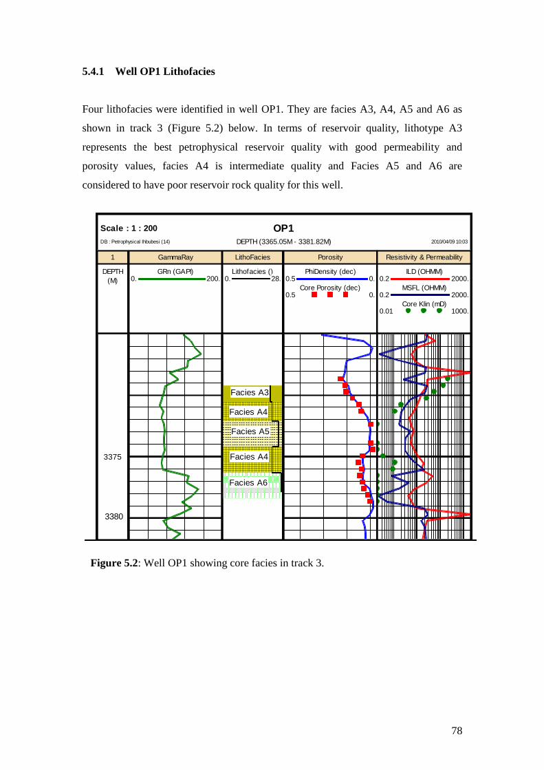
78

5.4.1 Well OP1 Lithofacies

Four lithofacies were identified in well OP1. They are facies A3, A4, A5 and A6 as

shown in track 3 (Figure 5.2) below. In terms of reservoir quality, lithotype A3

represents the best petrophysical reservoir quality with good permeability and

porosity values, facies A4 is intermediate quality and Facies A5 and A6 are

considered to have poor reservoir rock quality for this well.

OP1Scale : 1 : 200


1

DEPTH

(M)

GammaRay

GRn (GAPI)0. 200.

LithoFacies


Porosity

PhiDensity (dec)0.5 0.

Core Porosity (dec)0.5 0.

Resistivity & Permeability

ILD (OHMM)0.2 2000.


Core Klin (mD)0.01 1000.

3375

Facies A3

Facies A4

Facies A5

Facies A4

Facies A6

3380

Figure 5.2: Well OP1 showing core facies in track 3.

79


In well OP2, six lithofacies were identified, they are A1, A2, A3, A4, A5, and A6 as

shown in track 6 (Figure 5.3) below. The best reservoir rock quality are facies A1 and

A2, while A3 and A4 can be considered good quality, A5 is classified as poor

reservoir rock quality and A6 is not considered as a reservoir rock.

Figure 5.3: Well OP2 graphics showing core facies in track 3.

OP2Scale : 1 : 250


Depth

DEPTH

(M)

GammaRay

GRn (GAPI)0. 200.

Core Facies


Porosity

PhiDen (dec)0.5 0.

Core Poro (dec)0.5 0.


AT10 (OHMM)0.2 2000.

AT90 (OHMM)0.2 2000.

Cor Kli (mD)0.001 10000.

3450 Facies A1

Facies A2

Facies A3

Facies A4

Facies A3

Facies A5

Facies A4

Facies A2

Facies A6

3460

3470

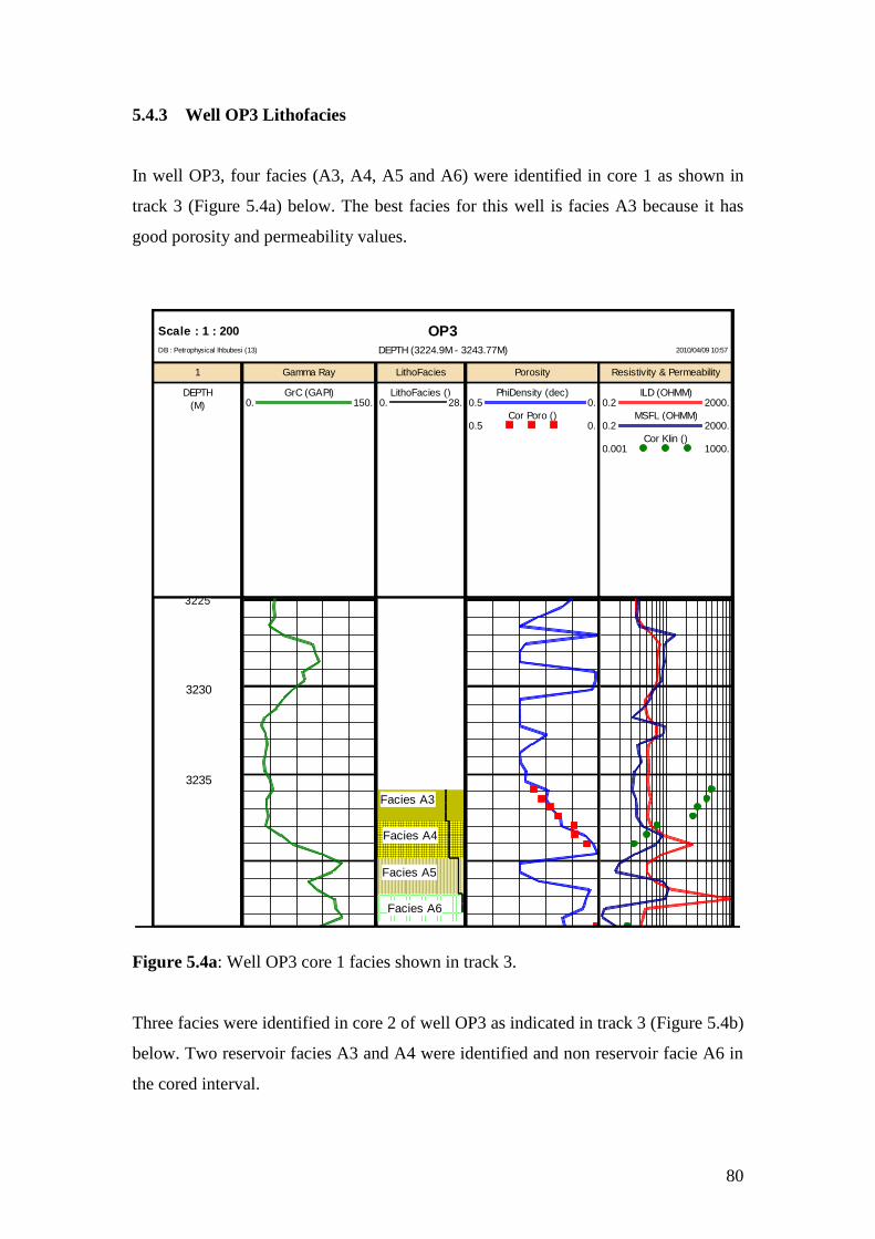
80


In well OP3, four facies (A3, A4, A5 and A6) were identified in core 1 as shown in

track 3 (Figure 5.4a) below. The best facies for this well is facies A3 because it has

good porosity and permeability values.

OP3Scale : 1 : 200


1

DEPTH

(M)

Gamma Ray

GrC (GAPI)0. 150.

LithoFacies

LithoFacies ()0. 28.

Porosity


Cor Poro ()0.5 0.


ILD (OHMM)0.2 2000.


Cor Klin ()0.001 1000.

3225

Facies A3

Facies A4

Facies A5

Facies A6

3230

3235

Figure 5.4a: Well OP3 core 1 facies shown in track 3.

Three facies were identified in core 2 of well OP3 as indicated in track 3 (Figure 5.4b)

below. Two reservoir facies A3 and A4 were identified and non reservoir facie A6 in

the cored interval.

81

OP3Scale : 1 : 200


1

DEPTH

(M)

Gamma Ray

GrC (GAPI)0. 150.

LithoFacies

Core Facies ()0. 28.


Porosity


Cor Poro ()0.5 0.


ILD (OHMM)0.2 2000.


Cor Klin ()0.001 1000.

3275

Facies A3

Facies A4

Facies A5

Facies A6

Facies A4

Facies A3

Facies A6

3285

Figure 5.4b: Well OP3 core 2 facies shown in track 3.

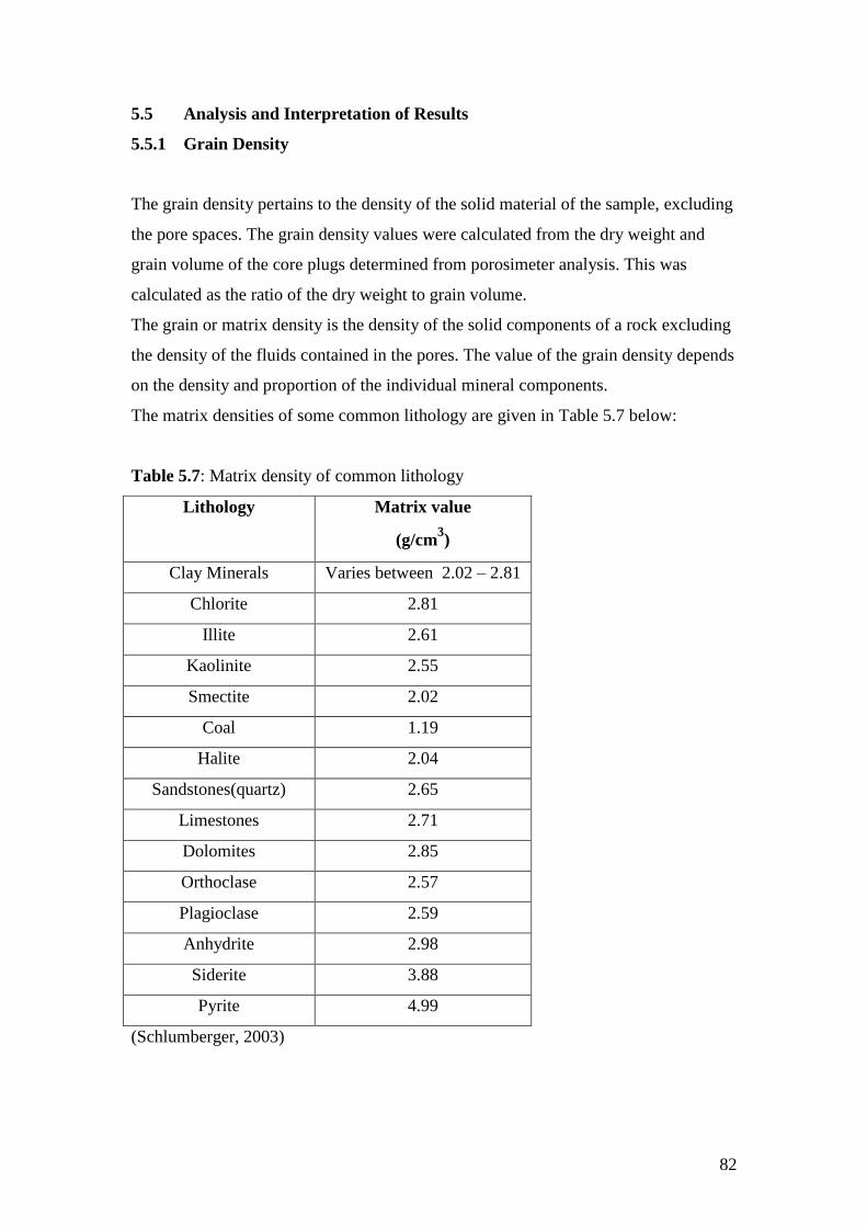
82

5.5 Analysis and Interpretation of Results

5.5.1 Grain Density

The grain density pertains to the density of the solid material of the sample, excluding

the pore spaces. The grain density values were calculated from the dry weight and

grain volume of the core plugs determined from porosimeter analysis. This was

calculated as the ratio of the dry weight to grain volume.

The grain or matrix density is the density of the solid components of a rock excluding

the density of the fluids contained in the pores. The value of the grain density depends

on the density and proportion of the individual mineral components.

The matrix densities of some common lithology are given in Table 5.7 below:

Table 5.7: Matrix density of common lithology

Lithology Matrix value

(g/cm3)

Clay Minerals Varies between 2.02 – 2.81

Chlorite 2.81

Illite 2.61

Kaolinite 2.55

Smectite 2.02

Coal 1.19

Halite 2.04

Sandstones(quartz) 2.65

Limestones 2.71

Dolomites 2.85

Orthoclase 2.57

Plagioclase 2.59

Anhydrite 2.98

Siderite 3.88

Pyrite 4.99

(Schlumberger, 2003)

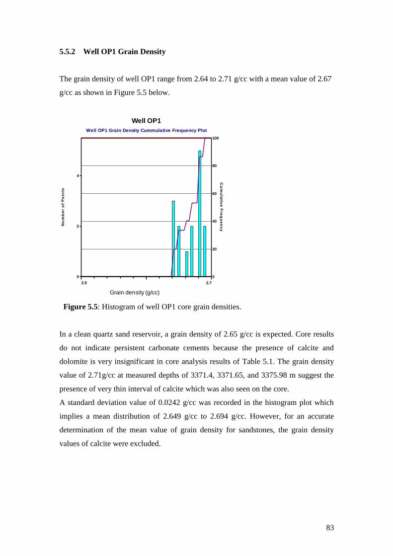
83

5.5.2 Well OP1 Grain Density

The grain density of well OP1 range from 2.64 to 2.71 g/cc with a mean value of 2.67

g/cc as shown in Figure 5.5 below.

Well OP1

Well OP1 Grain Density Cummulative Frequency Plot

0

20

40

60

80

100

Cu

mu

lativ

e F

req

ue

nc

y

2.5 2.7

0

2

4

Nu

mb

er

of

Po

ints

Grain density (g/cc)

Figure 5.5: Histogram of well OP1 core grain densities.

In a clean quartz sand reservoir, a grain density of 2.65 g/cc is expected. Core results

do not indicate persistent carbonate cements because the presence of calcite and

dolomite is very insignificant in core analysis results of Table 5.1. The grain density

value of 2.71g/cc at measured depths of 3371.4, 3371.65, and 3375.98 m suggest the

presence of very thin interval of calcite which was also seen on the core.

A standard deviation value of 0.0242 g/cc was recorded in the histogram plot which

implies a mean distribution of 2.649 g/cc to 2.694 g/cc. However, for an accurate

determination of the mean value of grain density for sandstones, the grain density

values of calcite were excluded.

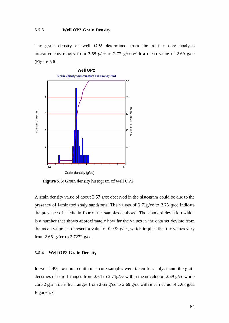
84


The grain density of well OP2 determined from the routine core analysis

measurements ranges from 2.58 g/cc to 2.77 g/cc with a mean value of 2.69 g/cc

(Figure 5.6).

Well OP2

Grain Density Cummulative Frequency Plot

0

20

40

60

80

100

Cu

mu

lativ

e F

req

ue

nc

y

2.5 3.

0

2

4

6

8

Nu

mb

er

of

Po

ints

Grain density (g/cc)

Figure 5.6: Grain density histogram of well OP2

A grain density value of about 2.57 g/cc observed in the histogram could be due to the

presence of laminated shaly sandstone. The values of 2.71g/cc to 2.75 g/cc indicate

the presence of calcite in four of the samples analysed. The standard deviation which

is a number that shows approximately how far the values in the data set deviate from

the mean value also present a value of 0.033 g/cc, which implies that the values vary

from 2.661 g/cc to 2.7272 g/cc.


In well OP3, two non-continuous core samples were taken for analysis and the grain

densities of core 1 ranges from 2.64 to 2.71g/cc with a mean value of 2.69 g/cc while

core 2 grain densities ranges from 2.65 g/cc to 2.69 g/cc with mean value of 2.68 g/cc

Figure 5.7.

85

Well OP3

Core 1 Grain Density Cummulative Frequency Plot

0

20

40

60

80

100

Cu

mu

lativ

e F

req

ue

nc

y

2.5 3.

0

2

Nu

mb

er

of

Po

ints

Well OP3

Core 2 Grain Density Cummulative Frequency Plot

0

20

40

60

80

100C

um

ula

tive

Fre

qu

en

cy

2.5 3.

0

2

4

6

Nu

mb

er

of

Po

ints

Grain density (g/cc)Grain density (g/cc)

Figure 5.7: Well OP3 core grain density cumulative frequency plot.

The grain density values recorded in core 1 display higher standard deviation value of

0.05 g/cc from the mean which gives a range of 2.64 g/cc to 2.74 g/cc. The high

standard deviation value recorded in core 1 may be due to the presence of calcite in

two of the samples analysed. The low standard deviation value of about 0.01198 g/cc

recorded in core 2 implies a mean range of 2.68 g/cc to 2.71g/cc.

5.5.5 Comparison of Grain Density Distributions for Wells

The grain density value for all the wells with core analysis results showed a range of

2.58 g/cc to 2.76 g/cc with mean value of 2.68 g/cc and standard deviation value of

0.028 g/cc (Figure 5.8) which means variation 2.65 g/cc to 2.71g/cc . The presence of

calcite was observed in all the cored wells with relatively small proportion .Well OP2

showed the highest mean grain density with mean value of 2.69 g/cc as against values

of about 2.67 g/cc recorded in well OP1 and OP3 respectively. The mean grain

density of 2.67 g/cc was obtained from the analysis, excluding that of calcite which

will be adopted as the matrix grain density for log analysis.

86

5.6 Interpretation of Core Porosity

The porosity of a reservoir rock was defined in chapter three as the percentage of the

volume of the rock that is not occupied by the solid framework of the reservoir. This

determines the amount of water or other fluids that a rock can contain. Fraser and

Graton (1935) determined the porosity of various packing arrangements of uniform

spheres and concluded that the cubic packed system has a porosity of 47.6 % and the

rhombohedra or closed packed system has a porosity of 25.9 %.

After cleaning of the core plugs and removal of fluids, porosity is determined from the

grain volume and the bulk volume of the sample. Depending on the technique used,

different types of porosity are estimated. With a gas expansion method, the connected

porosity is measured, while the destruction of the sample to estimate grain volume, a

measure of total porosity is obtained.

Determination of the core plug porosities for the wells was done using helium gas

based on Boyle‟s law for gas expansion (P1 V1 =P2 V2). Porosity measurement by gas

expansion indicates only pores that are interconnected (effective porosity) thereby

All Well Grain Density Histogram Plot

-

0

20

40

60

80

100

Cumulative F requency

2.5 3. 0

10

20

Number of Points

Well Mean Std Dev

OP1 2.6717 0.02243

OP2 2.6946 0.03345

OP3 2.6761 0.01627

All Zones 2.6832 0.02812

2.68 g/cc

Figure 5.8: Grain density histogram plot for well OP1, OP2 and OP3

Grain Density (g/cc)

87

providing a very good estimate of effective porosity for the purpose of reservoir

evaluation.

The porosities of petroleum reservoirs range from about 5 % to 45 % and factors

determining the magnitude of porosity in sediments are grain sorting, degree of

cementation or consolidation, amount of compaction and methods of grain packing

(Djebbar, 1999). If all the grains are of the same size, sorting is said to be good and

porosity may be high. If grains are of many sizes and are mixed together, sorting is

regarded as poor and porosity in that condition will be reduced. Poorly sorted

sediments usually have lower porosity because the fine grained fragments tend to fill

in the open space.

Cementation that takes place during diagenesis also tends to fill in the pore space, so

highly cemented sedimentary rocks have lower porosity than poorly cemented

sedimentary rocks. Although, round grains and a high content of grain cement gives a

high porosity, and angular grains and low cement content gives lower porosity.

5.6.1 Well OP1 Porosity

The core porosity values of well OP1 ranges from 1.2 % to 20.2 % at the cored

interval. The low porosity values were observed in intervals that are associated with

claystones and siltstone interbedded lamina. The relatively high porosity interval was

observed in massive sandstones intervals that are very fine to fine grains and are well

sorted as observed in depth of 3368.5 to 3369.2 m (Figure 5.9a). In this well, the

decrease in porosity is observed in the rocks associated with clay. The core porosity

histogram of well OP1 is given in Figure 5.9b below.

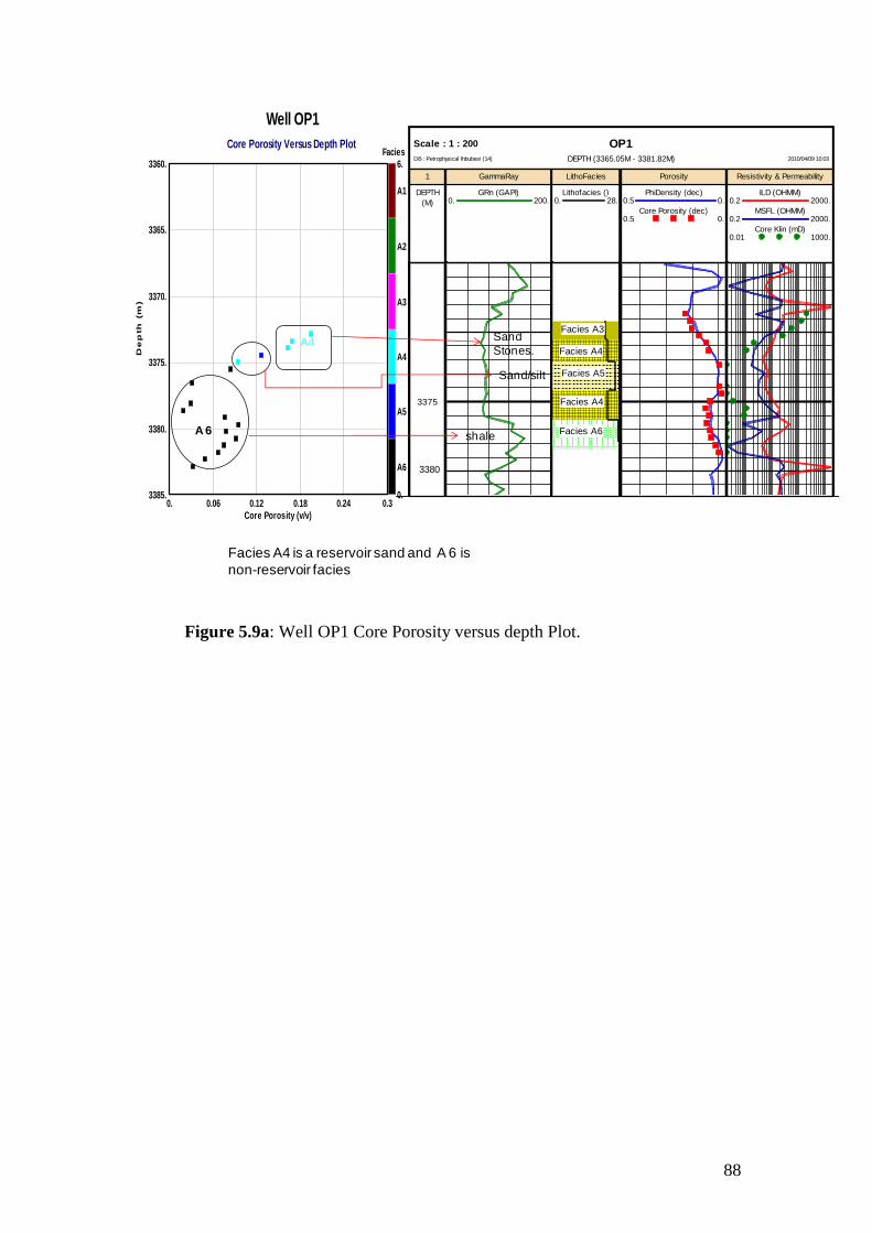
88

OP1Scale : 1 : 200


1

DEPTH

(M)

GammaRay

GRn (GAPI)0. 200.

LithoFacies


Porosity




ILD (OHMM)0.2 2000.



3375

Facies A3

Facies A4

Facies A5

Facies A4

Facies A6

3380

Well OP1

Core Porosity Versus Depth Plot

0. 0.06 0.12 0.18 0.24 0.3

Core Porosity (v/v)

3385.

3380.

3375.

3370.

3365.

3360.

De

pth

(m

)

A6

A5

A4

A3

A2

A1

0.

6.

Facies

Sand

Stones.

Sand/silt

shaleA 6

A4

Facies A4 is a reservoir sand and A 6 is

non-reservoir facies

Figure 5.9a: Well OP1 Core Porosity versus depth Plot.

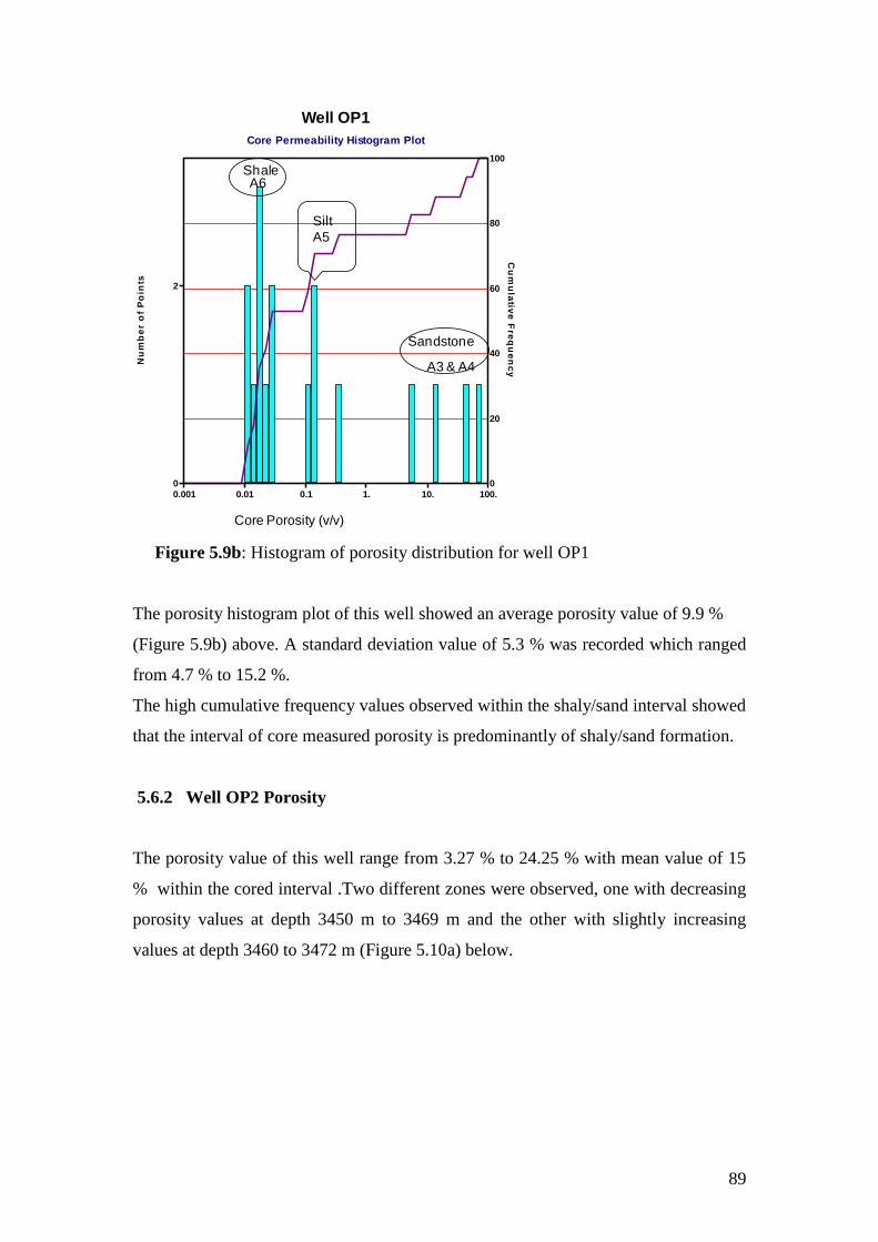
89

Well OP1

Core Permeability Histogram Plot

0

20

40

60

80

100

Cu

mu

lativ

e F

req

ue

nc

y

0.001 0.01 0.1 1. 10. 100.

0

2

Nu

mb

er

of

Po

ints

Sandstone

Shale

A3 & A4

Silt

A5

A6

Core Porosity (v/v)

Figure 5.9b: Histogram of porosity distribution for well OP1

The porosity histogram plot of this well showed an average porosity value of 9.9 %

(Figure 5.9b) above. A standard deviation value of 5.3 % was recorded which ranged

from 4.7 % to 15.2 %.

The high cumulative frequency values observed within the shaly/sand interval showed

that the interval of core measured porosity is predominantly of shaly/sand formation.


The porosity value of this well range from 3.27 % to 24.25 % with mean value of 15

% within the cored interval .Two different zones were observed, one with decreasing

porosity values at depth 3450 m to 3469 m and the other with slightly increasing

values at depth 3460 to 3472 m (Figure 5.10a) below.

90

Figure 5.10a: Well OP2 porosity versus depth plot.

The high porosity intervals are medium fine and well sorted sandstones, while the low

porosity values are associated with laminated shaly intervals.

On the porosity histogram, a bimodal frequency were observed showing the shaly/silt

mode and the clean sandstone mode, with mean value of about 15 % recorded within

the cored interval with standard deviation value of about 8.4% which implies a

variation of 6.8 % to 23.7 % (Figure 5.10b).

Well OP2

Core Porosity Versus Depth and Facies Plot

0. 0.06 0.12 0.18 0.24 0.3

Core Porosity (v/v)

3476.

3469.

3462.

3455.

3448.

3441.

De

pth

(m

)

A6

A5

A4

A3

A2

A1

0.

6.Facies

A6

A6 & A5

A1 & A2

A3 &A4

A2

OP2Scale : 1 : 250


Depth

DEPTH

(M)

GammaRay

GRn (GAPI)0. 200.

Core Facies


Porosity

PhiDen (dec)0.5 0.



AT10 (OHMM)0.2 2000.

AT90 (OHMM)0.2 2000.

Cor Kli (mD)0.001 10000.

3450 Facies A1

Facies A2

Facies A3

Facies A4

Facies A3

Facies A5

Facies A4

Facies A2

Facies A6

3460

3470

Massive

sands

Shale/Silt

Sandstone

Shale

91

Well OP2

Core Porosity Histogram

0

20

40

60

80

100

Cu

mu

lativ

e F

req

ue

nc

y

0.001 0.3

0

2

4

Nu

mb

er

of

Po

ints

Clean

Sands

Shale/Silt

0.240.180.120.06

A1,A2 &

A3

A5 & A6

Core Porosity (v/v)

Figure 5.10b: Well OP2 core porosity histogram and plot against depth.

The differences in variations of porosity in the zones may be attributed to the type of

facies present in each zone. The interval of porosity values less than 6 % is comprised

mostly of facies A5 and A6 which is shaly/silt and shale intervals. The interval with

porosity values of more than 18 % is comprised of the clean sandstones of facies A1,

A2 and A3 respectively.


The porosity value of well OP3 ranged from 0.6 % to 24.2 % in core 1 and 2.3 % to

23.3 % in core 2 within the cored intervals. The silty claystones interval in core 1

contribute to the low porosity values observed while the massive sandstone units that

are very fine to fine, well sorted with occasional calcite intervals are with high

porosity values (Figure 5.11a).

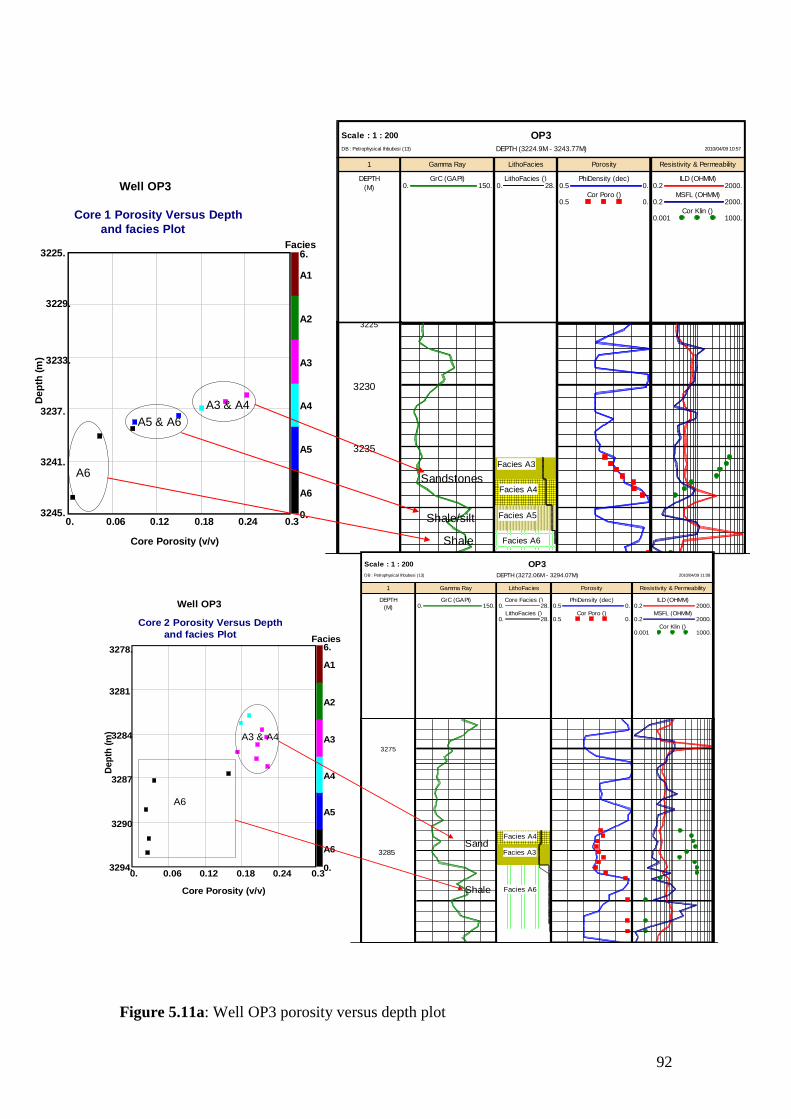
92

Figure 5.11a: Well OP3 porosity versus depth plot

OP3Scale : 1 : 200


1

DEPTH

(M)

Gamma Ray

GrC (GAPI)0. 150.

LithoFacies


Porosity


Cor Poro ()0.5 0.


ILD (OHMM)0.2 2000.


Cor Klin ()0.001 1000.

3225

Facies A3

Facies A4

Facies A5

Facies A6

3230

3235

Well OP3

Core 1 Porosity Versus Depth

and facies Plot

0. 0.06 0.12 0.18 0.24 0.3

Core Porosity (v/v)

3245.

3241.

3237.

3233.

3229.

3225.

De

pth

(m

)

A6

A5

A4

A3

A2

A1

0.

6.Facies

A3 & A4

A5 & A6

A6Sandstones

Shale/silt

Shale

OP3Scale : 1 : 200


1

DEPTH

(M)

Gamma Ray

GrC (GAPI)0. 150.

LithoFacies



Porosity


Cor Poro ()0.5 0.


ILD (OHMM)0.2 2000.


Cor Klin ()0.001 1000.

3275

Facies A3

Facies A4

Facies A5

Facies A6

Facies A4

Facies A3

Facies A6

3285

Well OP3

Core 2 Porosity Versus Depth

and facies Plot

0. 0.06 0.12 0.18 0.24 0.3

Core Porosity (v/v)

3294.

3290

3287

3284

3281

3278.

Dep

th (

m)

A6

A5

A4

A3

A2

A1

0.

6.Facies

A6

A3 & A4

Sand

Shale

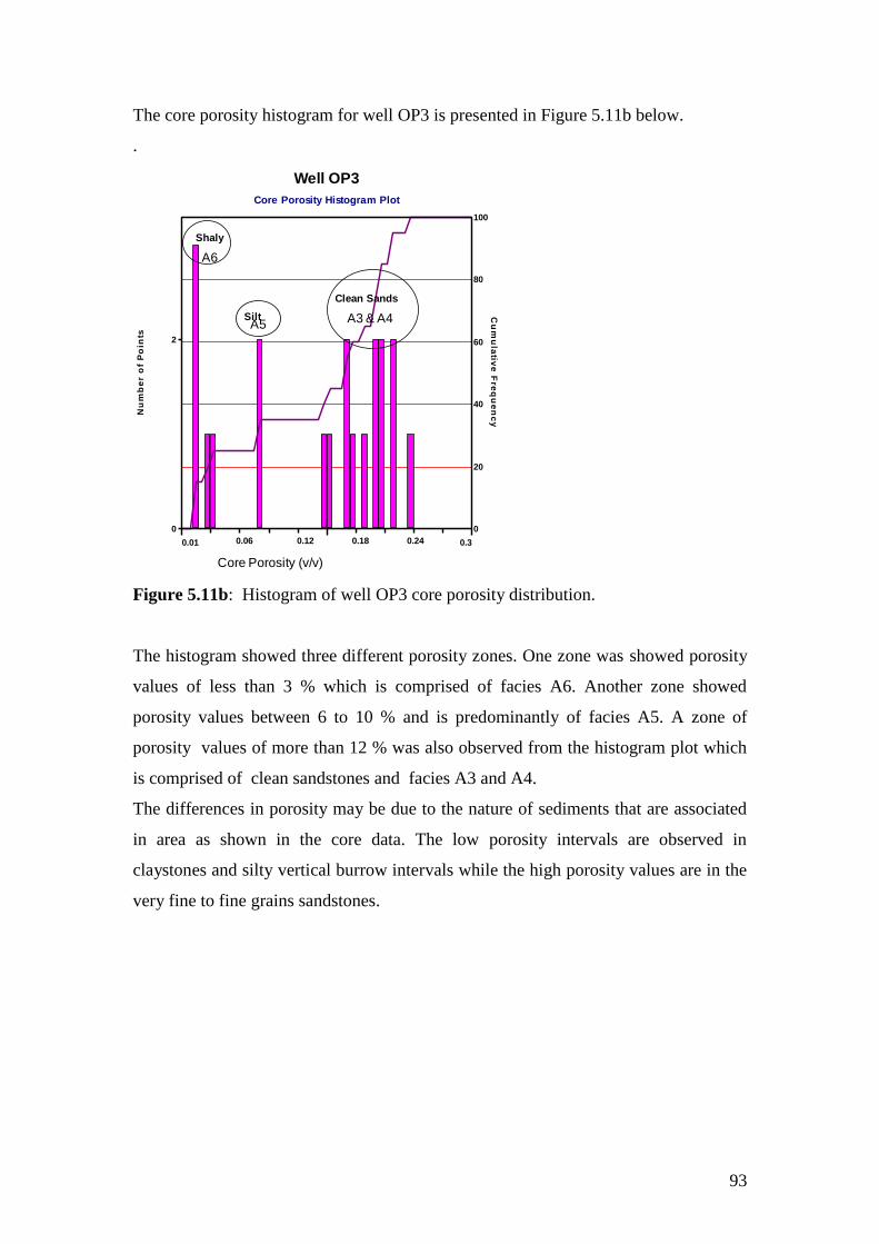
93

The core porosity histogram for well OP3 is presented in Figure 5.11b below.

.

Well OP3

Core Porosity Histogram Plot

0

20

40

60

80

100

Cu

mu

lativ

e F

req

ue

nc

y

0.01 0.3

0

2

Nu

mb

er

of

Po

ints

Clean Sands

Silt

Shaly

0.240.180.120.06

A3 & A4

A6

A5

Core Porosity (v/v)

Figure 5.11b: Histogram of well OP3 core porosity distribution.

The histogram showed three different porosity zones. One zone was showed porosity

values of less than 3 % which is comprised of facies A6. Another zone showed

porosity values between 6 to 10 % and is predominantly of facies A5. A zone of

porosity values of more than 12 % was also observed from the histogram plot which

is comprised of clean sandstones and facies A3 and A4.

The differences in porosity may be due to the nature of sediments that are associated

in area as shown in the core data. The low porosity intervals are observed in

claystones and silty vertical burrow intervals while the high porosity values are in the

very fine to fine grains sandstones.

94

5.6.4 Porosity distribution for wells

The histogram of porosity distribution for all wells is presented in Figure 5.12a below.

All Well

Core Porosity Histogram PlotMulti-well Interval histogram

0

20

40

60

80

100

Cu

mu

lativ

e F

req

uen

cy

0.01 0.30

2

4

Nu

mb

er

of P

oin

ts

Well Mean Std Dev

OP1 0.08753 0.05128

OP2 0.155 0.08565

OP3 0.14435 0.07752

All Zones 0.135 0.08

0.240.180.120.06

A6

A5

A4 &

A3

A2 &

A1

Core Porosity (v/v)

Figure 5.12a: Histogram of Porosity distribution for wells.

Two distinct areas were observed on the histogram, an area of low porosity values

and an area of high porosity values. The zone of porosity values of less than 10 % is

comprised of facies A6 and A5. The area of porosity values between 12 to 18 % is

comprised of facies A4 and A3, while facies A2 and A1 dominates the intervals

with porosity values greater than 18 %.

An average porosity value of 13.5 % was recorded on the histogram plot with a

corresponding standard deviation value of 7%.

The low porosity values recorded are due to the presence of clay/silt in such

intervals while the high porosity values are associated with clean sandstone

intervals.

The histogram plot of the low porosity interval is presented in Figure 5.12b below.

95

All Well

Core Porosity (Shale and Siltstone Interval) Histogram PlotMulti-well Interval histogram

0

20

40

60

80

100

Cu

mu

lativ

e F

req

uen

cy

0.01 0.140

2

Nu

mb

er

of P

oin

ts

Well Mean Std Dev

OP1 0.0685 0.03132

OP2 0.05162 0.02142

OP3 0.04786 0.02928

All Zones 0.05798 0.02834

0.075

Shaly/Silt

Shaly A6

A5

Core Porosity (v/v)

Figure 5.12b: Histogram of Core Porosity Shaly/Silt interval for all well.

The low porosity values were dominant in well OP1 within the shale and siltstone

intervals of the histogram and generally features in entire well. The plot clearly

showed the distinctions between the shaly and silty intervals with an intermediary

porosity value of approximately 6 % .

The high porosity value as plotted in the histogram (Figure 5.12c) below shows area

of massive sandstone intervals with well sorted grains that are well sorted with

medium to fine grains in the well.

96

All Well

Core Porosity (Massive Sands Interval) Histogram PlotMulti-well Interval histogram

0

20

40

60

80

100

Cu

mu

lativ

e F

req

uen

cy

0.14 0.30

2

4

Nu

mb

er

of P

oin

tsWell Mean Std Dev

OP1 0.17633 0.01721

OP20.22029 0.01795

OP30.19631 0.02702

All Zones 0.20762 0.0259

0.22

Facies A1 ,A2 ,A3 and A4

Core Porosity (v/v)

Figure 5.12c: Histogram of core porosity massive sands for Wells.

The histogram plot present well OP2 as the dominant well in the most porous

intervals of the plot and well OP3 with the least porosity values recorded in the

interval.

5.7 Interpretation of Permeability

The permeability of a rock which is the ability of the rock to allow fluids to flow

through its connected pores is controlled by rock grain size, grain shape, degree of

cementation or consolidation, grain packing, and clay. Permeability of reservoir rocks

may vary from less than 1 mD to over 1000 mD.

To determine the permeability of the core plugs, the plugs were placed in a compliant

sleeve within a cylinder. A pressure on the sleeve ensures that the injected gas or

liquid flows parallel to the core plug axis. Fluid, usually gas is injected with an inflow

pressure and flows almost linearly through the plug to atmospheric pressure. The

permeability is then determined from Darcy‟s law. Due to difference in flow physics

between gas and liquid especially in low permeable media, a correction is done on the

gas or air permeability which is known as Klinkenberg Correction. The permeability

values are reported as permeabilities to air and liquid (corrected for the Klinkenberg

97

effect). Gas permeability corrected for the Klinkenberg effect is considered equivalent

to the permeability if a liquid medium is present in the pores.

The quality of a reservoir as determined by permeability in mD may be scaled as

shown in the Table 5.8 below:

Table 5.8: Permeability classification scale

Permeability Values

(mD)

Classification

Less than 1 Poor

Between 1 and 10 Fair

Between 10 and 50 Moderate

Between 50 and 250 Good

Above 250 Very Good

(Modified after Djebbar, 1999)

5.7.1 Well OP1 Permeability

The permeability of well OP1 was measured horizontally and vertically. The

horizontally measured permeability is accepted as the rock permeability because it is

measured parallel to the bedding which is the major contributor to fluid flow into a

typical reservoir.

The permeability values of this well were reported as permeability to air and liquid

(corrected for the Klinkenberg effect). Gas permeability corrected for the Klinkenberg

effect is considered equivalent to the permeability if a liquid medium is otherwise

present in the pores. The air permeability values ranges from 0.01 mD to 108 mD and

the liquid permeability values from 0.01 mD to 96 mD. Air permeabilities measure

higher than the liquid permeabilities.

For consistencies, the liquid permeability values are used in this study. Plot of

permeability in log scale against depth in linear scale is given in Figure 5.13a below.

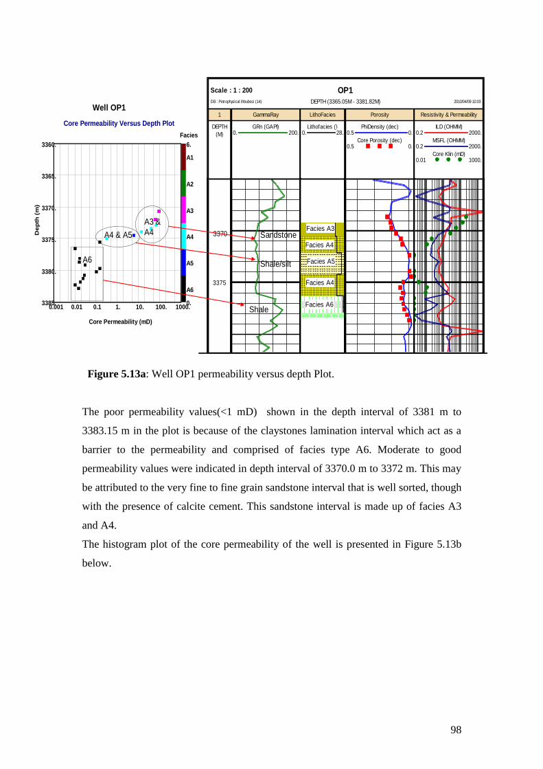
98

Figure 5.13a: Well OP1 permeability versus depth Plot.

The poor permeability values(<1 mD) shown in the depth interval of 3381 m to

3383.15 m in the plot is because of the claystones lamination interval which act as a

barrier to the permeability and comprised of facies type A6. Moderate to good

permeability values were indicated in depth interval of 3370.0 m to 3372 m. This may

be attributed to the very fine to fine grain sandstone interval that is well sorted, though

with the presence of calcite cement. This sandstone interval is made up of facies A3

and A4.

The histogram plot of the core permeability of the well is presented in Figure 5.13b

below.

OP1Scale : 1 : 200


1

DEPTH

(M)

GammaRay

GRn (GAPI)0. 200.

LithoFacies


Porosity




ILD (OHMM)0.2 2000.



3375

Facies A3

Facies A4

Facies A5

Facies A4

Facies A6

Well OP1

Core Permeability Versus Depth Plot

0.001 0.01 0.1 1. 10. 100. 1000.

Core Permeability (mD)

3385.

3380.

3375.

3370.

3365.

3360.

De

pth

(m

)

A6

A5

A4

A3

A2

A1

0.

6.

Facies

Sandstone

Shale/silt

Shale

3370

A3 &

A4A4 & A5

A6

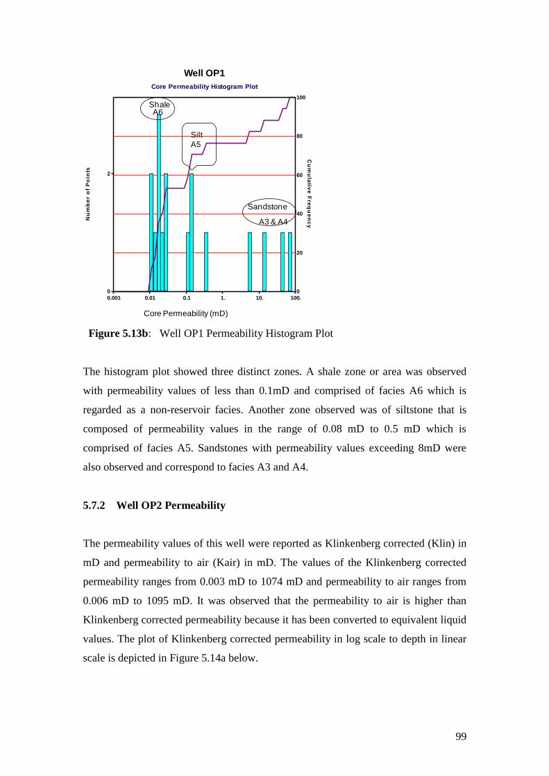
99

Well OP1


0

20

40

60

80

100

Cu

mu

lativ

e F

req

ue

nc

y

0.001 0.01 0.1 1. 10. 100.

0

2

Nu

mb

er

of

Po

ints

Sandstone

Shale

A3 & A4

Silt

A5

A6


Figure 5.13b: Well OP1 Permeability Histogram Plot

The histogram plot showed three distinct zones. A shale zone or area was observed

with permeability values of less than 0.1mD and comprised of facies A6 which is

regarded as a non-reservoir facies. Another zone observed was of siltstone that is

composed of permeability values in the range of 0.08 mD to 0.5 mD which is

comprised of facies A5. Sandstones with permeability values exceeding 8mD were

also observed and correspond to facies A3 and A4.


The permeability values of this well were reported as Klinkenberg corrected (Klin) in

mD and permeability to air (Kair) in mD. The values of the Klinkenberg corrected

permeability ranges from 0.003 mD to 1074 mD and permeability to air ranges from

0.006 mD to 1095 mD. It was observed that the permeability to air is higher than

Klinkenberg corrected permeability because it has been converted to equivalent liquid

values. The plot of Klinkenberg corrected permeability in log scale to depth in linear

scale is depicted in Figure 5.14a below.

100

Figure 5.14a: Well OP2 Depth versus permeability plot.

The massive clean sandstone interval present good to very good permeability values

and is associated with core facies types A1 and A2. The sand with sparingly

distributed siltstone interval showed fair to good permeability values which are

attributed to the presence of silt in the interval and corresponds to facies A3 and A4.

The silt interval lies between the sand and shaly interval and corresponds to facies A5.

A poor permeability interval was also observed in the plot and corresponds to the non-

reservoir facies A6. The permeability histogram (Figure 5.14b) is presented below.

Well OP2

Core Permeability Vs Depth and Facies

0.001 0.01 0.1 1. 10. 100. 1000. 10000.


3476.

3469.

3462.

3455.

3448.

3441.

De

pth

(m

)

A6

A5

A4

A3

A2

A1

0.

6.Facies

A6

A5 & A6

A1,A2,

A3 &

A4

OP2Scale : 1 : 250


Depth

DEPTH

(M)

GammaRay

GRn (GAPI)0. 200.

Core Facies


Porosity

PhiDen (dec)0.5 0.



AT10 (OHMM)0.2 2000.

AT90 (OHMM)0.2 2000.

Cor Kli (mD)0.001 10000.

3450 Facies A1

Facies A2

Facies A3

Facies A4

Facies A3

Facies A5

Facies A4

Facies A2

Facies A6

3460

3470

Massive

sands

Shale/silt

Sands

Shale

A2

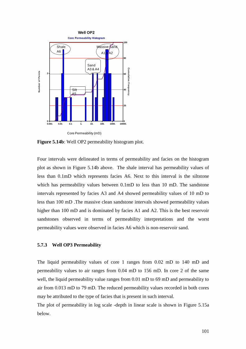
101

Well OP2

Core Permeability Histogram

0

20

40

60

80

100

Cu

mu

lativ

e F

req

ue

nc

y

0.001 0.01 0.1 1. 10. 100. 1000. 10000.

0

2

Nu

mb

er

of

Po

ints

Massive SandShale

A1 & A2A6

Sand

A3 & A4

Silt

A5


Figure 5.14b: Well OP2 permeability histogram plot.

Four intervals were delineated in terms of permeability and facies on the histogram

plot as shown in Figure 5.14b above. The shale interval has permeability values of

less than 0.1mD which represents facies A6. Next to this interval is the siltstone

which has permeability values between 0.1mD to less than 10 mD. The sandstone

intervals represented by facies A3 and A4 showed permeability values of 10 mD to

less than 100 mD .The massive clean sandstone intervals showed permeability values

higher than 100 mD and is dominated by facies A1 and A2. This is the best reservoir

sandstones observed in terms of permeability interpretations and the worst

permeability values were observed in facies A6 which is non-reservoir sand.


The liquid permeability values of core 1 ranges from 0.02 mD to 140 mD and

permeability values to air ranges from 0.04 mD to 156 mD. In core 2 of the same

well, the liquid permeability value ranges from 0.01 mD to 69 mD and permeability to

air from 0.013 mD to 79 mD. The reduced permeability values recorded in both cores

may be attributed to the type of facies that is present in such interval.

The plot of permeability in log scale -depth in linear scale is shown in Figure 5.15a

below.

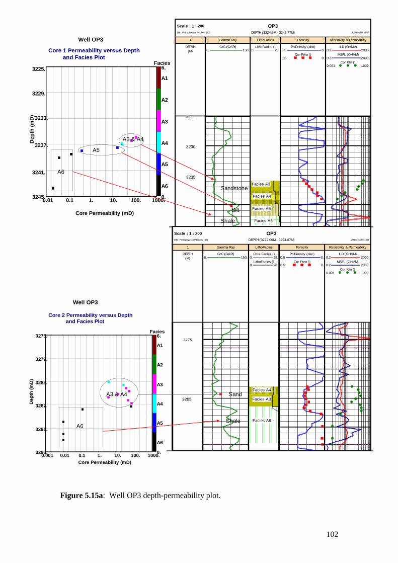
102

Figure 5.15a: Well OP3 depth-permeability plot.

OP3Scale : 1 : 200


1

DEPTH

(M)

Gamma Ray

GrC (GAPI)0. 150.

LithoFacies


Porosity


Cor Poro ()0.5 0.


ILD (OHMM)0.2 2000.


Cor Klin ()0.001 1000.

3225

Facies A3

Facies A4

Facies A5

Facies A6

3230

3235

Well OP3

Core 1 Permeability versus Depth

and Facies Plot

0.01 0.1 1. 10. 100. 1000.


3245.

3241.

3237.

3233.

3229.

3225.

Dep

th (

mD

)

A6

A5

A4

A3

A2

A1

0.

6.Facies

A6

A5

A3 & A4

Sandstone

Silt

Shale

OP3Scale : 1 : 200


1

DEPTH

(M)

Gamma Ray

GrC (GAPI)0. 150.

LithoFacies



Porosity


Cor Poro ()0.5 0.


ILD (OHMM)0.2 2000.


Cor Klin ()0.001 1000.

3275

Facies A3

Facies A4

Facies A5

Facies A6

Facies A4

Facies A3

Facies A6

3285

Well OP3

Core 2 Permeability versus Depth

and Facies Plot

0.001 0.01 0.1 1. 10. 100. 1000.


3295.

3291.

3287.

3283.

3279.

3275.

De

pth

(m

D)

A6

A5

A4

A3

A2

A1

0.

6.Facies

A6

A3 & A4 Sand

Shale

103

Core 1 permeability values which are indicated between 3230 m to 3244 m on the plot

shows a relatively fair to good permeability values within the massive sandstone

interval and poor values at shaly sand interval.

A similar pattern of fair to good permeability was also observed in the sand interval of

core 2 between 3283 m to 3300 m. A constant permeability value of 0.01 mD was

observed at interval of 3290 m to 3292.79 m which is associated with claystones and

siltstone that are vertically burrows. The moderate to good permeability values

noticed in both cores may be attributed to the massive sandstones that are well sorted.

Facies type A3 and A4 for this well are the dominant facies in the sand interval while

facie A5 dominate the shaly-sand interval of poor permeability values as shown in the

plots Figure 5.15a above.

The histogram plot is presented in Figure 5.15b below.

Well OP3


0

20

40

60

80

100

Cu

mu

lativ

e F

req

ue

nc

y

0.001 0.01 0.1 1. 10. 100. 1000.

0

2

Nu

mb

er

of

Po

ints

Shale

Shale/Silt

SandA3 & A4

A5

A6


Figure 5.15b: Well OP3 core1 and 2 permeability histogram plot.

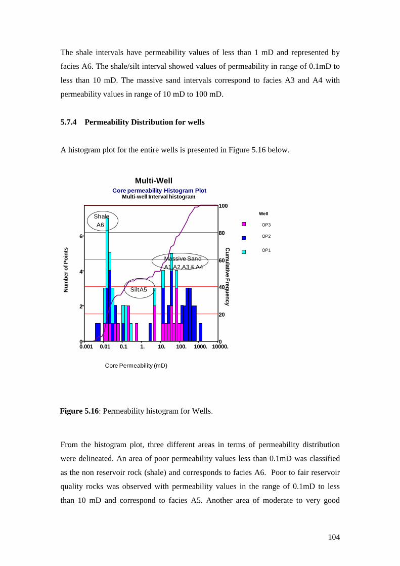
104

The shale intervals have permeability values of less than 1 mD and represented by

facies A6. The shale/silt interval showed values of permeability in range of 0.1mD to

less than 10 mD. The massive sand intervals correspond to facies A3 and A4 with

permeability values in range of 10 mD to 100 mD.

5.7.4 Permeability Distribution for wells

A histogram plot for the entire wells is presented in Figure 5.16 below.

Multi-Well

Core permeability Histogram PlotMulti-well Interval histogram

0

20

40

60

80

100

Cu

mu

lativ

e F

req

uen

cy

0.001 0.01 0.1 1. 10. 100. 1000. 10000.0

2

4

6

Nu

mb

er

of P

oin

ts

Well

OP3

OP2

OP1

Shale

Massive Sand

A6

Silt A5

A1,A2,A3 & A4


From the histogram plot, three different areas in terms of permeability distribution

were delineated. An area of poor permeability values less than 0.1mD was classified

as the non reservoir rock (shale) and corresponds to facies A6. Poor to fair reservoir

quality rocks was observed with permeability values in the range of 0.1mD to less

than 10 mD and correspond to facies A5. Another area of moderate to very good

Figure 5.16: Permeability histogram for Wells.

105

permeability values greater than mD was also delineated in the permeability plot and

represents the massive sandstone interval that corresponds to facies A1, A2, A3 and

A4 respectively.

This massive sandstone interval was regarded as the best reservoir rock in terms of

permeability distribution.

Well OP2 dominate the good permeability area while well OP1 dominates the poor

permeability area. The modal class was noticed at permeability value of 0.01 mD

centred on well OP1 and OP2.

The distribution of permeability for all the well investigated showed that good

reservoir rocks and best facies are located at the top of the reservoirs and the poor

permeability were observed to be predominant in the lower part of the reservoirs and

consists of facies A5 and A6.

5.8 Interpretation of Fluid Saturation

The saturation of a formation is regarded as the fraction of its pore volume occupied

by the fluid. The symbol used for saturation is S and various subscripts are used to

represent saturation of different fluids. In this study the symbol used to represent

water saturation is Sw. Oil saturation is So, Gas saturation is Sg, and hydrocarbon

saturation is Sh.

The summation of all saturations in a given rock must equal 100 %, and water

saturation of a formation can vary from 100% to much smaller percentage but will

never be zero because there is always a small amount of capillary water or irreducible

water that cannot be displaced. Also for an oil or gas bearing reservoir rock, all the

hydrocarbon saturation cannot be removed or displaced, some of the oil or gases

remain trapped in the pore volume and this hydrocarbon saturation is regarded as

residual oil saturation.

The fluid saturation was determined by using the plug-end trims of the core plug The

method used involves using both heat and organic solvent to extract the pore fluids

and is called Dean-Stark extraction.

106

5.8.1 Well OP1 Fluid Saturation

Three types of fluid saturation values (saturation of gas, Sg, Saturation of oil So, and

saturation of water Sw) were reported in well OP1. The average saturation of water

(Sw) measured was 57 %; gas saturation (Sg) of 38 % and oil saturation of

approximately 5 % was measured as presented in Figure 5.17 below.

OP1

Well OP1 Fluid Saturation versus Depth Plot

0. 20. 40. 60. 80. 100.

Fluid Saturation (%)

3382.

3378.

3374.

3370.

3366.

3362.

De

pth

(m

)

Water Gas Oil

OP1Scale : 1 : 200


1

DEPTH

(M)

GammaRay

GRn (GAPI)0. 200.

LithoFacies


Porosity




ILD (OHMM)0.2 2000.



3375

Facies A3

Facies A4

Facies A5

Facies A4

Facies A6

3380

Sand

Stones.

Sand/silt

shaleA6

A3 & A4

A5

Figure 5.17: Well OP1 fluid saturation versus depth plot.

The plot of fluid saturation versus depth present an interval of increasing hydrocarbon

saturation at depth 3370 m to 3373 m which corresponds to facies A3 and A4. The

presence of decreasing water in this interval may represent irreducible water

107

saturation. Below this interval at facies A4, the water and hydrocarbon saturation was

constant to a depth of about 3378m which suspected to be the transition zone. The

water saturation tends to increase with a decrease in gas saturation at depth 3376m

which correspond to facies A6.

5.8.2 Well OP3 Fluid Saturation

In core 1 of well OP3, the fluid saturations reported were water saturation (Sw) with

an average value of 62 % and gas saturation of an average value of 38 %. No oil

saturation was observed in this interval. At depth of 3236.5m to 3238m (Figure 5.18a)

below, a decrease in water saturation was noticed from 60 % to about 40 %, while the

gas saturation at this interval increases from 40 % to 60 % and correspond to facies

A3 and A4. Sample for fluid saturation determination was not performed on facies

A5. At measured depth of 3242 m (facies A6), gas and water saturation were observed

at 18 % and 84 % respectively.

Figure 5.18a: Well OP3 core 1 fluid saturation versus depth plot.

Well OP3Core 1 Fluid Saturation versus Depth Plot

0. 20. 40. 60. 80. 100.Fluid Saturation (%)

3245.

3241.

3237.

3233.

3229.

3225.

De

pth

(m

)

A3 & A4

A6

Water Gas

OP3Scale : 1 : 150


1

DEPTH

(M)

GammaRay

GRn (GAPI)0. 150.

Lithofacies


Porosity


Ob Porosity ()0.5 0.


ILD (OHMM)0.2 2000.

MSFLC (OHMM)0.2 2000.

Cor Klin ()0.001 1000.

Facies A3

Facies A4

Facies A5

Facies A6

3240

3230

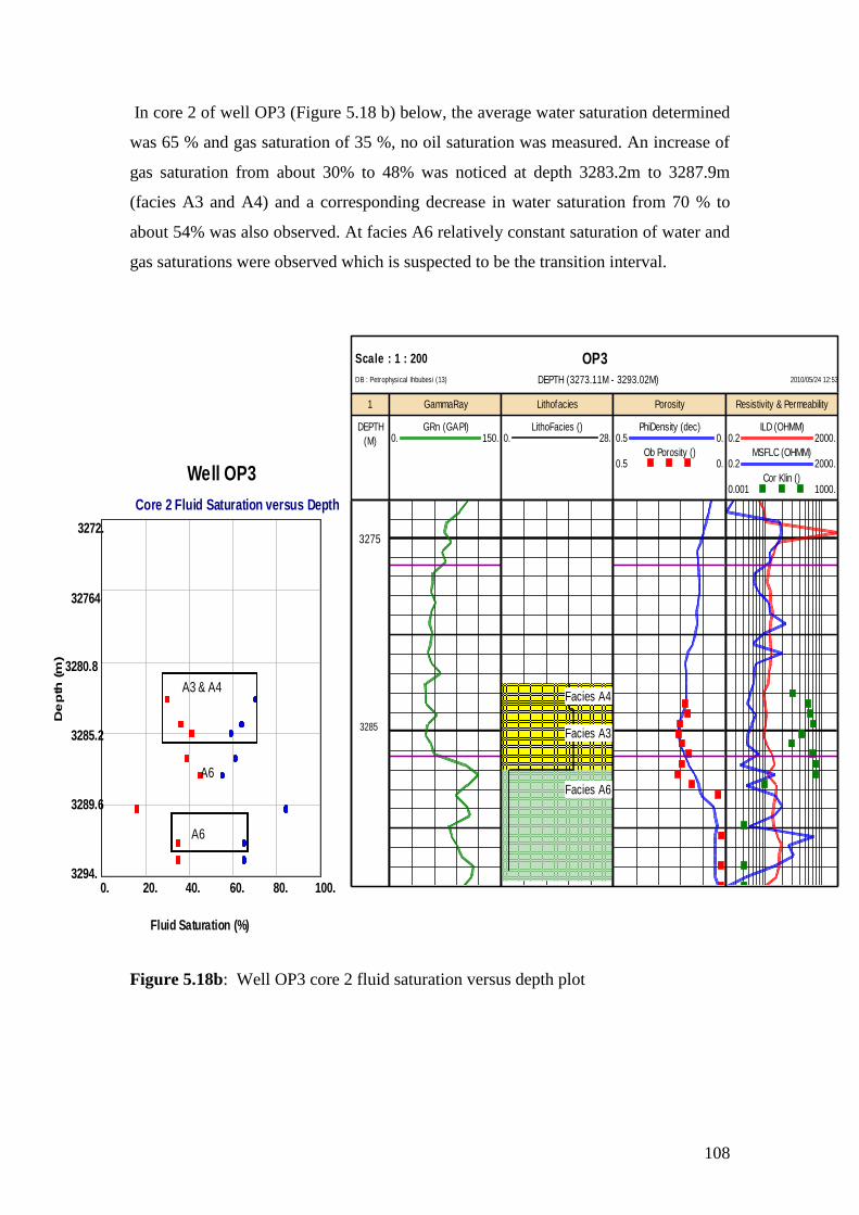
108

In core 2 of well OP3 (Figure 5.18 b) below, the average water saturation determined

was 65 % and gas saturation of 35 %, no oil saturation was measured. An increase of

gas saturation from about 30% to 48% was noticed at depth 3283.2m to 3287.9m

(facies A3 and A4) and a corresponding decrease in water saturation from 70 % to

about 54% was also observed. At facies A6 relatively constant saturation of water and

gas saturations were observed which is suspected to be the transition interval.

Figure 5.18b: Well OP3 core 2 fluid saturation versus depth plot

Well OP3

Core 2 Fluid Saturation versus Depth

0. 20. 40. 60. 80. 100.

Fluid Saturation (%)

3294.

3289.6

3285.2

3280.8

32764

3272.

De

pth

(m

)

A3 & A4

A6

A6

OP3Scale : 1 : 200


1

DEPTH

(M)

GammaRay

GRn (GAPI)0. 150.

Lithofacies


Porosity




ILD (OHMM)0.2 2000.


Cor Klin ()0.001 1000.

3275

Facies A3

Facies A4

Facies A5

Facies A6

Facies A4

Facies A3

Facies A6

3285

109

5.9 Comparison of Porosity- Permeability and Facies Distribution

The porosity-permeability cross plots are used to distinguish between rock types and

also show the trend between porosity and permeability. Porosity-permeability and

facies relationships vary from exploration well to well. The Klinkenberg Permeability

measured in mD is plotted on a logarithmic scale (y-axis) versus the porosity

measured as fraction is plotted on a linear scale (x-axis), and facies were assigned

linear values based on description were plotted on the (z-axis).The purpose of the z-

plot is to show the distribution of four variables (porosity, permeability, facies and

GR) instead of two (porosity and permeability).

Composition and abundance of principal framework grains have a great impact on

diagenetic processes controlling porosity reduction, preservation and enhancement

with burial. Heterogeneity and facies variations such as the vertical and lateral

changes from cross-bedded to ripple-laminated sandstone, affect reservoir

performance.

5.9.1 Porosity-Permeability and facies Distribution for well OP1

The core permeability was plotted in log scale on the y-axis against the core porosity

in linear scale on the x-axis, and facies and gamma ray on the z-axis as shown in

Figure 5.19 below.

Figure 5.19: Porosity-Permeability and gamma ray log and facies plot for well OP1

LogK(air) =-3.0412+25.6441*Phic

R2=0.89

Well OP1

Porosity-Permeability Plot

0. 0.06 0.12 0.18 0.24 0.3Core Porosity (v/v)

0.001

0.01

0.1

1.

10.

100.

1000.

Co

re P

erm

eab

ilit

y (

mD

)

A6

A5

A4

A3

A2

A1

0.

6.Facies

Log (Kair) = -3.0412 + 25.6241 * Porosity

R2= 0.8931

Well OP1

Porosity-Permeability and GR Plot

0. 0.06 0.12 0.18 0.24 0.3Core Porosity (v/v)

0.001

0.01

0.1

1.

10.

100.

1000.

Co

re P

erm

eab

ilit

y (

mD

)

Clean Sand

Shaly Sands

Shaly

Shale

0.

150.GR(API)

R2= 0.8931

Facies

A6

A4

A5A4

Facies

A6

110

The gamma ray log plot on the z-axis with values of 0 to 37 API represents clean

sandstone, 37.5 to 75 API as shaly sandstones, and 76 to 150 API as shale.

Three facies were observed, facies A4, A5 and A6 on the cross-plot of this well.

Facies A6 falls within gamma ray values of 75 to 150 API, with permeability values

of less than 1 mD and porosity values of less than 10%. This facies is recognized as

predominantly clay/siltstone and was classified as non reservoir rock. Facies A5 with

gamma ray value between 40 and 75 API was regarded as shaly sand formation which

posses a permeability value of slightly less than 10 mD and porosity value of about 13

%. Facies A4 is also regarded as a shaly sand formation based on the gamma ray

values that it represents. The permeability values are poor to good and porosity values

are above 10%.

Porosity permeability relationship of the interval is good with correlation coefficient

of R2= 0.8931 .The following relationship was established from the regression analysis

plot:

R2= 0.8931

Where:

K= Permeability (mD)

R = Correlation coefficient

5.9.2 Porosity-Permeability and Facies Distribution for well OP2

The cross plot of porosity-permeability and facies GR of well OP2 is presented in

Figure 5.20 below.

Log (K) = -3.1626 + 24.8170 * Core Porosity ………… (5.1)

111

Figure 5.20: Porosity-Permeability and facies and GR plot for well OP2

The plot shows three different data clustering points of different rock types and facies.

Facies A6 is of low porosity and permeability and is made up of GR values greater

than 76 API and could be interpreted as silt/shale to shaly formation .The other data

clustering point is composed of facies A5 and A4 having predominantly GR values

between 37.5 to 75 API values which represents shaly-silt formation with high

porosity and moderate permeability values.

Facies A1, A2 and A3 are made up of data clustering of high porosity and very good

permeability values and a GR values below 75 API which is predominantly of clean

sand formation and slight intercalation of shaly sand formation.

An empirical relationship between measured porosity and permeability was derived

using the following linear regression analysis:

K = 10(21.6648 * Porosity -2.687)

………………………… (5.2)

R2 =0.9379

Where:


R = Correlation Coefficient

Well OP2

Porosity-Permeability and Facies Plot

0. 0.06 0.12 0.18 0.24 0.3Core Porosity (v/v)

0.001

0.01

0.1

1.

10.

100.

1000.

10000.

Co

re P

erm

eab

ilit

y (

mD

)

A6

A5

A4

A3

A2

A1

0.

6.Facies


R2= 0.9379

Facies

A6 & A5

A1,A2 &

A3

A4

Well OP2

Porosity-permeability and GR Plot

0. 0.06 0.12 0.18 0.24 0.3Core Porosity (v/v)

0.001

0.01

0.1

1.

10.

100.

1000.

10000.

Co

re P

erm

eab

ilit

y (

mD

)

Clean Sand

Shaly Sands

Shaly

Shale

0.

150.GR(API)

R2= 0.9379Facies

A1,A2,A3

Facies

A5 & A6

A4

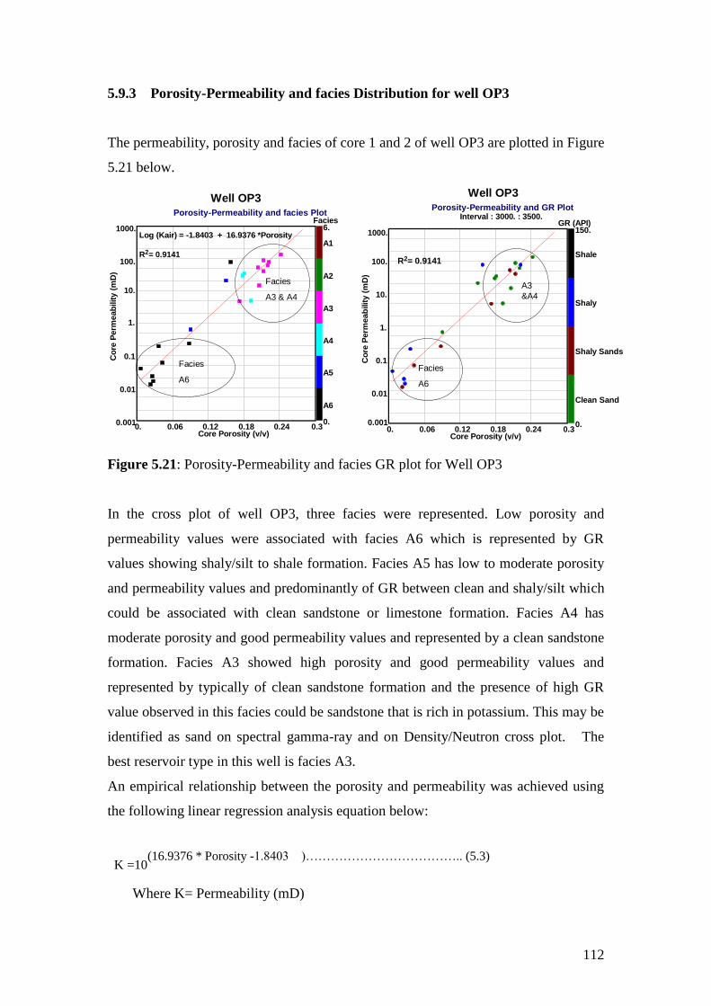
112

5.9.3 Porosity-Permeability and facies Distribution for well OP3

The permeability, porosity and facies of core 1 and 2 of well OP3 are plotted in Figure

5.21 below.

Figure 5.21: Porosity-Permeability and facies GR plot for Well OP3

In the cross plot of well OP3, three facies were represented. Low porosity and

permeability values were associated with facies A6 which is represented by GR

values showing shaly/silt to shale formation. Facies A5 has low to moderate porosity

and permeability values and predominantly of GR between clean and shaly/silt which

could be associated with clean sandstone or limestone formation. Facies A4 has

moderate porosity and good permeability values and represented by a clean sandstone

formation. Facies A3 showed high porosity and good permeability values and

represented by typically of clean sandstone formation and the presence of high GR

value observed in this facies could be sandstone that is rich in potassium. This may be

identified as sand on spectral gamma-ray and on Density/Neutron cross plot. The

best reservoir type in this well is facies A3.

An empirical relationship between the porosity and permeability was achieved using

the following linear regression analysis equation below:

K =10(16.9376 * Porosity -1.8403 )……………………………….. (5.3)

Where K= Permeability (mD)

Well OP3

Porosity-Permeability and facies Plot

0. 0.06 0.12 0.18 0.24 0.3Core Porosity (v/v)

0.001

0.01

0.1

1.

10.

100.

1000.

Co

re P

erm

eab

ilit

y (

mD

)

A6

A5

A4

A3

A2

A1

0.

6.Facies

Log (Kair) = -1.8403 + 16.9376 *Porosity

R2= 0.9141R2= 0.9141

Well OP3

Porosity-Permeability and GR PlotInterval : 3000. : 3500.

0. 0.06 0.12 0.18 0.24 0.3Core Porosity (v/v)

0.001

0.01

0.1

1.

10.

100.

1000.

Co

re P

erm

eab

ilit

y (

mD

)

Clean Sand

Shaly Sands

Shaly

Shale

0.

150.GR (API)

R2= 0.9141

Facies

A6

Facies

A3 & A4

Facies

A6

A3

&A4

113

5.9.4 Comparison of Porosity, Permeability and Facies for all wells

In order to determine a relationship between porosity-permeability and identify facies

that will contribute to flow of hydrocarbon of the study area, the porosity-permeability

and facies were plotted (Figure 5.22) below. The relationship established from the

cross plot will also serves as the field permeability predictor in un-cored intervals and

for Wells without core.

Figure 5.22: Porosity-permeability and facies distribution for wells

The facies A6 in the cross plot are predominant in the low porosity (porosity less than

10 %) and poor permeability (less than 1 mD) plot area coloured black which

represent shale formation. Facies A5 in the cross plot showed area of poor to fair

permeability and low to high porosity values. This facies fall between the low

porosity-permeability and high porosity-permeability interval and represent

sandstones and shaly- sands as compared with the GR plot. Sediments in this interval

may be intercalation of clean sandstone, siltstone and claystones.

Facies A4 and A3 are closely related having permeability values of moderate to good

and porosity values above 12 %. The high values recorded in this area may be due to

sandstone represented by GR clean sands which are moderately sorted grains and the

All Well


0. 0.06 0.12 0.18 0.24 0.3Core Porosity (v/v)

0.001

0.01

0.1

1.

10.

100.

1000.

10000.

Co

re P

erm

eab

ilit

y (

mD

)

A6

A5

A4

A3

A2

A1

0.

6.Facies


R2= 0.9201

All Well

Porosity-Permeability and GR PlotMulti well Interval plot

0. 0.06 0.12 0.18 0.24 0.3Core Porosity (v/v)

0.001

0.01

0.1

1.

10.

100.

1000.C

ore

Perm

eab

ilit

y (

mD

)

Clean Sand

Shaly Sands

Shaly

Shale

0.

150.GR (API)

Well

OP1

OP2

OP3

A5 & A6

A1 &A2

A3 & A4

A5 & A6

A3&A4

A1 &

A2R2= 0.9201

114

low values may be due to the shaly sands as predominantly represented by GR shaly

formation.

Facies A2 and A1 were observed to have the best reservoir rock quality with porosity

of higher than 18 % and good to very good permeability values and predominantly

represented by GR of clean sandstone and few shaly-sands. The sediments in this

facies are well sorted grains.

It is evident that a linear porosity-permeability relationship exists and a permeability

predictor could easily be constructed by means of a simple linear regression. An

empirical relationship was derived from the cross plot as given below:

K = 10 (20.8917 * Porosity -2.4284)

……………………………………… (5.4)

R2 = 0.9201

Where K = Permeability (mD)

Porosity = Porosity (v/v)

R= Correlation Coefficient

The equation 5.4 above shows a correlation coefficient of 0.92 which is very good

from statistical point of view and thus can be used provisionally to estimate

permeability provided the porosity is known either from log for other wells that do not

have core data . An accurate method will be used later in the study to determine the

values of permeabilities. From this analysis, it was observed that for one particular

value of porosity and permeability, it can be represented by different facies.

The low values of porosity and permeability values recorded may be due to the poorly

sorted sediments, the finer grained material tends to block the pore throats giving

decrease in permeability. Porosity is independent of grain size but decreases with

decreasing sorting while permeability depends on both grain size and sorting.

5.10 SPECIAL CORE ANALYSIS (SCAL)

The special core analysis are measurements made on core plugs that complements

conventional analysis measurements which are concern with measurements of

reservoir properties that allows calculation of static fluid distribution and dynamic

flow performance of a reservoir.

115

In this section, discussions will be focused on results of special core analysis

measurement ( SCAL) analyses on core plug samples from well OP1, OP2 and OP3

that were undertaken by Core Laboratories on behalf of South African Oil Exploration

(Pty) limited (PASA report, 1993) to determine the following:

Additional Routine analysis of Permeability to air, Klinkenberg corrected

permeability to air, and helium injection porosity and grain density at room

conditions.

Formation Resistivity Factor (FRF) at room conditions and as a function of

overburden pressure.

Formation Resistivity Index (RI) at room conditions

Capillary pressure measurements – Air-Brine porous plate cell and mercury

injection methods.

The special core analysis overburden measurements are laboratory measurements of

petrophysical properties aimed at determining the exact values under stress, pressure

and temperature conditions. The laboratory overburden pressure tests stimulate the net

overburden pressure which is the difference between the overburden pressure caused

by the weight of sediments and the reservoir pressure.

SCAL measurements are performed on a relatively small number of representative

samples and analysis can be performed at reservoir conditions using fluid samples.

5.10.1 Porosity, Permeability and Grain density Measurements

The permeability to air and porosity data obtained for each core sample after the

cleaning and drying processes help in sample selections for other SCAL tests because

it defines a minimum values for samples to meet before been utilized for other

analyses. Results of two wells OP1 and OP3 are presented below.

5.10.1.1 Well OP1 Porosity, Permeability and Grain density Measurements

In well OP1, six (6) samples were selected for SCAL analyses but following air

permeability and helium porosity measurements, two samples at depth 3372.93 and

3373.8 were found to be below test limits therefore was not suitable for further

testing.

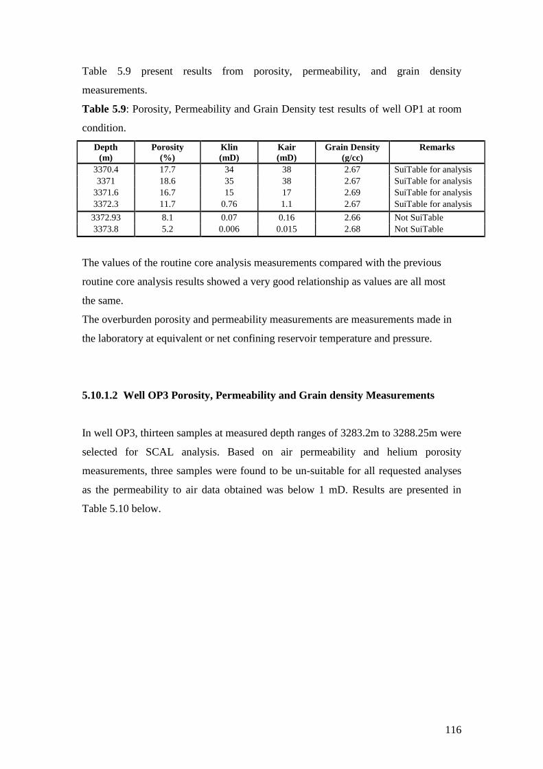
116

Table 5.9 present results from porosity, permeability, and grain density

measurements.

Table 5.9: Porosity, Permeability and Grain Density test results of well OP1 at room

condition.

Depth

(m)

Porosity

(%)

Klin

(mD)

Kair

(mD)

Grain Density

(g/cc)

Remarks

3370.4 17.7 34 38 2.67 SuiTable for analysis

3371 18.6 35 38 2.67 SuiTable for analysis

3371.6 16.7 15 17 2.69 SuiTable for analysis

3372.3 11.7 0.76 1.1 2.67 SuiTable for analysis

3372.93 8.1 0.07 0.16 2.66 Not SuiTable

3373.8 5.2 0.006 0.015 2.68 Not SuiTable

The values of the routine core analysis measurements compared with the previous

routine core analysis results showed a very good relationship as values are all most

the same.

The overburden porosity and permeability measurements are measurements made in

the laboratory at equivalent or net confining reservoir temperature and pressure.

5.10.1.2 Well OP3 Porosity, Permeability and Grain density Measurements

In well OP3, thirteen samples at measured depth ranges of 3283.2m to 3288.25m were

selected for SCAL analysis. Based on air permeability and helium porosity

measurements, three samples were found to be un-suitable for all requested analyses

as the permeability to air data obtained was below 1 mD. Results are presented in

Table 5.10 below.

117

Table 5.10: Porosity, permeability and grain density test results of well OP3 at room

condition.

Depth

(m)

Porosity

(%)

Klin

(mD)

Kair

(mD)

Grain Density

(g/cc)

Remarks

3283.2 20.2 4.5 6 2.71 Suitable for analysis

3283.4 18.7 3.3 4.4 2.71 Suitable for analysis

3283.5 17.7 2.5 3.5 2.7 Suitable for analysis

3284.74 23.5 70 80 2.7 Suitable for analysis





3287 24.3 69 79 2.69 Suitable for analysis


3288.09 9.5 0.06 0.14 2.68 Not Suitable

3288.15 6.8 0.03 0.06 2.67 Not Suitable

3288.25 6.1 0.02 0.04 2.68 Not Suitable

5.10.2 Formation Resistivity Factor (FRF) Measurements

The formation resistivity factor (FRF) is defined as the ratio of resistivity of the 100

percent water saturated rock sample to the water resistivity. It is a function of porosity

and pore geometry of rock.

The core plugs used in this measurement were first cleaned dry plugs and later

evacuated and pressure saturated with simulated formation brine. Electrical resistance

of the brine saturated core plugs were measured at room conditions on consecutive

days until results stabilized indicating ionic equilibrium within the core plugs.

The formation brine used in this study consists of sodium chloride (NaCl) and calcium

chloride (CaCl2). The calcium chloride was used to minimise any possible reactive

clay problems. The formation resistivity values were determined at ambient condition

for 100 percent brine saturated samples and also simulated to net overburden pressure

which will be presented later.

The cementation exponent (m) which is a very useful parameter for the determination

of water saturation is calculated from the slope of plotting measured values of FRF

against porosity setting the intercept „”a” to unity.

118

5.10.2.1 Formation Resistivity Factor (FRF) measurement Results for well OP1

The FRF measurement for well OP1 was performed at temperature of 77 oF which is

equivalent to 25oC and the brine resistivity of 0.32 Ohm-m was used at room

condition. The brine used consisted of approximately 18,500 ppm of dissolved solids

consisting of 80 % sodium chloride (NaCl) and 20 % calcium chloride (CaCl2).

The result of formation resistivity factor (FRF) performed on four samples of well

OP1 is presented in Table 5.11 below.

Table 5.11: Result of well OP1 FRF measurement at room condition

The room condition as used means measurements made at surface atmospheric

condition at 25 oC or 77

oF

5.10.2.2 Formation Resistivity Factor (FRF) measurement Results for well OP3

The formation resistivity measurement for well OP3 was performed at room condition

at a temperature of 77 oF and overburden condition. The resistivity of brine used was

0.13 Ohm-m. The water composition was confirmed with the Schlumberger log

interpretation chart Gen-9.

The total dissolved solids were 51.282 mg/l and constituents were sodium chloride

(NaCl) having 41.026 mg/l and calcium chloride 10.256 mg/l. Shown in Table 5.12 is

results obtained from FRF measurements.

Depth

(m)

Porosity (%)

Room Condition

FRF

Room Condition

3370.40 17.7 25.47

3371.00 18.6 24.63

3371.60 16.7 30.38

3372.30 11.7 54.49

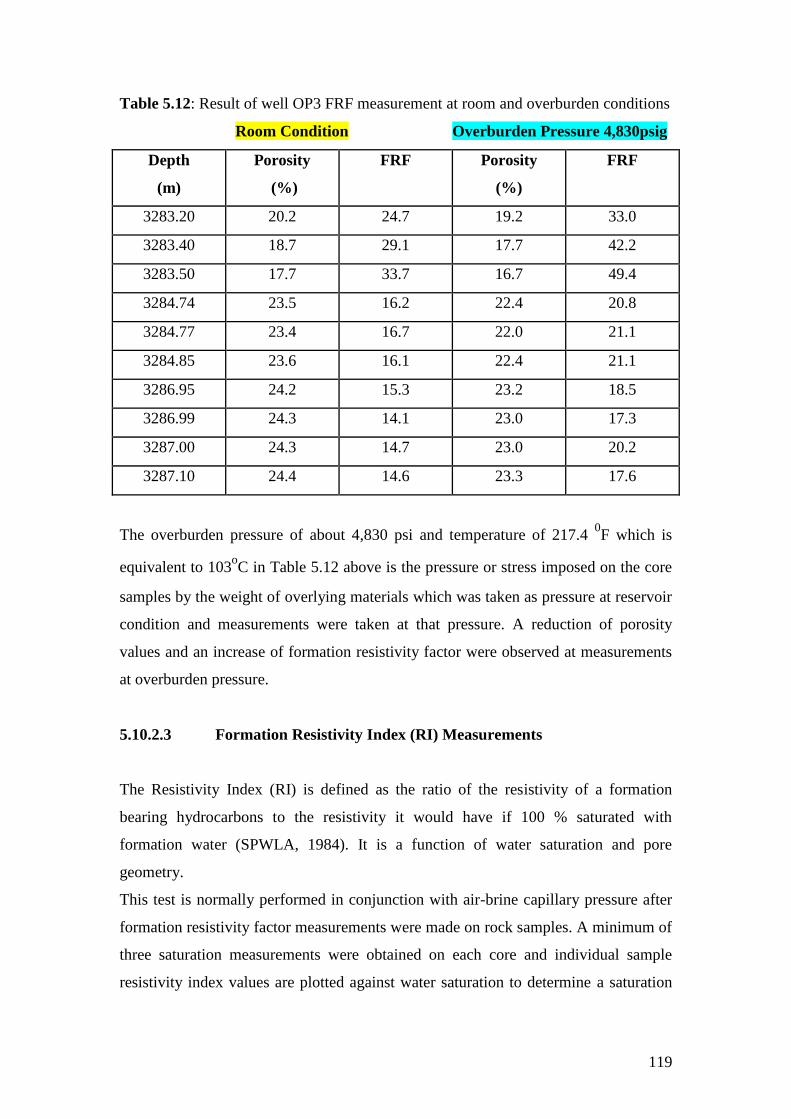
119

Table 5.12: Result of well OP3 FRF measurement at room and overburden conditions

Room Condition Overburden Pressure 4,830psig

Depth

(m)

Porosity

(%)

FRF Porosity

(%)

FRF

3283.20 20.2 24.7 19.2 33.0

3283.40 18.7 29.1 17.7 42.2

3283.50 17.7 33.7 16.7 49.4

3284.74 23.5 16.2 22.4 20.8

3284.77 23.4 16.7 22.0 21.1

3284.85 23.6 16.1 22.4 21.1

3286.95 24.2 15.3 23.2 18.5

3286.99 24.3 14.1 23.0 17.3

3287.00 24.3 14.7 23.0 20.2

3287.10 24.4 14.6 23.3 17.6

The overburden pressure of about 4,830 psi and temperature of 217.4 0F which is

equivalent to 103oC in Table 5.12 above is the pressure or stress imposed on the core

samples by the weight of overlying materials which was taken as pressure at reservoir

condition and measurements were taken at that pressure. A reduction of porosity

values and an increase of formation resistivity factor were observed at measurements

at overburden pressure.

5.10.2.3 Formation Resistivity Index (RI) Measurements

The Resistivity Index (RI) is defined as the ratio of the resistivity of a formation

bearing hydrocarbons to the resistivity it would have if 100 % saturated with

formation water (SPWLA, 1984). It is a function of water saturation and pore

geometry.

This test is normally performed in conjunction with air-brine capillary pressure after

formation resistivity factor measurements were made on rock samples. A minimum of

three saturation measurements were obtained on each core and individual sample

resistivity index values are plotted against water saturation to determine a saturation

120

exponent (n) which is a slope of a line relating saturation and resistivity index (Core

laboratory, 1982).

These measurements were performed in the Albian age reservoir sections of two wells

(OP1 and OP3) in the study area. The results from resistivity index measurements are

presented.

5.10.3.1 Formation Resistivity Index Results for well OP1

In well OP1, formation resistivity index measurements were conducted on four

samples at room condition as presented in Table 5.13. About six different resistivity

index measurements were performed on each sample at different brine saturations.

Table 5.13: Resistivity Index results for well OP1

Depth

(m)

Brine Saturation

(%)

Resistivity Index

(RI)

3370.4 91 71 57 52 50 46 43 1.1 1.6 2.2 2.4 2.9 3.1 3.4

3371 64 51 48 45 42 40 1.9 2.8 3 3.5 3.7 4

3371.6 75 56 51 48 45 42 1.5 2.4 2.8 3.3 3.5 3.7

3372.3 71 64 57 52 1.6 1.9 2.1 2.3

5.10.3.2 Formation Resistivity Index Results for Well OP3

In well OP3, formation resistivity index measurements were performed on ten

samples at different brine saturation percent pore spaces as shown in Table 5.14.

Table 5.14: Resistivity Index results for well OP3

Depth

(m)

Brine Saturation

( % ) Resistivity Index

(RI)

3283.2 100 71.4 63.2 53.3 50 1 1.98 2.41 2.91 3.27

3283.4 100 71.2 62.7 55.7 52.1 1 2.1 2.34 2.57 3.3

3283.5 100 72.8 63.5 55.9 51.6 1 2.23 2.53 3.06 3.44

3284.74 100 54.9 48.1 40.3 37.9 1 2.11 2.71 4.3 6

3284.77 100 57.6 50.5 41.2 38 1 1.85 2.92 3.79 5.5

3284.85 100 55.2 49.7 40.9 37.4 1 2.07 3.18 5.27 6.13

3286.95 100 56 49 41.8 36.3 1 2.12 3.01 4.07 6.3

3286.99 100 52.4 45.5 37.3 33 1 2.57 3.85 4.91 8.43

3287 100 50.7 44.4 35.9 32.5 1 2.64 3.78 4.97 8.3

3287.1 100 50.4 44.2 35.7 32.4 1 1.59 3.21 5.05 8.18

121

5.10.4 Interpretation of Results

5.10.4.1 Porosity Overburden Correction

When the core is brought to the surface, all confining forces are removed and the rock

tends to expand in all directions. This expansion causes a modification of the pore

geometry which may impact on the rock permeability and porosity depending on

pressure differential, the consolidation state of the rock and clay content. Discrepancy

between laboratory and in situ measurements is due the increase in volume that occurs

when the core is brought to a lower pressure and temperature at the surface because of

the removal of overlying sediment column (Moran, 1995).

Overburden correction is regarded as the correction from laboratory condition

measurements to net effective overburden stress at in situ reservoir conditions. This

correction is carried out because routine core analysis measurements may incorporate

systematic errors because these values are measured at low pressure which may lead

to an over estimation.

An overburden correction should always be applied to the routine core data. When

overburden measurements are available, a correction function for the routine data can

be constructed otherwise empirical relationships can be applied (Luca & Jean-Claude,

2001).

In this study, the overburden corrections were applied to routine core porosity values

due to the availability of porosity measurement data at overburden pressure. An

empirical relationship between porosity at overburden and ambient conditions is

established for porosity overburden corrections. No special core analysis

measurements of permeability values at overburden equivalent or net confining

pressures were recorded; therefore no permeability overburden corrections will be

applied to the routine core analysis permeabilities.

The special core analysis data of well OP3 at room and overburden pressure

conditions provide data for this correction. The overburden corrected porosity values

will be used to calibrate wireline log porosity measurements. Table 5.15 present data

for overburden correction.

122

Table 5.15: Well OP3 core 2 data used for porosity overburden correction.

Depth

(m)

Porosity

(%)

Room condition

Porosity

(%)

overburden pressure

3283.20 20.2 19.2

3283.40 18.7 17.7

3283.50 17.7 16.7

3284.74 23.5 22.4

3284.77 23.4 22.0

3284.85 23.6 22.4

3286.95 24.2 23.2

3286.99 24.3 23.0

3287.00 24.3 23.0

3287.10 24.4 23.3

The porosity at overburden pressure (4,830 psi) was plotted against porosity values at

room condition on a linear scale as shown in Figure 5.23a below.

Well OP3

Overburden Porosity Vs Room Condition Porosity

0.01 0.068 0.126 0.184 0.242 0.3Porosity at Room Condition (v/v)

0.

0.06

0.12

0.18

0.24

0.3

Po

rosit

y a

t 4,8

30 p

si O

verb

urd

en

Co

nd

itio

n (v/v

)

A6

A5

A4

A3

A2

A1

0.

6.Facies

Y=0.9651 * Poro -0.3577

R2= 1.0000

Figure 5.23a: Well OP3 porosity at overburden pressure versus porosity at room

condition

123

To obtain an empirical linear relationship for the application of porosity overburden

corrections, the regression equation from the plot of porosity at overburden pressure

against porosity at room condition is used as given in the equation below:

Φ correct = 0.9651 (Φ routine) - 0.3577 .................................... (5.5)

Where:

Φ correct = Overburden corrected porosity

Φ routine = Routine core porosity

Another useful parameter is the Pore Volume Reduction Factor (PRF) which is

defined as the ratio of the overburden corrected porosity to routine core porosity. An

average porosity reduction factor of 0.95 was obtained. Adopting a mean PRF would

result in an over correction in higher porosity sections and under correction in the

lowest porosity sections, hence equation 4.6 above is used to correct the routine core

porosity measured at room conditions to in situ reservoir conditions.

The routine core porosity corrected values to the equivalent in situ reservoir

conditions are given in Table 5.16 below.

124

Table 5.16: Wells OP1, OP2 and OP3 calculated overburden corrected porosities

Well OP1 Well OP2 Well OP3

Depth

(m)

Routine

Porosity

(%)

Corrected

Porosity

(%) 3370.05 18.9 17.9

3370.6 20.2 19.1

3371.07 16.9 15.9

3371.4 16.4 15.5

3371.9 16.5 15.6

3372.03 12.7 11.9

3372.53 9.5 8.8

3378.98 6.9 6.3

3373.75 5.0 4.5

3375.6 3.0 2.5

3375.98 2.0 1.6

3376.62 7.7 7.1

3376.86 8.6 8.0

3377.12 10.1 9.4

3377.36 9.6 8.9

3377.54 7.0 6.4

3377.78 7.9 7.3

3378.23 9.2 8.5

3378.48 8.6 7.9

3378.58 7.6 7.0

3379.24 6.8 6.2

3379.64 1.2 0.8

3379.82 4.9 4.4

3380.15 3.3 2.8

Depth

(m)

Routine

Porosity

(%)

Corrected

Porosity

(%)

3446.20 23.06 21.9

3447.08 24.24 23.3

3447.11 24.17 23.0

3447.83 18.65 17.6

3448.69 22.01 20.9

3449.52 20.27 19.2

3450.58 22.32 21.2

3451.70 23.54 22.4

3452.14 23.83 22.6

3452.59 24.01 22.8

3453.68 23.03 21.9

3454.72 24.25 23.0

3455.08 22.96 21.8

3455.55 18.83 17.8

3455.86 10.42 9.7

3456.15 4.59 4.1

3456.65 3.37 2.9

3457.18 3.27 2.8

3457.74 21.39 20.3

3458.69 21.36 20.3

3459.59 20.11 19.0

3460.00 21.93 20.8

3460.10 22.05 20.9

3461.48 23.07 21.9

3462.54 18.91 17.9

3463.48 19.55 18.5

3464.59 8.19 7.5

3464.81 4.92 4.4

3465.40 2.95 2.5

3466.47 6.23 5.7

3466.75 4.43 3.9

3467.50 4.12 3.6

3467.60 3.89 3.4

3468.17 5.96 5.4

Depth

(m)

Routine

Porosity

(%)

Corrected

Porosity

(%) 3236.1 24.2 23.0

3236.35 22.6 21.5

3236.51 21.3 20.2

3236.81 21.4 20.3

3237.05 18.1 17.1

3237.26 18.1 17.1

3237.51 15.0 14.1

3237.77 12.9 12.1

3237.95 9.1 8.4

3238.3 8.9 8.2

3238.5 6.3 5.7

3238.52 8.8 8.1

3239.05 4.3 3.8

3243.6 0.6 0.2

3283.2 19.2 18.2

3283.6 17.8 16.8

3283.85 17.8 16.8

3284.1 20.4 19.3

3284.35 21.3 20.2

3284.45 22 20.9

3285.05 22.2 21.1

3285.3 22.8 21.6

3285.34 20.6 19.5

3285.83 17.3 16.3

3286.08 14.3 13.4

3286.3 20.4 19.3

3286.55 22.3 21.2

3286.6 22.2 21.1

3287.25 23.3 22.1

3287.3 15.8 14.9

3287.9 3.7 3.2

3290.06 2.3 1.9

3291.76 2.7 2.2

3292.79 2.6 2.2

125

5.10.5 Derivation of Cementation exponent From Formation Resistivity Factor

The cementation of a rock is defined as the process of deposition of dissolved mineral

components in the interstices of sediments. The process involves coming together of

sediment to form a new rock during diagenesis or lithification (Boggs, 2006).

The cementation exponent which is represented by “m”is a function of the shape and

distribution of pores and it is determined from the slope of the plot of the formation

resistivity factor versus the porosity. The degree of cementation of sand particles

depends on the nature and distribution of the cementing materials; less cemented

sandstones normally have higher porosity values and lower formation resistivity

factor values.

The value of the cementation exponent reflects the tortuosity of the interconnected

pore space and ranges between 1 and 2.3 (Luca, 2001). The more complex the current

path is, the higher the cementation exponent which implies higher value of “m”. The

cementation exponent plays a critical role in the determination of water saturation

calculations.

The typical values used in classification of cementation for rocks are given in the

Table below:

Table 5.17a: Classification of cementation exponent

Classification Cementation (-m) values

Highly Cemented 2.0 -2.2

Moderately Cemented 1.8 -1.9

Slightly cemented 1.6 -1.7

Very Slightly Cemented 1.4 -1.5

Not Cemented 1.30

(Pirson, 1958)

126

5.10.5.1 Well OP1 Cementation Exponent (m) at Room Condition

The cementation exponent m was derived from the slope of the cross plot of

formation resistivity factor versus porosity by setting the tortuosity “a” the intercept to

unity as shown in Figure 5.23b below for well OP1.

Well OP1

FRF Vs Porosity and Facies at Room Condition

0.01 0.02 0.05 0.1 0.2 0.5 1.

Porosity (v/v)

1.

2.

5.

10.

20.

50.

100.

Fo

rma

tio

n R

es

isti

vit

y F

ac

tor

(FR

F)

A6

A5

A4

A3

A2

A1

0.

6.

Facies

Slope=m=1.89

.FRF=1/Φ1.89

Figure 5.23b: Formation resistivity factor (FRF) vs porosity plot for Well OP1

The slope gives the cementation exponent (m) from the equation, FRF = 1 / Φm

.

The values of cementation exponent (m) are given in Table 5.17b below. The values

range from 1.80 to 1.9 with a mean value of 1.89.

Table 5.17b: Cementation exponent (m) from Formation resistivity factor

measurement

Depth

(m)

Porosity

(%)

FRF Cementation

exponent (-m)

3370.40 17.7 25.47 1.88

3371.00 18.6 24.63 1.90

3371.60 16.7 30.38 1.90

3372.30 11.7 54.49 1.87

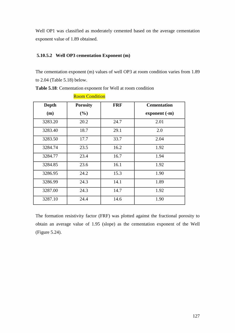
127

Well OP1 was classified as moderately cemented based on the average cementation

exponent value of 1.89 obtained.

5.10.5.2 Well OP3 cementation Exponent (m)

The cementation exponent (m) values of well OP3 at room condition varies from 1.89

to 2.04 (Table 5.18) below.

Table 5.18: Cementation exponent for Well at room condition

Room Condition

Depth

(m)

Porosity

(%)

FRF Cementation

exponent (-m)

3283.20 20.2 24.7 2.01

3283.40 18.7 29.1 2.0

3283.50 17.7 33.7 2.04

3284.74 23.5 16.2 1.92

3284.77 23.4 16.7 1.94

3284.85 23.6 16.1 1.92

3286.95 24.2 15.3 1.90

3286.99 24.3 14.1 1.89

3287.00 24.3 14.7 1.92

3287.10 24.4 14.6 1.90

The formation resistivity factor (FRF) was plotted against the fractional porosity to

obtain an average value of 1.95 (slope) as the cementation exponent of the Well

(Figure 5.24).

128

Well OP3

FRF Vs Porosity and Facies at Room Condition

0.01 0.02 0.05 0.1 0.2 0.5 1.

Porosity (v/v)

1.

2.

5.

10.

20.

50.

100.

Fo

rma

tio

n R

es

isti

vit

y f

ac

tor

(FR

F)

A6

A5

A4

A3

A2

A1

0.

6.

Facies

Slope=m=1.94

FRF=1/Φ1.94

Figure 5.24: Plot of Well OP3 formation resistivity factor versus fractional porosity

In this particular well, the cementation exponent was determined from two types of

facies (A4 and A5) within the interval measured at room conditions. Facies A4

showed higher formation resistivity factor values than facies A3. In terms of porosity,

facies A3 appeared to be more porous than facies A4 which indicate that facies A4 is

more cemented than facies A3. The cementation exponent determined in well OP3

was classified as moderately cemented having an average cementation value of 1.95.

5.10.5.3 Effect of Overburden Pressure on Cementation

The formation resistivity factor and porosity of well OP3 were measured at

overburden pressure of 4,830 psi, and cementation exponent values derived from the

cross plot of FRF vs. porosity varies from 1.94 to 2.17 with mean of 2.05 as shown in

Figure 5.25 below.

129

Figure 5.25: Formation resistivity factor versus porosity at overburden pressure

The cementation exponent values determined at overburden condition for well OP3

varies from 1.94 to 2.17 as shown in Table 5.19 below.

Table 5.19: Well OP3 cementation exponent at overburden pressure (4,830 psi)

Depth

(m)

Porosity

(%)

FRF Cementation

Exponent (-m)

3283.20 19.2 33.0 2.11

3283.40 17.7 42.2 2.17

3283.50 16.7 49.4 2.17

3284.74 22.4 20.8 2.03

3284.77 22.0 21.1 2.03

3284.85 22.4 21.1 2.03

3286.95 23.2 18.5 2.02

3286.99 23.0 17.3 1.94

3287.00 23.0 20.2 2.05

3287.10 23.3 17.6 1.98

Well OP3

FRF Vs Porosity at Overburden Condition

0.01 0.02 0.05 0.1 0.2 0.5 1.

Porosity (v/v)

1.

2.

5.

10.

20.

50.

100.

Fo

rma

tio

n R

es

isti

vit

y F

ac

tor

(FR

F)

A6

A5

A4

A3

A2

A1

0.

6.

Facies

Slope=m=

2.05FRF=1/Φ2.05

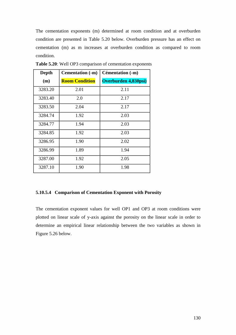
130

The cementation exponents (m) determined at room condition and at overburden

condition are presented in Table 5.20 below. Overburden pressure has an effect on

cementation (m) as m increases at overburden condition as compared to room

condition.

Table 5.20: Well OP3 comparison of cementation exponents

Depth

(m)

Cementation (-m)

Room Condition

Cémentation (-m)

Overburden 4,830psi)

3283.20 2.01 2.11

3283.40 2.0 2.17

3283.50 2.04 2.17

3284.74 1.92 2.03

3284.77 1.94 2.03

3284.85 1.92 2.03

3286.95 1.90 2.02

3286.99 1.89 1.94

3287.00 1.92 2.05

3287.10 1.90 1.98

5.10.5.4 Comparison of Cementation Exponent with Porosity

The cementation exponent values for well OP1 and OP3 at room conditions were

plotted on linear scale of y-axis against the porosity on the linear scale in order to

determine an empirical linear relationship between the two variables as shown in

Figure 5.26 below.

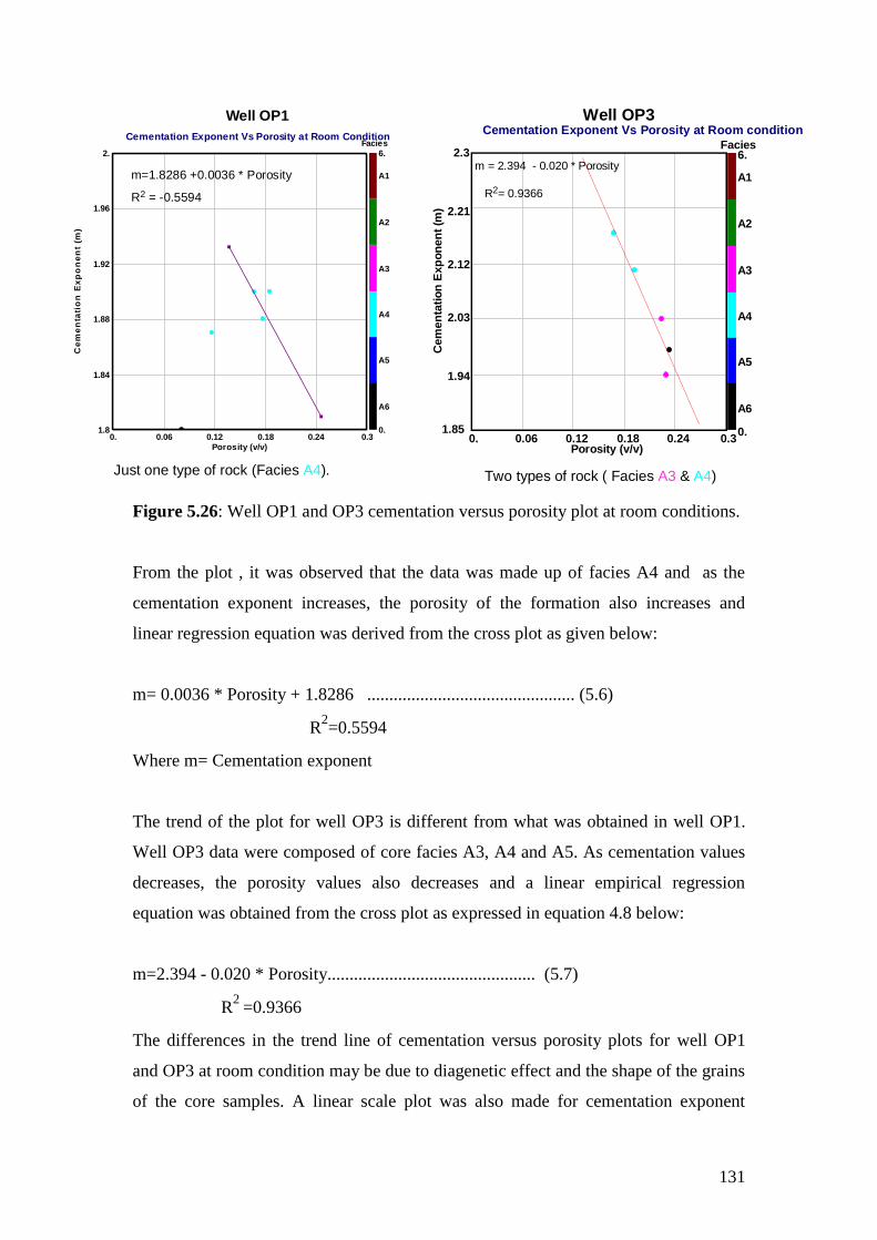
131

Figure 5.26: Well OP1 and OP3 cementation versus porosity plot at room conditions.

From the plot , it was observed that the data was made up of facies A4 and as the

cementation exponent increases, the porosity of the formation also increases and

linear regression equation was derived from the cross plot as given below:

m= 0.0036 * Porosity + 1.8286 ............................................... (5.6)

R2=0.5594

Where m= Cementation exponent

The trend of the plot for well OP3 is different from what was obtained in well OP1.

Well OP3 data were composed of core facies A3, A4 and A5. As cementation values

decreases, the porosity values also decreases and a linear empirical regression

equation was obtained from the cross plot as expressed in equation 4.8 below:

m=2.394 - 0.020 * Porosity............................................... (5.7)

R2

=0.9366

The differences in the trend line of cementation versus porosity plots for well OP1

and OP3 at room condition may be due to diagenetic effect and the shape of the grains

of the core samples. A linear scale plot was also made for cementation exponent

Well OP1

Cementation Exponent Vs Porosity at Room Condition

0. 0.06 0.12 0.18 0.24 0.3

Porosity (v/v)

1.8

1.84

1.88

1.92

1.96

2.

Ce

me

nta

tio

n E

xp

on

en

t (m

)

A6

A5

A4

A3

A2

A1

0.

6.

Facies

Just one type of rock (Facies A4).

Well OP3Cementation Exponent Vs Porosity at Room condition

0. 0.06 0.12 0.18 0.24 0.3Porosity (v/v)

1.85

1.94

2.03

2.12

2.21

2.3

Cem

en

tati

on

Exp

on

en

t (m

)

A6

A5

A4

A3

A2

A1

0.

6.Facies

m = 2.394 - 0.020 * Porosity

R2= 0.9366

m=1.8286 +0.0036 * Porosity

R2 = -0.5594

Two types of rock ( Facies A3 & A4)

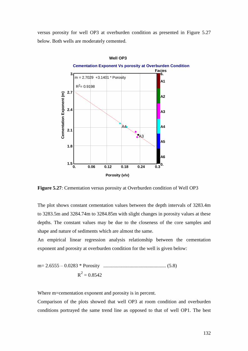
132

versus porosity for well OP3 at overburden condition as presented in Figure 5.27

below. Both wells are moderately cemented.

Figure 5.27: Cementation versus porosity at Overburden condition of Well OP3

The plot shows constant cementation values between the depth intervals of 3283.4m

to 3283.5m and 3284.74m to 3284.85m with slight changes in porosity values at these

depths. The constant values may be due to the closeness of the core samples and

shape and nature of sediments which are almost the same.

An empirical linear regression analysis relationship between the cementation

exponent and porosity at overburden condition for the well is given below:

m= 2.6555 – 0.0283 * Porosity .................................................. (5.8)

R2 = 0.8542

Where m=cementation exponent and porosity is in percent.

Comparison of the plots showed that well OP3 at room condition and overburden

conditions portrayed the same trend line as opposed to that of well OP1. The best

Well OP3

Cementation Exponent Vs porosity at Overburden Condition

0. 0.06 0.12 0.18 0.24 0.3

Porosity (v/v)

1.5

1.8

2.1

2.4

2.7

3.

Cem

en

tati

on

Exp

on

en

t (m

)

A6

A5

A4

A3

A2

A1

0.

6.Facies

m = 2.7029 +3.1401 * Porosity

R2= 0.9198

A4

A3

133

correlation coefficient was obtained from well OP3 cementation versus porosity plot

at room condition with value of about 0.94. Based on the number of data used for the

correlation and the higher correlation coefficient obtained from well OP3 at room

condition, therefore equation 5.8 above will be used for the evaluation.

5.10.5.5 Comparison of Cementation Exponent with Permeability

The cementation exponent plot on a linear scale against the permeability values on a

log scales for well OP1 and OP3 at room condition is presented in Figure 5.28 below.

Figure 5.28: Well OP1 and OP3 cementation exponent Vs permeability at room

temperature

The plot of Well OP1 was on core facies A4 and it showed that as cementation

increases, the permeability values tend to decrease and linear relationship between the

cementation exponents was obtained from the regression analysis as shown in the

equation below:

m= 0.0058*(log K) + 1.8782 ........................................................................... (5.9)

R2=0.4827

Where m= cementation exponent and K is the permeability in mD.

Well OP1

Cementation Exponent Vs permeability

0.01 0.1 1. 10. 100. 1000.

Permeability (mD)

1.82

1.856

1.892

1.928

1.964

2.

Ce

me

nta

tio

n E

xp

on

en

t (m

)

A6

A5

A4

A3

A2

A1

0.

6.

Facies

m=1.8514+0.0313 * log (k)

R2 = 0.8170

Well OP3Cementation Vs Permeability at Room Condition

0.001 0.01 0.1 1. 10. 100. 1000.Permeability (mD)

1.82

1.896

1.972

2.048

2.124

2.2

Cem

en

tati

on

Exp

on

en

t (m

)

A6

A5

A4

A3

A2

A1

0.

6.Facies

m = 2.2069 + 0.1202 * Log (K)

R2= 0.9226

134

A poor regression analysis value of 48% was obtained which implies that a poor

relationship exists between the plotted data and equation 5.9 could be used with

caution.

In well OP3, the permeability values decreases as the cementation increases as shown

in Figure 5.28 above and cementation also decreases as the depth increases. A good

relationship exists between the cementation exponent values and permeability as

shown in the regression coefficient value of about 94 % confidence.

The empirical relationship is given by the regression analysis below:

m=2.0597 – 0.035*(log K) ...................................................................... (5.10)

Where m is cementation exponent and K is permeability in mD.

Equation 5.10 above demonstrates a better relationship between cementation exponent

and permeability and hence could be used to estimate values of cementation exponent

provided permeability values are known.

It could be concluded that in well OP1, the slight increment in cementation observed

may be due to the closeness of the data and the core Facies A4, while in well OP3

cementation reduce porosity and permeability and the core facies were facies A3, A4

and A5.

5.10.6 Determination of Saturation Exponent (n)

The saturation exponent “n” is determined from the slope of a plot of resistivity index

on a lo-log scale versus the water saturation. The saturation exponent depends on rock

type and the way in which the pores are connected. The value of n is affected by

wettability, overburden pressure, type and amount of clay, and nature and distribution

of reservoir fluids (Djebbar, 1999).

135

5.10.6.1 Well OP1 Formation Resistivity Index (RI) versus Saturation at Room

Condition

The saturation exponent (n) of well OP1 was determined from the slope of resistivity

index versus water saturation as shown in Figure 5.29 below showing facies A4 as the

dominant facies in the interval plotted.

Figure 5.29: Well OP1 resistivity index versus water saturation plot.

The values of n vary from 1.43 to 1.53 with mean value of 1.45 as presented in Table

5.21.

Table 5.21: Well OP1 result of resistivity index measurements and n values

Depth

(m)

Brine Saturation

(%)

Resistivity index

(RI)

(-n)

3370.4 91 71 57 52 50 46 43 1.1 1.6 2.2 2.4 2.9 3.1 3.4 1.43

3371 64 51 48 45 42 40 - 1.9 2.8 3.0 3.5 3.7 4.0 - 1.51

3371.6 75 56 51 48 45 42 - 1.5 2.4 2.8 3.3 3.5 3.7 - 1.53

3372.3 71 64 57 52 1.6 1.9 2.1 2.3 1.34

Well OP1

Resistivity Index Vs Saturation

0.01 0.02 0.05 0.1 0.2 0.5 1.

Saturation (v/v)

1.

2.

5.

10.

Re

sis

tiv

ity

In

de

x (

RI)

A6

A5

A4

A3

A2

A1

0.

6.

Facies

RI = 1/Sw 1.45

Slope=n=1.45

Just one rock type (facies A4)

136

A plot of resistivity index versus saturation for well OP1 is given in Figure 5.29 above

and individual depth plots are in appendix C.

5.10.6.2 Well OP3 Saturation Exponent (n) Determination at Room Condition

The saturation exponent (n) was determined from the slope of plotting resistivity

index versus water saturation gives an average value of 1.94 as shown in Figure 5.30.

Facies A3 and A4 were observed at the interval plotted.

Figure 5.30: Well OP3 resistivity index versus saturation plot

The depth plots of “n” for this well are presented in appendix C. The n values vary

from 1.89 to 2.02 with an average value of 1.94 as indicated in Table 5.22 below.

Well OP3

Resistivity Index Vs Saturation at Room Condition

0.01 0.02 0.05 0.1 0.2 0.5 1.

Saturation (v/v)

1.

2.

5.

10.

Re

sis

tiv

ity

In

de

x (

RI)

A6

A5

A4

A3

A2

A1

0.

6.

Facies

RI = 1/Sw 1.94

Slope=n=1.94

Two reservoir rock types (facies A3 and A4)

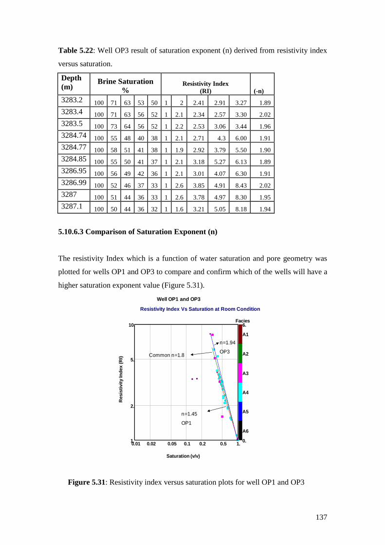
137

Table 5.22: Well OP3 result of saturation exponent (n) derived from resistivity index

versus saturation.

Depth

(m) Brine Saturation

% Resistivity Index

(RI) (-n)

3283.2 100 71 63 53 50 1 2 2.41 2.91 3.27 1.89

3283.4 100 71 63 56 52 1 2.1 2.34 2.57 3.30 2.02

3283.5 100 73 64 56 52 1 2.2 2.53 3.06 3.44 1.96

3284.74 100 55 48 40 38 1 2.1 2.71 4.3 6.00 1.91

3284.77 100 58 51 41 38 1 1.9 2.92 3.79 5.50 1.90

3284.85 100 55 50 41 37 1 2.1 3.18 5.27 6.13 1.89

3286.95 100 56 49 42 36 1 2.1 3.01 4.07 6.30 1.91

3286.99 100 52 46 37 33 1 2.6 3.85 4.91 8.43 2.02

3287 100 51 44 36 33 1 2.6 3.78 4.97 8.30 1.95

3287.1 100 50 44 36 32 1 1.6 3.21 5.05 8.18 1.94

5.10.6.3 Comparison of Saturation Exponent (n)

The resistivity Index which is a function of water saturation and pore geometry was

plotted for wells OP1 and OP3 to compare and confirm which of the wells will have a

higher saturation exponent value (Figure 5.31).

n=1.45

n=1.94

Well OP1 and OP3

Resistivity Index Vs Saturation at Room Condition

0.01 0.02 0.05 0.1 0.2 0.5 1.

Saturation (v/v)

1.

2.

5.

10.

Resis

tivit

y In

dex (

RI)

A6

A5

A4

A3

A2

A1

0.

6.Facies

n=1.94

OP3

n=1.45

OP1

Common n=1.8

Figure 5.31: Resistivity index versus saturation plots for well OP1 and OP3

138

Well OP3 present a cleaner sandstone trend with higher saturation exponent value of

1.94 than OP1 which display a lower saturation exponent mean value of 1.45 as

shown in Figure 5.31. The differences in the saturation exponent trend may be due to

the distribution of fluids within the pore systems and types of facies present. A

common value of saturation index of 1.8 was obtained for both well.

In rocks containing clay minerals such as chlorite, the saturation exponent becomes

increasingly lower as the water saturation is reduced. In most shaly-sand saturation

equations such as the Waxman-Smith and Dual-water models, the value of the

saturation exponent is determined in high water salinity or with the clay effects

removed and the variations of resistivity index with the saturation is then predicted

from equations.

5.10.7 Petrography Studies

The petrography study is defined as the scientific description and study of rocks.

Varieties of techniques and instrumentation have been devised to assist the geologist.

This study includes thin sections, X-Ray Diffraction (XRD), and Scanning Electron

Microscopy (SEM) (Core laboratories, 1982). OMNI laboratories performed the

petrography studies in well OP2 and OP3 within the Albian age formation of the

study area.

The petrography studies is included in this research because it will aid in the mineral

identification and also help in understanding the textural nature of mineral and better

understanding of the pore space as it will be used to validate other results.

5.10.7.1 Thin Section Analysis

Selected reservoir sandstone samples from well OP2 and OP3 were investigated in

thin sections in order to obtain information on the occurrence and distribution of

different mineral components. The information obtained from the thin section

investigations will be used to supplement the quantitative mineralogy data determined

by X-Ray Diffraction and Scanning electron microscopy. The petrophysical properties

of the reservoir sequence studied are influenced not by the proportion of the mineral

constituents alone but also by the way the minerals occur in the rocks.

139

The sandstone samples in thin sections typically consist of quartz as the dominant

framework grains, with minor feldspar and opaque grains. Lithic fragments include

shale, siltstone and quarts. Traces of glauconite, siderite may also be noted in some of

the samples.

5.10.7.1.1 Well OP3

Thin sections of well OP3 are shown in Figure 5.32 below.

Figure 5.32: Well OP3 thin section at depth 3236m and 3283m showing fine grain,

sub angular to angular, and sparely distributed organic matter and pore filling

Chlorite.

Quartz

Pore filling

Chlorite

Organic

Matter

Depth 3236m=Facies A3

20 * µm.

Depth 3236=Facies A3

2 * µm.

Well OP3 Thin Section Photos

Quartz

Pore

Filling

chlorite

Depth 3283m = Facies A3Depth 3283m = facies A3

Well OP3 Thin Section Photos at depth 3283m.

140

They are mostly fine grain, sub-angular to angular and organic matters are sparingly

distributed. The porosities are generally good and grain is dissolved and secondary

porosity observed within the samples (depth 3236m). Fe coatings and little quartz

overgrowth were also observed. The thin sections at depth 3283m look much finer

grains and the organic materials are more as compared to depth 3236m. Pore filling

chlorite clay minerals was also observed. The thin section analysis was performed on

facies A3 in both core of well OP3.

5.10.7.2 X-Ray Diffraction (XRD)

The X-Ray diffraction tests are made on crushed core samples and complement thin

section analysis by providing quantitative mineral identification as Well amount of

clay minerals present in each sample.

Clay minerals comprise of small percentages of the reservoir rock total composition

and it is necessary to separate clay size particles from larger sand grain particles and

make a separate analysis of clay sizes alone. The X-Ray diffraction analysis is more

suitable because it gives more detailed information on different types of clay based on

their unique x-ray diffraction pattern that is comparable to finger print. Samples of

five to ten gram sizes are usually preferred for this analysis. The X- ray diffraction

does not allow identification of non-crystalline (amorphous) materials such as organic

material and volcanic glass.

This analysis was carried out within the Albian age formation of the study area of well

OP2 and OP3 by OMNI laboratories.

5.10.7.2.1 Well OP2 XRD

The whole rock mineralogy results of well OP2 from forest report 2001 is presented

in Table 5.23 below. A total of thirty five samples were taken for analysis and result

shows dominance of quartz having percentage by weight of 67 %, clay minerals with

14 %, and minor occurrences of carbonates and heavy minerals as shown.

141

Table 5.23: Whole rock mineralogy of Well OP2

The X-ray diffraction analysis of the samples indicates the presence of clay mineral as

the dominant clay type in the well. The presence of chlorite and Illite in the samples

will contribute to grain coating. Kaolinite is absent (Figure 5.33) below.

Whole Rock Mineralogy Relative Clay Abundance

(Weight %) (Normalized to 100%)

Depth(m) Quartz Ksp Plag Cal Dol/Fe-Dol Sid Pyr Anh Clay I/S* Ill Chl

3446.00A 75 4 14 0 1 Tr 0 0 6 0 28 72

3446.00B 54 3 12 0 0 1 11 0 19 0 30 70

3447.08 73 2 15 Tr Tr 0 0 0 10 0 24 76

3447.83 62 3 16 0 1 0 1 0 17 0 21 79

3448.69 70 2 17 0 0 Tr 0 0 11 0 25 75

3449.52 70 2 16 0 0 1 Tr 0 11 0 26 74

3450.58 73 2 14 0 Tr 0 0 0 11 0 24 76

3451.70 75 2 13 0 0 Tr 0 0 10 0 21 79

3452.14 77 2 11 0 1 Tr Tr 0 9 0 24 76

3452.59 74 2 12 0 1 0 0 0 11 0 18 82

3453.68 76 2 11 0 0 Tr Tr 0 11 0 26 74

3454.72 78 2 10 0 1 1 Tr 0 8 0 23 77

3455.08 78 2 9 0 2 0 0 0 9 0 24 76

3455.55 69 3 14 0 0 0 Tr 0 14 0 17 83

3455.86 84 2 8 Tr 0 0 Tr 0 6 0 26 74

3456.15 55 3 10 0 0 Tr 0 0 32 0 32 68

3456.65 52 1 9 30 0 Tr 0 0 8 0 31 69

3457.18 37 1 5 31 0 18 0 0 8 0 26 74

3457.74 74 3 12 0 0 0 0 0 11 0 23 77

3458.69 73 2 12 0 1 0 0 0 12 0 20 80

3459.59 75 3 11 0 Tr 1 0 0 10 0 24 76

3460.10 74 3 10 0 2 1 0 1 9 0 24 76

3461.48 75 1 11 0 2 0 0 0 11 0 23 77

3462.54 71 1 14 0 0 1 Tr 0 13 0 22 78

3463.48 73 2 11 0 0 0 0 0 14 0 19 81

3464.59 72 2 11 0 0 0 0 0 15 0 14 86

3464.81 76 1 6 10 0 0 0 0 7 0 23 77

3466.20 72 4 11 1 3 Tr 0 0 9 0 32 68

3466.47 70 2 12 1 0 0 0 0 15 0 18 82

3466.75 49 3 22 0 0 0 1 0 25 0 21 79

3467.50 49 4 10 0 0 0 3 0 34 22 23 55

3468.17 57 2 14 15 0 0 0 0 12 17 25 58

3468.89 65 2 17 3 0 0 1 0 12 13 20 67

3469.39 46 3 19 0 0 0 0 0 32 11 20 69

3470.35 37 3 7 0 0 2 3 0 48 22 34 44

Average: 67 2 12 13 2 3 3 1 14 2 24 74

142

Figure 5.33: Whole rock mineralogy of Well OP2

5.10.7.2.2 Well OP3 XRD

The mineralogy results of fourteen samples within the Albian age from core1 and two

of well OP3 are presented in Table 5.24 below. The results shows the dominance of

quartz percentage by weight of 57 to 58 % in both cores, clay minerals with about 25

and 20 % in both cores, carbonates in small proportions in both cores.

Well OP2 Framework Results

0%

10%

20%

30%

40%

50%

60%

70%

80%

90%

100%

3449.34 3455.48 3459.99 3466.82 3472.23

Depth (m)

Perc

en

tag

e

ClayOthersPlagKspQtz

Well OP2 XRD Clay Type

0%

10%

20%

30%

40%

50%

60%

70%

80%

90%

100%

3449.34 3455.48 3459.99 3466.82 3472.23

Depth (m)

Perc

en

tag

es

Chlorite

Illite

Mixed

Well OP2 XRD Piechart

Chlorite

74%

Illite

24%

Mixed

2%

Chlorite Illite Mixed

Frame work Piechart

Quartz

67%

Clay

14%

Plagioclase

12%

others

5%

K-Feldspar

2%

Quartz Clay Plagioclase others K-Feldspar

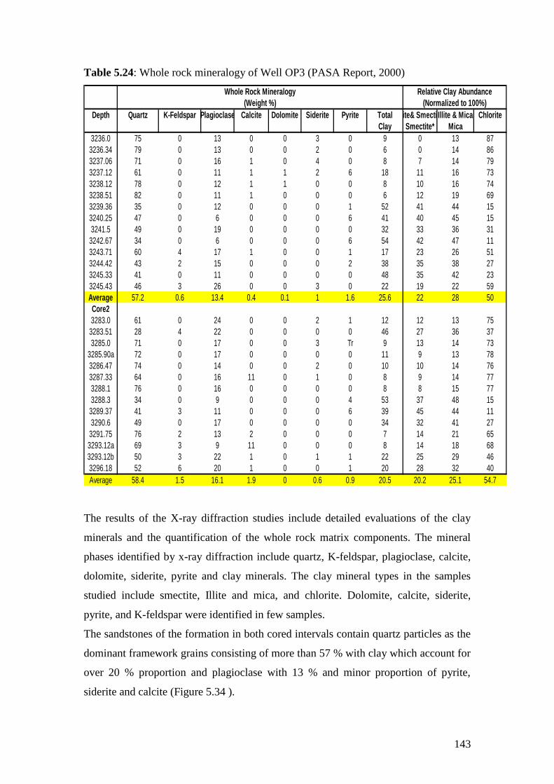
143

Table 5.24: Whole rock mineralogy of Well OP3 (PASA Report, 2000)

Whole Rock Mineralogy Relative Clay Abundance

(Weight %) (Normalized to 100%)

Depth Quartz K-Feldspar Plagioclase Calcite Dolomite Siderite Pyrite Total Illite& SmectiteIllite & Mica Chlorite

Clay Smectite* Mica

3236.0 75 0 13 0 0 3 0 9 0 13 87

3236.34 79 0 13 0 0 2 0 6 0 14 86

3237.06 71 0 16 1 0 4 0 8 7 14 79

3237.12 61 0 11 1 1 2 6 18 11 16 73

3238.12 78 0 12 1 1 0 0 8 10 16 74

3238.51 82 0 11 1 0 0 0 6 12 19 69

3239.36 35 0 12 0 0 0 1 52 41 44 15

3240.25 47 0 6 0 0 0 6 41 40 45 15

3241.5 49 0 19 0 0 0 0 32 33 36 31

3242.67 34 0 6 0 0 0 6 54 42 47 11

3243.71 60 4 17 1 0 0 1 17 23 26 51

3244.42 43 2 15 0 0 0 2 38 35 38 27

3245.33 41 0 11 0 0 0 0 48 35 42 23

3245.43 46 3 26 0 0 3 0 22 19 22 59

Average 57.2 0.6 13.4 0.4 0.1 1 1.6 25.6 22 28 50

Core2

3283.0 61 0 24 0 0 2 1 12 12 13 75

3283.51 28 4 22 0 0 0 0 46 27 36 37

3285.0 71 0 17 0 0 3 Tr 9 13 14 73

3285.90a 72 0 17 0 0 0 0 11 9 13 78

3286.47 74 0 14 0 0 2 0 10 10 14 76

3287.33 64 0 16 11 0 1 0 8 9 14 77

3288.1 76 0 16 0 0 0 0 8 8 15 77

3288.3 34 0 9 0 0 0 4 53 37 48 15

3289.37 41 3 11 0 0 0 6 39 45 44 11

3290.6 49 0 17 0 0 0 0 34 32 41 27

3291.75 76 2 13 2 0 0 0 7 14 21 65

3293.12a 69 3 9 11 0 0 0 8 14 18 68

3293.12b 50 3 22 1 0 1 1 22 25 29 46

3296.18 52 6 20 1 0 0 1 20 28 32 40

Average 58.4 1.5 16.1 1.9 0 0.6 0.9 20.5 20.2 25.1 54.7

The results of the X-ray diffraction studies include detailed evaluations of the clay

minerals and the quantification of the whole rock matrix components. The mineral

phases identified by x-ray diffraction include quartz, K-feldspar, plagioclase, calcite,

dolomite, siderite, pyrite and clay minerals. The clay mineral types in the samples

studied include smectite, Illite and mica, and chlorite. Dolomite, calcite, siderite,

pyrite, and K-feldspar were identified in few samples.

The sandstones of the formation in both cored intervals contain quartz particles as the

dominant framework grains consisting of more than 57 % with clay which account for

over 20 % proportion and plagioclase with 13 % and minor proportion of pyrite,

siderite and calcite (Figure 5.34 ).

144

Figure 5.34: Whole rock mineralogy of core 1 and 2 of well OP3

Whole rock X-Ray Diffraction indicates that Chlorite is the main clay mineral type in

both cored intervals .The proportion of Illitic clay (illite, mixed layer illite-smectite

and mica) was also found with good proportion.

WellOP3 Core 1 XRD Framework

0%

10%

20%

30%

40%

50%

60%

70%

80%

90%

100%

3236.21 3236.55 3237.27 3237.33 3238.33 3238.72 3239.57 3240.46 3241.36 3242.88

Depth (m)

Others

Clay

Plagio

Quartz

welll OP3 core 2 XRD Framework

0%

10%

20%

30%

40%

50%

60%

70%

80%

90%

100%

3283 3283.5 3285 3285.9 3286.5 3287.3 3288.1 3288.3 3289.4 3290.6 3291.8 3293.1

Depth (m)

Others

Clay

Plagio

Kspar

Quartz

Well OP3 Core1 XRD Clay Type

0%

10%

20%

30%

40%

50%

60%

70%

80%

90%

100%

3236.21 3236.55 3237.27 3237.33 3238.33 3238.72 3239.57 3240.46 3241.36 3242.88

Depth (m)

Mixed

Illite

Chlorite

Well OP3 Core 2 XRD Clay Type

0%

10%

20%

30%

40%

50%

60%

70%

80%

90%

100%

3283 3283.5 3285 3285.9 3286.5 3287.3 3288.1 3288.3 3289.4 3290.6 3291.8 3293.1

Depth (m)

Mixed

Illite

Chlorite

145

5.10.7.3 Scanning Electron Microscopy (SEM)

The shale materials in sandstone reservoirs can be distributed in the formation in three

ways which are laminated, structural and dispersed. Shale can exist in the form of a

lamina between layers of clean sand, and could also exist as structural grains or

nodules within the formation matrix. The shaly material could also exist as dispersed

throughout the sand, partially filling the inter-granular interstices or can be coating the

grains (Schlumberger, 1987). Figure 5.35 below presents the three forms of existence

of shale in sandstone reservoirs.

Figure 5.35: Different ways of shale distribution in a formation (Serra, 1984).

The most commonly found clay minerals in sedimentary rocks are the chlorite,

Kaolinite, illite and smectite. The Scanning electron microscopy (SEM) shows images

of these minerals because each has its own unique feature.

The two principle methods used to obtain images applied to reservoir rock samples

are the transmission electron microscopy (TEM) and Scanning electron microscopy

(SEM). In transmission electron microscopy, a high energy beam penetrates an ultra-

thin sample and the image is formed from the projection of the transmitted electrons.

Scanning electron microscopy uses a beam of medium energy electrons to scan the

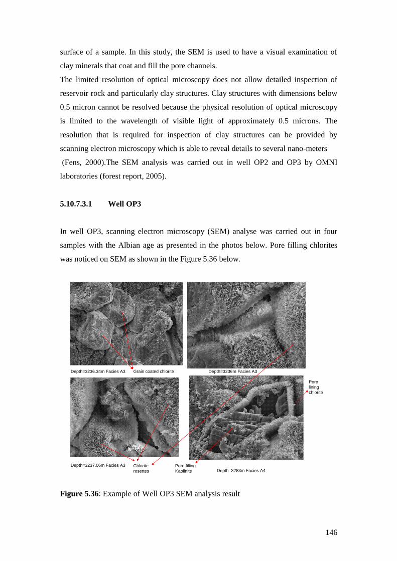
146

surface of a sample. In this study, the SEM is used to have a visual examination of

clay minerals that coat and fill the pore channels.

The limited resolution of optical microscopy does not allow detailed inspection of

reservoir rock and particularly clay structures. Clay structures with dimensions below

0.5 micron cannot be resolved because the physical resolution of optical microscopy

is limited to the wavelength of visible light of approximately 0.5 microns. The

resolution that is required for inspection of clay structures can be provided by

scanning electron microscopy which is able to reveal details to several nano-meters

(Fens, 2000).The SEM analysis was carried out in well OP2 and OP3 by OMNI

laboratories (forest report, 2005).

5.10.7.3.1 Well OP3

In well OP3, scanning electron microscopy (SEM) analyse was carried out in four

samples with the Albian age as presented in the photos below. Pore filling chlorites

was noticed on SEM as shown in the Figure 5.36 below.

Figure 5.36: Example of Well OP3 SEM analysis result

Pore filling

Kaolinite

Pore

lining

chlorite

Depth=3283m Facies A4

Depth=3237.06m Facies A3 Chlorite

rosettes

Depth=3236.34m Facies A3 Depth=3236m Facies A3Grain coated chlorite

147

5.10.7.4 Relationship between Chlorite and Facies

The petrographic analysis analyses revealed mineralogy with quartz being the

dominant mineral in addition to abundant chlorite as the major clay mineral. The fine

textured dispersed pore lining and pore filling chlorite mineral is detrimental to

permeability and hence affect the reservoir quality and may be the possible causes of

the low resistivity, hence the special focus on the effect of chlorite on the facies and

its distribution.

The distribution of chlorite for well OP2 is presented in Figure 5.37 below.

Well OP2

Chlorite Vs Depth and facies

0. 0.06 0.12 0.18 0.24 0.3

Chlorite (v/v)

3475.

3468.8

3462.6

3456.4

3450.2

3444.

De

pth

(m

)

A6

A5

A4

A3

A2

A1

0.

6.

Facies

A6

A2

A1

A2

A3

A4

A5

OP2Scale : 1 : 250


Depth

DEPTH

(M)

GammaRay

GRn (GAPI)0. 200.

Core Facies


Porosity

PhiDen (dec)0.5 0.



AT10 (OHMM)0.2 2000.

AT90 (OHMM)0.2 2000.

Cor Kli (mD)0.001 10000.

3450 Facies A1

Facies A2

Facies A3

Facies A4

Facies A3

Facies A5

Facies A4

Facies A2

Facies A6

3460

3470

Massive

sands

Shale/silt

Sands

Shale

Figure 5.37: Distribution of chlorite for Well OP2

148

The plot shows that facies A1 has the lowest volume of chlorite of less than 3% and

highest amount of chlorite was observed in facies A6 with chlorite volume that range

from 5 % to 20 %. At the shale/silt interval (facies A5 and A6) relatively high chlorite

content was also observed. It can be concluded that in well OP2, textural parameters

and grain composition has a relationship with chlorite mineral in the pore-space of

sandstone reservoirs.

The chlorite distribution with facies for well OP3 core 1 is presented in Figure 5.38 a

below.

Figure 5.38a: Well OP3 core 1 chlorite distribution

In core 1 of well OP3, the highest amount of chlorite was observed in facies A3 in the

range of 9 % to 11 %. The least amount of chlorite was recorded in facies A4.

However, within the reservoir area (3235m to 3240m) the amount of chlorite tends to

OP3Scale : 1 : 200


1

DEPTH

(M)

Gamma Ray

GrC (GAPI)0. 150.

LithoFacies


Porosity


Cor Poro ()0.5 0.


ILD (OHMM)0.2 2000.


Cor Klin ()0.001 1000.

3225

Facies A3

Facies A4

Facies A5

Facies A6

3230

3235

Well OP3 ( Core 1)

Chlorite Vs Depth and Facies Plot

0. 4. 8. 12. 16. 20.

Chlorite (%)

3250

3245

3240

3235

3230

3225.

dep

th (

m)

A6

A5

A4

A3

A2

A1

0.

6.

Facies

A6

A5

A4

A3

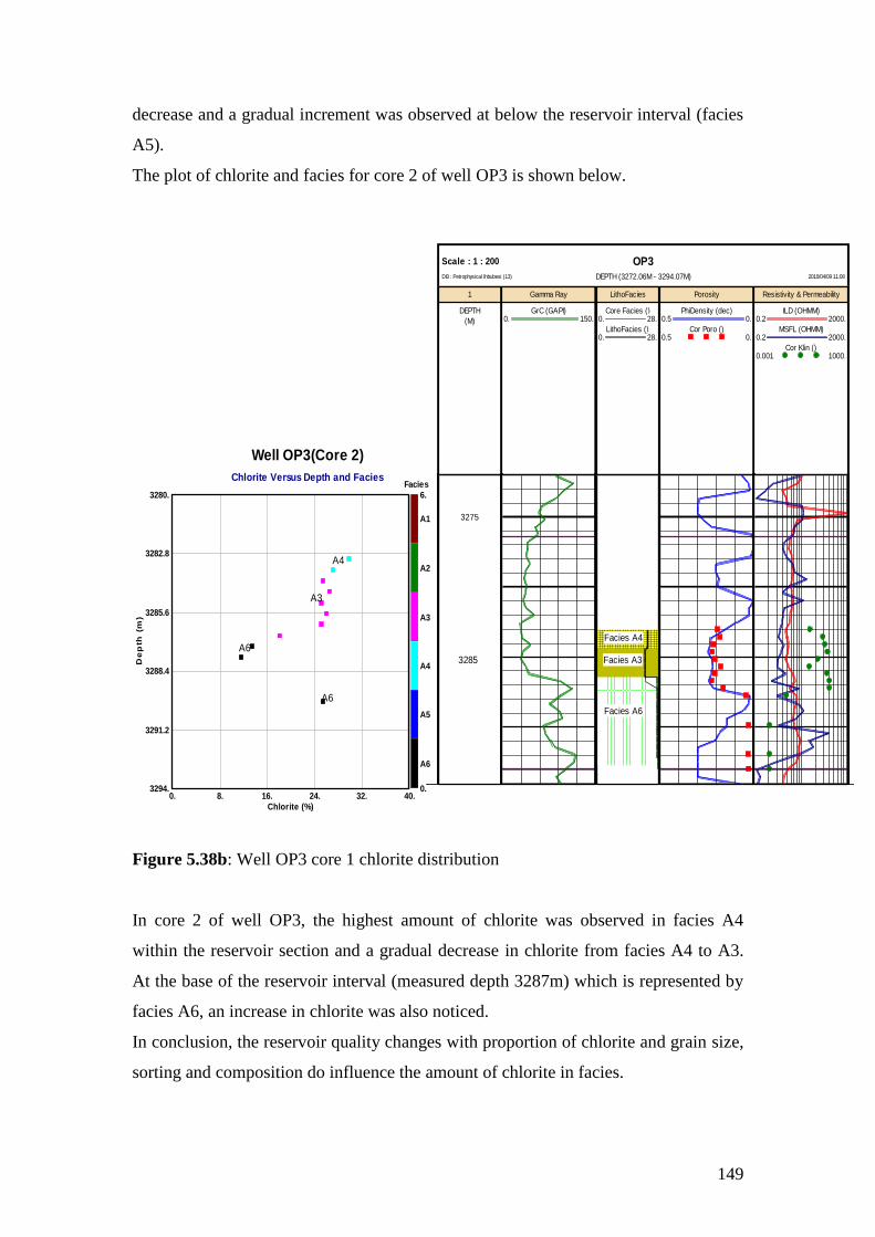
149

decrease and a gradual increment was observed at below the reservoir interval (facies

A5).

The plot of chlorite and facies for core 2 of well OP3 is shown below.

OP3Scale : 1 : 200


1

DEPTH

(M)

Gamma Ray

GrC (GAPI)0. 150.

LithoFacies



Porosity


Cor Poro ()0.5 0.


ILD (OHMM)0.2 2000.


Cor Klin ()0.001 1000.

3275

Facies A3

Facies A4

Facies A5

Facies A6

Facies A4

Facies A3

Facies A6

3285

Well OP3(Core 2)

Chlorite Versus Depth and Facies

0. 8. 16. 24. 32. 40.

Chlorite (%)

3294.

3291.2

3288.4

3285.6

3282.8

3280.

De

pth

(m

)

A6

A5

A4

A3

A2

A1

0.

6.

Facies

A6

A6

A3

A4

Figure 5.38b: Well OP3 core 1 chlorite distribution

In core 2 of well OP3, the highest amount of chlorite was observed in facies A4

within the reservoir section and a gradual decrease in chlorite from facies A4 to A3.

At the base of the reservoir interval (measured depth 3287m) which is represented by

facies A6, an increase in chlorite was also noticed.

In conclusion, the reservoir quality changes with proportion of chlorite and grain size,

sorting and composition do influence the amount of chlorite in facies.

150

5.10.8 Cation Exchange Capacity (CEC)

The cation exchange capacity (CEC) is an important property of clay in shaly sand

evaluation because it is the source of the excess conductivity in addition to the

formation salinity. The cation exchange capacity (CEC) actually measures the

concentration of sodium cations by chemical means and is termed cation exchange

capacity and it is a reflection of the specific surface area of clay regardless of type.

The results from this measurement can be related to the clay bound water and also

help to identify producible shaly sands.

Crystalline surfaces of clay have what is known as exchange sites where ions can

temporarily reside because of the charge imbalance on the external surface of clay‟s

molecular building blocks (Bate, 1985).These exchange sites offer an electrical path

through the clay by means of surface conductance. When in contact with saline

solution, the cations on the surface layers of clay may be easily exchanged by other

cations and are called exchangeable cations. The number of these cations can be

measured and is called cation exchange capacity. The higher the amount of these

cations in the formation, the higher the cation exchange capacity in the formation

which implies higher surface conductance of clays. This shows that CEC can be used

as an effective shaliness indicator.

The cation exchange capacity models result from a phenomena called the double

layer. Winsaur and Mc Cardell (1953) are the first that introduced the double layer

model. They stated that the excess conductivity, the double layer conductivity of shaly

reservoir rocks was attributed to absorption on the clay surface and a resultant

concentration of ions adjacent to this surface (Worthington, 1985).The most

commonly used CEC models are the Waxman-Smith and Dual-Water shaly sand

models.

Cation exchange capacity is expressed in milli-equivalents per gram of dry clay. For

practical purpose Qv, the cation exchange capacity per unit pore volume is used. For

petrophysical evaluations, the cation exchange capacity is commonly determined by

using the titration method using barium chlorite at or ammonium acetate. A piece of

core plug end was crushed and weighed and a solution was used to exchange the

cations. The solution was titrated while the conductivity also was monitored and CEC

measured. For this study, the core plug samples were crushed and weighed and then

sent to the Agricultural Research Council (ARC) Pretoria South Africa were the

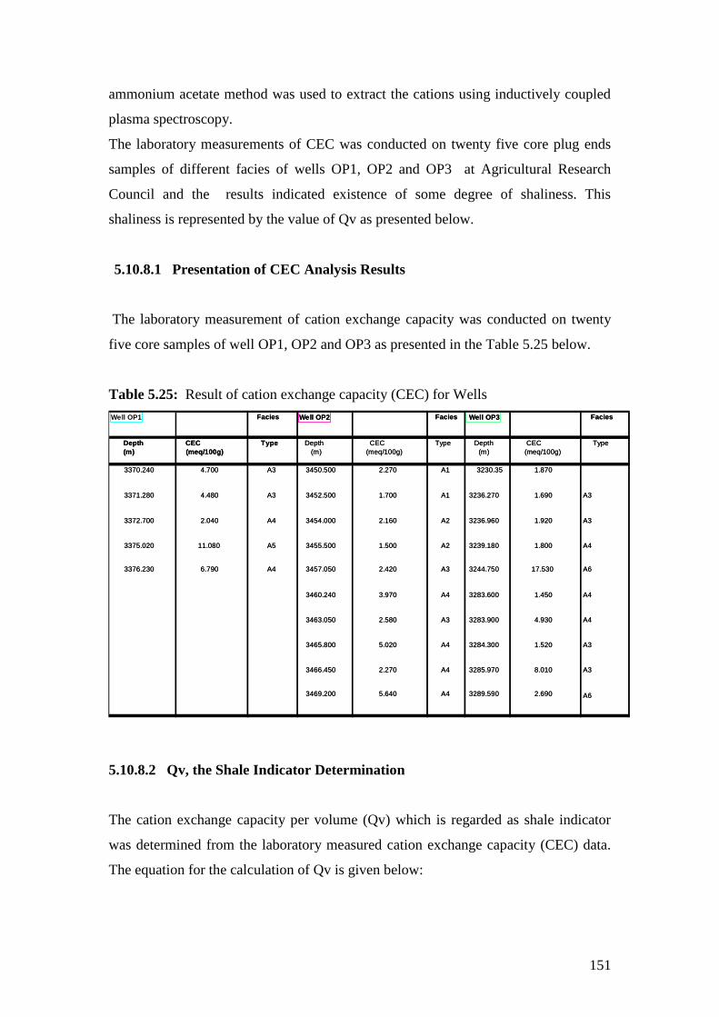
151

ammonium acetate method was used to extract the cations using inductively coupled

plasma spectroscopy.

The laboratory measurements of CEC was conducted on twenty five core plug ends

samples of different facies of wells OP1, OP2 and OP3 at Agricultural Research

Council and the results indicated existence of some degree of shaliness. This

shaliness is represented by the value of Qv as presented below.

5.10.8.1 Presentation of CEC Analysis Results

The laboratory measurement of cation exchange capacity was conducted on twenty

five core samples of well OP1, OP2 and OP3 as presented in the Table 5.25 below.

Table 5.25: Result of cation exchange capacity (CEC) for Wells

5.10.8.2 Qv, the Shale Indicator Determination

The cation exchange capacity per volume (Qv) which is regarded as shale indicator

was determined from the laboratory measured cation exchange capacity (CEC) data.

The equation for the calculation of Qv is given below:

Well OP1 Facies Well OP2 Facies Well OP3 Facies

Depth

(m)

CEC

(meq/100g)

Type Depth

(m)

CEC

(meq/100g)

Type Depth

(m)

CEC

(meq/100g)

Type

3370.240 4.700 A3 3450.500 2.270 A1 3230.35 1.870

3371.280 4.480 A3 3452.500 1.700 A1 3236.270 1.690 A3

3372.700 2.040 A4 3454.000 2.160 A2 3236.960 1.920 A3

3375.020 11.080 A5 3455.500 1.500 A2 3239.180 1.800 A4

3376.230 6.790 A4 3457.050 2.420 A3 3244.750 17.530 A6

3460.240 3.970 A4 3283.600 1.450 A4

3463.050 2.580 A3 3283.900 4.930 A4

3465.800 5.020 A4 3284.300 1.520 A3

3466.450 2.270 A4 3285.970 8.010 A3

3469.200 5.640 A4 3289.590 2.690 A6

Well OP1 Facies Well OP2 Facies Well OP3 Facies

Depth

(m)

CEC

(meq/100g)

Type Depth

(m)

CEC

(meq/100g)

Type Depth

(m)

CEC

(meq/100g)

Type

3370.240 4.700 A3 3450.500 2.270 A1 3230.35 1.870

3371.280 4.480 A3 3452.500 1.700 A1 3236.270 1.690 A3

3372.700 2.040 A4 3454.000 2.160 A2 3236.960 1.920 A3

3375.020 11.080 A5 3455.500 1.500 A2 3239.180 1.800 A4

3376.230 6.790 A4 3457.050 2.420 A3 3244.750 17.530 A6

3460.240 3.970 A4 3283.600 1.450 A4

3463.050 2.580 A3 3283.900 4.930 A4

3465.800 5.020 A4 3284.300 1.520 A3

3466.450 2.270 A4 3285.970 8.010 A3

3469.200 5.640 A4 3289.590 2.690 A6

152

Qv = CEC (1 – Φ ) ρma..............................................(5.11)

Φ * 100

Where:

Qv = Cation exchange capacity per pore volume

CEC = cation exchange capacity

ρma=Grain density (g/cc)

Φ = Porosity (fraction)

Applying equation 5.11, the following values for Qv were obtained:

Table 5.26: Calculated values of cation exchange capacity per pore volume for Wells

Well OP1

Well OP2

Well OP3

Depth

(m) CEC

(meq/100g) Qv

(meq/l) Depth (m)

CEC

(meq/100g) Qv

(meq/l) Depth (m)

CEC

(meq/100g) Qv

(meq/l) 3370.240 4.700 0.532428 3450.500 2.270 0.212762 3230.35 1.870 Nil

3371.280 4.480 0.618885 3452.500 1.700 0.144273 3236.270 1.690 0.15511508

3372.700 2.040 0.588528 3454.000 2.160 0.193799 3236.960 1.920 0.19110819

3375.020 11.080 9.637015 3455.500 1.500 0.174926 3239.180 1.800 1.07362047

3376.230 6.790 2.165022 3457.050 2.420 1.964299 3244.750 17.530 7.332799

3460.240 3.970 0.355514 3283.600 1.450 0.17945461

3463.050 2.580 0.285748 3283.900 4.930 0.61014566

3465.800 5.020 4.463617 3284.300 1.520 0.15051283

3466.450 2.270 0.930693 3285.970 8.010 1.02235843

3469.200 5.640 1.96272 3289.590 2.690 3.07376943

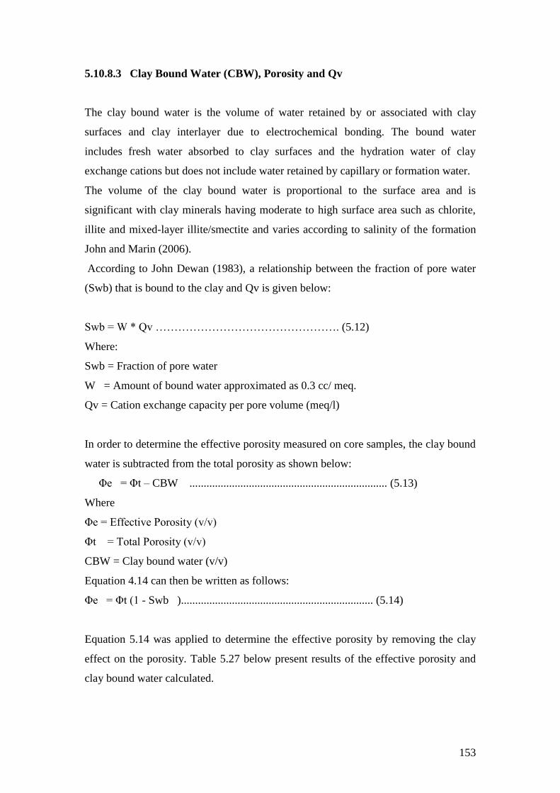
153

5.10.8.3 Clay Bound Water (CBW), Porosity and Qv

The clay bound water is the volume of water retained by or associated with clay

surfaces and clay interlayer due to electrochemical bonding. The bound water

includes fresh water absorbed to clay surfaces and the hydration water of clay

exchange cations but does not include water retained by capillary or formation water.

The volume of the clay bound water is proportional to the surface area and is

significant with clay minerals having moderate to high surface area such as chlorite,

illite and mixed-layer illite/smectite and varies according to salinity of the formation

John and Marin (2006).

According to John Dewan (1983), a relationship between the fraction of pore water

(Swb) that is bound to the clay and Qv is given below:

Swb = W * Qv …………………………………………. (5.12)

Where:

Swb = Fraction of pore water

W = Amount of bound water approximated as 0.3 cc/ meq.

Qv = Cation exchange capacity per pore volume (meq/l)

In order to determine the effective porosity measured on core samples, the clay bound

water is subtracted from the total porosity as shown below:

Φe = Φt – CBW ...................................................................... (5.13)

Where

Φe = Effective Porosity (v/v)

Φt = Total Porosity (v/v)

CBW = Clay bound water (v/v)

Equation 4.14 can then be written as follows:

Φe = Φt (1 - Swb ).................................................................... (5.14)

Equation 5.14 was applied to determine the effective porosity by removing the clay

effect on the porosity. Table 5.27 below present results of the effective porosity and

clay bound water calculated.

154

Table 5.27: Calculated effective porosity and clay bound water for Wells

Three of the core sample plugs one each from each well was not used for other

analysis because they gave erroneous values. The Qv was plotted against the

fractional values of pore water saturation (Swb) on a linear scale for all the wells in

Figure 5.39 below.

Well OP1

Depth (m) CEC(meq/100g) Qv (meq/l) Swb (v/v) Φt (v/v) Φe (v/v) CBW (v/v) Remark

3370.240 4.700 0.5324279 0.159 0.189 0.158 0.031

3371.280 4.480 0.6188847 0.186 0.164 0.133 0.031

3372.700 2.040 0.588528 0.177 0.085 0.069 0.016

3375.020 11.080 9.6370147 2.89 0.03 -0.056 Not Used3376.230 6.790 2.1650224 0.65 0.077 0.027 0.05

Well OP2 CEC(meq/100g) Swb

(v/v)

Φt (v/v) Φe (v/v) CBW (v/v)

Depth (m)

3450.500 2.270 0.2127621 0.063 0.223 0.208 0.015

3452.500 1.700 0.1442733 0.04 0.24 0.229 0.011

3454.000 2.160 0.193799 0.058 0.23 0.216 0.014

3455.500 1.500 0.1749255 0.052 0.188 0.178 0.013457.050 2.420 1.9642993 0.58 0.033 0.0135 0.0195

3460.240 3.970 0.3555144 0.11 0.231 0.206 0.025

3463.050 2.580 0.2857482 0.85 0.196 0.179 0.017

3465.800 5.020 4.4636167 1.33 0.03 -0.01 0.04 Not Used

3466.450 2.270 0.9306927 0.27 0.062 0.044 0.0183469.200 5.640 1.96272 0.588 0.072 0.029 0.043


(v/v)

Φt

(v/v)

Φe

(v/v)

CBW

(v/v)Depth (m)

3230.35 1.870

3236.270 1.690 0.1551151 0.046 0.226 0.215 0.011

3236.960 1.920 0.1911082 0.057 0.214 0.2 0.014

3239.180 1.800 1.0736205 0.322 0.043 0.029 0.014

3244.750 17.530 7.332799 2.199 0.06 -0.07 Not Used3283.600 1.450 0.1794546 0.053 0.178 0.1684 0.0096

3283.900 4.930 0.6101457 0.183 0.178 0.1454 0.0326

3284.300 1.520 0.1505128 0.045 0.213 0.2033 0.0097

3285.970 8.010 1.0223584 0.3 0.173 0.119 0.0543289.590 2.690 3.0737694 0.92 0.023 0.0017 0.0213

Well OP1

Depth (m) CEC(meq/100g) Qv (meq/l) Swb (v/v) Φt (v/v) Φe (v/v) CBW (v/v) Remark

3370.240 4.700 0.5324279 0.159 0.189 0.158 0.031

3371.280 4.480 0.6188847 0.186 0.164 0.133 0.031

3372.700 2.040 0.588528 0.177 0.085 0.069 0.016

3375.020 11.080 9.6370147 2.89 0.03 -0.056 Not Used3376.230 6.790 2.1650224 0.65 0.077 0.027 0.05


(v/v)

Φt (v/v) Φe (v/v) CBW (v/v)

Depth (m)

3450.500 2.270 0.2127621 0.063 0.223 0.208 0.015

3452.500 1.700 0.1442733 0.04 0.24 0.229 0.011

3454.000 2.160 0.193799 0.058 0.23 0.216 0.014

3455.500 1.500 0.1749255 0.052 0.188 0.178 0.013457.050 2.420 1.9642993 0.58 0.033 0.0135 0.0195

3460.240 3.970 0.3555144 0.11 0.231 0.206 0.025

3463.050 2.580 0.2857482 0.85 0.196 0.179 0.017

3465.800 5.020 4.4636167 1.33 0.03 -0.01 0.04 Not Used

3466.450 2.270 0.9306927 0.27 0.062 0.044 0.0183469.200 5.640 1.96272 0.588 0.072 0.029 0.043


(v/v)

Φt

(v/v)

Φe

(v/v)

CBW

(v/v)Depth (m)

3230.35 1.870

3236.270 1.690 0.1551151 0.046 0.226 0.215 0.011

3236.960 1.920 0.1911082 0.057 0.214 0.2 0.014

3239.180 1.800 1.0736205 0.322 0.043 0.029 0.014

3244.750 17.530 7.332799 2.199 0.06 -0.07 Not Used3283.600 1.450 0.1794546 0.053 0.178 0.1684 0.0096

3283.900 4.930 0.6101457 0.183 0.178 0.1454 0.0326

3284.300 1.520 0.1505128 0.045 0.213 0.2033 0.0097

3285.970 8.010 1.0223584 0.3 0.173 0.119 0.0543289.590 2.690 3.0737694 0.92 0.023 0.0017 0.0213

Qv (meq/l Remark

Remark

155

Figure 5.39: Plot of Qv versus saturation of bound water for all Well.

It was observed from the plot that core facies A1 and A2 have very low amount of

cation exchange capacity per pore volume (Qv) and saturation of bound water (Swb).

Highest amount of both Qv (2.69 meq/l) and saturation of bound water (92 %) was

observed in facies A6. It could be interpreted that Facies A6 would retain the highest

amount of bound water in its surfaces, followed by Facies A4, A3 and A2 and A1.

Generally, as the amount of cation capacity per pore volume increases, the amount of

clay increases and the saturation of bound water also increases.

A linear empirical relationship was established from the cross plot as follows

Qv = 3.3333 * (Swb) .................................................................................... (5.15)

R2 =0.99864

The cation exchange capacity per pore volume (Qv) was also plotted against

porosity on a linear scale to establish an empirical relationship between them as

shown in Figure 5.40a below.

All Well

Qv Versus Saturation of bound water Plot

0.01 0.208 0.406 0.604 0.802 1.

Saturation of bound water (v/v)

0.

0.8

1.6

2.4

3.2

4.

Cati

on

Exch

an

ge C

ap

acit

y p

er

Po

re V

olu

me (

Qv)

(meq

/l)

A6

A5

A4

A3

A2

A1

0.

6.Facies

Qv = 0.0000 + 3.3333 * Swb

R2= 0.99864 A6

A4

Incr

easin

g am

ount o

f cla

y

Clean

sand

Clay

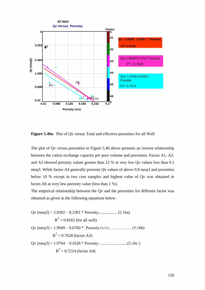
156

Figure 5.40a: Plot of Qv versus Total and effective porosities for all Well

The plot of Qv versus porosities in Figure 5.40 above presents an inverse relationship

between the cation exchange capacity per pore volume and porosities. Facies A1, A2,

and A3 showed porosity values greater than 12 % at very low Qv values less than 0.1

meq/l. While facies A4 generally presents Qv values of above 0.8 meq/l and porosities

below 10 % except in two core samples and highest value of Qv was obtained in

facies A6 at very low porosity value (less than 1 %).

The empirical relationship between the Qv and the porosities for different facies was

obtained as given in the following equations below.

Qv (meq/l) = 2.0302 – 8.2301 * Porosity.................. (5.16a)

R2 = 0.8165 (for all well)

Qv (meq/l) = 1.9949 – 9.0760 * Porosity (v/v)…………….. (5.16b)

R2 = 0.7628 (facies A3)

Qv (meq/l) = 1.9764 – 9.4326 * Porosity ...........................(5.16c )

R2 = 0.7214 (facies A4)

All Well

Qv Versus Porosity

0.01 0.068 0.126 0.184 0.242 0.3

Porosity (v/v)

0.01

0.808

1.606

2.404

3.202

4.Q

v (

meq

/l)

A6

A5

A4

A3

A2

A1

0.

6.Facies

Qv = 2.0302 -8.2301 * Porosity

R2= 0.8165

A4A3

A6

A1A2

Qv=1.9949-9.0760* Porosity

R2 = 0.7628

Qv= 1.9764-9.4326 *

Porosity

R2= 0.7214

157

An empirical relationship between saturation of bound water and porosity was also

determined through the linear cross plot of porosity versus saturation of bound water.

The idea is to be able to predict saturation of bound water from log porosity in Wells

without Qv data. The saturation of bound water is required in calculation of water

saturation using the cation exchange capacity shaly sand model.

The plot is presented in Figure 5.40b below.

Multi-Well Porosity Vs Bound Water

y = -2.7744x + 0.6647

R² = 0.7008

0

0.1

0.2

0.3

0.4

0.5

0.6

0.7

0.8

0.9

1

0 0.05 0.1 0.15 0.2 0.25 0.3

Porosity (v/v)

Satu

rati

on

of

Bo

un

d W

ate

r(v/

v)

Figure 5.40b: Multi-Well porosity versus saturation of bound water plot.

An empirical relationship was established from the cross plot with good regression

coefficient as given in the equation below.

Swb = 0.6647 – 2.7744 * Porosity ………………………………(5.16d)

R2 =0.7008

It could be concluded from the cation exchange capacity analysis that shaly sands

with cation exchange capacity per pore volume (Qv) value higher than 1 have higher

quantity of clay bound water as indicated in the saturation of bound water (Swb)

values. As the Qv increases there is a corresponding increase in saturation of bound

158

water (Figure 5.39 and Table 5.30) meaning that more water will be bound at the

surfaces of the shaly sand formation.

It was also observed that cation exchange capacity has a good relationship with

porosity. At low Qv values, porosities tend to increase as shown in the cross plots of

Figure 5.40. Facies A6 has the highest bound water retention capacity and facies A1

and A 2 the least bound water retention capacity.

5.10.9 Capillary Pressure Measurements

Capillary Pressure is defined as the difference in pressure between the non-wetting

and wetting phases of fluid. The difference in pressure causes the interface between

the two phases to be curved. The curvature of the interface between the two fluids and

the shape of the pore space or the grain determine the saturation of the two phases.

The relationship between the saturation and the capillary pressure is expressed in

terms of a capillary pressure curve. The capillary pressure curves may be determined

under drainage or imbibition conditions. Under drainage condition, a non-wetting

phase is displacing a wetting phase; an example is mercury displacing air. Under

imbibition condition, a wetting phase is displacing a non wetting phase; example is

displacement of oil by water in water wet rock.

The special core analysis capillary pressure measurements are measurements made on

core plugs at increasing pressures. The laboratory capillary pressure curves are used to

define water saturations, pore throat size and distribution, depth of reservoir fluid

contacts, and computation of height above free water level, transition zone height and

relative permeability.

The capillary measurements are of three types. They are the restored porous plates,

centrifuge capillary pressure, and the mercury injection measurements. The results

from the capillary pressure measurements gives location and amount of irreducible

and mobile water saturations, identifies hydraulic units in pressure communication,

highlights rock type differences, height and location of reservoir transition zones, and

pore entry pressure.

The restored state cell (Air-Brine porous plate cell) method involves cleaning and

drying of samples and pressure saturated with simulated formation brine. The fully

saturated samples are placed in a porous plate cell and de-saturated using humidified

nitrogen as the displacing phase at increasing incremental pressures up to 180 psig.

159

After a minimum of four days at each pressure, equilibrium saturations are determined

gravimetrically. These measurements were performed in two wells (OP1 and OP3).

The mercury injection capillary pressure measurements method was made on three

core plugs of well OP2. Before carrying out the measurements, the core plug samples

were cleaned using a simple distillation to extract hydrocarbon and other pore-fillings.

Compound and samples were dried to remove residual moisture. Injected mercury

was monitored at 52 pressure points from 1.01 to 54,900 psia.

The results from this analysis include drainage curves for each sample based on

wetting phase saturation, pore aperture diameter distribution, and mercury derived

porosity and permeability.

5.10.9.1 Well OP1 Air-Brine Capillary Pressure Measurement Results

The restored state cell capillary pressure method was performed on four core plug

samples at increasing pressures from 2 to 180 psig (Table 5.28).

Table 5.28: Well OP1 capillary pressure test data

5.10.9.2 Well OP3 Air-Brine Capillary Pressure Measurement Results

The air-brine restored state cell capillary pressure measurement method was

performed on ten core plug samples of well OP3 as presented in Table 5.29 below.

180803515525764713372.3

180803515844245485156753371.6

180803515844042454851643371

180803515842434650525771913370.4

Capillary Pressure

(psi)

Brine saturation

(%)

Depth

(m)

180803515525764713372.3

180803515844245485156753371.6

180803515844042454851643371

180803515842434650525771913370.4

Capillary Pressure

(psi)

Brine saturation

(%)

Depth

(m)

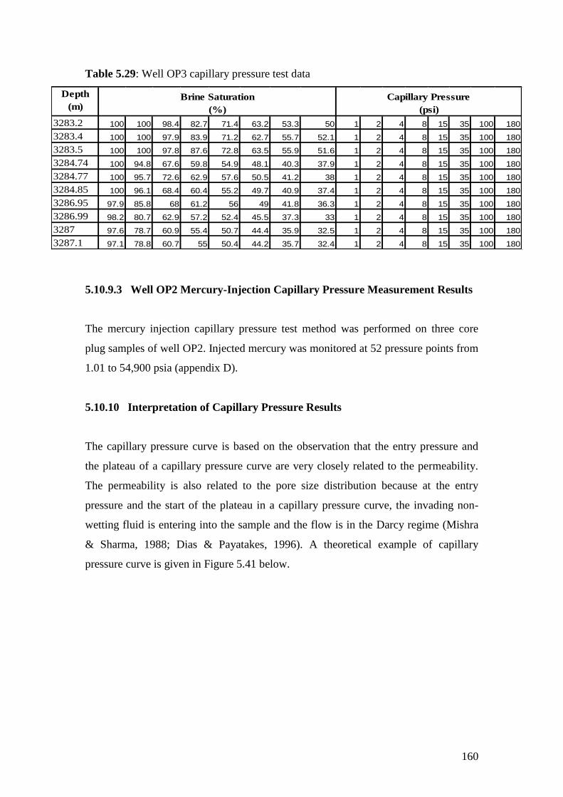
160

Table 5.29: Well OP3 capillary pressure test data

5.10.9.3 Well OP2 Mercury-Injection Capillary Pressure Measurement Results

The mercury injection capillary pressure test method was performed on three core

plug samples of well OP2. Injected mercury was monitored at 52 pressure points from

1.01 to 54,900 psia (appendix D).

5.10.10 Interpretation of Capillary Pressure Results

The capillary pressure curve is based on the observation that the entry pressure and

the plateau of a capillary pressure curve are very closely related to the permeability.

The permeability is also related to the pore size distribution because at the entry

pressure and the start of the plateau in a capillary pressure curve, the invading non-

wetting fluid is entering into the sample and the flow is in the Darcy regime (Mishra

& Sharma, 1988; Dias & Payatakes, 1996). A theoretical example of capillary

pressure curve is given in Figure 5.41 below.

Depth

(m)

3283.2 100 100 98.4 82.7 71.4 63.2 53.3 50 1 2 4 8 15 35 100 180

3283.4 100 100 97.9 83.9 71.2 62.7 55.7 52.1 1 2 4 8 15 35 100 180

3283.5 100 100 97.8 87.6 72.8 63.5 55.9 51.6 1 2 4 8 15 35 100 180

3284.74 100 94.8 67.6 59.8 54.9 48.1 40.3 37.9 1 2 4 8 15 35 100 180

3284.77 100 95.7 72.6 62.9 57.6 50.5 41.2 38 1 2 4 8 15 35 100 180

3284.85 100 96.1 68.4 60.4 55.2 49.7 40.9 37.4 1 2 4 8 15 35 100 180

3286.95 97.9 85.8 68 61.2 56 49 41.8 36.3 1 2 4 8 15 35 100 180

3286.99 98.2 80.7 62.9 57.2 52.4 45.5 37.3 33 1 2 4 8 15 35 100 180

3287 97.6 78.7 60.9 55.4 50.7 44.4 35.9 32.5 1 2 4 8 15 35 100 180

3287.1 97.1 78.8 60.7 55 50.4 44.2 35.7 32.4 1 2 4 8 15 35 100 180

Brine Saturation

(%)

Capillary Pressure

(psi)

161

Figure 5.41: Schematic relationship between capillary pressure curve and oil

accumulation (Holmes, 2002).

The standard techniques to obtain the capillary pressure curves are the porous plate

method, centrifuge and the air-mercury injection methods. Application of the capillary

pressure curve is the estimation of the irreducible water saturation (Swirr) which is

used to determine the maximum volume of hydrocarbons in the reservoir and the

mobile water saturation (Sw).The hydrocarbon-water contact is the maximum depth

with either water free production or economic production. The free water level is

regarded as the intersection of hydrocarbon pressure gradient line and water pressure

gradient line where hydrocarbon and water pressure are equal.

The restored state cell (Air-Brine porous plate cell) method was conducted on

fourteen samples in well OP1 and OP3, while the mercury injection capillary pressure

method was applied on three samples of well OP2.

5.10.10.1 Well OP1 Water Saturation Determination from Capillary Pressure

Curves

The porous plate method of capillary pressure measurement was undertaken on four

samples of well OP1 (Table 5.28) above. To construct the curve, the capillary

162

pressure data measurement at laboratory condition was plotted on the y-axis against

the brine saturation on linear scales as shown (Figure 5.42).

Figure 5.42: Capillary pressure curve for well OP1

The capillary pressure curve of the well indicate the minimum irreducible water

saturation (Swirr) of about 42 % at measured depth 3271m of facies A4 , while the

highest irreducible water saturation of about 56 % was observed of facies A5 at

measured depth of 3372.3m . The differences in the irreducible water saturation may

be attributed to clay type and mode of distribution and pore geometry, permeability

and the type of facies.

The point at which the capillary pressure is zero is equivalent to the free water level.

The transition zone (point were hydrocarbon and water could be produce) would have

been sharp if all the pores are of the same size. At depth 3372.3m (facies type A5),

different pore size is clearly shown (Figure 5.42) and this may be fine grain that has

the ability to retain high amount of irreducible water.

Well OP1

Capillary Pressure Vs Saturation

0. 0.2 0.4 0.6 0.8 1.

Plug Saturation (v/v)

0.

40.

80.

120.

160.

200.

Ca

pil

lary

Pre

ss

ure

(p

si)

A5

Transition

Zone

Oil/Gas

Zone

A4

Facies

Free water

Level

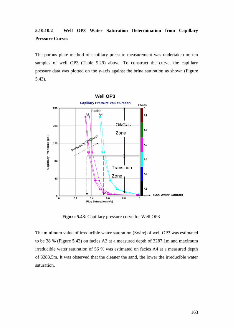
163

5.10.10.2 Well OP3 Water Saturation Determination from Capillary

Pressure Curves

The porous plate method of capillary pressure measurement was undertaken on ten

samples of well OP3 (Table 5.29) above. To construct the curve, the capillary

pressure data was plotted on the y-axis against the brine saturation as shown (Figure

5.43).

Figure 5.43: Capillary pressure curve for Well OP3

The minimum value of irreducible water saturation (Swirr) of well OP3 was estimated

to be 38 % (Figure 5.43) on facies A3 at a measured depth of 3287.1m and maximum

irreducible water saturation of 56 % was estimated on facies A4 at a measured depth

of 3283.5m. It was observed that the cleaner the sand, the lower the irreducible water

saturation.

Well OP3


0. 0.2 0.4 0.6 0.8 1.


0.

40.

80.

120.

160.

200.

Ca

pil

lary

Pre

ss

ure

(p

si)

A6

A5

A4

A3

A2

A1

0.

6.

Facies

A3 A4Facies

Increasing Shaliness

Transition

Zone

Oil/Gas

Zone

Gas Water Contact

164

5.10.10.3 Well OP2 Water Saturation Determination from Capillary

Pressure Curves

The mercury injection capillary pressure method was performed on three core samples

of well OP2. Injected mercury was monitored at 52 pressure points from 1.01 to

54,900 psia (appendix D). Figure 5.44 below present the linear scale plot of injected

mercury pressure against saturation.

Figure 5.44: Capillary Pressure Curve for Well OP2

The minimum point of irreducible water saturation was estimated at about 11 % at a

measured depth of 3447.08m which represents core facies A2, while the highest

irreducible water saturation was observed at depth 3467.5m which represents core

facies A6 with an estimated value of about 84 %. This shows that non reservoir rock

samples like facies A6 gives very high values of irreducible water saturation values

and therefore may not be useful for further analysis.

The point at which the capillary pressure is zero equals to the free water level. The

possible gas water contact (GWC) for this well was located at the free water level.

Well OP2

Capillary Pressure Vs Saturation Plot

0. 0.2 0.4 0.6 0.8 1.


0.

2000.

4000.

6000.

8000.

10000.

Ca

pil

lary

Pre

ss

ure

(p

si)

A6

A5

A4

A3

A2

A1

0.

6.

Facies

A6

A4A2

Increasing Shalin

ess

165

Above the gas water contact, it is expected that oil will displace water first in the large

pores, then in the medium pores, and finally in a smaller pores as elevation increases.

The medium grains will be associated with depth 3447.08m and fine grains at depth

3467.5m.

Comparison of the mercury injection with the porous plate capillary pressure

measurement showed that the mercury injection measurements do not provide a

corresponding measurement for oil and water system but shows how various rock

types can expel a non-wetting phase when pressure is reduced. The porous-plate

capillary pressure method gives accurate results irrespective of the types of facies or

rock measured. Mercury injection also provides the same good results as well but a

scaling factor equal to the interfacial tensions ratio and a contact angle equal to zero is

often used (Omeregie, 1986).

The mercury injection method is a repetitive and fast method but the representative of

the capillary pressures are doubtful for high clay content porous media (Gauchet,

1993).

A plot of capillary pressure curves with porosity and permeability clearly showed that

as the sandstone becomes cleaner and as permeability increases, the irreducible water

saturation becomes smaller (Figure 5.45) below. Porosity does not have much effect

on capillary pressure curves as shown in the Figure 5.45 below.

Well OP1 and OP3

Capillary Pressure Vs Saturation and Permeability Plot

0. 0.2 0.4 0.6 0.8 1.


0.

40.

80.

120.

160.

200.

Ca

pil

lary

Pre

ss

ure

(p

si)

0.

40.

80.

120.

160.

200.

Permeability (mD)

Well OP1 and OP3

Capillary Pressure Vs Saturation and Porosity Plot

0. 0.2 0.4 0.6 0.8 1.


0.

40.

80.

120.

160.

200.

Ca

pil

lary

Pre

ss

ure

(p

si)

0.

0.1

0.2

0.3

Porosity (v/v)

Figure 5.45: Capillary pressure curves with permeability and porosity

In conclusion, it has been demonstrated that coarse-grained sandstones and other

rocks with large pores will have relatively low irreducible water saturation and good

166

to excellent permeability values. Facies A2 present value of irreducible water

saturation of less than 12%; facies A3 in the range of 38 to 44 %; facies A4 between

52 to 56 %; facies A5 about 58 %, and facies A6 of 84 %. Fine-grained sandstones

and rocks with small pores tend to have relatively high irreducible water saturation.

Permeability also depends on pore dimensions and sandstones with large connected

pores have high permeability values while fine-grained sandstones have low

permeability values. Porosity however does not necessarily depend on pore dimension

or configuration.

5.11 Saturation –Height Determination from Leverett’s J-Function Method

The capillary pressure derived saturation height function can be used to calculate the

free water level for geological modelling and reservoir simulation to normalize

capillary pressure curves. There are many forms of the saturation-height functions as

mentioned in chapter three of this work, but discussions will be focused on the

Leverett‟s J-Function method.

In 1940, Leverett introduced a dimensionless J-function or equation to convert all

capillary data with similar pore geometry to a universal curve. Leverett was the first to

introduce a dimensionless capillary function correlating capillary pressure curves with

petrophysical properties of the reservoir rock (Leverett, 1941). Based on experiments,

he proposed the following dimensionless group as a function of wetting fluid

saturation (Sw) for capillary pressure (Pc) modelling as

J (Sw) = 0.2166 * Pc √K/Φ.............................................. (5.17)

σcos θ

Where:

J (Sw) = Leverett‟s water Saturation J function

Pc = Capillary pressure at laboratory condition (psi)

K = Core plug permeability (mD)

Φ = Core Plug porosity (fractional)

σ = Interfacial tension, (dynes/cm)

θ = Contact angle in a gas/water or oil/water system, (degrees).

167

The J-function considers the changes of permeability, porosity and wettability of the

reservoir as long as the pore geometry remains constant. Different rock types show

different J-function correlations and all the capillary pressure data from a specific

formation can be reduced to a single J-function versus saturation curve.

To convert capillary pressure from laboratory to reservoir conditions the following

was used:

Pc res = Pc lab * (σ*cos θ) res ..................................................(5.18)

(σ*cos θ ) lab

J (Sw) res = Pc res √K/Φ .........................................................(5.19)

(σ*cos θ ) lab

Where:

Pc res = Capillary pressure at reservoir condition (psi)

Pc lab = Capillary pressure at laboratory condition (psi)

(σ*cos θ) res = Interfacial tension and contact angle at reservoir condition=50

(σ*cos θ) lab = Interfacial tension and contact angle at laboratory condition = 72

J (Sw) res = Saturation function at reservoir condition

To convert the capillary pressure pressures to height, the following relation was used:

Pc res = (den (w) res –den(g res ) * Ht ......................................(5.20)

0.3048

Where:

den (w res) = Density of water at reservoir condition= 0.44 psi/ft=1.42 psi/m =1.02

g/cc.

den (g res) = Density of gas at reservoir condition = 0.088 psi/ft=0.28 psi/m=0.2

g/cc.

Ht = Height in m.

The fluid densities of the respective wells at reservoir conditions were determined

from the wireline repeat formation test (RFT) as indicated in appendix K.

J-function can also be calibrated to wetting phase saturation in the form given below.

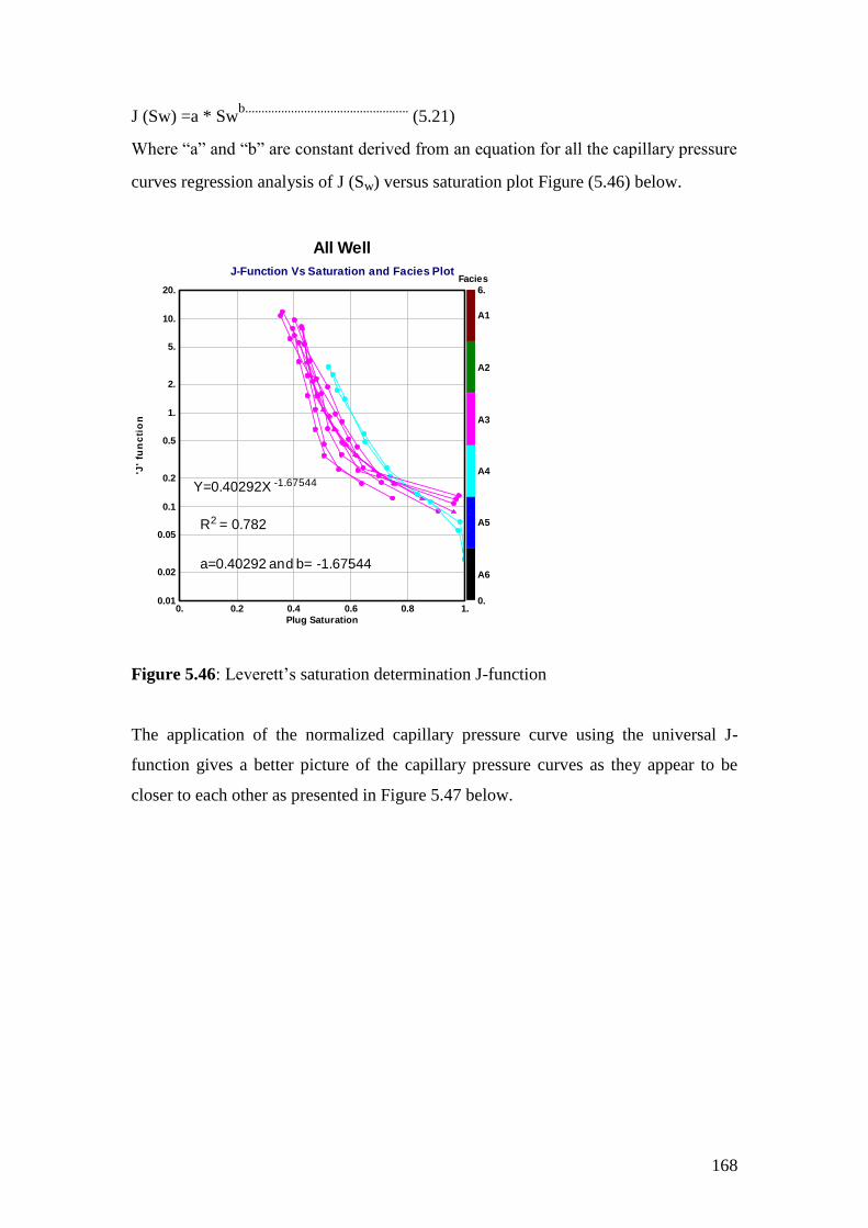
168

J (Sw) =a * Swb..................................................

(5.21)

Where “a” and “b” are constant derived from an equation for all the capillary pressure

curves regression analysis of J (Sw) versus saturation plot Figure (5.46) below.

All Well

J-Function Vs Saturation and Facies Plot

0. 0.2 0.4 0.6 0.8 1.

Plug Saturation

0.01

0.02

0.05

0.1

0.2

0.5

1.

2.

5.

10.

20.

'J'

fun

cti

on

A6

A5

A4

A3

A2

A1

0.

6.

Facies

Y=0.40292X -1.67544

R2 = 0.782

a=0.40292 and b= -1.67544

Figure 5.46: Leverett‟s saturation determination J-function

The application of the normalized capillary pressure curve using the universal J-

function gives a better picture of the capillary pressure curves as they appear to be

closer to each other as presented in Figure 5.47 below.

169

Well OP1

J-Function Vs Saturation and facies

0. 0.2 0.4 0.6 0.8 1.


0.01

3.208

6.406

9.604

12.802

16.

'J'

fun

cti

on

A6

A5

A4

A3

A2

A1

0.

6.

Facies

Well OP3

J-Function Vs Saturation and facies

0. 0.2 0.4 0.6 0.8 1.


0.01

3.208

6.406

9.604

12.802

16.

'J'

fun

cti

on

A6

A5

A4

A3

A2

A1

0.

6.

Facies

Figure 5.47: J-function curves for well OP1 and OP3

The saturation-height function have been established from the capillary pressure data

using the J-function technique for estimated water saturation from height, porosity,

and permeability as presented in Figure 5.48 .

Figure 5.48: Saturation-height function for wells OP1 and OP3

Well OP1 and OP3

Saturation-Height Plot

0. 0.2 0.4 0.6 0.8 1.


0.

80.

160.

240.

320.

400.

He

igh

t (M

)

A6

A5

A4

A3

A2

A1

0.

6.

Facies

GWC = 12.6mFWL

170

The free water level is the point where the brine is completely saturated and the

capillary pressure at that particular point is at zero psi. A possible gas water contact

(GWC) of about 12.6 m was estimated in the saturation-height plot of Figure 5.48

above. Facies A3 presents smaller separation between the gas water contact point as

compared to facies A4 and the reason for this may be attributed to the higher

permeability values in the facies.

171

CHAPTER SIX

PETROPHYSICAL MODEL OF VOLUME OF SHALE, POROSITY

AND WATER SATURATION FROM CORE AND LOG

6.1 INTRODUCTION

The static reservoir modelling involves the integration of core data, log and

engineering data which are used in order to understand the behaviour of the reservoir

at in situ condition. The goal of this chapter is to incorporate core description and

analysis data of the key wells (OP1, OP2 and OP3) into log analysis models of

volume of shale, porosity and water saturation for uncored intervals and field study.

6.2 VOLUME OF SHALE MODEL

The volume of shale (Vsh) quantity is defined as the volume of wetted shale per unit

volume of reservoir rock. Wetted shale is the space occupied by water confined to the

shale known as bound water. A shale can be described by listing some of its attributes

as presented by Holt & Olav-Magnar (2008) .Shale can be regarded clay minerals

that constitute the load bearing framework and shale‟s have nannometer pore sizes

and nanno-darcy permeability; surface area is large ,and water is absorbed on surfaces

or bound inside clay platelets (Keith, 2008). The difference in rock properties can be

used to distinguish sands from shale as presented by Heslop in Figure 6.1a below.

Figure 6.1a: Schematic diagram of variation of sediments with clay mineral content

increasing from left to right (modified after Heslop, 1972).

172

Figure (6.1a) above shows what happens as clay content is increased from clean

sandstones on the left to clay rich shale on the right. In the sands on the left, stresses

are supported by rigid sand grains and grain contacts. Small amounts of clay are

accommodated in the intergranular spaces and do not support external stress. With

increasing clay, eventually the sand and silt grains cannot form a continuous network

with stresses supported by grain-grain contacts and the grains then float in a clay

mineral matrix that is load bearing. Heslop used the gamma ray (GR) log response as

a means of clay content.

Shaly sands are sands with a shale component. These shales are very significant

component of shaly sand reservoirs. Increased volumes of shale decrease the effective

reservoir capacity and conductive shales reduce the formation resistivity and if not

corrected for, give wrong volume of hydrocarbon calculations (Kenneth & Alan

Heslop, 2003). The volume of shale need to be calculated in petrophysical evaluation

in order to correct porosity and water saturation results for the biased effects of shale.

The volume of shale is considered as an indicator for reservoir quality. In addition to

the shale volume, it is important to determine the types of shale for choosing the

appropriate shale model which can be utilized for selecting suitable models.

The shale content is determined using different shale indicators. The following

methods were used to define the shale volume in this study:

Gamma-Ray (GR) log

Spontaneous Potential (SP) log

Neutron log

Resistivity logs

Double clay indicators:

Neuron/Density

Sonic / Density

Neutron/Sonic

The estimated volume of shale determined from log will be compared with clay

volume determined from petrography analysis (X-Ray Diffraction) data acquired from

core samples in wells.

173

6.2.1 Gamma-Ray Method

The gamma ray log is the most common shale volume indicator. The log responds to

the changes in natural radiation emitted by formation. In shaly sands the level of

gamma radiation emitted is a function of clay volume. The gamma ray log does not

measure the volume of silts or other inclusions within the shales. The maximum

gamma ray response is taken as the shale point and minimum response as the clean

sand point.

The Gamma-Ray clay indicator can be calculated using the following methods

(Dresser Atlas, 1979).

Linear Method:

Volume of Shale (Vsh) = GR value (log) – GR (min) ……………….. (6.1)

GR (max) - GR (min)

Where

GR value (log) = GR log value reading of formation to be evaluated

GR (min) = Clean formation

GR (max) = GR value of maximum shale reading in the formation

Non linear Gamma- Ray Method:

Z = Calculated volume of shale = Vsh

Let Z = Vsh as discussed in linear method above

If Z is less than 0.55

Vsh = 0.0006078 * (100 * Z) 158527

If 0.73 < Z > 0.55

Vsh = 2.1212 * Z - 0.81667

If 1.0 < Z > 0.73

Z = Vsh

174

6.2.2 Spontaneous Potential (SP) Method

The volume of shale (Vsh) could be determined from the spontaneous potential (SP)

log using the following relationship.

Vsh = SPclean – SPlog ……………………………. (6.2)

SPclean - SPshale

Where:

Vsh = Volume of shale or clay

SPlog = SP in the zone of interest (read from log)

SPclean = Maximum SP deflection from a nearby clean wet zone in the same Well.

SPshale = SP value in a shale (assumed to be zero)

6.2.3 Neutron Log Method

The neutron log measures the hydrogen content of formation. It records a nearly

constant response through sand formations and increases in shales.

This method can be used for determining the shale volume in case of high clay

content and low effective porosity from the relationship below:

Vsh = ( Фneu * Фneu - Фneu clean ) 0.5

Фneuclay Фneuclay – Фneu clean …………….. (6.3)

Or

Vsh ≤ Фnlog

Фnsh

Where:

Фnlog = the neutron log reading of study zone

Фnsh = neutron log reading in front of a shaly zone

175

6.2.4 Resistivity Method

This method can be used to calculate the shale volume in case of high clay content

and low true resistivity (Rt) values from the relationships below:

Vsh ≤ Rsh

Rt

If this ratio is less than 0.5 then:

Z = Rclay * ( Rclean - Rt )………………….. (6.4)

Rt (Rclean – Rclay)

If Rt is greater than 2 Rclay then

Vsh = 0.5 * (2 * Z) 0.67 * (Z+ 1)

Otherwise Vsh= Z

Where

Rclay = resistivity log reading of a shaly zone

Rsh = Resistivity of the adjacent shale unit

Rclean = Resistivity of a clean formation

6.2.5 Correction of Shale Volume

The values of Z or Vsh calculated above have to be corrected to obtain the optimum

shale values suitable in log interpretation. The formulae are as follows:

Clavier (Clavier et al, 1971):

Vsh = 1.7 (3.38 * (Z + 0.7)2 ) 0.5

Larionov (Tertiary rocks)

Vsh = 0.33 ( 22*Z

- 1)

Steiber( Steiber,1973):

Vsh = 0.5 * Z

1.5 - Z

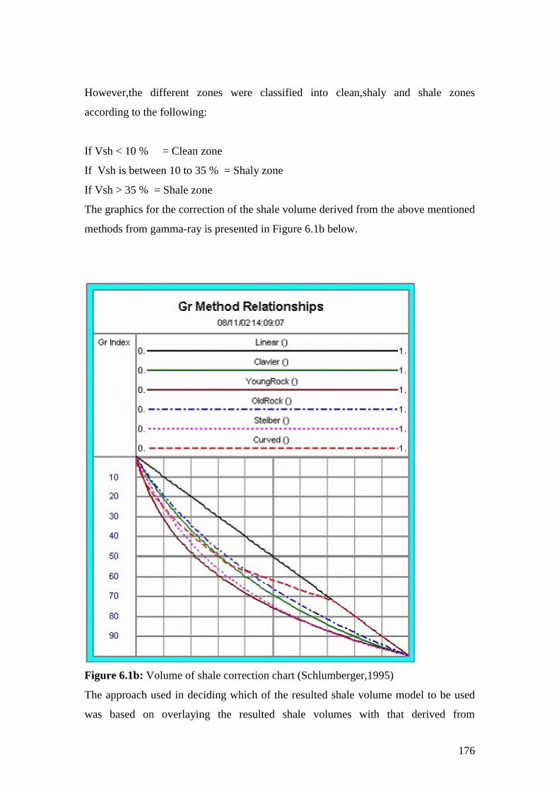
176

However,the different zones were classified into clean,shaly and shale zones

according to the following:

If Vsh < 10 % = Clean zone

If Vsh is between 10 to 35 % = Shaly zone

If Vsh > 35 % = Shale zone

The graphics for the correction of the shale volume derived from the above mentioned

methods from gamma-ray is presented in Figure 6.1b below.

Figure 6.1b: Volume of shale correction chart (Schlumberger,1995)

The approach used in deciding which of the resulted shale volume model to be used

was based on overlaying the resulted shale volumes with that derived from

177

petrography studies. The best match with the petrography volume of shale was

choosen.

6.2.6 Double Clay Indicators

The double clay indicators utilize the principle of defining a clean line and a clay

point. The clay volume is calculated as the distance the input data falls between the

clay point and the clean line. An example of double clay indicator is shown in Figure

6.2 below.

Figure 6.2: Example of neutron-density cross plot as clay indicator

The double clay indicators equations are given below:

The Neutron-Density double clay indicator relationship:

Vsh = ( Dencl2 – Dencl1) * ( Neu – Neu cl 1) –(Den –Den cl1) * (Neu cl2 – Neucl1)

(Dencl2-Dencl1) * (Neuclay-Neucl1) – (Denclay –Dencl1) *(Neucl2 –Neucl1)

Where

Dencl1, Neucl1, Dencl2 and Neucl2 are the density and neutron values for the two

ends of the clean line.

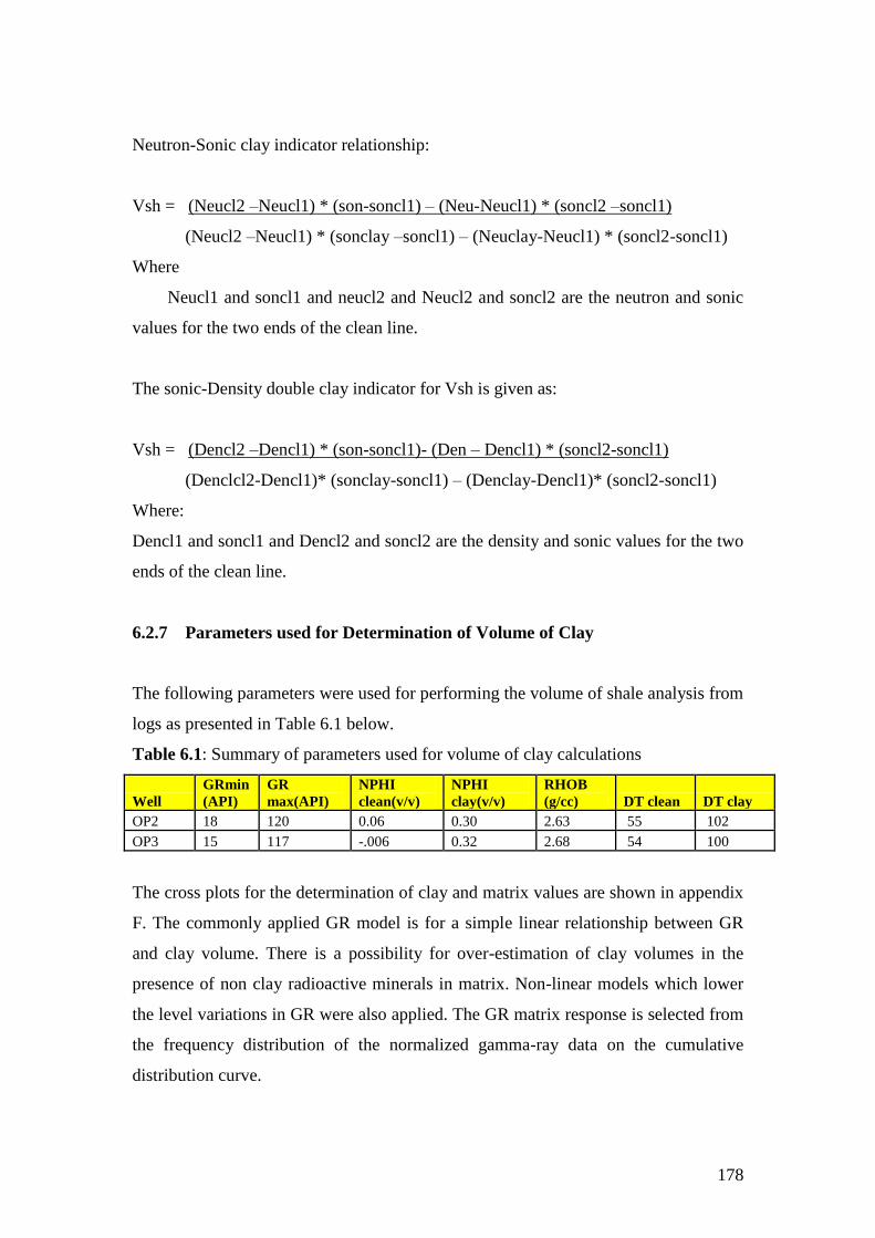
178

Neutron-Sonic clay indicator relationship:

Vsh = (Neucl2 –Neucl1) * (son-soncl1) – (Neu-Neucl1) * (soncl2 –soncl1)

(Neucl2 –Neucl1) * (sonclay –soncl1) – (Neuclay-Neucl1) * (soncl2-soncl1)

Where

Neucl1 and soncl1 and neucl2 and Neucl2 and soncl2 are the neutron and sonic

values for the two ends of the clean line.

The sonic-Density double clay indicator for Vsh is given as:

Vsh = (Dencl2 –Dencl1) * (son-soncl1)- (Den – Dencl1) * (soncl2-soncl1)

(Denclcl2-Dencl1)* (sonclay-soncl1) – (Denclay-Dencl1)* (soncl2-soncl1)

Where:

Dencl1 and soncl1 and Dencl2 and soncl2 are the density and sonic values for the two

ends of the clean line.

6.2.7 Parameters used for Determination of Volume of Clay

The following parameters were used for performing the volume of shale analysis from

logs as presented in Table 6.1 below.

Table 6.1: Summary of parameters used for volume of clay calculations

Well

GRmin

(API)

GR

max(API)

NPHI

clean(v/v)

NPHI

clay(v/v)

RHOB

(g/cc) DT clean DT clay

OP2 18 120 0.06 0.30 2.63 55 102

OP3 15 117 -.006 0.32 2.68 54 100

The cross plots for the determination of clay and matrix values are shown in appendix

F. The commonly applied GR model is for a simple linear relationship between GR

and clay volume. There is a possibility for over-estimation of clay volumes in the

presence of non clay radioactive minerals in matrix. Non-linear models which lower

the level variations in GR were also applied. The GR matrix response is selected from

the frequency distribution of the normalized gamma-ray data on the cumulative

distribution curve.

179

The density of clay was estimated from the Density-Gamma-Ray cross plot and wet

clay properties were established from the Neutron-Density cross-plot as presented in

the appendix I. The DT matrix (clean) and clay were selected from the frequency

distribution of the sonic log data on the cumulative distribution and cross-plots with

gamma-ray log.

6.2.8 Calibration of Volume of Clay (Vcl) Models

This part of the study deals with the integration of the quantitative mineralogy results

obtained from X-Ray analysis (XRD) with wireline logs. The mineralogy results were

presented in chapter four (5) were correlated with the wireline logs for wells OP2 and

OP3. Evaluations of logs produce proportions by volume so the XRD results have

been converted to proportion by volume based on the relationship below:

Weight Volume % of rock = (Dry weight %)*( 1 – Porosity)* (Rock Grain Density)

Mineral Grain Density

Where:

Dry weight % = Dry weight percentage of rock in percent

Porosity = Porosity from routine core analysis in fractions

Rock Grain density = Routine core grain density in g/cc

Mineral Grain density = Fixed mineral for a particular mineral and taken from

standard log chart reference Tables or book.

The volume of clay models derived from logs have been assessed against the

independent X-ray diffraction (XRD) data acquired in well OP2 and OP3. The XRD

data have been converted to proportion by volume since evaluations from logs

generate proportions by volume.

Presented in Figures 6.3 and 6.4 below are the models of clay volumes from based on

logs been overlaid XRD clay volume on each other.

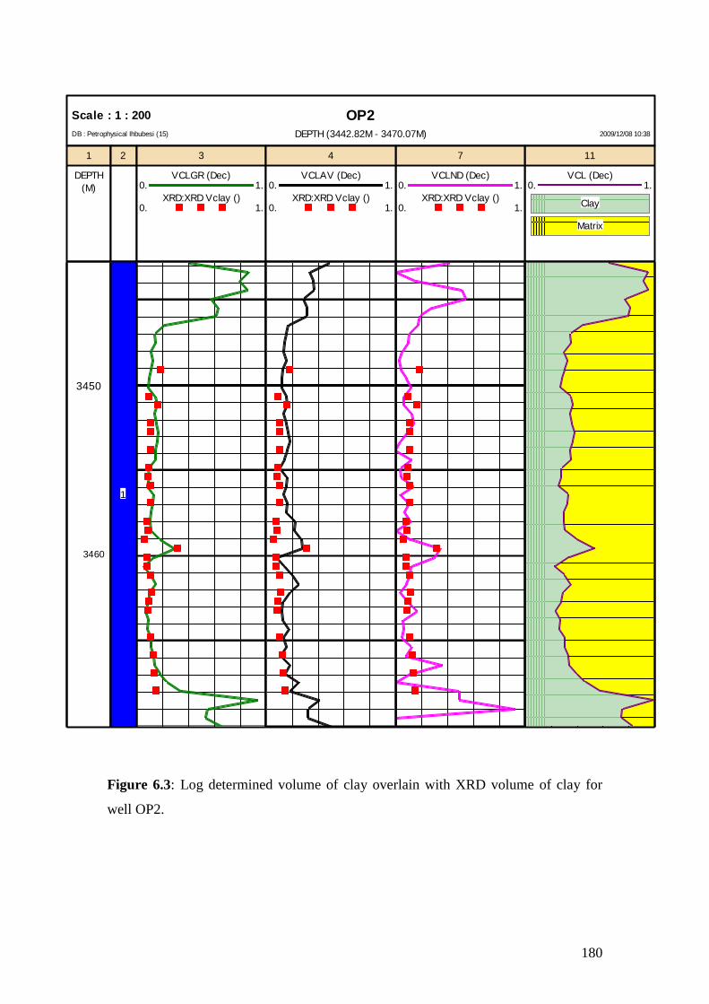
180

Figure 6.3: Log determined volume of clay overlain with XRD volume of clay for

well OP2.

OP2Scale : 1 : 200


1

DEPTH

(M)

2 3

VCLGR (Dec)0. 1.

XRD:XRD Vclay ()0. 1.

11

VCL (Dec)0. 1.

Clay

Matrix

7

VCLND (Dec)0. 1.


4

VCLAV (Dec)0. 1.


3450

1

3460

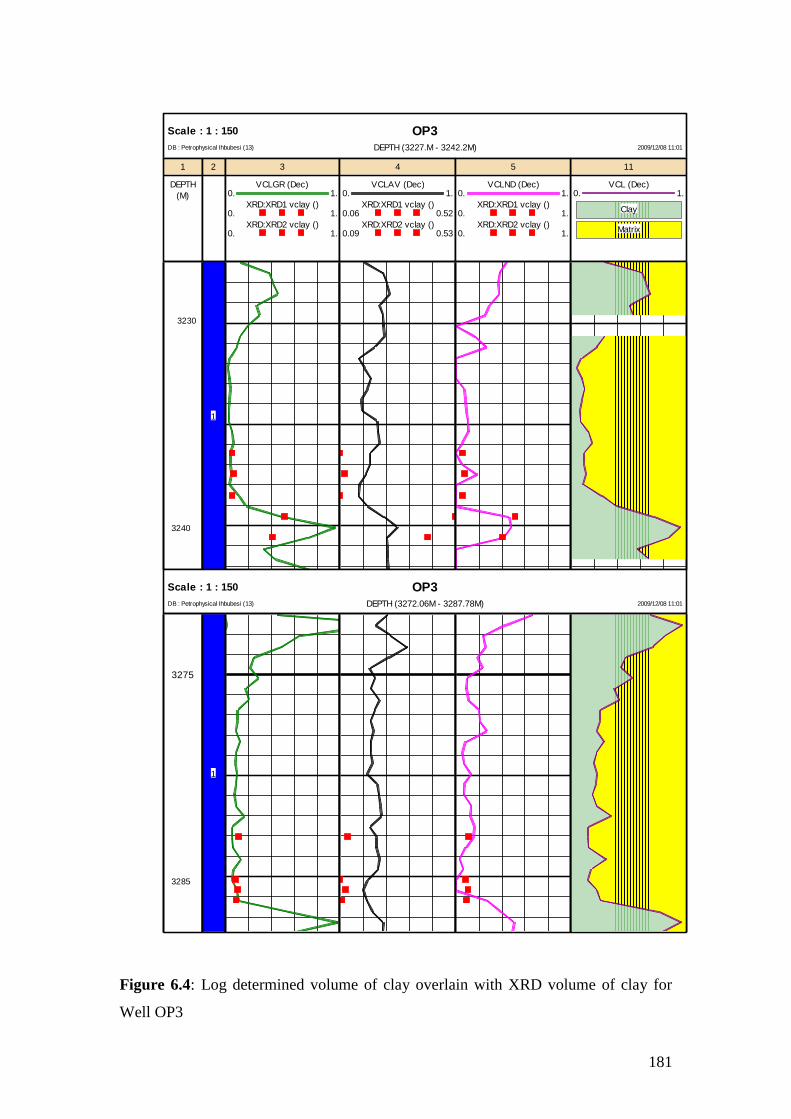
181

Figure 6.4: Log determined volume of clay overlain with XRD volume of clay for

Well OP3

OP3Scale : 1 : 150


1

DEPTH

(M)

2 3

VCLGR (Dec)0. 1.

XRD:XRD1 vclay ()0. 1.


11

VCL (Dec)0. 1.

Clay

Matrix

4

VCLAV (Dec)0. 1.

XRD:XRD1 vclay ()0.06 0.52

XRD:XRD2 vclay ()0.09 0.53

5

VCLND (Dec)0. 1.



1

OP3Scale : 1 : 150


3275

1

3240

3230

3285

182

In both plots of Figures 6.2 and 6.3 above, the volume of clay derived from the XRD

is plotted on the red dot lain against the well derived volume of clay models from

logs. The green coloured curves are the volume of clay from gamma-ray non-linear

model (Steiber VCLGR); the pink coloured are the volume of clay from the double

clay Neutron-Density (VCLND) model; and black colour represents the average

volume of clay (VCLAV) from all the log models.

The linear Gamma-ray model over-estimated the initial volume of clay calculated,

therefore the Larinov, Clavier and Steiber non-linear model was adopted and the

Steiber model was observed to be more compatible with the XRD volume of clay

model in both Wells.

Another log volume of clay model that generates clay volume that was compatible

with the XRD model was the Neutron-Density model. The model has its limitations in

that it may under-estimate clay volumes in the presence of light hydrocarbons such as

gas and may also over-estimate clay volumes where carbonate cements or heavy

minerals are present. The XRD data indicate no significant carbonate and heavy

minerals such as pyrite and siderite so the Neutron-Density model volume of clay was

Not over-estimated. Well OP2 Neutron-Density volume of clay model is more

compatible with the XRD volume of clay than in well OP2.

There exist significant scale similarities between the XRD volume of clay and the log

derived volume of clay in the gamma-ray and N-D double clay models in both wells

in the level of clay. The volume of clay from the resistivity log and the averaged

volume of clay from logs indicate significantly higher clay volumes than the XRD and

hence will not be used for the final volume of clay model.

The final volume of clay model from logs is taken from the gamma-ray model

corrected by Steiber equation. This is based on the observed higher levels of

agreement between the log and XRD volume of clay data as shown in the plots of

both wells.

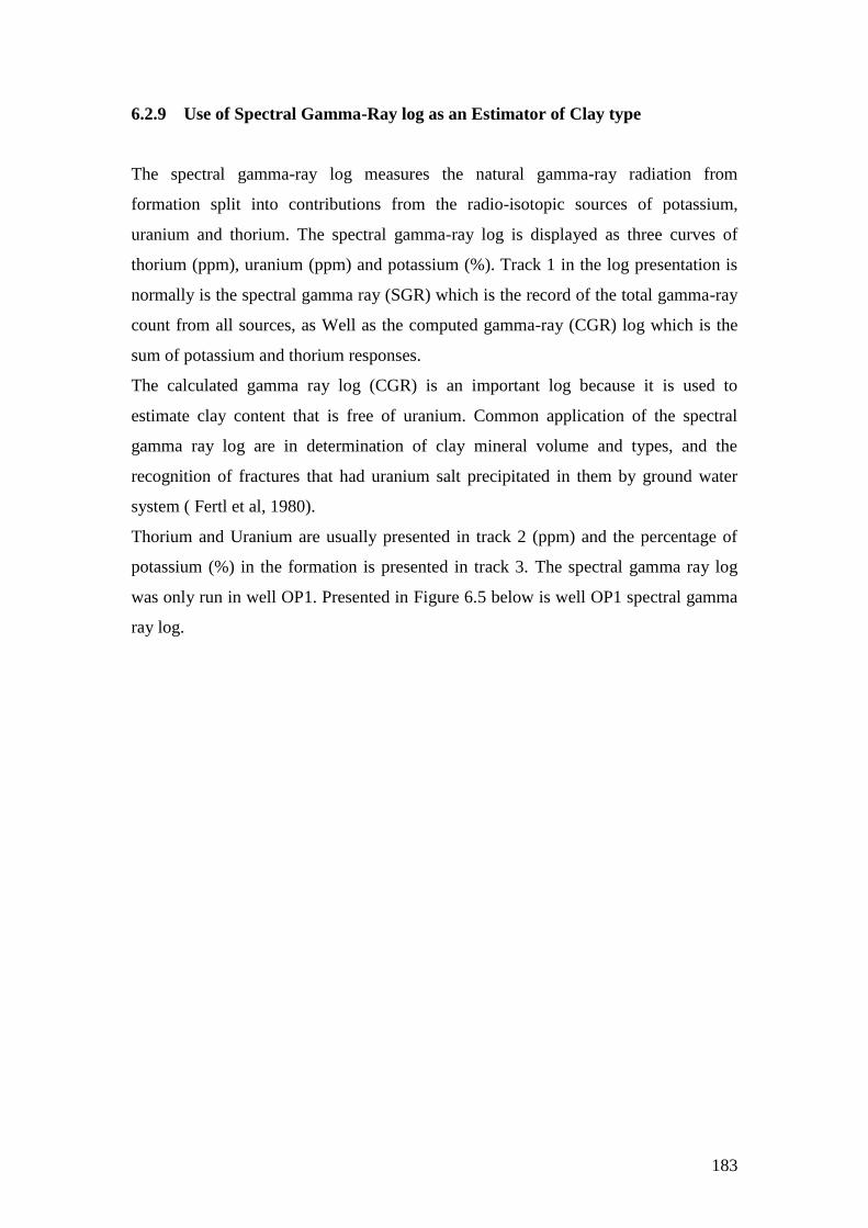
183

6.2.9 Use of Spectral Gamma-Ray log as an Estimator of Clay type

The spectral gamma-ray log measures the natural gamma-ray radiation from

formation split into contributions from the radio-isotopic sources of potassium,

uranium and thorium. The spectral gamma-ray log is displayed as three curves of

thorium (ppm), uranium (ppm) and potassium (%). Track 1 in the log presentation is

normally is the spectral gamma ray (SGR) which is the record of the total gamma-ray

count from all sources, as Well as the computed gamma-ray (CGR) log which is the

sum of potassium and thorium responses.

The calculated gamma ray log (CGR) is an important log because it is used to

estimate clay content that is free of uranium. Common application of the spectral

gamma ray log are in determination of clay mineral volume and types, and the

recognition of fractures that had uranium salt precipitated in them by ground water

system ( Fertl et al, 1980).

Thorium and Uranium are usually presented in track 2 (ppm) and the percentage of

potassium (%) in the formation is presented in track 3. The spectral gamma ray log

was only run in well OP1. Presented in Figure 6.5 below is well OP1 spectral gamma

ray log.

184

OP1Scale : 1 : 150


1

DEPTH

(M)

Total Gamma-Ray

SGR (GAPI)0. 150.

CGR (GAPI)0. 150.

Thorium

THOR (PPM)0. 20.

Potassium and Uranium

URAN (PPM)0. 20.

POTA (%)0. 0.5

Lithology

VWCL (Dec)0. 1.

Clay

Sandstone

3375

3370 SGR

CGR

Figure 6.5: Well OP1 spectral gamma ray log

Figure 6.5 above showed an average concentration of thorium within the reservoir

interval of well OP1 of approximately 7 ppm, uranium 2 ppm, and potassium 0.03 %.

The low percentage of potassium within the reservoir area is as expected because the

whole rock analysis results of adjacent wells showed insignificant percentage of

potassium feldspar. This shows that sandstones in the reservoir intervals do not

contain feldspars, micas, glauconite, and heavy minerals (Tables 5.23 and 5.24).

Clay bearing sandstones and types of clay minerals may be identified by the

potassium-thorium cross plot. Illite clay mineral has higher potassium than mixed-

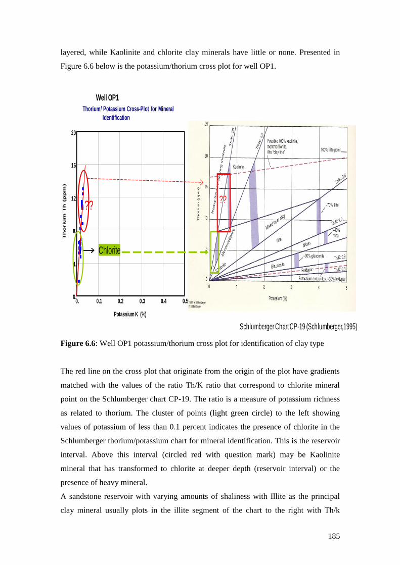
185

layered, while Kaolinite and chlorite clay minerals have little or none. Presented in

Figure 6.6 below is the potassium/thorium cross plot for well OP1.

Well OP1

Thorium/ Potassium Cross-Plot for Mineral

Identification

0. 0.1 0.2 0.3 0.4 0.5

Potassium K (%)

0.

4.

8.

12.

16.

20.

Th

oriu

m T

h (p

pm

)

Chlorite

Schlumberger Chart CP-19 (Schlumberger,1995)

????

Figure 6.6: Well OP1 potassium/thorium cross plot for identification of clay type

The red line on the cross plot that originate from the origin of the plot have gradients

matched with the values of the ratio Th/K ratio that correspond to chlorite mineral

point on the Schlumberger chart CP-19. The ratio is a measure of potassium richness

as related to thorium. The cluster of points (light green circle) to the left showing

values of potassium of less than 0.1 percent indicates the presence of chlorite in the

Schlumberger thorium/potassium chart for mineral identification. This is the reservoir

interval. Above this interval (circled red with question mark) may be Kaolinite

mineral that has transformed to chlorite at deeper depth (reservoir interval) or the

presence of heavy mineral.

A sandstone reservoir with varying amounts of shaliness with Illite as the principal

clay mineral usually plots in the illite segment of the chart to the right with Th/k

186

between 2.0 and 2.5. Less shaly parts of the reservoir plot closer to the origin and

more shaly parts plot closer to the 70 % illite area of the chart (Schlumberger, 1995).

6.3 POROSITY MODEL

The porosity of a rock is the volume of the non-solid portion of the rock that is filled

with fluids divided by the total volume of the rock. Porosity is considered to be a

primary porosity if it is developed during the original sedimentation process by which

the rock is created. Secondary porosity is created by processes which synthesize vugs

in rocks by ground water (Crain, 1986).In general, porosities tend to be lower in

deeper and older rocks due to cementation and overburden pressure stress on the rock.

The porosity from logs can be estimated from a single porosity log (density, neutron,

sonic) or a combination of porosity logs. The porosity derived directly from logs

without correction for clay content is regarded as total porosity. Effective porosity is

the resultant porosity determined after removal of the effect of clay. However, in an

interval of no shale, the total porosity equals the effective porosity.

Estimation of porosities from wireline logs requires information on lithology, core

data which includes grain matrix and pore fluid. The porosity from log can be

determined in both clean and shaly zones as presented below.

6.3.1 Porosity Determination from Density Log

The porosity derived from the density log (ΦD) is defined by the following

relationships (Wyllie, 1963).

Porosity (ΦD) = (ρma - ρb) …………………………………………….. (6.5)

(ρma - ρf)

Where:

ρma = matrix (or grain) density= 2.67g/cc from core.

ρb = Bulk density as measured by the tool

ρf = Fluid density (derived from pressure test ). Field water density of 1.02 g/cc and

gas density of 0.2 g/cc.

187

For:

Fresh water mud, ρf = 1.0 g/cm3

Salt water mud, ρf = 1.1 g/cm3

Gas mud, ρf = 0.7 g/cm3

According to Dresser Atlas 1979, density porosity in a shaly formation is calculated

using the following equation:

ΦD corr = ( ρma - ρb ) - Vsh (ρma - ρsh ) …………………………….... (6.6)

(ρma - ρf ) ( ρma - ρf )

Where:

ΦD corr = Corrected density for shale effect

Vsh = Volume of shale

ρsh = Density value of adjacent shale formation

6.3.2 Porosity from Neutron Log

Neutron log porosity is calculated by the acquisition software and is displayed directly

on the log (Krygowski, 2003). The logs must be interpreted from a specific chart

because they are not calibrated in physical units. A convenient standard for the

neutron log is the neutron porosity index given in limestone.

In a shaly formation, the neutron log will appear to be more porous. The effect of

shale on the neutron log can be corrected by the following equation:

ΦNcorr = ΦNlog - Vsh X ΦNsh ………………………………………………. (6.7)

Where

ΦNcorr = Corrected neutron porosity

ΦNlog = Neutron log reading of the interval


ΦNsh = neutron log of the adjacent shale formation

188

6.3.3 Porosity from Sonic (acoustic) Log (ΦS)

The acoustic travel time is a function of the formation lithology and porosity. The

following equations are used to calculate the sonic porosity in consolidated and

compacted formations (Wyllie et al, 1958).

Wyllie Time – Average Equation:

ΦS = DT - DT Ma * 1 …………………………………..(6.8)

DT Fl - DTMa Bcp

Where:

ΦS = Sonic (acoustic) porosity

DT = Sonic travel time from the log

DTMa = Matrix travel time

Bcp = compaction correction = DTShale > 1.0

100

Raymer-Hunt Gardner (1980) equation:

ΦS = 5 * DT - DTMa …………………………….. (6.9)

8 DT

Hilchie, 1978 suggested the following empirical correction for the hydrocarbon

effects on sonic derived porosity in a gas formation:

Φcorr = Φsonic * 0.7 …………………………………. (6.10)

However, a combination of any of the two porosity logs can be used to determine

porosity in clean and shaly sand environments.

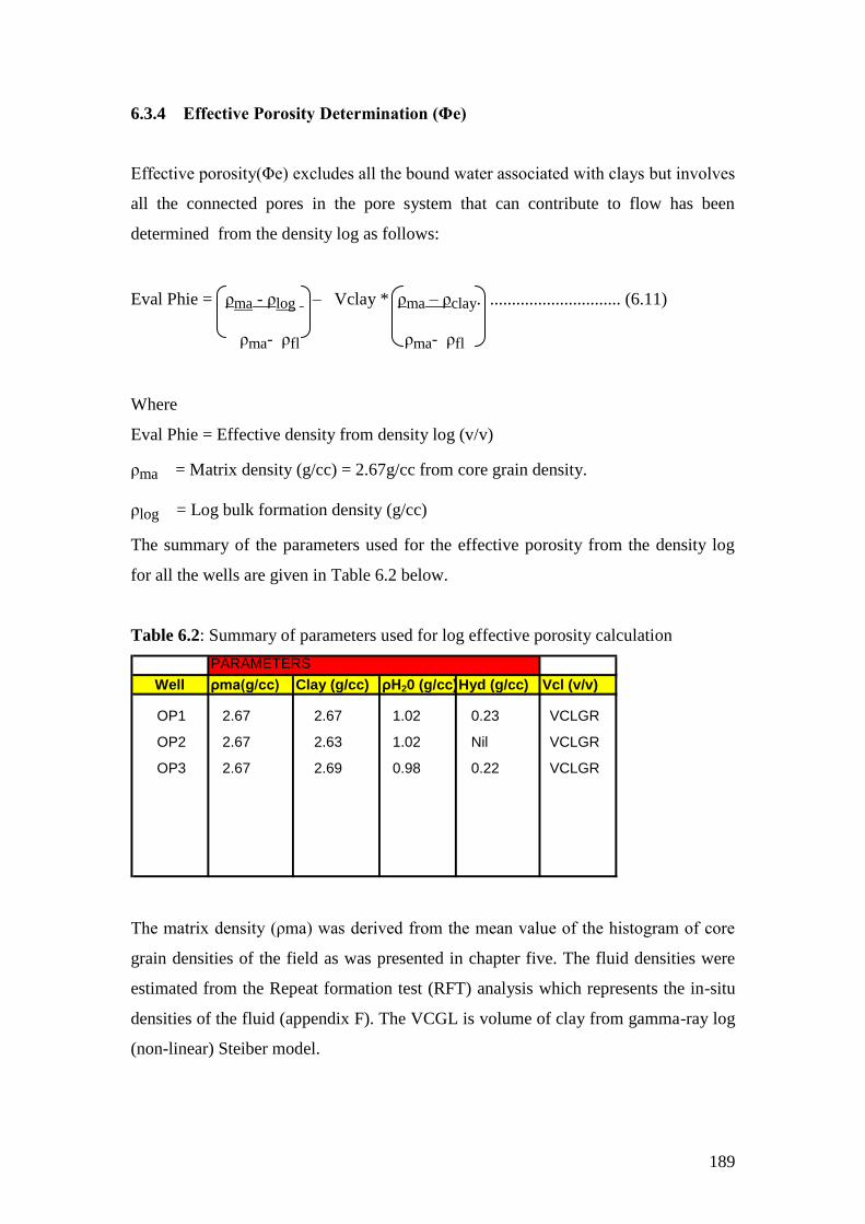
189

6.3.4 Effective Porosity Determination (Φe)

Effective porosity(Φe) excludes all the bound water associated with clays but involves

all the connected pores in the pore system that can contribute to flow has been

determined from the density log as follows:

Eval Phie = ρma - ρlog – Vclay * ρma – ρclay. .............................. (6.11)

ρma- ρfl ρma- ρfl

Where

Eval Phie = Effective density from density log (v/v)

ρma = Matrix density (g/cc) = 2.67g/cc from core grain density.

ρlog = Log bulk formation density (g/cc)

The summary of the parameters used for the effective porosity from the density log

for all the wells are given in Table 6.2 below.

Table 6.2: Summary of parameters used for log effective porosity calculation

The matrix density (ρma) was derived from the mean value of the histogram of core

grain densities of the field as was presented in chapter five. The fluid densities were

estimated from the Repeat formation test (RFT) analysis which represents the in-situ

densities of the fluid (appendix F). The VCGL is volume of clay from gamma-ray log

(non-linear) Steiber model.

PARAMETERS

Well ρma(g/cc) Clay (g/cc) ρH20 (g/cc) Hyd (g/cc) Vcl (v/v)

OP1 2.67 2.67 1.02 0.23 VCLGR

OP2 2.67 2.63 1.02 Nil VCLGR

OP3 2.67 2.69 0.98 0.22 VCLGR

190

Gas indication can be determined in the formation by comparison of the corrected

porosity values of neutron and density.

If ΦNcorr is less than ΦD corr then gas is suspected in the formation. The effective

porosity in a shaly sand formation can also be determined from the combination of the

neutron and density porosity logs (John 1983) as follows:

(Φe) = √ ΦD corr 2

+ ΦNcorr 2

/2 …………………………………… (6.12)

6.3.5 Comparison of Log and Core Porosity

The porosities computed from the logs have been calibrated with the overburden

corrected core porosities (ob core). The results when overlaid with the corrected core

data shows that the data sets are generally consistent with one another though there

are cases of discrepancies which may be as a result of the different scales of

measurements and as a result of lithology factor as the routine core measured

porosities are generally lower than the log derived porosities in all wells. The

evaluated effective porosity is also shown in each of the plot tracks as shown in

Figure 6.7 below for well OP1.

191

Figure 6.7: Well OP1 comparison of log and core porosity

Track 5 in Figure 6.7 above present the log derived porosity from the density (Phi-

den) red colour , track 6 is neutron porosity (PhiNeu- green colour), and track 7 is the

sonic porosity (PhiSon- Pink colour ). The porosity logs in their respective tracks

were plotted against the routine core derived porosity (ob-porosity) black dots for

comparison.

The sonic derived porosity and density porosity best compared with the routine core

porosity. The plot for well OP2 is presented in Figure 6.8 below.

OP1Scale : 1 : 200


1

DEPTH

(M)

Gamma-Ray

GR (GAPI)0. 200.

Caliper

CALI6.16.

Porosity Input


DT (US/F)140. 40.

Run2:NPHI (dec)0.45 -0.15

PEFC (B/E)0. 20.

SAND

SHALE

Density Porosity

PhiDen (dec)0.5 0.


Neutron Porosity

PhiNeu (dec)0.5 0.


Sonic Porosity

PhiSon (dec)0.5 0.


Lithology

VCL (Dec)0. 1.

Clay

Matrix

3375

3380

192

Figure 6.8: Well OP2 comparison of log and core porosity.

Plotted in track 5 of Figure 6.8 above is the density porosity log (Phiden-red colour),

track 6 is the neutron porosity log (Phineu-green colour) and track 7 is the sonic

porosity (Phison-pink colour). The log derived porosity curves were overlain with the

routine core porosity for comparison purposes. The porosity derived from the sonic

log best match with the routine core porosity as shown.

The presence of clay and enlarge borehole presents a difficulty because of variability

with respect to concentrations of elements with large thermal neutron absorption cross

section which has a strong effect on the thermal neutron log as shown in the lower

part of the neutron porosity log. The capiler log was introduce in track 4 to check hole

OP2Scale : 1 : 240


1

DEPTH

(M)

Gamma-Ray

GRn (GAPI)0. 150.

Porosity Input


DTCO_E (US/FT)140. 40.

TNPH (V/V)0.45 -0.15

PEFZ (B/E)0. 20.

SAND

SHALE

Caliper

HCA6.16.

Density Porosity

PhiDen (dec)0.5 0.


Neutron Porosity

PhiNeu (dec)0.5 0.


Sonic Porosity

PhiSon (dec)0.5 0.


Lithology

VCL (Dec)0. 1.

Clay

Matrix

3450

3460

3470

193

enlargement. Figure 6.9 below presents the log and core porosity data comparison for

well OP3.

Figure 6.9: Well OP3 comparison of log and core porosity

Two non-continuous core samples were measured in this Well and the porosity results

were compared with the log derived porosity as presented in Figure 6.8 above. Track

5 is the density porosity (Phidensity –red colour), track 6 is the neutron porosity

(Phineu-green colour) and track 7 is the sonic porosity (Phison- Pink colour), all

plotted against the core porosity (ob porosity –black dots) for comparison.

The best match of log derived porosity to routine core porosity were the density

porosity and sonic in core 1. The caliper log was also introduced in track 4 to check

hole enlargement. The effect of clay material on the thermal neutron porosity log was

OP3Scale : 1 : 300


1

DEPTH

(M)

Gamma-Ray

GR (gAPI)0. 150.

Porosity Input

RHOBE (g/cm3)1.95 2.95

DT (US/F)140. 40.

NPHI (m3/m3)0.45 -0.15

SAND

SHALE

Caliper

CALI6.16.

Density Porosity

PhiDen (dec)0.5 0.


Neutron Porosity

PhiNeu (dec)0.5 0.


Sonic Porosity

PhiSon (dec)0.5 0.


Lithology

VCL (DEC)0. 1.

Clay

Matrix

OP3Scale : 1 : 300


3230

3240

3275

3285

194

also observed in the lower section of core 2 of the neutron porosity log as a result of

the discrepancy between both data at clay section.

Generally, the intervals were the log and core porosity shows a departure from each

other is associated with clay materials which may expand slightly because of rebound

effects leading to an increase in volume which causes a decrease in bulk density and

at intervals where there is an increase in hole diameter. The cross plots of log and core

data porosities are shown in appendix G. It could be deduced from the above that the

differences in porosity measurements between core and log may be due to the effect

of authigenic clays which reduce effective porosity at reservoir conditions but caused

an over-estimation of porosity in the air-dried cores measured in the laboratory.

In conclusion, the density and neutron logs have to be corrected for the effect of shale

and the sonic log derived porosity generally showed the best match with the core

derived porosity and hence will be used for the porosity model. An empirical

relationship between the overburden corrected porosity from core and log derived

porosity from the sonic porosity log was established by plotting the overburden

corrected porosity determined in all the Well versus the sonic porosity on a linear

scale. The plot is presented in Figure 6.10 below.

Figure 6.10: Multi-Well overburden porosity versus log porosity

Multi-Well

Overburden Corrected Porosity Vs Sonic Porosity

0. 0.06 0.12 0.18 0.24 0.3

Sonic Log Porosity (v/v)

0.

0.06

0.12

0.18

0.24

0.3

Ov

erb

urd

en

Po

rosit

y (

v/v

)

Ob Porosity = 0.0097 + 0.9263 * PhiSonic

R2= 0.8707

Well

OP1

OP2

OP3

195

A common equation for predicting the overburden porosity in un-cored intervals and

Wells without core was established through the cross plot. A correlation coefficient of

0.87 was realized which shows that an excellent relationship exist between the two

plotted data from the statistical point of view.

The common equation is given in equation 6.13 below:

Overburden Porosity = 0.0097 + 0.9263 * Phisonic ……………………… (6.13)

R2 = 0.8707

Where:

Overburden porosity = Predicted overburden porosity (v/v)

Phisonic = Sonic Porosity (v/v)

6.4 WATER SATURATION MODEL

The saturation of fluid of a reservoir rock is referred to as the percentage of the pore

space filled with a particular fluid, and the sum of all the fluids in the pore spaces

equals one hundred percent. The saturation of water is always part of the fluids that

occupy the pore spaces of reservoir rock.

The water in a reservoir rock at the time of discovery is referred to as connate water

which is derived from the marine environment in which the sediments were first

deposited. The term interstitial water is often used synonymous with connate water

but it could represent water which resulted from compaction of the rock, the expulsion

of water, and from lateral migration (Levorsen, 1967). Both connate and interstitial

water are used to refer to the water present in all oil or gas reservoirs and is

considered residual or irreducible and immobile.

According to Engineering data book of 1977, the water saturation in any given rock

sample depends upon the size of the pores, the distribution of pore sizes in the rock,

and the height of the sample above the water bearing zone. Connate water usually is

in the range of 10 % to 40 % in most rocks which means that it only occupies about

10 to 40 percent of the pore volume of the rock and other fluids (hydrocarbon) occupy

the rest. In general, coarse grained sandstones, vuggy limestones and other rocks with

large pores will have low connate water saturations and fine grained sandstones and

rocks with small pores tend to have relatively high water saturation.

196

The knowledge of the quantity and distribution of different types of water contained

in the interconnected pore spaces of a reservoir is essential for formation evaluation.

Three main water types has been identified as bound, capillary and free waters .The

bound water includes water that is strongly held to the clay mineral surfaces and the

water of hydration associated with the mineral charge balancing cations. The

Capillary water is the immobile water held by capillary forces in regions of micro-

porosity. Free water is water that resides within the macro-porosity region of the

interconnected pore space of a reservoir and is able to flow under an applied pressure

gradient (Newman, 1987).

The water saturation of reservoir rocks can be determined from the following:

Wireline Logs

Core data

Capillary Pressure Measurements

Drill Stem Test (DST)

However, in this part of the analysis and interpretation, emphasis will be on log

derived water saturation models and compared with water saturation models derived

earlier in chapter five from conventional and special core data results and from

production test data.

Determination of water saturation from logs can be grouped into two, namely the

Clean Sand (Shale free) and Shaly-Sand models. The Clean Sand or shale free group

is determined from the Archie‟s relationship while the Shaly-Sand models can further

be sub-divided into two main equation groups according to Petrolog (2006) as

follows:

Group 1: The volume of Shale or Resistivity model:

Simandoux

Modified Simandoux

Poupon Leveaux

Fertl and Hammack

Indonesia

This particular group uses the effective porosity as the input porosity in the water

saturation equation.

197

Group 2: Cation Exchange or Conductivity model

Waxman-Smits

Modified Waxman-Smits

Dual –Water

Juhasz

The group 2 as listed above uses the total porosity values in the water saturation

equation. Before discussing in details the water saturation models, some of the basic

input parameters to these models such as the formation temperature and resistivity of

water at formation temperature will be estimated and verified in as many ways as

possible. Other basic parameters like cementation and saturation exponents (m and n)

earlier determined from special core analysis will be used for the evaluations of water

saturations.

6.4.1 Parameters

6.4.1.1 Formation Temperature Determination

The following equation was used for formation temperature determination.

T2 = D (BHT - T1) + T1 …………………..(6.13)

TD

Where

T2 = Formation Température

D = Log depth

BHT = Bottom hole temperature

T1 = Surface temperature

TD = Total depth

The resistivity of mud filtrate (Rmf) at formation temperature can also be determined

using the following equation:

Rmf2 = Rmf1 (T1 + 6.77) ................................. (6.14)

(T2 + 6.77)

Where

Rmf2 = Resistivity of mud filtrate at formation temperature (ohm-m in oF)

Rmf1 = Known resistivity of mud filtrate at surface temperature (in oF)

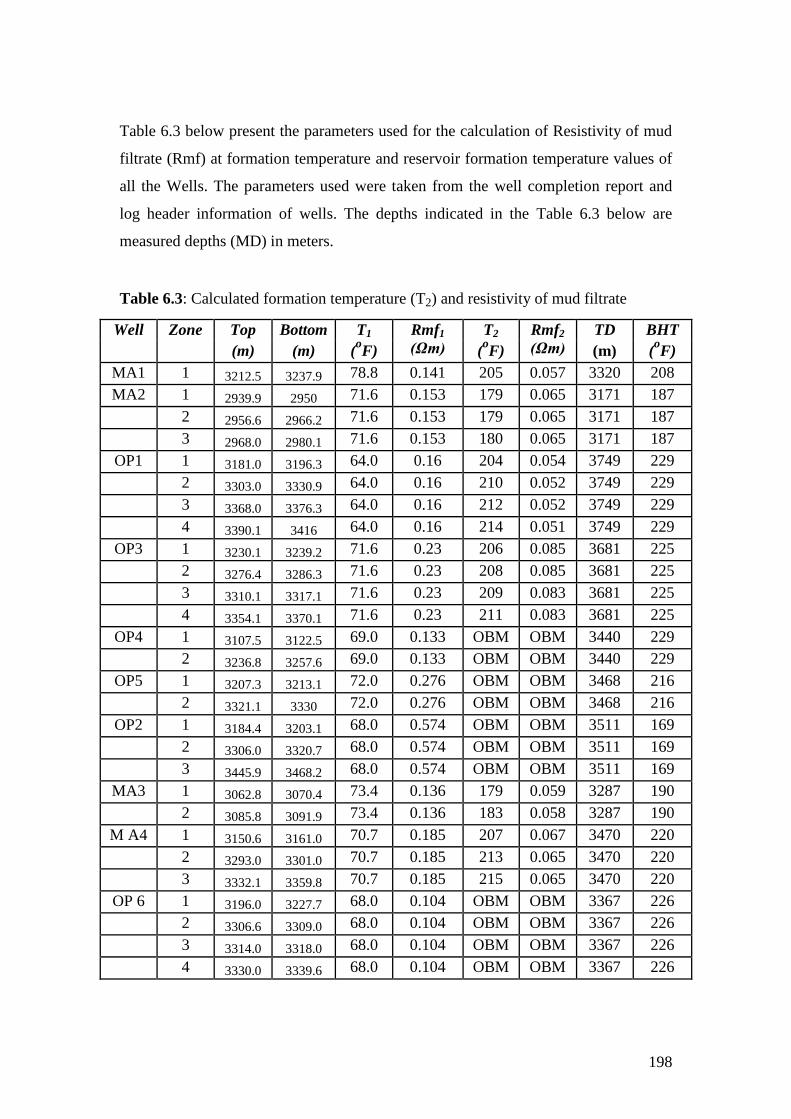
198

Table 6.3 below present the parameters used for the calculation of Resistivity of mud

filtrate (Rmf) at formation temperature and reservoir formation temperature values of

all the Wells. The parameters used were taken from the well completion report and

log header information of wells. The depths indicated in the Table 6.3 below are

measured depths (MD) in meters.

Table 6.3: Calculated formation temperature (T2) and resistivity of mud filtrate

Well Zone Top Bottom T1

(oF)

Rmf1

(Ωm)

T2

(oF)

Rmf2

(Ωm)

TD BHT

(oF) (m) (m) (m)

MA1 1 3212.5 3237.9 78.8 0.141 205 0.057 3320 208

MA2 1 2939.9 2950 71.6 0.153 179 0.065 3171 187

2 2956.6 2966.2 71.6 0.153 179 0.065 3171 187

3 2968.0 2980.1 71.6 0.153 180 0.065 3171 187

OP1 1 3181.0 3196.3 64.0 0.16 204 0.054 3749 229

2 3303.0 3330.9 64.0 0.16 210 0.052 3749 229

3 3368.0 3376.3 64.0 0.16 212 0.052 3749 229

4 3390.1 3416 64.0 0.16 214 0.051 3749 229

OP3 1 3230.1 3239.2 71.6 0.23 206 0.085 3681 225

2 3276.4 3286.3 71.6 0.23 208 0.085 3681 225

3 3310.1 3317.1 71.6 0.23 209 0.083 3681 225

4 3354.1 3370.1 71.6 0.23 211 0.083 3681 225

OP4 1 3107.5 3122.5 69.0 0.133 OBM OBM 3440 229

2 3236.8 3257.6 69.0 0.133 OBM OBM 3440 229

OP5 1 3207.3 3213.1 72.0 0.276 OBM OBM 3468 216

2 3321.1 3330 72.0 0.276 OBM OBM 3468 216

OP2 1 3184.4 3203.1 68.0 0.574 OBM OBM 3511 169

2 3306.0 3320.7 68.0 0.574 OBM OBM 3511 169

3 3445.9 3468.2 68.0 0.574 OBM OBM 3511 169

MA3 1 3062.8 3070.4 73.4 0.136 179 0.059 3287 190

2 3085.8 3091.9 73.4 0.136 183 0.058 3287 190

M A4 1 3150.6 3161.0 70.7 0.185 207 0.067 3470 220

2 3293.0 3301.0 70.7 0.185 213 0.065 3470 220

3 3332.1 3359.8 70.7 0.185 215 0.065 3470 220

OP 6 1 3196.0 3227.7 68.0 0.104 OBM OBM 3367 226

2 3306.6 3309.0 68.0 0.104 OBM OBM 3367 226

3 3314.0 3318.0 68.0 0.104 OBM OBM 3367 226

4 3330.0 3339.6 68.0 0.104 OBM OBM 3367 226

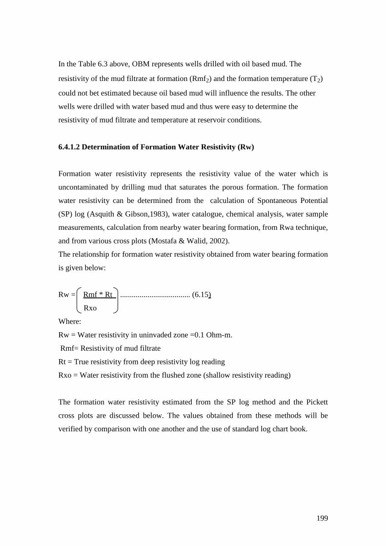
199

In the Table 6.3 above, OBM represents wells drilled with oil based mud. The

resistivity of the mud filtrate at formation (Rmf2) and the formation temperature (T2)

could not bet estimated because oil based mud will influence the results. The other

wells were drilled with water based mud and thus were easy to determine the

resistivity of mud filtrate and temperature at reservoir conditions.

6.4.1.2 Determination of Formation Water Resistivity (Rw)

Formation water resistivity represents the resistivity value of the water which is

uncontaminated by drilling mud that saturates the porous formation. The formation

water resistivity can be determined from the calculation of Spontaneous Potential

(SP) log (Asquith & Gibson,1983), water catalogue, chemical analysis, water sample

measurements, calculation from nearby water bearing formation, from Rwa technique,

and from various cross plots (Mostafa & Walid, 2002).

The relationship for formation water resistivity obtained from water bearing formation

is given below:

Rw = Rmf * Rt .................................... (6.15)

Rxo

Where:

Rw = Water resistivity in uninvaded zone =0.1 Ohm-m.

Rmf= Resistivity of mud filtrate

Rt = True resistivity from deep resistivity log reading

Rxo = Water resistivity from the flushed zone (shallow resistivity reading)

The formation water resistivity estimated from the SP log method and the Pickett

cross plots are discussed below. The values obtained from these methods will be

verified by comparison with one another and the use of standard log chart book.

200

6.4.1.2.1 SP Method for Formation Resistivity Water Estimation

The water formation resistivity value can be estimated from the static spontaneous

potential of the SP log in water bearing clean sand. The baseline shift is first applied

to the SP curve with a shale baseline set to 0.0mV. A formation temperature curve is

entered if available otherwise it is created using the temperature gradient module of

the IP software package.

The result (resistivity of water from SP curve RwSP) curve is then calculated and

corrected to the output temperature entered. Also created is the equivalent salinity of

the RwSP results to salinity in units of Kppm Nacl equivalent. The equation used for

SP water resistivity calculations are given below:

ESSP = - Kc log Rmfeq / Rw …………………………………….. (6.16)

Where

ESSP = Static SP. in mV.

Kc = Temperature of formation

Rmfeq = Equivalent Resistivity of mud filtrate

Rwe = Resistivity of formation water.

K c= temperature dependent factor=65+0.24 * oC =61.3 + 0.133F

This method may not be successfully being applied to Wells drilled with an oil based

mud because sufficient SP will not be generated. Also in shaly formations and

hydrocarbon bearing intervals, SP measurements will be reduced and therefore for the

determination of formation water resistivity, SP is determined in a clean water bearing

sands (Bateman, 1985).

This method was not applied to the oil based mud (OBM) wells. The SP and

temperature logs were not run in some of the wells in the study area; therefore it could

not be used for comparison purposes. Porosity and deep resistivity logs were run in all

wells; therefore the Pickett plot method for water resistivity determination was used

for the determination of resistivity of water and compared with other methods and

standard log chart book.

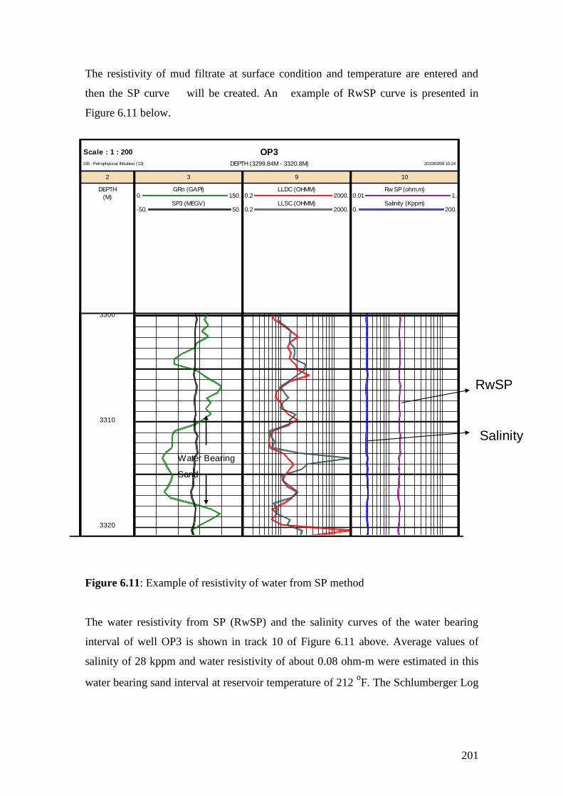
201

The resistivity of mud filtrate at surface condition and temperature are entered and

then the SP curve will be created. An example of RwSP curve is presented in

Figure 6.11 below.

Figure 6.11: Example of resistivity of water from SP method

The water resistivity from SP (RwSP) and the salinity curves of the water bearing

interval of well OP3 is shown in track 10 of Figure 6.11 above. Average values of

salinity of 28 kppm and water resistivity of about 0.08 ohm-m were estimated in this

water bearing sand interval at reservoir temperature of 212 oF. The Schlumberger Log

OP3Scale : 1 : 200


2

DEPTH

(M)

3

GRn (GAPI)0. 150.

SP3 (MEGV)-50. 50.

9

LLDC (OHMM)0.2 2000.

LLSC (OHMM)0.2 2000.

10

Rw SP (ohm.m)0.01 1.

Salinity (Kppm)0. 200.

3300

3310

3320

Facies A3

Facies A4

Facies A5

Facies A6

Facies A4

Facies A3

Facies A6

Water Bearing

Sand

RwSP

Salinity

202

interpretation Chart Gen-9 was used to confirm the salinity and water resistivity

values calculated.

6.4.1.2.2 Pickett Plot method For Formation Water Resistivity Estimation

The concept of the Pickett plot is based on double logarithm plot of a resistivity

measurement on the x-axis versus porosity measurement on the y –axis. After the

points are plotted, the one hundred percent water saturation is fixed by drawing it

through the lowest resistivity points corresponding to different porosities. Points of

constant water saturation will be plotted on straight line and the water resistivity (Rw)

can be determined from point on the straight line (Bate, 1985).

The Pickett plot for water resistivity determination for well OP1, OP2, OP3, and OP4

taken at water bearing intervals is presented in Figure 6.12 below.

Figure 6.12: Pickett Plot for determination of resistivity of water (Rw) for well OP1,

OP2, OP3, and OP4 respectively.

Pickett Plot

Well OP1

0.1 1. 10. 100. 1000.

Resistivity (Ohm-m)

0.01

0.02

0.05

0.1

0.2

0.5

1.

Po

ros

ity

(v

/v)

0.3

0.5

0.7

1.

Slope of 100 %

Sw Trend

Represents

m=1.94

Rw * a=0.1

Pickett Plot

Well OP2

0.1 1. 10. 100. 1000.

Resistivity (Ohm-m)

0.01

0.02

0.05

0.1

0.2

0.5

1.

Po

ros

ity

(v

/v)

0.3

0.5

0.7

1.

Slope of 100 %

Sw trend represent

m=1.94

Rw *

a=0.181

Salinity ~22kppm

@ 210 oF

Salinity ~12kppm

@ 205 oF

Pickett Plot

Well OP3

0.1 1. 10. 100. 1000.

Resistivity (Ohm-m)

0.01

0.02

0.05

0.1

0.2

0.5

1.

Po

ros

ity

(v

/v)

0.3

0.5

0.7

1.

Pickett Plot

Well OP4

0.1 1. 10. 100. 1000.

Resistivity (Ohm-m)

0.01

0.02

0.05

0.1

0.2

0.5

1.

Po

ros

ity

(v

/v)

0.3

0.5

0.7

1.

Slope of 100 % Sw

trend representing

m=1.94

Rw * a

=0.1

Slope of 100 % Sw trend

representing m=1.94

Rw * a

=0.1

Salinity ~22kppm

@ 200 0F

Salinity

~20kppm

@ 220 oF

203

The Pickett plot above present the resistivity of water of 0.1 ohm-m for wells (OP1,

OP3, and OP4) using cementation exponent of 1.94 derived from the special core

analysis results and saturation exponents of 1.8 respectively at formation temperatures

determined from repeat formation test measurements. The Pickett plots for other wells

are presented in appendix I.

The resistivity of formation water to be used in subsequent water saturation modeling

will be 0.1 ohm-m for wells.

6.4.1.3 Cation Exchange Capacity per Pore Volume (QV) and Equivalent

Conductance of Clay Cations (B)

The cation exchange capacity per pore volume (Qv) and equivalent conductance of

clay cations are essential parameters in water saturation cation exchange capacity

models. The cation exchange capacity per pore volume was determined from core

plugs of wells OP1, OP2 and OP3 as earlier discussed in chapter five. The determined

Qv values are entered as input curves while the equivalent conductance of clay cations

(B) was calculated from the following relationship.

B = -1.28 + 0.225 * T -0.0004057 * T2…………………….. (6.17)

1 + Rw123

(0.045 * T -0.27)

Where:

B = Equivalent conductance of clay cations

T = Formation temperature

Rw = Resistivity of water =0.1 Ohm-m

The equivalent conductance of clay cations parameter will be used in the volume of

shale cation Exchange Capacity (CEC ) water saturation model (example is the

Waxman-Smits, Dual-Water ,and Juhasz).

6.4.2 Water Saturation (Sw) Models

The estimates of water saturation are needed when evaluating the potential of a

reservoir. Water saturations of the invaded and un-invaded zones (Sxo and Sw) of a

204

formation can be calculated for clean sands and Shaly-sand models by using one of

the Sw equations below.

6.4.2.1 Archie’s Model

The first and still the most popular clean sands model for electrical measurements and

saturation were provided by Archie (1942). He characterised the conductivity of a

porous media having a non-conductive matrix as a function of the porosity and of the

conductivity of the saturating fluid.

Archie‟s equation is in the form given below:

Swn = Rw /(Фm * Rt ).........................(6.18 )

where:

Sw = Water Saturation of the un-invaded zone

n= Saturation Exponent which varies from 1.7 to 4 but normally equals 2 for

Archie‟s-type rocks. In this study, n= 1.8 determined from special core analysis will

be used.

Rw = Formation Water Resistivity at formation temperature =0.1 Ohm-m

Φ = Porosity

m = Cementation Exponent which varies from 1.4 to 3.0 but normally equals 2.0 for

Archie‟s –type of rock. The value of m used in this study is 1.94 determined from

special core analysis as discussed in chapter 5.

Rt = True Resistivity of the formation corrected for invasion, borehole, thin bed and

other effects.

The Archie‟s equation works very well in a high salinity condition provided there

exist a current path through the formation. In an extremely low salinity clean sands

condition, the equation may give an error which is due to surface conductance effects.

The shaly-sand models are models that include in the water saturation equations,

terms that consider the conduction path of the clay mineral double layer which are

interlayer and clay surface water. The Shaly-Sand models are presented below:

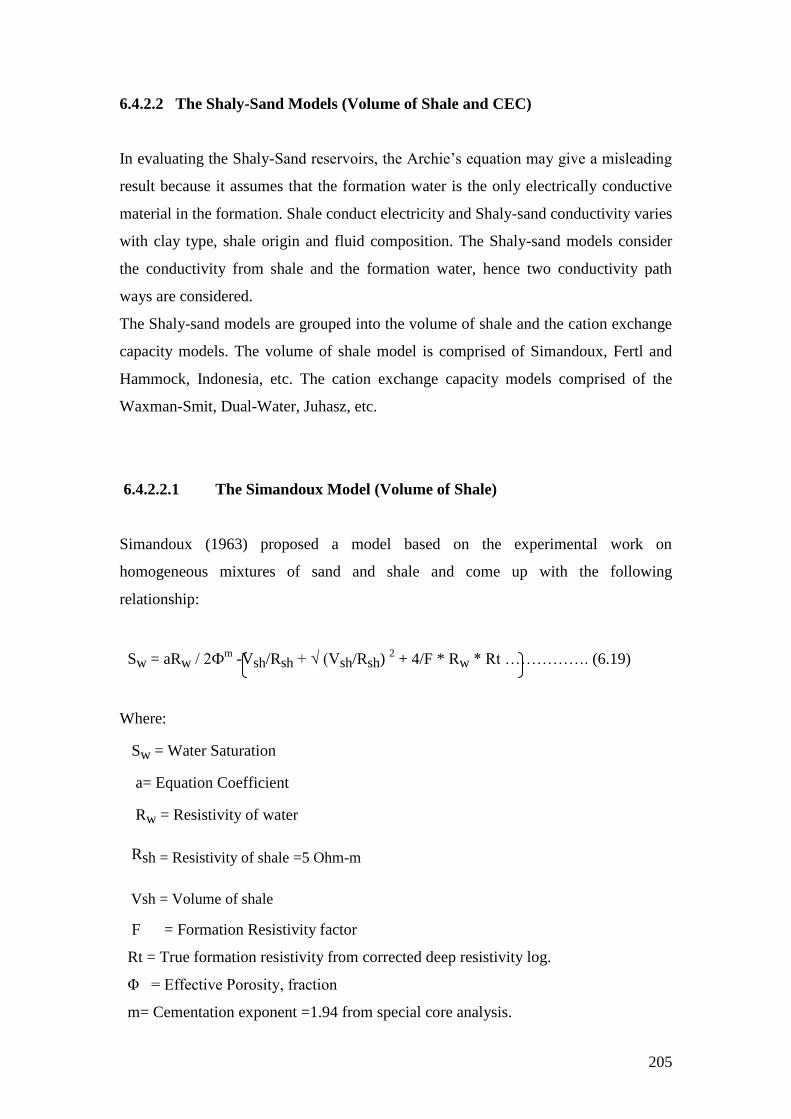
205

6.4.2.2 The Shaly-Sand Models (Volume of Shale and CEC)

In evaluating the Shaly-Sand reservoirs, the Archie‟s equation may give a misleading

result because it assumes that the formation water is the only electrically conductive

material in the formation. Shale conduct electricity and Shaly-sand conductivity varies

with clay type, shale origin and fluid composition. The Shaly-sand models consider

the conductivity from shale and the formation water, hence two conductivity path

ways are considered.

The Shaly-sand models are grouped into the volume of shale and the cation exchange

capacity models. The volume of shale model is comprised of Simandoux, Fertl and

Hammock, Indonesia, etc. The cation exchange capacity models comprised of the

Waxman-Smit, Dual-Water, Juhasz, etc.

6.4.2.2.1 The Simandoux Model (Volume of Shale)

Simandoux (1963) proposed a model based on the experimental work on

homogeneous mixtures of sand and shale and come up with the following

relationship:

Sw = aRw / 2Фm

-Vsh/Rsh + √ (Vsh/Rsh) 2 + 4/F * Rw * Rt ……………. (6.19)

Where:

Sw = Water Saturation

a= Equation Coefficient

Rw = Resistivity of water

Rsh = Resistivity of shale =5 Ohm-m


F = Formation Resistivity factor

Rt = True formation resistivity from corrected deep resistivity log.

Φ = Effective Porosity, fraction

m= Cementation exponent =1.94 from special core analysis.

206

The estimated resistivity of shale of 5 Ohm-m was used for the evaluation. This value

was determined from the resistivity correlation of wells as shown in Figure 6.13a

below)

Figure 6.13a: Estimate of resistivity of shale (Rsh) from Wells.

6.4.2.2.2 Indonesian Model

In 1971, Poupon and Leveaux proposed an empirical model called Indonesia formula

(Poupon and Leveaux1971).The equation was based on characteristic of fresh waters

and high degrees of shaliness that were present in many oil reservoirs in Indonesia.

The empirical relationship can be written as follows:

OP1Scale : 1 : 150


1

DEPTH

(M)

Gamma-Ray

GR (GAPI)0. 200.

Sonic Porosity

ILDC (OHMM)0.2 2000.

Lithology

VCL (Dec)0. 1.

Clay

Matrix

3375

OP3Scale : 1 : 150

DEPTH (3225.95M - 3242.2M) 2010/05/26 13:25

1

DEPTH

(M)

Gamma-Ray

GRn (API)0. 150.

Resistivity

ILDE (ohm.m)0.2 2000.

Lithology

VCL (DEC)0. 1.

Clay

Matrix

3370

3230

3240

Rsh=5

Ohm-m

Rsh=5

Ohmm

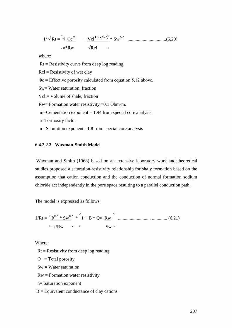
207

1/ √ Rt = √ Φem

+ Vcl (1-Vcl/2)

* Swn/2

..................................(6.20)

a*Rw √Rcl

where:

Rt = Resistivity curve from deep log reading

Rcl = Resistivity of wet clay

Φe = Effective porosity calculated from equation 5.12 above.

Sw= Water saturation, fraction

Vcl = Volume of shale, fraction

Rw= Formation water resistivity =0.1 Ohm-m.

m=Cementation exponent = 1.94 from special core analysis

a=Tortuosity factor

n= Saturation exponent =1.8 from special core analysis

6.4.2.2.3 Waxman-Smith Model

Waxman and Smith (1968) based on an extensive laboratory work and theoretical

studies proposed a saturation-resistivity relationship for shaly formation based on the

assumption that cation conduction and the conduction of normal formation sodium

chloride act independently in the pore space resulting to a parallel conduction path.

The model is expressed as follows:

1/Rt = Φm*

* Swn * 1 + B * Qv Rw ............................ ............. (6.21)

a*Rw Sw

Where:

Rt = Resistivity from deep log reading

Φ = Total porosity

Sw = Water saturation

Rw = Formation water resistivity

n= Saturation exponent

B = Equivalent conductance of clay cations

208

Qv = cation exchange capacity per pore volume (from equation 5.11)

m* = Cementation factor obtained from special core analysis measurement

determined from equation 5.6.

6.4.2.2.4 Dual-Water Model

The Dual-Water model is a modification of the Waxman-Smits equation by

considering counterion conductivity to be restricted to the bound water where

counterion resides and the free water which is found at a distance away from the clay

surface. The model shows that the apparent water conductivity will depend on the

relative volume of clay bound water and free water. Clavier et al. (1984) first

proposed this model called the dual water.

The Dual-Water equation is given below:

1/Rt = Φm*

* Swn * 1 + Swb 1 – 1 ..................................(6.22)

a Rw Sw Rwb Rw

Where:


Φ = Total porosity


Swb= Bound water saturation.


Rwb= Bound water resistivity


m* = Cementation factor obtained from special core analysis measurement.

Bound water is the water that is held close to the surface of the rock matrix. Bound

water is mainly associated with the surfaces of clay minerals because of their small

size .The saturation of bound water (Swb) determination is essential for an accurate

estimation of total water present in a reservoir. The presence of clay minerals and

mode of distribution in sandstone reservoirs often develop an overgrowth on the sand

grains that tends to provide additional pore spaces known as micro-pores that contain

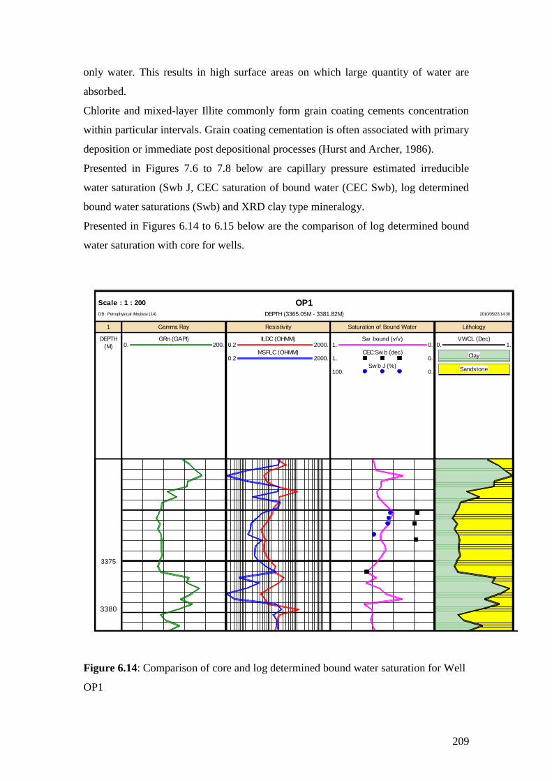
209

only water. This results in high surface areas on which large quantity of water are

absorbed.

Chlorite and mixed-layer Illite commonly form grain coating cements concentration

within particular intervals. Grain coating cementation is often associated with primary

deposition or immediate post depositional processes (Hurst and Archer, 1986).

Presented in Figures 7.6 to 7.8 below are capillary pressure estimated irreducible

water saturation (Swb J, CEC saturation of bound water (CEC Swb), log determined

bound water saturations (Swb) and XRD clay type mineralogy.

Presented in Figures 6.14 to 6.15 below are the comparison of log determined bound

water saturation with core for wells.

Figure 6.14: Comparison of core and log determined bound water saturation for Well

OP1

OP1Scale : 1 : 200


1

DEPTH

(M)

Gamma Ray

GRn (GAPI)0. 200.

Resistivity



Saturation of Bound Water

Sw bound (v/v)1. 0.

CEC:Sw b (dec)1. 0.

Sw b J (%)100. 0.

Lithology

VWCL (Dec)0. 1.

Clay

Sandstone

3375

3380

210

In well OP1 (Figure 6.14 above), 100 % bound water saturation was recorded at the

clay intervals top and below the reservoir zone. The core and log data overlaid do not

match and there was no XRD clay type result for this well. The minimum saturation

of bound water of about 62 % was recorded at measured depth 3272m.

In well OP2 (Figure 6.15), there exists a good agreement between the log and CEC

derived saturation of bound water. Within the reservoir interval, very low (less than

10 %) saturation of bound water was recorded and the dominant clay mineral present

is chlorite (track 5). The low resistivity values observed in track 3 may be due to the

presence of chlorite and illite.

OP2Scale : 1 : 250


1

DEPTH

(M)

GammaRay

GRn (GAPI)0. 200.

Resistivity

AT10 (OHMM)0.2 2000.

AT90 (OHMM)0.2 2000.

Saturation of Bound w ater

SWB1 (Dec)1. 0.

Sw b J (%)100. 0.

CEC:Sw b (dec)1. 0.

Lithology

VWCL (Dec)0. 1.

Sandstone

3450

3360

Figure 6.15: Comparison of core and log estimated bound water saturation and XRD

mineralogy data for Well OP2

211

6.4.2.2.5 Juhasz Model

Juhasz (1981) developed a relationship for determination of water saturation based on

the concept of Waxman and smith ( 1968).

1/Rt = Φm

* Swn * 1 + Bn * Qvn Rw ............................(6.23)

a*Rw Sw

Given that Qvn = Vcl * Φclay

Φ

Where:


Φ = Total porosity

Φclay = Total porosity of adjacent clay




Bn = Normalized equivalent conductance of clay cations

Qvn = Normalized cation exchange capacity per pore volume

m = Cementation factor

Vcl = Volume of clay, fraction.

6.4.3 Comparison of Conventional Core, Capillary Pressure and Log Water

Saturation

Water saturations were estimated from Dean-Stark conventional core based

measurements in well OP1 and OP3, and capillary pressure measurements in both

wells (chapter 5) which provide a reference against which log derived saturations can

be compared. Presented in Figures 6.16 to 6.17 below are the comparisons of

conventional core and capillary pressure water saturation measurements with log

calculated water saturation models.

212

Figure 6.16: Comparison of core and log water saturation models for Well OP1

OP1Scale : 1 : 150


1

DEPTH

(M)

GammaRay

GRn (GAPI)0. 200.

Resistivity



Archie' Model

Sw TArchT (Dec)1. 0.

Core Sw w ()100. 0.

Sw J (%)100. 0.

Vsh Models

Sw Sim (Dec)1. 0.

Sw ModSim (Dec)1. 0.

Sw Indo (Dec)1. 0.

Core Sw w ()100. 0.

Sw J (%)100. 0.

CEC Models

Sw TWS (Dec)1. 0.

Sw TDW (Dec)1. 0.

Sw TJuh (Dec)1. 0.

Sw TModSim (Dec)100. 0.

Sw TInd (Dec)100. 0.

Sw TJuh (Dec)100. 0.

Sw TWS (Dec)100. 0.

Core Sw w ()100. 0.

Sw J (%)100. 0.

Porosity/BVW

PHIT (Dec)0.5 0.

BVWSXO (Dec)0.5 0.

BVW (Dec)0.5 0.

Water

Lithology

VCLGR (Dec)0. 1.

Clay

Porosity

Sandstone

3375

Archie’s

Model

3370

213

The water saturation model derived from the Archie‟s model is plotted in track 4 (red

colour), shaly sand volume of shale models (Simandoux (Swsm- navy blue colour,

modified Simandoux (Swmodsim-red, and Indonesia (Sw Ind-green) in track 5; and

the CEC models (Waxman-Smit (Sw WS(navy blue, Dual water (Sw DW-red), and

Juhasz (Sw Juh –lime colour) in track 6 respectively.

In well OP1 (Figure 6.16) above, the average water saturation estimated from the

Archie‟s model was about 48%, Simandoux 67 %; Indonesia 84 %; Waxman-Smith

44 %,Dual –Water and Juhasz about 50 % respectively within the reservoir section.

The Waxman-Smith model in track 6 (navy blue colour) best matches with the water

saturation from routine core analysis and J-function saturation data.

214

Figure 6.17: Comparison of core and log water saturation models for Well OP3

OP3Scale : 1 : 250


1

DEPTH

(M)

GammaRay

GR (gAPI)0. 200.

Resistivity

ILDE (ohm.m)0.2 2000.


Archie Model

Sw ArchiT (Dec)1. 0.

CoreSw w ()100. 0.

Sw J (%)100. 0.

Vsh Models

Sw Simandoux (Dec)1. 0.

Sw ModSimandoux (Dec)1. 0.

Sw Indo (Dec)1. 0.

CoreSw w ()100. 0.

Sw J (%)100. 0.

CEC Models

Sw WS (Dec)1. 0.

Sw DW (Dec)1. 0.

Sw Juh (Dec)1. 0.

CoreSw w ()100. 0.

Sw J (%)100. 0.

Porosity/BVW

PHIT (Dec)0.5 0.

BVWSXO (Dec)0.5 0.

BVW (DEC)0.5 0.

Water

Lithology

VCLGR (Dec)0. 1.

Clay

Sandstone

OP3Scale : 1 : 250


3230

3240

3285

3275

215

For well OP3 (Figure 6.17) above, the estimated water saturation from Archie‟s

model was 44 % and 49 % ,Simandoux and Indonesia 40 % and 51 %, Waxman-

Smith, Dual-water and Juhasz 62 % and 48 % in both cored intervals respectively. A

good agreement between the capillary pressure water saturation and log determined

water saturation was observed in core 2 interval. The Simandoux and Indonesia

saturation models best match with the capillary pressure water saturation data.

Generally, the core based water based saturations are higher than those derived from

log. The higher water saturations in the core based saturations may be due to the water

based mud used to drill these wells which provide an alternate source for water found

in the core. Consistent mismatch in water saturation levels between log and core was

observed in all Well. It was apparent that from the logs and core data interpreted that

the reservoir formations contained shaly sands. The log interpretation compared water

saturation predictions from the clean sand (Archie) and Shaly Sand (Volume of shale

(Vsh) and Cation Exchange Capacity (CEC)) models. The Dual -Water and the

Simandoux models were the closest match with the core data.

6.5 BULK VOLUME OF WATER (BVW)

The bulk volume of water is defined as the product of water saturation and porosity.

The bulk volume of water can also be used as a hydrocarbon indicator (Walid, 2005).

This method simply plots a bulk volume of water (BVW) and effective porosity

versus reservoir depth interval. At points when the bulk volume of water is nearly or

equal to the effective porosity indicates that the zone or interval is wet or completely

saturated with water.

A separation between the bulk volume of water and effective porosity indicates the

presence of hydrocarbon. Presented in Figure 6.19 below is an example of the use of

bulk volume of water as hydrocarbon indicator for well OP3.

216

Figure 6.18: Bulk volume of water and effective porosity plot for well OP3

In conclusion, the Simandoux volume of shale water saturation model will be adopted

for water saturation calculations because there was an agreement with the

conventional core data and the water saturation derived from the capillary pressure

measurements. The input parameters into the Simandoux model can be controlled

much easier than the Dual-Water model.

Well OP3

Bulk Volume of water and Effective Porosity Plot

0.0001 0.06008 0.12006 0.18004 0.24002 0.3

PHIE and BVW

3240.

3237.8

3235.6

3233.4

3231.2

3229.

Me

as

ure

d D

ep

th (

m)

Bulk Volume of Water

Effective Porosity

Hydrocarbon

zone

Wet (100 % water saturation zone)

217

CHAPTER SEVEN

PERMEABILITY, ROCK TYPING AND FLOW UNITS

7.1 INTRODUCTION

Permeability is the property of a rock that characterises the flow of fluids through its

interconnected pores. It is a measure of the fluid conductivity of a rock. The

permeability of a flow unit in a reservoir is not an absolute value but it is a relative

value that varies with water saturation. Understanding how permeability is measured

is important to determine reservoir rock quality or compare the quality of one flow

unit to another. Permeability is not actually measured but is calculated and could be

determined horizontally or vertically.

The horizontal permeability is measured parallel to the bedding plane and is generally

greater than vertical because of vertical changes in sorting and because grains tends to

align and overlap parallel to the depositional surface. The vertical permeability is

measured across the bedding plane. Most permeability calculations are made from

horizontal measurements (Halliburton, 2001).

Reservoir contains water, oil and gas in varying amounts. Each of the fluid present in

the reservoir interferes with and impedes the flow of other fluid. The permeability of a

reservoir calculated with only one fluid present in the pores of a formation is regarded

as absolute (Ka). Effective permeability (Ke) is the ability of a rock to conduct one

fluid in the presence of another, provided that both fluids are immiscible. Relative

permeability (Kr) can be expressed as the ratio of a fluid‟s effective permeability to

the formation‟s absolute permeability. It can be expressed as a number between zero

and one or as a percent.

The calibration of test data made at in situ reservoir conditions with laboratory

measurements is very important in reservoir description. In situ permeability is a

measure of effective permeability of a given fluid in the presence of other fluids.

Permeability measured under laboratory conditions is the absolute permeability to a

single fluid (Hurst & Archer, 1986).

A petrophysical flow unit is defined as an interval of sediment with similar

petrophysical properties such as porosity, permeability, water saturation, pore throat

radius and flow capacity that are different from the intervals immediately above and

below it (Porras & Campos, 2001).Petrophysical flow units are grouped to define

49 bbl

/day of

Water

reported

On DST

Test

result.

218

containers and rock types having similar flow capacity are grouped and used to

determine reservoir flow units.

Ebanks (1987) defined the fundamental concept of hydraulic flow units as a map- able

portion of the reservoir within which geological and petrophysical properties

controlling the flow of fluids, are consistent and predictably different from the

properties of other reservoir rock portion. Methods for flow unit zonation include

application of Lorenz plots and the use of flow zone indicator (Saibal et al., 2008).

Both methods require the knowledge of porosity and permeability distributions.

Different techniques and methods have been used to define flow units. Comparative

studies of different methods of flow unit determination have been reported by Porras

et al. (1999), Amaefule et al. (1993) and Stolz & Graves (2003).

Rock typing is the process of classifying reservoir rocks into distinct units, each of

which was deposited under similar geological conditions and has undergone similar

diagenetic alterations (Gunter et al., 1997).When properly applied, rock typing can

lead to an accurate estimation of formation permeability in uncored intervals of

uncored well (Genliang et al., 2007).

The flow rate depends on the permeability, formation pressure, and viscosity of the

fluid and saturation of the fluids present.

7.2 PERMEABILITY

The permeability values in this study are derived from three potential sources. They

are core measured permeabilities, permeability estimated from the regression analysis

of the core porosity versus permeability plot; log predicted permeabilities and

permeability determined from the repeat formation test measurements.

7.2.1 Permeability from Core Analysis (Permeability–Porosity Function)

This particular aspect of the study was aimed at establishing a correlation between

core permeability and porosity and other wireline log porosity responses. The

objective was to identify or predict permeability in uncored intervals and also to

estimate permeability in wells without core data. The Figure 7.1 below present the

graphics of core analysis porosity-permeability plots for well OP1, OP2, OP3, and

combination of all the wells.

219

Figure 7.1: Porosity –Permeability cross plots for determination of function

The following based permeability-porosity functions were established from the cross

plots as discussed in chapter four of this study as shown in Table 7.1 below

Table 7.1: Established porosity-permeability functions for wells

Well Porosity-Permeability functions Correlation Coefficient (R2)

OP1 Log (K) = -3.1626 +24.817 * Porosity 0.8931

OP2 Log (K)= -2.687 +21.6648 * Porosity 0.9379

OP3 Log (K)= -1.8403 + 16.9376 * Porosity 0.9141

All Well Log (K)= -2.4284 + 20.8917 * Porosity 0.9201

LogK(air) =-3.0412+25.6441*Phic

R2=0.89

Well OP1

Porosity-Permeability Plot

0. 0.06 0.12 0.18 0.24 0.3

Core Porosity (v/v)

0.001

0.01

0.1

1.

10.

100.

1000.

A6

A5

A4

A3

A2

A1

0.

6.

Facies


R2= 0.8931

A4

Facies

A6

Well OP2


0. 0.06 0.12 0.18 0.24 0.3Core Porosity (v/v)

0.001

0.01

0.1

1.

10.

100.

1000.

A6

A5

A4

A3

A2

A1

0.

6.Facies


R2= 0.9379

Facies

A6 & A5

A1,A2 &

A3

A4

Well OP3


0. 0.06 0.12 0.18 0.24 0.3Core Porosity (v/v)

0.001

0.01

0.1

1.

10.

100.

1000.

A6

A5

A4

A3

A2

A1

0.

6.Facies


R2= 0.9141

Facies

A6

Facies

A3 & A4

All Well


0. 0.06 0.12 0.18 0.24 0.3

Core Porosity (v/v)

0.001

0.01

0.1

1.

10.

100.

1000.

10000.

A6

A5

A4

A3

A2

A1

0.

6.Facies


R2= 0.9201

Well

OP1

OP2

OP3

A5 & A6

A1 &A2

A3 & A4

Pe

rme

ab

ility

(m

D)

Pe

rme

ab

ility

(m

D)

Pe

rme

ab

ility

(m

D)

Pe

rme

ab

ility

(m

D)

220

The functions established in Table 7.1 above have been validated by comparing

predicted permeabilities from the functions against the original core measured

permeabilities. The comparison of the functions are illustrated in Figures 7.2 to 7.4

below where the predicted permeabilities (red colour curve in track 4) are directly

overlain with the core permeabilities (green colour dots in track 4) in wells OP1, OP2

and OP3 respectively.

Figure 7.2: Well OP1 plot of predicted permeability overlaying original core

permeability in track 4

In well OP1 (Figure 7.2), the predicted permeability (track4 red) values from log

derived porosity matched very well with the core measured permeability (track 4

green dots). A good relationship was observed between both curves though they both

portray the same trend pattern. The plot for well OP2 is presented in Figure 7.3 below.

OP1Scale : 1 : 150


1

DEPTH

(M)

Gamma-Ray

GR (GAPI)0. 200.

Resistivity



Permeability

Predicted K (mD)0.001 1000.


Lithology

VCL (Dec)0. 1.

Clay

Matrix

3375

3380

3370

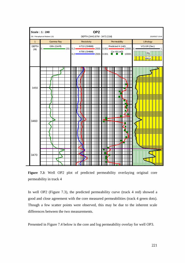
221



In well OP2 (Figure 7.3), the predicted permeability curve (track 4 red) showed a

good and close agreement with the core measured permeabilities (track 4 green dots).

Though a few scatter points were observed, this may be due to the inherent scale

differences between the two measurements.

Presented in Figure 7.4 below is the core and log permeability overlay for well OP3.

OP2Scale : 1 : 240


1

DEPTH

(M)

Gamma-Ray

GRn (GAPI)0. 150.

Resistivity

AT10 (OHMM)0.2 2000.

AT90 (OHMM)0.2 2000.

Permeability


Cor Kli (mD)0.001 10000.

Lithology

VCLGR (Dec)0. 1.

Clay

Matrix

3450

3460

3470

222



For well OP3 (Figure 7.4), the predicted permeability matched the core permeability

on a one to one trend in core 1(measured depth interval between 3230m to 3240m).In

OP3Scale : 1 : 250


1

DEPTH

(M)

GammaRay

GR (gAPI)0. 200.

Resistivity

ILDE (ohm.m)0.2 2000.


Permeability


Cor Klin ()0.001 1000.

Lithology

VCLGR (Dec)0. 1.

Clay

Sandstone

OP3Scale : 1 : 250


3230

3240

3280

3285

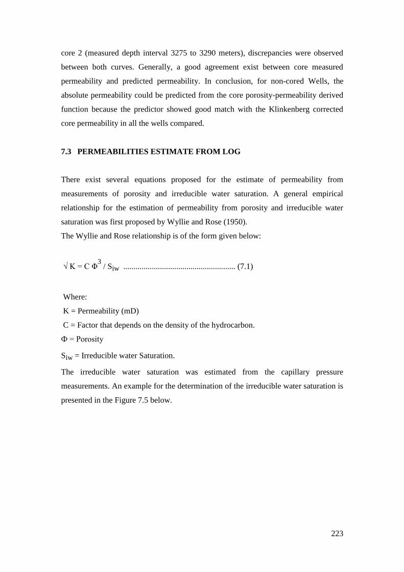
223

core 2 (measured depth interval 3275 to 3290 meters), discrepancies were observed

between both curves. Generally, a good agreement exist between core measured

permeability and predicted permeability. In conclusion, for non-cored Wells, the

absolute permeability could be predicted from the core porosity-permeability derived

function because the predictor showed good match with the Klinkenberg corrected

core permeability in all the wells compared.

7.3 PERMEABILITIES ESTIMATE FROM LOG

There exist several equations proposed for the estimate of permeability from

measurements of porosity and irreducible water saturation. A general empirical

relationship for the estimation of permeability from porosity and irreducible water

saturation was first proposed by Wyllie and Rose (1950).

The Wyllie and Rose relationship is of the form given below:

√ K = C Φ3 / Siw ....................................................... (7.1)

Where:


C = Factor that depends on the density of the hydrocarbon.

Ф = Porosity

Siw = Irreducible water Saturation.

The irreducible water saturation was estimated from the capillary pressure

measurements. An example for the determination of the irreducible water saturation is

presented in the Figure 7.5 below.

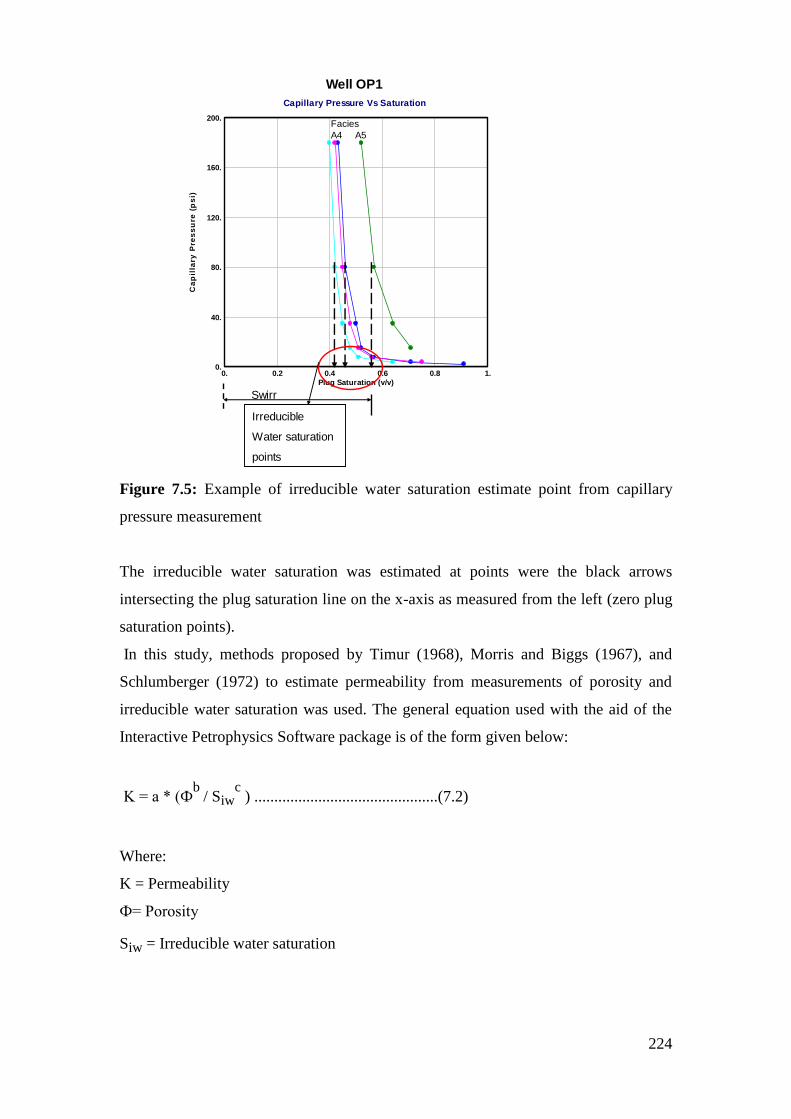
224

Figure 7.5: Example of irreducible water saturation estimate point from capillary

pressure measurement

The irreducible water saturation was estimated at points were the black arrows

intersecting the plug saturation line on the x-axis as measured from the left (zero plug

saturation points).

In this study, methods proposed by Timur (1968), Morris and Biggs (1967), and

Schlumberger (1972) to estimate permeability from measurements of porosity and

irreducible water saturation was used. The general equation used with the aid of the

Interactive Petrophysics Software package is of the form given below:

K = a * (Фb

/ Siwc ) ..............................................(7.2)

Where:

K = Permeability

Ф= Porosity

Siw = Irreducible water saturation

Well OP1


0. 0.2 0.4 0.6 0.8 1.


0.

40.

80.

120.

160.

200.

Ca

pil

lary

Pre

ss

ure

(p

si)

A5A4

Facies

Irreducible

Water saturation

points

Swirr

225

The constants a, b and c for Timur, Morris and Biggs, and Schlumberger equations are

given below:

Timur equation= a = 8581; b = 4.4 and c = 2

Morris Biggs gas = a= 62500; b = 6 and c = 2

Schlumberger =a = 10000; b = 4.5 and c = 2

Comparison of log permeability values are presented in Figures 7.4 to 7.6. The Morris

and Biggs equation is plotted in track 3(red colour curve), Schlumberger in track 4

(blue colour curve), and the Timur equation in track 5 (Pink colour curve). The curves

were overlaid with the core measured permeability data (green colour dots) in tracks 3

to 5 for comparison.

226

Figure 7.6: Log estimated permeability and overlaid core permeability for well OP1

OP1Scale : 1 : 100


1

DEPTH

(M)

GammaRay

GRn (GAPI)0. 200.

MORRIS BIG PERM

Morris Biggs P (md)0.01 100.


SCHLUMBERGER PERM

Schlumberger P (md)0.01 100.

Core Kair (mD)0.01 100.

TIMUR PERM

Timur Permeab (md)0.01 100.


Lithology

VWCL (Dec)0. 1.

Clay

Sandstone

3375

3370

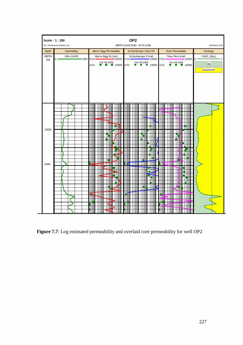
227

OP2Scale : 1 : 250


Depth

DEPTH

(M)

GammaRay

GRn (GAPI)0. 200.

Morris Bigg Permeability

Morris Bigg Pe (md)0.01 10000.

Cor Kli (mD)0.01 10000.

Schlumberger Chart K3


Cor Kli (mD)0.01 10000.

Timur Permeability

Timur Perm (md)0.01 10000.

Cor Kli (mD)0.01 10000.

Lithology

VWCL (Dec)0. 1.

Clay

Sandstone

3450

3460


228

OP3Scale : 1 : 200


1

DEPTH

(M)

GammaRay

GrC (GAPI)0. 150.

Morris Biggs Gas

Morrisgas1 (md)0.001 1000.

Cor Klin ()0.001 1000.

Schlumberger Chart K3


Cor Klin ()0.001 1000.

Timur Permeability

Timur Permeabi (md)0.001 1000.

Cor Klin ()0.001 1000.

Lithology

VWCL (Dec)0. 1.

Clay

Sandstone

OP3Scale : 1 : 200


3240

3230

3280

3290


The Morris and Biggs equation best match with the core measured permeability

followed by the Timur equation in all well. The reason of for this investigation was to

estimate in situ permeability using capillary pressure irreducible water saturation and

log porosity with the models proposed by Timur, Morris Biggs for gas, and

Schlumberger to determine which model best agree with the core permeability

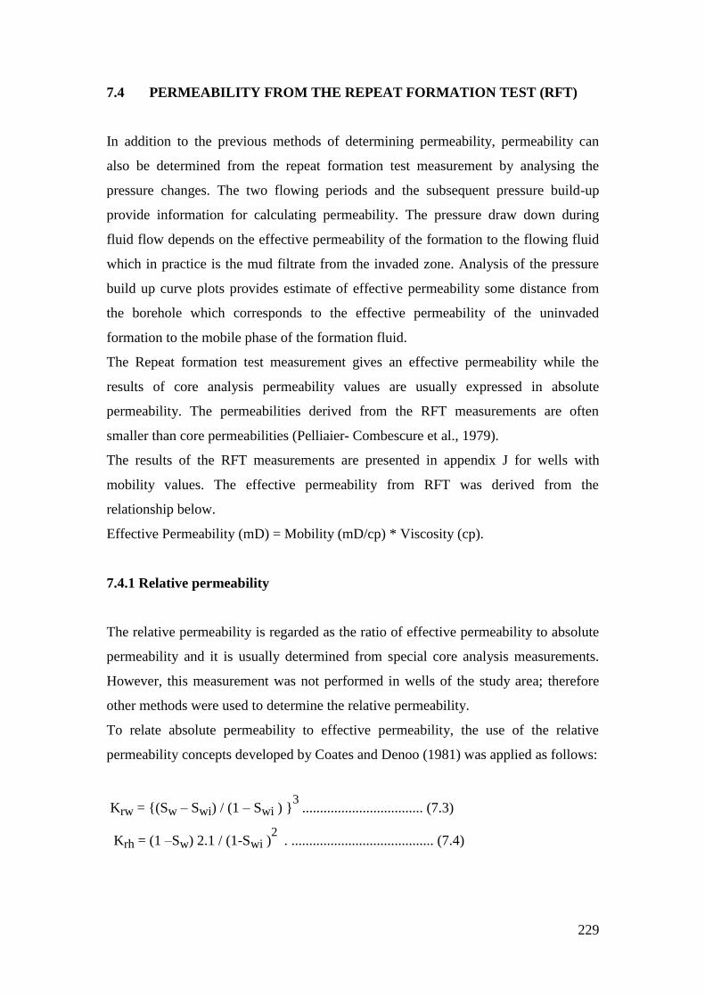
229

7.4 PERMEABILITY FROM THE REPEAT FORMATION TEST (RFT)

In addition to the previous methods of determining permeability, permeability can

also be determined from the repeat formation test measurement by analysing the

pressure changes. The two flowing periods and the subsequent pressure build-up

provide information for calculating permeability. The pressure draw down during

fluid flow depends on the effective permeability of the formation to the flowing fluid

which in practice is the mud filtrate from the invaded zone. Analysis of the pressure

build up curve plots provides estimate of effective permeability some distance from

the borehole which corresponds to the effective permeability of the uninvaded

formation to the mobile phase of the formation fluid.

The Repeat formation test measurement gives an effective permeability while the

results of core analysis permeability values are usually expressed in absolute

permeability. The permeabilities derived from the RFT measurements are often

smaller than core permeabilities (Pelliaier- Combescure et al., 1979).

The results of the RFT measurements are presented in appendix J for wells with

mobility values. The effective permeability from RFT was derived from the

relationship below.

Effective Permeability (mD) = Mobility (mD/cp) * Viscosity (cp).

7.4.1 Relative permeability

The relative permeability is regarded as the ratio of effective permeability to absolute

permeability and it is usually determined from special core analysis measurements.

However, this measurement was not performed in wells of the study area; therefore

other methods were used to determine the relative permeability.

To relate absolute permeability to effective permeability, the use of the relative

permeability concepts developed by Coates and Denoo (1981) was applied as follows:

Krw = {(Sw – Swi) / (1 – Swi ) }3

.................................. (7.3)

Krh = (1 –Sw) 2.1 / (1-Swi )2

. ........................................ (7.4)

230

Where:

Krw = Water Relative permeability


Swi = Irreducible water saturation

Krh = Hydrocarbon relative permeability.

The results of the application of equations 7.3 and 7.4 above to wells OP2 and OP3

are presented in Figure 7.9 below.

Well OP3

Rekative Permeability Vs Water Saturation Plot for Core 1

0. 0.2 0.4 0.6 0.8 1.

Water Saturation (v/v)

0.

0.2

0.4

0.6

0.8

1.R

ela

tiv

e p

erm

ea

bil

ity

Kr

Well OP2

Estimated Relative Permeability Vs Water Saturation

0. 0.2 0.4 0.6 0.8 1.


0.

0.2

0.4

0.6

0.8

1.

Re

lati

ve

Pe

rme

ab

ilit

y K

r

Krh

Krw

Krh=Krw

Irreducible water

saturation

Irreducible

water saturation

Krh=Krw

Krh

Krw

Irreducible

hydrocarbon

saturation Sxo

Figure 7.9: Relative permeability curves for well OP2 and OP3 within the reservoir

intervals

According to Timmerman (1982), clays usually have poor relative permeability

characteristics and higher or in-situ irreducible water saturation. Considering the

relative permeability curves of Figure 7.9 above of well OP2 and OP3, it was

observed that the irreducible water saturation of well OP2 is approximately 17 % and

Well OP3 is approximately 30 %. From this result, it can be inferred that well OP2

has better rock quality as compared to well OP3 in terms of irreducible water

saturation.

At the intersection of Krh and Krw curves, hydrocarbon and water flow at ease.

231

The comparison of permeabilities derived from core, log, RFT, and relative

permeability equation for well OP2 is presented in Figure 7.10 below.

OP2Scale : 1 : 250


Depth

DEPTH

(M)

GammaRay

GRn (GAPI)0. 200.

Comparison of Permeability(Log,RFT,Estimated)

Moriis Biggs G (md)0.001 10000.

RFT K ()0.001 10000.

K from Krh ()0.001 10000.

Comparison of Effective Permeability

Timur Perm (md)0.001 10000.

RFT K ()0.001 10000.

K from Krh ()0.001 10000.

Comparison of Effective Permeability

Schlumberger (md)0.001 10000.

RFT K ()0.001 10000.

K from Krh ()0.001 10000.

Lithology

VWCL (Dec)0. 1.

Clay

Sandstone

3450

3460

Figure 7.10: Comparison of permeabilities derived from log, RFT and Krh equations

for well OP2

Tracks 3, 4 and 5 of Figure 7.10 above are the log estimated permeability curves

overlain with RFT determined effective permeability(brown dots), and effective

permeability estimated from the product of Krh with core permeability (K from Krh,

black dots).

232

The Morris Biggs log estimated permeability (track 3) best agree with the effective

permeability derived from the RFT measurement.

In conclusion, it has been demonstrated that permeability derived from the repeat

formation test (RFT) measurements are effective permeabilities and showed good

agreement with log derived permeability using the Morris Biggs gas model. The

predicted permeability from convention core porosity-permeability data best agree

with the Klinkenberg corrected permeability as presented in track 4 of Figure 7.11

below.

Figure 7.11: Comparison of permeabilities derived from core, log and cross plot

OP2Scale : 1 : 200


1

DEPTH

(M)

Gamma-Ray

GRn (GAPI)0. 200.

Caliper

HCA6.16.

Comparison Of Permeabilities


Moriis Biggs G (md)0.001 10000.

Core Klinkenb ()0.001 10000.

RFT (K) ()0.001 10000.

Resistivity

AT90 (OHMM)0.2 2000.

AT10 (OHMM)0.2 2000.

3450

3460

3470

233

7.5 DETERMINATION OF ROCK TYPES (PETROFACIES)

The petrofacies concept is used for the study of rock units according to their

petrologic characteristics as opposed to their form, boundaries or in relation to other

rock units. The quality of reservoirs is controlled by depositional structures, textures

and composition, diagenetic processes and pore types distribution. The term

petrofacies is defined in the sedimentary literature by different meanings (De Ros &

Goldberg, 2007). Petrofacies analysis in this part of the study is applied based on flow

units that relates pore types, porosity and permeability as an assessment of reservoir

continuity and quality.

Petrofacies are defined as intervals of rocks with a similar average in pore throat

radius having similar fluid flow characteristics. The characterization of the rock type

is based on the flow capacity and storage of the rock carried out from capillary results,

porosity and permeability values (Boada et al., 2001).

Pore throat size may be estimated from routine core analysis porosity and

permeability data at ambient conditions. Rock type characterization can be based on

integration of routine core analysis data, capillary pressure data, thin section, scanning

electron microscopy, and X-Ray diffraction analysis in core samples to determine

dominant pore throat radius of the interconnected pore system. Two methods

commonly used to assess reservoir quality on the basis of pore throat are the Winland

method and Pittman‟s methods are used in this study.

Winland (1972) of Amoco tested 322 different water wet rocks using mercury

injection capillary pressure curves to develop an empirical relationship between

porosity, permeability and pore throat radius on reservoir rocks from Spindle field,

Colorada. Winland‟s experiments showed that the effective pore system that

dominates flow through a rock corresponds to a mercury saturation at 35 %.That pore

system has pore throat radii equal to or smaller than the pore throats entered when a

rock is saturated 35% with a non-wetting phase. After 35 % of the pore system fills

with a non-wetting fluid, the remaining pore system does not contribute to flow;

instead it contributes to storage (Winland, 1972).

The r35 pore throat radii is a function of entry size and pore throat sorting, and is a

good measure of the largest connected pore throats in a rock with intergranular

porosity (Hartmann & Coalson, 1990). The Winland equation was used and published

by Kolodzie in 1980 and the equation is given as below:

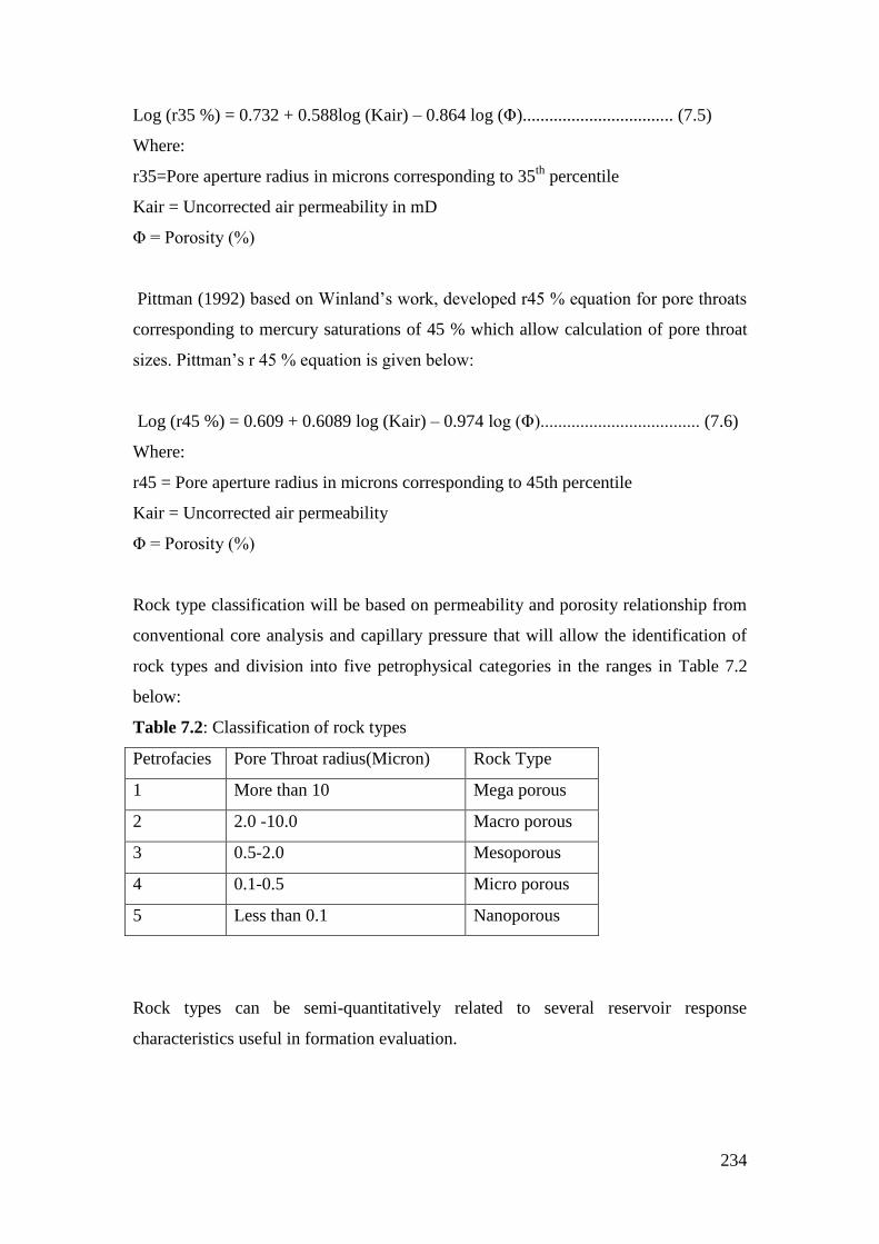
234

Log (r35 %) = 0.732 + 0.588log (Kair) – 0.864 log (Φ).................................. (7.5)

Where:

r35=Pore aperture radius in microns corresponding to 35th

percentile

Kair = Uncorrected air permeability in mD

Φ = Porosity (%)

Pittman (1992) based on Winland‟s work, developed r45 % equation for pore throats

corresponding to mercury saturations of 45 % which allow calculation of pore throat

sizes. Pittman‟s r 45 % equation is given below:

Log (r45 %) = 0.609 + 0.6089 log (Kair) – 0.974 log (Φ).................................... (7.6)

Where:

r45 = Pore aperture radius in microns corresponding to 45th percentile

Kair = Uncorrected air permeability

Φ = Porosity (%)

Rock type classification will be based on permeability and porosity relationship from

conventional core analysis and capillary pressure that will allow the identification of

rock types and division into five petrophysical categories in the ranges in Table 7.2

below:

Table 7.2: Classification of rock types

Petrofacies Pore Throat radius(Micron) Rock Type

1 More than 10 Mega porous

2 2.0 -10.0 Macro porous

3 0.5-2.0 Mesoporous

4 0.1-0.5 Micro porous

5 Less than 0.1 Nanoporous

Rock types can be semi-quantitatively related to several reservoir response

characteristics useful in formation evaluation.

235

7.5.1 Well OP1 Petrofacies determination

To determine the dominant pore throat radius that best reproduce capillary pressure

data, permeability and porosity of the well, the Winland and Pittman‟s equations (7.5

and 7.6) are used and the results are shown in Table 7.3 below.

Table 7.3: Rock types classification based on winland and Pittman calculations

Depth (m)

Porosity (%)

Kair

(mD)

Winland (r35) (Microns)

Pittman (r45) (Microns)

Rock Type (Petrofacies)

3370.05 18.9 108 6.6 4.10 2=Macro

3370.6 20.2 64 4.6 2.69 2=Macro

3371.07 16.9 40 4.1 2.45 2=Macro

3371.4 16.4 14 2.2 1.32 3=Meso

3371.9 16.5 26 3.3 1.95 2=Macro

3372.03 12.7 6.0 1.7 1.02 3=Meso

3372.53 9.5 0.32 0.4 0.23 4=Micro

3372.98 6.9 0.16 0.3 0.20 4=Micro

3373.75 5.0 0.018 0.03 0.07 5=Nanno

3375.6 3.0 0.017 0.2 0.12 4=Micro

3375.98 2.0 0.016 0.26 0.17 4=Micro

3376.62 7.7 0.03 0.1 0.06 5=Nanno

3376.86 8.6 0.151 0.26 0.16 4=Micro

3377.12 10.1 0.33 0.38 0.22 3=Meso

3377.36 9.6 0.151 0.25 0.14 4=Micro

3377.54 7.0 0.079 0.22 0.13 4=Micro

3377.78 7.9 0.104 0.24 0.14 4=Micro

3378.23 9.2 0.028 0.09 0.05 5=Nano

3378.48 8.6 0.025 0.09 0.05 5=Nano

3378.58 7.6 0.025 0.1 0.06 5=Nano

3379.24 6.8 0.018 0.09 0.05 5=Nano

3379.64 1.2 0.013 0.36 0.24 4=Micro

3379.82 4.9 0.01 1.4 0.05 3=Meso

3380.15 3.3 0.015 1.96 0.09 3=Meso

Table 7.3 above shows the calculated pore throat radii from Winland and Pittman

equations of the reservoir rock porosity, permeability and pore throat radii ranges by

rock type. Four possible petrophysical rock types were identified based on pore throat

radii and results will be validated with thin section analysis and Scanning electron

microscopy results. Petrofacies 2 represent the best reservoir rock type in this Well

characterised by a porosity range between 16 % and 20 % and an average

permeability of 59mD. The rock types in this depth interval (3370.40 to 3371.6m)

represents rocks having similar flow capacity and higher storage capacity than other

rocks. Petrofacies 5 is a non productive due to the inability of these rock types to

236

contribute to flow and not having storage capability. The porosity of these Petrofacies

5m ranges from 1.6 % to 9.2 % with an average permeability of approximately

0.1mD.

In order to determine whether the core plug data generally conform to Winland or

Pittman, a correlation was made with the permeability and the Pittman‟s equation

having a correlation coefficient of 90 % best fit with permeability values (Figure

7.12); therefore it was adopted for rock type classification.

Correlation of Winland and Pittman with

Permeability of well OP1

Pittman(y) = 4.9827x2.0712

R2 = 0.9089

Winland(y) = 0.841x1.6291

R2 = 0.6243

0.01

0.1

1

10

100

0.1 1.1 2.1 3.1 4.1 5.1 6.1 7.1

Pore Throat Radius (Microns)

Pe

rme

ab

ilit

y (

mD

)

Winland Pittman Power (Pittman) Power (Winland)

Figure 7.12: Correlation of Winland and Pittman‟s plots for well OP1


The reservoir rocks in well OP2 were classified based on pore throat radius (r35) of

Winland. The characterization was based on the flow capacity and storage carried out

237

from the routine core porosity and permeability values. Table 7.4 below presents the

results from the analysis and rock type classifications.

Table 7.4: Rock types classification based on winland and Pittman calculations for

well OP2

Depth (m)

Porosity (%)

Kair (mD)

Winland(r35) (Microns)

Pittman(r45) (Microns)

Petrofacies Rock Type

3446.20 23.06 392 11.8 7.3 Mega 1

3447.08 24.24 227 8.3 4.9 Macro 2

3447.11 24.17 166 7.1 4.1 Macro 2

3447.83 18.65 14.2 2 1.2 Meso 3

3448.69 22.01 30.3 2.8 1.6 Macro 2

3449.52 20.27 13.3 1.8 1 Meso 3

3450.58 22.32 165 7.4 4.4 Macro 2

3451.70 23.54 366 12.6 6.8 Mega 1

3452.14 23.83 606 14.8 9.2 Mega 1

3452.59 24.01 435 12.6 7.4 Mega 1

3453.68 23.03 296 10 6.1 Mega 1

3454.72 24.25 909 19 11.5 Mega 1

3455.08 22.96 1095 20.1 13.6 Mega 1

3455.55 18.83 28.1 3.1 1.8 Macro 2

3455.86 10.42 2.07 1.1 0.6 Meso 3

3456.15 4.59 .019 0.1 0.1 Nano 5

3456.65 3.37 .021 0.2 0.1 Micro 4

3457.18 3.27 .006 0.1 0.1 Meso 3

3457.74 21.39 225 9.1 5.6 Macro 2

3458.69 21.36 270 10 6.2 Mega 1

3459.59 20.11 213 9.3 5.7 Macro 2

3460.00 21.93 399 12.6 7.7 Mega 1

3460.10 22.05 675 17.4 10.5 Mega 1

3461.48 23.07 473 13.5 8.1 Mega 1

3462.54 18.91 33.1 3.3 1.9 Macro 2

3463.48 19.55 110 6.2 3.9 Macro 2

3464.59 8.19 .100 0.23 0.1 Micro 4

3464.81 4.92 .037 0.2 0.1 Micro 4

3465.40 2.95 .005 0.1 0.1 Nano 5

3466.47 6.23 .015 0.1 0.1 Nano 5

3466.75 4.43 .092 0.4 0.2 Micro 4

3467.50 4.12 .054 0.3 0.2 Micro 4

3467.60 3.89 .018 0.16 0.1 Nano 5

3468.17 5.96 .020 0.1 0.1 Nano 5

3468.89 7.23 .028 0.12 0.1 Nano 5

3470.30 6.80 3.07 2 1.2 Meso 3

A plot of pore throat radius calculated from the Winland and Pittman equations versus

the permeability for well OP2 is given in Figure 7.13 below. It was observed from the

regression correlation coefficient that the Winland equation best correlate with the

permeability values and hence was used to classify the reservoir rocks.

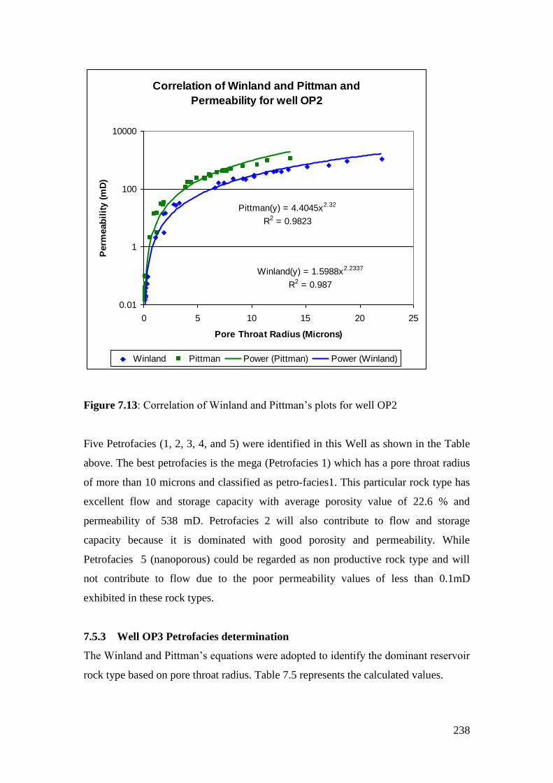
238

Correlation of Winland and Pittman and

Permeability for well OP2

Pittman(y) = 4.4045x2.32

R2 = 0.9823

Winland(y) = 1.5988x2.2337

R2 = 0.987

0.01

1

100

10000

0 5 10 15 20 25

Pore Throat Radius (Microns)

Perm

eab

ilit

y (

mD

)



Five Petrofacies (1, 2, 3, 4, and 5) were identified in this Well as shown in the Table

above. The best petrofacies is the mega (Petrofacies 1) which has a pore throat radius

of more than 10 microns and classified as petro-facies1. This particular rock type has

excellent flow and storage capacity with average porosity value of 22.6 % and

permeability of 538 mD. Petrofacies 2 will also contribute to flow and storage

capacity because it is dominated with good porosity and permeability. While

Petrofacies 5 (nanoporous) could be regarded as non productive rock type and will

not contribute to flow due to the poor permeability values of less than 0.1mD

exhibited in these rock types.


The Winland and Pittman‟s equations were adopted to identify the dominant reservoir

rock type based on pore throat radius. Table 7.5 represents the calculated values.

239

Table 7.5: Reservoir rock classifications of well OP3

Depth (m)

Porosity (%)

Kair (mD)

Winland(r35) (Microns)

Pittman(r45) (Microns)

Rock Type (Petrofacies)

Rock Type

3236.1 24.2 135 6.0 3.6 Macro 2

3236.35 22.6 156 7.0 4.2 Macro 2

3236.51 21.3 86 5.3 3.1 Macro 2

3236.81 21.4 77 4.8 2.9 Macro 2

3237.05 18.1 34 3.6 2.1 Macro 2

3237.26 18.1 43 4.1 2.4 Macro 2

3237.51 15.0 21 3.1 1.9 Macro 2

3237.77 12.9 8.6 2.1 1.2 Meso 3

3237.95 9.1 0.63 0.6 0.4 Meso 3

3238.3 8.9 0.22 0.33 0.2 Micro 4

3238.5 6.3 0.074 0.24 0.1 Micro 4

3238.52 8.8 0.23 0.34 0.2 Micro 4

3239.05 4.3 0.06 0.29 0.2 Micro 4

3243.6 0.6 0.04 1.26 0.9 Meso 3

3283.2 19.2 4.9 1.05 0.6 Meso 3

3283.6 17.8 15 2.2 1.3 Meso 3

3283.85 17.8 30 3.3 1.9 Macro 2

3284.1 20.4 41 3.6 2.1 Macro 2

3284.35 21.3 40 3.3 1.9 Macro 2

3284.45 22 62 4.7 2.5 Macro 2

3285.05 22.2 50 3.6 2.1 Macro 2

3285.3 22.8 47 3.5 2 Macro 2

3285.34 20.6 15 1.9 1.1 Meso 3

3285.83 17.3 4.8 1.2 0.7 Meso 3

3286.08 14.3 45 5.2 3.1 Macro 2

3286.3 20.4 53 3.9 2.4 macro 2

3286.55 22.3 48 3.6 2.1 Macro 2

3286.6 22.2 79 4.7 2.8 macro 2

3287.25 23.3 2.7 0.66 0.3 Meso 3

3287.3 15.8 77 6.2 3.9 macro 2

3287.9 3.7 0.194 0.66 0.4 Meso 3

3290.06 2.3 0.013 0.21 0.1 Micro 4

3291.76 2.7 0.016 0.18 0.1 Nano 5

Four rock types (2, 3, 4 and 5) were identified based on pore throat radius of Winland

and Pittman. Petrofacies 2 was identified as the best reservoir rock in this Well and

has a flow and storage capacity having porosity range of 23 % to 24 % and

permeability values from 57mD to 105mD. Petrofacies 3 (meso porous) is relatively

fair to poor rock type which may contribute to flow. Petrofacies 4 and 5 were

classified as non productive rock types because of the very low permeability values of

less than 0.1mD exhibited.

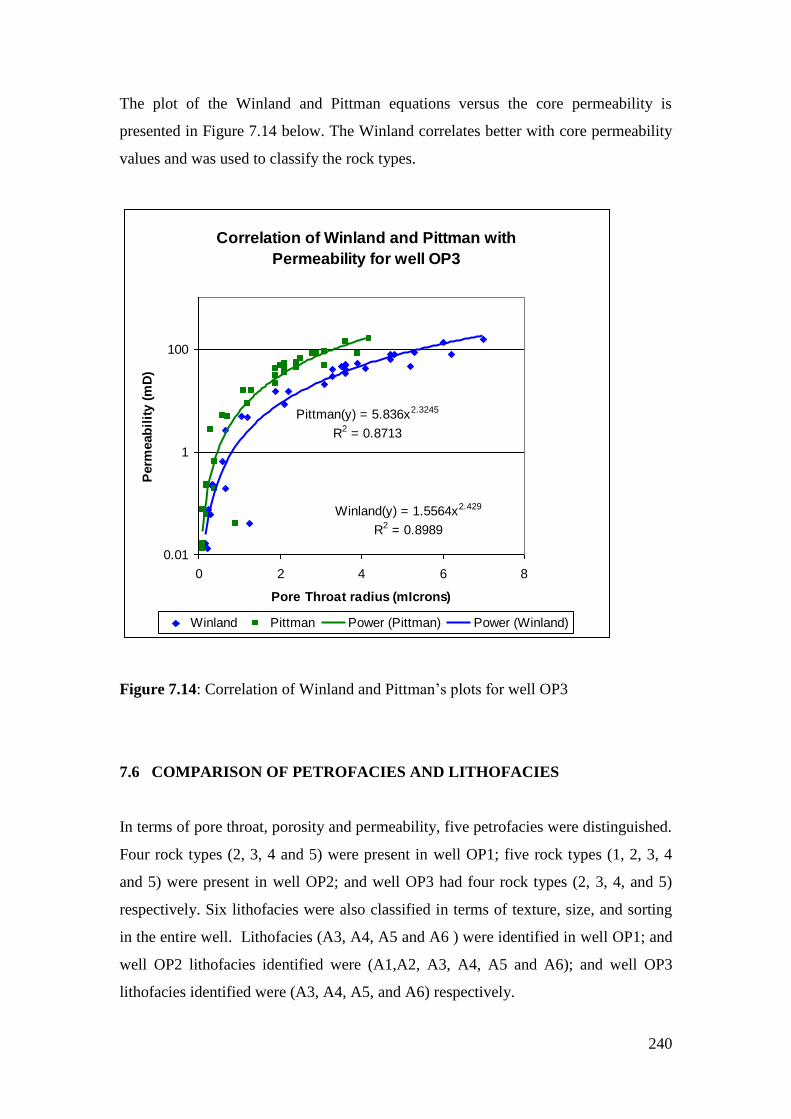
240

The plot of the Winland and Pittman equations versus the core permeability is

presented in Figure 7.14 below. The Winland correlates better with core permeability

values and was used to classify the rock types.

Correlation of Winland and Pittman with

Permeability for well OP3

Pittman(y) = 5.836x2.3245

R2 = 0.8713

Winland(y) = 1.5564x2.429

R2 = 0.8989

0.01

1

100

0 2 4 6 8

Pore Throat radius (mIcrons)

Perm

eab

ilit

y (

mD

)



7.6 COMPARISON OF PETROFACIES AND LITHOFACIES

In terms of pore throat, porosity and permeability, five petrofacies were distinguished.

Four rock types (2, 3, 4 and 5) were present in well OP1; five rock types (1, 2, 3, 4

and 5) were present in well OP2; and well OP3 had four rock types (2, 3, 4, and 5)

respectively. Six lithofacies were also classified in terms of texture, size, and sorting

in the entire well. Lithofacies (A3, A4, A5 and A6 ) were identified in well OP1; and

well OP2 lithofacies identified were (A1,A2, A3, A4, A5 and A6); and well OP3

lithofacies identified were (A3, A4, A5, and A6) respectively.

241

Presented in Figure 7.15a is the plot of Lithofacies and Petrofacies of well OP1.

Figure 7.15a: Comparison of lithofacies and petrofacies for well OP1

Three lithofacies and Petrofacies were identified as presented in the Figure 7.12a

above. The best reservoir rock quality was identified as petrofacies 3 (meso porous)

rocks which correspond to Lithofacies A4. Petrofacies 5 (Nano porous) rock has

equivalent lithofacies type A6 which is termed as non reservoir rock.

In well OP2 (Figure 7.13b below), five rock types (Petrofacies) were identified and

six lithofacies .

LogK(air) =-3.0412+25.6441*Phic

R2=0.89


0. 0.06 0.12 0.18 0.24 0.3Core Porosity (v/v)

0.001

0.01

0.1

1.

10.

100.

1000.

Co

re P

erm

eab

ilit

y (

mD

)

A6

A5

A4

A3

A2

A1

0.

6.Facies

A4

Facies

A6

A5

Well OP1

Porosity-Permeability and Rock Type

0. 0.06 0.12 0.18 0.24 0.3Porosity (v/v)

0.001

0.01

0.1

1

.

10.

100.

Perm

eab

ilit

y (

mD

)

Nanno

Micro

Meso

Macro

Mega

0.01

30.

Rock Type (Microns)

Petrofacies 3

Petrofacies 4

Petrofacies 5

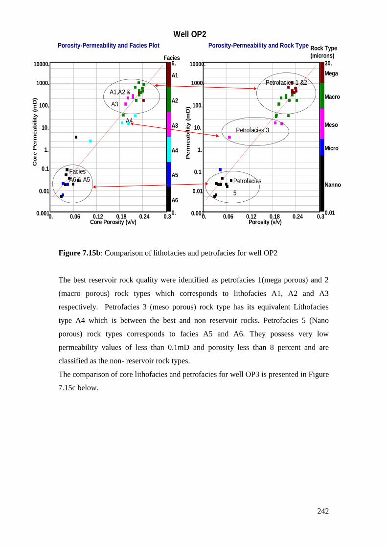
242

Figure 7.15b: Comparison of lithofacies and petrofacies for well OP2

The best reservoir rock quality were identified as petrofacies 1(mega porous) and 2

(macro porous) rock types which corresponds to lithofacies A1, A2 and A3

respectively. Petrofacies 3 (meso porous) rock type has its equivalent Lithofacies

type A4 which is between the best and non reservoir rocks. Petrofacies 5 (Nano

porous) rock types corresponds to facies A5 and A6. They possess very low

permeability values of less than 0.1mD and porosity less than 8 percent and are

classified as the non- reservoir rock types.

The comparison of core lithofacies and petrofacies for well OP3 is presented in Figure

7.15c below.


0. 0.06 0.12 0.18 0.24 0.3Core Porosity (v/v)

0.001

0.01

0.1

1.

10.

100.

1000.

10000.

Co

re P

erm

eab

ilit

y (

mD

)

A6

A5

A4

A3

A2

A1

0.

6.Facies

Facies

A6 & A5

A1,A2 &

A3

A4

Well OP2

Porosity-Permeability and Rock Type

0. 0.06 0.12 0.18 0.24 0.3Porosity (v/v)

0.001

0.01

0.1

1.

10.

100.

1000.

10000.

Perm

eab

ilit

y (

mD

)Nanno

Micro

Meso

Macro

Mega

0.01

30.

Rock Type

(microns)

Petrofacies 1 &2

Petrofacies 3

Petrofacies

5

243

Figure 7.15c: Comparison of lithofacies and petrofacies for well OP3

In well OP3, four petrofacies (macro, meso, micro, and Nanno porous) rock types and

four Lithofacies (A3, A4, A5 and A6) were identified as shown above. The best

reservoir quality rock in terms of petrofacies is petrofacies 2 (macro porous) rock

types which has an equivalent lithofacies as facies A3. This rock type is closely

followed by petrofacies 3(meso porous) that corresponds to facies A4. The non

reservoir rock (facies A6) has petrofacies 4 and 5 (micro and Nano porous) rock types

as its equivalent rock.

Generally, lithofacies with the best characteristics (A1 and A2) correspond to the best

quality rock (Petrofacies 1), and non reservoir rock (Petrofacies 5) corresponds to

facies A6. It is important to note that lithofacies were classified based on grain size

and texture of the cores, Petrofacies were determined based upon the analysis of the

pore system of the rock.

The comparison between lithofacies and petrofacies indicates that within a given

lithofacies, there may exist different Petrofacies which are indicative of rock quality.

Figure 7.15 below presents the comparison of core lithofacies and petrofacies for all

wells.


0. 0.06 0.12 0.18 0.24 0.3Core Porosity (v/v)

0.001

0.01

0.1

1.

10.

100.

1000.

Co

re P

erm

eab

ilit

y (

mD

)

A6

A5

A4

A3

A2

A1

0.

6.Facies

Facies

A6

Facies

A3 & A4

Well OP3

Porosity-Permeability and Rock Type Plot

0. 0.06 0.12 0.18 0.24 0.3Porosity (v/v)

0.001

0.01

0.1

1.

10.

100.

1000.

Perm

eab

ilit

y (

mD

)

Nanno

Micro

Meso

Macro

Mega

0.01

30.

Rock Type

Petrofacies 2

&3

Petrofacies

3,4 &5

244

Figure 7.15d: Comparison of lithofacies and petrofacies for all the wells

7.7 K/PHI RELATION

The ratio of the permeability to porosity plot is a useful indicator of flow quality and

storage capacity of rocks. It reflects quality of rock expressed in terms of flow

efficiency.

When pore systems are dependent on grain size, the plot of porosity versus

permeability provides a direct relationship. The plot of porosity versus permeability

ratio helps to know the differences in rock types in relation to diagenesis and flow

capacity of the rock. The porosity permeability ratios used in this study are as follows

K/PHI=0.01

K/PHI=0.05

K/PHI=0.5

K/PHI =5

K/PHI=50

The graphics below (Figure 7.15e) is the result of the application of the above

porosity and permeability ratio and Winland pore throat radius for all the wells.


0. 0.06 0.12 0.18 0.24 0.3

Core Porosity (v/v)

0.001

0.01

0.1

1.

10.

100.

1000.

10000.

Co

re P

erm

eab

ilit

y (

mD

)

A6

A5

A4

A3

A2

A1

0.

6.Facies

Well

OP1

OP2

OP3

A5 & A6

A1 &A2

A3 & A4

All WellPorosity-Permeability and Rock Type Plot

0. 0.06 0.12 0.18 0.24 0.3

Porosity (v/v)

0.001

0.01

0.1

1.

10.

100.

1000.

10000.

Perm

eab

ilit

y (

mD

)

Nanno

Micro

Meso

Macro

Mega

0.01

30.

Rock Type

Petrofacies

1

Petrofacies 2

&3

Petrofacies

4 & 5

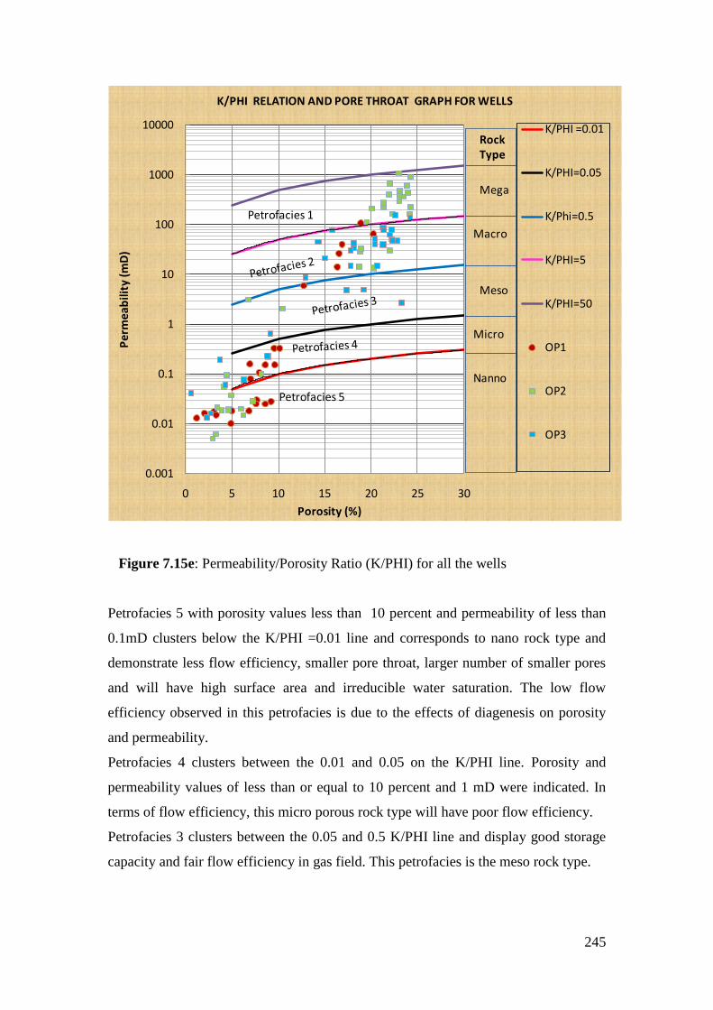
245

0.001

0.01

0.1

1

10

100

1000

10000

0 5 10 15 20 25 30

Pe

rme

abil

ity

(mD

)

Porosity (%)

K/PHI RELATION AND PORE THROAT GRAPH FOR WELLS

K/PHI =0.01

K/PHI=0.05

K/Phi=0.5

K/PHI=5

K/PHI=50

OP1

OP2

OP3

Petrofacies 1

Petrofacies 5

RockType

Mega

Macro

Meso

Micro

Nanno

Figure 7.15e: Permeability/Porosity Ratio (K/PHI) for all the wells

Petrofacies 5 with porosity values less than 10 percent and permeability of less than

0.1mD clusters below the K/PHI =0.01 line and corresponds to nano rock type and

demonstrate less flow efficiency, smaller pore throat, larger number of smaller pores

and will have high surface area and irreducible water saturation. The low flow

efficiency observed in this petrofacies is due to the effects of diagenesis on porosity

and permeability.

Petrofacies 4 clusters between the 0.01 and 0.05 on the K/PHI line. Porosity and

permeability values of less than or equal to 10 percent and 1 mD were indicated. In

terms of flow efficiency, this micro porous rock type will have poor flow efficiency.

Petrofacies 3 clusters between the 0.05 and 0.5 K/PHI line and display good storage

capacity and fair flow efficiency in gas field. This petrofacies is the meso rock type.

246

Petrofacies 2 indicates good flow efficiency and larger pore throats and smaller

number of larger pores. These facies have lower irreducible water saturations and

smaller surface areas. They cluster between the 0.5 and 5 on the K/PHI line.

Petrofacies 1 indicate high flow efficiency and cluster between 5 and 50 on the K/PHI

line. The porosity of this facies is between 15 and 25 % which represents a high

storage capacity. Flow depends more on permeability than porosity and petrofacies 1

showed permeability values in the range of 85 to 1000 mD. Larger pore throat and

low irreducible water saturation play a dominant role in this petrofacies.

7.8 HYDRAULIC FLOW ZONE INDICATOR (FZI)

A Petrophysical flow unit is defined as an interval of sediment with similar

petrophysical properties such as porosity, permeability, water saturation, pore throat

radius, storage and flow capacity, that are different from the intervals immediately

above and below the reservoir intervals (Porras and Campos, 2001). Petrophysical

flow units are usually grouped and used in determination of reservoir flow units.

Bear (1972) defined Hydraulic flow units as the representative of elementary volume

of the total reservoir rock within which geological and petrophysical properties that

affect fluid flow are internally consistent and predictably different from properties of

other rock volumes.

Amaefule et al. (1993) showed that it is not possible to get good reservoir description

without introducing pore throat parameters and bridging the gap between microscopic

attributes from routine core plugs and macroscopic log derived characterization and

they introduced the concept of reservoir quality index (RQI) to define the pattern of

flow units. The hydraulic flow unit concept (Amaefule et al., 1993) is adopted in this

work to identify reservoir rock quality and heterogeneity. The method can be applied

to carbonate reservoirs as well as to clastic rocks by subdividing the reservoir into

distinct petrophysical types. Each distinct reservoir unit has a unique flow zone

indicator (FZI), Reservoir quality index (RQI), and Normalized Porosity Index (NPI)

values (Al-Dhafeeri &Nasr-El-Din, 2006).

The combination of porosity and permeability data in terms of flow zone indicator,

reservoir quality index, and normalized porosity index is convenient to use with

routine core analysis data. The concept of Amaefule et al. (2003) is based on the

calculation of two terms, RQI and NPI as defined below:

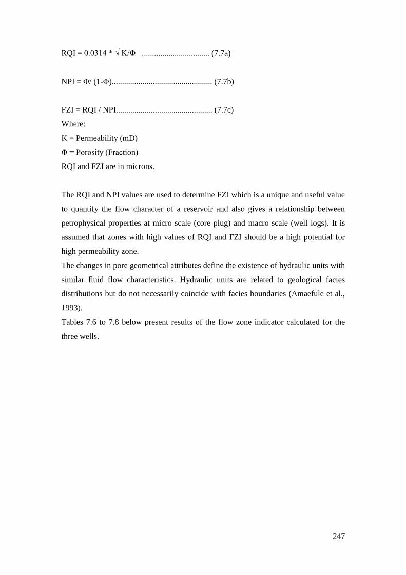
247

RQI = 0.0314 * √ K/Φ ................................. (7.7a)

NPI = Φ/ (1-Φ)................................................. (7.7b)

FZI = RQI / NPI............................................... (7.7c)

Where:


Φ = Porosity (Fraction)

RQI and FZI are in microns.

The RQI and NPI values are used to determine FZI which is a unique and useful value

to quantify the flow character of a reservoir and also gives a relationship between

petrophysical properties at micro scale (core plug) and macro scale (well logs). It is

assumed that zones with high values of RQI and FZI should be a high potential for

high permeability zone.

The changes in pore geometrical attributes define the existence of hydraulic units with

similar fluid flow characteristics. Hydraulic units are related to geological facies

distributions but do not necessarily coincide with facies boundaries (Amaefule et al.,

1993).

Tables 7.6 to 7.8 below present results of the flow zone indicator calculated for the

three wells.

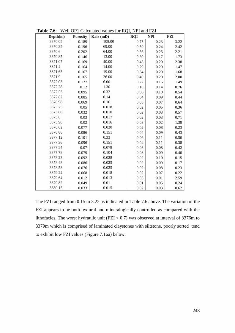
248

Table 7.6: Well OP1 Calculated values for RQI, NPI and FZI

Depth(m) Porosity Kair (mD) RQI NPI FZI

3370.05 0.189 108.00 0.75 0.23 3.22

3370.35 0.196 69.00 0.59 0.24 2.42

3370.6 0.202 64.00 0.56 0.25 2.21

3370.85 0.146 13.00 0.30 0.17 1.73

3371.07 0.169 40.00 0.48 0.20 2.38

3371.4 0.164 14.00 0.29 0.20 1.47

3371.65 0.167 19.00 0.34 0.20 1.68

3371.9 0.165 26.00 0.40 0.20 2.00

3372.03 0.127 6.00 0.22 0.15 1.49

3372.28 0.12 1.30 0.10 0.14 0.76

3372.53 0.095 0.32 0.06 0.10 0.54

3372.82 0.085 0.14 0.04 0.09 0.44

3378.98 0.069 0.16 0.05 0.07 0.64

3373.75 0.05 0.018 0.02 0.05 0.36

3373.88 0.032 0.010 0.02 0.03 0.57

3375.6 0.03 0.017 0.02 0.03 0.71

3375.98 0.02 0.016 0.03 0.02 1.38

3376.62 0.077 0.030 0.02 0.08 0.23

3376.86 0.086 0.151 0.04 0.09 0.43

3377.12 0.101 0.33 0.06 0.11 0.50

3377.36 0.096 0.151 0.04 0.11 0.38

3377.54 0.07 0.079 0.03 0.08 0.42

3377.78 0.079 0.104 0.03 0.09 0.40

3378.23 0.092 0.028 0.02 0.10 0.15

3378.48 0.086 0.025 0.02 0.09 0.17

3378.58 0.076 0.025 0.02 0.08 0.23

3379.24 0.068 0.018 0.02 0.07 0.22

3379.64 0.012 0.013 0.03 0.01 2.59

3379.82 0.049 0.01 0.01 0.05 0.24

3380.15 0.033 0.015 0.02 0.03 0.62

The FZI ranged from 0.15 to 3.22 as indicated in Table 7.6 above. The variation of the

FZI appears to be both textural and mineralogically controlled as compared with the

lithofacies. The worst hydraulic unit (FZI < 0.7) was observed at interval of 3376m to

3379m which is comprised of laminated claystones with siltstone, poorly sorted tend

to exhibit low FZI values (Figure 7.16a) below.

249

Well OP1

Flow zone Indicator Vs Depth and Rock Type

0.01 1.008 2.006 3.004 4.002 5.

Flow Zone Indicator (FZI)

3382.

3378.8

3375.6

3372.4

3369.2

3366.

Dep

th (m

)

Nanno

Micro

Meso

Macro

Mega

0.01

30.

Rock Type

FZI< 0.7 = Claystones

FZI

>1.5=Sandstones

OP1Scale : 1 : 200


DEPTH

(M)







3375

Facies A3

Facies A4

Facies A5

Facies A4

Facies A6

3380

3380

Sandstones

Shale

Figure 7.16a: Well OP1 flow zone indicator, rock types and facies plot

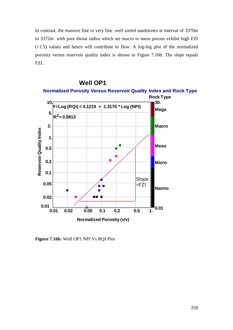
250

In contrast, the massive fine to very fine ,well sorted sandstones at interval of 3370m

to 3372m with pore throat radius which are macro to meso porous exhibit high FZI

(>1.5) values and hence will contribute to flow. A log-log plot of the normalized

porosity versus reservoir quality index is shown in Figure 7.16b. The slope equals

FZI.

Well OP1

Normalized Porosity Versus Reservoir Quality Index and Rock Type

0.01 0.02 0.05 0.1 0.2 0.5 1.

Normalized Porosity (v/v)

0.01

0.02

0.05

0.1

0.2

0.5

1.

2.

5.

10.

Reserv

oir

Qu

ality

Ind

ex

Nanno

Micro

Meso

Macro

Mega

0.01

30.

Rock Type

Y=Log (RQI) = 0.1219 + 1.3170 * Log (NPI)

R2= 0.5813

Slope

=FZI

Figure 7.16b: Well OP1 NPI Vs RQI Plot

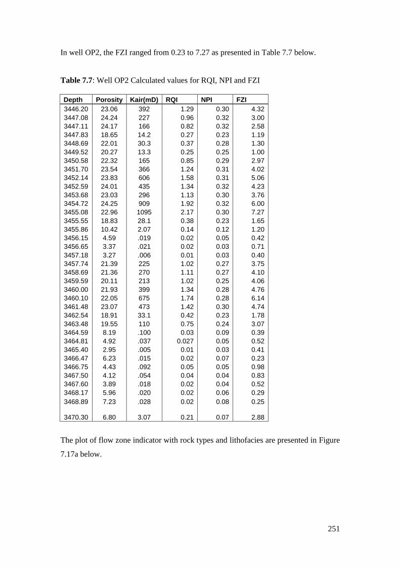
251

In well OP2, the FZI ranged from 0.23 to 7.27 as presented in Table 7.7 below.


Depth Porosity Kair(mD) RQI NPI FZI

3446.20 23.06 392 1.29 0.30 4.32

3447.08 24.24 227 0.96 0.32 3.00

3447.11 24.17 166 0.82 0.32 2.58

3447.83 18.65 14.2 0.27 0.23 1.19

3448.69 22.01 30.3 0.37 0.28 1.30

3449.52 20.27 13.3 0.25 0.25 1.00

3450.58 22.32 165 0.85 0.29 2.97

3451.70 23.54 366 1.24 0.31 4.02

3452.14 23.83 606 1.58 0.31 5.06

3452.59 24.01 435 1.34 0.32 4.23

3453.68 23.03 296 1.13 0.30 3.76

3454.72 24.25 909 1.92 0.32 6.00

3455.08 22.96 1095 2.17 0.30 7.27

3455.55 18.83 28.1 0.38 0.23 1.65

3455.86 10.42 2.07 0.14 0.12 1.20

3456.15 4.59 .019 0.02 0.05 0.42

3456.65 3.37 .021 0.02 0.03 0.71

3457.18 3.27 .006 0.01 0.03 0.40

3457.74 21.39 225 1.02 0.27 3.75

3458.69 21.36 270 1.11 0.27 4.10

3459.59 20.11 213 1.02 0.25 4.06

3460.00 21.93 399 1.34 0.28 4.76

3460.10 22.05 675 1.74 0.28 6.14

3461.48 23.07 473 1.42 0.30 4.74

3462.54 18.91 33.1 0.42 0.23 1.78

3463.48 19.55 110 0.75 0.24 3.07

3464.59 8.19 .100 0.03 0.09 0.39

3464.81 4.92 .037 0.027 0.05 0.52

3465.40 2.95 .005 0.01 0.03 0.41

3466.47 6.23 .015 0.02 0.07 0.23

3466.75 4.43 .092 0.05 0.05 0.98

3467.50 4.12 .054 0.04 0.04 0.83

3467.60 3.89 .018 0.02 0.04 0.52

3468.17 5.96 .020 0.02 0.06 0.29

3468.89 7.23 .028 0.02 0.08 0.25

3470.30 6.80 3.07 0.21 0.07 2.88

The plot of flow zone indicator with rock types and lithofacies are presented in Figure

7.17a below.

252

OP2Scale : 1 : 200


2

DEPTH

(M)

5

GR (GAPI)0. 150.

7



11



12

Cor Kair (mD)0.001 10000.

3450

3475

Facies A1

Facies A2

Facies A3

Facies A4

Facies A3

Facies A5

Facies A4

Facies A2

Facies A6

Well OP2

Flow Zone Indicator Vs Depth and

Rock Type Plot

0.01 2.008 4.006 6.004 8.002 10.


3472.

3466.4

3460.8

3455.2

3449.6

3444.

Dep

th (m

)

Nanno

Micro

Meso

Macro

Mega

0.01

30.

Rock Type

3460

Massive

Sands

Massive

Sands

Shale


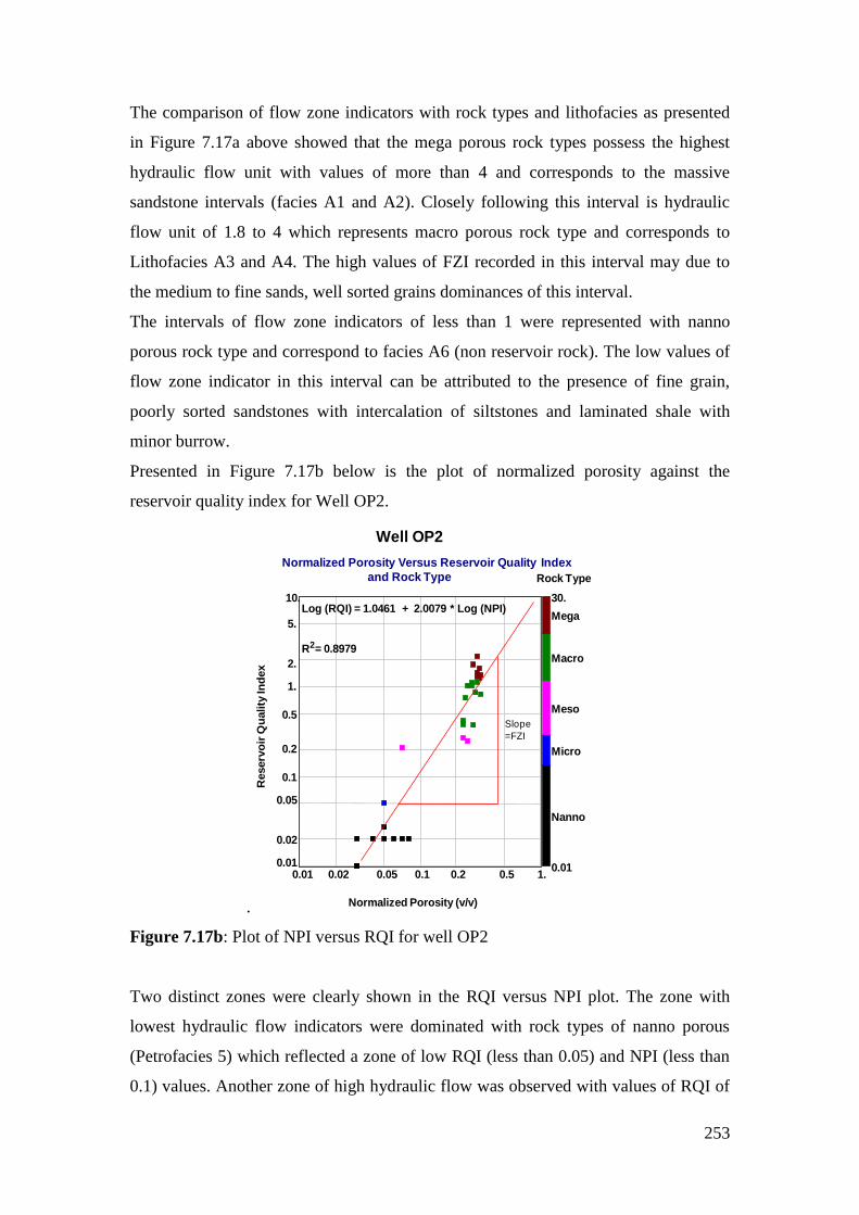
253

The comparison of flow zone indicators with rock types and lithofacies as presented

in Figure 7.17a above showed that the mega porous rock types possess the highest

hydraulic flow unit with values of more than 4 and corresponds to the massive

sandstone intervals (facies A1 and A2). Closely following this interval is hydraulic

flow unit of 1.8 to 4 which represents macro porous rock type and corresponds to

Lithofacies A3 and A4. The high values of FZI recorded in this interval may due to

the medium to fine sands, well sorted grains dominances of this interval.

The intervals of flow zone indicators of less than 1 were represented with nanno

porous rock type and correspond to facies A6 (non reservoir rock). The low values of

flow zone indicator in this interval can be attributed to the presence of fine grain,

poorly sorted sandstones with intercalation of siltstones and laminated shale with

minor burrow.

Presented in Figure 7.17b below is the plot of normalized porosity against the

reservoir quality index for Well OP2.

.

Well OP2

Normalized Porosity Versus Reservoir Quality Index

and Rock Type

0.01 0.02 0.05 0.1 0.2 0.5 1.


0.01

0.02

0.05

0.1

0.2

0.5

1.

2.

5.

10.

Reserv

oir

Qu

ality

In

dex

Nanno

Micro

Meso

Macro

Mega

0.01

30.

Rock Type

Log (RQI) = 1.0461 + 2.0079 * Log (NPI)

R2= 0.8979

Slope

=FZI

Figure 7.17b: Plot of NPI versus RQI for well OP2

Two distinct zones were clearly shown in the RQI versus NPI plot. The zone with

lowest hydraulic flow indicators were dominated with rock types of nanno porous

(Petrofacies 5) which reflected a zone of low RQI (less than 0.05) and NPI (less than

0.1) values. Another zone of high hydraulic flow was observed with values of RQI of

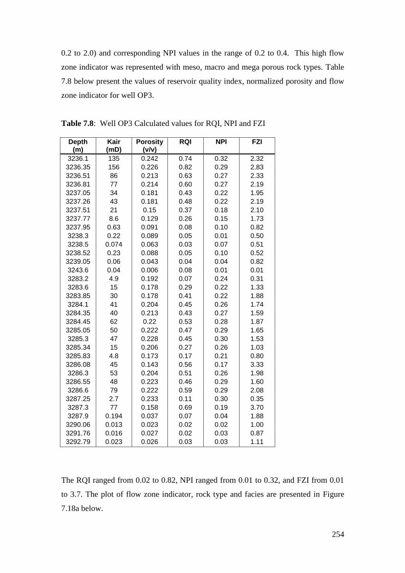
254

0.2 to 2.0) and corresponding NPI values in the range of 0.2 to 0.4. This high flow

zone indicator was represented with meso, macro and mega porous rock types. Table

7.8 below present the values of reservoir quality index, normalized porosity and flow

zone indicator for well OP3.


Depth

(m) Kair (mD)

Porosity (v/v)

RQI NPI FZI

3236.1 135 0.242 0.74 0.32 2.32

3236.35 156 0.226 0.82 0.29 2.83

3236.51 86 0.213 0.63 0.27 2.33

3236.81 77 0.214 0.60 0.27 2.19

3237.05 34 0.181 0.43 0.22 1.95

3237.26 43 0.181 0.48 0.22 2.19

3237.51 21 0.15 0.37 0.18 2.10

3237.77 8.6 0.129 0.26 0.15 1.73

3237.95 0.63 0.091 0.08 0.10 0.82

3238.3 0.22 0.089 0.05 0.01 0.50

3238.5 0.074 0.063 0.03 0.07 0.51

3238.52 0.23 0.088 0.05 0.10 0.52

3239.05 0.06 0.043 0.04 0.04 0.82

3243.6 0.04 0.006 0.08 0.01 0.01

3283.2 4.9 0.192 0.07 0.24 0.31

3283.6 15 0.178 0.29 0.22 1.33

3283.85 30 0.178 0.41 0.22 1.88

3284.1 41 0.204 0.45 0.26 1.74

3284.35 40 0.213 0.43 0.27 1.59

3284.45 62 0.22 0.53 0.28 1.87

3285.05 50 0.222 0.47 0.29 1.65

3285.3 47 0.228 0.45 0.30 1.53

3285.34 15 0.206 0.27 0.26 1.03

3285.83 4.8 0.173 0.17 0.21 0.80

3286.08 45 0.143 0.56 0.17 3.33

3286.3 53 0.204 0.51 0.26 1.98

3286.55 48 0.223 0.46 0.29 1.60

3286.6 79 0.222 0.59 0.29 2.08

3287.25 2.7 0.233 0.11 0.30 0.35

3287.3 77 0.158 0.69 0.19 3.70

3287.9 0.194 0.037 0.07 0.04 1.88

3290.06 0.013 0.023 0.02 0.02 1.00

3291.76 0.016 0.027 0.02 0.03 0.87

3292.79 0.023 0.026 0.03 0.03 1.11

The RQI ranged from 0.02 to 0.82, NPI ranged from 0.01 to 0.32, and FZI from 0.01

to 3.7. The plot of flow zone indicator, rock type and facies are presented in Figure

7.18a below.

255

OP3Scale : 1 : 200


2

DEPTH

(M)

3

GRn (GAPI)0. 150.

4


6


Cor Poro ()0.5 0.

7

Cor Klin ()0.001 1000.

8

CoreSw w ()0. 100.

3230

3240

Facies A3

Facies A4

Facies A5

Facies A6

OP3Scale : 1 : 200


3270

3280

3290

Facies A3

Facies A4

Facies A5

Facies A6

Facies A4

Facies A3

Facies A6

Massive

Sand

Shaly/

Silt

Sand

Shaly

Well OP3

Flow Zone Indicator Vs Dept

and Rock Type

0.001 1.0008 2.0006 3.0004 4.0002 5.


3294.

3281.2

3268.4

3255.6

3242.8

3230.

Dep

th (m

)

Nanno

Micro

Meso

Macro

Mega

0.01

30.

Rock Type


256

The FZI values in the range of 1.6 to 3.7 represent the massive sandstone intervals

and correspond to rock types of predominantly macro porous and facies A3 and A4

respectively and have potential for productivity. Intervals of with FZI values of less

than 1 represent the shaly/silt and shale intervals and correspond to meso, micro and

nano porous rock types. The equivalent facies is facies A5 and A6. This interval of

low flow zone indicators were regarded as the un-productive intervals based on flow

zone indicators. The low values of FZI recorded may be attributed to the pore lining,

pore filling and pore bridging clays as well as fine grained that are poorly sorted as

confirmed in the petrography study results.

The log-log cross plot of normalized porosity versus the reservoir quality index is

presented in Figure 7.18b below.

Well OP3


and Rock type

0.01 0.02 0.05 0.1 0.2 0.5 1.


0.01

0.1

1.

10.

100.

Reserv

oir

Qu

ality

Ind

ex

Nanno

Micro

Meso

Macro

Mega

0.01

30.

Rock Type

Log(RQI) = 0.1117 + 0.9459 * Log(NPI)

R2= 0.6455

Figure 7.18b: Plot of NPI Versus RQI for well OP3

A regression analysis correlation coefficient of 0.6 was obtained from the cross plot

which portray a good agreement between the plotted data. The slope of the plot gives

the flow zone indicator.

The plot of normalized porosity and reservoir quality index for all the well is

presented in the Figure below.

257

All Well


and Rock Type

0.01 0.02 0.05 0.1 0.2 0.5 1.


0.01

0.02

0.05

0.1

0.2

0.5

1.

2.

5.

10.

Reserv

oir

Qu

ality

In

dex

Nanno

Micro

Meso

Macro

Mega

0.01

30.

Rock Type

Log(RQI) = 0.5992 + 1.5614 * Log(NPI)

R2= 0.7355

Figure 7.18c: Plot of NPI Versus RQI for Well OP3

The mega porous rocks showed high values of RQI (1 to 2) and NPI (25 % to 32 %)

which represent the best reservoir rock quality of the wells studied. The poor reservoir

rock quality was observed in the nanno and micro porous rock types which showed

values of RQI and NPI of less than 0.1 respectively. A good regression analysis

coefficient of correlation of 73 % was realized from the cross plot.

258

CHAPTER EIGHT

DETERMINATION OF FLUID CONTACT

8.1 INTRODUCTION

The identification of fluid in rocks and possible contacts provides useful information

on the petrophysical interpretation. Oil and gas are both fluid and pressure is one of

the important elements in characterising the physical behaviours of fluids in the

subsurface. The water contact is used to describe the elevation above which fluids

(oil/gas) can be found in the pores of the rock. The fluid contacts can be determined

by petrophysical interpretation of wire logs and production test results. Oil finger

printing of residual hydrocarbons from sidewall core extracts can also provide an

independent means of identification of reservoir fluid types.

As hydrocarbon and water accumulates in a reservoir, separation occurs as a result of

the difference in the specific gravity of various fluids. The less dense fluid like gas

rise to the top of the reservoir, and below the gas is a gas to oil transition zone. Below

the transition zone in most reservoirs is an oil-water transition zone of varying

thickness which is partly filled with oil and water. Beneath the oil-water transition

zone is the part of the formation that is completely saturated with water (Link, 1982).

An assessment of the pore fluid types and contacts has been undertaken based on

wireline pressure data, log data and saturation estimates from logs as presented in the

subsections below.

8.2 WIRELINE PRESSURE DATA ANALYSIS AND INTERPRETATION

Pressure is defined as the measure of force per unit area. Pressure in the subsurface is

a function of the densities of the rock and fluids. The normal hydrostatic pressure

increases with depth and the rate of pressure change depends only on water density.

The pressure-depth relationship is independent of the shape of the fluid container

(Dahlberg, 1994). Fluid density is the controlling factor in the normal hydrostatic

pressure gradient.

The Table 8.1 below shows typical density ranges and gradients for gas, oil and water

that vary with pressure, temperature and composition.

259

Table 8.1: Ranges of density and pressure gradients for hydrocarbon.

Fluid Normal density

range (g/cm3)

Gradient range

(psi/ft)

Gas (gaseous) 0.007-0.30 0.003-1.130

Gas (liquid) 0.200-0.40 0.090-0.174

Oil 0.400-1.12 0.174-0.486

Water 1.000-1.15 0.433-0.500

(Modified after, Gearhart-Owens Industry, 1972)

The wireline pressure data were acquired in some of the wells in the study area in

order to establish fluid pressure gradients in several reservoir sands in the study area.

The results of the repeat formation tests for wells are given in appendix K. the

pressure test may be unsuccessful due to packer seal failure, flow line or probe

blockages, poor isolation of the mud column or tight formation. In very low

permeability environments, formation layers may become “supercharges” by mud

filtrate invasion and pressure points will plot on the high side of the normal pressure

gradient line. The supercharged points are neglected in the pressure depth plot

because they are not reliable.

The interpretation is performed by constructing pressure versus depth plot to

establish pressure distribution and fluid gradients. The intersection of hydrocarbon

and water gradients is used to identify the free water level and also define the contact.

The fluid densities were deduced from the pressure gradient using the following

relationship (Bateman, 1985):

Fluid density (g/cc) = Pressure gradient (psi/ft) * 2.3072..................... (8.1)

However, equation 8.1 above was modified to express the pore pressure gradients in

psi/m using the following equivalent relationship:

1 psi/m = 0.7034 g/cc

The RFT was run in eight wells by Schlumberger Company. Gas and water gradients

were identified in many of the wells with some variations.

260

8.2.1 Well OP1

The RFT tool was run in well OP1 to establish formation pressures and fluid gradients

in reservoir sands and to obtain a qualitative indication of permeability. However,

within the Albian age of the formation, a total of twelve RFT formation pressure tests

were measured on well OP1 as presented in appendix K. An interpretation of the

result is presented in Figure 8.1 below.

Figure 8.1: Well OP1 pressure versus depth plot for identification of Gas/Water

contact (GWC) and fluid densities.

The Figure above present two separate reservoirs of well OP1 using the pressure-

depth plot from the repeat formation test measurements (RFT). A communication in

aquifer between the two reservoir intervals is represented in the water gradient line

(blue) with water density of 1.02 g/cc.

Two gas gradients of 0.16g/cc and 0.17g/cc were calculated from the slope of the plot

in the two sandstone intervals. Two Possible gas water contacts (GWC) were

Well OP1

Pressure Versus Depth Plot (RFT)

4800. 4860. 4920. 4980. 5040. 5100.

Pressure (psig)

3450.

3420.

3390.

3360.

3330.

3300.

De

pth

(m

)

Water gradient = 1.45 psi/m= 1.02 g/cc

Gas gradient

= 0.23 psi/m =0.16 g/cc

Gas gradient

= 0.24 psi/m

=0.17 g/cc

GWC =3376m

GWC =3407.4m

Well OP1

Pressure Versus Depth Plot (RFT)

4800. 4860. 4920. 4980. 5040. 5100.

Pressure (psig)

3450.

3420.

3390.

3360.

3330.

3300.

De

pth

(m

)

Water gradient = 1.45 psi/m= 1.02 g/cc

Gas gradient

= 0.23 psi/m =0.16 g/cc

Gas gradient

= 0.24 psi/m

=0.17 g/cc

GWC =3376m

GWC =3407.4m

261

identified at measured depth of 3376m and 3407.4m respectively. This result will be

confirmed with the log data.

8.2.2 Well OP2

A total of seventeen RFT pressure test measurements were performed within the

measured depth interval of 3300m to 3460m as presented in appendix K. The

interpretation is presented in Figure 8.2 below.

1.65 psi/m

=1.16g/cc

Well OP2

Formation Pressure Vs Depth

Interval : 3300- 3460m.

4850. 4920. 4990. 5060. 5130. 5200.

Formation Pressure (psi)

3460.

3428.

3396.

3364.

3332.

3300.

Dep

th (m

)

Water gradient

=1.46 psi /m = 1.02 g/cc

Figure 8.2: Well OP2 pressure versus depth plot

The pressure point that fall on the left of the water gradient line between the interval

of 3300m to 3332m may be due to slow pressure build up or to the RFT temperature

stabilization. A water gradient of 1.46 psi/m which is equal to water density of 1.02

g/cc represents a water productive reservoir interval. No gas/water contact was

identified in this well.

262

8.2.3 Well OP3

In well OP3, a total of twenty three (23) RFT pressure test measurements were

performed. The mud pressure data was corrected to the formation pressure, and a mud

weight of approximately 2lb/gal was recorded. The interpreted result is presented in

Figure 8.3 below.

1.41 psi/m

=0.99 g/cc

0.492 psi/m

=0.34g/cc

1.41 psi/m

=0.99 g/cc

Well OP3 Sand 3

(3353 -3373 m)


4700. 4770. 4840. 4910. 4980. 5050.

Formation Pressure(psi)

3380.

3373

3366

3359

3352

3346.

De

pth

(m

)

Well OP3


4700. 4770. 4840. 4910. 4980. 5050.

Formation Pressure(psi)

3380.

3346.

3312.

3278.

3244.

3210.

Dep

th (m

)

Gas

gradient=0.

22 psi/m

=0.15 g/cc Water

gradient=1.39

psi/m =0.98 g/cc

0.98 g/cc

0.15

g/cc

GWC=3361.3m

Figure 8.3: Well OP3 pressure versus depth plot showing possible gwc at measured

depth 3361.3m

Two separate gas columns at measured between the interval of 3210 -3244m and 3278

-3312m were observed as shown in the Figure above. A possible gas-water contact at

measured depth of 3361.3m was observed. A calculated water density of 0.98 g/cc

and gas density of 0.15 g/cc were obtained from the slope of the plot.

8.2.4 Well OP4

A total of nineteen RFT pressure test measurements were performed between the inter

val of 3200m to 3350m as shown in appendix K. A supercharged pressure was also

observed. The interpretation of the result is as shown in Figure 8.4 below.

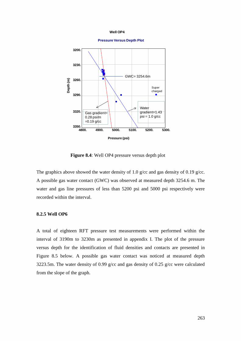
263

Well OP4

Pressure Versus Depth Plot

4800. 4900. 5000. 5100. 5200. 5300.

Pressure (psi)

3350.

3320.

3290.

3260.

3230.

3200.

Dep

th (m

)

Super

charged

Water

gradient=1.43

psi = 1.0 g/ccGas gradient=

0.28 psi/m

=0.19 g/cc

GWC= 3254.6m


The graphics above showed the water density of 1.0 g/cc and gas density of 0.19 g/cc.

A possible gas water contact (GWC) was observed at measured depth 3254.6 m. The

water and gas line pressures of less than 5200 psi and 5000 psi respectively were

recorded within the interval.

8.2.5 Well OP6

A total of eighteen RFT pressure test measurements were performed within the

interval of 3190m to 3230m as presented in appendix I. The plot of the pressure

versus depth for the identification of fluid densities and contacts are presented in

Figure 8.5 below. A possible gas water contact was noticed at measured depth

3223.5m. The water density of 0.99 g/cc and gas density of 0.25 g/cc were calculated

from the slope of the graph.

264

Well OP 6


4600. 4620. 4640. 4660. 4680. 4700.

Pressure (psi)

3230.

3222.

3214.

3206.

3198.

3190.

DE

PT

H

Water gradient =1.42 psi/m

= 0.99 g/cc

Gas

gradient =

0.36 psi/m

=0.25 g/cc

GWC = 3223m


8.2.6 Well MA1

A total of eleven RFT formation pressure test measurements were obtained within the

Albian age sandstone reservoir interval of well MA1. The results are presented in

appendix K. Shown in Figure 8.6 below is the pressure versus depth plot. The

pressure versus depth interval investigated in well MA1 indicated wet sandstone

reservoir interval with a gradient of 1.02 g/cc. No gas was intersected in this analysis.

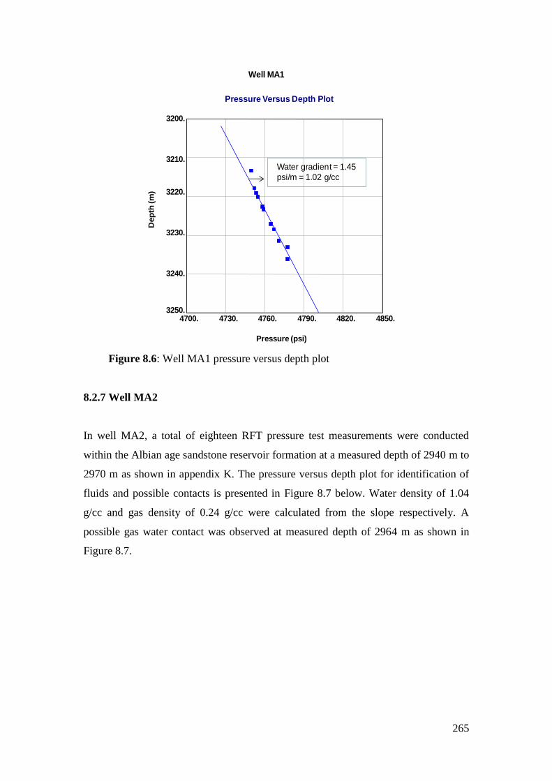
265

Well MA1


4700. 4730. 4760. 4790. 4820. 4850.

Pressure (psi)

3250.

3240.

3230.

3220.

3210.

3200.

Dep

th (m

)

Water gradient = 1.45

psi/m = 1.02 g/cc

Figure 8.6: Well MA1 pressure versus depth plot

8.2.7 Well MA2

In well MA2, a total of eighteen RFT pressure test measurements were conducted

within the Albian age sandstone reservoir formation at a measured depth of 2940 m to

2970 m as shown in appendix K. The pressure versus depth plot for identification of

fluids and possible contacts is presented in Figure 8.7 below. Water density of 1.04

g/cc and gas density of 0.24 g/cc were calculated from the slope respectively. A

possible gas water contact was observed at measured depth of 2964 m as shown in

Figure 8.7.

266


8.2.8 Well MA3

A total of nine successful RFT pressure test measurements were performed within the

depth range of 2936m to 3080m of well MA3 as shown in appendix K. The

interpretation of the result is presented in Figure 8.8 below.

0.638

psi/m=0.45

g/cc

Well MA2


4350. 4364. 4378. 4392. 4406. 4420.


2970.

2964.

2958.

2952.

2946.

2940.

Depth (m)

Water gradient =1.48

psi/m = 1.04 g/cc

Gas gradient

=0.35 psi/m

=0.24 g/cc

GWC = 2964m

267


The aquifer density obtained from the calculation was 1.17 g/cc and gas density of 0.3

g/cc respectively. A possible gas water contact was also observed at measured depth

of 3069m. The Table 8.2 below summaries the interpreted water and gas gradients

interpreted in each well from the pressure data.

Table 8.2: Summary of pressure gradients and densities for Wells

Well Water

Gradient

(psi/m)

Water

Gradient

(psi/ft)

Density

(g/cc)

Gas

Gradient

(psi/m)

Gas

Gradient

(psi/ft)

Density

(g/cc)

OP1 1.45 0.44 1.02 0.23 0.07 0.16

OP2 1.46 0.44 1.02 - - -

OP3 1.39 0.42 0.98 0.22 0.07 0.15

OP4 1.43 0.44 1.00 0.28 0.09 0.19

OP6 1.42 0.43 0.99 0.36 0.11 0.25

MA1 1.45 0.44 1.02 - - -

MA2 1.48 0.45 1.04 0.35 0.11 0.24

MA3 1.67 0.51 1.20 0.44 0.13 0.3

Average 1.44 0.44 1.02 0.29 0.09 0.20

1.7 psi/m = 1.2 g/cc

Well MA3


4350. 4410. 4470. 4530. 4590. 4650.


3080.

3044.

3008.

2972.

2936.

2900.

De

pth

(m

)

Water gradient = 1.67 psi/m

= 1.2 g/cc

Gas gradient

=0.44 psi /m

=0.3 g/cc

GWC =3069.m

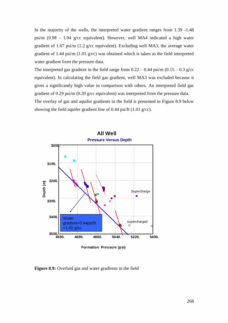
268

In the majority of the wells, the interpreted water gradient ranges from 1.39 -1.48

psi/m (0.98 – 1.04 g/cc equivalent). However, well MA4 indicated a high water

gradient of 1.67 psi/m (1.2 g/cc equivalent). Excluding well MA3, the average water

gradient of 1.44 psi/m (1.01 g/cc) was obtained which is taken as the field interpreted

water gradient from the pressure data.

The interpreted gas gradient in the field range from 0.22 – 0.44 psi/m (0.15 – 0.3 g/cc

equivalent). In calculating the field gas gradient, well MA3 was excluded because it

gives a significantly high value in comparison with others. An interpreted field gas

gradient of 0.29 psi/m (0.20 g/cc equivalent) was interpreted from the pressure data.

The overlay of gas and aquifer gradients in the field is presented in Figure 8.9 below

showing the field aquifer gradient line of 0.44 psi/ft (1.01 g/cc).

Figure 8.9: Overlaid gas and water gradients in the field

All WellPressure Versus Depth

4500. 4680. 4860. 5040. 5220. 5400.


3500.

3400.

3300.

3200.

3100.

3000.

De

pth

(m

)

Supercharge

superchargedWater

gradient=0.44psi/ft

=1.02 g/cc

269

8.3 COMPARISON OF LOG, DST AND RFT DATA FLUID CONTACT

The possible gas producing zone and its contact with water can be identified by the

combination of the neutron and density logs. The presence of gas increases the density

log porosity and decreases the neutron log porosity (Bassiouni, 1994). The log

resistivity and combination of neutron/density data provides an alternate indication of

the location of fluid boundaries.

The gas and water contacts can be located from the separation between the neutron

and density logs. A reduction in the separation between the neutron and density log

within a hydrocarbon column can be indicative of the base of the gas column. The

level of this neutron and density log separation is sensitive to reservoir quality and

will reduce where reservoir quality becomes poorer due to increased clay volume or

cementation. The gas water contacts are picked at the base of apparent saturation zone

from the resistivity log data and from the computed water saturation.

The objectives of running the drill stem test (DST) among others are to establish the

type of production, collect formation fluids for laboratory analysis and to ascertain if

the formation can achieve sustained production. It was used in this study to ascertain

the type of fluid present. However, the DST tests were performed in well OP3.

The picked gas and water contacts from logs are comparison with the pressure data

measurement contacts are presented in the Figures below.

270

Figure 8.10: Well OP1 comparison of log and pressure data gas water contact

Figure 8.10 present resistivity curves in track 4 and density and neutron curves in

track 5. The pressure versus depth is displayed on the right hand side of the Figure

showing the gas water contact (GWC) at depth of 3374m.

The gas water contact from the log was picked at a measured depth of 3374m which is

a little shallower than the contact obtained from the formation pressure measurement.

The gas column of approximately 4m was observed on the log, which is 4m above the

gas water contact point. The low resistivity values displayed in this zone may be due

to the presence of chlorite mineral as previously presented as the dominant clay.

No drill stem test was conducted in the well.

OP1Scale : 1 : 250


1

DEPTH

(M)

GammaRay

GRn (GAPI)0. 200.

Caliper

CALI6.16.

Resistivity


LLSC (OHMM)0.2 2000.

Density/Neutron


NPHIC (dec)0.45 -0.15

SAND

SHALE

Formation Pressure

RFT NEW ()4900. 5100.

3375

3400

Gas columnGas density

=0.16g/cc

GWC

WaterWater density

=1.02g/cc

271

Shown in Figure 8.11 below is the comparison of log and pressure data gas water

contact.

Figure 8.11: Well OP3 Comparison of log and pressure data gas water contact

Figure 8.11 presents the drill stem test results (track3), resistivity curves plotted in

track 4 and density with neutron curves in track 5. The formation pressure is plotted in

OP3Scale : 1 : 250


1

DEPTH

(M)

GammaRay

GrC (GAPI)0. 200.

DST Result Resistivity

ILDE (ohm.m)0.2 2000.


Density/Neutron

RHOBE (g/cm3)1.95 2.95

NPHIC (dec)0.45 -0.15

SAND

SHALE

Formation Pressure

RFT ()4600. 5200.

3275

OP3Scale : 1 : 250


Ga

s=

23

.8 (

ms

scf/

d)

Liq

uid

gas

152

.3(b

bl/d

)

Wa

ter=

(49 b

bl/

d)

Ga

s=

13

.3 (

mm

sc

f/d

)

Liq

uid

Gas

=9

21

.4 (

bb

l/d

)

Wa

ter=

11

3.7

(bb

l/d

)

GWC

Gas Column

Water

Possible GWC

Gas

Column

Water

3285

3355

3365

Gas

density

=0.15g/cc

0.98g/cc

272

track 6. The deep resistivity with the density/neutron curves was very useful in

identification of the possible gas water contact of the well. The gas water contact was

observed at measured depth of approximately 3284m and 3364m respectively .Gas

column of 8m and 10m was also identified.

The drill stem test was conducted in open hole in order to test for a possible fracture

zone over which high gas values had been recorded while drilling but no flow to

surface was recorded. The summary of the results of the DST are presented in track 3

of Figure 8.11 above. The results confirmed the presence of gas and water in the

interval analysed. The absence of a significant gas effect in the interval may be

attributed to the presence of liquid gas in significant quantities at intervals tested.

High production of water was also observed in the interval analysed.

Presented in Figure 8.12 below is the comparison for well OP4.

273


Figure 8.11 above presents the log curves on the left and pressure data on the right.

Track 4 is the resistivity curves and track 5 is the density and neutron curves. There

was no visible gas water contact on the log plot but little effect was observed at

measured depth 3240m, and below this was interpreted as the possible transition zone

where both gas and water could be produce.

However, the pressure data indicated a gas water contact at 3254.6m which coincides

with log measured depth of 3255 m. DST tests were carried out but details are not

available.

Presented in Figure 8.13 below is log and pressure data comparison for well OP6.

OP4Scale : 1 : 250


1

GrC (GAPI)0. 200.

2

DEPTH

(M)

4

CALI6.16.

BIT6.16.

Resistivity

Run2:AT10 (OHMM)0.2 2000.

Run2:AT90 (OHMM)0.2 2000.

Density /Neutron

RHOC (G/C3)1.95 2.95

NPHIC (V.V)0.45 -0.15

SAND

SHALE

Formation Pressure

RFT:RFT Pressure (psi)4800. 5300.

3250

3260

GWC

Gas gradient

=0.28 psi/m

= 0.19 g/cc

Water gradient

=1.43 psi/m

=1.0 g/cc

Water

Gas column

Possible

calcite

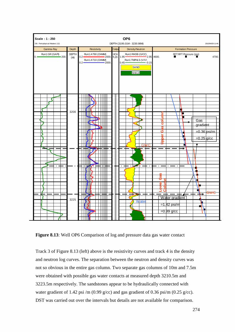
274


Track 3 of Figure 8.13 (left) above is the resistivity curves and track 4 is the density

and neutron log curves. The separation between the neutron and density curves was

not so obvious in the entire gas column. Two separate gas columns of 10m and 7.5m

were obtained with possible gas water contacts at measured depth 3210.5m and

3223.5m respectively. The sandstones appear to be hydraulically connected with

water gradient of 1.42 psi /m (0.99 g/cc) and gas gradient of 0.36 psi/m (0.25 g/cc).

DST was carried out over the intervals but details are not available for comparison.

OP6Scale : 1 : 250


Gamma-Ray


Depth

DEPTH

(M)

Resistivity

Run1:AT90 (OHMM)0.2 2000.

Run1:AT10 (OHMM)0.2 2000.

Caliper

HCA6.16.

Density/Neutron

Run1:RHOB (G/CC)1.95 2.95

Run1:TNPHLS (V/V)0.45 -0.15

SAND

SHALE

Formation Pressure

RFT:RFT Pressure (psi)4600. 4700.

3200

3225

GWC

GWC

Up

per

Gas

co

lum

nL

ow

er

Gas

Co

lum

n

Water

Gas

gradient

=0.36 psi/m

=0.25 g/cc

Water gradient

=1.42 psi/m

=0.99 g/cc

275

However, the resistivity curve indicated a gas water contact at 3223.5m which almost

coincide with that determined from the pressure data.

Figure 8.14 is the gas water contact comparison for well MA2 presented below.

Figure 8.14: Well MA 2 comparison of log and pressure data gas water contact

Presented in Figure 8.15 below is the comparison of well MA3 log and pressure data

determined gas water contact.

MA2Scale : 1 : 240


Gamma-Ray

RUn2:GR (GAPI)0. 200.

Depth

DEPTH

(M)

Resistivity

RUn2:HLLD (OHMM)0.2 2000.

RUn2:HLLS (OHMM)0.2 2000.

Density/Neutron

RHOBE (gm/cc)1.95 2.95

RUn2:NPHI (V/V)0.45 -0.15

Formation Pressure

RFT:Pressure ()4350. 4420.

2975

2955

2965

Possible GWCG

as c

olum

n

Water

Gas gradient

=0.35 psi/m

=0.24 g/cc

Water gradient

=1.4 8psi/m

=1.04 g/cc

Pressure (psi)

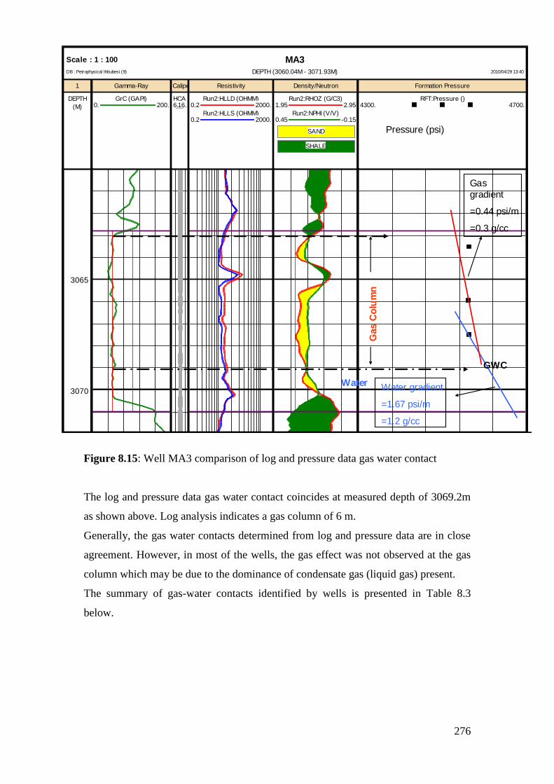
276

Figure 8.15: Well MA3 comparison of log and pressure data gas water contact

The log and pressure data gas water contact coincides at measured depth of 3069.2m

as shown above. Log analysis indicates a gas column of 6 m.

Generally, the gas water contacts determined from log and pressure data are in close

agreement. However, in most of the wells, the gas effect was not observed at the gas

column which may be due to the dominance of condensate gas (liquid gas) present.

The summary of gas-water contacts identified by wells is presented in Table 8.3

below.

MA3Scale : 1 : 100


1

DEPTH

(M)

Gamma-Ray

GrC (GAPI)0. 200.

Caliper

HCA6.16.

Resistivity

Run2:HLLD (OHMM)0.2 2000.

Run2:HLLS (OHMM)0.2 2000.

Density/Neutron

Run2:RHOZ (G/C3)1.95 2.95

Run2:NPHI (V/V)0.45 -0.15

SAND

SHALE

Formation Pressure

RFT:Pressure ()4300. 4700.

3065

3070

GWCG

as C

olu

mn

WaterWater gradient

=1.67 psi/m

=1.2 g/cc

Gas

gradient

=0.44 psi/m

=0.3 g/cc

Pressure (psi)

277

Table 8.3: Summary of gas water contact

Well Name Interval (m) Gas Water Contact(GWC)

(m)

OP1 3368-3375 3374.0

OP3 3275-3287 3284.0

3354-3370 3364.0

OP4 3238-3258 3255.0

OP6 3197-3213 3210.5

3213-3227 3223.5

MA2 2955-2967 2964.0

MA3 3063-3070 3069.0

278

CHAPTER NINE

APPLICATION OF RESULTS, DETERMINATION OF CUT-OFF

AND NET PAY

9.1 INTRODUCTION

One of the major challenges with determination of petrophysical properties from core,

wireline logs, and production test is that, data sources measure different physical

parameters and represent different sample volumes. Sampling bias also contribute to

the challenges. According to Lovell et al (1998), measurements of petrophysical

properties in the laboratory or down-hole device would under favourable conditions

and experimental experience, produce an accurate measure of the parameter the

device was designed to measure. The wireline tools do not record petrophysical

properties directly but have to be interpreted (chapter 2), and the degree to which the

interpreted values are accurate is difficult to ascertain. To minimize the uncertainty or

error associated wireline data, core data was used to calibrate wireline log

measurements (chapter 6) in order to obtain accurate measurements.

The methods used to give a better and more reliable estimate of petrophysical

properties were based on core data (sedimentological description and petrophysical)

which helps in identification of lithofacies, petrofacies and flow zone indicators. Well

test effective permeability estimates were available for well OP2 (chapter 7) and a

good match with wireline log prediction of permeability using the Morris Biggs gas

model was obtained. The absolute permeability (K) was obtained predicted from the

porosity estimate using a regression equation established at the core plug scale in

chapter 5. Though the expression obtained relating linear porosity to the logarithm of

permeability at the core plug scale is not likely the same at the wireline scale. As

indicated in chapter 5, diagenesis is present in the studied intervals and as such will

influence some of the wireline log measurements. The core plug porosities were

corrected for overburden effects and the core permeability for gas effect

(Klinkenberg) in order to obtain results close to in situ measurements.

According to Elfenbein et al (2003) and Zhang et al (2004), wells test results when

carefully calibrated, actually reproduce in situ measurement results. There exist many

279

published methods to estimate petrophysical properties from well data. Some of these

have been discussed in the previous chapters. This section of the study focused on the

estimate of basic petrophysical properties (volume of shale, porosity, permeability and

water saturation) in non-cored wells.

9.2 Determination of Petrophysical Properties in Non-Cored Wells.

The petrophysical models of volume of shale, porosity and water saturation derived

from the three cored wells (OP1, OP2 and OP3) was applied to non-cored wells as

presented in some of the wells below.

The estimation of volume of clay in non-cored wells was based on the Steiber volume

of shale correction equation which showed very good agreement with the whole rock

mineralogy core data as shown in Figures 6.3 and 6.4 of chapter 6.

The equation 6.13 of chapter 6 was applied to non-cored wells in order to estimate

overburden porosities using the sonic porosity log that best correlated with the core

porosity data. The sonic porosity log was run in all the wells so it was easier to use it

in estimation of the overburden porosity.

The capillary pressure water saturation was used to calibrate log calculated water

saturations as discussed in section 6.3 (chapter 6). The Simandoux and Wax-man

Smith models best matched with capillary pressure estimated water saturations and

hence will was used to estimate water saturations in non-cored wells.

Presented in the Figures below are the results obtained from the application of

petrophysical obtained models from core to non-cored wells and intervals.

The Gamma-Ray is represented in track3, porosity (total and effective in track 4),

water saturation (Sw) in track 5, Permeability (Absolute k and effective) in track 6,

and volume of clay (track 7) in the graphics presented below.

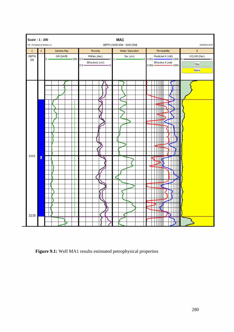
280

Figure 9.1: Well MA1 results estimated petrophysical properties

MA1Scale : 1 : 200


1

DEPTH

(M)

2 Gamma-Ray

GR (GAPI)0. 200.

Porosity

PhiDen (dec)0.5 0.

Effective1 (v/v)0.5 0.

Water Saturation

Sw (v/v)1. 0.

Permeability


Effective K (md)0.001 1000.

9

VCLGR (Dec)0. 1.

Clay

Matrix

32251

3235

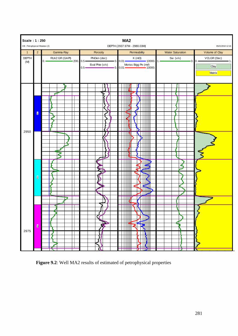
281

Figure 9.2: Well MA2 results of estimated of petrophysical properties

MA2Scale : 1 : 250


1

DEPTH

(M)

2 Gamma-Ray

RUn2:GR (GAPI)0. 200.

Porosity

PhiDen (dec)0.5 0.

Eval Phie (v/v)0.5 0.

Permeability

K (mD)0.01 10000.

Moriss Bigg Pe (md)0.01 10000.

Water Saturation

Sw (v/v)1. 0.

Volume of Clay

VCLGR (Dec)0. 1.

Clay

Matrix

2950

2975

1

2

3

282

Figure 9.3: Well MA3 results of estimated petrophysical properties

MA3Scale : 1 : 250


1

DEPTH

(M)

2 Gamma-Ray


Porosity

PhiDen (dec)0.5 0.

Effective Poro (v/v)0.5 0.

Water Saturation

SW (v/v)0. 1.

Permeability

K (mD)0.001 1000.

Effective K (md)0.001 1000.

9

VCLGR (Dec)0. 1.

Clay

Matrix

3075

1

2

3085

283

Figure 9.4: Well MA4 results of estimated petrophysical properties

MA4Scale : 1 : 400

DEPTH (3149.04M - 3162.M) 2010/05/21 16:53DB : Petrophysical Ihbubesi (10)

1

DEPTH

(M)

2 Gamma-Ray

GrC (GAPI)0. 200.

Porosity

PhiDen (dec)0.5 0.


Water Saturation

Sw (v/v)0. 1.

Permeability

K (mD)0.001 1000.

Effective Perm (md)0.001 1000.

9

VCLGR (Dec)0. 1.

Clay

Matrix

3150

1

MA4Scale : 1 : 400


3300

2

MA4Scale : 1 : 400


3350

3

284

Figure 9.5: Well OP4 results of estimated petrophysical properties

OP4Scale : 1 : 300


1

DEPTH

(M)

2 3

GrC (GAPI)0. 200.

4

PhiDen (dec)0.5 0.


5

Sw (v/v) (v/v)0. 1.

6

K (mD)0.001 1000.

Perm (md)0.001 1000.

9

VCLGR (Dec)0. 1.

Clay

Matrix

1

OP4Scale : 1 : 300


3250

2

285


OP5Scale : 1 : 150


1

DEPTH

(M)

2 3


4

PhiDen (dec)0.5 0.

Phie Eval1 (v/v)0.5 0.

5

Sw eval (v/v)0. 1.

6

K (mD)0.001 1000.

Effect Perm (md)0.001 1000.

7

VCLGR (Dec)0. 1.

Clay

Matrix

1

OP5Scale : 1 : 150


33252

3330

3207

3210

286


OP6Scale : 1 : 500


1

DEPTH

(M)

2 3


4

PhiDen (Dec)0.5 0.


5

Sw (v/v) (v/v)0. 1.

6

K (mD)0.001 1000.

Effect Perm (md)0.001 1000.

7

VCLGR (Dec)0. 1.

Clay

Matrix

3200

1

OP6Scale : 1 : 500


2

3

OP6Scale : 1 : 500


4

287

9.3 CUT-OFF DETERMINATION

The cut-off concept is aimed at defining the effective petrophysical properties of a

given geological unit in the presence of poor reservoir zones. In order to assess the

efficiency of reservoir recovery mechanisms, the initial hydrocarbon volume must

relate to reservoir rock. Where it does not, the hydrocarbon will have little chance of

being, they may not contribute to reservoir dynamics and they should not be included

within the accumulation volume against which recovery is to be assessed

(Worthington, 2008).

The starting point in determining cut-off is to identify reference parameter that allows

us to distinguish between intervals that have reservoir potential and intervals that do

not. There is no single universally applicable approach to the identification of cut-off

(Worthington & Cosentino, 2005). One of the most important steps is to establish the

linkage between a conventional core measurement and a reference parameter that

distinguishes between reservoir and non-reservoir rock. The evaluation of

hydrocarbon volumes requires cut-offs so that net reservoir intervals (net pay) that

contain sufficient hydrocarbon potentials and allow adequate hydrocarbon flow can be

identified.

The net pay is defined on flow rate criteria and the fluids produce. Rocks with

sufficient permeability to flow fluids at commercially significant rates are classified as

net sandstone or net reservoir. If they produce hydrocarbons at a commercially

acceptable hydrocarbon/water ratio, they are classified as net pay (Suzanne & Robert,

2004).

A non reservoir rock may have porosity and permeability that is too low and zero

hydrocarbon saturation. The major control is often the lithology. Though shales are

classified as non reservoir rocks, they often contain hydrocarbon with high saturations

but have porosity and permeability that are too low for the hydrocarbon to be

extracted. Sandstones on the contrary could be considered as reservoir rocks provided

that they contain sufficiently high hydrocarbon could be extracted without

difficulties..

The permeability cut-off is very often considered as the controlling parameter in net

pay since it is dependent on a limited number of parameters including the fluid

mobility, viscosity; pressure differential and reservoir drive mechanism. A common

arbitrary approach of determining permeability cut-off is to set permeability cut-off

288

for gas reservoir net pay at 0.1mD and oil reservoir net pay at 1.0 mD. This approach

is arbitrary since it does not take into consideration the reservoir fluid characteristics

(George & Stiles, 1978).

To separate pay from non-pay, this study used the combined plot of porosity-

permeability for the cored wells in the field in conjunction with the classified facies

and log derived volume of shale and water saturation cut-offs. Also, petrofacies and

flow zone indicators identified in the previous chapter was also used to identify rocks

in pay and non-pay intervals.

9.3.1 Porosity Cut-Off Determination

To discriminate between reservoir and non-reservoir, each data had to meet a porosity

cut-off. The cross plot of conventional core porosity-permeability data corrected to

equivalent in situ conditions in wells with facies plot was used to define a porosity

equivalent to a minimum permeability considered capable of flowing hydrocarbon.

The Figure 9.8a below presents the porosity-permeability cross plot for the combined

wells with core porosity and permeability data used for cut-off determination.

Figure 9.8a: Multi-Well porosity-permeability plot for cut-off determination

Multi-Well

Porosity -Permeability and Facies Plot

0. 0.06 0.12 0.18 0.24 0.3

Core Porosity (v/v)

0.001

0.01

0.1

1.

10.

100.

1000.

10000.

Co

re P

erm

eab

ilit

y (

mD

)

A6

A5

A4

A3

A2

A1

0.

6.

Facies

-

R2= 0.9201 Well

OP1

OP2

OP3

A5 & A6

A1 &A2

A3 & A4

Φc

K c

Non-Reservoir

Region

Net

Reservoir

Region

289

The porosity-permeability relationship indicated a conventional core Klinkenberg

corrected permeability of approximately 0.1mD corresponding to an approximate

overburden corrected porosity of 10 percent as cut-off points for reservoir and non

reservoir regions. The points Kc and Φc on y and x axis on the plot are the

permeability and porosity cut-off points respectively.

Facies A6 dominates the non reservoir region with facies A5 insignificantly

distributed in this region. This confirms that facies A6 is a non reservoir rock. The

histogram of the frequency distribution of permeability and porosity showing the cut-

off points are presented in Figure 9.8b below.

Figure 9.8b: Multi-Well permeability and porosity histogram distributions

The obtained permeability and porosity cut-off criteria were also applied to

petrofacies in order to determine petrofacies that meet up the cut-off criteria. The plot

indicated a cut-off point on micro-petrofacies. That is, for a rock to be classified as

reservoir rock, it must have a pore throat radius of at least 0.2 microns.

Multi-Well Interval histogram


0

20

40

60

80

100

Cu

mu

lativ

e F

req

uen

cy

0.001 0.01 0.1 1. 10. 100. 1000. 10000.0

2

4

6

Nu

mb

er

of

Po

ints

Curve WellCore Klinkenberg OP1Core Klinkenberg OP2Core Klinkenberg OP3

Core Porosity Histogram Plot

Multi-well Interval histogram

0

20

40

60

80

100

Cu

mu

lativ

e F

req

uen

cy

0. 0.3

0

2

4

6

Nu

mb

er

of

Po

ints

Curve WellCore Porosity OP3Core Porosity OP2Core Porosity OP1

Reservoir

Cut-Off

Permeability

0.1mD

Non

Reservoir

0.180.06 0.12 0.24

Reservoir

Non

Reservoir

Porosity

Cut-Off 10%

290

The Nano rock type was identified as a non-reservoir rock because it failed to meet

the cut-off criteria. The plot is presented in Figure 9.8c below.

Figure 9.8c: Application of permeability and porosity cut-off to petrofacies

9.3.2 Volume of Shale Cut-Off Determination

The volume shale cut-off is used to discriminate between reservoir and non reservoir

rock by allowing all rocks volume of shale equal to or less than certain value of the

total reservoir volume.

The multi-well volume of shale versus porosity and gamma-ray log used to determine

the volume of shale cut-off is presented in Figure 9.9a below.

Multi-Well


0. 0.06 0.12 0.18 0.24 0.3

Porosity (v/v)

0.001

0.01

0.1

1.

10.

100.

1000.

10000.

Permeability (mD)

Nanno

Micro

Meso

Macro

Mega

0.01

30.

Rock Type (microns)

Multi-Well


0. 0.06 0.12 0.18 0.24 0.3

Porosity (v/v)

0.001

0.01

0.1

1.

10.

100.

1000.

10000.

Permeability (mD)

Nanno

Micro

Meso

Macro

Mega

0.01

30.

Rock Type (microns)

Kc

? C

Reservoir

Non-Reservoir

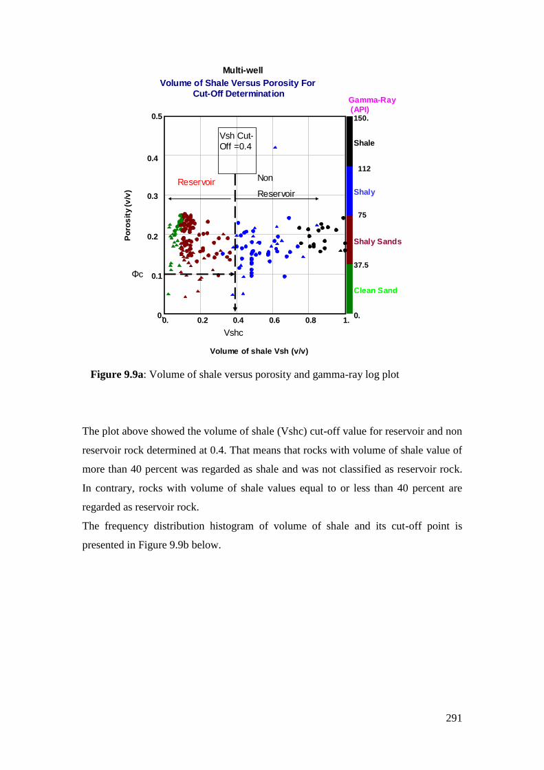
291

Figure 9.9a: Volume of shale versus porosity and gamma-ray log plot

The plot above showed the volume of shale (Vshc) cut-off value for reservoir and non

reservoir rock determined at 0.4. That means that rocks with volume of shale value of

more than 40 percent was regarded as shale and was not classified as reservoir rock.

In contrary, rocks with volume of shale values equal to or less than 40 percent are

regarded as reservoir rock.

The frequency distribution histogram of volume of shale and its cut-off point is

presented in Figure 9.9b below.

Multi-well

Volume of Shale Versus Porosity For

Cut-Off Determination

0. 0.2 0.4 0.6 0.8 1.

Volume of shale Vsh (v/v)

0.

0.1

0.2

0.3

0.4

0.5

Po

ros

ity

(v/v

)

Clean Sand

Shaly Sands

Shaly

Shale

0.

150.

Gamma-Ray

(API)

37.5

75

112

Vsh Cut-

Off =0.4

Non

Reservoir

Reservoir

Φc

Vshc

292

Figure 9.9b: Multi-Well vclay frequency distribution and cut-off point

9.3.3 Water Saturation Cut-Off Determination.

The water saturation cut-off discriminates between hydrocarbon bearing sandstones

(pay) and intervals and water (wet) bearing intervals. Intervals that have water

saturation greater than 65 percent water saturation were assumed to be wet or non-

productive intervals.

Presented in Figure 9.10 below are the water saturation versus porosity cross plot and

the water saturation frequency distribution histogram plot.

Multi-Well

Volume of shale frequency Distribution

0

20

40

60

80

100

Cum

ulative Frequency

0. 1.0

10

20

30

40

50

perc

enta

ge

Curve Well

OP1

OP2

OP3

VClay (v/v)

0.80.60.40.2

0.4 Vclay cut-off

293

Figure 9.10: Multi-Well porosity vs water saturation and frequency distribution

9.4 Determination of Net Pay

The gross is regarded as the thickness of the reservoir interval that contains zones of

which hydrocarbon can be produced and zones which does not favour the production

of hydrocarbon. Net pay is any interval within the reservoir that contains producible

hydrocarbon at economic rate given a specific production method. It represents the

portion of the reservoir that contains high storability and mobility and significant

hydrocarbon saturation.

Net pay is used to compute volumetric hydrocarbon in place and to determine the total

energy of the reservoir which are both moveable and non-moveable hydrocarbons.

Other use of net pay is to evaluate the potential amount of hydrocarbon available for

secondary recovery (Cobb & Marek, 1998).

The distinction between gross and net pay is made by applying cut-off values in the

petrophysical analysis. In this study, cut-off values of porosity (≥ 0.1), volume of

shale (≤ 0.4) and water saturation (≤ 0.65) were used to identify pay intervals. That is,

Multi-Well

Porosity Versus Water Saturation

0. 0.1 0.2 0.3 0.4 0.5

Porosity (v/v)

0.1

0.2

0.5

1.

Wa

ter S

atu

ra

tio

n (

v/v

)

Swc

Productive intervals

Wet intervals

Multi-Well

Water Saturation Frequency Distribution

0

20

40

60

80

100

Cu

mu

lativ

e F

req

uen

cy

0. 1.0

2

4

Perc

en

t o

f T

ota

l

Curve Well

OP1

OP2

OP3

0.80.60.40.2


Productive intervalwet

Swc

294

intervals with porosity equal to and greater than 10 percent and volume of shale less

than or equal to 40 percent and water saturation less than or equal to 65 percent were

regarded as net pay intervals. Capillary pressure and relative permeability data

support this 65 % pay cut-off.

The net to gross ratio is the thickness of net sand divided by the thickness of gross

sand. This ratio is often used to represent the quality of a reservoir zone and for

volumetric hydrocarbon calculations.

Using the cut-off limits, flag curves were created in the database for net reservoir

interval (red colour) and gross reservoir (green). The net to gross ratio determined

could be used to calculate the volume of gas originally in place. However, the

calculation of volume of hydrocarbon is not part of the scope of this study.

Presented in Table 9.1 to 9.8 below are the calculated net pay summary for wells with

the corresponding graphics in Figure 9.11 to 9.20.

Table 9.1: Summary of calculated reservoir pay parameters for Well OP1

Zone Name Top Bottom Gross Net N/G Av Phi Av Sw Av Vcl

(m) (m) (m) (m) (v/v) (v/v) (v/v)

Reservoir 1 3303 3330.9 27.9 0 0 --- --- ---

Reservoir 2 3368 3376.3 8.3 6.29 0.758 0.153 0.521 0.284

Reservoir 3 3390.5 3416 25.5 0 0 --- --- ---

Three reservoirs were encountered in well OP1 of which one proved to have net pay

(6.29m) having average porosity of 15.3 %, water saturation of 52 % and 28 %

volume of shale as presented in Table 9.1 above and Figure 9.11 below.

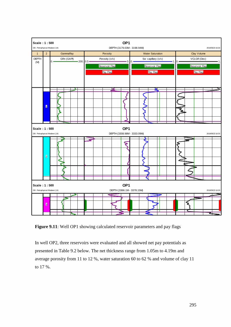
295

Figure 9.8: Well OP1 showing Net Pay Flag

Table 9.2: Well OP2 Summary of calculated Reservoir Pay Parameters


(m) (m) (m) (m) (v/v) (v/v) (v/v)

14Ct1 3184.4 3203.1 18.7 4.19 0.224 0.113 0.614 0.17

14Dt1 3308 3320.7 12.7 1.05 0.083 0.11 0.608 0.11

14Et1 3446 3468.2 22.2 1.05 0.047 0.12 0.619 0.13

All Zones 3184.4 3468.2 53.6 6.29 0.117 0.114 0.613 0.153

Figure

Figure 9.11: Well OP1 showing calculated reservoir parameters and pay flags

In well OP2, three reservoirs were evaluated and all showed net pay potentials as

presented in Table 9.2 below. The net thickness range from 1.05m to 4.19m and

average porosity from 11 to 12 %, water saturation 60 to 62 % and volume of clay 11

to 17 %.

OP1Scale : 1 : 500


1

DEPTH

(M)

2 GammaRay

GRn (GAPI)0. 200.

Porosity

Porosity (v/v)0.5 0.

Reservoir Flag

Pay Flag

Water Saturation

Sw capillary (v/v)0. 1.

Reservoir Flag

Pay Flag

Clay Volume

VCLGR (Dec)0. 1.

Reservoir Flag

Pay Flag

1

OP1Scale : 1 : 500


2

OP1Scale : 1 : 500


3

296

Table 9.2: Summary of calculated reservoir pay parameters for well OP2


(m) (m) (m) (m) (v/v) (v/v) (v/v)

14Ct1 3184.4 3203.1 18.7 4.19 0.224 0.113 0.614 0.17

14Dt1 3308.0 3320.7 12.7 1.05 0.083 0.11 0.608 0.11

14Et1 3446.0 3468.2 22.2 1.05 0.047 0.12 0.619 0.13

All Zones 3184.4 3468.2 53.6 6.29 0.117 0.114 0.613 0.153

OP2Scale : 1 : 500


1

DEPTH

(M)

2 GammaRay

GRn (GAPI)0. 200.

Porosity

EFFect (v/v)0.5 0.

Reservoir Flag

Pay Flag

Water Saturation

Sw (dec) (v/v)0. 1.

Reservoir Flag

Pay Flag

Clay Volume

VCLGR (Dec)0. 1.

Reservoir Flag

Pay Flag

3200

1

OP2Scale : 1 : 500


2

OP2Scale : 1 : 500


3450

3

Figure 9.13: Well OP2 showing calculated reservoir parameters and pay flag

297

In well OP3, the gross thickness range from 9.1 to 16.9 m and net thickness from 2.33

to 13.33 m. An average porosity of 15.7 %, water saturation of 53% and volume of

clay of 7 % were calculated as presented in Table 9.3 and Figure 9.14 below.



(m) (m) (m) (m) (v/v) (v/v) (v/v)

14Jt1 3230.1 3239.2 9.1 5.96 0.655 0.143 0.5 0.055

14Et1 3276.4 3286.3 9.9 5.24 0.529 0.161 0.544 0.084

14Et1 3310.1 3317.1 7 2.33 0.333 0.158 0.526 0.055

14Bt1 3354.1 3371 16.9 13.23 0.783 0.161 0.545 0.066

All Zones 3230.1 3371 42.9 26.76 0.624 0.157 0.534 0.066

Figure 9.14: Well OP3 graphics of calculated reservoir parameters and flags

OP3Scale : 1 : 500


1

DEPTH

(M)

2 GammaRay

GRn (GAPI)0. 200.

Porosity

Effect (v/v)0.5 0.

Reservoir Flag

Pay Flag

Water Saturation

Sw (v/v) (v/v)0. 1.

Reservoir Flag

Pay Flag

Clay Volume

VCLGR (Dec)0. 1.

Reservoir Flag

Pay Flag

1

OP3Scale : 1 : 500


2

OP3Scale : 1 : 500


3

OP3Scale : 1 : 500


4

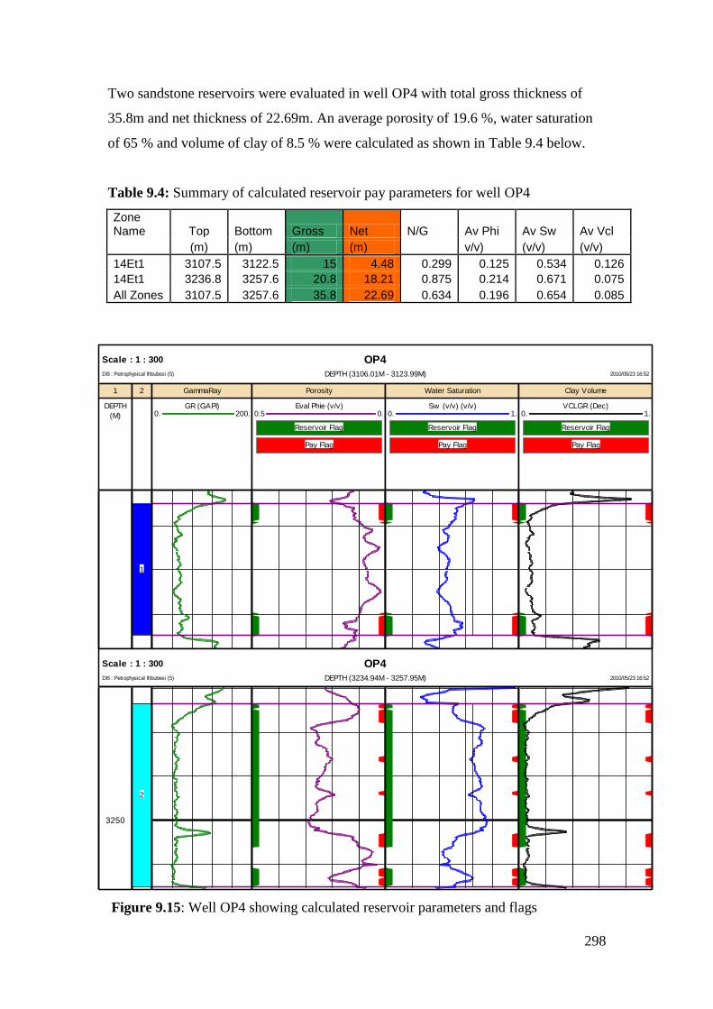
298

Two sandstone reservoirs were evaluated in well OP4 with total gross thickness of

35.8m and net thickness of 22.69m. An average porosity of 19.6 %, water saturation

of 65 % and volume of clay of 8.5 % were calculated as shown in Table 9.4 below.



(m) (m) (m) (m) v/v) (v/v) (v/v)

14Et1 3107.5 3122.5 15 4.48 0.299 0.125 0.534 0.126

14Et1 3236.8 3257.6 20.8 18.21 0.875 0.214 0.671 0.075

All Zones 3107.5 3257.6 35.8 22.69 0.634 0.196 0.654 0.085

Figure 9.15: Well OP4 showing calculated reservoir parameters and flags

OP4Scale : 1 : 300


1

DEPTH

(M)

2 GammaRay

GR (GAPI)0. 200.

Porosity


Reservoir Flag

Pay Flag

Water Saturation

Sw (v/v) (v/v)0. 1.

Reservoir Flag

Pay Flag

Clay Volume

VCLGR (Dec)0. 1.

Reservoir Flag

Pay Flag

1

OP4Scale : 1 : 300


3250

2

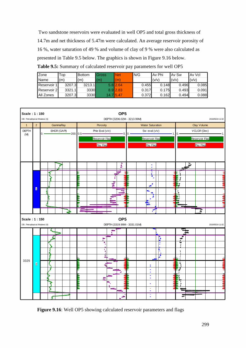
299

Two sandstone reservoirs were evaluated in well OP5 and total gross thickness of

14.7m and net thickness of 5.47m were calculated. An average reservoir porosity of

16 %, water saturation of 49 % and volume of clay of 9 % were also calculated as

presented in Table 9.5 below. The graphics is shown in Figure 9.16 below.



Zone Top Bottom Gross Net N/G Av Phi Av Sw Av Vcl Name (m) (m) (m) (m) (v/v) (v/v) (v/v) Reservoir 1 3207.3 3213.1 5.8 2.64 0.455 0.148 0.496 0.085 Reservoir 2 3321.1 3330 8.9 2.83 0.317 0.175 0.493 0.091 All Zones 3207.3 3330 14.7 5.47 0.372 0.162 0.494 0.088

OP5Scale : 1 : 150


1

DEPTH

(M)

2 GammaRay

EHGR (GAPI)0. 200.

Porosity

Phie Eval (v/v)0.5 0.

Reservoir Flag

Pay Flag

Water Saturation

Sw eval (v/v)0. 1.

Reservoir Flag

Pay Flag

Clay Volume

VCLGR (Dec)0. 1.

Reservoir Flag

Pay Flag

1

OP5Scale : 1 : 150


33252

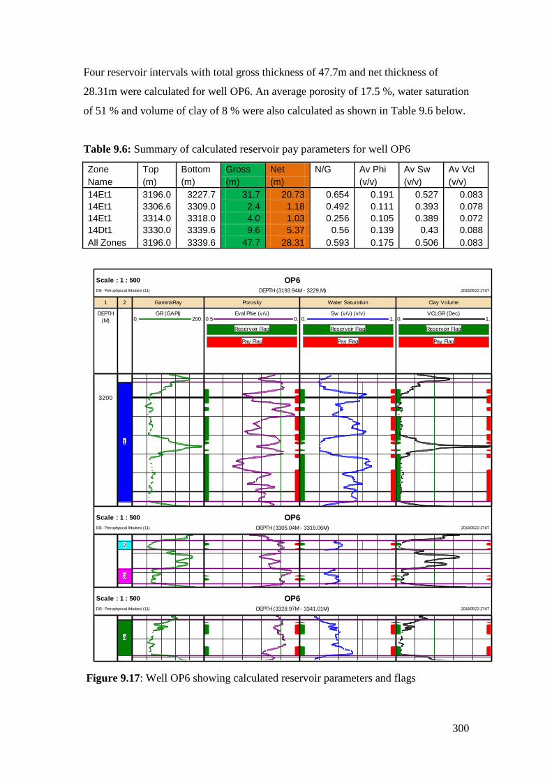
300

Four reservoir intervals with total gross thickness of 47.7m and net thickness of

28.31m were calculated for well OP6. An average porosity of 17.5 %, water saturation

of 51 % and volume of clay of 8 % were also calculated as shown in Table 9.6 below.


Zone Top Bottom Gross Net N/G Av Phi Av Sw Av Vcl

Name (m) (m) (m) (m) (v/v) (v/v) (v/v)

14Et1 3196.0 3227.7 31.7 20.73 0.654 0.191 0.527 0.083

14Et1 3306.6 3309.0 2.4 1.18 0.492 0.111 0.393 0.078

14Et1 3314.0 3318.0 4.0 1.03 0.256 0.105 0.389 0.072

14Dt1 3330.0 3339.6 9.6 5.37 0.56 0.139 0.43 0.088

All Zones 3196.0 3339.6 47.7 28.31 0.593 0.175 0.506 0.083


OP6Scale : 1 : 500


1

DEPTH

(M)

2 GammaRay

GR (GAPI)0. 200.

Porosity


Reservoir Flag

Pay Flag

Water Saturation

Sw (v/v) (v/v)0. 1.

Reservoir Flag

Pay Flag

Clay Volume

VCLGR (Dec)0. 1.

Reservoir Flag

Pay Flag

3200

1

OP6Scale : 1 : 500


2

3

OP6Scale : 1 : 500


4

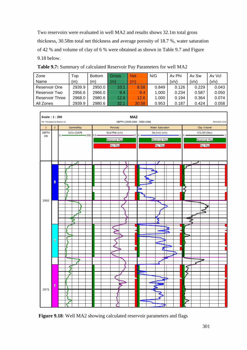
301

Two reservoirs were evaluated in well MA2 and results shows 32.1m total gross

thickness, 30.58m total net thickness and average porosity of 18.7 %, water saturation

of 42 % and volume of clay of 6 % were obtained as shown in Table 9.7 and Figure

9.18 below.

Table 9.7: Summary of calculated Reservoir Pay Parameters for well MA2


Name (m) (m) (m) (m) (v/v) (v/v) (v/v)

Reservoir One 2939.9 2950.0 10.1 8.58 0.849 0.126 0.229 0.043

Reservoir Two 2956.6 2966.0 9.4 9.4 1.000 0.234 0.587 0.050

Reservoir Three 2968.0 2980.6 12.6 12.6 1.000 0.194 0.364 0.074

All Zones 2939.9 2980.6 32.1 30.58 0.953 0.187 0.424 0.058

Figure 9.18: Well MA2 showing calculated reservoir parameters and flags

MA2Scale : 1 : 250


1

DEPTH

(M)

2 GammaRay

GrCn (GAPI)0. 200.

Porosity


Reservoir Flag

Pay Flag

Water Saturation

Sw (v/v) (v/v)0. 1.

Reservoir Flag

Pay Flag

Clay Volume

VCLGR (Dec)0. 1.

Reservoir Flag

Pay Flag

2950

2975

1

2

3

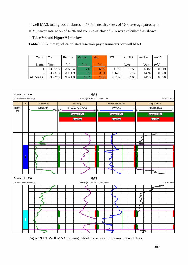
302

In well MA3, total gross thickness of 13.7m, net thickness of 10.8, average porosity of

16 %; water saturation of 42 % and volume of clay of 3 % were calculated as shown

in Table 9.8 and Figure 9.19 below.

Table 9.8: Summary of calculated reservoir pay parameters for well MA3


Name ((m) (m) (m) (m)

(v/v) (v/v) (v/v)

1 3062.8 3070.4 7.6 6.99 0.92 0.159 0.382 0.019

2 3085.8 3091.9 6.1 3.81 0.625 0.17 0.474 0.038

All Zones 3062.8 3091.9 13.7 10.8 0.789 0.163 0.416 0.026

Figure 9.19: Well MA3 showing calculated reservoir parameters and flags

MA3Scale : 1 : 240


1

DEPTH

(M)

2 GammaRay

GrC (GAPI)0. 200.

Porosity

Effective Poro (v/v)0.5 0.

Reservoir Flag

Pay Flag

Water Saturation

SW (v/v)0. 1.

Reservoir Flag

Pay Flag

Clay Volume

VCLGR (Dec)0. 1.

Reservoir Flag

Pay Flag

1

MA3Scale : 1 : 240


2

303

Total gross thickness of 46.1m; net thickness of 36.25m; average porosity of 18.9 %;

water saturation of 59 %, and volume of clay of 15% were calculated for well MA4 as

shown in Table 9.9 and Figure 9.20 below.

Table 9.9: Summary of calculated reservoir pay parameters for well MA4


(m) (m) (m) (m) (v/v) (v/v) (v/v)

1 3150.6 3161 10.4 8.53 0.821 0.19 0.584 0.114

2 3293 3301 8 5.16 0.646 0.16 0.528 0.184

3 3332.1 3359.8 27.7 22.56 0.814 0.196 0.602 0.162

All Zones 3150.6 3359.8 46.1 36.25 0.786 0.189 0.589 0.154

Figure 9.20: Well MA4 graphics of calculated reservoir parameters and flags

MA4Scale : 1 : 400


1

DEPTH

(M)

2 GammaRay

GrC (GAPI)0. 200.

Porosity


Reservoir Flag

Pay Flag

Water Saturation

Sw (v/v)0. 1.

Reservoir Flag

Pay Flag

Clay Volume

VCLGR (Dec)0. 1.

Reservoir Flag

Pay Flag

3150

1

MA4Scale : 1 : 400


3300

2

MA4Scale : 1 : 400


3350

3

304

CHAPTER TEN

CONCLUSIONS AND RECOMMENDATIONS

The Petrophysical evaluation of Albian age gas bearing sandstone reservoirs of the O-

M Field, offshore South Africa has been carried out. It is hoped that this thesis will

serve as a guide for future studies on petrophysical evaluations. Due to the complex

nature of the O-M field, the petrophysical evaluation approach was chosen to assess

the reservoirs within the Albian age formation. In total, ten wells were drilled within

the field, and eight of these made gas discoveries with only two being wet. The study

was divided into two sections which are the basic concepts (Chapter 1 to 3) and

petrophysical evaluations (Chapters 4 to 9). A brief summary of the chapters studied

and recommendations for further work are presented below.

Chapter one gives the general introduction and outline to the study. The Albian age

gas bearing reservoir sandstones evaluated range between 2800m to 3500m depending

on the position of the well. The studied area is zoned into two, the MA zone in the

Northern part of the field and the OP zone in the central and Southern part of the field.

The reservoirs in the area are in a sequence of fluvial channel sands of Albian to

Cenomanian age. The area is predominantly gas prone with gas being sourced from

Pre-Hautervarian Lacustrine shales in rift phase half graben sub-basins and

terrigeneous derived type II kerogen from upper Cretaceous drift sequence. The

channels are meandering systems.

Chapter two focused on the principles and uses of wireline logs. The wireline logs

were grouped into active and passive tools. The active tools measure the response of

formation to some form of excitations. This includes the density, neutron, resistivity

and nuclear magnetic resonance tools. The passive tools measure natural occurring

phenomena such as gamma radiation that is emitted by elements in the rock or electric

potential caused by differences in salinity of the mud in the Well and formation water.

Examples are the gamma-ray and spontaneous potential logs.

Chapter three gives the description of fundamental petrophysical properties which

includes the porosity, permeability and water saturation. The main petrophysical

305

properties are porosity, permeability, and saturation. Porosity determines the storage

capacity for hydrocarbon and permeability determines the fluid flow capacity of the

rock. Saturation is the fraction of the pore spaces that is occupied by hydrocarbon or

water. Accurate determination of these petrophysical properties is essential to assess

the economic viability of the development of reservoirs.

The petrophysical evaluation section starts with wireline log editing and

normalization in chapter four. When raw log data are collected for formation

evaluation purposes, it is essential to check the quality of the data and perform editing

if necessary before using it for qualitative interpretations. Log editing is a form of log

interpretation aimed at removing problems that affect log readings and provide the

best possible presentation of the in situ properties measured. Some of the problems

encountered in the study and were corrected includes depth matching, environmental

corrections, noise removal and curve matching of different RUNs into a continuous

curve. After performing the editing processes, curves were normalized. Curve

normalization is a mathematical process that adjusts for differences among data from

varying sources in order to create a common basis for comparison.

Chapter five is the rate determining step of this research. It discussed the ground truth

of conventional and special core analysis results of the key wells (OP1, OP2 and OP3)

which was essential for calibration of non-cored wells. The approach adopted by

Nieto Rojas (1998) for grouping lithofacies was used and six rock units (facies A1,

A2, A3, A4, A5 and A6) were grouped according to textural and structural features

and grain sizes. Facies A1, A2, A3, A4 and A5 were classified were classified as

reservoir rocks in terms of their porosity and permeability and they showed good

reservoir quality while facies A6 was regarded as no reservoir rock. The grain density

value for wells showed a range of 2.58 g/cc to 2.72 g/cc with a mean grain density of

2.67 g/cc obtained from the histogram analysis which was used for other evaluations.

Core porosity ranged from 1 % to 24.4 % with an average of 13.5 %. The low

porosity values were recorded in intervals of clay/siltstones and the high porosity

values were associated with clean sandstone intervals. Core permeability ranged from

0.006mD to 1095mD with a mean value of 10mD.

306

Three types of fluid saturation were obtained from core analysis of well OP1 and

OP3. An average water saturation of 57 %, gas saturation of 38 % and oil saturation

of 5 % was measured in well OP1. Two cores were taken in well OP3 with core 1

showing 62 % of gas saturation and 38 % of water saturation. Core 2 of the same well

showed 65 % of water saturation and 35 % of gas saturation. The conventional core

porosity measured at room conditions were converted to net effective overburden

stress at in situ reservoir conditions (4830 psi). The cementation exponent (m) of 1.94

and saturation exponent (n) of 1.8 were determined from special core analysis

measurements. The petrography study of thin section, x-ray diffraction (XRD)

analysis and scanning electron microscopy (SEM) was performed in well OP2 and

OP3. The study revealed mineralogy with quartz being the dominant mineral in

addition to abundant chlorite as the major clay mineral. The fine textured dispersed

pore lining and pore filling chlorite mineral affects the reservoir quality and may be

the possible causes of the low resistivity recorded in the area.

Demonstration was made of the cation exchange capacity per pore volume (Qv) as an

effective shaliness indicator. The higher the concentration of Qv, the higher the

amount of saturation of bound water and shaliness. The porous plate method of

capillary pressure measurements were performed in well OP1 and OP3, and mercury

injection capillary pressure measurements were made in three plugs of well OP2.

Results showed that the amount of irreducible water saturation increases, shaliness

also increases and permeability decreases. The laboratory measured capillary pressure

measurements were converted to reservoir conditions and saturation-height functions

and universal J functions were also established.

Chapter six presents the calibration of volume of shale, porosity, and water saturations

from the three key wells (OP1, OP2 and OP3). The volume of clay model from the

logs was taken from the Gamma-Ray model corrected by Steiber equations. This was

based on the observed levels of agreement between log and XRD volume of clay data.

Log (density and neutron) and core porosities showed departures from each other at

intervals of clay materials and enlarged borehole. The differences observed in both

measurements may be due to the effect of authigenic clays and enlarge borehole. An

empirical relationship between overburden corrected porosity from core and log

307

derived porosity from the sonic porosity log was established and used to estimate

overburden corrected porosities in non-cored wells and intervals. An average reservoir

water resistivity of 0.1 Ohm-m was determined and used in water saturation models.

The shaly-sand water saturation models of Simandoux and Dual-Water best match

with conventional core and capillary pressure water saturations. However, the

Simandoux model was used as the field model because the input parameters could

easily be controlled.

Chapter 7 of the study was on permeability, petrofacies and flow zone indicators. An

empirical relationship was established from conventional core porosity and

permeability plots to predict an absolute permeability in non-cored wells and

intervals. Good agreement was obtained between the cored measured Klinkenberg

corrected permeability and the reservoir predicted permeability. An effective

permeability was determined from the repeat formation test (RFT) measurements and

was compared with log estimated permeability of the Timur, Morris Biggs for gas,

and the Schlumberger models. The Morris Biggs gas model best matched with the

effective permeability determined from the RFT measurements. Hence Morris Biggs

gas model was used to estimate effective permeability in non-cored wells.

Pore throat radius was estimated from routine core porosity and permeability

measurements. The winland method was used to assess reservoir quality on the bases

of pore throat radius. Five petrofacies (Petrofacies 1(mega porous), 2 (macro porous),

3(mesoPorous), 4 (micro porous) and 5(nanoporous) were classified in terms of pore

throat radius. Lithofacies A1 and A2 correspond to the best reservoir quality rock

(Petrofacies 1) and facies A6 which is a non reservoir rock corresponds to Petrofacies

5. The permeability/porosity (K/PHI) ratio plot was performed to determine flow

efficiency. Petrofacies 1 indicated the highest flow efficiency and Petrofacies 5 the

lowest flow efficiency. The methodology of Amaefule et al. (1993) was adopted to

determine flow zones. Flow zone indicators (FZI) greater than 1.5 were associated

with sandstone intervals and values of less than 0.7 were predominant in the clay

siltstone intervals. The mega porous rocks showed values of rock quality index (RQI)

in the range 1 to 2 while the nanoporous rocks displayed values of less than 0.1.

308

Fluid contacts from wireline pressure data and wireline logs were determined and

compared in chapter 8. The interpreted water gradient ranges from 0.42 -0.45 psi/ft

(0.98 -1.02 g/cc equivalent). A field water gradient of 0.44 psi/ft (1.02 g/cc) was

obtained. Gas gradient ranged from 0.07 – 0.13 psi/ft (0.15 – 0.3 g/cc equivalent). An

interpreted field gas gradient of 0.09 psi/ft was obtained.

The gas water contact (GWC) determined from RFT and Log were generally in close

agreement. The log resistivity and combination of neutron/density data were useful in

locating fluid boundaries. Gas effects on neutron/density were not observed in most of

the wells. Eight gas water contacts were identified in six wells of the area studied.

Results obtained from chapters 4 to 8 were applied to chapter 9 in order to estimate

petrophysical properties in non-cored wells and intervals. Cut-off values of 10 % for

porosity, 40 % for volume of shale and 65 % for water saturations were used as

reference parameters that distinguished between pay and no pay intervals. For an

interval to be regarded as having pay, it must have porosity values of at least 10 %,

volume of shale of not more than 40 % and water saturation of 65 % or less.

RECOMMENDATIONS

This thesis has only considered the multi-mineral petrophysical evaluation approach

by integrating core data, wireline logs and production tests results for better estimate

of static reservoir properties. In the future, the following tasks are considered to be

important for further developments in the area.

The new generation wireline logs (example nuclear magnetic resonance log)

be run in the Wells and be integrated with core, seismic and production test

data sets to have a better robust models.

Artificial neural network method may be used in future studies to predict

permeability of the formation and confirm results of this study.

The selection of core samples for special core analysis must be done based on

different rock types present in order to guarantee greater precision in

determining reservoir heterogeneity. If selection is based on rock types, a

better correlation between petrofacies and lithofacies is achieved. If the core

plugs are not accessible, sidewall rotary core plug could be used for sample

selections.

309

Only single phase permeability has been calculated in this thesis. A

deterministic petrophysical evaluation approach to evaluate the multiphase

flow simulation models should be a topic for further research.

Mercury injection capillary pressure measurements to be performed in the key

wells in order to obtain a broad range of capillary pressures and reasonably

accurate results.

The volume of reserve can be estimated based on the determined petrophysical

properties of wells studied in order to quantify the gas original in place

(GOIP). This was not part of the objective of the present research.

310

REFERENCES

Adams SJ (2005): Core-to-log Comparison-What‟s a good match? Society of

Petroleum Engineers Annual Technical Conference and Exhibition, Dallas, Texas.

Al-Dhafeeri AM, Nasr-El-Din HA (2006): Characteristics of high-permeability zones

using core analysis and production logging data. Journal of Petroleum Science and

Engineering, doi: 10.1016.

Amaefule JO, Altunbay M, Tiab D, Kersey DG, Keelan DK (1993): Enhanced

reservoir description: Using core and log data to identify hydraulic flow units and

predict permeability in uncored intervals/wells. Society of Petroleum Engineers,

paper 26436, 88th Annual Technical Conference and Exhibition ; 205-220.

Archie GE (1942): The Electrical resistivity log as an aid in determining some

reservoir characteristics. Transaction of AIME 146; 54.

Asquith GB, Gibson (1983): Basic well Log analysis for geologists‟ text book.

American Association of Petroleum Geologist, Tulsa, Oklahoma, USA; 29.

Bassiouni Z (1994): Theory, Measurement, and interpretation of well logs. Society of

Petroleum Engineers, textbook series, vol 4; p.329.

Bastia R (2004): Depositional model and reservoir architecture of tertiary deep-water

sedimentation, Krishna-Godavari Offshore Basin, India. Journal of Geology Society

of India 64; 11-20.

Bateman R (1985): Open-hole log analysis and formation Evaluation: Boston,

International Human resources Development Corporation; 647.

Bear J (1972): Dynamics of fluids in porous Media, Elsevier, New York.

.

311

Boada E, Barbato R, Porras JC, Quaglia A (2001): Rock Typing: Key Approach for

Maximizing use of old well log data in Mature Fields, Santa Rosa field Case study.

SPE 69459, Texas, USA.

Boggs Sam Jr (2006): Principles of sedimentation and Stratigraphy, 4th

Ed; New

Jersey, Pearson Education Incorporated.

Brown LF, Benson JM, Brink GJ (1995): Sequence Stratigraphy in Offshore South

Africa divergent basins; An Atlas on Exploration for cretaceous lowstand traps by

SOEKOR (pty) ltd. AAPG Studies in Geology 41.

Chi S, Carlos TV, Wu J, Alpak OF (2004): Assessment of mud-filtrate invasion

effects on borehole acoustic logs and radial profiling of formation elastic parameters,

SPE International, 90; 159.

Clavier C, Coates G, Dumanoir J (1984): Theoretical and Experimental bases for the

Dual-water Model for interpretation of shaly-sands. SPE Journal, Vol; 24, no 2; 153-

168.

Clavier, Huyle WR, Meunier D (1971): Quantitative Interpretation of T.D.T Logs;

Part 1 and 11, Journal of Petroleum Technology, No. 6.

Coates G, Denoo S (1981): The producibility answer product. The technical Review

Schlumberger, Houston, No.2; 55-63.

Cobb MW, Marek FJ (1998): Net pay determination and waterflood depletion

mechanisms,SPE 48952,in the Annual Technical Conference and Exhibition;14.

Core Laboratories (1973): A course in the Fundamentals of Core Analysis: Texas core

laboratories, Inc; 256.

Core Laboratories (1982): A course in special Core Analysis 5-21, Dallas.

312

Cosentino L, Sabathier J (2001): Integrated réservoir Studieuse. Institut français du

pétrole publications, Édition TECHNIP ; 120.

Crain ER (1986): The log Analysis Handbook; Penn-Well Publishing Company,

Tulsa, Oklahoma, USA.

Crain ER (2001): Crain‟s Petrophysical Handbook, Penn -well.

Cuddy S, Allison G, Steele R (1993): A simple, convincing model for calculating

water saturations in Southern North Sea gas fields. SPWLA 34th

Annual logging

Symposium,

Dalhberg EC (1994): Applied Hydrodynamics in Petroleum Exploration, second

Edition, New York, Springer-Verlag ; 295.

Daniel SE (2004): Well log Normalization, Methods and Guides.

De Ros F L, Goldberg K (2007): Reservoir petrofacies tool for quality

characterization and Prediction. AAPG, annual convention and exhibition, April 1 -4,

long Beach, CA.

Dewan JT (1983b): Essentials of modern open-hole log interpretation, Penn -well

Publishing Company, Tulsa, Oklahoma; 239.

Dias MM, Payatakes AC (1986): Network models for two-phase flow in porous

media,2,motion of oil ganglia. Journal of Fluid Mechanics,vol 164,pp 337.

Djebbar T, Donaldson EC (1999): Theory and practice of measuring reservoir rock

and fluid transport properties.Butterworth-Heimann,USA.

Dresser Atlas (1979): Log Interpretation Charts; Houston, Dresser Industries Inc.

Dullian FAL (1979): Porous Media Fluid Transport and Pore Structure, 1st

Edition,

Academic Press, New York, USA.

313

Ebanks Jr WJ (1987): Flow Unit concept-Integrated approach to reservoir description

for engineering projects(abstract), AAPG, bul; vol; 71; 55-552.

Elfenbein C, Husby Q, Ringrose PS (2003): Geological-based estimation of kv/kh

ratios: An Example from the Garn formation, Tyrihans Field, Mid-Norway.

Proceedings of the 6th

Petroleum Geology and Global Perspectives. The Geological

Society of London.

Ellis DV, Singer JM (1987): Well logging for Earth Scientist.

Emerson DW (2000): The petrophysics of the Hawkesbury sandstones. Geological

Society of Australia; Environment and Hydrogeology Specialist group monograph 5;

197.

Engineering Data Book (1977): Gas Processors Suppliers Association, 9th

Edition, and

Tulsa, Oklahoma.

Fens TW (2000): Petrophysical properties from small rock samples using image

analysis techniques. Delft University Press, Stevinweg, Netherlands.

Fertl WH, Stapp WL Vaello DB, Vercellino WC (1980): Spectral Gamma Ray

logging in the Texas Austin Chalk Trend. Journal of Petroleum Technology.

Forest Oil Exploration International (Forest, Report) (2001): Petrography study for

Forest Oil International, Republic of South Africa for Wells in Ibhubesi field, Orange

Basin, South Africa (unpublished).

Fraser HJ, Graton LC (1935): Systematic packing of sphere with particular relations

to porosity and permeability. Journal of Geology; 785.

Garven G (1986): The role of regional fluid flow in the genesis of the Pine Point

deposits, western Canada sedimentary basin. Economical geology,vol 81,no

4,pp1015.

314

Gauchet R (1993): Capillary Pressure Measurements by centrifuge and mercury

Injection. Elf Aquitaine Production-Internal Report No 93.602.

Gearhart-Owens Industries (1972): GO Log Interpretation Reference Data Handbook.

Fort Worth,Gear-hart-Owen,Industries Inc;226.

Genliang G, Marlon AD, Francisco, Smalley J, Eric AW (2007): Rock typing as an

effective tool for permeability and water saturation modelling: A case study in a

clastic reservoir in the Oriente Basin. SPE Reservoir Evaluation and Engineering, vol;

10; No 6; 730.

George CJ, Stile LH (1978): Improve techniques for evaluating carbonate waterfloods

in West Texas, Journal of Petroleum Technology, vol 30, no 6; 1547 -1554.

Guest (1990): The use of core derived quantitative mineralogical data to improve

formation Evaluation; European core analysis Symposium; 187.

Gunter GW, Finneran JM, Hartman DJ, Miller JD (1997): Early determination of

reservoir flow units using an integrated Petrophysical method. SPE 38679, San

Antoniom Texas.

Hagelberg T, Shackleton N, Pisia N, Shipboard Scientific Party (1992): Development

Of composite depth sections for sites 844 through 854 in Mayer, LPisia N et al;

Proc.ODP, Init Repts,138(pt1): College Station Texas.

Halliburton (2001): Basic Petroleum Geology and Log Analysis; 35, 72.

Harrison, Jing XD (2001): Saturation height methods and their impact on volumetric

hydrocarbon in place estimates.SPE, ATCE, New Orleans, Louisana.

Hartman DJ, Coalson EB (1990): Evaluation of the Morrow sandstones in the

Sorrento field, Cheyenne County, Colorado. RMAG Symposium; 91.

Hartmann DJ, Beaumont EA, Coalson E (2000): Prediction sandstone reservoir

system quality and example of petrophysical evaluation. Search and discovery 40005.

315

Hearn CL, Ebank WJ, Tye RS, Ranganathan (1984): Geological factors influencing

reservoir performance of the Hartzog draw field, Wyoming. Journal of Petroleum

technology 46; 1335.

Helander DP (1984): Fundamental of Formation Evaluation. Publisher; Oil and gas

Consultants, 2nd

Edition.

Heslop A (1972): Gamma-Ray Log response of shaly sandstones: Canadian Well

Logging Society, vol 5; 29.

Heslop K, Heslop A (2003): Interpretation of Shaly-Sands: Logx Inco; Anadarko

Canada Corp,archive//heslop_shaly-sands.htm.

Hilchie DW (1978): Applied Open Hole log Interpretation, Golden Company.

Hill HJ, Shirley OJ, Klein GE (1979): Bound water in shaly sands-its relation to Qv

and other formation properties. The log Analyst.

Holmes M (2002): Capillary Pressure and Relative Permreability Petrophysical

Reservoir models. Digital formation Incorporated,Denver,Colorado,USA. pp3.

www.digitalformation.com

Hughes B (2002): Introduction to Wireline Log Analysis; Baker Hughes Inc.

Hunt JH (1990): generation and migration of petroleum from abnormal pressured

fluid compartments. American Association of Petroleum Geologist Bulletin, 74; 1-2.

Hurst A (1987): Problem of reservoir characterisation in some North Sea sandstone

reservoirs solved by the application of Micro scale geological data. North Sea Oil and

Gas reservoirs, Graham and trot man; 153.

Hurst A, Archer JS (1986): Some application of clay mineralogy to reservoir

description. Clay Minerals, vol 21; 811-826.

316

Hurst J, Archer JS (1986): Sandstone reservoir description: An overview of the role of

Geology and Mineralogy. Clay minerals 21; 791-809.

John D, Marin P (2006): Practical Advances in core based water saturation analysis of

shaly tight gas sands. Core laboratories, Houston, Texas; 3-14.

Johnson A (1987): Permeability averaged capillary data; A supplement to log analysis

in field studies. SPWLA, 28th Annual logging Symposium.

Juhasz I (1981): Normalized Qv- the key to shaly sand evaluation using the Waxman-

smith‟s equation in the absence of core data. Transaction of SPWLA 22nd

Annual

logging Symposium,p. 1-36.

Juhasz I (1990): Core Analysis: Opportunities and challenges in the 1990s: European

core analysis Symposium; 1-15.

Jungslager EHA (1999): Petroleum habitats of the Atlantic margin of South Africa.

Geological Society London, Special Publications; 153.

Kamel MH, Mabrouk WM (2002): An equation for estimating water saturation in

clean formations utilizing resistivity and sonic logs: Theory and application. Journal

of Petroleum Science and Engineering, vol. 36; 2.

Keith K (2008): What is Shale to a petrophysicist? The leading Edge,vol 27; no.6;

p.738.

Kolodzie S (1980): Analysis of Pore throat size and use of the Waxman-Smits

equation to determine OOIP in Spindle field, Colorada; SPE 55th

Annual fall

Technology Conference; 10.

Krygowski DA (2003): Guide to petrophysical Interpretation. Austin Texas USA.

317

Leverett MC (1941): Capillary behaviour in porous solids. Petroleum transactions of

AIME, 142; 152.

Levorsen AI (1967): Geology of Petroleum, 2nd

Edition; W.H Freeman and Co; San

Francisco.

Link PK (1982): Basic petroleum Geology, 2nd

Edition. OGCI Publications, Tulsa,

OK; 425.

Lovell MA, Harvey PK, Jackson PD, Brewer TS, Williamson G,Williams C (1998) :

Interpretation of log and core data-Integration or Calibration? Geological Society of

London,Special Publication,vol.136,p.39-51.

Luca C, Jean-Claude S (2001): Integrated réservoir Studies.Institut français du pétrole

publications,edtion TECHNIP, pp120.

Mabrouk WM (2005): BVW as an indicator for hydrocarbon and reservoir

homogeneity. Journal of Petroleum Science and Engineering, Elsevier, vol; 49; 57-62.

Michael H (2002): Capillary Pressure and Relative Permeability Petrophysical

Reservoir Model. Digital Information Inc.; Denver, Colorado, USA ; 3.

Mishra BK, Sharma MM (1988): Measurement of Pore size distributions from

capillary pressure curves.ALCHE Journal, April 1988;vol34,No 4.

Moran K (1995): Sediments elastic properties applied to the Ocean drilling Program

composite depth scale: examples from Leg 154,Ceara rise. 5th

International

Conference of Paleoceonogram.Halifax (Abstract).

Morris RL, Biggs WP (1967): Using log derived values of water saturation and

Porosity. Trans; SPWLA, Annual logging Symposium.

318

Mostafa HK, Walid MM (2002): An equation for estimating water saturation in clean

formations utilizing resistivity and sonic logs: theory and applications. Journal of

Petroleum Science and Engineering,vol. 36,p.159-168.

Muntingh A (1993): Geology, prospects in Orange Basin offshore western South

Africa. Oil and Journal 25; 106-108

Newman ACD (1987): The interaction of water with clay mineral surfaces. In

chemistry of clay and clay minerals, Harlow, England. Longman scientific and

Technical; 237-274.

Nieto, Rojas N (1998): Caracterización geológica y petrofísica del yacimiento K2 en

los campos Apiay, Suria y Libertad. ECOPETROL, Internal reporte.

Nyberg O, Lien K, Lingberg PA, Smistad JK (1978): Mineral composition, an aid

classical log analysis used Jurassic sandstones of the Northern Sea: SPWLA 19th

Annual Logging Symposium; 1- 35.

Omaregie ZS (1986): Factors affecting the Equivalency of different capillary pressure

measurement techniques. SPE 15386.

Patchett JG, Coalman EB (1982): The determination of porosity in sandstone and

shaly sandstone, part2, SPWLA 23rd

Annual Logging Symposium; 36.

Pelliaier-Combescure J, Pollock D, Wittmann M (1979): Application of Repeat

Formation Tester pressure measurements in the Middle East. SPE, 7775.

Person GG, Raffensperger M (1996): Basin scale hydrological Modeling, Rev

Geophysics‟ 34 (1); 67-87.

Petroleum Agency of South Africa (PASA report) (1989): Petroleum agency brochure

(unpublished).

319

Petroleum Agency of South Africa (2000): Petroleum Agency of South Africa

Bulletin; South Africa Petroleum Exploration opportunities.

Petroleum Agency of South Africa (PASA Report) (2001): Petroleum Agency

Brochure (unpublished).

Petroleum Agency of South Africa (PASA report) (2005): Petroleum agency

brochure.

Petrolog (2006): Software module overview. Petrolog Vol 10.2 help manual

Pirson SJ (1958): Oil Reservoir Engineering, 2nd

edition, New York; McGraw-Hill;

735.

Pittman ED (1992): Relationship of Porosity and Permeability to various parameters

derived from mercury injection capillary pressure curves for sandstones; AAPG

Bulletin, vol 76, No.2; 191-198.

Porras JC, Barbato R, Khazen L (1999): Reservoir flow units: A comparison

between three different models in the Santa Barbara and Pirital fields, North Monagas

area, Eastern Venezuela Basin: SPE Latin American and Carribean Petroleum

Engineering Conference, SPE paper 53671; 7.

Porras JC, Campos N (2001): Rock typing: A key Approach for Petrophysical

characterization and definition of flow Units, Santa Barbara field, Eastern Venezuela

Basin. SPE 69458.

Poupon A, Leveaux J (1971): Evaluation of water saturation in shaly formations;

Trans. SPWLA 12th

Annual Logging Symposium; 2.

Raymer LL, Hunt ER (1980): An improved sonic transit time to porosity transform.

SPWLA 21st Annual logging symposium, Lafayette, LA.

320

Rider MH (1996): The geological Interpretation of well logs; John Wiley and sons,

New York.

Roger GW, Noel PJ (1992): Facies Models response to sea level change. Geological

association of Canada. Love Printing service Ltd, Stilts Ville, Ontario, pp2.

Russel WL (1944): The Total Gamma- Ray Activity of Sedimentary Rocks as

indicated by Geiger-Counter Determinations. Geophysics, April 1944.

Saibal B, Alan PB, Watney WL, John HD (2008): Flow unit modelling and fine-scale

predicted permeability validation in Atokan sandstones: Norcan east field, Kansas.

AAPG Bulletin, vol 92, no 6; 709-732.

Schlumberger Ltd (1972): Log Interpretations Principles.Volume 1.

Schlumberger (1987): Log Interprétation Principles/Applications. New York.

Schlumberger Ltd (1989): Log Interpretation Principles/Applications. New York.

Schlumberger ltd (1995): Log Interpretation charts, Houston, Texas.

Schutjens PM (1991): Intergranular pressure solution in halite aggregates and quartz

sands; an experimental investigation, PhD thesis, University of Utrecht, Netherlands.

Scott G, Manuel J, Robert RC, Charles EG, Ken M (2004): Well log Normalization

and Comparative volumetric analyses of gas hydrate and free-gas resources, Central

North Slope, Alaska.

Serra O (1984): Fundamental of well logging Interpretation. Elsevier Science

Publisher, BV; 142.

Serra O (1986): Developments in petroleum science: Fundamentals of well log

interpretation 2. The interpretation of logging data, v15b; New York, Elsevier science

publishing Company incorporated; 684

321

Shier ED (2004): Well log Normalization, Methods and Guides.

Simandoux P (1963): Dielectric Measurements on Porous Media: Application to

measurement of water saturation. Study of the behaviour of argillaceous formation.

SPWLA, Houston, vol; 97-124.

Skelt C, Harrison (1995): An integrated approach to saturation height analysis.

SPWLA 36th

Annual logging Symposium.

SPWLA (1984 ): Society of Petrophysicists and Well Log Analysts. www.spwla.com

Steiber RG (1973): Optimization of Shale Volumes in Open Hole Logs. Journal of

Petroleum Technology.

Stolz, A, Graves RM (2003): Sensitivity study of flow unit definition by use of

reservoir simulation: SPE paper 84277; 14.

Sua J, Spurlin J (1982): Interpretation of micaceous sandstones in the North Sea.

SPWLA 16th

Annual logging symposium; 32.

Suzanne GC, Robert MC (2004): Petrophysics of the Lance Sandstone Reservoirs in

Jonah Field, Sublette County, Wyoming. AAPG Studies in Geology 52 and Rocky

Mountain Association of Geologists 2004 Guidebook; 226-227.

Tiab D, Donaldson EC (1999): Theory and Practice of measuring reservoir rock and

fluid transport properties. Butterworth-Heimann, USA.

Timmerman EH (1982): Practical Reservoir Engineering, Part 1. Methods for

improving accuracy or input into equations and computer programs. Pennwell

Publishing Company,Tulsa,Oklahoma; 102.

Timur A (1968): An investigation of Permeability, Porosity, and Residual water

Saturation Relationships for Sandstone Reservoirs. Log Analyst, 9, 4; 8-17.

322

Van der Spuy D (2002): What of the synrift? Graben plays in the Orange Basin, South

Africa. First annual International symposium .Poster 7.PESGB, London.

Walid MM (2005) : BVW as an indicator for hydrocarbon and reservoir homogeneity.

Journal of Petroleum Science and Engineering,vol; 49,p.57-62.

Walker RG, James NP (1992): Facies Models response to sea level change.

Geological Association of Canada. Love Printing service Ltd, Stiltsville, Ontario; 2.

Waxman MH, Smith LJ (1968): Electrical conductivities in oil bearing shaly-sands.

Journal of Petroleum Technology; 107.

Winland HD (1972): Oil accumulation in response to pore size changes, Weyburn

field, Saskatchewan. Amaco Production Research Report, No. F72-G-25.

Winsauer WO, McCardell WM (1953) : Ionic double layer conductivity in reservoir

rocks. Transactions of AIME,vol 198,p.129.

Worthington PE (1985): The evaluation of shaly sand concepts in reservoir

evaluation. The log Analyst.

Worthington PF (2008): The Application of Cut-Offs in Integrated Reservoir Studies.

SPE Reservoir Evaluation and Engineering (SPE 95428).

Worthington PF, Cosentino (2005): The role of Cut-Offs in Integrated Reservoir

Studies. SPE Reservoir Evaluation and Engineering (4). SPE 84387.

Wyllie MRJ (1963): The fundamentals of Well Log Interpretation. New York

Academic Press.

Wyllie MRJ, Gregory AR, Gardner GHF (1958): An experimental Investigation of

factors affecting elastic wave velocities in porous media.Geophysics, vol.23.

323

Wyllie MRJ, Rose WD (1950): Some theoretical considerations related to the

Quantitative Evaluation of Physical Characteristics of reservoir Rock from Electrical

log Data. Trans; AIME, 189.

Yan J, Lubbe R, Waters K, Pillar N, Anderson E (2008): Log quality assessment and

data correction for AVO.& 10th

EAGE Conference and Exhibition, Rome Italy.

Zhang P, Ringrose P, Langeland H, Nordahl K, Elfenbein C, Naess A (2004):

Permeability Re-Scaling and near well bore Modeling of heterogeneities in the lower

Jurassic tidal influenced tilje Formation, Heidrun Field.

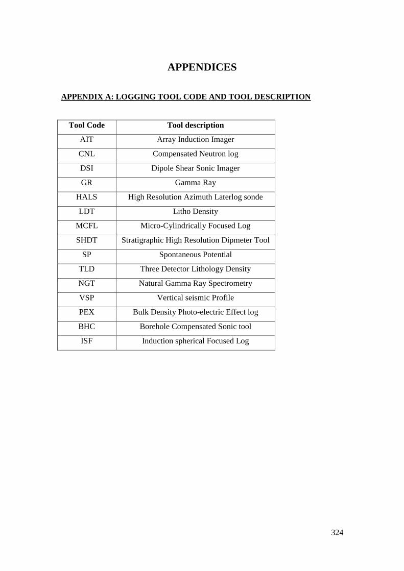
324

APPENDICES

APPENDIX A: LOGGING TOOL CODE AND TOOL DESCRIPTION

Tool Code Tool description

AIT Array Induction Imager

CNL Compensated Neutron log

DSI Dipole Shear Sonic Imager

GR Gamma Ray

HALS High Resolution Azimuth Laterlog sonde

LDT Litho Density

MCFL Micro-Cylindrically Focused Log

SHDT Stratigraphic High Resolution Dipmeter Tool

SP Spontaneous Potential

TLD Three Detector Lithology Density

NGT Natural Gamma Ray Spectrometry

VSP Vertical seismic Profile

PEX Bulk Density Photo-electric Effect log

BHC Borehole Compensated Sonic tool

ISF Induction spherical Focused Log

325

APPENDIX B: CORE PHOTOS

WELL OPI CORE PHOTOS

PHOTOS OF WELL OP3

Facies A6

Facies A5

Facies A4

Facies A3

Facies

A3

Facies

A3

Facies

A3

326

PHOTOS OF WELL OP2

WELL OP2 CORE PHOTO

Facies A4

Facies A4

Facies A5 Facies A6

Facies A6 Facies A6

Facies A1

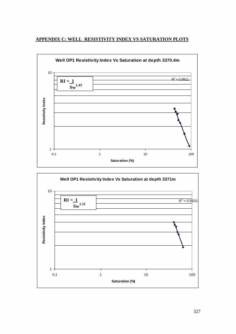
327

APPENDIX C: WELL RESISTIVITY INDEX VS SATURATION PLOTS

Well OP1 Resistivity Index Vs Saturation at depth 3370.4m

R2 = 0.9911

1

10

0.1 1 10 100

Saturation (%)

Resis

tivit

y In

dex

Well OP1 Resistivity Index Vs Saturation at depth 3371m

R2 = 0.9931

1

10

0.1 1 10 100

Saturation (%)

Re

sis

tiv

ity

In

de

x

RI = 1

Sw1.43

RI = 1

Sw1.51

328

Well OP1 Resistivity Index Vs Saturation at Depth3371.6m

R2 = 0.99

1

10

0.1 1 10 100

Saturation (%)

Re

sis

tiv

ity

In

de

x

Well OP1 Resistivity Index Vs Saturation at Depth 3372.3m

R2 = 0.977

1

10

0.1 1 10 100

Saturation (%)

Resis

tivit

y In

dex

RI = 1

Sw1.53

RI = 1

Sw1.34

329

WELL OP3 RESISTIVITY INDEX VS SATURATION PLOTS

Well OP3 Resistivity Index Vs Saturation at Depth

3283.2m

R2 = 0.9849

1

10

0.1 1 10 100

Brine saturation(%)

Resis

tivit

y In

dex

Well OP3 Resistivity Index Vs Saturation st depth 3283.4m

R2 = 0.9702

1

10

0.1 1 10 100

Brine saturation(%)

Resis

tivit

y In

dex

RI = 1

Sw1.84

RI = 1

Sw2.02

330


R2 = 0.9716

1

10

0.1 1 10 100

Saturation(%)

Resis

tivit

y In

dex

Well OP3 Resistivity Index Vs saturation at depth 3284.74m

R2 = 0.935

1

10

0.1 1 10 100

Saturation(%)

Resis

tivit

y In

dex

RI = 1

Sw1.96

RI = 1

Sw1.91

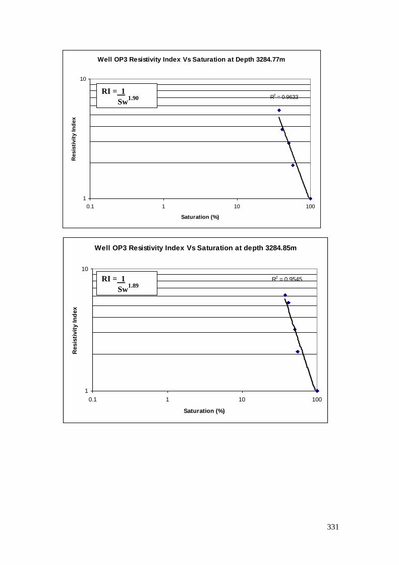
331


R2 = 0.9633

1

10

0.1 1 10 100

Saturation (%)

Resis

tivit

y In

dex

Well OP3 Resistivity Index Vs Saturation at depth 3284.85m

R2 = 0.9545

1

10

0.1 1 10 100

Saturation (%)

Resis

tivit

y In

dex

RI = 1

Sw1.90

RI = 1

Sw1.89

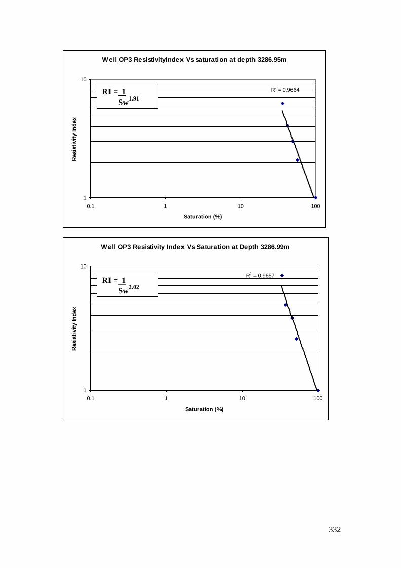
332

Well OP3 ResistivityIndex Vs saturation at depth 3286.95m

R2 = 0.9664

1

10

0.1 1 10 100

Saturation (%)

Resis

tivit

y In

dex


R2 = 0.9657

1

10

0.1 1 10 100

Saturation (%)

Resis

tivit

y In

dex

RI = 1

Sw1.91

RI = 1

Sw2.02

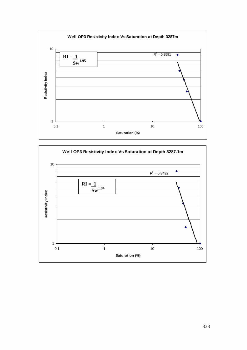
333

Well OP3 Resistivity Index Vs Saturation at Depth 3287m

R2 = 0.9591

1

10

0.1 1 10 100

Saturation (%)

Resis

tivit

y in

dex


R2 = 0.8492

1

10

0.1 1 10 100

Saturation (%)

Resis

tivit

y In

dex

RI = 1

Sw1.95

RI = 1

Sw1.94

334

APPENDIX D: WELL OP2 CAPILLARY PRESSURE DATA

Well OP2 Mercury Injection Capillary Pressure Data

Depth=3447.08m Depth=3560m Depth=3467.5m Permeability=224mD Permeability=673mD permeability=0.036mD Porosity=24.6 % Porosity=22.6% Porosity=4.6%

Injection 1.0-

Mercury Injection 1.0-

Mercury Injection 1.0-

Mercury

Pressure, Saturation, Pressure, Saturation, Pressure, Saturation,

psia fraction psia fraction psia fraction

1.01 1.000 1.01 1.000 1.08 1.000

2.01 1.000 2.01 1.000 2.07 1.000

3.00 1.000 3.00 1.000 3.07 1.000

4.01 1.000 4.01 0.984 4.06 1.000

4.99 1.000 4.99 0.939 5.06 1.000

6.0 1.000 6.0 0.824 6.1 1.000

7.5 1.000 7.5 0.700 7.5 1.000

9.0 0.988 9.0 0.636 9.0 1.000

11.0 0.910 11.0 0.593 11.0 1.000

14.0 0.757 14.0 0.558 14.0 1.000

16.9 0.695 16.9 0.554 17.0 1.000

19.9 0.662 19.9 0.547 20.0 1.000

23.0 0.640 23.0 0.535 23.0 1.000

25.9 0.627 25.9 0.527 26.0 1.000

29.9 0.614 29.8 0.516 30.2 1.000

35 0.603 35 0.508 36 1.000

40 0.592 40 0.503 40 1.000

50 0.579 50 0.494 50 1.000

60 0.568 60 0.488 61 1.000

75 0.554 75 0.478 75 0.994

90 0.541 90 0.467 90 0.989

120 0.520 120 0.451 120 0.983

150 0.505 150 0.437 150 0.977

190 0.481 190 0.420 190 0.972

250 0.452 250 0.400 250 0.966

350 0.410 350 0.374 350 0.949

450 0.380 450 0.355 450 0.938

610 0.339 610 0.335 600 0.915

800 0.295 800 0.314 820 0.893

1000 0.259 1000 0.294 1020 0.876

1300 0.222 1300 0.275 1300 0.864

1600 0.188 1600 0.246 1600 0.853

2000 0.164 2000 0.219 2000 0.842

2500 0.148 2500 0.196 2500 0.842

3100 0.136 3100 0.185 3100 0.842

4000 0.123 4000 0.174 4000 0.842

5000 0.112 5000 0.165 5000 0.842

6500 0.106 6500 0.155 6500 0.842

8000 0.099 8000 0.152 8000 0.836

10000 0.093 10000 0.144 10000 0.814

12000 0.089 12000 0.140 12000 0.780

14000 0.086 14000 0.133 14000 0.751

16900 0.079 16900 0.130 17000 0.700

20000 0.077 20000 0.121 19900 0.655

23400 0.072 23400 0.107 23400 0.599

27400 0.068 27400 0.099 27400 0.537

31400 0.061 31400 0.090 31500 0.469

35000 0.055 35000 0.081 34800 0.429

39900 0.051 39900 0.068 39800 0.361

44900 0.047 44900 0.052 45000 0.288

49800 0.041 49800 0.041 49800 0.243

54900 0.033 54900 0.030 54800 0.209

335

APPENDIX E: WELL J-FUNCTION AND HEIGHT PARAMETERS

Interfacial Tension and Contact Angle Values (Core Laboratories, 1982) used for

Well OP1 and OP3.

Wetting

Phase

Non-

Wetting

Phase

Conditions:

Température(T)

Pressure(P)

Contact

Angle(σ )

Interfacial

Tension

(dynes/cm)

Comment

Brine Oil Reservoir,T,P 30 30 Not Used

Brine Oil Laboratory,T,P 30 48 Not Used

Brine Gas Laboratory,T,P 0 72 Used

Brine Gas Reservoir,T,P 0 50 Used

Oil Gas Reservoir,T,P 0 4 Not Used

Gas Mercury Laboratory,T,P 140 480 Not used

WELL OP1 J-FUNCTION PARAMETERS

Depth=3370.4m;K=38mD;Poro=0.177

Brine SW Pc Pc*coso cos lab Pc res 0.3048*Pc Ht Nor(J(Sw)

90.5 2 100 72 1.388889 0.423333 1.286727 0.09

71 4 200 72 2.777778 0.846667 2.573455 0.18

57.1 8 400 72 5.555556 1.693333 5.14691 0.35

52.4 15 750 72 10.41667 3.175 9.650456 0.66

49.8 35 1750 72 24.30556 7.408333 22.51773 1.54

46.2 80 4000 72 55.55556 16.93333 51.4691 3.53

43.2 180 9000 72 125 38.1 115.8055 7.93

Depth=3371.0m;K=38mD;Poro=.186

Brine Sw Pc

64 4 200 72 2.777778 0.846667 2.573455 0.17

51.1 8 400 72 5.555556 1.693333 5.14691 0.34

47.5 15 750 72 10.41667 3.175 9.650456 0.64

45.2 35 1750 72 24.30556 7.408333 22.51773 1.5

42.3 80 4000 72 55.55556 16.93333 51.4691 3.44

39.7 180 9000 72 125 38.1 115.8055 7.74

Depth=3371.6m;K=17mD;Poro=0.167

Brine Sw Pc

74.9 4 200 72 2.777778 0.846667 2.573455 0.12

55.9 8 400 72 5.555556 1.693333 5.14691 0.24

50.8 15 750 72 10.41667 3.175 9.650456 0.46

48.2 35 1750 72 24.30556 7.408333 22.51773 1.06

44.5 80 4000 72 55.55556 16.93333 51.4691 2.43

42.4 180 9000 72 125 38.1 115.8055 5.47

Depth=3372.3m;K=1.1mD;Poro=0.117

Brine Sw Pc

71.3 15 750 72 10.41667 3.175 9.650456 0.14

63.7 35 1750 72 24.30556 7.408333 22.51773 0.33

56.7 80 4000 72 55.55556 16.93333 51.4691 0.75

52.2 180 9000 72 125 38.1 115.8055 1.68

336

WELL OP3 J-FUNCTION AND HEIGHT PARAMETERS

WELL OP3 J-FUNCTION PARAMETERS

Depth(m) Sw(%) Pc(psi) Pc Cosθ Cosθ lab Pc res 0.3048*Pc Ht Nor(J Sw)

3283.2 100 1 50 72 0.694444 0.211667 0.643364 0.02

100 2 100 72 1.388889 0.423333 1.286727 0.03

K=6mD 98.4 4 200 72 2.777778 0.846667 2.573455 0.07

82.7 8 400 72 5.555556 1.693333 5.14691 0.13

Porosity=20.2 71.4 15 750 72 10.41667 3.175 9.650456 0.25

63.2 35 1750 72 24.30556 7.408333 22.51773 0.57

53.3 100 5000 72 69.44444 21.16667 64.33637 1.64

50 180 9000 72 125 38.1 115.8055 2.95

3283.4 100 1 50 72 0.694444 0.211667 0.643364 0.01

100 2 100 72 1.388889 0.423333 1.286727 0.03

K=4.4mD 97.9 4 200 72 2.777778 0.846667 2.573455 0.06

83.9 8 400 72 5.555556 1.693333 5.14691 0.12

Porosity=18.7 71.2 15 750 72 10.41667 3.175 9.650456 0.22

62.7 35 1750 72 24.30556 7.408333 22.51773 0.51

55.7 100 5000 72 69.44444 21.16667 64.33637 1.46

52.1 180 9000 72 125 38.1 115.8055 2.63

3283.5 100 1 50 72 0.694444 0.211667 0.643364 0.01

100 2 100 72 1.388889 0.423333 1.286727 0.03

K=3.5 97.8 4 200 72 2.777778 0.846667 2.573455 0.05

87.6 8 400 72 5.555556 1.693333 5.14691 0.11

Porosity=17.7 72.8 15 750 72 10.41667 3.175 9.650456 0.2

63.5 35 1750 72 24.30556 7.408333 22.51773 0.47

55.9 100 5000 72 69.44444 21.16667 64.33637 1.34

51.6 180 9000 72 125 38.1 115.8055 2.41

3284.74 100 1 50 72 0.694444 0.211667 0.643364 0.06

94.8 2 100 72 1.388889 0.423333 1.286727 0.11

K=80mD 67.6 4 200 72 2.777778 0.846667 2.573455 0.22

59.8 8 400 72 5.555556 1.693333 5.14691 0.44

Porosity=23.5 54.9 15 750 72 10.41667 3.175 9.650456 0.83

48.1 35 1750 72 24.30556 7.408333 22.51773 1.94

40.3 100 5000 72 69.44444 21.16667 64.33637 5.55

37.9 180 9000 72 125 38.1 115.8055 9.99

3284.77 100 1 50 72 0.694444 0.211667 0.643364 0.05

95.7 2 100 72 1.388889 0.423333 1.286727 0.09

K=57mD 72.6 4 200 72 2.777778 0.846667 2.573455 0.19

62.9 8 400 72 5.555556 1.693333 5.14691 0.38

Porosity=23.4 57.6 15 750 72 10.41667 3.175 9.650456 0.7

50.5 35 1750 72 24.30556 7.408333 22.51773 1.64

41.2 100 5000 72 69.44444 21.16667 64.33637 4.69

38 180 9000 72 125 38.1 115.8055 8.45

3284.85 100 1 50 72 0.694444 0.211667 0.643364 0.05

96.1 2 100 72 1.388889 0.423333 1.286727 0.1

K=69mD 68.4 4 200 72 2.777778 0.846667 2.573455 0.21

60.4 8 400 72 5.555556 1.693333 5.14691 0.41

Porosity=23.6 55.2 15 750 72 10.41667 3.175 9.650456 0.77

49.7 35 1750 72 24.30556 7.408333 22.51773 1.8

40.9 100 5000 72 69.44444 21.16667 64.33637 5.14

37.4 180 9000 72 125 38.1 115.8055 9.26

3286.95 97.9 1 50 72 0.694444 0.211667 0.643364 0.05

85.8 2 100 72 1.388889 0.423333 1.286727 0.09

K=59mD 68 4 200 72 2.777778 0.846667 2.573455 0.19

61.2 8 400 72 5.555556 1.693333 5.14691 0.38

Porosity=24.2 56 15 750 72 10.41667 3.175 9.650456 0.7

49 35 1750 72 24.30556 7.408333 22.51773 1.64

41.8 100 5000 72 69.44444 21.16667 64.33637 4.69

36.3 180 9000 72 125 38.1 115.8055 8.45

3286.99 98.2 1 50 72 0.694444 0.211667 0.643364 0.06

80.7 2 100 72 1.388889 0.423333 1.286727 0.13

K=105mD 62.9 4 200 72 2.777778 0.846667 2.573455 0.25

57.2 8 400 72 5.555556 1.693333 5.14691 0.5

Porosity=24.3 52.4 15 750 72 10.41667 3.175 9.650456 0.94

45.5 35 1750 72 24.30556 7.408333 22.51773 2.19

37.3 100 5000 72 69.44444 21.16667 64.33637 6.26

33 180 9000 72 125 38.1 115.8055 11.26

3287 97.6 1 50 72 0.694444 0.211667 0.643364 0.05

78.7 2 100 72 1.388889 0.423333 1.286727 0.11

K=79mD 60.9 4 200 72 2.777778 0.846667 2.573455 0.22

55.4 8 400 72 5.555556 1.693333 5.14691 0.43

Porosity=24.3 50.7 15 750 72 10.41667 3.175 9.650456 0.81

44.4 35 1750 72 24.30556 7.408333 22.51773 1.89

35.9 100 5000 72 69.44444 21.16667 64.33637 5.42

32.5 180 9000 72 125 38.1 115.8055 9.75

3287.1 97.1 1 50 72 0.694444 0.211667 0.643364 0.06

78.8 2 100 72 1.388889 0.423333 1.286727 0.12

K=90mD 60.7 4 200 72 2.777778 0.846667 2.573455 0.23

55 8 400 72 5.555556 1.693333 5.14691 0.46

Porosity=24.4 50.4 15 750 72 10.41667 3.175 9.650456 0.87

44.2 35 1750 72 24.30556 7.408333 22.51773 2.02

35.7 100 5000 72 69.44444 21.16667 64.33637 5.78

32.4 180 9000 72 125 38.1 115.8055 10.39

337

APPENDIX F: NEUTRON VERSUS DENSITY AND GR LOG PLOTS

Well MA1

Neutron versus Density and GR Plot

-0.05 0.05 0.15 0.25 0.35 0.45

Neutron (v/v)

3.

2.8

2.6

2.4

2.2

2.

De

ns

ity

(g

/cc

)

Clean Sand

Shaly Sands

Shaly

Shale

0.

150.

GR

SS 0

10

20

30

40

LS 0

10

20

30

40

DOL 0

10

20

30

40

(SWS) Density Neutron(NPHI) Overlay, Rhofluid = 1.0 (CP-1c 1989)

Well MA3


-0.05 0.05 0.15 0.25 0.35 0.45

Neutron (v/v)

3.

2.8

2.6

2.4

2.2

2.

De

ns

ity

(g

/cc

)

Clean Sand

Shaly Sands

Shaly

Shale

0.

150.

GR

SS 0

10

20

30

40

LS 0

10

20

30

40

DOL 0

10

20

30

40


Well MA2

Neutron Versus Density and GR Plot

-0.05 0.05 0.15 0.25 0.35 0.45

Neutron (v/v)

3.

2.8

2.6

2.4

2.2

2.

De

ns

ity

(g

/cc

)

Clean Sand

Shaly Sands

Shaly

Shale

0.

150.

GR

SS 0

10

20

30

40

LS 0

10

20

30

40

DOL 0

10

20

30

40


Well OP4


-0.05 0.05 0.15 0.25 0.35 0.45

Neutron (v/v)

3.

2.8

2.6

2.4

2.2

2.

De

ns

ity

(g

/cc

)

Clean Sand

Shaly Sands

Shaly

Shale

0.

150.

GR

SS 0

10

20

30

40

LS 0

10

20

30

40

DOL 0

10

20

30

40


Wet

clay

point

Well OP1

Neutron Versus Density and GR PLot

-0.05 0.05 0.15 0.25 0.35 0.45

Neutron (v/v)

3.

2.8

2.6

2.4

2.2

2.

De

ns

ity

(g

/cc

)

Clean Sand

Shaly Sands

Shaly

Shale

0.

150.

GR

SS 0

10

20

30

40

LS 0

10

20

30

40

DOL 0

10

20

30

40


Well OP5

Neutron Versus Density and GR Plot

-0.05 0.05 0.15 0.25 0.35 0.45

Neutron (v/v)

3.

2.8

2.6

2.4

2.2

2.

De

ns

ity

(g

/cc

)

Clean Sand

Shaly Sands

Shaly

Shale

0.

150.

GR

SS 0

10

20

30

40

LS 0

10

20

30

40

DOL 0

10

20

30

40


Wet

Clay

point

Wet Clay

Point

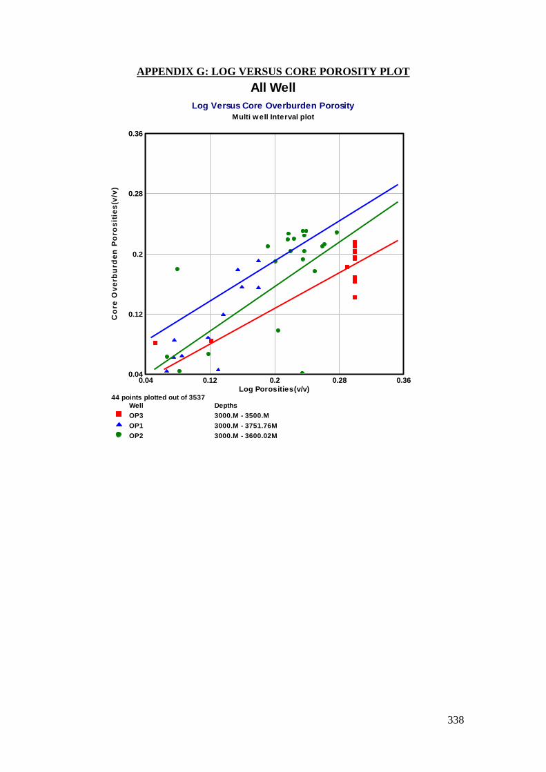
338

APPENDIX G: LOG VERSUS CORE POROSITY PLOT All Well

Log Versus Core Overburden Porosity

Multi well Interval plot

0.04 0.12 0.2 0.28 0.36

Log Porosities(v/v)

0.04

0.12

0.2

0.28

0.36

Co

re O

ve

rbu

rde

n P

oro

sit

ies

(v/v

)

44 points plotted out of 3537

Well Depths

OP3 3000.M - 3500.M

OP1 3000.M - 3751.76M

OP2 3000.M - 3600.02M

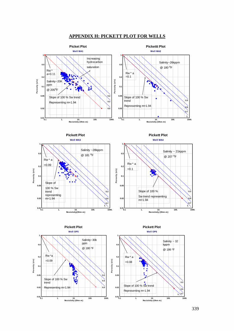
339

APPENDIX H: PICKETT PLOT FOR WELLS

Picket Plot

Well MA1

0.1 1. 10. 100. 1000.

Resistivity (Ohm-m)

0.01

0.02

0.05

0.1

0.2

0.5

1.

Po

ros

ity

(v

/v)

0.2

0.3

0.5


Representing m=1.94

Rw *

a=0.11

Increasing

hydrocarbon

saturation

Pickettt Plot

Well MA2

0.1 1. 10. 100. 1000.

Resistivity (Ohm-m)

0.01

0.02

0.05

0.1

0.2

0.5

1.

Po

ros

ity

(v

/v)

0.3

0.5

0.7

1.

Slope of 100 % Sw

trend

Representing m=1.94

Rw * a

=0.1

Salinity~20K

ppm

@ 205oF

Salinity~26kppm

@ 180 oF

Pickett Plot

Well MA3

0.1 1. 10. 100. 1000.

Resistivity(Ohm-m)

0.01

0.02

0.05

0.1

0.2

0.5

1.

Po

ros

ity

(v

/v)

0.3

0.5

0.7

1.

Pickett Plot

Well MA4

0.1 1. 10. 100. 1000.

Resistivity (Ohm-m)

0.01

0.02

0.05

0.1

0.2

0.5

1.

Po

ros

ity

(v

/v)

0.3

0.5

0.7

1.

Slope of

100 % Sw

trend

representing

m=1.94

Rw * a

=0.09

Slope of 100 %

Sw trend representing

m=1.94

Rw * a

=0.1

Salinity ~28kppm

@ 181 oF

Salinity ~ 21kppm

@ 207 oF

Pickett Plot

Well OP5

0.1 1. 10. 100. 1000.

Resistivity (Ohm-m)

0.01

0.02

0.05

0.1

0.2

0.5

1.

Po

ros

ity

(v

/v)

0.2

0.3

0.5

Pickett Plot

Well OP6

0.1 1. 10. 100. 1000.

Resistivity (Ohm-m)

0.01

0.02

0.05

0.1

0.2

0.5

1.

Po

ros

ity

(v

/v)

0.3

0.5

0.71.

Slope of 100 % Sw

trend

Representing m=1.94

Rw *a

=0.09


Representing m=1.94

Rw * a

=0.08

Salinity~30k

ppm

@ 180 oF

Salinity ~ 32

kppm

@ 186 oF

340

APPENDIX I: RESULTS OF RFT MEASUREMENTS FOR WELLS

WELL OP2

DEPTH IHP FHP

PRE-TEST DATA

(primary gauge) (primary gauge) Vol Time Flow SIP SIP SIP Temp Mobility

meters feet Set time EMW to

RT EMW to

SS

(RTMD) (TVDmd) (psia) (psia) (cc) (mins) (psia) (ppg) (ppg) (deg F) (md/cp)

3448.0 11312.3 6113.3 6102.1 20.0 3:15 10.0 5085.24 8.644817 8.7084812 197.3 91.9

3449.0 11315.6 6099.8 6097.4 20.0 3:36 3.0 5086.46 8.6443839 8.7080263 205.0 165.0

3450.0 11318.9 6067.0 6067.0 20.0 4:44 4.0 5083.90 8.6375288 8.7011022 209.3 507.0

3451.5 11323.8 6102.4 6099.5 20.0 3:32 3.5 5090.93 8.6457138 8.7093196 201.8 70.4

3453.0 11328.7 6099.0 6090.0 20.0 3:43 15.0 5179.38 8.7921037 8.8567582 203.3 3.4

3454.5 11333.7 6078.4 6078.7 20.0 4:32 5.0 5092.01 8.6400381 8.7035465 208.8 58.9

3456.0 11338.6 6095.8 6093.4 20.0 4:02 6.0 5095.20 8.6416984 8.7051913 206.2 223.6

3456.5 11340.2 6089.5 6083.7 20.0 4:12 15.0 5392.13 9.1439827 9.2111563 207.4 12.7

C

o

r

e

341

Well OP3

P mud

Depth

P mud

Before

P res

psia

After

psia From To QC Remarks

3276.04 5735 4854 5735 13:31 13:38 1

Drawdown to 550psi, Erratic BU

Plugging (?) building slowly at end

3278.05 5741 4865 5740 13:39 13:49 1

Deep drawdown to 250psi slow but

smooth BU. Still Building

3280.05 5745 4838 5744 13:50 13:56 2

Deep drawdown to 500psi Reasonable

BU. Stabilizing at end

3282.04 5749 4842 5749 13:58 14:05 2

Deep drawdown to 500psi, rapid BU,

Fairly stable

3283.05 5751 4838 5751 14:06 14:11 4 shallow drawdown, stable

3284.05 5754 4838 5754 14:12 14:16 4 Very shallow drawdown, stable at end.

3285.04 5756 4840 5756 14:18 14:23 4 Very shallow drawdown, stable at end.

3312.05 5804 4885 5803 14:27 14:33 4 shallow drawdown, stable at end.

3314.05 5808 5806 14:33 14:39 0 Drawdown to 160psi, no BU

3316.04 5812 4891 5811 1441 14:46 4 Very shallow drawdown, stable

3322.05 5826 leakage 5825 14:48 14:57 0

Deep drawdown to 170psi, BU to 5323,

then down to 5034 (not stable)

3355.04 5883 4972 5881 15:01 15:06 4 Very shallow drawdown, stable





3365.04 5902 4982 5902 15:32 15:37 4 Low drawdown, stable

3367.05 5907 4986 5907 15:39 15:43 4 Very low drawdown, stable

3369.55 5913 4990 5912 15:46 15:50 3 medium drawdown, stable

Time

342

WELL OP4

DEPTH IHP FHP PRE-TEST DATA

(primary gauge) (primary gauge) Vol Time Flow SIP SIP SIP Temp Mobility

meters feet Set time EMW to RT EMW to SS

(RTMD) (TVDmd) (psia) (psia) (cc) (mins) (psia) (ppg) (ppg) (deg F) (md/cp)

3240.0 10629.9 5679.0 5675.6 20.0 16:04 4.6 4929.75 8.9184933 8.9884226 227.0 91.5

3240.0 10629.9 5674.4 5668.8 20.0 13:32 8.0 4924.64 8.9092487 8.9791055 221.0

3241.0 10633.2 5684.8 5684.4 20.0 20:13 5.0 4933.60 8.9227045 8.992645 229.0 245.2

3242.0 10636.5 5686.3 5686.1 20.0 20:04 4.2 4933.39 8.9195726 8.9894668 229.0 92.1

3243.0 10639.8 5688.6 5687.9 20.0 19:55 4.0 4933.82 8.9175994 8.9874564 229.0 68.6

3244.0 10643.0 5680.4 5675.6 20.0 13:46 9.0 4925.71 8.9001966 8.9698956 224.0 76.0

3246.0 10649.6 5688.3 5685.5 20.0 15:08 2.5 4931.52 8.9052043 8.9748993 227.0 561.9

3247.0 10652.9 5694.6 5694.3 20.0 19:44 5.0 4935.82 8.9102242 8.9799368 229.0 1.1

3248.0 10656.2 5690.2 5686.8 20.0 15:15 4.0 4931.25 8.8992336 8.9688386 226.0 246.5

3249.0 10659.4 5703.0 5698.2 20.0 19:20 18.0 4936.70 8.9063269 8.9759658 229.0 331.9

3250.0 10662.7 5693.3 5891.2 20.0 15:26 8.5 4932.55 8.8961017 8.9656391 226.0 186.7

3253.0 10672.6 5700.2 5704.4 20.0 15:41 4.0 0 0 226.0

3255.0 10679.1 5702.4 5700.3 20.0 15:50 0 0 227.0

3255.2 10679.8 5702.6 5707.1 20.0 15:57 0 0 227.0

3257.0 10685.7 5713.7 5701.1 20.0 14:01 19.0 4930.17 8.8726988 8.9419031 225.0 86.3

3287.5 10785.8 5782.9 5769.7 20.0 18:33 29.5 5247.40 9.3559957 9.4282873 233.0 0.1

3288.5 10789.0 5780.4 5760.2 20.0 14:30 28.0 5036.42 8.9770925 9.0464351 227.0 0.5

3301.0 10830.1 5821.3 5791.5 20.0 16:20 24.1 5007.70 8.8921009 8.9605249 230.0 20.4

343

WELL OP6

DEPTH IHP FHP PRE-TEST DATA

(primary gauge) (primary gauge) Vol Time Flow SIP SIP SIP Temp

meters feet Set time EMW to RT EMW to SS

(RTMD) (TVDmd) (psia) (psia) (cc) (mins) (psia) (ppg) (ppg) (deg F)

3199.5 10414.4 5799.6 5787.6 20.0 23:36 5.0 4642.88 8.573361 8.6419866 206.0

3200.5 10417.7 5783.5 5776.1 20.0 23:50 10.0 4645.47 8.5754428 8.6440633 208.0

3201.5 10420.9 5775.6 5776.3 20.0 0:06 10.0 4646.27 8.5742192 8.6428081 209.0

3206.0 10435.7 5789.6 5783.1 20.0 0:23 11.0 4646.69 8.5628627 8.631263 210.0

3216.0 10468.5 5808.9 5798.9 20.0 1:30 11.0 4665.00 8.5696626 8.637901 212.0

3217.0 10471.8 5800.0 5800.6 20.0 1:47 4.0 4665.85 8.5685385 8.6367465 212.0

3218.0 10475.1 5800.7 5802.0 20.0 1:56 7.0 4666.85 8.5676905 8.6358702 212.0

3219.5 10480.0 5802.3 5803.8 20.0 2:08 9.5 4666.95 8.563851 8.6319678 212.0

3221.0 10484.9 5805.5 5806.1 20.0 2:23 10.0 4670.93 8.5671307 8.6352414 213.0

3222.5 10489.8 5809.7 5797.2 20.0 2:38 6.0 4668.12 8.5579601 8.6259658 214.0

3225.0 10498.0 5815.4 5814.9 20.0 2:48 6.0 4671.42 8.557319 8.625266 214.0

3226.0 10501.3 5812.1 5817.3 20.0 3:00 7.5 4673.90 8.5591869 8.6271273 215.0

3227.0 10504.6 5814.1 5814.6 20.0 3:12 10.0 4671.10 8.5513876 8.6192447 215.0

3228.0 10507.9 5813.9 5817.6 20.0 3:27 10.0 4677.73 8.5608512 8.6287621 216.0

WELL MA1

STRAIN GAUGE

DEPTH

HYD

PRESSU

RE

EMW

FORMATIO

N

PRESSURE

EMWHYD

PRESSUREEMW

HYD

PRESSUREEMW

FORMATI

ON

PRESSU

RE

EMWHYD

PRESSUREEMW

(m MD) (mTVD)(mTVDS

S) (MSL)BEFORE

ppg

EMW

ppg

EMWAFTER

ppg

EMWBEFORE

ppg

EMW

ppg

EMWAFTER

ppg

EMW

3213.4 3213.4 3191.9 5557.06 10.14 4733.27 8.69 5557.01 10.14 5572.6 10.16 4749.3 8.72 5572.8 10.17

3217.7 3217.7 3196.2 5564.20 10.14 4736.99 8.69 5564.56 10.14 5580.3 10.17 4751.6 8.71 5580.4 10.17

3219.0 3219.0 3197.5 5566.71 10.14 4738.56 8.69 5566.72 10.14 5582.6 10.17 4753.1 8.71 5582.5 10.17

3220.0 3220.0 3198.5 5568.21 10.14 4739.80 8.69 5568.44 10.14 5584.2 10.17 4754.4 8.71 5684.2 10.35

3222.5 3222.5 3201.0 5572.53 10.14 4743.22 8.69 5572.61 10.14 5588.6 10.17 4757.9 8.71 5588.4 10.17

3223.2 3223.2 3201.7 5573.65 10.14 4744.09 8.69 5573.54 10.14 5589.4 10.16 4758.8 8.71 5588.3 10.16

3227.0 3227.0 3205.5 5580.11 10.14 4749.77 8.69 5580.11 10.14 5595.9 10.16 4764.3 8.71 5595.7 10.16

3228.5 3228.5 3207.0 5582.51 10.14 4751.81 8.69 5582.41 10.14 5598.4 10.16 4766.5 8.71 5598.1 10.16

3231.3 3231.3 3209.8 5587.18 10.14 4755.93 8.69 5587.14 10.14 5603.0 10.16 4770.5 8.71 5602.8 10.16

3233.0 3233.0 3211.5 5589.78 10.13 4761.40 8.69 5589.27 10.13 5605.7 10.16 4777.4 8.72 5606.4 10.16

3236.2 3236.2 3214.7 5594.77 10.13 4762.64 8.68 5594.86 10.13 5611.0 10.16 4777.3 8.71 5610.6 10.16

HP GAUGE

344

WELL MA2:

HP GAUGE

DEPTH HYD

PRESSURE EMW

FORMATION PRESSURE

EMW HYD

PRESSURE EMW

(m MD) (mTVD) (mTVDSS)

(MSL) BEFORE ppg ppg AFTER ppg

2944.5 2941.5 2920.0 5143.8 10.25 4359.5 8.75 5143.7 10.25

2945.5 2942.5 2921.0 5145.6 10.25 4361.2 8.75 5145.3 10.25

2947.0 2944.0 2922.5 5148.3 10.25 4363.3 8.75 5147.9 10.25

2952.0 2949.0 2927.5 5156.6 10.25 4371.6 8.75 5156.3 10.25

2960.5 2957.5 2936.0 5170.3 10.25 4387.1 8.76 5169.9 10.25

2963.5 2960.5 2939.0 5175.5 10.25 4389.2 8.75 5175.1 10.25

2965.3 2962.3 2940.8 5178.8 10.25 4389.0 8.75 5178.2 10.25

2967.2 2964.2 2942.7 5181.3 10.25 4391.2 8.75 5180.8 10.24

2967.8 2964.8 2943.3 5182.0 10.25 4391.9 8.75 5181.7 10.24

2968.5 2965.5 2944.0 5183.2 10.25 4393.1 8.75 5182.9 10.24

2974.0 2971.0 2949.5 5192.2 10.24 4401.4 8.75 5191.6 10.24

2974.8 2971.8 2950.3 5191.9 10.24 4401.2 8.74 5191.6 10.24

2977.7 2974.7 2953.2 5197.8 10.24 4407.5 8.75 5197.1 10.24

2979.0 2976.0 2954.5 5199.5 10.24 4408.3 8.75 5198.9 10.24

2982.0 2979.0 2957.5 5203.7 10.24 4412.1 8.74 5203.2 10.24

2960.0 2957.0 2935.5 5165.2 10.24 4387.8 8.76 5165.1 10.24

2963.0 2960.0 2938.5 5170.3 10.24 4389.2 8.76 5169.9 10.24

2964.0 2961.0 2939.5 5172.0 10.24 4389.3 8.75 5171.7 10.24

2965.8 2962.8 2941.3 5175.2 10.24 4389.8 8.75 5174.7 10.24

345

WELL MA3

HP GAUGE

DEPTH HYD

PRESSURE EMW

FORMATION PRESSURE

EMW HYD

PRESSURE EMW

(m MD) (mTVD) (mTVDSS)

(MSL) BEFORE ppg ppg AFTER ppg

2944.5 2941.5 2920.0 5143.8 10.25 4359.5 8.75 5143.7 10.25

2945.5 2942.5 2921.0 5145.6 10.25 4361.2 8.75 5145.3 10.25

2947.0 2944.0 2922.5 5148.3 10.25 4363.3 8.75 5147.9 10.25

2952.0 2949.0 2927.5 5156.6 10.25 4371.6 8.75 5156.3 10.25

2960.5 2957.5 2936.0 5170.3 10.25 4387.1 8.76 5169.9 10.25

2963.5 2960.5 2939.0 5175.5 10.25 4389.2 8.75 5175.1 10.25

2965.3 2962.3 2940.8 5178.8 10.25 4389.0 8.75 5178.2 10.25

2967.2 2964.2 2942.7 5181.3 10.25 4391.2 8.75 5180.8 10.24

2967.8 2964.8 2943.3 5182.0 10.25 4391.9 8.75 5181.7 10.24

2968.5 2965.5 2944.0 5183.2 10.25 4393.1 8.75 5182.9 10.24

2974.0 2971.0 2949.5 5192.2 10.24 4401.4 8.75 5191.6 10.24

2974.8 2971.8 2950.3 5191.9 10.24 4401.2 8.74 5191.6 10.24

2977.7 2974.7 2953.2 5197.8 10.24 4407.5 8.75 5197.1 10.24

2979.0 2976.0 2954.5 5199.5 10.24 4408.3 8.75 5198.9 10.24

2982.0 2979.0 2957.5 5203.7 10.24 4412.1 8.74 5203.2 10.24

2960.0 2957.0 2935.5 5165.2 10.24 4387.8 8.76 5165.1 10.24

2963.0 2960.0 2938.5 5170.3 10.24 4389.2 8.76 5169.9 10.24

2964.0 2961.0 2939.5 5172.0 10.24 4389.3 8.75 5171.7 10.24

2965.8 2962.8 2941.3 5175.2 10.24 4389.8 8.75 5174.7 10.24

PETROPHYSICAL EVALUATION OF THE ALBIAN AGE GAS … · Petrophysical evaluation of the Albian age...

Documents

Transcript of PETROPHYSICAL EVALUATION OF THE ALBIAN AGE GAS … · Petrophysical evaluation of the Albian age...