Petri Nets Lecture Notes for SS 2015 - TUM - Chair VII · Petri Nets Lecture Notes for SS 2015...
80
Petri Nets Lecture Notes for SS 2015 Prof. Javier Esparza July 16, 2015
Transcript of Petri Nets Lecture Notes for SS 2015 - TUM - Chair VII · Petri Nets Lecture Notes for SS 2015...
Petri Nets
Lecture Notes for SS 2015
Prof. Javier Esparza
July 16, 2015

2

Contents
I Petri Nets: Syntax, Semantics, Models 7
1 Basic definitions 9
1.1 Preliminaries . . . . . . . . . . . . . . . . . . . . . . . . . . . . . . 9
1.2 Syntax . . . . . . . . . . . . . . . . . . . . . . . . . . . . . . . . . . 10
1.3 Semantics . . . . . . . . . . . . . . . . . . . . . . . . . . . . . . . . 12
2 Modelling with Petri nets 17
2.1 A buffer of capacity n . . . . . . . . . . . . . . . . . . . . . . . . . . 17
2.2 Train tracks . . . . . . . . . . . . . . . . . . . . . . . . . . . . . . . 18
2.3 Dining philosophers . . . . . . . . . . . . . . . . . . . . . . . . . . . 20
2.4 A logical puzzle . . . . . . . . . . . . . . . . . . . . . . . . . . . . . 20
2.5 Peterson’s algorithm . . . . . . . . . . . . . . . . . . . . . . . . . . 22
2.6 The action/reaction protocol . . . . . . . . . . . . . . . . . . . . . . 22
2.7 Variants of the main model . . . . . . . . . . . . . . . . . . . . . . . 24
2.8 Analysis problems . . . . . . . . . . . . . . . . . . . . . . . . . . . 28
II Analysis Techniques for Petri Nets 31
3 Decision procedures 35
3.1 A decision procedure for Boundedness . . . . . . . . . . . . . . . . 35
3.2 Decision procedures for Coverability . . . . . . . . . . . . . . . . . 37
3.2.1 Coverability graphs . . . . . . . . . . . . . . . . . . . . . . . 37
3.2.2 Rackoff’s theorem . . . . . . . . . . . . . . . . . . . . . . . 40
3.2.3 The backwards-reachability algorithm . . . . . . . . . . . . . 43
3.3 Decision procedures for other problems . . . . . . . . . . . . . . . . 46
3.3.1 Reachability . . . . . . . . . . . . . . . . . . . . . . . . . . 46
3.3.2 Deadlock-freedom . . . . . . . . . . . . . . . . . . . . . . . 47
3.3.3 Liveness . . . . . . . . . . . . . . . . . . . . . . . . . . . . 50
3.4 Complexity . . . . . . . . . . . . . . . . . . . . . . . . . . . . . . . 50
3.5 Algorithms for bounded Petri nets . . . . . . . . . . . . . . . . . . . 51
3

4 CONTENTS
4 Semi-decision procedures 53
4.1 Linear systems of equations and linear programming . . . . . . . . . 53
4.2 The Marking Equation . . . . . . . . . . . . . . . . . . . . . . . . . 54
4.3 S- and T-invariants . . . . . . . . . . . . . . . . . . . . . . . . . . . 57
4.3.1 S-invariants . . . . . . . . . . . . . . . . . . . . . . . . . . . 57
4.3.2 T-invariants . . . . . . . . . . . . . . . . . . . . . . . . . . . 60
4.4 Siphons and Traps . . . . . . . . . . . . . . . . . . . . . . . . . . . . 61
4.4.1 Siphons . . . . . . . . . . . . . . . . . . . . . . . . . . . . . 61
4.4.2 Traps . . . . . . . . . . . . . . . . . . . . . . . . . . . . . . 63
5 Petri net classes with efficient decision procedures 67
5.1 S-Systems . . . . . . . . . . . . . . . . . . . . . . . . . . . . . . . . 68
5.2 T-systems . . . . . . . . . . . . . . . . . . . . . . . . . . . . . . . . 69
5.2.1 Liveness . . . . . . . . . . . . . . . . . . . . . . . . . . . . 69
5.2.2 Boundedness . . . . . . . . . . . . . . . . . . . . . . . . . . 70
5.2.3 Reachability . . . . . . . . . . . . . . . . . . . . . . . . . . 71
5.2.4 Other properties . . . . . . . . . . . . . . . . . . . . . . . . 72
5.3 Free-Choice Systems . . . . . . . . . . . . . . . . . . . . . . . . . . 74
5.3.1 Liveness . . . . . . . . . . . . . . . . . . . . . . . . . . . . 74
5.3.2 Boundedness . . . . . . . . . . . . . . . . . . . . . . . . . . 76
5.3.3 Reachability . . . . . . . . . . . . . . . . . . . . . . . . . . 80

CONTENTS 5
Sources
The main sources are:
J. Desel. Struktur und Analyse von Free-Choice-Petrinetzen. Deutscher
Universitats Verlag, 1992.
J. Desel und J. Esparza. Free-choice Petri nets. Cambridge Tracts in
Theoretical Computer Science 40, Cambridge University Press, 1995.
The Petri net model of Peterson’s algorithm is taken from
E. Best. Semantics of Sequential and Parallel Programs. Prentice-Hall,
1996.
The action-reaction protocol is taken from
R. Walter. Petrinetzmodelle verteilter Algorithmen – Intuition und Be-
weistechnik. Dieter Bertz Verlag, 1996.
The train examples of Chapter 2 belong to the Petri net folklore. They were first
introduced by H. Genrich.

6 CONTENTS
Part I
Petri Nets: Syntax, Semantics,
Models
7


Chapter 1
Basic definitions
1.1 Preliminaries
Numbers
N, Z, Q and R denote the natural, rational, and real numbers.
Relations
Let X be a set and R ⊆ X × X a relation. R∗ denotes the transitive and reflexive
closure of R. R−1 is the inverse of R, that is, the relation defined by (x, y) ∈ R−1 ⇔(y, x) ∈ R.
Sequences
A finite sequence over a set A is a mapping σ : {1, . . . , n} → A, denoted by the string
a1a2 . . . an, where ai = σ(i) for every 1 ≤ i ≤ n, or the mapping ǫ : ∅ → A, the
empty sequence. The length of σ is n and the length of ǫ is 0.
An infinite sequence is a mapping σ : IN → A. We write σ = a1a2a3 . . . with
ai = σ(i).The concatenation of two finite sequences or of a finite and an infinite sequence is
defined as usual. Given a finite sequence σ, we denote by σω the infinite concatenation
σσσ . . ..
σ is a prefix of τ if σ = τ or σσ′ = τ for some sequence σ′.
The alphabet of a sequence σ is the set of elements of A occurring in σ. Given
a sequence σ over A and B ⊆ A, the projection or restriction σ|B is the result of
removing all occurrences of elements a ∈ A \B in σ.
Vectors and matrices
Let A = {a1, . . . , an} be a finite set and let K be one of N,Z,Q,R.
9

10 CHAPTER 1. BASIC DEFINITIONS
We represent a mapping X : A → K by the vector (X(a1), . . . , X(an)). We
identify the mapping X and its vector representation.
Given vectors X = (x1, . . . , xn) and Y = (y1, . . . , yn), the (scalar) product X ·Yis the number x1y1 + . . . + xnyn (we do not distinguish between row and column
vectors!). We write X ≥ Y to denote x1 ≥ y1 ∧ . . . ∧ xn ≥ yn,a nd X > Y to denote
x1 > y1 ∧ . . . ∧ xn > yn.
Let B = {b1, . . . , bm} be a finite set. A mapping C : A × B → K is represented
by the n×m matrix
C(a1, b1) C(a1, b2) · · · C(a1, bm)C(a2, b1) C(a2, b2) · · · C(a2, bm)· · · · · · · · · · · ·
C(an, b1) C(an, b2) · · · C(an, bm)
We also write C = (cij)i=1,...,n,j=1,...,m, where cij = C(ai, bj).Let X = (x1, . . . , xm) be a vector and let C be a n×m matrix. The product C ·X
is the vector Y = (y1, . . . , yn) given by
y(i) = ci1x1 + . . .+ cimxm
and for X = (x1, . . . , xn) the product X · C is the vector Y = (y1, . . . , ym) given by
y(i) = c1ix1 + . . .+ cnixn
1.2 Syntax
Definition 1.2.1 (Net, preset, postset)
A net N = (S, T, F ) consists of a finite set S of places (represented by circles), a
finite set T of transitions disjoint from S (squares), and a flow relation (arrows) F ⊆(S × T ) ∪ (T × S).
The places and transitions of N are called elements or nodes. The elements of Fare called arcs.
Given x ∈ S ∪ T , the set •x = {y | (y, x) ∈ F} is the preset of x and x• ={y | (x, y) ∈ F} is the postset of x. For X ⊆ S ∪ T we denote •X =
⋃
x∈X
•x and
X• =⋃
x∈X
x•.
Example. Let N = (S, T, F ) be the net
S = {s1, . . . , s6}
T = {t1, . . . , t4}
F = {(s1, t1), (t1, s2), (s2, t2), (t2, s1),
(s3, t2), (t2, s4), (s4, t3), (t3, s3),
(s5, t3), (t3, s6), (s6, t4), (t4, s5)}
Figure 1.1 shows the graphical representation of N . For example we have •t2 =

1.2. SYNTAX 11
t2t1 t3 t4
s1 s3 s5
s2 s4 s6
Figure 1.1: Graphical representation of the net N
t3 t2 t3
t2
Subnets Non-subnets
s1
s4s4
t2
s3s3
s1
t1t1
Figure 1.2: Subnets and non-subnets of the net of Figure 1.1
{s2, s3} and •S = S• = T .
Remark: Nets with empty S, T or F are allowed!
Definition 1.2.2 (Subnet)
N ′ = (S′, T ′, F ′) is a subnet of N = (S, T, F ) if
• S′ ⊆ S,
• T ′ ⊆ T , and
• F ′ = F ∩ ((S′ × T ′) ∪ (T ′ × S′)) (not F ′ ⊆ F ∩ ((S′ × T ′) ∪ (T ′ × S′)) !).
Figure 1.2 shows some subnets and non-subnets of the net of Figure 1.1.
Definition 1.2.3 (Path, circuit)
A path of a net N = (S, T, F ) is a finite, nonempty sequence x1 . . . xn of nodes of N

12 CHAPTER 1. BASIC DEFINITIONS
such that (x1, x2), . . . , (xn−1, xn) ∈ F . We say that a path x1 . . . xn leads from x1 to
xn.
A path is a circuit if (xn, x1) ∈ F and (xi = xj)⇒ i = j for every 1 ≤ i, j ≤ n.
N is connected if (x, y) ∈ (F ∪ F−1)∗ for every x, y ∈ S ∪ T , and strongly
connected if (x, y) ∈ F ∗ for every x, y ∈ S ∪ T .
Remarks:
• Every net with 0 or 1 node is strongly connected!
• If N is strongly connected then it is also connected.
Proposition 1.2.4 Let N = (S, T, F ) be a net.
(1) N is connected iff there are no two subnets (S1, T1, F1) and (S2, T2, F2) of Nsuch that
• S1 ∪ T1 6= ∅, S2 ∪ T2 6= ∅;
• S1 ∪ S2 = S, T1 ∪ T2 = T , F1 ∪ F2 = F ;
• S1 ∩ S2 = ∅, T1 ∩ T2 = ∅.
(2) A connected net is strongly connected iff for every (x, y) ∈ F there is a path
leading from y to x.
Proof. Exercise. �
1.3 Semantics
Definition 1.3.1 (Markings)
Let N = (S, T, F ) be a net. A marking of N is a mapping M : S → IN. Given R ⊆ Swe write M(R) =
∑
s∈R
M(s). A place s is marked at M if M(s) > 0. A set of places
R is marked at M if M(R) > 0, that is, if at least one place of R is marked at M .
Instead of mappingsS → IN sometimes we use vectors. For this we fix a total order
on the places of N . With this convention we can represent a marking M : S → IN as a
vector of dimension |S|.Markings are graphically represented by drawing black dots (“tokens”) on the
places.
Definition 1.3.2 (Firing rule, dead markings)
A transition is enabled at a marking M if M(s) ≥ 1 for every place s ∈ •t. If
t is enabled, then it can occur or fire, leading from M to the marking M ′ (denoted
Mt−→M ′) given by:
M ′(s) =
M(s)− 1 if s ∈ •t \ t•
M(s) + 1 if s ∈ t• \ •tM(s) otherwise
1.3. SEMANTICS 13
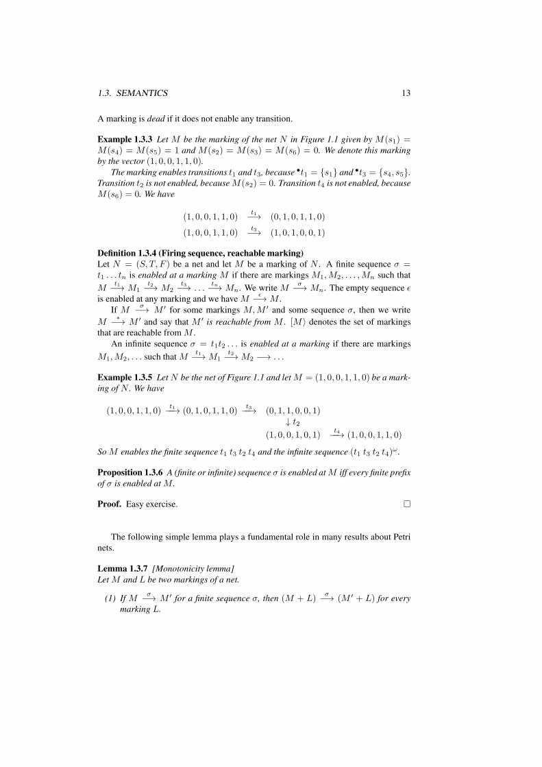
A marking is dead if it does not enable any transition.
Example 1.3.3 Let M be the marking of the net N in Figure 1.1 given by M(s1) =M(s4) = M(s5) = 1 and M(s2) = M(s3) = M(s6) = 0. We denote this marking
by the vector (1, 0, 0, 1, 1, 0).The marking enables transitions t1 and t3, because •t1 = {s1} and •t3 = {s4, s5}.
Transition t2 is not enabled, because M(s2) = 0. Transition t4 is not enabled, because
M(s6) = 0. We have
(1, 0, 0, 1, 1, 0)t1−→ (0, 1, 0, 1, 1, 0)
(1, 0, 0, 1, 1, 0)t3−→ (1, 0, 1, 0, 0, 1)
Definition 1.3.4 (Firing sequence, reachable marking)
Let N = (S, T, F ) be a net and let M be a marking of N . A finite sequence σ =t1 . . . tn is enabled at a marking M if there are markings M1,M2, . . . ,Mn such that
Mt1−→ M1
t2−→ M2t3−→ . . .
tn−→ Mn. We write Mσ−→ Mn. The empty sequence ǫ
is enabled at any marking and we have Mǫ−→M .
If Mσ−→ M ′ for some markings M,M ′ and some sequence σ, then we write
M∗−→ M ′ and say that M ′ is reachable from M . [M〉 denotes the set of markings
that are reachable from M .
An infinite sequence σ = t1t2 . . . is enabled at a marking if there are markings
M1,M2, . . . such that Mt1−→M1
t2−→M2 −→ . . .
Example 1.3.5 Let N be the net of Figure 1.1 and let M = (1, 0, 0, 1, 1, 0) be a mark-
ing of N . We have
(1, 0, 0, 1, 1, 0)t1−−→ (0, 1, 0, 1, 1, 0)
t3−−→ (0, 1, 1, 0, 0, 1)↓ t2
(1, 0, 0, 1, 0, 1)t4−−→ (1, 0, 0, 1, 1, 0)
So M enables the finite sequence t1 t3 t2 t4 and the infinite sequence (t1 t3 t2 t4)ω.
Proposition 1.3.6 A (finite or infinite) sequence σ is enabled at M iff every finite prefix
of σ is enabled at M .
Proof. Easy exercise. �
The following simple lemma plays a fundamental role in many results about Petri
nets.
Lemma 1.3.7 [Monotonicity lemma]
Let M and L be two markings of a net.
(1) If Mσ−→ M ′ for a finite sequence σ, then (M + L)
σ−→ (M ′ + L) for every
marking L.

14 CHAPTER 1. BASIC DEFINITIONS
(2) If Mσ−→ for an infinite sequence σ, then (M + L)
σ−→ for every marking L.
Proof. (1): by induction on the length of σ.
Basis: σ = ǫ. ǫ is enabled at any marking.
Step: Let σ = τt (t transition) such that Mτ−→ M ′′ t
−→ M ′. By induction hy-
pothesis (M + L)τ−→ (M ′′ + L). From the firing rule and M ′′ t
−→ M ′ we get
(M ′′ + L)t−→ (M ′ + L). So (M + L)
τt−→ (M ′ + L).
(2): We show that every finite prefix of σ is enabled at M +L. The result then follows
from Proposition 1.3.6. By Proposition 1.3.6, every finite prefix of σ is enabled at M .
That is, for every finite prefix τ of σ there is a marking M ′ such that Mτ−→ M ′. By
(1) we get (M + L)τ−→ (M ′ + L), and we are done. �
Definition 1.3.8 (Petri nets)
A Petri net, net system, or just a system is a pair (N,M0) where N is a connected net
N = (S, T, F ) with nonempty sets of places and transitions, and an initial marking
M0 : S → IN. A marking M is reachable in (N,M0) or a reachable marking of
(N,M0) if M0∗−→M .
Definition 1.3.9 (Reachability graph)
The reachability graph G of a Petri net (N,M0) where N = (S, T, F ) is the directed,
labeled graph satisfying:
• The nodes of G are the reachable markings of (N,M0).
• The edges of G are labeled with transitions from T .
• There is an edge from M to M ′ labeled by t iff Mt−→M , that is, iff M enables
t and the firing of t leads from M to M ′.
The algorithm of Figure 1.3 computes the reachability graph. It uses two functions:
• enabled(M): returns the set of transitions enabled at M .
• fire(M, t): returns the marking M ′ such that Mt−→M ′.
The set Work may be implemented as a stack, in which case the graph will be con-
structed in a depth-first manner, or as a queue for breadth-first. Breadth first search will
find the shortest transition path from the initial marking to a given (erroneous) marking.
Some applications require depth first search.

1.3. SEMANTICS 15
REACHABILITY-GRAPH((S, T, F,M0))1 (V,E, v0) := ({M0}, ∅,M0);2 Work : set := {M0};3 while Work 6= ∅4 do selectM from Work ;5 Work := Work \ {M};6 for t ∈ enabled(M)7 do M ′ := fire(M, t);8 if M ′ /∈ V9 then V := V ∪ {M ′}
10 Work := Work ∪ {M ′};11 E := E ∪ {(M, t,M ′)};12 return (V,E, v0)
Figure 1.3: Algorithm for computing the reachability graph

16 CHAPTER 1. BASIC DEFINITIONS
Chapter 2
Modelling with Petri nets
2.1 A buffer of capacity n
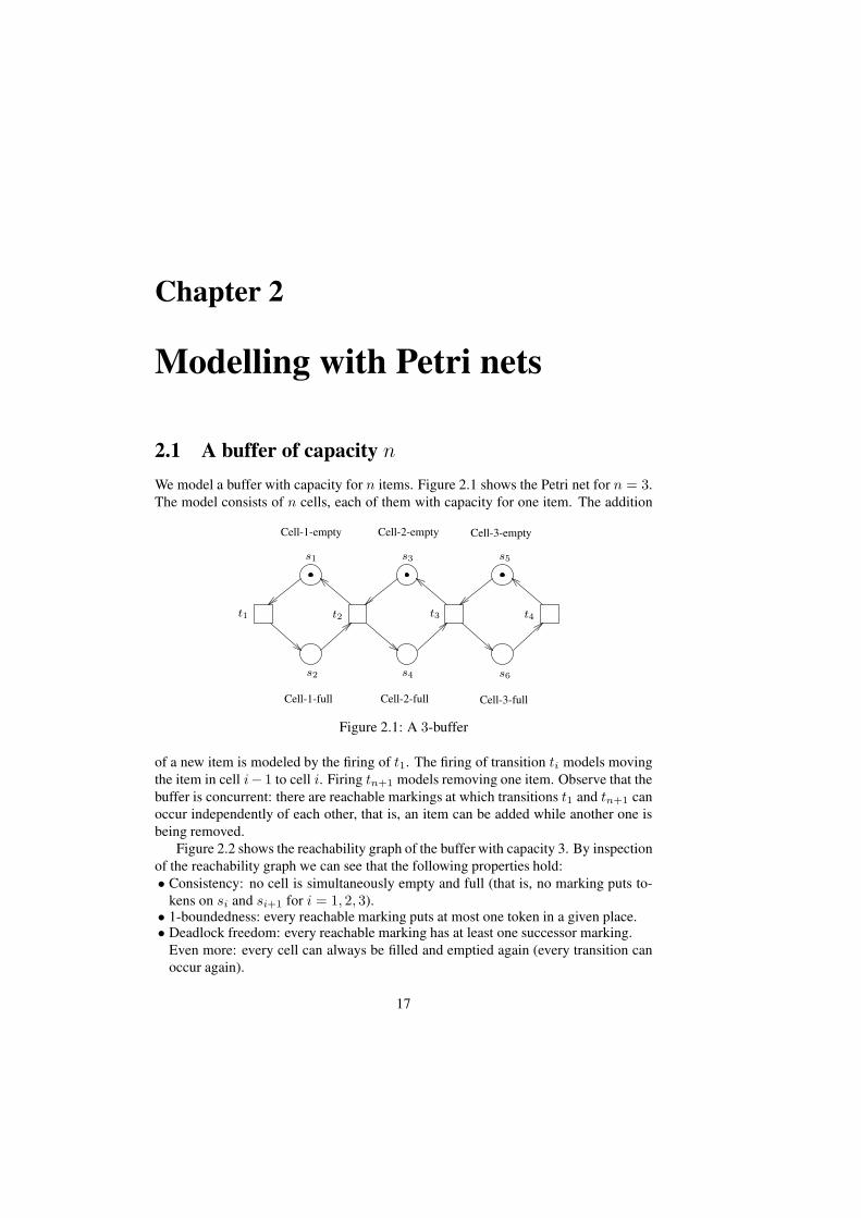
We model a buffer with capacity for n items. Figure 2.1 shows the Petri net for n = 3.
The model consists of n cells, each of them with capacity for one item. The addition
s1 s5
Cell-1-full Cell-2-full Cell-3-full
Cell-3-emptyCell-2-emptyCell-1-empty
t3t2t1
s6s4s2
t4
s3
Figure 2.1: A 3-buffer
of a new item is modeled by the firing of t1. The firing of transition ti models moving
the item in cell i− 1 to cell i. Firing tn+1 models removing one item. Observe that the
buffer is concurrent: there are reachable markings at which transitions t1 and tn+1 can
occur independently of each other, that is, an item can be added while another one is
being removed.
Figure 2.2 shows the reachability graph of the buffer with capacity 3. By inspection
of the reachability graph we can see that the following properties hold:
• Consistency: no cell is simultaneously empty and full (that is, no marking puts to-
kens on si and si+1 for i = 1, 2, 3).• 1-boundedness: every reachable marking puts at most one token in a given place.• Deadlock freedom: every reachable marking has at least one successor marking.
Even more: every cell can always be filled and emptied again (every transition can
occur again).
17

18 CHAPTER 2. MODELLING WITH PETRI NETS
(10 10)
10 10)
(10 10 10)
(01
01
10) (10 10
10
(10
(01 01 01)
(01 01)
01 01)
(01 01 01)
t2
t3
t1
t1t4
t1
t2
t4
t3t4
t1
t4
Figure 2.2: Reachability graph of the 3-buffer
• Capacity 3: the buffer has indeed capacity 3, that is, there is a reachable marking
that puts one token in s2, s4, s6.
• The initial marking is reachable from any reachable marking (that is, it is always
possible to empty the buffer).
• Between any two reachable markings there is a path of length at most 6.
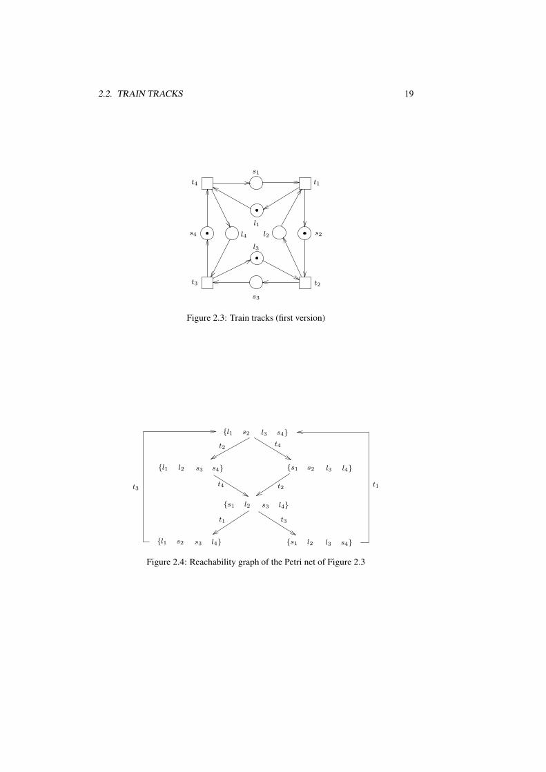
2.2 Train tracks
Four cities are connected by unidirectional train tracks building a circle. Two trains
circulate on the tracks. Our task is to ensure that it will never be the case that two trains
occupy the same track.
Figure 2.3 shows a solution of the problem modeled as a Petri net. the four tracks
are modeled by places s1, . . . , s4. A token on si means that there is train in the i-thtrack.
The four control places l1, . . . , l4 guarantee that no reachable marking puts more
than one token on si. This property can be proven by means of the reachability graph
shown in Figure 2.4. Since every reachable marking puts at most one token on a place,
we denote a marking by the set of places marked by it. For instance, we denote by
{l1, s2, l3, s4} the marking that puts a token on l1, s2, l3 and s4.
Consider now a slightly different system. We have 8 cities connected in a circuit,
and three trains use the tracks. To increase safety, we have to guarantee that there
2.2. TRAIN TRACKS 19
t1
s2
t2t3
s4
t4
s1
l3
l1
s3
l4 l2
Figure 2.3: Train tracks (first version)
s2 l3
s2 l3
s2 l3
l2 s3
l2 s3
s3 l2
t3
t4
t4
t3t1
t1
t2
t2
{l1 s4}
{l1 s4} {s1 l4}
{s1 l4}
{l1 l4} {s1 s4}
Figure 2.4: Reachability graph of the Petri net of Figure 2.3

20 CHAPTER 2. MODELLING WITH PETRI NETS
Figure 2.5: Train tracks (second version)
always is at least one empty track between any two trains.
The Petri net of Figure 2.5 is a solution of the problem: The reader can construct
the reachability graph and show that the desired property holds. However, the graph is
pretty large!
2.3 Dining philosophers
Four philosophers sit around a round table. There are forks on the table, one between
each pair of philosophers. The philosophers want to eat spaghetti from a large bowl
in the center of the table (see the top of Figure 2.6). Unfortunately the spaghetti is
of a particularly slippery type, and a philosopher needs both forks in order to eat it.
The philosophers have agreed on the following protocol to obtain the forks: Initially
philosophers think about philosophy, when they get hungry they do the following: (1)
take the left fork, (2) take the right fork and start eating, (3) return both forks simul-
taneously, and repeat from the beginning. Figure 2.6 shows a Petri net model of the
system.
Two interesting questions about this systems are:
• Can the philosophers starve to death (because the system reaches a deadlock)?
• Will an individual philosopher eventually eat, assuming she wants to?
2.4 A logical puzzle
A man is travelling with a wolf, a goat, and a cabbage. The four come to a river that
they must cross. There is a boat available for crossing the river, but it can carry only
the man and at most one other object. The wolf may eat the goat when the man is not
around, and the goat may eat the cabbage when unattended (see Figure 2.7)

2.4. A LOGICAL PUZZLE 21
4
1 2
3
fork
fork
fork fork
l1 ✛✠
❄r1✲ ✲
✻
b1
✻
✛
❘
■
thinking
eating
r2✛❘
✻
l2✲ ✲
✻
b2
❄
✛
✠
✒
eating
thinking
l3✲
✒
✻
r3✛ ✛❄
b3❄
✲
■
❘
thinking
eating
r4 ✲
■
❄
l4✛ ✛❄
b4
✻
✲
✒
✠
eating
thinking
Figure 2.6: Petri net model of the dining philosophers
22 CHAPTER 2. MODELLING WITH PETRI NETS
Can the man bring everyone across the river without endangering the goat or the
cabbage? And if so, how?
We model the system with a Petri net. The puzzle mentions the following objects:
Man, wolf, goat, cabbage, boat. Both can be on either side of the river. It also mentions
the following actions: Crossing the river, wolf eats goat, goat eats cabbage.
Objects and their states are modeled by places. (We can omit the boat, because it is
always going to be on the same side as the man.) Actions are modeled by transitions.
Figure 2.7 shows the transitions for the three actions.
2.5 Peterson’s algorithm
Peterson’s algorithm is a well-known solution to the mutual exclusion problem for two
processes.
var m1,m2 : {false, true} (init false);
hold : {1, 2};
while true do
m1 := true;hold := 1;await(¬m2 ∨ hold = 2);(critical section);
m1 := false;od
while true do
m2 := true;hold := 2;await(¬m1 ∨ hold = 1);(critical section);
m2 := false;od
The Petri net of Figure 2.8 models this algorithm. The variable mi is modeled by
the places mi = true and mi = false . A token on mi = true means that at the
current state of the program (marking) the variable mi has the value true (so the Petri
net must satisfy the property that no reachable marking puts tokens on both mi = true
and mi = false at the same time). Variable hold is modeled analogously.
A token on p4 (q4) indicates that the left (right) process is in its critical section.
Mutual exclusion holds if no reachable marking puts a token on p4 and q4. The Petri
net has 20 reachable markings.
2.6 The action/reaction protocol
Two agents must repeatedly exchange informations. When an agent requests an infor-
mation from the other one, it must wait for an answer before proceeding. The task is to
design a protocol for the exchanges. In particular, the protocol must guarantee that it
is not possible to reach a situation in which both processes are waiting from an answer
from the other one.
A first attempt at a solution is shown in Figure 2.9. Requests are modeled by the
Action transitions, and replies by the Reaction transitions. However, this solution can
reach a deadlock: both processes can issue a request simultaneously, after which they

2.6. THE ACTION/REACTION PROTOCOL 23
Man
Wolf
Goat
Cabbage
Left bank
CL
GL
WL
ML
Right bank
Wolf
Goat
Cabbage
ManMR
WR
GR
CR
WLR
MLR
CLR
GLR
Man
Wolf
Goat
Cabbage
Left bank
CL
GL
WL
ML
Right bank
Wolf
Goat
Cabbage
ManMR
WR
GR
CR
WRL
MRL
CRL
GRL
Man
Wolf
Goat
Cabbage
Left bank
CL
GL
Right bank
Wolf
Goat
Cabbage
ManMR
WR
GR
CR
WL
ML
WGL WGR
CGL CGR
Figure 2.7: Transitions modelling the actions of the puzzle

24 CHAPTER 2. MODELLING WITH PETRI NETS
q4
q3
v1
v4
v3
q2
v6
q1
u1u6
u3
u4
m1 = t
m2 = fp1
p2
p3
p4
hold = 2
m2 = t
u5
hold = 1
v5
u2 v2
m1 = f
Figure 2.8: Petri net model of Peterson’s algorithm
wait forever for an answer. We call such a situation a crosstalk. Figure 2.10 shows a
second attempt. Now processes can detect that a crosstalk has taken place. If a process
detects a crosstalk, it answers the request of its partner, and then continues to wait for an
answer to its own request. This solution has no deadlocks (prove it!), but it exhibits the
following problem: a non-cooperative process can always get answers to its requests,
without ever answering any request from its partner. The solution is deadlock free, but
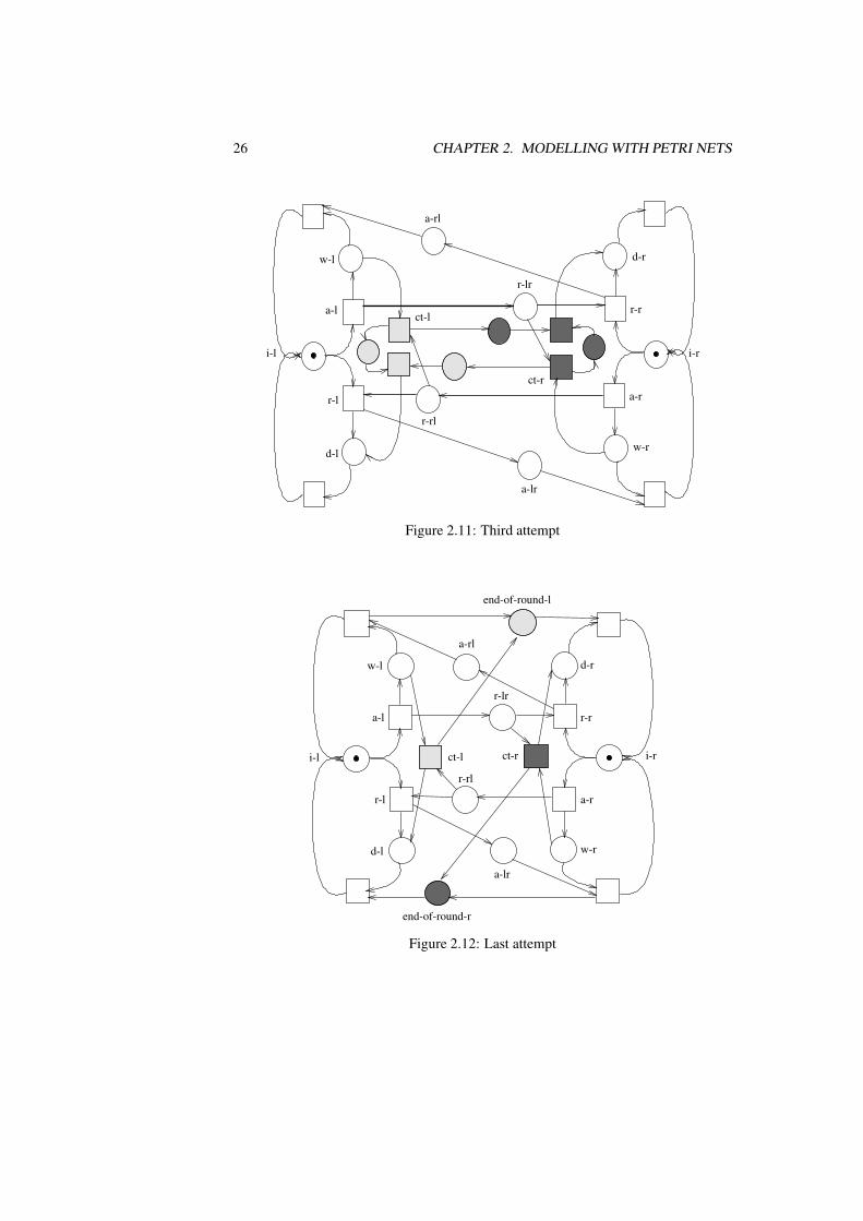
unfair. The third attempt (Figure 2.11) is fair. If a process detects a crosstalk, then it
answers the request of its partner, as before, but then it moves to a state in which it is
only willing to receive an answer to its own question. Unfortunately, the system has
again a deadlock (can you find it?).
The final attempt (Figure 2.12) is both deadlock-free and fair. The protocol works
in rounds. A “good” round consists of a request and an answer. In a “bad” round both
processes issue a request and they reach a crosstalk situation. Such a round continues as
follows: both processes detect the crosstalk, send each other an “end-of-round” signal,
wait for the same signal from their partner, and then move to their initial states.
The solution is not perfect. In the worst case there are only bad rounds, and no
requests are answered at all.
2.7 Variants of the main model
Definition 2.7.1 (Nets with place capacities)
A net with capacities N = (S, T, F,K) consists of a net (S, T, F ) and a mapping
K : S → IN.
A transition t is enabled at a marking M of N if

2.7. VARIANTS OF THE MAIN MODEL 25
wait-l
action-l
reaction-l
answer-rl
request-rl
request-lr
reaction-r
done-r
action-r
wait-r
answer-lr
done-l
idle-l idle-r
Figure 2.9: First attempt
ct-rct-l i-r
r-r
d-r
a-r
w-rd-l
r-l
i-l
a-l
w-l
a-rl
r-lr
r-rl
a-lr
Figure 2.10: Second attempt
26 CHAPTER 2. MODELLING WITH PETRI NETS
ct-l
ct-r
i-l
a-l
w-l
r-l
d-l
i-r
a-rl
a-lr
r-lr
r-rl
d-r
r-r
a-r
w-r
Figure 2.11: Third attempt
end-of-round-l
end-of-round-r
i-r
r-l
i-l
a-l
w-r
d-r
r-r
a-r
w-l
d-l
r-lr
ct-l ct-r
a-lr
r-rl
a-rl
Figure 2.12: Last attempt

2.7. VARIANTS OF THE MAIN MODEL 27
Ri Si
ri
si
m
m
wj
Vj
vj
m
Wj
Ri: Process i reads
Process i idleSi:
ri: Process i starts reading
si: Process i stops reading
Wi:
Vj :
Process j writes
Process j idle
wj : Process j starts writing
vj : Process j stops writing
m readers n writers
Figure 2.13: Readers and writers
– M(s) ≥ 1 for every place s ∈ •t and
– M(s) < K(s) for every place s ∈ t• \ •tThe notions of firing, Petri net with capacities, etc. are defined as in the capacity-free
case.
Definition 2.7.2 (Nets with weighted arcs)
A net with weighted arcs N = (S, T,W ) consists of two disjoint sets of places and
transitions and a weight function W : (S×T )∪(T×S)→ IN. A transition t is enabled
at a marking M of N if M(s) ≥ W (s, t) for every s ∈ S. If t is enabled then it can
occur leading to the marking M ′ defined by
M ′(s) = M(s) +W (t, s)−W (s, t)
for every place s. Other notions are defined as in the standard model.
The Petri net with weighted arcs of Figure 2.13 models a solution to the “readers
and writers” problem. A set of processes has access to a database. Processes can read
concurrently, but a process can only write if no other processes reads nor writes.
Exercise: Modify the Petri net so that reading processes can not indefinitely pre-
vent another process from writing.
Definition 2.7.3 (Nets with inhibitor arcs)
A net with inhibitor arcs N = (S, T, F, I) consists of two disjoint sets of places and
transitions, a set F ⊆ (S×T )∪ (T ×S) of arcs, and a set I ⊆ S×T , disjoint with F ,
of inhibitor arcs. A transition t is enabled at a marking M of N if M(s) > 0 for every

28 CHAPTER 2. MODELLING WITH PETRI NETS
place s such that (s, t) ∈ F , and M(s) = 0 for every place s such that (s, t) ∈ I . If
t is enabled then it can occur leading to the marking M ′, defined as for standard Petri
nets.
Definition 2.7.4 (Nets with reset arcs)
A net with reset arcs N = (S, T, F,R) consists of two disjoint sets of places and
transitions, a set F ⊆ (S × T ) ∪ (T × S) of arcs, and a set R ⊆ S × T , disjoint with
F , of reset arcs. A transition t is enabled at a marking M of N if M(s) > 0 for every
place s such that (s, t) ∈ F ∪R. If t is enabled then it can occur leading to the marking
obtained after the following operations:
• Remove one token from every place s such that (s, t) ∈ F .
• Remove all tokens from every place s such that (s, t) ∈ R.
• Add one token to every place s such that (t, s) ∈ F .
2.8 Analysis problems
We introduce a number of properties we are interested in. We assume that nets have at
least one place and one transition.
Definition 2.8.1 (System properties)
Let (N,M0) be a Petri net.
(N,M0) is deadlock free if every reachable marking enables at least one transition
(that is, no reachable marking is dead).
(N,M0) is live if for every reachable marking M and every transition t there is a
marking M ′ ∈ [M〉 that enables t. (Intuitively: every transition can always fire again).
(N,M0) is bounded, if for every place s there is a number b ≥ 0 such that
M(s) ≤ b for every reachable marking M . M0 is a bounded marking of N if (N,M0)is bounded. The bound of a place s of a bounded Petri net (N,M0) is the number
max{M(s) |M ∈ [M0〉}
(N,M0) is b-bounded if every place has bound b.
In these notes we study the following problems:
• Deadlock freedom: is a given Petri net (N,M0) deadlock-free?
• Liveness: is a given Petri net (N,M0) live?
• Boundedness: is a given Petri net (N,M0) bounded?
• b-boundedness: given b ∈ N and a Petri net (N,M0), is (N,M0) b-bounded?
• Reachability: given a Petri net (N,M0) and a markingM ofN , is M reachable?
• Coverability: given a Petri net (N,M0) and a marking M of N , is there a
reachable marking M ′ ≥M?

2.8. ANALYSIS PROBLEMS 29
There are some simple connections between these problems:
Proposition 2.8.2
(1) Liveness implies deadlock freedom.
(2) If (N,M0) is bounded then there is a number b such that (N,M0) is b-bounded.
(3) If (N,M0) is bounded, then it has finitely many reachable markings.
Proof. (1) follows immediately from the definitions. (2) and (3) follow from the defi-
nitions and from the fact that a Petri net has finitely many places. �
Sometimes we also use the following notion
Definition 2.8.3 (Well-formed nets)
A net N is well formed if there is a marking M0 such that the Petri net (N,M0) is live
and bounded.
and consider the following problem
• Well-formedness: is a given net well formed?

30 CHAPTER 2. MODELLING WITH PETRI NETS
Part II
Analysis Techniques for Petri
Nets
31


33
Chapter 3 shows (sometimes without proofs) that Deadlock-freedom, Liveness,
Boundedness, b-Boundedness, Coverability, and Reachability are all decidable. The
decision procedures for these problems have high complexity, but, at the same time,
results of complexity theory show that no efficient algorithms exist for them.
Since better runtimes are often required in many practical applications, we often
use algorithms that can be applied to arbitrary Petri nets, but sometimes answer “don’t
know”, or do not terminate. We call them semi-decision procedures. We also use faster
decision procedures for special Petri net classes.
Chapter 4 is devoted to semi-decision procedures. Chapter 5 presents efficient de-
cision algorithms for three classes: S-nets, T -nets, and Free-Choice nets

34

Chapter 3
Decision procedures
3.1 A decision procedure for Boundedness
The b-Boundednesss problem is clearly decidable: if the input Petri net (N,M0) has
n places, then the number of b-bounded markings of N is nb+1. So we can decide
b-Boundedness by constructing the reachability graph of (N,M0) until either the con-
struction terminates, or we find a reachable marking that is not b-bounded.
The same idea gives a semi-decision procedure for Boundedness: again, we con-
struct the reachability graph. If the input (N,M0) is bounded, then there are finitely
many reachable markings, the construction terminates, and we can return “bounded”.
However, if the net is unbounded then this procedure does not terminate.
We now give a decision procedure for Boundedeness. We need two lemmas. The
first one is a simple adaptation of Konig’s Lemma; the second is known as Dickson’s
Lemma.
Lemma 3.1.1 (Konigs lemma) Let G = (V,E) be the reachability graph of a Petri
net (N,M0). If V is infinite, then G contains an infinite simple path.
Proof. Assume V = [M0〉 is infinite. For every reachable marking M there is a
simple path πM from M0 to M . Since M0 has finitely many immediate successors
(at most one for each transition of N ), and each πM visits one of them, at least one
immediate successor M1 of M0 has infinitely many successors in (V \ {M0}, E), that
is, [M1〉 \ {M0} is infinite. Iterating this argument we construct an infinite simple path
M0M1M2 · · · . �
Lemma 3.1.2 (Dickson’s lemma) For every infinite sequence A1A2A3 . . . of vectors
of Nk there is an infinite sequence i1 < i2 < i3 . . . of indices such that Ai1 ≤ Ai2 ≤Ai3 . . ..
Proof. By induction on kBasis: k = 1. Then the elements of A are just numbers. The set {A1, A2, · · · } has
35
36 CHAPTER 3. DECISION PROCEDURES
a minimum, say c1. Choose i1 as some index (say, the smallest), such that Ai1 = c1.
Consider now the set {Ai1+1, Ai1+2, · · · }. The set has a minimum c2, which by defi-
nition satisfies c1 ≤ c2. Choose i2 as the the smallest index i2 > i1 such that Ai2 = c2.
Etc.
Step: k > 1. Given a vector Ai, let A′i be the vector of dimension k − 1 consisting
of the first k − 1 components of Ai, and let ai be the last component of Ai. We write
Ai = (A′i | ai).
Since the vectors of A′1A
′2A
′3 · · · have dimension k − 1, by induction hypothesis
there is an infinite subsequence A′i1≤ A′
i2≤ A′
i3· · · . Consider now the sequence
ai1ai2ai3 · · · . By induction hypothesis there is a subsequence aj1 ≤ aj2 ≤ aj3 · · · .But then we have Aj1 ≤ Aj2 ≤ Aj3 · · · , and we are done. �
Remark: Lemma 3.1.2 shows that the partial order≤⊆ Nk×Nk is a well-quasi-order.
Given a set A, and a partial order �⊆ A × A, we say that � is a well-quasi-order if
every infinite sequence a1a2a3 · · · ∈ Aω contains an infinite chain ai1 � ai2 � · · · . In
the next section we examine well-quasi-orders in more detail.
We use Konig’s Lemma and Dickson’s lemma to provide the following characteri-
zation of unboundedness.
Theorem 3.1.3 (N,M0) is unbounded iff there are markings M and L such that L 6=
0 and M0∗−→M
∗−→ (M + L)
Proof. (⇐) : Assume there are such markings M,L. By the Monotonicity Lemma we
have
M1∗−→ (M1 + L)
∗−→ (M1 + 2 · L)
∗−→ . . .
So the set [M0〉 of reachable markings is infinite and (N,M0) is unbounded.
(⇒) Assume (N,M0) is unbounded. Then the set [M0〉 of reachable markings is in-
finite. By Konigs lemma there is an infinite firing sequence M0t1−→ M1
t1−→ M2 . . .that never visits a marking twice. By Dickson’s Lemma there are Mi and Mj such that
M0∗−→Mi
∗−→Mj and Mi ≤Mj . Let M ≡Mi and L ≡Mj −Mi. �
Theorem 3.1.4 Boundedness is decidable.
Proof. We give an algorithm that always terminates and always returns the correct
answer: “ bounded” or “unbounded”. The algorithm explores the reachability graph
of the net using breadth-first search. After adding a new marking M ′, the algorithm
checks if the part of the graph already constructed contains a sequence M0∗−→M
∗−→
M ′ such that M ≤ M ′ (and M 6= M ′, because M ′ is new). The algorithm terminates
if it finds such a sequence, in which case it returns “unbounded”, or if it cannot add any
new marking, in which case it returns “bounded”.
If (N,M0) is bounded, then by Theorem 3.1.3 the algorithm never finds a new
marking M ′ satisfying the condition above. So, since the Petri net has only finitely

3.2. DECISION PROCEDURES FOR COVERABILITY 37
many reachable markings, the algorithm terminates because it cannot find any new
marking, and correctly returns “bounded”.
If (N,M0) is unbounded, then there are infinitely many reachable markings, and
the algorithm cannot terminate because it runs out of reachable markings. On the other
hand, by Theorem 3.1.3 the algorithm eventually finds markings M ′ and M as above,
and so it correctly answers “unbounded”. �
3.2 Decision procedures for Coverability
The reachability graph of a Petri net can be infinite, in which case the algorithm for
computing the reachability graph will not terminate. Therefore, the algorithm cannot
decide that a given marking is not coverable. In this section we introduce several
decision procedures that overcome this problem.
3.2.1 Coverability graphs
We show how to construct a coverability graph of a Petri net (N,M0). The coverability
graph is always finite, and satisfies the following property: a marking M of (N,M0)is coverable iff some node M ′ of the coverability graph of (N,M0) covers M , i.e.,
satisfies M ′ ≥M .
We introduce a new symbol ω. Intuitively, it stands for an arbitrarily large number.
We extend the arithmetic on natural numbers with ω as follows. For all n ∈ N:
n+ ω = ω + n = ω,
ω + ω = ω,
ω − n = ω,
0 · ω = 0n ≥ 1⇒ n · ω = ω · n = ω,
n ≤ ω and ω ≤ ω.
Observe that ω − ω remains undefined, but we will not need it.
We extend the notion of markings to ω-markings. An ω-marking of a net N =(S, T, F ) is a mapping M : S → N ∪ {ω}. Intuitively, in an ω-marking, each place shas either a certain number of tokens or “arbitrarily many” tokens.
The enabledness condition and the firing rule neatly extend to ω-markings with
the extended arithmetic rules: recall that a transition t is enabled at a marking M if
M(s) > 0 for every s ∈ •t. Now M(s) > 0 may hold because M(s) = ω. Further,
recall that if t is enabled, then it can fire, leading from M to the marking M ′ given by:
M ′(s) =
M(s)− 1 if s ∈ •t \ t•
M(s) + 1 if s ∈ t• \ •tM(s) otherwise
If s ∈ •t ∪ t• and M(s) = ω, then we have M ′(s) = ω. That is, if a place contains
ω tokens, then firing a transition will not change its number of tokens, even if the
transition is connected with an arc to the place.
38 CHAPTER 3. DECISION PROCEDURES
M t1 t2 ... tn M’ t1 t2 ... tn M’’= =
∆Μ ∆ΜΜ+∆Μ Μ+2∆Μ
...
=...
Figure 3.1: Pumping tokens.
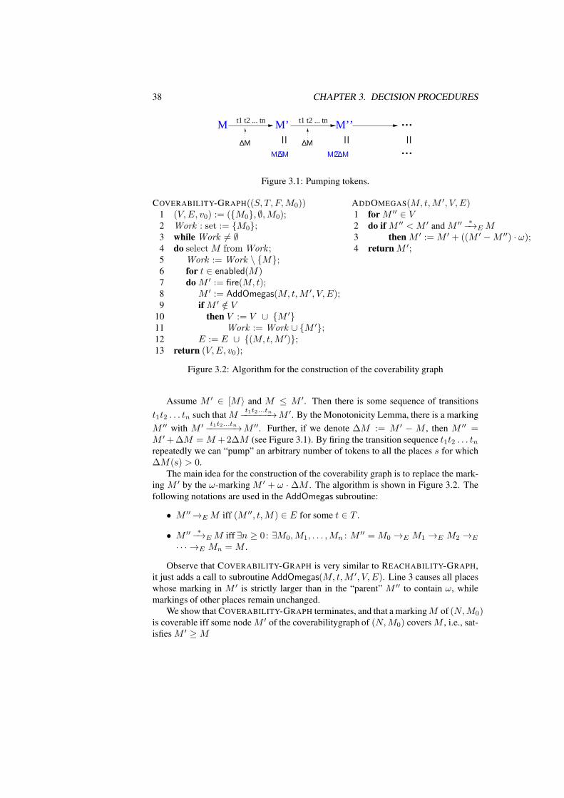
COVERABILITY-GRAPH((S, T, F,M0))1 (V,E, v0) := ({M0}, ∅,M0);2 Work : set := {M0};3 while Work 6= ∅4 do select M fromWork ;5 Work := Work \ {M};6 for t ∈ enabled(M)7 do M ′ := fire(M, t);8 M ′ := AddOmegas(M, t,M ′, V, E);9 if M ′ /∈ V
10 then V := V ∪ {M ′}11 Work := Work ∪ {M ′};12 E := E ∪ {(M, t,M ′)};13 return (V,E, v0);
ADDOMEGAS(M, t,M ′, V, E)1 for M ′′ ∈ V2 do if M ′′ < M ′ and M ′′ ∗
−→E M3 then M ′ := M ′ + ((M ′ −M ′′) · ω);4 return M ′;
Figure 3.2: Algorithm for the construction of the coverability graph
Assume M ′ ∈ [M〉 and M ≤ M ′. Then there is some sequence of transitions
t1t2 . . . tn such that Mt1t2...tn−−−−−−→M ′. By the Monotonicity Lemma, there is a marking
M ′′ with M ′ t1t2...tn−−−−−−→M ′′. Further, if we denote ∆M := M ′ − M , then M ′′ =M ′+∆M = M +2∆M (see Figure 3.1). By firing the transition sequence t1t2 . . . tnrepeatedly we can “pump” an arbitrary number of tokens to all the places s for which
∆M(s) > 0.
The main idea for the construction of the coverability graph is to replace the mark-
ing M ′ by the ω-marking M ′ + ω · ∆M . The algorithm is shown in Figure 3.2. The
following notations are used in the AddOmegas subroutine:
• M ′′−→E M iff (M ′′, t,M) ∈ E for some t ∈ T .
• M ′′ ∗−→E M iff ∃n ≥ 0: ∃M0,M1, . . . ,Mn : M
′′ = M0 →E M1 →E M2 →E
· · · →E Mn = M .
Observe that COVERABILITY-GRAPH is very similar to REACHABILITY-GRAPH,
it just adds a call to subroutine AddOmegas(M, t,M ′, V, E). Line 3 causes all places
whose marking in M ′ is strictly larger than in the “parent” M ′′ to contain ω, while
markings of other places remain unchanged.
We show that COVERABILITY-GRAPH terminates, and that a markingM of (N,M0)is coverable iff some node M ′ of the coverabilitygraph of (N,M0) covers M , i.e., sat-
isfies M ′ ≥M

3.2. DECISION PROCEDURES FOR COVERABILITY 39
Theorem 3.2.1 COVERABILITY-GRAPH terminates.
Proof. Assume that COVERABILITY-GRAPH does not terminate. We derive a con-
tradiction. If COVERABILITY-GRAPH does not terminate, then it constructs an infinite
graph. Since every node of the graph has at most |T | successors, by Konig’s lemma
the graph contains an infinite path Π = M1M2 . . .. If an ω-marking Mi of Π satisfies
Mi(p) = ω for some place p, then Mi+1(p) = Mi+2(p) = . . . = ω. So Π con-
tains a marking Mj such that all markings Mj+1,Mj+2, . . . have ω’s at exactly the
same places as Mj . Let Π′ be the suffix of Π starting at Mj . Consider the projection
Π′′ = mjmj+1 . . . of Π′ onto the non-ω places. Let n be the number of non-ω places.
Π′′ is an infinite sequence of distinctn-tuples of natural numbers. By Dickson’s lemma,
this sequence contains markings Mk,Ml such that k < l and Mk ≤Ml. This is a con-
tradiction, because, since Mk 6= Ml, when executing AddOmegas(Ml−1, t,Ml, V, E)the algorithm adds at least one ω to Ml−1. �
For the rest of the proof we start with a lemma.
Lemma 3.2.2 For every ω-marking M ′ added by the algorithm to V and for every
k > 0, there there is a reachable marking M ′k satisfying M ′
k(s) = M ′(s) for every
place s such that M ′(s) ∈ N, and M ′k(s) > k for every place s such that M ′(s) = ω.
Proof. We prove that if all ω-markings added so far to V satisfy the property, then the
next one also does. Assume the algorithm currently explores markingM and transition
t, and let Mt−→M1. By induction hypothesis, for every k > 0, there there is a reach-
able markingMk satisfying Mk(s) = M(s) for every place s such that M(s) ∈ N, and
Mk(s) > k for every place s such that M(s) = ω. If AddOmegas does not add any
ωs, then we can take M ′k as the result of firing t from Mk. Assume AddOmegas finds
an ω-marking M ′′ such that M ′′ ∗−→E M
t−→M1. Then there is a sequence σ such that
M ′′ σ−→M
t−→M1. By induction hypothesis, for every k > 0, there is a reachable
marking M ′′k satisfying M ′′
k (s) = M ′′(s) for every place s such that M ′′(s) ∈ N, and
M ′′k (s) > k for every place s such that M ′′(s) = ω. Then, starting from a sufficiently
large k, the marking M ′′k enables σt (for instance, take k = |σt|, since a σt can remove
at most |σt| tokens from a place). We can then choose Mk as the marking satisfying
M ′′k
σt−−→M ′
k.
If AddOmegas finds several ω-markings M ′′ such that M ′′ ∗−→E M
t−→M1, we re-
peat the argument above. �
Theorem 3.2.3 Let (N,M0) be a Petri net and let M be a marking of N . There is
a reachable marking M ′ ≥ M iff the coverability graph of (N,M0) contains an ω-
marking M ′′ ≥M .
Proof. (⇒): Assume there is a reachable marking M ′ ≥ M . Then some firing
sequence
M0t1−−→M1
t2−−→M2 · · ·Mn−1tn−−→M ′

40 CHAPTER 3. DECISION PROCEDURES
of (N,M0) leads from M0 to M ′. By the definition of the algorithm, the coverability
graph contains a path
M0t1−−→M ′
1t2−−→M ′
2 · · ·M′n−1
tn−−→M ′n
such that M ′i ≥Mi for every 1 ≤ i ≤ n. Take M ′′ = M ′
n.
(⇐): Assume the coverability graph of (N,M0) contains an ω-marking M ′′ ≥M .
By Lemma 3.2.2, there is a reachable marking M ′′k satisfying M ′′
k (s) = M ′′(s) for
every place s such that M ′′(s) ∈ N, and M ′′k (s) > k for every place s such that
M ′′(s) = ω. Take k larger than any of the components of M , and set M ′ = M ′′k . Then
clearly M ′ ≥M . �
Size of the coverability graph
Let Bn be the set of bounded Petri nets with k places {s1, . . . , sk} and an initial mark-
ing putting only one token on s1 and zero tokens elsewhere (observe that Bn is essen-
tially finite, because the maximal number of transitions with different presets of post-
sets is 22k). It has been proved that the function giving for each n ≥ 1 the maximal
size of the reachability graph of the nets in Bn is not bounded by any primitive re-
cursive function. Since for bounded Petri nets the reachability and coverability graphs
coincide, the same result holds for the coverability graphs.
3.2.2 Rackoff’s theorem
The coverability graph allows us to answer coverability of any marking. However,
Coverability asks whether a particular marking M can be covered. The question is
whether we can give a bound on the size of the fragment of the coverability graph we
need to construct to find an ω-marking covering M .
Definition 3.2.4 (Integer nets) Let N = (S, T, F ) be a net. A generalized marking
of N (g-marking for short) is a mapping G : S → Z. An integer net is a pair (N,G0)where N is a net and G0 is a g-marking. A g-marking G enables all transitions, and
the occurrence of t at G leads to the marking G′ given by
G′(s) =
G(s)− 1 if s ∈ •t \ t•
G(s) + 1 if s ∈ t• \ •tG(s) otherwise
We denote by Gt→ G′ that firing t at G yields to G′.
An integer firing sequence of an integer net is a sequenceG0t1→ G1
t2→ · · ·
tn→ Gm.
Clearly, every Petri net is also an integer net, and every firing squence is also an
integer firing sequence, but the converse does not hold.
In the rest for the section we fix a net N with places {s1, . . . , sk}, and identify
g-markings with vectors of Zk .

3.2. DECISION PROCEDURES FOR COVERABILITY 41
Definition 3.2.5 Let G ∈ Zk be a g-marking of N and let 0 ≤ i ≤ k. We say that
G is i-natural if its first i-components are natural numbers, i.e., if G(j) ≥ 0 for every
1 ≤ j ≤ i. If moreover G(j) < r for every 1 ≤ j ≤ i, then we say that G is
(i, r)-natural.
An integer sequence σ = G0t1→ · · ·
tm→ Gm is i-natural (respectively (i, r)-
natural) if every generalized marking of σ is i-natural (respectively (i, r)-natural).
Given a g-marking G ∈ Zk, we say that σ is (i, G)-covering if Gm(j) ≥ G(j) for
every 1 ≤ j ≤ i.
Intuitively, G is i-natural if its restriction to the first i places is a “normal” marking,
and σ is i-natural if its restriction to the first i places is a “normal” firing sequence.
So, in particular, deciding if M is coverable in a Petri net (N,M0) with k places is
equivalent to deciding if (N,M0) has a (k,M)-covering and k-natural sequence.
We prove the following result:
Theorem 3.2.6 Let n = max(1, |G(1)|, . . . |G(k)|). For every G0 ∈ Zk, if (N,G0)has a (k,G)-covering, k-natural sequence, then it has one of length at most (n +
1)(2k)k
.
This upper bound is not very precise. The only important aspect is the double
exponential dependency on k, the number of places of the net. The proof follows
easily from the following lemma, which gives a tighter bound, but in the form of a
recursively defined function:
Lemma 3.2.7 For every G0 ∈ Zk and for every 1 ≤ i ≤ k, if (N,G0) has an (i, G)-covering, i-natural sequence, then it has one of length at most f(i), where f is induc-
tively defined as follows:
• f(0) = 1, and
• f(i) = (nf(i− 1))i + f(i− 1) for every 1 ≤ i ≤ k.
Proof The proof is by induction on i.Base: i = 0. Follows from the fact that the sequence σ = G0 is (0, G)-covering and
0-natural.
Step: i > 0. Assume (N,G0) has an (i, G)-covering, i-natural sequence. We consider
two cases:
Case 1: (N,G0) has an (i, G)-covering, (i, nf(i− 1))-natural sequence.
Assume the sequence is
σ = G0t1→ · · ·
tm→ Gm
and assume further that it has minimal length.
We claim that G0, G1, . . . , Gm are pairwise different in the first i places. Assume
the contrary: there exist α < β such that Gα(j) = Gβ(j) for every 1 ≤ j ≤ i. Then
the sequence
σ′ = G0t1→ · · ·
tα−1
−−−−→Gα
tβ+1
→ G′β+1
tβ+2
→ · · ·tm→ G′
m

42 CHAPTER 3. DECISION PROCEDURES
is also (i, G)-covering and (i, nf(i − 1))-natural, contradicting the minimality of σ.
This proves the claim.
Since σ is (i, nf(i − 1))-natural, for every g-marking G′ appearing in σ we have
0 ≤ G′(j) < nf(i−1) for every 1 ≤ j ≤ i. There are at most (nf(i−1))i g-markings
G′ different in the first i places satisfying 0 ≤ G′(j) < nf(i− 1). By the claim above
the length of σ is at most (nf(i− 1))i.
Case 2: (N,G0) has no (i, G)-covering, (i, nf(i− 1))-natural sequence.
Then there is an (i, G)-covering, i-natural sequence that is not (i, nf(i − 1))-natural.
Let this sequence be
σ = G0t1→ G1
t2→ · · ·Gm−1
tm→ Gm
Let Gα+1 be the first vector of σ that is not (i, nf(i − 1))-natural. Without loss of
generality, we can assume Gα+1(i) ≥ nf(i− 1). Then the prefix
G0t1→ · · ·
tα→ Gα
is (i, Gα)-covering and (i, nf(i− 1))-natural. As in the previous case, we can assume
α ≤ (nf(i− 1))i.
Since
Gα+1
tα+1
→ · · ·tm→ Gm
is an (i − 1, G)-covering and (i − 1)-natural sequence of (N,Gα+1), by induction
hypothesis there exists another (i − 1, G)-covering and (i− 1)-natural sequence
Gα+1u1
→ H1u2
→ · · ·uℓ→ Hℓ
of (N,Gα+1) of length at most f(i−1), that is, ℓ ≤ f(i−1). Since Gα+1(i) ≥ nf(i−1), and a sequence of length f(i − 1) can remove at most (f(i − 1)− 1) tokens from
the place si, after the execution of the new sequence we still have Hℓ(si) ≥ n ≥ G(si)and Hℓ(si) ≥ 0. So the sequence
σ′ = G0t1→ · · ·
tα→ Gα
tα+1
→ Gα+1u1
→ H1u2
→ · · ·uℓ
→ Hℓ
is an (i, G)-covering and i-natural sequence of (N,G0) of length at most (nf(i−1))i+f(i− 1). �
We can now proceed to prove Theorem 3.2.6:
Proof of Theorem 3.2.6. Define g(0) = n + 1 and g(i) = (g(i − 1))2k for every
1 ≤ i ≤ k. Observe that g(i) ≥ n+ 1 for every i ≥ 0. We prove f(i) ≤ g(i) for every
0 ≤ i ≤ k by induction on i. For i = 0 we have f(0) = 1 ≤ n = g(0). For i > 0 we

3.2. DECISION PROCEDURES FOR COVERABILITY 43
have
f(i) = (nf(i− 1))i + f(i− 1)
≤ (ng(i− 1))k + g(i− 1)
≤ (ng(i− 1))k + g(i− 1)k
= (nk + 1)g(i− 1)k
≤ (n+ 1)kg(i− 1)k
≤ g(i− 1)kg(i− 1)k
= g(i)
By Lemma 3.2.7, if (N,G0) has a (k,G)-covering sequence, then it has one of length
at most g(k) = (n+ 1)(2k)k
. �
By Theorem 3.2.6, in order to decide coverability of M we can just construct the
reachability graph using breadth-first search up to depth (n + 1)(2k)k
, where n is the
maximal number of tokens in any place of the marking M , and k is the number of
places in the net. Clearly, the same holds for the coverability graph, because, loosely
speaking, it just “improves” our chances of covering M .
It can be asked whether Rackoff’s bound is the best one can hope for. The affirma-
tive answer was essentially proved by Lipton, who showed that a Petri net with O(k2)places (and at most one token per place in the initial marking) can simulate a counter
machine whose counters are bounded by 22k
. One can use this result to show that the
shortest path leading to a marking covering M can have length up to 22√
k
for a Petri
net with k places.
3.2.3 The backwards-reachability algorithm
Definition 3.2.8 (Upward-closed sets of markings)
A set M of markings of a net N is upward closed if M ∈ M and M ′ ≥ M imply
M ′ ∈M.
A marking M of an upward closed setM is minimal if there is no M ′ ∈ M such
that M ′ ≤M and M ′ 6= M .
Observe that an upward closed set is completely determined by its minimal ele-
ments: two upwards closed sets are equal iff their sets of minimal elements are equal.
Lemma 3.2.9 Every upward-closed set of markings has finitely many minimal ele-
ments.
Proof. Assume M is upward closed and has infinitely many minimal markings
M1,M2, . . .. By Dickson’s Lemma there are i 6= j such that Mi ≤ Mj . But then
Mj is not minimal. �

44 CHAPTER 3. DECISION PROCEDURES
An important consequence of the lemma is that every upwards closed set can be
finitely represented by its set of minimal elements.
Definition 3.2.10 LetM be a set of markings of a net N = (S, T, F ), and let t ∈ Tbe a transition. We define
pre(M, t) = {M ′ |M ′ t−→M for some M ∈M}
pre(M) =⋃
t∈T
pre(M, t)
and further
pre0(M) = M
prei+1(M) = pre(
prei(M))
for every i ≥ 0
pre∗(M) =
∞⋃
i=0
prei(M)
Lemma 3.2.11 IfM is upward closed, then pre(M) is also upward closed.
Proof. Let M ′ ∈ pre(M). We have to prove that M ′ + M ′′ ∈ pre(M) holds for
every marking M ′′.
Since M ′ ∈ pre(M) there is M ∈ M and a transition t such that M ′ t−→M . By
the firing rule we have M ′ + M ′′ t−→M + M ′′ for every marking M ′′. Since M is
upward closed, we have M +M ′′ ∈ M. Since M ′ +M ′′ t−→M +M ′′, we finally get
M ′ +M ′′ ∈ pre(M). �
Theorem 3.2.12 LetM be an upward-closed set of markings of a net N . Then there
is i ≥ 0 such that
pre∗(M) =
i⋃
j=0
prej(M)
Proof. By Lemma 3.2.11, prej(X) is upward closed for every i ≥ 0. Since a (finite
or infinite) union of upward-closed sets is upward closed, pre∗(M) is upward closed
as well.
By Lemma 3.2.9, the set m∗ of minimal markings of pre∗(M) is finite. Therefore,
there exists an index i such that m∗ ⊆⋃i
j=0 prej(M). Since this union is upward
closed, we get pre∗(M) ⊆⋃i
j=0 prej(M), and therefore, by definition of pre∗(M),
we have pre∗(M) =⋃i
j=0 prej(M). �
This theorem leads to the algorithm on the left of of Figure 3.3. However, this
version is not yet directly implementable, because it manipulates infinite sets. For each

3.2. DECISION PROCEDURES FOR COVERABILITY 45
BACK1((S, T, F,M0),M)1 M := {M ′ |M ′ ≥M};2 Old M := ∅;3 while true
4 do Old M :=M;5 M :=M∪ pre(M);6 if M0 ∈M7 then return covered end
8 ifM = Old M9 then return not covered end
BACK2((S, T, F,M0),M)1 m := {M};2 old m := ∅;3 while true
4 do old m := m;5 m := min(m ∪
⋃
t∈T pre(m, t));6 if ∃M ′ ∈ m : M0 ≥M ′
7 then return covered end
8 if m = old m
9 then return not covered end
Figure 3.3: Backwards reachability algorithm.
operation (union and pre) or test (the testsM 6= Old M and M0 /∈ M of the while-
loop), we have to supply an implementation that uses only the finite representation of
the set, that is, its set of minimal elements. Given a setM, let min(M) denote the set
of minimal elements ofM. We then have (exercise):
• M ∈M iff there exists M ′ ∈ min(M) such that M ≥M ′.
• M1 =M2 iff min(M1) = min(M2).
• min(M1 ∪M2) = min(min(M1) ∪min(M2)).
• min(pre(M, t)) = pre(min(M), t)).
Using these observations, we obtain the implementable version shown on the right
of Figure 3.3.
The abstract backwards-reachability algorithm
The backwards reachability algorithm can be reformulated in more general terms,
which allows to apply it to other models of concurrency more general than Petri nets.
This is an important advantage of the backwards reachability algorithm over the cover-
ability graph technique.
Definition 3.2.13 Given a set A, and a partial order �⊆ A × A, we say that � is a
well-quasi-order (wqo) if every infinite sequence a1a2a3 · · · ∈ Aω contains an infinite
chain ai1 � ai2 � · · · (where i1 < i2 < i3 . . .).
Here are some examples of well-quasi-orders:
• The pointwise order≤ on Nk.
• The subword order on Σ∗ for any finite alphabet Σ.
We say w1 � w2 if w1 is a scattered subword of w2, that is, if w1 can be obtained
from w2 by deleting letters. Higman’s lemma states that every infinite sequence
of words contains an infinite chain with respect to the subword order.
46 CHAPTER 3. DECISION PROCEDURES
• The subtree order on the set of finite trees over a finite alphabet Σ.
We say that t1 � t2 if there is an injective mapping from the nodes of tree t1into the nodes of t2 that preserves reachability: n′ is reachable from n in t1 iff
the image of n′ is reachable from the image of n in t2. Kruskal’s lemma states
that every infinite sequence of trees contains an infinite chain with respect to the
subtree order.
Definition 3.2.14 Let A be a set and let � A × A be a wqo. A set X ⊆ A is upward
closed if x ∈ X and x � y implies y ∈ X for every x, y ∈ A. In particular, given
x ∈ A, the set {y ∈ A | y � x} is upward-closed.
A relation→⊆ A × A is monotonic if for every x → y and every x′ � x there is
y′ � y such that x′ → y′.Given X ⊆ A, we define
pre(X) = {y ∈ A | y → x and x ∈ X}
Further we define:
pre0(X) = X
prei+1(X) = pre(
prei(X))
for every i ≥ 0
pre∗(X) =
∞⋃
i=0
prei(X)
Theorem 3.2.15 Let A be a set and let � A×A be a wqo. Let X0 ⊆ A be an upward
closed set and let→⊆ A×A be monotonic. Then there is j ∈ N such that
pre∗(X) =
j⋃
i=0
prei(X)
This theorem can be used to obtain a backwards reachability algorithm for gener-
alizations of Petri nets, like reset Petri nets, or lossy channel systems, whose transition
relation is monotonic. Other net models, like Petri nets with inhibitor arcs, do not
have a monotonic transition relations (adding tokens may disable a transition), and the
theorem cannot be applied to them. In fact we have:
Theorem 3.2.16 Deadlock freedom, Liveness, Boundedness, b-boundedness, Reach-
ability, and Coverability are all undecidable for Petri nets with inhibitor arcs.
3.3 Decision procedures for other problems
3.3.1 Reachability
The decidability of Reachability was open for about 10 years until it was proved by
Mayr in 1980. Kosaraju and Lambert simplied the proof in 1982 and 1992, respectively.
All these algorithms and their proofs exceed the framework of this course.
In 2012 Leroux provided a new, very simple algorithm. Its proof is as complicated
as the proofs of the previous ones, but the algorithm is very simple to describe.

3.3. DECISION PROCEDURES FOR OTHER PROBLEMS 47
Definition 3.3.1 (Semilinear set) A set X ⊆ Nk is linear if there is r ∈ Nk (the root)
and a finite set P ⊆ Nk (the periods) such that
X = {r +∑
p∈P
λpp}
A semilinear set is a finite union of linear sets.
Observe that a semilinear set can be finitely represented as a set of pairs {(r1, P1), . . . , (rn, Pn)}giving the roots and periods of its linear sets.
Theorem 3.3.2 [Leroux 12] Let (N,M0) be a Petri net and let M be a marking of M .
If M is not reachable from M0, then there exists a semilinear setM of markings of Nsuch that
(a) M0 ∈M,
(b) if M ∈M and Mt−→M ′ for some transition t of N , then M ′ ∈ M, and
(c) M /∈M.
Given the root r and periods p1, . . . , pn of a semilinear set M, we can check
whetherM satisfies (a)-(c). Indeed, checking (a) amounts to solving the linear sys-
tem of diophantine equations
M0 = r +
n∑
i=1
λipi
with unknowns λ1, . . . , λn. Similarly, checking (c) amounts to showing that
M = r +
n∑
i=1
λipi
has no solution. Finally, checking (b) is more complicated, but reduces to checking
validity of a formula of a theory called Presburger arithmetic for which decision pro-
cedures exist.
Now, Theorem 3.3.2 can be used to give an algorithm for Reachability consisting
of two semi-decision procedures, one that explores the reachability graph breadth-first
and stops if it finds the goal markingM , and another one that enumerates all semilinear
sets, and stops if one of them satisfies (a)-(c). The two procedures run in parallel, and,
since one of the two is bound to terminate, yield together a decision procedure for
Reachability.
3.3.2 Deadlock-freedom
Now we reduce Deadlock-freedom to Reachability. We proceed in two stages. First,
we reduce Deadlock-freedom to an auxiliary problem P, and then we reduce P to
reachability.
48 CHAPTER 3. DECISION PROCEDURES
P: Given a Petri net (N,M0) and a subset R of places of N , is there a
reachable marking M such that M(s) = 0 for every s ∈ R?
Theorem 3.3.3 Deadlock-freedom can be reduced to P.
Proof. Let (N,M0) be a Petri net such that N = (S, T, F ). Define
S = {R ⊆ S | ∀t ∈ T : •t ∩R 6= ∅}
that is, an element of S contains for every transition t at least on of the input places of
t. We have
(1) S is a finite set.
(2) A marking M of N is dead iff the set of places unmarked at M is an element of
S.
Suppose now that there is an algorithm that decides P. We can then decide Deadlock-
freedom as follows. For every R ∈ S we use the algorithm for P to decide if some
reachable marking M satisfies M(s) = 0 for every s ∈ R. It follows from (2) that
(N,M0) is deadlock-free if the answer is negative in all cases. Since, by (1), we only
have to solve a finite number of instances of P, Deadlock-freedom is decidable. �
Theorem 3.3.4 P can be reduced to Reachability.
Proof. Let (N,M0) be a Petri net where N = (S, T, F ), and let R be a set of places
of N . We construct a new Petri net (N ′,M ′0) by adding new places, transitions, and
arcs to (N,M0). We proceed in two steps (see Figure 3.4):
• Add two new places s0 and r0. Put one token on s0.
• Add a transition t0 and arcs (s0, t0) and (t0, r0).
• For every transition t ∈ T , add two arcs (s0, t) und (t, s0).
While s0 remains marked, all transitions of T can fire. However, transition t0can occur at any time, and when this happens all transitions of T become “dead”.
Intuitively, the firing of t0 “freezes” (N,M0).
• For every place s ∈ S\R add a new transition ts and arcs (s, ts), (r0, ts), (ts, r0).
If r0 is marked, then the ts transitions can occur. These transitions “empty” the
places of S \R.
This concludes the definition of (N ′,M ′0).
Let Mr0 be the marking of N ′ that puts one token on r0 and no tokens elsewhere.
We have

3.3. DECISION PROCEDURES FOR OTHER PROBLEMS 49
sn
. . . . . . . . .
..
..
..
.
t1 tm
ts1
T
... .
....
..
.
S \R
t0 r0s0
N
tsn
s1
Figure 3.4: Construction of Theorem 3.3.4
(1) If some reachable marking M of (N,M0) puts no tokens in R, then Mr0 is a
reachable marking of (N ′,M ′0).
To reach Mr0 we first fire transitions of T to reach M , then we fire t0, and finally
we fire ts transitions until S is empty.
(2) If Mr0 is a reachable marking of (N ′,M ′0), then some marking M reachable
from (N,M0) puts no tokens in R.
Mr0 can only be reached by firing t0 at a marking that puts no tokens in R(because after firing t0 the places of R cannot be emptied anymore). So we can
choose M as the marking reached immediately before firing t0.
By (1) and (2), we can decide if some reachable marking M of (N,M0) puts no
tokens in R as follows: construct (N ′,M ′0) and decide if Mr0 is reachable. Therefore,
if there is an algorithm for Reachability, then there is also one for P. �

50 CHAPTER 3. DECISION PROCEDURES
3.3.3 Liveness
Liveness can also be reduced to Reachability, but the proof is more complex. We
sketch the reduction for the problem whether a given transition t of a Petri net (N,M0)is live.
Let Et be the set of markings of N that enable t. Clearly, Et is upward closed.
By Lemma 3.2.11, the set pre∗(Et) is also upward closed. Now, pre∗(Et) is the set
of markings of N that enable some firing sequence ending with t. Let Dt be the
complement of pre∗(Et), that is, the set of markings from which t cannot be enabled
anymore. We have: (N,M0) is live iff [M0〉 ∩Dt = ∅.If Dt is a finite set of markings, and we are able to compute it, then we are done:
we have reduced the liveness problem to a finite number of instances of Reachability.
However, the set Dt may be infinite, and we do not yet know how to compute it. We
show how to deal with these problems.
Every upward-closed set of markings is semilinear (exercise). Using the backwards
reachability algorithm, we can compute the finite set min(pre∗(Et)), and from it we
can compute a representation of pre∗(Et) as a semilinear set. Now we use a powerful
result: the complement of a semilinear set is also semilinear; moreover, there is an
algorithm that, given a representation of a semilinear set X ⊆ Nk, computes a repre-
sentation of the complement Nk \X . So we are left with the problem: given a Petri net
(N,M0) and a semilinear set X , decide if some marking of X is reachable from M0.
This problem can be reduced to Reachability as follows (brief sketch). We con-
struct a Petri net that first simulates (N,M0), and then transfers control to another Petri
net which nondeterministically generates a marking of X on “copies” of the places of
N . This second net then transfers control to a third, whose transitions remove one to-
ken from a place of N and a token from its “copy”. If X is reachable, then the first
net can produce a marking of X , the second net can produce the same marking, and
the third net can then remove all tokens from the first and second nets, reaching the
empty marking. Conversely, if the net consisting of the three nets together can reach
the empty marking, then (N,M0) can reach some marking of X .
3.4 Complexity
Unfortunately, all the algorithms we have seen so far have very high complexity: all
of them are EXPSPACE-hard. That is, the memory needed by any algorithm solving
one of these problems necessarily grows exponentially in the size of the input Petri
net. Boundedness and Coverability have been proved to be EXPSPACE-complete,
that is, there exist algorithms for them that “only” require exponential memory. It is
conjectured that the same holds for Deadlock-freedom, Liveness, and Reachability,
but so far no proof has been found. The known algorithms for this problem have
extremely high complexity: there is no primitive-recursive bound for their memory
requirements. To undertsand what this means, define inductively the functions expk(x)as follows:
• exp0(x) = x;

3.5. ALGORITHMS FOR BOUNDED PETRI NETS 51
• expk+1(x) = 2expk(x).
The worst-case time and space complexity of the known algorithms for these three
problems grows faster as expk for every k ≥ 0!!
3.5 Algorithms for bounded Petri nets
In many practical cases it is easy to show that a Petri net is bounded. In this case the
set of reachable markings is finite, and the reachability graph can be computed and
stored, at least in principle. If the reachability graph is available, then it is easy to give
algorithms b-Boundedness, Reachability, and Deadlock-freedom running in linear
time in the size of the reachability graph. We show now that this is also the case for
Liveness.
Let G = (V,E) be the reachability graph of a Petri net(N,M0). We define the
relation∗←→⊆ V × V as follows: M
∗←→M ′ gdw. M
∗−→M ′ und M ′ ∗
−→M.∗←→ is clearly an equivalence relation on V . Each equivalence class V ′ ⊆ V of
∗←→ yields together with E′ = E ∩ (V ′ × V ) a strongly connected component (SCC)
(V ′, E′) of G.
Strongly connected components are partially ordered by the relation < defined as
follows: (V ′, E′) < (V ′′, E′′) if V ′ 6= V ′′ and ∀M ′ ∈ V ′, M ′′ ∈ V ′′ : M ′′ ∈ [M ′〉.The bottom SCCs of the reachability graph are the maximal SCCs with respect to <.
Proposition 3.5.1 Let (N,M0) be a bounded Petri net. (N,M0) is live iff for every
bottom SCC of the reachability graph of (N,M0) and for every transition t, some
marking of the SCC enables t.
Proof. Follows easily from the definitions. �
The condition of Proposition 3.5.1 can be checked in linear time using Tarjan’s al-
gorithm, whch computes all the SCCs of a directed graph in linear time. The algorithm
can be easily adapted to compute the bottom SCCs.

52 CHAPTER 3. DECISION PROCEDURES
Chapter 4
Semi-decision procedures
4.1 Linear systems of equations and linear program-
ming
In the next two sections we will construct linear systems of equations with integer or
rational coefficients that provide partial information about our analysis problems. We
will prove propositions like “if the system of equations A · X ≤ b (we will see how
this system looks like) has a rational positive solution, then the Petri net (N,M0) is
bounded” (sufficient condition), or “if M is reachable in (N,M0), then the system of
equations B · X = b has a solution over the natural numbers” (necessary condition).
Such propositions lead to semi-decision procedures to prove or disprove a property.
The complexity of these procedures depends on the complexity of solving the different
systems of equations.
We define the size of a linear system of equations A ·X = b or A · X ≤ b where
A = (aij)i=1,...n,j=1,...,m and b = (bj)j=1,...,m as
∑
{log2|aij | | 1 ≤ i ≤ n, 1 ≤ j ≤ m}+∑
{log2|bj | | 1 ≤ j ≤ m}
The problem of deciding whether A ·X = b has
• a rational solution can be solved in polynomial time (though not by means of
Gauss elimination!).
• an integer solution can be solved in polynomial time.
• a nonnegative integer solution is NP-complete.
The problem of deciding whether A ·X ≤ b has
• a rational solution can be solved in polynomial time. 1
1In practice we often use the Simplex algorithm, which has exponential worst-case complexity, but is
very efficient for most instances.
53

54 CHAPTER 4. SEMI-DECISION PROCEDURES
• an integer solution is NP-complete.
• a nonnegative integer solution is NP-complete.
Given a linear objective function f(X) = c1x1 + . . . cm we can decide with the same
runtime whether there is a solution Xop that maximizes f(X) and, if so, the value
f(Xop).
4.2 The Marking Equation
Definition 4.2.1 (Incidence matrix)
Let N = (S, T, F ) be a net. The incidence matrix N : (S × T )→ {−1, 0, 1} is given
by
N(s, t) =
0 if (s, t) 6∈ F and (t, s) 6∈ F or
(s, t) ∈ F and (t, s) ∈ F−1 if (s, t) ∈ F and (t, s) 6∈ F1 if (s, t) 6∈ F and (t, s) ∈ F
The column N(−, t) is denoted by t, and the row N(s,−) by s.
Example 4.2.2 s5
t2
s3
t1
t4t3
s4
s1 s2
t1 t2 t3 t4s1 −1 0 1 0s2 −1 0 0 1s3 1 −1 0 0s4 0 1 −1 0s5 0 1 0 −1
Definition 4.2.3 (Parikh-vector of a sequence of transitions)
Let N = (S, T, F ) be a net and let σ be a finite sequence of transitions. The Parikh-
vector ~σ : T → IN von σ is defined by
~σ(t) = number of occurrences of t in σ
Lemma 4.2.4 (Marking Equation Lemma)
Let N be a net and let Mσ−→M ′ be a firing sequence of N . Then M ′ = M +N · ~σ.

4.2. THE MARKING EQUATION 55
Proof. By induction on the length of σ.
Basis: σ = ǫ. Then M = M ′ and ~σ = 0Step: σ = τt for some sequence τ and transition t. Let M
τ−→ L
t−→M ′. We have
M ′ = L+ t (Definition of t)
= L+N · ~t (Definition of ~t)
= M +N · ~τ +N · ~t (Induction hyp.)
= M +N · (~τ + ~t)
= M +N · ~τt (Definition of Parikh-vector)
= M +N · ~σ (σ = τt)
�
Example 4.2.5 In the previous net we have (11000)t1t2t3−−→ (10001), and
10001
11000
+
−1 0 1 0−1 0 0 11 −1 0 00 1 −1 00 1 0 −1
·
1110
The marking reached by firing a sequence σ from a marking M depends only on
the Parikh-vector ~σ. In other words, if M enables two sequences σ and τ with ~σ = ~τ ,
then both σ and τ lead to the same marking.
Definition 4.2.6 (The Marking Equation)
The Marking Equation of a Petri net (N,M0) is M = M0 +N ·X with variables Mand X .
The Marking equation leads to the following semi-algorithms for Boundedness,
b-Boundedness, (Non)-Reachability, and Deadlock-freedom:
Proposition 4.2.7 (A sufficient condition for boundedness)
Let (N,M0) be a Petri net. If the optimization problem
maximize∑
s∈S
M(s)
subject to M = M0 +N ·X
has an optimal solution, then (N,M0) is bounded.
Proof. Let n be the optimal solution of the problem. Then n ≥∑
s∈S
M(s) holds for
every marking M for which there exists a vector X such that M = M0 + N · X .
By Lemma 4.2.4 we have n ≥∑
s∈S
M(s) for every reachable marking M , and so
n ≥M(s) for every reachable marking M and every place s. �
Exercise: Change the algorithm so that it checks whether a given place is bounded.

56 CHAPTER 4. SEMI-DECISION PROCEDURES
Proposition 4.2.8 (A sufficient condition for non-reachability)
Let (N,M0) be a Petri net and let L be a marking of N . If the equation
L = M0 +N ·X (with only X as variable)
has no solution, then L is not reachable from M0.
Proof. Immediate consequence of Lemma 4.2.4. �
Proposition 4.2.9 (A sufficient condition for deadlock-freedom)
Let (N,M0) be a 1-bounded Petri net where N = (S, T, F ). If the following system of
inequations has no solution then (N,M0) is deadlock-free.
M = M0 +N ·X∑
s∈·tM(s) < |•t| for every transition t.
Proof. We show: if there is a reachable dead marking M , then M is a solution
of the system. By Lemma 4.2.4 and the reachability of M there is a vector X sat-
isfying M = M0 + N · X . Since (N,M0) is 1-bounded, we have M(s) ≤ 1 for
every place s. Let t be an arbitrary transititon. Since M does not enable t, we have
M(s) = 0 for at least one place s ∈ •t. Since M does not enable any transition, we
get∑
s∈·tM(s) < |•t|. �
Remark 4.2.10 The converses of these propositions do not hold (that is why they are
semi-algorithms!). Counterexamples are:
• To Proposition 4.2.7:
s2
t1
s1 t1s1 0s2 1
(N,M0) ist bounded but
(
0
n
)
=
(
0
0
)
+
(
0
1
)
· n
for every n (that is, the Marking Equation has a solution for every marking of
the form (0, n)).
• To Proposition 4.2.8:
Peterson’s algorithm: the marking (p4, q4,m1 = true,m2 = true, hold = 1)ist not reachable, but the Marking Equation has a solution (Exercise: find a
smaller example).

4.3. S- AND T-INVARIANTS 57
s2s1
t1 t2 t3
s4s3
Figure 4.1
• To Proposition 4.2.9:
Peterson’s algorithm with an additional transition t satisfying •t = {p4, q4}and t• = ∅. The Petri net is deadlock free, but the Marking Equation has a
solution for (m1 = true,m2 = true, hold = 1) that satisfies the conditions of
Proposition 4.2.9 (Exercise: find a smaller example).
4.3 S- and T-invariants
4.3.1 S-invariants
Definition 4.3.1 (S-invariants)
Let N = (S, T, F ) be a net. An S-invariant of N is a vector I : S → Q such that
I ·N = 0.
Proposition 4.3.2 (Fundamental property of S-invariants)
Let (N,M0) be a Petri net and let I be a S-invariant of N . If M0∗−→ M , then
I ·M = I ·M0.
Proof. We have M0σ−→ M for some firing sequence σ. By the Marking Equation
Lemma we get
M = M0 +N · ~σ
and soI ·M = I ·M0 + I ·N · ~σ (Marking Equation)
= I ·M0 (I ·N = 0)
�
The value of the expression I ·M is therefore the same for every reachable marking
M , and so it constitutes an invariant of (N,M0).
Example 4.3.3 We compute the S-invariants of the net of Figure 4.1

58 CHAPTER 4. SEMI-DECISION PROCEDURES
The incidence matrix is:
t1 t2 t3s1 1 −1 0s2 0 −1 1s3 −1 1 0s4 0 1 −1
We compute the solutions of the system of equations
(i1, i2, i3, i4) ·
1 −1 00 −1 1−1 1 00 1 −1
= 0
The general form of the S-invariants is therefore (x, y, x, y) with x, y ∈ Q
The following propositions are an immediate consequence of the definition of S-
invariants:
Proposition 4.3.4 The S-invariants of a net form a vector space over the real numbers.
This definition of S-invariant is very suitable for machines, but not for humans,
who can only solve very small systems of equations by hand. There is an equivalent
definition which allows people to decide, even for nets with several dozens of places,
if a given vector is an S-invariant.
Proposition 4.3.5 I is an S-invariant of N = (S, T, F ) iff. ∀t ∈ T :∑
s∈•t
I(s) =∑
s∈t•I(s).
Proof. I ·N = 0 is equivalent to I ·t = 0 for every transition t. So for every transition
t we have: I · t =∑
s∈t•I(s)−
∑
s∈•t
I(s). �
Example 4.3.6 We show that I = (1, 1, 2, 1) is an S-invariant of the net of Figure 4.2.
The condition of Proposition 4.3.5 must hold for transitions t1, t2 und t3.
• Transition t1: I(s1) + I(s2) = I(s3) = 2.
• Transition t2: I(s3) = I(s1) + I(s4) = 2.
• Transition t3: I(s3) = I(s4) + I(s2) = 2.
With the help of S-invariants we can give sufficient conditions for boundedness and
necessary conditions for liveness and for the reachability of a marking.

4.3. S- AND T-INVARIANTS 59
s3
s1
t3
s4
t2
t1
s2
Figure 4.2
Definition 4.3.7 (Semi-positive and positive S-invariants)
Let I be an S-invariant of N = (S, T, F ). I is semi-positive if I ≥ 0 and I 6= 0, and
positive if I > 0 (that is, if I(s) > 0 for every s ∈ S). The support of an S-invariant is
the set 〈I〉 = {s ∈ S | I(s) > 0}.
Proposition 4.3.8 [A sufficient condition for boundedness]
Let (N,M0) be a Petri net. If N has a positive S-invariant I , then (N,M0) is bounded.
More precisely: (N,M0) is n-bounded for
n = max
{
I ·M0
I(s)| s is a place of N
}
Proof. Let M be any reachable marking. By the fundamental property of S-invariants
we have I ·M = I ·M0.
Let s be an arbitrary place of N . Since I > 0 we have I(s) ·M(s) ≤ I ·M = I ·M0
and M(s) ≤ I·M0
I(s) . �
Proposition 4.3.9 [A necessary condition for liveness]
If (N,M0) is live, then I ·M0 > 0 for every semi-positive S-invariant of N .
Proof. Let I be a semi-positive S-invariant and let s be a place of 〈I〉. Since (N,M0)is live, some reachable marking M satisfies M(s) > 0. Since I is semi-positive, we
have I ·M ≥ I(s) ·M(s) > 0. Since I is a S-invariant, we get I ·M0 = I ·M > 0 �
These two propositions lead immediately to semi-algorithms for Boundedness and
Liveness.

60 CHAPTER 4. SEMI-DECISION PROCEDURES
Definition 4.3.10 (The ∼ relation)
Let M and L be markings and let I be a S-invariant of a net N . M und L agree on Iif I ·M = I · L. We write M ∼ L if M and L agree on all invariants of N .
Proposition 4.3.11 [A necessary condition for reachability]
Let (N,M0) be a Petri net. M ∼M0 holds for every M ∈ [M0〉.
Proof. Follows from the fundamental property of S-invariants. �
The following theorem allows one to decide if M ∼ L holds for two given markings
M and L.
Theorem 4.3.12 Let N be a net and let M,L be two markings of N .
M ∼ L iff the equation M = L+N ·X has a rational solution.
Proof. (⇒): Since M ∼ L, we have I · (L −M) = 0 for every S-invariant I .
We now recall a well-known theorem of linear algebra. Given a n ×m matrix A,
let U = {u ∈ Nn | u · A = 0}, and let V = {v ∈ Nm | u · v = 0 for every u ∈ U}.Then both U and V are vector spaces, and the columns of A contain a basis of V .
If we take A := N, then U is the set of S-invariants of N , and so, by the theorem,
the columns of N contain a basis of the vector space of vectors v satisfying I ·v = 0 for
every S-invariant I . In particular, since (L−M) is one of these vectors, (L−M) is a
linear combination over Q of the columns of N, and so the equation N ·X = (L−M)has a rational solution.
(⇐) : Let I be an S-invariant of N . Since I ·N = 0 we have I ·L = I ·M+I ·N ·X =I ·M . �
We also have the following consequences:
M is reachable from L6⇑ ⇓
M = L+N ·X has a solution X ∈ N|T |
6⇑ ⇓M = L+N ·X has a solution X ∈ Q|T |
mM ∼ L
4.3.2 T-invariants
Definition 4.3.13 (T-invariants)
Let N = (S, T, F ) be a net. A vector J : T → Q is a T-invariant of N if N · J = 0.
Proposition 4.3.14 J is a T-invariant of N = (S, T, F ) iff ∀s ∈ S :∑
t∈•s
J(t) =∑
t∈s•J(t).
4.4. SIPHONS AND TRAPS 61
Proposition 4.3.15 [Fundamental property of T-invariants]
Let N be a net, let M be a marking of N , and let σ be a sequence of transitions of Nenabled at M . The vector ~σ is a T-invariant of N iff M
σ−→M .
Proof. (⇒) : Let M ′ be the marking satisfying Mσ−→M ′. By the Marking Equation
we have M ′ = M +N · ~σ. Since N · ~σ = 0 we get M ′ = M
(⇐) : By the Marking Equation we have M = M +N · ~σ and so N · ~σ = 0. �
Example 4.3.16 We compute the T-invariants of the net of Figure 4.1 as the solutions
of the system of equations
1 −1 00 −1 1−1 1 00 1 −1
j1j2j3
= 0
The general form of the T-invarints is (x, x, x), where x ∈ Q.
Using T-invariants we obtain a necessary condition for well-formedness of a net:
Theorem 4.3.17 [Necessary condition for well-formedness]
Every well-formed net has a positive T-invariant.
Proof. Let N be a well-formed net and let M0 be a live and bounded marking of N .
By liveness there is an infinite firing sequence σ1σ2σ3 · · · such that every σi is a finite
firing sequence containing all transitions of N . We have
M0σ1−→M1
σ2−→M2σ3−→ . . .
By boundedness there are indices i < j such that Mi = Mj . So the sequence
σi+1 . . . σj satisfies
Mi
σi+1...σj
−−→ Mi
and so J = ~σi+1 + . . .+ ~σj is a T-invariant of N . Further, J is positive because every
transition occurs at least once in σi+1 . . . σj . �
4.4 Siphons and Traps
4.4.1 Siphons
Definition 4.4.1 (Siphon)
Let N = (S, T, F ) be a net. A set R ⊆ S of places is a siphon of N if •R ⊆ R•. A
siphon R is proper if R 6= ∅.
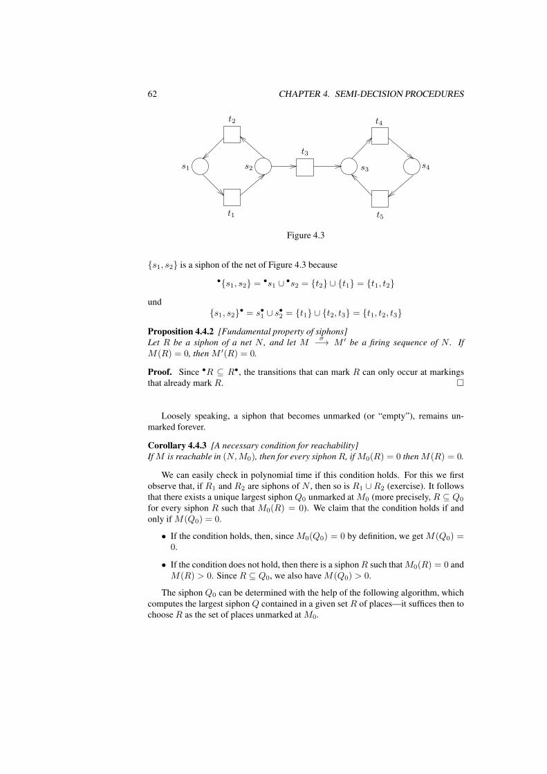
62 CHAPTER 4. SEMI-DECISION PROCEDURES
t3
s3
t5t1
t2
s1
t4
s4s2
Figure 4.3
{s1, s2} is a siphon of the net of Figure 4.3 because
•{s1, s2} =•s1 ∪
•s2 = {t2} ∪ {t1} = {t1, t2}
und
{s1, s2}• = s•1 ∪ s•2 = {t1} ∪ {t2, t3} = {t1, t2, t3}
Proposition 4.4.2 [Fundamental property of siphons]
Let R be a siphon of a net N , and let Mσ−→ M ′ be a firing sequence of N . If
M(R) = 0, then M ′(R) = 0.
Proof. Since •R ⊆ R•, the transitions that can mark R can only occur at markings
that already mark R. �
Loosely speaking, a siphon that becomes unmarked (or “empty”), remains un-
marked forever.
Corollary 4.4.3 [A necessary condition for reachability]
If M is reachable in (N,M0), then for every siphon R, if M0(R) = 0 then M(R) = 0.
We can easily check in polynomial time if this condition holds. For this we first
observe that, if R1 and R2 are siphons of N , then so is R1 ∪ R2 (exercise). It follows
that there exists a unique largest siphon Q0 unmarked at M0 (more precisely, R ⊆ Q0
for every siphon R such that M0(R) = 0). We claim that the condition holds if and
only if M(Q0) = 0.
• If the condition holds, then, since M0(Q0) = 0 by definition, we get M(Q0) =0.
• If the condition does not hold, then there is a siphon R such that M0(R) = 0 and
M(R) > 0. Since R ⊆ Q0, we also have M(Q0) > 0.
The siphon Q0 can be determined with the help of the following algorithm, which
computes the largest siphon Q contained in a given set R of places—it suffices then to
choose R as the set of places unmarked at M0.

4.4. SIPHONS AND TRAPS 63
Input: A net N = (S, T, F ) and R ⊆ S.
Output: The largest siphon Q ⊆ R.
Initialization: Q := R.
begin
while there are s ∈ Q and t ∈ •s such that t /∈ Q• do
Q : = Q \ {s}endwhile
end
Exercise: Show that the algorithm is correct. That is, prove that the algorithm
terminates, and that after termination Q is the largest siphon contained in R.
Proposition 4.4.4 [A necessary condition for liveness]
If (N,M0) is live, then M0 marks every proper siphon of N .
Proof. Let R be a proper siphon of N and let s ∈ R. Since we assume that N is
connected, •s ∪ s• 6= ∅, and, since R is a siphon, s• 6= ∅. Let t ∈ s• 6= ∅. By liveness
some reachable marking enables t, and so some reachable marking marks s, and there-
fore also the siphon R. By Proposition 4.4.3 the initial marking M0 also marks R. �
Again, the condition can be checked with the help of the algorithm above: the con-
dition holds if and only if Q0 = ∅. We now look at deadlock-freedom. We can obtain
a sufficient condition for it, but not one that is easy to check.
Proposition 4.4.5 If M is a dead marking of N , then the set of places unmarked at Mis a siphon of N .
Proof. Let R = {s | M(s) = 0}. For every transition t there is a place s ∈ •t such
that M(s) = 0 (otherwise t would be enabled). So R• contains all transitions of N ,
and therefore •R ⊆ R•. �
Corollary 4.4.6 [A sufficient condition for deadlock-freedom] Let (N,M0) be a Petri
net. If every reachable marking marks all siphons of N , then (N,M0) is deadlock-free.
4.4.2 Traps
Definition 4.4.7 (Trap)
Let N = (S, T, F ) be a trap. A set R ⊆ S of places is a trap if R• ⊆ •R. A trap R is
proper if R 6= ∅.
{s3, s4} is a trap of the net of Figure 4.3.
Proposition 4.4.8 [Fundamental property of traps]
Let R be a trap of a net N and let Mσ−→M ′ be a firing sequence of N . If M(R) > 0,
then M ′(R) > 0.
64 CHAPTER 4. SEMI-DECISION PROCEDURES
Proof. Since •R ⊆ •R, transitions that take tokens from R put tokens in R. �
So, loosely speaking, marked traps stay marked. Notice, however, that this does
not mean that the number of tokens of a trap cannot decrease. The number can go up
or down, just not become 0.
Corollary 4.4.9 [A necessary condition for reachability]
If M is reachable in (N,M0), then for every trap R, if M0(R) > 0 then M(R) > 0.
As in the case of siphons, we can check in polynomial time if this condition holds.
If R1 and R2 are traps of N , then so is R1 ∪ R2 (exercise). So there exists a unique
largest trap Q0 marked at M0 (more precisely, R ⊆ Q0 for every trap R such that
M(R) > 0). It is easy to see that the condition holds if and only if M0(Q0) > 0(exercise).
To compute the largest trap unmarked at M , we can transform the algorithm that
computes the largest siphon contained in a given set of places into an algorithm for
computing the largest trap (exercise).
Recall that checking the sufficient condition for deadlock-freedom was computa-
tionally expensive, because of the form “for every reachable marking ...”. Combining
siphons and traps we obtain an easier-to-check condition.
Proposition 4.4.10 [A sufficient condition for deadlock-freedom]
Let (N,M0) be a Petri net. If every proper siphon of N contains a trap marked at M0,
then (N,M0) is deadlock-free.
Proof. Easy consequence of Corollary 4.4.6 and Proposition 4.4.8. �
The siphon-trap condition cannot be checked in polynomial time unless P=NP
(whether every proper siphon contains a marked trap is an NP-complete problem), but
can be checked with the help of a SAT-solver (see “New algorithms for deciding the
siphon-trap property” by O. Oanea, H. Wimmel, and K. Wolf).
We finally show how to combine S-invariants and traps to prove that Peterson’s
algorithm satisfies the mutual exclusion property. For the Petri net model of Figure 2.8
mutual exclusion means that no reachable marking M satisfies M(p4) ≥ 1∧M(q4) ≥1. We first compute three S-invariants:
(1) M(hold = 1) +M(hold = 2) = 1
(2) M(p2) +M(p3) +M(p4) +M(m1 = f) = 1
(3) M(q2) +M(q3) +M(q4) +M(m1 = f) = 1
and two constraints derived from traps:
(4) M(m1 = f) +M(p2) +M(hold = 1) +M(q3) > 0
(5) M(m2 = f) +M(q2) +M(hold = 2) +M(p3) > 0

4.4. SIPHONS AND TRAPS 65
Assume now M(p4) ≥ 1 ∧M(q4) ≥ 1 holds. We have:
M(p4) ≥ 1 ∧M(q4) ≥ 1
⇒ {(2), (3)}
M(p2) +M(p3) +M(m1 = f) = 0 ∧ M(q2) +M(q3) +M(m2 = f) = 0
⇒ {(1)}
M(m1 = f) +M(p2)+ M(m2 = f) +M(q2)+M(hold = 1) +M(q3) = 0 ∨ M(hold = 2) +M(p3) = 0
Contradicts (4) Contradicts (5)

66 CHAPTER 4. SEMI-DECISION PROCEDURES

Chapter 5
Petri net classes with efficient
decision procedures
In the three sections of this chapter we study three classes of Petri nets: S-systems,
T-systems, and free-choice systems. The sections have a similar structure. After the
definition of the class, we introduce three theorems: the Liveness, Boundedness, and
Reachability Theorem. The Liveness Theorem characterizes the live Petri nets in the
class. The Boundedness Theorem characterizes the live and bounded systems. The
Reachability Theorem characterizes the reachable markings of the live and bounded
systems. The proof of the theorems requires some results about the structure of S- and
T-invariants of the class, which we also present.
The theorems immediately yield decision procedures for Liveness, Boundedness
and Reachability whose complexity is much lower than those for general Petri nets.
At the end of the section we present a final theorem, the Shortest Path Theorem,
which gives an upper bound for the length of the shortest firing sequence leading to a
given reachable marking.
The reader may ask why boundedness only for live Petri nets, and why reachability
only for live and bounded Petri nets. A first reason is that, in many application areas,
a Petri net model of a correct system must typically be live and bounded, and so,
when one of these properties fails, it does not make much sense to further analyze
the model. The second reason is that, interestingly, the general characterization of the
bounded systems or the reachable markings is more complicated and less elegant than
the corresponding characterization for live or live and bounded Petri nets.
The proofs of the theorems are very easy for S-systems, a bit more involved for T-
systems, and relatively complex for free-choice systems. For this reason we just sketch
the proofs for S-systems, explain the proofs in some detail for T-systems, and omit
them for free-choice systems.
67

68CHAPTER 5. PETRI NET CLASSES WITH EFFICIENT DECISION PROCEDURES
5.1 S-Systems
Definition 5.1.1 (S-nets, S-systems) A net N = (S, T, F ) is a S-net if |•t| = 1 = |t•|for every transition t ∈ T . A Petri net (N,M0) is a S-system if N if N is a S-net.
Proposition 5.1.2 (Fundamental property of S-systems)
Let (N,M0) be a S-system with N = (S, T, F ). Then M0(S) = M(S) for every
reachable marking M .
Proof. Every transition consumes one token and produces one token. �
Theorem 5.1.3 [Liveness Theorem] A S-system (N,M0) where N = (S, T, F ) is live
iff N is strongly connected and M0(S) > 0.
Proof. (Sketch.)
(⇒): If N is not strongly connected, then there is an arc (s, t) such that N has no path
from t to s. For every marked place s′ such that there is a path from s′ to s, we fire the
transitions of the path to bring the tokens in s′ to s, and then fire t to empty s. We have
then reached a marking from which no tokens can “travel” back to s, and so a marking
from which t cannot occur again. So (N,M0) is not live.
If M0 marks no places, then no transition can occur, and (N,M0) is not live.
(⇐): If N is strongly connected and M0 puts at least one token somewhere, then
the token can freely move, reach any other place, and so enable any transition again. �
Theorem 5.1.4 [Boundedness Theorem] A live S-system (N,M0) where N = (S, T, F )is b-bounded iff M0(S) ≤ b.
Proof. Trivial. �
Exercise: give a counterexample for non-live S-systems.
Theorem 5.1.5 [Reachability Theorem] Let (N,M0) be a live S-system and let M be
a marking of N . M is reachable from M0 iff M0(S) = M(S).
Proof. N is strongly connected by Proposition 5.1.3. So we are free to distribute the to-
kens of M0 in an arbitrary way, and reach any marking M , as long as M(S) = M0(S).�
Proposition 5.1.6 [S-invariants of S-nets] Let N = (S, T, F ) be a connected S-net. A
vector I : S → Q is a S-invariant of N iff I = (x, . . . , x) for some x ∈ Q.

5.2. T-SYSTEMS 69
Proof.
Each transition t ∈ T has exactly one input place st and an output place s′t. So we
have∑
s∈•t
I(s) = I(st) and∑
s∈t•
I(s) = I(s′t)
and therefore
I is a S-invariant
⇔ {Proposition 4.3.5 (alternative definition of S-invariant)}∀t ∈ T : I(st) = I(s′t)
⇔ {N is connected}∀s1, s2 ∈ S : I(s1) = I(s2)
⇔ { }∃x ∈ Q∀s ∈ S : I(s) = x.
�
5.2 T-systems
Definition 5.2.1 (T-nets, T-systems) A net N = (S;T, F ) is a T-net if |•s| = 1 = |s•|for every place s ∈ S. A system (N,M0) is a T-system if N is a T-net.
Notation: Let γ be a circuit of a net N and let M be a marking of N . We denote by
M(γ) the number if tokens of γ under M , that is, M(γ) =∑
s∈γ M(s).
Proposition 5.2.2 (Fundamental property of T-systems) Let γ be a circuit of a T-
systems (N,M0) and let M be a reachable marking. Then M(γ) = M0(γ).
Proof. Firing a transition does not change the number of tokens of γ. If the transition
does not belong to the circuit, then the distribution of tokens in the circuit does not
change. If the transition belongs to the circuit, then it removes one token from a place
of the circuit, and adds a token to another place. The token count does not change. �
5.2.1 Liveness
Theorem 5.2.3 [Liveness Theorem] A T-system (N,M0) is live iff M0(γ) > 0 for
every circuit γ of N .
Proof.
(⇒) Let γ be a circuit with M0(γ) = 0. By Proposition 5.2.2 we have M(γ) = 0for every reachable marking M . So no transition of γ can ever occur.
(⇐) Let t be an arbitrary transition and let M be a reachable marking. We show
that some marking reachable from M enables t. Let SM be the set of places s of N

70CHAPTER 5. PETRI NET CLASSES WITH EFFICIENT DECISION PROCEDURES
satisfying the following property: there is a path from s to t that contains no place
marked at M . We proceed by induction on |SM |. Basis: |SM | = 0. Then M(s) > 0for every place s ∈ • t, and so M enables t.Step: |SM | > 0. By the fundamental property of T-systems, every circuit of N is
marked at M . So there is a path Π such that:
(1) Π leads to t;
(2) M marks no place of Π;
(3) Π has maximal length (that is, no path longer than Π satisfies (1) and (2)).
Let u be the first element of Π. By (3) u is a transition and M marks all places of•u. So M enables u. Moreover, we have u 6= t because M does not enable t. Let
Mu−→M ′. We show that SM ′ ⊂ SM , and so that |SM ′ | < |SM |.
1. SM ′ ⊆ SM
Let s ∈ SM ′ . We show s ∈ SM . There is a path Π′ = s . . . t containing no place
marked at M ′. Assume Π′ contains a place r marked at M . Since M ′(r) = 0
and Mu−→ M ′ we have u ∈ r• and so {u} = r•. So u is the successor of r in
Π′. Since u 6= t, M ′ marks the successor of u in Π′, contradicting the definition
of Π′.
2. SM ′ 6= SM . Let s be the successor of u in Π. Then s ∈ SM but s 6∈ SM ′ ,
because M ′(s) > 0.
By induction hypothesis there is a firing sequence M ′ σ−→ M ′′ such that M ′′ enables
t. It follows Mu−→ M ′ σ
−→ M ′′, and so M ′′ is a marking reachable from M that
enables t. �
5.2.2 Boundedness
Theorem 5.2.4 [Boundedness Theorem] A place s of a live T-system (N,M0) is b-bounded iff it belongs to some circuit γ such that M0(γ) ≤ b.
Proof. (⇐) Follows from the fundamental property of T-systems (Proposition 5.2.2).
(⇒) Let M be a reachable marking such that M(s) is maximal. We have M(s) ≤ b.Define the marking L as follows:
L(r) =
{
M(r) if r 6= s0 if r = s
We claim that (N,L) is not live. Otherwise there would be a firing sequence Lσ−→ L′
such that L′(s) > 0, and by the Monotonicity Lemma we would have Mσ−→ M ′ for
some marking M ′ satisfying M ′(s) = L′(s)+M(s) > M(s), contradicting the maxi-
mality of M(s). By the Liveness Theorem some circuit γ is unmarked at L but marked

5.2. T-SYSTEMS 71
at M . Since L and M only differ in the place s, the circuit γ contains s. Further, sis the only place of γ marked at M . So M(γ) = M(s), and since M(s) ≤ b we get
M(γ) ≤ b. �
Corollary 5.2.5 Let (N,M0) be a live T-system
1. A place of N is bounded iff it belongs to some circuit.
2. Let s be a bounded place. Then
max{M(s) |M0∗−→M} = min{M0(γ) | γ contains s}
3. (N,M0) is bounded iff N is strongly connected.
Proof. Exercise �
5.2.3 Reachability
We need to have a closer look at the T-invariants of T-systems.
Proposition 5.2.6 [T-invariants of T-nets] Let N = (S, T, F ) be a connected T-net. A
vector J : T → Q is a T-invariant iff J = (x . . . x) for some x ∈ Q.
Proof. Dual of the proof of Proposition 5.1.6. �
Theorem 5.2.7 [Reachability Theorem] Let (N,M0) be a live T-system. A marking
M is reachable from M0 iff M0 ∼M .
Proof. (⇒) Proposition 4.3.11
(⇐) By Theorem 4.3.12 there is a rational vector X such that
M = M0 +N.X (5.1)
The vector J = (1, 1, . . . , 1) is a T-invariant of N (Proposition 5.2.6). So we have
N · (X + λJ) = N ·X
for every λ ∈ Q. So without loss of generality we can assume X ≥ 0.
Let T be the set of transitions of N . We show:
(1) There is a vector Y : T → IN such that M = M0 +N · Y . Let Y be the vector
with Y (t) = ⌈X(t)⌉ for every transition t (⌈x⌉ denotes the smallest integer
larger than or equal to x). By (5.1) we have
M(s) = M0(s) +X(t1)−X(t2)
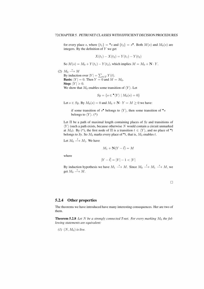
72CHAPTER 5. PETRI NET CLASSES WITH EFFICIENT DECISION PROCEDURES
for every place s, where {t1} = •s and {t2} = s•. Both M(s) and M0(s) are
integers. By the definition of Y we get
X(t1)−X(t2) = Y (t1)− Y (t2)
So M(s) = M0 + Y (t1)− Y (t2), which implies M = M0 +N · Y .
(2) M0∗−→M
By induction over |Y | =∑
t∈T Y (t).Basis: |Y | = 0. Then Y = 0 and M = M0.
Step: |Y | > 0.
We show that M0 enables some transition of 〈Y 〉. Let
Sy = {s ∈ •〈Y 〉 |M0(s) = 0}
Let s ∈ Sy . By M0(s) = 0 and M0 +N · Y = M ≥ 0 we have:
if some transition of s• belongs to 〈Y 〉, then some transition of •sbelongs to 〈Y 〉. (*)
Let Π be a path of maximal length containing places of Sy and transitions of
〈Y 〉 (such a path exists, because otherwise N would contain a circuit unmarked
at M0). By (*), the first node of Π is a transition t ∈ 〈Y 〉, and no place of •tbelongs to Sy. So M0 marks every place of •t, that is, M0 enables t.
Let M0t−→M1. We have
M1 +N(Y − ~t) = M
where
|Y − ~t| = |Y | − 1 < |Y |
By induction hypothesis we have M1∗−→ M . Since M0
t−→ M1
∗−→ M , we
get M0∗−→M .
�
5.2.4 Other properties
The theorems we have introduced have many interesting consequences. Her are two of
them.
Theorem 5.2.8 Let N be a strongly connected T-net. For every marking M0 the fol-
lowing statements are equivalent:
(1) (N,M0) is live.
5.2. T-SYSTEMS 73
(2) (N,M0) is deadlock-free.
(3) (N,M0) has an infinite firing sequence.
Proof. (1)⇒ (2)⇒ (3) follow immediately from the definitions. We show (3)⇒ (1).
Let M0σ−→ be an infinite firing sequence. We claim that every transition of N
occurs in σ. Since N is strongly connected, (N,M0) is bounded (Theorem 5.2.4). Let
σ = t1 t2 t3 . . ., and M0t1−→ M1
t2−→ M2t3−→ . . .. Since (N,M0) is bounded,
there are indices i and j with i < j such that Mi = Mj . Let σij be the subsequence
of σ containing the transitions between Mi and Mj . By the fundamental property of
T-invariants (Proposition 4.3.15) ~σij is a T-Invariant . By Proposition 5.2.6 there is
n ∈ N such that ~σij = (n . . . n). So every transition of N occurs in σij , and so the
same holds for σ.
Since every transition of N occurs in σ, for every place and every circuit of Nsome marking reached during the execution of N marks the place or the circuit. By
the fundamental property of T-systems, all circuits of N are marked at M0. By the
Liveness Theorem (Theorem 5.2.3), (N,M0) is live. �
Theorem 5.2.9 [Genrich’s Theorem] Let N be a strongly connected T-net with at least
one place and one transition. There is a marking M0 such that (N,M0) is live and 1-
bounded.
Proof. Since N is strongly connected, any marking that puts tokens on all places of
N is live, because it marks all circuits (Liveness Theorem), and bounded, because all
markings of N are (Corollary 5.2.5).
Let (N,M) be live and bounded, but not 1-bounded. We construct another live
marking L of N satisfying the following two conditions:
(1) L(γ) ≤M(γ) for every circuit γ of N , and
(2) L(γ) < M(γ) for at least one circuit γ.
By Theorem 5.2.4, at least one place of N has a smaller bound under L as under M .
Iterating this construction we obtain a 1-bounded marking of N .
Let s be a non-1-bounded place of (N,M). Some reachable marking M ′ satisfies
M ′(s) ≥ 2. Let L be the marking that puts exactly one token in s, and as many tokens
as M elsewhere.
Since M is live, it marks all circuits of N . By constructionL also marks all circuits,
and so L is also live. Condition (1) is a consequence of the definition of L. Condition
(2) holds for all circuits containing s (and there is at least one, because N is strongly
connected). �

74CHAPTER 5. PETRI NET CLASSES WITH EFFICIENT DECISION PROCEDURES
free-choice not free-choice
Figure 5.1
5.3 Free-Choice Systems
Definition 5.3.1 (Free-Choice nets, Free-Choice systems) A net N = (S, T, F ) is
free-choice if s• × •t ⊆ F for every s ∈ S and t ∈ T such that (s, t) ∈ F . A Petri net
(N,M0) is free-choice if N is a free-choice net..
This definition is very concise and moreover symmetric with respect to places and
transitions. If the reader finds it cryptic, the following equivalent definitions may help.
Proposition 5.3.2 [Alternative definitions of free-choice nets]
(1) A net is free-choice if for every two transitions t1, t2:
(t1 6= t2 ∧•t1 ∩
•t2 6= ∅)⇒•t1 = •t2
(2) A net is free-choice if for every two places s1, s2:
(s1 6= s2 ∧ s•1 ∩ s•2 6= ∅)⇒ s•1 = s•2
Proof. Exercise. �
Figure 5.1 illustrates these definitions.
Clearly, S- and T-systems are special cases of free-choice systems (see Figure 5.2).
5.3.1 Liveness
We showed in the last chapter that a Petri net in which every siphon contains an initially
marked trap is deadlock-free, but the converse does not hold. For free-choice systems
we obtain Commoner’s Theorem, a much stronger result characterizing liveness.
Theorem 5.3.3 [Commoner’s Liveness Theorem] A free-choice system (N,M0) is live
iff every siphon of N contains a trap marked at M0.
Proof. We sketch the following direction: if every siphon of N contains a trap
marked at M0, then (N,M0) is live. We need the following definitions. Let M be a
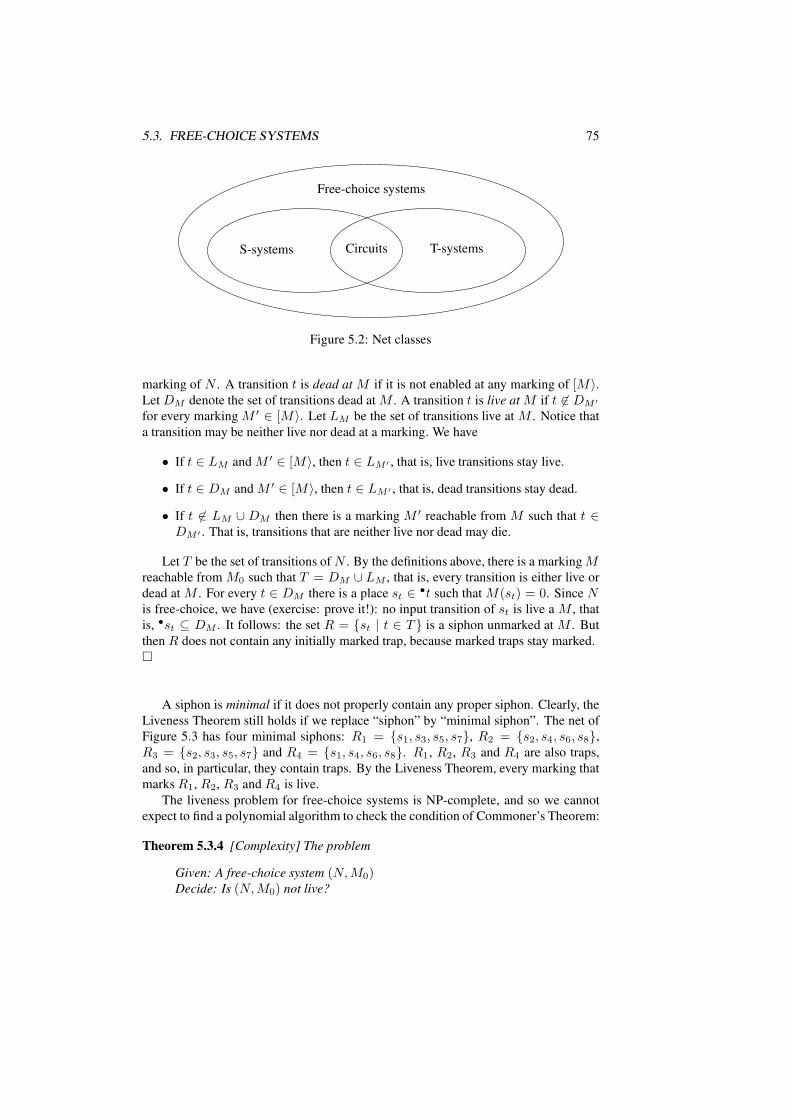
5.3. FREE-CHOICE SYSTEMS 75
Circuits T-systemsS-systems
Free-choice systems
Figure 5.2: Net classes
marking of N . A transition t is dead at M if it is not enabled at any marking of [M〉.Let DM denote the set of transitions dead at M . A transition t is live at M if t 6∈ DM ′
for every marking M ′ ∈ [M〉. Let LM be the set of transitions live at M . Notice that
a transition may be neither live nor dead at a marking. We have
• If t ∈ LM and M ′ ∈ [M〉, then t ∈ LM ′ , that is, live transitions stay live.
• If t ∈ DM and M ′ ∈ [M〉, then t ∈ LM ′ , that is, dead transitions stay dead.
• If t 6∈ LM ∪ DM then there is a marking M ′ reachable from M such that t ∈DM ′ . That is, transitions that are neither live nor dead may die.
Let T be the set of transitions of N . By the definitions above, there is a marking Mreachable from M0 such that T = DM ∪ LM , that is, every transition is either live or
dead at M . For every t ∈ DM there is a place st ∈ •t such that M(st) = 0. Since Nis free-choice, we have (exercise: prove it!): no input transition of st is live a M , that
is, •st ⊆ DM . It follows: the set R = {st | t ∈ T } is a siphon unmarked at M . But
then R does not contain any initially marked trap, because marked traps stay marked.
�
A siphon is minimal if it does not properly contain any proper siphon. Clearly, the
Liveness Theorem still holds if we replace “siphon” by “minimal siphon”. The net of
Figure 5.3 has four minimal siphons: R1 = {s1, s3, s5, s7}, R2 = {s2, s4, s6, s8},R3 = {s2, s3, s5, s7} and R4 = {s1, s4, s6, s8}. R1, R2, R3 and R4 are also traps,
and so, in particular, they contain traps. By the Liveness Theorem, every marking that
marks R1, R2, R3 and R4 is live.
The liveness problem for free-choice systems is NP-complete, and so we cannot
expect to find a polynomial algorithm to check the condition of Commoner’s Theorem:
Theorem 5.3.4 [Complexity] The problem
Given: A free-choice system (N,M0)Decide: Is (N,M0) not live?
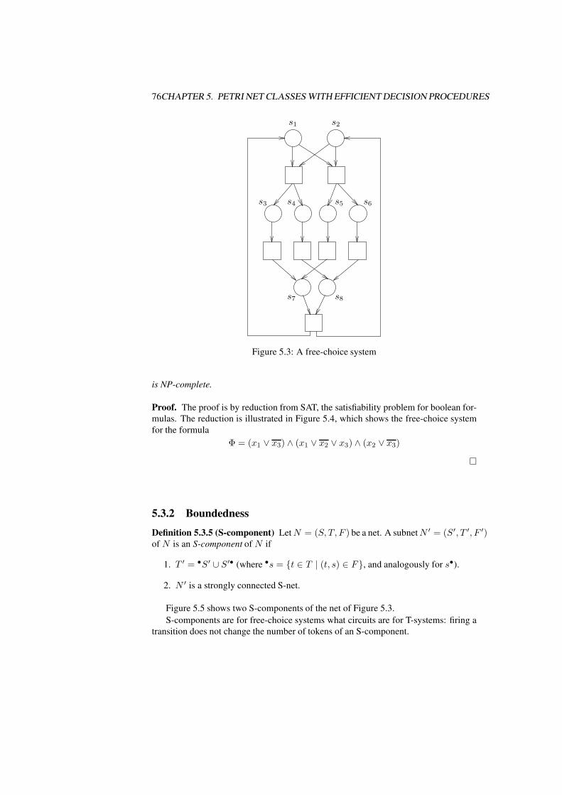
76CHAPTER 5. PETRI NET CLASSES WITH EFFICIENT DECISION PROCEDURES
s1 s2
s3 s4 s5 s6
s7 s8
Figure 5.3: A free-choice system
is NP-complete.
Proof. The proof is by reduction from SAT, the satisfiability problem for boolean for-
mulas. The reduction is illustrated in Figure 5.4, which shows the free-choice system
for the formula
Φ = (x1 ∨ x3) ∧ (x1 ∨ x2 ∨ x3) ∧ (x2 ∨ x3)
�
5.3.2 Boundedness
Definition 5.3.5 (S-component) LetN = (S, T, F ) be a net. A subnetN ′ = (S′, T ′, F ′)of N is an S-component of N if
1. T ′ = •S′ ∪ S′• (where •s = {t ∈ T | (t, s) ∈ F}, and analogously for s•).
2. N ′ is a strongly connected S-net.
Figure 5.5 shows two S-components of the net of Figure 5.3.
S-components are for free-choice systems what circuits are for T-systems: firing a
transition does not change the number of tokens of an S-component.

5.3. FREE-CHOICE SYSTEMS 77
x1x1
A1 A2 A3
x2 x3x2 x3
C1 C2 C3
False
Figure 5.4: Free-choice system for the formula Φ

78CHAPTER 5. PETRI NET CLASSES WITH EFFICIENT DECISION PROCEDURES
s1
s3 s5
s7
s2
s4 s6
s8
Figure 5.5: S-components of the net of Figure 5.3
Proposition 5.3.6 Let (N,M0) be a Petri net and let N ′ = (S′, T ′, F ′) be an S-
component of N . Then M0(S′) = M(S′) for every marking M reachable from M0.
Proof. Firing a transition either takes no tokens from a place of the component and
adds none, or it takes exactly one token and adds exactly one token. �
Theorem 5.3.7 [Hack’s Boundedness Theorem] Let (N,M0) be a live free-choice sys-
tem. (N,M0) is bounded iff every place of N belongs to a S-component.
Proof. (⇐) Exercise
(⇒) (Sketch). We first show that every minimal siphon N is the set of places of a
S-component. Then we show that every place is contained in some minimal siphon. �
Proposition 5.3.8 [Place bounds] Let (N,M0) be a live and bounded free-choice sys-
tem and let s be a place of N . We have
max{M(s) |M0∗−→M} =
min{M0(S′) | S′ is the set of places of a S-component of N}

5.3. FREE-CHOICE SYSTEMS 79
Figure 5.6: Clusters of the net of Figure 5.3
Proof. Analogous to the Boundedness Theorem for T-systems. �
Theorem 5.3.4 shows that there is no polynomial algorithm for Liveness (unless
P = NP ). Now we ask ourselves what is the complexity of deciding if a free-choice
system is simultaneously live and bounded. We can of course first use the decision
procedure for liveness, and then, if the net is live, check the condition of the Bounded-
ness Theorem. But there are more efficient algorithms.1. The fastest known algorithm
runs in O(n ·m) time for a net with n places and m transitions. A not so efficient but
simpler algorithm follows immediately from the next theorem:
Definition 5.3.9 (Cluster) Let N = (S, T, F ) be a net. A cluster is an equivalence
class of the equivalence relation ((F ∩ (S × T )) ∪ (F ∩ (S × T ))−1)∗.
Figure 5.6 shows the clusters of the net of Figure 5.3.
1Compare with this: in order to decide if a number is divisible by 100.000, we can first check if it is
divisible by 3125, and, if so, if it is divisible by 32. However, there is a faster procedure: check if the last
five digits are zeros.

80CHAPTER 5. PETRI NET CLASSES WITH EFFICIENT DECISION PROCEDURES
Theorem 5.3.10 [The Rank Theorem] A free-choice system (N,M0) is live and bounded
iff
1. N has a positive S-invariant.
2. N has a positive T-invariant.
3. The rank of the incidence matrix (N) is equal to c− 1, where c is the number of
clusters of N .
4. Every siphon of N is marked under M0.
Proof. Omitted. �
Conditions (1) and (2) can be checked using linear programming, condition (3)
using well-known algorithms of linear algebra, and condition (4) with the algorithm of
Section 4.4.1.
5.3.3 Reachability
Theorem 5.3.11 Reachability is NP-complete for live and bounded free-choice nets.
Proof. Exercise: find a reduction from SAT. �
However, for systems satisfying an additional condition there is a polynomial algo-
rithm. A Petri net (N,M0) is cyclic if, loosely speaking, it is always possible to return
to the initial marking. Formally: ∀M ∈ [M0〉 : M0 ∈ [M〉. We have:
Theorem 5.3.12 [Reachability Theorem] Let (N,M0) be a live, bounded, and cyclic
free-choice system. A marking M of N is reachable from M0 iff M0 ∼M .
Proof. Omitted. �
Corollary 5.3.13 The problem
Given: a live, bounded, and cyclic free-choice system (N,M0) and a
marking MDecide: Is M reachable?
can be solved in polynomial time.
This result is only useful if we are able to check efficiently if a live and bounded
free-choice system is cyclic. The following theorem shows that this is the case:
Theorem 5.3.14 A live and bounded free-choice system (N,M0) is cyclic iff M0 marks
every proper trap of N .
Proof. Omitted. �