PETRA Quick Start Manual
139
1996-2006 IHS All rights reserved PETRA ® © PETRA from IHS ® Quick Start Manual
-
Upload
juan-carlos-romero-gelvez -
Category
Documents
-
view
22 -
download
5
Transcript of PETRA Quick Start Manual

1996-2006 IHSAll rights reserved
PETRA
®
©
PETRA
from IHS
®
Quick StartManual


PETRA Quick Start Manual®
1996-2006 8801 South Yale, Suite 380 Tulsa, OK 74137-3548
Phone 918.971.7071 www.ihs.com
©
••
IHS
IHS

Copyright
©1996-2006 IHS. All rights reserved. This manual, as well as the software described in it, is furnished under license and may only beused or copied in accordance with the terms of such license. The information in this manual is furnished for informational use only, issubject to change without notice, and should not be construed as a commitment by IHS. IHS assumes no responsibility for theconsequences of any errors or inaccuracies that may appear in this book.
While every precaution has been taken in the preparation of this document, the publisher and the author assume no responsibility for errors or omissions, or for damages resulting from the use of information contained in this document or from the use of programs and source code that may accompany it. In no event shall the publisher and the author be liable for any loss of profit or any other commercial damage caused or alleged to have been caused directly or indirectly by this document.
Except as permitted by the license for this manual, no part of this publication may be reproduced, stored in a retrieval system, ortransmitted, in any form or by any means, electronic, mechanical, recording, or otherwise, without the prior written permission of IHS.
Trademarks
PETRA® is a trademark of IHS.
Windows® 2000/XP/Vista are registered trademarks of Microsoft Corporation.
Companies, names, and dates used in examples herein are fictitious unless otherwise noted.
Government Restricted RightsFor units of the Department of Defense, use, duplication, or disclosure by the Government is subject to restrictions as set forth insubparagraph (c)(1)(ii) of the Rights in Technical Data and Computer Software clause at DFARS 252.227-7013.Contractor/manufacturer is IHS, 8801 South Yale, Suite 380, Tulsa, OK 74137-3548.
If the Commercial Computer Software Restricted Rights clause at FAR 52.227-19 or its successors apply, the Software andDocumentation constitute restricted computer software as defined in that clause and the Government shall not have the license forpublished software set forth in subparagraph (c)(3) of that clause.
Printed: March 2007 in Tulsa, Oklahoma
Getting Started

Table of Contents
................................................................................................1Part I Introduction
................................................................................................................................... 11 Tutorial and Sample Projects
................................................................................................................................... 12 Hardware Requirements
................................................................................................................................... 23 Software Installation
................................................................................................................................... 24 PETRA DEMO
................................................................................................4Part II PETRA Tutorial Overview
................................................................................................................................... 41 Function Keys
................................................................................................................................... 82 PETRA Modules and Tools
................................................................................................................................... 83 Main Module
................................................................................................................................... 104 Mapping Tool
................................................................................................................................... 105 Cross-Section Tool
................................................................................................................................... 116 Spread Sheet Tool
................................................................................................................................... 117 Log Cross Plot Tool
................................................................................................................................... 118 Z Cross Plot Tool
................................................................................................................................... 119 2D Seismic Tool
................................................................................................................................... 1110 Log Histogram Tool
................................................................................................................................... 1211 Production Analysis Tool
................................................................................................................................... 1212 PetraSeis Tool
................................................................................................................................... 1213 Thematic Mapper
................................................................................................................................... 1314 3d Visualizer
................................................................................................................................... 1315 Slip Logs Module
................................................................................................................................... 1316 Calculations and Transformation Tools
................................................................................................................................... 1417 Units
................................................................................................................................... 1418 Help
................................................................................................................................... 1419 Last
................................................................................................15Part III Data Organization and Concepts
................................................................................................................................... 151 PETRA Projects
................................................................................................................................... 152 Sharing Projects
.......................................................................................................................................................... 15Creating a Shared Project
.......................................................................................................................................................... 18Shared Project Data is Live ................................................................................................................................... 193 Project Data
.......................................................................................................................................................... 19Unique Well Identifier (UWI)
.......................................................................................................................................................... 19Well Sequence Number (WSN)
.......................................................................................................................................................... 19Well Label
.......................................................................................................................................................... 19Zones
IContents
I
© 2007 ... IHS

.......................................................................................................................................................... 20Zone Data Items
.......................................................................................................................................................... 20Well Selection
.......................................................................................................................................................... 21Missing or "Null" Data Values ................................................................................................................................... 214 Creating a New Project
.......................................................................................................................................................... 23Importing Well Data
.......................................................................................................................................................... 24Importing Tabular ASCII Well Data
.......................................................................................................................................................... 25Importing Digital Log Data ................................................................................................................................... 285 Project Menus
.......................................................................................................................................................... 28Project>Remarks File Menu
.......................................................................................................................................................... 29Project>Import Menu
.......................................................................................................................................................... 30Project>Export Menu
.......................................................................................................................................................... 31Project>Close Menu
.......................................................................................................................................................... 31Project>Reopen Menu
.......................................................................................................................................................... 32Project>Settings Menu ......................................................................................................................................................... 32Program Options............................................................................................................................................................ 32Set Map Projection............................................................................................................................................................ 32System Colors............................................................................................................................................................ 32Well Symbols............................................................................................................................................................ 33Reset Module............................................................................................................................................................ 33Reset Default UWI Column Widths......................................................................................................................................................... 33Project>Exit Menu......................................................................................................................................................... 34Project>Prospect Menu......................................................................................................................................................... 34Help
................................................................................................35Part IV Main Module
................................................................................................................................... 351 Switching Between Modules
................................................................................................................................... 352 Opening the "Tutorial" Project
................................................................................................................................... 383 Main Module Overview
.......................................................................................................................................................... 38Projection for Projects ................................................................................................................................... 404 Sorting the Well List
................................................................................................................................... 415 Project Tab
................................................................................................................................... 436 Well Tab
.......................................................................................................................................................... 44Adding a New Well Manually
.......................................................................................................................................................... 46Changing the Unique Well Identifier
.......................................................................................................................................................... 46Deleting a Single Well
.......................................................................................................................................................... 46Deleting Multiple Wells ................................................................................................................................... 477 Location Tab
.......................................................................................................................................................... 47Deviated Wells
.......................................................................................................................................................... 47Displaying the Survey Data
.......................................................................................................................................................... 48Locking Projection
.......................................................................................................................................................... 48Locking Locations ................................................................................................................................... 498 Fm Tops Tab
.......................................................................................................................................................... 50Printing Tops
.......................................................................................................................................................... 50New Top
.......................................................................................................................................................... 50Top Aliases
.......................................................................................................................................................... 51Show Tops By Source
.......................................................................................................................................................... 51Reordering Tops
.......................................................................................................................................................... 51Formation Tops – Maintenance ................................................................................................................................... 529 Zones Tab
.......................................................................................................................................................... 54Creating a New Zone
Getting StartedII
© 2007 ... IHS

.......................................................................................................................................................... 55Adding New Zone Variables or "Items" ................................................................................................................................... 5610 Logs Tab
................................................................................................................................... 5711 IP Tests Tab
................................................................................................................................... 5812 Fm Tests Tab
................................................................................................................................... 5813 Cores Tab
................................................................................................................................... 5814 Perfs/Shows Tab
................................................................................................................................... 5915 Production Tab
.......................................................................................................................................................... 60Computing Cumulative Production Data ................................................................................................................................... 6416 Prod Cums Tab
................................................................................................................................... 6517 Rasters Tab
................................................................................................................................... 6618 Other Tab
.......................................................................................................................................................... 66Casing Details
.......................................................................................................................................................... 66Fault Cuts
.......................................................................................................................................................... 66Pd Sym
.......................................................................................................................................................... 67Well History
.......................................................................................................................................................... 67Liner Details
.......................................................................................................................................................... 67Cement
.......................................................................................................................................................... 68Velocity
................................................................................................69Part V Log Image Calibration
................................................................................................................................... 691 Straightening An Image
................................................................................................................................... 772 Depth Calibration - Log Image
................................................................................................................................... 773 Image Groups
................................................................................................................................... 784 Calibrating A Log Image
................................................................................................................................... 795 The Image Calibration Tool Bar
................................................................................................................................... 826 Assign A Group Name
................................................................................................................................... 827 Define the Calibration Depths
................................................................................................................................... 848 Define the Left and Right Edges of the Image
................................................................................................................................... 849 Define the Log Header Section
................................................................................................................................... 8510 Define the Log Footer Section
................................................................................................................................... 8611 Deleting Calibration Depths
................................................................................................................................... 8612 Saving the Calibration File
................................................................................................................................... 8613 Loading a Calibration File
................................................................................................87Part VI Mapping Module
................................................................................................................................... 871 Mapping Module Overview
................................................................................................................................... 892 Land Grid Overlay
................................................................................................................................... 893 Selecting a Well On the Map
................................................................................................................................... 904 Viewing Data For a Specific Well
................................................................................................................................... 925 Finding A Specific Well
................................................................................................................................... 936 Zooming
................................................................................................................................... 937 Panning and Scrolling
IIIContents
III
© 2007 ... IHS

................................................................................................................................... 938 Posted Base Maps
................................................................................................................................... 939 Selecting and Formatting Posted Data
................................................................................................................................... 9510 Contour Maps
.......................................................................................................................................................... 95Creating a Structure Map Grid
.......................................................................................................................................................... 96Structure Map Contouring
.......................................................................................................................................................... 97Contour Range and Color Palette
.......................................................................................................................................................... 97Contouring With Faults
.......................................................................................................................................................... 97Creating An Isopach ................................................................................................................................... 10111 Bubble Maps
................................................................................................................................... 10212 Map Overlay Utility
.......................................................................................................................................................... 102Using WinTab driver and a Digitizer Tablet
.......................................................................................................................................................... 102Overlay Tool Bar
.......................................................................................................................................................... 104Adding an Overlay Line ......................................................................................................................................................... 104Overlay Line Classes......................................................................................................................................................... 105Editing Line Attributes......................................................................................................................................................... 106Moving Lines and Line Points.......................................................................................................................................................... 106Adding Overlay Text ......................................................................................................................................................... 106Editing Text Attributes......................................................................................................................................................... 106Moving Text
................................................................................................................................... 10713 Capturing Data with a Digitizer
................................................................................................................................... 10714 Using Footage Calls to Spot a Well
................................................................................................................................... 11215 Using the Mouse to Add a New Well
................................................................................................................................... 11316 Using the Mouse to Move a Well Locaton
................................................................................................................................... 11417 Using the Mouse to Update Missing Well
................................................................................................115Part VII Cross Section Module
................................................................................................................................... 1151 Starting A Cross Section
.......................................................................................................................................................... 116Automatic Structure Depth Using Formation Tops
.......................................................................................................................................................... 118Selecting Digital Log Curves
.......................................................................................................................................................... 121Stratrigraphic Cross Section
.......................................................................................................................................................... 121Correlating Formation Tops - Method 1
.......................................................................................................................................................... 123Correlating Formation Tops - Method 2 ................................................................................................................................... 1232 Cross Sections with Raster Images
.......................................................................................................................................................... 123Cross Section - Log Image Display Options ......................................................................................................................................................... 123Available Image Groups......................................................................................................................................................... 123Image Groups To Display......................................................................................................................................................... 124Group Options Tab......................................................................................................................................................... 124General Tab......................................................................................................................................................... 126Memory Tab......................................................................................................................................................... 126File Tab......................................................................................................................................................... 126Misc Tab.......................................................................................................................................................... 126Cross Sectiuon - Log Image Calibration Net Pay ......................................................................................................................................................... 126Pay Tool Bar
Getting StartedIV
© 2007 ... IHS

Introduction 1
© 2007 ... IHS
1 Introduction
Introduction to PETRA®
Congratulations and thank you for selecting PETRA, the latest advance in PC software for thepetroleum industry. PETRA impacts today's prospect generation and acquisition studies withtomorrow's technology. Its features are designed to enhance the decision-making process andstrengthen your competitiveness. PETRA couples a powerful well database with easy-to-usemapping, cross section, and log analysis tools.
PETRA is designed for the Windows 2000/XP/Vista environment, and is focused on improvingthe productivity of asset teams composed of geologists, geophysicists, petrophysicists, andreservoir engineers. PETRA provides a unique solution to data management, manipulation,visualization and integration of geological, geophysical, petrophysical and engineering data. Real-world proven functionality combined with the latest user interface technology allows easytransformation from raw well data to understanding critical reservoir parameters. Results can bequickly visualized using the interactive mapping, cross sections, log plots, cross-plots, and customspreadsheets.
This manual contains a step-by-step tutorial intended to teach the first time user the basic skillsfor using PETRA. By reading this tutorial, you will learn how to navigate the "Main" module toview and edit data, open the "Map" module to create various maps including contour maps, andto open the "Cross Section" module to correlate formation tops from a cross section display.
1.1 Tutorial and Sample Projects
When the Demo version of PETRA is downloaded a project, called "SAMPLE", will be installedalong with the PETRA program files. The "sample" project contains identical data to the"tutorial" project plus additional data and computed results, such as, grid files, and containsspecific default values to speed the viewing process. The "Tutorial" project is loaded when youdownload and install the "Full Evaluation" version of PETRA.
This tutorial utilizes the "TUTORIAL" project database, which is installed along with thePETRA program files. The "TUTORIAL" project contains all data referenced by the tutorialmanual. The "TUTORIAL" project is designed to be used in conjunction with this manual.
We encourage you to read this manual in its entirety. This will help you gain an understanding ofimportant concepts and capabilities that PETRA offers the geo-computing community.
1.2 Hardware Requirements
The minimum hardware required for operation is a personal computer system running theMicrosoft Windows 2000/XP/Vista operating system with a minimum of Pentium classprocessor, 1 GB of RAM and VGA color monitor.
The recommended processor is a Pentium-IV processor or better, 2 GB of RAM, video

Getting Started2
© 2007 ... IHS
resolution of 1024x768 or better, and a color monitor, Dual or Triple monitors are not required,but are supported if the operating system/video card(s) supports them.
Note: No special video cards are required, and PETRA is compatible with a broad range of highperformance video cards, and dual and triple monitor installations.
· The standalone install requires about 110 MB of disk space for program files and the"Tutorial" project.
· The Network install requires about 105 MB of disk space for program files.
· The Network "Client" install requires about 12 MB of disk space for program files andthe "Tutorial" project.
1.3 Software Installation
PETRA is available in both network and standalone versions on a CD-ROM or Internetdownload. When you receive a CD, please follow the specific instructions that are packaged withthe software to insure proper installation.
1.4 PETRA DEMO
The "Demo" version of PETRA has, by design, restricted some of the functionality of theprogram. For example, you cannot create another project, nor can you use the "ProjectàCloseProject" menu. You cannot add new wells, delete existing wells, or delete selected wells.
The "SAMPLE" project, which is provided with the Demo version of PETRA, contains,computed grid files, specific default values, and displays prepared for a quick overview ofPETRA.
When you open the "Demo" version of "PETRA", the "SAMPLE" project will automaticallyopen.
We strongly recommend that you review the tutorial material prior to venturing off on your own.You should at least familiarize yourself with the "Data Organization and Concepts"section.
After looking at the various modules using the "DEMO" version of PETRA and you areinterested in taking a look at the full functionality of the current release of PETRA you can callIHS toll free at 1 (888) PETRA-OK (888-738-7265) or at 1 918-971-7071 x1.
If you have installed the "Full Evaluation Version" of PETRA, you will have a "Welcome toPETRA" dialog screen displayed. There are three choices displayed:
"ReOpen your Last Project""Open an EXISTING Project""Create a NEW Project"

Introduction 3
© 2007 ... IHS
If the "Reopen SAMPLE Project" is displayed, and you have installed the "Full Evaluation"version of PETRA, use the option "Open an Existing Project" and select the "TUTORIAL"project.
To be able to open the "SAMPLE" project in the "Full Evaluation" version of PETRA, close
the "TUTORIAL" project by clicking on the "Close the Current Project" icon , or"ProjectàClose Project" menu.
Click on the "ProjectàBuild Sample Project..." menu.Click on the "ProjectàOpen..." menu.Select "SAMPLE" from the list of projects displayed.
There are three "Icons" in the upper left portion of the "Main" screen. The first icon is "CreateNew Project", the middle icon is "Open An Existing Project" and the third icon is "Close TheCurrent Project".
Suggested topics to preview during your overview:
· Look at the "Formation Tops" tab in the main module and see how easily tops can bemodified.
· View the "Zones" tab to see how PETRA can maintain user-defined variables.· Check the digital log curve-previewing feature located on the "Logs" tab of the main
module.· Look at the monthly production charts by selecting the "Production" tab on the main
module and scrolling through several wells.· Learn how to start the Mapping module from the main tool menu and use the "Optionsà Active/Inactive…" menu to turn on and off some of the predefined displays.
· Learn how to start up the Cross-section module from the Mapping module by using the"Cross Section à Switch To Cross Section Tool".
· Change the digital log curve shading in the Cross section module using the "Logs àDisplay Options" menu.
· Change the tops drawing options in the Cross section module using the "Tops à DisplayOptions" menu.
· Start the Log Cross Plot module from the Main module menu.· Try both XY and ternary cross-plot displays.

Getting Started4
© 2007 ... IHS
2 PETRA Tutorial Overview
This tutorial is designed to familiarize you with data organization, fundamentaldesign concepts and tools that will allow you to manage your geological projectsmore efficiently and make more effective use of your time.
PETRA can reduce the time spent editing and cleaning up data and increase time available fordata analysis and interpretation.
This tutorial will teach you how to:
· Determine which tool to use to accomplish a particular task· Navigate the main module to view and modify well data· Define "zones" for organizing data by geologic interval· How to preview digital well log curves· Create base maps with posted data· Generate structure contour maps· Compute and display isopach contour maps· Compute and display cumulative production using bubble maps· Add and modify overlay lines and text· Create cross section displays using digital logs and/or scanned raster images· Correlate formation tops from a cross section· Create a new project, import well and digital log data.
2.1 Function Keys
There are many function keys and keyboard shortcuts to speed the workflow.
Function Keys – Main
Project>Import>General Well Data From…Generic ASCII File… Ctrl+TProject>IHS Enerdeq>Import Wells From Enerdeq Direct
Connect… Ctrl+Alt+WProject>IHS Enerdeq>Import Production From Enerdeq Direct Connect…Ctrl+Alt+PProject>IHS Enerdeq>View Enerdeq Scout Ticket For Current Well… Ctrl+Alt+SProject>Settings>Program Options… Ctrl+OWells>Select>All Wells Ctrl+AWells>Select>Current Well Only… Ctrl+WWells>Select>Wells By Data Criteria Ctrl+SWells>Go To Well… Ctrl+GWells>Use Previous Well List Ctrl+PUnits>View As Imperial F1Units View As Metric F2Close PETRA Alt+F4Find Text In Well List Ctrl+F

PETRA Tutorial Overview 5
© 2007 ... IHS
FmTops Tab – Right Click popup menu
Lock Item for This Well… Ctrl+LUnlock Item for This Well… Ctrl+ULock Item for Selected Wells… Alt+LUnlock Item for Selected Wells… Alt+U
Zone Tab – Right Click popup menu
Lock Item for This Well… Ctrl+LUnlock Item for This Well… Ctrl+ULock Item for Selected Wells… Alt+LUnlock Item for Selected Wells… Alt+U
Function Keys – Spread Sheet
Wells>Select>All Wells Ctrl+AWells>Select>Wells By Data Criteria Ctrl+SSearch>Find and Replace Ctrl+F
Function Keys – Raster Calibration
Depths>Display Depths As Feet F1Depths>Display Depths As Meters F2Depths>Go To Depth Ctrl+GDigitizing - select segment -Breaking into two segments CtrlDigitizing – select segment -Breaking and Deleting Part of a Segment Ctrl and AltDigitizing – Merge segments - select segment F5Tops>Edit Mode Active Ctrl+T
Function Keys – Raster Log CorrelationImage>Open Image… Ctrl+OImage>Exit Ctrl+XView>Alignment Cursor Ctrl+ADepths>Line Up At Depth… Ctrl+DDepths>Depth Scale… Ctrl+SDepths>Go To First Depth… Ctrl+F
Function Keys – Map
File>Load Map Settings… Alt+LFile>Print Preview (Old) Shift+Ctrl+Alt+F12File>Save Map Settings… Alt+SWells>Select Wells>All Wells Ctrl+A

Getting Started6
© 2007 ... IHS
Wells>Select Wells>Wells By Data Criteria… Ctrl+SWells>Use Previous Well List Ctrl+PWells>Edit>Add New Well with Mouse… Alt+AOverlay>Edit>Select Item Ctrl+EOverlay>Edit>Auto Set Polygon Ctrl+1Overlay>Edit>Set "Auto Set Polygon" Attributes… Ctrl+2Overlay>Find Text Item… Ctrl+FOverlay - Multiple lines or single text items selection for modification
Shift+Ctrl+LftMseBtnOverlay>Line Stream Mode Active Ctrl+Alt+SOverlay>Save Files(s)>Save Multiple Layer Files… Ctrl+Alt+LTools>Measure Distance Ctrl+DTools>Quarter Section Grid>Auto Pick Section… Ctrl+QTools>Quarter Section Grid>Hide Alt+QTools>Digitize Seismic Line… Shift+SCrossSection>Move Line Node Projections Ctrl+NDisplay>Redraw Ctrl+RDisplay>Refresh Data Alt+FDisplay>Map Scale>Use Exact Screen Scaling Ctrl+F9Display>Data Limits>Use Overlay Extents Ctrl+ODisplay>Auto Scale & Limits Ctrl+LDisplay>Zoom In Ctrl+ZWhile Zoomed in, press the "+" "-" keys t zoom in and by ¼ of the zoomed extentsDisplay>Zoom Off Alt+ZDisplay Lat/Long, X/Y values on the screen – Toggle Key F9Display>Pan F10Window>Toggle Window Clipping Ctrl+W
Function Keys – CrossSection
Wells>Add a Pseudo Well… F4Logs>Interpretative Color Fill>Refresh Grid Ctrl+FLogs>"Pay" Intervals… Ctrl+PDisplay>PetraSeis>Arbitrary Line In PetraSeis F6Display>PetraSeis>Create and Show Arbitrary Line Overlay F5Display>PetraSeis>Show PetraSeis Arb Line Overlay Shift+F5Display>Zoom In Ctrl+ZDisplay>Measure Tool Alt+MFile>Save>Cross Section Ctrl+SFile>Load>Cross Section Ctrl+LScales>Well Header Display Tool Ctrl+W
Function Keys – Log CrossPlot
Wells>Select>All Wells Alt+AWells>Select >By Data Criteria… Alt+SWells>Select>Cross-Section Wells Alt+C

PETRA Tutorial Overview 7
© 2007 ... IHS
Wells>Select>Well From Main Alt+W
Function Keys – Histogram
Wells>Select>All Wells Alt+AWells>Select >By Data Criteria… Alt+SWells>Select>Cross-Section Wells Alt+CWells>Select>Single Well From Main Alt+W
Function Keys – 2D Seismic
Options>Set Active Lines… Ctrl+AZdata>Spread Sheet… Ctrl+SColumns>Interpolate Missing Values (Current Column)… Ctrl+IColumns>Interpolate Missing Values (All Columns)… Alt+IColumns>Interpolate Current Cell Only F1
Function Keys – Slip Logs
File>Exit Ctrl+XView>Alignment Cursor Ctrl+AView>Fit All Ctrl+FDepths>Line Up At Depth… Ctrl+DDepths>Depth Scale… Ctrl+SDepths>Go To First Depth Ctrl+FDepths>Apply Fault Gaps Ctrl+G
Function Keys – Log Curve Previewer
Logs>Set Scale Ctrl+SLogs>Restore Original Log Ctrl+O
Function Keys – 3DViz
The 3D scene is moved and adjusted using the left mouse button to drag a point in the screencausing the scene to shift and rotate. The right mouse button is used to zoom in and out bydragging a point up to zoom in and down to zoom out. The scene may be rotated by holdingdown the Ctrl key and dragging a point with the left mouse button. Pan is accomplished by usingthe middle mouse button or by using the Shift key and left click dragging.
Mouse Control – 3DViz
Double Click on a well to select well in Main.Rotate and move scene Left Click and DragZoom In Right Click and Drag Up
Getting Started8
© 2007 ... IHS
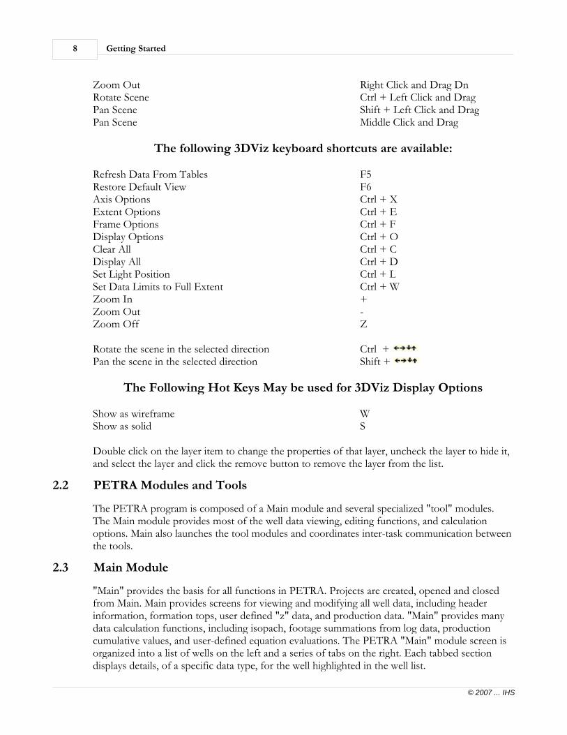
Zoom Out Right Click and Drag DnRotate Scene Ctrl + Left Click and DragPan Scene Shift + Left Click and DragPan Scene Middle Click and Drag
The following 3DViz keyboard shortcuts are available:
Refresh Data From Tables F5Restore Default View F6Axis Options Ctrl + XExtent Options Ctrl + EFrame Options Ctrl + FDisplay Options Ctrl + OClear All Ctrl + CDisplay All Ctrl + DSet Light Position Ctrl + LSet Data Limits to Full Extent Ctrl + WZoom In +Zoom Out -Zoom Off Z
Rotate the scene in the selected direction Ctrl + Pan the scene in the selected direction Shift +
The Following Hot Keys May be used for 3DViz Display Options
Show as wireframe WShow as solid S
Double click on the layer item to change the properties of that layer, uncheck the layer to hide it,and select the layer and click the remove button to remove the layer from the list.
2.2 PETRA Modules and Tools
The PETRA program is composed of a Main module and several specialized "tool" modules.The Main module provides most of the well data viewing, editing functions, and calculationoptions. Main also launches the tool modules and coordinates inter-task communication betweenthe tools.
2.3 Main Module
"Main" provides the basis for all functions in PETRA. Projects are created, opened and closedfrom Main. Main provides screens for viewing and modifying all well data, including headerinformation, formation tops, user defined "z" data, and production data. "Main" provides manydata calculation functions, including isopach, footage summations from log data, productioncumulative values, and user-defined equation evaluations. The PETRA "Main" module screen isorganized into a list of wells on the left and a series of tabs on the right. Each tabbed sectiondisplays details, of a specific data type, for the well highlighted in the well list.

PETRA Tutorial Overview 9
© 2007 ... IHS
In the "Main" module, there is a drop down menu called "Tools". You can open the variousmodules "Tools" using this menu. There are icons that can be used to open most of the modulesand icons for navigating through the wells, refreshing data in the tables, and highlighting a wellon the map.
The "Icons" above are "Create New Project", "Open An Existing Project", "Close The CurrentProject", "Select Wells By Data", "View/Edit Zone Data", "Mapping", "Cross Section", "SpreadSheet", "Log Cross Plot", "Z Cross Plot", "Histogram", "Mo Production Analysis", "2DSeismic", "PetraSeis 2D-3D Interp", "Thematic Mapper", "3d Visualizer", and "Slip LogsModule", "Help", and "Close and Exit".
NOTE: The "PetraSeis 2D-3D Interp" and "Thematic Mapper" icons will not be shown untilthose modules have been installed.
Click on the "Create New Project" icon to start the "Create New Project" Wizard. You willbe guided through the necessary steps to create a new project or to connect to an existing sharedproject.
A "Create New PETRA Project" dialog screen will be displayed.
NOTE: (This option is not available with the DEMO version of PETRA)
Click on the "Open An Existing Project" icon to display a list of projects that are availablefrom the local "Parms" path. The local "Parms" path is the path on the local PC where PETRAwas installed, typically, C:\geoplus1\parms.
Click on the "Close The Current Project" icon to close the current project in preparation toclose "PETRA", "Create New Project", or "Open An Existing Project". NOTE: Close any openmodule before closing the current project. This allows you the opportunity to save your"Overlay" data in the "Map" and "CrossSection" modules if you've made any changes. If thereare any open modules when you click on the "Close The Current Project" icon, a "Close OpenModules" dialog screen will be displayed.
You can click on the "OK" button and close each open module, or you can click on the "Cancel"button to let "PETRA" close the open module along with the associated tables. If you click onthe "Cancel" button, a "Closing PETRA Modules" dialog screen will be displayed.
If you've made a change to an overlay layer, you will still have to either save the overlay file ordismiss the save of the overlay file.
Click on the "Select Wells By Data" icon to display the "Select Wells By Data" dialog screen.

Getting Started10
© 2007 ... IHS
You will be able to select a set of wells based on the "Search Criteria" that you select.
Click on the "View/Edit Zone Data" icon to bring up the "View/Edit Zone Data" dialog screen.You can select data from the "FMTOPS" or "WELL" zone to view and edit.
The "Icons" above are "Highlight Well On Map", "Refresh Data From Disk", "Display PreviousWell In List", "Display Next Well In List".
When the "Map" module is open, you can click on the "Highlight Well On Map" icon toshow the well that you are on in "Main" with a green highlight circle around the well symbol andthe cursor will be pointing to the highlighted well. If you double click on a well in the "Map"module, you will be returned to the "Main" module with that well selected. If the well is not inthe "Selected Well List" in "Main", an "Information" dialog screen will be displayed:
"You will be returned to the "Main" module, but the well that you doubled clicked onwill not be shown."
2.4 Mapping Tool
The "Mapping" tool provides PETRA mapping functions, including base maps, contour maps,bubble maps, and attribute maps. "Maps" provide a direct link to the well database by doubleclicking on a well. "Maps" also provide many data editing functions, including modifying orspotting well locations from footage calls, importing and modifying land grids, and capturing andmodifying contours. The "Mapping" tool also functions to define the wells for a cross sectiondisplay.
2.5 Cross-Section Tool
The "Cross-Section" tool displays profiles across the project area and can include deviated boreholes, well logs, formation tops, faults, posted well information, cored, perforated and testedinterval indicators, and overlays of user-drawn interpretations. The "Cross-Section" tool offersmany data editing functions, including interactive correlation of formation tops, digital log dataediting and depth shifting, and picking "high-low" cutoffs used for log normalization. In additionto digital logs, depth calibrated raster images can be displayed on the cross section.
The cross section can be displayed as a "structural" or a "stratigraphic" section.
"Production Charts" and "Attribute" symbols can also be displayed.

PETRA Tutorial Overview 11
© 2007 ... IHS
2.6 Spread Sheet Tool
The "Spread Sheet" tool provides a quick way to view and edit selected columns of data for a fewwells or for all wells in the project. Each data column is chosen from the well header items,formation tops, and Zone data items. Tops can be edited as measured or subsea TVD. The"Spread Sheet" tool provides a find and replace function for making global changes.
A "CSV" file can be exported from the "Spread Sheet" tool with options to include the columnheadings and to include the "WSN" column.
2.7 Log Cross Plot Tool
Log cross plots are traditionally used by petrophysicists to analyze relationships between digitallog curves and to develop models for log transformations. PETRA can generate XY, XYZ, andternary cross plots for a single well or multiple wells combined. Additional "discriminator" logcurves can be specified to filter the data. Standard graphs and charts can be overlain on the crossplot to differentiate lithologies. Polygons can be digitized onto the cross plot and utilized inadvanced log transformations to develop facies log curves.
2.8 Z Cross Plot Tool
The "Z Cross Plot" tool is similar in functionality to the log cross plot tool except tops and zonedata (numeric and dates) are cross-plotted.
2.9 2D Seismic Tool
The "2D Seismic" tool offers the user the ability to import 2D and 3D seismic locations andhorizon "z" data. Line names and shot point numbers can be edited. Shot point Z data ispresented in tabular format and can be viewed and edited on a shot point or line basis.
2.10 Log Histogram Tool
The "Log Histogram" tool displays both a statistical histogram and a vertical log curverepresentation of a selected log curve, and allows the user to visually "pick" values such as highand low picks, that can be used elsewhere in PETRA. These picks are typically used for digital log

Getting Started12
© 2007 ... IHS
curve normalization.
2.11 Production Analysis Tool
The "Production Analysis" tool provides monthly production data for cross-plotting and declinecurve analysis functions. Parameters, such as projected reserve estimates, can be computed bygraphically fitting exponential or hyperbolic functions to decline curves and capturing and storingrelated parameters in the database for mapping and other purposes.
2.12 PetraSeis Tool
The "PetraSeis" tool is sold separately and designed to be tightly integrated with PETRA.Therefore it is launched from the "Main" module of PETRA, similar to the other PETRAmodules. Typically a project requiring interpretation of 2D seismic lines and 3D seismic volumeswill have associated well and land grid data, and IHS recommends the project map projectionand well header data be loaded prior to loading the seismic data. Following this sequence willease the work flow and minimize confusion. For details on loading well, log curve, andcartographic data into PETRA, please refer to the appropriate sections in this Manual. Includedwith your PetraSeis license is a sample project dataset, called the SoonerDemo Project. All of thenecessary files will be installed in PETRA and PetraSeis to allow you to practice interpretation ofthe data.
2.13 Thematic Mapper
PETRA's "Thematic Mapping" module is designed to import, display, query and coloring ESRIShape Files based on its attribute data and send the results to the Mapping Module's overlaylayer.
The primary functions of the Thematic Mapper are:
· Read in a shape file as a "theme" with associated attributes.
· Create new shape files resulting from expression, spatial or distance queries applied to theshape file's attributes.
· Create a "Well Theme" using the PETRA well data such as well header information,formation tops and zone data items.
· Coloring a theme based on "single symbol", "unique values" or "class breaks".

PETRA Tutorial Overview 13
© 2007 ... IHS
· Copy, clip and re-project a theme.
· Send a theme to a layer in the "Map Module's" overlay.
· Create and export a "WSN" list file from a "Well Theme".
***** IMPORTANT *****This module requires the installation of ESRI's Map Objects 2.2. PETRA will attempt toinstall it automatically when you select the Thematic Mapping menu or icon.
***** The Map Objects run-time install program, available on our Web site ***** is notbeing deployed with "alldisks" or "petraup" update files. It's simply too large. It is beingdeployed with the "server" and all CDs. The MO run-time install program should bedownloaded into the "Petra system" folder, ie, "PetraSrv" for network installs or"geoplus1" for standalone installs. The MO run-time install file can be downloaded fromthe IHS web site at: "http://www.geoplus.com/ftp/mo22rt.exe". The MO run-timelibrary is about 35 MB in size.
2.14 3d Visualizer
3DViz Module is one of the latest enhancement to PETRA. This tool is designed to begeologically based, and since it is tied directly to the PETRA database, it is extremely easy todisplay well (straight and directional boreholes, tops, digital logs, perfs, shows), subsea grids,isopach, PETRA map overlays, and cross section "panels". It is easy to zoom in and out, rotateand shift the display, control the position of a light source (for surface shading), and print theresult or capture an image for insertion into other software packages.
2.15 Slip Logs Module
The Slip Log Module allows up to four (4) raster log images to be viewed simultaneously andscrolled independently or locked together. Logs are displayed horizontally across the screensimilar to laying out logs on your desk. Formation tops to be picked or modified from raster logimages. An alignment cursor function allows logs to be aligned and locked by picking a similarfeature on each log or logs can be aligned at a specific formation top. Fault gaps can be displayedon the logs creating blank spaces in raster images as the image below the fault gap is shifteddown in depth.
2.16 Calculations and Transformation Tools
The real strength of PETRA lies in its robust set of calculation and transformation tools. User-defined equations can be evaluated to compute new Zone data, well logs, monthly production, orseismic horizons. Cumulative production can be computed for any data in the monthlyproduction database. Reservoir properties, such as net, gross, net-to-gross ratio, phih, and phiacan be computed from well logs over specific depth intervals and using various cutoff criteria.Simple formation thickness can be computed for multiple zones with corrections for deviatedwells. Structure data can be used to compute true stratigraphic thickness for intervals. Theadvanced log transformations allow the user to write procedures called user models. User modelscontain multi-line arithmetic expressions with Boolean operators and are typically used to

Getting Started14
© 2007 ... IHS
perform multi-well log analysis.
2.17 Units
(A)PETRA assumes a single, consistent unit of measurement for all data in the database. A project's"default" units can be set to FEET (Imperial) or METERS (Metric). Once the default units areestablished, data can be viewed as either Imperial or Metric Units.
(B)Setting the "default" data and depth units involves selecting the "Units>Set Default Units..."menu in Main.
(C)Default units are set for both XY and depth coordinates. XY and Depth units can be set fromthe Map Projections options (Project>Settings>Set Map Projection).
The "XY Coordinates are in" option is used to convert latitude/longitude values to "XYCoordinates" when loading or changing these values. The "XY Coordinates" will be calculatedbased on the projection parameters that have been set.
The "Default Depth Units" option is used when loading Tops and Curve data that do not haveunits assigned to them.
2.18 Help
There are several useful items under the "Help" menu. When you click on "Help..." the helps thatare available in PETRA are displayed from the beginning of the "Help" file. The "Help" file can
be scrolled through using the "Back" button and the forward button.
To take a look at the changes that have been made to PETRA, click on the "What's New..."menu.
2.19 Last
The "Last" menu will keep track of the last ten menu items that you have selected. This is ashortcut that can be used instead of navigating through the other menus for tasks that are usedfrequently.

Data Organization and Concepts 15
© 2007 ... IHS
3 Data Organization and Concepts
This section describes several simple but very important program design concepts, which youshould familiarize yourself with to take full advantage of PETRA.
3.1 PETRA Projects
Review the Chapter below that is titled "Creating a New Project" to learn about creating a newproject and the two data types that a project contains, which are project data and parameter data.Project data consists of all well data, logs, seismic shot points, land grids and any computed data,such as contour grids. Project data can be shared with other team members given access to theproject. Project data may reside on a network drive.
"Private Parameter Data" cannot be shared with other team members. "Private Parameter Data"consists of all settings representing your view of a particular project. Such items as colorpreferences, mapping and cross-section options currently in effect are examples of parameterdata. For single user projects, the project and parameter data can reside entirely on a local ornetwork disk if so desired. Remember to backup your local project and parameter datafrequently. For data that is stored on your network, make sure that the data on the network isbacked up as well.
3.2 Sharing Projects
PETRA project data can be shared among team members.
Your private parameters should not be in the "Shared Project\Parms" folder. They should be in apath that no one else will be writing to. An example would be "Shared Parms\UserName\Shared Project Name".
See the section below titled "Creating a Shared Project".
3.2.1 Creating a Shared Project
Typically, a shared project will reside on a network drive. When the project is first created using
the PETRA Project Wizard, you would select the "Create New Project" option. Next you wouldspecify that the project will be shared. This allows you to establish two separate directories(folders), one for the project data (database files, public parameters, overlays etcetera) andanother for the private or personal parameters.
NOTE: The directories (folders) should not have the exact same path for the project data andthe personal parameters. The personal parameter database cannot be shared with another user.The dialog screens below show the steps to create a new project that will be shared.
When you open PETRA, there is an option to "Create a NEW Project". Click the "Radio"
button to the left of this option.. Click on the "OK" button with the green check .This will start a "Create New PETRA Project" wizard.
Click the "Radio" button to the left of the "Create A New Project" option. Click on the "Next"

Getting Started16
© 2007 ... IHS
button.
Click on the "Radio" button to the left of "Yes - Project will be shared". Click the "Next" button.
Enter the "Name" for the project and the "Description" for the project. Click the "Next" button.
A "Create New PETRA Project" dialog screen will be displayed where you will select thedirectory path for the shared project to be stored on the network. Double click on the uppermost folder where the project is to be created. You will see the path that will be used for theproject. In the example below, the path is: "H:\PETRA Projects". You will see the pathdisplayed above the directory selection area. Click on the "Next" button. (Note: You do not drilldown to a project sub folder).
You will select the directory path for the personal parameters. The personal parameters can bestored on the local machine in the C:\geoplus1\projects folder, however, it is highlyrecommended that you store this information on the network so that the data will be backed upon a regular basis. If you store the information on your local machine, remember to back up thedata on a regular basis. Double click on the upper most folder where the personal parameters areto be stored. You will see the path displayed above the directory selection area. In the example,the path is "T:\Petra Priparms\HLM". (Note: You do not drill down to a project sub folder).Click on the "Next" button.

Data Organization and Concepts 17
© 2007 ... IHS
A "Create New PETRA Project" dialog screen with "Finished." will be displayed along with thepaths for the "Public" (Project Directory), and the Private (Parameter directory) parameters. Youwill see a message "Project Can Be Shared". You should not see the project name duplicated ineither path. PETRA will create the Public and Private project folders along with the tables, filesand project.ini files that are needed for the new project. Click on the "Finish" button.
If you see the project name duplicated, like the examples shown below:
\\Geoplus1\H Drive\TempProjects\Shared_Projects\CREATING A PROJECT\CREATINGA PROJECT or\\Geoplus1\H Drive\Petra PriParms\HLM\CREATING A PROJECT\CREATING APROJECT
you need to click on the "Back" button and follow the procedure outlined above, making surethat you do not select the project name for either of the paths.
Anyone wanting to access the shared project will create a new project. They will first be asked toselect the project to connect with using a directory browser to point to the remote project'sdirectory. Next, the Project Wizard will guide them to setup a "Personal Parameter Folder(Private Parameters Path)" on their local or network drive. A network drive is preferred, as the

Getting Started18
© 2007 ... IHS
network drives are generally backed up on a regular basis. If you chose a local drive, make surethe local project data is backed up on a regular basis.
Click on the "Create a New Project" "Radio" button and then click on the "OK" button with the
green check .
This will start a "Create New PETRA Project" wizard.
They will select the option to "Connect To An Existing Shared Project" and click the "Next"button.
If they use the drop down "drive mapping" button they will drill out to the project anddouble click on the project folder.
If they use the "Browse Network..." button , when they double click on theproject folder, they will need to select the project ".INI" file and click on the "Open" button. Adialog screen like the one above will be displayed. Click the "Next" button.
They will select the directory path for the personal parameters. Read about selecting the personalparameters in the section above. Click the "Next" button.
A "Create New PETRA Project" dialog screen with "Finished." will be displayed along with thepaths for the "Public" (Project Directory), and the Private (Parameter directory) parameters. Youwill see a message "Project Can Be Shared". You should not see the project name duplicated ineither path. PETRA will create the Public and Private project folders along with the tables, filesand project.ini files that are needed for the new project. Click on the "Finish" button.
If you see the project name duplicated in the "Parameter Directory" path, like the examplesshown here:\\Geoplus1\H Drive\Petra PriParms\HLM\CREATING A PROJECT\CREATING APROJECTyou need to click on the "Back" button and follow the procedure outlined above, making surethat you do not select the project name. The project name will be created for you with the defaultprivate parameter files and the project.ini files needed for the shared project.
3.2.2 Shared Project Data is Live
When sharing projects, all concurrent users of the project have immediate access to any and allchanges made by any other user. Since some spread sheet displays contain a local copy of thedata, it may be necessary to refresh the spread sheet to see the latest changes. The main screen
contains a small refresh icon , "Refresh Data From Disk", for this purpose . You will find amenu item in all modules to refresh data. Some modules have an icon that can also be used torefresh the data.

Data Organization and Concepts 19
© 2007 ... IHS
3.3 Project Data
Project data consists of all well data, logs, seismic shot points, land grids and any computed data,such as contour grids. Project data can be shared with other team members given access to theproject. Project data may reside on a network drive.
3.3.1 Unique Well Identifier (UWI)
Each well that is stored in a PETRA project must have a "Unique Well Identifier" or UWI. EachUWI contains from 1 to 20 characters that uniquely identifies the well. Typically for U. S.domestic data, the UWI is the API number for the well. The API number that ends in "0000" isthe original well. Sidetracks and Re-completions of the original well are considered as separatewells in PETRA. The sidetrack is recorded in the 11th and 12th digits and the re-completion isrecorded in the 13th and 14th digits of the API number.
3.3.2 Well Sequence Number (WSN)
The database assigns a unique numeric identifier for each well called the "Well SequenceNumber" or WSN. The WSN is used for data retrieval only and cannot be modified. WSN's arenot reassigned when wells are deleted. A well's WSN is unique for a given project. The same wellin another project will not necessarily have the same WSN.
3.3.3 Well Label
The "Well Label" is a 1 to 32 character data field that can be customized for well identification.Many times, a project will contain several wells with the same well name or number. PETRAprovides the Well Label as a means to create an identifier using all or portions of other well datafields, such as operator, lease name, section-township-range, etcetera. The "Well Label" can becustomized for currently selected wells or for all wells. There is also an option to store thecomputed label in the "Sort Key Field" for the well and is displayed on the "Well" tab in "Main".The default "Well Label" is the "Unique Well Identifier".
3.3.4 Zones
PETRA provides for an unlimited number of user-defined data fields to be stored in the projectdatabase. User-defined well data are organized into groups called "zones". A zone is like a tablecontaining one or more columns of numbers, dates, or text. Rows in the table correspond towells.
Zones have a corollary with geologic zones by the fact that they are defined by a depth interval.Zones can be referenced to measured depths, subsea TVD, but are more frequently referenced toformation markers or tops. When a zone references an upper and lower formation marker,PETRA can quickly evaluate the tops to determine the appropriate depth interval for any givenwell.
The Zone database provides a logical and efficient organization for managing geologicalmappable well data. Items such as isopach, TST, net pay, average porosity, etcetera, can begrouped together under the zone corresponding to the depth interval of interest.
Many functions within PETRA can process several zones at once. For example, you can compute
Getting Started20
© 2007 ... IHS
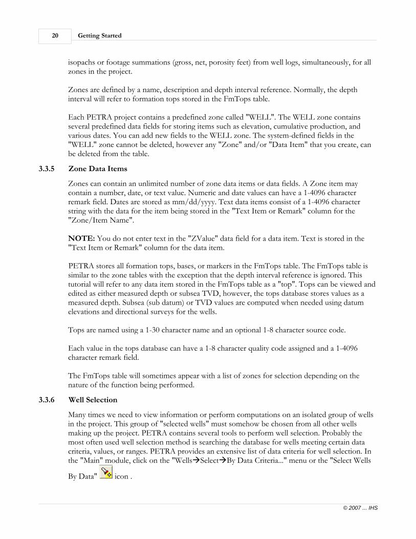
isopachs or footage summations (gross, net, porosity feet) from well logs, simultaneously, for allzones in the project.
Zones are defined by a name, description and depth interval reference. Normally, the depthinterval will refer to formation tops stored in the FmTops table.
Each PETRA project contains a predefined zone called "WELL". The WELL zone containsseveral predefined data fields for storing items such as elevation, cumulative production, andvarious dates. You can add new fields to the WELL zone. The system-defined fields in the"WELL" zone cannot be deleted, however any "Zone" and/or "Data Item" that you create, canbe deleted from the table.
3.3.5 Zone Data Items
Zones can contain an unlimited number of zone data items or data fields. A Zone item maycontain a number, date, or text value. Numeric and date values can have a 1-4096 characterremark field. Dates are stored as mm/dd/yyyy. Text data items consist of a 1-4096 characterstring with the data for the item being stored in the "Text Item or Remark" column for the"Zone/Item Name".
NOTE: You do not enter text in the "ZValue" data field for a data item. Text is stored in the"Text Item or Remark" column for the data item.
2PETRA stores all formation tops, bases, or markers in the FmTops table. The FmTops table issimilar to the zone tables with the exception that the depth interval reference is ignored. Thistutorial will refer to any data item stored in the FmTops table as a "top". Tops can be viewed andedited as either measured depth or subsea TVD, however, the tops database stores values as ameasured depth. Subsea (sub datum) or TVD values are computed when needed using datumelevations and directional surveys for the wells.
Tops are named using a 1-30 character name and an optional 1-8 character source code.
Each value in the tops database can have a 1-8 character quality code assigned and a 1-4096character remark field.
The FmTops table will sometimes appear with a list of zones for selection depending on thenature of the function being performed.
3.3.6 Well Selection
Many times we need to view information or perform computations on an isolated group of wellsin the project. This group of "selected wells" must somehow be chosen from all other wellsmaking up the project. PETRA contains several tools to perform well selection. Probably themost often used well selection method is searching the database for wells meeting certain datacriteria, values, or ranges. PETRA provides an extensive list of data criteria for well selection. Inthe "Main" module, click on the "WellsàSelectàBy Data Criteria..." menu or the "Select Wells
By Data" icon .

Data Organization and Concepts 21
© 2007 ... IHS
For example, PETRA easily handles complex queries such as: find all wells which have a porositylog, cum gas production greater than 1000 mcf and total depth greater than 9000 feet, andcompleted after 01/01/1990. Well selection lists can be saved to a disk file and reloaded whenneeded.
Each PETRA module, i.e., "Map", "Cross Plot", etcetera, contains its own list of selected wells.Wells selected in the "Main" module are those wells displayed in the well list and is the defaultwell list for other modules.
3.3.7 Missing or "Null" Data Values
PETRA displays a missing or "null" value as a blank field. Therefore, to set a value to null, simply
blank out the value and click the "Save" button.
3.4 Creating a New Project
This section illustrates how to create a new PETRA project and import ASCII "Tabular" welldata and log curves from LAS files.
New Project Overview
PETRA projects typically store all data relevant to a particular geographical area. The ProjectName is used to build the directory path on both local and network hard drives. Projects consistof two data types, project data and parameter data. Project data consists of all well data, logs,seismic shot points, land grids and any computed data, such as contour grids. Project data can beshared with other team members given access to the project. Project data may reside on anetwork drive. Parameter data consists of all settings representing your view of a particularproject. Such items as color preferences, mapping and cross-section options currently in effectare examples of parameter data. For single user projects, the project and parameter data canreside entirely on a local or network disk if so desired.
During PETRA installation, a "PROJECTS" directory is created under the installed programdirectory (GEOPLUS1 by default). Unless you will be sharing project data with others, it ishighly recommended that you create all PETRA projects under the "PROJECTS" directory path.
Directory paths need not already exist prior to creating a new project. You can type in a non-existent path structure and PETRA will create all sub-directories for you.
New projects can be created from Main's "ProjectàNew…" menu.
Any currently opened project must be closed prior to creating a new project. When ready tocreate a new project, select the "ProjectàNew..." menu, in the Main Module. This will invokethe "Project Setup Wizard" or from the "Welcome" dialog box when you first log into PETRA,click on the "radio" button to the left of "Create a NEW Project" to invoke the "Project SetupWizard".
When the "Project Setup Wizard" starts, it will guide you through the project setup process.

Getting Started22
© 2007 ... IHS
You can "Create A New Project" or create the necessary directory links to "Connect To AnExisting Shared Project". Click on the appropriate "Radio" button. For this example, we will usethe "Create A New Project" option. Click on the "Next" button.
New projects can be designated as shared or non-shared. Shared projects are typically setup on anetwork drive and have the project database stored in a different directory than the privateparameter data. Click on the "Radio" button to the left of "Yes - Project will be shared". Click onthe "Next" button.
Project Name And Description
The project name is used to identify the sub directory name for project and parameter data paths.Enter a descriptive acronym for the project. Windows 2000/XP/Vista directory names maycontain blanks and can be longer than the old 8-character DOS names. The project description isused as a title for identification on graphical displays and can be modified after the project iscreated. Click on the "Next" button.
Project Database Directory Path
The project database path defines the directory path where the shared project data will reside.This directory will contain the bulk of the project's data so choose a drive with sufficient space. Ifthe project will be shared among team members, you should select a network drive. Click on the"Next" button. The path can be drive letter that has been mapped or the UNC path can be used.For instance, the example shown below is a drive letter mapping path. "H:\Petra Projects". Anexample of the UNC path would be "\\geoplus1\h drive\Petra Projects".
Personal Parameters Directory Path (Shared Projects Only)
The parameter data path defines the directory path where you want your own parameters storedfor a shared project. If the project is not shared, the parameter directory will be the same as theproject database directory. The path can be drive letter that has been mapped or the UNC pathcan be used. For instance, the example shown below is a drive letter mapping path."T:\PetraPriparms\HLM". An example of the UNC path would be"\\geoplus1\t drive\PetraPriparms\HLM".
Click on the "Next" button.
The information for the project is displayed on the "Finished" dialog screen. The project nameshould never be repeated twice for the "Project Directory" or the "Parameter Directory". If yousee the project name twice, click on the "Back" button and re-select the upper folder where theproject is to be created or the upper folder where the private parameters are to be created.
After completing the new project wizard, the new project's database will be created and theproject will be initialized with default values. The main screen will display a single "Project" Tab.Only a few options are available until wells are added to the project. Since this is a new project,the "Projection" for the project has not been set. You will see a message letting you know thatyou should set the projection for the project. Click on the "Yes" button.

Data Organization and Concepts 23
© 2007 ... IHS
To set the projection, click on the "ProjectàSetting...àSet Map Projection..." menu. Select theappropriate projection for the project.
To load data into the project, click on the "ProjectàImportà" menu and select the appropriateimport option for the data that you have to load into the project.
NOTE: You should set the projection, then load the well data into a project before attempting toload cartographic data.
To add "Wells" manually, click on the "WellsàAdd A New Well..." menu. You will enter eachUWI (API number), then click on the various tabs to fill out the various data fields. Typically,however, wells are added by importing well data from either one of the commercial data suppliersor from simple "tabular" ASCII files by clicking on the "ProjectàImportà" menu.
3.4.1 Importing Well Data
PETRA provides several options for importing well and other data into a project database. Theimport options are located under the "Project" menu on the main screen. If you have anotherproject, you can export data in the "PETRA Project File (*.PPF)" format and load that filedirectly into the new project. We have a "PETRA ASCII Well Data File" that is a publishedformat for data to be loaded directly into PETRA as well. This format is used by several dataproviders and is the preferred format when obtaining data from a vendor. TheprojectàImportàGeneral Well Data From…" menu includes options for importing data fromseveral different sources which are listed below.
Well Data and Tops
· Generic ASCII File (Function key "Ctrl+T"). This is a tabular file consisting of well dataformatted so that each well occupies a row or file record and each data field is a column.Sometimes called a "Spreadsheet" and is user defined. NOTE: We cannot load a ".XLS"file format.
· IHS 297 (PI) Well Data (Fixed or Comma) which is commercial well data IHS's CD-ROM software or on-line service. This file format is Y2K compliant.
· Old PI 97 or 197 Download (Fixed Field) NOTE: We highly recommend using the 297Well Data File as these files are not Y2K compliant.
· Geological Data Services-II, (GDS-II File), which is Well Data and Formation Topsfrom Geological Data Services.
· GES Wellbase ASCII vers. 2, which is an exported ASCII file format from Geographix.· Tobin WCS, which is basic well header and location information.· NRIS - Okla. Geol. Society (WHFF) File, which is well data from Oklahoma Geological
Survey.· Geological Consulting Services, a GCS File, which is Formation Tops from Geological
Consulting Services.· Dwights WDS file, which is the Dwights Well Data System CD-ROM download format.· Landmark 3x Metafile, which is an ASCII file that contains well data exported from
Landmark and other systems.· Landmark Standard 29 Format, which is an ASCII file which contains well data exported

Getting Started24
© 2007 ... IHS
from Landmark and other systems· Landmark OWX File, which is an ASCII file which contains well data exported from
Landmark and other systems.· QC Data Axxses DPDT Request Format File.· IOG Red Top (Kansas Data Format File)· PI 98 Production File, (Comma Delimited), (IHS 298 is recommended as it is Y2K
compliant), from which a limited amount of Well Header Information can be loaded.· SEISX Well Data File· DrillingInfo "DR" File (V2)· IHS Dwight's Narrative Report· Lasser V2 File· P2ES Dir Survey Data·
3.4.2 Importing Tabular ASCII Well Data
On the Main Screen, under the "Project" Menu, there is an "Import" option for bringing datainto PETRA. One of the many options under the "General Well Data From…" menu item is the"Generic ASCII File..." option, sometimes referred to as a "Spreadsheet" file. We do not load".XLS" files into PETRA, however you can save the file out as a comma separated variable file,".CSV", or a space delimited text file from your spreadsheet program.
ASCII well data files contain data fields in columns, similar to a table or spread sheet. PETRAcan import files containing more than one record per well; however, all wells must contain thesame number of records. Header records or column identifiers can be skipped over if necessary.One column must contain the UWI or API number. Other data columns can contain well headerinformation, such as well name, operator name, producing formation, etcetera. In addition, datacolumns can be imported into any of the project's zone data items or formation tops.
Select the "ProjectàImportàGeneral Well Data From…àGeneric ASCII File" main menu.Click the "Import File" Tab, then click the "Open File" button and select the "sample_well.txt"file located in the ...\GEOPLUS1\PROJECTS\Tutorial folder.
Click on the "Open File" button to locate the data file to load into your project.
Select the "sample_well.txt" file located in the ...\GEOPLUS1\PROJECTS\Tutorial folder.
Click on the "Data Format" tab. When PETRA opens the file the first two data records aredisplayed in a scrollable box in the Data Record section of the Data Format screen.
The start and end column position and record number identifies each column of data to beimported. The columns can be selected from the lower data record by "swiping" the columnusing the mouse. Swiping is accomplished by clicking the left mouse button at the startingposition of the column. While holding the left button down, drag the mouse to the end columnof the field and release the left mouse button. The "Start Column" and "End Column" fields willshow the columns containing the data. The selected column must then be associated with either awell header or zone data item from one of the two drop down lists. The associated column is

Data Organization and Concepts 25
© 2007 ... IHS
then added to a list of "Field Definitions" by clicking the "Add" button . Since we have aheader record in the data file, we need to tell PETRA to skip the header record when the data is
loaded. Click on the first actual data record, then click on the "Set Skip" button .
There are over 200 predefined data items that can be entered into your project using the uppermost drop down data item list. Additional data items (numbers, dates, text strings) can be definedby the user.
A format file for the sample_well.txt has been provided to show the data items and associatedcolumns the data is located in. To load the format file, click on the "Load..." button, and selectthe "sample_well.FM1" file. This file is located at the root of the Tutorial project.
Click on the "Open" button. You will see the data items and associated data columns that havebeen defined for the input data file. Once you have selected the data items and columns for thefile that you are loading, you can create a template file to be used for another file that containsthe same data items located in the same columns.
Data can also be loaded from a ".CSV" file. Instead of columns, the data items are defined as a"Field Number" instead of defined columns. An example file called "sample_well.csv" is locatedin the ...\GEOPLUS1\PROJECTS\Tutorial folder. The format file is called"sample_well_csv.FM1" and is located in the same directory.
Click on the "Options" TAB to observe the options that are available when importing data froma tabular file. For this exercise, we will accept the default to "Add New Wells and UpdateSelected Wells".
Click on the "Locations" tab to observe the options that are available when importing locationsfrom a tabular file.
Finally, after all columns are selected and the appropriate options are chosen, click the "OK"
button with the green check to initiate the import process.
3.4.3 Importing Digital Log Data
Importing LAS Data
Digital well log data can be imported from industry standard LAS formatted files.
Select the "ProjectàImportàLogs FromàLAS File" menu option on the main screen to importa LAS file.
Choose the LAS file from the ..\GEOPLUS1\PROJECTS\Tutorial directory called"sample.las".
Since LAS files contain log data for a single well, PETRA will attempt to match the currentlyselected well with the header records of the selected LAS file. If the currently selected well is not

Getting Started26
© 2007 ... IHS
the well that is in the ".LAS" file, an "Information" dialog will be displayed if the well exists inthe project.
You will receive a "Warning" message if a match cannot be found in the project to the"UWI/API" that is in the ".LAS" file.. In this case you should use the "Target Well" button toselect the well that you want to load the LAS logs into, or select a file that contains the"UWI/API" for the well in the project that the curves need to be loaded into.
For the "sample.las" file, the well is in the project and is automatically selected as the "TargetWell".
The "LAS Header Information" lists all identifying data from the LAS file header records. Thelog curves, available for loading, are listed in the "Select Logs To Import" section. Click tohighlight the logs you want to import or click on the "All" button to select all of the curves in thefile and click on the "Import Logs" button with the green check. The "DEPT" log contains thedepths for the curves and is not a curve that is to be imported.
Log curves can be imported under a different name from the one specified in the LAS file. LASlogs can be renamed as they are imported. To rename a log, click to highlight the log name in the
"Select Logs To Import" list. Then click the "Rename" button and type the new logname. If the new log name does not already appear in the log database, you will be prompted forthe new log name's units and description. The new name will then be added to the logdefinitions, even if no data is ever loaded. After entering the "New Log Name", click on the"OK" button.
Enter the "Description" for the new log name.
The curve name on the "Import LAS Log Data File" dialog screen will be changed to the newname. The curve will have to be reselected. Hold down the "Ctrl" key and click on the new curve
or click the "All" again to reselect all of the curves.
Click on the "Depths" tab.
Click on the "Restrict Depths..." button to display the "Set Depth Range"dialog screen.
The depth range screen allows the upper and lower depths of an interval to be defined usingeither a constant depth value (Measured Depth or TVD Subsea Depth) or variable depth basedthe formation tops.
"FM Top" and "Offset From Top" - This option allows the depth interval to vary from well towell based on the values of the formation tops. Select the formation top reference from the dropdown list and optionally set a numeric offset value. The offset provides for such intervals as 100feet above and below a given top.
We will accept the defaults. Click on the "OK" button with the green check to close

Data Organization and Concepts 27
© 2007 ... IHS
the "Set Depth Range" dialog.
You can decimate the log data as it is imported by loading every nth depth sample. Set the "N="field to 1 to load all samples. Set the value to 2 to load every other sample, 3 for every 3rd sample,and so on.
Click on the "Options" tab.
The "Radio" button options are:
· The "Add or Replace Logs" option simply adds the log if no other log with the same namefor the well exists, or replaces the current database log if one already exists.
· The "Add New Logs Only" option will not over write existing data and only stores theimported log if another log with the same name for the well does not exist.
· The "Merge Into Existing Logs" option adds the log if it doesn't exist and merges itself withthe any existing log of the same name. Use the merge option to combine multiple runs ofthe same logs over different depth ranges.
· The "Add or Rename" option will add the log if no other log with the same name for thewell exists. If there is a log with the same name, the incoming log will be renamed with a"_1" appended to the existing name to give it a new name.
The "Check" box options are:
· "Enable Sample Rate Round Off Correction Algorithm" will correct for depth round offerrors caused by a sample rate (step) value that is an irrational number such as 0.1524. E.g.,log data digitized with a sample rate of 0.5 feet, then written to an LAS file as meters maycause round off errors in the depth values depending on the algorithm used by the datasupplier or digitizing company. PETRA can correct round off if you select to load the entiredepth range of curve data and the data has no missing depths. Click the "Enable SampleRate Round Off Correction Algorithm" check box to activate this option.
· The "Disable Error Scanning and Repair" option was added to scan for potential badcharacters in the curve data and looks for data that is not space delimited. These conditionsare corrected if this option is checked.
· Choose the "Interpolate Missing Depths" option if the LAS file includes gaps in the depthsand you want to interpolate values over the missing intervals.
· Choose the "Remove Special Characters From API Number" options to remove any non-numeric value from the API number in the LAS file. Embedded blanks are converted tounderscores prior to matching wells in the database.
· "Scan Depths and Use Minimum Sample Rate Found" scans the depths and determines theminimum sample rate if this option is checked.
· The "Append Following Source To Curve Name (Blank For None)" allows you to add asource to the curves being loaded.
Click on the "Import Headers" tab.

Getting Started28
© 2007 ... IHS
You can import information from the "LAS Header Data" by highlighting the item in the "LASHeader Data" column and selecting the appropriate item from the "Well Data" drop down list orfrom the "Zone Data" drop down lists. After making the choice, click the "Add To List" button.After making the selections you would click on the "Imports Headers" button with the greencheck. For our example we will not use this option.
If there are tops in the LAS file, they can be loaded by clicking on the "Import Tops" tab. Thetops will be selected and the "Import Tops" button with the green check will be clicked. The topswill be loaded into the database. We do not have any tops in this sample file.
Click back on the "Options" tab and click on the "Import Logs" button tobegin importing the log curves.
After the curves are loaded, the following confirmation message will be displayed. If you haveanother LAS file to import, you can click on the "Yes" button and import the log data for thenext well. For our exercise, click on the "No" button.
Go to the "Logs" Tab, click the "Refresh Data From Disk" icon to get the latest list of logsfor the well. Click on "WSN 2", then click on the "Logs" tab. Click on a log to highlight it orhold the "Ctrl" button and left click to select more than one log curves. Click the "Log Preview"
button to view the selected logs.
LAS BATCH IMPORT
You can import more than one LAS file at one time by using the "Import Logs From...àLASBatch Import..." menu.
You would click on the "Explorer..." button or the "Browse..." button to locate your LAS files.You would select all of the LAS files that you wanted to load at one time, then click on the"Open" button. After you have the LAS files selected, you would review the "Options" tab and"Depth" tab to set the parameters that you want to use. After you have chosen the options for
this import, click on the "Import Logs" button to begin importing the logcurves. The import batch process will cycle through each of the LAS files until all of the fileshave been processed.
3.5 Project Menus
There are many settings that can be made to customize your project. We will examine each ofthese settings that can be set by Clicking on the "Project" menu in the "Main" module. The"Project" menu is located in the upper left hand corner of the "Main" screen.
3.5.1 Project>Remarks File Menu
The "Remarks File..." option uses Notepad to open a file where you may store any ASCIIinformation about the Project. The file is named "REMARKS.TXT" and is located in thePARMS folder for the project.

Data Organization and Concepts 29
© 2007 ... IHS
3.5.2 Project>Import Menu
The "Import" option is used to load data for the project and is discussed in detail in the varioussections of the manual where data loading is mentioned
There are lots of options for loading general well data into PETRA.

Getting Started30
© 2007 ... IHS
3.5.3 Project>Export Menu
The "Export" option is used to create a "PETRA Project File" (*.PPF) or a "PETRA TemplateFile" (*.PTF). Data from the various tables can be exported as well. There are options to createan ASCII Tabular Well Data File, an ASCII Tops File, a Zone Data file, two Landmark files, LogCurves, Raster Logs (TIF files) and LIC files from the current project to a selected file folder,Directional Survey Data, Top Definitions and a SCA – MCS Z Data, GES Wellbase V2, andPETRA ASCII Well Data to LogSleuth. Monthly Production Data can be exported as a Tabularfile, a Production Analyst file, or a More Simulator Recurrent Data file.

Data Organization and Concepts 31
© 2007 ... IHS
3.5.4 Project>Close Menu
The "ProjectàClose Project" menu option can be used to close the current project withoutclosing "PETRA", and retaining your license.
You can also use the "Close The Current Project" icon in the "Main" module.
3.5.5 Project>Reopen Menu
The "ProjectàReopen" menu option displays the last five projects that have been opened. Withthe left mouse button, click on the project that you want to open.

Getting Started32
© 2007 ... IHS
3.5.6 Project>Settings Menu
The "ProjectàSetting…" menu option is used to customize your project by setting the "MapProjection" and various options in "Program Options...". You can "Password" protect yourproject, reset a module that may have some problems, set the "MJ LogSleuth Project", etcetera.
3.5.6.1 Program Options...
Customizing the settings for the current project is accomplished by clicking on the "Main"module's "Projectà Settingsà Program Options" menu. A dialog box will be shown that hastabs to display various options that are available for the current project.
3.5.6.2 Set Map Projection...
Click on the "Main" module's "Projectà SettingsàSet Map Projection..." menu to bring up the"Map Projection Settings" dialog screen.
The map projection settings determine how Latitude-Longitude coordinates are converted toX,Y coordinates for display purposes. If your project contains only X,Y locations, choose the'No Projection - Locations are in XY' option. If you are not sure which projection to use or don'treally care, choose the Polyconic Projection. Polyconic works well except very near the equator,in which case choose UTM.
Click on the "Help" button for assistance with the various settings.
3.5.6.3 System Colors...
The user can customize all graphics elements, such as borders, titles, screen background,etcetera. Screen color and plotter color for each element can be selected independently froma palette of 16 solid colors. Line thickness and style (solid, dashed, dotted, etcetera) can alsobe selected for each element. Customization of the system colors can be accessed via the"Main" module's "ProjectàSettingsàSystem Colors" menu. Also, colors for individualmodules can be changed from the "DisplayàColors" menu of the module.
3.5.6.4 Well Symbols...
This option displays the symbols that have descriptions assigned to use in your projects. Theyare displayed on the left side of the dialog screen in the section titled "Current WellDescriptions". The total number of symbols available to you in PETRA are displayed in theright display panel, titled "Symbol Definition" under the section titled, "Available Symbols".Currently, there are 185 symbols available to chose from.
To change the color or description for a Well Symbol, click on the symbol in the CurrentWell Descriptions portion of the dialog screen. The Symbol Code, current description,Screen Color, and Plotter Color are displayed in the Symbol Definition portion of the dialogscreen. Change the current information for the selected symbol and then click on the"Apply" button.
To add a Well Symbol to the Current Well Descriptions:

Data Organization and Concepts 33
© 2007 ... IHS
· Click on the New Description button.· Type in the Symbol Code that you want to use in the Symbol Code data field. You can use
up to a maximum of eight characters for the Symbol Code.· Type in a description in the Description data field. You can use up to 60 characters for the
description. Click on the color for the Screen and Plotter Color Selection.· Scroll down the list of Available Symbols and click on the one that you want to add.· Click on the "Apply" button. The new symbol will be added to the bottom of the Current
Well Descriptions list.
· Click on the "OK" button with the green check .
To drop a Well Symbol from the Current Well Descriptions list:· Click on the "Symbol" in the "Current Well Descriptions" list that is to be dropped.· Click on the "Drop Description" button. That Well Symbol will be deleted from the
current list.
· Click on the "OK" button with the green check .
3.5.6.5 Reset Module...
This option is used to reset a module that has become inoperable.
You may want to save some parameter files before you reset the module. For instance, whenyou "Post Well Data ", you can save a template that can be reloaded after resetting themodule so you don't have to re-build your data posting template. The saving of the parameterfile may not be called a template for each option. As an example, the "Attribute Map" usesthe term "Settings" instead of "Template". For each option that you have data beingdisplayed on the map, save your settings or template if you want to recover those parametersafter resetting the module.
Click in the check box next to the module that you want to reset. Click on the "OK" button.
The message that is displayed below will be shown.Click on the OK button.
The selected module has been set to the defaults for that module. Any settings that you mayhave entered will need to be re-entered.
You can re-load the individual setting or template files for each option that you saved thefiles for. Do not load a saved "Map Settings File".
3.5.6.6 Reset Default UWI Column Widths
This options resets the columns to the right of the "WSN" column on the "Main" screen.
3.5.6.7 Project>Exit Menu
The "ProjectàExit" menu option can be used to close the current project and exit PETRA.
Other options for closing a project and PETRA are provided by clicking on the "PETRA" logo

Getting Started34
© 2007 ... IHS
in the upper left corner and selecting "Close" on the dialog screen, or by clicking on the "X" inthe upper right corner, or the "Close and Exit" icon that looks like a door.
When the "Exit geoPLUS" message is displayed. Click on the "OK" button.
If this "Close Open Modules" dialog screen is displayed instead, you have the option of clickingthe "OK" button which will allow you to close each of the open modules, or you can click on the"Cancel" button to have "PETRA" close each of the open modules. This latter option is useful ifyou have used "Task Manager" to close one of the modules.
3.5.6.8 Project>Prospect Menu
The "ProjectàProspect" menu option is used to create a prospect well list, load a prospect welllist, or to change the wells from "Prospect" mode to "Project" mode. When in "Project" mode,all of the wells for the entire project will be used. There is a "Help" section for "Prospects".
3.5.6.9 Help
The "Help" menu displays the information available for "Prospects".Click on "ProjectàProspectàHelp..." menu to display the "Prospects Help" dialog screen.
The "PETRA Help" dialog screen is displayed. Click and drag the "Scroll" button to view theremaining information in the "Prospects" help screen.

Main Module 35
© 2007 ... IHS
4 Main Module
Review the "Main" module in the "PETRA Tutorial Overview" chapter above to understand themanagement of project data and how to access the other modules.
4.1 Switching Between Modules
Each PETRA module is an executable program in communication with "Main" and other activemodules. Each module appears in the Windows task bar and can be accessed by clicking themodule task bar icon. An example of the "Start Bar" is shown for Start, Quick Launch Tool Bar,Task Bar items; Main Module, Map Module, Cross Section Module, and the Icon Tray for XP:
Each module also contains a "Window" menu from which any active module can be accessed.The screen shot below shows the menu from the "Cross Section" module. By clicking on"WindowàMain", you will be returned to the "Main" module.
The "Window" menu from the "Map" module is shown below. When you click on"WindowàCross Section", you will be returned to that module. To return to the "Main" module,click on "WindowàMain".
4.2 Opening the "Tutorial" Project
Click on the "Start" button for Windows . A "Pop Up" menu with choices will be
displayed. Click on "All Programs" , then "Petra" ,
, then "GeoPlus Petra"
.
A shortcut is created on your desktop to run PETRA. The PETRA Demo icon looks like this:
, The full evaluation icon look like this: When you can double click on theappropriate icon. the PETRA splash screen will be displayed briefly. Wait until it disappears.

Getting Started36
© 2007 ... IHS
If this is the first time that you have opened "PETRA", the following message will be displayed:
Click on the "OK" button to continue.
The "Welcome to PETRA" dialog screen will be displayed. Click on the "Radio" button to theleft of the "Open an Existing Project".
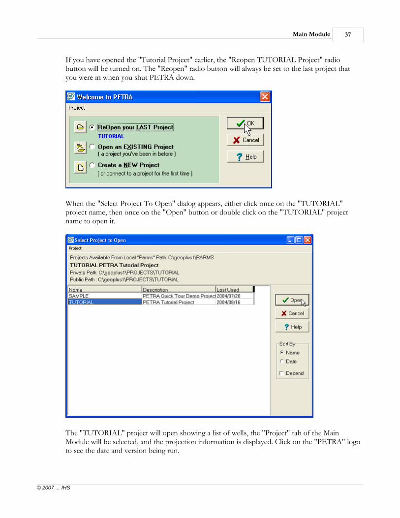
Main Module 37
© 2007 ... IHS
If you have opened the "Tutorial Project" earlier, the "Reopen TUTORIAL Project" radiobutton will be turned on. The "Reopen" radio button will always be set to the last project thatyou were in when you shut PETRA down.
When the "Select Project To Open" dialog appears, either click once on the "TUTORIAL"project name, then once on the "Open" button or double click on the "TUTORIAL" projectname to open it.
The "TUTORIAL" project will open showing a list of wells, the "Project" tab of the MainModule will be selected, and the projection information is displayed. Click on the "PETRA" logoto see the date and version being run.

Getting Started38
© 2007 ... IHS
4.3 Main Module Overview
The PETRA "Main" module screen is organized into a list of wells on the left, and a series oftabs on the right. Each tabbed section displays details of a specific data type for the wellhighlighted in the well list.
Typing over the data displayed in the data entry fields will modify any data in the tabbed sections.
Each tabbed section contains a "Save" button , or an "Update" button , whichmust be clicked to update the database with any changes that are made. PETRA automaticallyprompts you to save the data if you change data then click the left mouse button on another wellor attempt to close the project without saving the changes.
4.3.1 Projection for Projects
The projection for the project should be the first setting made before loading any data into theproject.
Well locations are provided as either latitude-longitude or x-y coordinates. The followingdiscussion on map projections is meant only to ensure your projects are set up correctly based onwhether you have lat-lon or x-y data. It is not meant to explain the differences in the various mapprojections or datum's. Click either the Main Module's "Projectà Settingsà Set Map
Projection" menu option or from "Project" tab, click on the "Set Map Projection" button ,

Main Module 39
© 2007 ... IHS
or on the "Location" tab, click the "Projection" button to display the "MapProjection Settings" dialog screen.
PETRA operates in one of two coordinate modes. All well locations, seismic and other locationdata, are stored as Latitude-Longitude or as X-Y coordinates. You cannot have some wells withlat-lon and other wells with only X-Y values. When lat-lon locations are stored, PETRAcomputes the X-Y coordinate corresponding to the selected map projection. When X-Y locationsare stored, PETRA computes the Lat-Lon coordinate corresponding to the selected mapprojection, which has to be correct for the X-Y coordinates that are loaded. Several industrystandard map projection algorithms are provided, including: Polyconic, UTM, TransverseMercator, Lambert Conformal Conic, and Albers Conical Equal Area. Each projection is bestsuited for certain areas of the world. In addition, a "State Planes" look-up table is provided forstandard mapping in the US. If you do not know or do not care what map projection is used foryour lat-lon values, try using the "Polyconic" projection option. Click the "Set By Data Limits" toset the appropriate parameters, based on the actual project data. The "Polyconic" projectionworks well in project areas located between 20 and 60 degrees latitude.

Getting Started40
© 2007 ... IHS
After setting the Projection Parameters for the Project, it is a good idea to lock the projectionparameters. Locking the Map Projection will prevent the projection from being changedinadvertently by anyone accessing the project.
If you have x-y well coordinates, and don't know the correct projection for the x-y coordinates,you need to set the map projection type to "No Projection - Locations are in XY". Noconversion will be done on the well coordinates.
NOTE: If you've made any changes to the projection, in the Sample or Tutorial projects,click the "Cancel" button, as we do not want to change the map projection at this time.
4.4 Sorting the Well List
The well list displays the well sequence used by the database, the unique well identifier (typically,the API number), and the custom well label. Try scrolling the list left and right to see thedifferent fields.
The well list can be sorted by the UWI, WSN, Well Name, or Well Label. The default sort orderis by WSN. Position the mouse cursor over the well list and click the right mouse button todisplay the pop up sort menu.
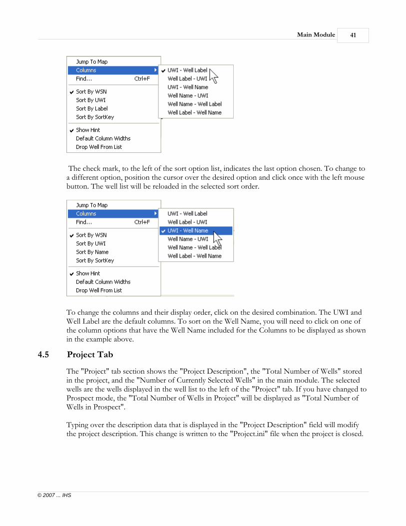
Main Module 41
© 2007 ... IHS
The check mark, to the left of the sort option list, indicates the last option chosen. To change toa different option, position the cursor over the desired option and click once with the left mousebutton. The well list will be reloaded in the selected sort order.
To change the columns and their display order, click on the desired combination. The UWI andWell Label are the default columns. To sort on the Well Name, you will need to click on one ofthe column options that have the Well Name included for the Columns to be displayed as shownin the example above.
4.5 Project Tab
The "Project" tab section shows the "Project Description", the "Total Number of Wells" storedin the project, and the "Number of Currently Selected Wells" in the main module. The selectedwells are the wells displayed in the well list to the left of the "Project" tab. If you have changed toProspect mode, the "Total Number of Wells in Project" will be displayed as "Total Number ofWells in Prospect".
Typing over the description data that is displayed in the "Project Description" field will modifythe project description. This change is written to the "Project.ini" file when the project is closed.

Getting Started42
© 2007 ... IHS
Click on the PETRA logo to display information about PETRA.
This is the same dialog that is show when you click on the "HelpàAbout PETRA..." menu.

Main Module 43
© 2007 ... IHS
Click on the "X" in the upper right corner of the dialog screen to close the "About PETRA"dialog screen.
4.6 Well Tab
On the "Main" dialog screen, click the mouse button on the tab labeled "Well".
The "Well" tab shows the well header detail information for the well highlighted in the well list.The screen includes data fields for: unique well id (UWI), well number, well name, operator,label, lease name, lease number, etcetera.
By pulling the main screen wider, you will see a button called "Zone Favorites", when clicked,you can select and display information from other tables on this screen. For instance, you coulddisplay the KB, DF, GR, TD, and Completion Date from the Well table. You would see the datavalues that are stored in the table displayed in this area.
You can change to a different well by clicking the mouse on the well list in the "Unique Well ID"
column or by clicking the "Next" and "Previous" buttons, or by clicking the
"Previous Well", "Next Well" buttons located to the right of the UWI display data field.
Typing over the current value will modify any of the well data fields. As you type, the "Save"
button will become active, indicating you have the option to update the database withyour changes. After making all necessary changes to the "Well" tab screen, click the "Save"
button . If you modify any data fields and attempt to go to another well without firstsaving the data, PETRA will prompt you to save the data.
If you click the "Save" button but realize you made a mistake, click the "Undo" button
to reset the well to the values prior to the last save. To see how this works, select the firstwell in the well list and change the historical operator name by typing; "Big Oil Company" in the
"Hist Oper" field. Now, click the "Save" button . If you have a sound card enabled on
your system, you will hear a sound as the data is updated. Next, click the "Undo" button .The well data will reset to the prior values.
The well symbol displayed on maps and cross sections is shown on the "Well" tab screen.Choosing one of the symbols listed in the "Well Symbol and Desc" list box will change thesymbol. There are currently 185 symbols to choose from. Again, you will need to click the "Save"
button to store your changes.
The "Active Datum" list allows you to choose a datum elevation from several predefined fieldsincluding; Kelly bushing (ELEV_KB), derrick floor (ELEV_DF), ground level (ELEV_GR), andseismic datum (ELEV_SEIS). The datum elevation is used to compute "subsea" formation topsor other depths at run-time. Each well can reference a different elevation. The actual elevationdata values can be viewed and edited on the "Zones" tab screen, where the datum elevations are

Getting Started44
© 2007 ... IHS
listed under the "WELL" zone; on the "FmTops" tab, where the datum elevation is shown abovethe tops, and on the "Well" tab in the Active Datum" data field.
The "Remarks" section, on the "Well" tab, provides a place to store any general comments abouta well. This section is also used to store various remarks imported from commercial well datasources.
4.6.1 Adding a New Well Manually
NOTE: New wells cannot be added to the "Demo" version of PETRA and you cannot create anew project in this version.
Wells can be added manually to a project using several methods. From the "Well" tab screen youcan add a well by typing a new UWI and all associated well header information then click the
"Save" button . PETRA will detect the attempt to change the UWI and display the "Addor Replace Well" screen. At this point, you can click the "Add New Well" button
to add the new well to the database.
Try adding a new well. Change the first well's UWI field from 42201077770000 to
42201077771000. After changing the value, click the "Save" button . The followingscreen will appear. Click the "Add New Well" option. The new well will appear at the end of thewell list.
Wells can also be added using the main screen's "WellsàAdd A New Well" menu.

Main Module 45
© 2007 ... IHS
You will be prompted for the UWI for the new well. Enter the new UWI and press OK toactually add a new well into the database.
Shown below is the dialog screen for entering the API number for this menu item. We will notactually enter this API into the well database. Click on the "Cancel" button
You can add more wells by entering more UWIs or click the "Cancel" button when done. If youactually add a well, you will see the last well "UWI" that was added at the bottom of the dialogscreen. The well list will be repositioned to the last well added to the project. You can thenupdate the well header fields for each of the newly added wells.

Getting Started46
© 2007 ... IHS
4.6.2 Changing the Unique Well Identifier
Changing the unique well identifier for a well is done from the "Well" tab screen. Type over the
UWI field and click the "Save" button . You will be prompted with the "Add or ReplaceWell" screen. Click the "Replace" button to change the UWI for the selected well.
This time change the UWI field of our new well from 42201077771000 to 42201077771001. Atthe "add or replace" prompt, click the "Replace" button. The new well will be updated with thenew UWI. To see the change in the display, you may need to click on the well above and thenback on the new well. This causes the database tables to be refreshed.
Try replacing the UWI with that of another well. Notice that PETRA will not allow two wellswith the same UWI. Click on the "OK" button to close the "Error" dialog screen.
4.6.3 Deleting a Single Well
You can delete a single well from the database using the "WellsàDelete Well…" menu item.First, click on the well list to highlight the well you want to delete. Select the new well we addedin the last section. Then, pull down the Wells Menu and click once on the "Delete Well…" menuitem. You will be prompted twice to verify that you really want the well and all of its data deletedfrom the database. After deleting the well, the screen will reset to the "Project" tab showing thenumber of wells in the project. It will show a total of 21 wells and 21 wells selected. Our newwell is no longer in the well list.
4.6.4 Deleting Multiple Wells
NOTE: Read through the following section, but do not actually delete the "Tutorial" wells fornow.
To delete more than one well at a time, first select the wells to be deleted using one of the wellselection tools such as the "WellsàSelectàWells By Data Criteria" menu item. Then choose the"WellsàDelete All Selected Wells" menu item.
CAUTION: this option will delete all of the wells displayed in the well list on the left sideof the "Main" screen.
However, you will be prompted twice to verify that you really want to delete these wells. Afterdeletion, the screen will reset the "Project" tab to show the number of wells in the project and allremaining wells in the project will be selected.

Main Module 47
© 2007 ... IHS
NOTE:Always make sure that you have the correct wells selected that are to be deleted beforeusing this option.
4.7 Location Tab
From the "Main" screen, click the mouse button on the tab labeled "Location".
When there is directional survey data for the well you will see "Directional Survey Available"listed in the "Misc Location Information" data area.
The location screen displays the well's surface and bottom hole latitude-longitude and X-Ycoordinates. You also have access to region-specific, detailed-location data using a series ofbuttons located on the right side of the screen. Detail screens are provided for "DirectionalSurvey Data", "Section-Township-Range Data", "Offshore Location Information" (Gulf ofMexico Data), "Texas Location Data", "North East Location Data", and "Projection Settings"(Map Projection Data).
4.7.1 Deviated Wells
Directional or deviated wells are wells that contain directional survey data describing thecoordinates of the borehole at various depths. PETRA queries the database for the presence ofdirectional survey data to determine whether or not a well is deviated. Directional surveys can beimported or entered by hand as either MD, TVD, Dip and Azimuth, or as MD, TVD, X-offsetand Y-offset. The radius of curvature method is applied to convert dip and azimuth to x and yoffsets.
Deviated wells are treated differently than non-deviated wells. For example, during mapping, adeviated well's symbol location is determined by projecting the deviated borehole path onto themap surface. The well symbol is positioned along this path at a predetermined depth. This depthcan be the total depth of the well or a depth of a formation top. The surface projection of theborehole is sometimes referred to as a "worm track" or "spider diagram". On cross sections, thedeviated path of the borehole is projected onto the plane of the cross section. Digital log curves,tops, and tests are plotted relative to the angled borehole.
4.7.2 Displaying the Survey Data
Click the well list on the well with WSN=17. This is a directional well as indicated by the remark"Directional Survey Available" in the "Misc Location Information" section. Next, click the "DirSurvey" button on the "Location" tab to access the survey data details.
The survey screen contains a series of tabs. The "General" tab shows remarks and provides autility to convert depths from measured depth to TVD and visa versa.
Click on the "Data" tab. This section shows the survey data in spreadsheet format. The data canbe added or modified from this spreadsheet.
Click on the "Preview" tab. A graphical representation of the survey data is plotted. On the left isa graph showing the East-West and North-South components of the survey footage offsets fromthe surface location. The "y" axis is TVD and can be adjusted by changing the "Max Depth" field

Getting Started48
© 2007 ... IHS
and clicking the "Redraw" button. The right-hand graph shows a map view of the survey "worm"or "spider" plot. The axes are in feet (or optionally, meters) on the earth's surface.
The "Import/Export" tab allows the data to be imported from or exported to an ASCII file.
Click the "Cancel" button to close the survey screen without making any updates to thedatabase.
4.7.3 Locking Projection
Click either the Main Module's "Projectà Settingsà Set Map Projection" menu option or from
"Project" tab, click on the "Set Map Projection" button , or on the "Location" tab, click the
"Projection" button to display the "Map Projection Settings" dialog screen.
Click on the "Lock" tab, click on the "Map Projection Settings" dialog screen, then click on the"Lock Map Projection..." button. You will click on the "OK" button on the "Lock MapProjection?" confirmation screen and then on the "OK" button on the "Information" screen thatis displayed.
4.7.4 Locking Locations
To lock the locations for the wells, you will click on the "ProjectàSettings…àProgramOptions…" menu. The "PETRA Program Options" dialog screen will be displayed.
Click on the "Locks" tab. Click the "Check Box" to the left of "Well Location Locking Enabled".Click on the "Lock All Locations..." button.
Click on the "OK" button.
Click on the "OK" button with the "green" check at the bottom of the "PETRAProgram Options" dialog screen. When you click on the "Locations" tab, the locations will bedisplayed in "Red" and a message will be displayed in the "Misc Location Information" field thatstates that all of the locations are locked at the project level.

Main Module 49
© 2007 ... IHS
4.8 Fm Tops Tab
From the "Main" screen, click the mouse on the "FmTops" Tab.
PETRA stores all formation tops, bases, fluid contacts, or markers in the FmTops table. Thistutorial will refer to any data item stored in the FmTops table as a "top". Tops can be viewed andedited as either measured depth or subsea TVD, however, the database stores all tops as ameasured depth. Subsea (subdatum) or TVD values are computed when needed using datumelevations and directional surveys.
The "Active Only" Check Box allows you to display only those Formation Tops that have livedata in them. This is useful when you have a large number of top names for the project, butmany of the tops have not yet been picked.
The "FmTops" tab displays a table showing all formation tops for the highlighted well. The tableshows both measured depths (MD) and TVD subsea depths. You will notice the datum elevationused to compute subsea values is displayed at the top of the table. The deviated wells aredisplayed with a column header of TVDSS. Non deviated wells have a column header of SS. Ifthe well is deviated, the subsea values are also TVD computed from directional survey data. Youcan modify either the "MD" or "TVD" value. The other value will be changed accordingly. Youcan also change the "Active Datum" and/or value from the "FmTops" Tab. You must click the
"Save" button to update the database.
IMPORTANT: When typing values in the data cells, the value is recorded only when you movethe cursor out of the edited cell or when the Enter key is pressed. The cursor moves out of a cellwhen an arrow key or the tab is pressed. To set a value to null, highlight the value, press the

Getting Started50
© 2007 ... IHS
delete key or space bar then press the "Enter" key. Both MD and TVD values should show ablank cell.
A top's remark field can be edited by typing in the "Remarks" cell or by using a "Edit Remarks"dialog box. The "Edit Remark..." dialog box is activated from a right button click pop up menuClicking on the "Edit Remark..." option brings up a "Remarks" dialog screen where you can addor modify the remarks for the top. Clicking on the "Edit Properties..." option brings up a"Modify Zone Item Description" dialog screen which allows you to change the "Item Name","Source", "Units (<>Metric)", number of "Decimals", "Description" and "Remarks" for the"Item".
NOTE: Remember to click in a data cell for the top that you want to edit.
Formation tops are identified by a 1 to 30 character "Item Name" and a 1 to 8 character "Source"identifier sometimes referred to as a "Source Code". The "Source" identifier is optional. Ageologist might use their initials as the "Source" to identify their own picks for a particular top.
Each individual top value can have a 1 to 8 character quality code to indicate the "quality" of theformation pick. In addition, each top value can contain a 1 to 4096 character remark field.
The "FmTops" tab screen contains several buttons along the bottom for "Maintenance", Printingthe tops for the selected well, adding a new top, setting up aliases, setting a display order for thetops, and showing tops by a specific source.
4.8.1 Printing Tops
The "Print Tops" button provides the ability to print the tops for the currently selected well.Click on the printer icon to display the printer dialog menu to choose the printer and print thetops. Click "OK" to print to the selected printer.
4.8.2 New Top
The "New Top…" button allows you to quickly add a new top definition to thedatabase.
4.8.3 Top Aliases
The "Aliases" button provides a mechanism to specify a prioritized list of top names asformation top equivalencies. During mapping, for example, if an alias name is specified, thedatabase will use the alias list to search the database for the first top value that does not contain a"null" value. To set up an alias, first click the mouse in one of the data cells of the top to bealiased. Then, click the "Aliases" button.
NOTE: When defining aliases, don't forget to select the aliased top as the first top in thealias list.

Main Module 51
© 2007 ... IHS
4.8.4 Show Tops By Source
The "Show Tops By Source" button displays a dialog screen called, "Show Tops BySource", and is used to show the tops with all sources or by a selected set of tops. There is anoption to sort the tops by name.For this project there are not any source codes for tops. Click the "OK" button with the green
check or the "Cancel" button with the "Red X" to close this dialog screen.
4.8.5 Reordering Tops
The "ReOrder" button allows the geologist to specify the display order for viewingtops in a particular order or stratigraphic sequence. There is an option to display only those topsspecified in the "Order List". When this option is turned on, the other tops will not be displayed.This feature can save you time trying to find a particular top name in a long list of tops. There aretwo sort buttons available at the bottom of the Reorder Dialog Screen. An "A to Z" button and a"Z to A" button. On the "Import/Export" Tab, there are two options to save a file or read a filein to specify the sort order. The "PETRA Order List" is a binary file. The "External File (StratTable)" is an ASCII file that can be edited by any editor that can open an ASCII file, such asNotepad, Excel, Word, etcetera. When using Word or Excel remember to save the file as a textfile instead of a Word Document or an Excel Spread Sheet.
4.8.6 Formation Tops – Maintenance
The "Maintenance" button invokes the maintenance dialog screen. This dialogscreen provides maintenance of both tops and zone data. To perform maintenance on tops, clickon the "Zones" tab, then select "FMTOPS" in the "Zone Name" data field. Click on the "DataItems" tab.
After clicking on the "Maintenance" button click on the "Data Items" tab. Thereare several options available to assist in the maintenance of the Tops.
· The "New Item…" button will bring up a dialog box for adding a new "Data Item" toFMTOPS.
· The "Modify Item…" button is used to modify any of the "Data Items" "Data Fields".· The "ReOrder…" button is used to order the "Data Items" in the order desired by the
user.· The "Clear Data…" button is used to clear all of the "Data Fields" for the selected "Data
Item".· The "Clear Remarks…" button is used to clear the "Remarks" field for the selected "Data
Item".· The "Delete…" button is used to delete the selected "Data Item".· The "# Decimals…" button is used to set the number of decimals to be displayed for the
selected "Data Item(s)".· The "ALL" button is used to select all of the "Data Items".· The "None" button is used to de-select any/all selected "Data Items".· The "Save File" button creates a CSV file with the Project name and description along
with the top names and description.

Getting Started52
© 2007 ... IHS
· The "Save Template..." button saves a template definition file.· The "Load Template..." button loads a saved template definiton file. It will add zone item
names to the current zone.· The "Print" button prints the Project name and description along with the top names and
description.· The "Hilite Color..." button with the crayons is used to select a color for high lighing the
selected item and the one with the large "X" is used to rempve the hilite color for theselected items.
· The "Value Count" button is used to display the number of wells that contain live datafor each of the "Data Items". Shown in parentheses to the left of the "Formation TopName" in the dialog screen above.
4.9 Zones Tab
From the "Main" screen, click the mouse on the "Zones" tab.
PETRA provides for an unlimited number of user-defined data fields to be stored in the projectdatabase. User-defined well data are organized into groups called "zones". A zone is like a tablecontaining one or more columns of numbers, dates, or text. Rows in the table correspond towells.
Zones have a corollary with geologic zones by the fact that they are defined by a depth interval.Zones can reference measured depths, subsea TVD, but more frequently reference formationtops or markers. When a zone references an upper and lower formation marker, PETRA quicklyevaluates the tops to determine the appropriate depth range for any given well.
The Zone database provides a logical and efficient organizational tool for managing geologicalmappable well data. Items such as isopach, true stratigraphic thickness, net pay, average porosity,etcetera can be grouped together under the zone corresponding to the geologic depth interval ofinterest.
The "Zones" tab section of the main screen provides a quick visual reference for "system" and"user" defined zone data fields. Zone data are presented as a table with a list of zone names onthe left and data values on the right. Clicking on the zone name results in the zone data itemsbeing displayed for the selected zone. Zone data values can be edited and updated to the
database by clicking the "Save" button .
A zone item's remark field can be edited by typing in the remark cell or by using a "EditRemarks" dialog box. The "Edit Remarks..." and "Edit Properties..." dialog box are activatedfrom a right button click pop up menu:

Main Module 53
© 2007 ... IHS
Click on the "Edit Remark..." option to bring up a "Remark" screen where you can add ormodify the remarks for the zone.
Click on the "Edit Properties..." option to bring up a screen which allows you to change the itemname or description.
The "Jump To Hyperlink..." option is used to associate a file or WEB Link that you would like tosee displayed for the well when you active this option. For instance, you could enter the path toan excel spreadsheet in the "Text Item or Remark" data field. When you click on the "Jump ToHyperlink..." option, the specified spreadsheet would be displayed.
Click on the "Default Column Widths" option to set the column widths back to the defaultwidths.
Click on the "Lock Item for This Well...", or using the "Hot keys" "Ctrl+L", to bring up aconfirmation dialog allowing the item to be locked.
Click on the "Unlock Item for This Well...", or using the "Hot keys" "Ctrl+U", to bring up aconfirmation dialog allowing the item to be unlocked.
Click on the "Lock Item for Selected Wells...", or using the "Hot keys" "Alt+L", to lock the itemfor all selected wells.
Click on the "Unlock Item for Selected Wells...", or using the "Hot keys" "Alt+U", to unlock theitem for all selected wells.
A zone "Maintenance" utility can be accessed for adding, deleting, and modifying zonedefinitions and zone data variables.
The "View/Edit All…" button invokes a screen which provides viewing andediting of zone data items presented by zone instead of by well. A table shows the zone data forall selected wells. A statistical histogram is available showing the data range and frequencydistribution for zone data. The view/edit utility can be accessed from various PETRA screensand provides a quick data check or verification of computed results.

Getting Started54
© 2007 ... IHS
4.9.1 Creating a New Zone
A zone is a logical grouping of related data. Zones usually represent a geologic interval andreference formation "tops" to define the depth interval of interest. Zones contain "z" data itemsor variables for storing numbers, dates and text fields. When you add a new zone to a project youonly add the definition and depth reference. You are not adding any data values to the wells.
Suppose we have two formation tops, "A" and "B", which define the upper and lowerboundaries of our zone of interest. We can create a zone called "AB" to store reservoir propertiessuch as isopach, net pay, porosity feet, etcetera.
First, click the "Maintenance" button on the "Zones" Tab. The "ZoneMaintenance" screen will be displayed.
· The "New Zone…" button will bring up a dialog box for adding a new Zone.
· The "Modify Zone…" button will bring up a dialog box for modifying theZone name, Description, and/or remarks.
· The "Delete Zone…" button will delete any non-system defined Zone that isselected to be deleted.
· The "ReOrder" button allows the geologist to specify the display order forviewing tops in a particular order or stratigraphic sequence.
Click on the "New Zone" button . On the new zone definition screen, enter "AB"as the zone name. Enter a description such as, "Interval A to B". Click the "OK" button to addthe zone definition to the database. The zone "AB" has been added to the database. Next, weneed to define the depth interval for the "AB" zone. The "Interval Definition" Tab is activated.The upper and lower depth references can now be set.
Set the upper depth to FmTop "A" by selecting top "A" from the drop down list in the "UpperDepth" group. Click the radio button labeled "FmTop" to set it to the on position ("Radio"button filled in), if it is not already set. Next, set the lower depth to the FmTop "B" in a similarmanner. Again, make sure the radio button labeled "FmTop" is set to the on position ("Radio"button filled in). Notice too, that you can enter offset footages for the UPPER and LOWERdepths. This allows the zone to start, for example, 25 feet (or meters) above or below thespecified formation top. Click the "OK" button. An Update Zone Interval definitionconfirmation screen is displayed with the Zone name, the Upper Depth FmTop, Lower DepthFmTop, and offsets for each if entered.
Click OK to return to the "Zones" Tab screen. You will receive a prompt upon exiting for eachzone that has been modified. Click "Yes" to accept the changes. The "AB" zone will be added tothe "Zones" Tab. Click on the "AB" zone name. You will notice that there are no data fieldsassociated with the new zone. In the next section we will add data fields to the new zone.

Main Module 55
© 2007 ... IHS
4.9.2 Adding New Zone Variables or "Items"
Zone data items are added to a zone using the zone "Maintenance" button locatedat the bottom of the "Zones" Tab screen or by using the "Add a new Zone…" button
.
We will use the zone "Maintenance" button to add the Data Items to the Zone.
From the Zone Maintenance Screen, click to highlight the "AB" zone name, then click the "DataItems" Tab.
If any data items have been added, they will be displayed at this time. We will create three zonedata items. Click the "New Item" button to start adding fields using the "New Zone Data Item"screen.
Enter the name and description for the data item. For now, enter the name "ISOPACH" anddescription "Interval Thickness". You can specify the units as "FT". Make sure the "Data Type"
is numeric. Click the "OK" button with the green check to add the isopach definitionto the "AB" zone.
The "New Zone Data Item" screen will reappear to allow you to continue entering items. Add afield called "PAY" for "Net Pay" and "PHIH" for "Porosity Feet". Click the "Cancel" button
with the red X to stop adding more data fields.
Return to the "Zones" Tab screen from the maintenance screen by clicking the "OK" button
with the green check .
Click the "AB" zone on the "Zones" Tab list to show the newly added data fields. All values willbe set to null, which is indicated by blank data cells.
New zone variables are also added to zones during calculations. For example, instead of adding

Getting Started56
© 2007 ... IHS
the "ISOPACH" data item definition ahead of time, we could simply compute the "AB" zoneisopach using the "ComputeàFrom ZonesàIsopach" menu option. We could actually create anisopach variable for all project zones at once if necessary.
4.10 Logs Tab
From the "Main" screen, click the mouse button on the tab labeled "Logs" and then click on thewell list to select the well with WSN=10.
PETRA provides a log curve database for storing digital well logs. Logs can be imported instandard LAS and LIS data formats. PETRA includes a robust set of tools for editing, analyzing,and extracting reservoir properties, such as, net pay and hydrocarbon pore volume from log data.
The "Logs" tab section lists the digital well logs stored for a particular well. In addition, if youclick on the "Radio" button to the left of "Values" and double click on a curve, "DPHI" forinstance the log data values for the selected log will be displayed. The log values can be editedfrom this list if desired. If you click on the "Radio" button to the left of the "Curve" option, thelog curve will be displayed.
The "Delete" button will delete the highlighted logs from the selected well.
The "Rename" button allows a selected log to be renamed to one of the alreadydefined log names. Renaming a log for a well simply changes the log name reference.
The "Log Maintenance" button is used to add new log names and descriptions,make global changes to the log database, and rename or delete log curves by name.
The "Depths" button allows you to restrict the depth interval of the data shown inthe "Log Preview" and "Digits" displays.
The "Log Preview" option displays selected well logs side-by-side and is intended as aquick quality control tool. The log preview utility also offers several log editing tools and candisplay and correlate formation tops.
For now, select one or more log curves from the "Logs" tab screen and click the "Log Preview"
button to view the logs. Notice that as you move the mouse over a log curve how the"Status" bar at the bottom of the screen displays the curve summary information. If you click theright mouse button over a specific curve, you will see a large pop up menu containing severalfunctions for editing curves.
Exit the "Log Preview" screen using the "FileàClose" menu or by clicking the standard
Windows "Close" button in the upper right corner of the screen.
When you right click on one of the curves, a Pop Up Menu, as shown below, is displayed. Todiscover more about these options, Click on the "Logs" Tab on the "Main Screen". Click on the"Log Preview" Tab, then on the "Help" Menu.

Main Module 57
© 2007 ... IHS
Another method to display "Help" information for "Log Preview" is to click on the "Help"Menu Item in the Main module. Click on the "Index" Button. A "Help Topics: "PETRA Help"dialog screen is displayed. Type in "Log P" in the available entry field. Double click on the LogPreview entry or click on the "Display" Button at the bottom of the screen.
4.11 IP Tests Tab
From the "Main" screen, click on the "IP Tests" tab. Shown below are the "IP" tests for "WSN"2.
The "Show Combined Well Completions" check box will show the completions from the othercompletions for the well if there are any.
The "Locked" check box will lock the data so that it cannot be modified unless you "Unlock" thedata.
Click on the "Details..." button .

Getting Started58
© 2007 ... IHS
You can add, delete, update, scroll through tests, add IP Test depths to perfs and clear the data
fields on this screen. Click on the "Close" button with the green check to close the"Production Test Details" dialog screen.
4.12 Fm Tests Tab
From the "Main" screen, click on the "Fm Tests" tab. We do not have any "Fm Test" data forthis set of wells.
The "Show Combined Well Completions" check box will show the completions from the othercompletions for the well if there are any.
The "Locked" check box will lock the data so that it cannot be modified unless you "Unlock" thedata.
Click on the "Details..." button .
You can add, delete, update, scroll through tests on this screen. When you click on the"Recoveries" tab, you can add, delete, update, and scroll through "Recovery Details" as well.There is a "Clear Fields" button to clear the data fields. Click on the "Options" tab to uncheckthe "Display Choke Size in 64th inches". Click on the "Maintenance" tab to use the variousmaintenance options, like "Delete All Tests For This Well...", "Delete All Test For ALL WELLSIN DB..." and to "Set All FmTests UNITS FLAGS to Current Project Units".
Click on the button with the green check to close the "Production Test Details"dialog screen.
4.13 Cores Tab
From the "Main" screen, click on the "Cores" tab. Click on the first well in the project. You willsee the data that has been loaded for this well.
Click on the "Details" button .
The "Show Combined Well Completions" check box will show the completions from the othercompletions for the well if there are any.
The "Locked" check box will lock the data so that it cannot be modified unless you "Unlock" thedata by clicking the "Locked" check box to remove the check.
You can add, delete, update, and clear Cored data on this screen. Click on the buttonwith the green check to close the "Cored Intervals Details" dialog screen.
4.14 Perfs/Shows Tab
From the "Main" screen, click on the "Perf/Shows" tab. Click on "WSN" 19 in the project. Youwill see the data that has been loaded in this well for both Perfs and Shows. The "Locked" checkbox will lock the data so that it cannot be modified unless you "Unlock" the data by clicking the

Main Module 59
© 2007 ... IHS
"Locked" check box to remove the check.
Notice that there are two "Locked" check boxes. One for "Perfs" and the other one for "Shows".
Click on the "Perfs Details..." button .
You can add, update, delete the current perf, and clear data. There is a button at the bottom fordeleting all of the perf data for this well. You can also lock the perfs for this well by clicking the"Check" box to the left of "Locked" at the bottom of the screen. If the depths are not sortedproperly, you can sort them by clicking on the "Sort" button at the bottom of the screen.
There are different "Perf Types" that can be set by clicking the "drop down" selection button to
the right of the "Perf Type" data field. Click on the "Cancel" button with the red "X"to close the "Perfed Intervals" dialog screen.
Click on the "Show Details..." button.
You can add, update, delete, and clear data. There is an option for setting the "Shows" byclicking the check box to the left for the type of show or shows that are associated with the depthrange that was entered for the show.
You can mark a show as "Do Not Plot" by clicking the "Check" box to the left of the "Do NotPlot" option at the bottom of the screen.
You can lock the shows by clicking the "Check" box to the left of the "Locked" option at thebottom of the screen.
You can close and accept any changes made by clicking on the "OK" button with thegreen check, or you can close the dialog without saving the changes by clicking on the "Cancel"
button with the red "X".
4.15 Production Tab
From the "Main" screen, click on the "Production" tab and then click the well list to select wellwith WSN=10. For this display the "Mo Prod Chart BkGnd" color has been changed from blackto white. The "Mo Prod Years" color has been changed from white to black. Some of the "MoProd Chart's" colors were changed to make them brighter for the display.
The system colors can be modified by going to "ProjectàSettings...àSystem Colors...". Becareful when making changes to the "System Colors". Remember the original setting so that youcan change the setting back to the original if this causes problems.
PETRA includes a production database for storing production data (or any other data) on amonthly basis. Production can be imported from commercial sources such as IHS, loaded fromASCII tabular files, or entered manually into a custom spreadsheet that is saved as a CSV file and

Getting Started60
© 2007 ... IHS
loaded into the Production table. The database is not limited to OIL, GAS, and WATERproduction. Like the zone database, you can define and store monthly data for an unlimitednumber of data items. Data items, such as, injected water or CO2 production can just as easily bestored, charted, and used in calculations. Functions are available to compute cumulative valuesand perform month-to-month data transformations using a user-defined mathematical equationevaluator.
The "Production" Tab screen shows a chart of selected monthly production data for the currentwell. Wells not containing the selected data are indicated by the words "No Data" in the chart. By
default, Oil, Gas, and Water are displayed in the chart. The "Options" button allows any monthly data to be charted. Scales can be set automatically or manually.
The "Data" button displays the monthly production custom spreadsheet where datacan be entered, modified, and printed.
The "Maintenance" button is used to add, modify, and delete production data itemnames.
4.15.1 Computing Cumulative Production Data
Monthly production data is stored as individual monthly values in the database. If we want toknow and map the total production for the wells in our project, we need to compute a"cumulative" value. The cumulative values are stored in a zone data item, normally under theWELL zone. PETRA can compute cumulative values for any monthly production variable over aselected date range. In addition, we can compute the total number of years used to determine thecumulative values. The total year's value can aid in determining the significance of the productionof one well relative to another well with a similar cumulative value.
The cumulative production calculations are performed for all wells currently selected in the mainmodule, i.e., those wells listed on the main screen.
Select the Main screen's "Compute àFrom ProductionàCumulative Production Rates…"menu.
IMPORTANT NOTE: Year 0 stores any production prior to the first year containing monthlyvalues. These pre-monthluy values are known as "historical values".Click on the "Compute Values Using Following Monthly Production Stream" drop down
selection button and select the data stream that you want to compute the average production
Main Module 61
© 2007 ... IHS
rate for. For our example, we will use "Oil". Make sure the check box beside the "IncludeHistorical (Year 0)" is checked. It's okay if the "Use Aliases" check box is checked. We don'thave any aliases assigned at this time.
Click on the "Time" Tab.
The options that are available provide you with a wide selection for computing values from theproduction data streams.
The "Compute for Constant Date Range" option uses the "From" and "Through" sections todefine the date range for selecting monthly data for the cumulative calculation.
The "Compute for Zone Date Range" option uses the "From Zone Item" and "Through ZoneItem" sections to define the date range for selecting monthly data for the cumulative calculation.You must have a "date" item with a date stored in the database to use this option.
The "Compute for Months" option is used when you want to use a range of months.
The "Compute for First" option is used when you want to compute for the first range of monthsbased on whether they are "producing" or "producing and non producing". There are 2 dropdown selection menus.
The "Compute for Last" option is used when you want to compute for the last range of monthsbased on whether they are producing or non producing. There are 2 drop down selection menus.
For our exercise we will use the "Compute for Constant Date Range" option and use the defaultrange of years and months.
Click on the "Cum Prod" Tab. Click on the Item drop down list button to the right of the"Item" data field and select the CUMOIL data item.
Set the zone and item names of the "Store Cumulative Results In" section to the "WELL" zoneor a zone name that you have created. The "Item" name was previously set to "CUMOIL". Youcan type a different name if you do not want to use the default item name for this data.
Click the "OK" button with the green check to start computing cumulative values forthe selected wells. You will see a verification prompt displayed indicating the action about to be
taken. Click the "OK" button to proceed.
When the calculation progress bar completes, you will see a prompt to "Compute AnotherValue?" Click the "Yes" button, then repeat the cumulative calculation for gas production.
Click on the "Data" tab and select the "GAS" production variable in the "Compute Values UsingFollowing Monthly Production Stream" drop down list.
Click on the "Cum Prod" tab, and select the "WELL" zone and "CUMGAS" item.

Getting Started62
© 2007 ... IHS
Click the "OK" button with the green check on the "Compute Cumulative andAverage Production Rate" dialog screen to start the computation.
When the calculation progress bar completes, you will see a prompt to "Compute AnotherValue?" Click the "Yes" button, then repeat the cumulative calculation for water production.
Click on the "Data" tab and select the "WTR" production variable in the "Compute Values UsingFollowing Monthly Production Stream" drop down list.
Click on the "Cum Prod" tab, and select the "WELL" zone and "CUMWTR" item.
Click the "OK" button with the green check on the "Compute Cumulative andAverage Production Rate" dialog screen to start the computation.
When the calculation progress bar completes, you will see a prompt to "Compute AnotherValue?" Click the "No" button.
To see the newly computed cumulative values, click on the "Zones" tab in the "Main" module.You will see the values that have been computed for CUMOIL, CUMGAS, and CUMWTR forthe wells that have production loaded.
NOTE: The there are several wells that do not have any production loaded.
You can view the cum data items from the "Well" zone for more than one well at a time byclicking on the "View/Edit All.." button at the bottom of the "Zones" tab. The following dialogscreen will be displayed.
The following dialog screen will be displayed.

Main Module 63
© 2007 ... IHS
Click on the "CUMOIL" data item to show the values for each well. You can use the scroll baron the right to scroll through the wells. Do the same for the "CUMGAS" and "CUMWTR" dataitems.
The "Stats" button will display a histogram showing the data range and frequency distribution ofthe cumulative gas production.
Exit the histogram by clicking the "Close" button with the green check on the "DataStatistics" screen, and close the "View/Edit Zone Data" screen by clicking the "Close"

Getting Started64
© 2007 ... IHS
button with the green check located at the bottom of the "View/Edit Zone Data"screen.
4.16 Prod Cums Tab
From the "Main" screen, click on the "Prod Cums" tab. NOTE: The Sample and Tutorial datasets do not have any data loaded for this table.
Click on the "Details..." button to add data to the "Prod Cums" table and to managethe "User Column Names". This table was designed to be a "User" defined table. Click on the"Fixed Column Labels" tab. These data items are "System" items. The "Item" name cannot bechanged or deleted, however, the "Column Label" can be changed. The displayed label will bethe "Column Label" that is displayed for the data field. The default column labels are shownbelow. If you want to change the "Column Label" click on the name that you want to change,"Fm Name", for instance, and change it to the "Column Label" name that you would like to seedisplayed.
There are fifty user defined columns with a data type that can be set to either a "Number" with aspecified number of decimal places or as a "Date". You can change the "Column" names fromthe default that is shown to something more meaningful to you. Click on the "User ColumnName" that you want to change, for instance, "CUMOIL". The name will be displayed in the"Column Definition Name" data field where you can type over the name. You can change the"Type" to either "Number", and specify the number of decimal places for that "Column", orchange the type to "Date". If you change the "Type" to "Date", the data entered must be in adate format.
Click on the "Options" tab to set the date format. The default is "mm/dd/yyyy".
Grab the "Scroll" bar to scroll to the bottom of the list to see the ten string columns. Click on the"User Column Name" that you want to change, for instance, "STR_1". The name will bedisplayed in the "Column Definition Name" data field where you can type over the name.
Click on the "Options" tab. You can select the format for the "Date" columns and specify if youwant the "ALTNAME" to be substituted for the "FMNAME" when the data field is blank.

Main Module 65
© 2007 ... IHS
Click on the "Advanced" tab. You have the option to delete all records in the "Pd Cum" tablethat meet the specified criteria.
Click on the "Report" tab. You have the ability to set up a report that will be written to a ".CSV"file with the columns that are specified in the "Report Columns" section. To add more items tothe "Report Columns" section, double click on the item in the "Available Columns" section. Youhave the ability to move the item up or down the list by clicking on the item that you want to
move and click on the "Move Up" button or the "Move Down" button to move the item.
4.17 Rasters Tab
From the "Main" screen, click on the "Rasters" tab.
NOTE: You will not see the "Pay Data..." button as shown above unless you click on the"ComputeàFrom LogsàExtract Raster Pay To DB Table..." menu and click on the "OK"button on the "Extract Raster Pay To DB" confirmation dialog screen.
Raster log images can be assigned to a well and displayed using the cross section module. Eachraster log image must be depth calibrated before it can be displayed. Many times, the edges of thetracks are curved due to the paper stretch or slippage while being scanned. A tool has beenprovided in PETRA to straighten a crooked image using some dummy depth calibrations. Afterthe image has been straightened, the dummy depth calibrations would be cleared, then depthcalibrated and assigned to a well.
Read the section "Cross Section with Raster Images" for the details on using the straightening,depth calibration, digitizing tools, and understanding image groups.
Images can be either TIF, JPG, or BMP files and can be located anywhere on your computer ornetwork. An "Images" Folder, in your project's public Folder, has been created as a conveniencefor you. Each calibrated log image will have an associated text file containing calibrationinformation generated by this function. This file is a "Log Image Calibration" file and has anextension of ".LIC".

Getting Started66
© 2007 ... IHS
The "Group Maintenance" button is used to perform various maintenanceitems for the "Rasters" you have assigned to the wells in the database. You can create and/orupdate log image group names, assign aliases, rename groups, print a group list, delete all orselected groups, resolve image paths, clear MJ LogSleuth Flags, add well records to the LIC file,repair and synchronize LIC file groups, Find and replace LIC/TIF path prefixes, Deleteuncalibrated rasters, and copy "Image Files" to a specified folder. Click on the "GroupMaintenance" button to bring up the "Log Image Group Maintenance" dialog screen. Thevarious options can be found by clicking on the different tabs.
You will use the "Add", "Replace", and "Delete" buttons to manage the groups.
The "Assign/Calibrate" button is used to display the calibration dialogscreen. You can straighten, calibrate, and digitize scanned raster log images and assign them to awell without opening the Cross Section module.
Across the top of the screen is a series of menus, all of them are drop down except for the"ReDraw" menu. Read the "Cross Section with Raster Images" section for more details.
4.18 Other Tab
From the "Main" screen, click on the "Other" tab.
Data for "Casing", "Fault Cuts", "Production Symbols", "Well History File", "Liner Details","Cement", and "Velocity" data are accessed from this tab.
4.18.1 Casing Details
Click on the button to view "Casing" data details.
Values that can be loaded into the "Casing" table are: "Depth", "Size", Units", "Amount","Units", and "Remarks".
4.18.2 Fault Cuts
Click on the button to view the "Fault Cut Details" data.
Values that can be loaded into the "Fault Cuts" table are: "Depth of Fault Cut", "Amount ofSection Missing", and a "Description". You can set the depths as "MD" or "TVD". You can set acolor for the fault cut.
4.18.3 Pd Sym
Click on the button to view "Production Symbols" data details.
Production Symbols are depth referenced well symbols stored in each well. These well symbolscan be plotted on cross sections on the depth track to indicate various producing zones.Optionally, each well symbol can have a remark posted beside it on the cross section.

Main Module 67
© 2007 ... IHS
To Assign A Production Symbol To A Well
Select the well from the main module's well list and click on the "Other" tab. Click the "Pd Sym"button to open the Production Symbol data entry screen. Enter a measured depth, select a wellsymbol and color, enter any remarks you might want posted and click the "Add New Symbol
Depth" button .
Post Production Symbols On The Cross Section
Open the Cross Section Module, then select the "WellsàPlot Test Indicators" menu optionwhere production symbols can be activated. The production symbols will be plotted in the centerof the depth track. Well symbol thickness can be set using the "DisplayàColors" menu option.
4.18.4 Well History
Click on the button to view the "Well History" file associated with the selectedwell.
A "Text" document can be assigned to each well. Click on the "Well History..." button. Thefollowing dialog screen is displayed if there is not a "Well History" file associated with theselected well:
If you want to create a "Well History" file that will be associated with this well, click on the "Yes"button, otherwise, click on the "No" button.
Enter the data that you want to display in the associated text file below "PETRA Well HistoryFile". Remember to save the file.
4.18.5 Liner Details
Click on the button to view "Liner Details" data.
Values that can be loaded into the "Liner Details" table are: "Top Depth", "Base Depth", "Size",Units", "Date", and "Comment".
4.18.6 Cement
Click on the button to view "Cement details" data.

Getting Started68
© 2007 ... IHS
Values that can be loaded into the "Cement" table are: "Top Depth", "Base Depth", "Date", and"Comment".
4.18.7 Velocity
Click on the button to view the "Depth To Time Functions" dialog screen.
All velocities for PetraSeis are now stored in PETRA. You can find these by clicking on the"Other" tab and clicking on the "Velocity..." button.
Read the "PetraSeis" manual to learn more about this feature. Look in the "Table of Contents"for "Velocity Functions".

Log Image Calibration 69
© 2007 ... IHS
5 Log Image Calibration
All raster logs must first be depth registered (calibrated) before they can be positioned correctlyon a Cross-Section. PETRA includes a tool to depth register an image and assign it to a well.Images can be TIF, JPG, or BMP files and can be located anywhere on your computer system ornetwork. An "Images" Folder, in your project's public Folder, has been created for yourconvenience to store the calibration files and images for the project. Each calibrated log imagewill have an associated text file containing calibration information. This file will have anextension of "LIC" and is called a "Log Image Calibration" file.
Switch to the "Main" module.
Make sure that you are clicked on WSN 21. That is the well that has an image in the "Tutorial"project.
In the "Main" module, click on the "Rasters" tab, then click on the "Assign/Calibrate..." button
.
The "Calibration Log Image" module will be displayed. Once you get to the "Calibrate LogImage" dialog screen, either from the "Main" module or from the "Cross Section" module, thecalibration/log straightening procedure is the same. When the "Calibrate Log Image" dialogscreen is displayed you will see:· The "Menu" items at the top· a series of icons· a "Group: selection with the "DEFAULT" image group name displayed. There is a "Drop
Down" selection button to the right· a "Zoom" control for the image· The well that has been selected prior to coming into the "Calibrate Log Image" dialog screen.
In addition to calibration, crooked images may be straightened prior to use. The section,"Straightening An Image", describes how to straighten an image. If your image does not needstraightening then proceed to the "Depth Calibration – Log Image" section, which covers depthcalibration.
5.1 Straightening An Image
Many times, the edges of the log tracks are curved due to paper stretch or slippage while beingscanned. As you scroll down the image, the image will appear to "snake" across the screen. Anexample of this type is shown below, with the first image showing the edge at the top, with nogap between the left border and the image. The second image is shown at 5500 feet. Notice thewide gap between the left border and the image in the second display. This gap changes as youscroll down the image.

Getting Started70
© 2007 ... IHS
There is a tool available in PETRA to straighten a crooked image. We will go through the stepsto straighten an image. We will use an image that is provided in this project. The image is locatedin the X:\Geoplus1\Projects\Tutorial\Images folder with a name of D-122.tif.
For our example, we have chosen WSN 21 as the well to assign the scanned raster image to.There are a couple of options available to you for selecting the "Calibrate Log Image" module.
1. From the Main module, scroll down the well list and click on WSN 21. Next, click on the"Rasters" Tab. You will see several buttons on the dialog screen. The "Assign/Calibrate"
button and the "Group Maintenance" button aretwo of them. The "Group Maintenance" button will not be used at this time, as we will usethe system group, called "DEFAULT" for this example. Click on the "Assign/Calibrate"button to bring up the "Calibrate Log Image" dialog screen.
2. From the "Map" module, you will need to select the well to be used in the cross section.
Click on the "Well To Well Cross Section" Icon. The cursor changes to cross hairs witha "?" to the right.
Move the cross hairs over the well with WSN (Well Sequence Number) 21 and click oncewith the left mouse button, then right click to end the well selection for the cross section.This will bring up the cross section module with the one well selected.
You can also select a single well cross section from the "Main" module. Click on the well thatyou want to display in the cross section, in this case WSN (Well Sequence Number) 21, thenclick on the "LogsàSingle Well Cross Section..." menu.
From the Cross Section module, there are a couple of ways to bring up the log calibrationdialog screen. Click on the "RasterLogsàLog Image Calibration…" menu or right click on

Log Image Calibration 71
© 2007 ... IHS
the well in the cross section to bring up the following dialog screen:
Once you get to the "Calibrate Log Image" dialog screen, either from the "Main" module orfrom the "Cross Section" module, the calibration/log straightening procedure is the same.When the "Calibrate Log Image" dialog screen is displayed you will see a series of drop downmenus across the top, a row of icons, then the "Group" section with the "DEFAULT" imagegroup name, and then the "Zoom" controls and the well information that has been selectedprior to coming into the "Calibrate Log Image" dialog screen.
We will load the image into the Calibrate Log Image dialog screen by clicking on the"FileàOpen Image…" menu.
Click on the D-122.tif image and click on the "Open" button. After the image is loaded, clickon the "Zoom - +" buttons. This will change the display scale so that you will be able to seemore or less of the image. An example of the image, as it is brought into PETRA and clickingon the "Zoom - & +" buttons, is displayed below.

Getting Started72
© 2007 ... IHS
The next step in straightening an image is to add some depth calibration control points to theimage. We will use an arbitrary 0 to 100 scale and interpolate the depths every 20 feet. Therewill be four depths that will be automatically generated for us.
You will add two depths, one at the extreme top of the image as depth 0, and another at theextreme bottom of the image as depth 100.Click on the "DepthsàAdd Depth Point" menu or on the Depth Calibration Tool Bar,Depths, "Add" button.
Position the blue add depth line at the extreme top of the image and click the left mousebutton.
Enter a 0 for the depth reference and click on the "OK" button.

Log Image Calibration 73
© 2007 ... IHS
Scroll to the extreme bottom of the image, position the blue add depth line at the bottom ofthe image and click the left mouse button.
When the Depth Calibration screen is displayed, enter a value of 100 for the depth referenceand click on the "OK" button. Right click to end the "Add" depth option. You can also clickon the "Add" button to end the depth capture routine.
Click on the "DepthsàInterpolate Depths…" menu or on the Depth Calibration Tool Bar,Depths, "Interp…" button.

Getting Started74
© 2007 ... IHS
The "Confirm" "Interpolate Depths?" message will be displayed. Click on the "OK" buttonto continue. Enter 20 in the "Interpolate Depths" dialog screen. Click on the "OK" button.Click on the "OK" on the "Confirm" "Warning 4 Depths Will Be Generated." dialog screen.
Click on the "EditàAdd Track Straight Edge…" menu or the "Add Straight Edge" icon .
The following "Information" message is displayed. Click on the "OK" button to continue.
The example image included with the "Tutorial" project is a fairly straight image, thereforeyou will not see the offset of the log calibration control points like the ones shown in theexamples below. The examples below have the straight edge positioned at the left edge of theleft-most log track. Normally, the left edge of the depth track is used as the depth track isgenerally the straightest.
These two examples show the adjustment that must be made to straighten the image. As youview the image at deeper depths, you will see varying amounts of adjustment that need to beapplied to the image.
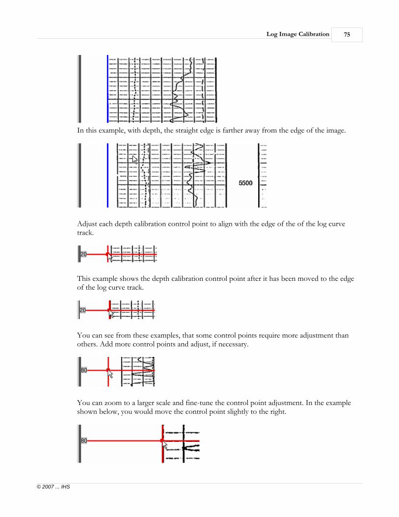
Log Image Calibration 75
© 2007 ... IHS
In this example, with depth, the straight edge is farther away from the edge of the image.
Adjust each depth calibration control point to align with the edge of the of the log curvetrack.
This example shows the depth calibration control point after it has been moved to the edgeof the log curve track.
You can see from these examples, that some control points require more adjustment thanothers. Add more control points and adjust, if necessary.
You can zoom to a larger scale and fine-tune the control point adjustment. In the exampleshown below, you would move the control point slightly to the right.

Getting Started76
© 2007 ... IHS
Click on the "EditàStraighten Image Edges…" menu option or the "Straighten Image" icon
.
After, clicking on the "OK" button on the "Confirm" dialog screen, when you scroll downthe image, you will see that the image has been straightened.
The message shown below will be displayed during the straightening of the image.
You will see an "Information" message displayed telling you that the image has beenmodified with a reminder to save the image to a new file name. Click on the "OK" button tocontinue.
Click on the "FileàSave Image As…" menu to save the image to a new name.
A "Save Image as TIF File" dialog screen will be displayed
Enter the new file name for the image. For our example, we will use "D-122_Straightened.tif" as the file name. After entering the name for the straightened image,click on the "Save" button.
The dummy calibrations used for straightening the image need to be cleared out of memory.Click on the "EditàClear All Calibrations..." menu.
The following confirmation dialog screen is displayed. Click on the "Yes" button. Thedummy calibrations will be cleared from memory. You are now ready to calibrate the image.

Log Image Calibration 77
© 2007 ... IHS
5.2 Depth Calibration - Log Image
If you are not in the "Calibrate Log Image" module, from the cross section you can bringup the calibration module by clicking on the "RasterLogsàLog Image Calibration…"menu
Optionally, you may right click on the well that you want to assign the image to and clickon the "Calibrate Log Image…" option.
From the "Main" module, you can bring up the calibration module by clicking on thewell, in our case, WSN 21, then on the "Raster" tab and then on the "Assign/Calibrate"button.
Once you get to the "Calibrate Log Image" dialog screen, either from the "Main" moduleor from the "Cross Section" module, the calibration procedure is the same. When the"Calibrate Log Image" dialog screen is displayed you will see a series of drop downmenus across the top, the "DEFAULT" image group name, and the well that has beenselected prior to coming into the "Calibrate Log Image" dialog screen.
We will load the image into the "Calibrate Log Image" dialog screen by clicking on the"FileàOpen Image…" menu.
Click on the D-122.tif image and click on the "Open" button. After the image is loaded,click on the "Zoom - +" buttons, as needed to see a reasonable amount of the image.
5.3 Image Groups
The cross-section displays log images for a given well by referencing group names. Forexample, you might display images from the "GR" group in track 1 and images from the"Default" group in track 2.
PETRA predefines one group called the "Default" group. An image can be calibratedusing this group name, however it cannot be deleted or replaced. You can create as manyadditional groups as you have log types in a project. Groups names should normally havesomething to do with either the log curves they contain or the sample rate (number ofinches per 100 feet) of the log, i.e., "5-inch logs".

Getting Started78
© 2007 ... IHS
Each well can have only one image or vertical slice of an image in a group. However,there is no limit to the number of different groups you can define. Therefore, if you have5 different log images for a well, you must have 5 different image groups defined. Thewell will have 1 image in each of the 5 groups.
The PETRA database has a table containing a reference to log image calibrations. Eachrecord in the table contains a well sequence number (WSN), image group number (IGN)and a path to the calibration file. This scheme allows an unlimited number of images tobe referenced for any given well.
To add a new group click on the "Group" menu item, the "Add or Delete Groups…"menu option will be displayed. When you click on this option a "Log Image GroupMaintenance" dialog screen is displayed.
Enter a new "Group" name in the "Image Group Name (Case Sensitive) data field andenter a description for the new group in the "Image Group Description" data field. Click
on the "Add" button with the blue plus to add the new group to the "LogImage Groups" section.
Another way to add a new group is to click on the small "+" button to the right of"Group" at the top of the calibration screen. A "New Image Group Name" dialog screenin is displayed with a "Enter New Group Name" data field. Enter the new "Group" nameand click on the "OK" button. You will see the new group name when you click on the
"Drop Down" selection button to the right of the "Group" data display field.
The log images for different log types can be saved as a different group. For instance, youmight want to call the 5 inch gamma ray GR_5IN. Other examples are:NeutronDensity_2_5IN, Resistivity_1IN, Elog, etcetera.
5.4 Calibrating A Log Image
The "Depths" Calibration Menu has the following options:
· Image Depth Type - Remember to set the type to TVD for TVD images. Thedefault is MD.
· Image Depth Units Are· Display Depths As· Go To Depth... ("Ctrl+G" function keys)· Go to First Calibrated Depth· Go to Last Calibrated Depth· Restore Original Depths...· Adding Depth Point· Delete Depth· Delete All Depths...· Interpolate Depths...· Set Est. Depth Rounding Factor...

Log Image Calibration 79
© 2007 ... IHS
· Set Depth Pick Tolerance· Set Depth Shift Amount...
5.5 The Image Calibration Tool Bar
The "Depth Calibration" tool bar is located on the right hand side of the "Calibration"dialog screen and has several parts to it.
The "Go To Top Depth" and "Go To Bottom Depth" buttons are at the top ofthe tool bar. When you click on the "T" button, the image will be displayed at the firstcalibration depth. When you click on the "B" button, the image will be displayed at thelast calibration depth.
The "Previous Depth" button, function key "F7", and "Next Depth" button, functionkey "F8" buttons are next. When you click on the "Previous Depth" button orthe function key "F7", the image will be displayed at the previous calibration depth.When you click on the "Next Depth" button or the function key "F8", the image willbe displayed at the next calibration depth.
The "Depths" section is next and contains the "Add", "Drop", "Interp..." and Dec..."buttons.
When you click on the "Add" depth button , a horizontal blue line is displayedwhen the cursor is placed on the image. You will move the blue line to a depth on theimage and left click to anchor the line at that depth. A "Depth Calibration" dialog screenwill be displayed. Enter the depth value the blue line represents and click the "OK"button. The line will turn red and the depth entered will be displayed on the image.

Getting Started80
© 2007 ... IHS
When you click on the "Drop" button , you will move the cursor to a calibrationdepth line to select it. When it is selected and you left click on the calibration line, thecalibration depth will be deleted.
The "Interpolation" button is used to interpolate depths between the uppermostand lowermost depths. You will enter the interpolation increment.
The "Decimate Depths" button is used to decimate the calibration depths. Whenyou click on this option, a "Confirm" dialog screen is displayed. If you want to proceed,click on the "OK" button.
Enter a number for the decimation and click the "OK" button.
The results of the decimation will be displayed. Click on the "OK" button to completethe transaction. Remember to save your calibration file.
The "Edges" section is next and contains the "Left" and "Right" buttons.
When you click on the "Left" edge button , a vertical blue line is displayed whenthe cursor is placed on the image. You will move the blue line to the left edge of theimage and left click to anchor the line at that edge. The line will change to a thin blue linewith an indicator pointing to the right of the image.
When you click on the "Right" edge button , a vertical blue line is displayed whenthe cursor is placed on the image. You will move the blue line to the right edge of the

Log Image Calibration 81
© 2007 ... IHS
image and left click to anchor the line at that edge. The line will change to a thin blue linewith an indicator pointing to the left of the image.
The "Header" section is next and contains the "Top" and "Bottom" buttons.
When you click on the "Top" header button , a horizontal blue line is displayedwhen the cursor is placed on the image. You will move the blue line to the top of the"header" on the image and left click to anchor the line at that point. The line will turngreen and the keyword "HDRTOP" will be displayed to the right of the image.
When you click on the "Bottom" header button , a horizontal blue line isdisplayed when the cursor is placed on the image. You will move the blue line to thebottom of the "header" on the image and left click to anchor the line at that point. Theline will turn green and the keyword "HDRBOT" will be displayed to the right of theimage.
The "Footer" section is next and contains the "Top" and "Bottom" buttons.
When you click on the "Top" footer button , a horizontal blue line is displayedwhen the cursor is placed on the image. You will move the blue line to the top of the"footer" on the image and left click to anchor the line at that point. The line will turngreen and the keyword "FTRTOP" will be displayed to the right of the image.
When you click on the "Bottom" footer button , a horizontal blue line is displayedwhen the cursor is placed on the image. You will move the blue line to the bottom of the"footer" on the image and left click to anchor the line at that point. The line will turngreen and the keyword "FTRBOT" will be displayed to the right of the image. Since thisimage does not have a footer, the display shows the same section of the image as the"Header".

Getting Started82
© 2007 ... IHS
The last section is the "Contrast" control slider. You will move the slider bar up to darkenthe image and down to lighten the image.
5.6 Assign A Group Name
Select the appropriate image group from the "Image Group Name" drop-down list orAdd a new group using the "GroupàAdd or Delete Groups..." menu. Refer to the Imagegroups section above for more detailed information. For our purposes, we will use theDefault group.
5.7 Define the Calibration Depths
This process involves picking 2 or more depths from the image. Each depth point ispicked by first choosing the "EditàAdd Depth Point" menu or by clicking the "Add"
button located at the top of the Calibration Tool Bar. Position the horizontalcursor exactly at the depth you wish to pick, then click the left mouse button. You will beprompted for the depth value. After entering the depth value, the screen will redrawshowing you the new calibration depth point. Repeat the process for each depthreference point. When all of the depths have been entered, you can click with the right
mouse button, or click on the "Add" button to get out of the "Add Depth Point"mode. Position the horizontal blue line at the top depth line and click the left mousebutton.
A "Depth Calibration" dialog screen will be displayed. Enter the depth that the blue linewas dropped on. In our case it is 7746 and click the "OK" button.
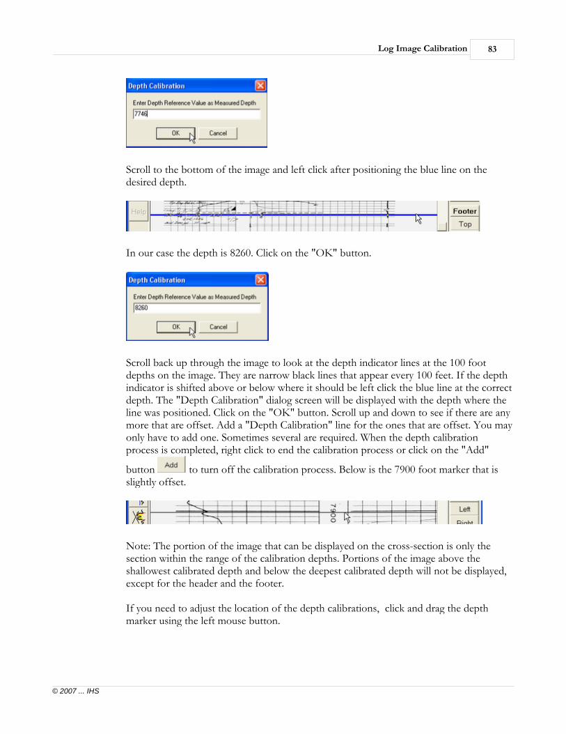
Log Image Calibration 83
© 2007 ... IHS
Scroll to the bottom of the image and left click after positioning the blue line on thedesired depth.
In our case the depth is 8260. Click on the "OK" button.
Scroll back up through the image to look at the depth indicator lines at the 100 footdepths on the image. They are narrow black lines that appear every 100 feet. If the depthindicator is shifted above or below where it should be left click the blue line at the correctdepth. The "Depth Calibration" dialog screen will be displayed with the depth where theline was positioned. Click on the "OK" button. Scroll up and down to see if there are anymore that are offset. Add a "Depth Calibration" line for the ones that are offset. You mayonly have to add one. Sometimes several are required. When the depth calibrationprocess is completed, right click to end the calibration process or click on the "Add"
button to turn off the calibration process. Below is the 7900 foot marker that isslightly offset.
Note: The portion of the image that can be displayed on the cross-section is only thesection within the range of the calibration depths. Portions of the image above theshallowest calibrated depth and below the deepest calibrated depth will not be displayed,except for the header and the footer.
If you need to adjust the location of the depth calibrations, click and drag the depthmarker using the left mouse button.

Getting Started84
© 2007 ... IHS
5.8 Define the Left and Right Edges of the Image
Set the leftmost edges of the image to display by using the "EditàSet Left-Most Edge"
menu or by clicking the "Left" button under the "Edges" portion of the "ImageCalibration" tool bar. Position the vertical cursor at the leftmost point of the image totrim the left edge. Set the rightmost edges of the image to display by using the "EditàSet
Right-Most Edge" menu or by clicking on the "Right" button under the "Edges"portion of the "Image Calibration" tool bar. Position the vertical cursor at the rightmostpoint of the image to trim the right edge. Shown is an example of the left and right edgeswith the edge indicator pointing in from each edge.
Note: To adjust the location of either edge marker, click and drag the marker using theleft mouse button.
5.9 Define the Log Header Section
Click on the "EditàHeadersàSet Header Top" menu or click on the "Top" header
button , a horizontal blue line is displayed when the cursor is placed on the image.You will move the blue line to the top of the "header" on the image and left click toanchor the line at that point. The line will turn green and the keyword "HDRTOP" willbe displayed to the right of the image. The header section normally is the area of theimage containing the log track scales.
Next click on the "EditàHeadersàSet Header Bottom" menu or click on the "Bottom"
header button , a horizontal blue line is displayed when the cursor is placed on theimage. You will move the blue line to the bottom of the "header" on the image and leftclick to anchor the line at that point. The line will turn green and the keyword"HDRBOT" will be displayed to the right of the image.
To change the location of either header marker, click and drag the marker using the leftmouse button

Log Image Calibration 85
© 2007 ... IHS
5.10 Define the Log Footer Section
For this example, we will use the "Header" portion of the image as the "Footer" sincethere is not a separate header and footer for this image.
Click on the "EditàFootersàSet Footer Top" menu or click on the "Top" footer
button , a horizontal blue line is displayed when the cursor is placed on the image.You will move the blue line to the top of the "footer" on the image and left click toanchor the line at that point. The line will turn green and the keyword "FTRTOP" will bedisplayed to the right of the image. The header section normally is the area of the imagecontaining the log track scales.Next click on the ""EditàFootersàSet Footer Bottom"" menu or click on the
"Bottom" footer button , a horizontal blue line is displayed when the cursor isplaced on the image. You will move the blue line to the bottom of the "footer" on theimage and left click to anchor the line at that point. The line will turn green and thekeyword "FTRBOT" will be displayed to the right of the image.

Getting Started86
© 2007 ... IHS
To change the location of either footer marker, click and drag the marker using the leftmouse button.
5.11 Deleting Calibration Depths
Individual depth references can be deleted using the "DepthsàDelete Depth" menu orclicking the "Drop" button located in the "Depths" section of the "Calibration" tool bar.After invoking the delete function, click the left mouse button on the depth marker to bedeleted. The screen will redraw once the marker is deleted.
You can also delete all depth references using the Menu Option "DepthàDelete AllDepths...".
5.12 Saving the Calibration File
Choose the "FileàSave Calibration As..." menu to save a file containing the calibrationdata, image name, depth references, etcetera. This will also update the PETRA databasewith a reference to the calibration file, which is now associated with the current well.
Log Image Calibration files have a file extension of ".LIC.
Click on the "Save File" button with the green check to save to the defaultfile name. You can change the name to another name. It is suggested that you keep theUWI/API as part of the file name.
Click on the "OK" button to confirm the information associated with the calibration file.
Click on the "OK" button.
To end the calibration session, click on the "FileàExit" menu or click on the red "X" inthe upper right of the dialog screen.
5.13 Loading a Calibration File
You can load and modify a previously saved calibration file using two methods.
First, the "FileàLoad Calibration File..." menu allows you to choose the specificcalibration file to be loaded. The image name will be read from the calibration file and theimage will be opened and displayed.
Secondly, the "FileàLoad Calibration For Group..." menu will retrieve the name of thecalibration file from the PETRA database which is associated with the current well andimage group name.

Mapping Module 87
© 2007 ... IHS
6 Mapping Module
The mapping module provides essential display functions for any project.
In the Main Module, click on the icon or the "ToolsàMapping" menu to display the mapmodule.
6.1 Mapping Module Overview
The mapping module is initiated using the "ToolsàMapping" menu option on the Main screen
or the "Mapping" icon .
When the map opens, it will retrieve certain information about each well. A "Loading Wells" fuelgauge will show the progress while the map is initialized. Once initialized, the well symbols willappear on a white background. Note the map scale in the lower left corner of the mappingwindow as well as the number of wells that are displayed on the map.
The wells are shown with the WellsàDirectional SurveyàEnabeled option turned on. The wellsymbols will not be labeled initially. We can add annotations around the well symbol using the
"OptionsàData Posting" menu or the "Post Well Data" icon to display the "Data Posted

Getting Started88
© 2007 ... IHS
By Well Spot" dialog screen. Under the "Available Data Items" options, there is a "Well Header
Items" "Drop Down List" button. After clicking on the "Drop Down List" button , click on
the "API Series No." data item and click on the "Move Selected Item" button to move thedata item to the "Selected Data Items" list box. Under the "Data Item Details" menu, change the"Position" to "Above".
Note that there is a "Posting Sample" display, in the upper left portion of your screen. Thisshows how the data would look on the map after it is posted.
Click the "OK" button. The map is redrawn with well labels plotted above each well.
Note: You can move the "Data Posted By Well Spot" dialog screen to the right, if it is on top ofthe "Posting Sample" window. This will allow you to see the "Posting Sample" window, whichwill show you how the well will be annotated. This window is displayed in the upper left portionof your screen.
"Quick List" feature
The option "Display>Preferences (Margins, North Arrow, etc)..." has a setting that was turnedon for this display.On the "General" tab, under "Data Extents" the "Extend Data To Border Frame" has been set.
The "Quick List" feature consists of 3 list boxes down the left side of the map window. Theupper list provides quick access to map data items like posted text, contours, attribute and bubblemap templates. The middle list displays all overlay layers containing data. The lower list allowsyou to select multiple wsn lists to control the wells on the map. The quick lists are made visible
using the small icon located to the left of the Print icon. An "auto refresh" option at thebottom of the quick list panel allows immediate map refresh when a list check box is toggled.When not in auto mode, you must click a small "apply" button at the top of the lists.
In the "Map Data" list, you will double click on a item to bring up the associated dialog screenfor selecting or changing the parameters that are needed for the map. To turn the item off, clickthe check box to the left of the item. If the item is not grayed out, you can turn the item on byclicking the check box to the left of the item. If the item is grayed out, double click on the itemto set the parameters for the item.

Mapping Module 89
© 2007 ... IHS
6.2 Land Grid Overlay
Political and cultural data are available from commercial data suppliers such as: Whitestar, TobinData Graphics, or some other commercial vendor. The data is also available from the WEB atvarious locations. PETRA can import these data using the map "Overlay" utility. This tutorialcontains a sample of a land grid that has been imported from the original vendor's format andsaved as a binary "Overlay" file. You can load and display the land grid by choosing the"OverlayàLoadàOverlay File" and selecting the file named "LANDGRID.OVL". The mapoverlay will be discussed in more detail later in this tutorial.
To show all of the cartographic data that was loaded into the overlay, click on "DisplayàDataLimitsàUse Overlay Extents".
6.3 Selecting a Well On the Map
When you single click a well symbol with the left mouse button, the well is highlighted to indicateselection. Several editing options are available for a selected well, including, moving the location,dropping from the map, or deletion from the project.
When you double click on a well symbol with the left mouse button, PETRA will immediatelyjump to the "Main" module screen positioned at the selected well if that well is one of the wellsthat are selected in the "Main" module. This feature can be used to quickly access any data for aspecific well. To return to the map, either click on the "Map - PETRA" task on the Windows task

Getting Started90
© 2007 ... IHS
bar or click the "Mapping" icon . Shown below is the task bar from XP.
To return to the "Map" with the cursor pointing to the selected well, click on the "Highlight Well
On Map" icon or use the "F8" function key.
6.4 Viewing Data For a Specific Well
Well information is displayed whenever you click the right mouse button on a well symbol.
A pop up menu shows the basic well header data, with an option to select items to be displayedfor the selected well and to change the symbol size for that well.
When you select the "Layers..." option, the "Overlay Layers" dialog screen will be displayed asshown below.

Mapping Module 91
© 2007 ... IHS
When you select the "Active/Inactive Options..." option, you will see the "Disable and EnableMap Options" dialog screen. Place a "check" by the options that you want to display. If there isan option that you want to disable, click the check box to the left of the option(s) that you wantto disable.
When you click on the "User FavoritesàSelect…" option a dialog screen will be displayed whereyou can select additional items that you would like to see displayed when you use the "RightClick on a Well" option.

Getting Started92
© 2007 ... IHS
Click on either the "Well Header Data" drop down list button or on the "Zone Data Item"
drop down list button . A list of items will be displayed, from which you can select the itemsthat you would like to see displayed when you right click on a well and click on the "User
FavoritesàSelect…" option. Click on the "Add" button to add the item to the"Selected Data Items" selection list. Click on the "OK" button to close the "Well Data Selection"dialog screen. Right click on a well and click on the "User FavoritesàSelect" option. You will seeyour favorites displayed in the drop down display screen.
The selected favorites are shown in the right hand display. To change the "User Favorites", clickon the "Select…" menu item and add or remove the items that you want to see displayed.
6.5 Finding A Specific Well
To locate a specific well on the map, first go to the "Main" module and select the desired well in
the well list. Then, click the "Highlight Well On Map" icon or use the "F8" function key.The system will jump to the map with the selected well highlighted. The mouse cursor will pointto the highlighted well.

Mapping Module 93
© 2007 ... IHS
Note: This feature only works when the mapping module is open.
6.6 Zooming
You can enlarge a portion of the map by setting a "zoom" rectangle. Select the "DisplayàZoom
In" menu or click the "Zoom In" icon. The cursor will change to a magnifying glass.Position the cursor at the upper left corner of the region to be enlarged. Click and hold down theleft mouse button while dragging the lower right corner of the rectangle so that it encloses theregion to enlarge. Release the left mouse button. The map will redraw showing that portion ofthe map falling inside the zoom window. Note the change in map scale. You can repeat the
process to further zoom in. Use the "DisplayàZoom Out" menu or icon to revert to the
previous zoom window. The "DisplayàZoom Off" or "Turn Zoom Off" icon sets the mapback to the original limits.
6.7 Panning and Scrolling
Once in the zoom mode, the screen can be scrolled up, down, left or right by pressing one of thearrow keys while holding down the shift key. The screen can also be panned in any direction by
clicking the "Pan" icon and clicking and dragging with the left mouse button to the newposition. The screen will be re-drawn with the map positioned at the new location.
If you prefer to use the keyboard to navigate, here are the function keys that can be used:
Menu Function KeysDisplayàZoom In Ctrl+ZWhile Zoomed in, press the "+" "-" keys to zoom in and out by ¼ of the zoomed extentsDisplayàZoom Off Alt+ZDisplayàPan F10
6.8 Posted Base Maps
Base maps typically show various information posted around each well symbol. Data posting
options are available using the "OptionsàData Posting" menu or the "Post Well Data" icon. Up to 50 data lines can be posted. Each item can be located in one of 4 blocks: above,below, left or right of the well spot. The text height and color can be set for each line item. Textsizes can be specified in inches or Map X/Y's.
6.9 Selecting and Formatting Posted Data
Select the "OptionsàData Posting" menu or click on the icon to display the "Data PostingBy Well Spot" dialog screen.
Notice the "Available Data Items" section in the upper left portion of the dialog box. Posted dataitems are chosen from this section and added to the "Selected Data Items" list on the right by

Getting Started94
© 2007 ... IHS
clicking the associated "Add Well Header Items" button . For example, select the "API Series
No" from the "Well Header Items" group and click the "Add Well Header Items" button justto its right. A line reading "API Series No." is added to the "Selected Data Items" list. You canchange the color by clicking the color below the "Text Color" option. A "Color" palette will bedisplayed. Click on the "color" that you would like to assign to the text and click on the "OK"
button . Set the "Position" to "Above". Set the "Text Height" to read 0.1. Click on the
"Options" tab, and click on the drop down button to the right of "All Sizes Are In" to select"inches".
Next, we will add a line item below the well showing the total depth of the well. In the "AvailableData Items" section, locate and select the "Zone Data Items" zone called "WELL" and the item
called "TD". Click the "Add Zone Item" button next to the zone drop down list. The phrase"WELL - TD" is added to the "Selected Data Items" list. Set the position to "Below" and the textcolor to black. Try adding other data items noting the change in the "Posting Sample" window.Click the "OK" button to return and redraw the map.
Try zooming in to reduce clutter. Once again, invoke the Data Posting option. Click on the"Options" tab and click the box beside the "Enlarge with Zoom" option. Click the "OK" buttonto redraw the map. Now when you zoom in, the posted data text will enlarge somewhat makingthe text easier to read.
To turn off or disable data posting, invoke the Data Posting option once more. Click the checkbox beside the "Active" option so that it is in the unchecked state. Click the "OK" button toreturn and redraw the map without any well annotation. The posting options will be retained andcan be reactivated by simply invoking the posting option and clicking the "OK" button.
Note: Data posting can also be disabled and/or reactivated from the"OptionsàActive/Inactive" menu or from the "Quick List" menu which can be displayed on theleft side of the map..
The "Options Tab" has several check boxes that can be set. There are some options that cancontrol the distance between the well and data; the line spacing for the text, a global scale factor,and a drop down list to set the sizes in inches or map XY's.
The "Wells Tab" has some additional options that can be set. You can post data for all wellsdisplayed on the map, which is the default, highlighted wells only, or wells that you have selectedin a Well Sequence Number (WSN) List.
The "PdCum Tab" has options for posting the PdCum data.
The "Misc Tab" has options for "Zone Items Legend" data, Legend Text Size MultiplicationFactor, and a Wrap Zone Text Items to a specified number of characters. The default is to notwrap the text data.
The "Overposting Tab" has options for the "Manually Shifted" text as well as "Automatic

Mapping Module 95
© 2007 ... IHS
Overpost Resolution". There are check boxes to "Hide Connecting Line" and "Draw TopConnecting Line".
If you have moved text, there is a button to clear shifted text for all wells, labeled "Clear DBShifted Text...".
6.10 Contour Maps
Contour maps are generated by constructing gridded surfaces from wells, faults, overlaycontours, user control points, and/or seismic z values. A grid file contains regularly spaced valuesinterpolated from the original data. Contours are drawn from the gridded surface data. PETRAprovides an easy to use interface for choosing gridding and contouring options.
Grid files cannot be displayed for a projection that is different than the one it was created with.The file contains X/Y values that are based on the projection the "Map" is in when the grid iscreated.
6.10.1 Creating a Structure Map Grid
To illustrate the gridding and contouring process, we will create a structure contour map of the"A" formation top.
Note: The following step is only required for projects containing directional wells. Before goingthrough this step, you might want to read the next "Note" below.
The well locations currently displayed are based on the maximum directional survey depths.Before we grid the data it is important to set the well locations to the projected location of "A"formation.
Use the "WellsàDirectional SurveyàSet Location Depth" menu to display the "DirectionalWell Location Definition" dialog screen.
When the "Directional Well Location Definition" dialog screen is displayed, click on the "Drop
Down" selection button and select the "Locate Wells at Formation Top Depth" option.
Click on the "Depth Parameters Fm Top" drop down list button and select the "A"Formation.
Click the "OK" button with the green check.The new well locations will be recomputed. We are now ready to create the "A" formation grid.
Begin by choosing the "ContoursàCreate Grid" menu option
or the "Create a Grid" icon . The "Create Contour Grid" screen is displayed.
Note: You can also use an option on the "Create Contour Grid" dialog screen to set the proper"XY" for the formation that is to be contoured by checking the "Check" box to the left of "Cal

Getting Started96
© 2007 ... IHS
XY For Dev Wells At Top:". The drop down list button can be used to select the desired top.
From the "Data" tab section, locate and select the "FMTOPS" zone name and the "A" formationtop name. Note how the grid title and file name fields adjust automatically. You can change thesefields if you wish or use the defaults. There should be a check mark by the box that reads "ZoneData". Also, place a check mark by the box labeled, "Use TVD Subsea Tops" so that we get astructure map and not a map of the measured depths.
Click on the "Method" tab. Click on the "Estimate Grid Size From Z Data" radio button.
Click the "OK" button with the green check to initiate the gridding task.
Note: You may want to experiment by increasing or decreasing the grid size or using differentsurface style options.
Computing the grid for this small project won't take long. However, to accommodate largerprojects, gridding is performed as a background job so you can continue doing other thingsduring longer gridding tasks. This sample gridding screen was captured from an example withmuch more data. More than one gridding task can be active simultaneously. Once the griddingtask completes, we are ready to display our contour map.
6.10.2 Structure Map Contouring
PETRA simplifies the contouring process and produces a reasonable map on the first try bycomputing default values for contour range and interval using grid file statistics. Most of the timeyou simply select a grid file and click OK to see the contours. However, there are several optionsfor controlling contour range, interval, color scheme, and labeling style.
Invoke the contouring option by selecting the "ContoursàDisplay Contours..." menu item
or by clicking the "Contour a Grid" icon. The "Contour a Grid" screen will appear with thefile "FMTOPSA.GRD" pre-selected. By default, Grids are listed in descending date order. Tosort the grid files by name, click on the radio button to the left of "By Name".
Note that PETRA has already computed the contour range and interval.
Click on the "Options" Tab to look at the available options. We will use the seven options thatare checked at this time.
Click the "OK" button with the green check to display the contour map.
Select the "ContoursàDisplay Contours..." menu item

Mapping Module 97
© 2007 ... IHS
or "Contour a Grid" icon again. This time, click the "Options" Tab and click the "ColorFilled Contours" option so that it is "checked". Click on the "Draw Color Bar Scale" option todisplay the color bar. Click the "OK" button to see a color filled contour map with the color bardisplayed on the map.
6.10.3 Contour Range and Color Palette
Again select the "ContoursàDisplay Contours..." menu item
or "Contour a Grid" icon. This time, click the "Colors" button on the "Grid" Tab screen.PETRA displays the "Color Interval Definition" screen to select the color for each contourinterval. The current color intervals are displayed in the center list. To change an interval color,click once on its row in the interval list. Notice how the color palette indicates the current color.Next, click once on a color palette cell to change the interval to a new color. Click the "Help"button for many more features such as changing the number of color intervals, editing the colorpalette, and blending colors using interpolation.
Click the "OK" button with the green check to close this dialog screen. The changesthat you have made will be kept.
6.10.4 Contouring With Faults
PETRA provides a very easy method to incorporate fault discontinuities into gridded surfaces.Faults can be added to a map using the "Overlay" feature, which is discussed in more detail in the"Map Overlay Utility" chapter. Read the "Adding an Overlay Line" "Editing Line Attributes"paragraph. In general, faults can be "digitized" from the screen as a series of points tracing thefault line or polygon. You then turn on the "Include Faults" option when the grid is created.
6.10.5 Creating An Isopach
PETRA offers three methods for generating isopach contour maps. The first example showshow to grid and contour the computed interval thickness at each well, the second, illustratesgridding the upper and lower structures of our formation, then computing and contouring thedifference between these surfaces, the third method uses the grid to grid calculation method.
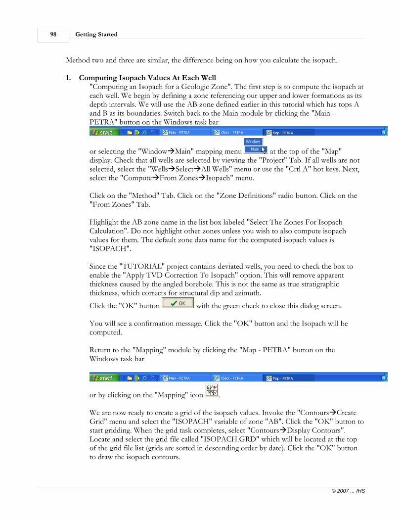
Getting Started98
© 2007 ... IHS
Method two and three are similar, the difference being on how you calculate the isopach.
1. Computing Isopach Values At Each Well"Computing an Isopach for a Geologic Zone". The first step is to compute the isopach ateach well. We begin by defining a zone referencing our upper and lower formations as itsdepth intervals. We will use the AB zone defined earlier in this tutorial which has tops Aand B as its boundaries. Switch back to the Main module by clicking the "Main -PETRA" button on the Windows task bar
or selecting the "WindowàMain" mapping menu at the top of the "Map"display. Check that all wells are selected by viewing the "Project" Tab. If all wells are notselected, select the "WellsàSelectàAll Wells" menu or use the "Crtl A" hot keys. Next,select the "ComputeàFrom ZonesàIsopach" menu.
Click on the "Method" Tab. Click on the "Zone Definitions" radio button. Click on the"From Zones" Tab.
Highlight the AB zone name in the list box labeled "Select The Zones For IsopachCalculation". Do not highlight other zones unless you wish to also compute isopachvalues for them. The default zone data name for the computed isopach values is"ISOPACH".
Since the "TUTORIAL" project contains deviated wells, you need to check the box toenable the "Apply TVD Correction To Isopach" option. This will remove apparentthickness caused by the angled borehole. This is not the same as true stratigraphicthickness, which corrects for structural dip and azimuth.
Click the "OK" button with the green check to close this dialog screen.
You will see a confirmation message. Click the "OK" button and the Isopach will becomputed.
Return to the "Mapping" module by clicking the "Map - PETRA" button on theWindows task bar
or by clicking on the "Mapping" icon .
We are now ready to create a grid of the isopach values. Invoke the "ContoursàCreateGrid" menu and select the "ISOPACH" variable of zone "AB". Click the "OK" button tostart gridding. When the grid task completes, select "ContoursàDisplay Contours".Locate and select the grid file called "ISOPACH.GRD" which will be located at the topof the grid file list (grids are sorted in descending order by date). Click the "OK" buttonto draw the isopach contours.

Mapping Module 99
© 2007 ... IHS
2. Isopach Map From Structure Grids
The second method for constructing an isopach map of the "AB" interval involvescreating two structure grids, one for formation "A" and one for formation "B". We thensubtract grid "B" from grid "A" to create a third grid, which contains the isopach values.Begin by creating a grid of the formation "B" top following the same procedure used tocreate the structure grid for "A". Don't forget to set the well symbol location depth to the"B" formation, using the "WellsàDirectional SurveyàSet Location Depth" menu. Afterthe "B" grid is generated, select the "ContoursàGridsàIsopach and TST..." menu. Thisoption performs mathematical operations between two grids.
Using the drop down list button in the "Upper Surface Grid" section to find andselect the "FMTOPSA.GRD" file name.
Using the drop down list button in the "Lower Surface Grid" section to find andselect the "FMTOPSB.GRD" file name.Enter the name, "AB.GRD" in the "Output Isopach Grid" or use the drop down list box
to select an existing grid file that you want to overwrite. Enter a grid title, such as,"Isopach using A and B Grids".
Click on the "Compute" button with the green check to compute theisopach.
There is no correlation intended in naming the sample tops (A and B) and the two inputgrids (A and B).
This following message box will be displayed confirming the Grid to Grid Option thatwas chosen and the grids that are to be used for A and B. The Output grid is shown aswell. If the output grid file already exists, you will get a message asking if you want toreplace the existing grid file. Click on the "Yes" button if you want to replace the file.
A warning message will be displayed if the number of rows and columns are not the samefor both grid files
When this warning is displayed, you will use the "ContoursàGridsàResample Grids ToMatch…" menu option to resample the grid with the smallest number of rows andcolumns to the grid with the largest number of rows and columns.
Click on the drop down list button to the right of the "Grid To Match All ResampledGrids (Source) data field to select a grid file.
Click on the "Grid Info..." button to display the information for that file.Change the grid file to the FMTOPSA.GRD file to check the information for that file.
Click on the "Close" button with the green check to close the "Grid

Getting Started100
© 2007 ... IHS
Information" dialog screen.
Change the grid file to the FMTOPSA.GRD file to check the information for that file.
You want to select the grid file with the largest number of rows and columns as the "GridTo Match All Resampled Grids (Source)" grid file. The FMTOPSB.GRD file has themost rows and columns. That file will be used as the source file.
For the "Grids To Resample (Target)" file selection, you will select the grid(s) that youwant to match the source grid by clicking on the grid file name(s). In our case, you willselect the FMTOPSA.GRD, since we have selected the FMTOPSB.GRD as the sourcefile. After the source and target grid files have been selected click on the "OK"
button with the green check.
A "Resample Grid(s)" information screen will be displayed. Click on the "OK" button. The resampled grids will be renamed to "RS_gridfilename".
A RS_FMTOPSA.GRD file will be created. Use that file to compute the AB GridIsopach.
After completing the steps necessary to create the output grid that contains theISOPACH using the Grid To Grid operation, display the resulting grid file, "AB.GRD"using the "ContoursàDisplay Contours" option.
3. Isopach Map From Structure Grids using the Grid To Grid Calculations Method
The third method for constructing an isopach map of the "AB" interval involves creatingtwo structure grids, one for formation "A" and one for formation "B". We then subtractgrid "B" from grid "A" to create a third grid, which contains the isopach values. Begin bycreating a grid of formation "B" top following the same procedure used to create thestructure grid for "A". Don't forget to set the well symbol location depth to the "B"formation, using the "WellsàDirectional SurveyàSet Location Depth" menu. After the"B" grid is generated, select the "ContoursàGridsàGrid-To-Grid Calculations" menu.This option performs mathematical operations between two grids.
Enter the name, "AB.GRD" in the "C" drop down list box in the "Output Grid File"section. Enter a grid title, such as, "Isopach using A and B Grids". Next, locate and selectthe "Grid Operation" entitled, "C=A-B". For the Input Grids section, select the"FMTOPSA.GRD" for the "A" Input grid file and "FMTOPSB.GRD" as the "B" inputgrid file. Click the "OK" button to start the calculation.
There is no correlation intended in naming the sample tops (A and B) and the two inputgrids (A and B).
Confirm message box will be displayed confirming the Grid to Grid Option that waschosen and the grids that are to be used for A and B. The Output grid is shown as well.

Mapping Module 101
© 2007 ... IHS
You could possibly see the same warning message about the grids stating that they musthave the same number of rows and columns as described above. You will follow thesame procedure as mentioned above to resample the grids to match.
6.11 Bubble Maps
Bubble maps display one or more z data variables as a color-filled circle or circle segment at eachwell. The radius of each circle can vary in size depending on the z value magnitude, or can be aconstant size for all wells. Bubble maps are ideal for displaying highly variable data such ascumulative oil and gas production. Bubble maps can also provide a good quality control tool toquickly show which wells have good values. For example, while correlating formation tops fromcross sections, you might display the top you are picking as a fixed radius bubble map. You caneasily keep track of which wells have not been picked and which cross sections need to bedisplayed.
If the contours from the previous example are still being displayed, click on the
"ContoursàHide Contours" menu or the "Hide Contours" icon to turn the contours off.
You can also, click on the "Check" box to the left of "Contours" in the "Quick List" to turn offthe contour display.
For this tutorial we will display the cumulative gas production we computed during thediscussion on Main's "Production" tab. The values are stored in the "WELL" zone as a itemname called "CUMGAS". Invoke the "Bubble Map Options" screen by selecting the Map's
"OptionsàBubble Map" menu or by clicking the "Bubble Map" icon.
The "Bubble Map Options" screen is divided into two sections. The "Data Items For Bubbles(Max 32)" list shows the item names currently selected for the bubble map. Each bubble can becomposed of up to 32 segments from 32 different Z data items. The right half of the screenconsists of several tabbed sections used for data selection and parameter settings. Our cumulativegas production bubble map begins by locating and selecting the "CUMGAS" item of the"WELL" zone from the two drop down list boxes within the "Select Z Data Used For Bubbles"section on the "Z Data" tab screen. First, change the upper list box to the "WELL" zone. Thelower list box will show all "WELL" zone data items. Locate and select the "CUMGAS" dataitem. Notice how the "Value Range" section adjusts to give appropriate default values. Click the"Colors" button to change the color scale and palette using the same technique described under
contouring. Click the "ADD" button with the blue "+" to add the "CUMGAS" data item tothe selection list.
Click on the "Radius" tab and choose the "Vary Radius as Units/Inch" option by clicking the"Radio" button to the left of this option. Type a radius/inch value of 20000000.
And finally, click the "OK" button to draw the bubble map.

Getting Started102
© 2007 ... IHS
6.12 Map Overlay Utility
The map overlay utility provides the capability to create, import, edit and display political andcultural data such as land grids and lease outlines. In general, the overlay utility allows arbitrarylines, text, and polygons to be added to maps. The overlay is composed of 256 user definablelayers. Each layer can be displayed and manipulated independently. A layer contains one or moregraphical element types. There are two basic graphical element types: lines and text.
The overlay utility also allows PETRA users to define geologic faults used for contour mapconstruction. Contour maps can be "captured" to an overlay layer where contours can bemodified and re-entered as control points to the gridding process.
The map overlay is similar to many drawing programs in that you can draw lines, text andpolygons on the map. PETRA extends these CAD-like features by recognizing faults and contourlines as special graphic elements.
The overlay data is stored in a binary file with an extension of ".OVL". When the map is loadedthe data from the last overlay file is loaded into memory. Any changes that are made to theoverlay are made in memory and must be saved to a ".OVL" file, otherwise the changes will notbe available when the overlay file is loaded the next time the "Map" module is activated.
6.12.1 Using WinTab driver and a Digitizer Tablet
An option is available for capturing line data from a map using a digitizer tablet. The WinTabdriver is used to communicate with the digitizing tablet. After obtaining and installing the Wintabdriver and connecting the tablet to the PC, you will be able to capture line data from the tabletinto PETRA.
There is a separate manual that can be downloaded from our WEB site:
www.geoplus.com/ftp/petra_digitizing_manual.pdf.
Note:: PETRA does not have to be running when you establish communication between the PCand the digitizing tablet. You will be able to move the digitizing cursor on the tablet and see thescreen pointer move. If you do not see the screen pointer move:· Check the power to the tablet· Make sure the tablet is connected to the PC· Make sure that the power is turned on for the tablet· Make sure that the cursor for the digitizer is plugged in and· That the WinTab driver was installed correctly.
When you have communication between the PC and the digitizing tablet, you are ready to beginthe process to capture data into PETRA.
6.12.2 Overlay Tool Bar
For simplicity, the overlay includes a toolbar which is activated from the "OverlayàShow ToolBar" menu. The overlay tool bar contains icons to manipulate overlay lines and text. A brief

Mapping Module 103
© 2007 ... IHS
description is given for each icon:
Select overlay line or text item.
Show attributes of the selected item.
Add a line, polygon, contour, or fault to the map.
Activates the "Auto Set Polygon" function. After clicking this button, the user then clicksinside an overlay polygon. The attributes (style) of the polygon is then set to predefined settingsThese predefined settings are set using the 'OverlayàEditàSet "Auto Set Polygon" Attributes'menu.
Add text to the map. Click 3 points. First point is the start of text baseline, second point isthe end of text baseline, third point indicates text size.
Add a "text box" by drawing a rectangle on the map. A text box contains multiple lines ofhorizontal text.
Add a box or rectangle to the map.
Add a circle or an ellipse to the map. Click once for center, then drag mouse to enlarge circle,then click to set the radius. Click the "Circle" or "Ellipse" radio button to define the circle or theellipse.
Add an Image reference to plot a Windows metafile or bitmap file. Click and drag to draw arectangle to define the position and size of the image.
Add an Arrow to the map. Click once at the start of arrow head, then click again for arrowtail. Use the line attributes of area fill for a solid arrow. Use the Text tool to label the interior ofthe arrow.
Draws a legend box.
Rotates Line or Polygons. Uses a rotation angle in degrees counter-clockwise.
Smooth the selected line, contour, or fault by creating a new control point between each ofthe current control points.
Simplify the selected line, contour, or fault by reducing the number of control points makingup the item.
Break a line, contour or fault at the exact point where the item was selected.
Connect the selected line, fault or contour to its nearest neighbor.
Change the plotting order of the selected item so that it plots on top of all others.
Change the plotting order of the selected item so that it plots behind of all others.
Clip all graphics items that fall inside a selected rectangle.
Clip all graphics items that fall outside a selected rectangle.
Delete one or more control points from the selected item. After selecting an item, click theleft mouse button on one or more control points, then click the right mouse button. Theindicated control points will be removed.
Add one or more control points to the selected item. After selecting an item, click the leftmouse button between one or more control points, then click the right mouse button. Newcontrol points will be added between the original points.
Display the area enclosed by the selected line.

Getting Started104
© 2007 ... IHS
Undo the last edit or deletion.
Delete the selected item.
Clip all visible and non-read only items outside of a user-defined polygon. Click the leftbutton to define the polygon. Click the right button when all points are defined.
Copy the selected item into the overlay clipboard function.
Paste the item from the overlay clipboard onto the screen.
Displays this help screen.
Display Layer & Preferences screen which provides global editing options.
imports an Overlay File from disk.
Saves the Overlay in memory to an overlay file on disk.
Load a "layer file" from disk. A layer file contains a single layer exported from anotheroverlay.
Saves (exports) a single layer to a layer file on disk.
Constructs filled polygons from a layer of contour lines.
Used to find and highlight a particular text string on the map.
After zooming, you can scroll left, right, up, or down.
6.12.3 Adding an Overlay Line
To add a line to the map, click the "Draw Line" tool bar icon. The cursor will change to across-hair with a "?" mark to the lower right. Position the mouse at the first point of the line andclick the left mouse button. Move the mouse to the next point to record. Notice the "rubberband" line connecting the previous point. Repeat for all points making up the line. After the lastpoint, click the right mouse button to signal the end of digitizing. The "Overlay Line Attributes"
dialog box appears. You can click on the "Rename Layer" button to change the name of thelayer to a more meaningful name instead of "Layer # 2". You define what "class" of line you
want by clicking on the "Line Class" drop down list button and selecting the desired line classfrom the available list.
6.12.3.1 Overlay Line Classes
Normal Line - Normal lines include any line or polygon, smoothed or unsmoothed, filled, frame-filled, or unfilled. Polygons can be forced to have the first and last points "closed". If you click onthe "Closed Polygon" check box, this forces the starting and ending points to match whendrawing polygons. This switch should be specified when using area fill options. The "ContourClipping Polygon" is used to clip contours at the boundary of the polygon.
Contour Line - Contour lines have an associated Z value and use a special drawing and labelingalgorithm. Contour lines can also be used as input to grid construction.
Unconformity Line - Unconformity lines are drawn as a "wavy" line. These lines are commonly usedto illustrate an unconformable surface contact. Other properties of normal lines apply.

Mapping Module 105
© 2007 ... IHS
Fault Trace - Fault traces have special properties related to their effect on gridding.
For this example, choose "normal line". You might select the "Smooth Item" icon to smooththe fault by adding extra data points. Do not use the "Closed Polygon" option for a fault.
NOTE: You must always start and end at the end of the fault and the fault must be drawnclockwise. You cannot start in the middle of a fault.
The end that is opposite from where you started must have a very sharp angle when you startdown the other side of the fault.
Do not use the "Smooth Line Points", Closed Polygon", or "Contour Clipping Polygon" options.
Instead, use the "Smooth Item" icon from the Overlay Tool Bar. After smoothing, you mustmake the end of the polygon go to a sharp angle by clicking on the point at the opposite endfrom where you started to draw the polygon and drag it out to make a sharp angle.
The "Overlay Line Attributes" dialog screen shows the attributes that can be assigned to thefault.
To change the fault symbol size and distance between symbols, click on the "Layers" icon on the
overlay tool bar , or "Overlay Preferences & Layers" menu. Click on the "Faults" tab whenthe "Overlay Layers" dialog screen is displayed.
Change the "Distance Between Symbols (Map Units)" value to change the distance between faultsymbols.Change the "Symbol Size (Map Units)" to change the size of the fault symbols.
6.12.3.2 Editing Line Attributes
You can change the attributes of any overlay line after it as been added to the map. For example,
to change the color of the line we added earlier, click the "Overlay Select Item" icon on theoverlay toolbar or select the "OverlayàEditàSelect Item" menu, Hot Keys "Ctrl+E". Thecursor will change to a cross hair to indicate the active selection mode. Position the cursor on theline and click once with the left mouse button. The line "control points" will be drawn to show
the line is selected. Next, click the "Modify Attributes" icon on the overlay toolbar or the"OverlayàEditàModify Attributes" menu. The line attributes screen is displayed just as whenwe initially added the line to the map.
You can now change any of the line's properties. Click the "OK" button to redraw the map.
Note: A short cut to edit line attributes is to hold the "Shift" key down and double clicking theleft mouse button on the line or item that you want to select. This causes the line or item to beselected and the attributes dialog screen to be displayed.

Getting Started106
© 2007 ... IHS
6.12.3.3 Moving Lines and Line Points
Entire lines can be moved from one location on the map to another using a drag technique. To
move a line, first select the line using the "Overlay Select Item" icon on the overlay toolbar orhold down the "Shift" key and "Left Click" on the line. With the cursor on the line, click andhold down the right mouse button and the "Alt" key on the keyboard at the same time. The "Alt"key may be released after the line is selected for movement. The line will move with the cursoruntil the right mouse button is released.
Instead of moving the entire line, we can also move individual line control points. Select the line,then click and hold down the left mouse button over a control point. The control point willmove with the cursor until the left mouse button is released. Adjust the location of as many
points on the line as needed then click the right mouse button or the map redraw button toredraw the screen.
Using the Left Mouse button, single click while holding down the "Shift+Ctrl" keys to selectmultiple overlay line or text items. After selecting the multiple items, hold down the "Alt" keyand right click to move all of the selected items.
6.12.4 Adding Overlay Text
To add a label or text string to the map, click the "Add Text" icon. Click the left mousebutton on the base line point defining the starting location of the text string. Move the mouseand click again to pick the ending base line point. Move the cursor upward to adjust the text boxheight. Click a third time to select the height and display the "Overlay Text Attributes" dialogbox. Enter the text string, select the layer, where the text is to be stored, the text color, thejustification, the desired font, and make any adjustments that may be needed to the text heightand text angle in degrees.
6.12.4.1 Editing Text Attributes
Like lines, overlay text attributes can be modified. You can change height, color, text angle indegrees, the justification of the text, the font, set an opaque background, specify an option toallow the text to be plotted in the map gutter, or even the text string itself. The text must first beselected before it can be modified. Select a text item by first clicking the overlay toolbar "Overlay
Select Item" icon. Click the left mouse on the text to be modified. The selected text isindicated by a box around the text and control points along the base line. Click the "Modify
Attributes" icon on the Overlay Tool Bar or the "OverlayàEditàModify Attributes" menu.Change the text information and click "OK" button.
Note: You can also invoke the text attributes dialog box by holding the "Shift" key down anddouble clicking the left mouse button on the text item that you want to select.
6.12.4.2 Moving Text
Text can be moved from one location to another or rotated. To move text, select the text asdescribed above, then click and hold the right mouse button and the "Alt" key on the keyboardat the same time. After the text is selected, the "Alt" key may be released. You can move the textwhile holding the right mouse button down. After the text is positioned where you want it, just

Mapping Module 107
© 2007 ... IHS
release the right mouse button. Selected text can be rotated by selecting a text item by first
clicking the overlay toolbar "Overlay Select Item" icon. Click the left mouse on the text to bemodified. The selected text is indicated by a box around the text and control points along the
base line. Click the "Modify Attributes" icon on the Overlay Tool Bar or the"OverlayàEditàModify Attributes" menu. Change the "Text Angle in Degrees" informationand click "OK" button.
Using the Left Mouse button, single click while holding down the "Shift+Ctrl" keys to selectmultiple overlay line or text items. After selecting the multiple items, hold down the "Alt" keyand right click to move the selected items.
Note: You can also invoke the text attributes dialog box by holding the "Shift" key down anddouble clicking the left mouse button on the text item that you want to select.
6.13 Capturing Data with a Digitizer
PETRA can capture line data directly into the overlay from a digitizing tablet. The tablet musthave a WinTab compliant driver. After you have started PETRA, you will need to start theMapping Module and register the tablet to enable you to properly capture your line data into oneor more of the Overlay layers
Using the digitizer tablet, you can add new wells to the database and add Seismic Lines to theSeismic 2D database as well.
There is a separate manual that can be downloaded from our WEB site:
www.geoplus.com/ftp/petra_digitizing_manual.pdf
This manual discusses tablet configuration using the WinTab Driver and shows the various waysthat data can be captured from the tablet into PETRA.
6.14 Using Footage Calls to Spot a Well
Modifying the location for a well in PETRA is easily accomplished by using the tools provided ineither the Map Module or the Main Module. We will discuss one of the tools that is provided inthe Mapping Module that allows a well location to be computed from footage calls. Any well thatis to be spotted using footages must already appear somewhere on the map. If a new well is to bespotted, it can easily be added using the "WellsàEditàAdd New Well with Mouse" menu.
NOTE: Refer to the "petra_digitizing_manual.pdf" file to see how to capture wells using thedigitizing tablet. This file can be downloaded from our WEB site:www.geoplus.com/ftp/petra_digitizing_manual.pdf.
The footage call spotting process involves digitizing the four corners of a grid, called the"Quarter Section Grid". This grid, which will outline a section or survey block, will serve as thereference lines for spotting the well. Although PETRA simply needs four points picked with themouse to define the grid corners, this example will demonstrate a "snapping" technique to insure

Getting Started108
© 2007 ... IHS
accuracy of the grid corners. Without snapping, the corners can only be as accurate as the screenresolution, which may not be good enough for spotting wells. If you have a project that has
sections loaded in the overlay, you can also use the "Auto Qtr Section Grid" icon or the"ToolsàQuarter Section GridàAuto Pick Section..." menu or the "Ctrl+Q" function keys toautomatically draw the quarter quarter section grid lines for the section that you click in.
For this example we will use the survey boundary displayed on the map and labeled "T. &N.O.R.R. CO. A-275". If for some reason the overlay data is not displayed, click on the"OverlayàLoadàOverlay File… menu". Select the Landgrid.OVL file and click on the "OK"button. The cartographic data for the Tutorial Project will be displayed.
The following describes the snapping method to draw the Quarter Section Grid. Basically, youwill position the mouse cursor near one of the survey corners, then press the "F2" key to "snap"the mouse to the nearest control point of an overlay line. Then, WITHOUT TOUCHING THEMOUSE, you press the "Enter" key to register or pick the point. Do not try to pick the pointwith the mouse after snapping. This will cause the mouse to be moved slightly as the button isclicked thus changing the snap point.
To begin adding the Quarter Section Grid to the map, click on the "ToolsàQuarter SectionGridàPick Section Corners" menu. The cursor will change to cross hairs and a message isdisplayed at the bottom of the Map Display screen to the right of the map scale.
You will capture the four grid corners in a "Clockwise" direction, starting with the lower leftcorner of the grid.
· Using the mouse, move the cross hairs close to the "Lower Left" corner of the section thatyou want to create the quarter Section grid for. Note: "DO NOT USE THE MOUSEBUTTONS TO CAPTURE THE CORNER POINTS".
· Press the "F2" function key located at the top of the keyboard. This will snap the cross hairsto that section corner.
· Press the "Enter" key. That corner is now captured in memory.· Move the cross hairs to the "Upper Left" corner of the section that you are capturing the
corner locations for.· Press the "F2" function key. When the cross hairs snaps to the corner, press the "Enter" key
to capture that corner into memory.· Move the cross hairs to the "Upper Right" corner of the section that you are capturing the
corner locations for.· Press the "F2" function key. When the cross hairs snaps to the corner, press the "Enter" key
to capture that corner into memory.· Move the cross hairs to the "Lower Right" corner of the section that you are capturing the
corner locations for.· Press the "F2" function key. When the cross hairs snaps to the corner, press the "Enter" key
to capture that corner into memory.

Mapping Module 109
© 2007 ... IHS
After the four corners have been captured, the quarter section grid will be displayed. Click on thewell that is to be moved. For our example, we will use the well with well sequence number 21.
Click on the well with well sequence number 21 to select it as the well that we will be changingthe location using the footage calls. The well will be highlighted with a green circle around it.Click on the "WellsàEditàSpot From Footage Calls" menu.

Getting Started110
© 2007 ... IHS
This warning message is displayed if you do not click on a well before you click on the"WellsàEditàSpot From Footage Calls" menu.
A "Spot Well Surface Location From Footage Calls" dialog screen will be displayed. For ourexample, we will use 500 feet from the west line and 1000 feet from the north line. In the dialog
screen shown below, you can change the FWL to FEW by using the drop down list button .Likewise the FNL can be changed to FSL in the same manner. Enter 500 in the data field for theE-W Distance and 1000 in the N-S Distance data field.

Mapping Module 111
© 2007 ... IHS
Click on the "Options" tab.Click the "Radio" button to the left of "Feet" in the "Footages Are Entered In" section.Click the "Radio" button to the left of "Surface" in the "Location To Compute" section.Click the "Radio" button to the left of "Texas Location" in the "Update" section.

Getting Started112
© 2007 ... IHS
Click the "OK" button with the green check.
The message that is displayed below will be shown. Click on the "Yes" button
The well will be re-positioned to the location as shown in the example below.
To turn the "Quarter Quarter Section" grid off, click on the "ToolsàQuarter SectionGridàHide" menu option or use the function keys "Alt+Q".
6.15 Using the Mouse to Add a New Well
There are several ways to add a new well to the database. We'll discuss how to add a new well tothe database using the mouse. If you know the approximate location on a map where a well issupposed to be located and need to spot that well until you have the actual location, this can beaccomplished very easily in the mapping module. The mapping module is initiated using the
"ToolsàMapping" menu option on the main screen or the "Mapping" icon .
To add a new well using the mouse, click on the "WellsàEditàAdd New Well With Mouse"menu option or you could use the function keys, "Alt+A". The cursor will change to cross hairs.Move the cursor to the location on the map where the new well is to be spotted.
For this example we will use the survey boundary that is displayed on the map that is labeled "T.& N.O.R.R. CO. A-275". If for some reason the overlay data is not displayed, click on the"OverlayàLoadàOverlay File…" menu. Select the "Landgrid.OVL" file and click on the "OK"button. The cartographic data for the Tutorial Project will be displayed.

Mapping Module 113
© 2007 ... IHS
Move the cross hairs to the right hand side of the survey boundary about even with well 21 fromthe top of the survey line and to the left of the right survey boundary line. Click the "Left" mousebutton once. A "Add New Well From Map" dialog screen will be displayed.
Enter the information as follows:In the UWI or API# data field, enter 4220196000000.In the Well Number data field, enter Example # 1.In the Well Name data field, enter Petra Example.In the Well Label data field, enter Example # 1.In the Operator data field, enter IHS.
Note: When you are adding a new well for your project, the above information will be based onthe new well that you want to enter for your project.
If you had the information, you could also enter the footage call information at this time. Youcould modify the estimated location to the correct location based on the footage calls by goingthrough the procedure described above in the "Using Footage Calls to Spot a Well".
After entering the data click on the "Add Well" button . The new well be displayedon the map in the approximate location as shown below
.
6.16 Using the Mouse to Move a Well Locaton
When you know that a well is not located in the correct location on a map, and can visuallylocate it, there is another tool that is available to change the location of a well. You can visuallymove a well with the mouse. You would click on the well that is to be moved, then click on the"WellsàEditàMove Well Location" menu. We will use the last well that was added to theproject to demonstrate this procedure, which is Well Sequence Number 22 and is located in thesurvey boundary that is displayed on the map that is labeled "T. & N.O.R.R. CO. A-275". If forsome reason the overlay data is not displayed, click on the "OverlayàLoadàOverlay File…"menu. Select the Landgrid.OVL file and click on the "OK" button. The cartographic data for theTutorial Project will be displayed.
An "Information" message will be displayed if you fail to click on a well before clicking on the"WellàEditàMove Well Location" menu.

Getting Started114
© 2007 ... IHS
Click on the well that is to be moved to another location.
Next click on the "WellàEditàMove Well Location" menu. The cursor will change to crosshairs and a blue rubber band line will be drawn from the selected well. Move the mouse to theleft. You will see the blue rubber band line being drawn as you move the mouse. Once you havemoved the cross hairs to the new location for the well, click the left mouse button once.
Click on the "Radio" button to the left of "Surface Location Only". Click on the "OK"
button with the green check.
A "confirmation" screen will be displayed. Click on the "OK" button.
The display below shows the well in the new location.
6.17 Using the Mouse to Update Missing Well
When you have added wells that do not have a location and they need to be spotted on the map,you can use the "WellsàEditàUpdate Missing Well with Mouse" menu.
After clicking on the menu, a "Well To Update" dialog screen will be displayed. Enter the"WSN" of the well that needs to be updated. You can obtain the "WSN" for the well from the"Main" module.
After entering the correct "WSN", click on the "OK" button. The well will be spotted at thelocation chosen by the cursor on the map where it was positioned.
If you enter in a "WSN" that already has a Longitude/Latitude value, you will see a "Warning"dialog screen.

Cross Section Module 115
© 2007 ... IHS
7 Cross Section Module
Cross sections provide a profile view of a series of wells and illustrate structural or stratigraphicrelationships in two dimensions.
PETRA can display cross sections containing digital log curves and/or scanned raster log images,formation tops, faults, posted well information, cored, perforated, tested intervals, andinterpretive overlays. Structure and stratigraphic cross section options are available with wellsdisplayed in either vertical or deviated borehole format including horizontal wells.
Log curve selection and track layouts are totally customizable. Digital Log Curves can be shadedusing a cutoff value or shaded using another "facies" log to produce a geocolumn display.Shading can also be performed between two log curves.
The cross section offers powerful editing tools beyond normal display functions. Formation topscan be correlated interactively, well logs can be edited and depth shifted, and user-drawnannotations can be added as an interpretive overlay.
7.1 Starting A Cross Section
The cross section module is typically initiated from the Mapping module, however, it can also beinitiated from the Main module by using the "ToolsàCross-Section" menu option on the "Main"
screen, the "Cross-Section" icon, or for a single well, the "LogsàSingle Well CrossSection..." menu can be used. When initiating the cross section from the "Mapping" module, thecross-section is automatically invoked as a result of picking the cross section wells.
The mapping module provides five options for cross section well selection.
1. The "CrossSectionàWell-To-Well..." menu option lets you pick each well for the crosssection by clicking a sequence of wells from the map.
2. The "Single Well Display..." option let you pick the single well that is to be displayed in theSingle Well Cross Section.
3. The "CrossSectionàLine & Corridor..." option lets you pick the two end points of a line ofsection and a corridor on either side for well inclusion.
4. The "CrossSectionàLine & Wells..." option lets you pick the two end points of a line ofsection and the individual wells on either side of the line for well inclusion.
5. The "CrossSectionàSelect Wells From List..." option allows you to select wells from thecurrent map selected wells for well inclusion. For this example, we will be using the "Well-To-Well" option.
Open the mapping module and select the "CrossSectionàWell-To-Well..." menu or the "Well-
To-Well" Cross Section icon. The cursor will change to a cross hair with a message in thelower panel that reads, "Click on each well then Rgt Btn to end". Using the left mouse button,click and release the mouse button on 3 or 4 wells in sequence that form somewhat of a straightline across the map. Note the "rubber band" line indicating the line of section.
The sequence of wells illustrated are: WSN 1, 2, 4, 7, and 6.

Getting Started116
© 2007 ... IHS
You can press the "Delete" key to drop the last well picked if you change your mind. Afterclicking the last well, click the right mouse button once to end the picking mode. The "Esc" keywill cancel the cross section picking mode altogether.
The cross section module will be activated showing a "stick diagram" of the selected wells in theorder they were picked from left to right.
The stick diagram is only drawn the first time you enter the cross section module, thereafter, thecross section will be displayed based on the template that has been developed to display the crosssection. The wells are spaced relative to the well symbol locations on the map.
The very first time you enter the cross section module, the depth scale needs to be set to theinterval of interest. PETRA provides an automatic mode to set the depths using either tops orlogs.
7.1.1 Automatic Structure Depth Using Formation Tops
We will be displaying a structural cross section containing formation tops and log curves. Thedefault cross section shows a depth range from 1000 to 2000 feet with a vertical scale of 100feet/inch. We need to specify a depth interval that includes the formation and log data we wishto illustrate. PETRA offers two short cuts, which automatically sets the depth range to theselected formation tops or log curves. We will use the tops option so we must first select the topswe want displayed on the cross section.
Select the "TopsàDisplay Options..." menu or the "Select Tops" icon.

Cross Section Module 117
© 2007 ... IHS
A "Formation Tops For Cross-Section" dialog screen will be displayed. All formation tops arelisted in the "Available Tops" list. To list the tops that are active for the wells that are selected forthe cross section, click the "Check" box to the left of "Show Active Only". The list of tops willbe reduced to those tops that have data for the cross section selected wells.
Click to highlight top "A" then click the "Add" button. Top "A" will appear in the "DisplayedTops" list. Repeat the selection for top "B" by simply double clicking "B" in the "Available Tops"list. Many options are provided to control color and style of the drawn tops. We will come backto these later. For now, click the "OK" button. The cross section will redraw but not show ourtops because the depths that are currently selected are not deep enough for the selected tops.
Click on the "DepthsàDepth Scale..." menu or the "Set Depth and Scale" icon to displaythe "Cross-Section Depths" dialog screen.
Click on the "Structure Depths" Tab. Click on the "Compute Using Tops" button. The "Upperand Lower Depths" will be set based on the selected tops.
Click on the "OK" button with the green check to redraw the cross section showing astructural cross section with the two tops.
Optionally, you can click on the "DepthsàAutomaticàCompute From Tops" menu. The screenwill redraw showing a structural cross section with the two tops that were selected earlier.
If you had log curves displayed, you could use the "DepthsàAutomaticàCompute From Logs"menu to show the structural cross section with the depths based on the depths of the selectedcurves.

Getting Started118
© 2007 ... IHS
You can quickly adjust the vertical scale by using the "DepthsàExpand By 2X" and"DepthsàCompress By 2X" menus.
7.1.2 Selecting Digital Log Curves
We will be displaying the gamma ray log in the track just to the left of the depth track (Track 1)Click on the "LogsàScales and Display Options..." menu or the "Select Logs and Scales" icon
to display the log selection dialog screen.
Double click on the "GR" curve listed under the "Available Logs" column, or click on the "GR"
curve and click on the "Add Curve" Icon to move the "GR" curve to the "Selected Logs"column. The "Scale" tab section indicates the track number and left and right track scales.Default values are computed from the selected curve for the well in the cross-section. The smallcolor box to the left of the curve, indicates the color in which the log will be drawn. You maychoose to show the curves, which are available for only the selected wells or those available forall wells by clicking on the "Radio" button to the left of "All Wells" or "Selected Wells" at thebottom of the dialog screen in the "Show Curves For:" section.
To change the "GR" curve line color to red, click on the "Style" tab to change the line color from"black" to "red". Click on the color box below the "Line Color" option to display the "Color"dialog screen. Click on the "red" color cell in the "Basic colors:" section of the dialog screen.Click on the "OK" button. You will see a red box appear to the left of the "GR" curve toindicate the color of the curve line, and you will see "yellow" to the far right of the "GR" curveto indicate that the curve is to be plotted in "Track 1". The tracks are color coded. Click on the

Cross Section Module 119
© 2007 ... IHS
"Tracks" tab to see the colors assigned to the various tracks. You can set the option to "ShadeUsing Cutoff" or to perform "GeoColumn Shading". There are miscellaneous options that maybe set as well as changing the "Line Style" and "Line Width".
Refer to the "Help" screen for additional information by clicking on the button at thebottom of the dialog screen.
To select or view which log track the GR curve is plotted in, click the "Tracks" Tab. The smallcolored box on the right hand side of the curve indicates which track the curve has beenassigned. For our GR curve, there is a small yellow box on the right hand side of the "SelectedLogs" display. Note that yellow is assigned to track 1. Also note that tracks 1 and 2 are the onlytracks that will be shown. This refers to drawing the track grid only and does not effect drawingthe log curve(s). To change the track reference number of a log, change the track number locatedon the "Scale" screen.
The Miscellaneous (Misc) tab contains additional options used to control curve plotting. Click onthe "Misc" tab to change the various options.
IMPORTANT: When more than one log is listed in the "Selected Logs" list, the scales, colorsand styles, cutoffs, etcetera, apply only to the currently highlighted log name. Set the parametersfor each curve by clicking on the curve and setting the scale, color, track, styles, etcetera. Thesettings for a curve are for all wells displayed on the cross section. You cannot define settings foreach well.
Click on the "OK" button with the green check to display the cross section with the"GR" curve and the two tops.

Getting Started120
© 2007 ... IHS
Click on the "DepthsàDepths Scale…" menu or the "Set Depths & Scale" Icon, then clickon the "Depth Scale" tab. Change the "Depth Scale" to 50 Feet per Inch.
Click the "OK" button to redraw the screen showing the logs, log tracks, and formation tops.

Cross Section Module 121
© 2007 ... IHS
7.1.3 Stratrigraphic Cross Section
We can change our structure section into a flattened stratigraphic section by hanging the sectionon the upper "A" formation top.
(A)To do this, right-click at the intersection of any well track and the formation top "A". Select the"Flatten on A" menu item.
NOTE: If either top is missing for a well, you will not see any data displayed below the wellsymbol since the stratigraphic interval cannot be defined for the well.
7.1.4 Correlating Formation Tops - Method 1
Correlating formation tops or markers can easily be accomplished using the cross section tool.You can adjust the depths of any displayed formation top, pick depths for the missing tops, oradd new tops to the project. Typically, well logs are required to perform good geologiccorrelations. However, PETRA does not require logs for the correlation process.
To begin correlating a top, select the "TopsàStart Correlate..." menu. The correlate dialog boxdisplays a list containing all the formation tops.
(B)You can also use the short-cut method by right-clicking at the intersection of a well and a top,like formation "A" and choosing the menu entitled "Correlate Top: A".

Getting Started122
© 2007 ... IHS
If the "Correlation Tool" bar has been turned off, you can add the "Correlation Tool Bar" anduse the options there as a short cut instead of going to the menu each time. To add the"Correlation Tool Bar", click on the "TopsàCorellation Tool Bar..." menu.
Click on the "TopsàStart Correlate..." menu or click on the "New" button on the "CorrelationTool Bar".
The "Select Top To Begin Correlating" dialog screen will be displayed.
Click on the "New Top..." button. The "Add New Formation Top Marker" dialog screen that isshown below will be displayed.
When you click on the "New" button on the "Correlation Tool Bar", the "Add New FormationTop Marker" dialog screen that is shown below will be displayed.
For this exercise we will add a new top to the project called "B2" with a description of "My Pickof B". Click the "OK" button with the green check. A confirmation dialog screen will bedisplayed with the information that you entered. If you want to enter another top, click on the"Yes" button, otherwise click on the "No" button. For this exercise, we will click on the "No"button.
The new top will appear at the bottom of the "Select To Begin Correlating" dialog screen, or atthe bottom of the "Top" drop down selection list if you are using the "Correlation Tool Bar".Click on the "B2" top name in the selection list. "B2" will be displayed in the upper right cornerof the "Select To Begin Correlating" dialog screen or at the top of the drop down selection list ifyou are using the "Correlation Tool Bar". Either click the "Correlate" button or the "Start"button to return to the cross section and begin correlating "B2".
In either case, the mouse pointer becomes a cross hair indicating the correlation function is activeand the name of the top is displayed in the lower right section of the status bar.
Position the cursor on the depth track beneath the well and a few feet below the line marking theoriginal "B" top. Click and hold down the left mouse button. Move the cursor up and down tochange the value of the top. Release the left mouse button to record the final value for the "B2"top for this well. Repeat this process for other wells picking the "B2" top just below the "B" top.
Click the right mouse button to end the correlation process. At this point you are promptedwhether or not to update the project database with the changes. Click the "Yes" button to updatethe database.
The cross section will be redrawn showing the newly correlated "B2" formation.
The correlation process is also terminated if you cause the screen to be redrawn such as zoomingor scrolling. Re-select the "Correlate Tops" icon to restart the correlation process.

Cross Section Module 123
© 2007 ... IHS
7.1.5 Correlating Formation Tops - Method 2
The correlation screen can also be brought up by right clicking on a well and top. The top thatyou select when you right click will be the one that is set for correlating.
7.2 Cross Sections with Raster Images
PETRA Cross-Sections can display both digital log curves and/or scanned raster log images. Alldata items in the database, that are available for cross-sections with digital logs, are also availablefor posting with the scanned raster images.
7.2.1 Cross Section - Log Image Display Options
The cross-section displays log raster images for a given well by referencing group names.For example, you might display images from the "GR" group in track 1 and images fromthe "Default" group in track 2.
PETRA predefines one group called the "Default" group. You can create as many groupsas you have different images for a well. Groups names should normally have somethingto do with either the log curves they contain, i.e. "GR" or the sample rate (number ofinches per 100 feet), i.e., "5-inch logs" or " 5" logs".
Note: It is permissible to use the double quotes as part to the Group name, but not for afile name. A filename can contain up to 255 characters, including spaces. A file namecannot contain any of the following characters: \ / : * ? " < > |, ("Back slash", "forwardslash", "colon", "asterisk", "question mark", "quotes", "less than", "greater than", and"or").
Each well can have only one image in a group. However, there is no limit on the numberof different groups you can define. Therefore, if you have 5 different log images for awell, you must have 5 different image groups defined. The well will have 1 image in eachof the 5 groups.
In the Cross Section Module, click on the "RasterLogsàLog Image Display Options…"menu.
7.2.1.1 Available Image Groups
This section contains a list of all defined image group names. The "Check" box to the left of the"Show Groups For This Cross Section Only", when clicked, will display the groups that areavailable for the wells that are selected for the cross section.
Double click a group name or click it once and click the button to add it to the "ImageGroups To Display" section.
7.2.1.2 Image Groups To Display
This section contains a list of all image groups that will be displayed on the cross section.Click to highlight a group name, click on the "Add Group" button to add the group to
Getting Started124
© 2007 ... IHS
the "Image Groups To Display" portion of the dialog screen, then set the details for thegroup, as described below.
Each selected image group has "Group Details" associated with it. Click to highlight oneof the groups listed in the "Image Groups To Display" section. Then, set the appropriatedetail options. Since we only have the "Default" group for this project, we will use thatgroup for our example.
Log Track # - This defines the image's plotting position relative to the well symbol anddigital log depth track. The track positions are illustrated for convenience.
Track Width - The track width is entered in inches and determines the width of the lograster image. Typically, the track width should be set to the actual width of the paper logfrom which the image was scanned. NOTE - Log images use the same tracks as thedigital log curves. Therefore, changing the width will also effect any digital curvesdisplayed in the same track.
Adding a "New Group" – Clicking on the "New Group" button can create a "NewGroup". You would enter the "Image Group Name" and "Image Group Description"and click on the "Add" button to add the new group name to the "Log Image Groups".
7.2.1.3 Group Options Tab
This section applies to all image groups and contains various plotting options andconditions.
Show Pay Zones - With this option checked, any pay intervals that have been definedduring the calibration process will be drawn on the cross section.
Post Pay Value - With this option checked, the pay values will be plotted.
Plot Pay Cutoff Lines - With this option checked, the pay cutoff lines will be plotted.
Show Extra Depths Above/Below Calibrations - This section contains options forplotting extra depths above and below the calibration depths.
Aliases - This section contains options for the "Group" aliases.
7.2.1.4 General Tab
This section applies to all image groups and contains various plotting options andconditions.
Plot Scale Header at Image TopThe section of the image that as been defined as a header will appear above the log imagecurve section.
Plot Scale Header at Image Bottom
Cross Section Module 125
© 2007 ... IHS
The section of the image that as been defined as a header will appear below the log imagecurve section. NOTE - it may be necessary to increase the size of the bottom margin ifthe bottom header becomes clipped.
Header and Footer Height (inches)The amount of space to reserve for plotting the header section, both above and belowthe curve section. The header section will be "stretched" to fit this height.
Float Top HeaderNormally, the top header section will appear just below the well symbol at the upperdepth of the cross section. This option will cause the top header to float with the top ofthe image curve section even if the image starts deeper than the upper depth of the crosssection.
Draw Calibration LinesThis option will draw lines across the image at the calibration depths. Use this option tocompare the image calibration depths with the digital depth track.
Hide Track Grids Containing ImagesThis option causes digital track grids to be hidden if the track contains a log image to bedisplayed.
Suppress Depth Track If Image In Track 0The depth track that is drawn between "Track 1 and 2" is not displayed if there is animage in "Track 0".
Suppress Raster Image If Track Contains LAS Curve.This option is used to suppress a raster image if the track contains an LAS Curve.
Show Full Image Path Name in Status BarThis option will display the full path to the image in the status bar at the bottom of thecross section when the cursor is placed over the image. If the path is very long, you mayonly see part of the path.
Plot Images From Other CompletionsThis option will plot calibrated images from other well completions for the selectedUWI/API.
Use Screen Plot Technique For PrinterThis option will use the screen plot technique to plot the image on a plotter. This optionmay not be compatible for all plotters. Only use this option if your log images are notprinting correctly, such as, they are printing as solid black. It's possible that this optioncould cause PETRA to crash when you try to print using an incompatible printer.
Display Image GapsThis option will display any gaps that have been set when the image was calibrated.

Getting Started126
© 2007 ... IHS
Label Image GroupsThis option will display the "Group" name at the bottom of the image.
7.2.1.5 Memory Tab
The two radio buttons are used to control the options for managing how memory is usedwhen the cross-section is redrawn
1. Reload Images From Disk – This option reads the raster image from disk each timethe image is redrawn. Use this option when there is limited disk space available forvirtual memory. The image may redraw slower since the data is reloaded from disk.
2. Keep Images In Memory – This option reads the raster image from memory eachtime the image is redrawn. Use of this option may require virtual memory usage.
7.2.1.6 File Tab
File Tab
You can load a template file or save a template file.
7.2.1.7 Misc Tab
Set the "Pay Label Text Height in inches. There is a switch to set the text to "Opaque".There is an option to set the "Pay Label Position".
There is a "Check" box option to use the pay from the calibration files instead of thedatabase pay tables.
7.2.2 Cross Sectiuon - Log Image Calibration Net Pay
Scanned raster log images, displayed in the cross section module, can show one or more color-filled intervals representing zones of "pay". Also, the pay thickness for these intervals can bestored in the Zone database where they become available for posting or contouring.
The pay intervals are defined in the Log Image Calibration screen. The user picks the top andbase depths of each pay interval. A vertical guideline can be added and used as a visual aid toshow where the log curves cross over the desired "cutoff" value.
Each defined interval is associated with a "pay number" and color. Pay numbers range from 1 to100. For example, a log image might have 5 intervals picked, with two intervals making up payzone 1 and the other three belonging to pay zone 2. PETRA will compute and display thethickness of each of the 5 intervals and will store the sum for all pay zone 1 intervals in the zonedatabase. Likewise, the sum for all pay zone 2 intervals can be stored in the zone database.Optionally, the total thickness of all pay zones (pay 1 plus pay 2) can be stored in a total pay zoneitem.
7.2.2.1 Pay Tool Bar
Select Pay Number

Cross Section Module 127
© 2007 ... IHS
Click the "Drop Down List" button to display a list of pay numbers.
Select the pay number you want to use.


Index
- 2 -2D Seismic Tool - Main Module 11
- 3 -3d Visualizer - Main Module 13
- A -Adding a New Well Manually - Well Tab - Main Module 44
Adding an Overlay Line - Map Overlay Utility - MappingModule 104
Adding New Zone Variables - Zones Tab - Main Module 55
Adding Overlay Text - Map Overlay Utility - MappingModule 106
Assign A Group Name 82
Automatic Structure Depth Using Formation Tops - CrossSection Module 116
Available Image Groups - Cross Section - Log Image DisplayOptions 123
- B -Bubble Maps - Mapping Module 101
- C -Calculations and Transformation Tools - Main Module 13
Calibrating A Log Image 78
Capturing Data with a Digitizer - Mapping Module 107
Casing Details - Other Tab - Main Module 66
Cement - Other Tab - Main Module 67
Changing the Unique Well Identifier - Well Tab - MainModule 46
Computing Cumulative Production Data - Production Tab -Main Module 60
Contour Maps - Mapping Module 95
Contour Range and Color Palette - Contour Maps - MappingModule 97
Contouring With Faults - Contour Maps - Mapping Module 97
Cores Tab - Main Module 58
Correlating Formation Tops - Cross Section Module 121
Creating a New Project 21
Creating A New Zone - Zones Tab - Main Module 54
Creating a Shared Project 15
Creating a Structure Map Grid - Contour Maps - MappingModule 95
Creating An Isopach - Contour Maps - Mapping Module 97
Cross Section - Log Image Calibration Net Pay 126
Cross Section - Log Image Display Options 123
Cross Section Module 115
Cross Sections with Raster Images - Cross Section Module 69
Cross-Section Tool - Main Module 10
- D -Data Organization and Concepts 15
Define the Calibration Depths 82
Define the Left and Right Edges of the Image 84
Define the Log Footer Section 85
Define the Log Header Section 84
Deleting a Single Well - Well Tab - Main Module 46
Deleting Calibration Depths 86
Deleting Multiple Wells - Well Tab - Main Module 46
Depth Calibration - Log Image 77
Deviated Wells - Location Tab - Main Module 47
Displaying the Survey Data - Location Tab - Main Module 47
- E -Editing Line Attributes - Map Overlay Utility - MappingModule 105
Editing Text Attributes - Map Overlay Utility - MappingModule 106
- F -Fault Cuts - Other Tab - Main Module 66
File Tab - Cross Section - Log Image Display Options 126
Finding A Specific Well - Mapping Module 92
Fm Tests Tab - Main Module 58
Fm Tops Tab - Main Module 49
Formation Tops – Maintenance - Fm Tops Tab - MainModule 51
Function Keys 4
Index 129
© 2007 ... IHS

- G -General Tab - Cross Section - Log Image Display Options 124
Group Options Tab - Cross Section - Log Image DisplayOptions 124
- H -Hardware Requirements 1
Help - Main Module 14
Help - Program Options 34
- I -Image Groups 77
Image Groups To Display - Cross Section - Log ImageDisplay Options 123
Importing Log Data - Creating a New Project 25
Importing Tabular ASCII Well Data - Creating a NewProject 24
Importing Well Data - Creating a New Project 23
IP Tests Tab - Main Module 57
- L -Land Grid Overlay - Mapping Module 89
Last - Main Module 14
Liner Details - Other Tab - Main Module 67
Loading a Calibration File 86
Location Tab - Main Module 47
Locking Locations - Location Tab - Main Module 48
Locking Projection - Location Tab - Main Module 48
Log Cross Plot Tool - Main Module 11
Log Histogram Tool - Main Module 11
Logs Tab - Main Module 56
- M -Main Module 8, 35
Main Module Overview 38
Map Overlay Utility - Mapping Module 102
Mapping Module 87
Mapping Module Overview 87
Mapping Tool - Main Module 10
Memory Tab - Cross Section - Log Image Display Options 126
Misc Tab - Cross Section - Log Image Display Options 126
Missing or "Null" Data Values - Project Data 21
Moving Lines and Line Points - Map Overlay Utility -Mapping Module 106
Moving Text - Map Overlay Utility - Mapping Module 106
- N -New Top - Fm Tops Tab - Main Module 50
- O -Opening the "Tutorial" Project 35
Other Tab - Main Module 66
Overlay Line Classes - Map Overlay Utility - MappingModule 104
Overlay Tool Bar - Map Overlay Utility - Mapping Module 102
- P -Panning and Scrolling - Mapping Module 93
Pay Tool Bar 126
Pd Sym - Other Tab - Main Module 66
Perfs/Shows Tab - Main Module 58
PETRA DEMO 2
PETRA Modules and Tools 8
PETRA Projects 15
PetraSeis Tool - Main Module 12
Posted Base Maps - Mapping Module 93
Printing Tops - Fm Tops Tab - Main Module 50
Prod Cums Tab - Main Module 64
Production Analysis Tool - Main Module 12
Production Tab - Main Module 59
Program Options 32
Project Data 19
Project Menus 28
Project Tab - Main Module 41
Project>Close Menu - Project Menus 31
Project>Exit Menu - Program Options 33
Project>Export Menu - Project Menus 30
Project>Import Menu - Project Menus 29
Project>Prospect Menu - Program Options 34
Project>Remarks File Menu- Project Menus 28
Project>Reopen Menu - Project Menus 31
Getting Started130
© 2007 ... IHS

Project>Settings Menu - Project Menus 32
Projection for Projects 38
- R -Rasters Tab - Main Module 65
Reordering Tops - Fm Tops Tab - Main Module 51
Reset Default UWI Column Widths - Program Options 33
Reset Module - Program Options 33
- S -Saving the Calibration File 86
Selecting a Well On the Map - Mapping Module 89
Selecting and Formatting Posted Data - Mapping Module 93
Selecting Digital Log Curves - Cross Section Module 118
Set Map Projection - Program Options 32
Shared Project Data is Live 18
Sharing Projects 15
Show Tops By Source - Fm Tops Tab - Main Module 51
Slip Logs Module - Main Module 13
Software Installation 2
Sorting the Well List 40
Spread Sheet Tool - Main Module 11
Starting A Cross Section - Cross Section Module 115
Straightening An Image 69
Stratrigraphic Cross Section - Cross Section Module 121
Structure Map Contouring - Contour Maps - MappingModule 96
Switching Between Modules 35
System Colors - Program Options 32
- T -The Image Calibration Tool Bar 79
Thematic Mapper - Main Module 12
Top Aliases - Fm Tops Tab - Main Module 50
Tutorial and Sample Projects 1
- U -Unique Well Identifier (UWI) - Project Data 19
Units - Main Module 14
Using Footage Calls to Spot a Well - Mapping Module 107
Using the Mouse to Add a New Well - Mapping Module 112
Using the Mouse to Move a Well Locaton - Mapping Module 113
Using the Mouse to Update Missing Well - Mapping Module 114
Using WinTab driver and a Digitizer Tablet - Map OverlayUtility - Mapping Module 102
- V -Velocity - Other Tab - Main Module 68
Viewing Data For a Specific Well - Mapping Module 90
- W -Well History - Other Tab - Main Module 67
Well Label - Project Data 19
Well Selection - Project Data 20
Well Sequence Number (WSN) - Project Data 19
Well Symbols - Program Options 32
Well Tab - Main Module 43
- Z -Z Cross Plot Tool - Main Module 11
Zone Data Items - Project Data 20
Zones - Project Data 19
Zones Tab - Main Module 52
Zooming - Mapping Module 93
Index 131
© 2007 ... IHS