
Peter Harrison & Giuliano Casale Imperial College London
232
Performance Analysis Peter Harrison & Giuliano Casale Imperial College London Spring term 2012 1 / 226
Transcript of Peter Harrison & Giuliano Casale Imperial College London

Performance Analysis
Peter Harrison & Giuliano CasaleImperial College London
Spring term 2012
1 / 226

Course details
I Lectures: Wednesdays 9:00–11:00, in 144;Tutorials: Wednesdays 11:00–12:00, in 144.
I 18 lectures, 9 tutorials, 2 pieces of assessed coursework.
I Lecture notes on CATE: you are responsible for printingthem yourselves
I Books:I Performance modelling of communication networks and
computer architectures Peter G. Harrison, Naresh M. Patel,Addison-Wesley, 1992 ISBN 0201544199, 15 copies in library,but out of print.
I Probabilistic Modelling I. Mitrani, Cambridge University PressISBN 0521585309
2 / 226

Example 1: A simple transaction processing (TP) server
A transaction processing (TP) system accepts and processes astream of transactions, mediated through a (large) buffer:
...
I Transactions arrive “randomly” at some specified rate
I The TP server is capable of servicing transactions at a givenservice rate
Q: If both the arrival rate and service rate are doubled, whathappens to the mean response time?
3 / 226

Example 2: A simple TP server
Consider the same system as above:
...
I The arrival rate is 15tps
I The mean service time per transaction is 58.37ms
Q: What happens to the mean response time if the arrival rateincreases by 10%?
4 / 226

Example 3: A simple multiprocessor TP systemConsider our TP system but this time with multiple transactionprocessors
Single Queue
m parallel TP servers
.
.
.
Possion arrival
process, rate λ
µ
µ
µ
I The arrival rate is 16.5 tps
I The mean service time per transaction is 58.37ms
Q: By how much is the system response time reduced by addingone processor?
5 / 226

Example 4: File allocationWhat is the best way to allocate disk blocks to a heterogenousdisk I/O system?
µ1
µ2
q
1-q
γ
R
I Disk I/O requests are made at an average rate of 20 persecond
I Disk blocks can be located on either disk and the mean diskaccess times are 30ms and 46ms respectively
Q: What is the optimal proportion of blocks to allocate to disk 1to minimise average response time?
6 / 226

Example 5: A simple computer modelConsider an open uniprocessor CPU system with just disks
Departures
CPU
Disk1
Disk2
Arrivals
1
2
3
q10
q12
q13
µ3
µ1
µ2
λ
I Each submitted job makes 121 visits to the CPU, 70 to disk 1and 50 to disk 2 on average
I The mean service times are 5ms for the CPU, 30ms for disk 1and 37ms for disk 2
Q: What is the effect of replacing the CPU with one twice thespeed?
7 / 226

Example 6: A Simple Batch Processor System
How does the above system perform in batch mode?
CPU
Disk1
Disk2
1
2
3
q11
q12
q13
µ3
µ1
µ2
q31
q21
I Each batch job makes 121 visits to the CPU, 70 to disk 1, 50to disk 2 on average
I The mean service times are 5ms for the CPU, 30ms for disk 1and 37ms for disk 2
Q: How does the system throughput vary with the number ofbatch jobs and what is the effect of replacing Disk 1 with one(a) twice and (b) three times the speed?
8 / 226

Example 7: A multiprogramming system with virtualmemory
CPU
Disk1
Disk2
1
2
3
q11
q12
q13
µ3
µ1
µ2
q31
q21
I Suppose now we add VM and make disk 1 a dedicated pagingdevice
I Pages are 1Kbyte in size and the (usable) memory isequivalent to 64K pages
9 / 226

I Each job page faults at a rate determined by the followinglifetime function:
Life-time function example
0
0.1
0.2
0.3
0.4
0.5
0.6
0.7
0.0 3.0 6.0 9.0 12.0 15.0 18.0
Available memory (Kpages)
Mea
n t
ime
bet
wee
n f
au
lts
Q: What number of batch jobs keeps the system throughput atits maximum and at what point does thrashing occur?
10 / 226

Example 8: A multiaccess multiprogramming system withvirtual memory
CPU
Disk 1
:
Terminals1
2
K
Disk 2
I During the day the system runs in interactive mode with anumber of terminal users
I The average think time of each user is 30 seconds
Q: How does the system response time and throughput vary withthe number of terminals and how many terminals can besupported before the system starts to thrash?
11 / 226

Introduction
Computer systems are
1. dynamic – they can pass through a succession of states astime progresses
2. influenced by events which we consider here as randomphenomena
We also see these characteristics in queues of customers in a bankor supermarket, or prices on the stock exchange.
12 / 226

Definition of a stochastic process
DefinitionA stochastic process SSS is a family of random variablesXt ∈ Ω|t ∈ T, each defined on some sample space Ω (the samefor each) for a parameter space T .
I T and Ω may be either discrete or continuousI T is normally regarded as time
I real time: continuousI every month or after job completion: discrete
I Ω is the set of values each Xt may takeI bank balance: discreteI number of active tasks: discreteI time delay in communication network: continuous
13 / 226

Example: The Poisson process
The Poisson process is a renewal process with renewal period(interarrival time) having cumulative distribution function F andprobability density function (pdf) f
F (x) = P(X ≤ x) = 1− e−λx
f (x) = F ′(x) = λe−λx
λ is the parameter or rate of the Poisson process.
14 / 226

Memoryless property of the (negative) exponentialdistribution
If S is an exponential random variable
P(S ≤ t + s|S > t) = P(S ≤ s) ∀t, s ≥ 0
(i.e. it doesn’t matter what happened before time t)
15 / 226

Proof.
P(S ≤ t + s|S > t) =P(t < S ≤ t + s)
P(S > t)
=P(S ≤ t + s)− P(S ≤ t)
1− P(S ≤ t)
=1− e−λ(t+s) − (1− e−λt)
e−λt
(λ is the rate of the exp. distribution)
=e−λt − e−λ(t+s)
e−λt= 1− e−λs
= P(S ≤ s)
16 / 226
Residual life
I If you pick a random time point during a renewal process,what is the time remaining R to the next renewal instant(arrival)?
I e.g. when you get to a bus stop, how long will you have towait for the next bus?
I If the renewal process is Poisson, R has the same distributionas S by the memoryless property
I This means it doesn’t matter when the last bus went!(contrast this against constant interarrival times in a perfectlyregular bus service)
17 / 226

“Infinitesimal definition” of the Poisson process
P(arrival in (t, t + h)) = P(R ≤ h) = P(S ≤ h) ∀t
= 1− e−λh
= λh + o(h)
Therefore
1. Probability of an arrival in (t, t + h) is λh + o(h) regardless ofprocess history before t
2. Probability of more than one arrival in (t, t + h) is o(h)regardless of process history before t
18 / 226

I In fact we can take this result as an alternative definition ofthe Poisson process.
I From it we can derive the distribution function of theinterarrival times (i.e. negative exponential) and the Poissondistribution for Nt (the number of arrivals in time t)
P(Nt = n) =(λt)n
n!e−λt
I Assuming this result, interarrival time distribution is
P(S ≤ t) = 1− P(0 arrivals in (0, t))
= 1− e−λt
19 / 226

Derivation of the interarrival time distribution
P(S > t + h) = P((S > t) ∧ (no arrival in (t, t + h])
)= P(S > t)P(no arrival in (t, t + h])
by the memoryless property. Let G (t) = P(S > t). Then:
G (t + h) = G (t)P(no arrival in (t, t + h])
= (1− hλ)G (t) + o(h)
and soG (t + h)− G (t)
h= −λG (t) + o(1)
givingdG
dt= −λG (t) ⇒ G (t) = ke−λt
for constant k . Thus F (t) = P(S ≤ t) = 1− G (t) = 1− ke−λt sok = 1 because we know F (0) = 0.
20 / 226

Superposition Property
If A1, . . . ,An are independent Poisson Processes with ratesλ1, . . . , λn respectively, let there be Ki arrivals in an interval oflength t from process Ai (1 ≤ i ≤ n). Then K = K1 + · · ·+ Kn hasPoisson distribution with parameter λt where λ = λ1 + · · ·+ λn.i.e. the superposition of PPs with rates λi is a PP with rate
∑i λi .
21 / 226

Proof.The distribution of K is the convolution of the distributions of theKi which are Poisson. E.g. if n = 2
P(K = k) =k∑
i=0
(λ1t)i
i !e−λ1t
(λ2t)k−i
(k − i)!e−λ2t
=e−(λ1+λ2)t
k!
k∑i=0
(k
i
)(λ1t)i (λ2t)k−i
= e−(λ1+λ2)t [(λ1 + λ2)t]k
k!
as required. The proof for arbitrary n ≥ 2 is an easy induction onn.
22 / 226

Decomposition Property
If a Poisson Process is decomposed into processes B1, . . . ,Bn byassigning each arrival of A to Bi with independent probability qi
(∑
qi = 1), then B1, . . . ,Bn are independent Poisson Processeswith rates q1λ, . . . , qnλ.Example: Two parallel processors, B1 and B2. Incoming jobs(Poisson arrivals A) are directed to B1 with probability q1 and toB2 with probability q2. Then each processor “sees” a Poissonarrival process for its incoming job stream.
23 / 226

Proof.For n = 2, let Ki = number of arrivals to Bi in time t (i = 1, 2),K = K1 + K2
P(K1 = k1,K2 = k2)︸ ︷︷ ︸joint probability
= P(K1 = k1,K2 = k2|K = k1 + k2)︸ ︷︷ ︸binomial
P(K = k1 + k2)︸ ︷︷ ︸Poisson
=(k1 + k2)!
k1!k2!qk1
1 qk22
(λt)k1+k2
(k1 + k2)!e−λt
=(q1λt)k1
k1!e−q1λt (q2λt)k2
k2!e−q2λt
i.e. a product of two independent Poisson distributions (n ≥ 2: easyinduction)
λ1
λn
λ2
A1
An
A2
?
Poisson streams
λA
B1
Poisson stream
qn
q1
q2
Bn
B2
24 / 226

Markov chains and Markov processes
I Special class of stochastic processes that satisfy the Markovproperty (MP) where given the state of the process at time t,its state at time t + s has probability distribution which is afunction of s only.
I i.e. the future behaviour after t is independent of thebehaviour before t
I Often intuitively reasonable, yet sufficiently “special” tofacilitate effective mathematical analysis
I We consider processes with discrete state (sample) space and:
1. discrete parameter space (times t0, t1, . . . ), a Markov chainor Discrete Time Markov Chain
2. continuous parameter space (times t ≥ 0, t ∈ R), a Markovprocess or Continuous Time Markov Chain. E.g. number ofarrivals in (0, t) from a Poisson arrival process defines aMarkov Process because of the memoryless property.
25 / 226

Markov chains
I Let X = Xn|n = 0, 1, . . . be an integer valued Markov chain(MC), Xi ≥ 0,Xi ∈ Z , i ≥ 0. The Markov property statesthat:
P(Xn+1 = j |X0 = x0, . . . ,Xn = xn) = P(Xn+1 = j |Xn = xn)
for j , n = 0, 1, . . .
I Evolution of an MC is completely described by its 1-steptransition probabilities
qij(n) = P(Xn+1 = j |Xn = i) for i , j , n,≥ 0
Assumption: qij(n) = qij is independent of time n (timehomogeneous) ∑
j∈Ω
qij = 1 ∀i ∈ Ω
26 / 226

I MC defines a transition probability matrix
Q =
q00 q01 · · ·q10 q11 · · ·
......
. . .
qi0 · · · qii · · ·...
in which all rows sum to 1
I dimension = # of states in Ω if finite, otherwise countablyinfinite
I conversely, any real matrix Q s.t. qij ≥ 0,∑
j qij = 1 (called astochastic matrix) defines a MC
27 / 226

MC example 1: Telephone lineThe line is either idle (state 0) or busy (state 1).
idle at time n =⇒ idle at time (n + 1) w.p. 0.9
idle at time n =⇒ busy at time (n + 1) w.p. 0.1
busy at time n =⇒ idle at time (n + 1) w.p. 0.3
busy at time n =⇒ busy at time (n + 1) w.p. 0.7
so
Q =
[0.9 0.10.3 0.7
]may be represented by a state diagram:
0 1 0.9
0.1
0.3
0.7
28 / 226

MC example 2: Gambler
Bets £1 at a time on the toss of fair die. Loses if number is lessthan 5, wins £2 if 5 or 6. Stops when broke or holds £100. If X0 isinitial capital (0 ≤ X0 ≤ 100) and Xn is the capital held after ntosses Xn|n ≤ 0, 1, 2, . . . is a MC with qii = 1 if i = 0 or i ≥ 100,qi ,i−1 = 2
3 , qi ,i+2 = 13 for i = 1, 2, . . . , 99 qij = 0 otherwise.
29 / 226
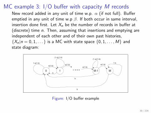
MC example 3: I/O buffer with capacity M recordsNew record added in any unit of time w.p. α (if not full). Bufferemptied in any unit of time w.p β. If both occur in same interval,insertion done first. Let Xn be the number of records in buffer at(discrete) time n. Then, assuming that insertions and emptying areindependent of each other and of their own past histories,Xn|n = 0, 1, . . . is a MC with state space 0, 1, . . . ,M andstate diagram:
0 1 M-1 M
a(1-b) a(1-b) a(1-b)
a(1-b)
(1-a)(1-b) (1-a)(1-b)
1-b 1-a(1-b)
b
b
b
Figure: I/O buffer example
30 / 226

MC example 3: I/O buffer with capacity M records
The transition matrix follows immediately, e.g.
q12 = α(1− β) = qn,n+1 (0 ≤ n ≤ M − 1)
qMM = 1− β
31 / 226

Markov chain two-step transition probabilities
Let
q(2)ij = P(Xn+2 = j |Xn = i)
=∑k∈Ω
P(Xn+1 = k,Xn+2 = j |Xn = i) from law of tot. prob.
=∑k∈Ω
P(Xn+2 = j |Xn = i ,Xn+1 = k)P(Xn+1 = k |Xn = i)
=∑k∈Ω
P(Xn+2 = j |Xn+1 = k)P(Xn+1 = k |Xn = i) by MP
=∑k∈Ω
qikqkj by TH
= (Q2)ij
32 / 226

Markov chain multi-step transition probabilities
Similarly, m-step transition probabilities :
q(m)ij = P(Xn+m = j |Xn = i) (m ≥ 1)
= (Qm)ij
by induction on m. Therefore we can compute probabilisticbehaviour of a MC over any finite period of time, in principle. E.g.average no. of records in buffer at time 50
E [X50|X0 = 0] =
min(M,50)∑j=1
jq(50)0j .
33 / 226

Long term behaviour
Markov chain multi-step transition probabilities can becomputationally intractable. We wish to determine long-termbehaviour: hope that asymptotically MC approaches a steady-state(probabilistically), i.e. that ∃pj |j = 0, 1, 2, . . . s.t.
pj = limn→∞
P(Xn = j |X0 = i) = limn→∞
q(n)ij
independent of i .
34 / 226

Definitions and properties of MCs
Let vij = prob. that state j will eventually be entered, given thatthe MC has been in state i , i.e.
vij = P(Xn = j for some n|X0 = i)
I If vij 6= 0, then j is reachable from i
I If vij = 0 ∀j 6= i , vii = 1, then i is an absorbing state
Example (1) & (3): all states reachable from each other (e.g. lookat transition diagrams)Example (2): all states in 1, 2, . . . , 99 reachable from each other,0 & 100 absorbing
35 / 226

Closed and irreducible MCsA subset of states, C is called closed if j /∈ C , implies j cannot bereached from any i ∈ C . E.g. set of all states, Ω, is closed. If 6 ∃proper subset C ⊂ Ω which is closed, the MC is called irreducible.A Markov Chain is irreducible if and only if every state is reachablefrom every other state. E.g. examples (1) & (3) and 0, 100are closed in example (2).
S1
S3
S4
S2
S5
S6
Reducible
S1
S3
S4
S2
S5
S6
Irreducible
36 / 226

Recurrent states
If vii = 1, state i is recurrent (once entered, guaranteed eventuallyto return). Thus we have:i recurrent implies i is either not visited by the MC or is visited aninfinite number of times – no visit can be the last (with non-zeroprobability).If i is not recurrent it is called transient. This implies the numberof visits to a transient state is finite w.p. 1 (has geometricdistribution). E.g. if C is a closed set of states, i /∈ C , j ∈ C andvij 6= 0, then i is transient since MC will eventually enter C from i ,never to return. E.g. in example (2), states 1 to 99 are transient,states 0 and 100 are recurrent (as is any absorbing state)
37 / 226
Proposition
If i is recurrent and j is reachable from i, then j is also recurrent.
Proof.vjj 6= 1 implies vij 6= 1 since if the MC visits i after j it will visit irepeatedly and with probability 1 will eventually visit j sincevij 6= 0. This implies vii 6= 0 since with non-zero probability theMC can visit j after i but not return to i (w.p. 1− vji > 0).
Thus, in an irreducible MC, either all states are transient (atransient MC) or recurrent (a recurrent MC).
38 / 226

Further properties of MCs
Let X be an irreducible, recurrent MC and let nj1, n
j2, . . . be the
times of successive visits to state j , mj = E [njk+1 − nj
k ](k = 1, 2, . . . ), the mean interval between visits (independent of kby the MP).Intuition:
pj =1
mj
Because the proportion of time spent, on average, in state j is1/mj .This is not necessarily true, because the chain may exhibit someperiodic behaviour:
The state j is periodic with period m > 1 if q(k)ii = 0 for k 6= rm
for any r ≥ 1 and P(Xn+rm = j for some r ≥ 1|Xn = j) = 1.Otherwise it is aperiodic, or has period 1. (Note that a periodicstate is recurrent)
39 / 226

Periodicity in an irreducible MC
Proposition
In an irreducible MC, either all states are aperiodic or periodic withthe same period. The MC is then called aperiodic or periodicrespectively.
Proposition
If Xn|n = 0, 1, . . . is an irreducible, aperiodic MC, then thelimiting probabilities pj |j = 0, 1, . . . exist and pj = 1/mj .
40 / 226

Null and positive recurrence
If mj =∞ for state j then pj = 0 and state j is recurrent null.Conversely, if mj <∞, then pj > 0 and state j is recurrentnon-null or positive recurrent.
Proposition
In an irreducible MC, either all states are positive recurrent or noneare. In the former case, the MC is called positive recurrent (orrecurrent non-null).
41 / 226

A state which is aperiodic and positive recurrent is often calledergodic and an irreducible MC whose states are all ergodic is alsocalled ergodic. When the limiting probabilities pj |j = 0, 1, . . . doexist they form the
steady state
equilibrium
long term
probability distribution (SSPD)
of the MC. They are determined by the following theorem.
42 / 226
Steady state theorem for Markov chains
TheoremAn irreducible, aperiodic Markov Chain, X , with state space S andone-step transition probability matrix Q = (qij |i , j ∈ S), is positiverecurrent if and only if the system of equations
pj =∑i∈S
piqij
with∑
i∈S pi = 1 (normalisation) has a solution. If it exists, thesolution is unique and is the SSPD of X .
43 / 226
NoteIf S is finite, X is always positive recurrent, which implies theequations have a unique solution. The solution is then found bydiscarding a balance equation and replacing it with the normalisingequation (the balance equations are dependent since the rows ofhomogeneous equations p− pQ = 0 all sum to zero).
44 / 226

MC example 3: Discrete time buffer
1 ≤ i ≤ M − 1From the steady state theorem:
pi = α(1− β)pi−1 + pi (1− α)(1− β)
i.e.(α(1− β) + β)pi = α(1− β)pi−1
which is equivalent to the heuristic “flow balance“ view (cf.CTMCs later):
Probability of leaving state i = Probability of entering state i
Thereforepi = kpi−1 = k ip0
where k = α(1−β)α+β−αβ (1 ≤ i ≤ M − 1).
45 / 226

Discrete time buffer state transition diagram
0 1 M-1 M
a(1-b) a(1-b) a(1-b)
a(1-b)
(1-a)(1-b) (1-a)(1-b)
1-b 1-a(1-b)
b
b
b
Figure: I/O buffer.
46 / 226

i = MβpM = α(1− β)pM−1
therefore
pM =α(1− β)
βkM−1p0
i = 0Redundant equation (why?) – use as check
α(1− β)p0 =M∑i=1
βpi = β
M−1∑i=1
k ip0 + kM−1α(1− β)p0
= p0
(βk
1− kM−1
1− k+ α(1− β)kM−1
)rest is exercise
47 / 226
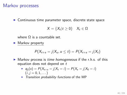
Markov processes
I Continuous time parameter space, discrete state space
X = Xt |t ≥ 0 Xt ∈ Ω
where Ω is a countable set.
I Markov property
P(Xt+s = j |Xu, u ≤ t) = P(Xt+s = j |Xt)
I Markov process is time homogeneous if the r.h.s. of thisequation does not depend on t
I qij(s) = P(Xt+s = j |Xt = i) = P(Xs = j |X0 = i)(i , j = 0, 1, . . . )
I Transition probability functions of the MP
48 / 226

Memoryless property
Markov Property and time homogeneity imply:If at time t the process is in state j , the time remaining in state jis independent of the time already spent in state j : memorylessproperty
49 / 226

Proof.
P(S > t + s|S > t) = P(Xt+u = j , 0 ≤ u ≤ s|Xu = j , 0 ≤ u ≤ t)
where S = time spent in state j ,
state j entered at time 0
= P(Xt+u = j , 0 ≤ u ≤ s|Xt = j) by MP
= P(Xu = j , 0 ≤ u ≤ s|X0 = j) by T.H.
= P(S > s)
=⇒ P(S ≤ t + s|S > t) = P(S ≤ s)
Time spent in state i is exponentially distributed, parameter µi .
50 / 226

Time homogeneous Markov Processes
The MP implies next state, j , after current state i depends only oni , j – state transition probability qij . This implies the MarkovProcess is uniquely determined by the products:
aij = µiqij
where µi is the rate out of state i and qij is the probability ofselecting state j next. The aij are the generators of the MarkovProcess.
I intuitively reasonable
51 / 226

Instantaneous transition rates
Consider now the (small) interval (t, t + h)
P(Xt+h = j |Xt = i) = µihqij + o(h)
= aijh + o(h)
I aij is the instantaneous transition rate i → j i.e. the averagenumber of transitions i → j per unit time spent in state i
52 / 226

MP example: a Poisson process
aij =
λ if j = i + 1
0 if j 6= i , i + 1
not defined if j = i
becauseP(arrival in (t, t + h))︸ ︷︷ ︸
i→i+1
= λh︸︷︷︸ai,i+1h
+o(h)
53 / 226

MP example: The buffer problem
I Records arrive as a P.P. rate λ
I Buffer capacity is M
I Buffer cleared at times spaced by intervals which areexponentially distributed, parameter µ. Clearance times i.i.d.and independent of arrivals (i.e. clearances are anindependent PP, rate µ)
aij =
λ if j = i + 1 (0 ≤ i ≤ M − 1)
µ if j = 0 (i 6= 0)
0 otherwise (j 6= i)
[Probability of > 1 arrivals or clearances, or ≥ 1 arrivals andclearances in (t, t + h) is o(h)]
54 / 226
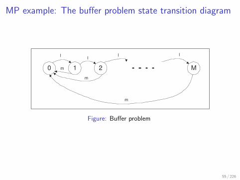
MP example: The buffer problem state transition diagram
0 1 2 M
l
m
m
m
l l l
Figure: Buffer problem
55 / 226

MP example: Telephone exchangeSuppose there 4 subscribers and any two calls between differentcallers can be supported simultaneously. Calls are made bynon-connected subscribers according to independent PPs, rate λ(callee chosen at random). Length of a call is (independent)exponentially distributed, parameter µ. Calls are lost if calledsubscriber is engaged. State is the number of calls in progress (0,1or 2).
a01 = 4λ (all free)
a12 =2
3λ (caller has
1
3probability of successful connection)
a10 = µ
a21 = 2µ (either call may end)
0 1 2
m 2m
4l 2/3 l
56 / 226

Exercise
The last equation follows because the distribution of the randomvariable Z = min(X ,Y ) where X ,Y are independent exponentialrandom variables with parameters λ, µ respectively is exponentialwith parameter λ+ µ. Prove this.
57 / 226

The generator matrix
∑j∈Ω,j 6=i
qij = 1 =⇒ µi =∑
j∈Ω,j 6=i
aij
(hence instantaneous transition rate out of i). Let aii = −µi
(undefined so far)
(aij) = A =
a00 a01 . . .a10 a11 . . .. . .ai0 ai1 . . . aii . . .. . .
A is the generator matrix of the Markov Process. Rows of A sumto zero (
∑j∈S aij = 0)
58 / 226

Transition probabilities and rates
I determined by A
qij =aij
µi= −
aij
aii
µi = −aii
I hence A is all we need to determine the Markov processI Markov processes are instances of state transition systems
with the following propertiesI The state holding time are exponentially distributedI The probability of transiting from state i to state j depends
only on i and j
I In order for the analysis to work we require that the process inirreducible – every state must be reachable from every other,e.g.
59 / 226

Steady state results
Theorem
(a) if a Markov process is transient or recurrent null,pj = 0 ∀j ∈ S and we say a SSPD does not exist
(b) If a Markov Process is positive recurrent, the limits pj exist,pj > 0,
∑j∈S pj = 1 and we say pj |j ∈ S constitute the
SSPD of the Markov Process.
60 / 226

Steady state theorem for Markov processes
TheoremAn irreducible Markov Process X with state space S and generatormatrix A = (aij) (i , j ∈ S) is positive recurrent if and only if∑
i∈S
piaij = 0 for j ∈ S [Balance equations]∑i∈S
pi = 1 [Normalising equation]
have a solution. This solution is unique and is the SSPD.
NoteAt equilibrium the fluxes also balance into and out of every closedcontour drawn around any collection of states.
61 / 226

Justification of the balance equation
The rate going from state i to j(6= i) is aij , the fraction of timespent in i is pi∑
i 6=j
aijpi︸ ︷︷ ︸Avg. no. of transitions i→j in unit time
=∑i 6=j
ajipj︸ ︷︷ ︸Avg. no. of transitions j→i in unit time∑
i 6=j
flux(i → j) =∑i 6=j
flux(j → i) ∀j
62 / 226

MP example: I/O bufferBy considering the flux into and out of each state 0, 1, . . . ,M weobtain the balance equations:
λp0 = µ(p1 + · · ·+ pM) (State 0)
(λ+ µ)pi = λpi−1 (State i , for 1 ≤ i ≤ M − 1)
µpM = λpM−1 (State M)
Normalising equation:
p0 + p1 + · · ·+ pM = 1
=⇒ pj =( λ
λ+ µ
)j µ
λ+ µ(for 0 ≤ j ≤ M − 1)
pM =( λ
λ+ µ
)M
Thus (for example) mean number of records in the buffer in thesteady state = MαM +
∑M−1j=0 jαj µ
λ+µ where α = µλ+µ
63 / 226

MP example: Telephone network
4λp0 = µp1 (State 0)(µ+
2
3λ)
p1 = 4λp0 + 2µp2 (State 1)
2µp2 = λ2
3p1 (State 2)
Thus p1 = 4λµ p0, p2 = λ
3µp1 = 4λ2
3µ2 p0 with
p0 + p1 + p2 = 1 =⇒ p0 =(
1 +4λ
µ+
4λ2
3µ2
)−1.
Average number of calls in progress in the steady state
= 1.p1 + 2.p2 =4λµ
(1+ 2λ
3µ
)1+ 4λ
µ+ 4λ2
3µ2
64 / 226

Birth-death processes and the single server queue (SSQ)
A Markov process with state space S = 0, 1, . . . is called abirth-death process if the only non-zero transition probabilities areai ,i+1 and ai+1,i (i ≥ 0), representing births and deathsrespectively. (In a population model, a00 would be 1 since 0 wouldbe an absorbing state.) The SSQ model consists of
I a Poisson arrival process, rate λ
I a queue which arriving tasks join
I a server which processes tasks in the queue in FIFO (or other)order and has exponentially distributed service times,parameter µ (i.e. given a queue length > 0, servicecompletions form a Poisson process, rate µ)
65 / 226
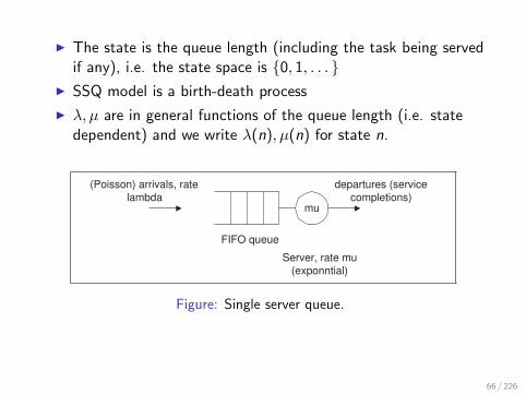
I The state is the queue length (including the task being servedif any), i.e. the state space is 0, 1, . . .
I SSQ model is a birth-death process
I λ, µ are in general functions of the queue length (i.e. statedependent) and we write λ(n), µ(n) for state n.
mu
(Poisson) arrivals, rate
lambda
FIFO queue
Server, rate mu
(exponntial)
departures (service
completions)
Figure: Single server queue.
66 / 226

Kendall’s notation
NotationThe SSQ with Poisson arrivals and exponential service times iscalled an M/M/1 queue
I the first M describes the arrival process as a Markov process(Poisson)
I the second M describes the service time distribution as aMarkov process (exponential)
I the 1 refers to a single server (m parallel server would bedenoted as M/M/m)
I Later we will consider M/G/1 queues, where the service timedistribution is non-Markovian (“general”)
67 / 226

The memoryless property in the M/M/1 queue
SSQ therefore follows a Markov process and has the memorylessproperty that:
1. Probability of an arrival in (t, t + h) = λ(i)h + o(h) in state i
2. Probability of a service completion in(t, t + h) = µ(i)h + o(h) in state i > 0 (0 if i = 0)
3. Probability of more than 1 arrival, more than one servicecompletion or 1 arrival and 1 service completion in(t, t + h) = o(h).
4. Form these properties we could derive a differential equationfor the transient queue length probabilities – compare Poissonprocess.
68 / 226

State transition diagram for the SSQ
0 1 i i+1
l(0) l(1) l(i-1) l(i) l(i+1)
m(i+2) m(i+1) m(i) m(2) m(1)
Figure: Single server queue state diagram.
69 / 226

I Consider the balance equation for states inside the red (thick)contour.
I Outward flux (all from state i): piλ(i) (i ≥ 0);I Inward flux (all from state i + 1): pi+1µ(i + 1) (i ≥ 0).
Thus,piλ(i) = pi+1µ(i + 1)
so
pi+1 =λ(i)
µ(i + 1)pi =
[ i∏j=0
ρ(j)]p0
where ρ(j) = λ(j)µ(j+1) .
70 / 226

I Normalising equation implies
p0
(1 +
∞∑i=0
i∏j=0
ρ(j))
= 1
so
p0 =[ ∞∑
i=0
i−1∏j=0
ρ(j)]−1
where∏−1
j=0 = 1 (the empty product). Therefore
pi =
∏i−1j=0 ρ(j)∑∞
k=0
∏k−1n=0 ρ(n)
(i ≥ 0).
I So, is there always a steady state?
71 / 226

I SSQ with constant arrival and service rates
λ(n) = λ, µ(n) = µ, ρ(n) = ρ = λ/µ ∀n ∈ S
implies
p0 =[ ∞∑
i=0
ρi]−1
= 1− ρ
pi = (1− ρ)ρi (i ≥ 0)
I Mean queue length, L (including any task in service)
L =∞∑i=0
ipi =∞∑i=0
(1− ρ)iρi
= ρ(1− ρ)d
dρ
∞∑i=0
ρi
= ρ(1− ρ)d
dρ
(1− ρ)−1
=
ρ
1− ρ
72 / 226

I Utilisation of server
U = 1− P(server idle) = 1− p0 = 1− (1− ρ) = ρ
= λ/µ.
However, we could have deduced this without solving for p0:In the steady state (assuming it exists),
λ = arrival rate
= throughput
= P(server busy).service rate
= Uµ
This argument applies for any system in equilibrium – wedidn’t use the Markov property – see M/G/1 queue later.
73 / 226
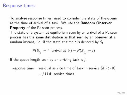
Response times
To analyse response times, need to consider the state of the queueat the time of arrival of a task. We use the Random ObserverProperty of the Poisson process.The state of a system at equilibrium seen by an arrival of a Poissonprocess has the same distribution as that seen by an observer at arandom instant, i.e. if the state at time t is denoted by St ,
P(St−0= i | arrival at t0) = P(St−0
= i)
If the queue length seen by an arriving task is j ,
response time = residual service time of task in service (if j > 0)
+ j i.i.d. service times
74 / 226

For exponential service times, residual service time has the samedistribution as full service time, so in this case
Response time = sum of (j + 1) i.i.d. service times.
Therefore, the mean response time, W is
W =∑
pj(j + 1)µ−1 =(
1 +ρ
1− ρ
)µ−1 =
1
µ− λ
and mean queueing time WQ (response time, excluding servicetime)
WQ = W − µ−1 = Lµ−1 =ρ
µ− λ.
75 / 226

Distribution of the waiting time, FW (x)
By the random observer property (and memoryless property)
FW (x) =∞∑j=0
pjEj+1(x)
where Ej+1(x) is the convolution of (j + 1) exponentialdistributions, each with parameter µ — called the Erlang–(j + 1)distribution with parameter µ. Similarly, for density functions:
fW (x) =∞∑j=0
pjej+1(x)
where ej+1(x) is the pdf corresponding to Ej+1(x), i.e.ddx Ej+1(x) = ej+1(x), defined by
76 / 226

e1(x) = µe−µx
ej+1(x) = µ
∫ x
0e−µ(x−u)ej(u)du︸ ︷︷ ︸
convolution of Erlang–j and exponential distributions
=⇒ ej(x) = µ(µx)j−1
(j − 1)!e−µx (Exercise)
=⇒ fW (x) = (µ− λ)e−(µ−λ)x (Exercise)
These results can be obtained much more easily using Laplacetransforms (which we will not detail here).
77 / 226

ExampleGiven m Poisson streams, each with rate λ and independent of theothers, into a SSQ, service rate µ, what is the maximum value ofm for which, in steady state, at least 95% of waiting times,W ≤ w? (Relevant in “end-to-end” message delays incommunication networks, for example.)That is, we seek m such that P(W ≤ w) ≥ 0.95
=⇒ 1− e−(µ−mλ)w ≥ 0.95
=⇒ e−(µ−mλ)w ≤ 0.05
=⇒ e(µ−mλ)w ≥ 20
=⇒ µ−mλ ≥ ln 20
w
=⇒ m ≤ µ
λ− ln 20
wλ
Notem < µ/λ is equivalent to the existence of a steady state.
78 / 226

Reversed processes
I The reversed process of a stochastic process is a dual processI with the same state spaceI in which the direction of time is reversedI cf. viewing a video film backwards.
I If the reversed process is stochastically identical to the originalprocess, that process is called reversible
79 / 226
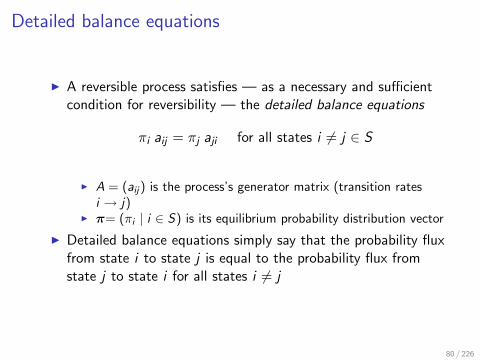
Detailed balance equations
I A reversible process satisfies — as a necessary and sufficientcondition for reversibility — the detailed balance equations
πi aij = πj aji for all states i 6= j ∈ S
I A = (aij) is the process’s generator matrix (transition ratesi → j)
I π= (πi | i ∈ S) is its equilibrium probability distribution vector
I Detailed balance equations simply say that the probability fluxfrom state i to state j is equal to the probability flux fromstate j to state i for all states i 6= j
80 / 226

Example — the M/M/1 queue
Recall our derivation of steady state probabilities for the M/M/1queue with state-dependent rates:
I Balancing probability flux into and out of the subset of states0, 1, . . . , i we found
πi ai ,i+1 = πi+1 ai+1,i
I There are no other classes of directly connected states
I Therefore the M/M/1 queue is reversible – including M/M/m,a special case of state-dependent M/M/1
81 / 226

Burke’s Theorem
Now consider the departure process of an M/M/1 queueI It is precisely the arrival process in the reversed queue
I remember, time is going backwardsI so, state decrements (departures) become increments (arrivals)
in the reversed process
I Since the reversed process is also an M/M/1 queue, itsarrivals are Poisson and independent of the past behaviour ofthe queue
I Therefore the departure process of the (forward or reversed)M/M/1 queue is Poisson and independent of the future stateof the queue
I Equivalently, the state of the queue at any time isindependent of the departure process before that time
82 / 226

Reversed Processes
I Most Markov processes are not reversible but we can stilldefine the reversed process X−t of any Markov process Xt atequilibrium
I It is straightforward to find the reversed process of a Markovprocess if its steady state probabilities are known:
I The reversed process of a Markov process Xt at equilibrium,with state space S , generator matrix A and steady stateprobabilities π, is a Markov process with generator matrix A′
defined bya′ij = πjaji/πi (i , j ∈ S)
and with the same stationary probabilities π
I So the flux from i to j in the reversed process is equal to theflux from j to i in the forward process, for all states i 6= j
83 / 226

Proof.For i 6= j and h > 0,
P(Xt+h = i)P(Xt = j |Xt+h = i) = P(Xt = j)P(Xt+h = i |Xt = j).
Thus,
P(Xt = j |Xt+h = i) =πj
πiP(Xt+h = i |Xt = j)
at equilibrium. Dividing by h and taking the limit h→ 0 yields therequired equation for a′ij when i 6= j . But, when i = j ,
−a′ii =∑k 6=i
a′ik =∑k 6=i
πkaki
πi=∑k 6=i
aik = −aii .
That π is also the stationary distribution of the reversed processnow follows since
−πia′ii = πi
∑k 6=i
aik =∑k 6=i
πka′ki .
84 / 226

Why is this useful?
In an irreducible Markov process, we may:
I Choose a reference state 0 arbitrarily
I Find a sequence of directly connected states 0, . . . , j
I calculate
πj = π0
j−1∏i=0
ai ,i+1
a′i+1,i
= π0
j−1∏i=0
a′i ,i+1
ai+1,i
I So if we can determine the matrix Q ′ independently of thesteady state probabilities π , there is no need to solve balanceequations.
85 / 226

RCAT, SPA and Networks
I A compositional result in Stochastic Process Algebra calledRCAT (Reversed Compound Agent Theorem) finds manyreversed processes and hence simple solutions for steady stateprobabilities
I open and closed queueing networksI multiple classes of customersI ‘negative customers’ that ‘kill’ customers rather than add to
them in a queueI batches and other synchronized processes
I Automatic or mechanised, unified implementation
I Hot research topic – see later in the course!
86 / 226
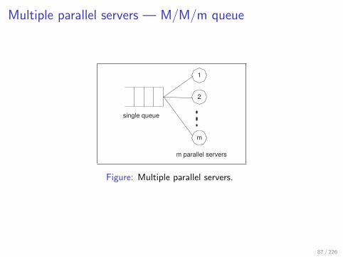
Multiple parallel servers — M/M/m queue
1
2
m
single queue
m parallel servers
Figure: Multiple parallel servers.
87 / 226

M/M/m SSQSSQ representation:
λ(n) = λ (n ≥ 0)
µ(n) =
nµ 1 ≤ n ≤ m
mµ n ≥ m
The front of the queue is served by any available server.
By a general result for the M/M/1 queue:
pj = p0
j−1∏i=0
λ(i)
µ(i + 1)=
p0
ρj
j! 0 ≤ j ≤ m
p0ρj
m!mj−m j ≥ m
so
p0 =1∑m−1
i=0ρi
i! + ρm
m!
∑∞i=m( ρm )i−m
=1∑m−1
i=0ρi
i! + ρm
(m−1)!(m−ρ)
.
88 / 226

Average number of busy servers, S
S =m−1∑k=1
kpk + m∞∑
k=m
pk = · · · = ρ
Steady state argument
arrival rate = λ
average throughput = Sµ (µ per active server)
=⇒ Sµ = λ (in equilibrium).
Utilisation U = S/m = ρ/m, the average fraction of busy servers.
89 / 226

Waiting times
Waiting time is the same as service time if an arrival does not haveto queue. Otherwise, the departure process is Poisson, rate mµ,whilst the arrived task is queueing (all servers busy). This impliesthat the queueing time is the same as the queueing time in theM/M/1 queue with service rate mµ.
I Let
q = P(arrival has to queue)
= P(find ≥ m jobs on arrival)
I by R.O.P.
q =∞∑
j=m
pj = p0ρm
(m − 1)!(m − ρ)Erlang delay formula
90 / 226

I Let Q be the queueing time random variable (excludingservice)
FQ(x) = P(Q ≤ x) = P(Q = 0) + P(Q ≤ x |Q > 0)P(Q > 0)
= (1− q) + q(1− e−(mµ−λ)x)
= 1− qe−(mµ−λ)x
P(Q ≤ x |Q > 0) is given by the SSQ, rate mµ, result forwaiting time. (Why is this?)Note that FQ(x) has a jump at the origin, FQ(0) 6= 0.
I Mean queueing time
WQ =q
mµ− λI Mean waiting time
W = WQ + 1/µ =(q + m)µ− λµ(mµ− λ)
I Exercise: What is the waiting time density function?
91 / 226

The infinite server
I In the M/M/m queue, let m→∞I “unlimited service capacity”I always sufficient free servers to process an arriving task - e.g.
when the number tasks in the system is finiteI no queueing =⇒ infinite servers model delays in a task’s
processing
pj =ρj
j!p0 =⇒ p0 = e−ρ
I balance equations have a solution for all λ, µI this is not surprising since the server can never be overloaded
I This result is independent of the exponential assumption – aproperty of the queueing discipline (here there is no queueing– a pathological case)
92 / 226

M/M/m queues with finite state space
M/M/1/k (k is the max. queue length) queue
µ(n) = nµ for all queue lengths n
λ(n) =
λ 0 ≤ n < k
0 n ≥ k
Hence, if ρ = λ/µ.
pj =
p0ρj j = 0, 1, . . . , kQj−1i=0 λ(i)Qj−1
i=0 µ(i+1)= 0 j > k (as λ(k) = 0)
93 / 226
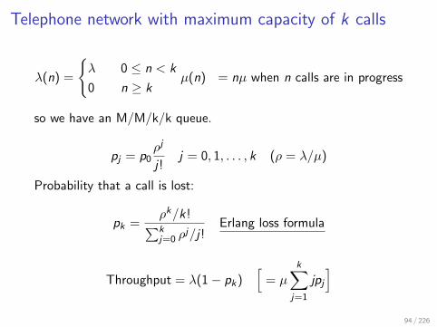
Telephone network with maximum capacity of k calls
λ(n) =
λ 0 ≤ n < k
0 n ≥ kµ(n) = nµ when n calls are in progress
so we have an M/M/k/k queue.
pj = p0ρj
j!j = 0, 1, . . . , k (ρ = λ/µ)
Probability that a call is lost:
pk =ρk/k!∑kj=0 ρ
j/j!Erlang loss formula
Throughput = λ(1− pk)[
= µ
k∑j=1
jpj
]94 / 226

Terminal system with parallel processing
N users logged on to a computer system with m parallel processors
I exponentially distributed think times, mean 1/λ, beforesubmitting next task
I each processor has exponential service times, mean 1/µ
Single Queue
.
.
.
P1
P2
Pm
(0≤n≤N tasks)
.
.
.
T1
T2
TN
Figure: Terminals with parallel processors.
95 / 226

I tasks may use any free processor, or queue (FIFO) if there arenone.
I state space S = n|0 ≤ n ≤ N where n is the queue length(for all processors)
I Poisson arrivals, rate λ(n) = (N − n)λ
I Service rate µ(n) =
nµ 1 ≤ n ≤ m
mµ m ≤ n ≤ N
96 / 226
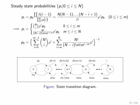
Steady state probabilities pi |0 ≤ i ≤ N
pi = p0
∏λ(i − 1)∏µ(i)
=N(N − 1) . . . (N − i + 1)
i !ρip0 (0 ≤ i ≤ m)
=⇒ pi =
(Ni
)ρip0 0 ≤ i ≤ m
N!(N−i)!m!mi−m ρ
ip0 m ≤ i ≤ N
p0 =m−1∑
i=0
(N
i
)ρi +
N∑i=m
N!
(N − i)!m!mi−mρi−1
0 1 m-1 m N
Nl (N-1)l (N-m+2)l (N-m+1)l l (N-m)l
mmu mmu mmu (m-1)mu 2mu
mu
Figure: State transition diagram.
97 / 226

The throughput is either given by
µm−1∑
j=1
jpj + mN∑
j=m
pj
(mean departure rate from processors)
or
λ
N −N∑
j=1
jpj
(mean arrival rate)
Other performance measures as previously
98 / 226

The case of “always sufficient processors” - m ≥ N
I Here there is no case m < i ≤ N
=⇒ pi =
(N
i
)ρip0 (0 ≤ i ≤ N)
=⇒ p0 = N∑
i=0
(N
i
)ρi−1
= (1 + ρ)−N
Thus pi =
(N
i
)( ρ
1 + ρ
)i( 1
1 + ρ
)N−i
(Binomial distribution)
99 / 226

I Probabilistic explanationI pi is the probability of i “successes” in N Bernoulli (i.i.d.) trialsI probability of success = ρ
1+ρ = 1/µ1/λ+1/µ = fraction of time
user is waiting for a task to complete in the steady state =probability (randomly) observe a user in wait-mode.
I probability of failure = fraction of time user is in think mode inthe steady state = probability (randomly) observe a user inthink-mode
I random observations are i.i.d. in steady state =⇒ trials areBernoulli
I hence Binomial distribution
I result is independent of distribution of think times.
100 / 226

Analogy with a queueing network
Regard the model as a 2-server, cyclic queueing network
T1 P1
TN PM
tasks N n 0 no queueing
=⇒
P T
infinite server Multi-server
Figure: Original and equivalent network.
I As already observed, IS server is insensitive to its service timedistribution as far as queue length distribution is concerned.
I Multi-server becomes IS if M ≥ N =⇒ 2 IS servers.
101 / 226

Little’s result/formula/law (J.D.C. Little, 1961)
Suppose that a queueing system Q is in steady state (i.e. there arefixed, time independent probabilities of observing Q in each of itspossible states at random times.) Let:
L = average number of tasks in Q in steady state
W = average time a task spends in Q in steady state
λ = arrival rate (i.e. average number of tasks entering
or leaving Q in unit time)
ThenL = λW .
102 / 226

Intuitive Justification
Suppose a charge is made on a task of £1 per unit time it spendsin Q
I Total collected on average in unit time = L
I Average paid by one task = W
I If charges collected on arrival (or departure), average collectedin unit time = λ.W
=⇒ L = λW
I Example: M/M/1 queue
W = (L + 1)/µ by R.O.P.
L = λW =⇒ W =1
µ− λ
103 / 226

Application of Little’s law
Server utilisation U.
Figure: Little’s law.
104 / 226

I Consider server, rate µ (constant), inside some queueingsystem: i.e. average time for one service = 1/µ
I Let total throughput of server = λ = total average arrival rate(since in steady state)
I Apply Little’s result to the server only (without the queue)
mean queue length = 0.P(idle) + 1.P(busy)
= U
mean service time = µ−1
=⇒ U =λ
µ
I Not the easiest derivation! This is a simple work conservationlaw.
105 / 226

Single server queue with general service times: the M/G/1queue
Assuming that arrivals are Poisson with constant rate λ, servicetime distribution has constant mean µ−1 (service rate µ) and thata steady state exists
Utilisation, U = P(queue length > 0)
=µ−1
λ−1= λ/µ = “load.”
(For an alternate viewpoint, utilisation may be seen as the averageamount of work arriving in unit time; we already know this, ofcourse.)
106 / 226
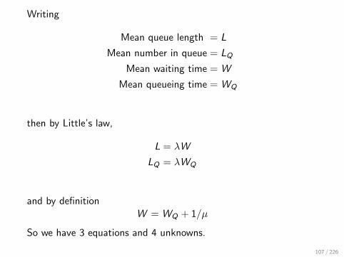
Writing
Mean queue length = L
Mean number in queue = LQ
Mean waiting time = W
Mean queueing time = WQ
then by Little’s law,
L = λW
LQ = λWQ
and by definitionW = WQ + 1/µ
So we have 3 equations and 4 unknowns.
107 / 226
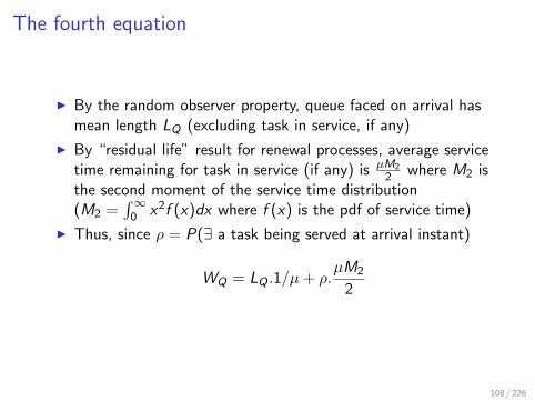
The fourth equation
I By the random observer property, queue faced on arrival hasmean length LQ (excluding task in service, if any)
I By “residual life” result for renewal processes, average servicetime remaining for task in service (if any) is µM2
2 where M2 isthe second moment of the service time distribution(M2 =
∫∞0 x2f (x)dx where f (x) is the pdf of service time)
I Thus, since ρ = P(∃ a task being served at arrival instant)
WQ = LQ .1/µ+ ρ.µM2
2
108 / 226

I Now
LQ = λWQ =⇒ LQ ,WQ , L,W
L = ρ+λ2M2
2(1− ρ)
I Observe that if standard deviationmean (and hence the second
moment) of service time distribution is large, L is also (nottrivial as M2 increases with µ−1 - but not difficult either!)
109 / 226

Embedded Markov chain
I State of the M/G/1 queue at time t is X (t) ∈ S where thestate space S = n|n ≥ 0 as in M/M/1 queue.
I M/G/1 queue is not a Markov processI P(X (t + s)|X (u), u ≤ t) 6= P(X (t + s)|X (t)) ∀t, sI e.g. if a service period does not begin at time tI no memoryless property
I Consider times t1, t2, . . . of successive departures and letXn = X (t+
n )
110 / 226

I Given Xi , X (t) for t > ti is independent of X (t ′) for t ′ < tisince at time t+
iI time to next arrival is exponential with parameter λ because
arrival process is PoissonI instantaneously, no task is in service, so time to next departure
is a complete service time or that plus the time to next arrival(if queue empty)
=⇒ Xi |i ≥ 1 is a Markov Chain with state space S(ti |i ≥ 1 are called “Markov times”)
I It can be shown that, in steady state of E.M.C., distributionof no. of jobs, j , “left behind” by a departure = distributionof no. of jobs, j , seen by an arrival = limn→∞ P(Xn = j) byR.O.P.
I Here we solve pj =∑∞
n=0 pnqnj (j ≥ 0) for appropriateone-step transition probabilities qij .
111 / 226

Balance equations for the M/G/1 queue
I Solution for pj exists iff ρ = λµ < 1, equivalent to p0 > 0
since p0 = 1− U = 1− ρ in the steady state.
I Valid one-step transitions are i → j forj = i − 1, i , i + 1, i + 2, . . . since we may have an arbitrarynumber of arrivals between successive departures.
I Letrk = P(k arrivals in a service period)
then
qij = P(Xn+1 = j |Xn = i) n ≥ 0
= rj−i+1︸ ︷︷ ︸because i→i−1+(j−i+1)
i ≥ 1, j ≥ i − 1
q0j = rj j ≥ 0
112 / 226

[Eventually a job arrives, so 0→ 1, and then 1→ j if there are jarrivals in its service time since then 1→ 1− 1 + j = j ]
=⇒ p0 = 1− ρ
pj = p0rj +
j+1∑i=1
pi rj−i+1 (j ≥ 0)
where rk =∫∞
0λx)k
k! e−λx f (x)dx if service time density function isf (x) (known). This is because
P(k arrivals in service time|service time = x) = λx)k
k! e−λx andP(service time ∈ (x , x + dx)) = f (x)dx
113 / 226

Solutions to the balance equations
I In principle we could solve the balance equations by “forwardsubstitution”
I p0 is knownI j = 0: p0 allows us to find p1
I j = 1: p0, p1 allow us to find p2
...
I j = i : p0, p1, . . . , pi allow us to find pi+1
but computationally this is impractical in general
114 / 226

I Define generating functions
p(z) =∞∑i=0
pizi
r(z) =∞∑i=0
rizi
Recap:
p′(z) =∞∑i=1
ipizi−1
=⇒ p′(1) = mean value of distribution pj |j ≥ 0
p′′(z) =∞∑i=2
(i2 − i)pizi−2
=⇒ p′′(1) = M2 −M1
115 / 226

I Multiply balance equations by z j and sum:
p(z) = p0r(z) +∞∑j=0
j+1∑i=1
pi rj−i+1z j
= p0r(z) + z−1∞∑i=0
∞∑j=0
pi+1z i+1rj−izj−i
where rk = 0 for k < 0
= p0r(z) + z−1∞∑i=0
pi+1z i+1∞∑j=0
rj−izj−i
= p0r(z) + z−1(p(z)− p0)r(z)
116 / 226

Solution for p(z) and the Pollaczek-Khinchine result
p(z) =p0(1− z)r(z)
r(z)− z
where r(z) =
∫ ∞0
∞∑k=0
(λxz)k
k!e−λx f (x)dx
=
∫ ∞0
e−λx(1−z)f (x)dx
= f ∗(λ− λz)
which is the Laplace transform of f at the point λ− λz
117 / 226

Recap: Laplace transform f ∗ of f defined by
f ∗(s) =
∫ ∞0
e−sx f (x)dx
so thatdn
dsnf ∗(s) =
∫ ∞0
(−x)ne−sx f (x)dx
=⇒ dnf ∗(s)
dsn
∣∣∣s=0
= (−1)nMn nth moment of f (x)
E.g. f ∗(0) = 1, −f ∗′(0) = mean service time = 1/µ. Thus,
p(z) =(1− ρ)(1− z)f ∗(λ− λz)
f ∗(λ− λz)− z
p′(1) =⇒ P-K formula . . .
118 / 226
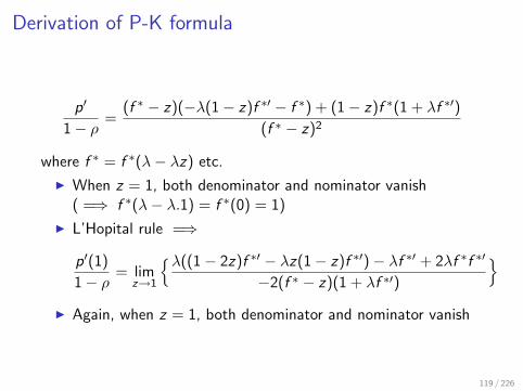
Derivation of P-K formula
p′
1− ρ=
(f ∗ − z)(−λ(1− z)f ∗′ − f ∗) + (1− z)f ∗(1 + λf ∗′)
(f ∗ − z)2
where f ∗ = f ∗(λ− λz) etc.
I When z = 1, both denominator and nominator vanish( =⇒ f ∗(λ− λ.1) = f ∗(0) = 1)
I L’Hopital rule =⇒
p′(1)
1− ρ= lim
z→1
λ((1− 2z)f ∗′ − λz(1− z)f ∗′)− λf ∗′ + 2λf ∗f ∗′
−2(f ∗ − z)(1 + λf ∗′)
I Again, when z = 1, both denominator and nominator vanish
119 / 226

I L’Hopital rule now gives
p′(1)
1− ρ=λ(−2f ∗′(0) + λf ∗′′(0)− 2λf ∗′(0)2)
2(1 + λf ∗′(0))2
(since f ∗(0) = 1)
=λ2M2 + 2(λ/µ)(1− (λ/µ))
2(1− (λ/µ))2P-K formula!
(since f ∗′(0) = 1/µ)
I Hard work compared to previous derivation! But in principlewe could obtain any moment (“well known” result for varianceof queue length)
120 / 226

Waiting time distribution
I The tasks left in an M/G/1 queue on departure of a giventask are precisely those which arrived during its waiting time
=⇒ pj =
∫ ∞0
(λx)j
j!e−λxh(x)dx
because P(j arrivals|waiting time = x) =(λx)j
j!e−λx
P(waiting time ∈ (x , x + dx)) = h(x)dx
=⇒ p(z) = h∗(λ− λz)
by the same reasoning as before.
121 / 226

I Laplace transform of waiting time distribution is therefore (letz = λ−s
λ )
h∗(s) = p(λ− s
λ
)=
(1− ρ)sf ∗(s)
λf ∗(s)− λ+ s
I Exercise: Verify Little’s Law for the M/G/1 queue:
p′(1) = −λh∗′(0).
122 / 226

Example: Disk access time model
track queue
head (one for each track)
n equal sized sectors
(records) per track
Figure: Fixed head disk.
123 / 226
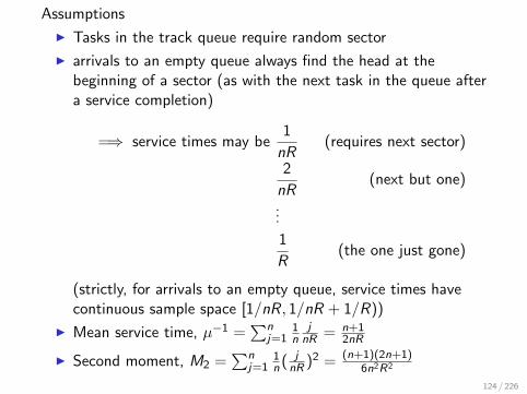
Assumptions
I Tasks in the track queue require random sector
I arrivals to an empty queue always find the head at thebeginning of a sector (as with the next task in the queue aftera service completion)
=⇒ service times may be1
nR(requires next sector)
2
nR(next but one)
...
1
R(the one just gone)
(strictly, for arrivals to an empty queue, service times havecontinuous sample space [1/nR, 1/nR + 1/R))
I Mean service time, µ−1 =∑n
j=11n
jnR = n+1
2nR
I Second moment, M2 =∑n
j=11n ( j
nR )2 = (n+1)(2n+1)6n2R2
124 / 226

Solution and asymptotic behaviour
I Load is ρ = λ/µ = λ(n+1)2nR =⇒ λ < 2nR
n+1 if drum track is notto be saturated
I Mean queue length, L = ρ+ λ2(n+1)(2n+1)12n2R2(1−ρ)
I As n→∞, i.e. many sectors on trackI assumption about arrivals to an empty queue becomes exact
(large n =⇒ good approximation)I ρ→ λ
2R
I L→ λ2R + λ2
3R(2R−λ)
125 / 226

Queueing Networks
I Collection of servers/queues interconnected according to sometopology
1
3 5
2 4 departures
departures
external arrivals
Figure: Network example
126 / 226

I Servers may beI processing elements in a computer, e.g. CPU I/O devicesI stations/nodes in a communication network (may be widely
separated geographically)
I Topology represents the possible routes taken by tasksthrough the system
I May be several different classes of tasks (multi-class network)I different service requirements at each nodeI different routing behavioursI more complex notation, but straightforward generalisation of
the single-class network in principleI we will consider only the single class case
127 / 226

Types of network
I Open: at least one arc coming from the outside and at leastone going out
I must be at least one of each type or else the network would besaturated or null (empty in the steady state)
I e.g. the example above
I Closed: no external (incoming or outgoing) arcI constant network population of tasks forever circulatingI e.g. the example above with the external arcs removed from
nodes 1 and 4
I Mixed: multi-class model which is open with respect to someclasses and closed with respect to others – e.g. in the exampleabove a class whose tasks only ever alternated between nodes2 and 4 would be closed, whereas a class using all nodeswould be open
128 / 226

Types of server
I Server defined by its service time distribution (we assumeexponential but can be general for non-FCFS disciplines) andits queueing discipline (for each class)
I FCFS (FIFO)I LCFS (LIFO)I IS (i.e. a delay node: no queueing)I PS (Processor sharing: service shared equally amongst all tasks
in the queue)
I Similar results for queue length probabilities (in S.S.) for all
129 / 226

Open networks (single class)
I Notation:M servers, 1, 2, . . . ,M with FCFS discipline and exponentialservice times, mean 1
µi (ni ), when queue length is ni
(1 ≤ i ≤ M)I state dependent service rates to a limited extentI µi (nj) for i 6= j =⇒ blocking: rate at one server depends on
the state of another, e.g. rate → 0 when finite queue at next isfull
I External Poisson arrivals into node i , rate γi , (1 ≤ i ≤ M)(= 0 if no arrivals)
130 / 226

I Routing probability matrix Q = (qij |1 ≤ i ≤ M)I qij = probability that on leaving node i a task goes to node j
independently of past historyI qi0 = 1−
∑Mj=1 qij = probability of external departure from
node iI at least one qi0 > 0, i.e. at least one row of Q sums to less
than 1
I State space of network S = (n1, . . . , nM)|ni ≥ 0I queue length vector random variable is (N1, . . . ,NM)I p(n) = p(n1, . . . , nM) = P(N1 = n1, . . . ,NM = nM)
131 / 226
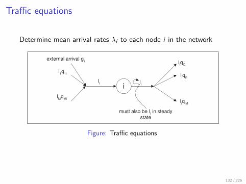
Traffic equations
Determine mean arrival rates λi to each node i in the network
i
external arrival g i
l 1 q
1i
l M q
Mi
l i q
i0
l i q
i1
l i q
iM
l i l
i
must also be l i in steady
state
Figure: Traffic equations
132 / 226

In the steady state, λi = γi +∑M
j=1 λjqji for (1 ≤ i ≤ M) =⇒unique solution for λi (because of properties of Q)
I independent of Poisson assumption since we are onlyconsidering mean numbers of arrivals in unit time
I assumes only the existence of a steady state
Example
1 g
q
1-q
Figure: Traffic example.
λ1 = γ + λ1q =⇒ λ1 =γ
1− q
133 / 226

I Arrivals to a node are not in general Poisson, e.g. this simpleexample. If there is no feedback then all arrival processes arePoisson because
1. departure process of M/M/1 queue is Poisson2. superposition of independent Poisson processes is Poisson
I Similarly, let Ri be the average interval between a task’sarrival at server i and its departure from the network
I Ri is the “average remaining sojourn time”
Ri = Wi +M∑
j=1
qijRj
134 / 226
Steady state queue length probabilities
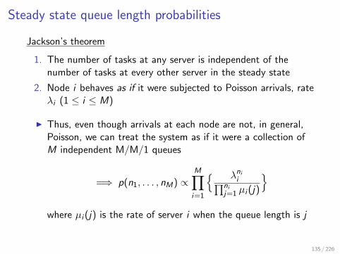
Jackson’s theorem
1. The number of tasks at any server is independent of thenumber of tasks at every other server in the steady state
2. Node i behaves as if it were subjected to Poisson arrivals, rateλi (1 ≤ i ≤ M)
I Thus, even though arrivals at each node are not, in general,Poisson, we can treat the system as if it were a collection ofM independent M/M/1 queues
=⇒ p(n1, . . . , nM) ∝M∏i=1
λnii∏ni
j=1 µi (j)
where µi (j) is the rate of server i when the queue length is j
135 / 226

I If service rates are constant, µi ,
p(n) ≈M∏i=1
ρnii =
M∏i=1
(1− ρi )ρnii
where ρi = λiµi
I p(n)→ usual performance measures such as mean queuelengths, utilisations, throughput by standard methods – meanwaiting times by Little’s result
NoteThe normalising constant for p(n)|n ∈ S is not shown for thegeneral case: it is the product of those for the M/M/1 queues.
136 / 226
Mean Value analysis
I Can exploit Jackson’s theorem directly, together with Little’sresult, if only average quantities are required
I values for mean queue lengths Li are those for isolated M/M/1queues with arrival rates λi (1 ≤ i ≤ M)
I assuming constant service rates µi
Li =ρi
1− ρifor 1 ≤ i ≤ M
(average number of tasks at node i)I total average number of tasks in network
L =M∑i=1
Li =M∑i=1
ρi
1− ρi
137 / 226

I Waiting timesI Average waiting time in the network, W = L/γ by Little’s
result where γ =∑M
i=1 γi is the total arrival rateI Average time spent at node i during each visit
Wi = Li/λi =1
µi (1− ρi )
I Average time spent queueing on a visit to node i
WQi = LQi/λi =ρi
µi (1− ρi )
138 / 226

An alternative formulation
I Let vi be the average number of visits made by a task toserver i
γvi = average number of arrivals to node i in unit time = λi
where γ is the average number of arrivals to the wholenetwork in unit time and vi the average number of visits agiven arrival makes to node i
vi =λi
γ(1 ≤ i ≤ M)
I Let Di be the total average service demand on node i fromone task
Di =vi
µi=ρi
γ
ρi = γDi = average work for node i arriving from outside thenetwork in unit time
139 / 226

I Often specify a queueing network directly in terms ofDi |1 ≤ i ≤ M and γ; then there is no need to solve thetraffic equations
I
Li =ρi
1− ρi=
γDi
1− γDi
L and W as before
I Let Bi = total average time a task spends at node i
Bi = viWi =vi
µi (1− ρi )=
Di
1− γDi
alternatively apply Little’s result to node i with the externalarrival process directly
Bi =Li
γ=
Di
1− γDi
140 / 226

I However, Di and γ cannot be used to determine µi and henceneither Wi nor Ri
I Specification for delay nodes (IS) iI Li = ρi = γDi
I Bi = Di (no queueing)I Wi = 1/µi
I Di = vi/µi (as for any work conserving discipline also)I service time distribution arbitrary
141 / 226

Distribution of time delays
I Even though arrivals at each node are not, in general, Poisson,the Random Observer Property still holds: waiting timedistribution at node i is exponential, parameter µi − λi againas expected from Jackson’s theorem.
I Networks with no overtaking (“tree-like” networks) are easyto solve for time delay distributions:
142 / 226
1
4
5
3
2
route r = (1,2,3)
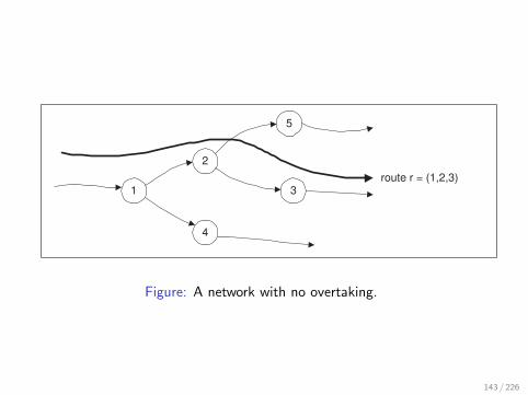
Figure: A network with no overtaking.
143 / 226
I sojourn time on any route is the sum of independent,exponential random variables
I this argument is independent of Jackson’s theorem and oneproof uses the idea of reversibility of the M/M/1 queue
I time delay distribution is a convolution of exponentials, e.g.f1 ? f2 ? f3 for route r where fi (t) = (µi − λi )e−(µi−λi )t fori = 1, 2, 3.
144 / 226

Time delays in general networks
I mean sojourn time for any route is always easy because themean of a sum of random variables is equal to the sum of themeans of those random variables, whether or not they areindependent
I in networks with overtaking, the distribution of route sojourntimes remains an open problem. For example, in the network
145 / 226

1 3
2
overtaking possible
no overtaking
Figure: A network with overtaking.
146 / 226
I I sojourn time distribution on route 1→ 3 is the convolution of2 exponentials
I sojourn time distribution on route 1→ 2→ 3 is not theconvolution of 3 exponentials because the queue length facedat node 3 upon arrival depends on the number of departuresfrom node 1 during the sojourn time at node 2.
I The Random Observer Property is not applicable since thearrival to node 3 is not random when conditioned on theprevious arrival at node 1.
I Jackson’s theorem does not apply because it is concerned onlywith steady state probabilities, i.e. the asymptotic behaviourof pt(n) at the single point in time t as t →∞.
I Subject of many research papers.
147 / 226

Closed Queueing Networks
I No external arrivals or departures (no γi terms).
I Routing probabilities satisfy
M∑j=1
qij = 1 for 1 ≤ i ≤ M
I State space S = (n1, . . . , nM)|ni ≥ 0,∑M
j=1 nj = K forpopulation K
I |S | = # of ways of putting K balls into M bags =(K+M−1
M−1
)I finiteness of S → steady state always exists
148 / 226

I Traffic equations are
λi =M∑
j=1
λjqji for 1 ≤ i ≤ M
I homogeneous linear equations with an infinity of solutionswhich differ by a multiplicative factor (because |I − Q| = 0since rows all sum to zero)
I let (e1, . . . , eM) be any non-zero solution (typically chosen byfixing one ei to a convenient value, like 1)
therefore ei ∝ arrival rate λi , i.e. ei = cλi
xi = eiµi∝ load = ρi , i.e. xi = cρi
149 / 226

Steady state probability distribution for S
I Jackson’s theorem extends to closed networks which have aproduct form solution
p(n1, . . . , nM) =1
G
M∏i=1
enii∏ni
j=1 µi (j)where
M∑i=1
ni = K . (1)
where µi (j) is the service rate of the exponential server i whenits queue length is j .
I G is the normalising constant of the network
G =∑nnn∈S
M∏i=1
enii∏ni
j=1 µi (j)(2)
not easy to compute (see later)
150 / 226

I Prove the result by using the network’s steady state balanceequations:
Total flux out of state nnn = p(nnn)M∑i=1
µi (ni )ε(ni )
= Total flux into state nnn :∑i ,j
nnnji → nnn
=M∑i=1
M∑j=1
p(nnnji )ε(ni )µj((nnnj
i )j)qji
where ε(n) =
0 if n = 0
1 if n > 0
nnnji =
(n1, . . . , ni − 1, . . . , nj + 1, . . . , nM) if i 6= j
nnnii = nnn otherwise
151 / 226

note that (nnnji )j =
nj + 1 if i 6= j
ni otherwise
I Try
p(n1, . . . , nM) =1
G
M∏i=1
enii
ni∏j=1
µi (j)
where∑i=1
ni = K .
152 / 226

Then require
1
G
M∏i=1
eni
ini∏
j=1
µi (j)
∑
i
µi (ni )ε(ni ) =1
G
M∏i=1
eni
ini∏
j=1
µi (j)
∑
i,j :i=j
µi (ni )ε(ni )qji
+1
G
M∏i=1
eni
ini∏
j=1
µi (j)
×
∑i,j :i 6=j
ej
ei
µi (ni )
µj(nj + 1)ε(ni )µj(nj + 1)qji
i.e. ∑i
µi (ni )ε(ni ) =∑
i
µi (ni )ε(ni )
∑j ejqji
ei
which is satisfied if eee satisfies the traffic equations.
153 / 226

I Note that if eee ′ = ceee is another solution to the trafficequations, the corresponding probabilities p′(nnn) and G ′ are
p′(nnn) =1
G ′Gc
Pni p(nnn) =
GcK
G ′p(nnn)
G ′ = cK G =∑nnn∈S
GcP
ni p(nnn)
and therefore p′(nnn) = p(nnn). This confirms the arbitrariness ofeee up to a multiplicative factor.
154 / 226

Computation of the normalising constant
I We consider only the case of servers with constant servicerates to get an efficient algorithm.
I There are also algorithms for networks with servers havingstate dependent service rates, e.g. the convolution algorithm.
I Less efficient but important since the alternative MVAalgorithm also requires constant rates.
155 / 226

I Define G = g(K ,M) where
g(n,m) =∑
n∈S(n,m)
m∏i=1
xnii
where S(n,m) = (n1, . . . , nm)|ni ≥ 0,∑m
i=1 ni = n andxi = ei
µi(1 ≤ i ≤ m).
I state space for subnetwork of nodes 1, 2, . . . ,m and populationn.
156 / 226

I For n,m > 0
g(n,m) =∑
n∈S(n,m),nm=0
m∏i=1
xnii +
∑n∈S(n,m),nm>0
m∏i=1
xnii
=∑
n∈S(n,m−1)
m−1∏i=1
xnii + xm
∑ki =ni (i 6=m)km=nm−1n∈S(n,m)
m∏i=1
xkii
= g(n,m − 1) + xmg(n − 1,m)
because k |ki ≥ 0;m∑
i=1
ki = n − 1 = S(n − 1,m).
157 / 226

I Boundary conditions:
g(0,m) = 1 for m > 0
g(n, 0) = 0 for n ≥ 0
I Note
g(0,m) =∑
n=(0,...,0)
m∏i=1
x0i = 1
andg(n, 1) = x1g(n − 1, 1) = xn
1
158 / 226

Marginal queue length probabilities and performancemeasures
I Although p(k) ∝∏
pi (ki ) it is not the case thatP(Ni = ki ) = pi (ki ), as in the open networks. The use ofM/M/1 factors is just a convenient mathematical device,there is no probabilistic interpretation.
I Probability that a server is idle (= 1− utilisation)
P(NM = 0) =1
g(K ,M)
∑n∈S(n,m),nm=0
M−1∏i=1
xnii =
g(K ,M − 1)
g(K ,M).
In general
P(Ni = 0) =Gi (K )
G (K )for 1 ≤ i ≤ M
159 / 226
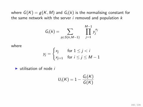
where G (K ) = g(K ,M) and Gi (k) is the normalising constant forthe same network with the server i removed and population k
Gi (k) =∑
n∈S(k,M−1)
M−1∏j=1
ynj
j
where
yj =
xj for 1 ≤ j < i
xj+1 for i ≤ j ≤ M − 1
I utilisation of node i
Ui (K ) = 1− Gi (K )
G (K )
160 / 226

Alternative Formulation: Cumulative Probabilities
I For 1 ≤ k ≤ K and 1 ≤ i ≤ M
P(Ni ≥ k) =∑
n∈S(K ,M),ni≥k
M∏j=1
xnj
j
G (K )
=xki
G (K )
∑mi =ni−k
ni≥k mj =nj (j 6=i)n∈S(K ,M)
M∏j=1
xmj
j
=xki
G (K )
∑m∈S(K−k,M)
M∏j=1
xmj
j
= xki
G (K − k)
G (K ).
161 / 226

Therefore the utilisation is given by
Ui = xiG (K − 1)
G (K )
I Equating two expressions for Ui yields the recurrence relationfor g(k ,m) previously
I Throughput of server i ,
Ti (k) = µiUi (k) = eiG (K − 1)
G (K )
proportional to visitation rate as expected.
162 / 226

I Queue length distribution at server i is P(Ni = k) = pi (k) for0 ≤ k ≤ K and 1 ≤ i ≤ M
pi (k) = P(Ni ≥ k)− P(Ni ≥ k + 1)
= xki
G (K − k)− xiG (K − k − 1)
G (K ).
where G (−1) = 0 by definition.
163 / 226

I Notice that the previous formulation gives a more conciseformulation for pi (k)
pi (k) =1
G (K )
∑n∈S(K ,M),ni =k
M∏j=1
xnj
j
=xki
G (K )
∑n∈S(K−k,M),ni =0
M∏j=1
xnj
j
= xki
Gi (K − k)
G (K )
for 0 ≤ k ≤ K and 1 ≤ i ≤ M. This is a generalisation of theresult obtained for Ui (k).
164 / 226

I Mean queue length at server i , 1 ≤ i ≤ M, Li (k)
Li (K ) =K∑
k=1
kP(Ni = k)
=K∑
k=1
P(Ni ≥ k)
=
∑Kk=1 xk
i G (K − k)
G (K ).
165 / 226

Equivalent open networks and the use of mean valueanalysis
I Consider an irreducible network – one in which every arc istraversed within finite time from any given time withprobability 1
Closed
Network
0
arc a2
arc a1
arc a
arrivals
departures
Figure: Equivalent open network.
166 / 226

I i.e. a network represented by an irreducible positive recurrentMarkov process (finite state space)
I we introduce a node, 0, in one of the arcs and replace arc a byarc a1, node 0 and arc a2
I Source of a1 is source of aI destination of a2 is destination of a
I Whenever a task arrives at node 0 (along arc a1), it departsfrom the network and is immediately replaced by astochastically identical task which leaves node 0 along arc a2
I Define the network’s throughput, T , to be the average rate atwhich tasks pass along arc a in the steady state.
I i.e. T is mean number of tasks traversing a in unit time.I One can choose any arc in an irreducible network.
167 / 226

Visitation rates and application of Little’s result
I Let the visitation rate be vi and the average arrival rate be λi
for node i , 1 ≤ i ≤ M, then λi = Tvi where T is the externalarrival rate.
I The set vi |1 ≤ i ≤ M satisfies the traffic equations, as wecould have derived directly by a similar argument.
I Suppose arc a connects node α to node β in the closednetwork 1 ≤ α, β ≤ M, then v0 = vαqαβ because all trafficfrom α to β goes through node 0 in the open network.
I But every task enters node 0 exactly once, hence vα = 1qαβ
since v0 = 1. This determines vi |1 ≤ i ≤ M uniquely.
168 / 226

I Little’s result now yields
Li = λiWi = TviWi
M∑i=1
Li = K = TM∑i=1
viWi
since the sum of all queue lengths is exactly K in the closednetwork
=⇒ T =K∑M
i=1 viWi
169 / 226

Mean waiting times
I
Wi =1
µi[1 + Yi ]
where the first term is the arriving task’s mean service timeand Yi is the mean number of tasks seen by new arrivals atserver i .
I For an IS (delay) server Wi = 1µi
, otherwise . . .
I Do not have the random observer propertyI number of tasks seen on arrival does not have the same steady
state distribution as the queue length since K tasks are seenwith probability 0. (arrival cannot “see itself”)
I do not have Yi = L− 1 as in open networks
170 / 226

I Do have the analogous Task (or Job) Observer Property:The state of a closed queueing network in equilibrium seen bya new arrival at any node has the same distribution as that ofthe state of the same network in equilibrium with the arrivingtask removed (i.e. with population K − 1)
I arriving task behaves as a random observer in a network withpopulation reduced by one
I intuitively appealing since the “one” is the task itselfI but requires a lengthy proof (omitted)
171 / 226
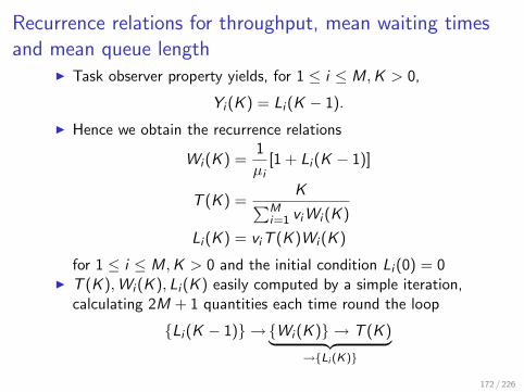
Recurrence relations for throughput, mean waiting timesand mean queue length
I Task observer property yields, for 1 ≤ i ≤ M,K > 0,
Yi (K ) = Li (K − 1).
I Hence we obtain the recurrence relations
Wi (K ) =1
µi[1 + Li (K − 1)]
T (K ) =K∑M
i=1 viWi (K )
Li (K ) = viT (K )Wi (K )
for 1 ≤ i ≤ M,K > 0 and the initial condition Li (0) = 0I T (K ),Wi (K ), Li (K ) easily computed by a simple iteration,
calculating 2M + 1 quantities each time round the loop
Li (K − 1) →Wi (K ) → T (K )︸ ︷︷ ︸→Li (K)
172 / 226

Alternative formulation
I Total average time spent at node i when population is K
Bi (K ) = viWi (K )
for 1 ≤ i ≤ M
I Total average service time (demand) a task requires fromnode i
Di =vi
µi
for 1 ≤ i ≤ M independent of population K .
173 / 226

I Therefore
Bi (K ) = Di [1 + Li (K − 1)]
T (K ) =K∑M
i=1 Bi (K )
Li (K ) = T (K )Bi (K )
for 1 ≤ i ≤ M
I Total average time in network spent by a task
W (K ) =M∑i=1
viWi (K ) =M∑i=1
Bi (K ) =K
T (K )
as expected by Little’s law
174 / 226
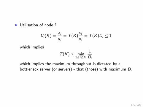
I Utilisation of node i
Ui (K ) =λi
µi= T (K )
vi
µi= T (K )Di ≤ 1
which implies
T (K ) ≤ min1≤i≤M
1
Di
which implies the maximum throughput is dictated by abottleneck server (or servers) - that (those) with maximum Di
175 / 226

A faster approximate algorithm
I Algorithms given above need to evaluate 2M + 1 quantitiesfor each population between 1 and K
I Would be faster if we could relate Yi (K ) to Li (K ) rather thanLi (K − 1), which implies that we do not need to worry aboutpopulations less than K
I
Yi (K ) =K − 1
KLi (K )
is a good approximation, exact for K = 1 and correctasymptotic behaviour as K →∞ (exercise)
176 / 226

I then
Bi (K ) = Di
[1 +
K − 1
KT (K )Bi (K )
]I
Bi (K ) =Di
1− K−1K DiT (K )
I Thus we obtain the fixed point equation
T (K ) = f (T (K ))
where
f (x) =K∑M
i=1Di
1−K−1K
Dix
there are many numerical methods to solve such equations
177 / 226
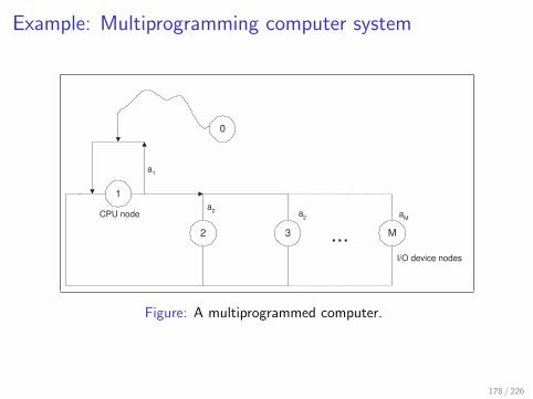
Example: Multiprogramming computer system
1
M 3 2
0
...
a 1
a 2
a 2
a M
I/O device nodes
CPU node
Figure: A multiprogrammed computer.
178 / 226
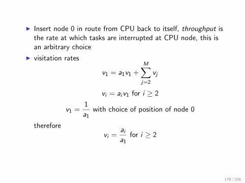
I Insert node 0 in route from CPU back to itself, throughput isthe rate at which tasks are interrupted at CPU node, this isan arbitrary choice
I visitation rates
v1 = a1v1 +M∑
j=2
vj
vi = aiv1 for i ≥ 2
v1 =1
a1with choice of position of node 0
thereforevi =
ai
a1for i ≥ 2
179 / 226

I Sanity check: is the first equation is satisfied?
Di =ai
a1µifor i ≥ 2
D1 =1
a1µ1
therefore T (K ) follows by solving recurrence relations
I total CPU throughput = T (K)a1
(fraction a1 recycles)
180 / 226

Application: A batch system with virtual memory
I Most medium-large computer systems use virtual memory
I It is well-known that above a certain degree ofmultiprogramming performance deteriorates rapidly
I Important questions areI How does the throughput and turnaround time vary with the
degree of multiprogrammingI What is the threshold below which to keep the degree of
multiprogramming?
181 / 226

Representation of paging
I Suppose node 2 is the paging device (e.g. fast disk)I assume dedicated to pagingI easy to include non-paging I/O also
I We aim to determine the service demand of a task at node 2,D2, from tasks’ average paging behaviour
I use results from ’70s working set theoryI consider the page fault rate for varying amounts of main store
allocated to a task
I Let the population be K
182 / 226

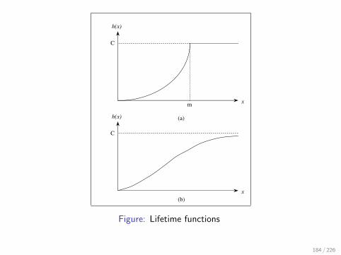
I paging behaviour will be represented by a lifetime function:I h(x) = average CPU time between consecutive page faults
when a task has x pages of memoryI h(0) ≈ 0 (the first instruction causes a fault)I h(x) = C , the total CPU time of a task for x ≥ some constant
value m, where m is the “size” of the taskI h is an increasing function: the more memory a task has the
less frequent will be its page faults on average.I Two possible types of lifetime functions:
183 / 226
C
m
h(x)
x
(a)
C
h(x)
x
(b)
Figure: Lifetime functions
184 / 226
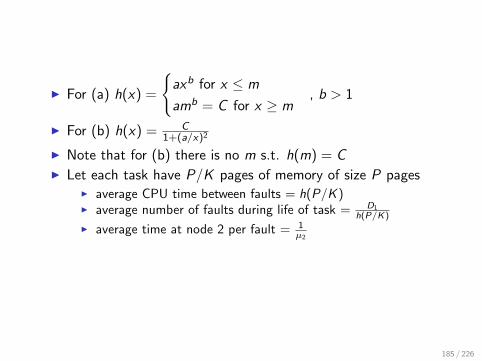
I For (a) h(x) =
axb for x ≤ m
amb = C for x ≥ m, b > 1
I For (b) h(x) = C1+(a/x)2
I Note that for (b) there is no m s.t. h(m) = CI Let each task have P/K pages of memory of size P pages
I average CPU time between faults = h(P/K )I average number of faults during life of task = D1
h(P/K)
I average time at node 2 per fault = 1µ2
185 / 226
I Therefore average paging time of a task (from node 2)I D2 = H(K ) = D1
µ2h(P/K)I D2 = d2 + H(K ) if average non-paging requirement of a task
from node 2 is d2
I As K →∞, T (K )→ 0 since T (K ) ≤ min 1Di
and D2 →∞
186 / 226

Solution
I We again use the alternative form of the MVA algorithm
I For population K and 1 ≤ k ≤ K
Bi (k) = Di (K )[1 + Li (k − 1)] (1 ≤ i ≤ M)
T (k) =k∑M
i=1 Bi (k)
Li (k) = T (k)Bi (k) (1 ≤ i ≤ M)
I Notice that only D2 is a function of K − D1 and D3 areconstant
187 / 226

I Computation for a range of populations requires 2 nestedloops:
I outer loop for K = 1, 2, . . . ,Kmax
I inner loop for k = 1, 2, . . . ,KI need new value for H(K ) each time round the outer loop
188 / 226

Choice of lifetime function
We assume (arbitrarily) the lifetime function
h(x) =
D1( x
10000 )3.5, x ≤ 10000
D1 otherwise
for all tasks, i.e.
Life-time function example
0
0.1
0.2
0.3
0.4
0.5
0.6
0.7
0.0 3.0 6.0 9.0 12.0 15.0 18.0
Available memory (Kpages)
Mea
n t
ime
bet
wee
n f
au
lts
Figure: Lifetime function example.
189 / 226

Thrashing curves
Mean job processing time vs. number of jobs
0
100
200
300
400
500
600
700
0 2 4 6 8
10
12
14
16
18
20
22
24
26
28
30
32
34
36
38
40
Number of jobs
W
Figure: Mean job processing time vs. number of jobs.
190 / 226

Throughput vs. number of jobs
0
0.1
0.2
0.3
0.4
0.5
0.6
0.7
0.8
0 2 4 6 8
10
12
14
16
18
20
22
24
26
28
30
32
34
36
38
40
Number of jobs
Th
rou
gh
pu
t
Figure: Throughput vs. number of Jobs.
191 / 226
Decomposition
I Separable queueing models are prone to break down in somesituations:
I There is usually a good model for small parts of any networkI Composing the bits can be hard unless the criteria for
separability are (reasonably) met
I Ideally, we need a method to:I Reduce complexity (breaking a large problem into smaller
manageable ones)I Provide approximate solutions where the necessary
assumptions do not hold
192 / 226

I The most powerful general method is decomposition(sometimes called aggregation)
I The idea is to replace a subnetwork of a (complex) systemwith a single flow-equivalent server (FES)
F.E.S.
Subnetwork
Figure: Flow equivalent server.
193 / 226
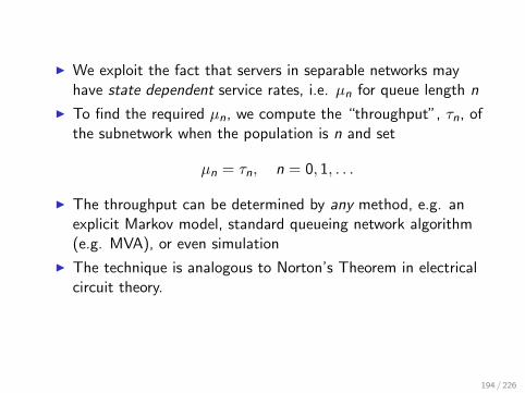
I We exploit the fact that servers in separable networks mayhave state dependent service rates, i.e. µn for queue length n
I To find the required µn, we compute the “throughput”, τn, ofthe subnetwork when the population is n and set
µn = τn, n = 0, 1, . . .
I The throughput can be determined by any method, e.g. anexplicit Markov model, standard queueing network algorithm(e.g. MVA), or even simulation
I The technique is analogous to Norton’s Theorem in electricalcircuit theory.
194 / 226
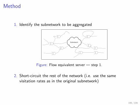
Method
1. Identify the subnetwork to be aggregated
Subnetwork
Figure: Flow equivalent server — step 1.
2. Short-circuit the rest of the network (i.e. use the samevisitation rates as in the original subnetwork)
195 / 226

Subnetwork
Figure: Flow equivalent server — step 2.
I Compute the throughput τn, on the short-circuit arc for allpopulations 0, 1, . . .
Population n
Throughput = n
Figure: Flow equivalent server — step 3.
196 / 226

I Define a single FES with service rate µn = τn, n = 0, 1, . . .
I Replace the subnetwork with the FES and re-solve
FES
Figure: Flow equivalent server — step 5.
197 / 226
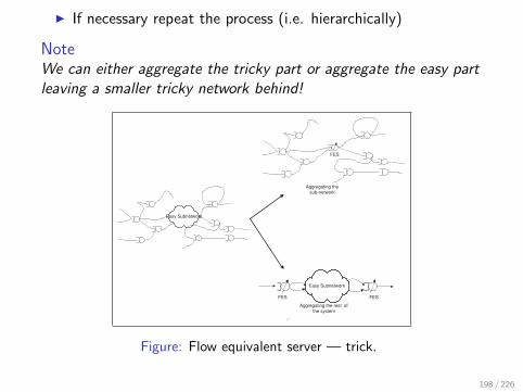
I If necessary repeat the process (i.e. hierarchically)
NoteWe can either aggregate the tricky part or aggregate the easy partleaving a smaller tricky network behind!
FES
Aggregating the
sub-network
Easy Subnetwork
FES FES
Aggregating the rest of
the system
Easy Subnetwork
Figure: Flow equivalent server — trick.
198 / 226
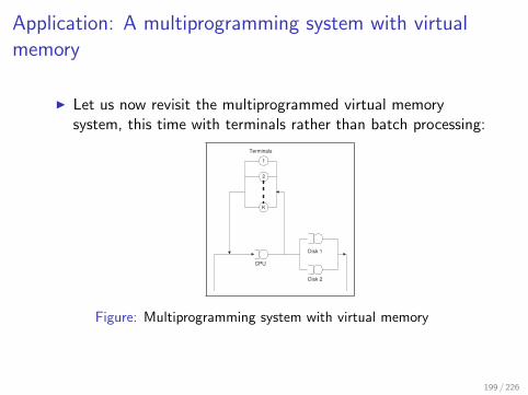
Application: A multiprogramming system with virtualmemory
I Let us now revisit the multiprogrammed virtual memorysystem, this time with terminals rather than batch processing:
2
Terminals
Disk 2
CPU
1
K
Disk 1
Figure: Multiprogramming system with virtual memory
199 / 226

I The average think time of each user is 30 seconds
I Q: How does the system throughput and response time varywith the number of terminals, K , and at what point does thesystem start to thrash?
I As users submit jobs, they increase the population at thecomputer system and consume memory
I The problem is that the performance of the computersubsystem depends on the number of jobs there
I But the number of jobs at the subsystem is governed by thenumber of terminals
I Specifically, the Disk 1 service rate depends on the populationof the entire subnetwork: no simple (product-form) solution
200 / 226

2
Terminals
Disk 2
CPU
1
K
Disk 1
Figure: Multiprogramming system with virtual memory — step 1
201 / 226

I In the batch model we computed previously thethroughput,τn, when there were n batch jobs being processed
I We can thus aggregate the server subsystem into aflow-equivalent server whose service rate at population n is
µn = τn
I That is
2
Terminals
1
K
FES
Figure: Multiprogramming system with virtual memory - FES
202 / 226
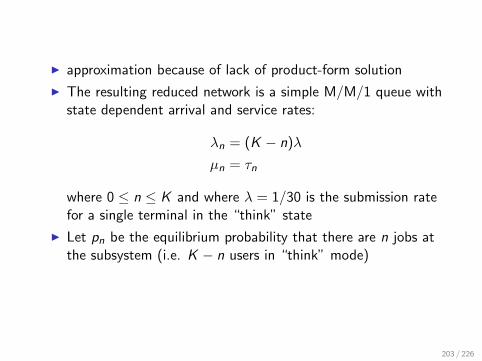
I approximation because of lack of product-form solution
I The resulting reduced network is a simple M/M/1 queue withstate dependent arrival and service rates:
λn = (K − n)λ
µn = τn
where 0 ≤ n ≤ K and where λ = 1/30 is the submission ratefor a single terminal in the “think” state
I Let pn be the equilibrium probability that there are n jobs atthe subsystem (i.e. K − n users in “think” mode)
203 / 226
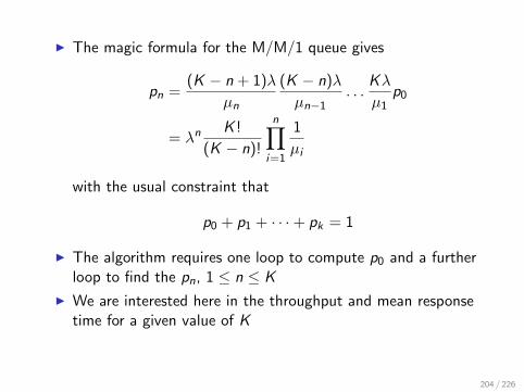
I The magic formula for the M/M/1 queue gives
pn =(K − n + 1)λ
µn
(K − n)λ
µn−1. . .
Kλ
µ1p0
= λn K !
(K − n)!
n∏i=1
1
µi
with the usual constraint that
p0 + p1 + · · ·+ pk = 1
I The algorithm requires one loop to compute p0 and a furtherloop to find the pn, 1 ≤ n ≤ K
I We are interested here in the throughput and mean responsetime for a given value of K
204 / 226

I The throughput is:
τ = p0µ0 + p1µ1 + · · ·+ pKµK
I We next need to find the mean population of the subsystem:
L = 0× p0 + 1× p1 + · · ·+ K × pK
I The mean waiting time then follows from Little’s law
W = L/τ
I With the same paging model as the batch system earlier, thisis what happens to τ as we increase K
205 / 226
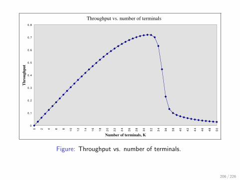
Throughput vs. number of terminals
0
0.1
0.2
0.3
0.4
0.5
0.6
0.7
0.8
0 2 4 6 8
10
12
14
16
18
20
22
24
26
28
30
32
34
36
38
40
42
44
46
48
50
Number of terminals, K
Th
rou
gh
pu
t
Figure: Throughput vs. number of terminals.
206 / 226

I The saturation point is clear! Beyond this the meanpopulation of the computer subsystem is such that thrashingoccurs
I Here is the behaviour of the mean waiting time as we increaseW
Mean response time vs. number of terminals
0
200
400
600
800
1000
1200
1400
1600
1800
0 2 4 6 8
10
12
14
16
18
20
22
24
26
28
30
32
34
36
38
40
42
44
46
48
50
Number of terminals, K
W
Figure: Mean response time vs. number of terminals.
207 / 226

I And finally (for the record), here is L:
Central server population vs. number of terminals
0
5
1 0
1 5
2 0
2 5
3 0
3 5
4 0
4 5
5 0
0 2 4 6 8
10
12
14
16
18
20
22
24
26
28
30
32
34
36
38
40
42
44
46
48
50
Number of terminals, K
Mea
n n
um
ber
of
use
rs w
ait
ing, L
Figure: Central server population vs. number of terminals.
208 / 226

The Markov Modulated Poisson Process (MMPP)
I Poisson process is a good model for many arrival streamsI more short interarrival times than longI superposition of many sparse independent renewal processes is
asymptotically PoissonI right intuitive properties given minimal information (i.e. arrival
rate)
I But cannot model many characteristics seen in modernnetworks
I multiple traffic types with known switching pattern betweentypes
I correlated traffic, i.e. non-zero correlation between interarrivaltimes
I self-similarity
209 / 226
I MMPP accounts for some of these limitationsI models stochastically changing modes with different ratesI has non-zero autocorrelation which can be calculatedI integrates well into queueing models – the MMPP/M/1 queue
210 / 226
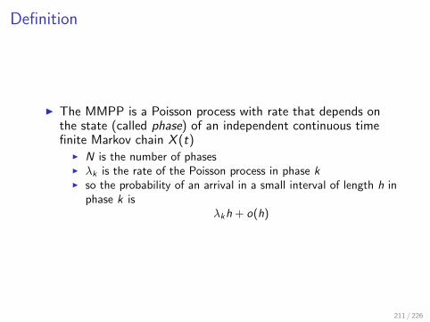
Definition
I The MMPP is a Poisson process with rate that depends onthe state (called phase) of an independent continuous timefinite Markov chain X (t)
I N is the number of phasesI λk is the rate of the Poisson process in phase kI so the probability of an arrival in a small interval of length h in
phase k isλkh + o(h)
211 / 226
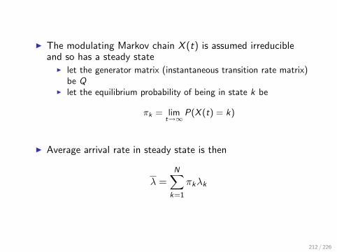
I The modulating Markov chain X (t) is assumed irreducibleand so has a steady state
I let the generator matrix (instantaneous transition rate matrix)be Q
I let the equilibrium probability of being in state k be
πk = limt→∞
P(X (t) = k)
I Average arrival rate in steady state is then
λ =N∑
k=1
πkλk
212 / 226

State at Arrival Instants
I Important for response time distributions
I Do not have the Random Observer Property
I In a long period of time T at equilibriumI expected time spent in state k is πkTI expected number of arrivals that see state k = λkπkTI total number of arrivals has mean λT
I So probability that an arrival sees state k in steady state is
π′k =λkπk
λ
213 / 226
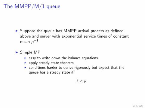
The MMPP/M/1 queue
I Suppose the queue has MMPP arrival process as definedabove and server with exponential service times of constantmean µ−1
I Simple MPI easy to write down the balance equationsI apply steady state theoremI conditions harder to derive rigorously but expect that the
queue has a steady state iff
λ < µ
214 / 226

I The MP has a 2-dimensional state spaceI phase of the MMPP horizontally (say)I queue length verticallyI infinite lattice strip for unbounded queue
I Let the steady state probability for phase k and queue lengthj be denoted by πjk and let the vector vj = (πj1, πj2, . . . , πjN)
I Balance equations are, for state (i , j + 1)
πj+1,i
λi + µ+∑k 6=i
qik
=∑k 6=i
πj+1,kqki + λiπj ,i + µπj+2,i
215 / 226

The MMPP/M/1 queue (continued)
I This may be written in matrix form as
vjΛ + vj+1(Q − Λ− µI ) + µvj+2I = 0
where I is the unit N × N matrix and Λ is the diagonal matrixwith the arrival rates λk down the diagonal, i.e.Λ = diag(λ1, . . . , λN)
I For states (i , 0) we get
v0(Q − Λ) + µv1I = 0
216 / 226

I The normalising equation is
∞∑j=0
vj · (1, 1, . . . , 1) = 1
I These equations give the unique equilibrium probabilities ifλ < µ
217 / 226

Exact solution methods
I We have a matrix recurrence relation of the form
vjQ0 + vj+1Q1 + vj+2Q2 = 0
for j ≥ 0 and constant matrices Q0,Q1,Q2
I Spectral Analysis (Chakka and Mitrani; see Mitrani’s book,last chapter)
218 / 226
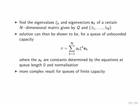
I find the eigenvalues ξk and eigenvectors ek of a certainN−dimensional matrix given by Q and (λ1, . . . , λN)
I solution can then be shown to be, for a queue of unboundedcapacity
π =N∑
k=1
akξkek
where the ak are constants determined by the equations atqueue length 0 and normalisation
I more complex result for queues of finite capacity
219 / 226

I Matrix Geometric MethodI Closely related to Spectral Analysis but a completely different
approachI Try a solution of the form vj = M ju for some matrix M and
vector uI Then solve
Q0 + MQ1 + M2Q2 = 0
for MI u from the other equations
220 / 226

Approximate solution methods
I It often happens that phase changes are rare in comparison toarrivals and departures
I rates in Q-matrix << λ1, . . . , λN , µI e.g. phase changes represent change of traffic type, such as
data, video, voice
I Often then a good approximation to use (an approximate)decomposition, cf. queueing networks
221 / 226

I For each phase k , solve the M/M/1 queue assuming the
arrival rate is constant, λk , giving equilibrium probability p(k)j
for queue length j , 1 ≤ k ≤ NI i.e. solve all the ‘columns’ in the 2-D state spaceI can only work if every λk < µ
I Then solve the phase process for the equilibrium probability rkof being in phase k , i.e. solve
r · Q = 0
I Approximate the solution by
πjk = p(k)j rk
222 / 226

Fitting MMPPs
I MMPP can be fitted to observed data by matching:I average arrival rate λ (or mean interarrival time)I higher moments of interarrival time (variance etc.)I autocorrelation function (ACF)I Hurst parameter, a measure of self-similarity
I Matching moments is easy but often gives a poor match oncorrelation, the main reason for using the MMPP in the firstplace!
223 / 226

I Can use ACF to model correlated traffic directlyI next slideI computationally difficult and expensiveI possibly use spectral methods, cf. Fourier transforms
I Hurst parameter gives a good representation of ‘howcorrelated’ traffic is, but only contributes one parameter in thematching process
I Better used to validate another matching process
224 / 226

Autocorrelation function of the MMPP
I The autocorrelation function at lag k ≥ 1 for the aboveMMPP is
ρk =π∗R−2Λ[I − eπ∗R−1ΛR−1Λk−1]R−2Λe
2π∗R−3Λe− (π∗R−2Λe)2
where the matrix R = Λ−Q, e = (1, 1, . . . , 1) and π∗ = πΛπ.λ .
I Autocorrelation function is easily calculated by the aboveformula, given the parameters of the MMPP
225 / 226

I But the converse, to determine the parameters from the ACF,is hard!
I gives non-linear equations in several variables (the sought-afterparameters)
I fixed point methods of solution tend to be unstableI research area
226 / 226
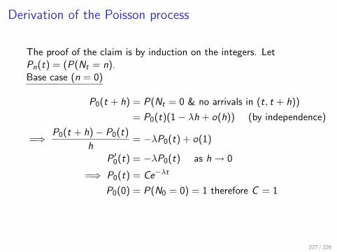
Derivation of the Poisson process
The proof of the claim is by induction on the integers. LetPn(t) = (P(Nt = n).Base case (n = 0)
P0(t + h) = P(Nt = 0 & no arrivals in (t, t + h))
= P0(t)(1− λh + o(h)) (by independence)
=⇒ P0(t + h)− P0(t)
h= −λP0(t) + o(1)
P ′0(t) = −λP0(t) as h→ 0
=⇒ P0(t) = Ce−λt
P0(0) = P(N0 = 0) = 1 therefore C = 1
227 / 226

Inductive Step (n > 0)
Pn(t + h) = Pn(t)P0(h) + Pn−1(h)P1(h) + o(h)
= (1− λh)Pn(t) + λhPn−1(t) + o(h)
=⇒ P ′n(t) = −λPn(t) + λPn−1(t)
=⇒ d
dt(eλtPn(t)) = λeλtPn−1(t)
228 / 226

Inductive hypothesis:
Pn−1(t) = e−λt (λt)n−1
(n − 1)!
This is OK for n = 1. Then
d
dt(eλtPn(t)) =
(λ)n
(n − 1)!tn−1
=⇒ eλtPn(t) =(λt)n
(n)!+ D
For t = 0, Pn(t) = 0 for n ≥ 2 and so D = 0. Thus
Pn(t) = e−λt λt
n!
229 / 226

I Associated with each arc in a state transition diagram is arate, e.g.:
j
i
k
r j,i
r i,a
r i,b
r i,c
r k,i
Figure: Transition rates in Markov chains
230 / 226

I The state holding time depends on the departure rates(1/(ri ,a + ri ,b + ri ,c) is the mean holding time for state i in theexample).
I The probability flux from a state i to a state j is the averagenumber of transitions from i → j per unit time at equilibrium:
Probability flux(i → j) = ri ,jpi
I At equilibrium (if it exists) the total flux into each state mustbalance the total flux out of it
I For example, in the example, for state i alone:
(ri ,a + ri ,b + ri ,c)pi = rj ,ipj + rk,ipk
231 / 226
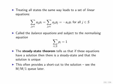
I Treating all states the same way leads to a set of linearequations:∑
j 6=i
aijpi =∑j 6=i
ajipj = −aiipi for all j ∈ S
I Called the balance equations and subject to the normalisingequation ∑
i∈S
pi = 1
I The steady-state theorem tells us that if these equationshave a solution then there is a steady-state and that thesolution is unique
I This often provides a short-cut to the solution – see theM/M/1 queue later.
232 / 226